130

AMSE JOURNALS-2016-Series: Modelling A; Vol. 89; N°1; pp 130-142

Submitted July 2016; Revised Oct. 15, 2016, Accepted Dec. 10, 2016

The Calculation for the Induced Magnetic Field of Ferromagnetic

Objects Based on Scalar Potential Integral equation

Qiang Bian, Xiang-jun Wang, Yu-de Tong, Guo-hua Zhou

College of Electrical and Information Engineering, Naval University of Engineering,

China, Wuhan, (tongyude@126.com)

Abstract

How to calculate induced magnetic field of ferromagnetic objects is one of the most

important question in ship degaussing. Based on the surface integral equation of ferromagnetic

objects’ induced magnetic field, the scalar potential numeric calculation model is established and

the desingularized analysis solution is deduced out to solve the singularity problem in this model.

Then, the calculation process to fix the induced magnetic field of ferromagnetic object with this

model is elaborated. Finally, a magnetic-field measurement experiment for a hollow cylinder is

designed and the result shows that the method is highly efficient.

Keywords

Element surface integral, scalar potential, induced magnetic field calculation, singularity.

1. Introduction

As the ferromagnetic hull object placed in the earth’s magnetic field, the ship may get a

magnetization which creates a local anomaly of the field and makes the ship vulnerable to

detection and mines. To protect naval vessels from the magnetically actuated mines and

surveillance systems, marines worldwide are looking for the methods to reduce magnetic

anomaly for decades. Obviously, an important precondition for the implementation of the above

magnetic protection technique is to evaluate the magnetic field of the naval vessels. Therefore, as

a basic task in magnetic protection technique, the numeric calculation modeling technique for

ship magnetic field directly decides the level of the ship magnetic protection technique to some

extent.

131

The magnetization of ferromagnetic objects can be divided in two parts: the induced

magnetization and the remnant magnetization. Currently, the finite-element method (FEM) and

the integral equation method are the most conventional methods to forecast the vessels’ induced

magnetic field. FEM could be used to solve the Laplacian equation with the induced magnetic

field’s scalar potential. However, the major drawback of FEM is to set boundary condition and

divide a lager region to the discrete elements of huge quantity that makes the calculation very

large [1, 2]. On the other hand, with the integral equation method, only the region of vessel

should be divided that makes the elements number and the calculation decrease greatly [3-8].

Meanwhile, to accelerate the solving algorithm, several approaches have been developed to solve

the volume integral equation, for example, the conjugate-gradient fast Fourier transform (CG-

FFT) algorithms and the Fast Multi-pole Method (FMM) [9-13].

According to the surface integral equation of ferromagnetic objects’ induced magnetic field,

the scalar potential numeric calculation model is established and the de-singularized analysis

solution is deduced out to solve the singularity problem in this model. Then, the calculation

process to fix the induced magnetic field of ferromagnetic object with this model is elaborated.

Finally, a magnetic-field measurement experiment for a hollow cylinder is designed and the result

shows that the induced magnetic field of ferromagnetic objects can be calculated efficiently and

accurately with the method proposed in this paper.

2. The scalar magnetic potential model with element surface integral equation

As is showed in Fig. 1, V is the volume of ferromagnetic object, S is the surface, r is

the field point radius vector, r is the source radius point vector and M is the intensity of

magnetization.

Fig.1. The magnetization model for ferromagnetic objects

132

When there is no free current in this region, the scalar magnetic potential of the magnetized

ferromagnetic object is as follow [4-8].

1 1( ) ( ') '( )

4 | ' |Vdv

mφ r M rr r

(1)

Naturally, as a uniform magnetized object,

' 0 M (2)

Thanks to

( ) A A A (3)

And

V Sdv ds A A n (4)

Equation (1) can be simplified to

1 ( ')( )

4 | ' |m

Sds

M r n

rr r

(5)

Generally， it is impossible for the irregular ferromagnetic object to be magnetized

uniformly in external magnetic field. If the ferromagnetic object is divided to n little elements,

the every single dissection element can be taken as a uniform magnetized object when the volume

of the discrete dissection element is small enough and the induced potential can be given by

m

1

1 ( ')( ) ( ')

4 | ' |i

n

i s

ds

M r nr r r

r r (6)

133

3. The numerical calculation method of coupling factor based on irregular

hexahedron element

On behalf of the easy to calculate the coupling factor based on regular element, and also, the

commonality to dissect the complex objects with the irregular hexahedron element, we will

research the numerical calculation method of coupling factor based on irregular hexahedral

element.

Fig.2. The irregular hexahedral element

We can get nodes’ data of every irregular hexahedral element after the dissection of

ferromagnetic region. As usual, take the irregular hexahedral element as the research object

showed in Fig.2.

Thanks to (6), the scalar magnetic potential on P produced by the j-th irregular hexahedral

element can be given by

6

1

1 1( )

4 | ' |i

j j ij

i is

ds

r M nr r

(7)

Then, the scalar magnetic potential on P produced by the ferromagnetic region can be

calculated by

6

1 1

1 1( )

4 | ' |i

n

P j ij

j i is

ds

r M nr r

(8)

134

Inside each element, the scalar potential is approximated by linear function

1 2 3 4( , , ) (1, , , ) ( , , , )Tx y z x y z k k k k (9)

Substitute the scalar magnetic potentials and coordinate values of the irregular hexahedral

element’s eight nodes to (9), we can get a linear system of equations as follows

C K (10)

Where 1 2 3 4( , , , )TK k k k k , 1 2 3 4 5 6 7 8( , , , , , , , )T ,1 2 3 4 5 6 7 8

1 2 3 4 5 6 7 8

1 2 3 4 5 6 7 8

1 1 1 1 1 1 1 1T

x x x x x x x xC

y y y y y y y y

z z z z z z z z

Solve the equations, we can get

1K C (11)

Thanks to the uniform magnetization in the irregular hexahedral element,

1

2 3 4( , , )T

jM k k k I K I C (12)

Where

0 1 0 0

0 0 1 0

0 0 0 1

I

.

As a consequence, the scalar magnetic potential at node j is

6

1

61

1

1 1( )

4 | ' |

1 1

4 | ' |

i

i

j ij j

i is

ij

i is

ds

ds I C

r n Mr r

nr r

(13)

135

Thanks to (13), the key to calculate the coupling factor matrix based on the data of irregular

hexahedral element’s nodes is to solve this surface integral as follows

1( )

| ' |i is

f dsP

r r (14)

Where is (i=1, 2, …, 6) is the i-th surface of the element. Given the difficulty to get the

original function in the form expressed by primary functions, the numerical method is applied to

calculated (14). Because of the variable of shapes and coordinates in different dissection schemes,

it is difficult to calculate the surface integral in the global coordinate system. Then, we create a

local coordinate system A-XYZ as is showed in Fig. 3, (14) can be turned to

( ) ( , )

ABCDS

f F x y ds P (15)

Where 2 2 2

0 0 0( , ) 1/ ( ) ( )F x y x x y y z . ( , )x y and 0 0 0( , , )x y z are the coordinates

of the source point Q and the field point P.

Fig.3. The local coordinate system of the i-th surface in the irregular hexahedral element

As is showed in Fig.4, A-XYZ is the local coordinate system of the i-th surface in the

element and o-xyz is the global coordinate system.

136

Fig.4. The relation between the local and global coordinate systems of the i-th surface

The rotation matrix R from the global coordinate system to the local coordinate system is

given by

cos cos cos

cos cos cos

cos cos cos

Xx Yx Zx

Xy Yy Zy

Xz Yz Zz

R (16)

Where, UV is the included angle between the axis U of local coordinate system and the

axis V of global coordinate system and they can be set to x, y or z. Then, the field point

coordinate in the local coordinate system can be calculated by

0( )P P P R (17)

Where 0P is the coordinate of A.

In the local coordinate system, (15) can be calculated in four regions as is showed in Fig.5.

137

Fig.5. The integral region in the local coordinate system

Obviously, there will be a singularity of r in the integral when P and A is coincided. We can

eliminate the singularity by adopting the polar integral. Thanks to the polar integral, (15) can be

turned to

B

1( ) ( , ) .

+

ABCD ABCD

ABCD ADC A C

S S

S S S

f F x y ds rdrdr

drd drd drd

P

(18)

With Mathematical, its analytic expression could be deduced as follows

2 2Ln= ( )

( )ADC

c da

c d dS

x yX

x xdr

yd

(19)

where，

2 2 2

2 2 2 2 2

- ( )=

( ) ( )

c c d c c d d

a

c d d d c d d d d

x x x x x x yX

x x x y x x y x y

We can get the analytic expression of ABCS

drd by substituting ,( )d dx y with ( )b bx y in

(19)

Equation (13) is written at each node of the dissection to obtain a linear system as follows

138

0-S (20)

Where 0 is the vector which is composed with the scalar magnetic potential on each node

produced by the external magnetic field and is the total potential vector and S is the coupling

factor matrix. The total potential at each node is obtained by solving the linear system (20).

The total field at any point r0 is calculated thanks to

00 0 03

0

( ) ( )4

r

V

r rH r dv H r

r r

(21)

4. Calculation Example Based on Experimental Near Field

4.1 Experiment planning

A magnetic measurement experiment for a hollow cylinder with two capped terminals is

designed to prove the effectiveness of the numerical calculation method. The cylinder’s detailed

size and the planning of the experiment are shown in Fig.6. The geomagnetic field B0 in

experiment region is 34500nT.

Fig.6. The cylinder’s detailed size and the planning of the experiment

The accuracy of the magnetic-field measurement system is 1nT. The cylinder is fixed on the

non-magnetic trolley and the trolley’s moving is constrained along the north and south direction

139

on the non-magnetic rail while the sensors array is fixed on the rail. The measurement field point

is below the center keel of the cylinder. The longitudinal distance between two field points is

100mm and the total measured distance is 4400mm. The horizontal distance between two

magnetic sensors is 250mm. The vertical component of the cylinder’s magnetic field intensity on

the magnetic north and south is measured and their half of difference is the vertical component of

the cylinder’s induced magnetic field intensity.

4.2 The experiment’s calculation process and the analysis of the results

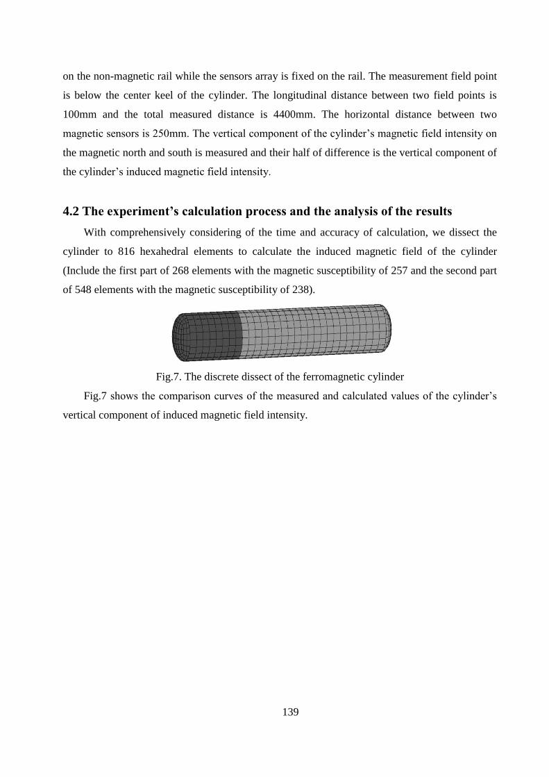
With comprehensively considering of the time and accuracy of calculation, we dissect the

cylinder to 816 hexahedral elements to calculate the induced magnetic field of the cylinder

(Include the first part of 268 elements with the magnetic susceptibility of 257 and the second part

of 548 elements with the magnetic susceptibility of 238).

Fig.7. The discrete dissect of the ferromagnetic cylinder

Fig.7 shows the comparison curves of the measured and calculated values of the cylinder’s

vertical component of induced magnetic field intensity.

140

Fig.8. The comparison between the calculated and the measured values of the induced

magnetic field on the measured points

As is shown in Fig.8, the measured and calculated values are corresponded perfectly and the

MSE between them is only 216.3 and the biggest relative error is 4.92％. The experiment results

show that the numerical calculation method based on the scar potential integral equation is of

high accuracy.

The model errors are produced by three parts as follows.

The error caused by the dissection error. Theoretically, the every single dissection element

can be taken as a uniform magnetized object only when the volume of the discrete dissection

element is infinitely small. However, the calculation will be impossible to be carried out by the

infinite number of elements. Therefore, the elements’ number should be reduced under the

premise of the calculation accuracy.

The measured error contains the inherent magnetic probe error, the manual operation error

and the measured errors caused by the environment.

The error caused by the linear approximation of scalar potential in the irregular hexahedral

element.

141

Discussion

The proposed model is established based on the scalar potential integral equation, which has

the advantages of a small amount of computation, low complexity and low memory occupation.

What's more, the singularity problem in the model can be solved perfectly by the de- singularized

analysis solution proposed in this paper. The proposed method will have an significant value in

induced magnetic field calculation.

Conclusion

A method to calculate the scalar magnetic potential of ferromagnetic objects based on the

surface integral equation is proposed in this paper. Firstly, the scalar potential numeric

calculation model is established based on the element surface integral method. Secondly, With

respect to the singularity problem in this model, the de-singularized analysis solution is deduced

out. Finally, a magnetic-field measurement experiment of a hollow cylinder with two capped

terminals is done, and the measured and calculation values are in good coincidence that proves

the effectiveness of the method proposed in this paper.

Acknowledgment

This work was supported by National Natural Science Foundation of China (Grant Nos.

51107145，61203193).

References

1. X. Brunotte, G. Meunier, J. Bongiraud, Ship magnetization modeling by the finite element

method, 1993, IEEE Transactions on Magnetics, vol. 29, no. 2, pp.1970-1976.

2. M.W. Fan, W.L. Yan, Integral equation method of the electromagnetic field, 1988, China

Machine Press, Beijing, pp.89-90.

3. C.B. Guo, D.M. Liu, B.C. Zhu, Calculation of induced magnetic fields of ships by integral

equation method, 2002, Journal of Naval University of Engineering, vol. 14, no. 3, pp.41-44.

4. G.H. Zhou, C.H. Xiao, H. Yan, A Method to Calculate Induced Magnetic Field of

Ferromagnetic Objects in Micro Magnetic Field, 2009, Journal of Harbin Engineering

University, vol. 30, no. 1, pp. 91-95.

142

5. G.H. Zhou, C.H. Xiao, S.D. Liu, Inversion Approach to Predicting the Magnetic Field

Distribution Based on Planar Field Measurements, 2010, International Journal of Applied

Electromagnetics and Mechanics, vol. 33, no. 3-4, pp.1033-1040.

6. O. Chadebec, J.L. Coulomb, J.P. Bongiraud, Recent Improvements for Solving Inverse

Magnetostatic Problem Applied to Thin Shells, 2002, IEEE Transactions on Magnetics, vol.

38, no. 2, pp.1005-1008.

7. Y. Vuillermet, O. Chadebec, J.L. Coulomb, Scalar Potential Formulation and Inverse Problem

Applied to Thin Magnetic Sheets, 2008, IEEE Transactions on Magnetics, vol. 44, no.6, pp.

1054-1057.

8. G.H. Zhou, C.H. Xiao, S.D. Liu, 3D magnetostatic field computation with hexahedral surface

integral equation method, 2009, Tansactions of China Electrotechnical Society, vol. 24, no.3,

pp. 1-7.

9. Q.H. Liu, W.C. Chew, Applications of the CG-FFHT method with an improved FHT

algorithm, 1994, Radio Sci., vol. 29, no. 4, pp. 1009-1022.

10. T.S. Nguyen, J.M. Guichon, O. Chadebec, Ships Magnetic Anomaly Computation With

Integral Equation and Fast Multipole Method, 2011, IEEE Trans. Magn, vol. 47, no. 5, pp.

1414-1417.

11. C. Jie, L. Xiwen, A new method for predicting the induced magnetic field of naval vessels,

2010, Acta Physica Sinica, vol. 59, no. 1, pp. 239-245.

12. Y.J. Liu, Fast multipole boundary element method theory and applications in engineering,

2009, Cambridge University Press, New York, pp.2-9.

13. T.J. Cui, W.C. Chew, Fast algorithm for electromagnetic scattering by buried 3D dielectric

objects of large size, 1999, IEEE Trans. Geosci. Remote Sensing, vol. 37, pp. 2597-2608.