The Beta Extended Weibull Family

Gauss M. Cordeiro∗

Universidade Federal Rural de PernambucoGiovana O. Silva†

Universidade Federal da Bahia

Edwin M. M. Ortega ‡

Universidade de Sao Paulo

Abstract

We introduce the beta extended Weibull family of distributions which contains as special sub-models some important distributions discussed in the literature, such as the generalized modifiedWeibull (Carrasco et al., 2008), beta Weibull, beta exponentiated Weibull, beta exponential,beta modified Weibull and Weibull distributions, among several others. New distributions areproposed as members of this family, for example, the beta XTG (Xie et al., 2002), beta log-Weibull, beta Chen (Chen, 2000) and beta Gompertz distributions. We derive the moments andthe moment generating function of the new family. Maximum likelihood estimation is proposedfor estimating the model parameters. We calculate the observed information matrix. Some newdistributions are used to improve the analysis of the Aarset’s (1987) data.Keywords: Beta distribution; Exponentiated exponential; Exponentiated Weibull; Generali-zed Modified Weibull; Maximum likelihood; Modified Weibull; Observed information matrix;Weibull distribution.

1 Introduction

The Weibull distribution, having exponential and Rayleigh as special sub-models, is a verypopular distribution for modeling lifetime data and for modeling phenomenon with monotone failurerates. When modeling monotone hazard rates, the Weibull distribution may be an initial choicebecause of its negatively and positively skewed density shapes. However, it does not provide areasonable parametric fit for modeling phenomenon with non-monotone failure rates such as the

∗Address: DEINFO, Universidade Federal Rural de Pernambuco, Brazil. E-mail: gausscordeiro@uol.com.br†Address: Departamento de Estatıstica, Universidade Federal da Bahia, Salvador, Brazil. E-mail: giovana@ufba.br‡Address: ESALQ, Universidade de Sao Paulo, Piracicaba, Brazil. E-mail: edwin@esalq.usp.br1Address for correspondence: Departamento de Ciencias Exatas, ESALQ/USP, Av. Padua Dias 11 - Caixa Postal

9, 13418-900, Piracicaba - Sao Paulo - Brazil.e-mail: edwin@esalq.usp.br

1

bathtub shaped and the unimodal failure rates that are common in reliability and biological studies.Such bathtub hazard curves have nearly flat middle portions and the corresponding densities havea positive anti-mode. An example of bathtub shaped failure rate is the human mortality experiencewith a high infant mortality rate which reduces rapidly to reach a low. It then remains at that levelfor quite a few years before picking up again. Unimodal failure rates can be observed in course ofa disease whose mortality reaches a peak after some finite period and then declines gradually.

In the last few years, new classes of distributions were proposed by extending the Weibulldistribution to cope with bathtub shaped failure rates. A good review of some of these modelsis presented in Pham and Lai (2007). Between these, the exponentiated Weibull distributionintroduced by Mudholkar et al. (1995, 1996), the additive Weibull (AW) distribution (Xie and Lai,1995), the XTG distribution presented by Xie et al. (2002), the modified Weibull (MW) distributionproposed by Lai et al. (2003), the beta exponential (BE) distribution defined by Nadarajah andKotz (2006), the beta Weibull (BW) distribution studied by Cordeiro et al. (2008), the BLZdistribution by Bebbington et al. (2007), the generalized modified Weibull (GMW) distribution byCarrasco et al. (2008) and the beta modified Weibull (BMW) distribution by Silva et al. (2009).

In this article, we introduce a new family of distributions, so-called the beta extended Weibull(BEW) family, with the hope it will attract wider application in reliability and biology and inother areas of research. Several widely-known distributions such as the exponentiated Weibull,exponentiated exponential (EE) (Gupta and Kundu, 1999, 2001), MW, generalized Rayleigh (GR)(Kundu and Rakab, 2005), GMW and BMW distributions, among several others distributions,are within the BEW family. Besides these distributions, the BEW family contains promising newdistributions, as for example, the beta additive Weibull and beta XTG distributions.

The new family due to its flexibility in accommodating different forms of the risk functionseems to be an important family that can be used in a variety of problems in modeling survivaldata. Various distributions in the BEW family are not only convenient for modeling comfortablebathtub-shaped failure rates but they are also suitable for testing the goodness-of-fit of some specialsub-models such as the exponentiated Weibull, MW and GMW distributions.

We show that the new distribution improves the analysis of Aarset’s (1987) data previouslyperformed using the exponentiated Weibull distribution (Mudholkar et al., 1995, 1996), the AWdistribution (Xie and Lai, 1995), the XTG distribution (Xie et al., 2002) and the BMW distribution(Silva et al., 2009).

The rest of the paper is organized as follows. In Section 2, we define the BEW family and pro-vide a method to simulate distributions in the family. Several special sub-models are discussed inSection 3. We demonstrate in Section 4 that the density of the BEW family is a mixture of certainextended Weibull distributions. General expansions for the moments, moment generating functionand mean deviations of the new family are derived in Sections 5, 6 and 7, respectively. We discussin Section 8 maximum likelihood estimation and calculate the elements of the observed informationmatrix. Section 9 provides one application to a real data set. Section 10 ends with some conclusions.

2

2 The model definition

Nadarajah and Kotz (2005) defined a class of extended Weibull (EW) distributions having acumulative distribution function (cdf) given by

Gα,τ (t) = 1− exp{−αH(t)}, (1)

where α > 0 and H(t) is a monotonically increasing function of t with the only limitation H(t) ≥ 0and τ represents the vector of unknown parameters in H(t). If H(t) is a power law function, thusequation (1) reduces to the traditional Weibull distribution.

The probability density function (pdf) corresponding to (1) is given by

gα,τ (t) = αh(t) exp{−αH(t)}, t > 0, (2)

where h(t) = ∂H(t)/∂t.The MW distribution is a special case of (2) for H(t) = tγ exp(λt), where γ ≥ 0 and λ ≥ 0.

Clearly, the Weibull distribution is obtained as a special case if λ = 0.The quantile function of (2), which plays an important role in the algebraic developments in

this article, is given by

Qα,τ (u) = H−1

{− 1

αlog(1− u)

}. (3)

We only require the inverse of H(t) to obtain the quantile function (3) of the EW model. The ideaof the BEW family stems from the following: if G denotes the cdf of a random variable, then thebeta G distribution (Eugene et al., 2002) can be defined by

F (t) = IG(t)(a, b) =1

B(a, b)

∫ G(t)

0wa−1(1− w)b−1dw, (4)

where a > 0 and b > 0 are two additional shape parameters, Iy(a, b) = By(a, b)/B(a, b) is theincomplete beta function ratio, By(a, b) =

∫ y0 wa−1(1 − w)b−1dw is the incomplete beta function,

B(a, b) = Γ(a)Γ(b)/Γ(a + b) and Γ(·) is the gamma function. The beta G distributions have beenreceiving considerable attention over the last years, in particular after the recent work of Jones(2004). Eugene et al. (2002) introduced what is known as the beta normal (BN) distribution bytaking G(t) in (4) to be the cdf of the normal distribution and derived some of its first moments.More general expressions for these moments were derived by Gupta and Nadarajah (2004). Nadara-jah and Kotz (2004), Nadarajah and Gupta (2004) and Nadarajah and Kotz (2006) proposed thebeta Gumbel (BGu), beta Frechet (BF) and BE distributions by taking G(t) in equation (4) to bethe cdf of the Gumbel, Frechet and exponential distributions, respectively. Another distributionthat happens to belong to (4) is the beta logistic distribution, which has been around for over 20years (Brown et al., 2002), even if it did not originate directly from this equation. Recently, Silva

3

et al. (2009) proposed the BMW distribution by taking G(t) in (4) to be the cdf of the MW distri-bution and discussed the maximum likelihood estimation of its parameters. One of the advantagesof this distribution is that it includes as special sub-models the Weibull, Rayleigh, EW, MW andGMW distributions. We are motivated to introduce the BEW family because it contains variouswell-know distributions in survival analysis that are expected to be useful in analyzing lifetimedata. The density corresponding to (4) can be written as

f(t) =1

B(a, b)G(t)a−1{1−G(t)}b−1g(t), (5)

where g(t) = dG(t)/dt is the baseline density function. The pdf f(t) will be most tractable whenboth functions G(t) and g(t) have simple analytic expressions as is the case of the MW distribution.Except for some special choices for G(t) in (4), equation (5) will be difficult to deal with in generality.

We now introduce the BEW family of distributions by taking G(t) in (4) to be the cdf (1). TheBEW cdf can be expressed as

F (t) =1

B(a, b)

∫ 1−exp{−αH(t)}

0ωa−1(1− ω)b−1dω, t > 0. (6)

The BEW density function (for t > 0) can be written from equations (1), (2) and (5) as

f(t) =αh(t)B(a, b)

[1− exp{−αH(t)}]a−1 exp{−αbH(t)}. (7)

The survival and hazard rate functions of the BEW family are given by (for t > 0)

S(t) = 1− I1−exp{−αH(t)}(a, b), (8)

and

λ(t) =αh(t)

[1− exp{−αH(t)}]a−1 exp{−αbH(t)}B(a, b)

[1− I1−exp{−αH(t)}(a, b)

] (9)

respectively.A characteristic of the BEW family is that its hazard rate function can be bathtub shaped,

monotonically increasing or decreasing and upside-down bathtub depending basically on the pa-rameter values.

Simulation of the BEW family of distributions is straightforward. Assuming that the inverseH−1(t) exists, we can generate BEW random variables by

X = H−1

{− 1

αlog(1− V )

},

where V is a beta variate with shape parameters a and b. Table 1 provides closed form inverses ofH for some sub-models.

4

Table 1: Inverse function x = H−1(t) for some EW models .

Distribution x = H−1(t)

Exponential power [log(t+1)]1/β

λ

Chen [log(t + 1)]1/β

XTG λ[log

(t/λ + 1

)] 1β

Log-Weibull σ log(t) + µ

Kies t1/βσ+µt1/β+1

Generalized power Weibull β[(t + 1)1/θ − 1]1/α1

BLZ log(t)±√

[log(t)]2+4α1β

2α1

Gompertz log(α1t+1)α1

Pham[

log(1+t)log(a1)

]1/α1

3 Special Models

The BEW family of distributions contains as special sub-models various well-known distribu-tions. Several new distributions can also be easily generated. Some useful distributions in the BEWfamily are given below.

• Beta modified Weibull distribution

The case H(t) = tγ exp(λt) and h(t) = tγ−1 exp(λt)(γ + λt), where γ ≥ 0 and λ ≥ 0, in equa-tion (7), corresponds to the BMW distribution (Silva et al. 2009). The GMW distributionis also a special sub-model for b = 1. If a = 1, in addition to b = 1, it reduces to the MWdistribution. This distribution is very flexible to accommodate the hazard rate function thathas increasing, decreasing, bathtub and unimodal shapes. The BMW model is also suitablefor testing goodness of fit of some special sub-models such as the exponentiated Weibull, MWand GMW distributions.

• Beta exponential power distribution (new)

The case H(t) = exp[(λt)β

] − 1, h(t) = βλ exp[(λt)β

](λt)β−1 and α = 1, where β, λ > 0,

corresponds to the beta exponential power distribution. If a = b = 1 in addition to α = 1,it becomes the exponential power distribution (Smith and Bain, 1975). This distribution hasthe property that the hazard rate function may assume a U-shaped form. Smith and Bain(1975) presented some general properties of least squares type estimators and discussed thecase of location-scale parameter distributions.

• Beta Chen distribution (new)

5

The case H(t) = exp(tβ) − 1, h(t) = βtβ−1 exp(tβ), where β > 0, corresponds to the betaChen distribution. If a = b = 1, it reduces to the Chen distribution (Chen, 2000). The Chendistribution has increasing or bathtub-shaped failure rate function. Chen (2000) discussedexact confidence intervals and exact joint confidence regions for the parameters based ontype-II censored samples.

• Beta XTG distribution (new)

For H(t) = λ[exp

{(t/λ

)β}− 1]

and h(t) = β exp{(

t/λ)β}

(t/λ)β−1, where β > 0 and λ > 0,we obtain the beta XTG distribution, which is a new distribution. If a = b = 1, it becomesthe distribution proposed by Xie et al. (2002). They studied parameter estimation methodsand showed its applicability. If λ = 1, this model reduces to the beta Chen distributiondiscussed before. If λ = 1 in addition to a = b = 1, we obtain a model proposed by Murthyet al. (2004).

• Beta log-Weibull distribution (new)

For H(t) = exp[(t − µ)/σ

], h(t) = (1/σ) exp

[(t − µ)/σ

]and α = 1, where −∞ < µ < ∞

and σ > 0, we obtain the beta log-Weibull distribution. If a = b = 1, it gives as special casethe log-Weibull distribution (White, 1969; Lawless, 2003). White (1969) obtained the meansand variances of the order statistics of the log-Weibull distribution and listed these valuesin special tables. Examples of the use of these tables in obtaining weighted least squaresestimates from censored samples from a Weibull distribution were also presented. The log-Weibull (extreme value) distribution is a very popular distribution for modeling lifetime dataand phenomenon with monotone failure rates.

• Beta Kies distribution (new)

For H(t) =[(t − µ)/(σ − t)

]β and h(t) = β[(t − µ)/(σ − t)

]β−1[(σ − µ)/(σ − t)2], where

0 < µ < t < σ < ∞, we obtain the beta Kies distribution. If a = b = 1, it yields as aspecial sub-model the Kies distribution (Kies, 1958), which is a generalization of the Weibulldistribution for strength modeling.

• Beta Phani distribution (new)

The case H(t) = (t−µ)β1/(σ− t)β2 and h(t) = (t−µ)β1−1(σ− t)−(β2−1)[β1(σ− t)+β2(t−µ)

],

where 0 < µ < t < σ < ∞ and β1, β2 > 0, corresponds to the beta Phani distribution. Ifa = b = 1, it reduces to the Phani distribution (Phani, 1987). If β1 = β2 = β, it gives asa special case the beta Kies distribution discussed before. Phani (1987) presented statisticaljustification for modifying the Weibull distribution for the analysis of fibre strength data.

• Beta additive Weibull distribution (new)

For H(t) = (t/β1)α1 + (t/β2)α2 , h(t) = (α1/β1)(t/β1)α1−1 + (α2/β2)(t/β2)α2−1 and α = 1,where α1, α2, β1, β2 > 0, we obtain the beta additive Weibull (BAW) distribution. If a = b = 1

6

in addition to α = 1, it gives as a special sub-model the AW distribution (Xie and Lai, 1995).This distribution has failure rate function in bathtub-shaped. Xie and Lai (1995) studied asimple model based on adding two Weibull survival functions, presented some simplificationsof the model and analyzed the graphical estimation technique based on the conventionalWeibull plot.

• Beta generalized power Weibull distribution (new)

For H(t) =[1 + (t/β)α1

]θ − 1, h(t) = (θα1/β)[1 + (t/β)α1

]θ−1(t/β)α1 and α = 1, whereα1, β > 0 and θ ≥ 0, we have the beta generalized power Weibull distribution. If a =b = 1 in addition to α = 1, it becomes the generalized power Weibull distribution (Nikulinand Haghighi, 2006). They proposed a chi-squared type statistic to test the validity of thegeneralized power Weibull family based on the head-and-neck cancer censored data.

• Beta BLZ distribution (new)

For H(t) = exp(α1t− β/t), h(t) = exp(α1t− β/t)(α1 + βt−2) and α = 1, where α1, β > 0, weobtain the beta BLZ distribution which extends the Bebbington et al.’s (2007) distributionthat corresponds to a = b = α = 1. This distribution has failure rate function in four differentforms: bathtub shaped, increasing, decreasing and upside-down bathtub. They presented theBLZ distribution as a generalization of the Weibull, studied its properties and derived explicitformulas for the turning points of the failure rate function in terms of its parameters.

• Beta Gompertz distribution (new)

For H(t) = α−11

[exp(α1t) − 1

]and h(t) = exp(α1t), where −∞ < α1 < ∞, we obtain the

beta Gompertz distribution. If a = b = 1, it gives as a special sub-model the Gompertzdistribution (Pham and Lai, 2007).

• Beta Pham distribution (new)

For H(t) = atα1

1 − 1, h(t) = α1tα1−1 log(a1)atα1

1 and α = 1, where α1, a1 > 0, we obtain thebeta Pham distribution. If a = b = 1 in addition to α = 1, it gives as a special sub-model thePham distribution (Pham, 2002). Pham (2002) proposed this distribution, also called the log-log distribution, and showed that it has a U-shaped hazard rate function. He illustrated theusefulness of the U-bathtub-shaped hazard rate function by evaluating the reliability of severalhelicopter parts based on the data obtained in the maintenance malfunction informationreporting system database collected from October 1995 to September 1999.

• Beta Nadarajah-Kotz distribution (new)

For H(t) = tb1 [exp(ctd) − 1] and h(t) = b1tb1−1[exp(ctd) − 1] + cdt(b1+d−1) exp(ctd), where

b1, c ≥ 0 and d > 0, we obtain the beta Nadarajah-Kotz distribution. If a = b = 1, it gives asa special sub-model the distribution due to Nadarajah and Kotz (2005). They presented somemodifications of the Weibull distribution and also discussed some modifications suggested by

7

Gurvich et al. (1997). For b1 = 0 and c = 1, this model reduces to the beta Chen distributiondiscussed before.

• Beta Slymen-Lachenbruch distribution (new)

For H(t) = exp[α1 + (β/2θ)(tθ − t−θ)

], h(t) = (β/2t) exp

[α1 + (β/2θ)(tθ − t−θ)

](tθ + t−θ)

and α = 1, where α1, θ > 0, we obtain the beta Slymen-Lachenbruch distribution. If a =b = 1, it becomes the distribution proposed by Slymen and Lachenbruch (1984). Theyintroduced and studied two families of distributions within the framework of parametricsurvival analysis. These families are derived from a general linear form by specifying a functionof the survival function with certain restrictions. Also, parameter estimation using the leastsquares and maximum likelihood methods and graphical techniques to assess goodness of fitare demonstrated.

All these special models are listed in Table 5 given in Appendix A. We now give the densityfunctions for some distributions of the BEW family.

1. The BAW density has the form

f(t) =

[(α1β1

)(t

β1

)(α1−1) +(

α2β2

)(t

β2

)(α2−1)]

B(a, b)exp

{− b

[( t

β1

)α1

+( t

β2

)α2]}×

{1− exp

[( t

β1

)α1

+( t

β2

)α2]}(a−1)

. (10)

If T is a random variable with density (10), we write T ∼BAW(a, b, α1, β1, α2, β2).

2. The beta XTG density is given by

f(t) =αβ exp

[(tλ

)β](tλ

)β−1

B(a, b)exp

{αbλ exp

[1−

( t

λ

)β]}×

{1− exp

[αλ

[1− exp

( t

λ

)β]]}a−1. (11)

If T is a random variable with density (11), we write T ∼XTG(a, b, α, λ, β).

3. The BMW density is given by

f(t) =αtγ−1(γ + λt) exp(λt)

B(a, b)[1− exp{−αtγ exp(λt)}]a−1 exp{−bαtγ exp(λt)}. (12)

If T is a random variable with density (12), we write T ∼BMW(a, b, α, λ, γ).

Plots of the densities (10)-(12) and their hazard rate functions for selected parameter valuesare illustrated in Figures 1 - 3.

8

0 1 2 3 4

0.0

0.5

1.0

1.5

BAW(a, b, 1, 0.8, 0.8, 2, 2)

t

f(t)

a = 0.8,b = 0.8a = 0.8,b = 2a = 5,b = 2a = 5,b = 0.8a = 1,b = 1 (AW)

0 1 2 3 4 5 6

02

46

810

BAW(a, b, 1, 0.8, 0.8, 2, 2)

tλ(

t)

a = 0.8,b = 0.8a = 0.8,b = 2a = 5,b = 2a = 5,b = 0.8a = 1,b = 1 (AW)

Figure 1: Plots of the BAW density and hazard rate function for some parameter values.

0.0 0.5 1.0 1.5 2.0 2.5 3.0

0.0

0.5

1.0

1.5

2.0

2.5

XTG(a, b, 3, 2, 2)

t

f(t)

a = 2,b = 2a = 0.3,b = 0.3a = 3,b = 0.2a = 0.3,b = 2a = 1,b = 1

0 1 2 3 4

01

23

45

67

XTG(a, b, 3, 2, 2)

t

λ(t)

a = 2,b = 2a = 0.3,b = 0.3a = 3,b = 0.2a = 0.3,b = 2a = 1,b = 1

Figure 2: Plots of the Beta XTG density and hazard rate function for some parameter values.

4 Expansion for the Density function

For b > 0 real non-integer, we have the power series

{1−G(t)}b−1 =∞∑

i=0

(−1)i

(b− 1

i

)G(t)i,

9

0 20 40 60 80

0.00

0.02

0.04

0.06

0.08

0.10

BMW(a, b, 0.4, 0, 0.5)

t

f(t)

a = 8,b = 3a = 0.5,b = 0.5a = 8,b = 0.3a = 0.2,b = 1 (GMW)a = 1,b = 1 (MW)

0 20 40 60 80

0.00

0.02

0.04

0.06

0.08

0.10

BMW(a, b, 0.4, 0, 0.5)

tλ(

t)

a = 8,b = 3a = 0.5,b = 0.5a = 8,b = 0.3a = 0.2,b = 1 (GMW)a = 1,b = 1 (MW)

Figure 3: Plots of the BMW density and hazard rate function for some parameter values.

where the binomial coefficient is defined for any real b. From the above expansion and equation(5), we can write

f(t) = g(t)∞∑

i=0

(−1)i(b−1

i

)

B(a, b)G(t)a+i−1.

If b is an integer, the index i in the previous sum stops at b− 1.If a is an integer, we can express the density of the BEW family as

f(t) =∞∑

i=0

a+i−1∑

j=0

wi,j gα(j+1),τ (t), (13)

where

wi,j = wi,j(a, b) =(−1)i+j

(b−1

i

)(a+i−1

j

)

B(a, b)(j + 1).

Equation (13) gives the density of the BEW family as a mixture of EW densities for a integer.Otherwise, if a is real non-integer, we can expand G(t)a+i−1 as follows

G(t)a+i−1 = [1− {1−G(t)}]a+i−1 =∞∑

j=0

(−1)j

(a + i− 1

j

){1−G(t)}j .

10

We can write by (5)

f(t) = g(t)∞∑

i,j=0

j∑

k=0

(−1)i+j+k(a+i−1

j

)(b−1

i

)(jk

)

B(a, b)G(t)k.

Inserting the cdf of the EW distribution into the last equation yields

f(t) =∞∑

i,j=0

j∑

k=0

k∑

r=0

wi,j,k,r gα(r+1),τ (t), (14)

where the coefficients

wi,j,k,r = wi,j,k,r(a, b) =(−1)i+j+k+r

(a+i−1

j

)(b−1

i

)(jk

)(kr

)

B(a, b)(r + 1)

are constants. Expansion (14), which holds for any real non-integer a, represents the density of theBEW family as a mixture of EW distributions. If b is an integer, the index i in (14) stops at b− 1.

Equations (13) and (14) can be used to derive several mathematical properties of the BEWfamily. For example, we can obtain closed form expressions for the moments of any BEW sub-model discussed in Section 3 for a integer and a real non-integer, respectively.

Clearly, for both a integer and a real non-integer, we have

∞∑

i=0

a+i−1∑

j=0

wi,j = 1 and∞∑

i,j=0

j∑

k=0

k∑

r=0

wi,j,k,r = 1,

respectively.

5 Moments

We hardly need to emphasize the necessity and importance of moments in any statistical analysisespecially in applied work. Some of the most important features and characteristics of a distributioncan be studied through moments (e.g., tendency, dispersion, skewness and kurtosis). We now deriveinfinite sum representations for the moments of the BEW family.

Let βs(α, τ ) be the sth moment of the EW distribution having density (2) with parameters α, τ .Let Y be the random variable following the BEW density generated from the baseline EW (α, τ )distribution. The sth moment of Y , say µ′s, can be expressed in terms of the sth moments of thesame baseline EW distributions. For a integer, we obtain

µ′s =∞∑

i=0

a+i−1∑

j=0

wi,j βs(α(j + 1), τ ) (15)

11

whereas for a real non-integer, we have

µ′s =∞∑

i,j=0

j∑

k=0

k∑

r=0

wi,j,k,r βs(α(r + 1), τ ). (16)

Equations (15) and (16) have very simple forms. They are the main results of this section. Hence,we can calculate the moments of the BEW family in terms of infinite linear combinations of thosemoments of EW distributions.

We now provide three simple ways to obtain the moments of the EW (α, τ ) distribution. First,we have

βs(α, τ ) = s

∫ ∞

0ts−1 exp{−αH(t)}dt. (17)

The above integral is the Mellin transform of exp{−αH(t)}. Then,

βs(α, τ ) = sM(exp{−αH(t)}; s). (18)

Several tables give Mellin transforms for common functions. Expression (18) in conjunction withequations (15) and (16) provide a simple way to compute the moments of the BEW family. Forexample, the moments of the beta XTG, beta exponential power and beta log-Weibull distributionsare given below:

• Beta XTG

Substituting H(t) of the XTG distribution (see Table 5 in Appendix A) into equation (17),yields

βs(α, α1, λ) = s

∫ ∞

0ts−1 exp(λα) exp{−λα exp

[(t/λ)β

]}dt

= mλs exp(λα)∂m−1(λα)−vΓ(v, λα)

∂vm−1

∣∣∣v=0

, (19)

where m = s/β is an integer. The second identity was obtained from Theorem 1 of Nadarajah(2005). Equation (19) provides the moments of the XTG distribution. Hence, we can expressthe moments of the beta XTG distribution by combining equations (15) and (16) with (19).

• Beta exponential power

Substituting H(t) of the beta exponential power distribution (given in Table 5) into equation(17), gives

βs(1, α1, λ) = s

∫ ∞

0ts−1 exp{1− exp

[(λt)α1

]}dt =s

α1λ−s ∂m−1(−1)vΓ(v, 1)

∂vm−1

∣∣∣v=0

, (20)

12

where m = s/α1 is an integer. Equation (20) follows from the transformation y = exp{(λt)α1}and Lemma 1 of Nadarajah (2005). Equation (20) provides the moments of the exponentialpower distribution. Hence, we can express the moments of the beta exponential power dis-tribution from equations (15) and (16) using (20).

• Beta log-Weibull

Substituting H(t) of the beta extreme value distribution (given in Table 5) into equation (17)yields

βs(1, α1, λ) = s

∫ ∞

0ts−1 exp

{− exp

( t− µ

σ

)}dt

= sσs ∂s−1(exp(−µ/σ))−vΓ(v, exp(−µ/σ))∂vs−1

∣∣∣v=0

. (21)

Equation (21) gives the moments of the log-Weibull distribution. Hence, we can obtain themoments of the beta log-Weibull distribution from equations (15), (16) and (21).

We now provide two alternative expressions for βs(α, τ ). We have immediately by substitutingu = Gα,τ (t)

βs(α, τ ) =∫ 1

0Qα,τ (u)sdu, (22)

where Qα,τ (u) is calculated by (3).A second formula follows from (17) by changing variable v = H(t)

βs(α, τ ) = s

∫ ∞

0ps,τ (v) exp(−αv)dv = Ps,τ (−α), (23)

where ps,τ (v) = H−1(v)s−1

h(H−1(v))and Ps,τ (−α) = L(p(v, s, τ );α) is the Laplace transform of ps,τ (v).

Equations (15) and (16) in conjunction with (22) and (23) provide two alternative ways toderive the moments of the BEW family.

We now give an application of equation (22). Consider the log-Weibull distribution for whichthis equation yields

βs(α, τ ) =∫ 1

0

{σ log

[− log(1− u)]+ µ

}sdu.

Using the binomial expansion and setting v = 1− u, we obtain

βs(α, τ ) =s∑

k=0

(s

k

)µs−kσk

∫ 1

0logk{− log(v)}dv.

We can calculate this integral in MAPLE for a given k. For s = 1 and s = 2, we obtain: β1(α, τ ) =µ− σγ and β2(α, τ ) = µ2 − 2µσγ + σ2[(1/6)π2 + γ2], respectively, where γ is Euler’s constant.

13

6 Moment Generating Function

Here, we give simple representations for the mgf of the BEW family, say M(z). It can beexpressed from equations (13) and (14) for a integer and a real non-integer

M(z) =∞∑

i=0

a+i−1∑

j=0

wi,j Mα(j+1),τ (z) (24)

and

M(z) =∞∑

i,j=0

j∑

k=0

k∑

r=0

wi,j,k,r Mα(r+1),τ (z), (25)

respectively, where Mα,τ (z) =∫∞0 etzgα,τ (t)dt is the mgf of the EW distribution. We now provide

simple expressions for Mα,τ (z).The mgf of the EW family follows immediately from equations (2)-(3) as

Mα,τ (z) =∫ 1

0exp{z Qα,τ (u)}du. (26)

Equations (24) and (26) are the main results of this section.We give two applications of equation (26). Consider the log-Weibull distribution for which the

quantile function is

Q(u) = σ log[− 1

αlog(1− u)

]+ µ.

We can readily obtain from equation (26)

Mα,τ (z) =∫ 1

0exp

[z{

σ log[− 1

αlog(1− u)

]+ µ

}]du

and then

Mα,τ (z) =exp(zµ)

αzσ

∫ 1

0logzσ

( 11− u

)du.

Changing variable v = 1− u, we have

Mα,τ (z) =exp(zµ)

αzσ

∫ 1

0logzσ(v)dv

and then from Prudnikov et al. (1986, equation 2.6.3.1), we obtain

Mα,τ (z) = Γ (zσ + 1) .

By combining this equation with (24) or (25), we obtain the mgf of the beta log-Weibull distribution.

14

Consider the Gompertz distribution for which the quantile function is

Q(u) =log

[(−α1/α) log(1− u) + 1

]

α1.

We can obtain readily from (26)

Mα,τ (z) =∫ 1

0exp

{z log[−(α1/α) log(1− u) + 1]

}du

=∫ 1

0

[− (α1/α) log(1− u) + 1]z

du.

Using the binomial expansion and by substitution v = 1− u, we have

Mα,τ (z) =∞∑

j=0

(z

j

)(α1

α

)j∫ 1

0logj(v)dv.

But∫ 10 logj(v)dv = (−1)jΓ(j + 1) and then

Mα,τ (z) =(α1

α

)(z+1)exp

(α1

α

){(z + 1)Γ

(− z − 1,

α1

α

)+ Γ(−z)

}z!2,

where Γ(x, α) =∫∞x wα−1e−w is the incomplete gamma function.

7 Mean Deviations

The amount of scatter in a population is evidently measured to some extent by the totalityof deviations from the mean and median. We can easily obtain the mean deviations about theordinary mean µ′1 = E(T ) and about the median M from equations

δ1 =∫ ∞

0| t− µ′1| f(t)dt and δ2 =

∫ ∞

0| t−M| f(t)dt,

respectively, where µ′1 can be calculated from equations (15) and (16). Let T ∼ BEW(a, b, α, τ ),these measures can be derived using the following relationships

δ1 = 2[µ′1F (µ′1)− I(µ′1)

]and δ2 = µ′1 − 2I(M), (27)

where

I(z) =∫ z

0tf(t)dt =

α

B(a, b)

∫ z

0t[1− exp{−αH(t)}]a−1 exp{−αbH(t)}dH(t).

15

For s, c > 0, we define

J(z, s, c) =∫ z

0ts e−cH(t)dH(t). (28)

The basic quantity to calculate the mean deviations is

I(z) =α

B(a, b)

∞∑

j=0

Γ(a)(−1)j

Γ(a− j)j!J(z, 1, α(b + j)). (29)

Further, if we can invert H(t), changing variable u = H(t), equation (28) yields

J(z, s, c) =∫ H(z)

H(0)H−1(u)se−ucdu. (30)

Thus, we have two alternative forms for J(z, s, c) that can be easily obtained numerically fromequations (28) and (30). For some cases, we can compute J(z, s, c) analytically. As an exampleusing (30), we consider the beta log-Weibull distribution. We can obtain from Table 5 and equation(30)

J(z, s, c) =∫ exp[(z−µ)/σ]

exp(−µ/σ)[σ log(u) + µ]s exp(−uc)du.

For the mean deviations, s = 1. We can calculate via MAPLE

∫ exp [(z−µ)/σ]

exp(−µ/σ)σ log(u) exp(−uc)du =

σ

c

{exp

(− ce−µ/σ)(−µ/σ) + Ei(1, ce−µ/σ)

− exp(− ce(z−µ)/σ

)[(z − µ)/σ]

−Ei(1, ce(z−µ)/σ)}

,

where Ei(a, z) =∫∞1 ezxx−adx is the exponential integral. Now,

∫ exp [(z−µ)/σ]

exp(−µ/σ)µ exp(−cu)du =

µ

c

{exp

[− c exp(−µ/σ)]− exp

[− c exp((z − µ)/σ)]}

.

Then,

J(z, 1, c) =σ

c

{exp

[− c exp(−µ/σ)](−µ/σ) + Ei(1, c exp(−µ/σ))

− exp[− c exp{(z − µ)/σ}]{(z − µ)/σ} − Ei(1, c exp{(z − µ)/σ})

}

µ

c

{exp

[− c exp(−µ/σ)]− exp

[− c exp{(z − µ)/σ}]}

.

16

Hence, the mean deviations for the beta log-Weibull distribution can be calculated from equations(27) and (29).

Let Aα,τ (z) =∫ z0 tgα,τ (t)dt =

∫ G(z)0 Qα,τ (u)du be a quantity which can be obtained from the

EW distribution. For a integer, an alternative way to calculate I(z) is

I(z) =∞∑

i=0

a+i−1∑

j=0

wi,j Aα(j+1),τ (z). (31)

whereas for a real non-integer, we have

I(z) =∞∑

i,j=0

j∑

k=0

k∑

r=0

wi,j,k,r Aα(r+1),τ (z), (32)

We now provide an example for Aα,τ (z). The log-Weibull distribution yields

Aα,τ (z) = µGα,τ (z) + σ

∫ Gα,τ (z)

0log

{− 1

αlog(1− u)

}du

= µGα,τ (z) + σ

∫ Gα,τ (z)

0log{− log(1− u)}du− σGα,τ (z) log(α),

where Gα,τ (z) = 1− exp{− exp

( t−µσ

)}.

Setting v = 1− u, the integral calculated via MAPLE is∫ 1

xlog{− log(v)}dv = −x log[− log(x)]− Ei(1,− log(x))− γ.

Then,

Aα,τ (z) = µGα,τ (z)− σGα,τ (z) log(α) + σ{− [1−Gα,τ (z)] log{− log[1−Gα,τ (z)]}

−Ei(1,− log[1−Gα,τ (z)])− γ}.

Finally, a practical application of equations (31) and (32) is related to Bonferroni and Lorenzcurves. They are defined by

B(π) =1

πµ′1

∫ q

0tf(t)dt and L(p) =

1µ′1

∫ q

0tf(t)dx,

respectively, where µ′1 = E(T ), π is a probability and q = F−1(π) is calculated by inverting (6).Bonferroni and Lorenz curves have applications not only in economics to study income and

poverty, but also in other fields like reliability, demography, insurance and medicine.

17

8 Maximum Likelihood Estimation

We obtain the maximum likelihood estimates (MLEs) of the parameters of the BEW family. Letx1, . . . , xn be a random sample of size n from the BEW(a, b, α, τ ) family. Here, τ is the p×1 vectorof unknown parameters defined in (2). The log-likelihood function for the vector of parametersθ = (a, b, α, τT )T can be written as

l(θ) = −n log[B(a, b)

]+

n∑

i=1

log[αh(ti)

]+ (a− 1)

n∑

i=1

log(1− ui)− αb

n∑

i=1

H(ti), (33)

where ui = exp[−αH(ti)] is a transformed observation. The components of the score vector U(θ)are given by

Ua(θ) = −n[ψ(a)−ψ(a + b)

]+

n∑

i=1

log(1− ui),

Ub(θ) = −n[ψ(b)−ψ(a + b)

]− α

n∑

i=1

H(ti),

Uα(θ) =n

α+

n∑

i=1

H(ti)[(a− 1)

( ui

1− ui

)− b

],

Uτ (θ) =n∑

i=1

h(ti)τh(ti)

+ αn∑

i=1

H(ti)τ

[(a− 1)

( ui

1− ui

)− b

],

where ψ(.) is the digamma function, h(ti)τ = ∂h(ti)/∂τ and H(ti)τ = ∂H(ti)/∂τ are p×1 vectors.We now derive the vectors h(ti)τ and H(ti)τ for the beta XTG and BAW distributions. For

the beta XTG distribution, the functions h(t) and H(t) are given in Section 2 and τ = (λ, β)T .Further, h(ti)τ =

(h(ti)λ, h(ti)β

)T , where

h(ti)λ = −β( ti

λ

)βexp

[( tiλ

)β]{β

ti

[( tiλ

)β+ 1

]− 1

t

},

h(ti)β =( ti

λ

)β−1exp

[( tiλ

)β]{1 + β log

( tiλ

)[( tiλ

)β+ 1

]}.

Similarly, H(ti)τ =(H(ti)λ, H(ti)β

)T , where

H(ti)λ = −1 + exp[( ti

λ

)β][1− β

( tiλ

)β],

H(ti)β = λ( ti

λ

)βlog

( tiλ

)exp

[( tiλ

)β].

18

For the BAW distribution, the functions h(t) and H(t) are given in Section 2 and τ =(α1, α2, β1, β2)T . Further, h(ti)τ =

(h(ti)α1 , h(ti)α2 , h(ti)β1 , h(ti)β2

)T , where

h(ti)α1 =1β1

( tiβ1

)α1−1[1 + α1 log

( tiβ1

)], h(ti)α2 =

1β2

( tiβ2

)α2−1[1 + α2 log

( tiβ2

)],

h(ti)β1 =α1

β1

( tiβ1

)α1−1[− 1

β1+ log

( tiβ1

)], h(ti)β2 =

α2

β2

( tiβ2

)α2−1[− 1

β2+ log

( tiβ2

)].

Similarly, H(ti)τ =(H(ti)α1 , H(ti)α2 , H(ti)β1 , H(ti)β2

)T , where

H(ti)α1 =( ti

β1

)α1

log( ti

β1

), H(ti)α2 =

( tiβ2

)α2

log( ti

β2

),

H(ti)β1 = −α1

β1

( tiβ1

)α1

, H(ti)β2 = −α2

β2

( tiβ2

)α2

.

For interval estimation and hypothesis tests on the model parameters, we require the observedinformation matrix. The (p + 3) × (p + 3) unit observed information matrix J = J(θ) is givenin Appendix B. Under conditions that are fulfilled for parameters in the interior of the parameterspace but not on the boundary, the asymptotic distribution of

√n(θ − θ) is Np+3(0, I(θ)−1),

where I(θ) is the expected information matrix. We can substitute I(tetn) by J(θ), i.e., the observedinformation matrix evaluated at θ. The multivariate normal Np+3(0, J(θ)−1) distribution can beused to construct approximate confidence intervals for the individual parameters and for the hazardrate and survival functions.

We can compute the maximum values of the unrestricted and restricted log-likelihoods to cons-truct the likelihood ratio (LR) statistics for testing some sub-models of the BEW family. Forexample, we may use the LR statistic to check if the fit using the BAW distribution is statistically“superior” to a fit using the AW distribution for a given data set. In any case, hypothesis tests ofthe type H0 : θ = θ0 versus H : θ 6= θ0, can be performed by using LR statistics. For example, tocompare the BAW with the AW distribution, we have θ = (a, b, α, α1, α2, β1, β2)T . It is equivalentto test H0 : a = b = α = 1 versus H : H0 is not true. The LR statistic reduces to

w = 2{`(a, b, α, α1, α2, β1, β2)− `(1, 1, 1, α1, α2, β1, β2)},

where a, b, α,α1, β1 and β2 are the MLEs under H and α1, α2, β1 and β2 are the estimates under H0.

19

9 Application

We illustrate the superiority of some new distributions proposed here as compared to some oftheir sub-models. We consider the widely used data set from Aarset (1987), and also reported inMudholkar and Srivastava (1993), Mudholkar et al. (1996), Wang (2000) and Silva et al. (2009)on lifetimes of 50 components, which possess a bathtub-shaped failure rate property. The requirednumerical evaluations were implemented using the Ox through the sub-routine MaxBFGS (Doornik,2007) and SAS through PROC NLMIXED (SAS, 2004).

The corresponding survival functions for the fitted distributions and the well-developed Kaplan-Meier product limit estimate are plotted in Figure 4. Further, the plots of the estimated densitiesand the histogram of the Aarset data are given in Figure 5. These figures show that both new betadistributions produce better fits than the corresponding baseline distributions. It can be seen thatthe BAW distribution is a very competitive model for describing the bathtub-shaped failure rateof the Aarset data.

0 20 40 60 80

0.0

0.2

0.4

0.6

0.8

1.0

time

Est

imat

ed s

urvi

vor f

unct

ion

Kaplan−Meierbeta XTGXTG

0 20 40 60 80

0.0

0.2

0.4

0.6

0.8

1.0

time

Est

imat

ed s

urvi

vor f

unct

ion

Kaplan−MeierBeta additive Weibulladditive Weibull

Figure 4: Estimated survival functions for some fitted models and the empirical survival functionfor Aarset data.

We then perform the goodness of fit of five distributions in the BEW family, which allow theirevaluation relative to some of their sub-models. Further, we calculate the maximum values of theunrestricted and restricted log-likelihoods to obtain the LR statistics for testing the sub-models.For example, an analysis under the BAW model provides a check on the appropriateness of the AWmodel and indicates the extent to which inferences depend upon the model. In this situation, the LRstatistic was obtained for testing the hypotheses H0: a=b=α=1 versus H1: H0 is not true, i.e. to

20

time

Den

sity

0 20 40 60 80

0.00

00.

005

0.01

00.

015

0.02

00.

025

0.03

0

Beta XTG distributionXTG distribution

timeD

ensi

ty

0 20 40 60 80

0.00

0.02

0.04

0.06

0.08

0.10

beta additive Weibull distributionadditive Weibull distribution

Figure 5: Estimated densities of some models fitted to Aarset data.

compare the AW model with the BAW model. The LR statistic w = 2{−202.75− (−206.10)} = 6.7(p-value < 0.05) yields favorable indications for the BAW model.

In addition, the MLEs of the parameters (the standard errors are given in parentheses) and thevalues of the Akaike information criterion (AIC) for some distributions are shown in Tables 2, 3 and4. As we can see from these numerical results, the AIC value for the BAW model is the smallestvalue among those values for the five fitted models, and hence our new model can be chosen asthe best model. Similar conclusions (not given here) were obtained using the Bayesian InformationCriterion (BIC) and Consistent Akaike Information Criterion (CAIC).

Table 2: MLEs of the parameters for the BMW model fitted to the Aarset data (the standarderrors are given in parentheses) and the value of the AIC statistic.

MLEsModel a b α λ γ AICBMW 0.1975 0.1647 0.0002 0.0541 1.3771 451.6

(0.0462) (0.0830) (6.6931e-005) ( 0.0157) (0.3387)

21

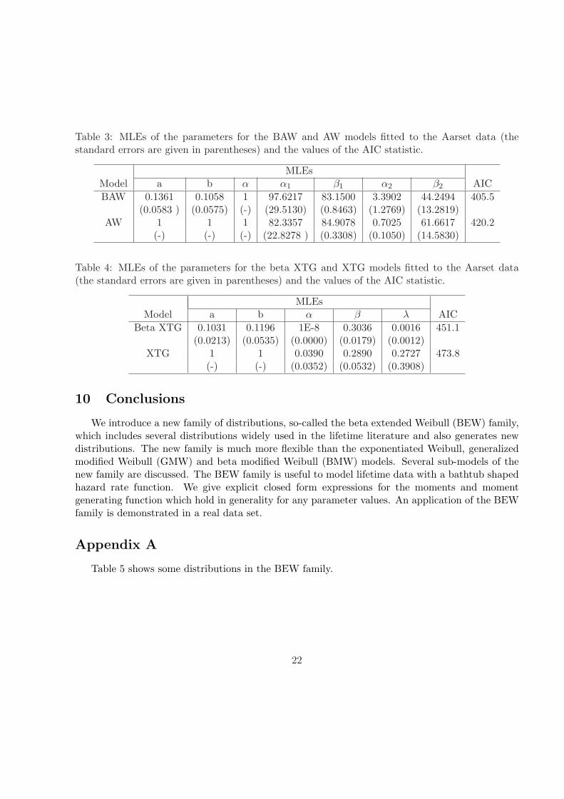
Table 3: MLEs of the parameters for the BAW and AW models fitted to the Aarset data (thestandard errors are given in parentheses) and the values of the AIC statistic.

MLEsModel a b α α1 β1 α2 β2 AICBAW 0.1361 0.1058 1 97.6217 83.1500 3.3902 44.2494 405.5

(0.0583 ) (0.0575) (-) (29.5130) (0.8463) (1.2769) (13.2819)AW 1 1 1 82.3357 84.9078 0.7025 61.6617 420.2

(-) (-) (-) (22.8278 ) (0.3308) (0.1050) (14.5830)

Table 4: MLEs of the parameters for the beta XTG and XTG models fitted to the Aarset data(the standard errors are given in parentheses) and the values of the AIC statistic.

MLEsModel a b α β λ AIC

Beta XTG 0.1031 0.1196 1E-8 0.3036 0.0016 451.1(0.0213) (0.0535) (0.0000) (0.0179) (0.0012)

XTG 1 1 0.0390 0.2890 0.2727 473.8(-) (-) (0.0352) (0.0532) (0.3908)

10 Conclusions

We introduce a new family of distributions, so-called the beta extended Weibull (BEW) family,which includes several distributions widely used in the lifetime literature and also generates newdistributions. The new family is much more flexible than the exponentiated Weibull, generalizedmodified Weibull (GMW) and beta modified Weibull (BMW) models. Several sub-models of thenew family are discussed. The BEW family is useful to model lifetime data with a bathtub shapedhazard rate function. We give explicit closed form expressions for the moments and momentgenerating function which hold in generality for any parameter values. An application of the BEWfamily is demonstrated in a real data set.

Appendix A

Table 5 shows some distributions in the BEW family.

22

Tab

le5:

Som

edi

stri

buti

ons

ofth

eB

EW

fam

ily.

Dis

trib

utio

nH

(t)

Som

esp

ecia

lsu

b-m

odel

sB

MW

tγex

p(λt)

GM

Wif

b=

1(S

ilva

etal

.,20

09)

γ≥

0,λ≥

0M

Wif

a=

b=

1B

eta

expo

nent

ial

exp

[ (λt)

α1] −

1ex

pone

ntia

lpo

wer

ifa

=b

=1

pow

er(n

ew)

α=

1,α

1,λ

>0

(Sm

ith

and

Bai

n,19

75)

Bet

aC

hen

(new

)ex

p(tβ

)−

1C

hen

ifa

=b

=1

β,λ

>0

(Che

n,20

00)

Bet

aX

TG

(new

)λ[ ex

p{(

t/λ) β

} −1]

XT

Gif

a=

b=

1β

>0,

λ>

0M

urth

yet

al.

(200

4)if

a=

b=

λ=

1B

eta

Che

nif

λ=

1C

hen

ifa

=b

=λ

=1

Bet

alo

g-W

eibu

ll(n

ew)

exp

[ (t−

µ)/

σ]

log-

Wei

bull

a=

b=

1α

=1,−∞

<µ

<∞

,σ

>0

Bet

aP

hani

(new

)(t−

µ)β

2/(σ−

t)β1

Bet

aK

ies

ifβ

1=

β2

=β

0<

µ<

t<

σ<∞

Pha

niif

a=

b=

1(P

hani

,19

87)

Kie

sif

β1

=β

2=

β,a

=b

=1

(Kie

s,19

58)

BAW

(new

)(t

/β1)α

1+

(t/β

2)α

2ad

diti

veW

eibu

llif

α=

a=

b=

1α

1,α

2,β

1,β

2>

0B

eta

gene

raliz

ed[ 1

+(t

/β)α

1] θ−

1ge

nera

lized

pow

erW

eibu

llif

a=

b=

1po

wer

Wei

bull

(new

)α

=1,

θ≥

0,α

1,β

>0

(Nik

ulin

and

Hag

high

i,20

06)

Bet

aB

LZ

(new

)ex

p(α

1t−

β/t

)B

LZ

ifa

=b

=1

α=

1,θ≥

0,α

1,β

>0

(Beb

bing

ton

etal

.,20

07)

Bet

aG

ompe

rtz

(new

)α−1 1

[ exp(

α1t)−

1]G

ompe

rtz

ifa

=b

=1

−∞<

α1

<∞

(Pha

man

dLai

,20

07)

Bet

aP

ham

(new

)a

tα1

1−

1P

ham

ifa

=b

=1

α=

1,α

1,a

1>

0(P

ham

,20

02)

Bet

atb

1[e

xp(c

td)−

1]N

adar

ajah

-Kot

zif

a=

b=

1N

adar

ajah

-Kot

z(n

ew)

b 1,c≥

0,d

>0

(Nad

araj

ahan

dK

otz,

2005

)be

taC

hen

ifb 1

=0,

c=

1B

eta

exp

[ α1+

(β/2θ

)(tθ−

t−θ)]

Slym

en-L

ache

nbru

chif

a=

b=

1Sl

ymen

-Lac

henb

ruch

(new

)α

=1,

α1,θ

>0,

(Sly

men

and

Lac

henb

ruch

,19

84)

23

Appendix B

The elements of the observed information matrix J(θ) for the parameter vetor (a, b, α, τT )T are

Jaa(θ) = −n

{Γ′′(a)Γ(a)

− ψ2(a)− Γ(a + b)[ψ′(a + b) + ψ2(a + b)

]2+ ψ2(a + b)

},

Jab(θ) = −nψ′(a + b), Jaα(θ) =n∑

i=1

uiH(ti)(1− ui)

, Jaτ (θ) = αn∑

i=1

uiH(ti)τ(1− ui)

,

Jbb(θ) = −n

{Γ′′(b)Γ(b)

− ψ2(b)− Γ(a + b)[ψ′(a + b) + ψ2(a + b)

]2+ ψ2(a + b)

},

Jbα(θ) = −n∑

i=1

H(ti), Jbτ (θ) = −αn∑

i=1

H(ti)τ ,

Jαα(θ) = − n

α2+ (a− 1)

n∑

i=1

[H(ti)

]2ui

{− 1 + ui

[1 + H(ti)

]}

(1− ui)2,

Jατ (θ) = (a + 1)n∑

i=1

uiH(ti)τ{[

1− αH(ti)](1− ui)− αuiH(ti)

}

(1− ui)2− b

n∑

i=1

H(ti)τ

and

Jττ T (θ) =n∑

i=1

h(ti)h(ti)ττ T − [h(ti)τ

]2

[h(ti)

]2 − αbn∑

i=1

H(ti)ττ T

+α(a− 1)n∑

i=1

ui

{[H(ti)ττ T − α

(H(ti)τ

)2](1− ui)− α[H(ti)τ

]2ui

}

(1− ui)2,

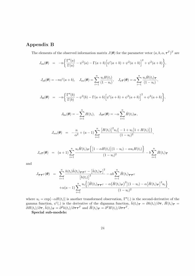
where ui = exp[−αH(ti)] is another transformed observation, Γ′′(.) is the second-derivative of thegamma function, ψ′(.) is the derivative of the digamma function, h(ti)τ = ∂h(ti)/∂τ , H(ti)τ =∂H(ti)/∂τ , h(ti)τ = ∂2h(ti)/∂ττT and H(ti)τ = ∂2H(ti)/∂ττT .

Special sub-models:

24

For the beta XTG distribution, the parameter vector is τ = (λ, β)T , and the functions h(t) andH(t) are given in Section 2. The elements of ∂2h(ti)/∂ττT and ∂2H(ti)/∂ττT are given by

h(ti)λλ =β2

λ

( tiλ

)βexp

[( tiλ

)β]{[1 +

( tiλ

)β]{β

ti

[( tiλ

)β− 1

ti

]}+

β

ti

( tiλ

)β}

,

h(ti)λβ =( ti

λ

)βexp

[( tiλ

)β]{{− 1− β log

( tiλ

)[( tiλ

)β+ 1

]}{β

ti

[( tiλ

)β+ 1

]− 1

ti

}−

β

ti

{( tiλ

)β[1 + β log

( tiλ

)]+ 1

}},

h(ti)ββ =( ti

λ

)β−1log

( tiλ

)exp

[( tiλ

)β]{1 +

[1 +

( tiλ

)β]{1 + β log

( tiλ

)[( tiλ

)β+ 1

]}

+( ti

λ

)β[1 + β log

( tiλ

)]},

H(ti)λλ = −β

λ

( tiλ

)exp

[( tiλ

)β][− 1 + β

( tiλ

)β+ β

], H(ti)λβ = (1− β)

( tiλ

)β

and

H(ti)ββ = λ( ti

λ

)β[log

( tiλ

)]2exp

[( tiλ

)β][1 +

( tiλ

)β].

For the BAW distribution, the parameter vector is τ = (α1, α2, β1, β2)T and the functions h(t)and H(t) are given in Section 2. The elements of ∂2h(ti)/∂ττT and ∂2H(ti)/∂ττT are given by

h(ti)α1α1 =1β1

( tiβ1

)α1−1log

( tiβ1

)[2 + α1 log

( tiβ1

)], h(ti)α1α2 = 0,

h(ti)α1β1 = − 1β1

( tiβ1

)α1−1{[ 1

β1+

(α1 − 1)β1

][1 + α1 log

( tiβ1

)]− α1

β1

}, h(ti)α1β2 = 0,

h(ti)α2α2 =1β2

( tiβ2

)α2−1log

( tiβ2

)[2 + α2 log

( tiβ2

)], h(ti)α2β1 = 0,

h(ti)α2β2 = − 1β2

( tiβ2

)α2−1{[ 1

β2+

(α2 − 1)β2

][1 + α2 log

( tiβ2

)]− α2

β2

},

25

h(ti)β1β1 =α1

β1

( tiβ1

)α1−1{[

− 1β1

+ log( ti

β1

)]2+

(1− β1

β21

)}, h(ti)β1β2 = 0,

h(ti)β2β2 =α2

β2

( tiβ2

)α2−1{[

− 1β2

+ log( ti

β2

)]2+

(1− β2

β22

)},

H(ti)α1α1 =( ti

β1

)α1[log

( tiβ1

)]2, H(ti)α1α2 = 0,

H(ti)α1β1 = − 1β1

( tiβ1

)α1

log( ti

β1

)[α1 log

( tiβ1

)+ 2

], H(ti)α1β2 = 0,

H(ti)α2α2 =( ti

β2

)α2[log

( tiβ2

)]2, H(ti)α2β1 = 0,

H(ti)α2β2 = − 1β2

( tiβ2

)α2

log( ti

β2

)α2

[log

( tiβ2

)+ 2

],

H(ti)β1β1 =α1

β1

( tiβ1

)α1(1 + α1

β1

), H(ti)β1β2 = 0

and

H(ti)β2β2 =α2

β2

( tiβ2

)α2(1 + α2

β2

).

References

Aarset, M. V. (1987). How to identify bathtub hazard rate. IEEE Transactions Reliability, 36,106-108.

Bebbington, M., Lai, C. D. and Zitikis, R. (2007). A flexible Weibull extension. ReliabilityEngineering and System Safety, 92, 719-726.

Brown, B.W., Floyd, M. S. and Levy, L.B. (2002). The log F: a distribution for all seasons.Computational Statistics, 17, 47-58.

Carrasco, J. M. F., Ortega, E. M. M. and Cordeiro, G. M. (2008). A generalized modified Weibulldistribution for lifetime modeling. Computational Statistics and Data Analysis, 53, 450-462.

26

Chen Z. A. (2000). A new two-parameter lifetime distribution with bathtub shape or increasingfailure rate function. Statistics and Probability Letters, 49, 155-61.

Cordeiro, G. M., Nadarajah, S., and Ortega, E. M. M. (2009). General results for beta Weibulldistribution. Submitted to Technometrics.

Doornik, J. (2007). Ox 5: Object-oriented matrix programming language. 5th ed. London:Timberlake Consultants.

Eugene, N., Lee, C. and Famoye, F. (2002). Beta-normal distribution and its applications. Com-munication in Statistics - Theory and Methods, 31, 497-512.

Gupta, R. D. and Kundu, D. (1999). Generalized exponential distributions. Australian and NewZealand Journal os Statistics, 41, 173-188.

Gupta, R. D. and Kundu, D. (2001). Exponentiated exponential distribution: an alternative togamma and Weibull distributions. Biometrical Journal, 43, 117-130.

Gupta, A. K. and Nadarajah, S. (2004). Handbook of Beta Distribution and Its Applications. NewYork: Marcel Dekker.

Gurvich, M. R., Dibenedetto, A. T. and Ranade, S. V. (1997). A new statistical distribution forcharacterizing the random strength of brittle materials. Journal of Materials Science, 32,2559-2564.

Hosking, J.R.M., (1986). The theory of probability weighted moments. Research Report RC12210,New York: IBM Thomas J. Watson Research Center.

Jones, M. C. (2004). Family of distributions arising from distribution of order statistics. Test, 13,1-43.

Kies, J. A. (1958). The Strength of Glass. Naval Research Laboratory, Washington DC, ReportNo 5093.

Kundu, D. and Rakab, M. Z. (2005). Generalized Rayleigh distribution: different methods ofestimation. Computational Statistics and Data Analysis, 49, 187-200.

Lai, C. D., Xie, M. and Murthy, D. N. P. (2003). A modified Weibull distribution. Transactionson Reliability, 52, 33-37.

Lawless, J. F. (2003). Statistical Models and Methods for Lifetime Data. 2nd ed. Wiley: NewYork.

Mudholkar, G. S. and Srivastava, D. K. (1993). Exponentiated Weibull family for analyzingbathtub failure-real data. IEEE Transaction on Reliability, 42, 299-302.

27

Mudholkar, G. S., Srivastava, D. K. and Friemer, M. (1995). The exponentiated Weibull family:A reanalysis of the bus-motor-failure data. Technometrics, 37, 436-445.

Mudholkar, G. S., Srivastava, D. K. and Kollia, G. D. (1996). A generalization of the Weibulldistribution with application to the analysis of survival data. Journal of American StatisticalAssociation, 91, 1575-1583.

Murthy, D. N. P., Xie, M. and Jiang, R. (2004). Weibull Models. New York: John Wiley andSons.

Nadarajah, S. (2005). On the moments of the modified Weibull distribution. Reliability Engineer-ing and System Safety, 90, 114-117.

Nadarajah, S. and Gupta, A. K. (2004). The beta Frechet distribution. Far East Journal ofTheoretical Statistics, 14, 15-24.

Nadarajah, S. and Kotz, S. (2004). The beta Gumbel distribution. Mathematical Problems inEngineering, 10, 323-332.

Nadarajah, S. and Kotz, S. (2005). On some recent modifications of Weibull distribution. IEEETransaction on Reliability, 54, 561-562.

Nadarajah, S. and Kotz, S. (2006). The beta exponential distribution. Reliability Engineeringand System Safety, 91, 689-697.

Nikulin, M. and Haghighi, F. (2006). A Chi-squared test for the generalized power Weibull familyfor the head-and-neck cancer censored data. Journal of Mathematical Sciences, 133, 1333-1341.

Pham, H. (2002). A vtub-shaped hazard rate function with applications to system safety. Inter-national Journal of Reliability and Applications, 3, 1-16.

Pham, H. and Lai, C. D. (2007). On recent generalizations of the Weibull distribution. IEEETransactions on Reliability, 56, 454-458.

Phani, K. K. (1987). A new modified Weibull distribution. Communications of the AmericanCeramic Society, 70, 182-184.

Prudnikov, A. P., Brychkov, Yu. A., Marichev, O. I. (1986). Integral and Series: ElementaryFunctions, v.1, Gordon and Breach Science: New York.

SAS Institute. SAS/STAT User´s Guide: Version 9. Cary: SAS Institute. 2004. 5121 p.

Silva, G.O., Ortega, E. M. M. and Cordeiro, G. M. (2009). The beta modified Weibull distribution.Submitted to Lifetime Data Analysis.

28

Slymen, D. J. and Lachenbruch, P. A. (1984). Survival distributions arising from two familiesand generated by transformations. Communications in Statistics-Theory and Methods, 13,1179-1201.

Smith, R.M. and Bain, L.J. (1975). An exponential power life testing distributions. Communica-tions in Statistics, 4, 469-481.

Xie, M. and Lai, C. D. (1995). Reliability analysis using an additive Weibull model with bathtub-shaped failure rate function. Reliability Engineering and System Safety, 52, 87-93.

Xie, M., Tang, Y. and Goh, T. N. (2002). A modified Weibull extension with bathtub failure ratefunction. Reliability Engineering and System Safety, 76, 279-285.

Wang, F. K. (2000). A new model with bathtub-shaped failure rate using an additive Burr XIIdistribution. Reliability Engineering and System Safety, 70, 305-312.

White, J. S. (1969). The Moments of Log-Weibull Order Statistics. Technometrics, 11, 373-386.

29