Corresponding author:Lamya A. Baharith,

THE BETA GENERALIZED INVERSE

WEIBULL DISTRIBUTION

Lamya A. Baharith1*, Salwa A Mousa2 , Mahmoud A. Atallah3, Sohaila H.

Elgayar4

1Department of Statistics, Faculty of Science, King Abdulaziz University, Jeddah, SaudiArabia

P.O.Box 42805 Jeddah 21551

2Department of Statistics, Faculty of Science, King Abdulaziz University, Jeddah, SaudiArabia

P.O.Box 42805 Jeddah 21551,Permanent Address: Faculty of Commerce (Girls Campus), Al-Azhar University, Nasr city, Cairo, Egypt.

3Department of Statistics, Faculty of Science, King Abdulaziz University, Jeddah, SaudiArabia, Permanent Address: Faculty of Engineering, Ain Shams University, Cairo, Egypt.

P.O.Box 80203 Jeddah 21589

4Department of Statistics, Faculty of Science, King Abdulaziz University, Jeddah, SaudiArabia

P.O.Box 42805 Jeddah 21551, Permanent Address: Institute of Statistical Studies andResearch (ISSR), Cairo University, Egypt.

ABSTRACTThe beta generalized inverse Weibull distribution (BGIW) is suggested in this paper. Themathematical properties of the BGIW distribution are provided and the expression for themoment generating function is derived. Also, the analytical shapes of the correspondingprobability density function, reliability function, hazard rate function, and mode are derivedwith graphical illustrations. Expressions for the r -th positive and negative moments arecalculated and the variation of the skewness and kurtosis measures is investigated. Momentand likelihood estimators of the parameters are derived. The observed information matrix isobtained. Simulation study is carried out to investigate the performance of the maximumlikelihood method of estimation. Moreover, analysis of real data set is conducted todemonstrate the usefulness of the proposed distribution.

Keywords:Beta generalized inverse Weibull distribution, Fisher information matrix, momentgenerating function, moment estimation, maximum likelihood estimation.

1. INTRODUCTIONThe inverse Weibull distribution (IW) usually used in reliability and biological studies. Thethree-parameter generalized inverse Weibull (GIW) distribution, which extends to severaldistributions, and commonly used in the lifetime-literature, is more flexible than the inverseWeibull distribution. Mudholkar et al. [1], Jiang et al. [2] and De Gusmao et al. [3] haveintroduced and discussed the three-parameter GIW distribution.

Let T be a random variable from GIW distribution, so the cumulative distribution function(cdf) of T is defined as

( ; , , ) , 0.tG t e t (1)

Therefore, the probability density function pdf of the GIW distribution with three parameters (0 , 0 , 0 ) is given by

( 1)( ; , , ) , 0.tg t tt e (2)

Recent developments focus on new techniques to construct useful distributions. Theseinclude the approach explored by Eugene et al. [4] and Jones [5]. The new technique ismotivated by the following general class:If ( )G is the cdf of a random variable, then a generalized class of distributions can bedefined by

( )( ) ( , ),G xF x I a b x , (3)

where,( )

( ) 1 1( ) ( )

0

( , ) ( ) ( )( , ) , ( , ) (1 ) , ( , ) ,( , ( , )

G xG x a b

G x G x

B a b a bI a b B a b z z d z B a bB a b a b

and ( ) denotes the incomplete beta function ratio, the incomplete beta function, the betafunction, and the gamma function, respectively. The beta density has different type ofshapes. The beta density is symmetric ifa = b = 1, is unimodal when a, b>1 and “U” shapedwhen a, b< 1. It has positively skewed when a<b and negatively skewed when b .

The pdf of this general class of distributions namely the Beta Type I distribution is defined by

1 11( ; , ) (1 ) , 0 1( , )

a bf u a b u u uB a b

(4)

Recently, this class of generalized distributions has gained more attention from manyresearches. Eugene et al. [4] have constructed the beta normal distribution by substituting

( )G in (3) to be the cdf of the normal distribution with parameters μ and σ. Jones [5] focusedon cases where ( )G is symmetric about zero with location and scale parameters. Moreover,beta distributions have been studied by NadarajahandKotz[6,7]. They have proposed thebeta Gumbel distribution by substituting ( )G in (3) to be the cdf of the Gumbel distributionwith parameters μ and σ. Beta distributions have been studied also by Akinsete et al. [8],ZografosandBalakrishnan[9]. Beta-Weibull distribution was first introduced by Famoye et.al.[10]. Properties of the beta Weibull model were studied by Lee et al. [11]. Cordeiro et al. [12]has provided an expansion for the cumulative distribution function, the moments, and themoment generating function of the beta Weibull distribution. Moreover, maximum likelihoodestimation and formulas for the elements of the Fisher information matrix were provided.Barreto-Souza et al. [13] introduced the beta generalized exponential distribution andprovided comprehensive mathematical properties of this distribution. They obtained thedensity, moment generating function and r-th moment of the order statistics. Cordeiro et al.[14] introduced the beta exponentiatedWeibull distribution; they provided the moments andtwo expressions for the moment generating function of the new distribution.

In this paper, a new beta distribution is introduced by taking ( )G to be the generalizedinverse Weibull distribution and will refer to it as beta generalized inverse Weibull distribution(BGIW). The inverse Weibull distribution is a special case of (2) when θ = 1 and representsa particular case of the BGIW distribution when θ = a = b =1.

The rest of the paper is organized as follows: Section 2 provides the cumulative distribution,probability density, reliability, and hazard functions of the BGIW distribution with graphicalillustrations. Some special models of BGIW are studied in Section 3. Theoretical propertiesare discussed in Section 4. In Section 5, the parameters estimation are obtained by themethod of moment and maximum likelihood method in addition to presenting thesamplinginformation matrix. The performance of the estimators is investigated throughsimulation study in Section 6. Section 7 presents the analyses of real data set to illustratethe usefulness of the proposed distribution. Finally, some concluding remarks are presentedin Section 8.

2. THE BETA GENERALIZED INVERSE WEIBULL DISTRIBUTIONThe cdf of the BGIW distribution can be obtained as follows:

( )1 1

( )0

1( ) ( , ) (1 ) , 0 1, , 0.( , )

G xa b

G tF t I a b z z d z z a bB a b

(5)

Substituting equation (1) into equation(5) yields

e ( ) 1 1

0

xp1( ) (1 ) , 0 1, , 0.( , )

t a bF t z z d z z a bB a b

(6)

Property 2.1 Probability density function of BGIW distributionDifferentiating both sides of (6) with respect to t, the explicit form of the pdf of the BGIWdistribution can be obtained as:

1( ) ( )1( ) ( ) 1 , 0, , , , , 0

( , )t t

ba a

tf t e e t a bB a b

(7)

For non-integer positive value b> 0, (7) can be rewritten as an infinite power series in theform

( ) ( )1

0

( 1)( ) ( ) , 0, , , , , 0, .( , ) ( , 1)

t

ja j

tj

f t e t a b b jb B a b B b j j

(8)

Throughout the paper, this distribution will be referred to as the beta generalized inverseWeibull distribution BGIW(α, β, θ, a, b). The density given by (8) is a proper density andwhena = b = 1, it reduces to the generalized inverse Weibull density with scale parameter αand the two shape parameters, β and θ. This model is constructed based on the beta andthe generalized inverse Weibull distributions.

Property 2.2 Cumulative distribution function of BGIW distributionFrom (8) the corresponding cdfcan be written as:

( ) ( )

0

1 ( 1)( ) , 0, , , , , 0.( , ) ( , 1) ( )

t

ja j

jF t e t a b

b B a b B b j j a j

(9)

Property 2.3 Reliability function of BGIW distributionThe reliability function of the BGIW (α, β, θ, a, b) distribution can be written as

( ) ( )

0

1 ( 1)( ) 1 , 0, , , , , 0.( , ) ( , 1)

t

ja j

jR t e t a b

b B a b B b j j

(10)

Property 2.4 Hazard function of BGIW distributionThe hazard function of the BGIW (α, β, θ, a, b) distribution can be written in the form:

( ) ( )1

0

( ) ( )

0

( 1)( )( , ) ( , 1)

( ) , 0, , , , , 0, .1 ( 1)1( , ) ( , 1)

t

t

ja j

tj

ja j

j

eb B a b B b j j

h t t a b b je

b B a b B b j j

(11)

Remark 2.1 The index j in (8) – (11) stops at (b-1), when b> 0 is a positive integer.

Graphical representation of the pdf and reliability function for selected values of α, β, θ, a,and b are given in Figures 1 and 2, respectively. It indicates the stability of thecharacteristics of the initial distribution GIW after adding the new parameters aandb.

Fig.1. Plots of the BGIW density function. α=2, β =2.5, θ =2.5, (I): a =0.5, b=0.5, (II): a = 2,b=0.5. (III): a =0.5, b=4. (IV): a =5 , b=5 (V) :a =6 , b= 3 (VI): a =3, b=5.

Fig.2. Plots of the BGIW reliability function. α=2, β =2.5, θ =2.5, (I): a =0.5, b=0.5, (II): a = 2,b=0.5. (III): a =0.5, b=4. (IV): a =5 , b=5 (V) :a =6 , b= 3 (VI): a =3, b=5.

Furthermore, Figure 3 illustrates different shapes of the failure rate function of the BGIWdistribution which take monotonically decreasing case ( III) and upside down bathtub shapescases (I) , (II) and (IV).

Fig.3. Plots of the BGIW hazard rate functions. (I) α = 4, β = 2, θ =1.5, a = 1.5, b = 1.3, (II) α =10, β= 2, θ =1.2, a = 1.1, b = 1.1, (III) α = 5, β = 0.2, θ = 0.2, a = 12, b = 5, (IV) α = 2, β = 2.5 ,θ =2.5, a=0.5, b = 0.5

3. SPECIAL MODELSThe BGIW distribution in equation (7) represents a generalization of several distributionsthat have been considered in the literature. In particular, BGIW distribution becomesgeneralized inverse Weibull GIW (α, β, θ) distribution when a = b =1. The beta inverseWeibull BIW (α, β, a, b) distribution is clearly a special case of BGIW distribution when θ =1.In addition, the generalized inverse exponential distribution GIE (η, θ) is a special case ofBGIW distribution whenβ = a = b =1 and 1a .Inverse Weibull IW (α, β) distribution canbe obtained from (7) by making θ = a = b = 1. The BGIW distribution contains the inverseexponential IE (α), and inverse Rayleigh IR (η) distributions as special models for θ = β = a= b=1, and β = 2, θ = a = b = 1, 2 , respectively. These special models with theirreferences are summarized in Table 1 and graphically represented in Figure 4.

Furthermore, the BGIW distribution in (7) is a general form of several new beta distributions.The beta inverse exponential distribution BIE (α, a, b) is clearly a special case of BGIWwhen θ = β =1. When β =1, the beta generalized inverse exponential distribution BGIE (η,θ, a, b) can be obtained. The BGIW distribution can be reduced to the beta inverse Rayleighdistribution BIR (η, a, b) when θ = 1, β = 2, 2 and to the beta generalized inverseRayleigh distribution BGIR (η, θ, a, b) when β = 2, 2 .

Table 1. Generalized inverse Weibull type distributions

Distribution BGIW (α, β, θ,a, b) Main reference

α θ β a b

GIW (α, β, θ) α θ β 1 1 De Gusmao et al. [3]

BIW (α, β, a, b) α 1 β a b Khan [15]

GIE (η,θ) 1η α θ 1 1 1 Khan [16]

IW (α, β) α 1 β 1 1 Keller and Kamath [17]

IE (α) α 1 1 1 1 Keller and Kamath [17]

IR (η) η = α2 1 2 1 1 Voda [18]

B ≡ Beta, E ≡ exponential, G ≡ generalized, I ≡ inverse, R ≡ Rayleigh, W ≡ Weibull

Fig.4. Plots the BGIW probability density functions of the six special models

4. STATISTICAL PROPERTIESIn this section, some of the basic statistical properties of the BGIW distribution are provided.

Property 4.1 Quantile function, median, and simulationThe quantile function of BGIW (α, β, θ, a, b) distribution corresponding to (7) is

1/1 11( ) ( ) log{ ( , )} ,ut Q u F u I a b

(12)

where 1( , )uI a b denotes the inverse of the incomplete beta function with parameters a and b.The quartiles Q1, Q2 (median), and Q3 of the BGIW (α, β, θ, a, b) distribution correspond tothe values u = 0.25, 0.50, and 0.75 respectively.The simulation of the BGIW (α, β, θ, a, b) random variable T is easily obtained if B is arandom number following a beta distribution with parameters a andb then 1/1 log ,t B

follows a BGIW (α, β, θ, a, b) distribution.

Property 4.2 Mode of the BGIW distributionThe BGIW (α, β, θ a, b) distribution is unimodal. The mode is located at ( ) 0f t .Equivalently, it is the solution of the equation (log ( )) 0f t . That is

( )( 1) ( 1) 0.tt t a b e a (13)

The mode of BGIW distribution is obtained numerically at some selected values ofparameters aandb when α =2, β = 2.5, θ = 2.5. Table 2 shows that the mode valuesapproximately coincide with the graphical mode shown in Figure 1 for all selected values ofparameters.

Table 2. Numerical evaluation of the mode of BGIW for each case in Figure1

Parameters a = b= 0.5 a=0.5, b = 4 a = 2, b = 0.5

Mode 1.97 ( I ) 1.75 ( III ) 3.78 ( II )

Parameters a = b = 5 a = 6, b = 3 a = 3, b= 5

Mode 3.15 ( IV ) 3.83 ( V ) 2.71 ( VI )

Property 4.3 The non-central moments of the BGIW distributionThe r-th non-central moment of the BGIW (α, β, θ, a, b) distribution can be written as

/

(1 )

0

( 1)1 ( ) , , 1,2,...( , ) ( , 1)

rr r jr

rj

a j r rb B a b B b j j

(14)

Proof.Using equation (8) and substituting ( )w t , we obtain

( ) ( )1

0 0

( 1) ( )( , ) ( , 1) i

t

ja jr

r tj

t e dtbB a b B b j j

1/ ( )

0 0

1 ( 1) [ ( ) ]( , ) ( , 1)

jr a j ww

je dw

bB a b B b j j

// ( )

0 0

( 1)( , ) ( , 1)

r r jr a j w

jw e dw

b B a b B b j j

/(1 )

0

( 1)(1 ) ( ) , , 1,2,...( , ) ( , 1)

rr r jr

rj

a j r rbB a b B b j j

Therefore, the mean and the variance of the BGIW (α, β, θ, a, b) distribution are

11/

(1 )1

0

( 1)(1 ) ( ) , 1,( , ) ( , 1)

j

ja j

bB a b B b j j

(15)

22 2/

(1 )2 22

0

( 1)(1 ) ( ) , 2.( , ) ( , 1)

j

ja j

bB a b B b j j

(16)

Property 4.4 The central moments of the BGIW distributionThe r-th central moment of the BGIW (α, β, θ, a, b) distribution is given by

0[( ) ] ( )( 1)

rr r k k

r k r kk

M E X

. (17)

The coefficient of skewness 3/23 3 2/M M , the coefficient of kurtosis 2

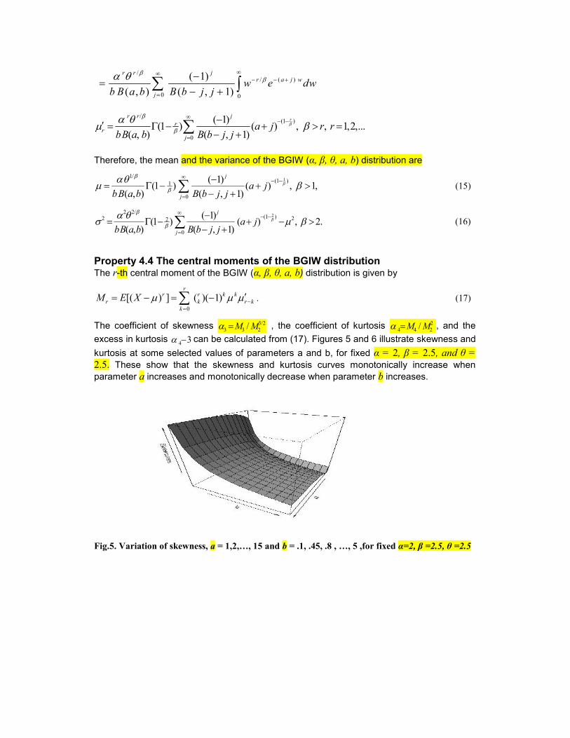
4 4 2/M M , and theexcess in kurtosis 4 3 can be calculated from (17). Figures 5 and 6 illustrate skewness andkurtosis at some selected values of parameters a and b, for fixed α = 2, β = 2.5, and θ =2.5. These show that the skewness and kurtosis curves monotonically increase whenparameter a increases and monotonically decrease when parameter b increases.

Fig.5. Variation of skewness, a = 1,2,…, 15 and b = .1, .45, .8 , …, 5 ,for fixed α=2, β =2.5, θ =2.5

Fig.6. Variation of kurtosis, a = 1,2,…, 15 and b = .1, .45, .8 , …, 5 ,for fixed α=2, β =2.5, θ =2.5

Property 4.5 Negative moments of the BGIW distributionThe r-th non-central negative integral moment of the BGIW (α, β, θ, a, b) distribution is givenby

( ) ( )1

0 0

( 1) ( )( , ) ( , 1)

t

i

ja jr

r tj

t e dtbB a b B b j j

. (18)

After some manipulations, Equation (18) reduces to/

( 1)

0

( 1)( 1) ( ) , , 1,2,...( , ) ( , 1)

rr r jr

rj

a j r rbB a b B b j j

(19)

Property 4.6 Moment generating function of the BGIW distributionThe moment generating function of the BGIW (α, β, θ,a, b) distribution can be expressed as

/(1 )

0 0

( 1)( ) (1 ) ( ) , ,( , ) ! ( , 1)

kk k k jk

Tk j

uM u a j kbB a b k B b j j

(20)

Proof.

0

( ) ( )tuTM u e f t dt

.

Using ( )f t from equation (8) and expanding the function t xe into powers of t, we get

0( )

!

k

T kk

uM uk

.

Substituting equation (14) into the last equation, equation (20) follows directly.

The k-th non-central moment follows from equation (20), as the coefficient of !ku k in thepower series expansion of ( )TM u into powers of u.

5.PARAMETER ESTIMATIONIn this section, the five parameters of BGIW distribution will be estimated using the methodof moments and the method of maximum likelihood.

5.1. Moments method of estimationIn order to estimate of the parameters α, β, θ, a, b of BGIW distribution based on the methodof moment, where the first 5 non-central population moments ( , 1,  2,   ,  5r r ) areequated to the first 5 non-central sample moments ( , 1,2,...,5rm r ). That is

,  r 1,  2,   ,  5r rm .

The resulting equations are:/

(1 )

0 0

( 1) 1(1 ) ( ) , , 1,2,...5( , ) ( , 1)

rr r j nrri

j ia j t r r

nb B a b B b j j

. (21)

Because of the complexity of the existing equations, it is difficult to obtain a closed formanalytic solution of the system in equation(21). Therefore a suitable numerical technique canbe used to obtain the required moment estimates of the parameters α, β, θ, a, and b.

5.2.Maximum likelihood methodSuppose that 1 2, , , nt t t are the n lifetimes observed arising from ( )f t defined in equation

(8). The likelihood function 1( ) ( , , , , ) [ ( ; )], ( , , , , )nj iL v L a b f t v v a b is given

by

1

1( ) ( )

1 1

1

( ) 1( , )

n

ti ti i

n n n bna

nn i

ii

L v e et B a b

. (22)

It is usually easier to maximize the natural logarithm of the likelihood function. So, thenatural logarithm of the likelihood function can written as

1

( )

1 1

log log log log log ( , ) ( 1) log

( ) ( 1) log 1 .ti

i

n

ii

n n

ti i

L n n n n B a b t

a b e

(23)

The maximum likelihood estimates, ˆˆ  ˆˆ ˆ, ,,,v a b , are obtained by taking the first

derivative of the natural logarithm of the likelihood function with respect to ,  ,  ,  ,  a b andequating to zero as followsThe maximum likelihood estimates, ( , , , , )v a b

, are obtained by taking the firstderivative of the natural logarithm of the likelihood function with respect to , , , , andequating to zerousing the notation exp[ ( ) ]i it

as follows

1 1 11 1

1 1

log ( ) ( 1) ( ) (1 )i i

n n

i it ti i

L n a b

,

1

1 1 1

log log log ( ) log( ) ( 1) ( ) log( ) (1 )i i i i

n n n

i i it t t ti i i

L nn t a b

,

1

1 1

log ( ) ( 1) ( ) (1 )i i

n n

i it ti i

L n a b

,

1

log ( ) ( ) ( )i

n

ti

L n a n a ba

,

1

log ( ) ( ) log(1 )n

ii

L n b n a bb

, (24)

Here, ( )x is the digamma function defined as follows

( )( ) [log ( )]( )

d xx xdx x

.

Setting these 5 expressions in equation (24) to zero and solving the resulting system of non-linear equations to obtain the maximum likelihood estimators of the unknown parameters,α, β, θ, a and bof BGIW distribution.

5.3. Asymptotic confidence boundsSince the MLE’s of the vector v of unknown parameters are not obtained in closed forms,then it is not possible to derive the exact distributions of the MLE’s v . The observedinformation matrix is obtained for approximate confidence intervals and hypothesis tests ofthe vector v . This is because the expected information matrix of α, β, θ, a, and b involvenumerical integration. The observed 5X5 information matrix I is:

,

a b

a b

a b

a a a a ab

b b b b a bb

I I I I II I I I II I I I III I I I II I I I I

where2 log , , 1,...,5

i jv vi j

LI i jv v

which are given in the Appendix.

The asymptotic distribution of ( )n v v is 15 (0, )N I , that can be used to create

approximate intervals and confidence regions for the parameters and for the hazard and thesurvival functions. Asymptotic confidence bounds with significance level for each

parameter iv is given by ,/2

i iiv Z v , where ,i iv is the i-th diagonal element of 1I for

1,...,5i and /2Z is the (1 2) percentile of the standard normal distribution, see Bainand Engelhard [19].

6. SIMULATION STUDYMonte Carlo simulation study is performed to investigate the maximum likelihood estimators(MLE's)and studiedthem with respect to their relative absolute bias (RAB) and relative meansquared error (RMSE).The relative absolute bias of the estimate jv is defined as

( )( ) , 1,...,5ii

j

Bias vRAB v jv

.

The relative mean squared error of the estimate jv is defined as

( )( ) , 1,...,5ii

j

MSE vRMSE v jv

,

where jv denotes the estimate of jv .All computations are performed using R package.

6.1. Numerical results for the maximum likelihood estimatesMLE of α, β, θ, a, and bis obtained by solving nonlinear equations which are given inequation (24) simultaneously, using nlminb routine in Rwhich uses variants ofthe Newton-Raphson algorithm. Then, the performances of the MLE’s are studied mainly for differentsample sizes (n = 10, 20, 30, 40, 50) and given values of the parameters α= 3, β= θ = a =2.5 and b= 2.4. Repeat each computation over 10000 replications for different cases. It isobservedfrom Table 3that the RAB and RMSE decrease as the sample size increases.

Table 3. Numerical evaluation of maximum likelihood estimates of the5parameterBGIWdistribution

n Parameters α=3 β=2.5 θ=2.5 a=2.5 b=2.4

10

MLE 4.713 2.659 2.662 2.658 2.648

RAB 0.571 0.064 0.063 0.063 0.103

RMSE 1.299 0.129 0.133 0.131 0.150

20

MLE 4.569 2.580 2.571 2.573 2.575

RAB 0.523 0.032 0.029 0.029 0.073

RMSE 0.957 0.055 0.053 0.053 0.064

30

MLE 4.522 2.548 2.546 2.544 2.544

RAB 0.507 0.019 0.018 0.017 0.060

RMSE 0.858 0.033 0.033 0.032 0.041

40

MLE 4.499 2.533 2.533 2.539 2.535

RAB 0.500 0.013 0.013 0.015 0.056

RMSE 0.811 0.024 0.023 0.024 0.031

50 MLE 4.485 2.526 2.530 2.526 2.526

RAB 0.495 0.010 0.012 0.010 0.053

RMSE 0.783 0.018 0.018 0.019 0.026

7. APPLICATIONIn this section, the utility use of the BIGW distribution may be demonstrated by using a dataset. The data set of breaking strengths of carbon fibbers from sample size 57 and length 1 isused to fit the BGIW by the method of maximum likelihood, see Lawless [20].

The Kolmogorov-Smirnov (K.S.) goodness-of-fit test is K.S.= 0.1053 and the correspondingP= 0.91, which indicate that the BGIW model can be used to analyze this data set.Also, the K.S.test is used to verify the fitted of the cumulative distribution function of MLEand the empirical distribution function are displayed in Figure 7.

Fig. 7. Estimated cumulative function and the empirical for breaking strength of single carbonfibbers of length 1

The maximum likelihood estimates of the parameters with relative mean square error andthe Akaike information criterion (AIC) for the fitted models are illustrated in Table 4. It can beseen from the Table 4 that the AIC criteria’s measures for the BGIW and the BIW distributionare numerically similar. However, the beta generalization of BIW, provided by the BGIW,remains an overall better approach for the MLE, as the two extra parameters a andb areinvolved. Therefore, it can be concluded that the BIGW (as far as the AIC criteria’s measureis concerned), is the more appropriate distribution than the other three sub models.

Table 4. MLE’s of the model parameters for the breaking strength of single carbonfibbers data,the relative mean square error (in brackets) and the AIC criteria’s measure.

8. CONCLUDING REMARKSThe beta generalized inverse Weibull distribution is proposed. This generalizes the betainverse Weibulldistribution discussed by Khan [15] and represents a generalization of otherseveral models previously studied in the literature. The general mathematical properties ofthis distribution are studied. The moment generating function is derived and infinite sums forthe moments of BGIW distribution are provided. The ML estimators and moment estimatorsof the BGIW parameters are obtained. The information matrix and the asymptotic confidencebounds of the parameters are derived. Monte Carlo simulation studies were carried outunder different sample sizes to study the theoretical performances of the MLE of theparameters. Real data set was analyzed and the BIGW has provide a good fit for the dataand was more appropriate model compared to the GIW,BIW, and IW sub-models.

ACKNOWLEDGEMENTSThe authors would like to thank the referees and the Guest editors forcarefully reading thepaper and for their help in improving the paper.

COMPETING INTRESTSAuthors have declared that no competing interests exist.

AUTHORS CONTRIBUTIONSAll authors contributed equally and significantly to this research work. All authors read andapproved the final manuscript.

Distribution α θ β a b AIC

BGIW2.479

(0.115)

2.693

(0.036)

2.708

(0.028)

2.987

(0.110)

3.00101

( 0.105)

160.699

GIW2.99404

(0.494)

2.15517

(0.025)

2.977

(0.000176)

1

(-)

1

(-)

181.25

BIW3.0010

(0.501)

1

(-)

2.968668

(0.00045)

3.988

(0.0714)

2.232

(0.027)

161.3827

IW2.989

(0.489)

1

(-)

3.0011

(4.03 e-7)

1

(-)

1

(-)

205.742

REFERENCES1. Mudholkar GS, Srivastava DK and Kollia GD. A generalization of the Weibull

distribution with application to the analysis of survival data. J Americ Statist Assoc.1996;91:1575-1583.

2. Jiang R, Murthy DNP. and JIP. Models involving two inverse Weibull distributions.Reliability Engineering and System Safety. 2001;1(73):73-81.

3. De Gusmao FRS, Ortega EMM, and Cordeiro GM. The generalized inverse Weibulldistribution. Stat Papers. 2011;3(52):591-619.

4. Eugene N, Lee C, and Famoye F. Beta normal distribution and its applications.CommunStatist – Theory and Methods. 2002;4(31):497-512.

5. Jones MC. Families of distributions arising from distributions of order statistics. Test.2004;13(1):1-43.

6. Nadarajah S and Kotz S. The beta Gumbel distribution. Math Probab Eng. 2004;4:323-332.

7. Nadarajah S and Kotz S. The beta exponential distribution. Reliability Engineering andSystem Safety. 2006;6(91):689-697.

8. Akinsete A, Famoye F, and Lee C. The beta-Pareto distributions. Statistics.2008;6(42):547-563.

9. Zografos K and Balakrishnan N. On families of beta- and generalized gammagenerated distributions and associated inference. Statistical Methodology. 2009; 6:344-362.

10. FamoyeF, Lee C, and Olumolade O. The beta -Weibull distribution. J Statistical Theoryand Applications. 2005; 4(2):121-136

11. Lee C, Famoye F, and Olumolade O. The beta-Weibull distribution: Some propertiesand applications censored data. J Modern Applied Statistical Method. 2007;6(1):173-186.

12. Cordeiro GM, Simas AB, and Stosic BD. Explicit expressions for the moments of thebeta Weibull distribution. J Statist ComputSimul. 2008;1:1-17.

13. Barreto-Souza W, Santos AHS, and Cordeiro GM. The beta generalized exponentialdistribution. J Statist ComputSimul. 2010;2(80):159-172.

14. Cordeiro GM, Gomes AE, da-Silva CQ, and OrtegaEMM. The betaexponentiatedWeibull distribution. Journal of Statistical Computation and Simulation.2013;1(83):114-138.

15. Khan MS. The Beta Inverse Weibull Distribution. International Transactions inMathematical Sciences and Computer. 2010;1(3):113-119.

16. Khan MS. Theoretical Analysis of Inverse Generalized Exponential Models. Inproceeding of the 2009 International Conference on Machine Learning and Computing(ICMLC 2009), Perth, Australia. 2011;(20):18-24.

17. Keller AZ, and Kamath ARR. Reliability Analysis of CNC Machine Tools. ReliabilityEngineering. 1982;6(3):449-473.

18. Vodă VG. On the Inverse Rayleigh Distribution Random Variable. Rep StatisticalApplied Research JUSE. 1972;4(19):13-21.

19. Bain L. J. and Engelhardt M. Introduction to Probability and Mathematical Statistics.2nd ed: Boston: Duxbury Press; 1992.

20. Lawless JF. Statistical Models and Methods for Life Time Data. 2nd ed. New York:Wiley; 2003.

APPENDIXThe elements of the observed 5X5 information matrix I are given by

22 1

2 21

12 11 1

1

22 2 2 2 2 21

1

log ( 1) ( )

( 1) ( ) 1 ( 1) ( )

( 1) ( ) 1 ,

i

i i

i

n

ti

n

i it ti

n

i iti

L nI a

b

b

21 1 1

1

11 1 1

1

21 1

1

log ( ) 1 log log( )

( 1) ( ) 1 1 log log( )

( 1) ( ) 1 ,

i i

i i

i

n

t ti

n

i it ti

n

i iti

L nI a

b

b

211 11 1

1 1

22 1 21

1

log ( ) ( 1) ( ) 1

( 1) ( ) 1 ,

i i

i

n n

i it ti i

n

i iti

LI a b

b

2

1 1

1

log ( ) ,i

n

a ti

LIa

2

11 1

1

log ( ), 1 ,i

n

b i iti

LIb

2 2 2

2 21

2

1

log ( 1) ( ) log ( ) 1 ( ) 1

( ) log ( ) ,

i i i

i i

n

i i it t ti

n

t ti

L nI b

a

2

1 2

1 1 1

log ( ) log ( ) ( 1) log ( ) 1 ( 1) ( ) log ( ) 1 ,i i i i i

n n n

i i i it t t t ti i i

LI a b b

2

1

log ( ) log ( ) ,i i

n

a t ti

LIa

2

1

1

log ( ) log ( ) 1 ,i i

n

b i it ti

LIb

2

222 2

1

log ( 1) ( ) 1 ,i

n

i iti

L nI b

2

1

log ( ) ,i

n

a ti

LIa

2

1

1

log ( ) 1 ,i

n

b i iti

LIb

2

2

log ( )( ) ,a aL a bI n a n

a a

2 log ( ) ,b aL a bI n

a b b

2

2

log ( )( ) .bbL a bI n b n

b b