Embed Size (px)
Citation preview

THE ANALYSIS AND DESIGN OF
MULTIRATE SAMPLED-DATA FEEDBACK SYSTEMS
VIA A POLYNOMIAL APPROACH
A THESIS
SUBMITTED TO THE DEPARTMENT OF MECHANICAL ENGINEERING,
THE FACULTY OF ENGINEERING, UNIVERSITY OF GLASGOW
IN FULFILMENT OF THE REQUIREMENTS
FOR THE DEGREE OF
DOCTOR OF PHILOSOPHY
By
Michelle Govan
September 2002
© Cop right 2002 by Michelle Govan

ABSTRACT
This thesis describes the modelling, analysis and design of multirate sampled-data feed
back via the polynomial equations approach. The key theoretical contribution constitutes
the embedding of the principles underpinning and algebra related to the switch and fre-
quency decomposition procedures within a modern control framework, thereby warranting
the use of available computer-aided control systems design software. A salient feature of
the proposed approach consequently entails the designation of system models that pos
sess dual time- and frequency-domain interpretations. Expositionally, the thesis initially
addresses scalar systems excited by deterministic inputs, prior to introducing stochastic
signals and culminates in an analysis of multivariable configurations. In all instances,
overall system representations are formulated by amalgamating models of individual sub
systems. The polynomial system descriptions are shown subsequently to be compatible
with the Linear Quadratic Gaussian and Generalised Predictive Control feedback system
synthesis methods provided causality issues are dealt with appropriately. From a practical
perspective, the polynomial equations approach proffers an alternative methodology to the
state-variable techniques customarily utilised in this context and affords the insights and
intuitive appeal associated with the use of transfer function models. Numerical examples
are provided throughout the thesis to illustrate theoretical developments .
..-',''--, ';,'. .' ~.,
'.~

ACKNOWLEDGEMENTS
I would like to take this opportunity to acknowledge my appreciation to my supervisor,
Dr. Alan W. Truman, for sharing his knowledge, invaluable insights and challenging per
spectives in the field of multirate sampled-data control systems, together with support
given throughout my time at university.
I would also like to express my thanks to the Engineering and Physical Sciences Research
Council for providing financial support during the first three years of n.y study at the
University of Glasgow.
In addition, I would like to take this opportunity to express my special thanks and sincere
gratitude to my teachers - but especially to those who have helped shape my academic
life, providing me with enlightening ideas which fired my imagination and the valuable
skills required to achieve my ambitions in life.
Last, but most, on a personal side, I would like to thank my parents for their unfailing
kindness, patience, guidance and their kind words of encouragement and support, but
more importantly for making it possible for me to have the best possible start in life I
could have hoped for.
11

PUBLICATIONS
The following papers have emanated from the research undertaken for this thesis:
(i) Truman, Alan W. & Govan, Michelle, (1999), Polynomial models for multirate
sampled digital feedback system design, Proceedings 1st Europoly Workshop on
Polynomial Systems Theory fj Applications, Strathclyde, UK, 19-34.
(ii) Truman Alan W. & Govan, Michelle, (2000), Multirate-sampled digital feedback
system design via a predictive control approach, lEE Proceedings - Control Theory
fj Applications, 147(3): 293-302.
(iii) Truman, Alan W. & Govan, Michelle, (2000), Polynomial LQG design of subrate
digital feedback Systems via frequency decomposition, Optimal Control Applications
fj Methods, 21: 211-232.
(iv) Truman, Alan W. & Govan, Michelle, (2000), Polynomial LQG synthesis of subrate
digital feedback systems, lEE Proceedings - Control Theory fj Applications, 147(3):
247-256.
(v) Truman, Alan W. & Govan, Michelle, (2000), Polynomial design of fast output
sampled digital feedback systems, Proceedings UKA CC International Conference
on Control, Cambridge.
(vi) Truman, Alan W. & Govan, Michelle, (2001), Predictive control of fast output
sampled digital feedback systems via a polynomial approach, Proceedings of the
Institution of Mechanical Engineers, part I, 215: 211-233.
The following papers have been submitted for publication:
(i) Truman, Alan W. & Govan, Michelle, LQG synthesis of SISO multirate sampled
data feedback systems via a polynomial approach.
(ii) Truman, Alan \\1. & Govan, Michelle, Optimal control of multirate sampled-data
feedback systems via a polynomial approach.
III

and
NOTATION AND DEFINITIONS
Matrix- (vector-) valued quantities are indicated by upper- (Iower-) case letters in bold
type. The determinant, adjugate, trace and transpose of a matrix X are denoted by
det (X), adj (X), tr(X) and X', respectively. The adjoint of a matrix X(p), namely,
X' (p-1) is denoted by X* (p). Diagonal and block diagonal matrices are indicated by
diag (-) and block diag(-) , respectively. E {-} signifies the expectation operator. The
symbols Z, lR and C represent, respectively, the sets of integers, real numbers and complex
numbers.
The backward-shift operator, generically written as qJ/' is used in difference equations
and related expressions, whereas its counterpart, Zj{I, constitutes a complex variable aris
ing in frequency-domain analysis. The zeros of a polynomial
are defined with respect to the zK-plane; thus, the zeros of the XK(zj{l), namely, ZKi'
i = 1,2, ... ,nx , are specified as the roots of zr;tXK(zj{l) = O. The polynomial XK(zj{l)
is monic if Xo = 1. The polynomial XK(zj{l) (matrix X(zj{I)) is said to be stable - i.e.,
strictly Schur - if and only if the zeros of X K(zj{1) (its invariant polynomials) lie strictly
within IZKI = 1.
A II m. rational matrix F (zj{1) may be defined as either a left- or right-matrix fraction,
namely,
F(Zj{l) = All (zj{l)Bi(zj{l) = Br(zj{l)A;l(zj{l).
The above matrix fractions are said to be coprime if there exist pairs (Ai (zj{1) , Bi(zj{ 1
) )
and (AAzj{l) , B r(zj{I)) such that
Ai(Zj{I) = U(Zj{I)Ai(Zj{I) and B{(zj{l) = U(zj{I)B{(zj{I);
A r (zj{l) = AAzj{1 )V(zj{l) and Br(z j{1) = B r(Zj{1 )V(Zj{I)
only for unimodular matrices U(zj{l) and V(Zj{I), i.e., det (U(zj{I)) = det (V(zJ{l)) = 1.
Where there is no possibility of ambiguity, the arguments of certain terms may be omitted
for concision.
IV

DEFINITIONS OF VECTOR- AND MATRIX-VALUED
QUANTITIES
The following tables specify the dimension of vectors and matrices used throughout the
thesis.
Table A. Vector-valued quantities.
vector
Y,E
Yr
Ye
Yf
Y,E
y,E
elements dimension equation
K (3.20)
K (3.39b)
mN (4.7)
iN (4.7)I
LLj (4.9)j=lm
LMi (4.11)i=lm
LMi (4.11)i=l
m
mN- LMi (4.11)i=l
mN (4.15)
iN (4.15)I
LLj (4.16)j=lm
LMi (4.17)i=lm
LMi (4.32)i=l
I
LLj (4.33)j=l
In
PL1Hi (5.44a)i=l
I
PLLj (5.44b)j=l
v

DEFINITIONS OF VECTOR- AND MATRIX-VALUED QUANTITIES
Table B. Matrix-valued quantities.
matrix dimension equation
p(i) KIK (3.21)K
VJ .lIN (3.32)
WK NIK (3.34)
p(i) KIK (3.41)Kf
WLf NIL (3.45)
VMf MIN (3.47)
TK KIK (3.51)
Q(i) MIL (3.70)ML
, (>.)kNlkN (4.7)Pk
III tn.Nvm.N (4.11)
, (i)kNlkN (4.15)r;
m m
T- LMilLMi (4.18a)y
i=l i=lI I
T- LLjlLLj (4.18b)u
j=l j=1m m
112 LMilLMi (4.32)i=l i=1
I I
113 LLjlLLj (4.33)j=l j=lm m
p(i)LMilLMi (5.41a)y
i=l i=lI I
pt) LLjlLLj (5.41b)j=l j=1
VI

CONTENTS
ABSTRACT
ACKNOWLEDGEMENTS
PUBLICATIONS
NOTATION AND DEFINITIONS
DEFINITIONS OF VECTOR- AND MATRIX-VALUED QUANTITIES
1 INTRODUCTION
1.1 Historical Background
1.2 Literature Survey
1.3 Polynomial Equations Approach
1.4 Aims & Outline of Thesis
2 BACKGROUND THEORY
2.1 Problem Definition
2.2 Time-Scales
2.3 Pulse-Transform Identities
2.4 The Pulse-Transfer Function
2.5 Frequency Decomposition
2.6 Switch Decomposition
2.7 Illustrative Example
2.8 Conclusion
3 A POLYNOMIAL MODELLING ApPROACH
3.1 Difference Equation :Ylodels
3.2 A Time-Domain Polynomial System Model
:3.3 A Frequency-Domain Representation
3.4 Modelling Of Stochastic Signals
3.5 Input-Output Models
Vll
II
III
IV
V
1
2
3
10
11
14
14
15
15
16
17
19
21
23
24
24
29
:33
38
41

CONTENTS
3.6 Illustrative Example
3.7 Conclusion
4 A GENERAL SYSTEM MODEL
4.1 The Multivariable Plant Model
4.2 The Disturbance Subsystem Model
4.3 The Repetitive Time Interval Index-Dependent Model
4.4 The Closed-Loop System Description
4.5 Illustrative Example
4.6 Conclusion
5 MULTIRATE-SAMPLED FEEDBACK SYSTEM DESIGN
5.1 Optimal Control
5.2 Illustrative Example - Optimal Control
5.3 Predictive Control
5.4 Illustrative Example - Predictive Control
5.5 Enhancement of Design Methods
5.6 Illustrative Examples - Enhancement of Design Methods
5.7 Conclusion
6 CONCLUSION
A EXAMPLE si
B EXAMPLE M2
C COMPUTATIONAL ASPECTS
C.1 Mathematical Algorithms
C.2 Implementation
C.3 Design Example: The Inverted Pendulum
C.4 Conclusion
BIBLIOGRAPHY
Vlll
48
53
54
55
61
63
66
72
78
80
80
89
94
101
105
114
129
130
135
136
137
137
141
144
155
156

LIST OF FIGURES
1.1 Development of multirate sampled-data theory. 3
2.1 Sampling - time-domain interpretation. 16
2.2 Sampling - frequency-domain interpretation. 16
2.3 Open-loop sampled system. 17
2.4 Combinations of sampling switches. 18
2.5 Multirate-sampled systems. 18
2.6 The switch decomposition technique. 20
2.7 Slow input/fast output sampled system. 20
2.8 Fast input/slow output sampled system. 20
2.9 Multirate sampled-data feedback system. 21
2.10 Insertion of fast-rate samplers. 22
2.11 Switch decomposition model of feedback system. 23
3.1 Multirate-sampled configuration. 25
3.2 Introduction of "fictitious" fast-rate sampler at plant output. 25
3.3 Introduction of "fictitious" sampler & zero-order hold at plant input. 26
3.4 Sampling schedule. 27
3.5 Multirate-sampling of a random variable. 39
3.6 Multirate-sampled system with stochastic input. 40
3.7 Modified disturbance subsystem model. 41
3.8 Overall lifted system model. 47
4.1 The multirate-sampled multivariable plant. 55
4.2 Discrete-time configuration. 56
4.3 Closed-loop multirate-sampled )\IIMO system. 69
4.4 Coupled-tanks system. 77
4.5 Sampling scheme for coupled-tanks system. 77
4.6 Step response of continuous time system. 79
4.7 Step response of sampled data system. 79
IX

LIST OF FIGURES x
5.1 Timing diagram. 96
5.2 The regulator problem. 109
5.3 Equivalent closed-loop configuration. 111
5.4 The tracking problem. 111
5.5 The feedforward problem. 112
5.6 Bode plot of characteristic gain loci - system Sl. 116
5.7 Insertion of LQG controller in forward path. 118
5.8 Transient response in FOS control system. 119
5.9 Transient response in FIS control system. 119
5.10 Transient response in general multirate control system. 120
5.11 Variations in parameter values. 129
C.1 Inverted pendulum. 146
C.2 Transient response from an initial pendulum angle. 153
C.3 Transient response from an initial displacement of the cart. 153

LIST OF TABLES
5.1 Optimal control solution - S1SO case. 90
5.2 Polynomial matrix structures. 91
5.3 Lifted AR1MAX models: scalar case. 108
5.4 FOS and F1S feedback system designs. 118
5.5 Parameters determining predictive controller. 125
5.6 Comparison between predictive and LQG designs. 127
Xl

CHAPTER ONE
INTRODUCTION
Driven mainly by rapid advances in microelectronics and computer technology, automatic
control systems nowadays are invariably implemented digitally. Accordingly modelled as
sampled-data systems, the initial theoretical contributions in this area assumed that all
conversions of signals from analogue to digital format and vice-versa were carried out
synchronously at a uniform sampling rate. Subsequently, it became apparent that there
was a requirement to extend sampled-data theory to encompass alternative scenarios, such
as cyclic-rate and multirate sampling schedules (Jury, 1961).
In practice, unorthodox sampling regimes may either be imposed by hardware con
straints or arise from engineering judgement (Horowitz, 1963). A feedback system used
for the control of limb movement in paraplegics is one example of a situation in which an
unorthodox sampling scheme is prescribed (Schauer and Hunt, 2000). In this instance,
joint movement is achieved by the electrical stimulation of muscles at a rate governed by
that at which muscle contraction can occur naturally. However, to obtain realistic mea
surements, the related sampling frequency must be significantly higher, thereby resulting
in a multirate-sampled configuration. On the other hand, multirate sampling schemes
represent a convenient means of reducing the computational load in large-scale digital
control systems, where, rather than adopting a single sampling frequency dictated by the
bandwidth of the fastest feedback loop, the selection of individual sampling rates in ac
cordance with the dynamics of each control task will save processor time. Although this
practice, which is widespread in aerospace applications such as the Space Shuttle and F18
flight control systems (Glasson, 1983), enables more processor time to be devoted to data
logging and monitoring functions, its economic justification is ever-diminishing, owing to
the relatively low cost of the hardware involved.
Reviews of theoretical developments in digital control theory (Araki, 1993, Moore et al.,
199:3) reveal that much current research views the use of multirate sampling schemes as
constituting a prospective design aid. This concept may be alien to many control engineers
1

CHAPTER ONE INTRODUCTION 2
who, unfamiliar with the modelling procedures involved, would regard any sampling regime
other than a single-rate policy as an unwarranted complication. Nonetheless, the notion
that a "problem" in fact may represent a "solution" is intriguing.
1.1 Historical Background
Research into the analysis and design of multirate-sampled feedback systems has evolved
from two analytical procedures which were conceived to evaluate the inter-sample "ripple"
performance of single-rate sampled-data systems. However, researchers soon began to
appreciate the potential value of the so-called "decomposition" methods in analysing bona
fide multirate systems.
Introduced by Sklansky and Ragazzini (1955), frequency decomposition is founded upon
the principle that by defining a "fast-rate" pulse-transform, the relationship between the
frequency spectra produced by a "fast-rate" sampler to that generated by a "slow-rate"
sampler could be defined in a simple expression. Subsequently, Coffey and Williams (1966)
enhanced this technique and developed an efficient method of numerically evaluating sta
bility by means of classical frequency response methods.
An alternative philosophy attributed to Krane (1957), switch decomposition, is based
upon frequency-domain operations, although it is referred to occasionally as a "time
domain" decomposition. The fundamental principle involves the substitution of a "fast
rate" sampler by a group of parallel forward paths, each comprising a time advance,
a "slow-rate" sampling switch and a time delay connected in cascade, thereby relying
upon the extensive use of modified z-transforrns to handle the effects of the time de
lay/advance elements introduced. Switch decomposition therefore provided a means of
analysing multirate-sampled configurations via existing single-rate methods. Nonetheless,
while conceptually straightforward, the topological operations required are computation
ally problematic. Boykin and Frazier (1975b) subsequently simplified the manipulations
involving modified z-transforms by adopting a matrix-vector modelling methodology.
An excellent review of both decomposition techniques is presented by Ragazzini and
Franklin (1958), while Jury (1967) demonstrates their equivalence.
In contrast to the above (pulse-) transfer function-orientated approaches, Kalman and

CHAPTER ONE INTRODUCTION
:\~lIT
CIlA:'>I~''\S Sa'!,EOSDF:S
ARM';:] "'-
IIAG1WARA \lEYI~R :\LBI':HTO:-;
1J,\CIWAIlA QII' k&- ARA"] ('111-::"
3
SWITCH[)E(,O~lpnSITln;\
RAGAZZ!:"! kFRA\'I\LI"J
FREQI'E;";CY
])1~CO~IPOSIT10;-.JSKI.ASSKY &HAGAZZI\'1
,)I"RY
('OFFEY &WILLJA\lS
BOY"I\' IVFRAZ11~R
BOYl-:l~ &FRAZIER
'1'IIO~lS0N
..\RM\J S:YAMAMOTO
Figure 1.1. Development of multirate sampled-data theory.
Bertram (1959) provided a means of analysing general sampled-data systems via the emer
gent state-variable methodology. These authors explained how, by defining states for each
continuous-time, discrete-time and sample-and-hold element, a valid system representa
tion could be produced by evaluating the propagation of states through one cycle of the
sequence of sampling operations.
The decomposition methods will be examined in more detail in the next chapter.
1.2 Literature Survey
The analysis and design of multirate sampled-data feedback systems continues to generate
research interest long after the original modelling techniques were formulated. A notable
feature of publications within the last two decades concerns the almost exclusive reliance of
the state-variable modelling approach in comparison with the decomposition techniques.
A comprehensive assessment of the significant achievements and results within multirate
sampled-data feedback system theory can be found in Glasson (1983), Araki and Ya
mamoto (1986), and Berg et at. (1988). Additionally, in an evaluation of the capabilities
and limitations of multirate sampling by Moore et al. (1993), the potential of unortho
dox sampling schemes in conferring additional design freedom was examined. A historical
overview of research in multirate control is presented in Figure 1.1.
Although somewhat subjective and by no means clear-cut, it is useful to characterise
papers and theses addressing issues related to multirate-sampled digital control theory in
this literature review under the following headings: dynamics-assignment, optimal control,

CHAPTER ONE INTRODUCTION 4
robust control, adaptive and predictive control, frequency-domain analysis and miscella
neous research.
Dynamics-Assignment
A considerable number of contributions within the last two decades may be classified as
pertaining to the pole-placement of multirate-sampled feedback systems. The most general
situation, in which it is assumed implicitly that the sampling periods of each control and
plant output signal are imposed and distinct, has been investigated by Araki et al. (1992)
and Godbout et al. (1994). Nonetheless, the majority of papers on thistopic construe the
adoption of a multirate sampling schedule as a means of providing sufficient latitude in
the pole-placement problem to obviate the need for the deployment of an observer.
Chammas and Leondes (1979) originated an approach in which, with all plant outputs
sampled at liT Hz, the closed-loop poles could be assigned arbitrarily by applying controls
at a rate of NIT HZ, where the parameter N was greater than or equal to the controllability
index. Araki and Hagiwara (1986) subsequently defined the conditions such that certain
controls could be activated at a rate slower than NIT Hzand termed the resultant controller
a "Multirate Input Compensator" (MRIC). Additional important contributions related
to MRIC design were presented by Kaczorek (1985), Kabamba (1987), and Araki et at.
(1999), although Liu and Patton (1998) identified that the advantage of non-dynamic
compensation was compromised by the likelihood of excessive, oscillatory control activity
in the case of plants of large order. These authors demonstrated how this problem could
be alleviated by invoking an eigenstructure-assignment technique.
Hagiwara and Araki (1988) examined dynamics-assignment via the complementary sam
pling strategy, whereby each control was applied at liT Hz and the outputs sampled at
certain integer multiples of this frequency dictated by the relevant observability index.
Exploiting the "fast output-sampling" mechanism to emulate full state-feedback, these
so-called "Multirate Output Compensators" (",!Rocs) were always first-order, irrespective
of the plant involved. Further theoretical developments in this area have been described
by Hagiwara et at. (1990), Yen and Wu (1993), and Er et at. (1994).

CHAPTER ONE INTRODUCTION 5
Er and Anderson (1991) evaluated the practical issues associated with this design ap
proach and concluded that MROCs were more suitable for use in industrial applications
than MRICS. Nevertheless, a key disadvantage of MROCs concerns the possibility that in
certain circumstances the feedback gains could be very large, leading to poor sensitivity
to measurement noise.
More recently, Werner (1998) and Viassolo and Rotea (1998) have used Linear Matrix
Inequality (LMI) techniques in an attempt to achieve a satisfactory compromise between
noise sensitivity and robustness. Furthermore, Werner (1999) investigated the tracking
and disturbance rejection properties of MROCs and their ability to cope with nonlinear
plants.
Optimal Control
Arguably representing the "core" of modern control theory, researchers have naturally
focused a considerable degree of attention on applying optimal control techniques to
multirate-sampled configurations. The initial contribution in this area, Amit (1980), recog
nised that, in common with periodically time-varying single-rate systems, the steady-state
solution to the multirate LQG problem was specified by periodic regulator and Kalman filter
discrete Riccati equations, thus implying that the optimal controller was periodic with the
same period as the sampling schedule. Berg et al. (1988) subsequently attempted to pro
duce an acceptable time-invariant counterpart of the optimal multirate control law using
constrained optimisation methods. Al-Rahmani and Franklin (1990) proposed a technique
in which the optimal multirate control was calculated by solving the continuous-time LQR
problem with the control constrained to be a piecewise constant signal. The same au
thors (AI-Rahmani and Franklin, 1992) then proposed a new approach to multirate LQ
regulator synthesis which involved transforming the overall control design by a set of ap
propriate gains into that of a relatively small-dimensional time-invariant system, for which
conventional single-rate techniques could then be applied.
Several papers dealing with multirate LQG control, including Lennartson (1988), Bamieh
et al. (1991), Meyer (1992) and Colaneri et al. (1992), use "lifted" system models, namely,
augmented, time-invariant state-variable representations acquired by specifying the con
trol and output signals at the relevant instants during the cyclical sequence of sampling

CHAPTER ONE INTRODUCTION 6
operations. While conceptually straightforward, this approach may yield system descrip
tions with large dimensions. Moreover, a further problem concerns the constraints imposed
by the requirement that the optimal control law must be causal. However, in spite of this
factor, a clear advantage of "lifted" representations is that conventional, single-rate con
trol design methodologies may otherwise be applied directly. Further contributions in this
field of a rather detailed technical nature have been provided by Voulgaris et at. (1994)
and Shu and Chen (1995).
In contrast, exploiting results by Bittanti et at. (1988, 1990) pertaining to periodic
Riccati equations, Colaneri and De Nicolao (1995) have proposed a method in which
the derivation of the optimal control solution uses a time-varying state equation. In an
evaluation of the two methodologies, Lee and Oh (2000) conclude that the computational
burden associated with the latter approach is lower for sampling mechanisms that are
relatively unsynchronised.
Interestingly, a comparative study by Er and Anderson (1992) of the performances of
MROCs and corresponding LQG control laws as regulators in the presence of stochastic
disturbances revealed that the latter compensator type produced superior results.
Robust Control
Following the development in the 1980s of robust control design methods for continuous
time systems as a response to the perceived deficiencies of LQG control laws, several authors
within the last decade have attempted to apply Roo-optimisation techniques to multirate
sampled discrete-time configurations. In common with several papers dealing with R 2
optimal control, the contributions by Voulgaris and Bamieh (1993), Qiu and Chen (1994),
Chen and Qiu (1994) and Voulgaris et at. (1994) are based upon lifted system represen
tations, while the R oo control solution is derived through constrained model-matching.
Recently, again using the lifting approach but representing causality constraints by a set
of positive definiteness conditions and coupling criteria, Sagfors et at. (2000) derive a two
Riccati equation solution to the multirate R 00 control problem. A notable feature of this
result is that the algebraic Riccati equations are exactly those associated with the Roo
problem in the absence of any causality constraints.

CHAPTER ONE INTRODUCTION 7
Adaptive and Predictive Control
Numerous researchers in the last two decades have investigated multirate-sampled feed
back systems from an adaptive and/or model-based predictive control standpoint. In the
first theoretical contribution in this area, Soderstrom (1980) proposed minimum-variance
control laws for 8180 self-tuning feedback systems in which, due to hardware constraints
commonly encountered in the process and chemical industries, the plant output measure
ments were only available at relatively infrequent intervals. Noticing that this sampling
mechanism conforms to that of the MR1Cs discussed previously, Lu et al. (1990) established
the convergence properties of the controller parameters and incorporated constraints on
the control signal in the problem formulation. Independently and employing different ap
proaches, self-tuning controllers with fast-sampling control action were also described by
Scattolini (1988), Zhang and Tomizuka (1988) and Carini et al. (1990). More recently,
Albertos et al. (1996) discussed a model-reference adaptive control scheme for slow output
sampled systems which, in contrast to the state space descriptions used elsewhere in this
field, employed transfer function models. Subsequently, Arvanitis et al. (1999) and Ar
vanitis et al. (2000) have detailed the incorporation of, respectively, the MR1C and MROC
algorithms in a modern reference adaptive control setting.
Whereas the above papers attempt to embed a particular control law within an adaptive
context, Ling and Lim (1996) describe how, by invoking a state space interpretation of the
Generalised Predictive Control strategy (Clarke et al., 1987a,b), it is possible to synthesise
fixed controllers for both fast and slow output-sampled multivariable plants. Arguably the
contribution which examines controller design from the least restrictive perspective, in
cluding multivariable plants with dissimilar sampling intervals at each input and output
and the inclusion of pre-filter and actuator nonlinearities, is by Lee et al. (1992). These
authors explain how the Dynamic Matrix Control approach (see, for example, Garcia et
al., 1991), previously applied only to single-rate digital systems, could encompass multi
rate sampling strategies and described the design of a feedback system for a high-purity
distillation column. Beforehand, the related strategy of "inferential control" was employed
by Guilandoust et al. (1987) to address the slow output-sampling problem. Reflecting the
maturity that model-based predictive control has reached within the last decade, Scat
tolini and Schiavoni (1995) detail controller synthesis via the receding horizon strategy for

CHAPTER ONE INTRODUCTION
multivariable plants with any sampling mechanism.
8
Frequency-Domain Analysis
In the first paper to investigate the design of multirate-sampled srso feedback systems,
Coffey and Williams (1966) exploited frequency decomposition to propose two methods
for acquiring the closed-loop characteristic polynomial of multiloop configurations. While
additionally offering an insight into the possible use of classical frequency response tech
niques, these authors concluded that their approach was computationally cumbersome.
Boykin and Frazier (1975a) subsequently explained how the algebraic manipulations en
tailed in both switch and frequency decomposition could be encapsulated by a lifted sys
tem representation in which vector-valued variables were inter-related by matrix-valued
operators, whose elements comprised pulse-transfer functions engendered by either decom
position. This paper, which also established the transformation between vectors defined
via either decomposition, can be considered to be the first non-state-space contribution to
model multirate-sampled systems in a manner compatible with available computational
techniques.
The issue of the relative stability of srso feedback systems containing samplers function
ing at non-integer-related rates was examined by Thompson (1986), who used the concept
of characteristic gain loci (MacFarlane and Postlethwaite, 1977), customarily employed in
continuous-time multivariable control theory, to define gain and phase margins. Moreover,
an outline was provided of the possible extension of this approach to specify measures of
stability robustness in the multivariable case. Unfortunately, since the frequency responses
produced by these loci have no useful interpretation in this context, Thompson's method
does not appear to constitute the basis of a simple control design technique. The final sig
nificant contribution in this area, by Araki and Yamamoto (1986), extended the Nyquist
stability criterion to the rnultirate-sampled multivariable case.
Miscellaneous Research
Many papers examining particular aspects of multirate digital control theory cannot be
strictly classified under the above headings. While the following summary of these is by
no means exhaustive, several of the more relevant and interesting contributions within the

CHAPTER ONE INTRODUCTION 9
last three decades will be assessed.
Motivated by the increasing use of multirate-sampling in digital signal processing (nsr-)
applications, Meyer and Burrus (1975) detailed the modelling of non-uniform-rate digital
filters via a variety of representations which nowadays would be termed "lifted" system
descriptions. A further branch of research was opened by Kando and Iwazumi (1986) who,
recognising that certain multirate configurations were imposed by plants which could be
decomposed into "slow" and "fast" subsystems, described a control design technique based
upon singular perturbation theory.
A significant boost to multirate control, exploited in numerous subsequent papers cover
ing optimal and H oo feedback system synthesis, came a decade ago with two major contri
butions. First, Meyer (1990b) and Ravi et al. (1990) independently extended the "Youla
Kucera" parameterisation of all stabilising controllers to the multiratejmultivariable case
using input-output models generated from state-variable descriptions. Secondly, Meyer
(1990a) described a new class of shift-varying operator which greatly simplified the mod
elling of complex multirate-sampled configurations. In fact, this operator was exploited by
the same author in his treatment of the multirate LQG problem described above. Nonethe
less, as demonstrated by Longhi (1994) in an analysis of the reachability, controllability
and stabilisability of multirate sampled-data systems, several problems remained unre
solved until fairly recently.
Despite the major theoretical developments taking place, several papers addressing more
practical issues continued to be published in the 1990s. Moore et al. (1993) investigated
both fast input- and fast output-sampled S1S0 digital feedback schemes from a perspective
of pole-placement and inter-sample response and concluded that the former configuration
was likely to prove impracticable. In contrast, Berger and Peduto (1997) exploited the
design freedom afforded by fast input-sampling to improve stability margins, while Er
et al. (1994) did likewise with the fast output-sampling scheme. However, none of these
papers considered the system response to exogenous disturbance signals.
As stated previously, this literature survey is intended to focus only upon key contribu
tions to nmltirate sampled-data theory and, in particular, papers of significant relevance
to this thesis. Further details of recent developments in multirate digital control can be

CHAPTER ONE INTRODUCTION 10
found in the survey paper by Araki (1993), while Bittanti and Colaneri (1998) summarise
the techniques available to analyse both multirate-sampled and periodically time-varying
systems.
1.3 Polynomial Equations Approach
Linear control theory has often been characterised as being either "classical" (i.e., pre
1960) or "modern" (post-1960). Although these dates and terms are somewhat arbitrary,
classical control is usually understood to involve design techniques predicated upon scalar
transfer function models, while modern control concerns the plethora of contributions ad
dressing issues related to both the analysis and synthesis of feedback systems in which
state-space descriptions are used. Despite the attraction that control design via frequency
responses held for engineers, it became apparent that models involving the arrangement
of differential/difference equations in matrix-vector format were computationally advanta
geous, while the related controller synthesis procedures addressed multivariable problems
reasonably satisfactorily. However, Rosenbrock (1970) renewed interest in the transfer
function-based approach by extending the original theory to the multivariable case, de
veloping a simple design technique known as the Inverse Nyquist Array method and,
significantly, drawing parallels with, and providing deeper insight into, the burgeoning
state-space approach.
By the mid-1970s, a technique which, following the acquisition of the solution to two
Riccati equations, entailed deriving an LQG compensator transfer function via a procedure
known as Loop Transfer Recovery (LTR), had become the norm in multivariable control
design within certain quarters. Nonetheless, in the light of Rosenbrock's work, some re
searchers began to investigate the derivation of optimal control laws from an input-output
perspective. While a scalar result had been published some time previously (see Newton
et al., 1957), the theory applied only to open-loop stable plants. Working independently,
Youla et al. (1976a,b) and Kucera (1979) defined both the input-output LQG result and
the "Youla-Kucera" parameterisation of all stabilising controllers in terms of polynomial
matrix fractions and diophantine equations. Consequently, methods arising from this work
are referred to as using the "polynomial equations" approach.

CHAPTER ONE INTRODUCTION 11
In fact, since difference equation representations are familiar to the system identification
fraternity, several key contributions in the area of self-tuning control (see, for example
Peterka, 1972, Astrom and Wittenmark, 1973, Clarke and Gawthrop, 1975) had already
used scalar polynomial models. Nevertheless, many of the developments in the theory
relating to the polynomial equations approach are credited to Kucera and fellow Czech
researchers, including Jezek and Sebek (see, for example Jezek, 1982, Jezek and Kucera,
1985, Sebek, 1981, Sebek and Kucera, 1981, 1982, Kucera and Sebek, 1984).
A valid criticism of the polynomial equations approach was that, while proffering in
tuitive appeal, the computational requirements were much more demanding than those
associated with state space methods. However, many of these drawbacks have been solved
with the advent of POLYNOMIAL TOOLBOX, a computer-aided control analysis and design
package operating in a MATLAB environment. This software implements fast and reliable
algorithms to compute, for example, deadbeat or pole-placement control laws, the param
eterisation of all stabilising controllers and LQG and H oo compensators. Further details on
POLYNOMIAL TOOLBOX can be found in Sebek et at. (1998) and Kwakernaak and Sebek
(1999).
1.4 Aims & Outline of Thesis
This thesis describes the modelling and design of multirate sampled-data feedback systems
via the polynomial equations approach. The primary theoretical objective is to embed the
principles underpinning and algebra related to the frequency and switch decomposition
techniques within a modern control framework, thus encompassing multivariable configu
rations driven by stochastic inputs and facilitating analysis by available software packages.
A further goal concerns the utilisation of polynomial system representations to synthesise
multirate-sampled control systems by minimising quadratic performance criteria.
The thesis is arranged in the following manner.
Chapter Two
This chapter reviews the prerequisite background theory related to multirate-sampled
system analysis and clarifies concepts that are central to the thesis. Following definitions of

CHAPTER ONE INTRODUCTION 12
the time-scales concerned, the pulse-transform and pulse-transfer functions and modelling
techniques using the frequency and switch decompositions are outlined. A simple example
demonstrates the practical application of the two techniques.
Chapter Three
Chapter 3 describes how the decomposition procedures can be subsumed within the frame
work of the polynomial equations approach. Specifically, by decomposing a multirate
sampled configuration into input, "discretised plant" and output subsystems, it is es
tablished that an initial difference equation description can be systematically organised
in matrix-vector format. Subsequent manipulations and the designation of a time-to
frequency-domain transformation reveal that dual models possessing physically-distinct
interpretations can be defined for any scalar multirate digital system. The designation of
a compatible stochastic disturbance subsystem model warrants the formulation of an over
all "lifted" representation, while a numerically simple case study illustrates the methods
involved.
Chapter Four
The scalar modelling techniques detailed in Chapter 3 are generalised to encompass mul
tivariable configurations in this chapter. While the basic modelling approach remains
unchanged, the use of matrix fraction representations in place of scalar pulse-transfer
functions implies that the resultant system models cannot be specified in such detail. Fol
lowing the derivation of an overall plant description, attention focuses upon establishing a
corresponding representation of the digital controller. In both instances, the arrangement
of signals within vectors in accordance with their related sampling instants prescribes
particular matrix structures, which conveniently illuminate causality issues. This chapter
concludes with an examination of stability robustness measures and an associated illus
trative example.
Chapter Five
This chapter is concerned with explaining how the foregoing polynomial system models can
be used in conjunction with established control synthesis methodologies. In the adopted

CHAPTER ONE INTRODUCTION 13
approach, initial considerations of the multirate LQG and predictive regulator problems
are modified progressively to include controller integral action and the incorporation of
dynamic weighting matrices within the cost function. Several examples are employed to
illustrate the procedures utilised.
Chapter Six
The thesis concludes in this chapter with a summary of the principal results and contri
butions, in addition to a brief outline of possible areas for further research.

CHAPTER Two
BACKGROUND THEORY
When all sampling operations within a linear sampled-data system are performed at a
uniform interval, difference equation or transfer function models can be acquired by using
the z-transform. However, if at least one sampling switch is functioning at a dissimi
lar rate, the familiar single-rate pulse-transform theory cannot be applied directly. It is
therefore the aim of this chapter to describe the modifications to the z-transform approach
required to address multirate-sampled configurations. The principles established here will
be exploited subsequently in the formulation of a polynomial-orientated methodology for
multirate digital system modelling in Chapter 3.
This chapter begins with an appropriate definition of the term "multirate", following
which two key time-scales are designated. Prior to introducing the two traditional analyt
ical techniques of frequency and switch decomposition, the definition of the z-transform,
from both a time- and frequency-domain perspective, is considered, leading subsequently
to the designation of pulse-transfer functions. To conclude the chapter, an illustrative
example will demonstrate the use of the decomposition methods.
2.1 Problem Definition
It is important to provide a suitable definition of the term "multirate" at the outset. In
a review of sampled-data systems, Jury (1961) highlighted a variety of possible sampling
strategies, including cyclic-rate and random sampling, in addition to multirate sampling
which was specified simply as a sequence of sampling operations which occurred at different
rates. In this thesis, "multirate sampling" will define a scenario in which, while individual
sampling operations take place at dissimilar intervals, the overall sampling sequence is
periodic. The latter statement can be interpreted as implying that the ratios between
each pair of sampling rates is a rational, rather than an irrational, number.
14

CHAPTER Two BACKGROUND THEORY
2.2 Time-Scales
15
The periodic nature of a multirate sampling schedule dictates that analysis is based upon
two time frames (Kalman and Bertram, 1959), which are referred to in this thesis as
the "short time interval" (STI) and the "repetitive time interval" (RTI). The short time
interval may be construed as the shortest interval which may elapse between consecutive
sampling operations, while the repetitive time interval is specified as the period of the
overall sampling sequence.
Consequently, if the sampling operations in a multirate-sampled system take place at
intervals of T j K 1, T j K 2, ... , T j K v seconds (abbreviated hereafter to "s"), K; E Z, where
the K; 's are assumed to be relatively prime, the short time interval and the repetitive time
interval can be designated as follows:
and
(2.1a)
(2.1b)
where lcmf) and gcdf) represent "the least common multiple of" and "the greatest com
mon divisor of" , respectively. Thus, for example, in the case of a system in which sampling
operations occur at intervals of 0.6 sand 0.4 s, the short time interval and the repetitive
time interval are defined as T 16 and T respectively, where, observing that K 1 = 2, K 2 = 3
and N = 6, T = 1.2 s.
2.3 Pulse-Transform Identities
It is useful to provide two definitions of the pulse-transform at this juncture. With regard
to the system depicted in Figure 2.1, in which x(t) is assumed to be one-sided (namely,
x(t) = 0, t < 0), the output of the sampler is {x(0),x(TjK),:r(2TIK), .. .}. The ZK
transform of {x(iTIK)}, XdZK), is then designated as:
oo
XK(ZK) = ZK {:r(iTI K)} = L :r(iT1K)zi/. e« = esT
/K
.;=0
(2.2)
An alternative, "frequency-domain" definition of the pulse-transform results from con
sideration of Figure 2.2, in which the sampled representation .r*l( (t) is assumed to be

CHAPTER Two BACKGROUND THEORY
~---:r(l) TIK x(iTIK)
Figure 2.1. Sampling - time-domain interpretation.
~_ X*K(s)
x(t) TIK x*K(I)
Figure 2.2. Sampling - frequency-domain interpretation.
16
engendered by modulating the continuous-time signal x(t) by a sequence of impulses,
namely,00
L 6(t -lTIK),1=-00
(2.3)
where 6(-) denotes the Dirac impulse function. As shown by, for example Astrom and
Wittenmark (1997), it can be established that
K 00
X*K (5) = T LX(5 + jmWK), WK = 27rKIT,m=-oo
in which X (5) and X*K (5) denote the Laplace transforms of, respectively, x(t) and x*K (t)
and where X*K(5) and XK(ZK) ((2.2)) are related thus:
XK(ZK) = X*K (5) I.s=.ff In Zk
2.4 The Pulse-Transfer Function
Equation (2.2) may be used to obtain the pulse-transfer function of a system enclosed
by input and output samplers operating at T IK s. Thus, if the impulse response of the
system 6(5) is denoted by g(t), the pulse-transfer function related to 6(5) is given by
(2.4)
However, henceforth it will be assumed that plant input data is extrapolated by means
of a zero-order hold (zo H). Accordingly, the transfer function 6 (s) will incorporate a
zero-order hold and therefore may be specified as:
(2.5)
in which G (s) denotes the plant transfer function.

CHAPTER Two BACKGROUND THEORY
~ J 0(8)~___
T/K~ I T/K
Figure 2.3. Open-loop sampled system.
2.5 Frequency Decomposition
17
The key problem in pulse-transform/pulse-transfer function analysis lies in relating the
pulse-transforms of signals that are sampled at different rates. In this respect, consider
the combinations of sampling switches illustrated in Figure 2.4, in which it is assumed
(see (2.1a)):
J = LK, L> 1.
Since the "fast-sampling" of a "slow-sampled" sequence will replicate the original wave-
form, the situation shown in Figure 2.4(a) may be summarised thus:
(2.6)
Although mathematically trivial, this scenario nonetheless has a practical application
whereby the insertion of "fictitious" fast-rate samplers within a multirate sampled-data
system can provide a useful analytical tool.
The complementary configuration is dealt with by exploiting the frequency-shift property
of the pulse-transform as follows. With a slight abuse of notation, noticing from equation
(2.3) that:
00
Xj(zjej27fP/L)=~ LX (s+jlWj +jpWK), Wj=wK/L, pE[O,L-l],1=-00
then
L-l L-l 00
L x, (zjej27fP/L) = ~ L LX (s + jlWj + jpWK)p=o p=o 1=-00
J 00
= T LX (s + jmWI\),rn=-IX)
whence, again from equation (2.3),
L-l
X!\"(ZI\) ~ ZK {Xj(Zj)} = ±LXj (zjeJ27fP/L).p=o
(2.7)

CHAPTER Two BACKGROUND THEORY 18
(a)~ XJ,(Zf() ~ Xj(Zj)
TjK x(iTjK) Tjl x(mTjl)
(b)~ Xj(Zj) ~ Xf«ZK)
Tjl x(mTjl) TjK x(iTjK)
Figure 2.4. Combinations of sampling switches.
(a) ~Uf«ZK)1 _ ~ YJ(Zj)----I. G(s) •
TjK u(iTjK) Tjl y(mTjl)
(b)
y(iTjK)
(c)~ UJ(zJ) I _ ~ Yj(Zj) ~-----+. G(s) ----.
TfJ u(mTjl) __...J Tjl y(mTjl) TjK
f+- GJ(Zj) --+j
Figure 2.5. Multirate-sampled systems.
The above result, presented originally by Sklansky and Ragazzini (1955) and which equally
may be derived from the "time-domain definition" of the pulse-transform ((2.2)), is known
as "frequency decomposition" .
The foregoing theory can be used to establish pulse-transform/pulse-transfer function
models of the multirate-sampled systems depicted in Figures 2.5(a) and (b). In the slow
input/fast output-sampled plant of Figure 2.5(a), for example, the relationship between
the pulse-transforms Yl(Zl) and UK(ZK) is:
(2.8)
It is convenient to analyse the complementary situation (see Figure 2.5(b)), namely, a fast
input/slow output-sampled system, by introducing a "fictitious" sampler, operating at the
relatively fast rate of T/Js, at the plant output. Thus, as shown in Figure 2.5(c), it is
possible to define the pulse-transfer function OJ (zJ) and, consequently, model the system

CHAPTER Two BACKGROUND THEORY 19
utilising equation (2.7) as follows:
(2.9)
(2.10)whenceL-1
YK(ZK) ~ ZK {Yr(Z.J)} = i L {;J (ZJej2TrP/L) UJ (ZJej2TrP/L).p=o
Equations (2.8) and (2.10) demonstrate a salient feature of multirate sampled-data sys-
terns in comparison with conventionally-sampled configurations, where, although it is pos
sible to define the pulse-transfer function {;J(zJ) in the former instance, no "explicit"
pulse-transfer function relating YK(ZK) to UJ(zJ) can be acquired from equation (2.10).
Consequently, equation (2.10) is referred to as representing an "implicit" pulse-transfer
function.
2.6 Switch Decomposition
The second analytical tool facilitating the input-output analysis of multirate sampled-data
systems is known as "switch decomposition" (Krane, 1957). As illustrated in Figure 2.6,
this technique warrants the substitution of a sampling switch functioning at intervals of
T / K s with a set of K parallel forward paths, each comprising a cascade connection of a
time advance of iT/ K s, a sampler operating at T s (namely, the repetitive time interval
(see (2.1a))) and a time delay of iT/ K s, i = 0,1, ... , [{ - 1. The chief advantage of the
switch decomposition method thus concerns its reliance upon a single pulse-transform,
albeit at the expense of the requirement to evaluate numerous pulse-transfer functions by
the modified z-transform.
Thus the slow input/fast output-sampled configuration of Figure 2.7(a) can be modelled
by Figure 2.7(b), in which, for notational concision, AU) and D(j) represent, the transfer
functions ejsT/ K and e- jsT/ f{, respectively, and XU) (z) denotes the z-transform of the
sequence {x(kT + jT/N)}. Accordingly, it can be established that
}TU)(Z) = Z {{;(s)ejST/ K} U(z), j = 0.1, ... , K - 1. (2.11)
The complementary scenario, shown in Figure 2.8, is modelled thus:
Y(z) = Z {{;(s)e- jST/ K} UU)(z), j = 0.1. ... , K - 1. (2.12)

CHAPTER Two BACKGROUND THEORY 20
x(t)
(a) ----~----+T/K x(iT/K)
(b) x(kT)
T
x(t) x(kT+T/K) x(iT/K)
x(kT+ (K-l)T/K)
Figure 2.6. The switch decomposition technique.
(a) ~u(t) T
U(Z) ,I O(s) ~~ YK(ZId
u(kT) y(t) T/K y(iT/K)
y(O)(z)
(b) Ty(1)(Z)
T
T
Figure 2.7. Slow input/fast output sampled system.
Y(Z)
y(kT)Ty(t)
Y(s)
---~---U(s) .> UK(ZK) I-----------------+. 0 (s)U(t) T/K u(iT/K) ---
(a)
(b)
T
T
Y(Z)
Figure 2.8. Fast input/slow output sampled system.

CHAPTER Two BACKGROUND THEORY 21
R(s) + £(s) ~ H ~J H ~L:: ZOll K(,) I T --, ZOll, C(,) J
Figure 2.9. Multirate sampled-data feedback system.
2.7 Illustrative Example
The use of each of the analytical techniques in this chapter will be demonstrated by
acquiring alternative models of the multirate sampled-data feedback system illustrated in
Figure 2.9. In this example it is supposed that the plant and controller transfer functions
are,
G(s) = _1_ and K(s) = 2.6(s + 0.8071).s - 1 s
while the sampling period T and ratio N are given by
T=0.2859 (=3In1.1) and N=3.
Pulse-TransformjPulse-Transfer Function Analysis
As illustrated in Figure 2.10, the first stage in establishing a pulse-transformjpulse-transfer
function description of the feedback system concerns the insertion of fictitious fast-rate
samplers at the plant and controller outputs. The discretised pulse-transfer functions
GN(ZN) and KN(ZN) can then be defined as:
(2.13)
(2.14 )
and
KN(ZN) = ZN {K(s)H(3)(s)}
_ (Z3 1) {2.6 (s + 0.8071)} _ 2.6z3 - 2.4- ~ ~ - .
Z:3 s- Z3 - 1
The pulse-transforms of the output (YV(ZN)), control (U (z)), fast-sampled control (UN(ZN)),
error (E,V(ZN)) and reference (RV(ZN)) signals are related thus:
(2.15)

CHAPTER Two BACKGROUND THEORY 22
TIN
-1
EN(ZN)I _ ~~U(Z)----.., K(s)
TIN TIN T ,-_....I
H(s) + E(s)
Figure 2.10. Insertion of fast-rate samplers.
and
(2.16)
(2.17)
(2.18)
Combining equations (2.15), (2.16), (2.17) and (2.18), and using equation (2.7) to evaluate
Q( z ) = Z {k (z )G (z )} = 0.9226z - 0.7238N N N N (z _ 1) (z - 1.331)'
the following input-output model is obtained:
GN(ZN)Z {kN(ZN)RN(ZN)}YN(ZN) = 1 + Q(z)
_ 0.1 (z~ + Z3 + 1) (z~ + 1.1z3 + 1.21) Z {(2.6z3 - 2.4) (z~ + Z3 + 1) RN(ZN)}
z~ (z2 - 1.4084z + 0.6072)
Switch Decomposition
Replacing the fast-rate sampling switch at the controller input and a fictitious sampler
at the plant output with a set of forward paths consisting of a time advance of iT/3 s, a
switch operating at Ts and a time delay of iT/3 s, i = 0,1,2, the feedback system may be
viewed as represented by Figure 2.11.
The configuration is described thus:
and
y(i)(z) = Z {G(s)e isTj:3}U(z). i = 0,1,2,
U(z) = Z {k(s)e-iSTI3} E(i)(z). i = 0,1,2,
E(i)(z) = R(i)(z) - y(i)(z), i = 0,1. 2,
(2.19)
(2.20)
(2.21)
where
Z {G(s)} = 0.:33.1 .z - 1.331
Z {C;(s)eST/3} = O.lz + 0.231 '.z - 1.331

CHAPTER Two BACKGROUND THEORY 23
R(s) + f--~q~i-~~i~~t--1 EUJ(z) I: T/N switch : '. k(s)~_~l}_~~~i_t_u.~i_~'.l_~ '---
:--~q~i~~i~~t--:y(i) (z)
~ T/N switch~~ _~l}_~~~i_t_l~~i_~ll_ ~
and
Figure 2.11. Switch decomposition model of feedback system.
Z {C(s)e2ST/3} = 0.21z + 0.121, Z {k(s)} = 2.6z - 2.4z - 1.331 z - 1
Z {k(s)e-ST/3} = Z {k(s)e-2ST/3
} = z0~21'
Uniting equations (2.19), (2.20) and (2.21), the following input-output model is obtained:
where
. Z {G(s)eiST/3 } (t Z {k(s)e-iST/3} R(i)(Z))
y(t)(z) = t=O. l+Q(z)
2
Q(z) = L Z {k(s)e-iST/3} Z {G(s)eiST/3
} .
i=O
i = 0,1,2, (2.22)
Thus, for example, the pulse-transform y(1)(z) is
(1) (O.lz + 0.231) ((2.6z - 2.4) R(O)(z) + 0.2R(1)(z) + 0.2R(2)(z))y ( ?') _ ..:.--__~_.,,----'------:-_'____---:-_'____-----2-.:..!_
~ - z2 - 1.4084z + 0.6072 .
2.8 Conclusion
This chapter has established the basic concepts involved in the modelling of multirate
sampled systems, including the definitions of the pulse-transform and pulse-transfer func
tion. The frequency and switch decomposition procedures outlined here are central to
subsequent developments. The demonstrations of the alternative methodologies in the
illustrative example confirms that, in comparison with analogous conventionally-sampled
digital configurations, multirate-sampled systems analysis is likely to be problematic in all
but the simplest cases and impractical without the assistance of dedicated software.

CHAPTER THREE
A POLYNOMIAL MODELLING ApPROACH
The modelling of scalar multirate-sampled systems by polynomial methods is addressed
in this chapter. Specifically, by defining sampled signals as vector-valued variables, the
manipulations entailed in analysing multirate digital configurations may then be set within
the framework of matrix algebra. In contrast to single-rate sampled-data system analysis,
where pulse-transform/pulse-transfer function representations can be derived readily from
difference equation models and vice-versa, a notable feature of the polynomial modelling
approach concerns the existence of dual, but distinct, time- and frequency-domain system
descriptions.
The chapter commences with the examination of a system in which the ratio between the
faster and slower of the input and output sampling rates is a rational number, as opposed
to an integer. The incorporation of "fictitious" fast-rate sampling switches and defini
tion of certain backward-shift operators then facilitates the formulation of a difference
equation model. In the next section, attention focuses upon the structure and properties
of the polynomial matrices engendered by arranging sets of cyclically time-varying dif
ference equations in matrix-vector format. The corresponding matrices in an alternative
"frequency-domain" representation emanating from the principle of frequency decomposi
tion discussed in Chapter 2 are subsequently specified, in addition to the transformation
that relates variables in the time- and frequency-domains. The treatment of stochastic
disturbance models in a multirate-sampling context and, in particular, the related problem
of sampling rate compatibility, is then described. An illustrative example concludes the
chapter.
3.1 Difference Equation Models
This section establishes the salient principles supporting the development of all sub
sequent polynomial models and concludes in a time-domain interpretation of a pulse
transform/pulse-transfer function description. Of particular significance in this respect
24

CHAPTER THREE A POLYNOMIAL MODELLING ApPROACH 25
~UL(ZL)I H ~'(S)54 YM(ZAt!--_, H(L)(s) O(s) ,
TIL TIM
Figure 3.1. Multirate-sampled configuration.
O(s)U(s) 5~ UdZLlI H ~Y(s)53 YN(ZN)~ YM(ZM,)-------------. H( L) (s) .
TIL __...J TIN TIMl-e- OHC:) (ZN) --t
Figure 3.2. Introduction of "fictitious" fast-rate sampler at plant output.
are the designation of particular subsystems created by introducing "fictitious" fast-rate
samplers, the definition of the repetitive time interval and the specification of the relevant
backward-shift operators.
The multirate-sampled configuration to be considered is illustrated in Figure 3.1, with
switches labelled as S1 and S4 functioning at intervals of TIL sand TIM s respectively,
where it is assumed that Land M are prime. Thus, from the definitions (2.1a,b), the
short time interval (STI) and the repetitive time interval (RTI) are defined as:
STI = TIlcm(L,M) = TILM = TIN (3.1a)
and RTI = Tlgcd(L, AI) = T. (3.1b)
Figure 3.2 illustrates the initial modification to the block diagram model of Figure 3.1,
which involves the introduction of the "fictitious" fast-rate switch S3 at the plant output.
As examined in Chapter 2 (see (2.9) and (2.10)), this artifice justifies the modelling of the
plant by combining an "explicit" pulse-transform/pulse-transfer function expression with
frequency decomposition ((2.7)) as follows:
where
YN(ZN) = GH1r; )(zN)udzd,
GHi~") (z;v) = ZN {G(s)H(L) (s) } = ZN {G(S)} (z;~,\~ 1)S "-N
(3.2)
and
L-I
Y\I(ZM) = ±LY~v (zNej27fpIL) ,p=o
(3.3)
. 1· h ( (? ?)) = "liN z; = ",\I = "IlL and "\1 = "L = ,,11MIII W LlC see _._ ,Z;v - ,~_ -.\ ~ cr. r : -N - .

CHAPTER THREE A POLYNOMIAL MODELLING ApPROACH 26
U(s) 51 Udzd I L::.JTN(ZN) I H~ , H(L)(s) r TIN ' H(N)(s)u(t) T/Lu(mT/L) T/N u(iT/N)
f+- H~L)(ZN) --+t+- GH<;)(ZN)
Figure 3.3. Introduction of "fictitious" sampler & zero-order hold at plant input.
In the second alteration to the original block diagram configuration revealed in Fig
ure 3.3, a "fictitious" fast-rate sampler labelled 8 2 and associated zero-order hold (ZOH)
H(N)(s) are installed at the plant input. The relationship between the pulse-transforms
YN(ZN) and UdzL), defined originally in equation (3.2), is now given by:
(3.4)
where GHji)(ZN) = ZN {G(s)H(N)(s)} = ZN {G~s)} (ZNz~ 1) and
(81 to 82) UN(ZN) = HjJ')(ZN)UdzL), (3.5)
where H(L)(ZN) = ZN {H(L)(s)} = ZN (zt;J - 1).N (ZN - 1) zt;J
Since it is apparent from comparison of equations (3.4) and (3.5) with equation (3.2) that
the above modification has no effect upon the dynamics of the system. However, the
overall configuration may now be construed as comprising three subsystems: a discretised
plant/fast-rate zero-order hold (with pulse-transfer function GHJr:)(ZN)), a discretised
slow input-sampled zero-order hold (with pulse-transfer function H;;) (ZN)) and a sampling
rate converter at the output (with pulse-transforms related via frequency decomposition).
The first stage involved in developing an equivalent time-domain model concerns the
definition of the repetitive time interval. Denoting the instants at which the samplers
functioning at T / L sand T / AIs close in synchronisation as
t = .... (k - 1)T, k'T: (k + 1)T, ... ,
the repetitive time interval is defined as
t E ((k-l)T,kT]. (3.6)

CHAPTER THREE A POLYN01vlIAL MODELLING ApPROACH 27
t t t t .li.li.li .li .. .L .. li .. .Lt. ..-N
(k-I)T
It!-N
... -L..-....L.-.
-N+L -2L
(k-I)T-T/M kT-2T/M
-i
kT-iT/N
. ---L- ...~ ... ---L----L- .
-LkT-T/M
Lt.Lt...-2 -I 0
kT
• t
~ ... ---L----L- . . ---L----L- ... L ... ---L-
oI t I
-N -N+M(k-I)T-T/L
-2M
kT-2T/L
. ---L----L- ... L ... ....!I--L---L-.l.--+-. t-M
kT-T/L
Figure 3.4. Sampling schedule.
Consequently, as revealed by the sampling schedule illustrated in Figure 3.4, the repet
itive time interval encompasses the N fast-rate sample instants t = (k - l)T + T j N
(= kT - (N - l)TjN) to t = kT.
In view of subsequent developments, it is useful to list the sampling instants retrogres
sively from t = kT and to simplify the notation thus:
x(kT-iTjN) ~ x(-i), i E [O,N-l], (3.7)
where x(·) represents any of the signals Y('), u(-) and u(·). The backward-shift operators
related to ZM, ZL, ZN and Z may now be specified as:
and
qz:Jx(-i) = x(-i-L) = qr/x(-i),
qZ1x(-i) = x(-i-M) = qr:/'fx(-i),
qr:/x(-i) = x(-i-l)
q-1:r(-i) = x(-i-N) = qr/x(-i),
(3.8a)
(3.8b)
(3.8c)
(3.8d)
whose significance is distinct from that of the respective complex variables zp), zZl, zr:/
and z-l.
It is assumed that the nth-order plant G (s) is strictly proper, but may contain an inherent
time delay of TS. Thus, if G(s) is written as
then the pulse-transfer function GH,~V)(ZN) is given by
(3.9a)

CHAPTER THREE A POLYNOMIAL MODELLING ApPROACH 28
where, with v E Z, {d = v, and
d = v + 1, and
n - nb = 1, T = vT/N
vT/N < T < (v + l)T/N.
(3.9b)
However, in view of ensuing developments in the control design methodologies described in
later chapters which favour the use of reciprocal pulse-transform operators, it is convenient
to redefine GHy/\ZN) as:
GH(N)(?, ) = ?,_dBN(Zi:/)N -N -N AN(zt;/) ,
with AN(zt;,.1) = 1 + aIzt;/ + ... + anz-;t, BN(zi:/) = bo + b1Zi:/ + ... + bnbzitb and
d = d+ ti - tu, k 1), and where it is supposed that AN (zt:'/ ) and BN(zi:/) do not contain
a common factor.
It is now possible to specify a difference equation representation of the multirate-sampled
system, which was modelled originally by the pulse-transform/pulse-transfer function re
lationships in equations (3.5), (3.4) and (3.3) that define each of the three subsystems.
The control signal is held constant for a sample interval of T / L s due to the presence of the
zero-order hold; therefore, the fast-sampled controls u(·) are related to the slow-sampled
controls uC) during the repetitive time interval as follows:
u( -i) = u(O), i = 0,
u( -i) = u( -1M), i = (l-l)iVl +1, (l-l)M +2, ... , 1M,
1=1,2, ... ,L-1;
u(-i)=u(-N)=q-1u(0), i=N-M+1,N-M+2, ... ,N-1. (3.10)
The discretised plant/zero-order hold combination yields the set of N difference equations:
AN (q-;/ )y( -i) = q-;/ BN (q-;/ )u( -i)
= BN(q-;/)u(-i - d), i = 0,1. ... , N-1. (3.11)
Finally, the sampling rate conversion at the system output may be summarised thus:
(\f) . {y(-mL),y' (-I.) =
0,
i = m.L, m = 0. 1.... , AI - 1
otherwise.(3.12)

CHAPTER THREE A POLYNOMIAL MODELLING ApPROACH
3.2 A Time-Domain Polynomial System Model
29
While the difference equation model specified by equations (3.10), (3.11) and (3.12) is
perfectly satisfactory from a theoretical perspective, it is neither readily compatible with
available computational techniques nor particularly beneficial from an analytical perspec
tive. Consequently, the purpose of this section is to develop a systematic means of ar
ranging sets of difference equations in matrix-vector format and, thereafter, to identify
the structures of, and properties related to, the polynomial matrices involved.
Utilising for the moment a framework in which the sampling periods concerned are T / J s
and T / K s, where
JK=N, JE{l,L,M}, (3.13)
the following notational abbreviation, based on the fast Fourier transform, is introduced:
e j 2rr/K (= ej2rrJ/N) =w« =wfv· (3.14)
The modelling approach originates by observing that the term 1 - ~K«: ~ E C, can be
factorised thus:
K-11_~Kqj1(=1_~Kqf/) = II (l-~qA/W/p)
p=o
(
K-l )= (1- ~q-;/) 1 + t; Cqr/ .
Defining the polynomial FN(q-;/) as
nf nf
FN(q-;/) = 1+ Lfiqr/ = II (1- ~jq!/),i=I j=l
(3.15)
(3.16)
the factorisation specified in equation (3.15) indicates that a related polynomial F1V) (q-;/)
can be designated as
[,'-1 nf K-l (K-l)nf
F- (J )( -I) - II F'( -1 -Jp) - II II (1 c . -1 -JP) - 1+ "'1-' -iN qN - N qN W"'J - - '-,JqN W N - L ,qN'p=1 j=1 p=1 ;=1
(3.17)
The significance of equations (3.15), (3.16) and (3.17) lies in the possibility of specifying
the polynomial FJ (qj l ) as the product of FN(q;:/) and F.V)(q;/), namely:

CHAPTER THREE A POLYNOMIAL MODELLING ApPROACH
f{-IF ( -1)F-(J)( -1) II F (-1 -JP)N qN N qN = N qN W N
p=Onf «-:
= II II (1 - ~iql\;1 W r;/p)j=lp=Onf nf
= II (1 - ~JjqJl) = 1 + L fJiq7 ~ FJ( qJl),j=1 i=1
in which ~Jj = ~f.
30
(3.18)
Henceforth, the notational convention adopted involves omitting the subscript N from
FN (-) and .tt) (-) and, when J = 1, designating the following polynomial:
nf nf f{-1¢(q-l) ~ F1(q-l) = II (l-d~jq-l) = II II (l-~f{jql/wI!)
j=1 j=1 p=of{ -1
= II Ff{ (qI~?wI!).p=O
(3.19)
The formulation of matrix-vector representations of cyclically time-varying difference
equations is facilitated by specifying the following entities:
Xf{(->"J) = [x(->..J) x(-(>"+l)J) ... x(-(>..+K-1)J)]' (E JRf{),
where X, although denoting any non-negative integer, will in general be 0, and
p }\i.)(q- l ) _.. [ 0 If{o-i] , (0) 1 '". - i E [l,K -1], with Pf{ (q- ) = If{.q- 1I ,
(3.20)
(3.21)
The "P" matrices, which may be construed as matrix-valued backward-shift operators,
have the following properties:
(3.22)
and, if l + m = .uc + k, k E [0, K -1],
(3.23)
Consequently, a Toeplitz matrix F tc(q-l) can be associated with the polynomial
nf
Ff{(qI/) = 1 + LfK;qJ<.i,i=1
namely:

CHAPTER THREE A POLYNOMIAL MODELLING ApPROACH
(i)
nf
FK(q-I) = IK + LfKiP~(q-I)i=1
31
F1(1) (q - l )
«:F1(K)(q-l)
F1(2)(q-I)
F1(1) (q - l )
F1(K)(q-l )
FI(K-1) (q-l), (3.24)
in which, defining,
n f = vK + k, k E [a, K - 1],
V
FI(j+l)(q-l) = L fKj+Kiq-i,i=O {
v=vwhere: '
v = v - I,
j E [0, k]
jE[k+1,K-1].
Alternatively, expressing the polynomial FK(q;/) as the product of nf factors,
namelynf
FK(qi/) = IT (1 - EKjq;/) ,j=I
then, as a consequence of the commutativity of the P matrices (see (3.23)), F K(q-l)
can be expressed as:
(ii)nf
FK(q-l) = II (IK - EKjP~)(q-!)).j=1
(3.25)
The determinant of the Toeplitz matrix F K(q-l) is acquired by noticing that it can be
established readily that
(3.26)
Therefore, using the multiplicativity property of the determinant function, namely,
det (XY) = det (X) det (Y) ,
then, from equations (3.26) and (3.19),
nf
det (F K(q-l)) = IT (1 - Et:/l- 1) £ O(q-l).
j=!
(3.27)

CHAPTER THREE A POLYNOMIAL MODELLING ApPROACH
Accordingly, observing that
K-I
adj (IK c p(l)( -I)) I + '" ci p(i)( -I)<«, K q = K L...- C,Kj K q ,i=1
then, associated with the polynomial
K-I nf (K-I )
FK(qi/) = !1 FK (qi/ W /!) = D1 + ~ ~kqKi
(K-I)nf
= 1 + L fKiqKi,
i=1
the adjugate of FK(q-l) is defined as
Therefore, the inverse of the Toeplitz matrix F K (q-I) is given by
32
(3.28)
(3.29)
(3.30)
It is appropriate at this juncture to introduce matrices denoted as "V" and "W", which
facilitate the modelling of fast- to slow-sampling rate conversion and the switching oper
ations imposed by the slow input-sampled zero-order hold, respectively. The V matrices
are designated as
and are related to the P matrices thus:
P (i) ( -I)V _ V p(Ki)( -1)J q J- J N q .
The W matrices, which are specified as
W!{ = block diag fwj , WJ . . . . , wJ), WJ = [1 1 ... 1]', (E Il~.J),
are related correspondingly to the P's as follows:
W .p(k)( -I) _ p(Jk)( -l)W .t: K q -;v q !\ .
(3.31)
(3.32)
(3.33)

CHAPTER THREE A POLYNOMIAL MODELLING ApPROACH 33
It is now possible to construct a system model using the P, V and W matrices in
conjunction with the Xl{ vectors. Returning to the difference equation representation of
the input subsystem given by (3.10), the fast-sampled controls at i = -1, -2, ... , -N, are
related to the slow-sampled controls at i = -M, -2M, ... , -LM (= -N), thus:
(3.35)
However, since it is necessary to obtain a representation throughout the repetitive time
interval, i.e., i E [0, N - 1], the P matrices are exploited by writing
whence, from equations (3.35) and (3.34),
(3.36)
Exploiting the previous principles, the discretised plant/fast-rate zero-order hold combi
nation, described originally by the set of N difference equations of (3.11), can be modelled
as:
(3.37)
wheren
AN(q-1) = IN+ La;p}Y(q-1);=1
nb
and BN(q-1) = Lb;P}y(q-1).;=0
The use of the V matrix specified in (3.31) enables the output subsystem modelled by
equation (3.12) to be represented thus:
(3.38)
The system model encapsulated by equations (3.36), (3.37) and (3.38) will be examined
in further detail in section 3.5.
3.3 A Frequency-Domain Representation
Having formulated a polynomial system description via the use of backward-shift op
erators, it is instructive to construct an equivalent representation specified in terms of
pulse-transforms. This is accomplished by invoking the relationship between the pulse
transforms of a signal sampled at different, albeit integer-related rates, referred to in
Chapter 2 as "frequency decomposition" .

CHAPTER THREE A POLYNOMIAL MODELLING ApPROACH
Again operating in a context defined by equation (3.13), thereby implying
K E {L, u, N} ,
34
(3.39a)
it will be observed that, with K set to unity in equation (2.7) and both J and R replaced
with R.-, the pulse-transform X(z) is given by
1 K-lX(z) = K LXI< (ZKWIJ<).
p=o
However, X(z) can be expressed alternatively as
1 fX(z) = KWKXKj(ZK), (3.39b)
in which XKj(ZK) = [XK(ZK), XK(ZI<Wk), ... XK(ZKW~-l)]' (E re K)
and WK is specified in equation (3.33) A physical interpretation of the vector XKj(ZK)
results by replacing s with jw in ZK(= esT/K), w E [0,ws/2), where
(3.40)
is the sampling rate defined with respect to the repetitive time interval. For an element
XK(ZKWIJ<) 1= XK(ej(W+PWs)T/K) ,
s=jw
whence XKj(') comprises the following segments of the frequency response XK(e jwT/ K),
wE [0,wK/2), in which WK = 27fK/T = Kio; (see (3.40)):
wE [0, ws/2), wE [ws,3ws/2), ... , wE [(K - l)ws, (K - l)ws + ws/2).
In addition, with a slight abuse of notation, since equation (2.3) indicates that
K 00
XK (ej(W+PWs)T/K) = T LX (jw + jmwK + jpw s)In=-(X)
K DO
= T LX (jw + j(Km + p)ws),rn=-,"XJ
then it is evident that the frequency response XI{ (ej(w+pwslT/K) comprises signal compo
nents of the response X (jw) at
w + (Km + p)w s • m = ~oo, ... -00.

CHAPTER THREE A POLYNOMIAL MODELLING ApPROACH 35
In addition to the vectors XKf (.) specified above, the polynomial modelling of multirate
sampled systems by frequency-domain techniques requires the designation of the following
family of matrices:
P (i ) (-1) di (-i -i -i -i -(K-I)i)Kf ZK = lag ZK' ZK UJK' ... , ZKWK· (3.41 )
Thus, with GH}:) (ZN) given by equation (3.9b), extending equation (3.4) to encompass
the pulse-transform operators zi/wi/, i = 0, 1, ... , N-1, the frequency-domain interpreta
tion of the discretised plant/zero-order hold, represented in the time-domain by equation
(3.37), is
(3.42)
where
n
ANf(Z-;:/) = IN + LaiP~f(zj\/)i=I
= diag (A(Zf;/) ' A(zj\/wj;./) , ... , A(zj;'/wN(N-I))) ,
with B N f (z~/) specified accordingly.
The modelling of the input subsystem initially requires that the pulse-transfer function
Hj!¢ )(ZN) given in (3.5) is defined alternatively as
H (L)( " ) = 1 + ,,-1 + + ,,-(AI-I) ~ H(L)(,,-I)N -N -N··· -N -N .
Now, designating the pulse-transform UN (ZNWjy) , where
p = mL + l, mE [0, M - 1]' l E [0, L - 1]'
thus:
(3.43)
the vectors representing the pulse-transforms of the fast- and slow-sampled controls,
UNf(ZN) and ULf(zL), respectively, are related as follows:
(3.44 )

CHAPTER THREE A POLYNOMIAL MODELLING ApPROACH
where, denoting H(L) (Zi/wf!) by H(p) for concision,
36
H (L ) ( -I) _Nf
ZN - rdiag (H (0), H (1), ... , H (L - 1))
diag(H(L), H(L+1), ... , H(2L-1))
ldiag (H ((~ -1)L ), H ((M - 1)L + 1), ... , H (N -1 ))
Nonetheless, in order to ensure compatibility with the time-domain model of equation
(3.36), by defining the reciprocal polynomial H(L)*(zr:/) thus:
and, accordingly, designating
diag(H*(O), H*(l), ... ,H*(L-1))
diag(H*(L), H*(L+1), , H*(2L-1))
diag(H*((M-1)L), H*((M-1)L+1), ... , H*(N-1))
(3.45)
the matrix H);} (zr;/) can be specified as
(3.46)
Using a similar approach, the pulse-transform 1":\1 (ZAfW'Xf) ' m E [0,lv1 - 1], can be ex
pressed via frequency decomposition as
L-lYM (ZMWM) = YM ((zNwN)L) = ±L Y (ZNW~-l),
p=o
and consequently the output subsystem can be described thus (cf. (3.38)):
with1v», = Z[ 1;\1 1.\1 ... 1,\1]'
(3.47)
Finally, the relationships between the "V/" "W/' and "P/' matrices, corresponding
to those specified in equations (3.32) and (3.34), are:
(3.48)

CHAPTER THREE A POLYNOMIAL MODELLING ApPROACH 37
and ( ) (k) ( -1) (Jk)( -I) ()WKjZNPKjZK =PNJ ZN WKjZN. (3.49)
The transformation relating variables in the time- and frequency-domains is established
by considering the pulse-transform XK (ZKwj{) , which, during the repetitive time interval
(i.e., t E ((k-1)T,kTjN]), is given by
K-l
XK(ZKWk) = ... + z;K(Ic~l) L,x((k-1)T+iTjK)zi/w;iP+ ...i=O
K-l
= ... + z-kL,x(kT-;"Tj;,,)z'Kw7! + ...;;;=0
~ {x(O) + zKwkx(-J) + ... + z~-lwW-l)Px(-(K l)J)}. (3.50)
Setting p = 0,1, ... , K -1, in equation (3.50), the vectors XKj(ZK) ((3.39b)) and XK(O)
((3.20)) are related thus:
(3.51)
where, if t(i,j) represents the (i,j)th element of TK(ZK),
t( · .) - j-l (i-l)(j-l)Z,] -zK wK .
The inverse transformation is given by
(3.52)
in which, if t(i,j) denotes the (i,j)th entry in TK.l(qK),
'( ..) _ ~ -(i-I) (j-l)(i-l)t Z,] - K q[{ W K .
The transformation matrix T relates the time-domain P, V and W matrices to their
frequency-domain counterparts as follows:
and
(i) ( -1) _ T f(~ ,)p(i)(~-l)T-l(~ .)P Kj zK - [\ --K K -- K "'K ,
V Jj = T J(zJ)VJTr./ (ZN)
WKj(ZN) = TN(ZN)WKTK1(ZK).
(3.53)
(3.54)
(3.55)
Thus, invoking equations (3.53), (:3.54) and (3.55), the following substitutions:

CHAPTER THREE A POLYNOMIAL MODELLING ApPROACH 38
and
yields the time-domain models of equations (3.37), (3.36) and (3.38). Notice that, via
equation (3.53), ANJ(Z-;/) in (3.42) is related to AN(Z-l) in (3.37) thus:
(3.56)
with BNJ(zj;/) and BN(Z-l) sharing a similar relationship.
3.4 Modelling Of Stochastic Signals
This section describes how polynomial models of stochastic disturbances may be obtained.
Prior to establishing the key result, it is necessary at the outset to provide certain defini
tions.
The following analysis concerns weakly stationary discrete-time stochastic processes
x(mTjJ) and y(mTjJ), where:
(i) E{x(mTjJ)} = E{y(mTjJ)} = 0;
(ii) the cross-covariance function I xyJ (kT j J) is specified as
'XYJ(kTjJ) £ E {x(mTjJ)y((m + k)TfJ)};
(iii) the cross-spectral density <pxyJ(zJ) is given by
<pxy)ZJ) = ~ f 'XYJ(kTjJ)z:/.k=-oo
(3.57)
(3.58)
When y is replaced by x in equations (3.57) and (3.58), the entities IxxJ) and <PxxJ(-) are
referred to as the autocovariance function and autospectral (or, simply, spectral) density,
respectively. Notice that, henceforth, the subscripts .T:r may be removed for concision.
The significant result in the pulse-transformjpulse-transfer function modelling of multirate
sampled systems containing stochastic exogenous signals relates the (auto) spectral den
sities of the random variables TUT f K) and .1'( mTfJ), where, returning to the convention

CHAPTER THREE A POLYNOMIAL MODELLING ApPROACH
~ <pJ(ZJ) ~ <p[((Z[()
X(t) T/J x(mT/J) T/l{ x(jT/l{)
Figure 3.5. Multirate-sarnpling of a random variable.
utilised in Chapter 2
J=]{K, ]{>1,
39
and was published originally by Ragazzini and Franklin (1958). It is instructive to detail
the manipulations leading to this result since the "time-domain" approach employed may
be applied equally to derive equation (2.7) (i.e., "frequency-decomposition"), which was
acquired via the "frequency-domain" definition of the pulse-transform.
Observing that the (auto) covariance function r( IT / K) of the random variable x(jT/ K)
(see Figure 3.5) can be written as
](-1](-1
r(IT/K) = ~ L L r(IT/K + kT/J)wi/p
,
p=O k=O
then, from equation (3.58), the spectral density 1f>l{(Zl{) is given by
K 00 1 J 00 ](-1](-1 - ._"
1f>l{(Zl{) = T Lr(IT/K)zI/= ]{2T L L Lr(IT/K+kT/J)zjll{z:/w/p
.
1=-00 1=-00 p=o k=O
Now, defining
).. = U? + k, l: E [O,]{ - 1]'
and noting that, consequently,
then 1f>l{(Zl{) is given by:
](-1
= I~2 L If>J (zJW~ ) .p=O
(3.59)
Of particular significance in the context of this thesis is the response of dynamical systems
driven by discrete-time white noise. Accordingly, the signal e(iT/ N) is defined as a weakly
stationary sequence of uncorrelated random variables with zero mean, namely,
(J2T/N. j = 0
O. j = .i, 1. ! 2.... ,

CHAPTER THREE A POLYNOMIAL MODELLING ApPROACH
Figure 3.6. Multirate-sampled system with stochastic input.
and associated spectral density
40
(3.60)
Additionally, the requirement that subsystem models have compatible sampling regimes
implies that it is often necessary to redefine the sampling rate associated with a disturbance
signal. In this respect, the forthcoming analysis describes the replacement of the fast input
jslow output-sampled subsystem possessing a stochastic input illustrated in Figure 3.6
with a single-rate, slow-sampled counterpart.
Using conventional single-rate theory, the spectral density <!>XXN (ZN) in Figure 3.6 is
given by
(3.61)
Now, assuming that FN(ZN) is specified thus:
- C(z-;/)FN(ZN) = A(zNI) '
where C and A are monic polynomials with degree TI, with C defined as strictly stable,
and
KK=N, K>L
the spectral density <!>XXI<(ZK) then, from (3.61) and (3.59), is given by
(3.62)
(3.63)
in which (see (3.18))
I{-I
A _(7-1) - II A· ("-l,,,-P)f<. ~K - ",V eVI{
p=o
k-l
and \(z~l) = C(z\l)Il(I\)(:::.yl). where ;J:U\·)(z.\l) = II A (:::,y1w?) (see (:3.17)).j=1
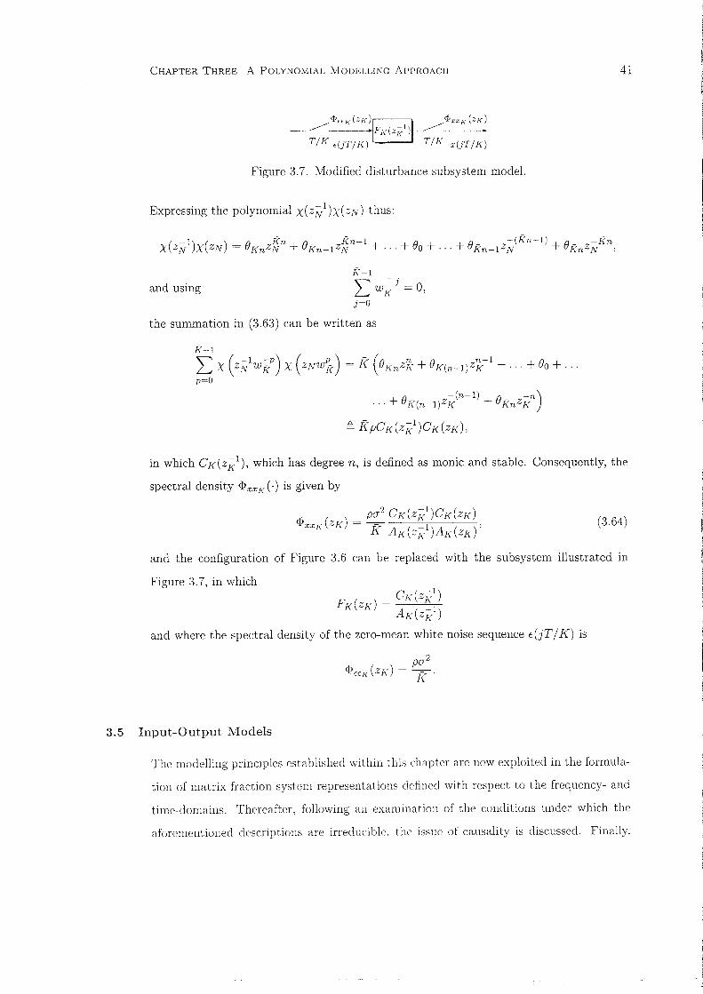
and using
CHAPTER THREE A POLYNOMIAL MODELLING ApPROACH
Figure 3.7. Modified disturbance subsystem model.
Expressing the polynomial X(Zj\/ )X(ZN) thus:
( -1) ( ) 8 Kn 8 Kn-l 8 8 -(Kn-l) 8 -KnX zN X ZN = KnzN + Kn-l zN + ... + 0 + ... + Kn-l zN + KnzN '
K-l + .LWj/=O,j=O
the summation in (3.63) can be written as
K-l
LX (zr:/wf!) X (ZNwj~J = k (8kn ZK+ 8k(n_1)z'j{-1 + ... + 80 + ...p=O
8 -tn-I) 8 -n)... + k(n-I)ZK + KnZK
b. - I= KpCK(Zi<. )CK(ZK),
41
in which CK(Zi<.I) , which has degree n, is defined as monic and stable. Consequently, the
spectral density <T?xXK(') is given by
(3.64)
and the configuration of Figure 3.6 can be replaced with the subsystem illustrated in
Figure 3.7, in which
and where the spectral density of the zero-mean white noise sequence E(jT / K) is
3.5 Input-Output Models
The modelling principles established within this chapter are now exploited in the formula
tion of matrix fraction system representations defined with respect to the frequency- and
time-domains. Thereafter, following an examination of the conditions under which the
aforementioned descriptions are irreducible. t he issue of causality is discussed. Finally.
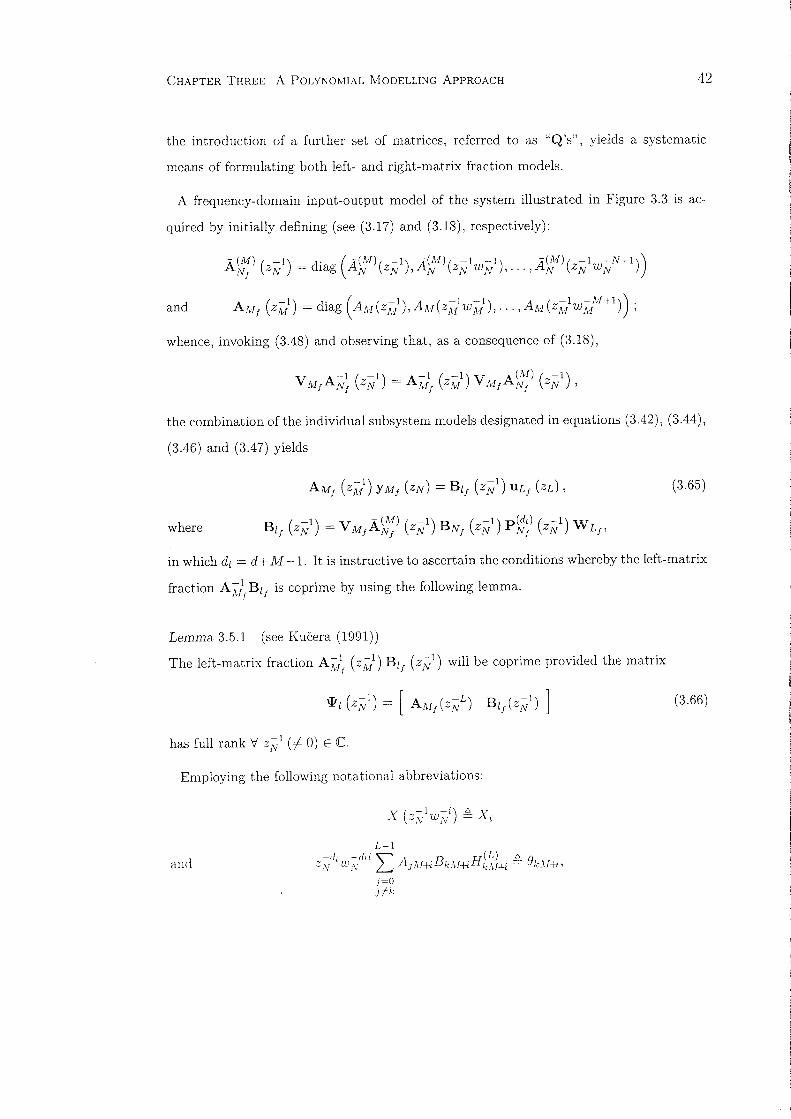
CHAPTER THREE A POLYNOMIAL I'vlODELLING ApPROACH 42
the introduction of a further set of matrices, referred to as "Q's", yields a systematic
means of formulating both left- and right-matrix fraction models.
A frequency-domain input-output model of the system illustrated in Figure 3.3 is ac
quired by initially defining (see (3.17) and (3.18), respectively):
A- (M) (,.-1) _ di (A-(AI) ( -I) A-(M)( -I -I) A-(M)( -I -N+I))Nf -N - lag N ZN ' N ZN W N , ... , N ZN W N
d A ( -I) di (A (-I) A (-I -I) A (-I -M+l))an M f ZM = lag AI ZM ' AI ZAI W M , ... , AI ZM W M ;
whence, invoking (3.48) and observing that, as a consequence of (3.18),
the combination of the individual subsystem models designated in equations (3.42), (3.44),
(3.46) and (3.47) yields
where
(3.65)
in which dl = d+ M -1. It is instructive to ascertain the conditions whereby the left-matrix
fraction A Alf Bl f is coprime by using the following lemma.
Lemma 3.5.1 (see Kucera (1991))
The left-matrix fraction AAf~ (zAn B1f (ZA/) will be coprime provided the matrix
has full rank I;j z-;/ (of: 0) E C.
Employing the following notational abbreviations:
Y ( -I -i) 6 V..: zj.v wl'vr == ""-\..i
(3.66)
and

CHAPTER THREE A POLYNOMIAL MODELLING ApPROACH
the matrix Wz is given by
i.-,
LAjM 0 0 ()o ()(Lr-l)M ()M
j=OL-l
0 LAjM+l 0 ()M+l ()1 ()2M+l
Wz= j=O
L-l
0 0 L AjM+M-l ()N-M+l ()N-2M-l ()N-l
j=O
43
At this juncture, the effect on WZ of setting Zi/ equal to f.L (E C) is ascertained, where f.L
is a zero of A (Zt'/) (i.e., A o). Since H(L) (zA;l) (i.e., H o) is present in the terms ()(L-l)M,
()(L-2)M, ... , ()M, in the first row, Wz can have full rank if and only if the minor
A1-1 L-l N-l
()o L L AjM-t-i = f.LdlB (f.L) H(L) (f.L) II A (f.LWi'/);=1 j=O ;=1
N-l
is not zero, whence f.L must not be a zero of H(L) (zi'/) or II A (Zt,/Wt/)·;=1
Observing that the zeros of H(L) (Zt'/) , namely,
correspond to s-plane zeros at
s = j (L+kN)ws,j (2L+kN)ws, ... ,j ((M -1) L+kN)ws, k = :1: 1, :1:2, ... ,
and that respective poles of G(s) at
s=J+jw and s=J+jw+j(IN-i)ws, 1=0,:+:1,:1:2, ... ,
constitute zeros of A (z:~/) and A (zA/w;/) at
then. in addition to the foregoing assumptions that A (zN1) and B (zNI) do not contain
a common factor, AM f and B Zf will be coprime if and only if the plant G(s) does not
contain poles:

CHAPTER THREE A POLYNOMIAL MODELLING ApPROACH
(1) at s=j(iL+kN)ws , i = 1,2, ... ,AI-1, k= :+:1, :+:2 ... ;
(2) at s = (J + jw and s = (J + j0, such that 0 - w = lws , l = :+: 1, :+:2, ....
44
Designating ALf and AV;) in an analogous fashion to AAlf and Ar:;), respectively (see
(3.65)), then, since it can be shown from (3.49) that A;V~WLf can be written as
again uniting equations (3.42), (3.44), (3.46) and (3.47), the relationship between YMf and
ilLf may be defined in right-matrix fraction form as
where
(3.67)
in which d; = d+L-l. The irreducibility ofthe matrix fraction BrfAr:; can be determined
from the following lemma.
Lemma 3.5.2 (see Kucera (1991))
The right-matrix fraction n,f (z;v1) A r:; (zL1) will be coprime provided the matrix
has full rank \:j z;Vl (:f 0) E C.
Using the notational abbreviations:

CHAPTER THREE A POLYNOMIAL MODELLING ApPROACH
the matrix IlJ r is arranged thus:
M-l
L A j L 0 0j=O
M-l
0 L A j Lrf-l 0j=O
M-I
IlJ r = 0 0 L Ajl+L-Ij=O
cPo cP(L-I)M cPM
cPM+l cPl cP2M+I
45
cPN-M-I cPN-2M-l cPN-I
Omitting detail of the relevant manipulations, then employing a similar argument to the
left-matrix fraction case, it can be shown that the conditions on the poles of G(s) such
that BrjAL; is coprime correspond exactly to those related to AM~BlJ"
The time-domain model corresponding to equation (3.65), obtained by combining the
subsystem models defined by equations (3.36), (3.37) and (3.38) and employing the fol
lowing relationship emanating from (3.32), namely,
V A - l ( -1) - A-1( -1)V A-(M)( -1)]\[Nq -Mq MNq,
where A}!;1)(q-l) is related to A(M)(qJ:/) in a similar manner to, A(q-l) and A(qN1)
respectively, (see (3.9b) and (3.37)), is given by
with
YM(O) = A~l(q-I)Bl(q-l)udO),
B/( q-l) = V,\I A}!;1) (q-l)B N (q-l )p~il(q-l)WL.
(3.68)
Correspondingly, observing that from (3.34),
A -. 1( -1)W - A-(L)( -1)W A- 1( -1)S q L- N q L L q .
then, again uniting equations (3.36), (3.37) and (3.38), the right-matrix fraction represen-
tation is
(3.69)

CHAPTER THREE A POLYNOMIAL MODELLING ApPROACH 46
where B ( -I) - V A-(L)( -I)B ( -I)p(dr ) ( -I)Wr q - AI N q N q N q L·
Of course, it is possible to acquire the models of equations (3.68) and (3.69) from the
corresponding frequency-domain descriptions of equations (3.65) and (3.67) by invoking
the following transformations (see (3.51)):
whence
The Bl(q-I) and Br(q-I) matrices can be expressed in terms of matrix-valued backward
shift operators, designated as "Q'S" , which fulfil an analogous role to the P's in the context
of square matrices and are specified as follows: if i = ul: + l, [E [0,L - 1],
Q (i ) ( -I) ~ -IlV p(Ml)( -I)W _ -IlQ p(l)( -I)ML q - q M N q L - q 0 L q (see (3.34)), (3.70)
where
Thus, for example, defining
then, supposing for simplicity of exposition that the parameter d is unity, B 1(q-l) In
equation (3.68) can be written as
(3.71a)
where Blj = diag (,6(j-I)M+M-l' P(j-I)Af, P(j-I)Af+I, ... , P(j-I)M+M-2) ,
AI-I
in which P(j-l)AI+i = L 7](j-I)Af+i-m·m=O
Correspondingly, in similar circumstances, if
then Br(q-I) in equation (3.69) may be expressed as
n+l
B ( - I ) 'B" Q(j) (-I)r q = L-t r) .\/ L q ,
)=1
(3.71b)

CHAPTER THREE A POLYNOMIAL l\lODELLING ApPROACH 47
udO)
Figure 3.8. Overall lifted system model.
in which n., is defined similarly to BI· and, with 17k replaced with Xk, each (3 term remainsJ J
as specified in equation (3.71a).
As a consequence of the considerations in the previous section regarding the disturbance
signal, it is supposed that a fast-rate model specified by the polynomials A (zf:./ ) and
C(zi:/) has been replaced by the following single-rate model (see (3.64)):
(3.72)
The disturbance subsystem thus can be described during the repetitive time interval by
the M moving average (!vIA) processes
which, using the modelling procedure dictated by equations (3.20), (3.21) and (3.22), may
be expressed succinctly via the relationship
YAJ (0) = A-;) (q-l)C AI (q-l )EIII (0)
= C ,H(«: )AA"l (q-l )EM (0). (3.73)
The overall lifted system model in right-matrix fraction format engendered by combining
equations (3.69) and (3.73) and illustrated in Figure :3.8 then is given by
(3.74)
There are two special cases of the multirate sampled-data system examined in this chap
ter which are worth further consideration, namely the instances whereby AllLor LIAI is

CHAPTER THREE A POLYNOMIAL MODELLING ApPROACH 48
an integer, as opposed to a rational number. The former situation is referred to in this the
sis as a fast output-sampled (FOS) system and the relevant open-loop time-domain model,
produced by replacing (L, M) with (1, N) in equation (3.74) and dependent equations is
YN(O) = AN1(q-l)b[(q-I)u(O) + ANI(q-I)CN(q-l)eN(O)
= br(q-l)a-I(q-I)u(O) + CN(q-I)AN1(q-l)eN(O), (3.75)
in which CN(q-l) denotes the matrix arising from the polynomial C(qN1) (see (3.24)),
where b B P (d+N- l ) b - A-(N)B p(d+N-l)1= N N WN, r - N N N WN
and (see (3.27))N-I
a(q-l) ~ L A (qNIW~).p=o
Accordingly, a fast input-sampled (FIS) system, defined as the case in which L = Nand
M = 1, is modelled thus:
in which
and
y(O) = a-1(q-l)b;(q-l)UN(O) + a-1(q-l)r(q-l)E(O)
= b~(q-l)ANl(q-l)UN(O) + ')'(q-l)a-I(q-l)E(O),
b- ' - 'A-(N)B p(d) b-' - 'B p(d)1- vN N N N' r - vN N N
N-l
,),(q-I) ~ L C (qN1w;;t).p=o
(3.76)
3.6 Illustrative Example
This section describes the formulation of polynomial matrix models that describe a multirate
sampled system conforming to the block diagram configurations of Figures 3.1, 3.2 and
3.:3. Following the establishment of individual subsystem models, both left- and right-
matrix fraction time-domain descriptions are acquired, in addition to a frequency-domain
interpretation. The procedure entailed in deriving an appropriate disturbance subsystem
model is demonstrated subsequently. This particular example is labelled 81.
Plant Description - Example 81
The plant to be considered has the transfer function
1G(s) = .
sisr - 1)(:3.77)
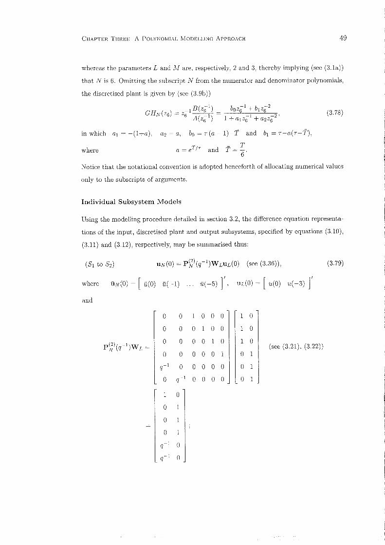
CHAPTER THREE A POLYNO~lIAL MODELLING ApPROACH 49
(3.78)
where
whereas the parameters Land M are, respectively, 2 and 3, thereby implying (see (3.1a))
that N is 6. Omitting the subscript N from the numerator and denominator polynomials,
the discretised plant is given by (see (3.9b))
B( -1) b -1 b -2GH (7) = 7-1~_ = OZ6 + l
Z6
N ··6/ -6 A(7.6-1) 1 -1 -'>,- +a1z6 + a2z6-
in which al = -(l+a), a2 = a, bo = T (a - 1)-1' and b1 = T-a(T-T),
a = eT IT and t: = !...6
Notice that the notational convention is adopted henceforth of allocating numerical values
only to the subscripts of arguments.
Individual Subsystem Models
Using the modelling procedure detailed in section 3.2, the difference equation representa
tions of the input, discretised plant and output subsystems, specified by equations (3.10),
(3.11) and (3.12), respectively, may be summarised thus:
(3.79)
where UN(O) = [ u(O) u( -1) ... u( -5) ]', udO) = [ u(O) u( -3) ]'
and
0 0 1 0 0 0 1 0
0 0 0 1 0 0 1 0
p~\q-l)WL =0 0 0 0 1 0 1 0
(see (3.21), (3.22))0 0 0 0 0 1 0 1
q-l 0 0 0 0 0 0 1
0 q-l 0 0 0 0 0 1
1 0
0 1
0 1
0 1
q-l 0
q-l 0

CHAPTER THREE A POLYNOMIAL MODELLING ApPROACH 50
(52 to 53) AN(q-I)YN(O) = p~\q-l)BN(q-l)UN(O) (see (3.37)), (3.80)
where YN(O) is defined similarly to UN(O),
AN(q-I) = 16 - (1 + a)p~I)(q-I) + ap~2\q-I)
1 -(1 + a) a 0 0 0
0 1 -(1 + a) a 0 0
0 0 1 (1 + a) a 0(see (3.24))
0 0 0 1 -(1 + a) a
aq-l 0 0 0 1 -(1 + a)
-(1 + a)q-I aq-I 0 0 0 1
and
where
and
YM(O) = V MYN(O),
YM(O) = [y(O) y( -2) y( -4) ]'
VM=[~~~~~~1'o 0 0 0 1 0
(3.81)
Time-Domain Descriptions
The individual subsystem models of equations (:3.79), (3.80) and (3.81) have limited prac-
tical application and, from both the perspectives of analysis and design, the respective left
and right- matrix fraction representations of equations (3.68) and (3.69) assume greater
significance. In the former instance, by defining the polynomial (see (3.18))
I
AM(q3 I) = IT A(q6Iw~3p)p=o
= (1 - (1 + a)q6 1 + aCf62) (1 + (1 + a)Cf61 + aq6
2)
2 -I 2-2= 1 - (1 + a )q3 + a Cf3 .
the denominator matrix AM(q-l) is given by (see (3.24))
(:3.82)

CHAPTER THREE A POLYNOMIAL MODELLING ApPROACH
Now, noting that (see (3.70))
and defining (see (3.17) for A(M)(-))
1 3
A- (Ml ( -1)B( -1) - II A( -1 -3P)B( -1) _ '" -iq6 q6 - q6 W6 q6 - ~ 7]iq6 ,
p=1 i=O
where 7]0 = bo, 7]1 = (1+a)bo+b1, 7]2 = abo+(1+a)b1 and 7]3 = ab1,
51
(3.83)
the numerator matrix Bl(q-l) in equation (3.68) may be specified thus (see (3.71a)):
in which
Bl(q-l) = diag (,62, ,60, ,6I) QOp~l\q-l)
+diag (,65, ,63, ,64) QOp~2)(q-l)
- r,65q~: ,62 ]- ,63q ,60 ,
,61 q-l ,64q-l
,63 = 7]1 + 7]2 + 7]:3, ,64 = 7]2 + 7]3 and ,65 = 7]3·
(3.84)
The denominator matrix Ar(q-l) in the corresponding right-matrix fraction is dictated
by Ar(q:L1) , namely (see (3.18)),
2
A ( - 1 ) IIA( -1 -2p ) 1 (1 3) -1 3-2L q2 = q6 WG = - + a q2 + a q2 ,
p=O
whence (see 0.24))
-1 :3 (1) -1 :3 (2) -1Adq ) = 12 ~ (1 + a )P2 (q ) + a P 2 (q ). (3.85)

CHAPTER THREE A POLYNOMIAL MODELLING ApPROACH
Specifying the polynomial
2 5
A- (L ) ( -1)B( -I) - IT A( -I -2P)B ( -1) _ , -iq6 q6 - q6 W 6 q6 - L Xiq6 ,p=l i=O
52
the numerator matrix Br(q-l) can be defined thus (see (3.71b)):
B r (q- l ) = diag(xo + Xl + X2, Xo, XO + xd QOp~I)(q-l)
+diag (X3 + X4 + X5, Xl + X2 + X3, X2 + X3 + X4) QOp~2\q-l)
+diag (0, X4 + X5, X5) QOp~3)(q-l). (3.86)
Frequency-Domain Representation
Observing that the frequency-domain model of equation (3.65) also can be obtained by
applying the transformation defined in equation (3.51) to the time-domain representation
of equation (3.68), the denominator matrix is given by
AM! (z31) = TAI(Z3)A M(z-1 )T:;:;J (Z3)
= diag (A\1(Z3 l) , AM(z3lw3l), ... , AM(Z3lw32)) , (3.87)
where AM(z3 1) is defined in equation (3.82). Designating the polynomial (see ((3.84))
5
B ( - 1) '{3 -i-l1 Z6 = L iZ6 '
i=O
the numerator matrix may be written thus:
(3.88)

CHAPTER THREE A POLYNOMIAL MODELLING ApPROACH
Disturbance Subsystem Model
53
The disturbance subsystem model initially requires the definition of BC), namely (see
(3.63)):
4
(1 + (1 + ) -I -2) (1 - -I - -2) '" B -i= a Z6 + aZ6 + CIz6 + C2z6 = 6 iZ6 ,
i=O
where
The polynomial
(3.89)
then is designated as the stable solution of (see (3.63))
to 0(z,lw2')0(zov,) ~ 2 (0004 21+ (to Oi Oi+2) Z3 + to 01
+ (to OiOi+2) z31 + 0004Z32)
= 2pC lvI ( Z:; I ) C M ( Z3 ) .
The numerator matrix C M (q-l) in the representation of equation (3.73) is arranged as
AM(q-l) (see (3.83)), with -(1 + a) and a replaced by CM l and CM2' respectively.
3.7 Conclusion
The work contained within this chapter represents the theoretical core of this thesis. The
key contribution to multirate-sampled system theory concerns the embedding of the prin-
ciples underpinning the decomposition procedures within a modern control framework. In
the latter respect, it will be noticed that the algebraic properties related to the polyno-
rnial matrices involved facilitate the computer-aided analysis of multirate configurations.
Furthermore, in contrast with single-rate system theory, the representations established
in this Chapter are characterised by having alternative interpretations in the time- and
frequency-domains.
CHAPTER FOUR
A GENERAL SYSTEM MODEL
This chapter describes how the polynomial modelling techniques developed in Chapter 3
can be applied to multivariable multirate-sampled systems. Thus, whereas the lifted single
input single-output (SISO) plant and disturbance subsystem models emanate from pulse
transfer functions defined with respect to the short time interval, the corresponding multi
input multi-output (!VIIMO) representations are predicated upon fast-rate m.itrix fraction
descriptions. As a consequence, it is neither practicable nor particularly beneficial to define
the elements within lifted polynomial matrices in the comprehensive detail prescribed in
the scalar case.
Using the artifice of fast-rate sampling switch insertion discussed in Chapter 3, section 4.1
views a multivariable system, in which each of the inputs and outputs are sampled at
dissimilar intervals, as comprising distinct input, discretised plant and output subsystems.
An overall lifted representation is acquired by initially combining a fast-rate lifted model
of the discretised plant with a block diagonal matrix that encapsulates the dynamics of
the zero-order holds. Thereafter, the required model in left-matrix fraction form results
by eliminating from consideration those output signals that are not required. Adopting a
corresponding approach, section 4.2 details the derivation of a compatible description of the
disturbance subsystem. The issue of causality is concentrated upon in section 4.3, in which
the arrangement of signals within system vectors in accordance with their related sampling
instants during the repetitive time interval leads to the characterisation of lifted system
matrices as being members of a particular "family". These so-called "repetitive time
interval index-dependent" representations are exploited subsequently in the dynamics
assignment and predictive control methodologies described in Chapter 5. The specification
of an accordant controller model in section 4.4 warrants an analysis of the absolute stability
and stability robustness of the closed-loop system, an exercise that is repeated for the SISO
systems examined originally in Chapter :3. The methods established in this chapter are
illustrated with the aid of a detailed example in section 4.5.
54

CHAPTER FOUR A GENERAL SYSTEM l'vIODEL
~TIL]
~TI L 2
55
ydt)
TIM]
Y2(t)
G(s)TI!>h
y",(t) »>
TI!>fm
Figure 4.1. The multirate-sampled multivariable plant.
4.1 The Multivariable Plant Model
The rnultirate-sampled l-inputjm-output plant to be considered is illustrated in Figure 4.1;
the respective sampling intervals of the control and output variables are T j L j s, Lj E Z,
j = 1,2 ... , l, and TfM, s, M, E Z, i = 1,2, ... , m, and exogenous disturbance signals
have been omitted for the present. Furthermore, it is assumed that
and
(4.1a)
(4.1b)
The time-scales referred to as the short time interval and repetitive time interval (see
(2.1a,b)) then are specified as
and
(4.2a)
(4.2b)
while it is also useful at this juncture to designate the parameters t., and NIi thus:
(4.3a)
and l'\;Ii = Njl\1i · (4.3b)
Recalling the modelling approach employed in Chapter 3 (see Figures 3.1, 3.2 and 3.3),
the relationship between the pulse-transforms of signals at the i th output and the lh
input can be expressed in terms of pulse-transfer functions designated with respect to the
short time interval ~ and, consequently, described via equations corresponding to (3.3),
(3.4) and (:3.5)- by inserting fictitious fast-rate samplers at the plant input and output.
Correspondingly, the system depicted in Figure 4.1 can be interpreted as the discrete-time

CHAPTER FOUR A GENERAL SYSTEM MODEL 56
Uds) inputU2(S) samplers U(ZN)
+Uds)
ZOHs
output
samplers
Yl(ZM,)
Y2(ZM2)
Figure 4.2. Discrete-time configuration.
configuration of Figure 4.2, in which Yd(ZN) symbolises the inclusion of m disturbance
signals and the subscripts M, related to the pulse-transforms of the outputs have been
omitted for concision. The mil matrix G pN(ZN) represents the fast-rate pulse-transfer
functions
ZN{Cij(S)H(N)(S)}, i=1,2, ... ,m, j=1,2, ... ,l,
whereas X(ZN) (E ek), indicating Y(ZN), Yd(ZN) (E em) or U(ZN) (E el), denotes
(4.4)
(4.5)
It is assumed that the matrix-valued pulse-transfer function GpN(ZN) can be expressed as
the following left-matrix fraction:
(4.6)
where (A, B) is coprime and in which it is further supposed that A(O) is upper-triangular
with
Aii(O) = 1, i = l,2, ... ,m.
Neglecting the disturbance signals for the time being, from comparison of equations (4.6)
and (3.9b) and by analogy with (3.11) and (3.37), the subsystem defined by GpN(ZN) can
be described by the time-domain model
A(q-I )5'(0) = p~~) (q-I )B(q-I )u(O)
= B(q-I )p;d) (q-I )u(O),
where:
(i) modifying the notation used in Chapter 3, with
xdO) = [.rdO) :rt,:( -1) ... xt,:( -N+ 1) r
(4.7)

CHAPTER FOUR A GENERAL SYSTEM MODEL 57
representing Yi(O) or Uj(O),
and
5'(0) = [ Y~ (0) Y; (0)
u(O) = [ u~ (0) u;(O)
Y~ (0) r (E ]RmN)
u;(O) r (E ]R1N);
(ii) the kNlkN matrix pf')(q-l) is designated as
(iii) if A(zt/) (B(zt/)) represents the (i, j)th element of A (zi:/ ) (B(zi:/)), then AN(q-l)
(BN(q-l)) constitutes the (i, j)th NIN block of the mNlmN matrix A(q-l) (mNllN
matrix B(q-l)).
The relationship between the lh fast- and slow-sampled controls is, from equations
(3.36) (with altered notation) and (4.3a), given by
in which
and
(Lj) () [_ - ] Iu j 0 = Uj(O) uj(-Lj) ... uj(-(Lj -l)Lj )
Hj(q-l) = p~j-l)(q-l)WLj
.
(4.8)
The l discretised zero-order holds H};j) (zN ), j = 1, 2, ... , l, then engender the following
time-domain model:
where
and
u(O) = H(q-l)U(O),
u(O) = [ uiLtl' (0) u~L2)1 (0) ... u;Ltl' (0) ] I
H(q-l) = block diag(H1(q-l), H 2(q-l), ... , H1(q-l)).
(4.9)
Combining equations (4.7) and (4.9), the fast-sampled outputs 5'(0) are related to the
slow-sampled controls U(O) thus:
where
(4.10)
The loss of information associated with sampling the output variables at integer multiples
of the short time interval is dealt with by separating each set of N fast-sampled outputs

CHAPTER FOUR A GENERAL SYSTEfvl MODEL 58
into those signals that are measured, namely, y;M;)( -kAlil, k E [O,2\;li - 1] (see (3.12)),
and the extraneous signals, namely, y;M;)(_L), L T klYli . Accordingly, introducing the
permutation matrix TIl, a vector Yr(O) comprising re-ordered output variables is defined
as
Yr (0) = TII Y(0), Yr (0) = [ y'(0) y~] I ,
[ ]
I ,where y(O) = y~lvIIl' (0) y~M2)1 (0) ... y~Im)1(0)
with y;M;) (0) specified analogously to u;Lj\O) (see (4.8)),
and I _ [ I I I ]',Y« - Yl e Y2e... Y m e
in which v.. = [ ... Yi(-L) . .. ]' LT kMi, k E [O,Mi 1] .
(4.11)
The plant model that results by applying the above transformation to equation (4.10) is
where
and
(4.12)
Designating the following matrix fraction, which is assumed to be coprime:
A -I( -I)A ( -I) = A. ( -I)A-I( -I)42 q 24 q 2 q 4 q ,
simple manipulation yields the lifted plant description
(4.13)
(4.14)
where
Notice that it is assumed that A h (q-l) specified above has a similar causal structure to
that of A1(q-I), which, for the present, can be defined as the requirement that the highest
possible powers of q in corresponding elements of these matrices are identical. The topics
of causality and matrix fraction conversion, including the term A.~21A 2 1 defined above,
will be examined in greater detail subsequently.

CHAPTER FOUR A GENERAL SVSTEt\! l\[ODEL 59
The alternative modelling approach described in section 3.3 can be extended to the
multivariable case by observing that, if the ",th element in any of the "time-domain vectors"
within equations (4.7), (4.9), (4.10), (4.11), (4.12) and (4.14) is
xd-jR), R = NIl{ (see (4.3a,b)),
then the ",thentry in the corresponding frequency-domain entity is
Consequently, the formulation of a frequency-domain representation of the multirate
sampled multivariable plant originates by using the following equation in place of equation
(4.7):
in which
Aj(Zi:/)Yj(ZN) = P~~(zl~/)Bj(z}./)Uj(ZN)
, -1' (d) -1 .c= Bj(ZN )Plj (zN )Uj(ZN),
where:
(i)
Y~(ZN) = [YiN(ZN) YiN(ZNWN) ... YiN(ZNW~-1)]',
with Uj(ZN) defined similarly;
(ii) the kNlkN matrix P~~\ZA/) is designated as
(4.15)
P' (A)(_-1) _ bl k di (p(A)(_-l) p(A)(~-1) p(A)( -1))kj .c.N - oc lag Nj "-N' Nj --N ' ... , Nj ZN (see (3.41));
(iii) if A( zA/) (B( z;\/)) represents the (i, j)th element of A(zt:;!) (B( Z"i:/)) , then ANj (zi:/)(BNj(zN1)) (see (3.42)) constitutes the (i,j)th NIN block of the mNlmN matrix
, -1 . ' -1Aj(z.v) (mNI1N matrix Bj(z;v )).
Similarly, using equations (3.44) and (:3.46), the input subsystem described in the time
domain via equation (4.9) can be modelled thus:
(4.16)

CHAPTER FOUR A GENERAL SYSTEM MODEL 60
where - (_ ) _ [ (Ltl' _ (L2)' (Lm)'] IUJ "-N - U l j (-oN) U2j (ZN) ... Umj (ZN) ,
in which, omitting the subscript j from each L j and Lj for clarity,
(L) [uJJ (ZN) = UJL (zr)
= [ UjL(Z~)
UJL (ZLWL)
UjL (z~w~)
and
where
HJ(ZN l) = block diag (Hlj(zN1
) , H 2j(ZNl
) ,
HJJ(zN l) = P>5j-
1\ ZN1 )W Lj (ZN).
Adopting an identical approach to that followed in the time-domain case, namely, com
bining equations (4.15) and (4.16), using the transformation
to obtain
and subsequently partitioning A T j and B T j as indicated in equation (4.12), the lifted
frequency-domain description is
(4.17)
It will be observed that, by invoking the time- to frequency-domain transformation spec
ified by equation (3.51), the vectors 5'J and uJ in equation (4.17) can be expressed as
(4.18a)
(4.18b)UJ(ZN) = Tii.(ZN)U(O) ,
Ty(ZN)=blockdiag(TM1(zf!1), TM2(Zf!2), ... , TfVfm(zf!m)) ,
with TiL (ZN) defined accordingly, whence the matrices AJ and BJ are related to A ane!
where
and
B in equation (4.17) as follows:
(4.19a)
and (4.19b)

CHAPTER FOUR A GENERAL SYSTEM MODEL
4.2 The Disturbance Subsystem Model
61
This section generalises the results obtained in section 3.4 to the multivariable case. In
common with the plant model derived above, the disturbance subsystem is specified ini
tially by a fast-rate pulse-transfer function matrix expressed in left-matrix fraction form.
Disregarding the plant at this stage, it is assumed that the disturbance subsystem is
described thus:
where
Y(ZN) = GdN(zN)e(zN),
GdN(ZN) = A-1(zj\/)C(zj\/),
(4.20)
in which C (z1:/) is stable, (A, C) is coprime and, again with a slight abuse of nota
tion, e(zN) signifies m zero-mean discrete-time white noise sources with spectral densities
O"f, O"~, ... ,0";'. By analogy with equations (4.6) and (4.7), the lifted representation asso
ciated with (4.20) is
(4.21)
with e(O) defined similarly to y(O) ((4.7)) and where C(q-l) is related to C(zj;/) in
an analogous fashion to A(q-l) and A(z}/). Invoking the transformation specified in
equation (4.11), the re-ordered description is
with
(4.22)
whence it is readily shown that
where (see (4.13)),
(4.23)
and in which ~(O) and 5'(0) ((4.11)) are arranged likewise.
In order to ensure compatibility with subsequent design methodologies it is necessary
to modify the above model by replacing the fast-sampled white noise sources with slower
sampled counterparts. In this respect, consider the relationship defined by the polynomial
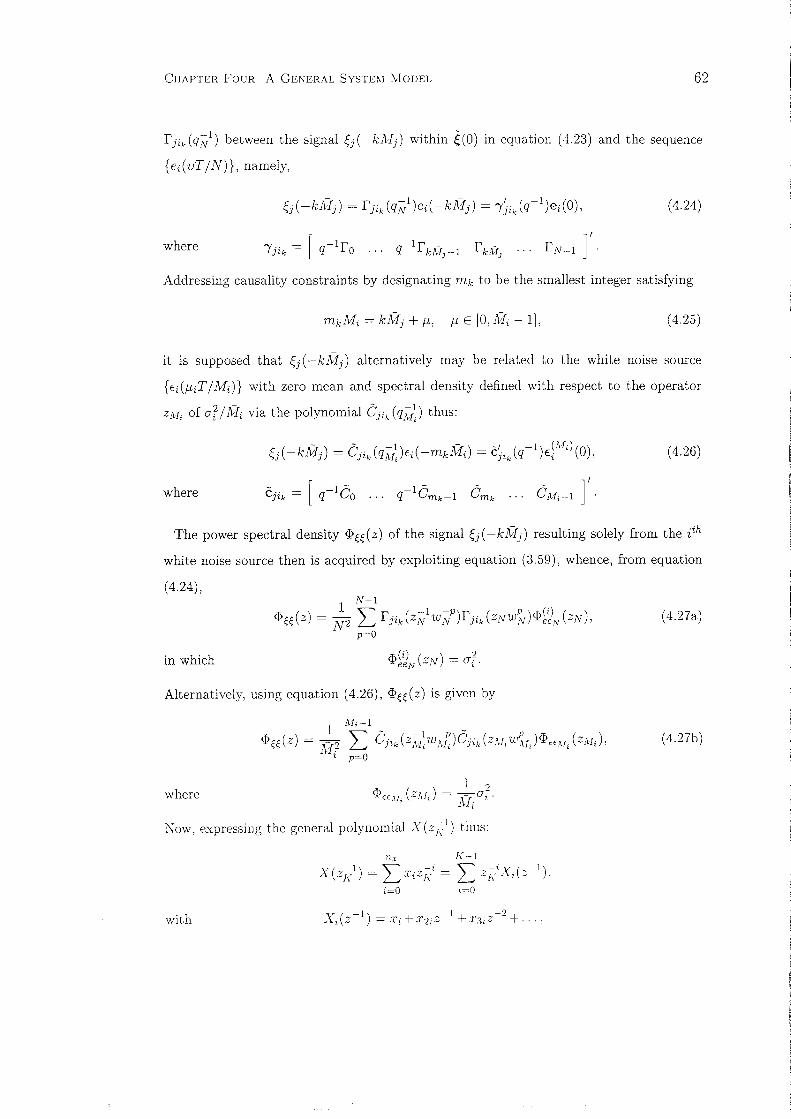
CHAPTER FOUR A GENERAL SYSTEM MODEL 62
fjik(qt:;!) between the signal ~j(-ki\Jj) within ~(O) in equation (4.23) and the sequence
{ei(vT/N)}, namely,
(4.24)
where
Addressing causality constraints by designating mk to be the smallest integer satisfying
(4.25)
it is supposed that ~j (-ki:lj ) alternatively may be related to the white noise source
{Ei (MiT/ Mi)} with zero mean and spectral density defined with respect to the operator
ZM, of aU i:fi via the polynomial Gj ik(q,\f~) thus:
where [ ],
c. - -1 - -1 - - -J2k - q Co ... q Cmk- 1 Cmk ... CMi-1
(4.26)
The power spectral density <p~~(z) of the signal ~j(-k1Vlj) resulting solely from the ith
white noise source then is acquired by exploiting equation (3.59), whence, from equation
(4.24),
in which
(4.27a)
Alternatively, using equation (4.26), <p~~(z) is given by
(4.27b)
1 ')where <P EE \ ! (ZM) = ~ai·
; t ' Ali
Now, expressing the general polynomial X (zA.t) thus:
Il x ]{-1
X( -1) , -i ,-i v ( -1)Z]{ = ~XiZ]{ = ~ Z1'; "\.; Z ,
i=O ;=0
with v (_-1) _ " +,,_-1 + >_-2 ,J\.;"" - .1; >12'L~ J :3,"" T· .. ,

CHAPTER FOUR A GENERAL SYSTEld l\IODEL
equations (4.27a,b) can be simplified by using
and consequently noting that
K-l K-l K-l
L X(zi/wi!)X(ZKW~) = L zi/wi/Xi(Z-l) L zkwkXi(z)p=O i=O i=O
K-l
= K L Xi(z-l)Xi(z).i=O
Thus, using equation (4.28), equation (4.27a) can be expressed as
63
(4.28)
(see (4.24)), (4.29a)
while, accordingly, equation (4.27a,b) becomes:
2 M;-l 2
1>i;i;(z) = ~i L C,,;(z-l)CK(z) = ~iCJik(Z-l)Cjik(Z) (see (4.26)).K=O
(4.29b)
Extending the principles governing equations (4.29a,b) to address the relationships be
tween the signals ~j(-kMj), k = O,l, ... ,1Yfj -1, j = l,2, ... ,m, and the discrete-time
white noise sources ti( -K,j'\:Ii ) , K, = 0,1, ... , M, - 1, i = 1,2, ... , m, the vector ~(O) in
equation (4.23) can be substituted by
~(O) = C(q-l )E(O),
where C(Z-l) constitutes the stable solution of
(4.30)
Therefore, from equations (4.23) and (4.30), the lifted disturbance subsystem model is
(4.31)
4.3 The Repetitive Time Interval Index-Dependent Model
This section describes an alternative lifted description in which the arrangement of signals
within vectors is dictated by their associated sample instants during the repetitive time

CHAPTER FOUR A GENERAL SYSTEM MODEL 64
interval. The resultant "repetitive time interval index-dependent" matrices present a
means of addressing causality issues and constitute a useful analytical tool.
Initially, using the symbol & in place of i (see (3.7)), the relevant sampling instants are
listed retrogressively as follows:
t. = O,/Ll, ... ,/Lo,··· ,/Le,
and
in which (see (4.1a,b)),
while it is supposed that permutation matrices 112 and 113 organise the entries within the
corresponding vectors accordingly. The vectors y(O) (and E(O)) and u(O) consequently are
defined as:
(4.32)
where Ym(O) ] / ,
with E(O) designated likewise, and
where
u(O) = 113u(0) = [u~(O) Ul( -Ad
uo(O) = [ Ul (0) U2(0)
Uj(-Aq,) ... Ul(-A1»]"
Ul(O) ]'
(4.33)
Applying the above transformations to the model obtained by uniting equations (4.14)
and (4.31) and disregarding the signals Ym(-/Ld and Ul(-Ad, the overall system descrip-
tion is
(4.34)

CHAPTER FOUR A GENERAL SYSTEM MODEL
with A(O) upper-triangular, in which
A OOll (0) = ... = A oomm(0) = ... = aoo(O) = ... = aee(O) = 1,
65
-lb' ( -1)q eo q
in which, with bO</J(q-1) denoting the element within B(q-1) relating Yi(-f-LO) to Uj(-A</J),
{
b 110 < A - dbe",(O) = O</Jo, r: - </J
0, f-LO > A</J - d.
With the provisos that the leading coefficients of its diagonal elements in general will not
be unity and that C(O) is block upper-triangular, C(q-l) otherwise is organised similarly
to A(q-l).
It is assumed that the open-loop system model of equation (4.34) can be expressed in
right-matrix fraction form as
(4.35)
in which (B a , A b) and (C a , A c ) are coprime. Given the arrangement of A, Band C above,
it is beneficial to confer a corresponding structure on each of the matrices in equation
(4.35), in addition to those defined subsequently, by specifying that if X(q-1) denotes the
denominator of a matrix fraction then X(O) is block upper-triangular. Consequently, while
their corresponding elements constitute polynomials with different degrees and coefficients,
it is possible to view certain matrices as being members of a set which have the same
dimensions and causally relate "repetitive time interval index-dependent" system vectors
identically. In this respect, the notation "Y rv X·' is introduced at this juncture to indicate
that "Y possesses a similar causal structure to X". Thus, for instance (sec (4.34)), A rv C.
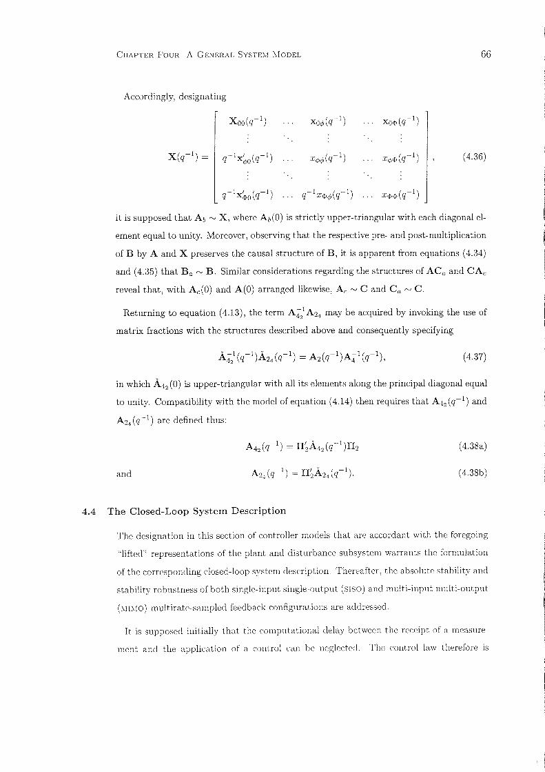
CHAPTER FOUR A GENERAL SYSTEM MODEL 66
Accordingly, designating
XOO(q-l) XO",(q-l) XO<1> (q-l)
X(q-l) = q-1X~O(q-l ) X<!)(t,(q-l) Xq,<1>(q-l ) (4.36)
q-1X~O(q-l ) -1 (-1) X<1> 1> (q-l )q .1:<1>q, q
it is supposed that A b '" X, where Ab(O) is strictly upper-triangular with each diagonal el
ement equal to unity. Moreover, observing that the respective pre- and post-multiplication
of B by A and X preserves the causal structure of B, it is apparent from equations (4.34)
and (4.35) that B a '" B. Similar considerations regarding the structures of ACa and CAe
reveal that, with Ae(O) and A(O) arranged likewise, A, '" C and C a '" C.
Returning to equation (4.13), the term A 421A 24 may be acquired by invoking the use of
matrix fractions with the structures described above and consequently specifying
A -1( -1)A (-1) - A ( -1)A-1( -1)42 q 24 q - 2 q 4 q , (4.37)
in which A42 (0) is upper-triangular with all its elements along the principal diagonal equal
to unity. Compatibility with the model of equation (4.14) then requires that A 42 (q-l) and
A 24 (q-l) are defined thus:
and
(4.38a)
(4.38b)
4.4 The Closed-Loop System Description
The designation in this section of controller models that are accordant with the foregoing
"lifted" representations of the plant and disturbance subsystem warrants the formulation
of the corresponding closed-loop system description. Thereafter, the absolute stability and
stability robustness of both single-input single-output (SISO) and multi-input multi-output
("II"ro) multirate-sampled feedback configurations are addressed.
It is supposed initially that the computational delay between the receipt of a measure
ment and the application of a control can be neglected. The control law therefore is

CHAPTER FOUR A GENERAL SYSTEM MODEL
realised by an algorithm which is specified thus:
67
(4.39a)
where R rv X and, with 8¢>()(q-l) defined as the polynomial relating Uj(-A¢» to Yi(-f.1()),
where the structure imposed on the "numerator" matrix by causality constraints is
in which{
8¢>()o' A¢>:S f.1()8¢>8(0) =
0, A¢> > f.1().
An alternative model, in right-matrix fraction form, is
(4.39b)
in which R s rv C and S; rv S. Notice that, if necessary, it is relatively straightforward
to accommodate computational lags within the numerator terms Sand S, above, while,
if the compensator constituted a dynamical system specified by a matrix-valued transfer
function, the pairs (R, S) and (Sr, R s ) would be obtained via the procedure followed to
engender (A,B) ((4.34)) or (B a , A/» ((4.35)).
Prior to defining the corresponding SISO models, it is useful to address causality issues by
designating the parameter mi. Thus, the control u( -lM), l E [0, L-1], is dependent upon
the measurements y(-mIL), y(-(ml + l)L), ... , in which, using the Euclidean division
property, m; (E [0, M]) is obtained from
(4.40)
where, if M > L, then each of the indices rn; will be distinct. On the other hand, if
L > j\I, there will exist at least two identical indices mj and mj+ 1, implying that the
most recent output signal employed by both the controls u( - j AI) and u( - (j + 1)M) will
be y( -miL). Notice that, ifmj = AI, then the most recent output signal used by u( -j1\I)
will be y(-N).
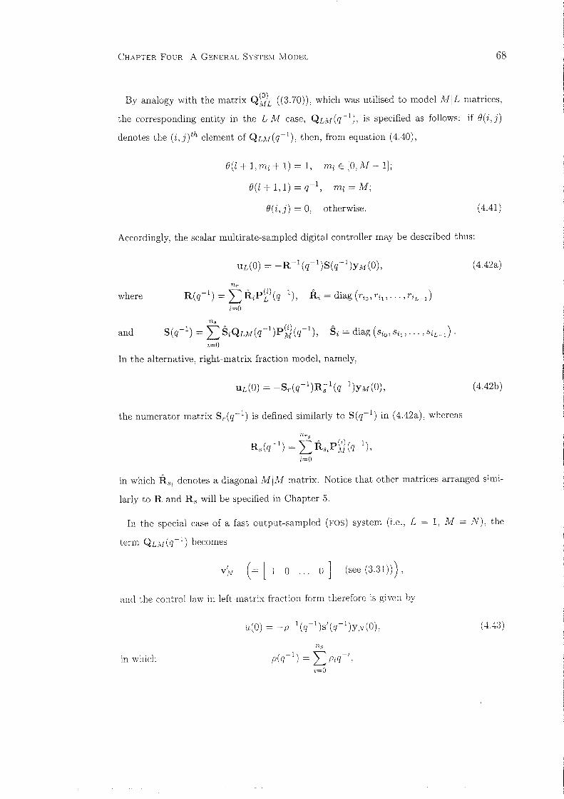
CHAPTER FOUR A GENERAL SYSTEM J\IODEL 68
By analogy with the matrix Q~~L ((3.70)), which was utilised to model MIL matrices,
the corresponding entity in the £1 M case, QUI (q-l ), is specified as follows: if B(i, j)
denotes the (i,j)th element of QU,J(q-l), then, from equation (4.40),
BU + 1,ml + 1) = 1, m; E [0, M - 1];
B(l+ 1,1) = «', m; = M;
B(i,j) = 0, otherwise.
Accordingly, the scalar multirate-sampled digital controller may be described thus:
(4.41)
wherenr
R(q-l) = L RiP~\q-1), Ri = diag ha' Til"'" TiL_I)i=O
(4.42a)
ns
and S(q-l) = LSiQLM(q-1)P~(q-l), s, = diag (Sio,Sil"" ,SiL_l)'i=O
In the alternative, right-matrix fraction model, namely,
the numerator matrix Sr(q-1) is defined similarly to S(q-1) in (4.42a), whereas
n r s
R ( - 1) "" R p(i) ( -1)S q = L.... s, M q ,
i=O
(4.42b)
in which RS i
denotes a diagonal MINI matrix. Notice that other matrices arranged simi
larly to Rand R, will be specified in Chapter 5.
In the special case of a fast output-sampled (FOS) system (i.e., L = 1, M = N), the
term QLM(q-l) becomes
v'» (= [1 0 ... 0] (see (3.31))) ,
and the control law in left-matrix fraction form therefore is given by
in which
np
p(q-l) = LPiq-i,
i=O
(4.43)

CHAPTER FOUR A GENERAL SYSTEM MODEL 69
flO) u(O) y(O)
Figure 4.3. Closed-loop multirate-sampled MIMO system.
and
ns
S/(q-1) = L SiV~PW(q-1)i=O
= [ So + sNq-1 + ... Sl + SN+1q-1 + ... ... SN-1 + s2N_1q-1 + ... ] .
In the complementary scenario (i.e., L = N, M = 1), referred to in Chapter 3 as a fast
input-sampled (FIS) system, the QLM (q-1) matrix becomes
P (N- 1)( -1)N q WN ( = [1 «: ]/
-1... q (see (3.21) and (3.33))) ,
whence the corresponding controller is
where, with L replaced by N, R(q-1) is as defined in (4.42a), and
n s
( -1) _ '""' S' .p(N-1)( -1)S q - 0 'N q WN
i=O
(4.44)
A block diagram model of the multirate-sampled MIMO feedback system is depicted in
Figure 4.3, in which, omitting the arguments for concision and generality,
and
(see (4.:34) and (4.35))
(see (4.42a,b)),
and where Yd and f denote "lifted" disturbance and reference signals with similar dimen
sions to, respectively, Y and u. The signals y and 11 are related to Yd and f via the
sensitivity functions 51 and 8 2 as follows:
(4.45a)

CHAPTER FOUR A GENERAL SYSTEM i'vIODEL 70
and (4.45b)
Now, observing that 8 1 and 8 2 may be defined in terms of polynomial matrices thus:
and
the closed-loop "denominator" matrix is given by, alternatively,
and
(4.46a)
(4.46b)
Defining the closed-loop characteristic polynomial (CLCP) thus:
(4.47)
the closed-loop system will be asymptotically stable if and only if OOcl(z-l) is stable.
Substituting (A,B) and (Ba,Ab) in (4.46a,b) with (AM,BI) ((3.68)) and (Br,AL)
((3.69)) and with (Sr,Rs) and (R,S) as specified in equation (4.42a,b), the above result
applies equally to the SISO multirate-sampled feedback system. In the scalar FOS scenario,
the CLCP is given by (see (3.75) and (4.43))
(4.48)
whereas (see (4.44)), defining Ps(z-l) = det (R(z-I))
and
the CLCP in the corresponding FIS configuration, obtained from equations (3.76) and (4.44),
IS
(4.49 )
(see (4.43)),
In both the FOS and FIS cases it is possible to gauge relative stability by determining
the return ratio Q( z), namely, the pulse-transfer function of the system elements enclosed
by the sampler operating at T s. Thus, observing that the FOS control law corresponds to
the following "implicit" pulse-transfer function (cf. (2.16) and (2.17))
. S(z:;:;!)I\y(zy) = p(z~l)

CHAPTER FOUR A GENERAL SYSTEIvI MODEL
the return ratio in this scenario is given by
Q(Z) = Z {f{N(ZN )GHW)(ZN)H~)(ZN)} (see (3.4) and (3.5))
S/(Z-I )br(z-I)p(Z-l)O:(Z-l) .
71
(4.50)
The gain and phase margins can then be ascertained in the usual manner by plotting the
frequency response
Q(ej wT) , wE [O,7f/T).
Evidently, a similar approach may be used to evaluate the stability margins in the FIS
system.
The assessment of relative stability via conventional frequency responses in general
multirate-sampled S1S0 feedback systems is not possible since the return ratio cannot
be expressed as a pulse-transfer function. However, invoking results customarily associ
ated with continuous-time multivariable control theory, Thompson (1986) has described
how in this instance the gain and phase margins may be defined as the least conservative
of those engendered by the characteristic gain loci of an open-loop model obtained via
the switch decomposition technique. This approach corresponds to plotting "ULj (e j wT ) ,
i = 1,2, ... ,L, or "UMj(ej wT) , j = 1,2, ... ,lVI, where the "ULj(Z)'S denote the eigenvalues
of
(4.51a)
and the "UMj (z)'s constitute the eigenvalues of
(4.51b)
Although the use of either QM (z) or QL (z) will yield the same result, it is more appropriate
from a practical perspective to employ QL (QJI[) when AI > L (L > M).
The problem of gauging the stability robustness of multirate-sampled multivariable sys
tems remains largely unresolved. However, in light of Thompson's technique, one possible
approach could involve determining
I:
'-1') '1'·z- ,-'····0 \J'
j=]
(4.52)

CHAPTER FOUR A GENERAL SYSTEM MODEL 72
where (Ji( z) denotes an eigenvalue of either 51 (z) or 52 (z) (see equations (4.45a,b)), with
K = M(L) and k = m(l)
4.5 Illustrative Example
The procedure entailed in establishing lifted representations of two multirate-sampled mul
tivariable configurations is demonstrated in this section. The first example, denoted M1,
is an unstable single-input two-output system, whereas the second concerns a two-input
two-output system labelled M2. In common with the scalar system examined in Chap-
ter 3, the parameter N is restricted to a low value in each instance to ensure expositional
clarity.
Example Ml
In this example, the vector-valued plant is described by
g(s) = l+1's - 1
(4.53)
and it is supposed that the signals Y1 (t), Y2 (t) and u( t) are sampled at intervals of, respec
tively, T / M 1 , T /u, and T / L 1 s, where
AlI = 1, !'vh = 3 and L 1 = 2.
Verifying from equation (4.2a) that N is 6, the pulse-transfer function model of the dis
cretised plant is
(4.54a)
where
in which at = a = e~T/6 and a2 = l/a £ a.

CHAPTER FOUR A GENERAL SYSTEM MODEL 73
Evidently, equation (4.54a) can be written as the following left-matrix fraction (see (4.6)):
where [:: ](4.54b)
Applying the techniques described in section 4.1, the fast-sampled outputs y(O) are
related to the slow-sampled control U(O) thus (see (4.10)):
A(q-l)y(O) = BH(q-l)U(O),
in which y(O) = [Yl(O) Yl(-l) ... Yl(-5) Y2(0) Y2(-1) ... Y2(-5)]',
u(O) = [u(O) u(-3) ] I ,
A(q-l) = block diag (16 - ap~l)(q-l),I6 _ ap~l)(q-l))
and, with B(q-l) =[blI6 ], pjd\q-l) (= p~l)(q-l)) =p~1)(q-l)
bI6
and (see (4.8) and (4.9))
(4.55)
owhere
o b2W3
q-1b2w3 0
The designation of the permutation matrix III in accordance with the following vectors
(see (4.11)):
Y(O) = [ Yl (0) Y2(0) Y2(-2) Y2( -4) ] I
and Ye = [Yl(-l) Y2(-1) yd-2) Yl(-:3) Y2(-3) Yl(-4) yd-5) Y2(-5)]',
leads to the plant model
(4.56)

CHAPTER FOUR A GENERAL SYSTEl\1 MODEL
A a(2,3) = A a(5, 4) = -a, A a(7, 1) = -aq-I, A a(8,2) = -aq-I;
74
and where
0 b1
0 b2
0 b1 0 b1
B1(q-l) =0 b2
B 2(q-l) =hq-l 0
with and0 b2 b2q-l 0
b -I 0 b.o:' 0L 2q lq
hq-l 0
b -1 02q
Using the left-matrix fraction A.421A 24 (see (4.13)), where
0') aa 0 a4 a5 0a a-
At2(q-l) = It A 24(q- l ) = -0 a 0 0 0 0 0 0
and0 0 0 0 a 0 0 0
0 0 0 0 0 0 0 a
the lifted plant description in left-matrix fraction form is given by (see (4.14))
(4.57)
1 - a6q-l 0 0 0
0 1 -'J 0-a-
0 0 1_'J-a-
0 -a2q-1 0 1
oab2q-l
(1 + ii)b2 q- 1 o

CHAPTER FOUR A GENERAL SYSTEM MODEL
Expressed as a right-matrix fraction, the plant model is (see (4.36)):
75
(4.58)
in which
and
(1 + a + a2 )a3b1q-l
-(1 + a + a2)ab2q-l
(1 + a - a4)ab2q-l
(1 + a)b2q-1 - ab2q-2
(1 + a + a2 )h
(1+ a+ ( 2 )b2
bz - (1 + a)ab2q-l
(1 - a4 - a5 )a2 b2 q- l
It will be observed that Ab(O) is upper-triangular and that the structures of Ba(O) above
and B(O) in equation (4.57) are identical. Notice that, since the elements within the
respective vector pairs 5'(0) and y(O), and U(O) and 11(0), are arranged identically, the
matrices A and :B in equation (4.57) equate to A and B in the repetitive time interval
index-dependent model ((4.34)).
It is supposed that the disturbance subsystem model is specified by the matrix
1+~2Z6']· (4.59)
Following the procedure summarised by equations (4.21) and (4.22), the vector ~(O) in
equation (4.23) is
in which
(4.60)
( -1) [ 5-111 q = 1 + a Clq a+ Cl
and oo
1
o
o 0
o 1 ~ 1·a+ C2

CHAPTER FOUR A GENERAL SYSTEM MODEL 76
The lifted disturbance subsystem model then is given by equation (4.31), with C(q-I)
designated as- - I 0 0 0CIa + Cllq-
C(q-I) =0 C20 C21 0
0 a C20 C21
0 - -I 0 C20c21q
where the parameters CIa, Cll' C20 and C21' which represent the stable solution of the spec
tral factorisation defined in equation (4.30), are determined from the following equations:
However, it is convenient to define C(q-I) alternatively as
l+clq-1 0 0 0
C(q-I) =0 1 C2 0
(4.61)0 0 1 C2
0 c2q-1 0 1
with_ Cll
and_ C21
CI = -_- C2 = -_-,CIa C20
and where the variances of the white noise sources {EI (-)} and {E2 (-)} have been scaled
accordingly. As mentioned above, the equivalence of the vectors y(O) and y(O), and
thus E(O) and E(O), implies that the matrix C(q-I) in equation (4.34) is identical to
C(q-I) above. Furthermore, it is relatively straightforward to establish that the matrices
Ac(q-I) and Ca(q-I) defining the lifted disturbance model in right-matrix fraction form
are identical to, A(q-I) and C(q-I) respectively.
Example M2
This example concerns the coupled-tanks system depicted in Figure 4.4, where
.4-7-- = /1, « 1).Al

CHAPTER FOUR A GENERAL SYSTEM MODEL
ut{t) U2(t)
t -II
T TYl Y2
1 1
Figure 4.4. Coupled-tanks system.
77
~
TIN
G(s)T
TIN
Figure 4.5. Sampling scheme for coupled-tanks system.
in which A 1 and A 2 denote the cross-sectional areas of tanks 1 and 2 and where the fluid
resistance Rf associated with the three valves are identical. The controls U1 (t) and U2(t)
represent the input flow rates in m 3/ s, while the outputs Y1 (t) and Y2(t) denote the water
levels in each tank. Linearised with respect to a specific operating point, the plant is
described thus:
with
y(s) = G(s)u(s),
1 [ s + 211G(s) = "-s2"-+-(2-+-2-11'--)s-+-3-11 ~L
(4.62)
In accordance with the desired rise times of the signals Y1(t) and Y2(t) in response to
respective step changes in reference inputs 1'1 (t) and 1'2 (t) in a closed-loop system to be
designed subsequently, the sampling scheme illustrated in Figure 4.5 is envisaged. From
equations (4.1a,b) and (4.2a.b), it can be established that
The matrix fraction representation of the cliscretisecl plant in equation (4.6) then may be
specified generically by
with d = 1.
Two particular scenarios shall be considered. namelv:

CHAPTER FOUR A GENERAL SYSTEM MODEL
(i) T = 0.15 S, N = J.L = 3, whence
al = 0.9012, a2 = 0.0552, as = 0.1232, a4 = 0.7438,
and b: = 0.0475, b: = 0.0039, bs = 0.0033 and b4 = 0.1297;
(ii) T = 0.15 s, N = J.L = 8, whence
al = 0.0214, a2 = 0.9617, as = 0.1271, a4 = 0.7420,
and b1 = 0.0184, b2 = 0.0015, bs = 0.0013 and b4 = 0.1297.
78
The step responses of both the continuous time and the sampled-data systems for scenario
(i) are presented in Figures 4.6 and 4.7, respectively. Notice that the model defined above
will be modified subsequently to produce a control law that incorporates integral action
in an illustration of multirate-sampled feedback system design in the next chapter.
4.6 Conclusion
This chapter has generalised the principles established for scalar systems in Chapter 3
to the multivariable case. Bearing in mind that the approaches utilised are conceptu
ally identical, the reliance of the lifted multi-input multi-output models on an original
non-unique matrix fraction description of the fast-rate discretised plant implies that they
cannot be specified in comparable detail to the corresponding single-input single-output
models. As reflected by the comments pertaining to the structures of the leading coeffi
cient matrices of each polynomial matrix, it will be observed that the notion of causality is
pivotal in defining the multirate-sampled plant and controller representations. In this re
spect, the so-called repetitive time interval index-dependent models, which naturally have
counterparts specified with respect to the frequency-domain, are exploited in the design
techniques formulated in the next chapter.

CHAPTER FOUR A GENERAL SYSTEM I'vloDEL 79
0.8
0.6
0.4
0.>"020.E 0.8
<C
0.6
0.4
0.2
0(l 1.5 4.j) 1,1
Time (s)
Figure 4.6. Step response of continuous time system.
0.8
0.6
0.4
0.20.>
"02
00-E 0.8
<C
0.6
0.4
0.2
0II 1.5 .l,jl 1.5
Time (s)
Figure 4.7. Step response of sampled data system.

CHAPTER FIVE
MULTIRATE-SAMPLED FEEDBACK SYSTEM DESIGN
The incorporation of the foregoing polynomial methods within the framework of estab
lished control design methodologies is addressed in this chapter. Specifically, dealing
principally with the multi-input multi-output (MIMO) case, it is demonstrated that the
lifted system models acquired previously are conducive to the synthesis of control laws via
the minimisation of quadratic performance criteria. Subsequently, means of enhancing the
flexibility of these design approaches are examined.
The chapter commences in section 5.1 with a summary of multirate LQG control design
by Kucera's polynomial equations approach. Following a proof of the main result, re
lated considerations, such as the determination of the "minimum degree solution" and a
dynamics-assignment interpretation of the optimal controller, are discussed. A numerical
example then is used in section 5.2 to illustrate the technique. In section 5.3 attention is
focused upon the modifications necessary to the Generalised Predictive Control strategy
to warrant its use in a multirate-sampling context, whilst a related numerical example in
section 5.4 demonstrates the use of the approach. Section 5.5 subsequently describes how
both the optimal and predictive control methodologies can introduce integral action within
the controller and incorporate dynamic weighting in the cost function. The feasibility of
solving the LQG "tracking" and "feedforward" problems is also discussed, following which
section 5.6 contains related numerical examples.
5.1 Optimal Control
The synthesis of feedback systems excited by stochastic disturbances via the minimisation
of a performancc index that penalises the output and control signal variances represents a
cornerstone of modern control. Known alternatively as optimal or Linear Quadratic Gaus
sian (LQG) control, the derivation technique customarily associated with the state-space
approach involves combining the solutions to t\VO separate problems, specified by Riccati
equations in each instance. This axiom, referred to as the ceriainiu equivalence princi-
80

CHAPTER FIVE l'vIULTIRATE-SAMPLED FEEDBACK SYSTEM DESIGN 81
ple or, simply, the separation theorem, implies that the optimal controller is engendered
by unifying the state estimator (namely, the celebrated Kalman filter), which provides
the best estimate of the system states from the observed outputs, and a linear feedback
control law (namely, the "Linear Quadratic Regulator" (LQR)), obtained by minimising
a quadratic performance index weighting the deviation from equilibrium of the output
and control signals in response to some initial perturbation. Optimal control has proven
to be effective in addressing some multivariable problems, although drawbacks pertaining
to a perceived lack of stability and performance robustness provided the motivation for
the development of synthesis methods, known generically as the Hoo approach, that use
information more commonly encountered in classical feedback system design via frequency
responses.
The polynomial equations approach to synthesising LQG controllers, attributed to Kucera
(1979) and Youla et al. (1976a,b), is the result of attempts to correct technical deficiencies
in contributions, such as Newton et al. (1957), made two decades earlier. Although its sig
nificance originally lay primarily in presenting a theoretical alternative to the state-space
approach, this methodology is now a practical proposition with the advent of POLYNOMIAL
TOOLBOX. Expositionally, the procedure adopted concerns an initial summary of the key
result as applied to the lifted representations derived in Chapter 4, followed by the proof.
Topics such as the non-uniqueness of the matrix fractions used and the interpretation of
the optimal control solution as a special case of dynamics-assignment are addressed sub
sequently. Additionally, certain enhancements to the method described are dealt with in
section 5.5. The computational issues associated with the proposed approach are detailed
in Appendix C, which additionally addresses a further design example.
The Multirate-Sampled LQG Control Law
Open-Loop System Model
It is assumed that the open-loop system is described thus:
((4.35))
where y(O) (and E(O)) and tl(O) are defined in, respectively, equations (4.32) and (4.33).
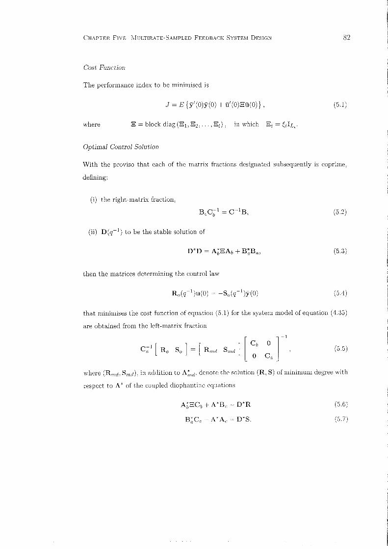
CHAPTER FIVE I'vIULTIRATE-SAMPLED FEEDBACK SYSTEM DESIGN
Cost Function
The performance index to be minimised is
J = E {:i (O)y(O) + U'(0)3u(0) } ,
82
(5.1)
where 3 = block diag (31,32 , ... ,31) , in which 3 i = ~JLi'
Optimal Control Solution
With the proviso that each of the matrix fractions designated subsequently is coprime,
defining:
(i) the right-matrix fraction,
B o.' - Co-lB'C b·- ,
(ii) D(q-l) to be the stable solution of
then the matrices determining the control law
(5.2)
(5.3)
(5.4)
that minimises the cost function of equation (5.1) for the system model of equation (4.35)
are obtained from the left-matrix fraction
(5.5)
where (Rmd, Smd), in addition to A~d' denote the solution (R, S) of minimum degree with
respect to A* of the coupled diophantine equations
(5.6)
(5.7)

CHAPTER FIVE l'vIULTIRATE-SAMPLED FEEDBACK SYSTEM DESIGN
Proof
83
The proof presented below is based upon the variational approach proposed by Sternad
and Ahlen (1993). The above result also may be established using the "completing-the
squares" method of Kucera (1979)
In seeking to establish the compensator which minimises the cost function of equation
(5.1), the effect of controller parameter variations on feedback system performance is
interpreted as being analogous to an appropriate feedforward contribution from the m
white noise sources represented by ("(0). Thus, the regulator is specified as
(5.8)
with K; and F defined as causal and rational, in which K, is assumed to be nominally
optimal and where the resultant closed-loop system is required to be stable.
Combining equations (5.8) and (4.35), both the output and control signals are separated
into the optimal entities Yo(O) and uo(O) and perturbations Yp(O) and up(O) resulting from
the variational term, namely:
where
(5.9)
in which
It will be observed from To and T I in equation (5.9) that, since the feedback loop is
unaffected, the control variation preserves stability. The performance index now may be
written as
where
and
.1 = .10 + 2.11 + Jz, (5.10)
The LQG control solution is obtained by determining K, such that, regardless of F,
.11 = 0 in equation (5.10). In this case no alternative controller could minimise .1 further,
since. from equation (5.10) . .10 and .h ('2: 0) are, respectively, entirely independent of,

CHAPTER FIVE J'vIULTIRATE-SAMPLED FEEDBACK SYSTEM DESIGN 84
(5.11)
and dictated solely by, the variational term. Accordingly, invoking Parseval's formula and
using tr (XY) = tr (YX), the cross term is given by
J1 = E { tr ((TOE)(Ba T 1FE)') - tr ( (gl/2KoTOE) (g1/2 Ab T 1FEY) }= 2
1. 1 tr (To:EF*T~B~_ g1/2KoTo:EF*T~Abg1/2) dz
7rJ Jlz l=l Z
1 i (* * (* *~K) )dz= -2. tr :EF T 1 B a - A b.::. 0 To -,7rJ Izl=1 z
in which E {E(O)E'(O)} = :E. Notice, that, since F and T 1 (and To) have been assumed
stable, the matrices F* and T~ in equation (5.11) contain poles in Izi > 1. Hence, to
obtain J1 = 0, it is required that
(5.12)
where, A* is a polynomial matrix whose invariant zeros lie strictly outside [z] = 1.
The diophantine equations (5.6) and (5.7) are obtained by:
(i) post-multiplying equation (5.12) by T 01;
(ii) expressing K; as the right-matrix fraction
where
(5.13)
(iii) using the right-matrix fraction defined in equation (5.2), whence equation (5.12) can
be written as
where
(5.14)
Introducing the coprime left-matrix fraction
it is evident that Q2 = XR and Q1 = XS,
(5.15)

CHAPTER FIVE l'vIULTIRATE-SAMPLED FEEDBACK SYSTEM DESIGN
or, equivalently, from equation (5.14),
B~Ca - A*A, = XS.
85
(5.16)
(5.17)
The problem then reduces to determining the matrix X. Post-multiplying equations
(5.16) and (5.17) by, respectively, C;I A, and C;;-I B a , adding the resultant equations,
utilising equation (5.3) and subsequently dividing by D*D, the ensuing identity is
(5.18)
It can be established now that
X=D*,
thereby implying that equations (5.16) and (5.17) are equivalent to equations (5.6) and
(5.7) respectively, since equation (5.18) then becomes the well-known Bezout identity
defining the coprimeness of the pair (B a , A b) , namely,
in which
MAb+NBa = I, (5.19)
Notice that M and N are stable, rational matrices free of unstable hidden modes, since
C,; C, and D are stable. Specifying (Rmd, Smd,A~d) to be the minimum-degree solution
of equations (5.6) and (5.7), the optimal controller is given by
or, alternatively, removing the factor related to the disturbance subsystem model by in
voking the left-matrix fraction defined in equation (5.5),
(5.20)
[J
Remarks
1. Non-uniqueness of l\Iatrix Fractions
The LQG compensator (Ro, So) remains unaffected if (B a . Ab), (Co, Ae) and (Be, C b )
are replaced by (BaU I , AbUd. (CaU:? AcU:?) and (B eU 3 , CbU3), respectively, where

CHAPTER FIVE MULTIRATE-SAMPLED FEEDBACK SYSTEM DESIGN 86
Ui(q,q-I), i = 1,2,3, denote unimodular matrices. The matrices used above to derive the
optimal control law therefore are neither unique nor require to be arranged as specified
in equations (4.35) or (4.36). Nonetheless, it is clearly advantageous from an expositional
perspective to deal with polynomial matrices in standard representative forms emanating
from the repetitive time interval index-dependent models designated in Chapter 4.
2. Minimum Degree Solution (Rmd, Smd, A~d)
In contrast with the single-rate case, the "solution (R, S) of minimum degree with respect
to A *" is not necessarily determined by a triple (R, S, A*) in which the highest power of q
in each column of A* is minimised and therefore requires clarification in this context. Since
it is shown subsequently that A is structured likewise to B, namely, using the notation
introduced in Chapter 4, A rv B, and that each row (column) of A (A*) consequently
represents sets of polynomials in qLj
I (qLJ, j = 1,2, ... , l, then A~d signifies the matrix
A* whose elements correspond to the solution with minimal degrees of qLj' j = 1,2, ... , l,
in each column. Expressing the k th column of A*, namely, XZ(q), thus:
,,* ( ) _ v k dk) + + ,,(k) nkAk q - AO + Al q . . . A n k q , (5.21 )
and defining the parameter 'Uk as denoting the total number of non-zero entities in A~k),
i = 0, 1, ... , nk, then A':nd is given by the solution in which each 'Uk is minimal.
3. Polynomial Matrix Structures
The structure of the matrix D specified by the spectral factorisation problem of equation
(5.3) may be ascertained by recalling that Ab rv X (see (4.36)) and B; rv B (see (4.35)).
Since X(O) is block upper-triangular and the zero entries with B(O) form a block lower
triangular sub-matrix, the (i,j)th elements of both AbSAb and B~Ba can be expressed
thus:
i < j
Z = J
i > i.
(5.22)

CHAPTER FIVE MULTIRATE-SAMPLED FEEDBACK SYSTEM DESIGN 87
Thus, since D*D and X*X possess similar structures, D rv X. Inspection of equation
(5.6), in which A;;BCb evidently is arranged similarly to X*X, then reveals that A rv B
and, additionally, confirms that R rv X (see (4.39a)). Furthermore, it is supposed that
Be rv Band C, rv X in equation (5.2), while Co rv X in equation (5.5).
4. Dynamics-Assignment Interpretation
The optimal controller can be derived instead via a single diophantine equation emanating
from equations (5.6) and (5.7). First, following the procedure adopted in deriving equa
tion (5.18), namely, post-multiplying equations (5.6) and (5.7) by Cb1A b and C~lB a ,
respectively, and summing the resultant equations, then removing the common factor D*
by invoking equation (5.3), it is established that
(5.23)
Now defining the right-matrix fraction
(5.24)
in which Al rv X, B I rv Band C I rv X, then post-multiplication of equation (5.23) by
C I engenders the polynomial matrix equation
(5.25)
which can be used as an alternative to equations (5.6) and (5.7). Moreover, it will be
observed that, when applied to equation (5.23), the matrix fraction defined in equation
(5.5) implies that the LQG controller (Ro,So) satisfies the diophantine equation
(5.26)
Equation (.5.26) reveals a fundamental property of optimal control, namely, that the
poles of the closed-loop system constitute the union of those resulting from the spectral
factorisation problem and those corresponding to the invariant zeros of the disturbance
subsystem numerator matrix, determined by the characteristic polynomials of D (q-l) and
Co(q-l) respectively.

CHAPTER FIVE MULTIRATE-SAMPLED FEEDBACK SYSTEM DESIGN
5. The 5I50 Case
88
In contrast with the terms BrA:L1 ((3.69)) and Clv/A::l ((3.73)) that define the respective
lifted plant and disturbance subsystem models in the general SISO case, the denominator
matrices within the remaining matrix fractions required in the optimal control solution and
its dynamics-assignment interpretation (see equations (5.2), (5.5) and (5.24)) in general
possess structures which do not conform to that of F K(q-I) in equation (3.24). Denoted by
X(q-l), it is assumed that Co, Co, C 1 and AI instead are organised thus (ef. (4.42a,b)):
n x
X(q-l) = LXiP~\q-I),i=O
(5.27)
with Xi = diag (Xio' XiI' ... , XiL_I) and where x, = h in the case of AI, whereas, denoted
by Y(q-l), whilst Be, A and B 1 can be specified as a summation of "Q" matrices, namely,
in which
ny
Y(q-l) = LYiQ~)L(q-l),j=1
(5.28)
the term Yim , unlike those designating Blj in equation (3.71a), cannot be associated with
a particular polynomiaL Notice that R o and So are arranged likewise to Rand S, respec
tively, in equation (4.42a).
The structure of the matrix D in the scalar scenario, defined as the stable solution of
the spectral factorisation problem ((5.3)), may be ascertained by introducing the following
results concerning the adjoints of the "Q" and "P" matrices:
(i)A ( (j-i))*v ; P L ,j > i
Yii , J = Z
p(i-j)y.. J' < iL 1)'
(5.29)
(ii) specifying i = I-LL + I, 1 E [0. L - 1],
IE[l,L-1]
1=0(5.30)

CHAPTER FIVE MULTIRATE-SAMPLED FEEDBACK SYSTEM DESIGN 89
Accordingly, from the definitions of AL (cf. Ff{(q-I) in (3.24)) and B, ((3.71b)), then,
using equations (5.29) and (5.30), in the general SISO case equation (5.3) becomes
( n )* ( n ) (n+ I ) * (n+ I )D*D = r, +~ aL;PY) h +~ aL;PY) + 6 ~BrjQ~)L ~ B rjQA1L
n n
=.6.0 + L.6.i (PY))* + LPY) .6.i ,
i=l i=l
where.6. i = diag (6io,6i1, ... ,6iL_l). Observing that, if i = f.LL + l, l E [O,L -1],
(5.31)
in which the rearranged diagonal matrix xW is given by
with xW = X, l = 0, then the matrix D may be expressed as
n n
D = L P~)Di = L D~~P~),i=O i=O
(5.32)
with Di = diag (dio,di1, ... .c.: and D~~ similarly defined, where the n, terms can be
acquired by solving the (n + I)L equations in (n + I)L variables specified by
n-j'\:"" '(J) , (J)s: DiD(t+j)R = f:!..JR'
i=O
j = 0, 1, ... , n. (5.33)
Consequently, D conforms to the structure of R in equation (4.42a).
A summary of the matrices and polynomials that define the optimal control solution for
the general SISO case and the scenarios hitherto referred to as fast output-sampled (FOS)
and fast input-sampled (FIS) is provided in Table 5.1.
5.2 Illustrative Example - Optimal Control
This section outlines the derivation of an LQC compensator for the system labelled Ml ,
which was examined originally in Chapter 4. Initially addressing the general solution,
attention focuses upon establishing the structures of each of the polynomial matrices
involved and, consequently, the nature of the difference equations that specify the optimal
control law. The dynamics-assignment approach then is utilised to acquire the LQC control
solution and related stability margins in a numerical example.

CHAPTER FIVE l'vIULTIRATE-SAMPLED FEEDBACK SYSTEM DESIGN
Table 5.l. Optimal control solution - 81SO case.
MIMO SISO FOS FIS
Ab A L 0: AN
Ba B,. b,. b',.
A e AM AN 0:
Ca CM CN I
Cb Cb I 'VI
Be Be CWlbl b'1
D D d D
A A A 5..'
R R p R
Ro Ro p R
8 8 5' S
80 80'C(Nl S5 N
Co Co I I
Al Al 0: AN
B1 B1dNlb b'N ,. r
C1 C1 I ~(
90
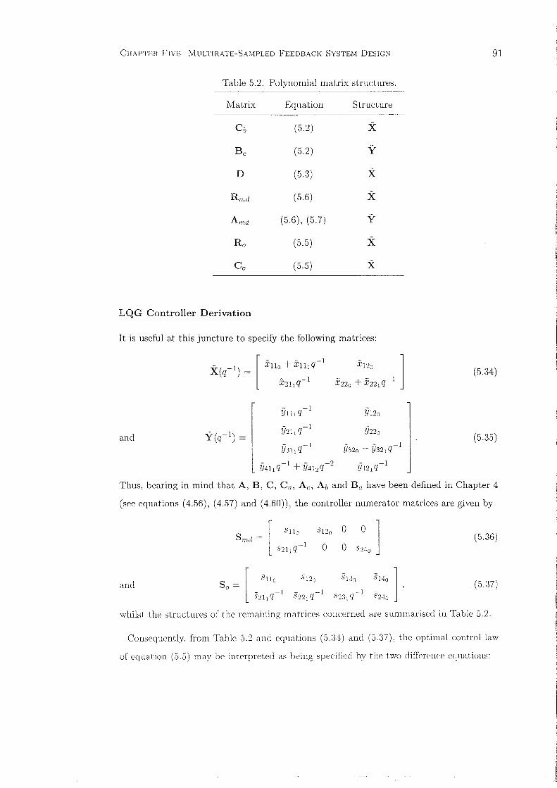
CHAPTER FIVE MULTIRATE-SAMPLED FEEDBACK SYSTEM DESIGN
Table 5.2. Polynomial matrix structures.
Matrix Equation Structure
C b (5.2) X
Be (5.2) y
D (5.3) X
Rmd (5.6) X
A m d (5.6), (5.7) Y
Ro (5.5) X
Co (5.5) X
LQG Controller Derivation
It is useful at this juncture to specify the following matrices:
91
- -1 [ xn,+ xn,«: X1 20 ] (5.34)X(q ) =- -1 - - 1X211q X220 + X221 q-
r
- -1Y120Y1hq
- -1Y 220
and Y(q-1) = Y211 q(5.35)
- -1 Y3 20 + Y 321q-1l Y3h q
Y411 «:' + Y 41zq-2- -1Y421q
Thus, bearing in mind that A, B, C, C a , A e , A, and B; have been defined in Chapter 4
(see equations (4.56), (4.57) and (4.60)), the controller numerator matrices are given by
[ snc 8120 0 0 ]Smd =-1 0 0 82·10821 1q
and So = ['1 Co .S120 .s 130 .SHa ],- -1 - -1 - -1
·hl o821 1q 8221q .52:01 q
(5.36)
(5.37)
whilst the structures of the remaining matrices concerned are summarised in Table 5.2.
Consequently, from Table 5.2 and equations (5.:34) and (5.37), the optimal control law
of equation (.5.5) may be interpreted as being specified by the two difference equations:

CHAPTER FIVE MULTIRATE-SAMPLED FEEDBACK SYSTEM DESIGN 92
TIlO11,(0) + T120 11,( -3) + TIll 11,(-6) = - (.SlloYI (0) + SI20Y2 (0)
+S13oY2( -2) + S140Y2(-4))
T22011,(-3) + T2\j11,(-6) + T22I11,(-9) = - (S211Yl(-6) + S240Y2(-4)
+.5220Y2(-6) + .5231Y2(-8))
(5.38a)
(5.38b)
Numerical Example
In this example it is supposed that:
(i) the repetitive time interval is
T = 6 loge 1.04 = 0.2353 s,
whence (see equation (4.54a)),
al = a = 0.9615, b1 = 0.0385, a2 = ii = 1.04 and b2 = 0.04;
(ii) the disturbance model is specified by (see equation (4.59))
Cl = -0.75 and C2 = -0.8;
(iii) the control weighting parameter is (see equation (5.1))
6 = 0.115.
Solving equation (5.3) for the above value of 6, it is found that
-0.6770
0.4648 + 0.2409,,-1 ] .
1 [ 0.4489 + 0.2492q-ID(q- ) =
-0.6865q-1
The closed-loop poles related to the plant - determined by the zeros of z2det (D(z-l))
then are given by
z = 0.3643 and z = 0.7899,
while those associated with the disturbance subsystem - dictated by the characteristic
polynomial of C o(z-1 ) (or, equivalently, C, Co, C, or C I ) are located at
z = 0.48:38 and z = (1.38:31.

CHAPTER FIVE MULTIRATE-SAMPLED FEEDBACK SYSTEM DESIGN 93
The dynamics-assignment approach to determining the LQG controller is dependent upon
the following matrices, obtained from the matrix fraction conversio.i defined in equation
(5.25):
-1.5452 ]
1 + 5.0951q-l '
-0.1050q-l
-0.0046q-l - 0.0215q-2
0.1157q-l - 0.0918q-2
0.0816q-l - 0.0802q-2
0.1110
0.1539 - 0.0822q-l
0.0400 - 0.0310q-l
0.0846q-l - 0.0473q-2
and-1 [ 1 - 0.4068q-l 0.0251 ]
C 1 (q ) =0.1790q-l 1 - 0.4556q-l
The minimal degree solution of the single diophantine equation ((5.25)), defined with
respect to R, is
[
0.4489 - 0.4485q-lRmd=
1.5529q-l
-0.0642 ]
0.4648 - 0.0154q-l
o0.6202 0 0 ]
o 0.6592[
-0.0308Smd=
0.0268q-land
The final stage of the derivation procedure concerns the right- to left-matrix fraction
conversion of equation (5.5). which yields
0.1634
0.4648 - O.0743q-l ][
0.4489 - 0.0931q-lRo =
0.2387q-l
[ -0.0308 0.6202 0.4505 0.3676 ]So =
0.0238q-l 0.5381q-l 0.3908q-l 0.6592
C,,~ [1 - 0.4304q-l 0.0613 ]and
0.0957q-l 1 - 0.4306q-l
Utilising the technique proposed by Thompson (1986), in which the return ratio is defined
as the path enclosed by the sampler at the controller output, the phase margin is

CHAPTER FIVE !vIULTIRATE-SAMPLED FEEDBACK SYSTEM DESIGN
whereas the upper and lower gain margins are given by
Glvlu = +16.4479dB and GM[ = -8.3904dB.
5.3 Predictive Control
94
The application of predictive control strategies was traditionally associated with self
tuning regulators, whereby an identification algorithm provides estimates of the system
parameters required to calculate the control law at each sample instant. Nevertheless, it
is important to emphasise that the ever-increasing sophistication of the predictive control
approach engendered by three decades of research implies that nowadays this methodology
is increasingly being viewed as an alternative to LQC controller design in the non-adaptive
context considered in this section. Additionally, in contrast with other control design
methods, predictive control affords the possibility of addressing system nonlinearities by
incorporating them as constraints when formulating the design problem. In this case,
the predictive control law is acquired by solving a constrained optimisation problem. The
specific approach described in this section concerns control algorithms customarily encoun
tered in an adaptive framework - referred to nowadays as model-based predictive control
(MBPC) - as opposed to the techniques known as "Model Predictive Heuristic Control"
(Richalet et al. (1978)) and "Dynamic Matrix Control" (Cutler and Ramaker (1979), Prett
and Gillette (1979)) commonly employed in the process and petrochemical industries.
Developments in MBPC emanate from Astrom and Wittenrnark's self-tuning regulator
(Astrom and Wittenmark (1973)), In this paper, a "minimum-variance" control algorithm
was introduced - namely, based upon information available at the k th sample instant, a
controller which minimised the variance of the output signal at the (k + d)th sample
instant, where d denotes the plant dead time. The inherent drawback in minimum
variance control in failing to guarantee the closed-loop stability of configurations con
taining nonminimum-phase plants provided the motivation for the Generalised Minimum
Variance (C:"IV) self-tuning controller (Clarke and Gawthrop (1975)), in which the control
and predicted output signals were weighted dynamically within the performance index.
Other notable contributions in :"lBPC are Peterka's predictive controller (Peterka (1984)),
Ydsr.ies extended-horizon design (Yelstie (1984)) and the EPSAC algorithm (De Keyser

CHAPTER FIVE MULTIRATE-SAMPLED FEEDBACK SYSTEM DESIGN
and Van Cauwenberghe (1982)).
95
The theoretical work contained in this section is founded upon the Generalised Predictive
Control (GPc) algorithm by Clarke et al. (1987a,b). While penalising the variances of
future controls, the GPC strategy attempts to drive the predicted outputs "close" to a
known reference signal throughout a "prediction horizon" from the (k1 + d)th to the (k2 +d)th sample instants, thereby resulting in a suggested sequence offuture controls. However,
only the control at the kfh sample instant is actually implemented and, in an adaptive
framework, the control law is re-calculated given new information available at the (k I + l)th
sample instant. Since the formulation of the problem is such that, if used, the set of future
controls would be applied in open-loop, this receding horizon approach belongs to the class
known as "Open-Loop-Feedback Optimal Control" (Bertsekas (1976)). This section details
the derivation of predictive controllers for the lifted plant model in left matrix fraction form
in Chapter 4, exploiting the underlying principles in extending the basic GPC technique
to the multirate-sampled case described by Truman and Govan (2000a). In common with
the procedure used to describe the LQG approach, modifications to the basic technique,
such as the introduction of integral action by adopting an incremental system model - the
customary formulation of the GPC design problem - are addressed in section 5.5. Notice
that, while the underlying principles remain unaffected, the derivation technique differs
somewhat from that employed by Clarke et al. (1987a,b).
Problem Outline
The forthcoming analysis deals with the "regulator" problem and concerns the derivation
with respect to a horizon p repetitive time intervals in advance of a predictive control law
at the sample instants denoted by t = Av , where (see section 4.3)
Initially, it is assumed that the output (and, therefore, the white noise) and control sam
pling instants are synchronised as follows:
(5.39a)
whereas it is supposed additionally that
(5.39b)

CHAPTER FIVE MULTIRATE-SAMPLED FEEDBACK SYSTEM DESIGN
output sampling instants
96
~N -J.l,.;+l
control sampling instants
-N -A" o (p-l)N pN-A u
Figure 5.1. Timing diagram.
where d denotes the dead time of the discretisied plant model (see (4.6)). As discussed in
the sequel, the proposed approach is not unduly restrictive and can be modified readily
to account for alternative situations.
Suppressing the subscripts i and j related to each control and output for concision,
the problem being considered may be summarised as that of obtaining the sequence
{u ov ( - Av ), ue; ( - Av - l ), ... , UOv (pN - Av +I)} minimising a quadratic performance in
dex that penalises the outputs y( -fLrJ, y( -fLK-r) , ... , y(pN - fLK+r), in addition to the
aforementioned controls. Thus, as depicted in the timing diagram of Figure 5.1, the pre
diction horizon is defined as t == pN - fLK+l- In common with the use of the GPC algorithm
in an adaptive context, the "optimal" predictive control at t == -Av then is specified to be
U Ov ( - Av ) , while the overall multirate-sampled predictive control law constitutes the amal
gamation of the individual controls u oo (0), U 0 1(-Ar), ... , UO'l> (-A¢). The primary focus
of attention therefore involves the formulation of an appropriate model -- the so-called "p
repetitive time intervals-ahead" representation - that encapsulates the problem defined
above.
p Repetitive Time Intervals-Ahead Representation
The predictive model is predicated upon the repetitive time interval index-dependent
description established in Chapter 4, namely,
((4.34))
Defining the following vectors,
(5.40a)
with "E(N - !L,,+l) specified accordingly, and
(5AOb)
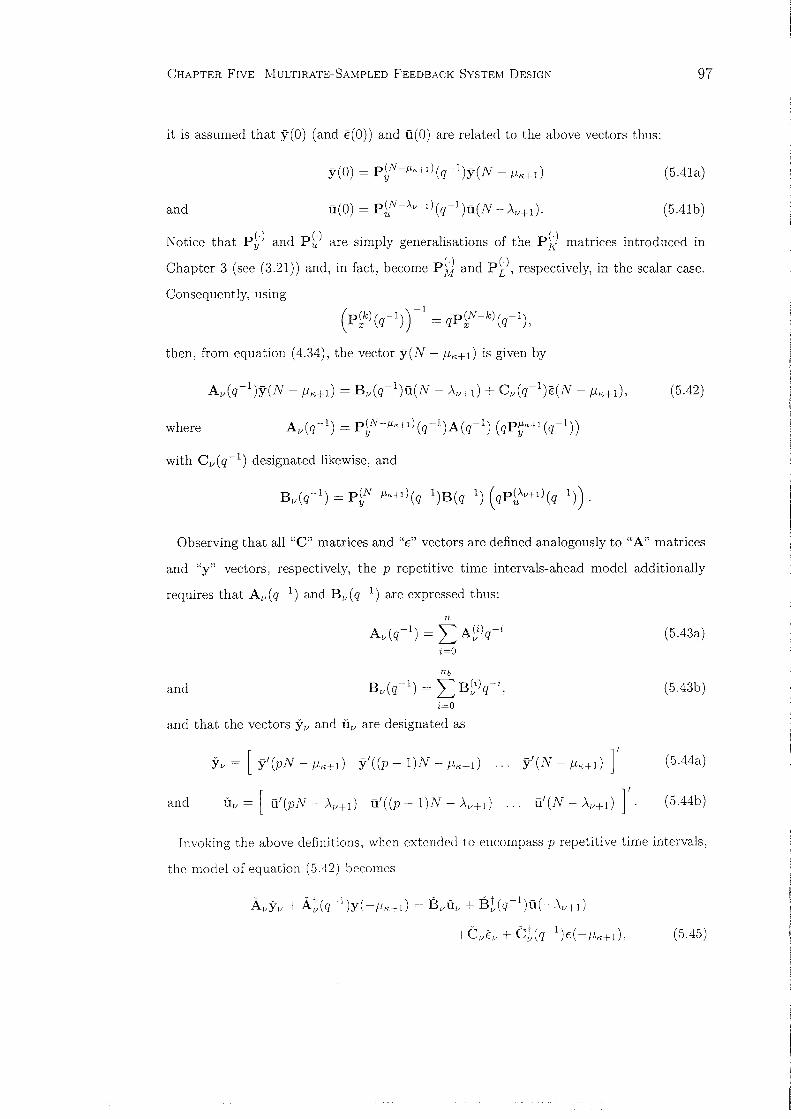
CHAPTER FIVE MULTIRATE-SAMPLED FEEDBACK SYSTEM DESIGN
it is assumed that y(O) (and E(O)) and ii(O) are related to the above vectors thus:
97
(5.41a)
and (5.41b)
Notice that p1') and pt) are simply generalisations of the P~ matrices introduced in
Chapter 3 (see (3.21)) and, in fact, become p~) and p~), respectively, in the scalar case.
Consequently, using
then, from equation (4.34), the vector y(N - f1K;+d is given by
where
(5.42)
with Cv(q-l) designated likewise, and
Observing that all "C" matrices and "E" vectors are defined analogously to "A" matrices
and "y" vectors, respectively, the p repetitive time intervals-ahead model additionally
requires that Av(q-l) and Bv(q-l) are expressed thus:
n
and
Av(q-l) = L ASi)q-i
i=O
nb
Bv(q-l) = L BSi)q-\i=O
(5.43a)
(5.43b)
and that the vectors yv and Uv are designated as
Yv = [ y'(pN -Ih+d y'((p - 1)N - f1K;+d y'(N - f1K;+1) ]'
and Uv = [ ii'(pN - Av+r) ii'((p - 1)N - Au+d ... ii'(N - Al/+r) ]'
(5.44a)
(5.44b)
Invoking the above definitions, when extended to encompass p repetitive time intervals,
the model of equation (5.42) becomes
(5.45)
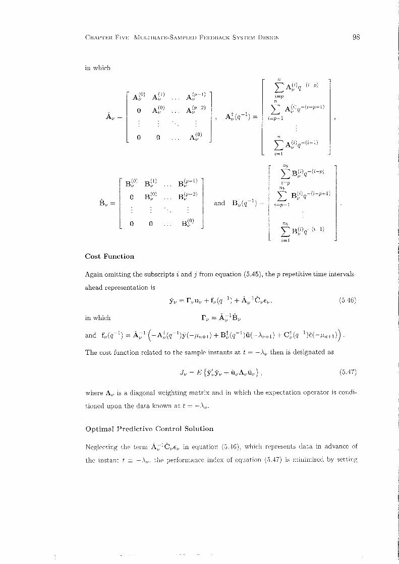
CHAPTER FIVE MULTIRATE-SAMPLED FEEDBACK SYSTEM DESIGN
in which
n
rA~O: AP) A}f-l)
L ASi)q-(i-p )
i=pn
Au"'"'ASO) A}f-2)
At(q-l) =L ASi)q-(i-p+l)
li=p-l
0 0 ASO) nL ASi)q-(i-l)
i=1
nb
BSO) BS1) B}f-l)
L BSi)q-(i-p )
i=pnb
:l3u=0 BSO) B}f-2)
Bt(q-l) = L BSi)q-(i-P+l)
and i=p-I
0 0 BSO) nb
jL BSi)q-(i-l)
i=1
Cost Function
98
Again omitting the subscripts i and j from equation (5.45), the p repetitive time intervals
ahead representation is
in which
(5.46)
The cost function related to the sample instants at t = -Au then is designated as
(5.47)
where Au is a diagonal weighting matrix and in which the expectation operator is condi-
tioned upon the data known at t = -Au.
Optimal Predictive Control Solution
Neglecting the term A~lcuEu in equation (5.46), which represents data in advance of
the instant t == -Au. the performance index of equation (5.47) is minimised by setting

CHAPTER FIVE MULTIRATE-SAMPLED FEEDBACK SYSTEM DESIGN 99
8Ju/8uu = 0, whence the optimal sequence of controls throughout the prediction horizon
IS
(5.48)
The "optimal" predictive control law at t == - Au for the lh control then represents the
last row of equation (5.48), namely,
(5.49)
Repeating the procedure described above for each control Uj ( - Au), j = 1,2, ... , l, for each
relevant sampling instant Au E {O, AI, ... , A1>}, the overall predictive control law is given
by
(5.50)
Predictive Controller
Due to its dependency upon the white noise signal E(O), the predictive compensator cannot
be implemented directly. Correspondingly, specifying the following left-matrix fraction:
C-1( -1)8 ( -1) = 8 ( -1)c-1( -1)s; q Ce q E q q, (5.51)
in which CS c
(0) is required to be block upper-triangular, then the combination of the
control law of equation (5.50) with the "repetitive time interval index-dependent" plant
description of equation (4.34) yields the controller
where
(5.52)
Remarks
1. Generalisation of Approach
Expression (5.39a) represents the case in which a control at t == - A1/ directly precedes and
immediately follows, measurements at t == - JLrc and t == - fLrc+1 respectively. As indicated
by the following interlacing of sampling instants:
(5.53)

CHAPTER FIVE l'vIULTIRATE-SAMPLED FEEDBACK SYSTEM DESIGN 100
when two or more controls are applied in succession, the methodology described in this
section remains unaltered until equation (5.49), at which juncture the "optimal" predictive
control laws at the sample instants t == '\v-(+I, t == -'\v-(+2,"" t == -'\v, are specified
to constitute the last ( rows of equation (5.48).
Now consider the situation in which, instead of expressions (5.39b), the time-delay d is
given by
d = oN + d; dE [0, N - 1]. (5.54)
In this event, the matrices BSO), BP), ... ,Bt-I) , in equation (5.45) vanish and the ele
ments in BSv) relating an output Yi(uN - f.L()) to Uj( -,\v) are zero for
f.L() + d > ,\v· (5.55)
where
Thus, although penalised within the cost function of equation (5.47), since the outputs at
the sampling instants t == ii N - f.L(), t == uN - f.Le+I,···, t == -f.LK.' are unaffected by the
controls Uj (-'\v), they are irrelevant with regard to computing the predictive controller.
In such circumstances, it may be necessary to increase the parameter p by u or u + 1 to
compensate.
2. The 5150 Case
The matrices A v , B; and C; determining the p repetitive time intervals-ahead represen-
tation are obtained from equations (3.68) and (3.73) and by observing that the subscript
1/ corresponds to the index l (E [O,L - 1]) in equation (4.40). Replacing l by j to avoid
confusion with the matrix B[ in equation (3.68), equation (5.42) becomes
Aj(q-l)YM((M - mj)L) = Bj(q-l)ud(L - j - I)M) + Cj(q-l)EM((M - mj)L), (5.56)
Aj(q-l) = p\~f-mj)(q-l)AM(q-l) (qP~7j)(q-l)),
with Cj(q-l) defined similarly, and
Bearing in mind the comments pertaining to equation (4.40) and the above discussion
regarding the application of several controls in succession, in the event when L > iII and,
therefore,
mj-E,+l = mj-E,+2 = ... = Tnj, (5.57)

CHAPTER FIVE l'vIULTIRATE-SAivIPLED FEEDBACK SYSTEl\\ DESIGN 101
it suffices to specify equation (5.56) for j and mj alone. Moreover, when mj = M, it
is convenient to combine this particular model with that acquired for mj = °by adding
IiM (= N) to each matrix superscript and vector argument. As a result, equation (5.56)
need only be evaluated for j = 0,1, ... , J - 1, where
J = min(L, M). (5.58)
In the FOS scenario, the model corresponding to equation (5.42) results by observing
that d ::::: 1 and consequently defining bl in equation (3.75) as
whence (5.59)
Accordingly, specifying
in equation (3.76), the corresponding Frs representation is
5.4 Illustrative Example - Predictive Control
(5.60)
The derivation of a predictive controller for the system denoted as NIl is considered in
this section. Whilst the primary objective is to demonstrate the principles established in
section 5.3, it is instructive to compare the structure of the predictive control law with its
LQG counterpart, acquired in section 5.2.
Predictive Controller Derivation
The initial stage in the derivation procedure concerns the designation of the sampling
instants -ILl<, -/\V' -111<+1 and -Av + l for each control applied during the repetitive time
interval. Bearing in mind that the system vectors are
y(o) = [.7JdO) .712(0) Y2(-2) Y2(-4) rand u(O) = [u(O) u( -3) r

CHAPTER FIVE MULTIRATE-SAMPLED FEEDBACK SYSTEM DESIGN 102
then, addressing the control u(O), the sampling instants are interlaced thus (see (5.39a)):
where
(5.61)
The vectors y(N -/J'K+l) and u(N -Av+d then are specified respectively as (see (5.40a,b))
and
y(N - tLK+d = y(6) = [Yl(6) Y2(6) Y2(4) Y2(2) r
u(N -Av+d = u(3) = [u(3) u(O) r,which are related to y(O) and u(O) via the permutation matrices (see (5.41a,b))
(5.62a)
(5.62b)
P~N-"''')(q-'l ~ q-'14 and P),N-A'+'l(q-') cc [qO, ~] (~p;l)(q"l)
Using the subscript v = 0, the AO(q-l) and BO(q-l) matrices specified in equations
(5.43a,b) are given (via equation (5.42)) by
(5.63)
1 0 0 0 -a6 0 0 0
0 1 -2 0 0 0 0 0A(O) - -a A(l) -where o - and o -0 0 1 -')
0 0 0 0-a-
0 0 0 1 0 -2 0 0-a
(1 + a + a2)b1 (a3 + a4 + a5)b
1
B (-1) -B(O)- (1 +a)b2 0and o q - 0 - (5.64)
b2 ab2
0 (1 + a)b2
Notice that, with a6 and a2 replaced with -Cl and -C2, respectively, CO(q-l) is defined
similarly to AO(q-l). Selecting the parameter p as 3, the vectors Yo and uo are (see
(5.44a,b))
Yo = [y'(18) y'(12) 5"(6) rand 110 = [U'(15) u'(9) u'(3) r
whereas the matrices in equation (5.45) are:
A(l)o
A(O)o
o
At 0-

CHAPTER FIVE l'vIULTIRATE-SAMPLED FEEDBACK SYSTEM DESIGN
with Go and Cb arranged accordingly, and
103
Repeating the above procedure for the control u( -3), the resultant sampling instants
are ordered thus:
where
(5.65)
The permutation matrices relating
and
y(N - f.Lr<+d = y(2) = [Y2(2) Yl(0) Y2(0) Y2( -2) ]'
u(N - Av+d = u(O) = [u(O) u( -3) ]'
(5.66a)
(5.66b)
to, respectively, y(O) and u(O), are
0 1 0 0
p~N-P."+l)(q-l) = 0 0 1 0 (= pi1)(q-l)) p(N-.\v+d(q-l) =Iand u 2,
0 0 0 1
q-l 0 0 0
whence, with the subscript v = 1, the matrices in equations (5.43a,b) are:
1 0_.)
0 0 0 0 0-a-
A(O) - 0 1 0 0 A(l) - 0 -a6 0 0in which 1 - and 1 -
0 0 1 -? 0 0 0 0-a-
0 0 0 1.,»
0 0 0-a-
with C1(q-l) specified likewise, and
B 1(q-l) = B;O) + B;l)q-l.
(1 + ii )b2 0 0 0
B(O) - 0 (1 + a + a2)b1 B(l) - (0
3 + 01 + a.5)b 1 0
where 1 - and 1 -
0 (1 + ii)b2 0 0
0 b2 iib2 0
(5.67)
(5.68)

CHAPTER FIVE MULTIRATE-SAMPLED FEEDBACK SYSTEM DESIGN
The vectors YI and UI are (see (5.44a, b))
YI = [Y'(14) y'(8) y'(2) J' and UI = [U'(12) u'(6) u'(O) J',
104
whereas the matrices Al and At (and (;1 and ct) are arranged in accordance with,
respectively, Ao and Ab. In this instance, the matrices B1 and Bt also are organised
similarly to, respectively, Ao and Ab.
Numerical Example
Using identical values as in section 5.2, namely,
al = a = 0.9615, b1 = 0.0385, a2 = a = 1.04 and b2 = 0.04,
the last rows of equation (5.48), obtained by minimising Jv , v = 0,1, for weighting matrices
Ao = 0.037516 and Al = 0.37516 ,
with respect to the 3 repetitive time intervals-ahead representation of equation (5.46),
yields the following control laws (see (5.49)):
with
and
and
with
and
RO(q61 )U(0) = -s~o(q-l)y(O) + S~o(q-l)E(O),
RO(q6 1) = 1,
Syo(q-l) = [ -0.1020 5.3888 0 0 J'sco(q-l) = [ -0.0624 3.6185 0 0 J',
R1 (q6 1)U(- 3) = -S~1(q-l)y(-4) +S~1(q-l)E(-4),
R 1(q61
) = 1+0.1212q63,
SYI (q-l) = [2.4359 0.2203 0 0 J'[ 0 ]
'Sq (q-l) = 1.6357 0.1349 0
(5.69a)
(5.69b)
Eliminating the terms dependent upon the white noise sources via the combination of
equations (5.69a,b) with the open-loop model and evaluation of the left-matrix fraction in
equation (5.51), the predictive controller is specified by (see (5.52))
[
1 - 0.1272q-l 04339 ]
n, = 0.3271q-l 1 _ 0·.29·27q-I

CHAPTER FrVE MULTlRATE-SA!\lPLED FEEDBACK SYSTEM DESIGN 105
and[
-0.0396So =
0.0826q-1
1.7703
0.7093q-1
1.2857
0.5152q-1
0.9662 lI
0.8002 JScaling the entries within the corresponding polynomial matrices in the LQG regulator
derived in section 5.2 such that the diagonal entries in Ro(O) are 1, whence
-I [1 0.2074q-1ROLQC(q ) =
0.5136q-1 ]/
0.3640
1 - 0.1599q-1
and[
-0.0686
0.0512q-1
1.3160
1.1577q-1
1.0036
0.8408q-1
0.8189 ] /
1.4182
it will be observed that the predictive controller bears a marked resemblance, both in
terms of its structure and numerical values. The latter aspect is confirmed by noting that
the phase margin is
PM = 48.4389° (d. 48.4214°),
and that the gain margins are
GMu = +15.0200dB (d. + 16.4479dB) and GMl = -8.1083dB (d. - 8.3904dB).
While the choice of the parameters determining Ao and Al in the above example engender
satisfactory results, in general it is by no means clear how appropriate weighting matrices
A v should be selected. Accordingly, this topic constitutes a possible future research area.
5.5 Enhancement of Design Methods
The optimal and predictive control design approaches described earlier in this chapter may
prove to be somewhat restrictive in certain practical applications without modification. Of
particular significance in this respect is the desirability of introducing integral action within
the multirate-sampled controller to ensure the asymptotic tracking of step changes in
reference signals and the possible incorporation of dynamic weighting within performance
indices as a means of producing satisfactory stability robustness. Whilst addressing both
these issues, this section additionally outlines the possible extension of the foregoing design
methods to encompass the "tracking" and "feedforward" problems.

CHAPTER FIVE l'vIULTIRATE-SAMPLED FEEDBACK SYSTEM DESIGN
Integral Action
106
The incorporation of integral action within the controller is facilitated by assuming that
the disturbance signal is drifting, thereby necessitating the use of an ARIMAX (Auto
Regressive Integrated-Moving Average-eXtended) system representation. Given that this
artifice is rarely justifiable from a physical perspective, the term "optimal controller" may
constitute a misnomer and LQG control theory then represents a design aid rather than a
genuine synthesis technique in this context. The following analysis details the procedure
involved in the MIMO case, whilst the general SISO, FOS and FIS cases are dealt with in the
sequel.
In the MIMO scenario, it is supposed that the fast-rate discretised system model is de
scribed by the ARIMAX representation
where
Y(ZN) = Zt/A-1(zA;l)B(zt/)U(ZN) + D-1(zA;l)A-1(zt:;l)C(zjVI)e(zN),
D(zjVI) = (1- zjVI) 1M .
(5.70)
Disregarding the disturbance subsystem for the present, pre-multiplication of equation
(5.70) by D(zjVl) and utilisation of the procedure summarised by equations (4.7), (4.8),
(4.9) and (4.10) yields the model:
At::.(q-l)y(O) = Lim(q-I)B(q-I)p;d)(q-I)H(q-l)u(O)
= B(q-l)p;d) Lil(q-I)H(q-I)u(O),
where the kNlkN matrix Lik(q-I) is designated generically as
(5.71)
with
and
Lik(q-l) = block diag(.6.N(q-I),.6.N(q-I), ... , .6.N(q-I)) ,
.6.K(q-l) = IK-P}P(q-I),
At::. (q-I ) = Lim(q-I )A(q-I).
Before proceeding further, it is necessary to introduce the following result related to the
W K matrices (see (3.33)):
(5.72)
where, with 1\R = N,
wt = block cliag (w;,.. w}.' ..... wk) .

CHAPTER FIVE J'vIULTIRATE-SAMPLED FEEDBACK SYSTEM DESIGN 107
in which
Consequently, it can be established from equations (4.8) and (4.9) that
(5.73)
where
and
Specifying the derivative of each control thus:
ute,)-ljLj) = (1- qZn uj(-ljLj)
= Uj( -ljLj) - Uj( -(lj + l)Lj), lj = 0, 1, ... , Lj - 1, j = 1,2, ... , l;
then, exploiting the theory developed in Chapter 3, the vector TI6. (0) comprising the control
derivatives specified throughout the repetitive time interval is, using the definitions of t::.. H
and D..K in equations (5.73) and (5.71), respectively, given by
(5.74)
Invoking equations (5.73) and (5.74) and re-instating the disturbance signal, the lifted
representation relating the fast-sampled outputs to the slow-sampled controls and fast-
sampled white-noise sources is
where
(5.75)
The overall lifted representation then is given by
(5.76)
where (A6 , B6.) are obtained from (A6.. BH",) by following the method summarised by
equations (4.11), (4.12) and (4.13), whereas C.0.E is acquired from Ate, and Ce via the
technique detailed in section 4.:3.
Bearing in mind that the matrix C AI", and polynomial ''(6. arise from equation (3.63) in
which the following substitutions are made:
(srso)

CHAPTER FIVE i'vIULTIRATE-SAMPLED FEEDBACK SYSTEM DESIGN 108
Table 5.3. Lifted ARIMAX models: scalar case.
A.6. B.6. C.6.
SISO AMAMV Li(M)A(M)B p(!d+d-l)Wt
CM",M N N N N L
FOS ANANB p(N+d-l) t C NN N w N
FIS (1 - z-l) ex ' Li(N) A(N)B p(d) "(.6.V N N N N N
(FIS)
A(K)(ZN1) f-- (1 + zN1 + ... + ZN L+ 1
) A(M)(zN1) (see (3.17));
AK(Z//) f-- (1- z-l) ex(z-l)
A(K)(zN1) f-- (1 + zN1 + ... + ZNN+l) A(N)(zN1
) (see (3.17)),
the terms .1\.6., :13.6. and (;.6. in the general SISO, FOS and FIS cases are given in Table 5.3.
Dynamic Weighting
In order to improve stability robustness or as a means of meeting performance criteria,
is often necessary to incorporate dynamic weighting within the cost function. It is pro
posed to demonstrate how this may be accomplished in multirate-sampled configurations
by focusing solely upon the MIMO LQG problem, in which the performance index, given
originally by equation (5.1), now is defined thus:
J = E {'IJ'(O)'IJ(O)} , 'IJ(O) = [ n(q-l )5'(0) ]Y(q-l )u(O)
With the matrix D specified to be the stable solution of (d. (5.3))
(5.77)
(5.78)
the optimal controller is, as beforehand, acquired from equation (5.5), where (R md , Smd,
A~d) represents the minimum degree solution of the diophantine equations
AI;Y*YCb + A*B c = D*R
B~n*nCa - A* A c = D*S.
(5.79)
(5.80)
The matrices nand Y may de derived from corresponding entities defined with respect
to the short time interval. For example, by analogy with the procedure used to engender

CHAPTER FIVE l'vIULTIRATE-SAl\IPLED FEEDBACK SYSTEM DESIGN 109
5'(0)
K
Figure 5.2. The regulator problem.
A(q~I) ((4.34)) from A(zfVI) ((4.6)) (see (4.7) (A), (4.12) (A,.) and (4.14) (A)), the
specification of an appropriate W(zfVl) will result in the weighting matrix O(q-l). The
use of a similar approach will yield Y(q-l) from some V(zfVl), although in this instance
each of the complementary operations is governed by the arrangement of signals within
the vectors 6.(0) ((4.7)), U(O) ((4.9)) and u(O) ((4.34)).
Alternative Control Problems
Thus far, this thesis has been concerned solely with the regulator problem encapsulated
by the block diagram model of Figure 5.2. Nonetheless, there are many instances in which
more sophisticated methods are required to model and control system satisfactorily. Conse
quently, focusing on the MIMO LQG approach throughout and eschewing detailed solutions,
the following analysis outlines alternative control problems which may be addressed using
the methods developed hitherto.
It can be readily shown that the regulator problem subsumes instances in which a feed
back system is driven by two or more exogenous disturbances. In this respect, consider
the discretised plant/ disturbance subsystem model
(5.81)
It is supposed additionally that the input to the digital controller is the system error signal
e(z,v), defined thus:
(5.82)

CHAPTER FIVE !vIULTIRATE-SAMPLED FEEDBACK SYSTEM DESIGN 110
and in which J.L(ZN) and r(zN) represent, respectively, measurement noise and the reference
signal. Notice that, with a slight abuse of notation, V(ZN), J.L(ZN) and ((ZN) denote m
weakly stationary discrete-time white signals with zero mean. Defining
G(N (ZN) ] = [ zr/A;; I n;= A-I [ Zr/B (5.83)
where it is supposed that each of the subsystems G pN, G VN and G(N is free of unstable
hidden models, the matrix C(zj::/) is deemed to represent the stable solution of
(5.84)
in which the diagonal mlm matrices I;f.L' I;v and I;( represent the power spectral densities
of the white noise sources.
Using the techniques detailed in section 4.1 and 4.2 to acquire, respectively, the plant
model G p and the lifted MA process C(q-I )£(0), the system defined above can be modelled
thus:
in which
e(O) = -Gp(q-l)u(O) + Gd(q-I)£(O),
Gp(q-I) = A -l(q-I)B(q-l) and Gd(q-I) = A -1(q-I)C(q-I).
(5.85)
The comparison of equation (5.85) with equation (4.35) indicates that minimisation of the
performance index (cf. (5.77))
J = E { r/(0)7](0)} ,[
O(q-I )e(O) ]7](0) = ,
T(q-I )u(O)(5.86)
will engender the optimal controller specified by the diophantine equations (5.79) and
(5.80) and the matrix fraction conversion of equation (5.5). The equivalent closed-loop
configuration therefore may be depicted as the block diagram model of Figure 5.3, in which
it will be observed that the controller K(q-I) appears in the forward path.
The "tracking" problem - namely, the requirement that the output y follows a stochas
tic reference r as closely as possible in the presence of other random disturbances - is
addressed more commonly by the "two degrees-of-freedom" controller structure schemat
ically represented for the multirate MII\IO case in Figure 5.4. Sebek (198:3) demonstrated

CHAPTER FIVE l'v!ULTIRATE-SAl\IPLED FEEDBACK SYSTEM DESIGN 111
Figure 5.3. Equivalent closed-loop configuration.
y(O)
Figure 5.4. The tracking problem.
that the polynomial solution of the minimisation of
J = E {"1' (0)"1(0) } ,[
O(q-l) (r(O) - y(O)) ]"1(0) =
Y(q-l )0.(0)(5.87)
for the plant and disturbance signals defined above produced the control law
(5.88)
where K(q-l) represents the "regulator solution" obtained previously and, specified via a
further diophantine equation, in which Kr(q-l) denotes the "reference controller".
The second major extension to the regulator problem was the derivation by Hunt and
Sebek (1989) of a solution to the "feedforward" problem, in which a separate feedforward
compensator effected the rejection of a measurable disturbance. Depicted schematically
in Figure 5.5, the vectors ill and fi denote the measurable and unmeasurable disturbances
generated by applying the white noise source w to the blocks labelled G m and G n , whereas
K f denotes the feedforward controller. The LQG control law minimising the performance
index of equation (5.77) then assumes the structure
(5.89)

CHAPTER FIVE fvIULTIRATE-SAMPLED FEEDBACK SYSTEM DESIGN
Figure 5.5. The feedforward problem.
Modified Predictive Control Solution
5'(0)
(L(O)
112
The approach utilised in section 5.3 to synthesise multirate-sampled predictive control laws
for the regulator problem can accommodate the modifications described in this section.
The following analysis accordingly describes the procedure entailed in deriving a "two
degrees-of-freedom" predictive controller that incorporates integral action.
The initial system model is acquired by invoking the permutation matrices II2 and II3
specified in equation (4.32), whence equation (5.76) may be written as
(5.90)
Introducing the signals
<pi(-L) =wi(qi/)(Yi(-L)-ri(-L)), i= 1,2, ... ,m,
in which it is assumed that each reference signal r, (-L) is known throughout the relevant
predictive interval t E [-p,,,,pN - p,,,+I], then, using the methods detailed earlier in this
section, the vector ip can be defined thus:
ip(O) = O(q-l) (5'(0) - f(O)).
The designation of the left-matrix fraction
A-I ( -1)0 ( -1) = O( -1)A -1( -1)6n q a q q 6. q
(5.91)
(5.92)
consequently warrants the definition, from equations (5.90) and (5.91), of the following

CHAPTER FIVE i'vIULTIRATE-SAMPLED FEEDBACK SYSTE1\! DESIGN
model:
113
A6n(q-1)~(O) = Oa(q-I)B6(q-1)U(O) + Oa(q-1)C6(q-1)E(O) - A6n(q-I)O(q-I)r(O).
(5.93)
For concision, using the symbols A, B, C and D to signify entities related to A6n'
OaB6, OaC6 and A6nO, respectively, the resultant p repetitive time intervals-ahead
representation (cf. (5.46)) is
(5.94)
where
f Iv(q-1) = A;;I ( -At(q-1 )O(q-1 )Y( -!LK+d + Bt(q-1 )U6( -Av+d + Ct(q-I )E(-!Lt<+I))
and f 2v (q- I) = A;;l (Dvfv + (Dt(q-1) - At(q-I)O(q-1)) rV(-!Lt<+I)).
Minimisation of the cost function of equation (5.46), in which Yv is replaced with 1pv,
consequently yields the optimal control sequence (see (5.48)) with respect to t = -Av and
ultimately, via equations (5.51) and (5.52), the overall predictive controller. Notice that,
if it is assumed that each reference signal r; (-) constitutes a unit step applied at t == - N,
it can be established readily that the vector f2v (q-I) in equation (5.96) may be described
thus:m
f 2v (q- 1) = q-1 L~Vi(q-1)ri(O).
i=l
(5.95 )
As a consequence, it is relatively straightforward to compute the optimal predictive control
law
Replacing A, Band C in equations (5.51) and (5.52) with A 6, B 6 and C 6, respectively,
the "two degrees-of-freedom" predictive controller is described by (d. (5.88))
where
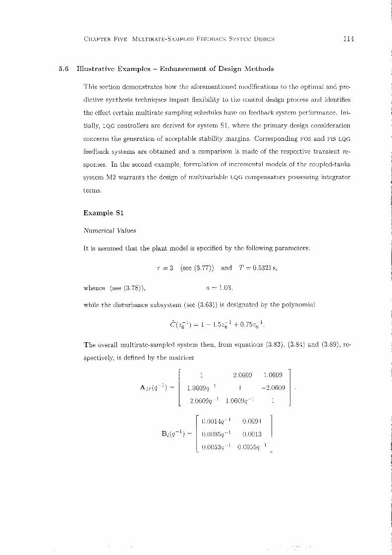
CHAPTER FIVE IvIULTIRATE-SA!'vlPLED FEEDBACK SYSTEM DESIGN
5.6 Illustrative Examples - Enhancement of Design Methods
114
This section demonstrates how the aforementioned modifications to the optimal and pre
dictive synthesis techniques impart flexibility to the control design process and identifies
the effect certain multirate sampling schedules have on feedback system performance. Ini
tially, LQG controllers are derived for system 81, where the primary design consideration
concerns the generation of acceptable stability margins. Corresponding FOS and rrs LQG
feedback systems are obtained and a comparison is made of the respective transient re
sponses. In the second example, formulation of incremental models of the coupled-tanks
system M2 warrants the design of multivariable LQG compensators possessing integrator
terms.
Example 81
Numerical Values
It is assumed that the plant model is specified by the following parameters:
T = 3 (see (3.77)) and T = 0.5321s,
whence (see (3.78)), a = 1.03,
while the disturbance subsystem (see (3.63)) is designated by the polynomial
The overall multirate-sampled system then, from equations (3.83), (3.84) and (3.89), re
spectively, is defined by the matrices
r
O.0014q-l
B1(q-l) = 0.0095q-l
0.0053q-l
1
1.0609q-l
-2.0609q-l
-2.0609 1 06091
-~.016091.0609q-l
0.
00941
0.0013
0.0055q-l

CHAPTER FIVE MULTIRATE-SAMPLED FEEDBACK SYSTEM DESIGN 115
and
-0.9009
1
0.4466q-1
0.4466 j-0.9009
1
LQG Controller Design
In the first design attempt, minimisation of the cost function of equation (5.1) for the 5I50
case (see Table 5.1) in which
yields the optimal controller Ko(q-l), specified by the matrices (see (5.4))
[
1.1881 + 0.3538q-l
-0.1793q-l
-0.1729 ]
1.1881 + 0.2233q-l
and-1 [14.2188
So(q ) =-6.8955q-l
-0.7406
-7.1062q-l
-12.1841 ] .
14.9745
The remaining matrices entailed in the derivation of the LQG control solution, namely,
Ba(q-l) and Ab(q-l) (i.e., Br(q-l) and Ar(q-l) - see Table 5.1), Bc(q-l) and Cb(q-l)
((5.2)), D(q-l) ((5.3)), Co(q-l) ((5.5)) and Rmd(q-l), Smd(q-l) and A md(q- 1) ((5.6) and
(5.7)) are listed in Appendix A.
The above controller produces "plant poles" (namely, the zeros of z2det (D(z-1))) at
z = 0.75482:jO.I716,
corresponding to a damping factor ( of 0.7533 and a natural frequency of resonance
W n of 0.6389 rad/s. The poles related to the disturbance model (given by the zeros of
z2det (Cx(z-l)), where C, represents C, C a (i.e., CM), C b or Co) are located at
z = -0.23802:jO.1802,
with associated values of ( and W n of 0.4363 and 5.208:3 rad/s, respectively. It will be
observed that the dominant closed-loop poles, specified with respect to the repetitive time
interval of T s, conform to conventional sampling rate selection criteria and are located at
positions in the z-plane which normally would be deemed acceptable in single-rate digital
feedback systems with a sampling interval of T s. Bode plots of the characteristic gain

CHAPTER FIVE MULTIRATE-SAMPLED FEEDBACK SYSTEM DESIGN 116
Q:I 10"0
I o ..:::'"0- 10
...:~ -]0
U-J0F------~----
21lO
I
~ IIlO
'"..c:0...
PM
...:'"..c:U -11lO
10"
Frequency (rad/sec)
Figure 5.6. Bode plot of characteristic gain loci - system S1.
loci related to the return ratio QL(z) (See (4.51a)) provided in Figure 5.6 reveal that the
margins of stability are
PM = 43.4273°,
GMu = +10.7914dB and GMl = -9.7223dB.
Striving to enhance relative stability, a second control design engendered by minimising
J in equation (5.77), where
produces the LQG compensator specified by
-0.0212
0.1320 + 0.0247q-' ][
0.1320 + 0.0396q-l
-0.0211q-l
and1.4797
-0.74:17q-l
-0.1132
-0.7477q-l
-1.3021 ] .
1.5404
Observing that the "disturbance subsystem poles" are invariant, the closed-loop "plant
poles" are
z = 0.7043 and z = 0.8627.

CHAPTER FIVE l'vIULTIRATE-SAMPLED FEEDBACK SYSTEM DESIGN 117
with related values of W n of 0.6588 and 0.2776 rad/s, respectively. The stability margins
in this instance are
PAl = 49.7071°,
GMu. = +11.3339dB and GM! = -9.6271dB.
FOS and FIS LQG Designs
It is instructive to examine comparable control designs for FOS and FIS sampling schedules
in which N = 6. In the former instance, minimisation of J in equation (5.1) with
B =4.
produces the control solution (p(q-l), S~(q-l)), where
and
p(q-l) = 2.8223 + 2.6392q-l + O.6111q-2
27.3859 + ll.5534q-l
14.3053 + 6.0351q-l
0.9186 + O.3875q-I
-9.3512 3.9450q-l
-14.7157 - 6.2082q-l
-15.0601 6.3535q-l
In the complementary FIS scenario, the term B in equation (5.1) is given by
and the resultant optimal controller (R(q-l), s(q-l )) is specified by
0.3353 -0.4360 0.0448 0 0 0
0 0.3353 -0.2800 0.3072 0 0
0 0 0.:335:3 -0.6414 0.:3072 0R(q-l) =
0 0 0 0.335:3 -0.6414 0.3072
O.3072q-l 0 0 0 0.3353 -0.6414
-O.6..H4q-l O.1486q-l 0 0 0 0.3353
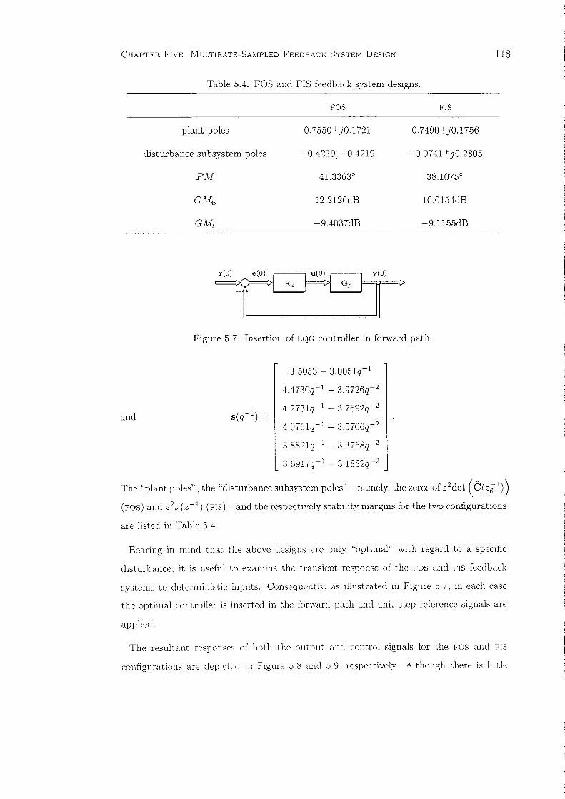
CHAPTER FrVE l'vIULTIRATE-SAMPLED FEEDBACK SYSTEM DESIGN
Table 5.4. FOS and FIS feedback system designs.
FOS rrs
118
plant poles 0.7550:':jO.1721 0.7490 :':jO.1756
disturbance subsystem poles -0.4219, -0.4219 -0.0741 :':jO.2805
PM 41.3363° 38.1075°
GMu 12.2126dB 1O.0154dB
GMI -9.4037dB -9.1155dB
Figure 5.7. Insertion of LQG controller in forward path.
and -( -1)sq =
3.5053 - 3.0051q-l
4.4730q-l - 3.9726q-2
4.2731q-l 3.7692q-2
4.0761q-l - 3.5706q-2
:3.8821q-l - 3.3768q-2
3.6917q-l - 3.1882q-2
The "plant poles", the "disturbance subsystem poles" - namely, the zeros of z2det (C(Z6 1) )
(FOS) and z2v(z-l) (rrs) - and the respectively stability margins for the two configurations
are listed in Table 5.4.
Bearing in mind that the above designs are only "optimal" with regard to a specific
disturbance, it is useful to examine the transient response of the FOS and rrs feedback
systems to deterministic inputs. Consequently, as illustrated in Figure 5.7, in each case
the optimal controller is inserted in the forward path and unit step reference signals are
applied.
The resultant responses of both the output and control signals for the FOS and FIS
configurations are depicted in Figure .5.8 and 5.9, respectively. Although there is little

CHAPTER FIVE !v1ULTIRATE-SAMPLED FEEDBACK SYSTEM DESIGN 119
15
10 15
10p=;-------,---------r-----------,
-5
III
_IOe-:= -'-- ----'- --
o IS
Time
Figure 5.8. Transient response in FOS control system.
I.S
III IS
III \
III IS
Time
Figure J.9. Transient response in FrS control system.

CHAPTER FIVE rvIULTIRATE-SAMPLED FEEDBACK SYSTEM DESIGN
15,--------,.--------.-----------,
120
'"9-'"
Oil.)
10
:5 50c
Time
10
10
15
15
Figure 5.10. Transient response in general multirate control system.
discernible difference between the two sampling strategies in terms of the behaviour of the
output signal, it is evident that control activity in the two cases differs markedly. In fact,
it has been established by Truman and Govan (2000b,c), that the FOS scheme behaves
similarly to conventional single-rate controllers implemented with sampling intervals of
either T / N s or T s in terms of the transient behaviour of both the control and output
signals.
For comparative purposes, the transient response of the general S1SO system is shown in
Figure 5.10. Notice that the overshoot exhibited in each of the output signals in Figure 5.8,
5.9 and 5.10 is caused by the phase lead introduced by the controller necessary to ensure
closed-loop stability. This problem can be circumvented by implementing a "two degree
of-freedom" control law via the approach outlined in section 5.5.
Discussion
The nature of the control signal in the F1S scheme can be explained qualitatively by
considering the first-order controller defined thus:
U.v(z.v) = KV(ZN)E(z) (c:f. (2.8) or (2.17)),
wheres
f{X(ZN) = -I' 1'>0.1 -- I'Zx

CHAPTER FIVE l'vIULTIRATE-SAMPLED FEEDBACK SYSTEM DESIGN 121
The relationship between the incremental controls U6 (-0) - namely, u( -0) - u( -0-1) (see
(5.74)) - and the error signal e(-0) during the repetitive time interval can be expressed
thus:
U6 (0) = rU6 (-1) + s (e(O) - e(- N)) :
U6(0) = rud -0 - 1), 0 E [1, N - 1]. (5.98)
(5.99)
Consideration of the magnitude of the control increments, namely, IU6(-0) I, 0 E [0, N - 1],
in equation (5.98) indicates that the control signal may exhibit a noticeable change at each
"slow-rate" sampling instant kT s, following which, provided r < 1, it will tend to decay
exponentially.
The FOS LQG control law is specified by the "implicit" pulse-transform/pulse-transfer
function relationship
U(Z) = Z {KN(zN)EN(zN)} (cf. (2.10) or (2.18) and (2.19)),
where, by comparison of the relevant entries in Table 5.1 and equations (4.43) and (4.50),
1 -:=.(N) I
( )_ S(ZN)C (ZN)
KN zN - p(r1)
The inherent anti-aliasing nature of the FOS optimal compensator may be demonstrated
by considering the i th factor of the polynomial C(N)(ZNI) , namely, C;N)(ZNI
) , which, if
Ci (zN1) = 1- CZN
1, is given by ((3.17))
C-:=. (N)( -1) 1 -I N-l -N+li zN = +czN + ... +c zN .
Thus, if C is real and close to unity, then C;N) (zN1) will resemble the so-called "comb
filter" characteristic of the discretised zero-order hold HN(ZN) (see (3.45)), namely,
(N)(7 ) _ (N)(~-I) _ 7- 1 7-N +1HN ~N - H "'N - 1 + ~N + ... + ~N .
Consequently, if one or more zeros of <~,cC(z;~/) lie in proximity to (1, 0) and N is suf
ficiently large (e.g., N 2: 8), C(zN1) will act as a low-pass FIR (finite impulse response)
filter, significantly attenuating frequency components of the output signal Y (ej wT IN) out
side wE [0,w s / 2). As discussed by Truman and Govan (2000b,c), this low-pass character
istic suppresses high-frequency noise signals, albeit at the expense of introducing a certain
degree of phase lag. Finally, it has been established by Truman and Govan (2000a) and
Truman and Govan (20(H) that the FOS predictive compensator shares this property.

CHAPTER FIVE MULTIRATE-SAMPLED FEEDBACK SYSTEM DESIGN
Example M2
122
This example concerns the design of feedback systems for the coupled-tanks model M2.
The design objectives simply require that there should be zero steady-state error to step
changes in the reference signals and that the closed-loop poles should have natural fre
quencies of resonance in accordance with the sampling schedule deployed. The strategy
adopted aims to yield relatively low-order controllers by presupposing that it is justifiable
in this instance to simplify the disturbance subsystem model such that all "C's" are, in
fact, identity matrices, thereby resulting in the use of "ARIX" representations throughout.
Initially, a lifted ARIX model is acquired, following which predictive and LQG compensators
are derived when the sampling ratio N is 3. The LQG design then is repeated for a scenario
in which N is increased to 8.
Lifted ARIX Model
The lifted time-domain representation of the discretised plant G p N (ZN) is given by equa
tion (4.10), whence,
where
A(q-l)y(O) = BH(q-l)ii(O),
y(0) = [ y~ (0) y~ (0) ] I ,
u(O) =[UI(O) u~(O) J' (= [UI(O) U2(0) 11,2(-1) u2(-2) J'),
(5.100)
, 1 [ 13 - aIp~I) -a2 I3 (1) ] '-1 [ b,W:3q-1 -b2P~I)]A(q- ) = (I) and BH(q ) = -1 ( .
-a3 P 3 h-a4P3 b3w 3q b4P31
)
The pre-multiplication of A(q-I) and BH(q-l) by Li2 (q- l ) ((5.71)) produces
where
and
(5.101)
The overall lifted ARIX model is obtained via the following procedure.

CHAPTER FIVE fvIULTIRATE-SAMPLED FEEDBACK SYSTEl\I DESIGN
(i) The vector Yr(O) and permutation matrix III are defined thus:
Yr(O) = 111y(0), Yr(O) = [y'(O) Y~]"
where
123
((4.11))
y(O) = [Y1(0) Y2(0) Y2(-1) Y2(-2)]' and Ye=[Y1(-1) YI(-2)]';
(ii) the matrices Art>. and B,t>. then are given by (see (4.12)):
where
1 -a2 a2 0
0 1 -(1 + a4) a4A1 =
a3q-1 a4q-1 1 -(1 + a4)
-I -(1 + a4)q-1 a4q-1 1-a3q
-(1 + ci) a1
-a3 a3
0 -a3
a3q-l 0
-a2 a, ]
[a,:'-(1;aJl ] ,
-a2 'A4 =
0
[ a,q-1 0A3 =
-(1 + a1)q-1 -1a2q
b1q-1 0 -b2 0
b3q-1 0 b4 0B1 =
b3q-l 0 0 b4
b3q-l b!q-l 0 0
[
b -1and B 2 = 1q
b1q-l
o
(iii) inserting the values for the parameters a; and bi , i = L 2, 3, 4 given in section 4.5
and acquiring the left-matrix fraction A121A24 (see (4.13)), the relevant model is
given by (d. (5.76))
(.5.102)

CHAPTER FIVE MULTIRATE-SAMPLED FEEDBACK SYSTEM DESIGN 124
where
and
1 - 0.7320q-l -0.0552 -0.0497 -0.0448
-0.1000q-I 1 -0.7506 -0.0061Ae. =
-0.1110q-l 0 1 -0.7506
-0.1232q-l -0.7438q-l 0 1
0.1288q-l -0.0031q-l -0.0039 -0.0035
0.0144q-l -0.00043q-l 0.1297 -0.00048Be. =
0.0091q-l -0.00048q-l 0 0.1297
0.0033q-l 0.1297q-l 0 0
(iv) observing that y(O) and u(O) are identical to, respectively, 5'(0) and U(O), then the
relevant model is given by
where
(5103)
The representation of equation (5.103) now is used to derive predictive and LQG com
pensators for the regulator problem considered in section 5.1 and 5.3. It is envisaged that
acceptable transient responses will result by placing these controllers in the forward path
of the feedback loop (see Figure 5.7) and it is therefore considered unnecessary to acquire
the "two degrees-of-freedom" control laws described in section 5.5.
Predictive Control Design
The parameters f..lK' f..lK+l, Av and AV+l required to designate the predictive controller are
defined for each of the relevant control sampling instants t == 0, t == -1 and t == -2 by
expressing (5.39a) in each instance as follows:
The relevant values are given in Table 5.5.
Choosing p to be 4, the matrices iL, At, Bv and Bt, LJ = 0, L 2, specifying the model

CHAPTER FIVE MULTIRATE-SAMPLED FEEDBACK SYSTEM DESIGN
Table 5.5. Parameters determining predictive controller.
instant /-l-K Av /-LK+I AV+I
0 -1 0 0 1
-1 0 1 1 2
-2 1 2 2 3
125
of equation (5.45) are organised thus:
ASO) AP) (2)0A v
Av =0 ASO) AP) AS2
)
0 0 A(O) AP)v
0 0 0 ASO)
o
oAS2
)
A ( l ) I. A(2) -1v' v q
BSO) BP) 0 0
Bv =0 BSO) BP) 0
0 0 BSO) BP)
0 0 0 BSO)
Notice that, since
and Bt =v
and 1/=0,1,2,
then, from equations (5.46) and (5.47), the predictive control law is not influenced by the
disturbance subsystem.
Minimising the cost function of equation (5.46), in which the vector uv comprises the
control derivatives Ui6. (.) and the weighting matrices are
Ao = diag (0.005, 0.75, 0.75. 0.75),
and Al = A 2 = diag (0.1, 10, 10, 10),
and following the procedure encapsulated by equations (5.48), (5.49), (5.50) and (5.51),
the predictive controller is given by
(.5.104)

CHAPTER FIVE MULTIRATE-SAMPLED FEEDBACK SYSTEM DESIGN
where
126
0.0195 - 0.0108q-l 0.0270 - 0.0051q-l
0.1509 - 0.0021q-l 0.1826 - O.OOlOq-l
1 + 0.2083q-I
0.0359q-l
0.0067q-l
0.0l52q-l
0.0345q-I
1 + 0.2071q-l
-0.4533q-l
0.1069q-l
1
-0.2683q-l
0.0056
1 + 0.000075q-l
1.8644 - 1.1915q-l 0.3596 -0.3757 -0.0730
So(q-l) =0.2728 - 0.2335q-l 1.7548 -1.2176 -0.0143
and0.0641q-l 2.5898q-l 3.5539 -6.1407
-4.2243q-l 1.5296q-l -0.0174q-l 2.9416
LQG Control Design
The LQG design results by minimising
J = E {v' (O)y(O) + u~ (0)3U6 (O)} , (5.105)
where
for the plant specified in equation (5.103). The matrices B a , A b, ((4.35)), D ((5.3)), and
R6 m d
and Smd ((5.6) and (5.7)) determining the optimal control solution are provided in
Appendix B. Scaled as in Example Sl , the matrices defining the LQG controller are:
1 0.0523 -0.0320 -0.0069
R 6 o(q-l) =0 1 -0.0050 -0.0011
0.0430q-l -0.0125q-l 1 - 0.0048q-l -0.0247 - 0.0010q-l
0.0518q-l -0.0151q-l -0.0058q-l 1 - 0.0013q-l
0.2828q-I - O.2423q-2 0
0.3c176q-l - O.2919q-2 -1.8095q-l
and
2.4607 - 1.6174q-l
0.2753 - 0.2519q-l
0.6550
2.5502
-0.7748 0
-1.7057 0
2.7168 -1.8748
o 2.6485
Cotnperisou of Designs
A comparison between the predictive and LQG designs can be made from the data provided
in Table 5.6. Given the similarities between the values of the coefficients of polynomials

CHAPTER FIVE MULTIRATE-SAI\IPLED FEEDBACK SYSTEM DESIGN
Table 5.6. Comparison between predictive and LQG designs.
predictive LQG
Wn 1.8333, 7.9067 2.6025, 7.6838
( 0.6817, 0.8588 0.8252, 0.8252
k l 7.1452 6.5772
k2 4.0801 6.1332
k 3.5900 5.7805
127
within respective elements of the matrices Rc,.o and So governing the two control solutions,
the corresponding proximity of the dominant closed-loop poles is not surprising. A measure
of stability robustness is provided in each instance by the parameters k 1 , k2 and k which
denote, respectively, the permissible increases in the gains of loop 1 and 2 individually
and both loops simultaneously that guarantee closed-loop stability.
LQG Design: N = 8
In this scenario, the performance index to be minimised is
where
J = E {y'(o)y(o) + u~(0)2uc,.(0)},
2 = 19 .
(5.106)
The closed-loop "poles" resulting from this design are positioned at locations in the z-plane
corresponding to
W n j = 2.5843 rad/s and (1 = 0.8160;
W n o = 20.6400 rad/s and (2 = 0.8159.
thereby justifying the sampling strategy. The feedback system remains asymptotically
stable for the following values of 1.: 1 . 1.:2 and 1.::
1.: 1 E (0,6.8572]' 1.:2 E (0.5.3922]. and k E (0.5.:3820].
The resultant controller (R6 o . So) may be separated into two components:
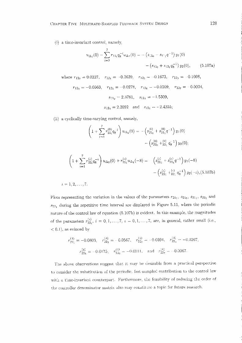
CHAPTER FIVE MULTIRATE-SAMPLED FEEDBACK SYSTEM DESIGN
(i) a time-invariant control, namely,
7
UL1l (0) + L rI2;qiiUL12 (0) = - (SIlo + sl I1q-I) u, (0)i=O
128
(5.107a)
where r120 = 0.0227, r121 = -0.2639, rl22 = -0.1673, r123 = -0.1008,
r124 = -0.0563, r125 = -0.0278, rl26 = -0.0109, r127 = -0.0024,
S110 = 2.3761, SIII = -1.5309,
S120 = 2.2092 and S121 = -2.4255;
(ii) a cyclically time-varying control, namely,
(1+ t ,\~:q8i) "6, (0) ~ - (,\~o 4 s\~), q-I) YI (0)
- (S~~~ +~~)1 qi1)
Y2(0);
L=I,2, ... ,7.
Plots representing the variation in the values of the parameters r210' S210' S21l' S220 and
S221 during the repetitive time interval are displayed in Figure 5.11, where the periodic
nature of the control law of equation (5.107b) is evident. In this example, the magnitudes
of the parameters r~~i' i = 0,1, ... ,7, L = 0,1, ... ,7, are, in general, rather small (i.e.,
< 0.1), as evinced by
(4) (4) (4) (4)1'221 = -0.0803, 1'222 = -0.0567, r 223 = -0.0394, 1'22 1 = -0.0267,
.(4) _ 0017"T225 - -. 0,J 4 l _
l225 - -0.0111. and r~;~ = -0.0067.
The above observations suggest that it may be desirable from a practical perspective
to consider the substitution of the periodic, fast-sampled contribution to the control law
with a time-invariant counterpart. Furthermore, the feasibility of reducing the order of
the controller denominator matrix also may constitute a topic for future research.
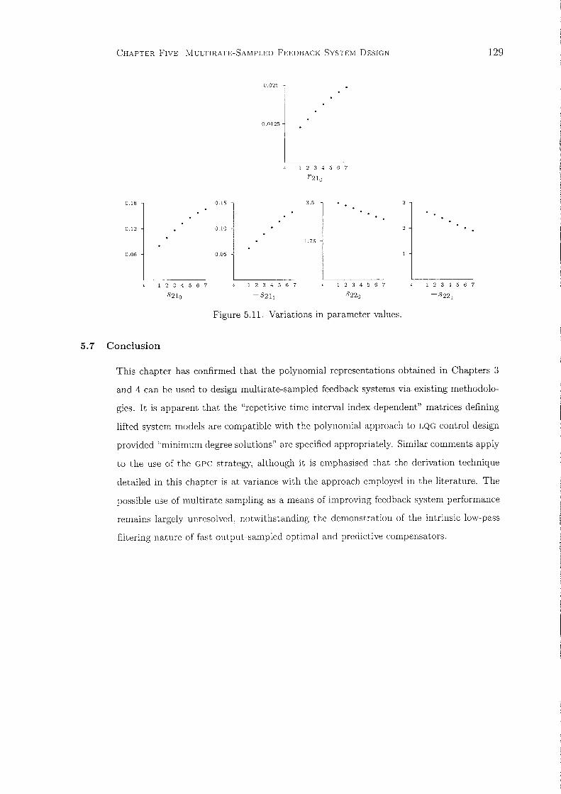
CHAPTER FIVE l'vIULTIRATE-SAMPLED FEEDBACK SYSTEM DESIGN 129
0.02.5
0.0125
1 2 3 4 567
r210
0.18
0.12
0.06
1 2 3 4 567
8210
0.15
0.10
0.05
1 234 567
3.5
1.75
1234567
8220
1 2 3 4 5 6 7
- 822 1
5.7 Conclusion
Figure 5.11. Variations in parameter values.
This chapter has confirmed that the polynomial representations obtained in Chapters 3
and 4 can be used to design multirate-sampled feedback systems via existing methodolo
gies. It is apparent that the "repetitive time interval index-dependent" matrices defining
lifted system models are compatible with the polynomial approach to LQG control design
provided "minimum degree solutions" are specified appropriately. Similar comments apply
to the use of the GPC strategy, although it is emphasised that the derivation technique
detailed in this chapter is at variance with the approach employed in the literature. The
possible use of multirate sampling as a means of improving feedback system performance
remains largely unresolved, notwithstanding the demonstration of the intrinsic low-pass
filtering nature of fast output-sampled optimal and predictive compensators.

CHAPTER SIX
CONCLUSION
This thesis has established the principles and methods entailed in the modelling and
analysis of multirate sampled-data systems utilising a transfer function-based framework,
commonly referred to as the polynomial equations approach. Moreover, it has been demon
strated that the proposed methodology, which affords dual time- and frequency-domain
interpretations, facilitates the synthesis of multirate-sampled feedback systems via the
minimisation of quadratic performance criteria, thereby proffering an alternative to the
state-space control design techniques customarily employed in this context.
The principal theoretical developments and contributions contained within the thesis
may be summarised thus:
Chapter 2
The theoretical foundations described in Chapter 2 governing the proposed modelling
approach constitute the frequency and switch decomposition procedures that were intro
duced in the 1950's. The use of an illustrative example clearly highlighted the problems
associated with multirate-sampled systems analysis using either decomposition. However,
bearing in mind the intuitive appeal that transfer function models hold for many control
practitioners, it was apparent that there existed scope for incorporating the principles
underpinning the decomposition techniques within a modern control context, thereby ex
ploiting available computer-aided control system analysis/design packages.
Chapter 3
The assimilation of the decomposition procedures within the polynomial equations ap
proach was detailed in Chapter 3, where pulse-transform/transfer function analysis and
the insertion of fictitious fast-rate sampling switches and a zero-order hold were used to
separate a SISO multirate-sampled configuration into "discretised plant" , input and output
subsystems. The definition of certain backward-shift operators then warranted the inter-
130

CHAPTER SIX CONCLUSION 131
pretation of the plant model as specifying sets of difference equations at particular sam
pling instants throughout one cycle of the sequence of sampling operations. Subsequently,
a systematic means of arranging the relevant cyclically time-varying difference equation
model in matrix-vector format was established, with care taken to emphasise the algebraic
properties linking polynomials emanating from pulse-transfer functions with their corre
sponding polynomial matrix representations. The introduction of two non-square block
diagonal permutation matrices facilitated the extension of the basic modelling approach to
encompass the switching operations related to the zero-order hold of the input subsystem
and the sampling rate conversion imposed by the output subsystem.
Observing that the above approach is closely related to the time-domain-orientated
switch decomposition technique, attention then focused upon the derivation of corre
sponding frequency-domain models of each of the three subsystems, in addition to the
transformation matrices linking vector-valued variables in each domain. The modelling of
stochastic disturbances via the proposed methodology was addressed by invoking the fre
quency decomposition of the spectral densities of a random variable sampled at different
rates, while compatibility of the related sampling rate with that of the output subsys
tem was specified via an ensuing spectral factorisation. The remainder of Chapter 3 was
devoted to the amalgamation of the individual subsystem descriptions into left- and right
matrix fraction representations, designated alternatively with respect to the time- and
frequency-domains. Thereafter, polynomial models were derived for each of the "special
cases" of fast input- and fast output-sampled systems. The chapter concluded with a
simple numerical example that illustrated the foregoing techniques.
Chapter 4
The formulation of polynomial descriptions of multirate-sampled multivariable configu
rations was dealt with in Chapter 4. Utilising a conceptually-identical strategy to that
employed in the SISO case, the chief distinguishing feature ofthe ;-"IIIvIO scenario involved the
necessity to predicate all ensuing topological operations on a left-matrix fraction model
of the discretised plant pulse-transfer function matrix. Consequently, the strong alge
braic relationships obtained between polynomials and their related polynomial matrices
in Chapter 3 have no counterparts in the general I-input/ln-output case. :"evertheless.

CHAPTER SIX CONCLUSION 132
the procedure entailed in acquiring a left-matrix fraction description of the multivariable
system was straightforward, albeit requiring a matrix fraction conversion, whereas the
derivation of the compatible stochastic disturbance subsystem description necessitated a
matrix-valued spectral factorisation.
The key issue of causality was addressed by designating a so-called "index-dependent"
time-domain model in which the elements within system vectors were arranged in accor
dance with their chronological order with regard to the sampling sequence. It was therefore
possible to ascribe specific structures to each of the polynomial matrices determining the
overall system representation and to extend this principle to its right-matrix fraction al
ternative. Hitherto neglected, similar considerations were applied to obtain corresponding
models of both multivariable and scalar multirate-sample digital controllers. Following
an examination of the criteria available for gauging the stability robustness of rnultirate
sampled configurations, an illustrative example summarised the principles established in
this chapter.
Chapter 5
Since the foregoing theoretical developments assist only the analysis of multirate-sampled
systems, the objective of Chapter 5 was to investigate the incorporation of the polynomial
modelling methodology within established control system design procedures. Accordingly,
arguably the two most popular synthesis techniques - LQG and predictive control - were
considered to be suitable vehicles in this respect. With the proviso that the structures
of the relevant matrices are designated via the criteria described in Chapter 4, it was
found that the polynomial modelling methodology was entirely compatible with the LQG
design approach, in which the optimal solution is specified via coupled diophantine equa
tions. The method adhered to in the generalised predictive control approach involved
the derivation of individual control laws at each of the control signal sampling instants
within the overall sampling sequence and subsequently combining these. Once again, pro
vided causality issues were addressed by utilising "index-dependent" matrix structures,
no significant theoretical problems emerged. Subsequently, means of introducing integral
action and engendered "two degrees-of-freedom" controller structures were outlined. The
general principles concerned in each instance were demonstrated wit h the aid of numerical

CHAPTER SIX CONCLUSION
examples.
133
While it can be stated that there are no theoretical pitfalls related to the design method
ologies discussed in this chapter, certain practical problems remain. Specifically, in com
mon with the single-rate case, a systematic means of choosing appropriate dynamic weight
ing polynomials/polynomial matrices within the cost functions specifying the multirate
LQG control problem remains elusive. A further difficulty relates to the selection of the
control weighting parameters within the performance index of the predictive methodology,
where an evaluation of their suitability can only be ascertained following the computation
of the overall multirate-sampled control law and an evaluation of the resultant closed-loop
pole locations.
The issue of whether multirate sampling can enhance feedback system performance was
not a major consideration in this thesis. Nonetheless, the use of polynomial models has
revealed that the flexibility borne by the additional controller numerator parameters in
"fast output-sampled" feedback systems designed via either the optimal or predictive
control approaches manifested itself in a low-pass FIR filter structure. Leaving overall
performance relatively unaffected, the complementary "fast input-sampled" mechanism
was shown to engender idiosyncratic control action. In conclusion, however, it appears
likely that the imposition of alternative multirate sampling schedules can improve certain
aspects of control performance only at the expense of others. Furthermore, "rules-of
thumb" governing sampling interval choice in single-rate systems accordingly apply to the
period of the sampling sequence in the multirate case.
The work contained in this thesis highlights several areas for possible further research.
For example, it is of interest to note that, although the optimal and predictive multirate
controllers are periodic with respect to the sampling cycle, thereby raising the prospect
of implementational difficulties, their parameters do not vary significantly in certain cir
cumstances. This phenomenon suggests the feasibility of synthesising time-invariant com
pensators that emulate their cyclical counterparts. Since polynomial descriptions are
conducive to system identification via parametric models, there exists the possibility of
designing self-tuning control systems that. as discussed in the Introduction, incorporate
fast output-sampling to simulate full state-feedback. Such adaptive systems then may pos-

CHAPTER SIX CONCLUSION 134
sess greater flexibility in terms of control design than conventionally sampled self-tuners.
Other topics worthy of further consideration include the facility of addressing nonlinear el
ements within the predictive control problem formulation, thus yielding an overall control
law via the combination of the solutions of a set of constrained optimisation problems, and
improved techniques for assessing the stability robustness of multirate-sampled multi-input
multi-output configurations.
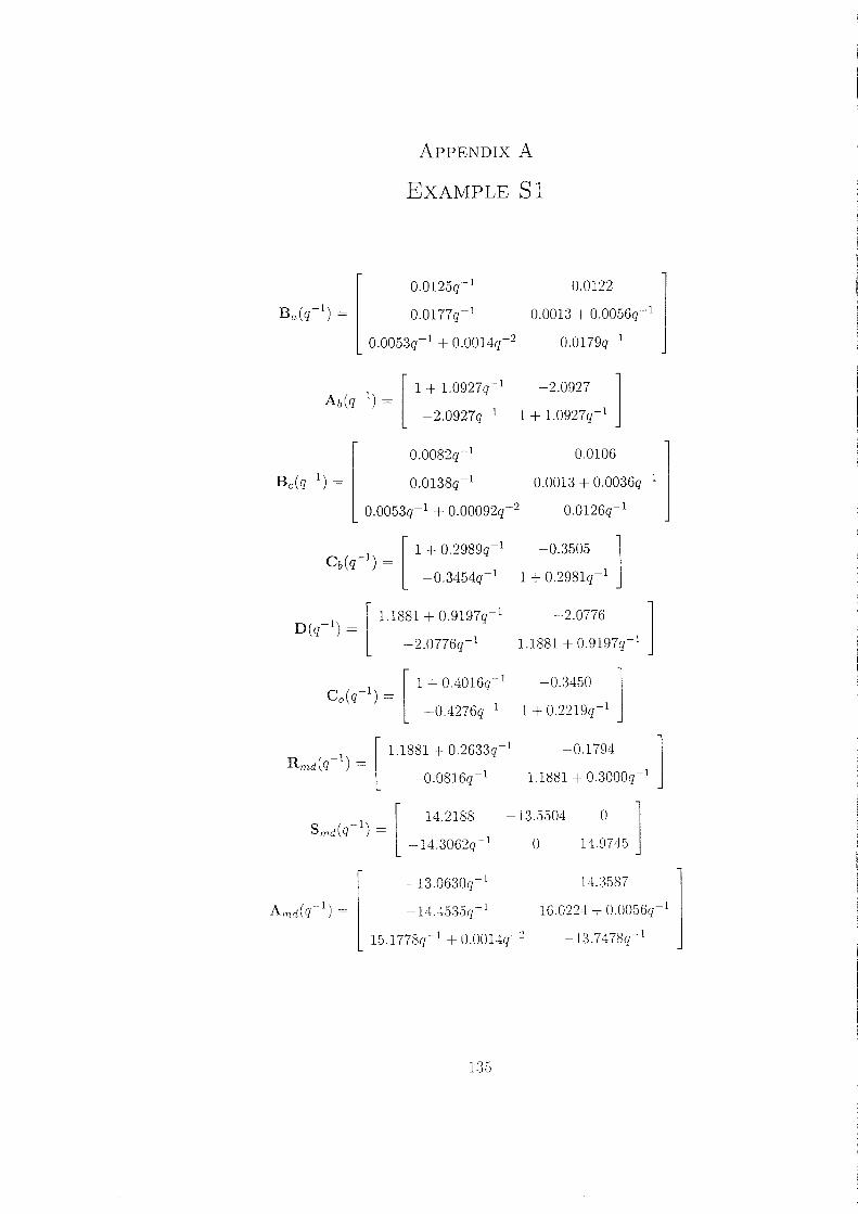
ApPENDIX A
EXAMPLE 81
[
0.0125q-1 0.0122]
Ba(q-1) = 0.0177q-1 0.0013 + 0.0056q-1
0.0053q-1 + 0.0014q-2 0.0179q-1
1 [ 1 + 1.0927q-1 -2.0927 ]Ab(q- ) =
-2.0927q-1 1 + 1.0927q-1
[
0.0082q-1 0.0106 1Bc(q-1) = 0.0l38q-1 0.0013 + 0.0036q-1 j
0.0053q-1 + 0.00092q-2 0.0126q-1
1 [ 1 + 0.2989q-1 -0.3505 ]Cb(q- ) =
-0.3454q-1 1 + 0.2981q-1
1 [ 1.1881 + 0.9197q-1 -2.0776 ]D(q- ) =
-2.0776q-1 1.1881 + 0.9197q-1
-1 [ 1 + 0.4016q-1 -0.3450 ]Co(q ) =
-0.4276q-1 1 + 0.2219q-1
-1 [ 1.1881 + 0.2633q-1 -0.1794 ]Rmd(q ) =
-0.0816q-1 1.1881 + 0.3000q-1
-1 [ 14.2188 -13.5504 0 1Smd(q ) =
-14.3062q-1 0 14.9745
[
-13.0630q-l 14.:3587]
Amd(q-l) = -14.4535q-1 16.0224 + 0.0056q-l
15.1778q-1 + O.0014q-2 -13.7478q-l
135

ApPENDIX B
EXAMPLE M2
0.0638q-l -2.5112q-l 0.0033 0.0029
-2.6029q-l 102.3858q-l 0.1297 -0.1174Ba =
0.0043q-l 0 0 0.1297
0.0033q-l 0 0 0
1
14.8610q-l
--20.1977q-J
-0.0563q-l
-39.4343
1 - 584.55q-l
793.5q--l
2.7801q-l
-0.0370
-0.7460
1- 0.0009q-l
-0.0029q-l
0.6~031-1~518 j
1.1815 - 0.8464q-l 0.0618 -0.0917 0.0343
-13.8351q-l 1.1833 - 0.5665q-l -2.7511 2.1468D=
37.2136q-l 2.1463q-l 1.1840 - 0.5662q-l -2.7515
-26.2555q-l -2.7519q-l 2.1459q-l 1.1845 - 0.5659q-l
1.1815 0.0618 -0.0378 -0.0082
0 1.1833 -0.0059 -0.0013R 6 m d =
0.0509q-l -O.0148q-l 1.1840 - 0.0057q-l -0.0292 - 0.0012q--l
0.0614q-l -0.0178q-l -0.0068q-l 1.1845 - 0.0015q-l
2.9073 - 1.9110q-l 0.7738 -0.9154 0
0.3258 - 0.2980q-l 3.0176 -2.0183 0Smd =
0.3348q-l - 0.2869q -2 0 3.2166 -2.2198
0.4118q-l - 0.3458q -2 -2.1434q-l 0 3.1372
136

ApPENDIX C
COMPUTATIONAL ASPECTS
This section addresses the computational issues associated with using polynomial methods
to model, analyse and design multirate-sampled control systems. In particular, an exam
ination of the software that implements each of the key algorithms identifies the benefits
and drawbacks of the polynomial approach.
The section commences by investigating the key algorithms required by the methodol
ogy, namely, matrix fraction conversion, spectral factorisation and diophantine equation
solving. In addition to outlining the computational techniques concerned, simple modifi
cations that enable software intended for single-rate applications to encompass multirate
problems are described. Prior to discussing how the theory developed in previous chap
ters may be incorporated within the package POLYNOMIAL TOOLBOX, the capabilities and
limitations of the software are discussed. To conclude this section, a design example is
utilised to illuminate the computational procedures and implementation issues.
C.l Mathematical Algorithms
The theory related to the modelling and synthesis of multirate-sampled control systems
via the polynomial approach has been demonstrated in the previous chapters to be rela
tively straightforward and potentially computationally attractive. In particular, the theory
mainly requires elementary operations involving polynomial matrices, which are described
within Gantmakher (1959) or Kucera (1979). Nonetheless, there are a small number
of specialised computational techniques namely: polynomial matrix fraction conversions,
spectral factorisation and linear matrix diophantine equation-solvers.
Polynomial Matrix Fraction Descriptions
The concept of polynomial matrix fraction descriptions in the context of linear multivari
able control literature was initially devised by Rosenbrock (1970), Wolovich (1974) and
Kucera (1979) and concerns the definition of a rational transfer function matrix G as ei-
137

ApPENDIX C COMPUTATIONAL ASPECTS 138
ther AilBI or BrA;l, where AI, B t, B; and A, are polynomial matrices. It is important
to reiterate that the above polynomial matrix fractions are neither unique nor may possess
the "causal structures" specified in previous chapters, as may be demonstrated by writing
and
(C.1a)
(C.1b)
where VI and V 2 are unimodular matrices.
It is advantageous to utilise existing algorithms for the derivation and translation of
coprime polynomial matrix fraction representations, for instance, the general numerical
methods of Kucera (1979), Patel (1981), Datta and Gangopadhyay (1992), Strijbos (1996)
and Mahmood et ol. (1998). The calculations required to establish the matrix fraction
from the rational transfer function matrix G(Z-l) can be achieved by identifying the
least common denominator d(z-l), whence the resultant right matrix fraction description
N (dI)-l is translated to a coprime left matrix fraction. The dual situation can be achieved
by a similar technique. Similarly, the translation between left- and right-coprime matrix
fractions can be reduced to the general linear polynomial matrix equation,
[B, -A, ] [~: ] ~ 0 (C.2)
of which an elegant solution can be obtained via the computation of the right null space
of [B, - Ad. Basilio and Kouvaritakis (1997) provide a simple algorithm based on the
Sylvester resultant matrices. The same technique can be employed for the dual situation.
The matrices V 1 and V 2 (( C.1a,b)) can be used to engender the upper-triangular struc
tures which the control design techniques require for AI(O) and Ar(O). Writing
n
At(q-l) = Alo + L Atiq-i,i=l
(C.3)
then the pre-multiplication of an arbitrary Al (q-l) by an appropriate lower-triangular ma
trix VI will produce an upper-triangular UlAlo (and, thus, UjAt(O)) and, consequently,
the "causal" structures required of Al and B t . A lower-triangular matrix V 2 similarly can
be used to yield a "causal" pair (B r : A,").

ApPENDIX C COtvlPUTATIONAL ASPECTS
Spectral Factorisation of Polynomial Matrices
139
Polynomial spectral factorisation was initially devised by Wiener (1949) to obtain the
frequency-domain solution of stochastic filtering problems and, subsequently, the tech
nique has played a significant role in control theory. In the context of this thesis it has
been demonstrated that the task of establishing stable spectral factors is fundamental for
the modelling of multirate stochastic signals and determining the diophantine equations
related to optimal control synthesis.
The spectral factorisation of polynomial matrices has been the focus of considerable re
search (Kucera, 1979, Jezek and Kucera, 1985, Sebek, 1993, Kwakernaak and Sebek, 1994)
in which solutions are generally obtained from one of a series of established algorithms,
which include: diagonalisation, successive symmetric factor extraction, interpolation and
a solution based on an algebraic Riccati equation. Within the context of discrete-time
systems, the algorithm by Jezek and Kucera (1985) can be employed directly without
modification to establish the Schur spectral factor of a para-Hermitian polynomial matrix
by performing a Newton-Raphson iterative scheme based on a Sylvester matrix algorithm.
Alternatively, Kucera (1979) provides an efficient algorithm which produces a Hurwitz
polynomial matrix based on iterative Cholesky factorisation technique derived from geo
metric convergence. Additional remarks relating to spectral factorisation can be found in
Tuel (1968), Astrom and Wittenmark (1997) and Kwakernaak (2000).
Linear Diophantine Equations
Linear polynomial diophantine equations are a special type of abstract algebraic problem
which often arises naturally in control theory, the importance of which was initially recog
nised by Volgin (1962) and further emphasised by Kucera (1979, 1993). This research has
demonstrated that the optimal synthesis techniques explored in Chapter 5 are dependent
upon the solution of linear equations based on polynomial matrices.
The diophantine equation has alternative descriptions, although in this text the problem
is predicated on the unilateral linear matrix equation in the general form
XA+YB=G (CA)
where. with A, C and X square. the polynomial matrices A, Band C arc given while

ApPENDIX C COMPUTATIONAL ASPECTS 140
X and Yare unknown. A diophantine equation of this type possesses an infinite number
of solutions whenever it is solvable, and the problem will have a solution if, and only
if, the greatest common right divisor of the matrices A and B is a right divisor of C.
This statement follows directly from the Euclidean division principle, thus implying that
with the matrices A and B defined as coprime, the diophantine equation is solvable. The
general solution to the diophantine equation can be given in the form
x = X o - TB and Y = Yo + TA, (C.5)
where X o and Yo are any particular solution, with T an arbitrary polynomial matrix and
A and B defined as the coprime polynomial matrices such that BA-1 = A-IB. Determi
nation of the general solution of equation (C.4) can be obtained by utilising the extended
Euclidean algorithm and has been well documented: see, for example, Blankinship (1963),
Kucera (1979), Sebek and Kucera (1981), and Sain (1975).
In addition, the problem of the set of coupled diophantine equations, defined by (5.6)
and (5.7), can be simplified to a single bilateral diophantine equation by rearranging the
two coupled equations into the form
(C.6)
where the unknowns R, Sand I'" can be ascertained via the procedure outlined by Kucera
(1979).
In the context of "polynomial" multirate control theory, it has been established that
the solution to the linear diophantine equation conforms with the concept of causality;
in other words, the matrices Sand R in (4.39a) must exhibit a specific causal structure.
Therefore, since conventional algorithms are incapable of identifying a causal solution,
a slight modification to the problem is required. Based upon the elementary arithmetic
operations required to solve unilateral linear diophantine equations, a solution can be
derived by separating the problem into smaller, more flexible calculations which deal with
a single row of X, Y and C at a time, i.e .. x;. y; and c;. In addition, the inclusion of two
masking matrices X.T E ~Ixl and X, E ~mxm permits the introduction of causality into
the diophantine equation. allowing the structure of both X and Y to be defined as causal.
The masking matrices are simply diagonal matrices whose elements are either simply 1

ApPENDIX C COMPUTATIONAL ASPECTS 141
or the backward-shift operator z" I, depending on the required structure. Therefore, the
diophantine equation (C.4) may alternatively be expressed as
with the i th row of the overall causal solution defined as the combination of x~ and XXi or
y~ and X yi ' Additionally, the masking matrices may also be exploited to ensure that the
optimal control law exhibits the desired form and structure as defined in Chapter 4.
C.2 Implementation
In practical applications it is impossible to perform numerical calculations without the
assistance of a software package, except for the simplest of problems. However, with the
creation of POLYNOrvlIAL TOOLBOX, implementation of the related theory is now a practical
proposition, enabling researchers, design engineers and mathematicians to appreciate the
opportunities that the polynomial approach supports in the field of control.
MATLAB is a high performance object-oriented interactive computer-aided control system
analysis and synthesis software package for scientific and engineering numerical calcula
tions and data visualisation, the functionality of which can be extended within the context
of this research by POLYNOMIAL TOOLBOX. The capabilities of the software include classi
cal and optimal design tools for techniques such as pole-placement and dead-beat, optimal
and robust control.
Mathematical Algorithms
With the discrete-time backward shift operator defined previously, polynomial matrix
algorithms based on basic arithmetic calculations can be implemented by the comprehen
sive set of elementary and arithmetic operations within POLYNOMIAL TOOLBOX, which
are documented in Kwakernaak and Sebek (1999). In addition, the principal algorithms
fundamental to the theory are also included within the software, for example, 'sp] ', 'xaybc'
and ·ln~f2nnf'·
Based on the algorithm by Jezek and Kucera (1985), the routine 'sp]', translated by
Henrion, Kwakernaak and Pejchova, solves the polynomial spectral factorisation of sym
metric polynomial matrices. While the methodology is computationally attractive and

ApPENDIX C COMPUTATIONAL ASPECTS 142
directly applicable to the multirate scenario, the fundamental difficulty arises due to poor
numerical conditioning, a problem that can be overcome for matrices of relatively small
dimensions by specifying an additional reduced tolerance argument.
The algorithm by Strijbos (1996) forms the commands 'rat2lmf' ('rat2rmf') for perform
ing the conversion of rational transfer function matrix models into a left- (right-) polyno
mial matrix fraction format. In addition, the routine 'lmf2rmf' by Henrion, Kwakernaak
and Pejchova, performs the translation of a left-matrix fraction to a coprime right-matrix
fraction via the null space. Similarly, the routine 'rmf2lmf' translates a (not necessarily
coprime) right-matrix fraction to a coprime left-matrix fraction. The conceptual problem
with the solutions that these commands produce lies in the fact that the matrices are not
"causal" and/or block upper-triangular, as the theory requires, but in most cases this can
be overcome by simple manipulation.
The polynomial matrix equation solver command 'xaybc', formulated by Henrion, es
tablishes a particular solution of the polynomial matrix unilateral diophantine equation,
derived through the Sylvester matrix method and an iterative scheme. In addition, the
command 'axybc', establishes the solution to the bilateral diophantine equation. The
causality constraints addressed earlier can be incorporated into the script to establish a
causal solution.
Technical Complications
Since POLYNOMIAL TOOLBOX is based on the complex :'vIATLAB command line interface, it
can be rather abstract, although opportunities exist to amend the metaphor. Specifically,
through the built-in application development platform, alternative interfaces can be de
veloped to enable a more visual and user-friendly interactive approach for solving specific
problems.
A number of difficulties arise within the software package when it is used within a
multirate context. For example, the framework in which the software is set does not
permit both the discrete-time forward- and backward-shift operators to be defined within
a single global variable string. Thus, equations such as (5.:3) and the coupled diophantine
equations (5.6) and (5.7) become conceptually demanding. However, problems of this

ApPENDIX C COMPUTATIONAL ASPECTS 143
nature can still be solved but do become hazardous, and have to be handled with extreme
care and caution.
The theory established has identified the significance of the distinctive concept of causal
ity within rnultirate-sampled systems and, in particular, controller derivation. In contrast,
however, this factor is irrelevant within single-rate system theory and therefore the dio
phantine equation solver algorithms in POLYNOMIAL TOOLBOX do not incorporate causality
constraints. The inability of the algorithms to devise a solution in a causal form limits
the problems for which solutions can be derived, although incorporating the simple modi
fications described in section C.1 alleviates the situation considerably. In a few situations,
especially when the degree of the system is large and the size of M is low, the structure
of the matrices cannot be defined precisely by the use of masking matrices. In these
instances, calculations could easily be undertaken by hand.
Furthermore, the inability of the software to deal with more than one backward-shift
operator simultaneously can be problematic within the frequency-domain. This problem
can be overcome by defining all expressions with respect to z]:/, but this approach con
sequently leads to high-order matrices. In addition, since numerical calculations in this
instance are based upon polynomials possessing complex coefficients, it is advised that to
avoid troublesome situations the time-domain interpretation is adopted.
Computational Limitations
Theoretically, there are no limitations to the capabilities of the software, with associated
literature by Kwakernaak and Sebek (1999) promoting reliable and effective numerical
algorithms. However, following an extensive exploratory evaluation of versions 1.6 and
2.0, a number of bugs and fundamental complications were identified, such as problems
related to the computational load and numerical conditioning of particular algorithms.
Practical limitations dominate computational considerations, especially in extreme cir
cumstances. For instance, the imprecision of the spectral factorisation algorithm. in ad
dition to the poor numerical conditioning of polynomials and subsequent matrices, is an
influencing factor in the derivation of the solution of the linear diophantine equation. The
aforementioned lack of precision. an effect. that. appears to be a function of the dimension,

ApPENDIX C COMPUTATIONAL ASPECTS 144
order and numerical conditioning of matrices involved, is evident in some of the basic
commands such as determination of the adjoint, multiplication of matrices or, particu
larly, the conversion between descriptions. Nevertheless, the problem can be alleviated
to some extent by reducing the relative global tolerance. Additionally, the main problem
within calculations occurs when the fast-rate sampling interval becomes excessively small,
in which case the discretised numerator polynomial coefficients have very small values,
and this factor subsequently begins to conflict with the global tolerance of the built-in
algorithms. Consequently, since the number of short time intervals within a problem can
potentially become large, thereby resulting in substantial matrix dimensions for even the
simplest of systems, the range of problems that can be dealt with at present is restricted
somewhat.
However, with the new release of POLYNOMIAL TOOLBOX, (2..5), several algorithms have
been improved to reflect recent research achievements. In particular, the linear polynomial
matrix equation solvers are believed to perform faster and more accurately, especially
for larger matrices. It is therefore anticipated that the problems associated with the
integration of the theory into an adaptive context could now be researched.
C.3 Design Example: The Inverted Pendulum
This section describes the computational procedures associated with implementing the
theory developed in previous chapters. Specifically, utilising POT.VNOMIAL TOOLBOX to
create a polynomial matrix environment based on the backward-shift operator, the design
of a multirate-sampled control system for an inverted pendulum is detailed. The case
study is repeated subsequently for a scenario in which there is a relatively low degree of
synchronisation between the relevant sampling instants.
The initial input of data is that used in ~IATLAB. with the exception of the definition of
polynomials and polynomial matrices, which utilises the macro pol to define an environ
ment that is compatible with POLY:--JO~lIALTOOLBOX. A number of simple functions based
upon the computational instructions outlined previouslv can be created within ivIATLAB,
thereby facilitating data input and, in particular. the formulation of matrices with large
dimensions. Specific allv, exploiting the capabilities of POLY:\O~IIAL TOOLBOX to create a

ApPENDIX C COMPUTATIONAL ASPECTS 145
polynomial matrix environment based on the backward shift operator, basic functions can
be produced related to the determination of the dependent matrices.
Pmatrix(1ambda,K,domain) - The command is based on the definition of the spe
cial structured set of matrices defined in section 4.1, where the input arguments
lambda and K represents the superscript and the number of fast samples, re
spectively. In a more general solution the input argument is a row vector
relating to the individual superscripts AI, A2, ... , Ak, which enables a more
flexible macro.
The additional optional input parameter domain defines the domain in which
the algorithm is set. With the parameter set to time, the algorithm proceeds
according to the definition in the time-domain, whereas the option frequency
selects the frequency-domain. The default setting is the time-domain and is the
same for all subsequent commands.
toeplitz(plyX,K,domain) - The command computes the set of cyclical difference
equations in matrix form over K sampling intervals with respect to the polyno
mial matrix plyX in accordance with section 4.l.
Vmatrix(J,N,type,domain) - The function returns the matrix V which is a more
general solution to the definition of (3.32). This macro extends the concept to
the multivariable case where the input arguments J and N represent a row vector
containing the sampling rates and the number of fast rate samples, respectively.
In addition, the third argument 'type' represents whether the selection of the
samples represents the measured of phantom sample instants, either '1' or '2'
respectively. This represents a convenient way in which to distinguish between
samples.
IVmatrix(K.N,clomain)- The routine is similar to the macro above. in that it de
termines the general multivariable matrix W in accordance with the general
definition of (:3.34). The input arguments K and N represent a row vector con
taining the sampling rates and the number of fast rate samples. respectively.
permutation(:\;..J.i) This macro is based on the set of transposition permutation
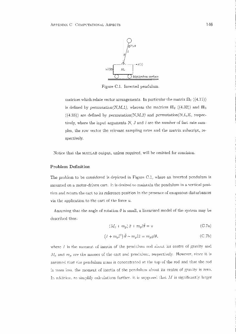
ApPENDIX C COMPUTATIONAL ASPECTS 146
u(t
-x(t)
frictionless surface
Figure C.l. Inverted pendulum.
matrices which relate vector arrangements. In particular the matrix III ((4.11))
is defined by permutation(N,M,l), whereas the matrices II2 ((4.32)) and II3
((4.33)) are defined by permutation(N,M,2) and permutation(N,L,3), respec
tively, where the input arguments N, .J and i are the number of fast rate sam
ples, the row vector the relevant sampling rates and the matrix subscript, re
spectively.
Notice that the MATLAB output, unless required, will be omitted for concision.
Problem Definition
The problem to be considered is depicted in Figure C.I, where an inverted pendulum is
mounted on a motor-driven cart. It is desired to maintain the pendulum in a vertical posi
tion and return the cart to its reference position in the presence of exogenous disturbances
via the application to the cart of the force u,
Assuming that the angle of rotation e is small, a linearised model of the system may be
described thus:
(!'vIc + m p) i: + mpl{j = u
(I + Hlpl2) (j + mpl:i' = 7llpgle ,
(C.7a)
(C.7b)
where I is the moment of inertia of the pendulum rod about its centre of gravity and
Ale and m p are the masses of the cart and pendulum. respectively. However, since it is
assumed that the pendulum mass is concentrated at the top of the rod and that the rod
is mass less. the moment of inertia of the pendulum about its centre of gravity is zero.
In addition. to simplify calculations further. it is supposed that I\[ is significantly larger

ApPENDIX C COMPUTATIONAL ASPECTS 147
than In, whence (M + rn) ;:::; M: Therefore, from equations (C.7a,b), the plant can be
described by the following transfer function model:
(C.8)
where in this example the mass of the cart Me is 0.5 kg and the length of the pendulum is
0.5 m. In the first sampling schedule to be considered, the output signals x(t) and e(t) and
the input signals u( t) are sampled at intervals of T IlYh, T Ilvh and TILl s, respectively,
where T is 0.15 s, and
L I = 1, 1'vh = 2 and 1'vh = 3.
Verifying from equations (4.2a,b) that N is 6, the pulse-transform model of the discretised
plant is
(C.9a)
where
and
b1 = (TIN)2 12Me, b: = - (1 - cosh (TIN )-gll)) IMeg
al =2cosh(TINVi1i).
Evidently, equation (C.9a) can be written as the following left-matrix fraction (see (4.6)):
(C.9b)
and b(z,y') ~ [where0] bl + bl z6 I ]
1 - alz61 + z6 2 -b2 - b2z6
1
The problem of deriving the above left-matrix fraction is computed by the POLYNOMIAL
TOOLBOX conversion command rat21mj, where, if the matrices A and b are named (AplyX)
and (BplyX) , respectively, then the script is:
(BplyX,AplyXj = rat21mj(num,den);
BplyX = inv(diag( diag(AplyX{ O}))) *BplyX:
AplyX = inv(diag(diag(AplyX{O})))*AplyX:
:\otice. that the last two lines of the script have been introduced to ensure that the
condition A;;(O) = L i = L 2..... m.. is satisfied.

ApPENDIX C COMPUTATIONAL ASPECTS
The Polynomial Matrix-Vector Lifted System Representation
148
and
The polynomial lifted system representation, specified by equations (4.34) and (4.35),
can be established through the implementation of the techniques described in section 4.l.
Neglecting the noise model temporarily, the fast-sampled outputs y(O) are related to the
slow-sampled control U(O) thus (see (4.10)):
A(q-1)y(0) = BH(q-1)u(O),
where y'(O) = [Y1(0) YI(-l) ... Y1(-5) Y2(0) Y2(-1) ... Y2(-5) rand U(O) = u(O);
A(q-1) = block diag (16 - 2P~1)(q-1) + p~2\q-1),16 _ a1p~1)(q-1) + p~2)(q-1)),
A -1 _ [ b116 + b1P~1)(q-1)] pA (d)( -1) _ p(1)( -1)and, with B(q) - (1)' l q - 6 q
-b216-b2P6 (q-1)
H(q-1) = p~5)(q-1)W1 = [ 1 ]q-1 W 5 '
where
2b1W5q-1
hq-1 + b1q-2
-2b2W5q-l
-b2q-l b2q-2
Construction of the matrices A (Ahat) and BH (Bhat) can be effected for any sampling
ratio N by the following script, which is based on the commands toeplitz, Wmatrix and
Pmairix outlined previously:
Ahat = toeplitz(AplyX,N);
Hhat = Pmatrix(Lbar-l,N)*Wmatrix(L,N):
Bhat = toeplitz(BplyX,N) *Pmatrix(d*ones{1, m),N) *Hhat;
The designation of the permutation matrix TIl in accordance with the following vectors:
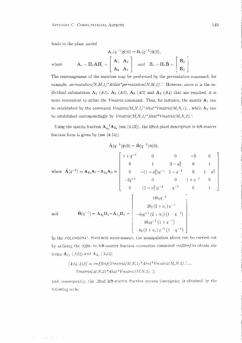
ApPENDIX C COMPUTATIONAL ASPECTS
leads to the plant model
149
Ar(q-I )y(O) = Br(q-I )U(O),
where A e ~ II,AII; ~ [:: .. and Be ~ II,S ~ [ :: ]
The rearrangement of the matrices may be performed by the permutation command; for
example, permutation(N,M,l)*Atilde*permutation(N,M,l). '. However, since it is the in-
dividual submatrices AI (Al), A 2 (A2), A 3 (A3) and A 4 (A4) that are required, it is
more convenient to utilise the Vmatrix command. Thus, for instance, the matrix AI can
be established by the command Vmatrix(M,N,l)*Ahat*Vmatrix(M,N,l). , while A 2 can
be established correspondingly by Vmatrix(M,N,1)*Ahat*Vmatrix(M,N,2). '.
Using the matrix fraction A 42I A 24 (see (4.13)), the lifted plant description in left-matrix
fraction form is given by (see (4.14))
A(q-I)y(O) = B(q-1)u(0),
1 + q-1 0 0 -2 0
0 1 2 - ai 0 1
where - -1-(1 - ai)q-1 1 -I 0 1 - 0.2A(q ) = A42A1-A24A3 = 0 -q 1
') -1 0 0 1 + q-I 0-~q
0 (2 - ai)q-I q-I 0 1
18b1q-I l-2b2 (2 + ad q-l
and - -1B(q ) = A 42B 1-A24B2 = -b2q-1 (2 + ad (1 - q-l)
9b1q-I (1 + q-1)
-b2 (2 + ad q-l (1 + q-l)
In the POLYN01vIIAL TOOLBOX environment, the manipulation above can be carried out
by utilising the right- to left-matrix fraction conversion command rmf2lmf to obtain the
terms A 2 j (A24) and A 42 (A42):
(A24,A42) = rmf2Imf(Vmatrix(AI.N,l) *...J.hat*Vmatrix(AI,N,2). '....
Vmatr'i:r(J1IN,2) *Ahat *Vmatri.T(M,N2). ');
and. consequently, the lifted left-matrix fraction system description is obtained by the
following code:

ApPENDIX C COMPUTATIONAL ASPECTS
Atilde = A42*Vmatrix(M,N,1)*Ahat*Vmatrix(M,N,1). ', ...
A24 *Vmatrix(M,N, 2) *Ahat*Vmatrix(M,N, 1). ';
Btilde = A42*Vmat1'i.r(M,N,l) *Bhat-A24 *Vmatri.r(M,N,2)*Bhat;
Expressed as a right-matrix fraction, the plant model is
150
where inserting the values for the parameters 0,1, b, and b2 , the relevant matrices are given
by
O.0225q-1 O.0328q-2 - O.0328q-3 + O.0225q-4
-O.0467q-1 + O.0467q-2 + O.0467q-3 - O.0467q-4
and Ba(q 1) = -O.0203q-1 - O.0274q-2 + O.l107q-3 - O.0580q-4 - O.0050q-5
O.0056q-1 + O.0199q-2 - O.0717q-3 + O.0199q-4 + O.0056q-5
-O.0050q-1 - O.0580q-2 + O.l107q-3 - O.0274q-4 - O.0203q-5
The equivalent right-matrix fraction description above can be derived directly by the left
to right-matrix fraction conversion command lmj2rmf:
IBa,Ab} = lmj2rmf(Bbar,Abar);
In this example, it is supposed that the disturbance subsystem model is specified by the
matrix
- -1 [1 + C1z61 0 -1]'C(ZN ) =o 1 + c2z6
The procedure summarised in section 4.2 by equations (4.21) and (4.22) can be used to
derive the lifted disturbance subsystem model. The designation of the stable solution
C (Ctilde) can be established through the use of the spectral factorisation command spj
provided within POLYNO;\lIAL TOOLBOX, after the Toepltiz matrix C has been restructured
to establish the matrix r (Gamma). The relevant commands are:
Chat = toeplitz(CplyXN):
Gamma = A42* Vmatri:r(M.N, 1) *Chat-A24 *Vmatrixi M, N,2) *Chat;
Ctilde = spf(Gamma tGamma,1e-10):
Ctilde = inll(diag(diag(Ctilde{ O} ))) -cuu«

ApPENDIX C COMPUTATIONAL ASPECTS 151
It will be observed that the modelling script detailed above has been written in a general
form to enable the code to be extended to any configuration and not limited to the sampling
rates initially selected. In this example, it was found that values Cl and C2 of -0.4313 and
-0.2661 respectively, engenders a C matrix with related zeros very close to the origin.
Consequently, all "C" matrices are henceforth modelled as identity matrices.
LQG Controller Derivation
The representation established above can be used in conjunction with the dynamics
assignment approach to derive the LQG compensator solution for the regulator problem
considered in section 5.1. From the theory detailed in Chapter 5, it is known that the
controller numerator matrix can be defined by
Smd = [8110 8120 8130 8140 0].Inspection of this transposed vector identifies that the concept of causality is not an issue,
and it is therefore possible to employ conventional algorithms to establish the optimal
control solution Rmd (R) and Smd (5) via the diophantine equation defined in equation
((5.25)). The dynamics-assignment approach to determining the LQG controller is de
pendent upon the matrices obtained from the conversions of matrix fraction descriptions
defined in equations (5.2) and (5.24), which can be undertaken by using the macros lmf2rmf
and rmf2lmf as demonstrated above.
The control weighting parameters can be used to move the closed-loop-poles to desirable
location within the unit disc; by trial-and-error, a value of 1 was selected for this example.
Solving equation (5.3) to determine the stable solution d (D) via the spectral factorisation
solver
D = spf(zi*Ab'*Xi*Ab+Ba'*Ba,le-lO):
yields
It will be observed that since the degree of the matrices A b and B; are not equal, an
additional ::;-1 term has been included within the script. thus ensuring that the matrix is
para-Hermitian and that the correct terms are related. The closed-loop poles related to

ApPENDIX C COMPUTATIONAL ASPECTS 152
the plant - determined by the zeros of z4cl(z-1) - are located at z = 0.5124:1:jO.0305 and
z = 0.8754 :1:jO.1101.
The minimal degree solution of the single diophantine equation ((5.25)) is dependent
upon the relevant matrices possessing specific structures. For this reason, in order to
use conventional algorithms, a masking matrix X y (Xy) must be introduced into the
diophantine equations as explained in section C.1. Based upon the structure of the Smd
matrix above, the masking matrix takes the form
X y = diag (1, 1, 1, 1, 0)
Consequently, the minimal degree solution of the single diophantine equation ((5.25)),
defined with respect to R, can be derived from the matrix polynomial equation solver
command xaybc by:
fR,Sj = xaybc(Al,cliag(Xy)Bl,D*Cl, 'miny');
which yields
Rmd = 2.2080+0.3869q-l and Smd = [ -17.1100 16.4029 -119.1203 95.4416 0]
The final stage of the derivation of the optimal matrices R o(q-l) and So(q-l) concerns the
right- to left-matrix fraction conversion of equation (5.5); this procedure is not required
in this example owing to the structure of the C matrices specified above.
Analysis
The performance of the feedback system can be assessed by the response and the margins
of stability of the system, which are given by
GJIu = +15.9317dB and GMl = -6.9511dB.
A simulation of the closed-loop system realised by SI\IULI!'iK produces the responses of
both the outputs and the control signal depicted in Figures C.2 and C.:}.

ApPENDIX C COMPUTATIONAL ASPECTS
EIl'2~I,,:.::2 -0.4Cl _---L__'-----_--'----_---'---_----'-_--'_----'
o I 2 1 4 10
153
f:r=t: -0.1
<-0.2 '
o I 2 3 10
10
Figure C.2. Transient response from an initial pendulum angle.
f:::~ ."~!5..-0.1
'"C5 -02 -"'-----'------'--------"-----o 1 2 3 -\. 10
i'''~'E•...... -0.0)
'-----_--'----_---'---_----"--_--'-__'-----_--'----------.Jo I 2 J
III
Time
Figure ('.:3. Transient response from an initial displacement of the cart.

ApPENDIX C COMPUTATIONAL ASPECTS 154
The values of L 1, lvh and lvh above were chosen primarily for expositional clarity. In a
rather more representative example, it is supposed now that
L I = 4, lvh = 2 and lvf2 = 5,
whence N = 20 (SeE (4.1a,b)).
With the exception of the diophantine equation (5.25) solver, the code defined above
can be used to derive the optimal controller. In this particular situation, the acquisition
of (Ro, So) is dependent upon the use of the masking matrices described in section C.l.
Noting that the last two lines engender the causal structures required, the relevant code
is given by
for i = l:sum(L)
fval(('lr' num2str(i) ',S' num2str(i) 'J -r- .Taybc(diag(Xx(i,:))*Al. '...
'diag(Xy(i,:)) *Bl,D(i,:) *Cl, "miny"); 'J)
eval(f'R(i,l:sum(L)) = r' num2str(i) '*diag(Xx(i,:));'l)
eval(f'S(i,l:sum(M)) = s' num2str(i) '*diag(Xy(i,:));'J)
end
In this case the causal structures of the matrices Smd and R m d are defined by
SIlO 8120 8130 0 8150 0 0
-1 0 0 8240 8250 S260 0Smd =
8211 q
-1 0 0 0 8350 8360 83 7083 1lq
-1 -1 0 0 -1 0 S470S41lq 842lq 845lq
dllo d120 d130 d140
d2 11
q-l i-. d230 d240and R m d =
--0
d3 1l q - 1 d32 1q-l d:330 d340
d4 1l «: d42 l q-1 dB l
q-l d,/.w
therefore, the masking matrices are defined by
XXi = diag (Xr (i. :)). X; =
1
«:' 1
«:' «:'q-l q-l
1 1
1 1
1 1

ApPENDlX C COMPUTATIONAL ASPECTS 155
1 1 1 0 1 1 0
«:' 0 0 1 1 1 0X Yi = diag (Xy(i, :)), X y =
q-l 0 0 0 1 1 1
q-l q-l 0 0 q-l 0 1
Consequently, the optimal control law is defined by:
-9.2692 -89.0946 77.9952 0 8.9156 0 0
9.0924q-l 0 0 -98.4414 -9.4460 86.1802 0So =
8.9156q-l 0 0 0 -9.2692 -95.2219 83.3609
-9.4460q-l 80.6335q-l 0 0 9.0924q-l 0 -92.1074
r 0.8576 0.1030 -0.0125 0
--0.0l28q-l 0.8576 0.2880 0.00044and R o =
l-0.0032Q- , 0 0.8576 0.2489
0.1663q-l -0.0384q-l -0.0128q-l 0.8576
C.4 Conclusion
This section has addressed computational issues associated with the formulation of polyno
mial descriptions and control laws for multirate-sampled systems. In particular, with the
assistance of the computer-aided control system analysis and design package POLYNOMIAL
TOOLBOX to simplify numerical computations and algebraic procedures, an illustrative de
sign example has served to reflect the inherent possibilities of polynomial theory as applied
to multirate systems. Although in some cases the specialised computational techniques
are not directly applicable to the multirate scenario, the simple methods presented III
section C.l can be utilised effectively to overcome such problems.

BIBLIOGRAPHY
Astrom, K J. and Wittenmark, B. (1973). On self-tuning regulators, Automatica 9: 185199.
Astrom, K J. and Wittenmark, B. (1997). Computer Controlled Systems: Theory fj
Design, third edn, Prentice Hall, Englewood Cliffs, NJ.
Al-Rahmani, H. M. and Franklin, G. F. (1990). A new optimal multirate control oflinear periodic and time - invariant systems, IEEE Transactions on Automatic Control35(4): 406-415.
Al-Rahmani, H. M. and Franklin, G. F. (1992). Multirate control: A new approach,Automatica 28(1): 35-44.
Albertos, P., Salt, J. and Tornero, J. (1996). Dual-rate adaptive control, Automatica32(7): 1027-1030.
Amit, N. (1980). Optimal control of multirate digital control systems, Ph.D. dissertation,Department of Aeronautics and Astronautics, Stanford University, Stanford.
Araki, M. (1993). Recent developments in digital control theory, Proceedings of the If!h
Triennial World Congress of the International Federation of Automatic Control, Vol. 9,Sydney, pp. 251-259.
Araki, M. and Hagiwara, T. (1986). Pole assignment by multirate sampled-data outputfeedback, International Journal of Control 44(6): 1661-1673.
Araki, M. and Yamamoto, K (1986). Multivariable multirate sampled-data systems:State-space descriptions, transfer characteristics and nyquist criterion, IEEE Transactions on Automatic Control 31(2): 145-154.
Araki, M., Fukumitsu, K and Hagiwara, T. (1999). Simultaneous stabilization and poleassignment by two level controllers consisting of a gain feedback and a multirate inputcontroller, Journal of Dynamic Systems, Measurement fj Control 121(2): 302-305.
Araki, M., Hagiwara, T. and Soma, H. (1992). Application of multilevel multirate sampleddata controllers to simultaneous pole assignment problem, Proceedings IEEE Conferenceon Decision fj Control, Tucson, pp. 1762-1767.
Arvanitis. K, Kalogeropoulos, G. and Santas, E. (1999). Adaptive pole positioning in?vIlMa linear systems by periodic multirate-input controllers, Journal of MathematicalAnalysis fj Applications 237(2): 463-504.
Arvanitis, K., Paraskevopoules, P. and Vernardos, A. (2000). Multirate adaptive temperature control of greenhouse, Computers and Electronics in Agriculture 26: 30:3-<320.
Bamieh, B .. Pearson, .1., Francis, B. and Tannenbaum (1991). A lifting technique forlinear periodic systems with applications to sampled-data control, Systems and ControlLetters 17: 79-88.
156

BIBLIOGRAPHY 157
Basilio, J. and Kouvaritakis, B. (1997). An algorithm for coprime matrix fraction description using Sylvester matrices, Linear Algebra and its Applications 266: 107-125.
Berg, M. C., Amit, N. and Powell, J. D. (1988). Multirate digital control system design,IEEE Transactions on Automatic Control 33(12): 1139-1150.
Berger, C. and Peduto, D. (1997). Robust digital control using multirate input sampling,International Journal of Control 67(5): 813-824.
Bertsekas, D. (1976). Dynamic Programming and Stochastic Control, Academic Press,New York, USA.
Bittanti, S. and Colaneri, P. (1998). Wiley Encyclopaedia of Electrical and ElectronicEngineering (Ed. J.G. Webster), Vol. 16, Wiley, New York, chapter Periodic control,pp. 59--74.
Bittanti, S., Colaneri, P. and De Nicolao, G. (1988). Two techniques for the solution of thediscrete-time periodic riccati equation, Linear Algebra in Signals, Systems and Controlpp. 3J5-331.
Bittanti, S., Colaneri, P. and De Nicolao, G. (1990). An algebraic ricatti equation for thediscrete-time periodic prediction problem, Systems & Control Letters 14(1): 71-78.
Blankinship, W. A. (1963). A new version of the Euclidean algorithm, American Mathematics monthly 70: 742-745.
Boykin, W. R. and Frazier, B. D. (1975a). Analysis of multi-loop multirate sampled-datasystems, American Institute of Aeronautics and Astronautics Journal 13(4): 453-456.
Boykin, W. H. and Frazier, B. D. (1975b). Multirate sampled-data systems via vectoroperators, IEEE Transactions on Automatic Control 20(4): 548-551.
Carini, P., Micheli, R. and Scattolini, R. (1990). Multirate self-tuning predictive controlwith application to a binary distillation column, International Journal of System Science21(1): 51-64.
Chammas, A. B. and Leondes, C. T. (1979). Pole assignment by piecewise constant outputfeedback, International Journal of Control 29(1): 31-38.
Chen, T. and Qiu, 1. (1994). Roo design of general multirate sampled-data control systems,Automatica 30(7): 1139-1152.
Clarke, D. and Gawthrop, P. (1975). Self-tuning controller, Proceedings of the Institute ofElectT'ical and Electronic Engineering 122: 9299:l!.
Clarke. D., Mohtadi, C. and Tuffs, P. (1987:1). Generalized predictive control _.. Pt. 1: Thebasic algorithm, Automatica 23(2): 137-148.
Clarke. D., Moht.adi, C. and Tuffs, P. (1987b). Generalized predictive control - Pt. 2:Extensions and interpretations, A utomatica 23(2): 149--160.

BIBLIOGRAPHY 158
Coffey, T. and Williams, I. (1966). Stability analysis of rnultiloop, multirate sampledsystems, American Institute of Aeronautics and Astronautics Journal 4(12): 2178~2190.
Colaneri, P. and De Nicolao, G. (1995). Multirate LQG control of continuous-time stochastic systems, Automatica 31(4): 591-596.
Colaneri, P., Scattolini, R. and Schiavoni, N. (1992). LQG optimal control of multiratesampled-data systems, IEEE Transactions on Automatic Control 37(5): 675-682.
Cutler, C. and Ramaker, B. (1979). Constrained multivariable control of a hydrocrackerreactor, Proc. Am. Control Conference, pp. 1014-1020.
Datta, K. and Gangopadhyay, S. (1992). Coprime matrix fraction description via orthogonal structure theorem, IEEE Transactions on Automatic Control 37: 1517-1520.
De Keyser, R. and Van Cauwenberghe, A. (1982). Typical application possibilities forself-tuning predictive control, Proceedings IFA C Symp. on Identification fj System Parameter Estimation, Vol. 2, pp. 1552-1557.
Er, M. J. and Anderson, B. D. (1991). Practical issues in multirate output controllers,International Journal of Control 53(5): 1005-1020.
Er, M. J. and Anderson, B. D. (1992). Performance study of multirate output controllersunder noise disturbances, International Journal of Control 56(3): 531-545.
Er, M. J., Anderson, B. D. and Yan, W.-Y. (1994). Gain margin improvements using generalized sampled-data hold function based multirate output compensators, A utomatica30(3): 461-470.
Gantmakher, F. (1959). The Theory of Matrices, Vol. 1 and 2, Chelsea Publishing, NewYork.
Garcia, C., Prett, D. and Morari, M. (1991). Model predictive control: theory and practice- a survey, Automatica 25: 335-348.
Glasson, D. P. (1983). Development and applications of multirate digital control, IEEEControl Systems Magazine 3(4): 2-8.
Godbout, L. F., Jordan, D. and Striefler, M. E. (1994). Pole placement algorithms formultirate-sampled linear systems, Automatica 30(4): 723-727.
Guilandoust, M., Morris, A. and Tham, M. (1987). Adaptive inferential control, Proceedings of the Institution of Electrical Engineers, part D 134: 171-179.
Hagiwara, T and Araki, M. (1988). Design of a stable state feedback controller based onthe multirate sampling of the plant output, IEEE Transactions on Automatic Control33(9): 812-819.
Hagiwara, T, Fujimura, T and Araki, ;vI. (1990). Generalized multirate-output controllers, Iniernational Journal of Control 52(:3): 597-612.
Horowitz, 1. (196:3). Synthesis of Feedback Systems. Academic: Press. New York.

BIBLIOGRAPHY 159
Hunt, K. and Sebek, M. (1989). Optimal multivariable regulation with disturbance measurement feedforward, International Journal of Control 49: 373378.
Jezek, J. (1982). New algorithm for minimal solution of linear polynomial equations,Kybernetika 18(6): 505-516.
Jezek, J. and Kucera, V. (1985). Efficient algorithm for matrix spectral factorisation,Automatica 21(6): 663-669.
Jury, E. 1. (1961). Sampling schemes in sampled-data control systems, IRE Transactionson Automatic Control pp. 86-88.
Jury, E. 1. (1967). A note on multirate sampled-data systems, IEEE Transactions onAutomatic Control 12: 319-320.
Kabarnba, P. (1987). Control of linear systems using generalised sampled-data hold functions, IEEE Transactions on Automatic Control 32: 772-783.
Kaczorek, T. (1985). Pole-placement for linear discrete-time systems by periodic outputfeedbacks, Systems and Control Letters (6): 267-269.
Kalman, R. and Bertram, J. (1959). A unified approach to the theory of sampling systems,Journal of the Franklin Institute 267: 405-436.
Kando, H. and Iwazumi, T. (1986). Multirate digital control design of an optimal regulatorvia singular perturbation theory, International Journal of Control 44(6): 1555-1578.
Krane, G. (1957). Input-output analysis of multirate feedback systems, IRE Transactionson Automatic Control 3: 21-28.
Kucera, V. (1979). Discrete Linear Control - The polynomial equation approach, Wiley,Chichester, UK.
Kucera, V. (1991). Analysis and Design of Discrete Linear Control Systems, Prentice Hall,Hemel Hempstead, UK.
Kucera, V. (1993). Diophantine equations in control - a survey, Automatica 29(6): 13611375.
Kucera, V. and Sebek, M. (1984). A polynomial solution to regulation and tracking, Pt.1, Kybernetika 20: 177-188.
Kwakernaak, H. (2000). A descriptor algorithm for the spectral factorisation of polynomialmatrices, IFAC Symposium on Robust Control Design, Prague, Czech Republic.
Kwakernaak. H. and Sebek, xr. (1994). Polynomial j-spectral factorization, IEEE Transactions on Automatic Control 39(2): 315-328.
Kwakcrnaak, H. and Sebek. :\1. (1999). Polynomial Toolbox 2.0 Manual, The Polyx.

BIBLIOGRAPHY 160
Lee, J., Gelormino, M. S. and Morari, M. (1992). Model predictive control of multirate sampled data systems: a state-space approach, International Journal of Control55(1): 153-191.
Lee, J.-W. and Oh, J .-H. (2000). Comparison of performance and computational efficiencyin rnultirate LQG control, International Journal of Systems Science 31(5): 669-676.
Lennartson, B. (1988). Periodic solutions of riccati equations applied to multirate sampling, International Journal of Control 48(3): 1025-1042.
Ling, K. and Lim, K. (1996). A state-space GPC with extensions to multirate control,Automatica 32(7): 1067-1071.
Liu, G. and Patton, R. (1998). Multirate sampled-data system control via eigenstructureassignment, Eigenstructure assignment for control system design, Wiley, Chichester,chapter 8.
Longhi, S. (1994). Structural properties of rnultirate sampled-data systems, IEEE Transactions on Automatic Control 39(3): 692-696.
Lu, W., Fisher, D. G. and Shah, S. L. (1990). Multirate constrained adaptive control,International Journal of Control 51(6): 1439-1456.
MacFarlane, A. G. and Postlethwaite, 1. (1977). The generalised nyquist stability criterionand multivariable root loci, International Journal of Control 25: 81-127.
Mahmood, S., Pugh, A., Karampetakis, N. and Hayton, G. (1998). Structural propertiesof column (row) reduced MFDs, International Journal of Control 69(1): 111-130.
Meyer, D. G. (1990a). A new class of shift-varying operators, their shift-invariantequivalents and multirate digital systems, IEEE Transactions on A utomatic Control35(4): 429-433.
Meyer, D. G. (1990b). A pararneterisation of stabilizing controllers for multirate sampleddata systems, IEEE Transactions on Automatic Control 35(2): 233-236.
Meyer, D. G. (1992). Cost translation and a lifting approach to the multirate LQGproblem, IEEE Transactions on Automatic Control 37(9): 1411--1415.
Meyer, D. G. and Burrus, C. (1975). A unified analysis of multirate and periodicallytime-varying digital filters, IEEE Transactions on Circuit and Systems 22: 16.5-168.
Xloore, K. 1., Bhatt.acharvya, S. and Dahleh, :\1. (1993). Capabilities and limitations ofmultirate control schemes. Automatica 29(4): 941951.
:\"ewton, G., Gould, 1. and Kaiser, J. (1957). Analytical Design of Linear Feedback Controls, Wiley, New York.
Patel. R. (1981). Computation of matrix fraction descriptions of linear time-invariantsvst cms. IEEE Transactions on Auiomaiic Control 26: 148-161.

BIBLIOGRAPHY 161
Peterka, v. (1972). On steady state mmimum variance control strategy, Kybernetika8: 219-232.
Peterka, V. (1984). Predictor-based self-tuning control, Automatica 20: 39-50.
Prett, D. and Gillette, R (1979). Optimisation and constrained multivariable control ofa catalytic cracking unit, AIChE National Mtg, Houston, Texas.
Qiu, L. and Chen, T. (1994). H 2-opt imal design of multirate sampled-data systems, IEEETransactions on Automatic Control 39(12): 2506-2511.
Ragazzini, .1. and Franklin, G. F. (1958). Sampled Data Control Systems, McGraw Hill,New York.
Ravi, R, Khargonekar, P., Minto, K. and Nett, C. (1990). Controller parameterisationfor fast-rate time-varying multirate plants, IEEE Transactions on A utomatic Control35(11): 1259-1262.
Richalet, .1., Rault, A.) Testud, .1. and Papon, .1. (1978). Model predictive heuristic control,Automatica 14: 413-428.
Rosenbrock, H. (1970). State space and multivariable theory, Wiley-lnterscience, NewYork.
Sagfors, M. F., Toivorien, H. and Lennartson, B. (2000). State-space solution to theperiodic multirate H oo control of multirate: A lifting approach, IEEE Transactions onAutomatic Control 45(12): 2345-2350.
Sain, M. (1975). A free-modular algorithm for minimal design of linear multivariablesystems, Proceedings of the 6th IFAC Congress, Boston.
Scattolini, R (1988). Self-tuning control of systems with infrequent and delay outputsampling, Proceedings of the Institution of Electrical Engineers, part D 35: 213-221.
Scattolini, R. and Schiavoni, N. (1995). A multirate model-based predictive controller,IEEE Transactions on Automatic Control 40(6): 1093-1097.
Schauer, T. and Hunt, K. (2000). Linear modelling and controller design for the singlelimb movement of paraplegics using FES, Proceedings of the 4th IFAC Symposium onModelling and Control in Biomedical Systems, Greifswald, Germany.
Sebek, M. (1981). Optimal tracking via polynomial matrix equations, International Journal of Systems Science 12: 357-369.
Sebek, :vI. (1983). Direct polynomial approach to discrete-time stochastic tracking. Problems of Control and Information Theory 12: 29:3-:302.
Sebek. Xl. (1993). Polynomial methods in optimal control and filtering, lEE Control Engineering Series, Peter Peregrinus, London. chapter 10: .I-Spectral factorisation algorithms.

BIBLIOGRAPHY 162
Sebek, M. and Kucera, V. (1981). Matrix equations arising in regulator problems, Kybernetika 17: 128-139.
Sebek, M. and Kucera, V. (1982). Polynomial approach to quadratic tracking in discretelinear systems, IEEE Transactions on A utomatic Control 27: 1248-1250.
Sebek, M., Kwakcrnaak, H., Hcnrion, D. and Pejchova, S. (1998). Recent progress inpolynomial methods and polynomial toolbox for MATLAB version 2.0, Proceedings of theConference on Decision and Control, IEEE, Tampa, Florida, pp. 3661-3668.
Shu, H. and Chen, T. (1995). State-space approach to discrete-time H 2-optimal controlwith a causality constraint, Systems B Control Letters 26(1): 69-77.
Sklansky, J. and Ragazzini, J. (1955). Analysis of errors in sampled-data feedback systems,AlEE Transactions 74: 65-71.
Soderstrom, T. (1980). Methods and applications in adaptive control, Berlin, SpringerVerlag.
Sternad, M. and Ahlen, A. (1993). A novel derivation methodology for polynomial - LQcontroller design, IEEE Transactions on Automatic Control 38(1): 116-121.
Strijbos, R. (1996). Calculation of right matrix fraction descriptions: an algorithm, Proceedings of the 4th IEEE Mediterranean Symposium on New Directions in Control andAutomation, Maleme, Krete, Greece, pp. 478-482.
Thompson, P. (1986). Gain and phase margins of multirate sampled-data feedback systems, International Journal of Control 44(3): 833-846.
Truman, A. W. and Govan, M. (2000a). Multirate-sampled digital feedback system designvia a predictive control approach, lEE Proceedings - Control Theory B Applications147(3): 293-302.
Truman, A. W. and Govan, M. (2000b). Polynomial LQG design of subrate digital feedbacksystems via frequency decomposition, Optimal Control Applications BMethods 21: 211232.
Truman, A. W. and Govan, M. (2000c). Polynomial LQG synthesis of subrate digitalfeedback systems, lEE Proceedings - Control Theory [3 Applications 147(3): 247-256.
Truman, A. W. and Govan, M. (2001). Predictive control of fast output-sampled digitalfeedback systems via a polynomial approach, Proceedings of the Institution of Mechanical Engineers, part 1215: 211--233.
Tuel, \V. J. (1968). Computer algorithm for spectral factorisation of rational matrices,IBM Journal Research Development 12: 163-170.
Viassolo, D. E. and Rotea, :'1. A. (1998). Practical design of multirate output controllers,Proceedings of the 37th IEEE Conference on Decision f1 Control. Tampa, USA, pp. :3373~2.

BIBLIOGRAPHY
Volgin, L. (1962). The elements of the theory of controllers, Soviet Radio, Moscow.
163
Voulgaris, P. G. and Bamieh, B. (1993). Optimal Hex; and H 2 control of hybrid multiratesystems, Systems 8 Control Letters 20(4): 249~261.
Voulgaris, P. G., Dahleh, M. A. and Valavani, L. S. (1994). u.; and H2 optimal controllersfor periodic and rnultirate systems, A uiomatica 30(2): 251--263.
Werner, H. (1998). Multimodel robust control by fast output sampling - an LMI approach,Automatica 34(12): 1625-1630.
Werner, H. (1999). Tracking and disturbance rejection for an uncertain system using fastoutput sampling, European Journal of Control 5(1): 129-137.
Wiener, N. (1949). Extrapolation, Interpolation and Smoothing of Stationery Time Series,Wiley, New York.
Wolovich, W. (1974). Linear Muliioarioble Systems, Springer, New York.
Ydstie, B. (1984). Extended horizon adaptive control, 9th World Congress of the IFAC,Budapest, Hungary.
Yen, N.-Z. and Wu, Y-C. (1993). On a general optimal algorithm for multirate output feedback controllers for linear stochastic periodic systems, IEEE Transactions onAutomatic Control 38(6): 939-943.
Youla, D. C., Bongiorno, J. J. and Jabr, H. A. (1976a). Modern Wiener-Hopf designof optimal controllers - Pt. 1: the single-input-output case, IEEE Transactions onAutomatic Control 21(1): 3-13.
Youla, D. C., Jabr, H. A. and Bongiorno, J. J. (1976b). Modern Wiener-Hopf design ofoptimal controllers -- Pt. 2: the multivariable case, IEEE Transactions on AutomaticControl 21(3): 319-338.
Zhang, Q. and Tomizuka, M. (1988). Multirate sampling adaptive control and its application to thermal systems, International Journal of Control 47: 135-144.


![Multirate Sampled-Data Systems: All H/spl infin/ Suboptimal … · troller design, e.g., stabilizing controller design and parameter-ization of all stabilizing controllers [11], [30],](https://img.dokumen.tips/doc/110x75/5af8450f7f8b9ad2208c5710/multirate-sampled-data-systems-all-hspl-infin-suboptimal-design-eg-stabilizing.jpg)