Embed Size (px)
DESCRIPTION
Contains few slides and notes describing multirate signal processing. Its good for beginners
Citation preview
Module 5 - Multirate Signal Processing
Patrick A. Naylor
Digital Signal Processing – p.1/25
Contents
Applications of multirate signal processing
Fundamentalsdecimationinterpolation
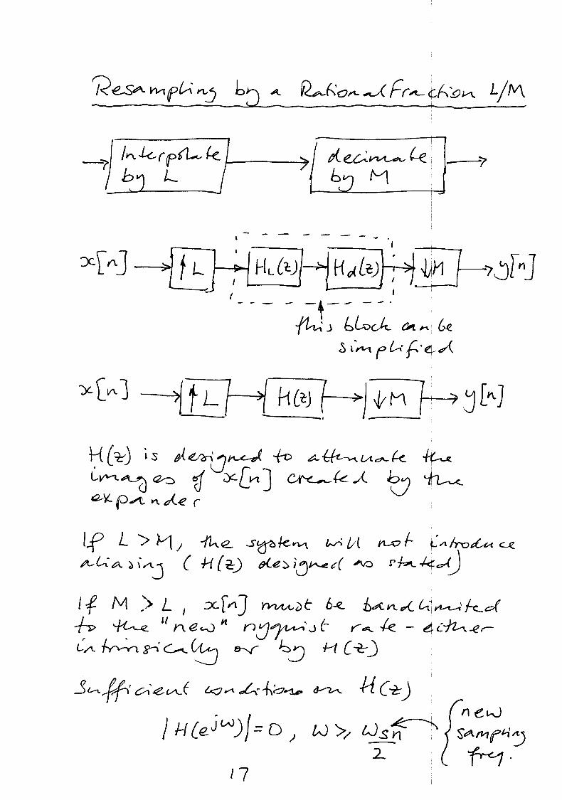
Resampling by rational fractions
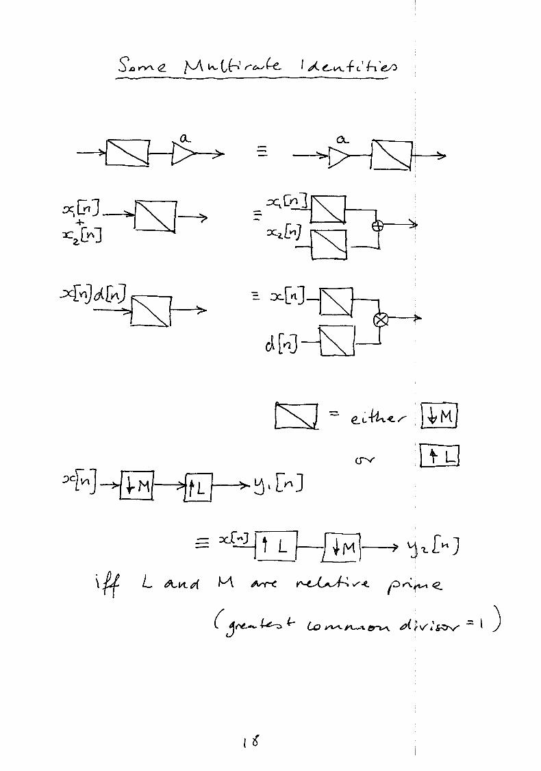
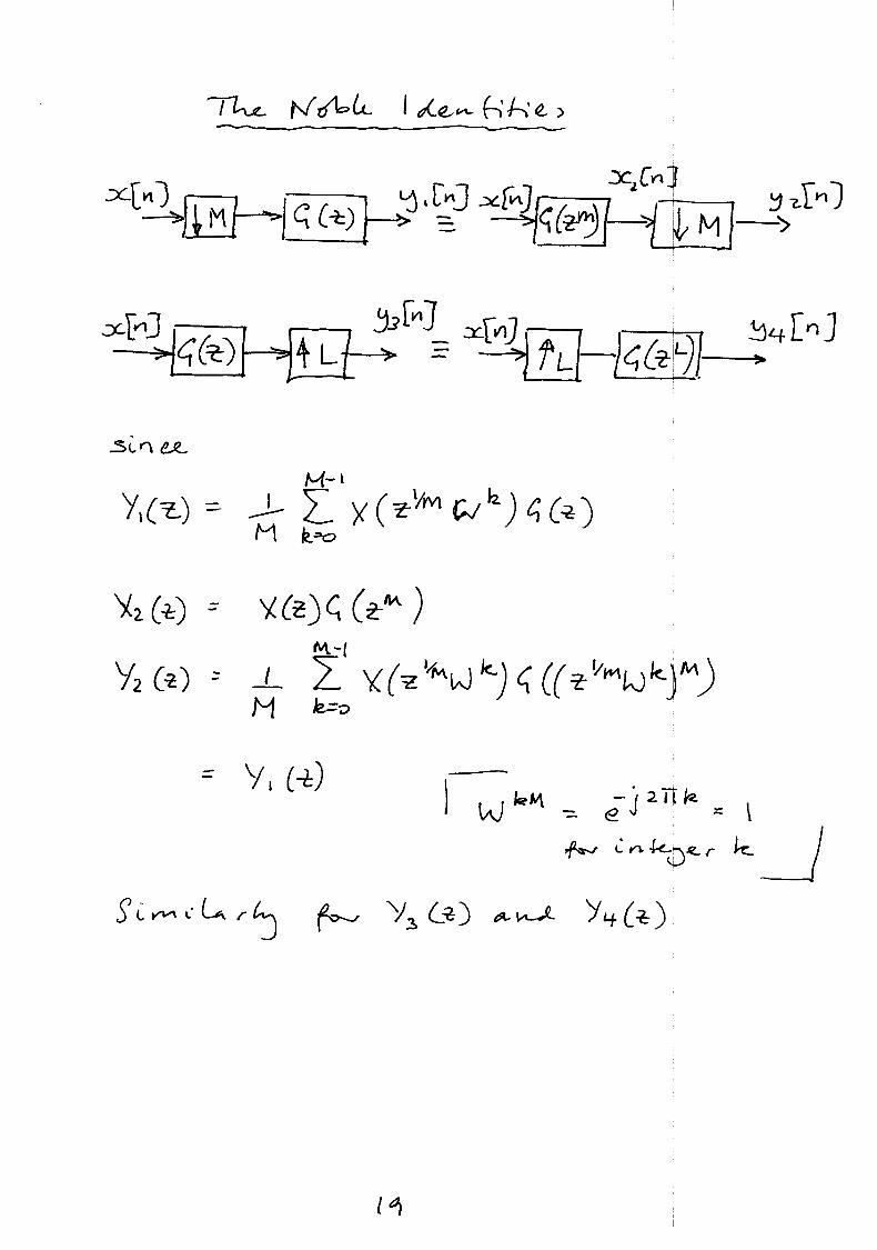
Multirate identities
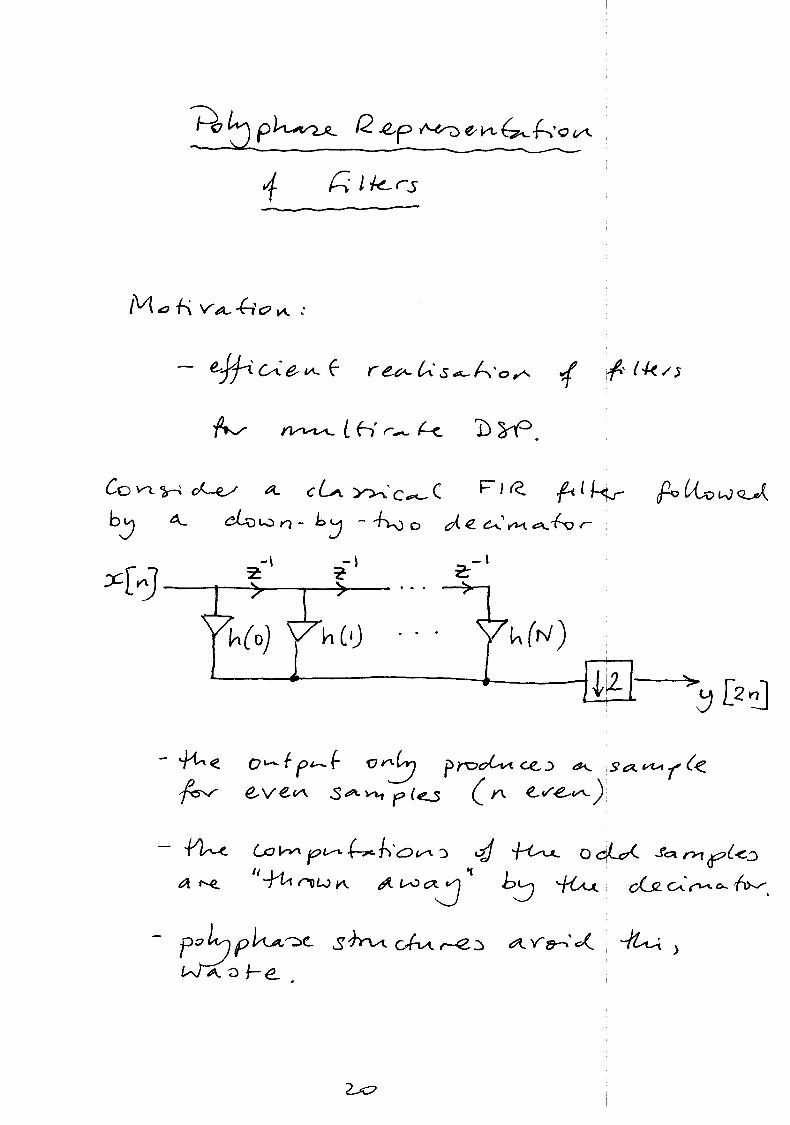
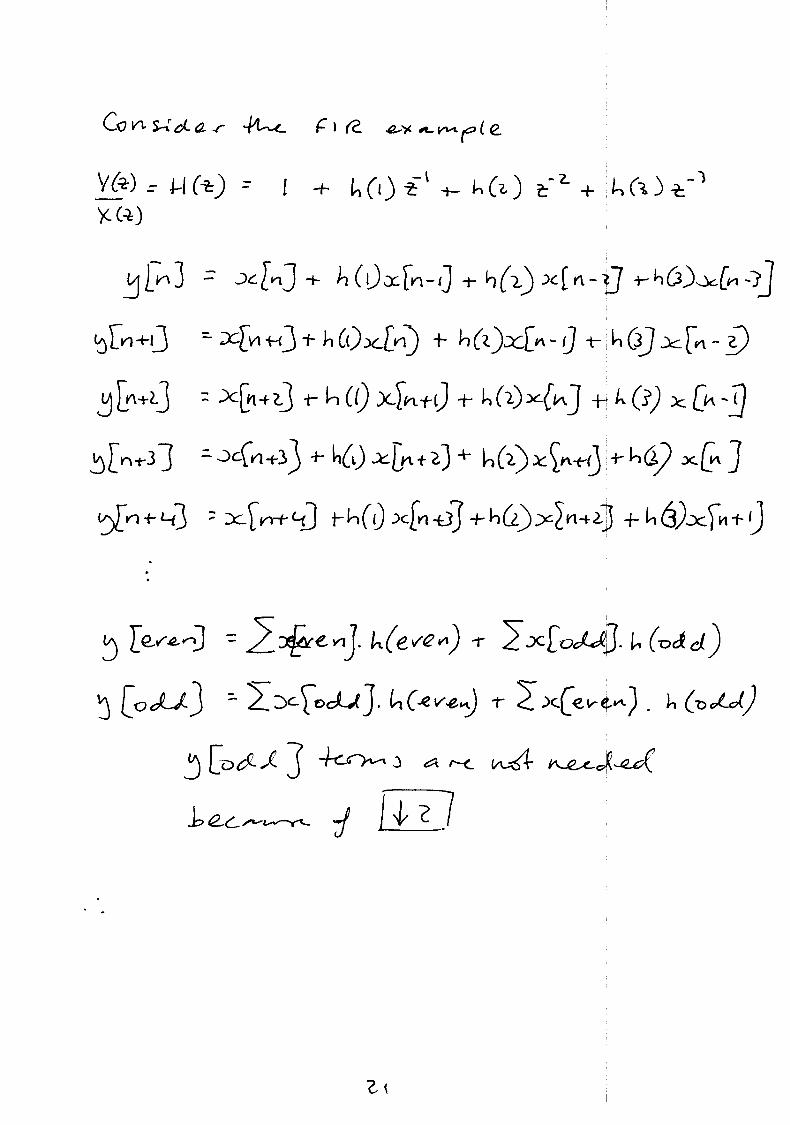
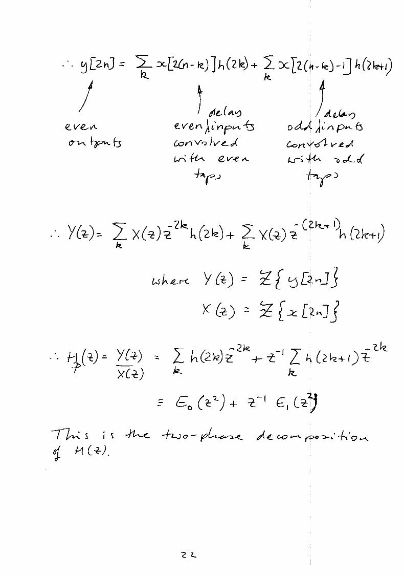
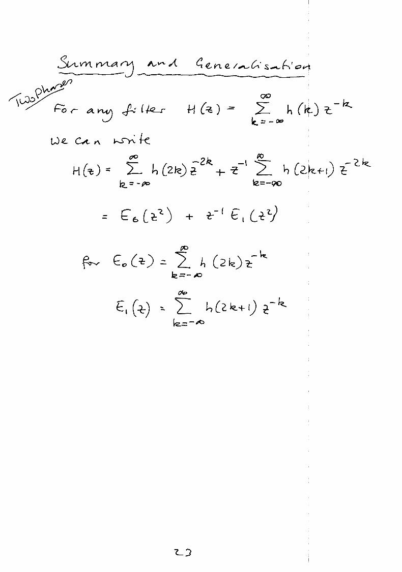
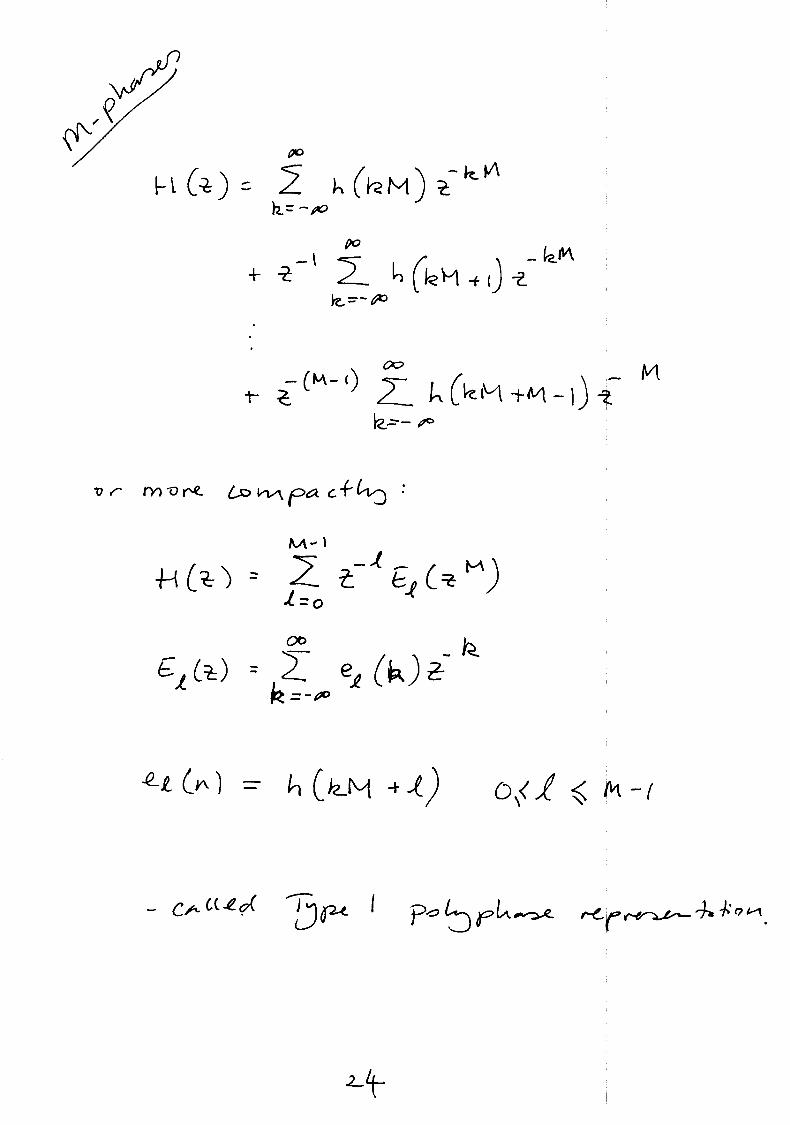
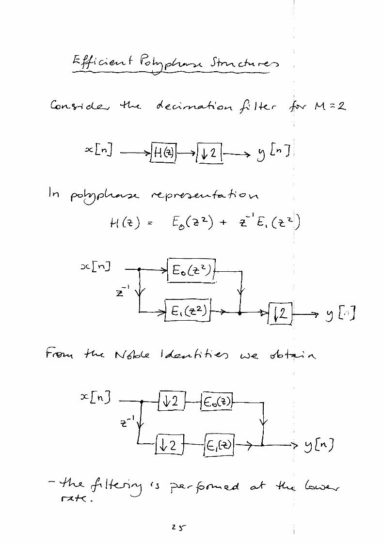
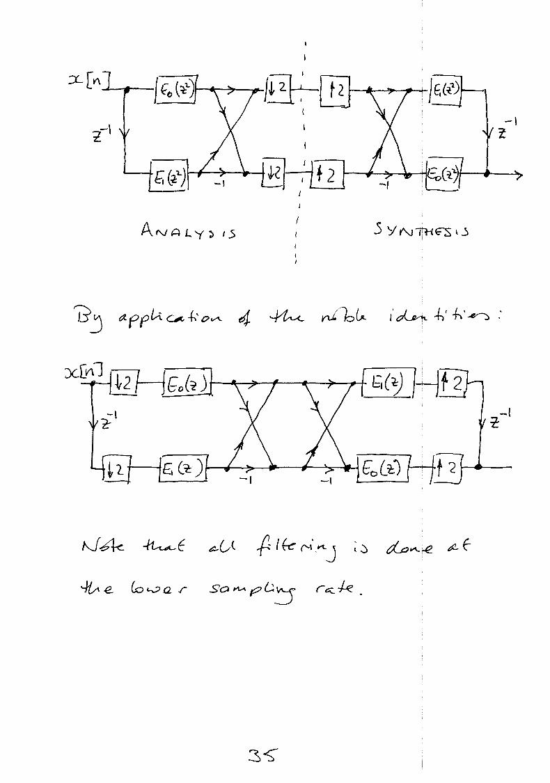
Polyphase representations
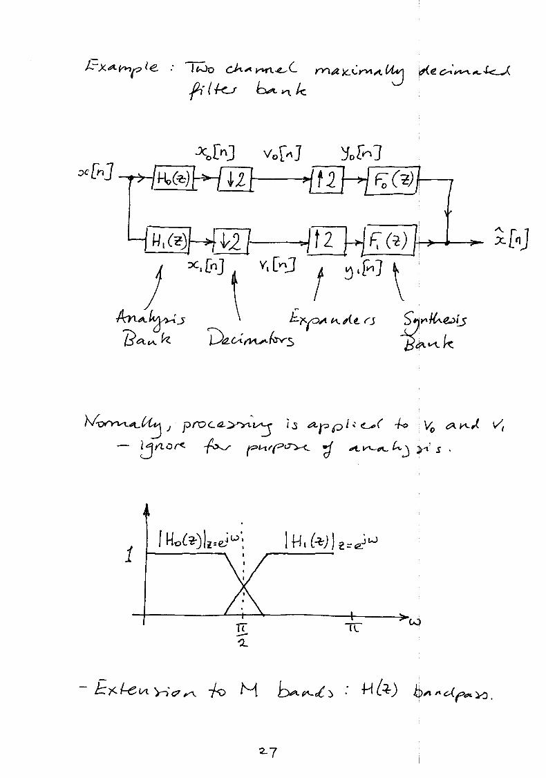
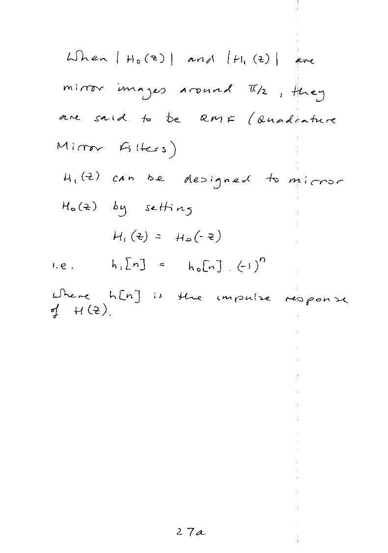
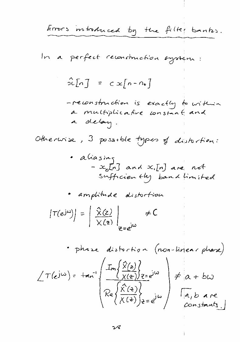
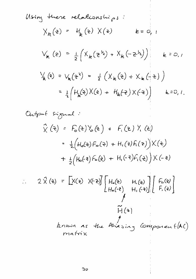
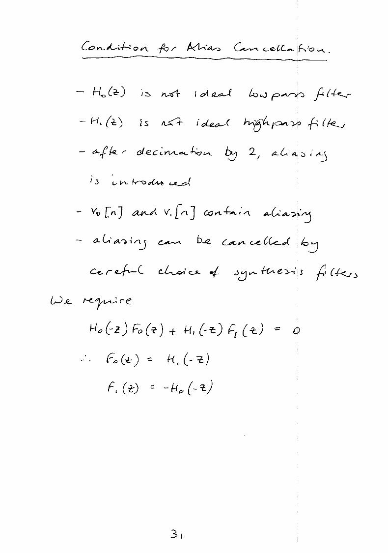
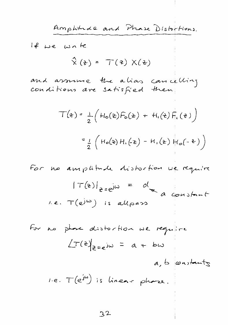
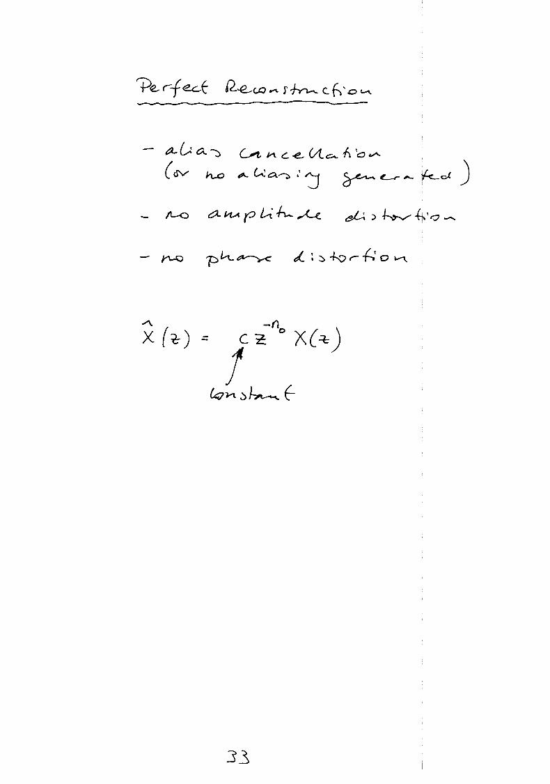
Maximally decimated filter banksaliasingamplitude and phase distortionperfect reconstruction conditions
Digital Signal Processing – p.2/25
Introduction
In single-rate DSP systems, all data is sampled at the same rateno change of rate within the system.
In multirate DSP systems, sample rates are changed (or are different)within the system
Multirate can offer several advantagesreduced computational complexityreduced transmission data rate.
Digital Signal Processing – p.3/25
Example: Audio sample rate conversion
recording studios use 192 kHzCD uses 44.1 kHzwideband speech coding using 16 kHz
master from studio must be rate-converted by a factor
44.1
192
Digital Signal Processing – p.4/25
Example: Oversampling ADC
Consider a Nyquist rate ADC in which the signal is sampled at the desiredprecision and at a rate such that Nyquist’s sampling criterion is justsatisfied.
Bandwidth for audio is 20 Hz < f < 20 kHz
Antialiasing filter required has very demanding specification
|H(jω)| = 0 dB, f < 20 kHz
|H(jω)| < 96 dB, f ≥44.1
2kHz
Requires high order analogue filter such as elliptic filters that have verynonlinear phase characteristics
hard to design, expensive and bad for audio quality.
Digital Signal Processing – p.5/25
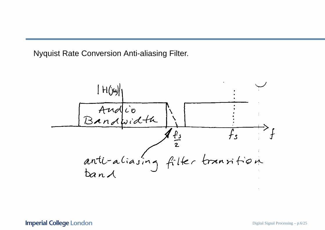
Nyquist Rate Conversion Anti-aliasing Filter.
Digital Signal Processing – p.6/25
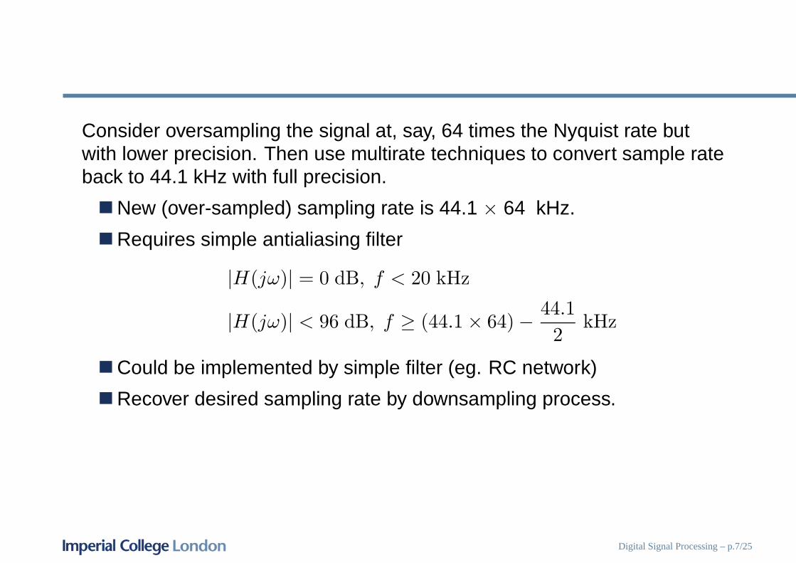
Consider oversampling the signal at, say, 64 times the Nyquist rate butwith lower precision. Then use multirate techniques to convert sample rateback to 44.1 kHz with full precision.
New (over-sampled) sampling rate is 44.1 × 64 kHz.
Requires simple antialiasing filter
|H(jω)| = 0 dB, f < 20 kHz
|H(jω)| < 96 dB, f ≥ (44.1 × 64) −44.1
2kHz
Could be implemented by simple filter (eg. RC network)
Recover desired sampling rate by downsampling process.
Digital Signal Processing – p.7/25
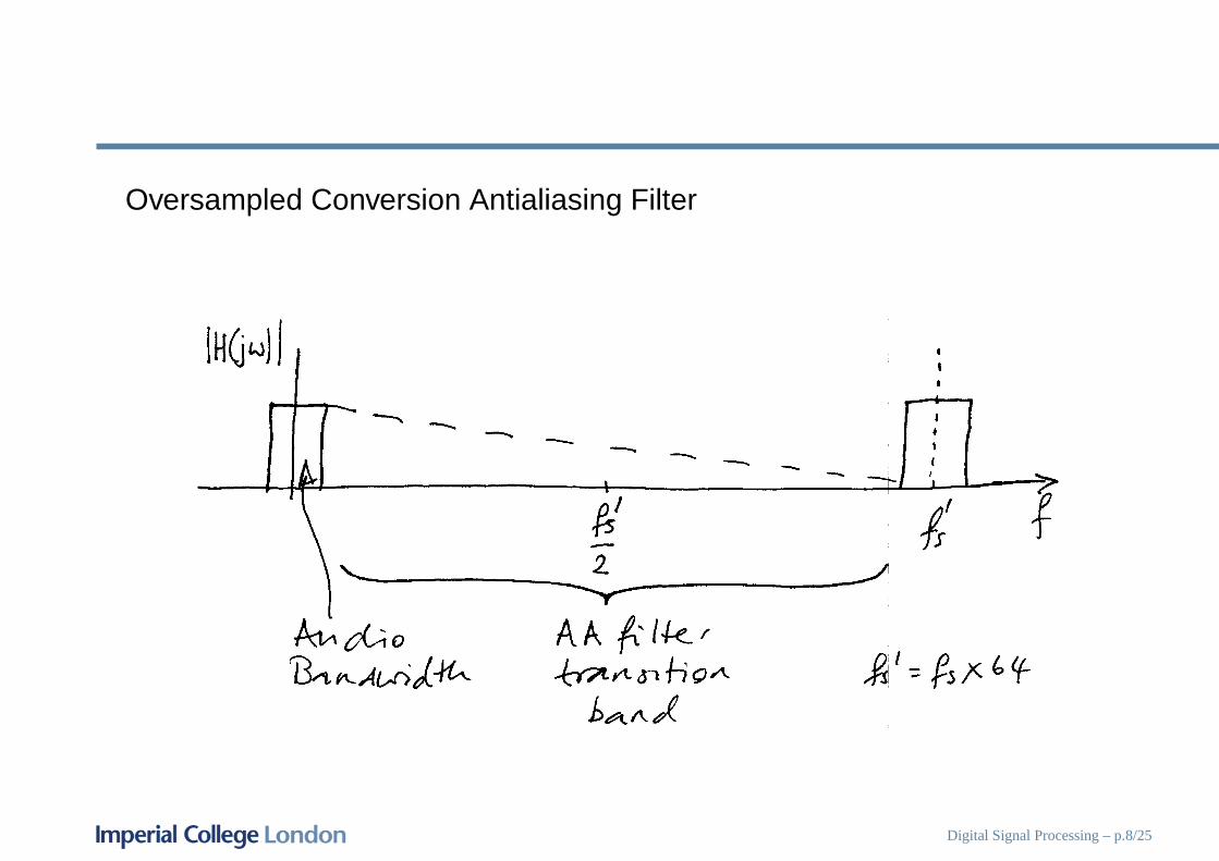
Oversampled Conversion Antialiasing Filter
Digital Signal Processing – p.8/25
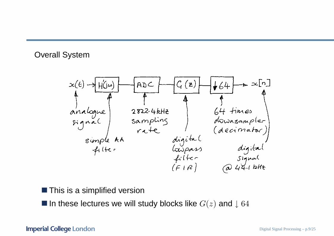
Overall System
This is a simplified version
In these lectures we will study blocks like G(z) and ↓ 64
Digital Signal Processing – p.9/25
Example: Subband Coding
Consider quantizing the samples of a speech signal. How many bits arerequired?
In general, 16 bits precision per sample is normally used for audio.This gives an adequate dynamic range.
In practice, certain frequency bands are less important perceptuallybecause they contain less significant information
bands with less information or lower perceptual importance may bequantized with lower precision - fewer bits.
Divide the spectrum of the signal into several subbands then allocatebits to each band appropriately.
Digital Signal Processing – p.10/25
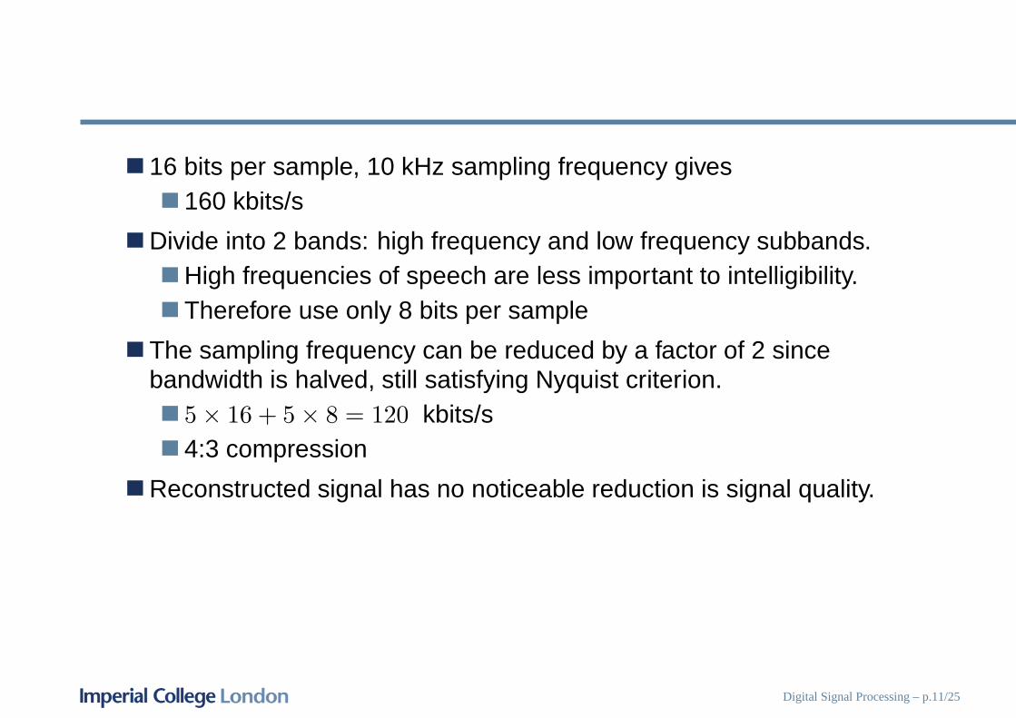
16 bits per sample, 10 kHz sampling frequency gives160 kbits/s
Divide into 2 bands: high frequency and low frequency subbands.High frequencies of speech are less important to intelligibility.Therefore use only 8 bits per sample
The sampling frequency can be reduced by a factor of 2 sincebandwidth is halved, still satisfying Nyquist criterion.
5 × 16 + 5 × 8 = 120 kbits/s4:3 compression
Reconstructed signal has no noticeable reduction is signal quality.
Digital Signal Processing – p.11/25
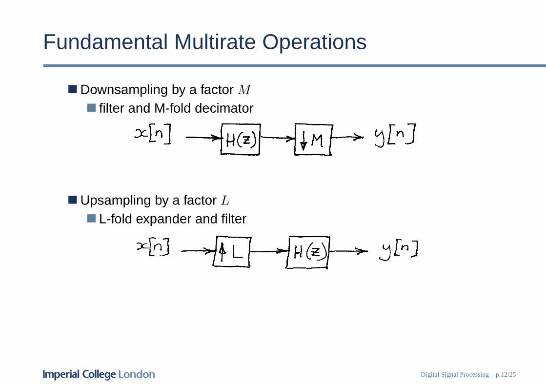
Fundamental Multirate Operations
Downsampling by a factor M
filter and M-fold decimator
Upsampling by a factor L
L-fold expander and filter
Digital Signal Processing – p.12/25
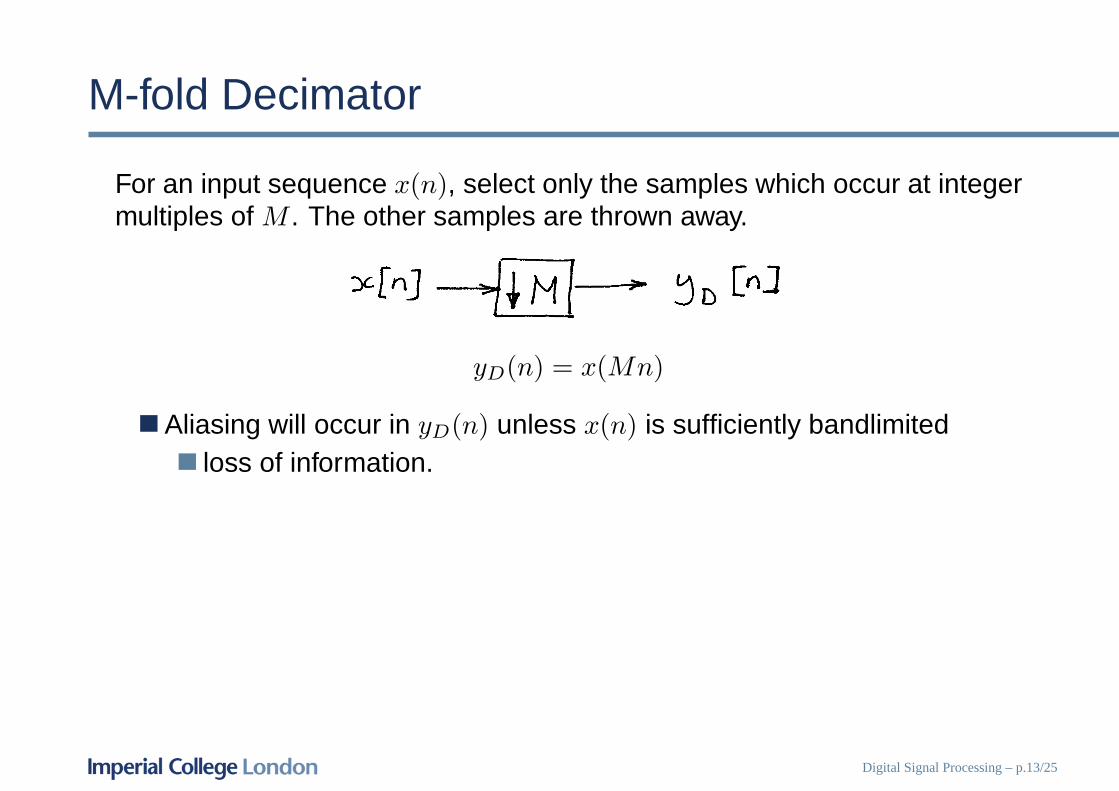
M-fold Decimator
For an input sequence x(n), select only the samples which occur at integermultiples of M . The other samples are thrown away.
yD(n) = x(Mn)
Aliasing will occur in yD(n) unless x(n) is sufficiently bandlimitedloss of information.
Digital Signal Processing – p.13/25
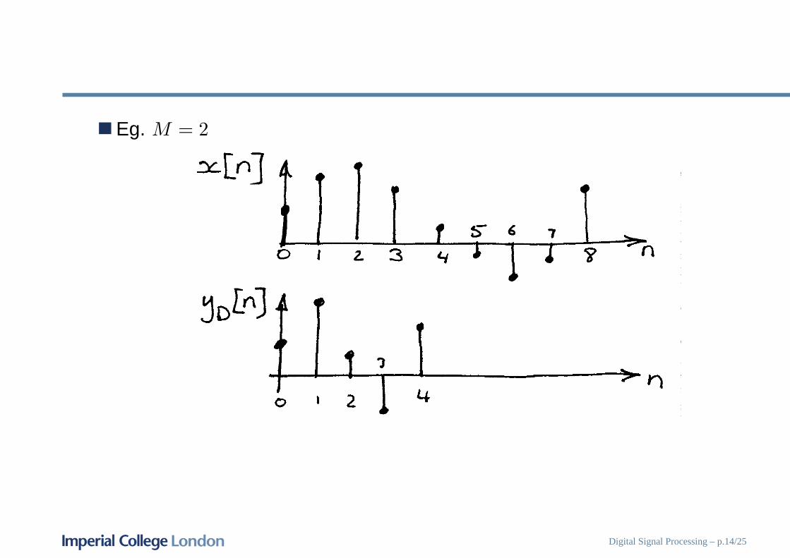
Eg. M = 2
Digital Signal Processing – p.14/25
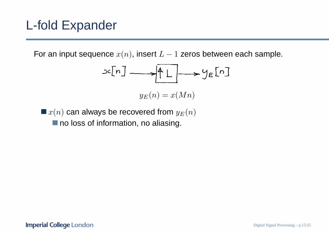
L-fold Expander
For an input sequence x(n), insert L − 1 zeros between each sample.
yE(n) = x(Mn)
x(n) can always be recovered from yE(n)
no loss of information, no aliasing.
Digital Signal Processing – p.15/25
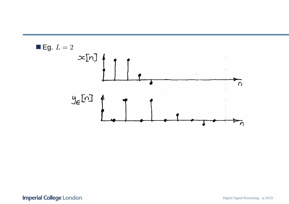
Eg. L = 2
Digital Signal Processing – p.16/25
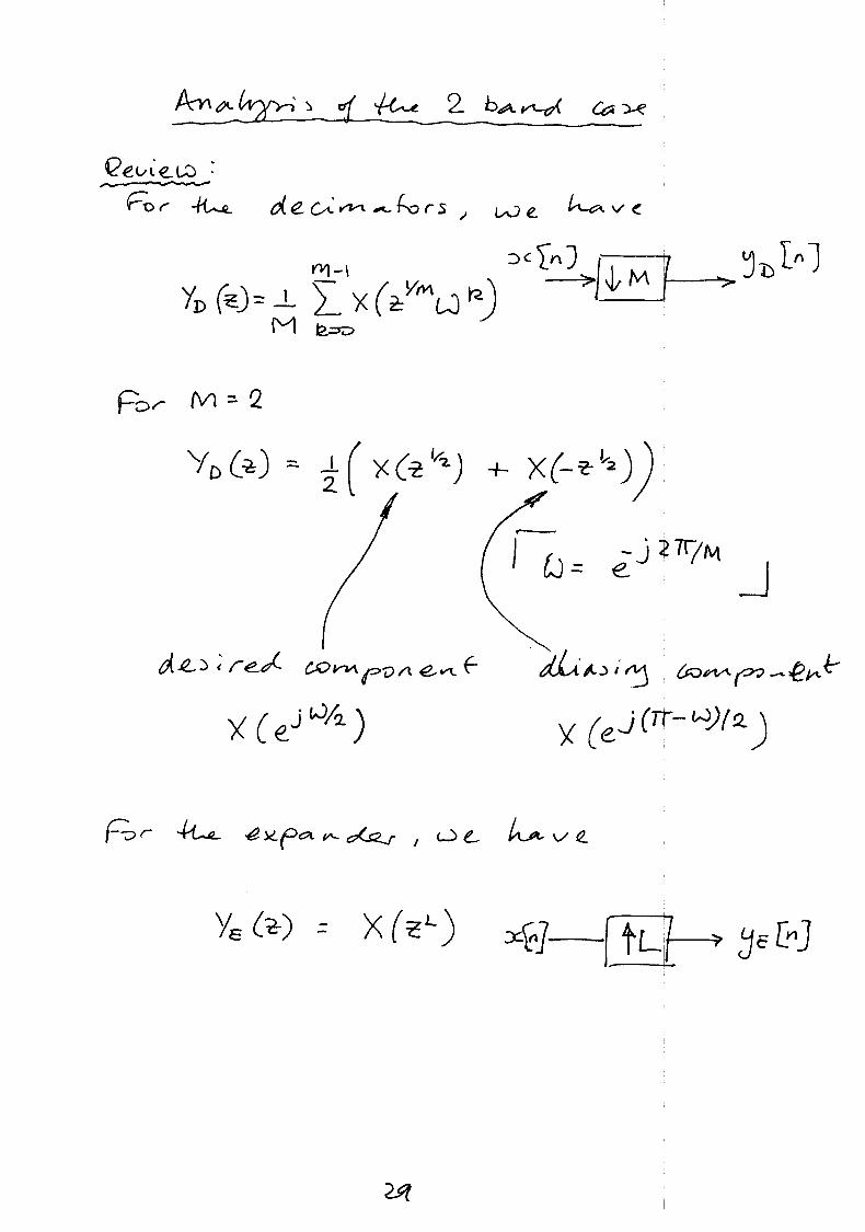
Frequency Domain View of the Expander
From the definition of the z-transform
YE(z) =
∞∑
n=−∞
yE(n)z−n
=∞∑
k=−∞
yE(kL)z−kL
=
∞∑
k=−∞
x(k)z−kL = X(zL)
For frequency response write z = ejω giving
YE(ejω) = X(ejωL)
YE is a compressed version of X
Multiple images of X(ejω) are created in YE(ejω) between ω = 0 andω = 2π
Digital Signal Processing – p.17/25
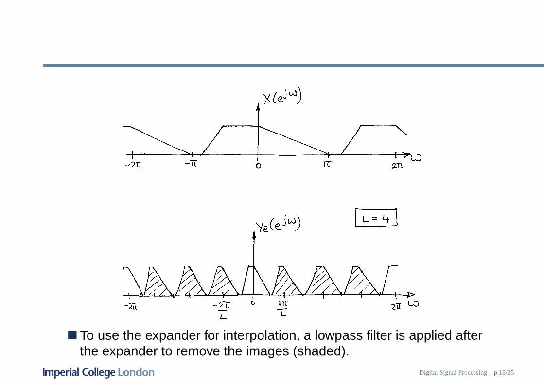
To use the expander for interpolation, a lowpass filter is applied afterthe expander to remove the images (shaded).
Digital Signal Processing – p.18/25
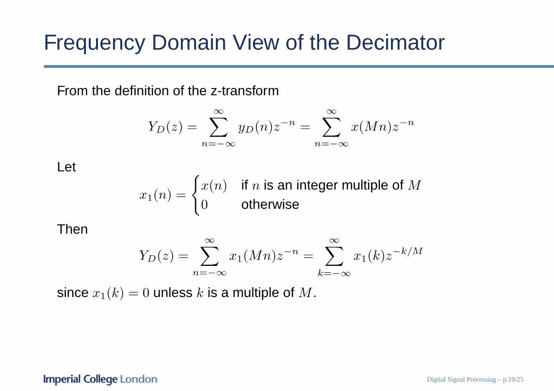
Frequency Domain View of the Decimator
From the definition of the z-transform
YD(z) =
∞∑
n=−∞
yD(n)z−n =
∞∑
n=−∞
x(Mn)z−n
Let
x1(n) =
{
x(n) if n is an integer multiple of M
0 otherwise
Then
YD(z) =∞∑
n=−∞
x1(Mn)z−n =∞∑
k=−∞
x1(k)z−k/M
since x1(k) = 0 unless k is a multiple of M .
Digital Signal Processing – p.19/25
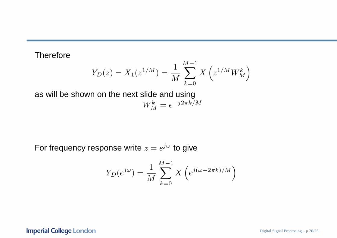
Therefore
YD(z) = X1(z1/M) =
1
M
M−1∑
k=0
X(
z1/MW kM
)
as will be shown on the next slide and usingW k
M = e−j2πk/M
For frequency response write z = ejω to give
YD(ejω) =1
M
M−1∑
k=0
X(
ej(ω−2πk)/M)
Digital Signal Processing – p.20/25
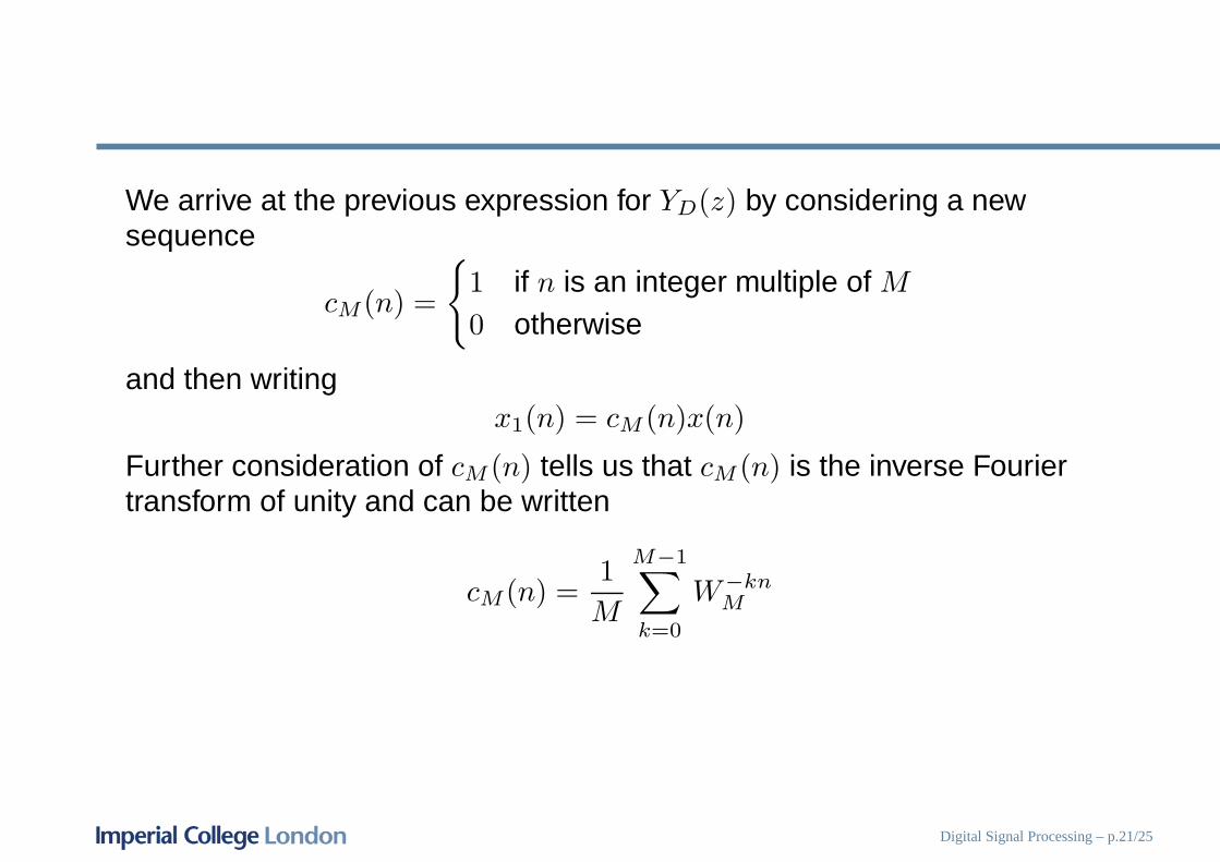
We arrive at the previous expression for YD(z) by considering a newsequence
cM (n) =
{
1 if n is an integer multiple of M
0 otherwise
and then writingx1(n) = cM (n)x(n)
Further consideration of cM (n) tells us that cM (n) is the inverse Fouriertransform of unity and can be written
cM (n) =1
M
M−1∑
k=0
W−knM
Digital Signal Processing – p.21/25
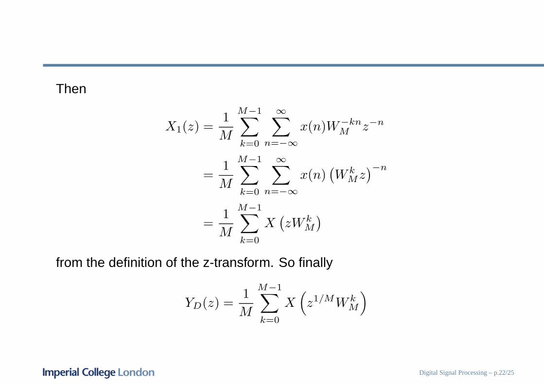
Then
X1(z) =1
M
M−1∑
k=0
∞∑
n=−∞
x(n)W−knM z−n
=1
M
M−1∑
k=0
∞∑
n=−∞
x(n)(
W kMz
)−n
=1
M
M−1∑
k=0
X(
zW kM
)
from the definition of the z-transform. So finally
YD(z) =1
M
M−1∑
k=0
X(
z1/MW kM
)
Digital Signal Processing – p.22/25
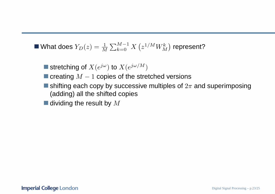
What does YD(z) = 1M
∑M−1k=0 X
(
z1/MW kM
)
represent?
stretching of X(ejω) to X(ejω/M)
creating M − 1 copies of the stretched versionsshifting each copy by successive multiples of 2π and superimposing(adding) all the shifted copiesdividing the result by M
Digital Signal Processing – p.23/25
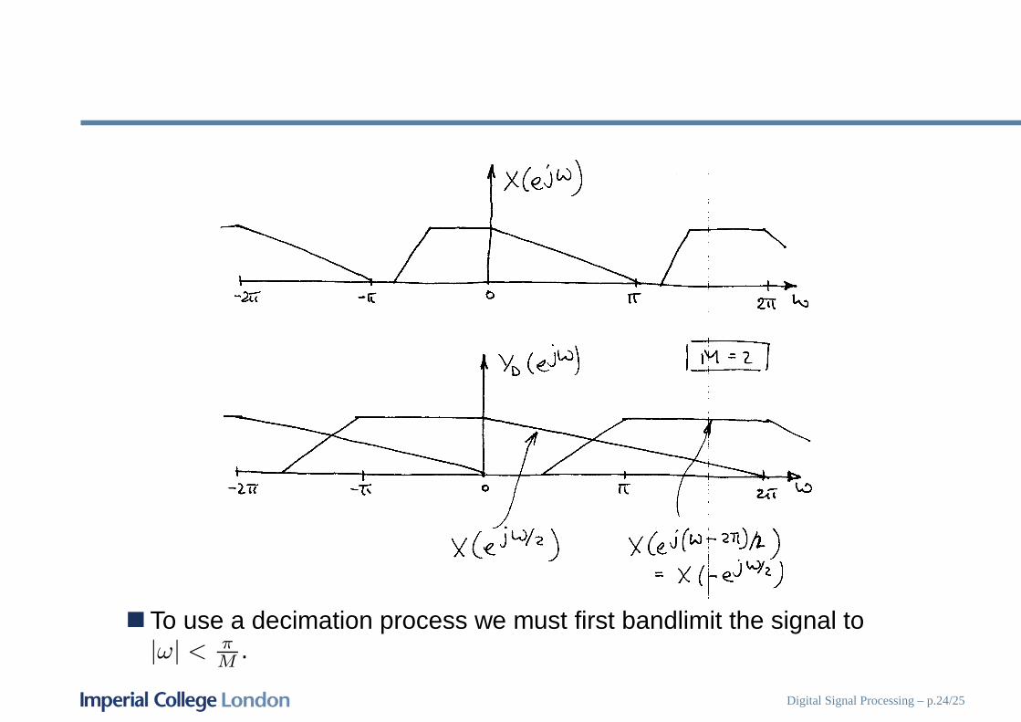
To use a decimation process we must first bandlimit the signal to|ω| < π
M .
Digital Signal Processing – p.24/25
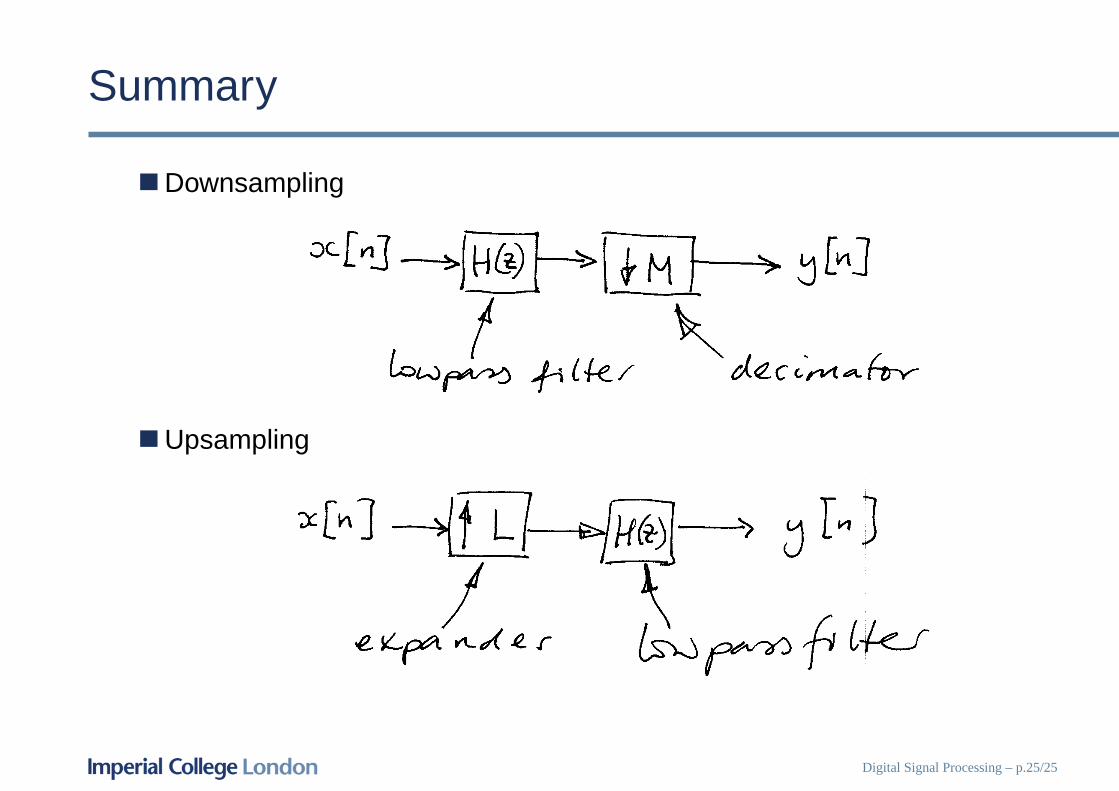
Summary
Downsampling
Upsampling
Digital Signal Processing – p.25/25