Testing the Conditional CAPM using GARCH-type Models

without any other Restrictions

M.B. Doolan and D.R. Smith

School of Economics and Finance, Queensland University of Technology

August 4, 2017

Abstract

We develop a new approach to testing conditional asset pricing models that avoids placing

restrictions on the price of risk. The only assumption made in the model is on the form

of the dynamics of the conditional covariance matrix of asset returns. Existing GARCH-

based models require an assumption on the price of risk, which we avoid in our approach. We

illustrate the methodology by testing a conditional version of the simple single-factor CAPM

using monthly returns and show that accounting for time varying betas using our preferred

model, which uses daily returns and accounts for the autocovariance in daily returns to

model conditional monthly volatilities, reduces average absolute alphas by 32% compared

with an unconditional model. Ultimately, we are unable to reject the null hypothesis that

the conditional CAPM prices the size and industry sorted portfolios but reject the model

for the Fama-French 25 portfolios.

Keywords

Conditional CAPM set

JEL Classification Numbers

C22, G00.

Corresponding author

M. B. Doolan

School of Economics and Finance

Queensland University of Technology

Brisbane, 4001

Qld, Australia

email m.doolan@qut.edu.au

Acknowledgments We thank Raymond Kan, seminar participants at the 2016

Princeton-QUT-SJTU-SMU Econometrics Conference (Shanghai) and seminar participants at

the Queensland University of Technology for their comments. Of course, all remaining errors

remain those of the authors.

1 Introduction

The Capital Asset Pricing Models (CAPM) of Sharpe (1964) and Lintner (1965) provides a

single state, single factor, general equilibrium theory of the risk-return relation. Despite some

initial empirical support, the weight of empirical evidence does not support the theory. For

example, studies find that CAPM’s single market factor cannot explain the returns of portfolios

formed on the basis of size, (Banz (1981)), book-to-market ratio (Fama and French, (1993))

or return momentum (Jegadeesh and Titman (1993)). With the presence of these so called

‘asset pricing anomalies’, the literature has advanced multi-factor asset pricing models that

include priced risk factor such as size, book-to-market and momentum; refer Carhart (1997) as

an example.

But before searching for additional factors that may explain asset returns, the failure to ac-

count for time-variation in the conditional distribution of asset returns should be considered.1

As highlighted by Lewellen and Nagel (2006) and others, the impact of failing to account for

conditional information produces biased estimates of the average pricing error (commonly refer

to as ‘alpha’). For example, if an asset’s conditional beta and market return positively (nega-

tively) covary, the estimated alpha is upwardly (downwardly) biased. Therefore, these simple

empirical and statistical facts, warrant the testing of the conditional CAPM.

Unfortunately for CAPM, the current state of empirical evidence does not support its conditional

version. Harvey (1989), one of the original tests of conditional CAPM, rejects the conditional

CAPM for the decile sorted size portfolios as the model’s pricing errors maintain a significant

amount of predictability, although it is noted that the all average pricing errors are insignificant

when tested individually and jointly. Interestingly, the insignificance of these alphas highlights

the alpha bias evident in other studies that have applied the unconditional CAPM to the size

portfolios. Despite these findings, the approach employed by Harvey (1989) and others including

Jagannathan and Wang (1996), and He, Kan, Ng and Zhang (1996) have been criticised for their

assumption that agents form their return expectations in relation to a set of state variables.

Therefore, as per Cochrane (2001), such tests of conditional CAPM are tests of the observed

stated state variables rather than conditional CAPM.

To avoid specifying a set of state variables in testing the conditional CAPM, Lewellen and

Nagel (2006) introduce a short window, non-overlapping, rolling regression approach to estimate

contemporaneous conditional alphas and betas. The approach assumes a stable joint distribution

within each short estimation window but allows for variation across sample windows. Therefore,

as the window rolls through time, a time-series of conditional alphas and betas are generated.

1Given that the holding period used for calculating returns to test CAPM are relatively short, e.g. daily ormonthly, the conditioning information is important relatively to longer term returns, refer Pagan (ref, p.30).

2

Significance tests of the estimated parameters can then be conducted in the Fama and Macbeth

(1973) framework. Their results indicates that the size anomaly is, at best, weak within the

conditional CAPM framework but the value and momentum anomalies remain significant.

A subsequent study by Boguth, Carlson, Fisher and Simutin (2011) that examined the Lewellen

and Nagel’s (2006) approach found that alphas were overstated because of an overconditioning

bias. They showed that the bias was essentially due to the short-run regressions using the

contemporaneous information set that is unknown to the investor under the conditional CAPM.

On correcting this bias with an instrumental variable approach, where the instrument may be

as simple as the lagged beta, Boguth et al. (2011) report alphas on the momentum portfolios

that were up to 30% smaller. Despite this decrease in alphas, they remained significant.

Another approach that avoids assumptions on the state variables is to directly model the con-

ditional moments of the joint distribution of asset returns and use these to infer the conditional

beta. Models such as the multivariate version of the autoregressive conditional heteroskedastici-

ty (ARCH) of Engle (1982) provide such capabilities. The initial applications of these models to

the asset pricing literature was Bollerslev, Engle and Wooldridge (1988) and recent extensions

include Bali and Engle (2010, 2014). These later of these studies offer similar findings to other

tests of the average pricing errors of the conditional CAPM in relation to size and momentum,

but Bali and Engle (2010, 2014) do report that the average pricing errors of the book-to-market

portfolios are insignificant. However, it is noted in applying the ARCH models, several impor-

tant restrictions are imposed to test the conditional CAPM. First, the joint distribution is often

limited to a bivariate distribution of the asset and market returns. While not problematic for

testing individual assets, it limits the ability of joint tests across assets. Second, in specifying

the conditional CAPM, the reward-to-risk ratio does not vary with time.

Following on from the literature, we propose a simple new approach to testing conditional

asset pricing models. The approach follows Lewellen and Nagel (2006), and Bali and Engle

(2010, 2014) in that it avoids the use of state variables. However, it contributes to the literature

by offering some specific improvements over these previous studies. First, as a test of the

conditional CAPM, it avoids making assumptions about the price-of-risk or the reward-to-risk

ratio by making all assumptions in relation to the modelling of the volatility dynamics. It

is argued, the success of volatility modelling relative to return modelling in finance warrants

this approach. Second, like Lewellan and Nagel (2006), we utilise high frequency information

when forming estimates of conditional betas and pricing errors but only employ information

within the agent’s information set. This is achieved by adapting the Mixed Data Sampling

(MIDAS) volatility modelling approach of Ghysels, Santa-Clara and Valkanov (2005a, 2005b)

to the multivariate setting. Third, we model the second conditional moment of the full asset

3

space in order to undertake a joint test of the significance across all portfolios. In doing so,

we derive and justify a new test statistic that only relies on conditional volatility estimates.

In addition, we specify the test statistic to account for parameter uncertainty in the volatility

models. Finally, our results support the findings of early studies in relation to the importance of

conditioning information to measuring pricing errors but we that this result is dependent on the

volatility model employed. Specifically, by using high frequency data, pricing errors are reduced

by up to 32%, which can be significant for the conclusions drawn for tests of the conditional

CAPM.

2 Tests of the Conditional CAPM

Following from Harvey (1989), the N asset multivariate conditional CAPM can be specified as

E [rt|Ωt−1] =E [rm,t|Ωt−1]

VAR [rm,t|Ωt−1]COV [rt, rm,t|Ωt−1] , (1)

where E [rt|Ωt−1] is N×1 vector of conditional expected excess asset returns, Ωt is the informa-

tion set from t − 1, E [rm,t|Ωt−1] and VAR [rm,t|Ωt−1] are scalars and measure the conditional

expected market return and variance, respectively, and COV [rt, rm,t|Ωt−1] is the N×1 vector of

conditional covariances between the return on each asset and the market. Defining the reward-

to-risk ratio as λ ≡ E[rm,t|Ωt−1]VAR[rm,t|Ωt−1] , which assumes λ is a constant, the model can be written

as

E [rt|Ωt−1] = λCOV [rt, rm,t|Ωt−1] . (2)

To test this model, Harvey (1989) applied a generalised method of moment framework and

assumed that the conditional expected return of the asset and the market were linear in a l× 1

vector of lagged state variables, Zt−1. As an example, one set of moments conditions used was

εt =

[ut

et

]=

[[rt − Zt−1δ]

[rt −α− λ (rmt − Zt−1δm) (rt − Zt−1δ)]

], (3)

where ut is a (N + 1)× 1 vector of ‘forecast’ errors and ut is a N × 1 vector of ‘pricing’ errors

while δ and δm coefficient matrices with (l ×N) and (l × 1), respectively. When these moment

conditions are interacted with the state variables, there are (2N + 1)×l orthogonality conditions

and (N + 1)× (1 + l) parameter to estimate. From this specification, the overall model can be

tested in an overidentifying restriction test while the restriction that α = 0 can also be tested.

To overcome the criticisms associated with using state variables, Lewellen and Nagel (2006)

directly estimate conditional alphas and betas from observed returns. In this instance, the

4

conditional CAPM is specified as

E [rt|Ωt−1] =COV [rt, rm,t|Ωt−1]

VAR [rm,t|Ωt−1]E [rm,t|Ωt−1] . (4)

Defining βt ≡ COV[rt,rm,t|Ωt−1]VAR[rm,t|Ωt−1] , the model can be written as,

E [rt|Ωt−1] = βtE [rm,t|Ωt−1] . (5)

Short window regressions are applied to a window of length τ where data is sampled at a

frequency t where t < τ . For example, using daily or weekly data, the regression for the ith

asset in a given quarter, τ is estimated as

ri,t = αi,τ + βi,τrm,t + εi,t (6)

The significance of the alphas is then tested in a Fama and MacBeth (1973) framework,

αi =1

T

T∑τ=1

αi,τ , VAR (αi) =1

T 2

T∑τ=1

(αi,τ − αi)2 . (7)

Although not tested directly by Lewellen and Nagel (2006), the Fama and MacBeth (1973)

framework is readily adjusted for the joint test that α = 0.

However, as identified by Boguth et al. (2011), this testing procedure suffers from an over-

conditioning bias as the conditional beta, βτ , and the market return rm,t are estimated from

information not contained within the investor’s information set, Ωt−1. As such, the mean of the

overconditioning bias is defined as

∆OCα ≡ −COV

[(βi,τ − βi,τ |t−1

), (rm,τ − rm,τ )

]. (8)

Boguth et al. (2011) highlight that as the sample size grows βi,τ |t−1 → βi,τ and the overcondi-

tioning bias should be small. Their empirical results show that correcting for the overcondition-

ing bias by using only information in the investor’s information set reduces estimated alphas by

between 20% and 40% on momentum portfolios.

Finally, the recent work of Bali and Engle (2010, 2014) has also investigated the validity of the

conditional CAPM using a bivariate GARCH in mean framework. Specifically, the system of

5

equations are

ri,t = αi + λhim,t +√hi,tui,t

rm,t = αm + λhm,t +√hm,tum,t

hi,t = ωi + αihi,t−1u2i,t−1 + βihi,t−1

hm,t = ωm + αmhm,t−1u2m,t−1 + βmhm,t−1

him,t = ρim,t√hi,t√hm,t

ρim,t =qim,t√

qii,t, qmm,t

qim,t = ρim + a1 (ui,t−1um,t−1 − ρim) + a2 (qim,t−1 − ρim)

where hi,t and hm,t are the conditional variances, him,t is the conditional covariance, ρim,t is the

conditional correlation, ui,t and um,t are standardised residuals while all remaining terms that

are not defined are parameters. As the Dynamic Conditional Correlation (DCC) model only

uses lagged information in forming conditional expectation, this approach does not suffer from

an overconditioning bias. In fact, Bali and Engle (2014) highlight this point by comparing their

GARCH based appraoch to that of Lewellen and Nagel (2006). However, it is noted that in

testing the pricing errors of the conditional CAPM that the approach assumes that the reward-

to-risk ratio, λ, is constant through time. Moreover, while Bali and Engle (2010) report a Wald

statistic for the joint test, no detail is provided on the calculation of this statistic. Despite these

perceived limiations, they find in support for the conditional CAPM in all but the momentum

portfolios.

3 A new test of the conditional CAPM

This paper proposes a new test of the conditional CAPM. The proposed test follows in the

spirit of Bali and Engle (2010,2014) in that it utilises multivariate volatility models to estimate

conditional betas given their success at modelling the conditional variance and covariance of

returns relative to models of the conditional mean. However, the novelty of this new test is

that it will a provide a joint test of the conditional CAPM that takes into consideration the

covariances between pricing errors.

To formulate the test, the setting includes N assets that aggregate to the market portfolio. The

N × 1 vector of asset returns from the conditional CAPM at time t is expressed as

rt = βt (θ) rm,t + et. (9)

where βt (θ) is formed from the conditional volatility models that are governed by a P × 1

6

parameter vector θ. If we follow a GMM specification and treat the volatility estimates as

primitive, the moment conditions for estimating the average pricing error can be written as

gt (α) = E [rt −α− βt (θ) rm,t] . (10)

Given the specification of these moment conditions and that the system is exactly identfied,

α = T−1∑T

t=1 et. To get the GMM standard errors, gt (α) is differentiated with respect to the

parameter vector,∂gt (α)

∂α= D = −IN , (11)

where IN is the N × N identity matrix. The efficient estimator of the asymptotic variance of

gt (α) is

S = E[ete′t

]−αα′. (12)

Under the null, S = E [ete′t], such that

COV (α) = T−1D−1SD−1 = T−1E[ete′t

]. (13)

In implementing this test, we note that as the N assets aggregate to the market portfolio,

the return on the market portfolio at time rm,t can be written as rm,t = w′t−1rt, where wt−1

previous periods N×1 vector of market value asset weights that sum to one. The N×N matrix

of conditional covariances of asset returns is defined as Σt. Given these inputs, the vector of

conditional covariances between asset and market returns is Σtwt−1 and the market variance is

w′tΣtwt. Then substituting terms into (9),

et =(IN −Σtwt−1

(w′t−1Σtwt−1

)−1w′t−1

)rt.

Solving for E [ete′t] and COV [α]

Et[ete′t

]=(IN −Σtwt−1

(w′t−1Σtwt−1

)−1w′t−1

)Et[rtr′t

] (IN −Σtwt−1

(w′t−1Σtwt−1

)−1w′t−1

)′= Σt −Σtwt

(w′tΣtwt

)−1w′tΣt

= Ωt

E[ete′t

]= Ω = T−1

T∑t=1

Ωt

COV [α] = T−1Ω

Finally, given the estimates of α and COV [α], the null hypothesis of no systematic pricing

7

errors is simply tested by the Wald test,

α′COV [α]−1α ∼ χ2m,

where there are m restrictions under the null.

In the above approach, the test statistic ignored uncertainty in estimates of the volatility pa-

rameter vector. In order to account for this uncertainty when computing the standard errors for

α, we introduce two derivations that produce the same result. Both note that we have already

estimated the volatility parameters using maximum likelihood, but we only present the first

approach here. The second approach is presented in Appendix A. Starting with,

∂ll (θ; rt)

∂θ= 0. (14)

We then introduce an expression

gt (θA) =

[dll(θ;rt)dθ

rt −α− βt (θ) rm,t

](15)

where θA is the (P +N) × 1 parameter vector for all volatility model parameters and alphas.

In undertaking this approach, it is observationally equivalent to setting α to a vector of N

zeros and using a weighting matrix that only weighted the first group of moments and using

the non-efficient weighted specification test. GMM standard errors are computed as

∂gt (θA)

∂θA= D =

[d2ll(θ;rt)dθdθ′ 0P×N

−∇βt · ft −IN

](16)

where ∇βt = dβt(θ)dθ′ is computed by numerically differentiating the function. A consistent

estimator can be formed by using the sample average of the product of the derivative of beta

with respect to the parameters times the factor return.2

To compute the standard errors of the estimates of α, we start with

COV (θA) = T−1D−1S(D′)−1

. (17)

The derivation of COV (θ) is presented in Appendix B. However, the 2,2 sub-matrix element

2It is trivial to extend for time-varying pricing errors by modelling them as αt = θα ·Zt−1 and replacing thesecond part of the moment conditions with (rt − θα ·Zt−1 − βt(θβ) · ft)⊗Zt−1.

8

corresponds to COV (α), which is

COV (α) =T−1

(Ω +∇βt · ftH−1IOPH

−1(∇βt · ft

)′+ T−1∂ll (θ, rt)

dθε′tH

−1(∇βt · ft

)′+ ∇βt · ftH−1T−1∂ll (θ, rt)

dθ′εt

).

(18)

The test statistic is then simply,

α′COV (α)−1α ∼ χ2N .

By accounting for parameter uncertainty in the volatility models, the covariance matrix for

the pricing errors includes adjustments for the covariance matrix of the maximum likelihood

estimates of the volatility parameters, H−1IOPH−1, plus an adjustment for the covariance

between the estimators.

4 Data

To apply and analyse our proposed approach to testing the conditional CAPM, portfolio returns

data, measured at daily and monthly frequencies, for the period 2 January 1958 to 30 December

2016 is obtained from Ken French’s data library http://mba.tuck.dartmouth.edu/pages/

faculty/ken.french/.3 The portfolios for which data are collected include: the decile sorted

size and industry portfolios and the Fama-French 25 (quintile, double sorted size and book-to-

market portfolios). Additional data is collected for the market value of each portfolio, average

firm size in each portfolio, the risk-free rate of return and the market return. In total, the daily

data series consists of 14,726 return observations for each portfolio while the equivalent monthly

data series has 702 return observations.

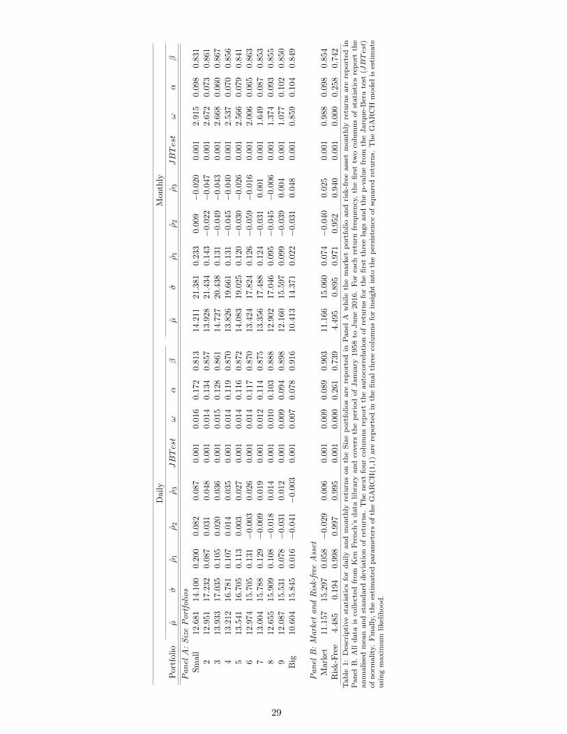
As an indication of the properties of the data collected, basic descriptive statistics on daily

and monthly returns on the size portfolios, market and risk-free asset are presented Table 1.

The size portfolio returns, refer Panel A, are consistent with the finance literature in that the

smallest firms generally display the greatest mean and standard deviation of returns, although

this decline is not always monotonic. The Jarque-Bera test rejects normality of returns and

there are some large return autocorrelations at the first lag for the smaller portfolios.

[INSERT TABLE 1 HERE]

3Ken French’s data library provides return data from 1 July 1926. However, the periods associated with thestock market crash of 1929, great depression, second world war and recovery period after the second world warare not include due to either their clearly excessive levels of volatility and the merger of CRSP and Compustatdatabases.

9

5 Size Results

5.1 Existing tests of unconditional and conditional CAPM

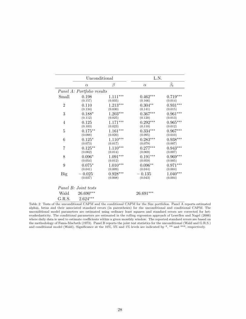
Table 2 presents parameter estimates and test results of the unconditional and conditional

CAPMs. The unconditional results of the individual portfolios presented in Panel A indicate

that alpha and beta tend to decrease in size, although not monotonically. Six of the estimated

alphas display some degree of statistical significance, which provides evidence against the un-

conditional CAPM. The joint tests in Panel B confirm this result as the unconditional CAPM

is rejected at the 1% level.

The remaining columns of Table 2 report test results of the conditional CAPM based on the

methodology of Lewellen and Nagel (2006). Clearly, the average αi and βi based on this method-

ology stand in stark contrast to their unconditional counterparts. All alphas are larger in mag-

nitude, generally by a factor of two or more, and almost all are highly significant. It is then

of no surprise that this significant under pricing is then evident through relatively small aver-

age betas. Moreover, the fact that the smallest betas are reported for the smaller portfolios

highlights a major disconnection between the unconditional and conditional models as reported

here. A comparison to results of Lewellen and Nagel (2006), albeit limited due to different

datasets and the fact they did not report results for monthly rolling regressions, show that the

alphas do somewhat reconcile. However, there is no reconciling the reported betas. Finally, and

unsurprisingly, the joint Wald test clearly rejects the conditional CAPM.

[INSERT TABLE 2 HERE]

5.2 New Test with Symmetric GARCH-type Models

Subsequent to the rejection of both the unconditional and conditional CAPMs, we then apply

our new estimation and testing approach to the conditional CAPM. The derivation of the alpha

estimate and joint test statistic in Section 3 did not rely on any specific model of multivariate

volatility. As such, a variety of volatility models could be used in testing the conditional CAPM.

An extensive literature on conditional volatility models exists and we leave reference of these

models to the detailed survey papers of Andersen, Bollerslev, Christoffersen & Diebold (2006),

Bauwens, Laurent & Rombouts (2006), and Silvennoinen & Terasvirta (2009). In this study,

we simply select a set of multivariate volatility models capable of modelling moderately sized

dimensions N ≤ 25 but of known varying quality. Our initial set of models, which we describe

in brief detail, are all symmetric in that volatility responds equally to positive and negative

returns of the same magnitude.

10

The first model used to capture the time-varying nature of volatility is a simple equally weighting

moving average (EQMA) model,

Ht =1

M

M∑j=1

εt−jε′t−j , (19)

where M is the number of observations within the window and εt−j is a lagged N ×1 demeaned

return vector. As the window moves through time, conditional volatility estimates change with

the addition of new information and the removal of the oldest information. For this study, we

set M = 60 as it corresponds to five years of monthly data.

The second model is the exponentially weighted average (EWMA) of RiskMetrics (1996). As

suggested by its name, this model employs an exponential weighting scheme that places greater

weight of more recent observations. Specifically,

Ht =∞∑j=1

λj−1 (1− λ) ε′t−jεt−j

= λHt−1 + (1− λ) εt−1ε′t−1,

where the parameter λ controls the decay weights. Following from RiskMetrics (1996), λ is set

at 0.97 for monthly data.

The third model is the Dynamic Conditional Correlation (DCC) of Engle (2002). The DCC pro-

vides a parametric alternative to the simple filters described above and, unlike other parametric

approaches, it can model the volatility dynamic in moderate dimensions, N ≤ 25, due to its

decomposition of the conditional covariance matrix into conditional volatility and conditional

correlation components,

Ht = DtRtDt (20)

where Dt is a N×N diagonal matrix of conditional standard deviations and Rt is a N×N , well-

defined, positive definite conditional correlation matrix. Through this decomposition, estimation

is performed with a two-step quasi-maximum likelihood procedure that first estimates each of

the conditional volatility equations and then subsequently estimates the conditional correlation

equation. Reference can be made to Engle and Sheppard (2001) for detail on this procedure.

A further benefit of this estimation approach is that a variety of conditional volatility and

correlation specifications can be used within DCC. To start, we model conditional volatility

with the classic GARCH(1,1) of Bollerslev (1986),

hi,t = ωi + αiε2i,t−1 + βihi,t−1, (21)

where ωi, αi and βi are parameters for each asset i. The conditional correlation is then modelled

11

with Engle’s (2002) mean reverting specification,

Qt = (1− α− β) Q + αzt−1z′t−1 + βQt−1 (22)

where α and β are parameters, Qt is a N × N matrix of conditional covariances of standard-

ised returns, which are zi,t−1 = εt−1√hi,t−1

, and Q is the unconditional covariance matrix of the

standardised returns. Finally, to ensure that correlations are well-defined on the main diagonal,

Rt = Q−1/2t QtQ

−1/2t . (23)

The final model considered is an extension of the Mixed Data Sampling (MIDAS) specification

of Ghysels, Santa-Clara and Valkanov (2005a, 2005b) to the multivariate space. There exists

several potential advantages of the MIDAS specification. First, it can use higher frequency data

when modelling a variable of interest that is observed or measured at a lower frequency. For

example, this study uses high frequency daily return data to estimate monthly volatility. The

perceived advantage of using this approach is twofold in that there is more data to estimate

the model and that more recent data is available. Finally, MIDAS provides a parsimonious

approach to estimating decay weights through its use of the beta or exponential functions.

To employ the MIDAS in the multivariate setting, we simply follow the DCC decomposition,

Ht = DtRtDt. Conditional variances are modelled in the standard MIDAS specification of

Ghysels, Santa-Clara and Valkanov (2005b), although we use the beta function rather than

the exponential function when estimating weights and allow for the scale parameter, φi, to be

estimated,

hi,t = φiΣkmax

k=0 b (k, θi,1; θi,2) ε2i,t−k. (24)

where b (k, θi,1; θi,2) is the beta function,

b (k, θi,1; θi,2) =f(

kkmax , θi,1; θi,2

)Σkmaxj=1 f

(j

kmax , θi,1; θi,2

) , (25)

where f (z, a, b) = za−1(1−z)b−1

β(a,b) where β (a, b) = Γ(a)Γ(b)Γ(a+b) , Γ is the gamma function and all weights

sum to one given the normalisation that occurs. When estimating the model, we restrict φi > 0,

θi,1 = 1 and θi,2 > 1. The later of these restrictions ensures that the beta function produces

a positive declining weighting scheme for lagged squared returns. Finally, we also estimate

the model with Ghysels, Santa-Clara and Valkanov (2005b) restriction that φi = 22, which is

consistent with assumption that returns are i.i.d.

12

The modelling of conditional correlation follows a similar process to that of the basic volatilities,

Qt = Σkmax

k=0 b (k, θ1; θ2) zt−kz′t−k. (26)

No scale parameter is required as it is redundant due the transformation Rt = Q−1/2t QtQ

−1/2t

and the θ parameters are restricted as above. In applying th maximum likelihood, only returns

at the lowest sampling frequency (e.g. monthly) are directly used to estimate the conditional

correlation equation. This ensures the internal consistency of the model as we cannot standard-

ised daily returns because we do not have estimates of daily conditional volatilities.

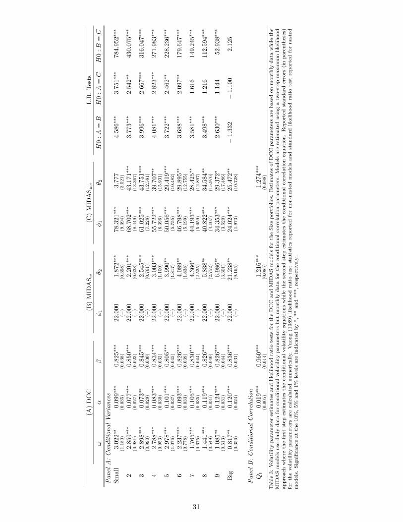
Parameter estimates and related statistics of the DCC and MIDAS models are presented in

Table 3. To distinguish between the two estimated MIDAS models, we refer to MIDAS model

where only the weight parameter is estimated as MIDASw and the one where both weight and

scale are estimated as MIDASws. Panel A of Table 3 shows that most estimated parameters

are significant. Interestingly, when the scale parameter is estimated for the MIDAS model, it

is always larger than 22 and in some instances it is more than three times larger. Formal tests

of the relative statistical quality of the volatility equations are conducted using the nested and

non-nested likelihood ratio tests described in Vuong (1989). These tests indicate that both

MIDAS specifications are rejected when tested against the simple GARCH model, although the

MIDASws is only rejected for the smaller portfolios. Relative to each other, MIDASws is clearly

the superior MIDAS specification. Interestingly, despite rejecting the restricted MIDAS model,

Panel B indicates that the choice of MIDAS specification has limited impact on the dynamics

of the correlation equation as the estimated parameters are almost identical.

Further evaluation of the parameters indicates a high level of persistence in volatility as the

sum of the GARCH(1,1) parameters αi and βi is close to one. Persistence within the MIDAS

specification is somewhat harder to identify given the scale parameter. However, the weighting

parameter provides some insight as larger parameters indicate less persistence with more weight

placed on more recent observations. From Panel A, it is then evident that the larger weighting

parameters for MIDASws places greater emphasis on the most recent observations.

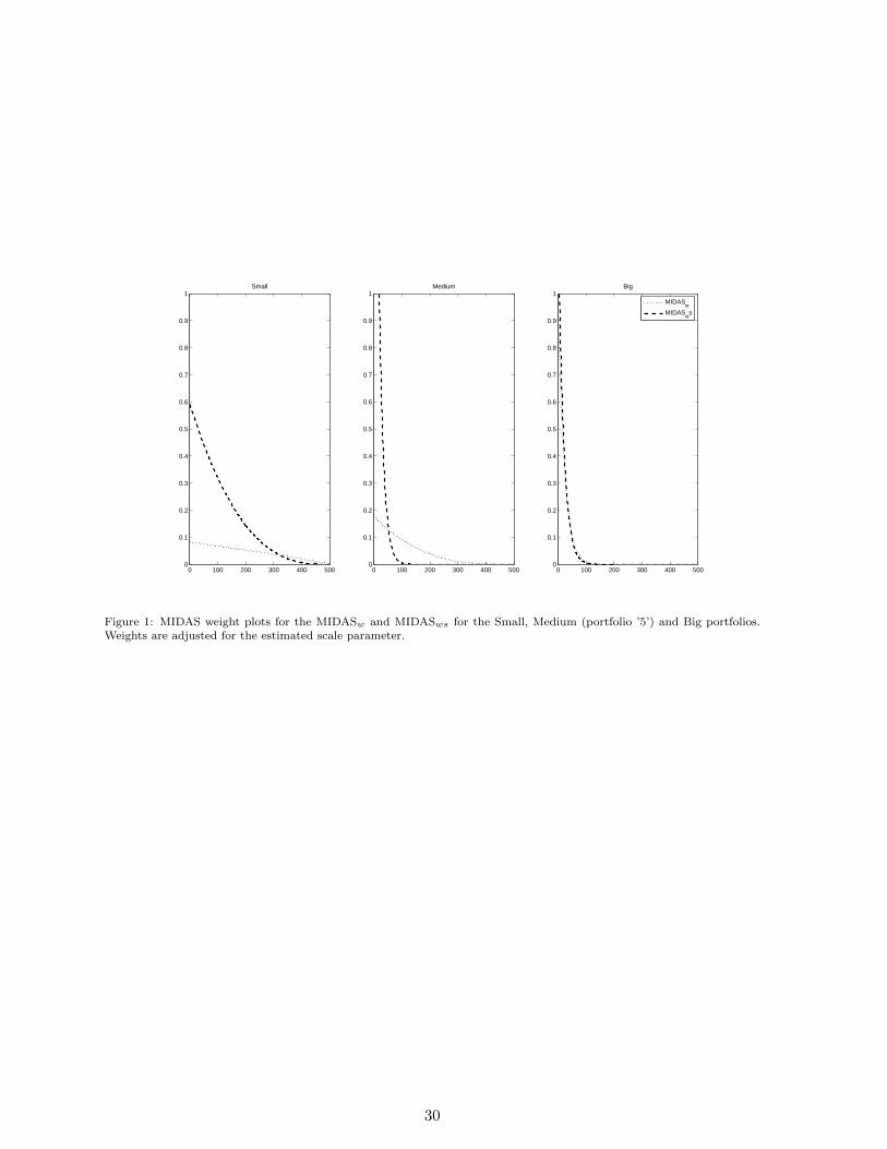
[INSERT TABLE 3 HERE]

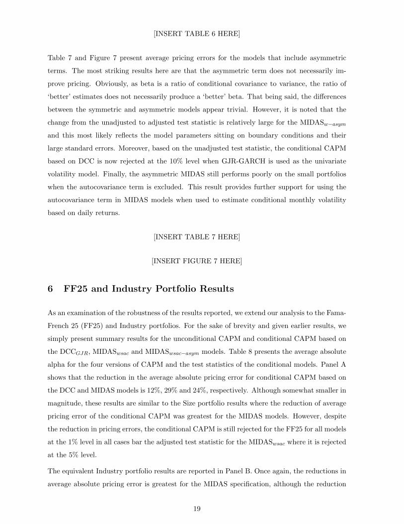
To see the full impact of the estimated parameters on the weighting functions, the scale term

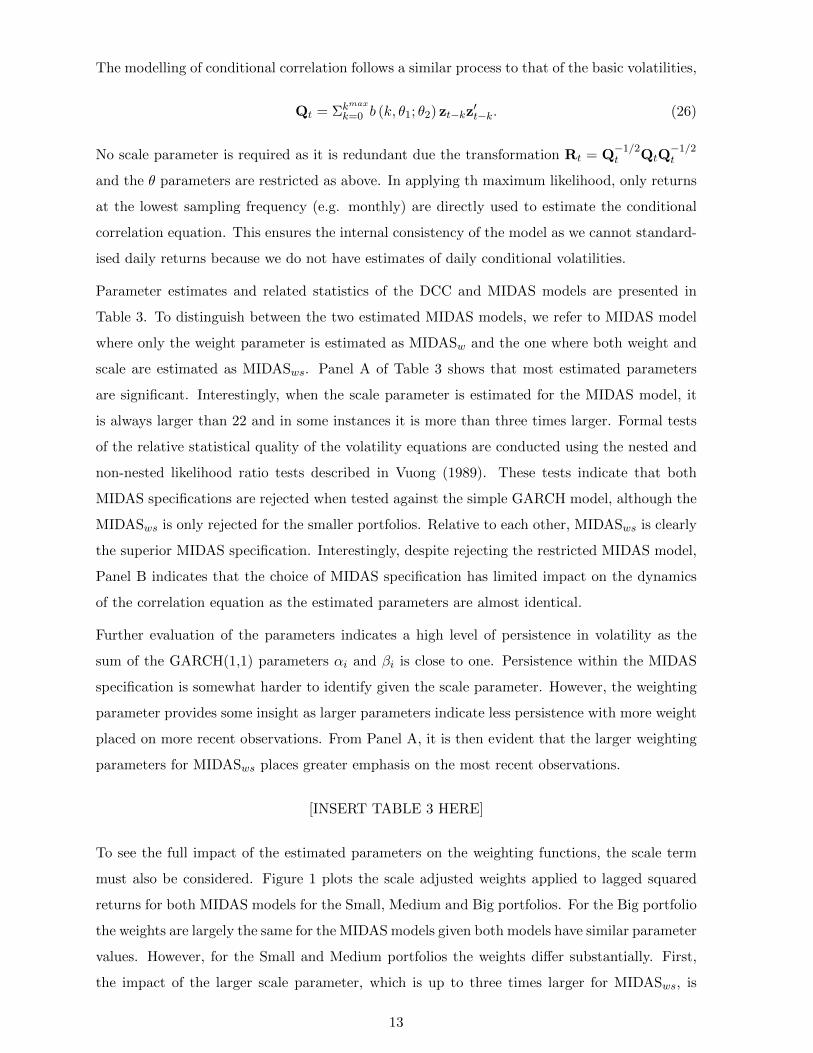
must also be considered. Figure 1 plots the scale adjusted weights applied to lagged squared

returns for both MIDAS models for the Small, Medium and Big portfolios. For the Big portfolio

the weights are largely the same for the MIDAS models given both models have similar parameter

values. However, for the Small and Medium portfolios the weights differ substantially. First,

the impact of the larger scale parameter, which is up to three times larger for MIDASws, is

13

clearly evident as the MIDASws places substantially more weight on lagged observations than

its restricted counterpart. Second, for the Medium portfolio, the larger weighting parameter

estimates have resulted in much more weight being placed on the most recent observations and

virtually all the weight is placed on the first 100 observations, which corresponds approximately

to the previous four months of observations. Given these plots and the likelihood ratio tests

reported above, it is concluded that the restriction that φi = 22 is too restrictive for all but the

largest of size portfolios.

[INSERT TABLE 1 HERE]

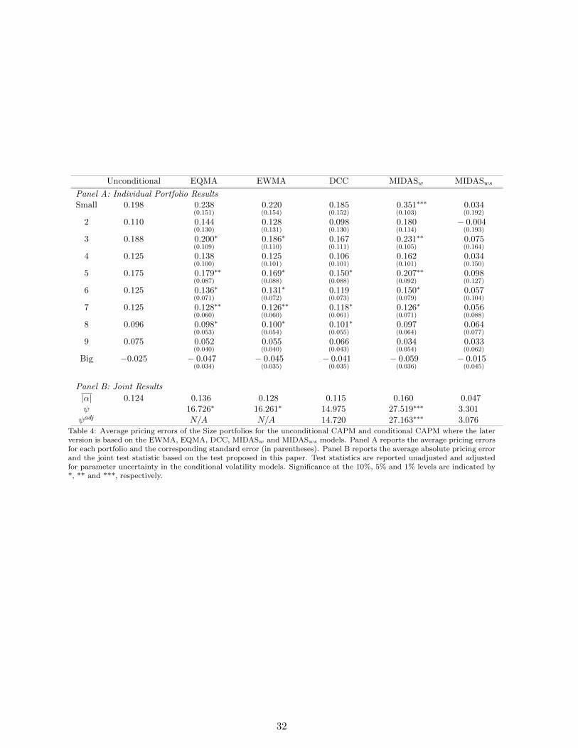
Table 4 reports average pricing errors and associated statistics for the conditional CAPM when

based on the EWMA, EQMA, DCC and MIDAS models. Panel A reports and tests the average

pricing errors of the individual size portfolios while Panel B reports the average absolute pricing

error across all portfolios and our new joint test statistics. The first result of note is that the

conditional CAPM based on the EQMA or EWMA models performs poorly across half of the

portfolios as the average pricing error of the conditional model is larger than equivalent one for

the unconditional model. Although the larger pricing error does not necessarily translate into

additional rejections of the model, the conditional CAPM is rejected for half of the portfolios.

The joint tests reported in Panel B confirm this result as the conditional CAPM is rejected at

the 10% level of significance for both EQMA and EWMA.

Results improve for the conditional CAPM when it is based DCC model. In Panel A, eight of

the ten portfolios now have smaller average pricing errors than the unconditional model and

only three are significant. Moreover, despite the overall decline in average absolute alpha being

a modest 7%, the joint tests do not reject the conditional CAPM based on DCC. Interestingly,

the similarity of the unadjusted and adjusted joint test statistics indicates that the effect of

parameter uncertainty in the volatility model is limited in this case.

The final results of Table 4 to report are those based on the MIDAS models. These results are

quite disparate and warrant some discussion. To start, the conditional CAPM based on the

MIDASw performs terribly on all but the largest of portfolios. When compared to the results

from the DCC based model, the pricing error can be up to twice the size and the overall average

absolute pricing error is approximately 50% larger. Individual and joint tests further highlight

this terrible performance as the conditional CAPM is rejected for most portfolios and the joint

tests are rejected at all conventional levels of significance. These results stand in stark contrast

to MIDASws. By simply providing flexibility in the scale parameter estimated, this MIDAS

specification produces the smallest average pricing errors for all portfolios, which results in

average absolute pricing error that is approximately 60% smaller than those of the unconditional

14

model and the conditional model based on DCC. Unsurprisingly, none of the individual tests or

the joint test statistics reject the conditional CAPM. In addition, the adjusted joint test indicates

that the test statistic is not overly sensitive to the volatility parameter estimates. Clearly, these

results indicate that the MIDAS model can reduce the pricing errors of the conditional CAPM,

although the MIDAS specification employed is of significance importance.

[INSERT TABLE 4 HERE]

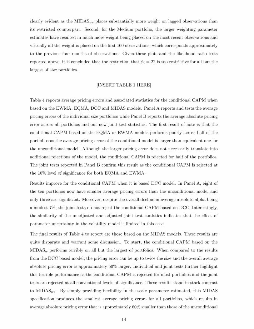
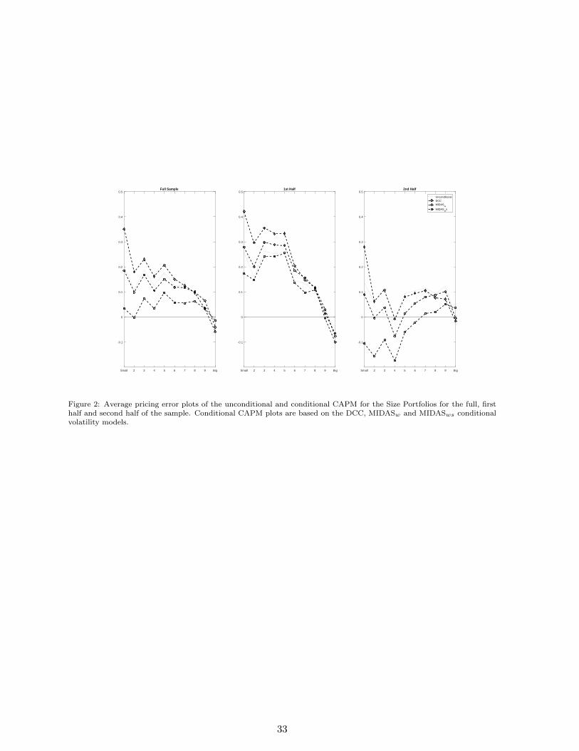
While the above results support the MIDASws version of the conditional CAPM, sub-sample

analysis indicates a significant flaw in the MIDASws model. Figure (2) plots the average pricing

errors of the unconditional CAPM and the conditional CAPM based on DCC, MIDASw and

MIDASws for the full sample, first half and second half of the samples in panels A, B and C,

respectively. What is evident from these plots is that MIDASws performs poorly in both halves

of the sample and that the small average pricing error of MIDASws over the full sample is not

driven by ‘better’ pricing per se. Instead, the full sample results are a direct result of excessive

over-pricing in the second half of the sample that has produced large negative pricing errors

for the smaller portfolios. The result of which is artificially low full sample results. Hence,

while MIDASws performed marginally better than other models in the first half of the sample,

we cannot conclude that it produces better results for the conditional CAPM given its relative

poor performance in the later half of the sample.

[INSERT FIGURE 2 HERE]

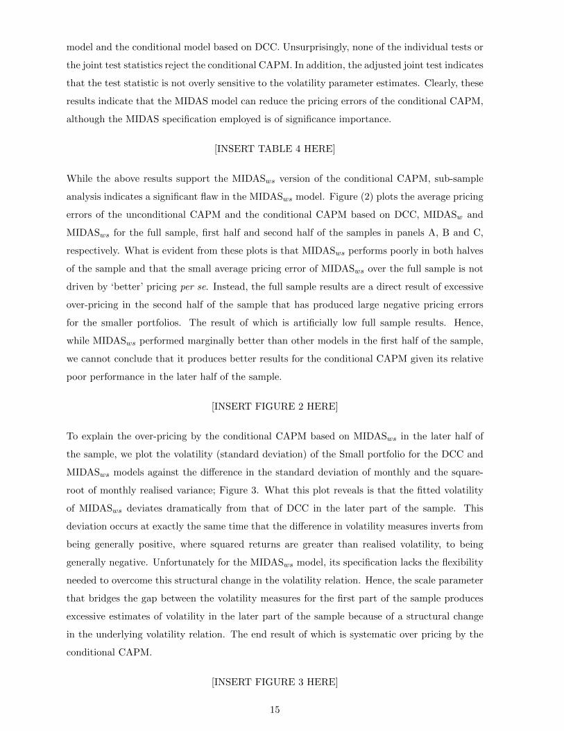
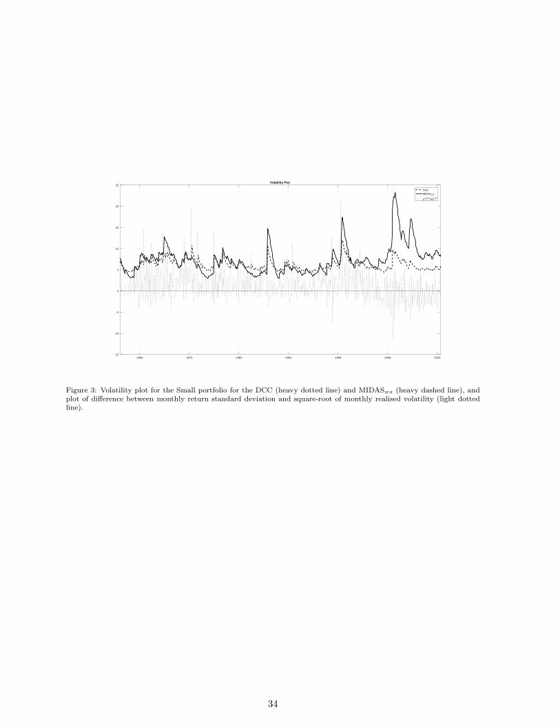
To explain the over-pricing by the conditional CAPM based on MIDASws in the later half of

the sample, we plot the volatility (standard deviation) of the Small portfolio for the DCC and

MIDASws models against the difference in the standard deviation of monthly and the square-

root of monthly realised variance; Figure 3. What this plot reveals is that the fitted volatility

of MIDASws deviates dramatically from that of DCC in the later part of the sample. This

deviation occurs at exactly the same time that the difference in volatility measures inverts from

being generally positive, where squared returns are greater than realised volatility, to being

generally negative. Unfortunately for the MIDASws model, its specification lacks the flexibility

needed to overcome this structural change in the volatility relation. Hence, the scale parameter

that bridges the gap between the volatility measures for the first part of the sample produces

excessive estimates of volatility in the later part of the sample because of a structural change

in the underlying volatility relation. The end result of which is systematic over pricing by the

conditional CAPM.

[INSERT FIGURE 3 HERE]

15

5.3 Testing with autocovariance corrected MIDAS

To overcome the problems of MIDASws in situations where the autocovariance of daily return

changes, we propose a simple adjustment. Specifically, following from French, Schwert and

Stamburg (1987), we include an autocovariance term for lagged returns in the MIDAS model

to help bridge the gap between squared monthly returns and the realised measure. Referring

to the model as MIDASwsac, where the additional ac in the subscript indicates an estimate for

autocovariance, we specify the model as

hi,t = φi,1Σkmax

k=0 b (k, θi,1; θi,2) ε2i,t−k + φi,2I0Σkmax−1

k=0 b (k, θi,3; θi,4) εi,t−kεi,t−k−1, (27)

where φi,2 is a strictly positive scale parameter and I0 is an indicator function that equals one

only when Σkmax−1k=0 b (k, θi,3; θi,4) εi,t−kεi,t−k−1 > 0 to ensure that variances remain positive. It

is noted that the indicator function still allows for negative values within the truncation period

as long as the weighted sum of all autocovariances is non-negative.

Table 5 reports the parameter estimates, average pricing errors and related statistics for the

MIDASwsac model. For this version of MIDAS, the autocovariance parameters are all signifi-

cant and their inclusion has a dramatic effect on the scale parameter. In particular, the scale

parameter on squared returns reduces for all portfolios and is never significantly larger than

22, although it is significantly smaller than 22 on three occasions. These results show that the

autocovariance term is an important as it captures part of the volatility dynamic that previously

was captured by the scale term. Figure 4 further highlights the value of the autocovariance term

by plotting the weights on lagged squared returns for the MIDASwsac and MIDASws models.

Consistent with reported parameter values, the Small portfolio sees a dramatic reduction in

weights with the inclusion of the autocovariance term while more modest reductions are noted

for the Medium and Big portfolios. Although the weights on the larger portfolios show modest

changes, the likelihood ratio tests reported in Table 5 show that the MIDASwsac specification

is superior to its restricted counterpart. Moreover, unlike earlier tests that the MIDASws was

inferior to the GARCH model, the non-nested likelihood ratio does not find that the MIDASwsac

is inferior to GARCH model. In fact, MIDASwsac is found to be superior for the Big portfolio.

In terms of average pricing errors, the average absolute alpha reported in Table 5 is larger than

spurious ones reported for MIDASws but, at 0.078, it is still 32% smaller than that reported for

DCC. Hence, it is of no surprise that joint tests cannot reject the conditional CAPM.

[INSERT TABLE 5 HERE]

[INSERT FIGURE 4 HERE]

16

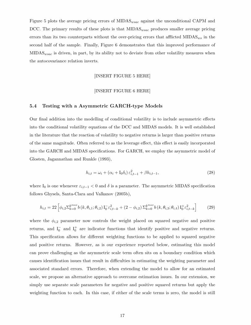
Figure 5 plots the average pricing errors of MIDASwsac against the unconditional CAPM and

DCC. The primary results of these plots is that MIDASwsac produces smaller average pricing

errors than its two counterparts without the over-pricing errors that afflicted MIDASws in the

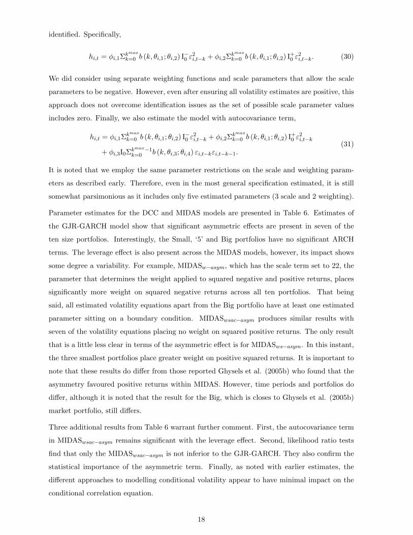
second half of the sample. Finally, Figure 6 demonstrates that this improved performance of

MIDASwsac is driven, in part, by its ability not to deviate from other volatility measures when

the autocovariance relation inverts.

[INSERT FIGURE 5 HERE]

[INSERT FIGURE 6 HERE]

5.4 Testing with a Asymmetric GARCH-type Models

Our final addition into the modelling of conditional volatility is to include asymmetric effects

into the conditional volatility equations of the DCC and MIDAS models. It is well established

in the literature that the reaction of volatility to negative returns is larger than positive returns

of the same magnitude. Often referred to as the leverage effect, this effect is easily incorporated

into the GARCH and MIDAS specifications. For GARCH, we employ the asymmetric model of

Glosten, Jagannathan and Runkle (1993),

hi,t = ωi + (αi + I0δi) ε2i,t−1 + βhi,t−1, (28)

where I0 is one whenever εi,t−1 < 0 and δ is a parameter. The asymmetric MIDAS specification

follows Ghysels, Santa-Clara and Valkanov (2005b),

hi,t = 22[φi,2Σkmax

k=0 b (k, θi,1; θi,2) I−0 ε2i,t−k + (2− φi,2) Σkmax

k=0 b (k, θi,3; θi,4) I+0 ε

2i,t−k

](29)

where the φi,2 parameter now controls the weight placed on squared negative and positive

returns, and I−0 and I+0 are indicator functions that identify positive and negative returns.

This specification allows for different weighting functions to be applied to squared negative

and positive returns. However, as is our experience reported below, estimating this model

can prove challenging as the asymmetric scale term often sits on a boundary condition which

causes identification issues that result in difficulties in estimating the weighting parameter and

associated standard errors. Therefore, when extending the model to allow for an estimated

scale, we propose an alternative approach to overcome estimation issues. In our extension, we

simply use separate scale parameters for negative and positive squared returns but apply the

weighting function to each. In this case, if either of the scale terms is zero, the model is still

17

identified. Specifically,

hi,t = φi,1Σkmax

k=0 b (k, θi,1; θi,2) I−0 ε2i,t−k + φi,2Σkmax

k=0 b (k, θi,1; θi,2) I+0 ε

2i,t−k. (30)

We did consider using separate weighting functions and scale parameters that allow the scale

parameters to be negative. However, even after ensuring all volatility estimates are positive, this

approach does not overcome identification issues as the set of possible scale parameter values

includes zero. Finally, we also estimate the model with autocovariance term,

hi,t = φi,1Σkmax

k=0 b (k, θi,1; θi,2) I−0 ε2i,t−k + φi,2Σkmax

k=0 b (k, θi,1; θi,2) I+0 ε

2i,t−k

+ φi,3I0Σkmax−1k=0 b (k, θi,3; θi,4) εi,t−kεi,t−k−1.

(31)

It is noted that we employ the same parameter restrictions on the scale and weighting param-

eters as described early. Therefore, even in the most general specification estimated, it is still

somewhat parsimonious as it includes only five estimated parameters (3 scale and 2 weighting).

Parameter estimates for the DCC and MIDAS models are presented in Table 6. Estimates of

the GJR-GARCH model show that significant asymmetric effects are present in seven of the

ten size portfolios. Interestingly, the Small, ‘5’ and Big portfolios have no significant ARCH

terms. The leverage effect is also present across the MIDAS models, however, its impact shows

some degree a variability. For example, MIDASw−asym, which has the scale term set to 22, the

parameter that determines the weight applied to squared negative and positive returns, places

significantly more weight on squared negative returns across all ten portfolios. That being

said, all estimated volatility equations apart from the Big portfolio have at least one estimated

parameter sitting on a boundary condition. MIDASwsac−asym produces similar results with

seven of the volatility equations placing no weight on squared positive returns. The only result

that is a little less clear in terms of the asymmetric effect is for MIDASws−asym. In this instant,

the three smallest portfolios place greater weight on positive squared returns. It is important to

note that these results do differ from those reported Ghysels et al. (2005b) who found that the

asymmetry favoured positive returns within MIDAS. However, time periods and portfolios do

differ, although it is noted that the result for the Big, which is closes to Ghysels et al. (2005b)

market portfolio, still differs.

Three additional results from Table 6 warrant further comment. First, the autocovariance term

in MIDASwsac−asym remains significant with the leverage effect. Second, likelihood ratio tests

find that only the MIDASwsac−asym is not inferior to the GJR-GARCH. They also confirm the

statistical importance of the asymmetric term. Finally, as noted with earlier estimates, the

different approaches to modelling conditional volatility appear to have minimal impact on the

conditional correlation equation.

18

[INSERT TABLE 6 HERE]

Table 7 and Figure 7 present average pricing errors for the models that include asymmetric

terms. The most striking results here are that the asymmetric term does not necessarily im-

prove pricing. Obviously, as beta is a ratio of conditional covariance to variance, the ratio of

‘better’ estimates does not necessarily produce a ‘better’ beta. That being said, the differences

between the symmetric and asymmetric models appear trivial. However, it is noted that the

change from the unadjusted to adjusted test statistic is relatively large for the MIDASw−asym

and this most likely reflects the model parameters sitting on boundary conditions and their

large standard errors. Moreover, based on the unadjusted test statistic, the conditional CAPM

based on DCC is now rejected at the 10% level when GJR-GARCH is used as the univariate

volatility model. Finally, the asymmetric MIDAS still performs poorly on the small portfolios

when the autocovariance term is excluded. This result provides further support for using the

autocovariance term in MIDAS models when used to estimate conditional monthly volatility

based on daily returns.

[INSERT TABLE 7 HERE]

[INSERT FIGURE 7 HERE]

6 FF25 and Industry Portfolio Results

As an examination of the robustness of the results reported, we extend our analysis to the Fama-

French 25 (FF25) and Industry portfolios. For the sake of brevity and given earlier results, we

simply present summary results for the unconditional CAPM and conditional CAPM based on

the DCCGJR, MIDASwsac and MIDASwsac−asym models. Table 8 presents the average absolute

alpha for the four versions of CAPM and the test statistics of the conditional models. Panel A

shows that the reduction in the average absolute pricing error for conditional CAPM based on

the DCC and MIDAS models is 12%, 29% and 24%, respectively. Although somewhat smaller in

magnitude, these results are similar to the Size portfolio results where the reduction of average

pricing error of the conditional CAPM was greatest for the MIDAS models. However, despite

the reduction in pricing errors, the conditional CAPM is still rejected for the FF25 for all models

at the 1% level in all cases bar the adjusted test statistic for the MIDASwsac where it is rejected

at the 5% level.

The equivalent Industry portfolio results are reported in Panel B. Once again, the reductions in

average absolute pricing error is greatest for the MIDAS specification, although the reduction

19

is a more modest 14%. That being said, the joint test statistics reveal that conditional CAPM

is only rejected when its estimates are from the DCC model. In part, these results reflect the

additional variation in pricing errors that comes from the MIDAS model. However, as most

examples have seen the MIDAS models produce the smallest average pricing errors, it is evident

that our conclusions come from an improvement in pricing accuracy, at least on average.

[INSERT TABLE 8 HERE]

7 Conclusion

This paper extends tests of the conditional CAPM based on GARCH type models such that

the test only makes assumptions on the volatility dynamics rather than the price of risk. In

doing so, the testing procedure avoids the over-conditioning bias of earlier papers by only using

information within the investor’s information set and removes limiting assumptions such as a

constant reward-to-risk ratio. A derivation of the Wald type test statistic is provided where the

test statistic does and does not account for uncertainty in the volatility parameter estimates.

Finally, the effect of the volatility model on the testing is considered.

Applied to the size sorted portfolios, several new and relevant results are evident. First, relative

to the unconditional alpha, the conditional alphas reported are up to 32% smaller. However,

this result is dependent on the choice in volatility model as this reduction is only reported for

the MIDAS model that employs daily return data, estimates a scale parameter and accounts

for the autocovariance in daily returns. The models that employ monthly returns show smaller

improvements, at best, over the unconditional model in terms of average pricing errors. However,

the improvement was sufficient enough for the conditional CAPM not to be rejected for the size

portfolios. Second, while parameter uncertainty of the volatility impacts the tests, its effects are

generally limited in most cases bar those where parameters are close to boundary conditions.

As such, the basic test statistic that treats volatility as known works reasonably well if one

considers that the parameters of the volatility model are reasonably well estimated. Finally,

consistent with other findings in the literature, the conditional CAPM cannot be rejected based

on tests of the average pricing errors of the size and industry portfolios but it is rejected for the

Fama-French 25 portfolio.

20

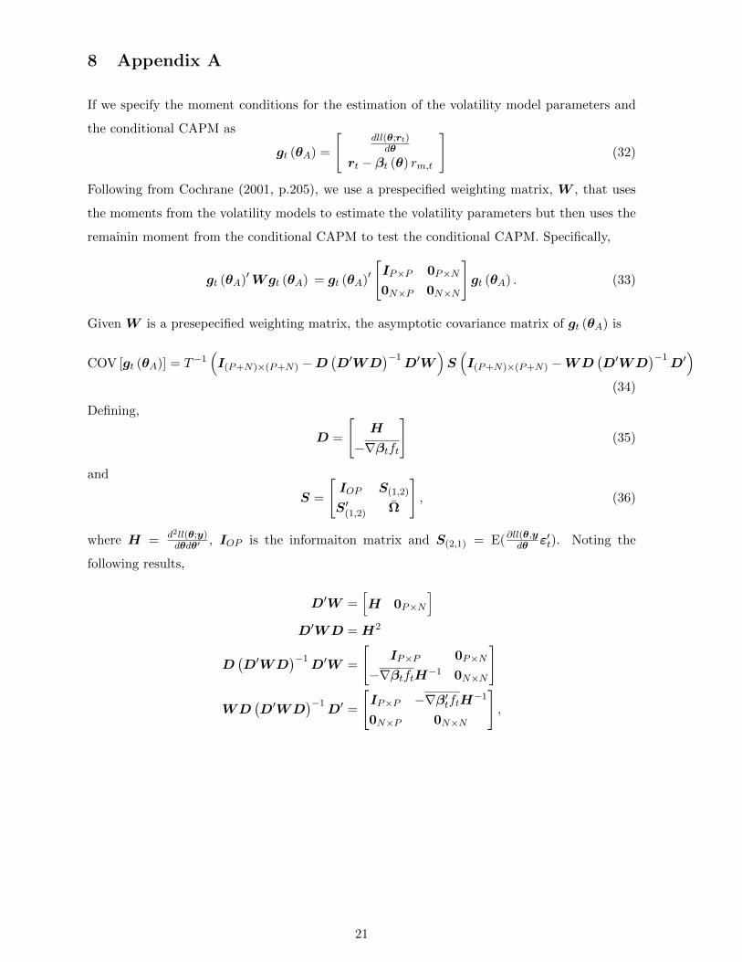
8 Appendix A

If we specify the moment conditions for the estimation of the volatility model parameters and

the conditional CAPM as

gt (θA) =

[dll(θ;rt)dθ

rt − βt (θ) rm,t

](32)

Following from Cochrane (2001, p.205), we use a prespecified weighting matrix, W , that uses

the moments from the volatility models to estimate the volatility parameters but then uses the

remainin moment from the conditional CAPM to test the conditional CAPM. Specifically,

gt (θA)′Wgt (θA) = gt (θA)′[IP×P 0P×N

0N×P 0N×N

]gt (θA) . (33)

Given W is a presepecified weighting matrix, the asymptotic covariance matrix of gt (θA) is

COV [gt (θA)] = T−1(I(P+N)×(P+N) −D

(D′WD

)−1D′W

)S(I(P+N)×(P+N) −WD

(D′WD

)−1D′)

(34)

Defining,

D =

[H

−∇βtft

](35)

and

S =

[IOP S(1,2)

S′(1,2) Ω

], (36)

where H = d2ll(θ;y)dθdθ′ , IOP is the informaiton matrix and S(2,1) = E(∂ll(θ,ydθ ε′t). Noting the

following results,

D′W =[H 0P×N

]D′WD = H2

D(D′WD

)−1D′W =

[IP×P 0P×N

−∇βtftH−1 0N×N

]

WD(D′WD

)−1D′ =

[IP×P −∇β′tftH−1

0N×P 0N×N

],

21

such that

COV [gt (θA)] = T−1

(I(P+N)×(P+N) −

[IP×P 0P×N

−∇βtftH−1 0N×N

])S

(I(P+N)×(P+N) −

[IP×P −∇β′tftH−1

0N×P 0N×N

])

= T−1

[0P×P 0P×N

∇βtftH−1 IN×N

][IOP S(1,2)

S′(1,2) Ω

][0P×P ∇β′tftH−1

0N×P IN×N

]

= T−1

[0P×P 0P×N

∇βtftH−1IOP + S′(1,2) ∇βtftH−1S(1,2) + Ω

][0P×P ∇β′tftH−1

IN×P 0N×N

]

= T−1

[0P×P 0P×N

0N×P ∇βtftH−1IOPH−1∇β′tft + S′(1,2)H

−1∇β′tft +∇βtftH−1S(1,2) + Ω

]

22

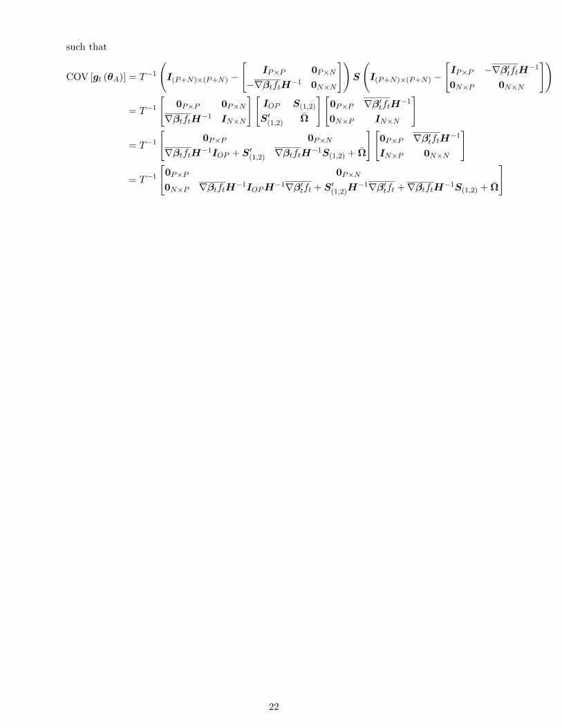
9 Appendix B

The inverse of the matrix D can be computed using the partitioned matrix inverse formula,

which simplifies greatly as the 1,2 term is zero. In fact we only need the lower row:

D−1(1,1) = H−1

where we are simplifying notation with

H =d2ll(θ;y)

dθdθ′.

D−1(2,2) = IN×N

D−1(1,2) = 0P×N

D−1(2,1) = −IN×N · ∇βt · ft ·H−1

We have the 2,2 sub-matrix giving

cov(α) = T−1[−∇βt · ft ·H−1, IN ] ·

[IOP S(1,2)

S′(1,2) Σ

]·

[−(∇βt · ft ·H−1)′

IN

]

, Where the moment variance-covariance matrix is given by

S =

[IOP S(1,2)

S′(1,2) Σ

]

and the off-diagonal term is

S(2,1) = E(∂ll(θ,y

dθε′t)

.

cov(α) = T−1[−∇βt · ft ·H−1 · IOP + S(2,1),−∇βt · ft · S(1,2) + Σ] ·

[−(∇βt · ft ·H−1)′

IN

]

so we have

cov(α) = T−1(Σ +∇βt · ft ·H−1 · IOP ·H−1 · (∇βt · ft)′ + S(2,1) ·H−1 · (∇βt · ft)′ −∇βt · ft · S(1,2)

)The terms following the Σ account for parameter uncertainty, as if we knew the parameters

driving the dynamics of the conditional βts then the covariance matrix of the sample abnormal

returns will simply be T−1Σ.

cov(α) = T−1(Σ +∇βt · ft · cov(θMLE) · (∇βt · ft)′ + S(2,1) ·H−1 · (∇βt · ft)′ −∇βt · ft ·H−1 · S(1,2)

)

23

The presence of the covariance matrix of the MLE parameter estimates driving the dynamics

of θ helps make this point more clearly. So the variance of the abnormal returns equals the

variance of the pricing errors if we new the betas exactly plus a delta method adjustment for the

estimation error in the parameter estimates, plus an adjustment for the covariance between the

estimators. This will produce larger standard errors because we need to estimate the parameters

driving the beta dynamics.

24

References

Andersen, T.G., Bollerslev, T., Christoffersen, P.F. & Diebold, F.X. (2006). Volatility and Cor-

relation Forecasting. In: Elliot, G., Granger, C.W.J. and Timmerman, A., (Eds.), Handbook

of Economic Forecasting. Elsevier, Burlington.

Bali, T. G. & Engle, R. F. (2010). Resurrecting the conditional CAPM with dynamic condi-

tional correlations. Working Paper, New York, New York University.

Bali, T. G. & Engle, R. F. (2014). The conditional CAPM explains the value premium. Working

Paper, New York, New York University.

Banz, R. W. (1981). The relationship between return and market value of common stocks.

Journal of Financial Economics, 9, 318.

Bauwens, L., Laurent, S. & Rombouts, V. K. (2006). Multivariate GARCH models: A review.

Journal of Applied Econometrics, 21, 79-109.

Boguth, O., Carlson, M., Fisher, A., & Simutin, M. (2011). Conditional risk and performance

evaluation: Volatility timing, overconditioning, and new estimates of momentum alpha. Journal

of Financial Economics, 102, 363389.

Bollerslev, T. (1986). Generalized autoregressive conditional heteroskedasticity. Journal of E-

conometrics, 31, 307-327.

Bollerslev, T., Engle. R. F. & Wooldridge, J. M. (1988). A capital asset pricing model with

time-varying covariances. The Journal of Political Economy, 96, 116-131.

Carhart, M. M. (1997). On persistence in mutual fund performance. Journal of Finance, 52,

pp. 57-82.

Cochrane, J. (2001). Asset Pricing. Princeton University Press, Princeton, NJ

Engle, R.F. (1982). Autoregressive conditional heteroskedasticity with estimates of the variance

of U.K. inflation. Econometrica, 50, 987-1008.

Engle, R.F. (2002). Dynamic conditional correlation: A simple class of multivariate general-

ized autoregressive conditional heteroskedasticity models. Journal of Business and Economic

Statistics, 20, 339-350.

Engle, R. F. & Sheppard, K. (2001). Theoretical and empirical properties of dynamic condi-

tional correlation multivariate GARCH. Working Paper, San Diego, University of California

San Diego.

25

Fama, E. F.& French, K. R. (1993). Common risk factors in the returns on stocks and bonds.

Journal of Financial Economics, 33, 3-56.

Fama, E. & MacBeth, J. (1973). Risk, return and equilibrium: empirical tests. Journal of

Political Economy 81, 607636.

Ferson, W.E. & Harvey, C. R. (1999). Conditioning variables and the cross section of stock

returns. The Journal of Finance, 54, 1325-1360.

French, K. R., Schwert, G. W. & Stambaugh R. F. (1987). Expected stock return and volatility,

Journal of Financial Economics, 19, 3-29.

Gibbons, M. R., Ross, S. A. & Shanken, J. (1989). Test of the efficiency of a given portfolio.

Econometrica, , 1121-1152.

Ghysels, E., Santa-Clara, P. & Valkanov, R. (2005). Predicting volatility: getting the most out

of return data sampled at different frequencies. Journal of Econometrics, 131, 59-95.

Ghysels, E., Santa-Clara, P. & Valkanov, R. (2005). There is a risk-return trade-off after all.

Journal of Financial Economics, 76, 509548.

Glosten, L. R., Jagannathan, R. & Runkle, D. E. (1993). On the relation between the expected

value and the volatility of the nominal excess return on stocks. Journal of Finance, 48, 1779-

1801.

Harvey, C. R. (1989). Time-varying conditional covariance in tests of asset pricing models.

Journal of Financial Economics, 24, 289-317.

He J., Kan, R., Ng, L. & Zhang, C. (1996). Tests of the relations among marketwide factors,

firmspecific variables, and stock returns using a conditional asset pricing model, 51, 1891-1908.

Jagannathan, R., Wang, W. (1996). The conditional CAPM and the cross-section of stock

returns. Journal of Finance 51, 353.

Jegadeesh, N. & Titman, S. (1993). Returns to buying winners and selling losers: Implications

for stock market efficiency. Journal of Finance, 48, 65-91.

Lewellen J. & Nagel S. (2006). The conditional CAPM does not explain asset-pricing anomalies.

Journal of Financial Economics, 82, 289-314.

Lintner, J. (1965). The valuation of risk assets and the selection of risky investment in stock

portfolios and capital budgets. Review of Economics and Statistics, 47, 13-37.

Riskmetrics. (1996). Technical document, New York: JP Morgan/Reuters.

26

Sharpe, W. F. (1964). Capital asset prices: A theory of market equilibrium under conditions

of risk. Journal of Finance, 19, 425-442.

Silvennoinen, A. & Terasvirta, T., (2009). Multivariate GARCH models. In: Andersen, T.G.,

Davis, R.A., Kreiss, J.P. and Mikosch (Eds.), Handbook of Financial Time Series. Berlin:

Springer-Verlag, pp. 201-229.

Tse, Y.K. & Tsui, A. K. C. (2002). A multivariate GARCH model with time-varying correla-

tions. Journal of Business and Economic Statistics, 20, 351-362.

Vuong, Q. H. (1989). Likelihood ratio rests for model selection and non-nested hypotheses.

Econometrics, 57, 307-333.

27

Unconditional L.N.

α β α βt

Panel A: Portfolio resultsSmall 0.198

(0.157)1.111∗∗∗(0.035)

0.462∗∗∗(0.166)

0.719∗∗∗(0.014)

2 0.110(0.134)

1.213∗∗∗(0.030)

0.304∗∗(0.141)

0.931∗∗∗(0.015)

3 0.188∗(0.112)

1.203∗∗∗(0.025)

0.367∗∗∗(0.120)

0.961∗∗∗(0.013)

4 0.125(0.103)

1.171∗∗∗(0.023)

0.292∗∗∗(0.110)

0.965∗∗∗(0.012)

5 0.175∗∗(0.088)

1.161∗∗∗(0.020)

0.334∗∗∗(0.095)

0.967∗∗∗(0.010)

6 0.125∗(0.073)

1.110∗∗∗(0.017)

0.283∗∗∗(0.079)

0.938∗∗∗(0.007)

7 0.125∗∗(0.062)

1.110∗∗∗(0.014)

0.277∗∗∗(0.069)

0.943∗∗∗(0.007)

8 0.096∗(0.054)

1.091∗∗∗(0.012)

0.191∗∗∗(0.059)

0.969∗∗∗(0.005)

9 0.075∗(0.041)

1.010∗∗∗(0.009)

0.096∗∗(0.044)

0.971∗∗∗(0.004)

Big − 0.025(0.037)

0.928∗∗∗(0.008)

− 0.135(0.043)

1.040∗∗∗(0.004)

Panel B: Joint testsWald 26.690∗∗∗ 26.691∗∗∗

G.R.S. 2.624∗∗∗

Table 2: Tests of the unconditional CAPM and the conditional CAPM for the Size portfolios. Panel A reports estimatedalphas, betas and their associated standard errors (in parentheses) for the unconditional and conditional CAPM. Theunconditional model parameters are estimated using ordinary least squares and standard errors are corrected for het-eroskedasticity. The conditional parameters are estimated in the rolling regression approach of Lewellen and Nagel (2006)where daily data is used to estimate coefficients within a given monthly window. The reported standard errors are based onthe methodology of Fama-Macbeth (1973). Panel B reports the joint test statistics for the unconditional (Wald and G.R.S.)and conditional model (Wald). Significance at the 10%, 5% and 1% levels are indicated by *, ** and ***, respectively.

28

Dai

lyM

onth

ly

Port

folio

µσ

ρ1

ρ2

ρ3

JBTest

ωα

βµ

σρ

1ρ

2ρ

3JBTest

ωα

β

Panel

A:SizePortfolios

Sm

all

12.6

8114.1

000.

200

0.08

20.

087

0.0

01

0.0

160.

172

0.81

314.2

1121.3

810.

233

0.00

9−

0.02

00.0

012.9

150.

098

0.83

12

12.

951

17.2

320.

087

0.031

0.04

80.

001

0.0

140.

134

0.85

713.9

2821.4

340.

143−

0.0

22−

0.0

470.0

012.6

72

0.07

30.

861

313.9

3317.

035

0.10

50.

020

0.03

60.

001

0.0

150.

128

0.86

114.7

2720.4

380.

131−

0.04

9−

0.0

430.0

012.6

680.

060

0.867

413.2

12

16.

781

0.10

70.

014

0.03

50.

001

0.0

140.

119

0.87

013.8

2619.6

610.

131−

0.04

5−

0.0

400.0

012.5

370.

070

0.85

65

13.5

4116.

705

0.11

30.

003

0.02

70.

001

0.0

140.

116

0.87

214.0

8319.0

250.

120−

0.03

0−

0.0

260.0

012.5

660.

079

0.84

16

12.9

74

15.7

050.

131

−0.

003

0.02

60.

001

0.0

140.

117

0.87

013.4

2417.8

240.

126−

0.05

9−

0.0

160.0

012.0

06

0.065

0.86

37

13.0

0415.

788

0.12

9−

0.009

0.01

90.

001

0.0

120.

114

0.87

513.3

5617.4

880.

124−

0.03

10.

001

0.00

11.6

49

0.08

70.

853

812.6

55

15.

909

0.10

8−

0.018

0.01

40.

001

0.0

100.

103

0.88

812.9

0217.0

460.

095−

0.04

5−

0.0

060.0

011.3

74

0.09

30.

855

912.0

8715.

531

0.07

8−

0.0

310.

012

0.00

10.0

090.

094

0.89

812.1

6015.5

970.

099−

0.03

90.

004

0.00

11.0

770.

102

0.85

0B

ig10.6

04

15.

845

0.01

6−

0.0

41−

0.00

30.0

010.0

070.

078

0.91

610.4

1314.3

710.

022−

0.03

10.

048

0.00

10.8

590.

104

0.84

9

Panel

B:Market

andRisk-free

Asset

Mar

ket

11.1

57

15.

297

0.05

8−

0.0

290.

006

0.00

10.0

090.

089

0.90

311.1

6615.0

600.

074−

0.04

00.

025

0.00

10.9

880.

098

0.85

4R

isk-F

ree

4.48

50.

194

0.998

0.99

70.

995

0.00

10.0

000.

261

0.73

94.

495

0.89

50.

971

0.95

20.

940

0.00

10.0

00

0.258

0.742

Tab

le1:

Des

crip

tive

stati

stic

sfo

rd

aily

an

dm

onth

lyre

turn

son

the

Siz

ep

ort

folios

are

rep

ort

edin

Pan

elA

wh

ile

the

mark

etp

ort

foli

oan

dri

sk-f

ree

ass

etm

onth

lyre

turn

sare

rep

ort

edin

Pan

elB

.A

lld

ata

isco

llec

ted

from

Ken

Fre

nch

’sd

ata

lib

rary

an

dco

ver

sth

ep

erio

dof

Janu

ary

1958

toJu

ne

2016.

For

each

retu

rnfr

equ

ency

,th

efi

rst

two

colu

mn

sof

stati

stic

sre

port

the

an

nu

alise

dm

ean

an

dst

an

dard

dev

iati

on

of

retu

rns.

Th

en

ext

fou

rco

lum

ns

rep

ort

the

au

toco

rrel

ati

on

of

retu

rns

for

the

firs

tth

ree

lags

an

dth

ep

-valu

efr

om

the

Jarq

ue-

Ber

ate

st(JBTest)

of

norm

ality

.F

inally,

the

esti

mate

dp

ara

met

ers

of

the

GA

RC

H(1

,1)

are

rep

ort

edin

the

fin

al

thre

eco

lum

ns

for

insi

ght

into

the

per

sist

ence

of

squ

are

dre

turn

s.T

he

GA

RC

Hm

od

elis

esti

mate

usi

ng

maxim

um

likel

ihood

.

29

0 100 200 300 400 5000

0.1

0.2

0.3

0.4

0.5

0.6

0.7

0.8

0.9

1Small

0 100 200 300 400 5000

0.1

0.2

0.3

0.4

0.5

0.6

0.7

0.8

0.9

1Medium

0 100 200 300 400 5000

0.1

0.2

0.3

0.4

0.5

0.6

0.7

0.8

0.9

1Big

MIDAS

w

MIDASw

s

Figure 1: MIDAS weight plots for the MIDASw and MIDASws for the Small, Medium (portfolio ’5’) and Big portfolios.Weights are adjusted for the estimated scale parameter.

30

(A)

DC

C(B

)M

IDA

Sw

(C)

MID

ASws

L.R

.T

ests

ωα

βφ

1θ 2

φ1

θ 2H

0:A

=B

H0

:A

=C

H0

:B

=C

Panel

A:ConditionalVariances

Sm

all

3.02

2∗∗

(1.1

80)

0.0

99∗∗∗

(0.0

35)

0.82

5∗∗∗

(0.0

38)

22.0

00(−

)1.8

72∗∗∗

(0.3

98)

78.3

21∗∗∗

(9.3

94)

3.7

77(3.5

21)

4.58

6∗∗∗

3.75

1∗∗∗

784.9

52∗∗∗

22.

859∗∗∗

(0.9

81)

0.0

77∗∗∗

(0.0

27)

0.85

0∗∗∗

(0.0

23)

22.0

00(−

)2.2

01∗∗∗

(0.6

38)

68.

702∗∗∗

(8.4

49)

43.1

71∗∗∗

(13.3

67)

3.773∗∗∗

2.542∗∗

430.0

75∗∗∗

32.

898∗∗∗

(0.9

90)

0.0

73∗∗

(0.0

29)

0.84

5∗∗∗

(0.0

30)

22.0

00

(−)

2.5

45∗∗∗

(0.7

61)

61.0

25∗∗∗

(7.2

28)

43.7

51∗∗∗

(12.5

81)

3.9

96∗∗∗

2.66

7∗∗∗

316.0

47∗∗∗

42.

788∗∗∗

(0.9

53)

0.0

83∗∗∗

(0.0

30)

0.83

4∗∗∗

(0.0

32)

22.0

00(−

)3.

003∗∗∗

(1.1

00)

55.7

22∗∗∗

(6.3

96)

39.

707∗∗

(15.9

31)

4.0

81∗∗∗

2.823∗∗∗

271.9

83∗∗∗

52.

978∗∗∗

(1.0

76)

0.1

01∗∗∗

(0.0

37)

0.80

5∗∗∗

(0.0

45)

22.0

00(−

)3.

990∗∗

(1.8

17)

50.0

56∗∗∗

(5.7

55)

29.

419∗∗∗

(10.4

82)

3.7

22∗∗∗

2.4

62∗∗

228.2

36∗∗∗

62.

237∗∗∗

(0.7

78)

0.09

3∗∗∗

(0.0

33)

0.82

6∗∗∗

(0.0

39)

22.0

00

(−)

4.08

9∗∗

(1.8

38)

46.7

98∗∗∗

(5.1

99)

29.8

95∗∗

(12.7

55)

3.6

88∗∗∗

2.0

97∗∗

179.6

47∗∗∗

71.

765∗∗∗

(0.6

75)

0.10

5∗∗∗

(0.0

35)

0.83

0∗∗∗

(0.0

44)

22.

000

(−)

4.366∗

(2.5

35)

44.

193∗∗∗

(5.0

59)

28.

425∗∗

(12.8

97)

3.5

81∗∗∗

1.6

16149.

245∗∗∗

81.

441∗∗∗

(0.5

49)

0.11

9∗∗∗

(0.0

31)

0.8

26∗∗∗

(0.0

40)

22.0

00(−

)5.

838∗∗

(2.7

52)

40.8

22∗∗∗

(4.1

07)

34.5

84∗∗

(15.9

76)

3.4

98∗∗∗

1.2

16

112.

594∗∗∗

91.

085∗∗

(0.5

13)

0.12

4∗∗∗

(0.0

31)

0.8

26∗∗∗

(0.0

44)

22.

000

(−)

6.986∗∗

(3.3

01)

34.3

53∗∗∗

(3.5

20)

29.

372∗

(17.4

86)

2.6

30∗∗∗

1.1

4452.

938∗∗∗

Big

0.81

7∗∗

(0.3

56)

0.12

0∗∗∗

(0.0

24)

0.8

36∗∗∗

(0.0

31)

22.0

00

(−)

21.2

38∗∗

(9.1

65)

24.0

24∗∗∗

(1.9

73)

25.4

72∗∗

(10.7

28)

−1.

332

−1.1

002.

125

Panel

B:ConditionalCorrelation

Qt

0.01

9∗∗∗

(0.0

05)

0.9

60∗∗∗

(0.0

14)

1.2

16∗∗∗

(0.0

85)

1.274∗∗∗

(0.0

88)

Tab

le3:

Vola

tility

para

met

eres

tim

ate

sand

likel

ihood

rati

ote

sts

for

the

DC

Can

dM

IDA

Sm

od

els

for

the

Siz

ep

ort

folios.

Est

imate

sof

DC

Cp

ara

met

ers

are

base

don

month

lyd

ata

wh

ile

the

MID

AS

mod

els

use

daily

data

for

con

dit

ion

al

vola

tility

para

met

ers

bu

tm

onth

lyd

ata

for

the

con

dit

ion

al

corr

elati

on

para

met

ers.

Mod

els

are

esti

mate

du

sin

ga

two-s

tep

maxim

um

likel

ihood

ap

pro

ach

wh

ere

the

firs

tst

epes

tim

ate

sth

eco

nd

itio

nal

vola

tility

equ

ati

on

sw

hile

the

seco

nd

step

esti

mate

sth

eco

nd

itio

nal

corr

elati

on

equ

ati

on

.R

eport

edst

an

dard

erro

rs(i

np

are

nth

eses

)fo

rth

evola

tility

para

met

ers

are

calc

ula

ted

num

eric

ally.

Vu

on

g(1

989)

likel

ihood

rati

ote

stst

ati

stic

sre

port

edfo

rn

on

-nes

ted

mod

els

an

dst

an

dard

likel

ihood

rati

ote

stre

port

edfo

rn

este

dm

odel

s.S

ign

ifica

nce

at

the

10%

,5%

an

d1%

level

sare

ind

icate

dby

*,

**

an

d***,

resp

ecti

vel

y.

31

Unconditional EQMA EWMA DCC MIDASw MIDASws

Panel A: Individual Portfolio ResultsSmall 0.198 0.238

(0.151)0.220(0.154)

0.185(0.152)

0.351∗∗∗(0.103)

0.034(0.192)

2 0.110 0.144(0.130)

0.128(0.131)

0.098(0.130)

0.180(0.114)

− 0.004(0.193)

3 0.188 0.200∗(0.109)

0.186∗(0.110)

0.167(0.111)

0.231∗∗(0.105)

0.075(0.164)

4 0.125 0.138(0.100)

0.125(0.101)

0.106(0.101)

0.162(0.101)

0.034(0.150)

5 0.175 0.179∗∗(0.087)

0.169∗(0.088)

0.150∗(0.088)

0.207∗∗(0.092)

0.098(0.127)

6 0.125 0.136∗(0.071)

0.131∗(0.072)

0.119(0.073)

0.150∗(0.079)

0.057(0.104)

7 0.125 0.128∗∗(0.060)

0.126∗∗(0.060)

0.118∗(0.061)

0.126∗(0.071)

0.056(0.088)

8 0.096 0.098∗(0.053)

0.100∗(0.054)

0.101∗(0.055)

0.097(0.064)

0.064(0.077)

9 0.075 0.052(0.040)

0.055(0.040)

0.066(0.043)

0.034(0.054)

0.033(0.062)

Big −0.025 − 0.047(0.034)

− 0.045(0.035)

− 0.041(0.035)

− 0.059(0.036)

− 0.015(0.045)

Panel B: Joint Results

|α| 0.124 0.136 0.128 0.115 0.160 0.047ψ 16.726∗ 16.261∗ 14.975 27.519∗∗∗ 3.301ψadj N/A N/A 14.720 27.163∗∗∗ 3.076

Table 4: Average pricing errors of the Size portfolios for the unconditional CAPM and conditional CAPM where the laterversion is based on the EWMA, EQMA, DCC, MIDASw and MIDASws models. Panel A reports the average pricing errorsfor each portfolio and the corresponding standard error (in parentheses). Panel B reports the average absolute pricing errorand the joint test statistic based on the test proposed in this paper. Test statistics are reported unadjusted and adjustedfor parameter uncertainty in the conditional volatility models. Significance at the 10%, 5% and 1% levels are indicated by*, ** and ***, respectively.

32

Small 2 3 4 5 6 7 8 9 Big

-0.1

0

0.1

0.2

0.3

0.4

0.5Full Sample

Small 2 3 4 5 6 7 8 9 Big

-0.1

0

0.1

0.2

0.3

0.4

0.51st Half

Small 2 3 4 5 6 7 8 9 Big

-0.1

0

0.1

0.2

0.3

0.4

0.52nd Half

UnconditionalDCCMIDAS

w

MIDASw

s

Figure 2: Average pricing error plots of the unconditional and conditional CAPM for the Size Portfolios for the full, firsthalf and second half of the sample. Conditional CAPM plots are based on the DCC, MIDASw and MIDASws conditionalvolatility models.

33

1966 1974 1983 1991 1999 2008 2016-15

-10

-5

0

5

10

15

20

25Volatility Plot

DCCMIDAS

ws

(r2)1/2-RV1/2

Figure 3: Volatility plot for the Small portfolio for the DCC (heavy dotted line) and MIDASws (heavy dashed line), andplot of difference between monthly return standard deviation and square-root of monthly realised volatility (light dottedline).

34

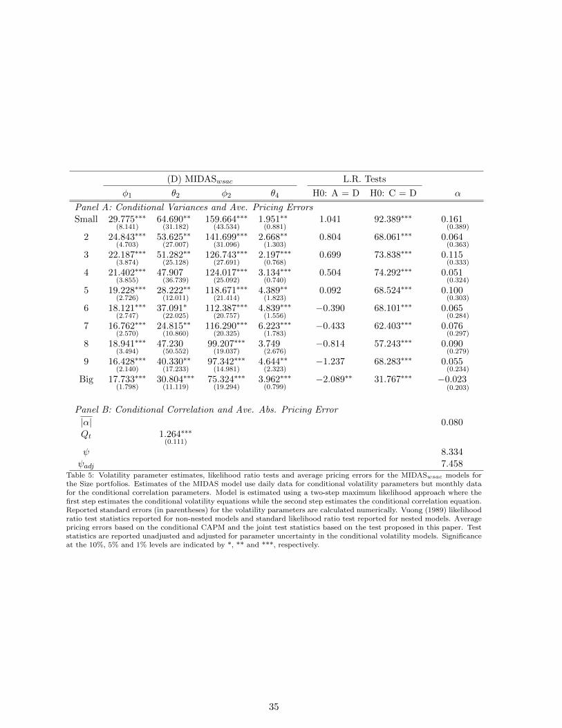
(D) MIDASwsac L.R. Tests

φ1 θ2 φ2 θ4 H0: A = D H0: C = D α

Panel A: Conditional Variances and Ave. Pricing ErrorsSmall 29.775∗∗∗

(8.141)64.690∗∗

(31.182)159.664∗∗∗

(43.534)1.951∗∗

(0.881)1.041 92.389∗∗∗ 0.161

(0.389)

2 24.843∗∗∗(4.703)

53.625∗∗(27.007)

141.699∗∗∗(31.096)

2.668∗∗(1.303)

0.804 68.061∗∗∗ 0.064(0.363)

3 22.187∗∗∗(3.874)

51.282∗∗(25.128)

126.743∗∗∗(27.691)

2.197∗∗∗(0.768)

0.699 73.838∗∗∗ 0.115(0.333)

4 21.402∗∗∗(3.855)

47.907(36.739)

124.017∗∗∗(25.092)

3.134∗∗∗(0.740)

0.504 74.292∗∗∗ 0.051(0.324)

5 19.228∗∗∗(2.726)

28.222∗∗(12.011)

118.671∗∗∗(21.414)

4.389∗∗(1.823)

0.092 68.524∗∗∗ 0.100(0.303)

6 18.121∗∗∗(2.747)

37.091∗(22.025)

112.387∗∗∗(20.757)

4.839∗∗∗(1.556)

−0.390 68.101∗∗∗ 0.065(0.284)

7 16.762∗∗∗(2.570)

24.815∗∗(10.860)

116.290∗∗∗(20.325)

6.223∗∗∗(1.783)

−0.433 62.403∗∗∗ 0.076(0.297)

8 18.941∗∗∗(3.494)

47.230(50.552)

99.207∗∗∗(19.037)

3.749(2.676)

−0.814 57.243∗∗∗ 0.090(0.279)

9 16.428∗∗∗(2.140)

40.330∗∗(17.233)

97.342∗∗∗(14.981)

4.644∗∗(2.323)

−1.237 68.283∗∗∗ 0.055(0.234)

Big 17.733∗∗∗(1.798)

30.804∗∗∗(11.119)

75.324∗∗∗(19.294)

3.962∗∗∗(0.799)

−2.089∗∗ 31.767∗∗∗ −0.023(0.203)

Panel B: Conditional Correlation and Ave. Abs. Pricing Error

|α| 0.080Qt 1.264∗∗∗

(0.111)

ψ 8.334ψadj 7.458

Table 5: Volatility parameter estimates, likelihood ratio tests and average pricing errors for the MIDASwsac models forthe Size portfolios. Estimates of the MIDAS model use daily data for conditional volatility parameters but monthly datafor the conditional correlation parameters. Model is estimated using a two-step maximum likelihood approach where thefirst step estimates the conditional volatility equations while the second step estimates the conditional correlation equation.Reported standard errors (in parentheses) for the volatility parameters are calculated numerically. Vuong (1989) likelihoodratio test statistics reported for non-nested models and standard likelihood ratio test reported for nested models. Averagepricing errors based on the conditional CAPM and the joint test statistics based on the test proposed in this paper. Teststatistics are reported unadjusted and adjusted for parameter uncertainty in the conditional volatility models. Significanceat the 10%, 5% and 1% levels are indicated by *, ** and ***, respectively.

35

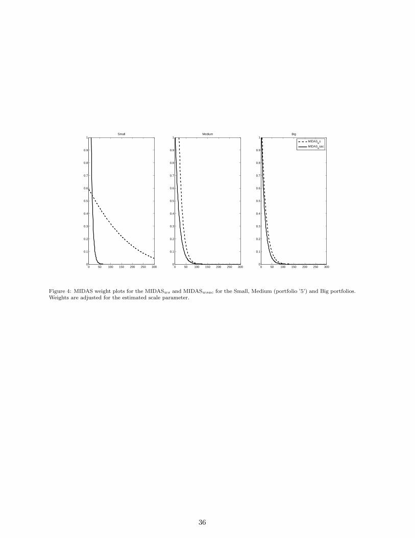
0 50 100 150 200 250 3000

0.1

0.2

0.3

0.4

0.5

0.6

0.7

0.8

0.9

1Small

0 50 100 150 200 250 3000

0.1

0.2

0.3

0.4

0.5

0.6

0.7

0.8

0.9

1Medium

0 50 100 150 200 250 3000

0.1

0.2

0.3

0.4

0.5

0.6

0.7

0.8

0.9

1Big

MIDAS

ws

MIDASw

sac

Figure 4: MIDAS weight plots for the MIDASws and MIDASwsac for the Small, Medium (portfolio ’5’) and Big portfolios.Weights are adjusted for the estimated scale parameter.

36

Small 2 3 4 5 6 7 8 9 Big

-0.1

0

0.1

0.2

0.3

0.4

0.5Full Sample

Small 2 3 4 5 6 7 8 9 Big

-0.1

0

0.1

0.2

0.3

0.4

0.51st Half

Small 2 3 4 5 6 7 8 9 Big

-0.1

0

0.1

0.2

0.3

0.4

0.52nd Half

UnconditionalDCC

MIDASw

sac

Figure 5: Average pricing error plots of the unconditional and conditional CAPM for the Size Portfolios for the full, firsthalf and second half of the sample. Conditional CAPM plots are based on the DCC and MIDASwsac conditional volatilitymodels.

37

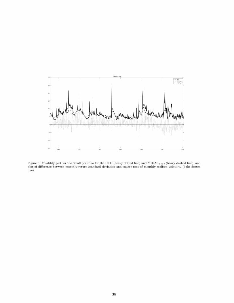
1966 1974 1983 1991 1999 2008 2016-15

-10

-5

0

5

10

15

20

25

30Volatility Plot

DCCMIDAS

wsac

(r2)1/2-RV1/2

Figure 6: Volatility plot for the Small portfolio for the DCC (heavy dotted line) and MIDASwsac (heavy dashed line), andplot of difference between monthly return standard deviation and square-root of monthly realised volatility (light dottedline).

38

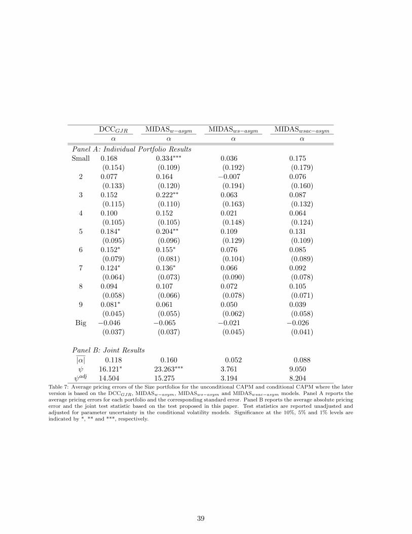
DCCGJR MIDASw−asym MIDASws−asym MIDASwsac−asymα α α α

Panel A: Individual Portfolio ResultsSmall 0.168 0.334∗∗∗ 0.036 0.175

(0.154) (0.109) (0.192) (0.179)2 0.077 0.164 −0.007 0.076

(0.133) (0.120) (0.194) (0.160)3 0.152 0.222∗∗ 0.063 0.087

(0.115) (0.110) (0.163) (0.132)4 0.100 0.152 0.021 0.064

(0.105) (0.105) (0.148) (0.124)5 0.184∗ 0.204∗∗ 0.109 0.131

(0.095) (0.096) (0.129) (0.109)6 0.152∗ 0.155∗ 0.076 0.085

(0.079) (0.081) (0.104) (0.089)7 0.124∗ 0.136∗ 0.066 0.092

(0.064) (0.073) (0.090) (0.078)8 0.094 0.107 0.072 0.105

(0.058) (0.066) (0.078) (0.071)9 0.081∗ 0.061 0.050 0.039

(0.045) (0.055) (0.062) (0.058)Big −0.046 −0.065 −0.021 −0.026

(0.037) (0.037) (0.045) (0.041)

Panel B: Joint Results

|α| 0.118 0.160 0.052 0.088ψ 16.121∗ 23.263∗∗∗ 3.761 9.050ψadj 14.504 15.275 3.194 8.204

Table 7: Average pricing errors of the Size portfolios for the unconditional CAPM and conditional CAPM where the laterversion is based on the DCCGJR, MIDASw−asym, MIDASws−asym and MIDASwsac−asym models. Panel A reports theaverage pricing errors for each portfolio and the corresponding standard error. Panel B reports the average absolute pricingerror and the joint test statistic based on the test proposed in this paper. Test statistics are reported unadjusted andadjusted for parameter uncertainty in the conditional volatility models. Significance at the 10%, 5% and 1% levels areindicated by *, ** and ***, respectively.

39

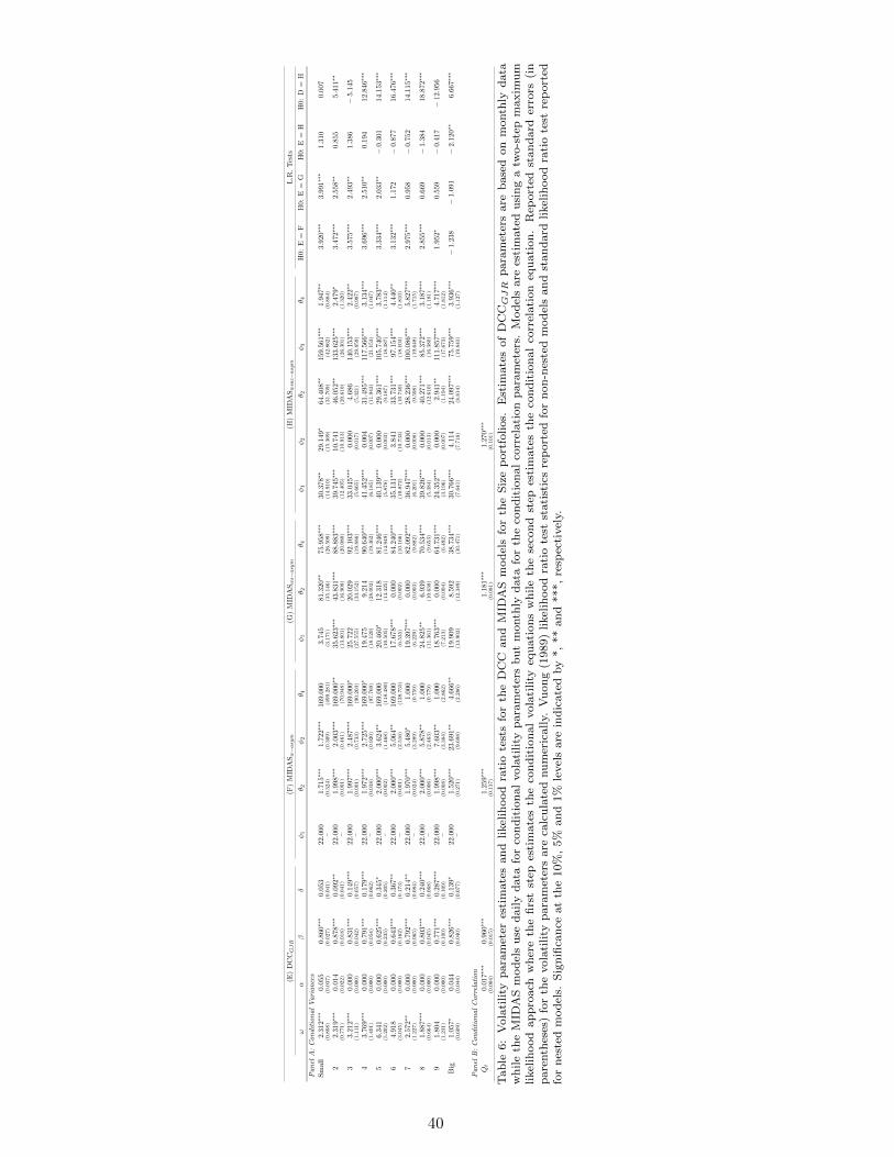
(E)

DC

CGJR

(F)

MID

ASw−asym

(G)

MID

ASws−asym

(H)

MID

ASwsac−asym

L.R

.T

ests

ωα

βδ

φ1

θ 2φ

2θ 4

φ1

θ 2θ 4

φ1

φ2

θ 2φ

3θ 4

H0:

E=

FH

0:

E=

GH

0:

E=

HH

0:

D=

H

Panel

A:ConditionalVariances

Sm

all

2.31

2∗∗∗

(0.8

08)

0.05

5(0.0

37)

0.8

60∗∗∗

(0.0

27)

0.05

3(0.0

41)

22.0

00−

1.7

15∗∗∗

(0.3

24)

1.72

2∗∗∗

(0.3

09)

169.0

00(4

99.2

81)

3.74

5(3.1

71)

81.3

20∗∗

(35.1

46)

75.9

58∗∗∗

(26.5

09)

30.3

78∗∗

(14.9

10)

29.1

49∗

(15.3

69)

64.4

08∗∗

(31.7

69)

159.

561∗∗∗

(42.8

62)

1.9

47∗∗

(0.8

84)

3.9

20∗∗∗

3.991∗∗∗

1.310

0.0

07

22.

319∗∗∗

(0.7

71)

0.0

14(0.0

22)

0.8

78∗∗∗

(0.0

18)

0.09

2∗∗

(0.0

41)

22.0

00−

1.99

8∗∗∗

(0.0

01)

2.0

03∗∗∗

(0.4

61)

169.0

00∗∗

(70.9

48)

35.6

23∗∗∗

(13.8

01)

43.8

31∗∗∗

(16.9

08)

88.

883∗∗∗

(20.0

80)

39.7

45∗∗∗

(12.4

05)

10.

741

(10.9

13)

46.0

52∗∗

(20.6

10)

133.6

25∗∗∗

(26.3

01)

2.479∗

(1.3

20)

3.4

72∗∗∗

2.5

58∗∗

0.855

5.4

11∗∗

33.

212∗∗∗

(1.1

11)

0.0

00(0.0

00)

0.83

1∗∗∗

(0.0

42)

0.1

49∗∗∗

(0.0

57)

22.0

00−

1.99

7∗∗∗

(0.0

01)

2.4

87∗∗∗

(0.7

33)

169.0

00∗

(90.2

03)

25.7

22(2

7.5

55)

20.0

29

(33.1

52)

92.1

03∗∗∗

(19.8

86)

33.0

45∗∗∗

(5.6

65)

0.00

0(0.0

17)

4.686

(5.3

21)

140.1

53∗∗∗

(29.8

59)

2.422∗∗

(0.9

87)

3.5

75∗∗∗

2.4

93∗∗

1.386

−5.

145

43.

769∗∗∗

(1.4

01)

0.0

00(0.0

00)

0.79

1∗∗∗

(0.0

54)

0.1

79∗∗∗

(0.0

62)

22.0

00−

1.9

72∗∗∗

(0.0

18)

2.7

25∗∗∗

(0.9

20)

169.

000∗

(97.7

69)

19.4

75(1

8.1

20)

9.21

4(2

8.0

03)

90.6

40∗∗∗

(19.3

62)

41.4

52∗∗∗

(6.1

85)

0.00

4(0.0

07)

31.4

95∗∗∗

(11.9

43)

117.5

66∗∗∗

(21.1

53)

3.134∗∗∗

(1.0

47)

3.696∗∗∗

2.5

10∗∗

0.1

94

12.8

46∗∗∗

56.

341

(5.2

02)

0.00

0(0.0

00)

0.62

5∗∗∗

(0.2

35)

0.3

45∗

(0.2

05)

22.0

00−

2.0

00∗∗∗

(0.0

02)

3.62

4∗∗

(1.4

68)

169.

000

(118.4

80)

20.4

60∗

(10.5

05)

12.3

18(1

4.4

25)

81.2

46∗∗∗

(14.9

49)

40.1

39∗∗∗

(5.8

78)

0.00

0(0.0

03)

29.3

61∗∗∗

(9.1

87)

105.7

40∗∗∗

(18.3

87)

3.783∗∗∗

(1.1

14)

3.334∗∗∗

2.0

33∗∗

−0.3

01

14.

153∗∗∗

64.

918

(3.0

45)

0.00

0(0.0

00)

0.6

43∗∗∗

(0.1

62)

0.3

67∗∗

(0.1

73)

22.0

00−

2.0

00∗∗∗

(0.0

01)

5.06

4∗∗

(2.5

16)

169.

000

(128.7

55)

17.6

78∗∗∗

(6.5

35)

0.000

(0.0

02)

84.2

40∗∗∗

(10.1

66)

35.1

31∗∗∗

(10.8

72)

3.8

41(1

0.7

33)

33.

731∗∗∗

(10.7

40)

97.

154∗∗∗

(18.1

03)

4.4

40∗∗

(1.8

10)

3.132∗∗∗

1.1

72

−0.8

77

16.

476∗∗∗

72.

572∗∗

(1.2

27)

0.00

0(0.0

00)

0.7

92∗∗∗

(0.0

65)

0.2

14∗∗

(0.0

84)

22.0

00−

1.9

70∗∗∗

(0.0

24)

5.48

0∗(3.2

89)

1.0

00(0.7

59)

19.3

97∗∗∗

(6.2

29)

0.00

0(0.0

03)

82.0

92∗∗∗

(9.8

82)

36.9

47∗∗∗

(6.2

01)

0.0

00

(0.0

08)

28.2

36∗∗∗

(9.5

98)

100.

086∗∗∗

(19.6

48)

5.8

27∗∗∗

(1.7

15)

2.975∗∗∗

0.958

−0.

752

14.1

15∗∗∗

81.

887∗∗∗

(0.6

64)

0.00

0(0.0

00)

0.8

03∗∗∗

(0.0

45)

0.24

0∗∗∗

(0.0

68)

22.0

00−

2.00

0∗∗∗

(0.0

06)

5.87

8∗∗

(2.4

63)

1.0

00(0.7

79)

24.8

25∗∗

(11.3

61)

6.9

39(1

0.6

38)

70.5

34∗∗∗

(9.6

53)

39.8

26∗∗∗

(5.3

84)

0.0

00(0.0

13)

40.2

71∗∗∗

(12.6

10)

85.

372∗∗∗

(16.3

80)

3.1

87∗∗∗

(1.1

81)

2.855∗∗∗

0.669

−1.

384

18.8

72∗∗∗

91.

804

(1.2

31)

0.0

00(0.0

00)

0.7

71∗∗∗

(0.1

00)

0.28

7∗∗∗

(0.1

09)

22.0

00−

1.99

8∗∗∗

(0.0

08)

7.6

03∗∗

(3.3

84)

1.0

00(2.8

62)

18.7

63∗∗∗

(7.2

13)

0.0

00(0.0

04)

64.

731∗∗∗

(6.4

92)

24.3

52∗∗∗

(3.1

96)

0.0

00(0.0

07)

2.94

1∗∗

(1.1

94)

111.8

57∗∗∗

(17.6

73)

4.7

17∗∗∗

(1.8

12)

1.9

52∗

0.559

−0.

417

−12.9

56

Big

1.05

7∗(0.6

09)

0.0

44(0.0

44)

0.82

6∗∗∗

(0.0

40)

0.13

9∗(0.0

77)

22.0

00−

1.52

0∗∗∗

(0.2

71)

23.6

91∗∗

(9.6

98)

4.6

66∗∗

(2.2

86)

19.9

09(1

3.9

03)

8.5

92(1

2.3

49)

38.7

34∗∗∗

(10.4

71)

30.7

66∗∗∗

(7.6

41)

4.11

4(7.7

18)

24.

097∗∗∗

(8.8

14)

75.7

59∗∗∗

(19.8

41)

3.936∗∗∗

(1.1

27)

−1.2

38

−1.0

91

−2.

120∗∗

6.6

67∗∗∗

Panel

B:ConditionalCorrelation

Qt

0.0

17∗∗∗

(0.0

04)

0.96

0∗∗∗

(0.0

15)

1.25

9∗∗∗

(0.1

17)

1.1

81∗∗∗

(0.0

81)

1.27

0∗∗∗

(0.1

01)

Tab

le6:

Vola

tility

para

met

eres

tim

ate

san

dlikel

ihood

rati

ote

sts

for

the

DC

Can

dM

IDA

Sm

od

els

for

the

Siz

ep

ort

folios.

Est

imate

sof

DC

CGJR

para

met

ers

are

base

don

month

lyd

ata

wh

ile

the

MID

AS

mod

els

use

daily

data

for

con

dit

ion

al

vola

tility

para

met

ers

bu

tm

onth

lyd

ata

for

the

con

dit

ion

al

corr

elati

on

para

met

ers.

Mod

els

are

esti

mate

du

sin

ga

two-s

tep

maxim

um

likel

ihood

ap

pro

ach

wh

ere

the

firs

tst

epes

tim

ate

sth

eco

nd

itio

nal

vola

tility

equ

ati

on

sw

hile

the

seco

nd

step

esti

mate

sth

eco

nd

itio

nal

corr

elati

on

equ

ati

on

.R

eport

edst

an

dard

erro

rs(i

np

are

nth

eses

)fo

rth

evola

tility

para

met

ers

are

calc

ula

ted

nu

mer

ically.

Vu

on

g(1

989)

likel

ihood

rati

ote

stst

ati

stic

sre

port

edfo

rn

on

-nes

ted

mod

els

an

dst

an

dard

likel

ihood

rati

ote

stre

port

edfo

rn

este

dm

od

els.

Sig

nifi

can

ceat

the

10%

,5%

an

d1%

level

sare

ind

icate

dby

*,

**

an

d***,

resp

ecti

vel

y.

40

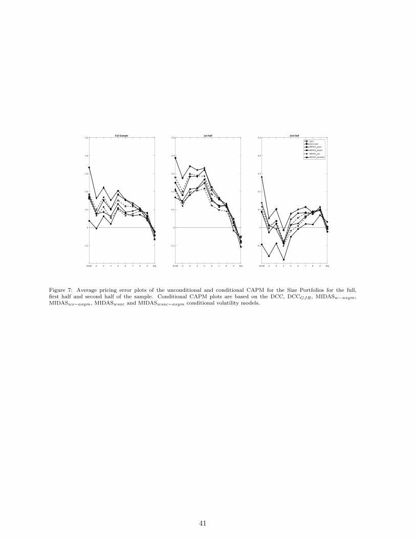
Small 2 3 4 5 6 7 8 9 Big

-0.1

0

0.1

0.2

0.3

0.4

0.5Full Sample

Small 2 3 4 5 6 7 8 9 Big

-0.1

0

0.1

0.2

0.3

0.4

0.51st Half

Small 2 3 4 5 6 7 8 9 Big

-0.1

0

0.1

0.2

0.3

0.4

0.52nd Half

DCCDCC-GJR

MIDASw

asym

MIDASw

sasym

MIDASw

sac

MIDASw

sacasym

Figure 7: Average pricing error plots of the unconditional and conditional CAPM for the Size Portfolios for the full,first half and second half of the sample. Conditional CAPM plots are based on the DCC, DCCGJR, MIDASw−asym,MIDASws−asym, MIDASwsac and MIDASwsac−asym conditional volatility models.

41

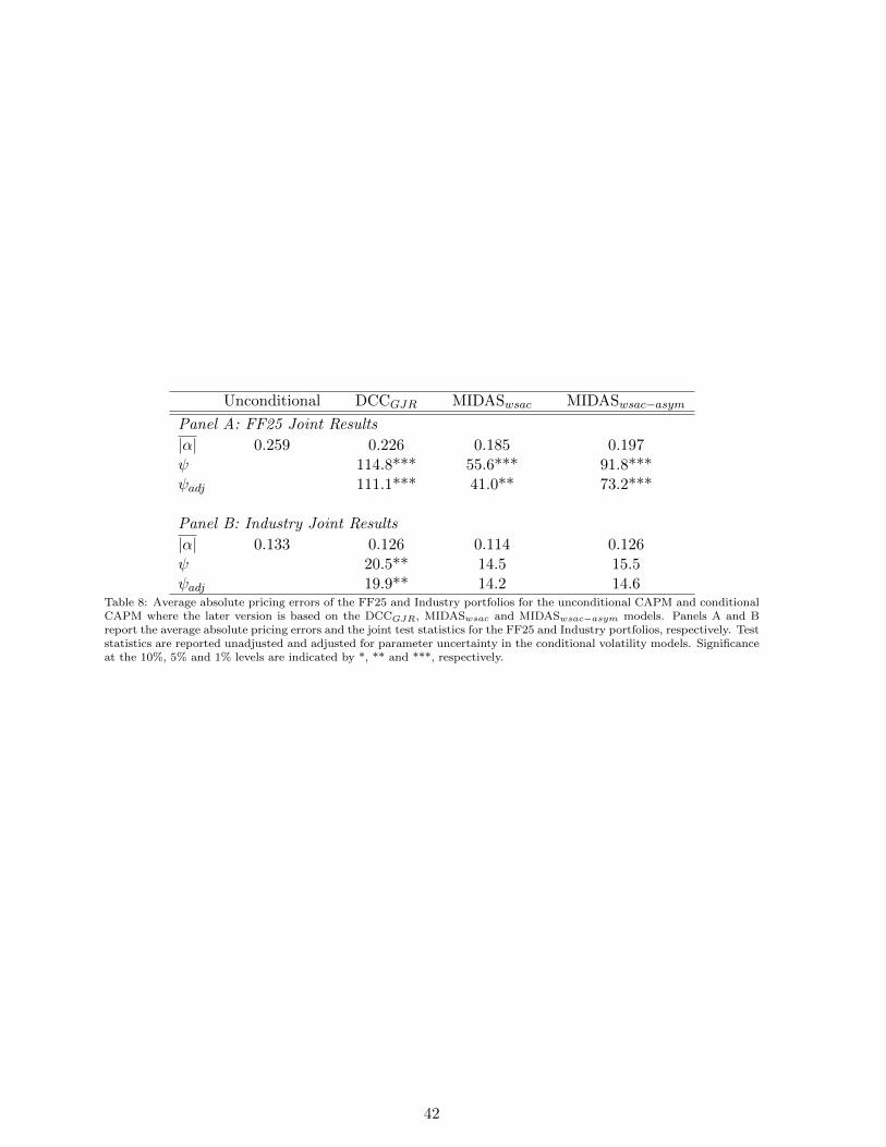
Unconditional DCCGJR MIDASwsac MIDASwsac−asym

Panel A: FF25 Joint Results

|α| 0.259 0.226 0.185 0.197ψ 114.8*** 55.6*** 91.8***ψadj 111.1*** 41.0** 73.2***

Panel B: Industry Joint Results

|α| 0.133 0.126 0.114 0.126ψ 20.5** 14.5 15.5ψadj 19.9** 14.2 14.6

Table 8: Average absolute pricing errors of the FF25 and Industry portfolios for the unconditional CAPM and conditionalCAPM where the later version is based on the DCCGJR, MIDASwsac and MIDASwsac−asym models. Panels A and Breport the average absolute pricing errors and the joint test statistics for the FF25 and Industry portfolios, respectively. Teststatistics are reported unadjusted and adjusted for parameter uncertainty in the conditional volatility models. Significanceat the 10%, 5% and 1% levels are indicated by *, ** and ***, respectively.

42