BANK OF GREECE

EUROSYSTEM

Working Paper

Economic Research Department

BANK OF GREECE

EUROSYSTEM

Special Studies Division21, E. Venizelos Avenue

Tel.:+30 210 320 3610Fax:+30 210 320 2432www.bankofgreece.gr

GR - 102 50, Athens

WORKINKPAPERWORKINKPAPERWORKINKPAPERWORKINKPAPERISSN: 1109-6691

A conditional CAPM; implications for the estimation of

systematic risk

Alexandros E. MilionisDimitra K. Patsouri

13MAY 2011WORKINKPAPERWORKINKPAPERWORKINKPAPERWORKINKPAPERWORKINKPAPER

1

BANK OF GREECE Economic Research Department – Special Studies Division 21, Ε. Venizelos Avenue GR-102 50 Athens Τel: +30210-320 3610 Fax: +30210-320 2432 www.bankofgreece.gr Printed in Athens, Greece at the Bank of Greece Printing Works. All rights reserved. Reproduction for educational and non-commercial purposes is permitted provided that the source is acknowledged. ISSN 1109-6691

A CONDITIONAL CAPM; IMPLICATIONS FOR THE ESTIMATION OF SYSTEMATIC RISK

Alexandros E. Milionis Bank of Greece and University of the Aegean

Dimitra K. Patsouri

University of Athens

Abstract The purpose of this paper is to examine: (i) whether or not, the residuals of the Market Model are conditionally heteroscedastic; (ii) whether or not, there exists an intervalling effect in conditional heteroscedasticity in the residuals of the Market Model; (iii) the effect of conditional heteroscedasticity on the estimation of systematic risk.; as well as to propose a simple data driven conditional CAPM. To this end daily closing price of stocks traded at the Athens Stock Exchange are used. Empirical evidence is provided for the existence of: (a) conditional heteroscedasticity in MM residuals; (b) a pronounced intervalling effect on ARCH in MM residuals; (c) GARCH in mean type of conditional heteroscedasticity for the majority of cases where ARCH was present in MM residuals. These findings in terms of theory are conducive to a conditional CAPM, which takes into account the effect of conditional variance on expected returns, rather than the standard CAPM. Furthermore, in terms of practical implications these findings may lead to better estimates of systematic risk Keywords: Conditional Capital Asset Pricing Model, Market Model, Conditional Volatility, Systematic Risk, Intervalling Effect, Athens Stock Exchange.

JEL Classification: C10, G10, G11, G12, G32

Ackowledgements: The authors are grateful to H. Gibson for helpful comments. The views expressed in the paper are those of the authors and do not necessarily reflect those of the Bank of Greece.

Correspondence: Alexandros E. Milionis Bank of Greece, Department of Statistics 21 E. Venizelos Avenue, Athens, GR 102 50 Tel.: +30-210 3203855, e-mail: amilionis@bankofgreece.gr

1. Introduction

Among the most fundamental issues in finance is the relation between risk and

return. There is little doubt that thus far the Capital Asset Pricing Model (CAPM) of

Sharp (1964), Lintner (1965) and Black (1972) has played a very important role, as it

describes how investors react to risk and value risky assets. More specifically CAPM

expresses the expected return of the risky asset j E(Rj) as follows:

)]([)( fmjfj RRERRE −+= β

Where:

Rf is the return on the risk free asset;

Rm is the return on the whole economy, usually approximated by a composite market

index;

βj is the so-called beta or systematic risk coefficient of asset j.

As is apparent, according to the CAPM, the expected return of asset j is a linear

function of its corresponding beta and presumably this one-dimensional expression for

risk suffices to describe the cross section of expected returns. There is a voluminous

literature on the ability of the CAPM to explain observed asset returns and there are

serious specification issues that have been raised regarding its ability to explain much.

For instance, Fama and French in a series of papers during the 90s (Fama and French

1992, 1993, 1996) found that the (standard) CAPM does not hold empirically. Fama and

French proposed the so-called Three Factor Model (TFM) which reflects the fact that two

classes of stocks (those with small capitalization and high book to market value) tend to

do better than the market as a whole. TFM has gained recognition in financial

management and many studies have shown that the majority of actively managed mutual

funds underperform broad indices based on Fama and French’s three factors, if classified

properly. However, the success of the TFM spurred a considerable debate in the literature

and the main reason is that the extra two factors used by Fama and French are just returns

on portfolios formed on the same characteristics which lack a clear economic relationship

with systematic risk. At the same time, numerous attempts have been made to explore the

nature of the anomalies associated with the standard CAPM and correct them. Breen et al

5

(1989) showed that betas in the CAPM framework are not time-invariant but rather vary

over the business cycles, as also shown by Chen (1991). Jaganathan and Wang (1996)

have developed a conditional version of the CAPM in which it is assumed that the CAPM

holds in a conditional sense allowing beta and the market risk premium to vary over time.

A main problem with the conditional CAPMs in general is the choice of conditioning

variables and the lack of theory about how to form the relationship between the betas and

the conditioning variables.

The present work using the standard static CAPM as a starting point tries to look at

the context of a conditional CAPM for a specific simple conditional type of CAPM where

the conditioning is data driven, derived by an examination of the residuals of the so-

called market model. Such a model may lead to more accurate estimates of systematic

risk. The rest of the paper is structured as follows: the methodological approach is

explained in section 2; the empirical results are presented and commented upon in section

3; section 4 summarizes and concludes the paper.

2. Data and methodological approach

The data are daily closing prices of all stocks traded on the Athens Stock Exchange

for the period from 1/10/1999 to 30/9/2004 and were provided by the Athens Stock

Exchange (ASE). From May 31 2001, the ASE joined the mature financial markets

according to the classification of Morgan Stanley Capital International. Until that date,

the ASE belonged to the European Emerging Markets. Its current total capitalization is

about 70 million euro. Further details about the ASE are given in many papers (see for

instance Milionis and Papanagiotou, 2009). The Athens General Index is used as the

market index. Returns are expressed as logarithmic differences of (adjusted) price

relatives.

It must first be noted that methodologically the CAPM is a general equilibrium

model; hence, both the return of the each time particular asset and the market return are

expected future returns, while the relevant coefficient of systematic risk is the future beta

of the each time particular asset. Unfortunately data for expected future returns do not

exist. What is feasible is to perform an ex post analysis of ex ante expected returns. In

6

order to replace ex-ante with ex-post realized returns, it has to be assumed that

expectations are on average correct and therefore actual events can be considered as

proxies for expectations. Hence, the common approach for the estimation of the standard

betas is to use the so-called Market Model (henceforth MM) and OLS estimators. In that

way, a beta is estimated as the slope coefficient in the regression:

Rj = αj + βjRm + uj

Where uj is the stochastic disturbance and αj is a constant. It is noticeable that the the risk

free rate is not included in the MM. For realistic changes in the value of the risk free rate,

there is very little difference in the estimated beta values.

Not taking into consideration phenomena related to market microstructure, one

would expect that beta estimates would be invariant to changes in the length of the

differencing interval over which index and security returns are calculated. However, a

plethora of empirical findings suggest that this is not the case. Indeed, it has been found

that beta estimates change systematically as the differencing interval over which they are

estimated is lengthened (see for instance Corhay, 1991, Cohen et al. 1983a, Scholes and

Williams 1977, Dimson, 1979). This phenomenon, known as “intervalling effect”, results

in a biased beta estimate and consequently in an incorrect assessment of a security’s risk.

The main reason for this bias is friction in the trading process and the price adjustment

delays entailed (Cohen et al., 1983b). The magnitude of the bias decreases as the

differencing interval over which returns are calculated (henceforth denoted by l) is

increased and it has been proved that (Fung et al., 1985):

jN

lp ββ =∞→∞→

))(ˆ lim (lim olsjl

(1)

where N is the sample size, is the OLS estimator of beta corresponding to

differencing interval l and is the true value of the market risk for security j.

)(ˆ olsj lβ

jβ

Based on what eq. (1) implies in terms of the behaviour of betas as the differencing

interval increases without bound, Cohen et al. (1983a) have suggested a methodology

leading to unbiased estimates of betas, the so-called asymptotic betas. This methodology

has been adopted by several other researchers.

7

The methodology described above is based exclusively on OLS estimates.

Although not explicitly stated in the finance textbooks, it must be noted at this point that

among the assumptions for the validity of the MM is that the residual variance should be

constant both in the unconditional and conditional sense. Theoretical considerations (e.g.

Bollerslev et al., 1992; Nelson 1992) as well as empirical evidence offer support for a

kind an “intervalling effect” on autoregressive conditional heteroscedasticity (henceforth

ARCH) in stock returns and exchange rates (e.g. Brailsford, 1995; Baillie and Bollerslev,

1989). Therefore, ARCH is expected and indeed has been found to be more pronounced

in higher frequency returns. In spite of its importance for the accuracy of the estimates of

systematic risk, such an investigation has not been undertaken in the residuals of the

classical MM thus far. In the next section the possibility of an intervalling effect in MM

residuals is explored and evidence is provided for the existence of such an effect.

Moreover, the character of this effect is examined and further analyzed.

More specifically, the MM will be estimated using differencing intervals from one

up to thirty days. It is noted that for l >1, estimates of beta corresponding to the same l

but estimated using a different starting day may be different (Corhay, 1992). To take into

account, this effect for differencing intervals of length l >1, l estimates of beta will be

obtained, each corresponding to a different starting day within the differencing interval l.

The final estimate of beta corresponding to differencing interval l will be the average of

these l estimates (see Corhay, 1992 for a detailed discussion on that point). A Ljung-Box

test for autocorrelation in the squared residuals of the market model will be performed for

each case. For every case that the Ljung–Box test results are significant, i.e. there exists

autoregressive conditional heteroscedasticity in the residuals of the MM, the following

models of conditional volatility will be estimated:

(a) GARCH(1,1)

itmtiit uRaR ++= β

211

2110

2−− ++= ttt u σβαασ

(b) EGARCH(1,1)

itmtiit uRaR ++= β

8

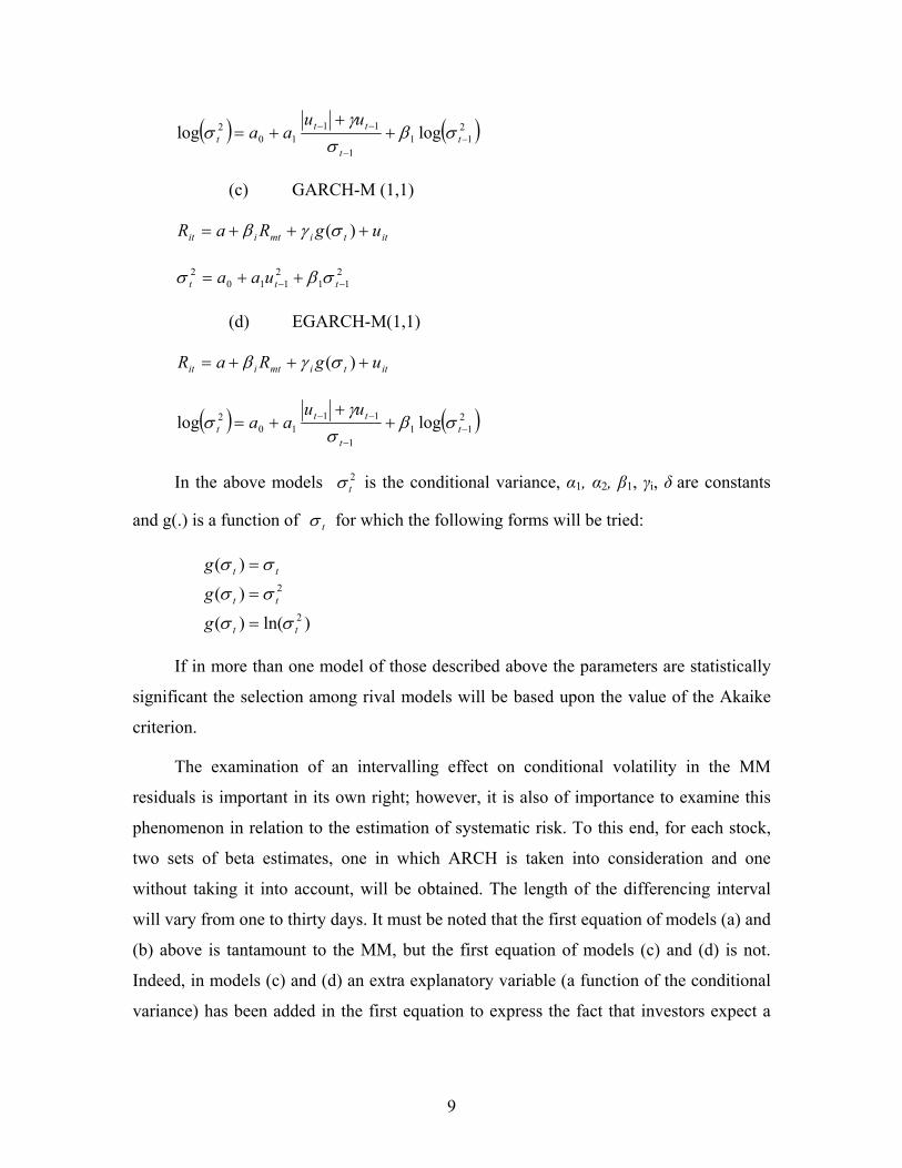
( ) ( )211

1

1110

2 loglog −−

−− ++

+= tt

ttt

uuaa σβ

σγ

σ

(c) GARCH-M (1,1)

ittimtiit ugRaR +++= )(σγβ

211

2110

2−− ++= ttt uaa σβσ

(d) EGARCH-M(1,1)

ittimtiit ugRaR +++= )(σγβ

( ) ( )211

1

1110

2 loglog −−

−− ++

+= tt

ttt

uuaa σβ

σγ

σ

In the above models is the conditional variance, α2tσ 1, α2, β1, γi, δ are constants

and g(.) is a function of for which the following forms will be tried: tσ

)ln()(

)(

)(

2

2

tt

tt

tt

g

g

g

σσ

σσ

σσ

=

=

=

If in more than one model of those described above the parameters are statistically

significant the selection among rival models will be based upon the value of the Akaike

criterion.

The examination of an intervalling effect on conditional volatility in the MM

residuals is important in its own right; however, it is also of importance to examine this

phenomenon in relation to the estimation of systematic risk. To this end, for each stock,

two sets of beta estimates, one in which ARCH is taken into consideration and one

without taking it into account, will be obtained. The length of the differencing interval

will vary from one to thirty days. It must be noted that the first equation of models (a) and

(b) above is tantamount to the MM, but the first equation of models (c) and (d) is not.

Indeed, in models (c) and (d) an extra explanatory variable (a function of the conditional

variance) has been added in the first equation to express the fact that investors expect a

9

higher return for the extra uncertainty due to the non-constancy of the conditional

variance.

3. Results and discussion

The results regarding the dependence of conditional volatility in the MM residuals

on the length of the differencing interval are presented in the form of a graph in Figure 1.

More specifically, Figure 1 shows the percentage (%) of cases for which the Ljung-Box

test in the square of the residuals of the MM rejects the null hypothesis of no

autocorrelation (at the 5% significance level) as a function of the length of the

differencing interval. As is evident from the results of Figure 1, autoregressive

conditional heteroscedasticity is found in 97.4% of the cases for l = 1. This percentage

decreases rapidly being less than 7% for differencing intervals greater than about 20-22

days. Overall these results are suggestive of the existence of a strong intervalling effect in

MM residuals.

Furthermore, the extent to which autoregressive conditional heteroscedasticity

appears in the form a (E)GARCH in mean type of model will be examined (models (c) or

(d) in the previous section). This is important since in these cases the CAPM is

misspecified and an extra term, related to the conditional variance, must be included in

the right hand side of the MM. Consequently, given that the corresponding partial

regression coefficient is expected to be positive (see Milionis and Moschos, 2000 for a

detailed discussion on that point), with GARCH in mean conditional volatility beta

estimates are expected to be reduced. Owing to the existence of this extra term, as

explained above, βj can no longer play the role of the sole risk factor on such occasions

and will be called the market beta hereafter.

Figure 2 shows the percentage (%) of cases for which ARCH is of GARCH in

mean type in the MM residuals, out of both the total number of cases (triangles) and the

number of cases with ARCH (squares). From Figure 2, at first it is evident that, as is the

case with conditional volatility in the MM residuals in general, there is a pronounced

intervalling effect in the GARCH in mean type of conditional volatility. It is also noted

that, despite its fluctuations, GARCH in mean type of volatility as a percentage of the

10

total cases with ARCH does not exhibit any conspicuous intervalling effect and for most

differencing intervals represents the majority of ARCH cases.

It must be clarified that the above findings do not imply a rejection of the CAPM.

Indeed, as noted in the previous section, the CAPM assumes a constant variance in the

deviations from equilibrium. The previous empirical results indicate that this condition

does not hold for the majority of cases. Hence, models (c) and (d) must be seen as

generalizations of the CAPM under more general conditions i.e. allowing for the presence

of (E)GARCH in mean conditional heteroscedasticity. It must also be noted that even

using models (a) and (b), where no extra term is added to the MM model, the estimation

of beta using these models is more efficient than the corresponding OLS estimate.

It is of much importance to investigate the alleged influence of conditional

volatility on the estimation of systematic risk. Figure 3 shows the variation of average

OLS beta and average market beta with the length of the differencing interval. From the

character of this variation, as shown in Figure 3, several interesting comments can be

made. At first it is noted that the value of average betas is greater than one in all cases.

This is not surprising as betas of individual stocks are not weighted by the corresponding

capitalization values for the calculation of the average beta. Further, average beta (and

average market beta for the GARCH cases) increases with the length of the differencing

interval with both OLS and GARCH estimation, confirming the existence of an

intervalling effect in betas. However, estimates of (market) betas which take into

consideration autoregressive conditional heteroscedasticity are always lower than the

corresponding (for the same differencing interval) betas estimated purely with OLS. This

difference takes its maximum values for the shortest differencing intervals (one to four

days) confirming the point made previously.

Further insight about the magnitude of the deviation of beta estimates using the two

methods is provided in Figure 4. This figure shows the variation of the value of the mean

absolute percentage error (MAPE) across the differencing interval. This statistic is

calculated by the formula:

11

∑=

−⎟⎟⎟

⎠

⎞

⎜⎜⎜

⎝

⎛⋅

−=

J

jGARCHj

GARCHj

OLSj

OLSGARCH JMAPE

1100ˆ

ˆˆ1β

ββ

where J is the total number of securities.

As is evident from Figure 4, as a result of the intervalling effect on conditional

volatility in the MM residuals, the difference in the beta estimates due to the method of

estimation is much more substantial for the shorter differencing intervals, (exceeding

15% for differencing intervals of 2 and 3 days) as compared to the longest differencing

intervals where this difference is only of the order of 2% to 3%.

4. Summary and conclusions

Despite the criticism of the standard CAPM, as described in the introduction, for a

variety of reasons (see for instance Jagatnathan and Wang, 1996, Elton et al., 2007) betas

are still the most widely used measure of systematic risk by analysts and financial

managers.

In this work empirical evidence is provided for the existence of: (a) conditional

heteroscedasticity in MM residuals; (b) a pronounced intervalling effect on ARCH in

MM residuals; and (c) GARCH in mean type of conditional heteroscedasticity for the

majority of cases where ARCH was present in MM residuals.

As a consequence of (a), the use of simple OLS for the estimation of betas is not

justified. As a consequence of (b), autoregressive conditional heteroscedasticity affects

unevenly the OLS estimates of betas. As a consequence of (c), an extra term related to the

conditional variance must be added to the right hand side of CAPM. This simply reflects

the fact that the variance of returns is not constant in the conditional sense, as implied in

the standard CAPM. It is important to mention that the development of autoregressive

conditional heteroscedasticity models had not been developed when the CAPM was

introduced; hence, given the evidence provided in this work, the CAPM should be

augmented to allow for autoregressive conditional heteroscedasticity. Under such

conditions a conditional type CAPM is more appropriate. The highest influence on OLS

12

beta estimates is for differencing intervals up to five days for which the corresponding

market beta estimates are lower by more than 13%. These findings may help towards

better estimation of systematic risk. Methods which have been developed for the

estimation of systematic risk based on data of such frequencies (e.g. the so-called inferred

asymptotic betas, see Cohen et al., 1983b) must necessarily take into account the

intervalling effect on ARCH in MM residuals. Hence, the approach followed in this work

provides a relatively simple way to improve the accuracy of systematic risk estimates.

13

References

Baillie, R. T., Bollerslev, T. (1989), “The message in daily exchange rates: a conditional variance tale”, Journal of Business and Economic Statistics Vol. 7, pp. 297-305.

Black, F. (1972) “Capital market equilibrium with restricted borrowing, “Journal of Business, Vol. 45, pp. 444-455.

Bollerslev, T., Chou R. Y., Kroner, K. F. (1992), “ARCH modelling in Finance: a review of theory and empirical evidence”, Journal of Econometrics, Vol. 52, pp. 5-29.

Brailsford, T. J. (1995), “An empirical test of the effect of the return interval on conditional volatility”, Applied Economics Letters, Vol. 2, pp. 156-158.

Breen, W. J. Glosten, L. R. and Jagannathan, R. (1989), “Economic significance of predictable variations in stock index returns”, Journal of Finance, Vol. 44, pp. 1177-1190.

Chen, N. F. (1991), “Financial investment opportunities and the macroeconomy”, Journal of Finance, Vol. 46, pp. 529-554.

Cohen, K., Hawawini, G., Maier, S., Scwartz, R., Whitecomb, D. (1983a), “Estimating and adjusting for the intervalling effect bias in beta”, Management Science, Vol. 29 No 1, pp.135-148.

Cohen, K., Hawawini, G., Maier, S., Scwartz, R., Whitecomb, D. (1983b), “Friction in the trading process and the estimation of systematic risk”, Journal of Financial Economics, Vol. 12, pp. 263-278.

Corhay, A. (1992), “The intervalling effect bias in beta: a note”, Journal of Banking and Finance, Vol. 16, pp. 61-73.

Dimson, E. (1979), “Risk measurement when shares are subject to infrequent trading”, Journal of Financial Economics, Vol. 7, pp. 197-226.

Elton, E., M. Gruber, S. Brown, Goetzmann, W. (2007), Modern portfolio theory and investment analysis., 7th edition, Wiley, NY.

Fama, E. and French, K. R. (1992), “The cross section of expected stock returns”, Journal of Finance, Vol. 47, pp. 427-466.

Fama, E. and French, K. R. (1993), “Common risk factors in the returns on bonds and stocks”, Journal of Financial Economics, Vol. 33, pp. 3-56.

Fama, E. and French, K. R. (1996), Multifactor explanations of asset pricing anomalies, Journal of Finance, Vol 51, No. 1, pp.55-84.

Fung, W., Schwartz, R., Whitecomb, D. (1985), “Adjusting for the intervalling effect bias in beta. A test using Paris Boerse data” Journal of Banking and Finance, Vol. 9, pp. 443-460.

Jaganathan, R, and Wang, Z. (1996), “The conditional CAPM and the cross section of expected returns”, Journal of Finance, Vol. 51 No. 1, pp. 3-53.

14

Lintner, J. (1964) “The valuation of risk assets and the selection of risky investments in stock portfolio and capital budgets”, Review of Economics and Statistics, Vol. 47, pp. 13-37.

Milionis, A. E., Moschos, D. (2000), “On the Validity of the weak-form efficient markets hypothesis applied to the London Stock Exchange: comment”, Applied Economic Letters, Vol. 7, pp. 419-421

Milionis, A. E., Papanagiotou, E. (2009), “A study of the predictive performance of the moving average trading rule as applied to NYSE, the Athens Stock Exchange and the Vienna Stock Exchange: sensitivity analysis and implications for weak-form market efficiency testing”, Applied Financial Economics, Vol. 19, pp. 1171–1186

Nelson, D. B. (1992), “Filtering and forecasting with mis-specified ARCH models I: getting the right variance with the wrong model” Journal of Econometrics, Vol. 52, pp. 61-90.

Scholes, M., Williams, J. (1977), “Estimating beta from non-synchronous data” Journal of Financial Economics, Vol. 5, pp. 309-327.

Sharpe, W. F. (1964), “Capital assets prices: A theory of market equilibrium under conditions of risk”, Journal of Finance, Vol. 19, pp. 425-442.

15

Appendix

Figure 1. Percentage (%) of cases for which the Ljung-Box test in the square residuals of

the Market Model rejects the null hypothesis of no autocorrelation.

0102030405060708090

100

1 3 5 7 9 11 13 15 17 19 21 23 25 27 29

Differencing Interval (Days)

%

Figure 2. Percentage of GARCH in mean as a function of the differencing interval

0102030405060708090

100

1 3 5 7 9 11 13 15 17 19 21 23 25 27 29

Differencing Interval (Days)

%

% OF ALL CASES

% OF ARCH CASES

16

Figure 3. Variation of average beta with the length of the differencing interval

1

1.1

1.2

1.3

1.4

1.5

1.6

1 3 5 7 9 11 13 15 17 19 21 23 25 27 29

Differencing Interval (Days)

Ave

rage

bet

a

GARCHOLS

Figure 4. Variation of MAPE with the differencing interval

0

2

4

6

8

10

12

14

1 3 5 7 9 11 13 15 17 19 21 23 25 27 29

Differencing Interval (Days)

Val

ue o

f MAP

E (%

)

16

17

18

BANK OF GREECE WORKING PAPERS 116. Tagkalakis, A., “Fiscal Policy and Financial Market Movements”, July 2010.

117. Brissimis, N. S., G. Hondroyiannis, C. Papazoglou, N. T Tsaveas and M. A. Vasardani, “Current Account Determinants and External Sustainability in Periods of Structural Change”, September 2010.

118. Louzis P. D., A. T. Vouldis, and V. L. Metaxas, “Macroeconomic and Bank-Specific Determinants of Non-Performing Loans in Greece: a Comparative Study of Mortgage, Business and Consumer Loan Portfolios”, September 2010.

119. Angelopoulos, K., G. Economides, and A. Philippopoulos, “What Is The Best Environmental Policy? Taxes, Permits and Rules Under Economic and Environmental Uncertainty”, October 2010.

120. Angelopoulos, K., S. Dimeli, A. Philippopoulos, and V. Vassilatos, “Rent-Seeking Competition From State Coffers In Greece: a Calibrated DSGE Model”, November 2010.

121. Du Caju, P.,G. Kátay, A. Lamo, D. Nicolitsas, and S. Poelhekke, “Inter-Industry Wage Differentials in EU Countries: What Do Cross-Country Time Varying Data Add to the Picture?”, December 2010.

122. Dellas H. and G. S. Tavlas, “The Fatal Flaw: The Revived Bretton-Woods system, Liquidity Creation, and Commodity-Price Bubbles”, January 2011.

123. Christopoulou R., and T. Kosma, “Skills and wage Inequality in Greece: Evidence from Matched Employer-Employee Data, 1995-2002”, February 2011.

124. Gibson, D. H., S. G. Hall, and G. S. Tavlas, “The Greek Financial Crisis: Growing Imbalances and Sovereign Spreads”, March 2011.

125. Louri, H. and G. Fotopoulos, “On the Geography of International Banking: the Role of Third-Country Effects”, March 2011.

126. Michaelides, P. G., A. T. Vouldis, E. G. Tsionas, “Returns to Scale, Productivity and Efficiency in Us Banking (1989-2000): The Neural Distance Function Revisited”, March 2011.

127. Gazopoulou, E. “Assessing the Impact of Terrorism on Travel Activity in Greece”, April 2011.

128. Athanasoglou, P. “The Role of Product Variety and Quality and of Domestic Supply in Foreign Trade”, April 2011.

129. Galuščắk, K., M. Keeney, D. Nicolitsas, F. Smets, P. Strzelecki and Matija Vodopivec, “The Determination of Wages of Newly Hired Employees: Survey Evidence on Internal Versus External Factors”, April 2011.

130. Kazanas, T., and. E. Tzavalis “Unveiling the Monetary Policy Rule In the Euro-Area”, May 2011.

19