Modeling VaR OF DAX INDEX USING GARCH MODEL · composite conditional mean and variance model using GARCH(1,1) model. We finally apply GARCH methodology to estimate VaR and compare

Prognostické práce, 6, 2014, č. 5 403

Modeling VaR OF DAX INDEX USING GARCH MODEL

Matej Štalmach1

Abstract

The Box-Jenkins time series analysis rests on important concept as stationarity and residuals

of ARMA models follows white noise. These concepts are insufficient for the analysis of

financial time series. The paper proposes main characteristics of volatility in financial time

series and general overview of most common models for time series modeling. This paper

also outlines characteristics of DAX and SAX index’s volatility and shows how to specify a

composite conditional mean and variance model using GARCH(1,1) model. We finally apply

GARCH methodology to estimate VaR and compare with other approach for DAX and SAX

indices. In general those indices might represent development and variability of business

sector in German and Slovak economy as well. The paper presents conditional model for

volatility of economic growth and should be the basis for further investigation of mechanisms

in the real economy in Slovakia as well as comparison with volatility of economic growth in

Germany

Abstrakt

Metodológia analýzy časových radov podľa Box-Jenkins je založená na predpoklade stacionarity a

predpoklade, že rezídua ARMA modelu nasledujú biely šum. Tieto predpoklady však nie sú často krát

splnené pri analýze, modelovaní finančných časových radov. Táto práca približuje základne

charakteristiky volatility finančných časových radov a prináša prehľad jedného z najpoužívanejších

modelov na štatistický opis časového radu. Charakteristika volatility, ako aj špecifikácia

kompozitného modelu podmienenej strednej hodnoty AR(1) a podmienenej variancie GARCH(1,1), sú

demonštrované na časovom rade DAX a SAX indexu. Na koniec je metodológia GARCH aplikovaná

1 Ing. Mgr. Matej Štalmach, Tatrabanka a.s.,Černyševského 50 , 851 01 Bratislava, tel. 0914373708; Fakulta hospodárskej informatiky EU Dolnozemská cesta 1/b 852 35 Bratislava, e-mail:

[email protected]

mailto:[email protected]


na odhad VaR a konfrontovaná s ostatnými bežnými metódami výpočtu VaR. Indexy DAX a SAX

reprezentujú pri istej miere zovšeobecnenia vývoj a variabilitu ekonomiky Nemecka respektíve

Slovenska, najmä jej podnikateľskej sféry. Práca prináša model podmienenej volatility ekonomického

vývoja a je základ ďalšieho skúmania mechanizmov v reálnej ekonomike na Slovensku ako aj

porovnanie s Nemeckom

Keywords: DAX Index, SAX Index, volatility, GARCH

Kľúčové slová: DAX Index, SAX Index, volatilita, GARCH

Introduction

Financial time series can be characterized by three separate components – seasonality, trend and

fluctuations around components. The trend is mostly the strategic fundaments for a given variable time

series especially from a longer time perspective. Fluctuations rate in financial variables is called

volatility, which is the square root of the variance.

1. FINANCIAL SERIES

1.1 Volatility of financial time series

Typically the volatility has these features:

• Volatility clustering: in yield occur frequently phenomena that high volatility is followed by

high volatility and low by low volatility, thus the volatility has the autocorrelation characteristics. That

is why it is interesting to use GARCH model for modeling the distribution of income, even when the

model cannot explain this phenomenon.

• Leverage effect: refers to the well-established relationship between stock returns and both

implied and realized volatility: volatility increases when the stock price falls. A standard explanation

ties the phenomenon to the effect a change in market valuation of a firm's equity has on the degree of

leverage in its capital structure, with an increase in leverage producing an increase in stock volatility.

• Volatility is evolving continuously over time, volatility jumps are continuous.

• Volatility not diverges to infinity, but in the long term is often stationary.


1.2 Time series - introduction

1.2.1 Standard time series models:

The class of ARMA models is the most widely used for the prediction of second-order stationary

processes2. It uses an iterative six-stage scheme summarized by Francq, Zakoian (2010):

(i) a priori identification of the differentiation order d (or choice of another

transformation);

(ii) a priori identification of the orders p and q;

(iii) estimation of the parameters

(iv) validation;

(v) choice of a model;

(vi) prediction

A number of sources describe ARMA; among others Bollerslev (2011):

𝑦𝑡=E(𝑦𝑡|Ωt−1) + 𝜀𝑡

E(𝑦𝑡|Ωt−1) = 𝜇𝑡(𝜃)

𝑉𝑎𝑟(𝑦𝑡|Ωt−1) = 𝐸(𝜀𝑡2|Ωt−1) = ℎ𝑡(𝜃) = 𝜎2

ARMA(p,q) model:

𝜇𝑡(𝜃) = 𝜑0+𝜑1𝑦𝑡−1 + ⋯ + 𝜑𝑝𝑦𝑡−𝑝 + 𝜃1𝜀𝑡−1 + ⋯ + 𝜃𝑞𝜀𝑡−𝑞

We may derive main statistic description of time series

Conditional mean 𝜇𝑡(𝜃): varies with Ω_(t-1)

Conditional variance ℎ𝑡(𝜃): constant

Unconditional mean 𝜇(𝜃): constant

Unconditional variance ℎ(𝜃): constant

1.2.2 ARCH – AutoRegressive Conditional Heteroskedasticity:

Modeling financial time series is a complex problem. This complexity is crucial even we transform

non-stationary price time series into series of return which had seemed to be stationary and followed

by white noise. Francq, Zakoian outlines empirical findings why we should improve model as Engle

(1982) did; presented by Bollereslev (2011):

2 To simplify presentation, we do not consider seasonal series, for which SARIMA models can be considered

This methodology is proposed by Box et al. (2008), 4th

edition of famous Box, Jenkins (1994)


yt=E(yt|Ωt−1) + εt

E(yt|Ωt−1) = μt(θ)

Var(yt|Ωt−1) = E(εt2|Ωt−1) = ht(θ)

ARCH(q) model:

ht = ω + α1εt−12 + ⋯ + αqεt−q

2

Major improvement is to consider heteroscedasticity and suggest model variance with lagged


Conditional variance ℎ𝑡(𝜃): varies with Ω_(t-1)



1.2.3 GARCH - Generalized ARCH:

Since the articles by Engle (1982) on ARCH (autoregressive conditionally heteroscedastic) processes a

large variety of papers have been devoted to the statistical inference of these models, any of them is

difficult to understand and compute. Complexity is proportional with number of parameters so

Bollerslev (1986) improved model with lagged squared innovations and dramatically decreased time

of inference.

yt=E(yt|Ωt−1) + εt

E(yt|Ωt−1) = μt(θ)

Var(yt|Ωt−1) = E(εt2|Ωt−1) = ht(θ)

GARCH(p,q) model:

ht = ω + α1εt−12 + ⋯ + αqεt−q

2 + β1ht−1 + ⋯ + βpht−p

The simple GARCH(1,1) model often works very well ht = ω + αεt−12 + βht−1


Conditional variance ℎ𝑡(𝜃): varies with Ω_(t-1)



http://www.sciencedirect.com/science/article/pii/S0304414902000972#BIB13


2. APPLICATION GARCH MODEL IN RISK MANAGEMENT

The recent financial crisis and its impact on the broader economy underscore the importance of

financial risk management in today's world. At the same time, financial products and investment

strategies are becoming increasingly complex. Today, it is more important than ever that risk

managers possess a sound understanding of mathematics and statistics in order to ensure that the

business model has fewer surprises. Volatility is a measure which is by definition about variability in

general and applied to return series of financial instrument it is about uncertainty of future profits.

GARCH models led to a fundamental change to the approaches used in finance, through an efficient

modeling of volatility (or variability) of the prices of financial assets.

The aim of the paper is to provide example how use GARCH model in practical finance management.

It is worth mention that the most important decision is on senior executives who have limited time and

knowledge to make a decision what explained use of GARCH (1,1) model. Use of this model could be

explained by the fact that they are still simple enough to be usable in practice.

2.1 Specify and estimate Conditional Mean and Variance Models using

GARCH model

The German Stock Index is a total return index of 30 selected German blue chip stocks traded on the

Frankfurt Stock Exchange. The equities use free float shares in the index calculation. The DAX has a

base value of 1,000 as of December 31, 1987. As of June 18, 1999 only XETRA equity prices are used

to calculate all DAX indices

This example shows how to estimate a composite conditional mean and variance model using GARCH

(1,1) for variance and AR(1) for mean. We use software Matlab statistical toolbox and follow

algorithm from Matlab’s tutorial3:

Step 1. Load the data and specify the model: Data was prepared from

http://finance.yahoo.com/q/hp?s=^GDAXI+Historical+Prices and contained price time series of DAX

from 3.1.2000 to 28.3.2014 which was transformed to the continuously compounded returns series and

the same process was done with data obtained from

3http://www.mathworks.com/help/econ/conditional-mean-and-variance-model-for-nasdaq-

returns.html#zmw57dd0e26313

http://finance.yahoo.com/q/hp?s=%5eGDAXI+Historical+Prices


http://www.bsse.sk/Obchodovanie/Indexy/IndexSAX.aspx contained price time series of SAX from

7.1.2000 to 28.3.2014

Pt means price of DAX/SAX index in time t

rt means return of DAX/SAX index from time t-1 to t

𝑃𝑡 = (1 + 𝑟)𝑃𝑡−1

𝑃𝑡 = lim𝑛→∞ (1 +𝑟

𝑛)

𝑛𝑃𝑡−1

𝑃𝑡 = lim𝑛→∞ ((1 +1

𝑛𝑟⁄)

𝑛𝑟⁄

)

𝑟

𝑃𝑡−1 = 𝑒𝑟𝑡 ∗ 𝑃𝑡−1

𝑟𝑡 = ln𝑃𝑡

𝑃𝑡−1= ln 𝑃𝑡 − ln 𝑃𝑡−1

Graphical representation of DAX returns in figure 1 outlines all characteristics of volatility mentioned

in chapter 1.1. SAX returns does not show the characteristics explicitly:

• Volatility clustering: after huge crisis volatility remains high; in “good” times between crisis

stays low

• Leverage effect: with decrease of DAX price increases volatility of returns

• evolving continuously: no jumps

• not diverges to infinity even during Global financial crises in 2008 called the worst financial

crisis since the Great Depression of the 1930s

http://www.bsse.sk/Obchodovanie/Indexy/IndexSAX.aspx


Figure 1: Price [GDAX] and return [d_lnGDAX] of DAX index

Source: http://finance.yahoo.com/q/hp?s=^GDAXI+Historical+Prices prepared by author

Figure 2: Price [SAX] and return [d_lnSAX] of SAX index

Source: http://www.bsse.sk/Obchodovanie/Indexy/IndexSAX.aspx prepared by author

Step 2. Check the series for autocorrelation: ACF or PACF in Figures 3 and 4 are not suggested

significant AR or MA process for DAX or SAX returns so we continue with step 3.




Figure 3: ACF and PACF of DAX returns time series

Source: prepared by author

Figure 4: ACF and PACF of SAX returns time series


Step 3. Test the significance of the autocorrelations: The null hypothesis that all autocorrelations

are 0 up to lag 5 is rejected (h = 1) p = 5.5839e-04 for DAX returns. This test is rejected also for SAX

returns however p is much higher (0.0157)

Step 4. Check the series for conditional heteroscedasticity: Figure 5 shows the sample ACF and

PACF of the squared return series. The autocorrelation functions show significant serial dependence.

SAX returns does not offer so much certainty on Figure 6.


Figure 5: ACF and PACF of squared DAX returns time series


Figure 6: ACF and PACF of squared SAX returns time series


Step 5. Test for significant ARCH effects: Conduct an Engle's ARCH test. Test the null hypothesis

of no conditional heteroscedasticity against the alternative hypothesis of an ARCH model with two

lags (which is locally equivalent to a GARCH(1,1) model). Result is H = 0 by p = 0. Test rejected null

hypothesis for DAX index also for SAX (but p of test equals 0.1078 for SAX)

Step 6. Specify a conditional mean and variance model: In Table 1 is specified parameters of the

AR(1) model for the conditional mean of the DAX and SAX returns, and the GARCH(1,1) model for

the conditional variance. This is a model of the form:

𝑟𝑡 = 𝜑0+𝜑1𝑟𝑡−1 + 𝜀𝑡 [AR(1) model]


where

𝜀𝑡 = 𝜎𝑡𝑧𝑡

𝜎𝑡2 = 𝜔 + 𝛼𝜀𝑡−1

2 + 𝛽𝜎𝑡−12 [GARCH(1,1) model]

𝑧𝑡 - is an independent and identically distributed standardized Gaussian process.

Table 1: parameters of AR(1) for mean and GARCH(1,1) for variance Gaussian residuals


Step 7. Infer the conditional variances and residuals: Figures 7 shows that the conditional variance

of DAX return increases after observation 750, 2 250, 3 000. This corresponds to the increased

volatility seen in the original return series at the end of 2002 - the Internet bubble bursting; at the end

of 2008 – Global Financial Crisis (The active phase of the crisis, which manifested as a liquidity

crisis); 2011 - fears of contagion of the European sovereign debt crisis to Spain and Italy

From part of Figure 7 we may conclude that the standardized residuals have more large values (larger

than 2 or 3 in absolute value) than expected under a standard normal distribution. This suggests a

Student's t distribution might be more appropriate for the innovation distribution – next step

Figures 8 shows that the conditional variance of SAX return increases after observation 750, 2 250, 2

500. It is hard to say whether this volatility increses are explained with shock on global market and it

is worth to say that represet dates in original data series are in March 2003, April 2009 and April 2010

so lagged few month after shock on global markets.

ValueStandard

Error

t

StatisticValue

Standard

Error t Statistic

Constant 0.073 0.019 3.922 0.021 0.018 1.168

AR{1} -0.025 0.019 -1.327 -0.072 0.016 -4.501

Model Parameter ValueStandard

Error

t

StatisticValue

Standard

Error t Statistic

Constant 0.023 0.004 5.933 0.009 0.001 10.446

GARCH{1} 0.902 0.008 114.314 0.970 0.001 885.640

ARCH{1} 0.088 0.007 12.128 0.026 0.001 27.142

DAX Index

Model Parameter

SAX Index

GARCH(1,1)

AR(1)


Figure 7: Conditional variance and standard residuals infers from AR(1)/GARCH(1,1) model for

DAX



SAX


Step 8. Fit a model with a t innovation distribution: In Table 2 is specified parameters of the AR(1)

model for the conditional mean of the DAX and SAX returns, and the GARCH(1,1) model for the

conditional variance. This is a model of the form

𝑟𝑡 = 𝜑0+𝜑1𝑟𝑡−1 + 𝜀𝑡 [AR(1) model]

where


𝜀𝑡 = 𝜎𝑡𝑧𝑡

𝜎𝑡2 = 𝜔 + 𝛼𝜀𝑡−1

2 + 𝛽𝜎𝑡−12 [GARCH(1,1) model]

𝑧𝑡 - is an independent and identically distributed Student's t process.

Table 2: parameters of AR(1) for mean and GARCH(1,1) for variance students residuals


Graph of Conditional variance and standard residuals of this model in Figure 5 follows the same path

as for normal distributed innovations.


DAX


ValueStandard

Error

t

StatisticValue

Standard

Error t Statistic

Constant 0.084 0.018 4.615 0.039 0.012 3.395

AR{1} -0.021 0.018 -1.132 -0.067 0.013 -5.229

DoF 10.197 1.573 6.481 2.343 0.111 21.072

Model Parameter ValueStandard

Error

t

StatisticValue

Standard

Error t Statistic

Constant 0.017 0.005 3.573 0.128 0.039 3.245

GARCH{1} 0.908 0.010 95.087 0.859 0.018 48.286

ARCH{1} 0.087 0.009 9.193 0.141 0.041 3.448

DoF 10.197 1.573 6.481 2.343 0.111 21.072

Model Parameter

DAX Index SAX Index

AR(1)

GARCH(1,1)



SAX


Step 9. Compare the model fits: Table 3 compare the two model fits (Gaussian and t innovation

distribution) using the Akaike information criterion (AIC) and Bayesian information criterion (BIC).

Table 3: AIC and BIC criterion for suggested models


The second model has six parameters compared to five in the first model (because of the t distribution

degrees of freedom). Despite this, both information criteria favor the model with the Student's t

distribution and it is valid for DAX and SAX returns as well. The AIC and BIC values are smaller for

the t innovation distribution

As the last step is a test decision for the null hypothesis that the data of ressiduals comes from a

normal distribution, using the Jarque-Bera test. Despite of the fact that we dramatically decreased jb

statistics, we calculated the result h is 1 and the test rejects the null hypothesis at the 5% significance

level.

Gaussian t Gaussian t

AIC 12 217 12 162 11 424 9 844

BIC 12 248 12 199 11 455 9 881

SAX IndexStat

DAX Index


2.2 Value at Risk

2.2.1. Definition and computing of Value at risk

(VaR) is the most widely used risk measure in financial industry. In 1993, the business bank JP

Morgan publicized its estimation method, RiskMetrics, for the VaR of a portfolio. VaR is now an

indispensable tool for banks, regulators and portfolio managers. Hundreds of academic and

nonacademic papers on VaR may be found at http://www.gloriamundi.org/ also a lot of books were

written about VaR, some of them became bestsellers i.e Value at risk – the new benchmark for

managing finacial risk by Jorion (1996) provided the first commprehensive description of value at

risk. It quicly established itself as an indipensable reference on VaR and has been called ‘Industry

standard’. Value at Risk theory and practise by Holton (2003) offers almost pure academic approuch

with extensive theory of risk measure and metric. Measuring market Risk by Dowd (2005) overviewed

of the state of the art in market risk measurement. VaR summurizes the worst loss over a target

horizon with a given level of confidence. Mathematical definition: if L is the loss of a portfolio, then

𝑉𝑎𝑅𝛼(𝐿) is the level α-quantile, i.e.

𝑉𝑎𝑅𝛼(𝐿) = inf {𝑙 ∈ ℝ: 𝑃(𝐿 > 𝑙) = (1 − 𝛼)}

For practical demonstration is used 1 day 99% VaR of DAX index

𝑉𝑎𝑅0.99(𝐿) = inf {𝑙 ∈ ℝ: 𝑃(𝐿 > 𝑙) = 0.01}

Many papers could be found with the keywords calculation of VaR. Many of them may be at

http://gloria-mundi.com. Basic clasification by Dowd (2007):

Non-parametric approaches:

o Basic historical simulation

o Bootstrapped historical simulation

o Historical simulation using non-parametric density estimation

Parametric approaches:

o Unconditional distribution

o Conditional distribution

Monte Carlo simulation

http://gloria-mundi.com/


2.2.2. Compute VaR using GARCH(1,1) and compare with other methods

This example shows calculation 1day 99% VaR of DAX Index4 using a composite conditional mean

and variance model GARCH (1,1) for variance and AR(1) for mean from previous example. It is

worth to calculate VaR using other basic methods to evaluate accuracy of GARCH model. For

calculation VaR is used floating window of 2 000 historical observation of DAX index daily return in

fact loss.

VaR99_HS VaR is calculated as 20th worst loss from the 2 000 observations.

VaR99_ND VaR is calculated as 99th percentil of normal distribution with estimated

mean and variance

𝜇 = ∑ d_lnGDAX𝑖

2 000

𝑖=1

𝜎 = (1

1 999∑ (d_lnGDAX𝑖 − 𝜇)2

2 000

𝑖=1

)

0.5

VaR99_ND = μ − NormInv(0.99) ∗ σ

µ sample mean

σ corrected sample standard deviation

NormInv computes the inverse of the standard normal cdf

4 Methods of calculation VaR are described by DAX Index but it is valid in general also for SAX.


VaR99_AR1 VaR is Calculated as 99th percentil of normal distribution with unconditional

mean from AR(1) process and estimated variance

est(d_lnGDAX)𝑡 = 𝜑0 + 𝜑1 ∗ d_lnGDAX𝑡−1

VaR99_AR1 = 𝑒𝑠𝑡(dlnGDAX𝑡) − NormInv(0.99) ∗ σ

est(d_lnGDAX) forecast of profit/loss generated by AR(1) model

𝜑0, 𝜑1 parameters of AR(1) process


VaR99_G11_nd VarR is calculated as 99th percentil of normal distribution with parameters

specified by a conditional mean and variance model

est(d_lnGDAX)𝑡 = 𝜑0 + 𝜑1 ∗ d_lnGDAX𝑡−1

𝑣𝑎𝑟𝑖𝑎𝑛𝑐𝑒(d_lnGDAX)𝑡 = 𝜔 + 𝛼𝜀𝑡−12 + 𝛽 ∗ 𝑣𝑎𝑟𝑖𝑎𝑛𝑐𝑒(d_lnGDAX)𝑡−1

𝑉𝑎𝑅99_𝐺11𝑛𝑑 = est(d_lnGDAX)𝑡 − NormInv(0.99) ∗ est(𝑣𝑎𝑟𝑖𝑎𝑛𝑐𝑒(d_lnGDAX)0.5)

est(d_lnGDAX) forecast of profit/loss generated by AR(1) model with conditional variance

forecasted by GARCH(1,1) model

variance(d_lnGDAX) forecast of variance by GARCH(1,1) model

𝜑0,𝜑1, 𝜔, 𝛼, 𝛽 parameters of common AR(1) process with conditional variance estimated

by GARCH(1,1) model


VaR99_G11_sd VarR is calculated as as 99th percentil of student distribution with parameters

specified by a conditional mean and variance model


d_lnGDAX𝑡 = 𝜑0 + 𝜑1 ∗ d_lnGDAX𝑡−1

𝑣𝑎𝑟𝑖𝑎𝑛𝑐𝑒(d_lnGDAX)𝑡 = 𝜔 + 𝛼𝜀𝑡−12 + 𝛽 ∗ 𝑣𝑎𝑟𝑖𝑎𝑛𝑐𝑒(d_lnGDAX)𝑡−1

𝑉𝑎𝑅99_𝐺11_𝑠𝑑 = 𝑒𝑠𝑡(dlnGDAX𝑡) − TInv(0.99) ∗√𝑣𝑎𝑟𝑖𝑎𝑛𝑐𝑒(d_lnGDAX)

√𝑑𝑓

𝑑𝑓 − 2

est(d_lnGDAX) forecast of profit/loss generated by AR(1) model with conditional variance

forecasted by GARCH(1,1) model

variance(d_lnGDAX) forecast of variance by GARCH(1,1) model

𝜑0,𝜑1, 𝜔, 𝛼, 𝛽 parameters of common AR(1) process with conditional variance estimated

by GARCH(1,1) model

TInv Student's t inverse cumulative distribution function

df degree of freedom

These calculations of VaR methods is used to estimate 1 day 99% VaR using 2 000 historical

observation each working day from the 12th of November 2007 to the 28th of March 2014, it is 1 631

working days. To demonstrate accuracy of each method is calculated number of situation when

estimated VaR is more then realized loss; it is called the bridge.

Results of estimation VaR of DAX returns are shown by figure 11, figure 12 and figure 13. For all

methods situation when realized loss was over VaR is correleted with failor of Lehman Brothers in

September of 2008 and European sovereign debt crisis before all EU countries agreed to expand the

EFSF by creating certificates that could guarantee up to 30% of new issues from troubled euro-area

governments. Table 4 provide basicoverview of accurancy of each method. From 1 631 estimation of

VaR by historical simulation only 18 times occurred sitution when real loss was higher. But difference

between VaR and time series of gain and loss is significant deep and this method shoul be noticed

many banker as conservative. Unconditional parametric method are weak in terms of number of the

bridges and difference is close to historical simulation. Path of profit/loss and GARCH(1,1) VaR time

series shows correlation and by improvement with student distribution number of the bridegs are

closer to theoretical expected values 16.3.


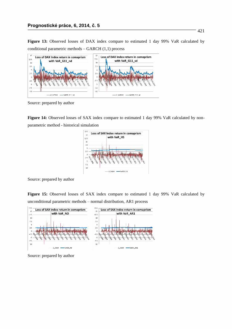
Results of estimation VaR of SAX returns are shown by figure 14, figure 15 and figure 16 and

conclusion from previos paragrph are almost applicable as well. Only all methods of calcualtion are

less effective and resualts are more biased due the fact that all assumptions were not met. Table 4

describes whole picture that Historical simulations is the nearest to theretical expected value of the

brideges however path of estimated loss is far from realized losses on the other hand GARCH model

with Students improvement has still accteble results and realized and estimated loss are the closest.

Figure 11: Observed losses of DAX index compare to estimated 1 day 99% VaR calculated by non-

parametric method - historical simulation


Figure 12: Observed losses of DAX index compare to estimated 1 day 99% VaR calculated by

unconditional parametric methods – normal distribution, AR1 process



Figure 13: Observed losses of DAX index compare to estimated 1 day 99% VaR calculated by

conditional parametric methods – GARCH (1,1) process


Figure 14: Observed losses of SAX index compare to estimated 1 day 99% VaR calculated by non-

parametric method - historical simulation


Figure 15: Observed losses of SAX index compare to estimated 1 day 99% VaR calculated by

unconditional parametric methods – normal distribution, AR1 process



Figure 16: Observed losses of SAX index compare to estimated 1 day 99% VaR calculated by

conditional parametric methods – GARCH (1,1) process


Table 4: Count of situations when realized loss was above estimated VaR


Conclusion

The subject of the article is to analyse the necessity of adopting conditional volatility model for returns

as shows Figure 1. Paper provided the basic demonstrations of theoretical result and illustrated the

main techniques with numerical examples. Figure 7 and 9 proof that GARCH(1,1) is robust enough to

model conditional volatility of DAX revenues despite the fact that ressidual does not follow Gaussian

distribution. Student’s t distribution of innovation improves model sligtly. GARCH (1,1) is easy to

calculate using Matlab, correct volatility on average, exaggerates volatility-of-volatility. Example of

VaR calculating by using GARCH(1,1) shows a substantial gain in accuracy. VaR by GARCH(1,1)

estimeted number of situation when observed loss is higher than estimated VaR worse than historical

simulation however path of this estimation is much closer to real observations.

Conclusion of modeling volatility of capital market is more useful for German economy according

existing and pretty dynamic capital market and model of volatility offered path of instability for whole

DAX SAX

# of observation 1 631 1497

1% of observation 16.3 15.0

VaR99_HS 18 18

VaR99_ND 38 29

VaR99_AR1 38 30

VaR99_G11_nd 33 27

VaR99_G11_sd 26 22

VaR MethodNo of bridge


economy especially in times of global shocks as internet bubble, failure of Lehman Brothers and

sovereign debt crises. Volatility of growth in Slovak economy might be still represented by SAX index

but results are not sufficient supported by significance of estimated parameters. This paper does not

research whether capital market in Slovakia is sufficient or not however general opinion it is not. So to

understand behavior of Slovak economy from perspective of entrepreneur might be worth to dive

deeper to raw data from microeconomics perspective (number of failures or bankrupts of companies)

and consider relations between German DAX due better indication of global crisis. Slovak data seems

to be lagged which indicates that Slovak policy might have applicable alert how the market react to

global crises but without opportunity to change the destiny.

Acknowledgement

This contribution is the result of the project VEGA (2/0160/13) Financial stability and sustainable

economic growth of Slovakia in global economy (Finančná stabilita a udržateľnosť hospodárskeho

rastu Slovenska v podmienkach globálnej ekonomiky)


REFERENCES

[1] Bloomberg. (2014). Deutsche Boerse AG German Stock Index

DAXhttp://www.bloomberg.com/quote/DAX:IND [accessed 1.5.2014]

[2] Burza cenných papierov v Bratislave: Slovenský akciový index SAX

http://www.bsse.sk/Obchodovanie/Indexy/IndexSAX.aspx [accessed 5.11.2014

[3] Bollerslev T. (2011). ARCH and GARCH models

http://public.econ.duke.edu/~boller/Econ.350/talk_garch_11.pdf [accessed 1.5.2014]

[4] Francq, Ch; Zakoian J. M. (2010). GARCH Models Structure, Statistical Inference and Financial

Applications. Lille: John Wiley & Sons Ltd, 2010.

[5] Holton A. (2003). Value-at-risk: Theory and Practice. New York: Academic Press, 2003.

[6] Jorion. P. (2006). Value at Risk, 3rd Ed.: The New Benchmark for Managing Financial Risk. New

York: McGraw Hill Professional, 2006.

[7] Kevin D. (2007). Measuring Market Risk. West Sussex: Wiley & Sons, 2007.

[8] MathWorks (2014). Specify Conditional Mean and Variance

Modelshttp://www.mathworks.com/help/econ/conditional-mean-and-variance-model-for-nasdaq-

returns.html [accessed 15.4.2014]

[9] Yahoo Finance (2014). DAX (^GDAXI) – XETRA

http://finance.yahoo.com/q/hp?s=^GDAXI+Historical+Prices [accessed 15.4.2014]

Kontakt

Ing. Mgr. Matej Štalmach

University of Economics in Bratislava

Faculty of Economic Informatics

Dolnozemská cesta 1/b

852 35 Bratislava 5

Slovakia

e-mail: [email protected]

mobile: 0914373708

http://www.bloomberg.com/quote/DAX:IND


http://public.econ.duke.edu/~boller/Econ.350/talk_garch_11.pdf

http://www.mathworks.com/help/econ/conditional-mean-and-variance-model-for-nasdaq-returns.html

http://www.mathworks.com/help/econ/conditional-mean-and-variance-model-for-nasdaq-returns.html


mailto:[email protected]

Documents

Modeling VaR OF DAX INDEX USING GARCH MODEL · composite conditional mean and variance model using GARCH(1,1) model. We finally apply GARCH methodology to estimate VaR and compare