A comparison of GARCH models for VaR estimation in …630568/FULLTEXT01.pdf · Abstract In this paper the value at risk (VaR) forecasts are compared using three different GARCH models;

2013-06-07

Uppsala University

Department of Statistics

Andreas Johansson, Victor Sowa

Supervisor: Lars Forsberg

A comparison of GARCH models for VaR

estimation in three different markets.

.

Abstract

In this paper the value at risk (VaR) forecasts are compared using three different

GARCH models; ARCH(1), GARCH(1,1) and EGARCH(1,1). The implemented method is a

one-day ahead out of sample forecast of the VaR. The forecasts are evaluated using the

Kupiec test with a five percent significance level. The focus is on three different markets;

commodities, equities and exchange rates.

The goal of this thesis is to answer which of the models; ARCH(1), GARCH(1,1) and

EGARCH(1,1) is best at forecasting the VaR for commodities, equities and exchange rates.

Which assumed distribution for the conditional variance performs the best? Is the normal

distribution or the Student-t a better option when forecasting VaR?

The results shows that the ARCH(1) and EGARCH(1,1) model specifications are good

options for forecasting the VaR for the chosen securities. These models give rise to a

statistical significant forecast for the VaR with only one exception, the exchange rate between

the SEK and USD. The worst performing model is the GARCH(1,1), which showed no

significant results for any security.

The normal distribution is the preferred conditional distribution assumption. In some

securities the Student-t distribution shows a marginally better result, but the normal

distribution is also a valid option in those cases.

Keywords: ARCH, GARCH, EGARCH, Value at Risk, Volatility and Forecasting.

Contents 1. Theory ........................................................................................................................... 1

1.1 Introduction ............................................................................................................. 1

1.2 Value at Risk (VaR) ................................................................................................ 2

1.3 ARCH/GARCH models .......................................................................................... 5

1.4 Earlier Results ......................................................................................................... 8

2. Data/Method ................................................................................................................. 9

2.1 Data ......................................................................................................................... 9

2.2 Descriptive statistics .............................................................................................. 10

2.3 Test of the data ...................................................................................................... 11

2.4 Moving out of sample Forecast ............................................................................. 12

3. Results/Discussion ...................................................................................................... 13

3.1 ARCH(1) results .................................................................................................... 13

3.2 GARCH(1,1) results .............................................................................................. 15

3.3 EGARCH(1,1) results ........................................................................................... 16

4. Conclusion .................................................................................................................. 18

4.1 Summary ............................................................................................................... 18

4.2 Recommendations for investors ............................................................................ 19

5. Acknowledgments ...................................................................................................... 19

6. References ................................................................................................................... 20

7. Appendix ..................................................................................................................... 22

7.1 Return series .......................................................................................................... 22

7.2 Parameter Estimation ............................................................................................ 23

7.3 Comparison of ARCH(1) forecasts vs. the unconditional variance ...................... 27

1

1. Theory

1.1 Introduction

All investors try to maximize their returns on investments while minimizing risks;

therefore the perceived risk is a key ingredient in all investment decisions. The investor will

require a risk premium to invest in risky assets; hence the required returns are higher the more

risk a specific investment contains1. Each investor must choose his or her portfolio carefully

since a large investment in a negatively returning security will generate a large loss and a too

small investment in a good security will generate an opportunity cost. To manage risk is

therefore crucial for maximizing the portfolios return while minimizing losses.

A frequently used risk measure is the value at risk (VaR), which measures the

likelihood that a portfolio will face its worst case outcome over a predetermined time period

and at a predefined confidence level (Angelidis et al., 2004).

One of the reasons why the VaR is such a prevalent method to estimate risk is due to the

regulatory framework created by the Basel committee on Banking Supervision during the

nineties. This regulatory framework forces the banks to calculate VaR for their portfolios,

preventing them from taking on too much financial risk (Basel III, 2010). VaR is a relative

simple concept, which is easy to implement and use for everyday investors.

For the calculation of VaR an investor needs to estimate the securities volatility, i.e.

risk. Empirical studies have concluded that financial instruments have heteroscedasticity in

the variance. To address this observation the autoregressive conditional heteroscedasticity

model (ARCH) and the general autoregressive conditional heteroscedasticity model

(GARCH) were introduced by Engle (1982) and Bollerslev (1986). The family of GARCH

models captures the changing volatility over time, since they are conditional upon

heteroscedasticity (Orhan and Köksal, 2011).

Since the initial introduction of the ARCH and GARCH over 100 new varieties of these

have emerged (Bollerslev, 2010). However there is no definite answer to which of the models

from the GARCH family that is the best at forecasting the volatility for all types of financial

data. Due to the plethora of different GARCH models available the models that have been

examined need to be restricted. This thesis will focus on three of the most commonly used,

1 True if investors are assumed to be rational and risk averse.

2

which are; the ARCH(1), GARCH(1,1) and the EGARCH(1,1) (Bollerslev et al., 2010). The

three models will be used to estimate the VaR with a one-day ahead forecast horizon. Nine

different securities representing three different markets (commodities, equities and currencies)

in the time period June 2009 - April 2013 are used to evaluate the VaR for the different

models.

The goal of this thesis is to answer:

Which of the models; ARCH(1), GARCH(1,1) and EGARCH(1,1) is best at

forecasting the VaR for commodities, equities and exchange rates?

Which assumed distribution for the conditional variance performs the best? Is the

normal distribution or the Student-t a better option when forecasting VaR?

The outline of this paper is as follows. In Section 1 the theoretical framework is

presented along with some earlier results. In Section 2 we describe the data and method that is

used. In Section 3 the main results is discussed and Section 4 contains the concluding

remarks.

1.2 Value at Risk (VaR)

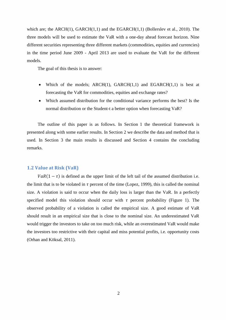
( ) is defined as the upper limit of the left tail of the assumed distribution i.e.

the limit that is to be violated in percent of the time (Lopez, 1999), this is called the nominal

size. A violation is said to occur when the daily loss is larger than the VaR. In a perfectly

specified model this violation should occur with percent probability (Figure 1). The

observed probability of a violation is called the empirical size. A good estimate of VaR

should result in an empirical size that is close to the nominal size. An underestimated VaR

would trigger the investors to take on too much risk, while an overestimated VaR would make

the investors too restrictive with their capital and miss potential profits, i.e. opportunity costs

(Orhan and Köksal, 2011).

3

Figure 1 – VaR for a security. VaR is the minimum amount that will be lost with a probability of τ. (τ = 0.05 in the

figure).

The probability function for VaR can be written as

( ( )) (1)

where is the daily return. ( ) is defined as

( ) (2)

where is the mean of the returns, is the assumed distributions critical value2 with area

and is the volatility obtained from the model estimate (Orhan and Köksal, 2011). The

( ) is the minimum that will be lost with the frequency of . For example, if

$100.000 is invested in a security with a VaR of 4 percent and a of 5 percent. Then the

security would lose a minimum of $4000 five percent of the time.

2 For a normal distribution this would correspond to 1.65 for .

4

In this thesis VaR is evaluated using a likelihood ratio test developed by Kupiec (1995).

This test allows the empirical size to be tested against the nominal size. The test statistic for

this test is the likelihood ratio

((

) (

) (( ) ( ) (3)

where V is the total number of violations in the time period and hence

is the empirical

size. This can be found using the indicator function

{ ( ) ( )

(4)

where receives a value of one if the daily loss is more than the VaR. The total number

of violations are . In a perfectly specified model the probability for a violation is ,

creating the null hypothesis that

, i.e. the empirical size is equal to the nominal size.

The more

deviates from the larger the Kupiec score (K) will become. K is known to

belong to a chi-square distribution with 1 degree of freedom (Orhan and Köksal, 2011). The

commonly used 5 percent significance level is used in this thesis, i.e. if the K value is larger

than 3.84 the null hypothesis will be rejected. If the null hypothesis is rejected, the specific

model is not a suitable specification to estimate the VaR for that security.

There are some flaws in the Kupiec test. Firstly, the test does not take the sequence of

violations into account. If the violations are not independent it may cause a researcher to

underestimate the risk in times of economic uncertainty (Orhan and Köksal, 2011). Secondly,

the Kupiec score is not affected by how large the violation is. This means that a 1 percent

violation or a 4 percent violation will have the same weight (Lehar et al., 2002).

In this thesis the volatility is estimated by using three different types of

ARCH/GARCH models.

5

1.3 ARCH/GARCH models

Different types of autoregressive conditional heteroscedasticity models (ARCH), first

introduced by Engle (1982), are commonly used to estimate risk. The ARCH model expanded

into the generalized autoregressive conditional heteroscedasticity (GARCH) model by

Bollerslev (1986). These models capture the fluctuations in variance over time, which are

present in most financial instruments. Another empirical observation is that the variance is

usually higher during times of turmoil. Nelson (1991) created the exponential GARCH

(EGARCH) model to capture this tendency. An EGARCH model allows positive and negative

shocks3 to have different effects on the estimated variance. The three different model

specifications are presented below.

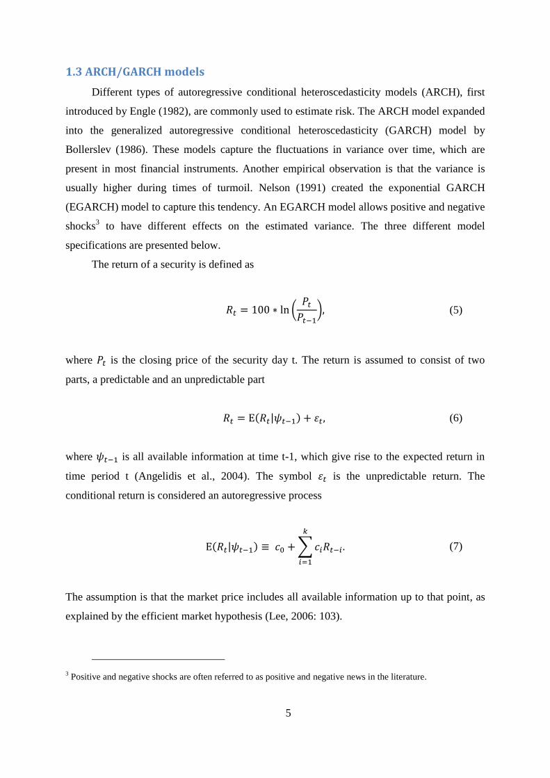
The return of a security is defined as

(

) (5)

where is the closing price of the security day t. The return is assumed to consist of two

parts, a predictable and an unpredictable part

( | ) (6)

where is all available information at time t-1, which give rise to the expected return in

time period t (Angelidis et al., 2004). The symbol is the unpredictable return. The

conditional return is considered an autoregressive process

( | ) ∑

(7)

The assumption is that the market price includes all available information up to that point, as

explained by the efficient market hypothesis (Lee, 2006: 103).

3 Positive and negative shocks are often referred to as positive and negative news in the literature.

6

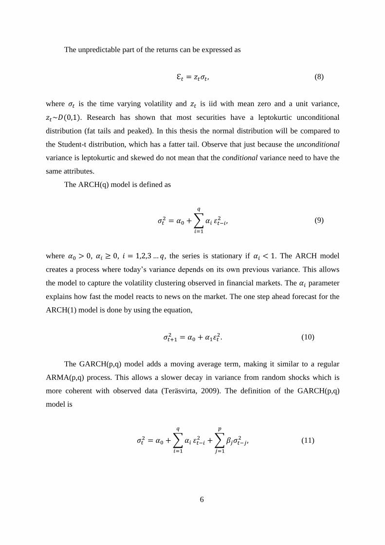
The unpredictable part of the returns can be expressed as

(8)

where is the time varying volatility and is iid with mean zero and a unit variance,

( ). Research has shown that most securities have a leptokurtic unconditional

distribution (fat tails and peaked). In this thesis the normal distribution will be compared to

the Student-t distribution, which has a fatter tail. Observe that just because the unconditional

variance is leptokurtic and skewed do not mean that the conditional variance need to have the

same attributes.

The ARCH(q) model is defined as

∑

(9)

where , , , the series is stationary if . The ARCH model

creates a process where today’s variance depends on its own previous variance. This allows

the model to capture the volatility clustering observed in financial markets. The parameter

explains how fast the model reacts to news on the market. The one step ahead forecast for the

ARCH(1) model is done by using the equation,

(10)

The GARCH(p,q) model adds a moving average term, making it similar to a regular

ARMA(p,q) process. This allows a slower decay in variance from random shocks which is

more coherent with observed data (Teräsvirta, 2009). The definition of the GARCH(p,q)

model is

∑

∑

(11)

7

where , , , , . The process will be stationary

if . If the stationarity condition is fulfilled the conditional variance will converge

towards the unconditional variance

( ). The parameter again explains how fast the

model reacts to news on the market while states how persistent the conditional

heteroscedasticity is over time. If the parameter is large, effects from economic news in the

market will have a tendency to linger. The GARCH(1,1) is the most used model specification,

often used as a benchmark model within this area. The one step ahead forecast for the

GARCH(1,1) model is done by using the equation,

(12)

The EGARCH(p,q) model captures the asymmetric effect on variance from positive and

negative news (Nelson, 1991). From empirical data the market volatility seem to react

differently depending on the sign of the shocks, negative shocks usually results in periods of

higher volatility compared to positive news (Nelson, 1991). By including a third parameter

the EGARCH allows the model to react differently depending on the different type of news.

The EGARCH model is defined as

( ) ∑

(| | (| |)) ∑ ( )

∑

(13)

where

and (| |) will depend on the assumed distribution, for a normal

distribution (| |) √

. If (| | (| |)) the market is returning less than expected,

clearly a negative shock. If the estimation shows that it implies that the model is

symmetric. However, if the estimation shows that it will imply that negative news

cause a higher future volatility than a positive, hence the model is asymmetric. The EGARCH

model differs from the ARCH and GARCH models because the logarithm of the variance is

what is being estimated. By taking the logarithm of the conditional variance it ensures a

positive value. The logarithm also relaxes the parameters constraint; they no longer need to be

positive. and are still expected to have positive values. It is troublesome for inference

and forecasting if they are negative. The however is expected to have a negative value,

8

which means that a negative shock in the market will increase the future volatility

(“MathWorks,” 2013). The EGARCH model is stationary if The one step ahead

forecast for the EGARCH(1,1) model is done by using the equation,

( ) (| | (| |)) (

) . (14)

1.4 Earlier Results

Research in this area has been extensive. There is no definitive conclusion on which

model in the GARCH family that is best suited to forecast the volatility for specific types of

securities. Most research has shown that a leptokurtic conditional distribution is better at

describing the VaR (Angelidis et al., 2004; Orhan and Köksal, 2011; Köksal, 2009; Aloui and

Mabrouk, 2010). Usually the normal distribution is compared against Student-t or the

generalized error distribution (GED).

There is a big difference in which specific GARCH model that performs the best. Orhan

& Köksal (2011) showed that the ARCH(1) model was the best one for estimating risk for

currencies compared to 15 other GARCH models. Köksal (2009) and Hansen & Lunde (2005)

showed that more sophisticated models outperformed the GARCH(1,1) model when

forecasting the ISE-100 index and the DM-$ exchange. A majority of research have

concluded that models, which take information asymmetry into consideration, outperform

symmetric models (Hansen and Lunde, 2005; Aloui and Mabrouk, 2010).

When compared to other families of volatility models the GARCH models outperforms

others such as Black and Scholes models, stochastic volatility models, regime switching

models and grey theorem (Lehar et al., 2002; Kung and Yu, 2008; Luo et al., 2010; Pederzoli,

2006). Ultimately, the GARCH models are still the preferred choice when forecasting VaR.

More recent research has shown that a better estimate of the variance is to use the

realized variance instead of the squared returns (Andersen and Bollerslev, 1998; Hansen et al.,

2012). This is however outside the scope of this paper and we will use the squared returns as

an estimate for the daily variance.

9

2. Data/Method

All calculations are done in Matlab R2012b Simulink version and the MFE toolbox

(“MFE Toolbox,” n.d.).

2.1 Data

The data that have been used were downloaded from Thomson Reuters Datastream

(“Datastream,” n.d.). Financial instruments are chosen to cover different parts of the market

(Table 1). The datasets are divided into three groups; commodities, equities and currencies.

Equities have been selected to represent some of Sweden’s largest companies.

Security Description

CO

MM

OD

ITIE

S

Corn No2 Yellow Corn future

Crude Oil-WTI Is a grade of crude oil used as a benchmark in oil pricing.

Gold Bullion Exchange traded commodity backed by physical gold (USD)

EQU

ITIE

S

Hennes & Mauritz Is a multinational retail-clothing company.

VOLVO Manufacturer of cars, trucks, buses and construction equipment.

Ericsson Company that provides telecommunication equipment.

CU

RR

ENC

IES SEK to EUR Exchange rate between SEK and EUR

SEK to GBP Exchange rate between SEK and GBP

SEK to USD Exchange rate between SEK and USD

Table 1 - The datasets used in this paper to compare the different conditional volatility models. The data is from the

start of June 2009 until the start of April 2013. Only trading days are included in the samples.

Each model is estimated using the adjusted closing price for the last 1000 trading days

for each security4. The data used in the estimates are from the start of June 2009 up to the start

of April 2013 for each dataset.

4 First 500 observations used for the starting estimate, followed by the 500 one-step-ahead forecasts.

10

2.2 Descriptive statistics

n Mean std Min Max Kurtosis Skewness

Corn No2 Yellow 1000 0.04 2.11 -9.32 10.89 5.71 0.06

Crude Oil-WTI 1000 0.03 1.85 -9.04 8.95 4.94 -0.15

Gold Bullion 1000 0.05 1.07 -5.87 3.79 5.83 -0.65

Hennes & Mauritz 1000 0.03 1.49 -7.58 8.04 6.64 -0.17

VOLVO 1000 0.06 2.18 -9.92 9.61 4.42 0.02

Ericsson 1000 0.01 1.87 -15.18 10.21 10.42 -0.56

SEK to EUR 1000 -0.03 0.47 -2.01 1.99 4.10 -0.01

SEK to GBP 1000 -0.02 0.67 -2.27 2.84 3.76 0.11

SEK to USD 1000 -0.02 0.85 -3.19 3.25 3.64 0.06 Table 2 - Descriptive statistics. All calculations are done for the last 1000 observations for each dataset, capturing the

first 500 observations used for the first model estimation plus the 500 rolling forecasts. (Everything is calculated using

percentage points 1 = 1%).

Figure 2 – Two examples of the returns. Each plot uses the last 1000 observations for each dataset, capturing the first

500 observations used for the first model estimation plus the 500 rolling forecasts. The graph for each security is

available in Appendix 8.1.

Each dataset has a mean return very close to zero and all the time series shows signs of

heteroscedasticity, as expected (Figure 2). Among the commodities and equities there are

large differences between the minimum and maximum values. This is in contrast with the

relative small maximum and minimum values in the exchange rates (Table 2). The standard

deviations are similar between the different securities though, which suggest that extreme

values are more common among commodity and equity prices than exchange rates. All

securities have a positive excess kurtosis suggesting that they have leptokurtic distributions.

Most of the securities also have skewed distributions, some are positive and some are

negative. This is a bit surprising when earlier work has shown that securities have a negative

skewness in returns (Orhan and Köksal, 2011).

11

2.3 Test of the data

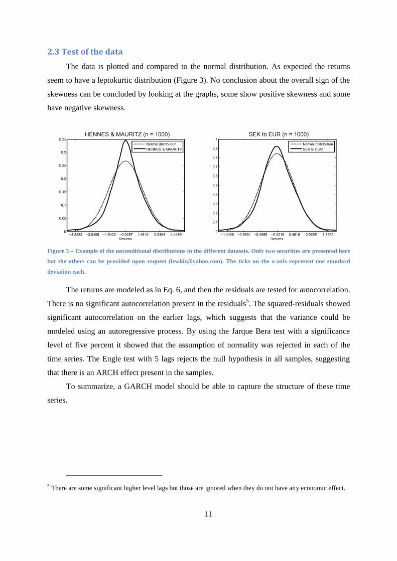
The data is plotted and compared to the normal distribution. As expected the returns

seem to have a leptokurtic distribution (Figure 3). No conclusion about the overall sign of the

skewness can be concluded by looking at the graphs, some show positive skewness and some

have negative skewness.

Figure 3 – Example of the unconditional distributions in the different datasets. Only two securities are presented here

but the others can be provided upon request ([email protected]). The ticks on the x-axis represent one standard

deviation each.

The returns are modeled as in Eq. 6, and then the residuals are tested for autocorrelation.

There is no significant autocorrelation present in the residuals5. The squared-residuals showed

significant autocorrelation on the earlier lags, which suggests that the variance could be

modeled using an autoregressive process. By using the Jarque Bera test with a significance

level of five percent it showed that the assumption of normality was rejected in each of the

time series. The Engle test with 5 lags rejects the null hypothesis in all samples, suggesting

that there is an ARCH effect present in the samples.

To summarize, a GARCH model should be able to capture the structure of these time

series.

5 There are some significant higher level lags but those are ignored when they do not have any economic effect.

12

2.4 Moving out of sample Forecast

Figure 4 – Flowchart of the method used to compare the VaR between the models. Each model, with the two different conditional distribution assumptions is estimated using a sample

size of 500 observations, the estimation window. Each model is estimated 500 times each, moving the estimation window one step forward each time. Each model estimate is used to do

a one-step-ahead forecast of the VaR. The forecasted VaR is then compared to the actual observed value in the next time period. The violations, larger losses than the predicted VaR,

are summarized and the Kupiec score is calculated to compare the different models.

13

A common way to test the predictive power of a model is to do a sequence of out of

sample forecasts (Figure 5). The estimation window, in the initial stage, consists of the first

500 days of our sample. With those 500 days the 501st day’s variance is forecasted and

compared to the observed variance for that day. The observed value for the 501st observation

is then included while the first observation in the initial estimation window is dropped,

making the estimation window again consist of 500 observations but now from the second to

the 501st day and the 502nd is forecasted. This is done until the entire forecast window of 500

observations has been forecasted (Figure 4).

Figure 5 – A rolling forecast is estimated for each dataset. 500 observations are used for the model estimate, which is

then used to predict the next day’s variance. Estimated VaR is then compared with the actual observed returns for the

next period. Then the rolling forecast is moved one step forward and the procedure is repeated. A total of 500

predictions are calculated for each model and the number of violations, Rt+1 < VaR, is summarized.

Each model is estimated using the three different GARCH models. The estimated model

is then used to make an out of sample prediction, which is compared to the observed value

(Hansen and Lunde, 2005).

3. Results/Discussion

3.1 ARCH(1) results

Each distribution is calculated by using a one-step-ahead out of sample forecast that is

compared to the observed value. The expected VaR for next time period can then be evaluated

by comparing the nominal size against the empirical size.

The Kupiec test shows that the null hypothesis,

, cannot be rejected with a 5

percent significance for the ARCH(1) models with one exception, the exchange rate between

14

SEK and USD (Table 3). Comparing this with the Student-t distribution where the null

hypothesis is rejected in all except three securities. This implies that the normal distribution is

a more accurate conditional distribution assumption than the Student-t when predicting VaR

for these securities. This is inconsistent with earlier results that have shown that the Student-t

is overall better at forecasting VaR, since it captures the leptokurtic distribution in returns6.

CO

MM

OD

ITIE

S

Corn No2 Yellow Crude Oil-WTI Gold Bullion

NORMAL STUDENTS NORMAL STUDENTS NORMAL STUDENTS

V/N 3.8% 2.4% 4.6% 3.0% 6.2% 3.2%

Kupiec 1.6 8.7 0.2 4.9 1.4 3.9

EQU

ITIE

S

Hennes & Mauritz VOLVO Ericsson


V/N 4.8% 2.6% 6.2% 4.6% 5.0% 2.4%

Kupiec 0.04 7.3 1.4 0.2 0.0 8.7

CU

RR

ENC

IES

SEK to EUR SEK to GBP SEK to USD


V/N 5.2% 4.0% 3.4% 3.2% 2.6% 2.6%

Kupiec 0.04 1.1 3.0 3.9 7.3 7.3

Table 3 - ARCH(1) out of sample forecast results. The VaR is estimated using a nominal size of five percent, τ = 0.05.

This means that the null hypothesis, H0: V/N = τ, is rejected at a five percent significance level if the Kupiec score is

larger than 3.8 (Acceptance of the null hypothesis is green and rejection is red).

The ARCH(1) model seem to result in a rigid one step ahead forecast, it only seem to

react during periods of large changes in variance (Figure 6). All the ARCH(1) models have a

relative small α1 parameter value, so only large shocks will have an effect on the forecast

(Appendix 8.2). It results in a forecast very close to the unconditional variance (Appendix

8.3).

6 Just because the unconditional distribution shows a leptokurtic distribution does not mean that the conditional

distribution need to have the same distribution though.

15

Figure 6 – Two examples of the ARCH(1) out of sample forecast with the normal distribution assumption. The red

dots represent the forecasted values and the blue line is the observed variance7. Note that the last 500 observations are

used for the one-step-ahead forecast for each dataset.

3.2 GARCH(1,1) results

In comparison with the ARCH(1) model the GARCH(1,1) seems to be a worse option

when forecasting VaR. The null hypothesis is rejected in all Kupiec tests. This implies that the

GARCH(1,1) is bad at forecasting the VaR for the selected securities (Table 4).

CO

MM

OD

ITIE

S



V/N 12.4% 13.2% 8.8% 9.0% 16.2% 13.6%

Kupiec 41.6 49.8 12.5 13.75 85.3 54.1

EQU

ITIE

S

HENNES & MAURITZ VOLVO ERICSSON


V/N 11.4% 8.4% 16.4% 15.6% 11.6% 13.6%

Kupiec 32.2 10.2 87.9 77.6 34.0 54.1

CU

RR

ENC

IES



V/N 12.0% 11.2% 14% 13.0% 16.4% 16.0%

Kupiec 37.7 30.4 58.6 47.7 87.9 82.7

Table 4 - GARCH(1,1) out of sample forecast results. The VaR is estimated using a nominal size of five percent, τ =

0.05. This means that the null hypothesis, H0: V/N = τ, is rejected at a five percent significance level if the Kupiec

score is larger than 3.8 (Acceptance of the null hypothesis is green and rejection is red).

7 The other print outs are available upon request ([email protected]).

16

Looking closer at the empirical size,

, the GARCH(1,1) model underestimates the

potential variance in the next period (Table 4). The graph of the predicted values show that

the forecasted variance is very close to today’s value, meaning that whenever the variance

deviates from today’s variance the forecast fails (Figure 7).

Figure 7 - Two examples of the GARCH(1,1) out of sample forecast with the normal distribution assumption. The red

dots represent the forecasted values and the blue line is the observed variance8. Notice that all the predicted values are

shifted one step to the right of the observed variance.

In contrast to the ARCH(1) model there is no clear conclusion on which distribution is

the best in forecasting the VaR in a GARCH(1,1) model.

3.3 EGARCH(1,1) results

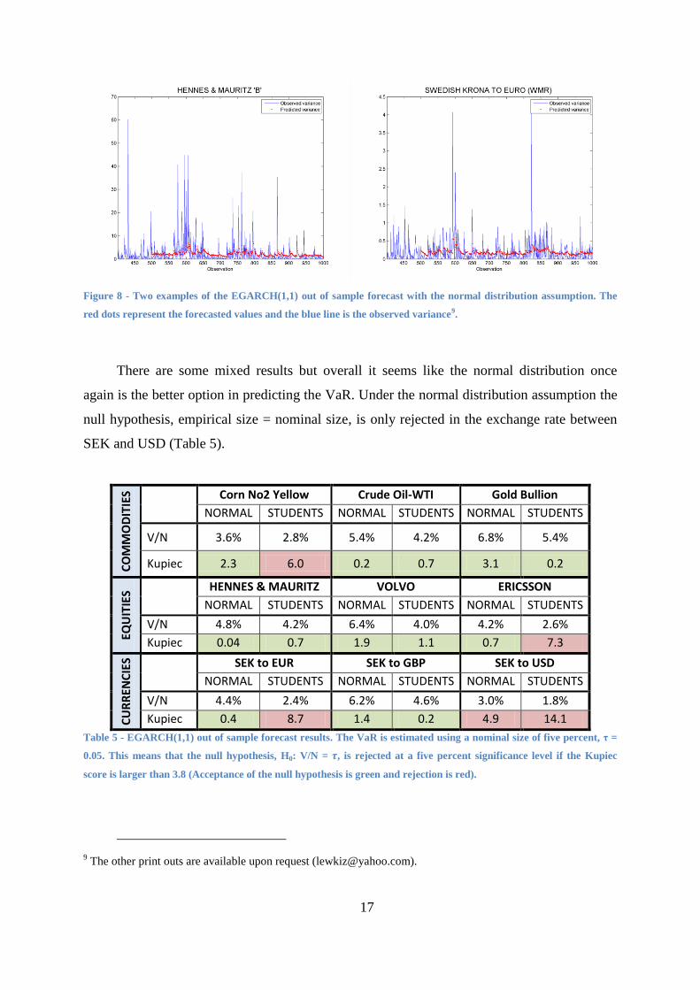
The graphed forecasts indicates that the EGARCH(1,1) is very good at predicting the

next periods variance (Figure 8). This is confirmed by the Kupiec test where the null

hypothesis is only rejected in 5 out of 18 models (Table 5).


17

Figure 8 - Two examples of the EGARCH(1,1) out of sample forecast with the normal distribution assumption. The

red dots represent the forecasted values and the blue line is the observed variance9.

There are some mixed results but overall it seems like the normal distribution once

again is the better option in predicting the VaR. Under the normal distribution assumption the

null hypothesis, empirical size = nominal size, is only rejected in the exchange rate between

SEK and USD (Table 5).

CO

MM

OD

ITIE

S Corn No2 Yellow Crude Oil-WTI Gold Bullion


V/N 3.6% 2.8% 5.4% 4.2% 6.8% 5.4%

Kupiec 2.3 6.0 0.2 0.7 3.1 0.2

EQU

ITIE

S HENNES & MAURITZ VOLVO ERICSSON


V/N 4.8% 4.2% 6.4% 4.0% 4.2% 2.6%

Kupiec 0.04 0.7 1.9 1.1 0.7 7.3

CU

RR

ENC

IES SEK to EUR SEK to GBP SEK to USD


V/N 4.4% 2.4% 6.2% 4.6% 3.0% 1.8%

Kupiec 0.4 8.7 1.4 0.2 4.9 14.1

Table 5 - EGARCH(1,1) out of sample forecast results. The VaR is estimated using a nominal size of five percent, τ =

0.05. This means that the null hypothesis, H0: V/N = , is rejected at a five percent significance level if the Kupiec

score is larger than 3.8 (Acceptance of the null hypothesis is green and rejection is red).


18

The parameter estimates are unstable for some of the EGARCH(1,1) models (Appendix

8.2). It is probably due to the logarithmic transformation and the problems that arise when

there are periods with zero returns. Sometimes the estimation procedure hit the parameter

restrictions, which also contributes to the unstable parameter estimations.

4. Conclusion

4.1 Summary

The results shows that the best models to forecast the VaR for these securities are the

ARCH(1) and the EGARCH(1,1) model. These models are good options for each security

with one exception, the exchange rate SEK to USD. The good results of the EGARCH model

confirms earlier results, models that take asymmetry into consideration outperforms

symmetric models. Even if the empirical size is very similar to the ARCH(1) model, the

EGARCH(1,1) seem to be better at following the currently present variance (Figure 8). This

suggest that the EGARCH(1,1) is better at adjusting for the heteroscedasticity in variance in

comparison to the ARCH(1) model.

The worst performing model is the GARCH(1,1), which showed poor results for all

securities. This is a bit surprising when the GARCH(1,1) model is often used as a benchmark

in this area of research. Orhan & Köksal (2011) showed that the ARCH(1) model

outperformed other GARCH models when looking at exchange rates, so even if it is

uncommon that the ARCH(1) outperforms the GARCH(1,1) model it is still plausible.

The conditional normal distribution shows better results than the Student-t assumption

with few exceptions. This is in contrast with earlier results that mostly have shown that the

Student-t is a better option.

19

4.2 Recommendations for investors

The best performing model for each security is summarized in Table 6. Overall the

ARCH(1) and EGARCH(1,1) models are very close in their empirical size. The ARCH(1)

model is easier to estimate than the EGARCH(1,1), so for a quick estimate the ARCH(1)

model with conditional normal distribution is a good choice10

.

The EGARCH(1,1) seem to be better at adjusting for current volatility in comparison to

the ARCH(1) model (Figure 8). It means that the EGARCH(1,1) is quicker to adjust when

structural breaks happens. Our final recommendation is therefore to use the EGARCH(1,1)

model with the appropriate distribution assumption.

Model Distribution V/N

Corn No2 Yellow ARCH(1) Normal 3.8%

Crude Oil-WTI ARCH(1)

EGARCH(1,1) Normal Normal

4.6% 5.4%

Gold Bullion EGARCH(1,1) Student-t 5.4%

Hennes & Mauritz

ARCH(1) EGARCH(1,1)

Normal Normal

4.8% 4.8%

VOLVO ARCH(1) Student-t 4.6%

Ericsson ARCH(1) Normal 5.0%

SEK to EUR ARCH(1) Normal 5.2%

SEK to GBP EGARCH(1,1) Student-t 4.6%

SEK to USD EGARCH(1,1) Normal 3.0%* Table 6 – The best performing models for VaR estimation for each security. Note that there are very small differences

between the ARCH(1) and the EGARCH(1,1) empirical size. *) It is significantly different from the nominal size of 5

percent.

5. Acknowledgments

Oscar Andersson, Johan Sowa and Rebecca Tingvall.

10 In these samples the ARCH(1) model makes forecasts very close to the unconditional variance. This suggests

that the average variance for the last trading days should give a good estimate for the next period’s variance

(Appendix 8.3). This implies that an even easier way to forecast the VaR is to use the unconditional variance

instead of the ARCH(1) estimate.

20

6. References

Aloui, C., Mabrouk, S., 2010. Value-at-risk estimations of energy commodities via long-

memory, asymmetry and fat-tailed GARCH models. Energy Policy 38, 2326–2339.

Andersen, T.G., Bollerslev, T., 1998. Answering the skeptics: Yes, standard volatility models

do provide accurate forecasts. International Economic Review 39, 885.

Angelidis, T., Benos, A., Degiannakis, S., 2004. The use of GARCH models in VaR

estimation. STAT METHODOL 1, 105–128.

Badescu, A.M., Kulperger, R.J., 2008. GARCH option pricing: A semiparametric approach.

Insurance Mathematics and Economics 43, 69–84.

Basel III: A global regulatory framework for more resilient banks and banking systems,

2010. . Bank for international settlements, Basel, Switzerland.

Bollerslev, T., 1986. Generalized autoregressive conditional heteroscedasticity. Journal of

econometrics 31, 307–327.

Bollerslev, T., 2010. Glossary to ARCH (GARCH).

Bollerslev, T., Russell, J., Watson, M., 2010. Volatility and Time Series Econometrics.

Oxford University Press.

Datastream [WWW Document], n.d. URL

https://www.thomsonone.com/DirectoryServices/2006-04-

01/Web.Public/Login.aspx?brandname=datastream&version=3.6.6.18338&protocol=0

(accessed 3.27.13).

Engle, R.F., 1982. Autoregressive Conditional Heteroscedasticity with Estimates of the

Variance of United Kingdom Inflation. Econometrica 50, 987–1007.

Hansen, P.R., Huang, Z., Shek, H. howan, 2012. Realized GARCH: a joint model for returns

and realized measures of volatility. Journal of Applied Econometrics 27, 877–906.

Hansen, P.R., Lunde, A., 2005. A forecast comparison of volatility models: does anything

beat a GARCH(1,1)? Journal of Applied Econometrics 20, 873–889.

Kung, L.-M., Yu, S.-W., 2008. Prediction of index futures returns and the analysis of financial

spillovers—A comparison between GARCH and the grey theorem. European Journal

of Operational Research 186, 1184–1200.

Kupiec, P.H., 1995. Techniques for verifying the accuracy of risk measurement models.

Board of Governors of the Federal Reserve System (U.S.), Finance and Economics

Discussion Series: 95-24, 1995.

21

Köksal, B., 2009. A Comparison of Conditional Volatility Estimators for the ISE National

100 Index Returns. Journal of Economic and social research 11, 1.

Lee, C.F., 2006. Encyclopedia of finance. Springer, New York.

Lehar, A., Scheicher, M., Schittenkopf, C., 2002. GARCH vs. stochastic volatility: Option

pricing and risk management. Journal of Banking and Finance 26, 323–345.

Lopez, J.A., 1999. Methods for Evaluating Value-at-Risk Estimates. Economic Review

(03630021) 3.

Luo, C., Seco, L.A., Wang, H., Wu, D.D., 2010. Risk modeling in crude oil market: a

comparison of Markov switching and GARCH models. Kybernetes 39, 750–769.

MathWorks [WWW Document], 2013. . MathWorks. URL

http://www.mathworks.se/help/econ/egarch-model.html (accessed 4.9.13).

MFE Toolbox [WWW Document], n.d. Kevin Sheppard. URL

http://www.kevinsheppard.com/wiki/MFE_Toolbox (accessed 4.8.13).

Nelson, D.B., 1991. Conditional Heteroscedasticity in Asset Returns: A New Approach.

Econometrica 59, 347–370.

Orhan, M., Köksal, B., 2011. A comparison of GARCH models for VaR estimation. eswa

2012, 2582–3592.

Pederzoli, C., 2006. Stochastic volatility and GARCH: a comparison based on UK stock data.

European Journal of Finance 12, 41–59.

Teräsvirta, T., 2009. An Introduction to Univariate GARCH Models, in: Mikosch, T., Kreiß,

J.-P., Davis, R.A., Andersen, T.G. (Eds.), Handbook of Financial Time Series.

Springer Berlin Heidelberg, pp. 17–42.

22

7. Appendix

7.1 Return series

Figure 9 - Time series data of the returns for the first six securities examined in this thesis. Each plot uses the last 1000

observations for each dataset, capturing the first 500 observations used for the first model estimation plus the 500

rolling forecasts.

23

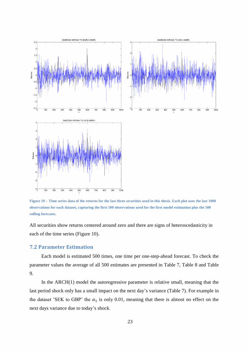
Figure 10 – Time series data of the returns for the last three securities used in this thesis. Each plot uses the last 1000

observations for each dataset, capturing the first 500 observations used for the first model estimation plus the 500

rolling forecasts.

All securities show returns centered around zero and there are signs of heteroscedasticity in

each of the time series (Figure 10).

7.2 Parameter Estimation

Each model is estimated 500 times, one time per one-step-ahead forecast. To check the

parameter values the average of all 500 estimates are presented in Table 7, Table 8 and Table

9.

In the ARCH(1) model the autoregressive parameter is relative small, meaning that the

last period shock only has a small impact on the next day’s variance (Table 7). For example in

the dataset ’SEK to GBP’ the is only 0.01, meaning that there is almost no effect on the

next days variance due to today’s shock.

24

ARCH - 'Normal' ARCH - 'Student-t'

Security α0 α1 Security α0 α1

Corn 4.26

(0.32) 0.05

(0.03) Corn

4.61 (0.28)

0.05 (0.03)

Oil 3.35

(0.27) 0.09

(0.07) Oil

3.42 (0.14)

0.11 (0.05)

Gold 1.22

(0.11) 0.05

(0.02) Gold

1.34 (0.18)

0.08 (0.05)

H&M 1.98

(0.11) 0.26

(0.07) H&M

2.26 (0.25)

0.24 (0.06)

VOLVO 4.53 (0.37)

0.13 (0.04)

VOLVO 4.62

(0.40) 0.13

(0.04)

Ericsson 3.83

(0.60) 0.05

(0.04) Ericsson

3.78 (0.56)

0.11 (0.04)

SEK to EUR 0.16

(0.02) 0.20

(0.03) SEK to EUR

0.16 (0.02)

0.18 (0.03)

SEK to GBP 0.43

(0.05) 0.01

(0.01) SEK to GBP

0.42 (0.05)

0.02 (0.02)

SEK to USD 0.72

(0.05) 0.04

(0.04) SEK to USD

0.72 (0.04)

0.04 (0.04)

Table 7 – Average parameter values for the 500 estimations of the rolling forecast for each ARCH(1) model. Standard

deviation is within parenthesis.

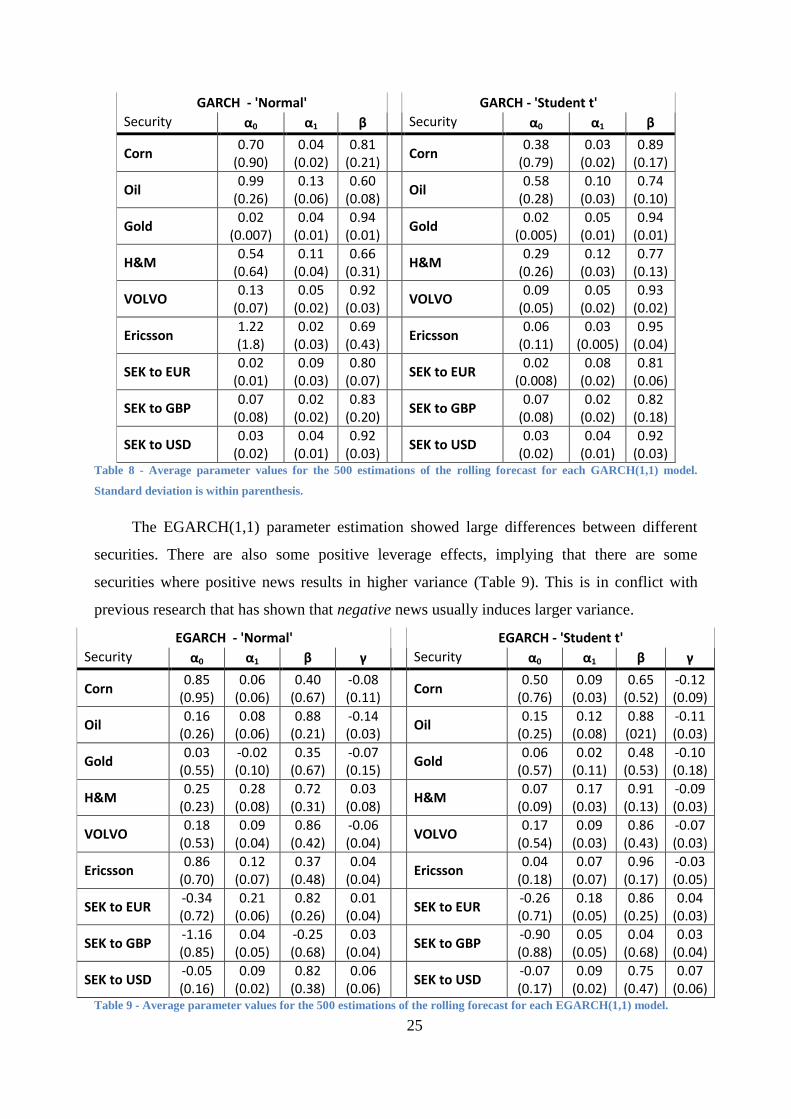
The GARCH(1,1) autoregressive parameter is still very small but the moving average

term is very large (Table 8). The sum of and β decides how fast a shock returns to the long

run variance. This suggests that a shock has a long lasting effect. Also when the β is large, the

last days shock has a very strong influence on the next day’s variance, meaning that the last

shock will have a huge impact on the next day’s variance11

. This is very clear when looking at

the forecast series in the GARCH(1,1) model. The prediction is usually very close to today’s

variance (Figure 7).

11 In the forecast.

25

GARCH - 'Normal'

GARCH - 'Student t'

Security α0 α1 β Security α0 α1 β

Corn 0.70

(0.90) 0.04

(0.02) 0.81

(0.21)

Corn 0.38

(0.79) 0.03

(0.02) 0.89

(0.17)

Oil 0.99

(0.26) 0.13

(0.06) 0.60

(0.08)

Oil 0.58

(0.28) 0.10

(0.03) 0.74

(0.10)

Gold 0.02

(0.007) 0.04

(0.01) 0.94

(0.01)

Gold 0.02

(0.005) 0.05

(0.01) 0.94

(0.01)

H&M 0.54

(0.64) 0.11

(0.04) 0.66

(0.31)

H&M 0.29

(0.26) 0.12

(0.03) 0.77

(0.13)

VOLVO 0.13

(0.07) 0.05

(0.02) 0.92

(0.03)

VOLVO 0.09

(0.05) 0.05

(0.02) 0.93

(0.02)

Ericsson 1.22 (1.8)

0.02 (0.03)

0.69 (0.43)

Ericsson

0.06 (0.11)

0.03 (0.005)

0.95 (0.04)

SEK to EUR 0.02

(0.01) 0.09

(0.03) 0.80

(0.07)

SEK to EUR 0.02

(0.008) 0.08

(0.02) 0.81

(0.06)

SEK to GBP 0.07

(0.08) 0.02

(0.02) 0.83

(0.20)

SEK to GBP 0.07

(0.08) 0.02

(0.02) 0.82

(0.18)

SEK to USD 0.03

(0.02) 0.04

(0.01) 0.92

(0.03)

SEK to USD 0.03

(0.02) 0.04

(0.01) 0.92

(0.03) Table 8 - Average parameter values for the 500 estimations of the rolling forecast for each GARCH(1,1) model.

Standard deviation is within parenthesis.

The EGARCH(1,1) parameter estimation showed large differences between different

securities. There are also some positive leverage effects, implying that there are some

securities where positive news results in higher variance (Table 9). This is in conflict with

previous research that has shown that negative news usually induces larger variance.

EGARCH - 'Normal'

EGARCH - 'Student t'

Security α0 α1 β γ Security α0 α1 β γ

Corn 0.85

(0.95) 0.06

(0.06) 0.40

(0.67) -0.08 (0.11)

Corn

0.50 (0.76)

0.09 (0.03)

0.65 (0.52)

-0.12 (0.09)

Oil 0.16

(0.26) 0.08

(0.06) 0.88

(0.21) -0.14 (0.03)

Oil

0.15 (0.25)

0.12 (0.08)

0.88 (021)

-0.11 (0.03)

Gold 0.03

(0.55) -0.02 (0.10)

0.35 (0.67)

-0.07 (0.15)

Gold

0.06 (0.57)

0.02 (0.11)

0.48 (0.53)

-0.10 (0.18)

H&M 0.25

(0.23) 0.28

(0.08) 0.72

(0.31) 0.03

(0.08)

H&M 0.07

(0.09) 0.17

(0.03) 0.91

(0.13) -0.09 (0.03)

VOLVO 0.18

(0.53) 0.09

(0.04) 0.86

(0.42) -0.06 (0.04)

VOLVO

0.17 (0.54)

0.09 (0.03)

0.86 (0.43)

-0.07 (0.03)

Ericsson 0.86

(0.70) 0.12

(0.07) 0.37

(0.48) 0.04

(0.04)

Ericsson 0.04

(0.18) 0.07

(0.07) 0.96

(0.17) -0.03 (0.05)

SEK to EUR -0.34 (0.72)

0.21 (0.06)

0.82 (0.26)

0.01 (0.04)

SEK to EUR

-0.26 (0.71)

0.18 (0.05)

0.86 (0.25)

0.04 (0.03)

SEK to GBP -1.16 (0.85)

0.04 (0.05)

-0.25 (0.68)

0.03 (0.04)

SEK to GBP

-0.90 (0.88)

0.05 (0.05)

0.04 (0.68)

0.03 (0.04)

SEK to USD -0.05 (0.16)

0.09 (0.02)

0.82 (0.38)

0.06 (0.06)

SEK to USD

-0.07 (0.17)

0.09 (0.02)

0.75 (0.47)

0.07 (0.06)

Table 9 - Average parameter values for the 500 estimations of the rolling forecast for each EGARCH(1,1) model.

26

The average parameter values seem to be very plausible. Problems arise when each

single parameter-estimation is examined. The value of the estimated parameter fluctuates

depending on the exact sample used (Figure 11). This fluctuation in parameter values are

present in most samples but it is clearly the worst in the EGARCH(1,1) models (Table 9).

There are some parameter-value-spikes present in most EGARCH model estimates. This

could be due to a couple of reasons. Firstly, the EGARCH uses a logarithmic transformation,

which means that periods with zero returns results in undefined values. Secondly, the

optimization code hit the hard coded parameter restrictions during some sample estimations,

creating artificial boundaries on the parameter values. Finally, there might be some problems

with the starting values used in the optimization process, resulting in miss defined maximum

likelihood estimates.

All models are approximations of reality. A good model should be stable and give rise

to similar results no matter which sample that is used. These fluctuations suggest that the

EGARCH model might be problematic to use when forecasting the VaR for these securities.

This is outside the scope of this paper but could be interesting to investigate in future

research.

Figure 11 – Example of the two worst performing parameter estimation. Both are EGARCH(1,1) models under

normal conditional distribution assumption (shows similar results with the Student-t). The other EGARCH models

only have a couple of spikes around a baseline. Each line represents the parameter value during each step-ahead

forecast of the model.

27

7.3 Comparison of ARCH(1) forecasts vs. the unconditional variance

The ARCH(1) model makes forecasts very close to the unconditional variance. To test if

this is true; the same estimate for the VaR was done using the unconditional variance as the

forecast of the next period’s variance. As shown by Table 10 the unconditional variance

shows similar results as the ARCH(1) model. This is not a surprise when the alpha values are

very small in the different ARCH(1) models (Appendix 8.2), meaning that the unconditional

variance will have a large impact on the forecasted values.

CO

MM

OD

ITIE

S


ARCH(1) Avg. Var. ARCH(1) Avg. Var. ARCH(1) Avg. Var.

V/N 3.8% 3.6% 4.6% 4.4% 6.2% 6.0%

Kupiec 1.6 2.3 0.2 0.4 1.4 1.0

EQU

ITIE

S

Hennes & Mauritz VOLVO Ericsson


V/N 4.8% 4.6% 6.2% 6.2% 5.0% 5.4%

Kupiec 0.04 0.2 1.4 1.4 0.0 0.2

CU

RR

ENC

IES



V/N 5.2% 4.2% 3.4% 3.4% 2.6% 2.4%

Kupiec 0.04 0.7 3.0 3.0 7.3 8.7

Table 10 – A comparison between the ARCH(1) forecast and the unconditional variance (Average Variance) for the

forecast. Both are using the conditional normal distribution assumption and a moving rolling forecast of 500

observations. Kupiec test with 5% significance level is used to evaluate the VaR with a 5% nominal size. H0: V/N = τ,

green acceptance, red rejection.

Documents

A comparison of GARCH models for VaR estimation in …630568/FULLTEXT01.pdf · Abstract In this paper the value at risk (VaR) forecasts are compared using three different GARCH models;