Testing for Slope Heterogeneity Bias in Panel DataModels∗

Murillo Campello, Antonio F. Galvao, and Ted Juhl

Abstract

Standard econometric methods can overlook individual heterogeneity in empiricalwork, generating inconsistent parameter estimates in panel data models. We proposethe use of methods that allow researchers to easily identify, quantify, and address es-timation issues arising from individual slope heterogeneity. We first characterize thebias in the standard fixed effects estimator when the true econometric model allowsfor heterogeneous slope coefficients. We then introduce a new test to check whetherthe fixed effects estimation is subject to heterogeneity bias. The procedure tests thepopulation moment conditions required for fixed effects to consistently estimate therelevant parameters in the model. We establish the limiting distribution of the test,and show that it is very simple to implement in practice. We also generalize the testto allow for cross-section dependence in the errors and a form of endogeneity. Exam-ining firm investment models to showcase our approach, we show that heterogeneitybias-robust methods identify cash flow as a more important driver of investment thanpreviously reported. Our study demonstrates analytically, via simulations, and empir-ically the importance of carefully accounting for individual specific slope heterogeneityin drawing conclusions about economic behavior.

Key Words: Testing, fixed effects, individual heterogeneity, bias, slope heterogeneity

JEL Classification: C12, C23

∗The authors are grateful to Cecilia Bustamante, Zongwu Cai, George Gao, Erasmo Giambona, HyunseobKim, Oliver Linton, Whitney Newey, Suyong Song, Albert Wang, Zhijie Xiao, and the participants at semi-nars at Chapman University, Claremont McKenna College, University of Iowa, University of Kansas, Univer-sity Wisconsin-Milwaukee, 25th Midwest Econometrics Group, and NY Camp Econometrics VIII for theirconstructive comments and suggestions. Murillo Campello, 369 Sage Hall, Samuel Curtis Johnson GraduateSchool of Management, Cornell University, Ithaca, NY 14853; Tel (607)-255-1282; (campello@cornell.edu).Antonio Galvao, Tippie College of Business, University of Iowa, W284 Pappajohn Business Building, 21 E.Market Street, Iowa City, IA 52242; Tel (319) 335-1810; (antonio-galvao@uiowa.edu). Ted Juhl, Departmentof Economics, University of Kansas, 415 Snow, Lawrence, KS 66045; Tel (785)-864-2849; (juhl@ku.edu).

1 Introduction

With the increasing availability of large, comprehensive databases, researchers seek to iden-

tify and understand richer nuances of microeconomic behavior. Recent computable general

equilibrium models introduce behavioral heterogeneity across firms and agents when gener-

ating distributions of potential outcomes. To the extent that economic decisions are shaped

by these considerations it is natural to consider a methodology that allows for information

about the distribution of model inputs (e.g., input variances and covariances) to be incor-

porated in empirical parameter estimates. This paper shows that estimation methods that

ignore relations between model input distribution and parameters can lead to biased infer-

ences about microeconomic behavior. Understanding and addressing these problems is key

to advancing empiricists’ ability to inform theory development.

Empirical work in economics often relies on methods that assume a large degree of ho-

mogeneity across individuals. One way to account for some degree of heterogeneity in panel

data models is to use the ordinary least squares fixed effects (OLS-FE) estimator. When

estimating individual-fixed effects models, one often imposes concomitant assumptions of

heterogeneous “intercepts” and homogeneous “slope coefficients” across individuals.

This paper characterizes and addresses the issues of estimation and inference of econo-

metric models in the presence of heterogeneity in individual policy responses (“slope co-

efficients”). We contribute to the literature by proposing the use of methods that allow

researchers to easily identify, quantify, and address estimation issues arising from individ-

ual heterogeneity. More generally, our analysis warns researchers about imposing arbitrary

homogeneity restrictions when studying complex economic behavior.

We start by describing two main results. First, we show analytically how the presence

of individual slope heterogeneity may bias the policy estimates obtained under the OLS-FE

framework. Second, we discuss alternative methods that account for slope heterogeneity and

1

produce consistent estimates for the parameters of interest. To do so, we analyze a simple

panel data model from which we recover the parameters of interest for each individual. This

allows us to study individual slope heterogeneity in detail. To summarize the coefficients of

interest, we employ a simple statistic: the mean group (MG) estimator. In its simplest form,

the MG estimator is the average of the response (slope) coefficients of each of the individ-

uals used to fit an empirical model (see Pesaran (2006)). This estimator is in the class of

minimum distance estimators and has several attractive features.1 Our analysis shows that

the MG method has estimation and inference properties that generally dominate those of

the OLS-FE estimator when firms respond differently to innovations to a model driver. At

the same time, we provide researchers with diagnostic tests to determine whether the use of

the OLS-FE approach is warranted in their particular applications.

Importantly, the main contribution of this paper is to develop a new test to identify

whether the presence of slope heterogeneity in the data will cause bias in OLS-FE estimates.

The OLS-FE is asymptotically biased when the heterogeneous coefficients are correlated

with the variance of the regressors. Accordingly, we propose a test for the null hypothesis

that there is no correlation between variances of the data and the heterogeneous parame-

ters. Hence, our procedure tests the population moment conditions required for fixed effects

to consistently estimate the relevant parameters in the model. We describe the associated

test statistic and derive its limiting distribution. This test is particularly useful for applied

researchers in that it follows a standard chi-square distribution, for which critical values are

tabulated and widely available.

We also generalize the test to allow for cross-sectional dependence in the errors and in

the regressors, and also a form of endogeneity. We show that these extensions can be easily

1First, the MG estimator is easy to implement and its computation is no more difficult than that of theOLS-FE. Second, the economic interpretation of the coefficients returned by the MG is similar to that ofleast squares-based methods (including the OLS-FE). Third, inference procedures using the MG are textbookstandard. Fourth, the MG estimator accounts not only for individual-specific slope coefficients, but also foridiosyncratic, individual-fixed intercepts. Finally, the MG estimator can account for time-fixed effects aswell.

2

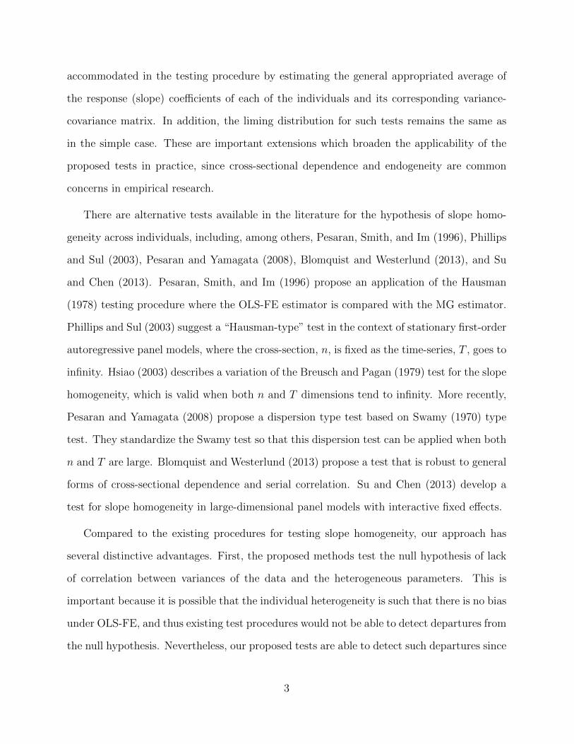
accommodated in the testing procedure by estimating the general appropriated average of

the response (slope) coefficients of each of the individuals and its corresponding variance-

covariance matrix. In addition, the liming distribution for such tests remains the same as

in the simple case. These are important extensions which broaden the applicability of the

proposed tests in practice, since cross-sectional dependence and endogeneity are common

concerns in empirical research.

There are alternative tests available in the literature for the hypothesis of slope homo-

geneity across individuals, including, among others, Pesaran, Smith, and Im (1996), Phillips

and Sul (2003), Pesaran and Yamagata (2008), Blomquist and Westerlund (2013), and Su

and Chen (2013). Pesaran, Smith, and Im (1996) propose an application of the Hausman

(1978) testing procedure where the OLS-FE estimator is compared with the MG estimator.

Phillips and Sul (2003) suggest a “Hausman-type” test in the context of stationary first-order

autoregressive panel models, where the cross-section, n, is fixed as the time-series, T , goes to

infinity. Hsiao (2003) describes a variation of the Breusch and Pagan (1979) test for the slope

homogeneity, which is valid when both n and T dimensions tend to infinity. More recently,

Pesaran and Yamagata (2008) propose a dispersion type test based on Swamy (1970) type

test. They standardize the Swamy test so that this dispersion test can be applied when both

n and T are large. Blomquist and Westerlund (2013) propose a test that is robust to general

forms of cross-sectional dependence and serial correlation. Su and Chen (2013) develop a

test for slope homogeneity in large-dimensional panel models with interactive fixed effects.

Compared to the existing procedures for testing slope homogeneity, our approach has

several distinctive advantages. First, the proposed methods test the null hypothesis of lack

of correlation between variances of the data and the heterogeneous parameters. This is

important because it is possible that the individual heterogeneity is such that there is no bias

under OLS-FE, and thus existing test procedures would not be able to detect departures from

the null hypothesis. Nevertheless, our proposed tests are able to detect such departures since

3

the tests are based on the correlation between variances of the data and the heterogeneous

parameters. Second, in the simplest case of the model, the tests do not require the time-series

to diverge to infinity. Third, the test procedures can be extended to accommodate correlation

between errors from different cross-sectional units, as well as a form of endogeneity. This

makes the testing procedure beneficial for many empirical applications.

Monte Carlo simulations assess the finite sample properties of the proposed methods.

The experiments suggest that the proposed approaches perform very well in finite samples.

The bias of fixed effects estimation can be made arbitrarily large by increasing the magnitude

of the covariance between the regression slope and the data variance. Critically, the MG

estimator we employ is unaffected by the slope heterogeneity bias. Finally, the new tests

possess good finite sample performance and have correct empirical size and power to detect

precisely the cases where OLS-FE is biased.

To illustrate the performance of the proposed methods in real-world data, we study em-

pirically the investment model of Fazzari et al. (1988), where a firm’s investment is regressed

on a proxy for investment demand (Tobin’s Q) and cash flow. Using annual COMPUSTAT

data covering a four-decade window, we study slope heterogeneity in investment models con-

trasting estimates from alternative methodologies. The coefficients returned for Q under the

methods we consider are fairly comparable in magnitude and significance. Results are very

different, however, for the response of investment to cash flow. Indeed, our tests identify

pronounced firm response heterogeneity, and the MG-estimated cash flow coefficient is sub-

stantially larger than those returned by the other methods. In concrete terms, the estimated

coefficient on cash flow increases from 0.057 (0.043) under the OLS (OLS-FE) estimation to

0.291 under the MG estimation; a 6–7-fold increase on the same data. For long panels, the

cash flow coefficient is 15 times larger under the MG method. Our results imply that cash

flow is a much more relevant driver of investment than previous studies have suggested.

The remainder of the paper is organized as follows. Section 2 describes the biases that

4

affect OLS-FE in the presence of individual slope heterogeneity, and discusses the MG es-

timator. Section 3 presents the proposed test for slope heterogeneity and its generalization.

Monte Carlo experiments are discussed in Section 4. In Section 5, we estimate a corporate

investment model and compare results from different methods. Section 6 concludes.

2 Understanding The Individual Heterogeneity Bias

This section presents the panel data model and characterizes the bias in the OLS-FE estima-

tor when the true econometric model allows for heterogeneous slope coefficients. To guide

researchers in their choice of methodology, we also show conditions under which the OLS-FE

returns consistent estimates. These conditions are limiting and imply potentially important

compromises for researchers’ inferences. We also discuss the mean group estimator.

2.1 Biases In The Individual-Fixed Effects Estimator

When modeling economic behavior, empiricists commonly estimate regression models that

allow individuals or firms to have different individual-fixed effects (different “intercepts”),

yet impose equal “slope” coefficients across units. As we show next, an incorrect homogenous

slope restriction leads to a bias in the policy estimates one obtains under the ordinary least

squares fixed effects (OLS-FE) framework.

Assume the following baseline model for the data generating process

yit = αi + x>itβi + uit, i = 1, ..., N, t = 1, ..., T, (1)

where yit is the dependent variable, xit is a k × 1 vector of exogenous regressors, and uit is

the conditionally mean zero innovation term. The term αi captures individual-specific fixed

effects, while the slope coefficients βi may vary across individuals.

5

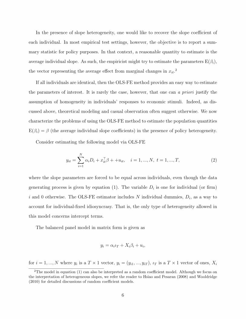
In the presence of slope heterogeneity, one would like to recover the slope coefficient of

each individual. In most empirical test settings, however, the objective is to report a sum-

mary statistic for policy purposes. In that context, a reasonable quantity to estimate is the

average individual slope. As such, the empiricist might try to estimate the parameters E(βi),

the vector representing the average effect from marginal changes in xit.2

If all individuals are identical, then the OLS-FE method provides an easy way to estimate

the parameters of interest. It is rarely the case, however, that one can a priori justify the

assumption of homogeneity in individuals’ responses to economic stimuli. Indeed, as dis-

cussed above, theoretical modeling and casual observation often suggest otherwise. We now

characterize the problems of using the OLS-FE method to estimate the population quantities

E(βi) = β (the average individual slope coefficients) in the presence of policy heterogeneity.

Consider estimating the following model via OLS-FE

yit =N∑i=1

αiDi + x>itβ + +uit, i = 1, ..., N, t = 1, ..., T, (2)

where the slope parameters are forced to be equal across individuals, even though the data

generating process is given by equation (1). The variable Di is one for individual (or firm)

i and 0 otherwise. The OLS-FE estimator includes N individual dummies, Di, as a way to

account for individual-fixed idiosyncrasy. That is, the only type of heterogeneity allowed in

this model concerns intercept terms.

The balanced panel model in matrix form is given as

yi = αiιT +Xiβi + ui,

for i = 1, ..., N where yi is a T × 1 vector, yi = (yi1, ..., yiT ), ιT is a T × 1 vector of ones, Xi

2The model in equation (1) can also be interpreted as a random coefficient model. Although we focus onthe interpretation of heterogeneous slopes, we refer the reader to Hsiao and Pesaran (2008) and Wooldridge(2010) for detailed discussions of random coefficient models.

6

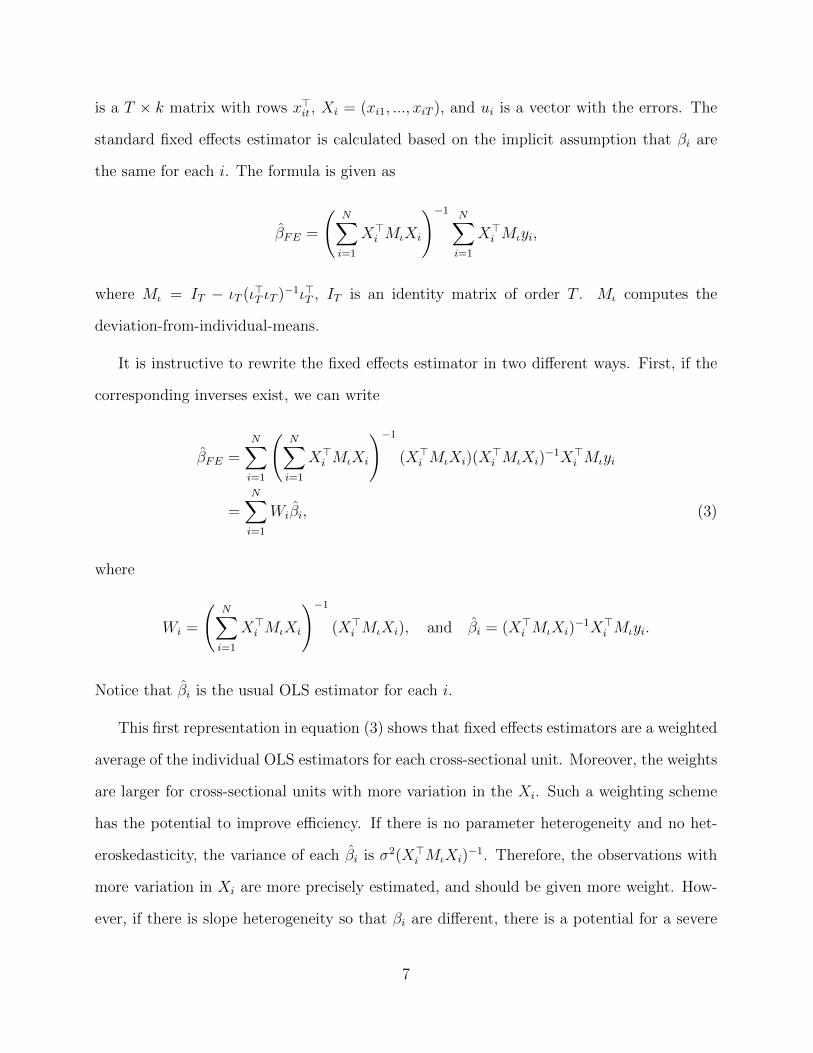
is a T × k matrix with rows x>it , Xi = (xi1, ..., xiT ), and ui is a vector with the errors. The

standard fixed effects estimator is calculated based on the implicit assumption that βi are

the same for each i. The formula is given as

βFE =

(N∑i=1

X>i MιXi

)−1 N∑i=1

X>i Mιyi,

where Mι = IT − ιT (ι>T ιT )−1ι>T , IT is an identity matrix of order T . Mι computes the

deviation-from-individual-means.

It is instructive to rewrite the fixed effects estimator in two different ways. First, if the

corresponding inverses exist, we can write

βFE =N∑i=1

(N∑i=1

X>i MιXi

)−1(X>i MιXi)(X

>i MιXi)

−1X>i Mιyi

=N∑i=1

Wiβi, (3)

where

Wi =

(N∑i=1

X>i MιXi

)−1(X>i MιXi), and βi = (X>i MιXi)

−1X>i Mιyi.

Notice that βi is the usual OLS estimator for each i.

This first representation in equation (3) shows that fixed effects estimators are a weighted

average of the individual OLS estimators for each cross-sectional unit. Moreover, the weights

are larger for cross-sectional units with more variation in the Xi. Such a weighting scheme

has the potential to improve efficiency. If there is no parameter heterogeneity and no het-

eroskedasticity, the variance of each βi is σ2(X>i MιXi)−1. Therefore, the observations with

more variation in Xi are more precisely estimated, and should be given more weight. How-

ever, if there is slope heterogeneity so that βi are different, there is a potential for a severe

7

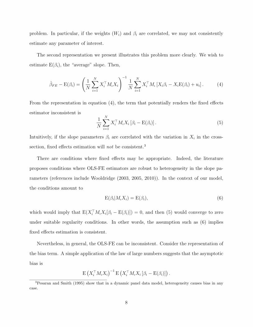
problem. In particular, if the weights (Wi) and βi are correlated, we may not consistently

estimate any parameter of interest.

The second representation we present illustrates this problem more clearly. We wish to

estimate E(βi), the “average” slope. Then,

βFE − E(βi) =

(1

N

N∑i=1

X>i MιXi

)−11

N

N∑i=1

X>i Mι [Xiβi −XiE(βi) + ui] . (4)

From the representation in equation (4), the term that potentially renders the fixed effects

estimator inconsistent is

1

N

N∑i=1

X>i MιXi [βi − E(βi)] . (5)

Intuitively, if the slope parameters βi are correlated with the variation in Xi in the cross-

section, fixed effects estimation will not be consistent.3

There are conditions where fixed effects may be appropriate. Indeed, the literature

proposes conditions where OLS-FE estimators are robust to heterogeneity in the slope pa-

rameters (references include Wooldridge (2003, 2005, 2010)). In the context of our model,

the conditions amount to

E(βi|MιXi) = E(βi), (6)

which would imply that E(X>i MιXi[βi − E(βi)]) = 0, and then (5) would converge to zero

under suitable regularity conditions. In other words, the assumption such as (6) implies

fixed effects estimation is consistent.

Nevertheless, in general, the OLS-FE can be inconsistent. Consider the representation of

the bias term. A simple application of the law of large numbers suggests that the asymptotic

bias is

E(X>i MιXi

)−1E(X>i MιXi [βi − E(βi)]

).

3Pesaran and Smith (1995) show that in a dynamic panel data model, heterogeneity causes bias in anycase.

8

To illustrate how this might arise in a simple empirical model, consider the standard linear

model with two covariates,

yit = αi + witθi + zitγi + uit.

The representation of the asymptotic bias for the simple model with two covariates is given

by following equation

θFE − E(θi)

γFE − E(γi)

p→

E(σ2wi) E(σwzi)

E(σwzi) E(σ2zi)

−1E[σ2

wi(θi − θ)] + E[σwzi(γi − γ)]

E[σwzi(θi − θ)] + E[σ2zi(γi − γ)]

, (7)

where σ2wi and σ2

zi represent the individual-specific variance of wit and zit, respectively, and

σwzi is the individual-specific covariance of wit and zit. What we see from the representation

in (7) is that, in general, the covariance between the variance of the regressors and the

parameters causes the bias. For example, if cross-sectional units with a high variance in

zit have a larger response measured by γi, there will be a positive asymptotic bias in the

fixed effects estimator for γ. Moreover, these effects can disseminate to the other parameter,

depending on the covariance structure. Nevertheless, equation (7) also shows that the OLS-

FE can be asymptotically unbiased when there is no covariance between the variance of the

regressors and the parameters. In this case, the elements in the vector in the far right-hand-

side are equal to zero.

2.2 The Mean Group Estimator: Estimation and Inference

Our focus is the estimation of models in which response parameters may vary across indi-

viduals observed over time (panel data). If response heterogeneity is part of the structural

model, one needs to decide what to report. In principle, one needs an estimator that is

useful in summarizing heterogeneity in the coefficients of interest, and that at the same time

is easy to compute and interpret. In this context, a measure of centrality of the distribution

9

of individuals’ responses is arguably a reasonable quantity to estimate.

The mean group (MG) estimator reports the mean of the regression slope parameters

as a way to summarize the population.4 For most applications in economics and finance,

a viable MG estimator will consist of the average of OLS coefficients from each individual

whose data are used to fit an empirical model. This can be represented by

βMG =1

N

N∑i=1

βi, (8)

where βi is the OLS for each sample individual.

The MG estimator allows for both the intercept and slope coefficients to vary across

individuals. This happens because, by applying OLS to each individual equation, one simul-

taneously estimate intercept (standard “fixed effects”) as well as slope coefficients for each

individual. Critically, the MG estimator does not suffer from the heterogeneity bias that

we characterize in the previous section. That the MG estimator is unbiased stems from the

fact that we fit the empirical model onto each individual separately, correctly accounting for

individual heterogeneity. The method combines individual estimates equally, averaging over

consistent parameters.

The interpretation of the estimator in (8) is straightforward. The population parameter

of interest is the mean coefficient over the sample individuals; βMG = E(βi). The estimator

βMG is the sample mean of individual slope estimates. In model (1) we can average over the

sensitivity of the dependent variable yit with respect to a covariate wit, holding zit constant.

From equation (1) the interpretation θi is

∂E(yit|xit, αi)∂xit

= βi.

4This estimator is fully developed in Pesaran (2006) and belongs to the class of minimum distanceestimators (see Newey and McFadden (1994)).

10

Similar to standard regression analysis, the MG estimator can be interpreted as the average

sensitivity of yit to xit, and E[ ∂E(yit|xit,αi)

∂xit

]= θMG.

Inference for the MG estimator is also straightforward. The asymptotic variance for√N(βMG − β) is estimated via

ΩMG =1

N − 1

N∑i=1

(βi − βMG)(βi − βMG)>. (9)

Inference is based on asymptotic normality as the time observations, T , and the number of

individuals, N , increase.

3 Testing Slope Heterogeneity

It is important that we present a practical procedure to identify and quantify problem of

slope heterogeneity. In this section, we first review a test for the presence of slope hetero-

geneity building on dispersion tests by Pesaran and Yamagata (2008) and Swamy (1970).

Importantly, as noted in Section 2, it is possible that the individual heterogeneity is such

that there is no bias under the OLS-FE. Thus, second, we propose a novel test designed to

detect precisely when and how slope heterogeneity will cause bias in parameters estimated

via OLS-FE. Third, we generalized the proposed test to allow for cross-sectional dependence

in the errors and in the regressors, and also a form of endogeneity.

3.1 Identifying Slope Heterogeneity

Pesaran and Yamagata (2008) consider the regression panel model with N individuals and T

time periods in equation (1). Let βi be the vector of policy parameters in the model, k × 1.

11

We wish to test the following null hypothesis of slope homogeneity across individuals

H0 : βi = β,

for some fixed vector β for all i, against the alternative

H1 : βi 6= βj for some i, j.

The strategy is to estimate regression coefficients using the time-series for each individual,

then compare the estimates with β. Under the null, the estimates for each individual should

be close to β. Large differences across these estimates and β indicate that the null should

be rejected. Since we do not observe the true coefficient β, we replace it with βWFE, which

is a weighted version of the fixed effects estimator.

The test is defined as

S :=N∑i=1

(βi − βWFE

)>(X>i MιXi

σ2i

)−1 (βi − βWFE

),

where σ2i = (yi−XiβFE)>Mι(yi−XiβFE)

(T−k−1) , βFE is the standard OLS-FE, and βWFE is defined as

βWFE =(∑N

i=1X>i MιXiσ2i

)−1∑Ni=1

X>i Mιyiσ2i

. One can also consider a standardized version of the

test as ∆ =√N

1NS−k√2k

. Under standard regularity conditions (see Pesaran and Yamagata

(2008)):

Sd→ χ2

(N−1)k, as T →∞;

∆d→ N(0, 1), as (N, T )→∞.

where k is the number of restriction under the null hypothesis.

12

3.2 Diagnosing The Bias In The Fixed Effects Estimator

The Pesaran-Yamagata-Swamy (PYS) test presented above provides a way to identify the

presence of individual slope heterogeneity in a model. Slope heterogeneity, however, need

not cause OLS-FE estimates to be biased as shown in equation (7) (see also Wooldridge

(2005, 2010)). Alternatively, the bias could be small enough so as to make the OLS-FE still

desirable. We now introduce a novel test measuring the magnitude of the slope heterogene-

ity bias in OLS-FE estimations. In the next section, we generalize the test to accommodate

more general conditions and allow for cross-sectional dependence in the errors and in the

regressors, as well as a form of endogeneity.

We wish to test the hypothesis that the heterogeneity across individuals does not in-

duce a bias in the OLS-FE estimator. Equation (7) shows that the OLS-FE estimates are

asymptotically biased when the heterogeneous coefficients are related to the variance and

covariance of the regressors. Thus, we construct a test based on this result. In particular,

we wish to test the null hypothesis that there is no correlation between the coefficients and

covariance of the regressors. Formally, the null hypothesis is define as

H0 : E[X>i MιXi(βi − β)

]= 0, (10)

where Xi = (xi1, ..., xiT ). The test statistic for the null hypothesis in (10) is based on an

estimate of equation (5). Define

δ =1

N

N∑i=1

X>i MιXi(βi − βMG)

=1

N

N∑i=1

δi.

The term δ is an estimate of the quantity that causes the OLS-FE to be inconsistent. We

want to test if that quantity is significantly different from zero. To this end, we need an

13

estimate of its variance, which is calculated using

Ω =1

N

N∑i=1

δiδ>i .

The statistic of interest, which we refer to as the heterogeneity bias (HB) test, is given by

HB = N × δ>Ω+δ, (11)

where Ω+ is the Moore-Penrose inverse of Ω.

The null hypothesis is that heterogeneity in slope parameters does not cause OLS-FE to

be inconsistent. Rejection of the null implies that one should use the MG estimator instead.

Remark 3.1 Hsiao and Pesaran (2008) propose an alternative Hausman test for slope het-

erogeneity. In particular, they test the difference between the Mean Group estimator and a

pooled estimator (like fixed effects). However, in their framework, under the null of no het-

erogeneity in slopes (nor in error variances), fixed effects is an efficient estimator. Hence,

they are able to apply the usual Hausman type variance estimator (the difference between

the consistent estimator and efficient estimator variances) to standardize the statistic. In

our setup, we do not impose lack of heterogeneity under the null, only a population moment

condition as in (10) where fixed effects is consistent. Rejection of the Hausman test might

be due to slope heterogeneity, slope heterogeneity bias of fixed effects, or lack of efficiency of

the fixed effects estimator for a given empirical situation. Our test is designed to target only

the potential bias of fixed effects estimation.

Next, we derive the limiting distribution of the proposed HB test. To this end, we

consider the following set of assumptions.

Assumption 1 Let the matrix Xi have rows x>it . Suppose that for all i, T−1(XiMιXi) is

invertible.

14

Assumption 2 The terms T−1(X>i MιXi)(βi− β) are independent across i with finite vari-

ance.

Assumption 3 Errors ui are independent across i with E(ui|Xj, αj) = 0 for all i and j,

and uj is independent of βi for all i and j.

Assumption 1 allows us to estimate each individual slope parameter, βi. This assumption

could be violated for cases with a limited number of time-series observations, T , for example.

It is important to notice that, Condition 1 does not explicitly require T → ∞, which is

a common requirement in the literature (see, e.g., Phillips and Sul (2003), Pesaran and

Yamagata (2008), Su and Chen (2013)), but it requires enough variability in the time-series

dimension to be satisfied. Assumption 2 is related to the usual assumption in random

coefficient models where the parameters are all assumed to be independent of each other

as well as independent of the data (see, e.g., Hsiao (2003)) for a discussion. Assumption 3

is similar to the standard assumption restricting the errors on the cross-section dimension

when T is finite (such as Wooldridge (2010)). Note that the assumptions allow for serially

correlated errors as well as heterosekasticity. Assumptions 1–3 are very mild and standard

in the literature. Nevertheless, below we will relax these assumptions and modify our test

to accommodate the more general conditions.

Now we present the asymptotic distributions of the HB test.

Theorem 1 Suppose that Assumptions 1-3 hold and that H0 : E[X>i MιXi(βi − β)

]= 0,

then as N →∞ with T finite,

Nδ>Ω+δd→ χ2

k,

where k is the number of regressors in the model.

Proof. In Appendix A.

15

Theorem 1 provides the asymptotic distribution of new test. Notably, implementation of

the proposed heterogeneity test is straightforward. One simply: (I) computes the test statis-

tic, HB, using in equation (11); (II) sets the level of significance; and (III) finds the critical

values from standard distribution tables. Since HB is asymptotically bounded by a chi-

square distribution, critical values are tabulated and widely available. The null hypothesis is

rejected if the value of the test is outside the interval defined by the critical value of choice.

It is important to highlight the differences between the HB and PYS tests. The HB test

is designed to test a completely different null hypothesis. In particular, the null hypothesis

associated with the HB test is the lack of correlation between variances of the data and the

heterogeneous parameters. The PYS test takes the null hypothesis of no parameter hetero-

geneity, and detects heterogeneity. Therefore, it is possible to reject the null of parameter

heterogeneity with the PYS test, yet fail to reject the null of no bias in the fixed effects

estimator. The tests are very much complementary.

3.3 Cross-Sectional Dependence

The results presented in the paper can be extended to more general cases. In particular, we

can allow for correlation between errors from different cross-sectional units, and a form of

endogeneity. In this subsection we show that these extensions can be easily accommodated in

the testing procedure by estimating the general appropriated average of the response (slope)

coefficients of each of the individuals and its corresponding variance-covariance matrix.

In particular, consider the following model

yit = αi + x>itβi + uit,

uit = φ>i ft + εit,

where each φi is 1× j and ft is a j × 1 vector of unobserved factors.

16

In the above model, the presence of ft allow us to consider cross-section dependence in

the errors and in the regressors, and also a form of endogeneity. First, the existence of ft

in each of the cross-sectional equations allows for cross-sectional dependence in the uit error

terms. Such dependence is modeled in Bai (2009) and Pesaran (2006), among others. In

addition to allowing for cross-sectional dependence between the errors, explicit dependence

between the factors and the covariates is allowed via

xit = ηi + Λ>i ft + vit.

Hence, second, ft allows for dependence between cross-sectional covariates. That is, xit and

xjt are dependent through the mutual presence of ft. Third, the more general model uses ft

in the dual roles of cross-sectional dependence of error terms, as well as endogeneity of xit

through the effects of ft on both uit and xit.

Pesaran (2006) shows that the average parameter E(βi) can be consistently estimated by

including the cross-sectional averages at each time period, y·t and x·t, in each unit regression,

and combining via the sample average. To see this, write the model as a system,

yitxit

=

αi + β>i ηi

ηi

+

β>i Λ>i + φ>i

Λ>i

ft +

β>i vit + εit

vit

= Bi + C>i ft + ξit.

17

The factors, ft can be estimated using this model. Define

y·t =1

N

N∑i=1

yit, x·t =1

N

N∑i=1

xit,

ξ·t =1

N

N∑i=1

ξit, B =1

N

N∑i=1

Bi,

C =1

N

N∑i=1

Ci.

If the rank of C is full for all N , then we can solve for ft as

ft = (CC>)−1C

y·tx·t

− B − ξ·t .

The model for yit is written as

yit = αi + x>itβi + φ>i (CC>)−1C

y·tx·t

− B − ξ·t+ εit.

Under regularity conditions, ξ·t will converge to zero, and hence we can use y·t and x·t in the

model to account for ft. For each cross-sectional unit, we can estimate βi, and then consider

the mean group estimator accounting for cross-sectional correlation. To this end, define the

T × (k + 2) matrix

Q =

1 y·1 x>·1...

......

1 y·T x>·T

,

18

and let MQ = I −Q(Q>Q)+Q>, so that

βCi = (X>i MQXi)−1X>i MQyi.

The goal of using the cross-sectional averages as regressors is to approximate the factors, ft.

If the factors were actually observed, we could replace MQ with MG where we define

G =

1 f>1...

...

1 f>T

.

This matrix will be important for the asymptotic results, and we will include an assumption

about this matrix in what follows.

The analogue of the fixed effects estimator when allowing for cross-sectional dependence

and endogeneity is given by the pooled estimator of Pesaran (2006)

βP =

(N∑i=1

X>i MQXi

)−1 N∑i=1

X>i MQyi,

where efficiency gains are possible if there is no heterogeneity of the βi parameters. Therefore,

the analogue of the Mean Group estimator, which we label Mean Group Correlated (MGC)

is given as

βMGC =1

N

N∑i

βCi.

The βMGC is used in the construction of the general version of the HB test. Similar to

19

the construction of the test above, we have

δC =1

N

N∑i=1

X>i MQXi(βCi − βMGC) (12)

=1

N

N∑i=1

δci.

Finally, to obtain the statistic of test we need the corresponding variance-covariance matrix,

which is computed as

ΩC =1

N − 1

N∑i=1

δCiδ>Ci.

Therefore, analogously to the previous test case, we wish to test the hypothesis that

the heterogeneity across individuals does not induce a bias in the pooled estimator (βP ).

These estimates are asymptotically biased when the heterogeneous coefficients are related

to the variance and covariance of the regressors. As in previous section, we wish to test the

null hypothesis that there is no correlation between the coefficients and covariance of the

regressors. The null hypothesis is define as

H0 : E[(X>i MGXi)(βi − β)

]= 0. (13)

The test statistic for the null hypothesis in (13) will be based on an estimate of equation

(12).

We refer to the modified test as the Heterogeneity Bias Cross test (HBC) as it allows

for the cross-sectional dependence and endogeneity through the factor structure. The test

statistic is defined as following

HBC = Nδ>C Ω+C δC . (14)

The presence of the factors ft changes the assumptions needed to obtain the same limiting

distribution, and are similar to those of Pesaran (2006). We consider the following set of

20

assumptions.

Assumption 4 The common factors ft are covariance stationary with absolutely summable

autocovariances. Moreover, ft is independent of εit′ and vit′ for all i, t, t′.

Assumption 5 The variables εit and vit are independently distributed for all i, j, t, t′. Both

εit and vit are linear stationary processes with absolutely summable autocovariances, where

the error process has finite fourth order cumulants.

Assumption 6 The factor loadings φi and λi are iid and independent of all ft, εjt, vjt

textcolorredfor all i, j, t. φi and λi have finite second moment matrices.

Assumption 7 The βi are iid and independent of all ft, εjt, φj and λj for all i, j, t. The

terms β>i vit are independent across i with mean zero and finite fourth order cumulants.

Assumption 8 The matrices T−1(X>i MQXi) and T−1(X>i MGXi) are non-singular for all

i, and their respective inverses have finite second-order moment matrices for all i.

Assumption 9 T−1(X>i MGXi)(βi − β) are independent across i with finite second-order

moment matrices.

Assumption 10 The matrix C is full rank j ≤ (k + 1) for all N .

These assumptions are general and allow for a wide variety of data generating processes.

Assumption 4 restricts the dependence between the cross-sectional xit variables to be solely

a function of the factors, while Assumption 6 ensures that the factors and the other error

processes do not influence the loadings. Assumption 5 is a standard condition on stationar-

ity of the innovation terms only requiring the corresponding fourth comments to be finite.

Assumption 7 restricts the dependence between βi and the other variables.5 Assumption 8

5This assumption is a modification of Assumption 4 of Pesaran (2006) in that we allow for βi to becorrelated with the variance of vit, as will happen when fixed effects is not consistent.

21

is an identification condition for each of the cross-sectional units. The independence condi-

tion from Assumption 9 is more general than it might first appear. The Xi matrices might

themselves be dependent across i due to the factor structure. However, MG matrix will

eliminate the factors, so that we are essentially restricting the dependence of βi between

cross-sectional units. Assumption 10 is the rank condition for identification of ft. Pesaran

(2006) shows that the mean group estimator is still consistent if this assumption does not

hold. We conjecture that our results would also hold if this assumption does not hold, but

with a modification of Assumption 9.

The next result presents the asymptotic distribution of the HBC test.

Theorem 2 Suppose that Assumptions 4-10 hold and that H0 : E[T−1(X>i MGXi)(βi − β)

]=

0. Then as (N, T )→∞,

Nδ>C Ω+C δC → χ2

q,

where q ≤ k, with q the rank of E[T−2(X>i MGXi)(βi − β)(βi − β)>(X>i MGXi)

].

Proof. In Appendix B.

Notice that if we fail to reject the null hypothesis, then it may be appropriate to use the

pooled estimator. The limiting distribution of the test in Theorem 2 is different from than

in Theorem 1 for two reasons. First, for the HBC we require T → ∞ to apply the central

limit theorem to δC . Second, ΩC converges to

E[T−2(X>i MGXi)(βi − β)(βi − β)>(X>i MGXi)

].

The rank of this matrix may vary from 0 to k. For example, in the extreme case where there

is no heterogeneity, βi = β for each i, and the rank is 0. The statistic would converge to 0, so

that critical values for a χ2k would be conservative. Of course, we would correctly fail to reject

that null hypothesis that heterogeneity does not cause bias, as there is no heterogeneity.

22

To summarize, practical implementation of the test is straightforward. The test is com-

puted in a similar way to the HB test, but with the addition of cross-sectional averages in

the regressions for each unit. One compares the HBC statistic to a χ2k distribution. The test

will reject the null as there is more heterogeneity bias. In addition, the test correctly becomes

more conservative if there are fewer parameters in the model that exhibit heterogeneity.

4 Monte Carlo

We use Monte Carlo simulations to assess the performance of the methods discussed in the

previous sections. Our simulations allow for varying degrees of importance assigned to in-

dividual slope heterogeneity. The main objective is to assess the finite sample performance

of the HB and HBC tests. We evaluate them in terms of size and power. We also compare

the standard OLS (without fixed effects), OLS-FE, MG, and MGC estimators in terms of

inferential bias and efficiency. Our goal is to illustrate the importance of the individual het-

erogeneity bias, and its impact on different estimation methods under various data scenarios.

In doing so, we restrict our attention to the following cases: (1) no heterogeneity bias; (2)

heterogeneity affecting one regressor; (3) heterogeneity affecting both regressors. The first

case illustrates the case in which OLS-FE is unbiased and gives the size of the tests. The

second case shows that one coefficient can be biased while the other remains unbiased. The

last case is more general, as both coefficients can be biased. The last two cases provide the

power of the tests.

4.1 Monte Carlo Designs

We consider a simple data generating process (DGP). The variable yit is generated by the

model

yit = αi + θiwit + γizit + uit, (15)

23

where αi is the individual-specific intercept term, while θi and γi are individual-specific slope

coefficients associated with exogenous variables wit and zit, respectively. The regression error

term, uit, is normally distributed with mean zero and variance one.

As discussed in Section 2, fixed effects estimation of the population averages E(θi) and

E(γi) will be biased if there is a non-zero covariance between θi and the variance of wit, or

if there is non-zero covariance between γi and the variance of zit. We model the dependence

in zit and γi, and the heterogeneity in γi as follows:

zit = αi + εzit and wit = 1 + εwit,

where

εzit ∼ N(0, σ2zi), ε

wit ∼ N(0, σ2

wi); σ2zi = 1 + vzi, σ

2wi = 1 + vwi; vwi ∼ vzi ∼ χ2

1;

αi ∼ N(0, 1), uit ∼ N(0, 1).

We divide our experiments into three parts. In the first two parts main objective is to in-

vestigate the finite sample performance of the HB test, and in the third part we assess the

HBC test.6

In the first part, we set θi = 1 for all individuals in order to isolate the effect of just

one of the variables having a heterogeneous effect on yit. The parameter γi, representing the

individual-specific slope, is generated as

γi = 1 + 2c− cσ2zi + dεγi ,

where εγi is N(0, 1) and c = 0,±0.5,±1. The parameter d is given by d = (2 − 2c2)1/2 so

6We conducted other experiments where the errors were serially correlated. The results were similar andare available upon request.

24

that the variance of γi equals 2 regardless of the correlation between σ2zi and γi.

The experiments use the parameter c to modulate the importance of individual slope

heterogeneity. When c = 0, there is heterogeneity in γi coming from εγi . However, since

c = 0, the heterogeneity in the slope coefficient γi is not correlated with the variance in the

regressor zit, and the fixed effects estimator provides an unbiased estimate of E(γi). As c

increases in magnitude, the covariance between γi and σ2zi increases, leading to biases in the

fixed effects estimation of E(γi). For example, when c = 1, the covariance between γi and

σ2zi is –2, resulting in negative bias of the fixed effects estimator. Intuitively, the fixed effects

estimator assigns more weight to individuals that have smaller slope coefficients γi. When

c = −1, we have the opposite effect, and the fixed effects estimator will be positively biased.

Therefore, the parameter c is very important. Under the null hypothesis of slope homogeneity

c = 0, and we obtain the size of the HB test. Then, c 6= 0 we have slope heterogeneity that

causes bias in OLS-FE, and we are able to examine the power of the proposed HB test.

In the second part of the experiment, we also allow θi to be heterogeneous, and generated

by θi = 1 + 2c− cσ2wi + dεθi , where εθi ∼ N(0, 1). In this set of simulations, by controlling the

constant c, we are examining the size and power of the tests. Again, when c = 0 we recover

size, when c 6= 0 we have power of the tests.

Finally, in the third part, we explore size and power of the HBC test by allowing for

a factor structure to generate cross-sectional dependence in the errors and endogeneity. In

particular, we use the DGP model as in equation (15). In this case, we maintain the same

format as in the first case and set θi = 1 for all individuals. The covariate zit has zit = αi+εzit

with εzit ∼ N(0, σ2zi), σ

2zi = 1 + vzi, vzi ∼ χ2

1. Nevertheless we introduce the structure of wit

generates cross-sectional dependence in the errors and endogeneity as follows

wit = 1 + λ>i ft + εwit, and uit = φ>i ft + εit,

λi = (1, 1)>, and φi = (1, 1)> + ξi,

25

where ft is a 2 × 1 vector of iid standard normal variables, and ξi is a 2 × 1 vector of iid

standard normal variables. The presence of the factor in the variable wit causes endogene-

ity between uit and wit. Finally, as in the first case, the parameter γi, representing the

indivual-specific slope, is generated as

γi = 1 + 2c− cσ2zi + dεγi ,

where εγi is N(0, 1) and c = 0,±0.5,±1, and the parameter d is given by d = (2 − 2c2)1/2.

Once again, the parameter c controls the size and the power of the test.

To benchmark our results, we estimate the model using traditional OLS, where all indi-

viduals are (incorrectly) assumed to have the same intercept and slopes. Under the data gen-

erating process above, the OLS estimate of E(γi) will be biased since the individual-specific

intercept terms are correlated with zit, and OLS is unable to account for individual effects

and cross-sectional slope heterogeneity. We also report results for the OLS-FE model that

allows for individual intercepts, but as is standard, assumes that the slopes are homogeneous.

Finally, we include the mean group estimators. The MG is presented for all comparisons, it

allows for individual-specific intercepts as well as slope coefficients. The MGC is presented

for the third part of the exercise, and it allows for the cross-sectional dependence.

4.2 Monte Carlo Results

We examine the finite sample properties of the methods considering different DGP. We use

N = 500 for the number of individuals and set the number of time observations, T , alterna-

tively, to 5, 10, 20, and 30. The number of replications in each experiment is 5,000.7 We first

report the results for evaluation of the estimators. Then, we describe the results for the tests.

7Since the data used in many empirical applications face limitations on the times series dimension, T,our main presentation focuses on variations along this dimension. However, in unreported tables we alsoexperiment with variations in the number of individuals, N (e.g., N = 100 and N = 1,000). These alternativeexperiments lead to similar inferences and are readily available from the authors.

26

4.2.1 Results For Bias And RMSE

Results For Experimental Design 1

Table 1 reports the bias and RMSE associated with each of the estimators considered in

the first experimental design. In the absence of estimation biases, we would expect to find

E(θi) = 1 and E(γi) = 0. Deviations from these benchmarks measure the degree of bias in the

estimated coefficient. Estimators with better inference properties should present low RMSEs.

Table 1 About Here

As predicted, the OLS estimator is biased even when c = 0, and they produce similar re-

sults. For example, with T = 5 the bias for E(γi) under OLS is 0.334. As the time dimension,

T , increases, the OLS bias does not decline. In sharp contrast, the bias under OLS-FE and

MG is virtually zero; less than –0.001 in both cases. While the OLS-FE and MG estimators

have similar, negligible biases, the MG has the smallest RMSE. The reason that OLS-FE

does not have the smallest RMSE for the case of c = 0 is that it is not efficient even though

it is unbiased. The intuition is that if OLS is appropriate in a model with heterogeneity only

in intercepts, the random effects model is more efficient. Even though OLS-FE is consistent

(unbiased) when c = 0, it is not efficient. Moreover, MG has smaller variance for this case

even though its use is not necessary.

Now we allow for c 6= 0. When c = −0.5, the covariance between γi and σ2zi is positive

and we should see a positive bias in the OLS-FE estimator. This is what we see in Table 1.

The estimated values of E(γi) under OLS-FE are now positively biased with values 0.493,

0.496, 0.494, and 0.497 for T = 5, 10, 20, and 30, respectively. The bias is insensitive by in-

creases in the times series dimension. At the same time, the OLS estimate is still biased and

have the largest RMSEs. The MG estimator performs uniformly better than all of the other

estimators, both in terms of bias magnitude and RMSE. Indeed, the MG method produces

virtually unbiased estimates.

27

When c = 0.5, we see a negative bias in E(γi) for OLS-FE. In this case, the bias in OLS

is smaller than when c = −0.5, which is an artifact of conflicting bias directions from the

intercept effects, αi, and the slope effects, γi. A more interesting observation is that the sign

of the OLS-FE bias changes when c = 0.5. This change highlights the inferential instability

of the OLS-FE estimator in the presence of individual slope heterogeneity.

Finally, as we increase the magnitude of the correlation between γi and σ2zi via c = −1,

the bias for OLS-FE is approximately –1, while that of the MG remains virtually equal to

zero. That is, under this form of individual slope heterogeneity the OLS-FE suffers from

a severe attenuation-like bias that assigns no relevance to estimates associated with the af-

fected variable, even though the variable has a strong predictive power in the true economic

model. For c = 1, the sign of the OLS-FE bias changes, but the magnitudes are similar

to those found when c = −1. That is, estimates associated with the affected variable are

grossly overestimated and appear to be twice as important as they are in the true model.

Notably, the magnitudes of these biases are insensitive to T .

Results For Experimental Design 2

We now change the data generating process by also letting θi vary across individuals. This

new experiment allows one to have correlation between both slope parameters of the model

and the variance of the data. The results of these experiments appear in Table 2.

Table 2 About Here

When c = 0, by design, the variable wit is uncorrelated with the individual-specific in-

tercept, αi, so that E(θi) should be unbiased. The results in Table 2 confirm this prediction

and show approximately unbiased estimates for E(θi) for the OLS, OLS-FE, and MG esti-

mators. There is, however, a significant bias for E(γi) under OLS estimation, and this bias is

insensitive to the times series dimension. Finally, both OLS-FE and MG are approximately

28

unbiased for E(γi), with MG having the smallest RMSE.

As c increases in magnitude, the bias and RMSE are expected to increase for OLS, and

OLS-FE estimators. Table 2 confirms these predictions. The bias of the OLS-FE estimator

is significant for both slope coefficients, whereas MG is largely immune to biases, even for

short panels. In addition, the RMSE of the MG estimator declines as the time dimension of

the panels increases.

Results For Experimental Design 3

The results from the experiment with the factors is presented in Table 3.8 There are several

important points to note from this experiment. First, the parameter θi is not heterogeneous

in this experiment. However, it is the coefficient for the variable wit which is a function of

the factor ft. Hence, this variable is endogenous. Therefore, we see that OLS, FE, and MG

experience bias for each of the cases considered. The estimator that corrects for this effect,

MGC, is not affected. As the correlation between the variance of the regressors zit and the

parameter γi increases through c, both OLS and OLS-FE perform worse. Again, MGC is

unaffected by the correlation that causes heterogeneity bias.

Table 3 About Here

4.2.2 Depicting The Bias

As a complementary simulation exercise and to illustrate the size of the bias, we reproduce

the experiment for c between 0 and –1, graphing the bias of E(γi) as a function of the param-

eter c for the OLS, OLS-FE, and MG estimators. The results are plotted in Figure 1. One

can see that the MG estimator is unaffected by the correlation of the heterogeneous slope

parameter, γi, with the variance of the data, σ2zi. The other estimators are, in contrast, very

8The tests are not computed for T = 5 as there are not enough observations for each cross-sectionalregression when the additional cross-sectional means are added.

29

Figure 1: Heterogeneity bias

0.0 0.2 0.4 0.6 0.8 1.0-c

-0.1

0.1

0.3

0.5

0.7

0.9

Bia

s OLSOLS-FEMG

Figure 1 shows the bias of E(γi) for OLS, OLS-FE, and MG estimators as a function of the parameterc in the simulations, where c is between 0 and –1.

sensitive to heterogeneity in γi as it becomes more correlated with its regressor variance.

4.2.3 Results For The Heterogeneity Bias Test

We now explore the use of the HB and HBC tests in measuring the extent to which slope

heterogeneity causes OLS-FE estimates to be biased. We report the empirical size and power

of the tests. We use a 5% nominal size for all computations.

The Experimental designs 1 and 2 assess the finite sample performance of the HB test.

They produce equivalent results. Thus, we report results for the first only in Figure 2. The

results illustrate the costs of parameter heterogeneity. The HB test is applied to experi-

mental design 1 for N = 200, 500, and 1, 000, as well as values of T = 10, 20, and 30. When

c = 0 we obtain the size of the test. As the parameter c increases (in absolute values), there

is more bias from parameter heterogeneity. For each of the respective sample sizes, we plot

the percentage of rejections of the null hypothesis that OLS-FE estimates are unbiased for

5,000 replications.

30

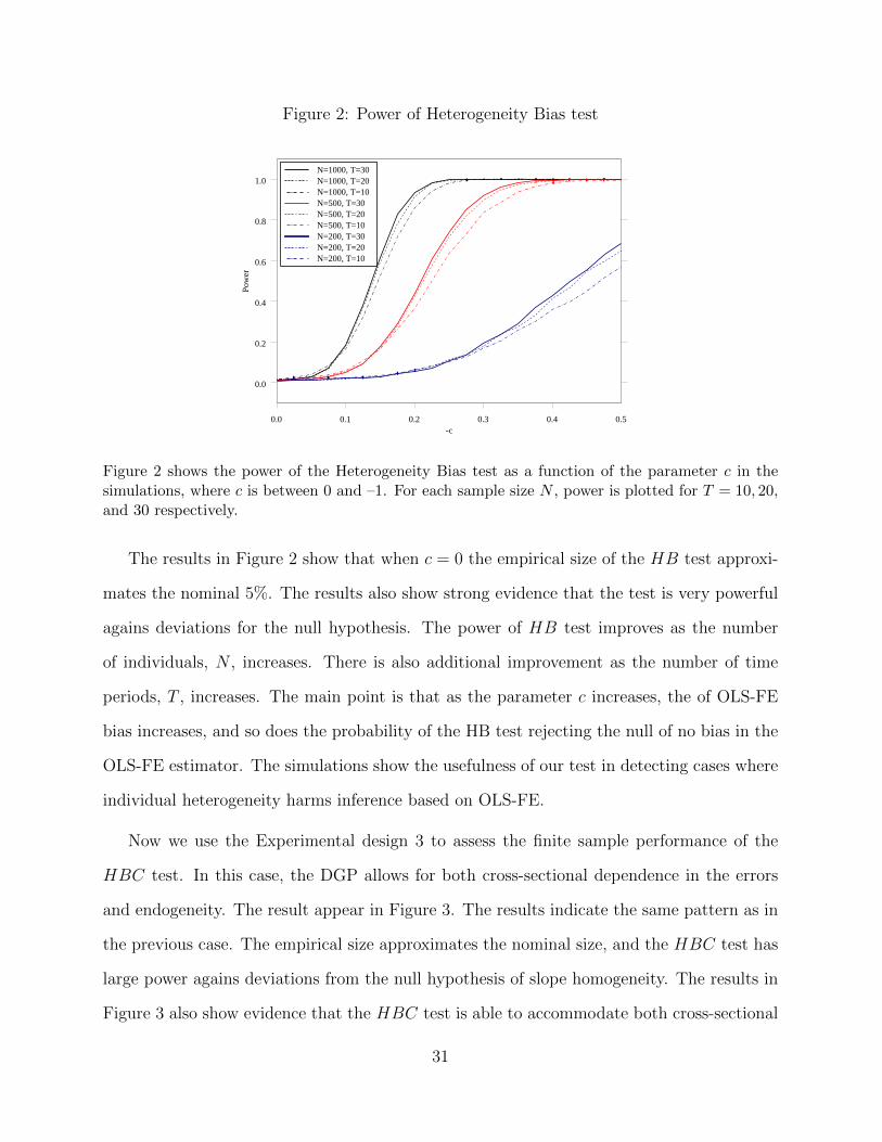
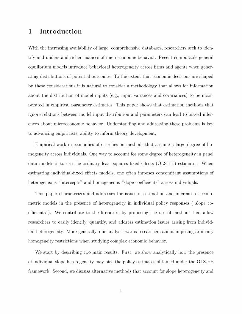
Figure 2: Power of Heterogeneity Bias test

0.0 0.1 0.2 0.3 0.4 0.5-c

0.0

0.2

0.4

0.6

0.8

1.0

Pow

er

N=1000, T=30N=1000, T=20N=1000, T=10N=500, T=30N=500, T=20N=500, T=10N=200, T=30N=200, T=20N=200, T=10

Figure 2 shows the power of the Heterogeneity Bias test as a function of the parameter c in thesimulations, where c is between 0 and –1. For each sample size N , power is plotted for T = 10, 20,and 30 respectively.

The results in Figure 2 show that when c = 0 the empirical size of the HB test approxi-

mates the nominal 5%. The results also show strong evidence that the test is very powerful

agains deviations for the null hypothesis. The power of HB test improves as the number

of individuals, N , increases. There is also additional improvement as the number of time

periods, T , increases. The main point is that as the parameter c increases, the of OLS-FE

bias increases, and so does the probability of the HB test rejecting the null of no bias in the

OLS-FE estimator. The simulations show the usefulness of our test in detecting cases where

individual heterogeneity harms inference based on OLS-FE.

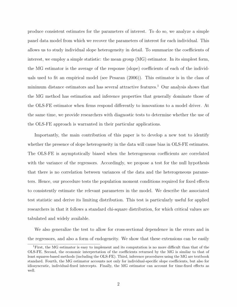
Now we use the Experimental design 3 to assess the finite sample performance of the

HBC test. In this case, the DGP allows for both cross-sectional dependence in the errors

and endogeneity. The result appear in Figure 3. The results indicate the same pattern as in

the previous case. The empirical size approximates the nominal size, and the HBC test has

large power agains deviations from the null hypothesis of slope homogeneity. The results in

Figure 3 also show evidence that the HBC test is able to accommodate both cross-sectional

31

Figure 3: Power of Heterogeneity Bias Cross test

0.0 0.1 0.2 0.3 0.4 0.5-c

0.0

0.2

0.4

0.6

0.8

1.0

Pow

er

N=200, T=10N=200, T=20N=200, T=30N=500, T=10N=500, T=20N=500, T=30N=1000, T=10N=1000, T=20N=1000, T=30

Figure 3 shows the power of the Heterogeneity Bias test as a function of the parameter c in thesimulations, where c is between 0 and –1. For each sample size N , power is plotted for T = 10, 20,and 30 respectively.

dependence in the errors and endogeneity without size distortion or power loss. This is due

to the fact that the test makes use of the proper point estimates and their corresponding

variance-covariance matrix.

To summarize our Monte Carlo experiments, we show that heterogeneity in individual

responses to a given economic driver may introduce severe biases in methods commonly

used to estimate policy parameters. Focusing on estimators designed to recover individuals’

average response (slope) coefficients, we find that the bias of fixed effects estimation can be

made arbitrarily large by increasing the magnitude of the covariance between the regression

slope and the data variance. The bias can be positive or negative depending on the sign of

the covariance. Critically, the mean group estimator we employ is unaffected by the slope

heterogeneity bias. In addition, the mean group estimator has the smallest RMSE (hence,

the best performance under this inference metric) over the range of our experiments. The

32

bias and RMSE for the MG estimator is uniformly smaller than those of the other estimators.

Moreover those statistics are largely insensitive to the time dimension, T . Finally, we show

that our new HB and HBC tests have correct empirical size and power to detect precisely

the cases where OLS-FE is biased. The HBC test is expected to perform well in empirical

setting since it is able to allow for both cross-sectional dependence and endogeneity.

5 Empirical Application: Investment Models

We illustrate our proposed techniques for estimating models with slope heterogeneity us-

ing a traditional corporate finance application. In particular, we compare OLS-FE, MG,

and MGC estimators in the context of the Fazzari et al.’s (1988) investment model. In the

model, a firm’s investment spending is regressed on a proxy for investment demand (Tobin’s

Q) and operating cash flows. A review of the corporate investment literature shows that

virtually all empirical work in the area considers panel data models with firm-fixed effects

(see, among others, Kaplan and Zingales (1997) and Rauh (2006)). At the same time that

there is a consensus about the inclusion of firm-specific intercepts, existing studies assume

homogeneous slope coefficients for Q and cash flow across individual firms.9

The Fazzari et al. model is commonly represented as

Investmentit = αi + θQit + γCash F lowit + uit, (16)

where Investment is the ratio of current investment spending scaled by the firm’s lagged

capital stock, Q is the ratio of the firm’s market value over the book value of assets, and

Cash F low is the firm’s operating income divided by its lagged capital stock. The parameter

αi is the firm-specific fixed effect and uit is the innovation term.

9A number of papers estimate investment–cash flow sensitivities for sample partitions based on proxiesfor financial constraints (e.g., firm size or existence of bond ratings). These estimations are also subject tothe firm heterogeneity biases that we highlight in our paper.

33

Suppose that investment is governed by

Investmentit = αi + θiQit + γiCash F lowit + uit, (17)

with θi and γi possibly different across firms. When data is generated according equation

(17), assuming an homogeneous θ and γ across a panel of firms and estimating model (16)

may result in severely biased parameters and incorrect inferences. In what follows, we con-

cretely characterize the problems that arise from estimating (16) in lieu of (17).

5.1 Data Description

Our data are taken from COMPUSTAT from 1970 through 2010. The sample consists of

manufacturing firms with fixed capital of more than $5 million (with 1976 as the base year

for the CPI). We only study firms whose annual assets and sales growth are less than 100%

(e.g., Almeida and Campello (2007)). Summary statistics for investment, Q, and cash flow

are presented in Table 4. Since these statistics are similar to those found in other studies,

we omit a discussion of their properties.

Table 4 About Here

To assess the performance of different estimators over the times series dimension, we

classify the sample into cases were firms provide, alternatively, a minimum of 10, 20, or 30

years of data.

5.2 Estimation Results

We estimate the Fazzari et al. model using simple least squares (OLS) and least squares with

firm intercepts (OLS-FE). Since papers in the literature capture intertemporal variation by

34

adding time dummies to the OLS method, we also estimate OLS with both firm- and year-

fixed effects (OLS-FE2). Moreover, we compare these methods with the random effects (RE),

the mean group estimator (MG) examined in Section 2.2 as well as the mean group estimator

that allows for cross-sectional correlation and a form of endogeneity (MGC) described in

Section 3.3.

Before performing our estimations, we test for the presence of slope heterogeneity using

the Pesaran-Yamagata-Swamy (PYS) test. We also test for biases in the OLS-FE estima-

tor using the heterogeneity bias (HB and HBC) tests. The results are displayed in Table

5. The p-values for both tests are less than 0.000 in all specifications we consider. These

tests systematically reject the null hypothesis of slope homogeneity and show that slope

heterogeneity causes OLS-FE estimates to be biased.

Table 5 About Here

The results for OLS, RE, OLS-FE, and OLS-FE2 in Table 5 resemble those reported in

the literature (e.g., Baker, Stein, and Wurgler (2003), Cummins et al. (2006), and Polk and

Sapienza (2009)). The estimates returned across these methods are similar, suggesting that

little variation is coming from either firm- or time-specific effects. In a related paper Schaller

(1990) examines the empirical performance of investment models, and allows for estimates

for the adjustment cost parameters to vary over firms. The results document empirical ev-

idence of heterogeneity across firms. However, Schaller (1990) model does not control for

cash flow sensitivity and also does not provide formal tests for slope heterogeneity.

The most salient feature of Table 5 is the difference between the cash flow coefficient

that is returned by the MG and MGC estimators and those returned by the other methods.

For the case where we allow firms with 10 or more observations to enter the sample, the

cash flow coefficient under the MG method is 0.291 (p-value < 0.001). Under the OLS-FE

estimation, that same coefficient is only 0.043. In other words, the MG estimation suggests

35

that the impact of cash flow on investment is about seven times larger than what is implied

from the standard OLS-FE. Notably, for longer panels, the MG estimates of the cash flow

coefficient are about 15 times larger than their OLS-FE counterparts. And the same holds

true when we incorporate cross-sectional effects under the MGC estimator. In all, estimation

methods that allow for heterogeneity in firm policies suggest that investment responses to

cash flow innovations are about one order of magnitude larger than what is estimated under

the OLS-FE framework. The mean group estimation also yields larger coefficients for Q,

but differences across methods are less notable, implying that cross-firm heterogeneity in

investment responses to Q is somewhat less pronounced.

5.3 Graphical Evidence

For each sample composition of Table 5, the PYS tests reject the null of slope homogeneity

at better than the 0.01% level. Given the statistical evidence of firm slope heterogeneity,

we provide a graphical representation of the distribution of estimated firm coefficients. A

histogram of γi, the individual firm sensitivity of investment to cash flow, is shown in Figure 4.

Given the evidence that firms are heterogeneous in their responses and the fact that the

OLS-FE and MG estimates are very different, one might want to understand and address

the nature of the OLS-FE bias. We explore the calculation of the firm heterogeneity bias in

the next section, noting that similar calculations can be performed in any other applications

considered by the researcher.

5.4 Assessing The OLS-FE Heterogeneity Bias

The OLS-FE produces negatively biased estimates of cash flow coefficients. Such negative

bias would result from a negative correlation between the sensitivity of investment to cash

flow, γi, and the variance of cash flow, σ2CF,i. To assess the degree of that correlation, we

36

Figure 4: Distribution of Empirical Investment–Cash Flow Sensitivities

-0.5 -0.3 -0.1 0.1 0.3 0.5 0.7 0.9 1.1 1.3γ

0

20

40

60

OLS-FE MEDIAN MG

Figure 4 shows the histogram of γi, which represent the individual firm sensitivity to cash flowin the investment equation example. The vertical lines are the estimates for OLS-FE, MG and,Median of γi.

contrast the distribution of those two parameters in Figure 5. We plot two measures of

association. The red line shows a nonparametric smoother capturing local features of the

relationship.10

Figure 5 shows that there is a strong negative relation between the sensitivity of invest-

ment to cash flow and the variance of cash flow for each firm. It is this parameter–data

correlation structure that generates the policy heterogeneity bias that arises under the fixed

effects framework.

5.5 Investment–Cash Flow Sensitivity Over Time

Our results have a number of implications for the investment literature. Recent work by

Chen and Chen (2012) suggests that the sensitivity of investment to cash flow has declined

over time. Critically, the authors argue that point estimates of investment–cash flow sen-

10The smoother we employ is known as the Friedman Super Smoother (see Friedman (1984)).

37

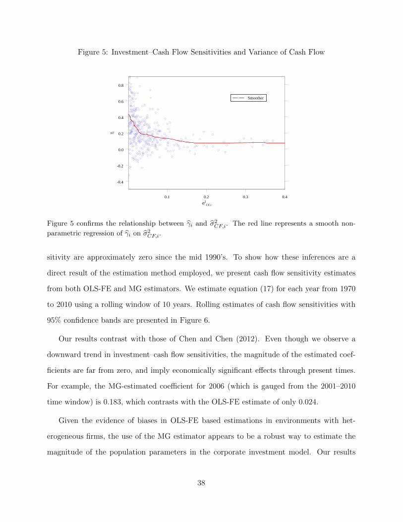
Figure 5: Investment–Cash Flow Sensitivities and Variance of Cash Flow

0.1 0.2 0.3 0.4

σ2CF,i

-0.4

-0.2

0.0

0.2

0.4

0.6

0.8

γ i

Smoother

Figure 5 confirms the relationship between γi and σ2CF,i. The red line represents a smooth non-

parametric regression of γi on σ2CF,i.

sitivity are approximately zero since the mid 1990’s. To show how these inferences are a

direct result of the estimation method employed, we present cash flow sensitivity estimates

from both OLS-FE and MG estimators. We estimate equation (17) for each year from 1970

to 2010 using a rolling window of 10 years. Rolling estimates of cash flow sensitivities with

95% confidence bands are presented in Figure 6.

Our results contrast with those of Chen and Chen (2012). Even though we observe a

downward trend in investment–cash flow sensitivities, the magnitude of the estimated coef-

ficients are far from zero, and imply economically significant effects through present times.

For example, the MG-estimated coefficient for 2006 (which is gauged from the 2001–2010

time window) is 0.183, which contrasts with the OLS-FE estimate of only 0.024.

Given the evidence of biases in OLS-FE based estimations in environments with het-

erogeneous firms, the use of the MG estimator appears to be a robust way to estimate the

magnitude of the population parameters in the corporate investment model. Our results

38

Figure 6: Investment Cash Flow Sensitivity Coefficients

1975 1980 1985 1990 1995 2000 2005Year

-0.1

0.0

0.1

0.2

0.3

0.4

0.5

0.6

Est

imat

ed c

oeff

icie

nts

OLS-FEMGCash Flow Std/10

Figure 6 shows the estimated coefficients of γ using OLS-FE and MG estimation using a rollingwindow of T = 10 time-series observations for each year. The standard deviation of cash flowdivided by 10 is shown for the same rolling window periods.

show that the sensitivity of investment to cash flow remains — in a statistical sense — a

potentially important factor in understanding investment behavior.

6 Conclusion

We show that heterogeneity in individual responses to economic stimuli can distort estimates

that are commonly reported. The theorems and Monte Carlo evidence advanced in this pa-

per show that standard fixed effects models may often render biased estimates of individual

responses in light of slope heterogeneity. Critically, the bias of the fixed effects estimator

can be very pronounced and lead to mistaken economic conclusions.

As part of the exploration of the potential bias in fixed effects estimation, we propose

and analyze new statistical tests that are designed to indicate whether fixed effects is the

appropriate estimator. One interpretation of the proposed tests is that they are testing the

39

moment conditions required for fixed effects estimator to be consistent for corresponding

population parameters of interest. The tests are simple to calculate, governed by a simple

distribution, and shown to be effective in an extensive Monte Carlo experiment. The tests

are intuitive, in that it directly estimates the bias associated with the fixed effects estimator,

and standardizes the estimated bias. The structure of our heterogeneity bias (HB and

HBC) tests are similar to a Wald test, and have chi-square limiting distributions under the

null hypothesis of no heterogeneity bias in the fixed effects estimator. The HBC test is a

generalization of the HB test by allowing for cross-section dependence in the errors and a

form of endogeneity.

Finally, it is worth noting that even if one fails to reject the null hypothesis of no het-

erogeneity bias in fixed effects estimation, the fixed effects estimator may not be efficient.

The results from our Monte Carlo experiment illustrate this fact (when we know that there

is no bias by construction, yet mean group estimators (MG and MGC) have smaller MSE).

Moreover, in our empirical example, we reject the null of no heterogeneity bias for the fixed

effects estimator, yet the standard errors are sometimes smaller or larger for the fixed effects

estimated coefficients. Our results suggest that the Mean Group Correlated estimator of

Pesaran (2006) provides a useful robustness check. The test we propose is a formal way to

check if the mean group estimators (MG and MGC) are the appropriate tool for a given

empirical study.

40

A Appendix

Recall the following definitions: yi = (yi1, ..., yiT )>, Xi = (xi1, ..., xiT )>, ui = (ui1, ..., uiT )>,

Mι = IT − ιT (ι>T ιT )−1ι>T , IT is an identity matrix of order T , ιT is a T × 1 vector of ones.

Proof of Theorem 1: First,

βi − βMG = βi + (X>i MιXi)−1X>i Mιui −

1

N

N∑j=1

(X>j MιXj)−1X>j Mιyj

= βi − β + (X>i MιXi)−1X>i Mιui −

1

N

N∑i=1

(βi − β)− 1

N

N∑j=1

(X>j MιXj)−1X>j Mιuj.

Then,

√Nδ =

1√N

N∑i=1

1

TX>i MιXi

(βi − βMG

)=

1√N

N∑i=1

1

TX>i MιXi(βi − β) +

1√N

N∑i=1

1

T − 1X>i Mιui −

1√N

N∑i=1

1

TX>i MιXi

[1

N

N∑i=1

(βi − β)

]

− 1√N

N∑i=1

1

TX>i MιXi

1

N

N∑j=1

(X>j MιXj)−1X>j Mιuj

=

1√N

N∑i=1

1

TX>i MιXi −

1

N

N∑j=1

1

TX>j MιXj

(βi − β)

+1√N

N∑i=1

1

TX>i Mιui −

1√N

N∑i=1

1

TX>i MιXi

1

N

N∑j=1

(X>j MιXj)−1X>j Mιuj

= A1 +A2.

Let ri = (X>i MιXi)−1X>i Mιui, so that

A2 =1√N

N∑i=1

1

TX>i MιXi(ri − r).

By Assumption 1 and under the null hypothesis, the central limit theorem applies to both

41

terms. Write the terms

A1 =1√N

N∑i=1

A1i,

A2 =1√N

N∑i=1

A2i.

The estimated variance matrix is

Ω =1

N

N∑i=1

1

TX>i MιXi

(βi − βMG

)(βi − βMG

)> 1

TX>i MιXi

=1

N

N∑i=1

(A1iA>1i + A1iA

>2i + A2iA

>1i + A2iA

>2i).

Since A1i and A2i are uncorrelated,

1

N

N∑i=1

A1iA>2i

p→ 0.

Hence, the estimated variance converges to

1

N

N∑i=1

[E(A1iA

>1i) + E(A2iA

>2i)].

The dominant term of the first block contains T−2E[(X>i MιXi)(βi−β)(βi−β)>(X>i MιXi)].

The rank of this term vary from 0 to k. The second block has leading term

1

NT 2

N∑i=1

E[(X>i MιXi)

−1X>i MιΩiMιXi(X>i MιXi)

−1] ,which is full rank, with

Ωi = E(uiu>i |Xi).

42

B Appendix

Proof of Theorem 2: We find the distribution of the normalized estimate of the population

moment condition in question. First,

δC =1√N

N∑i=1

(X>i MQXi

T

)(βCi − βMGC

)=

1√N

N∑i=1

(X>i MQXi

T

)[(βCi − βi) + (βi − β) + (β − βMGC)

]= B1 +B2 +B3.

The first term, B1, can be simplified as

1√N

N∑i=1

(X>i MQXi

T

)(βCi − βi) =

1√N

N∑i=1

(X>i MQXi

T

)(X>i MQXi)

−1X>i MQui

=1√N

N∑i=1

(X>i MQui

T

).

Given Assumptions 4,5,7, and 10, Lemma 2 of Pesaran (2006) still holds, and we have

MQ = MG+Op(N−1)+Op(N

−1/2T−1/2). Hence, we eliminate the factors in ui by the matrix

MG so that

1√N

N∑i=1

(X>i MQui

T

)=

1√N

N∑i=1

(X>i MGεi

T

)+Op(N

−1/2) +Op(T−1/2).

Given the independence across i, we have

E

[1√N

N∑i=1

(X>i MGεi

T

)]2=

1

N

N∑i=1

E

(X>i MGεi

T

)2

= O(T−1),

so that B1 = Op(N−1/2) +Op(T

−1/2).

43

Considering B3, we have

βMGC =1

N

N∑i=1

βCi

=1

N

N∑i=1

[βi + (X>i MQXi)

−1X>i MQui]

= β +1

N

N∑i=1

(βi − β) +1

N

N∑i=1

(X>i MQXi)−1X>i MQui

= β +1

N

N∑i=1

(βi − β) +1

N

N∑i=1

(X>i MGXi)−1X>i MGεi +Op(N

−1) +Op(N−1/2T−1/2).

Noting that

1

N

N∑i=1

(X>i MGXi)−1X>i MGεi = Op(N

−1/2T−1/2),

we have

B3 = −

[1√N

N∑i=1

(X>i MGXi

T

)1

N

N∑i=1

(βi − β)

]+Op(N

−1/2) +Op(T−1/2).

Now combining B2 and B3 we have that

B2 +B3 =1√N

N∑i=1

(X>i MGXi

T

)[(βi − β)− 1

N

N∑j=1

(βj − β)

]+Op(N

−1/2) +Op(T−1/2).

Given Assumption 9, we apply the central limit theorem. The variance of the leading term

is

E

[(X>i MGXi

T

)(βi − β)(βi − β)>

(X>i MGXi

T

)].

44

As in Theorem 1, we can estimate this via

ΩC =1

N − 1

N∑i=1

δCiδ>Ci

=1

N − 1

N∑i=1

(X>i MQXi

T

)(βCi − βMGC

)(βCi − βMGC

)>(X>i MQXi

T

).

This estimator is the analogue of (67) of Pesaran (2006), and consistent for the population

variance.

45

References

Almeida, H., and M. Campello (2007): “Financial Constraints, Asset Tangibility and

Corporate Investment,” Review of Financial Studies, 20, 1429–1460.

Bai, J. (2009): “Panel Data Models with Interactive Fixed Effects,” Econometrica, 77,

1229–1279.

Baker, M., J. C. Stein, and J. Wurgler (2003): “When Does the Market Matter?

Stock Prices and the Investment of Equity-Dependent Firms,” Quarterly Journal of Eco-

nomics, 118, 969–1005.

Blomquist, J., and J. Westerlund (2013): “Testing Slope Homogeneity in Large Panels

with Serial Correlation,” Economics Letters, 121, 374–378.

Breusch, T., and A. Pagan (1979): “A Simple Test for Heteroskedasticity and Random

Coefficient Variation,” Econometrica, 47, 1287–1294.

Chen, H., and S. Chen (2012): “Investment-Cash Flow Sensitivity Cannot be a Good

Measure of Financial Constraints: Evidence from the Time Series,” Journal of Financial

Economics, 103, 390–410.

Cummins, J. G., K. A. Hassett, and S. D. Oliner (2006): “Investment Behavior,

Observable Expectations, and Internal Funds,” American Economic Review, 96, 796–810.

Fazzari, S., R. G. Hubbard, and B. Petersen (1988): “Financing Constraints and

Corporate Investment,” Brooking Papers on Economic Activity, 1, 141–195.

Friedman, J. H. (1984): “A Variable Span Scatterplot Smoother,” Laboratory for Com-

putational Statistics, Stanford University Technical Report No. 5.

Hausman, J. (1978): “Specification tests in econometrics,” Econometrica, 46, 1251–1271.

Hsiao, C. (2003): Analysis of Panel Data. Cambridge University Press, New York, New

York.

Hsiao, C., and M. H. Pesaran (2008): “Random Coefficient Models,” in Advanced

Studies in Theoretical and Applied Econometrics, Vol. 46, The Econometrics of Panel

Data: Fundamentals and Recent Developments in Theory and Practice, ed. by L. Matyas,

and P. Sevestre. Springer-Verlag, Berlin.

Kaplan, S., and L. Zingales (1997): “Do Financing Constraints Explain Why Investment

Is Correlated with Cash Flow?,” Quarterly Journal of Economics, 112, 169–215.

46

Newey, W. K., and D. L. McFadden (1994): “Large Sample Estimation and Hypothesis

Testing,” in Handbook of Econometrics, Vol. 4, ed. by R. F. Engle, and D. L. McFadden.

North Holland, Elsevier, Amsterdam.

Pesaran, H., R. Smith, and K. S. Im (1996): “Dynamic Linear Models for Heterogeneous

Panels,” in The Econometrics of Panel Data: A Handbook of the Theory with Applications,

ed. by L. Matyas, and P. Sevestre, pp. 145–195. Kluwer Academic Publishers, Dordrecht.

Pesaran, M. H. (2006): “Estimation and Inference in Large Heterogeneous Panels with a

Multifactor Error Structure,” Econometrica, 74, 967–1012.

Pesaran, M. H., and R. Smith (1995): “Estimating Long-Run Relationships from Dy-

namic Heterogeneous Panels,” Journal of Econometrics, 68, 79–113.

Pesaran, M. H., and T. Yamagata (2008): “Testing Slope Homogeneity in Large Pan-

els,” Journal of Econometrics, 142, 50–93.

Phillips, P., and D. Sul (2003): “Dynamic Panel Estimation and Homogeneity Testing

under Cross Section Dependence,” Econometrics Journal, 6, 217–259.

Polk, C., and P. Sapienza (2009): “The Stock Market and Corporate Investment: A

Test of Catering Theory,” Review of Financial Studies, 22, 187–217.

Rauh, J. (2006): “Investment and Financing Constraints: Evidence from the Funding of

Corporate Pension Plans,” Journal of Finance, 61, 33–71.

Schaller, H. (1990): “A Re-Examination of the Q Theory of Investment Using U.S. Firm

Data,” Journal of Applied Econometrics, 5, 309–325.

Su, L., and Q. Chen (2013): “Testing Homogeneity in Panel Data Models with Interactive

Fixed Effects,” Econometric Theory, 29, 1079–1135.

Swamy, P. A. V. B. (1970): “Efficient Inference in a Random Coefficient Regression

Model,” Econometrica, 38, 311–323.

Wooldridge, J. M. (2003): “Fixed Effects Estimation of the Population-Averaged Slopes

in a Panel Data Random Coefficient Model,” Econometric Theory, 19, 411–413.

(2005): “Fixed-Effects and Related Estimators for Correlated Random-Coefficient

and Treatment-Effect Panel Data Models,” Review of Economics and Statistics, 87, 385–

390.

(2010): Econometric Analysis of Cross Section and Panel Data, 2nd Edition. The

MIT Press, Cambridge, Maryland.

47

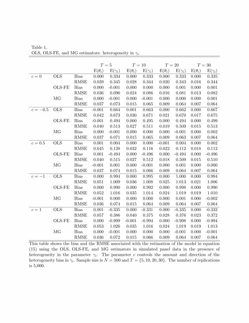
Table 1.OLS, OLS-FE, and MG estimators: heterogeneity in γi

T = 5 T = 10 T = 20 T = 30E(θi) E(γi) E(θi) E(γi) E(θi) E(γi) E(θi) E(γi)

c = 0 OLS Bias 0.000 0.334 0.000 0.333 0.000 0.333 0.000 0.335RMSE 0.039 0.345 0.028 0.344 0.020 0.343 0.016 0.344

OLS-FE Bias 0.000 -0.001 0.000 0.000 0.000 0.001 0.000 0.001RMSE 0.036 0.096 0.024 0.086 0.016 0.081 0.013 0.082

MG Bias 0.000 -0.001 0.000 -0.001 0.000 0.000 0.000 0.001RMSE 0.037 0.073 0.015 0.065 0.009 0.064 0.007 0.064

c = −0.5 OLS Bias -0.001 0.664 0.001 0.663 0.000 0.662 0.000 0.667RMSE 0.042 0.673 0.030 0.671 0.021 0.670 0.017 0.675

OLS-FE Bias -0.001 0.494 0.000 0.495 0.000 0.494 0.000 0.499RMSE 0.040 0.513 0.027 0.511 0.019 0.509 0.015 0.513

MG Bias 0.000 -0.001 0.000 0.000 0.000 -0.001 0.000 0.002RMSE 0.037 0.071 0.015 0.065 0.009 0.063 0.007 0.064

c = 0.5 OLS Bias 0.001 0.004 0.000 0.000 -0.001 0.004 0.000 0.002RMSE 0.045 0.128 0.032 0.116 0.022 0.112 0.018 0.112

OLS-FE Bias 0.001 -0.494 0.000 -0.496 0.000 -0.494 0.000 -0.496RMSE 0.040 0.515 0.027 0.512 0.018 0.509 0.015 0.510

MG Bias -0.001 0.001 0.000 -0.001 0.000 0.001 0.000 0.000RMSE 0.037 0.074 0.015 0.066 0.009 0.064 0.007 0.064

c = −1 OLS Bias 0.000 0.994 0.000 0.995 0.000 1.000 0.000 0.994RMSE 0.051 1.009 0.036 1.008 0.025 1.013 0.021 1.006

OLS-FE Bias 0.000 0.990 0.000 0.992 0.000 0.998 0.000 0.990RMSE 0.052 1.016 0.035 1.014 0.024 1.019 0.019 1.010

MG Bias -0.001 0.000 0.000 0.000 0.000 0.001 0.000 -0.002RMSE 0.036 0.074 0.015 0.064 0.009 0.064 0.007 0.064

c = 1 OLS Bias 0.001 -0.335 0.000 -0.331 0.000 -0.335 0.000 -0.332RMSE 0.057 0.386 0.040 0.375 0.028 0.376 0.023 0.372

OLS-FE Bias 0.000 -0.999 -0.001 -0.994 0.000 -0.998 0.000 -0.994RMSE 0.053 1.026 0.035 1.016 0.024 1.019 0.019 1.013

MG Bias 0.000 -0.001 0.000 0.000 0.000 -0.001 0.000 -0.001RMSE 0.036 0.072 0.015 0.066 0.009 0.064 0.007 0.064

This table shows the bias and the RMSE associated with the estimation of the model in equation(15) using the OLS, OLS-FE, and MG estimators in simulated panel data in the presence ofheterogeneity in the parameter γi. The parameter c controls the amount and direction of theheterogeneity bias in γi. Sample size is N = 500 and T = 5, 10, 20, 30. The number of replicationsis 5,000.

Table 2.OLS, OLS-FE, and MG estimators: heterogeneity in θi and γi

T = 5 T = 10 T = 20 T = 30E(θi) E(γi) E(θi) E(γi) E(θi) E(γi) E(θi) E(γi)

c = 0 OLS Bias 0.002 0.331 -0.001 0.333 0.002 0.331 -0.001 0.334RMSE 0.102 0.345 0.090 0.344 0.086 0.341 0.083 0.344

OLS-FE Bias 0.002 -0.003 -0.001 0.001 0.001 0.000 -0.001 0.001RMSE 0.103 0.102 0.088 0.088 0.084 0.082 0.082 0.080

MG Bias 0.000 -0.001 0.000 0.000 0.001 0.001 0.000 0.000RMSE 0.075 0.074 0.064 0.065 0.064 0.064 0.064 0.064

c = −0.5 OLS Bias 0.497 0.664 0.497 0.664 0.497 0.666 0.498 0.665RMSE 0.519 0.675 0.514 0.673 0.513 0.674 0.513 0.672

OLS-FE Bias 0.497 0.495 0.498 0.497 0.497 0.499 0.498 0.497RMSE 0.519 0.517 0.514 0.514 0.512 0.514 0.513 0.511

MG Bias 0.000 -0.001 -0.001 0.000 0.001 0.001 0.000 0.001RMSE 0.072 0.073 0.064 0.064 0.064 0.064 0.064 0.063

c = 0.5 OLS Bias -0.497 0.003 -0.495 0.001 -0.497 0.002 -0.499 0.000RMSE 0.519 0.129 0.513 0.121 0.513 0.118 0.513 0.114

OLS-FE Bias -0.497 -0.495 -0.495 -0.497 -0.497 -0.495 -0.499 -0.498RMSE 0.519 0.516 0.512 0.514 0.512 0.511 0.514 0.512

MG Bias -0.001 0.001 0.001 0.000 0.000 0.000 -0.001 0.000RMSE 0.073 0.072 0.065 0.065 0.064 0.064 0.065 0.064

c = −1 OLS Bias 0.990 0.995 0.996 0.994 0.997 0.998 0.994 0.998RMSE 1.018 1.011 1.018 1.007 1.018 1.010 1.014 1.010

OLS-FE Bias 0.990 0.991 0.995 0.988 0.997 0.994 0.994 0.995RMSE 1.018 1.020 1.018 1.011 1.017 1.015 1.014 1.014

MG Bias -0.002 0.000 0.001 0.000 0.001 0.000 -0.001 0.000RMSE 0.073 0.073 0.065 0.064 0.064 0.062 0.063 0.065

c = 1 OLS Bias -0.991 -0.328 -0.993 -0.331 -0.992 -0.332 -0.998 -0.329RMSE 1.018 0.381 1.015 0.376 1.013 0.375 1.019 0.369

OLS-FE Bias -0.991 -0.988 -0.995 -0.991 -0.992 -0.997 -0.998 -0.991RMSE 1.019 1.017 1.016 1.014 1.012 1.017 1.019 1.010

MG Bias 0.001 0.000 0.001 0.000 0.001 -0.001 -0.001 0.000RMSE 0.074 0.073 0.065 0.065 0.064 0.065 0.065 0.062

This table shows the bias and the RMSE associated with the estimation of the model in equation(15) using the OLS, OLS-FE, and MG estimators in simulated panel data in the presence ofheterogeneity in the parameters θi and γi. The parameter c controls the amount and direction ofthe heterogeneity bias in both θi and γi. Sample size is N = 500 and T = 5, 10, 20, 30. Thenumber of replications is 5,000.

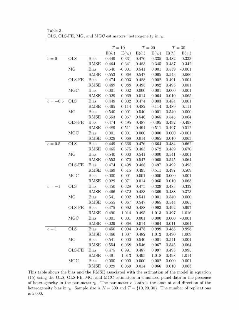
Table 3.OLS, OLS-FE, MG, and MGC estimators: heterogeneity in γi

T = 10 T = 20 T = 30E(θi) E(γi) E(θi) E(γi) E(θi) E(γi)

c = 0 OLS Bias 0.449 0.331 0.476 0.335 0.482 0.333RMSE 0.464 0.341 0.483 0.345 0.487 0.342

MG Bias 0.540 -0.001 0.541 0.001 0.539 -0.001RMSE 0.553 0.068 0.547 0.065 0.543 0.066

OLS-FE Bias 0.474 -0.003 0.488 0.002 0.491 -0.001RMSE 0.489 0.088 0.495 0.082 0.495 0.081

MGC Bias 0.001 -0.002 0.000 0.001 0.000 -0.001RMSE 0.029 0.069 0.014 0.064 0.010 0.065

c = −0.5 OLS Bias 0.449 0.002 0.474 0.003 0.484 0.001RMSE 0.465 0.114 0.482 0.114 0.489 0.111

MG Bias 0.540 0.001 0.540 0.001 0.540 0.000RMSE 0.553 0.067 0.546 0.065 0.545 0.064

OLS-FE Bias 0.474 -0.495 0.487 -0.495 0.492 -0.498RMSE 0.489 0.511 0.494 0.511 0.497 0.512

MGC Bias 0.001 0.001 0.000 0.000 0.000 -0.001RMSE 0.029 0.068 0.014 0.065 0.010 0.063

c = 0.5 OLS Bias 0.449 0.666 0.476 0.664 0.484 0.662RMSE 0.465 0.675 0.483 0.672 0.489 0.670

MG Bias 0.540 0.000 0.541 0.000 0.541 -0.001RMSE 0.553 0.070 0.547 0.065 0.545 0.064

OLS-FE Bias 0.474 0.498 0.488 0.497 0.492 0.495RMSE 0.489 0.515 0.495 0.511 0.497 0.509

MGC Bias 0.000 0.001 0.001 0.000 0.000 -0.001RMSE 0.029 0.071 0.014 0.065 0.010 0.063

c = −1 OLS Bias 0.450 -0.328 0.475 -0.329 0.483 -0.332RMSE 0.466 0.372 0.483 0.369 0.488 0.373

MG Bias 0.541 0.002 0.541 0.001 0.540 0.000RMSE 0.555 0.067 0.547 0.065 0.544 0.065

OLS-FE Bias 0.475 -0.992 0.488 -0.993 0.492 -0.997RMSE 0.490 1.014 0.495 1.013 0.497 1.016

MGC Bias 0.001 0.001 0.001 0.000 0.000 -0.001RMSE 0.029 0.068 0.014 0.064 0.011 0.064

c = 1 OLS Bias 0.450 0.994 0.475 0.999 0.485 0.998RMSE 0.466 1.007 0.482 1.012 0.490 1.009

MG Bias 0.541 0.000 0.540 0.001 0.541 0.001RMSE 0.554 0.068 0.546 0.067 0.545 0.064

OLS-FE Bias 0.475 0.991 0.487 0.997 0.493 0.995RMSE 0.491 1.013 0.495 1.018 0.498 1.014

MGC Bias 0.000 0.000 0.000 0.002 0.000 0.001RMSE 0.029 0.069 0.014 0.066 0.010 0.063

This table shows the bias and the RMSE associated with the estimation of the model in equation(15) using the OLS, OLS-FE, MG, and MGC estimators in simulated panel data in the presenceof heterogeneity in the parameter γi. The parameter c controls the amount and direction of theheterogeneity bias in γi. Sample size is N = 500 and T = 10, 20, 30. The number of replicationsis 5,000.

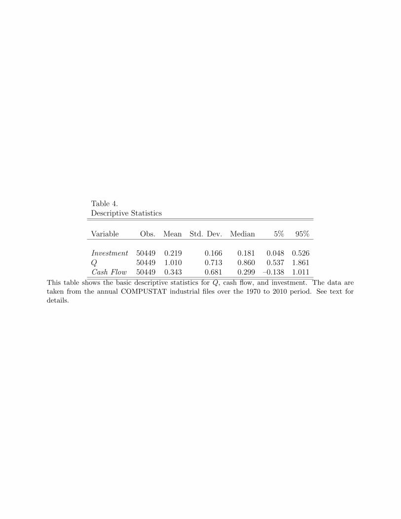
Table 4.Descriptive Statistics

Variable Obs. Mean Std. Dev. Median 5% 95%

Investment 50449 0.219 0.166 0.181 0.048 0.526Q 50449 1.010 0.713 0.860 0.537 1.861Cash Flow 50449 0.343 0.681 0.299 –0.138 1.011

This table shows the basic descriptive statistics for Q, cash flow, and investment. The data aretaken from the annual COMPUSTAT industrial files over the 1970 to 2010 period. See text fordetails.

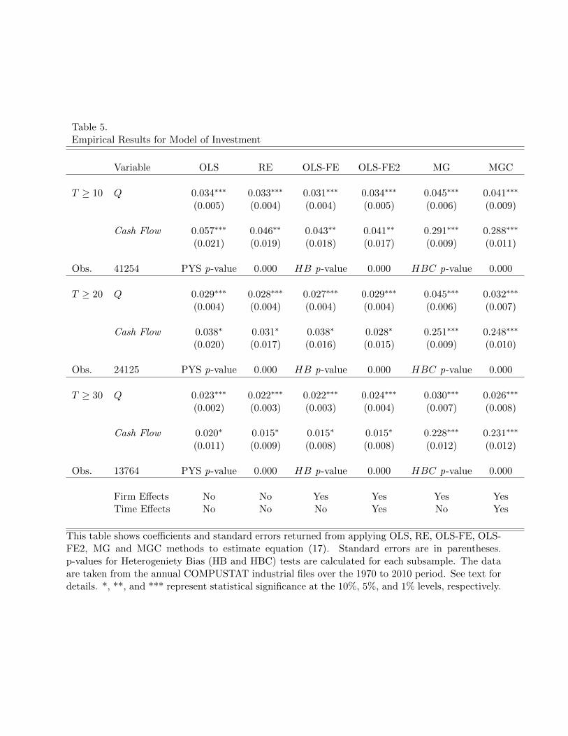
Table 5.Empirical Results for Model of Investment

Variable OLS RE OLS-FE OLS-FE2 MG MGC

T ≥ 10 Q 0.034∗∗∗ 0.033∗∗∗ 0.031∗∗∗ 0.034∗∗∗ 0.045∗∗∗ 0.041∗∗∗

(0.005) (0.004) (0.004) (0.005) (0.006) (0.009)

Cash Flow 0.057∗∗∗ 0.046∗∗ 0.043∗∗ 0.041∗∗ 0.291∗∗∗ 0.288∗∗∗

(0.021) (0.019) (0.018) (0.017) (0.009) (0.011)

Obs. 41254 PYS p-value 0.000 HB p-value 0.000 HBC p-value 0.000

T ≥ 20 Q 0.029∗∗∗ 0.028∗∗∗ 0.027∗∗∗ 0.029∗∗∗ 0.045∗∗∗ 0.032∗∗∗

(0.004) (0.004) (0.004) (0.004) (0.006) (0.007)

Cash Flow 0.038∗ 0.031∗ 0.038∗ 0.028∗ 0.251∗∗∗ 0.248∗∗∗

(0.020) (0.017) (0.016) (0.015) (0.009) (0.010)

Obs. 24125 PYS p-value 0.000 HB p-value 0.000 HBC p-value 0.000

T ≥ 30 Q 0.023∗∗∗ 0.022∗∗∗ 0.022∗∗∗ 0.024∗∗∗ 0.030∗∗∗ 0.026∗∗∗

(0.002) (0.003) (0.003) (0.004) (0.007) (0.008)

Cash Flow 0.020∗ 0.015∗ 0.015∗ 0.015∗ 0.228∗∗∗ 0.231∗∗∗

(0.011) (0.009) (0.008) (0.008) (0.012) (0.012)

Obs. 13764 PYS p-value 0.000 HB p-value 0.000 HBC p-value 0.000

Firm Effects No No Yes Yes Yes YesTime Effects No No No Yes No Yes

This table shows coefficients and standard errors returned from applying OLS, RE, OLS-FE, OLS-FE2, MG and MGC methods to estimate equation (17). Standard errors are in parentheses.p-values for Heterogeniety Bias (HB and HBC) tests are calculated for each subsample. The dataare taken from the annual COMPUSTAT industrial files over the 1970 to 2010 period. See text fordetails. *, **, and *** represent statistical significance at the 10%, 5%, and 1% levels, respectively.