Static Panel Data Models1

Class Notes

Manuel Arellano

Revised: October 9, 2009

1 Unobserved Heterogeneity

The econometric interest in panel data has been the result of two different motivations:

• First, the desire of exploiting panel data for controlling unobserved time-invariant heterogeneityin cross-sectional models.

• Second, the use of panel data to disentangle components of variance and estimating transitionprobabilities, and more generally to study the dynamics of cross-sectional populations.

These motivations can be loosely associated with two strands of the panel data literature labelled

fixed effects and random effects models. We next take these two motivations and models in turn.

1.1 Overview

A sizeable part of econometric activity deals with empirical description and forecasting, but another

aims at quantifying structural or causal relationships. Structural relations are needed for policy

evaluation and for testing theories.

The regression model is an essential tool for descriptive and structural econometrics. However,

regression lines from economic data often cannot be given a causal interpretation. The reason is that

sometimes we expect correlation between explanatory variables and errors in the relation of interest.

One example is the classical supply-and-demand simultaneity problem due market equilibrium.

Another is measurement error: if the explanatory variable we observe is not the variable to whom

agents respond but an error ridden measure of it, the unobservable term in the equation of interest

will contain the measurement error, which will be correlated with the regressor. Finally, there may

be correlation due to unobserved heterogeneity. This has been a pervasive problem in cross-sectional

regression analysis. If characteristics that have a direct effect on both left- and right-hand side variables

are omitted, explanatory variables will be correlated with errors and regression coefficients will be

biased measures of the structural effects. Thus, researchers have often been confronted with massive

cross-sectional data sets from which precise correlations can be determined but that, nevertheless, had

no information about parameters of policy interest.

1This is an abridged version of Part I in Arellano (2003).

1

The traditional response of econometrics to these problems has been multiple regression and in-

strumental variable models. Regrettably, we often lack data on the conditioning variables or the

instruments to achieve identification of structural parameters in these ways.

A major motivation for using panel data has been the ability to control for possibly correlated,

time-invariant heterogeneity without observing it. Suppose a cross-sectional regression of the form

yi1 = βxi1 + ηi + vi1 (1)

such that E(vi1 | xi1, ηi) = 0. If ηi is observed β can be identified from a multiple regression of y on x

and η. If ηi is not observed identification of β requires either lack of correlation between xi1 and ηi,

in which case

Cov(xi1,ηi) = 0⇒ β =Cov(xi1, yi1)

V ar(xi1),

or the availability of an external instrument zi that is uncorrelated with both vi1 and ηi but correlated

with xi1, in which case

Cov(zi,ηi) = 0⇒ β =Cov(zi, yi1)

Cov(zi, xi1).

Suppose that neither of these two options is available, but we observe yi2 and xi2 for the same

individuals in a second period (so that T = 2) such that

yi2 = βxi2 + ηi + vi2 (2)

and both vi1 and vi2 satisfy E(vit | xi1, xi2, ηi) = 0. Then β is identified in the regression in first-

differences even if ηi is not observed. We have:

yi2 − yi1 = β(xi2 − xi1) + (vi2 − vi1) (3)

and

β =Cov(∆xi2,∆yi2)

V ar(∆xi2). (4)

AClassic Example:Agricultural Production (Mundlak 1961, Chamberlain 1984) Sup-

pose equation (1) represents the Cobb-Douglas production function of an agricultural product. The

index i denotes farms and t time periods (seasons or years). Also:

yit = Log output.

xit = Log of a variable input (labour).

ηi = An input that remains constant over time (soil quality).

vit = A stochastic input which is outside the farmer’s control (rainfall).

2

Suppose ηi is known by the farmer but not by the econometrician. If farmers maximize expected

profits there will be cross-sectional correlation between labour and soil quality. Therefore, the pop-

ulation coefficient in a simple regression of yi1 on xi1 will differ from β. If η were observed by the

econometrician, the coefficient on x in a multiple cross-sectional regression of yi1 on xi1 and ηi will

coincide with β. Now suppose that data on yi2 and xi2 for a second period become available. Moreover,

suppose that rainfall in the second period is unpredictable from rainfall in the first period (permanent

differences in rainfall are part of ηi), so that rainfall is independent of a farm’s labour demand in

the two periods. Thus, even in the absence of data on ηi the availability of panel data affords the

identification of the technological parameter β.

A Firm Money Demand Example (Bover and Watson, 2005) Suppose firms minimize

cost for given output sit subject to a production function sit = F (xit) and to some transaction services

sit =³aim

(1−b)it

bit

´1/c, where x denotes a composite input, m is demand for cash, is labour employed

in transactions, and a represents the firm’s financial sophistication. There will be economies of scale

in the demand for money by firms if c 6= 1. The resulting money demand equation is

logmit = k + c log sit − b log(Rit/wit)− log ai + vit. (5)

Here k is a constant, R is the opportunity cost of holding money, w is the wage of workers involved

in transaction services, and v is a measurement error in the demand for cash. In general a will be

correlated with output through the cash-in-advance constraint. Thus, the coefficient of output (or

sales) in a regression of logm on log s and log(R/w) will not coincide with the scale parameter of

interest. However, if firm panel data is available and a varies across firms but not over time in the

period of analysis, economies of scale can be identified from the regression in changes.

An Example in which Panel Data Does Not Work: Returns to Education “Structural”

returns to education are important in the assessment of educational policies. It has been widely

believed in the literature that cross-sectional regression estimates of the returns could not be trusted

because of omitted “ability” potentially correlated with education attainment. In the earlier notation:

yit = Log wage (or earnings).

xit = Years of full-time education.

ηi = Unobserved ability.

β = Returns to education.

The problem in this example is that xit typically lacks time variation. So a regression in first-

differences will not be able to identify β in this case. In this context data on siblings and cross-sectional

instrumental variables have proved more useful for identifying returns to schooling free of ability bias

than panel data (Griliches, 1977).

3

This example illustrates a more general problem. Information about β in the regression in first-

differences will depend on the ratio of the variances of∆v and∆x. In the earnings−education equation,we are in the extreme situation where V ar(∆x) = 0, but if V ar(∆x) is small regressions in changes

may contain very little information about parameters of interest even if the cross-sectional sample size

is very large.

Econometric Measurement versus Forecasting Problems The previous examples suggest

that the ability to control for unobserved heterogeneity is mainly an advantage in the context of

problems of econometric measurement as opposed to problems of forecasting. This is an important

distinction. Including individual effects we manage to identify certain coefficients at the expense of

leaving part of the regression unmodelled (the one that only has cross-sectional variation).

The part of the variance of y accounted by xβ could be very small relative to η and v. In a case

like this it would be easy to obtain higher R2 by including lagged dependent variables or proxies for

the fixed effects. Regressions of this type would be useful in cross-sectional forecasting exercises for

the population from which the data come (like in credit scoring or in the estimation of probabilities

of tax fraud), but they may be of no use if the objective is to measure the effect of x on y holding

constant all time-invariant heterogeneity.

An equation with individual specific intercepts may still be useful when the interest is in forecasts

for the same individuals in different time periods, but not when we are interested in forecasts for

individuals other than those included in the sample.

Non-Exogeneity andRandomCoefficients The identification of causal effects through regres-

sion coefficients in differences or deviations depends on the lack of correlation between x and v at

all lags and leads (strict exogeneity). If x is measured with error or is correlated with lagged errors,

regressions in deviations may actually make things worse.

Another difficulty arises when the effect of x on y is itself heterogeneous. In such case regres-

sion coefficients in differences cannot in general be interpreted as average causal effects. Specifically,

suppose that β is allowed to vary cross-sectionally in (1) and (2) so that

yit = βixit + ηi + vit (t = 1, 2) E (vit | xi1, xi2, ηi,βi) = 0. (6)

In these circumstances, the regression coefficient (4) differs from E (βi) unless βi is mean independent

of ∆xi2. The availability of panel data still affords identification of average causal effects in random

coefficients models as long as x is strictly exogenous. However, if x is not exogenous and βi is

heterogeneous we run into serious identification problems in short panels.

4

1.2 Fixed Effects Models

1.2.1 Assumptions

Our basic assumptions for what we call the “static fixed effects model” are as follows. We assume that

(yi1, ..., yiT , xi1, ..., xiT , ηi), i = 1, ...,N is a random sample and that

yit = x0itβ + ηi + vit (7)

together with

Assumption A1:

E(vi | xi, ηi) = 0 (t = 1, ..., T ),

where vi = (vi1, ..., viT )0 and xi = (x0i1, ..., x0iT )

0. We observe yit and the k × 1 vector of explanatoryvariables xit but not ηi, which is therefore an unobservable time-invariant regressor.

Similarly, we shall refer to “classical” errors when the additional auxiliary assumption holds:

Assumption A2:

V ar(vi | xi, ηi) = σ2IT .

Under Assumption A2 the errors are conditionally homoskedastic and not serially correlated.

Under Assumption A1 we have

E(yi | xi, ηi) = Xiβ + ηiι (8)

where yi = (yi1, ..., yiT )0, ι is a T × 1 vector of ones, and Xi = (xi1, ..., xiT )0 is a T × k matrix. Theimplication of (8) for the expected value of yi given xi is

E(yi | xi) = Xiβ +E(ηi | xi)ι. (9)

Moreover, under Assumption A2

V ar(yi | xi, ηi) = σ2IT , (10)

which implies

V ar(yi | xi) = σ2IT + V ar(ηi | xi)ιι0. (11)

A1 is the fundamental assumption in this context. It implies that the error v at any period

is uncorrelated with past, present, and future values of x (or, conversely, that x at any period is

uncorrelated with past, present, and future values of v). A1 is, therefore, an assumption of strict

exogeneity that rules out, for example, the possibility that current values of x are influenced by

5

past errors. In the agricultural production function example, x (labour) will be uncorrelated with v

(rainfall) at all lags and leads provided the latter is unpredictable from past rainfall (given permanent

differences in rainfall that would be subsumed in the farm effects, and possibly seasonal or other

deterministic components). If rainfall in period t is predictable from rainfall in period t−1–which isknown to the farmer in t–labour demand in period t will in general depend on vi(t−1) (Chamberlain,

1984, 1258—1259).

Assumption A2 is, on the other hand, an auxiliary assumption under which classical least-squares

results are optimal. However, lack of compliance with A2 is often to be expected in applications.

Here, we first present results under A2, and subsequently discuss estimation and inference with het-

eroskedastic and serially correlated errors.

As for the nature of the effects, strictly speaking, the term fixed effects would refer to a sampling

process in which the same units are (possibly) repeatedly sampled for a given period holding constant

the effects. In such context one often has in mind a distribution of individual effects chosen by the

researcher. Here we imagine a sample randomly drawn from a multivariate population of observable

data and unobservable effects. This notion may or may not correspond to the physical nature of data

collection. It would be so, for example, in the case of some household surveys, but not with data

on all quoted firms or OECD countries. In those cases, the multivariate population from which the

data come is hypothetical. Moreover, we are interested in models which only specify features of the

conditional distribution f (yi | xi, ηi). Therefore, we are not concerned with whether the distributionthat generates the data on xi and ηi, f (xi, ηi) say, is representative of some cross-sectional population

or of the researcher’s wishes. We just regard (yi, xi, ηi) as a random sample from the (perhaps artificial)

multivariate population with joint distribution f (yi, xi, ηi) = f (yi | xi, ηi) f (xi, ηi) and focus on theconditional distribution of yi. So in common with much of the econometric literature, we use the term

fixed effects to refer to a situation in which f (ηi | xi) is left unrestricted.

1.2.2 Within-Group Estimation

With T = 2 there is just one equation after differencing. Under Assumptions A1 and A2, the equation

in first differences is a classical regression model and hence OLS in first-differences is the optimal

estimator of β in the least squares sense. To see the irrelevance of the equations in levels in this

model, note that a non-singular transformation of the original two-equation system is

E (yi1 | xi) = x0i1β +E (ηi | xi)

E (∆yi2 | xi) = ∆x0i2β.

Since E (ηi | xi) is an unknown unrestricted function of xi, knowledge of the function E (yi1 | xi) isuninformative about β in the first-equation. Thus, no information about β is lost by only considering

the equation in first-differences.

6

If T ≥ 3 we have a system of T − 1 equations in first-differences:∆yi2 = ∆x0i2β +∆vi2

...

∆yiT = ∆x0iTβ +∆viT ,

which in compact form can be written as

Dyi = DXiβ +Dvi, (12)

where D is the (T − 1)× T matrix first-difference operator

D =

⎛⎜⎜⎜⎜⎜⎝−1 1 0 · · · 0 0

0 −1 1 0 0...

. . ....

0 0 0 · · · −1 1

⎞⎟⎟⎟⎟⎟⎠ . (13)

Provided each of the errors in first-differences are mean independent of the xs for all periods (under

Assumption A1 ) E(Dvi | xi) = 0, OLS estimates of β in this system given by

bβOLS =Ã

NXi=1

(DXi)0DXi

!−1 NXi=1

(DXi)0Dyi (14)

will be unbiased and consistent for largeN . However, if the vs are homoskedastic and non-autocorrelated

classical errors (under Assumption A2 ), the errors in first-differences will be correlated for adjacent

periods with

V ar(Dvi | xi) = σ2DD0. (15)

Following standard regression theory, the optimal estimator in this case is given by generalized

least-squares (GLS), which takes the form

bβWG =

ÃNXi=1

X 0iD

0 ¡DD0¢−1DXi!−1 NXi=1

X 0iD

0 ¡DD0¢−1Dyi. (16)

In this case GLS itself is a feasible estimator since DD0 does not depend on unknown coefficients.

The idempotent matrix D0 (DD0)−1D also takes the form2

D0¡DD0

¢−1D = IT − ιι0/T ≡ Q, say. (17)

2To verify this, note that the T × T matrix

H =T−1/2ι0

(DD0)−1/2D

is such that HH0 = IT , so that also H0H = IT or

ιι0/T +D0 DD0 −1D = IT .

7

The matrix Q is known as the within-group operator because it transforms the original time series

into deviations from time means: eyi = Qyi, whose elements are given byeyit = yit − yi

with yi = T−1PT

s=1 yis. Therefore, bβWG can also be expressed as OLS in deviations from time means

bβWG =

"NXi=1

TXt=1

(xit − xi) (xit − xi)0#−1 NX

i=1

TXt=1

(xit − xi) (yit − yi) . (18)

This is probably the most popular estimator in panel data analysis, and it is known under a variety

of names including within-group and covariance estimator.3

It is also known as the dummy-variable least-squares or “fixed effects” estimator. This name

reflects the fact that since bβWG is a least-squares estimator after subtracting individual means to

the observations, it is numerically the same as the estimator of β that would be obtained in a OLS

regression of y on x and a set of N dummy variables, one for each individual in the sample. Thus bβWG

can also be regarded as the result of estimating jointly by OLS β and the realizations of the individual

effects that appear in the sample.

To see this, consider the system of T equations in levels

yi = Xiβ + ιηi + vi

and write it in stacked form as

y = Xβ + Cη + v, (19)

where y=(y01, ..., y0N )0 and v=(v01, ..., v0N )

0 are NT × 1 vectors, X=(X 01, ...,X

0N )

0 is an NT × k matrix,C is an NT ×N matrix of individual dummies given by C = IN ⊗ ι, and η = (η1, ..., ηN)

0 is the N × 1vector of individual specific effects or intercepts. Using the result from partitioned regression, the OLS

regression of y on X and C gives the following expression for estimated β£X 0 ¡INT − C(C 0C)−1C 0¢X¤−1X 0 ¡INT − C(C 0C)−1C 0¢ y, (20)

which clearly coincides with bβWG since INT − C(C 0C)−1C 0 = IN ⊗Q.The expressions for the estimated effects are

bηi = 1

T

TXt=1

³yit − x0itbβWG

´≡ yi − x0ibβWG (i = 1, ..., N). (21)

3The name “within-group” originated in the context of data with a group structure (like data on families and family

members). Panel data can be regarded as a special case of this type of data in which the “group” is formed by the time

series observations from a given individual.

8

We do not need to go beyond standard regression theory to obtain the sampling properties of these

estimators. The fact that bβWG is the GLS for the system of T −1 equations in first-differences tells usthat it will be unbiased and optimal in finite samples. It will also be consistent as N tends to infinity

for fixed T and asymptotically normal under usual regularity conditions. The bηi will also be unbiasedestimates of the ηi for samples of any size, but being time series averages, their variance can only tend

to zero as T tends to infinity. Therefore, they cannot be consistent estimates for fixed T and large

N . Clearly, the within-group estimates bβWG will also be consistent as T tends to infinity regardless

of whether N is fixed or not.

Fixed effects models have a long tradition in econometrics. Their use was first suggested in two

Cowles Commission papers by Clifford Hildreth in 1949 and 1950, and early applications were con-

ducted by Mundlak (1961) and Hoch (1962). The motivation in these two studies was to rely on fixed

effects in order to control for simultaneity bias in the estimation of agricultural production functions.

Orthogonal Deviations Finally, it is worth finding out the form of the transformation to the

original data that results from doing first-differences and further applying a GLS transformation to

the differenced data to remove the moving-average serial correlation induced by differencing (Arellano

and Bover, 1995). The required transformation is given by the (T − 1)× T matrix

A =¡DD0

¢−1/2D.

If we choose (DD0)−1/2 to be the upper triangular Cholesky factorization, the operator A is such that

a T × 1 time series error transformed by A, v∗i = Avi consists of T − 1 elements of the form

v∗it = ct[vit −1

(T − t)(vi(t+1) + ...viT )] (22)

where c2t = (T−t)/(T−t+1). Clearly, A0A = Q and AA0 = IT−1. We then refer to this transformationas forward orthogonal deviations. Thus, if V ar(vi) = σ2IT we also have V ar(v∗i ) = σ2IT−1. So

orthogonal deviations can be regarded as an alternative transformation, which in common with first-

differencing eliminates individual effects but in contrast it does not introduce serial correlation in the

transformed errors. Moreover, the within-group estimator can also be regarded as OLS in orthogonal

deviations.

1.3 Heteroskedasticity and Serial Correlation

1.3.1 Robust Standard Errors for Within-Group Estimators

If assumption A1 holds but A2 does not (that is, using orthogonal deviations, if E(v∗i | xi) = 0 butV ar(v∗i | xi) 6= σ2IT−1), the ordinary regression formulae for estimating the within-group variance will

lead to inconsistent standard errors. Such formula is given by

dV ar(bβWG) = bσ2(X∗0X∗)−1 (23)

9

where X∗ = (IN ⊗A)X, y∗ = (IN ⊗A)y, and bσ2 is the unbiased residual variancebσ2 = 1

N (T − 1)− k (y∗ −X∗bβWG)

0(y∗ −X∗bβWG). (24)

However, sinceµ1

NX∗0X∗

¶√N(bβWG − β) =

1√N

NXi=1

X∗0i v∗i

and E(X∗0i v∗i ) = 0, the right-hand side of the previous expression is a scaled sample average of zero-

mean random variables to which a standard central limit theorem for multivariate iid observations

can be applied for fixed T as N tends to infinity:

1√N

NXi=1

X∗0i v∗id→ N £

0, E(X∗0i v∗i v∗0i X

∗i )¤.

Therefore, an estimate of the asymptotic variance of the within-group estimator that is robust to

heteroskedasticity and serial correlation of arbitrary forms for fixed T and large N can be obtained as

gV ar(bβWG) = (X∗0X∗)−1

ÃNXi=1

X∗0i bv∗i bv∗0i X∗i!(X∗0X∗)−1 (25)

with bv∗i = y∗i −X∗i bβWG (Arellano, 1987). The square root of diagonal elements of gV ar(bβWG) provide

standard errors clustered by individual.

1.3.2 Optimal GLS with Heteroskedasticity and Autocorrelation of Unknown Form

If V ar(v∗i | xi) = Ω(xi) where Ω(xi) is a symmetric matrix of order T−1 containing unknown functionsof xi, the optimal estimator of β will be of the form

bβUGLS =Ã

NXi=1

X∗0i Ω−1(xi)X∗i

!−1 NXi=1

X∗0i Ω−1(xi)y∗i . (26)

This estimator is unfeasible because Ω(xi) is unknown. A feasible semi parametric GLS estimator

would use instead a nonparametric estimator of E(v∗i v∗0i | xi) based on within-group residuals. Under

appropriate regularity conditions and a suitable choice of nonparametric estimator, feasible GLS can

be shown to attain for large N the same efficiency as bβUGLS .A special case which gives rise to a straightforward feasible GLS (for small T and large N), first

discussed by Kiefer (1980), is one in which the conditional variance of v∗i is a constant but non-scalar

matrix: V ar(v∗i | xi) = Ω. This assumption rules out conditional heteroskedasticity, but allows forautocorrelation and unconditional time series heteroskedasticity in the original equation errors vit. In

this case, a feasible GLS estimator takes the form

bβFGLS =Ã

NXi=1

X∗0i bΩ−1X∗i!−1 NX

i=1

X∗0i bΩ−1y∗i (27)

10

where bΩ is given by the orthogonal-deviation WG residual intertemporal covariance matrixbΩ = 1

N

NXi=1

bv∗i bv∗0i . (28)

1.3.3 Improved GMM under Heteroskedasticity and Autocorrelation of Unknown Form

The basic condition E(v∗i | xi) = 0 implies that any function of xi is uncorrelated to v∗i and thereforea potential instrumental variable. Thus, any list of moment conditions of the form

E [ht(xi)v∗it] = 0 (t = 1, ..., T − 1) (29)

for given functions ht(xi) such that β is identified from (29), could be used to obtain a consistent

GMM estimator of β.

Under Ω(xi) = σ2IT−1 the optimal moment conditions are given by

E¡X∗0i v

∗i

¢= 0, (30)

in the sense that the variance of the corresponding optimal method-of-moments estimator (which in

this case is OLS in orthogonal deviations, or the WG estimator) cannot be reduced by using other

functions of xi as instruments in addition to (30).

For arbitrary Ω(xi) the optimal moment conditions are

E£X∗0i Ω

−1(xi)v∗i¤= 0, (31)

which gives rise to the optimal GLS estimator bβUGLS given in (26).The k moment conditions (31), however, cannot be directly used because Ω(xi) is unknown. The

simpler, improved estimators that we consider in this section are based on the fact that optimal

GMM from a wider list of moments than (30) can be asymptotically more efficient than WG when

Ω(xi) 6= σ2IT−1, although not as efficient as optimal GLS. In particular, it seems natural to consider

GMM estimators of the system of T − 1 equations in orthogonal deviations (or first-differences) usingthe explanatory variables for all time periods as separate instruments for each equation:

E (v∗i ⊗ xi) = 0. (32)

Note that the k moments in (30) are linear combinations of the much larger set of kT (T −1) momentscontained in (32). Also, it is convenient to write (32) as

E¡Z 0iv

∗i

¢ ≡ E £Z 0i(y∗i −X∗i β)¤ = 0 (33)

where Zi = (IT−1⊗x0i). With this notation, the optimal GMM estimator from (32) or (33) is given by

bβGMM =

"ÃXi

X∗0i Zi

!AN

ÃXi

Z 0iX∗i

!#−1ÃXi

X∗0i Zi

!AN

ÃXi

Z 0iy∗i

!. (34)

11

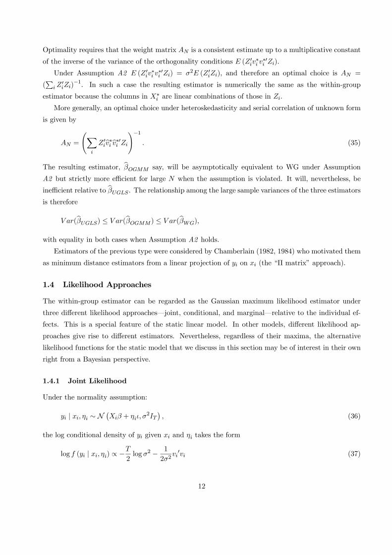
Optimality requires that the weight matrix AN is a consistent estimate up to a multiplicative constant

of the inverse of the variance of the orthogonality conditions E (Z 0iv∗i v∗0i Zi).

Under Assumption A2 E (Z 0iv∗i v∗0i Zi) = σ2E (Z 0iZi), and therefore an optimal choice is AN =

(Pi Z

0iZi)

−1. In such a case the resulting estimator is numerically the same as the within-group

estimator because the columns in X∗i are linear combinations of those in Zi.

More generally, an optimal choice under heteroskedasticity and serial correlation of unknown form

is given by

AN =

ÃXi

Z 0ibv∗i bv∗0i Zi!−1

. (35)

The resulting estimator, bβOGMM say, will be asymptotically equivalent to WG under Assumption

A2 but strictly more efficient for large N when the assumption is violated. It will, nevertheless, be

inefficient relative to bβUGLS . The relationship among the large sample variances of the three estimatorsis therefore

V ar(bβUGLS) ≤ V ar(bβOGMM) ≤ V ar(bβWG),

with equality in both cases when Assumption A2 holds.

Estimators of the previous type were considered by Chamberlain (1982, 1984) who motivated them

as minimum distance estimators from a linear projection of yi on xi (the “Π matrix” approach).

1.4 Likelihood Approaches

The within-group estimator can be regarded as the Gaussian maximum likelihood estimator under

three different likelihood approaches–joint, conditional, and marginal–relative to the individual ef-

fects. This is a special feature of the static linear model. In other models, different likelihood ap-

proaches give rise to different estimators. Nevertheless, regardless of their maxima, the alternative

likelihood functions for the static model that we discuss in this section may be of interest in their own

right from a Bayesian perspective.

1.4.1 Joint Likelihood

Under the normality assumption:

yi | xi, ηi ∼ N¡Xiβ + ηiι,σ

2IT¢, (36)

the log conditional density of yi given xi and ηi takes the form

log f (yi | xi, ηi) ∝ −T

2log σ2 − 1

2σ2vi0vi (37)

12

where vi = (yi −Xiβ − ηiι). Thus, the log likelihood of a cross-sectional sample of independent

observations is a function of β, σ2, and η1, ..., ηN :

L¡β,σ2, η; y, x

¢=

NXi=1

log f (yi | xi, ηi) . (38)

In view of our previous discussion and standard linear regression maximum likelihood (ML) esti-

mation, joint maximization of (38) with respect to β, η, and σ2 yields the WG estimator for β, the

residual estimates for η given in (21), and the residual variance without degrees of freedom correction

for σ2:

eσ2 = 1

NT

NXi=1

bvi0bvi (39)

where bvi = ³yi −XibβWG − bηiι´.Unlike (24) eσ2 will not be a consistent estimator of σ2 for large N and small T panels. In effect,

since E³PN

i=1 bvi0bvi´ = (NT −N − k)σ2, we haveplimN→∞

eσ2 = (T − 1)T

σ2.

Thus eσ2 has a negative (cross-sectional) large sample bias given by σ2/T . This is an example of the

incidental parameter problem studied by Neyman and Scott (1948). The problem is that the maximum

likelihood estimator need not be consistent when the likelihood depends on a subset of (incidental)

parameters whose number increases with sample size. In our case, the likelihood depends on β, σ2

and the incidental parameters η1, ..., ηN . The ML estimator of β is consistent but that of σ2 is not.

1.4.2 Conditional Likelihood

In the linear static model, yi = T−1PT

t=1 yit is a sufficient statistic for ηi. This means that the density

of yi given xi, ηi, and yi does not depend on ηi

f (yi | xi, ηi, yi) = f (yi | xi, yi) . (40)

To see this, note that, expressing the conditional density of yi given yi as a ratio of the joint and

marginal densities, we have

f (yi | xi, ηi, yi) =f (yi | xi, ηi)f (yi | xi, ηi)

and that under (36)

yi | xi, ηi ∼ Nµx0iβ + ηi,

σ2

T

¶,

13

so that

log f (yi | xi, ηi) ∝ −1

2log σ2 − T

2σ2v2i . (41)

Subtracting (41) from (37) we obtain:

log f (yi | xi, ηi, yi) ∝ −(T − 1)2

log σ2 − 1

2σ2

TXt=1

(vit − vi)2 , (42)

which does not depend on ηi because it is only a function of the within-group errors.

Thus the conditional log likelihood

Lc¡β,σ2; y, x

¢=

NXi=1

log f (yi | xi, yi) (43)

is a function of β and σ2, which can be used as an alternative basis for inference. The maximizers of

(43) are the WG estimator of β and

σ2 =1

N(T − 1)NXi=1

bvi0bvi. (44)

Note that contrary to (39), (44) is consistent for large N and small T , although it is not exactly

unbiased as (24).

1.4.3 Marginal (or Integrated) Likelihood

Finally, we may consider the marginal distribution of yi given xi but not ηi:

f (yi | xi) =Zf (yi | xi, ηi) dF (ηi | xi)

where F (ηi | xi) denotes the conditional cdf of ηi given xi. One possibility, in the spirit of the GMMapproach discussed in the previous section, is to assume

ηi | xi ∼ N¡δ + λ0xi,σ2η

¢, (45)

but it is of some interest to study the form of f (yi | xi) for arbitrary F (ηi | xi).Let us consider the non-singular transformation matrix

H =

ÃT−1ι0

A

!. (46)

Note that

f (yi | xi, ηi) = f (Hyi | xi, ηi) |det (H)| , (47)

14

but since |det(H)| = T−1/2 is a constant it can be ignored for our purposes. Moreover, since4

Cov (y∗i , yi | xi, ηi) = 0, (48)

given normality we have that the conditional density of yi factorizes into the between-group and the

orthogonal deviation densities:

f (yi | xi, ηi) = f (yi | xi, ηi) f (y∗i | xi, ηi) . (49)

Note in addition that the orthogonal deviation density is independent of ηi

f (y∗i | xi, ηi) = f (y∗i | xi) ,

and in view of (40) it coincides with the conditional density given yi

f (y∗i | xi) = f (yi | xi, yi) . (50)

Thus, either way we have

log f (yi | xi) = log f (y∗i | xi) + logZf (yi | xi, ηi) dF (ηi | xi) . (51)

If F (ηi | xi) is unrestricted, the second term on the right-hand side of (51) is uninformative about

β so that the marginal ML estimators of β and σ2 coincide with the maximizers ofPNi=1 log f (y

∗i | xi),

which are again given by the WG estimator and (44). This is still true when F (ηi | xi) is specified tobe Gaussian with unrestricted linear projection of ηi on xi, as in (45), but not when ηi is assumed to

be independent of xi (i.e. λ = 0), as we shall see in the next section.

4Note that

Cov (y∗i , yi | xi, ηi) = E (v∗i vi | xi, ηi) = AE viv0i | xi, ηi ι/T = σ2Aι/T = 0.

15

2 Error Components

The analysis in the previous section was motivated by the desire of identifying regression coefficients

that are free from unobserved cross-sectional heterogeneity bias. Another major motivation for using

panel data is the possibility of separating out permanent from transitory components of variation.

2.1 A Variance Decomposition

The starting point of our discussion is a simple variance-components model of the form

yit = μ+ ηi + vit (52)

where μ is an intercept, ηi ∼ iid(0,σ2η), vit ∼ iid(0,σ2), and ηi and vit are independent of each other.

The cross-sectional variance of yit in any given period is given by (σ2η+σ2). This model tells us that a

fraction σ2η/(σ2η + σ2) of the total variance corresponds to differences that remain constant over time

while the rest are differences that vary randomly over time and units.

Dividing total variance into two components that are either completely fixed or completely random

will often be unrealistic, but this model and its extensions are at the basis of much useful econometric

descriptive work. A prominent example is the study of earnings inequality and mobility (cf. Lillard

and Willis, 1978). In the analysis of transitions between log-normal earnings classes, the model allows

us to distinguish between aggregate or unconditional transition probabilities and individual transition

probabilities given certain values of permanent characteristics represented by ηi.

Indeed, given ηi, the ys are independent over time but with different means for different units, so

that we have

yi | ηi ∼ id¡(μ+ ηi)ι,σ

2IT¢,

whereas unconditionally we have

yi ∼ iid(μι,Ω)

with

Ω = σ2IT + σ2ηιι0. (53)

Thus the unconditional correlation between yit and yis for any two periods t 6= s is given by

Corr(yit, yis) =σ2η

σ2η + σ2=

λ

1 + λ(54)

with λ = σ2η/σ2.

16

Estimating the Variance-Components Model One possibility is to approach estimation

conditionally given the ηi. That is, to estimate the realizations of the permanent effects that occur in

the sample and σ2. Natural unbiased estimates in this case would be

bηi = yi − y (i = 1, ...,N) (55)

and

bσ2 = 1

N(T − 1)NXi=1

TXt=1

(yit − yi)2 , (56)

where yi = T−1PT

t=1 yit and y = N−1PN

i=1 yi. However, typically both σ2η and σ

2 will be parameters

of interest. To obtain an estimator of σ2η note that the variance of yi is given by

V ar(yi) ≡ σ2 = σ2η +σ2

T. (57)

Therefore, a large-N consistent estimator of σ2η can be obtained as the difference between the estimated

variance of yi and bσ2/T :bσ2η = 1

N

NXi=1

(yi − y)2 −bσ2T. (58)

A problem with this estimator is that it is not guaranteed to be non-negative by construction.

The statistics (56) and (58) can be regarded as Gaussian ML estimates under yi ∼ N (μι,Ω). Tosee this, note that using transformation (46) in general we have:

Hyi =

Ãyi

y∗i

!∼ id

"Ãμ

0

!,

Ãσ2 0

0 σ2IT−1

!#. (59)

Hence, under normality the log density of yi can be decomposed as

log f (yi) = log f (yi) + log f (y∗i ) , (60)

so that the log likelihood of (y1, ..., yN) is given by

L(μ,σ2,σ2) = LB(μ,σ2) + LW (σ

2), (61)

where

LB(μ,σ2) ∝ −N

2log σ2 − 1

2σ2

NXi=1

(yi − μ)2 (62)

and

LW (σ2) ∝ −N(T − 1)

2log σ2 − 1

2σ2

NXi=1

y∗0i y∗i . (63)

17

Clearly the ML estimates of σ2 and σ2 are given by (56) and the sample variance of yi, respectively.5

Moreover, the ML estimator of σ2η is given by (58) in view of the invariance property of maximum

likelihood estimation.

Note that with large N and short T we can obtain precise estimates of σ2η and σ2 but not of the

individual realizations ηi. Conversely, with small N and large T we would be able to obtain accurate

estimates of ηi and σ2 but not of σ2η, the intuition being that although we can estimate the individual

ηi well there may be too few of them to obtain a good estimate of their variance.

For large N , σ2η is just-identified when T = 2 in which case we have σ2η = Cov(yi1, yi2).

6

2.2 Error-Components Regression

2.2.1 The Model

Often one is interested in the analysis of error-components models given some conditioning variables.

The conditioning variables may be time-varying, time-invariant or both, denoted as xit and fi, respec-

tively. For example, we may be interested in separating out permanent and transitory components of

individual earnings by labour market experience and educational categories.

This gives rise to a regression version of the previous model in which, in principle, not only μ

but also σ2η and σ2 could be functions of xit and fi. Nevertheless, in the standard error-components

regression model μ is period-specific and made a linear function of xit and fi, while the variance

parameters are assumed not to vary with the regressors. The model is therefore

yit = x0itβ + f0iγ + uit (64)

uit = ηi + vit (65)

together with the following assumption for the composite vector of errors ui = (ui1, ..., uiT )0:

ui | wi ∼ iid(0,σ2IT + σ2ηιι0) (66)

where wi = (x0i1, ..., x0iT , f

0i)0.

This model is similar to the one discussed in the previous chapter except in one fundamental

aspect. The individual effect in the unobserved-heterogeneity model was potentially correlated with

xit. Indeed, this was the motivation for considering such a model in the first place. In contrast, in

the error-components model ηi and vit are two components of a regression error and hence both are

uncorrelated with the regressors.

Formally, this model is a specialization of the unobserved-heterogeneity model of the previous

chapter under Assumptions A1 and A2 in which in addition

E(ηi | wi) = 0 (67)

5Note that Ni=1 y

∗0i y

∗i =

Ni=1

Tt=1 (yit − yi)2.

6With T = 2, (58) coincides with the sample covariance between yi1 and yi2.

18

V ar(ηi | wi) = σ2η. (68)

To reconcile the notation used in the two instances, note that in the unobserved heterogeneity

model, the time-invariant component of the regression f 0iγ is subsumed under the individual effect

ηi. Moreover, in the unobserved-heterogeneity model we did not specify an intercept so that E(ηi)

was not restricted, whereas for the error-components model E(ηi) = 0, and fi will typically contain a

constant term.

Note that in the error-components model β is identified in a single cross-section. The parameters

that require panel data for identification in this model are the variances of the components of the error

σ2η and σ2, which typically will be parameters of central interest in this context.

There are also applications of model (64)-(65) in which the main interest lies in the estimation of

β and γ. In these cases it is natural to regard the error-components model as a restrictive version of

the unobserved heterogeneity model of Section 1 with uncorrelated individual effects.

2.2.2 GLS and ML Estimation

Under the previous assumptions, OLS in levels provides unbiased and consistent but inefficient esti-

mators of β and γ:

bδOLS = Ã NXi=1

W 0iWi

!−1 NXi=1

W 0iyi (69)

where Wi =

µXi...ιf 0i

¶, Xi = (xi1, ..., xiT )

0, and δ =¡β0, γ0

¢0.Optimal estimation is achieved through GLS, also known as the Balestra—Nerlove estimator:7

bδGLS = Ã NXi=1

W 0iΩ−1Wi

!−1 NXi=1

W 0iΩ−1yi. (70)

This GLS estimator is, nevertheless, unfeasible, since Ω depends on σ2η and σ2, which are unknown.

Feasible GLS is obtained by replacing them by consistent estimates. Usually, the following are used:

bσ2 = 1

N(T − 1)− kNXi=1

TXt=1

³eyit − ex0itbβWG

´2(71)

bσ2η = 1

N

NXi=1

³yi − w0ibδBG´2 − bσ2T (72)

where eyit = yit − yi, exit = xit − xi, and bδBG denotes the between-group estimator, which is given bythe OLS regression of yi on wi:

bδBG = Ã NXi=1

wiw0i

!NXi=1

wiyi. (73)

7cf. Balestra and Nerlove (1966).

19

Alternatively, the full set of parameters β, γ, σ2, and σ2η may be jointly estimated by maximum

likelihood. As in the case without regressors, the log likelihood can be decomposed as the sum of the

between and within log likelihoods. In this case we have:Ãyi

y∗i

!| wi ∼ id

"Ãx0iβ + f

0iγ

X∗i β

!,

Ãσ2 0

0 σ2IT−1

!#, (74)

so that under normality the error-components log likelihood equals:

L¡β, γ,σ2,σ2

¢= LB

¡β, γ,σ2

¢+ LW

¡β,σ2

¢(75)

where

LB¡β, γ,σ2

¢ ∝ −N2log σ2 − 1

2σ2

NXi=1

¡yi − x0iβ − f 0iγ

¢2 (76)

and

LW¡β,σ2

¢ ∝ −N(T − 1)2

log σ2 − 1

2σ2

NXi=1

(y∗i −X∗i β)0 (y∗i −X∗i β) . (77)

Separate maximization of LW and LB gives rise to within-group and between group estimation,

respectively. Thus, the error-components likelihood can be regarded as enforcing the restriction that

the parameter vectors β that appear in LW and LB coincide. This immediately suggests a (likelihood-

ratio) specification test that will be further discussed below.

Moreover, in the absence of individual effects σ2η = 0 so that σ2 = σ2/T . Thus, the OLS estimator in

levels (69) can be regarded as the MLE that maximizes the log-likelihood (75) subject to the restriction

σ2 = σ2/T . Again, this suggests a likelihood-ratio (LR) test of the existence of (uncorrelated) effects

based on the comparison of the restricted and unrestricted likelihoods. Such a test will, nevertheless,

be sensitive to distributional assumptions.

In terms of the transformed model, bδGLS can be written as a weighted least-squares estimator:bδGLS = " NX

i=1

¡W ∗0i W

∗i + φ2wiw

0i

¢#−1 NXi=1

¡W ∗0i y

∗i + φ2wiyi

¢(78)

where φ2 is the ratio of the within to the between error variances φ2 = σ2/σ2, W ∗i = AWi, and

wi = T−1W 0i ι. Thus bδGLS can be regarded as a matrix-weighted average of the within-group and

between-group estimators (Maddala, 1971). The statistic (78) is identical to (70).8 For feasible GLS,

φ2 is replaced by the ratio of the within to the between sample residual variances bφ2 = bσ2/bσ2.So far we have motivated error-components regression models from a direct interest in the com-

ponents themselves. Sometimes, however, correlation between individual effects and regressors can be

regarded as an empirical issue. Next we address the testing of such hypothesis.8When φ2 = T (or σ2η = 0) (78) boils down to the OLS in levels estimator (69), whereas if σ

2η →∞ then φ2 → 0 and

δGLS tends to within-groups.

20

2.3 Testing for Correlated Unobserved Heterogeneity

Sometimes correlated unobserved heterogeneity is a basic property of the model of interest. An

example is a “λ-constant” labour supply equation where ηi is determined by the marginal utility of

initial wealth, which according to the underlying life-cycle model will depend on wages in all periods

(MaCurdy, 1981). Another example is when a regressor is a lagged dependent variable. In cases like

this, testing for lack of correlation between regressors and individual effects is not warranted since we

wish the model to have this property.

On other occasions, correlation between regressors and individual effects can be regarded as an

empirical issue. In these cases testing for correlated unobserved heterogeneity can be a useful specifi-

cation test for regression models estimated in levels. Researchers may have a preference for models in

levels because estimates in levels are in general more precise than estimates in deviations (dramatically

so when the time series variation in the regressors relative to the cross-sectional variation is small), or

because of an interest in regressors that lack time series variation.

2.3.1 Specification Tests

We have already suggested a specification test of correlated effects from a likelihood ratio perspective.

This was a test of equality of the β coefficients appearing in the WG and BG likelihoods. Similarly,

from a least-squares perspective, we may consider the system

yi = x0ib+ f

0ic+ εi (79)

y∗i = X∗i β + u

∗i , (80)

where b, c, and εi are such that E∗(εi | xi, fi) = 0, and formulate the problem as a (Wald) test of the

null hypothesis9

H0 : β = b. (81)

The least-squares perspective is of interest because it can easily accommodate robust generaliza-

tions to heteroskedasticity and serial correlation.

Under the unobserved-heterogeneity model

E(yi | wi) = x0iβ + f 0iγ +E(ηi | wi),

so that (79) can be regarded as a specification of an alternative hypothesis of the form

H1 : E(ηi | wi) = x0iλ1 + f 0iλ2 (82)

with b = β+ λ1 and c = γ + λ2. H0 is, therefore, equivalent to λ1 = 0. Note that H0 does not specify

that λ2 = 0, which is not testable.9Under the assumptions of the error-components model b = β, c = γ, and εi = ui.

21

Under (82) and the additional assumption V ar(ηi | wi) = σ2η, the error covariance matrix of the

system (79)-(80) is given by V ar (εi | wi) = σ2, Cov (εi, u∗i | wi) = 0, and V ar (u∗i | wi) = σ2IT−1.

Thus the optimal LS estimates of (b0, c0)0 and β are the BG and the WG estimators, respectively.

Explicit expressions for the BG estimator of b and its estimated variance matrix are:

bbBG = ³X 0MX

´−1X0My (83)

bVBG ≡ dV ar ³bbBG´ = bσ2 ³X 0MX

´−1(84)

where M = I − F (F 0F )−1 F 0, F = (f1, ..., fN)0, X = (x1, ..., xN )0, and y = (y1, ..., yN)

0. Likewise, the

estimated variance matrix of the WG estimator is

bVWG ≡ dV ar ³bβWG

´= bσ2µXN

i=1X∗

0i X

∗i

¶−1. (85)

Moreover, since Cov³bbBG, bβWG

´= 0, the Wald test of (81) is given by

h =³bbBG − bβWG

´0(bVWG + bVBG)−1 ³bbBG − bβWG

´. (86)

Under H0, the statistic h will have a χ2 distribution with k degrees of freedom in large samples.

Clearly, h will be sensitive to the nature of the variables included in fi. For example, H0 might be

rejected when fi only contains a constant term, but not when a larger set of time-invariant regressors

is included.

Hausman (1978) originally motivated the testing of correlated effects as a comparison between WG

and the Balestra—Nerlove GLS estimator, suggesting a statistic of the form

h =³bβGLS − bβWG

´0(bVWG − bVGLS)−1 ³bβGLS − bβWG

´, (87)

where

bVGLS = bσ2(X∗0X∗ + bφ2X 0MX)−1. (88)

Under H0 both estimators are consistent, so we would expect the difference bβGLS − bβWG to be

small. Moreover, since bβGLS is efficient, the variance of the difference must be given by the differenceof variances. Otherwise, we could find a linear combination of the two estimators that would be

more efficient than GLS. Under H1 the WG estimator remains consistent but GLS does not, so their

difference and the test statistic will tend to be large. A statistic of the form given in (87) is known as

a Hausman test statistic. As shown by Hausman and Taylor (1981), (87) is in fact the same statistic

as (86). Thus h can be regarded both as a Hausman test or as a Wald test of the restriction λ1 = 0

from OLS estimates of the model under the alternative.

22

If the errors are heteroskedastic and/or serially correlated, the previous formulae for the large

sample variances of WG, BG, and GLS are not valid. Moreover, WG and GLS cannot be ranked in

terms of efficiency so that the variance of the difference between the two does not coincide with the

difference of variances. Following the Wald approach, Arellano (1993) suggested a generalized test

that is robust to heteroskedasticity and autocorrelation.

+

+ ++

+++

+

+

+

+

+ +

+++

+++ +

η1

η2

η3

η4

x2 x4x3x3x1

between-group line

yit

xit

within-group lines

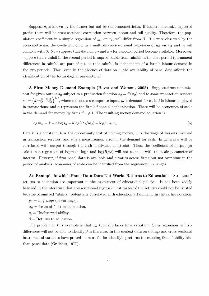
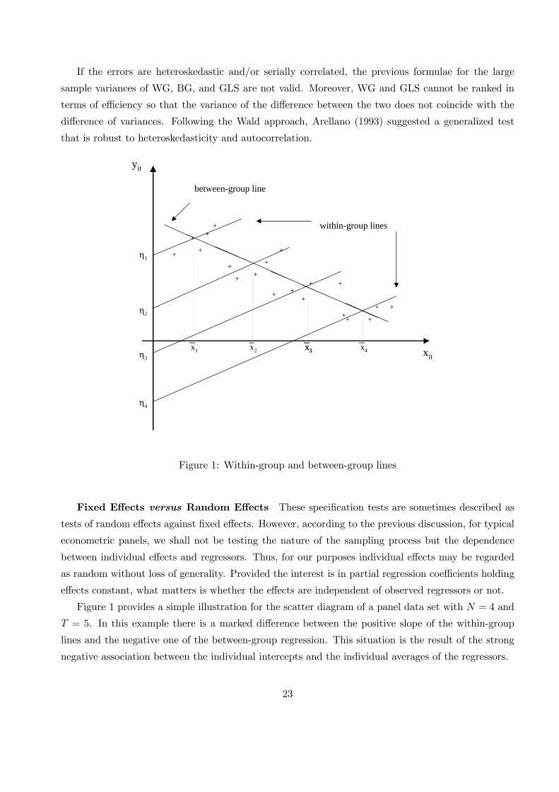
Figure 1: Within-group and between-group lines

Fixed Effects versus Random Effects These specification tests are sometimes described as

tests of random effects against fixed effects. However, according to the previous discussion, for typical

econometric panels, we shall not be testing the nature of the sampling process but the dependence

between individual effects and regressors. Thus, for our purposes individual effects may be regarded

as random without loss of generality. Provided the interest is in partial regression coefficients holding

effects constant, what matters is whether the effects are independent of observed regressors or not.

Figure 1 provides a simple illustration for the scatter diagram of a panel data set with N = 4 and

T = 5. In this example there is a marked difference between the positive slope of the within-group

lines and the negative one of the between-group regression. This situation is the result of the strong

negative association between the individual intercepts and the individual averages of the regressors.

23

2.3.2 Robust GMM Estimation and Testing

Under the null of uncorrelated effects we may consider GMM estimation based on the orthogonality

conditions10

E£xi¡yi − x0iβ − f 0iγ

¢¤= 0 (89)

E£fi¡yi − x0iβ − f 0iγ

¢¤= 0 (90)

E [(y∗i −X∗i β)⊗ xi] = 0. (91)

In parallel with the development in Section 1.3.3, the resulting estimates of β and γ will be

asymptotically equivalent to Balestra—Nerlove GLS with classical errors, but strictly more efficient

when heteroskedasticity or autocorrelation is present. However, under the alternative of correlated

effects, any GMM estimate that relies on the moments (89) will be inconsistent for β. Thus, we may

test for correlated effects by considering an incremental test of the over identifying restrictions (89).

Note that under the alternative, GMM estimates based on (90)-(91) will be consistent for β but not

necessarily for γ.

Optimal GMM estimates in this context minimize a criterion of the form

s(δ) =

"NXi=1

(yi −Wiδ)H0Zi

#ÃNXi=1

Z 0iHbuibu0iH 0Zi

!−1 " NXi=1

Z 0iH(yi −Wiδ)

#(92)

where Hbui are some one-step consistent residuals. Under uncorrelated effects the instrument matrixZi takes the form

Zi =

Ãx0i f 0i 0

0 0 IT−1 ⊗ x0i

!, (93)

whereas under correlated effects we shall use

Zi =

Ãf 0i 0

0 IT−1 ⊗ x0i

!. (94)

10We could also add:

E [(y∗i −X∗i β)⊗ fi] = 0,

in which case, the entire set of moments can be expressed in terms of the original equation system as:

E yi −Xiβ − ιf 0iγ ⊗ wi = 0.

When fi contains a constant term only, this amounts to including a set of time dummies in the instrument set.

24

2.4 Models with Information in Levels

Sometimes it is of central interest to measure the effect of a time-invariant explanatory variable

controlling for unobserved heterogeneity. Returns to schooling holding unobserved ability constant

is a prominent example. In those cases, as explained in Section 1, panel data is not directly useful.

Hausman and Taylor (1981) argued, however, that panel data might still be useful in an indirect way

if the model contained time-varying explanatory variables that were uncorrelated with the effects.

Suppose there are subsets of the time-invariant and time-varying explanatory variables, f1i and

x1i = (x01i1, ..., x

01iT )

0 respectively, that can be assumed a priori to be uncorrelated with the effects. In

such case, the following subset of the orthogonality conditions (89)-(91) hold

E£x1i¡yi − x0iβ − f 0iγ

¢¤= 0 (95)

E£f1i¡yi − x0iβ − f 0iγ

¢¤= 0 (96)

E [(y∗i −X∗i β)⊗ xi] = 0. (97)

The parameter vector β will be identified from the moments for the errors in deviations (97). The

basic point noted by Hausman and Taylor is that the coefficients γ may also be identified using the

variables x1i and f1i as instruments for the errors in levels, provided the rank condition is satisfied.

Given identification, the coefficients β and γ can be estimated by GMM (Arellano and Bover, 1995).

The notion that a time-varying variable that is uncorrelated with an individual effect can be used

at the same time as an instrument for itself and for a correlated time-invariant variable is potentially

appealing. Nevertheless, the impact of these models in applied work has been limited, due to the

difficulty in finding exogenous variables that can be convincingly regarded a priori as being uncorrelated

with the individual effects.

25

3 Error in Variables

3.1 Introduction to the Standard Regression Model with Errors in Variables

Let us consider a cross-sectional regression model

yi = α+ x†iβ + vi. (98)

Suppose we actually observe yi and xi, which is a noisy measure of x†i subject to an additive

measurement error εi

xi = x†i + εi. (99)

We assume that all the unobservables x†i , vi, and εi are mutually independent with variances σ2†,

σ2v, and σ2ε. Since vi is independent of x†i , β is given by the population regression coefficient of yi on

x†i :

β =Cov(yi, x

†i )

V ar(x†i ), (100)

but since x†i is unobservable we cannot use a sample counterpart of this expression as an estimator of

β.

What do we obtain by regressing yi on xi in the population? The result is

Cov(yi, xi)

V ar(xi)=Cov(yi, x

†i + εi)

σ2† + σ2ε=Cov(yi, x

†i )

σ2† + σ2ε=

β

1 + λ(101)

where λ = σ2ε/σ2†. Note that since λ is non-negative by construction, the population regression

coefficient of yi on xi will always be smaller than β in absolute value as long as σ2ε > 0.

This type of model is relevant in at least two conceptually different situations. One corresponds to

instances of actual measurement errors due to misreporting, rounding-off errors, etc. The other arises

when the variable of economic interest is a latent variable which does not correspond exactly to the

one that is available in the data.

In either case, the worry is that the variable to which agents respond does not coincide with the

one that is entered as a regressor in the model. The result is that the unobservable component in

the relationship between yi and xi will contain a multiple of the measurement error in addition to the

error term in the original relationship:

yi = α+ xiβ + ui (102)

ui = vi − βεi. (103)

Clearly, the observed regressor xi will be correlated with ui even if the latent variable x†i is not.

26

This problem is often of practical significance, specially in regression analysis with micro data,

since the resulting biases may be large. Note that the magnitude of the bias does not depend on

the absolute magnitude of the measurement error variance but on the “noise to signal” ratio λ. For

example, if λ = 1, so that 50 per cent of the total variance observed in xi is due to measurement

error–which is not an uncommon situation–the population regression coefficient of yi on xi will be

half the value of β.

As for solutions, suppose we have the means of assessing the extent of the measurement error, so

that λ or σ2ε are known or can be estimated. Then β can be determined as

β = (1 + λ)Cov(yi, xi)

V ar(xi)=

Cov(yi, xi)

V ar(xi)− σ2ε. (104)

More generally, in a model with k regressors and a conformable vector of coefficients β

yi = x0iβ +

¡vi − ε0iβ

¢(105)

with E(εiε0i) = Ωε, E(x†ix†0i ) = Ω† and Λ = Ω

−1† Ωε:

β = (Ik + Λ)£E(xix

0i)¤−1

E(xiyi) =£E(xix

0i)−Ωε

¤−1E(xiyi). (106)

In this notation, xi will include a constant term, and possibly other regressors without measurement

error. This situation will be reflected by the occurrence of zeros in the corresponding elements of Ωε.

The expression (106) suggests an estimator of the form

eβ = Ã 1N

NXi=1

xix0i − eΩ−1ε

!1

N

NXi=1

xiyi. (107)

where eΩε denotes a consistent estimate of Ωε.

Alternatively, if we have a second noisy measure of x†i

zi = x†i + ζi (108)

such that the measurement error ζi is independent of εi and the other unobservables, it can be used

as an instrumental variable. In effect, for scalar xi we have

Cov(zi, yi)

Cov(zi, xi)=

Cov(x†i + ζi, yi)

Cov(x†i + ζi, x†i + εi)

=Cov(yi, x

†i )

V ar(x†i )= β. (109)

Moreover, since also

Cov(xi, yi)

Cov(xi, zi)= β, (110)

there is one overidentifying restriction in this problem.

27

In some way the instrumental variable solution is not different from the previous one. Indirectly, the

availability of two noisy measures is used to identify the systematic and measurement error variances.

Note that since

V ar

Ãxi

zi

!=

Ãσ2† + σ2ε σ2†

σ2† σ2† + σ2ζ

!(111)

we can determine the variances of the unobservables as

σ2† = Cov(zi, xi) (112)

σ2ε = V ar(xi)− Cov(zi, xi) (113)

σ2ζ = V ar(zi)− Cov(zi, xi). (114)

In econometrics the instrumental variable approach is the most widely used technique. Thus, the

response to measurement error bias in linear regression problems is akin to the response to simultaneity

bias. This similarity, however, no longer holds in the nonlinear regression context. The problem is

that in a nonlinear regression the measurement error is no longer additively separable from the true

value of the regressor.

3.2 Measurement Error Bias and Unobserved Heterogeneity Bias

Let us consider a cross-sectional model that combines measurement error and unobserved heterogeneity

yi = x†iβ + ηi + vi (115)

xi = x†i + εi,

where all unobservables are independent, except x†i and ηi. The population regression coefficient of yion xi is given by

Cov(yi, xi)

V ar(xi)= β +

Cov(ηi + vi − βεi, xi)

V ar(xi)= β −

Ãσ2ε

σ2† + σ2ε

!β +

ÃCov(ηi, x

†i )

σ2† + σ2ε

!. (116)

Note that there are two components to the bias. The first one is due to measurement error and

depends on σ2ε. The second is due to unobserved heterogeneity and depends on Cov(ηi, x†i ). Sometimes

these two biases tend to offset each other. For example, if β > 0 and Cov(ηi, x†i ) > 0, the measurement

error bias will be negative while the unobserved heterogeneity bias will be positive. A full offsetting

would only occur if Cov(ηi, x†i ) = σ2εβ, something that could only happen by chance.

28

Measurement Error Bias in First-Differences Suppose we have panel data with T = 2 and

consider a regression in first-differences as a way of removing unobserved heterogeneity bias. In such

a case we obtain

Cov(∆yi2,∆xi2)

V ar(∆xi2)=

β

1 + λ∆(117)

where λ∆ = V ar(∆εi2)/V ar(∆x†i2).

The main point to make here is that first-differencing may exacerbate the measurement error bias.

The reason is as follows. If εit is an iid error then V ar(∆εi2) = 2σ2ε. If x†it is also iid then λ∆ = λ, and

the measurement error bias in levels and first-differences will be of the same magnitude. However, if

x†it is a stationary time series with positive serial correlation

V ar(∆x†i2) = 2hσ2† − Cov(x†i1, x†i2)

i< 2σ2† (118)

and therefore λ∆ > λ.11

A related example of this situation in data with a group structure arises in the analysis of the

returns to schooling with data on twin siblings. Regressions in differences remove genetic ability

bias but may exacerbate measurement error bias in schooling if the siblings’ measurement errors are

independent but their true schooling attainments are highly correlated (Griliches, 1977).

Under the same circumstances, the within-group measurement error bias with T > 2 will be

smaller than that in first-differences but higher than the measurement error bias in levels (Griliches

and Hausman, 1986).

Therefore, the finding of significantly different results in regressions in first-differences and orthog-

onal deviations may be an indication of the presence of measurement error.

3.3 Instrumental Variable Estimation with Panel Data

The availability of panel data helps to solve the problem of measurement error bias by providing

internal instruments as long as we are willing to restrict the serial dependence in the measurement

error.

In a model without unobserved heterogeneity the following orthogonality conditions are valid pro-

11Note that, as explained in Section 2, the cross-sectional covariance between x†i1 and x†i2 will also be positive in the

presence of heterogeneity, even if the individual time series are not serially correlated.

29

vided the measurement error is white noise and T ≥ 2:

E[

⎛⎜⎜⎜⎜⎜⎜⎜⎜⎜⎜⎜⎜⎜⎝

1

xi1...

xi(t−1)xi(t+1)...

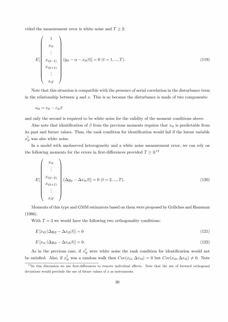
xiT

⎞⎟⎟⎟⎟⎟⎟⎟⎟⎟⎟⎟⎟⎟⎠(yit − α− xitβ)] = 0 (t = 1, ..., T ). (119)

Note that this situation is compatible with the presence of serial correlation in the disturbance term

in the relationship between y and x. This is so because the disturbance is made of two components:

uit = vit − εitβ

and only the second is required to be white noise for the validity of the moment conditions above.

Also note that identification of β from the previous moments requires that xit is predictable from

its past and future values. Thus, the rank condition for identification would fail if the latent variable

x†it was also white noise.

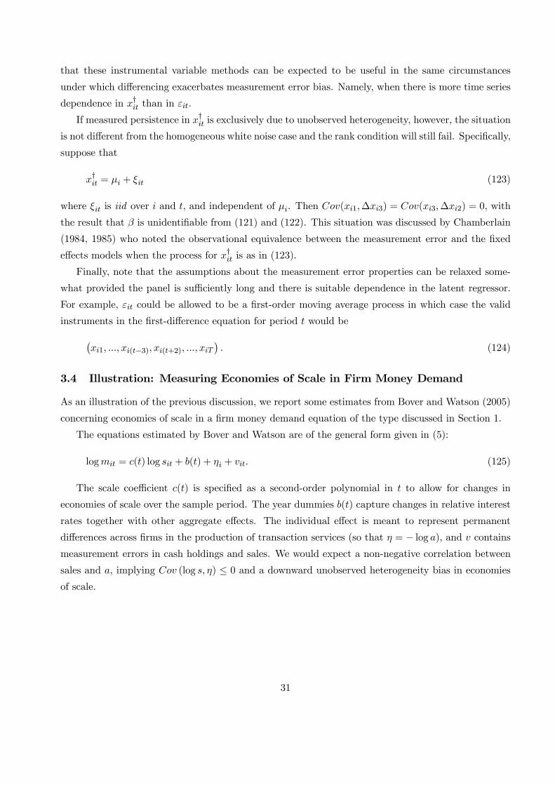
In a model with unobserved heterogeneity and a white noise measurement error, we can rely on

the following moments for the errors in first-differences provided T ≥ 3:12

E[

⎛⎜⎜⎜⎜⎜⎜⎜⎜⎜⎜⎜⎝

xi1...

xi(t−2)xi(t+1)...

xiT

⎞⎟⎟⎟⎟⎟⎟⎟⎟⎟⎟⎟⎠(∆yit −∆xitβ)] = 0 (t = 2, ..., T ). (120)

Moments of this type and GMM estimators based on them were proposed by Griliches and Hausman

(1986).

With T = 3 we would have the following two orthogonality conditions:

E [xi3 (∆yi2 −∆xi2β)] = 0 (121)

E [xi1 (∆yi3 −∆xi3β)] = 0. (122)

As in the previous case, if x†it were white noise the rank condition for identification would not

be satisfied. Also, if x†it was a random walk then Cov(xi1,∆xi3) = 0 but Cov(xi3,∆xi2) 6= 0. Note

12 In this discussion we use first-differences to remove individual effects. Note that the use of forward orthogonal

deviations would preclude the use of future values of x as instruments.

30

that these instrumental variable methods can be expected to be useful in the same circumstances

under which differencing exacerbates measurement error bias. Namely, when there is more time series

dependence in x†it than in εit.

If measured persistence in x†it is exclusively due to unobserved heterogeneity, however, the situation

is not different from the homogeneous white noise case and the rank condition will still fail. Specifically,

suppose that

x†it = μi + ξit (123)

where ξit is iid over i and t, and independent of μi. Then Cov(xi1,∆xi3) = Cov(xi3,∆xi2) = 0, with

the result that β is unidentifiable from (121) and (122). This situation was discussed by Chamberlain

(1984, 1985) who noted the observational equivalence between the measurement error and the fixed

effects models when the process for x†it is as in (123).

Finally, note that the assumptions about the measurement error properties can be relaxed some-

what provided the panel is sufficiently long and there is suitable dependence in the latent regressor.

For example, εit could be allowed to be a first-order moving average process in which case the valid

instruments in the first-difference equation for period t would be¡xi1, ..., xi(t−3), xi(t+2), ..., xiT

¢. (124)

3.4 Illustration: Measuring Economies of Scale in Firm Money Demand

As an illustration of the previous discussion, we report some estimates from Bover and Watson (2005)

concerning economies of scale in a firm money demand equation of the type discussed in Section 1.

The equations estimated by Bover and Watson are of the general form given in (5):

logmit = c(t) log sit + b(t) + ηi + vit. (125)

The scale coefficient c(t) is specified as a second-order polynomial in t to allow for changes in

economies of scale over the sample period. The year dummies b(t) capture changes in relative interest

rates together with other aggregate effects. The individual effect is meant to represent permanent

differences across firms in the production of transaction services (so that η = − log a), and v containsmeasurement errors in cash holdings and sales. We would expect a non-negative correlation between

sales and a, implying Cov (log s, η) ≤ 0 and a downward unobserved heterogeneity bias in economiesof scale.

31

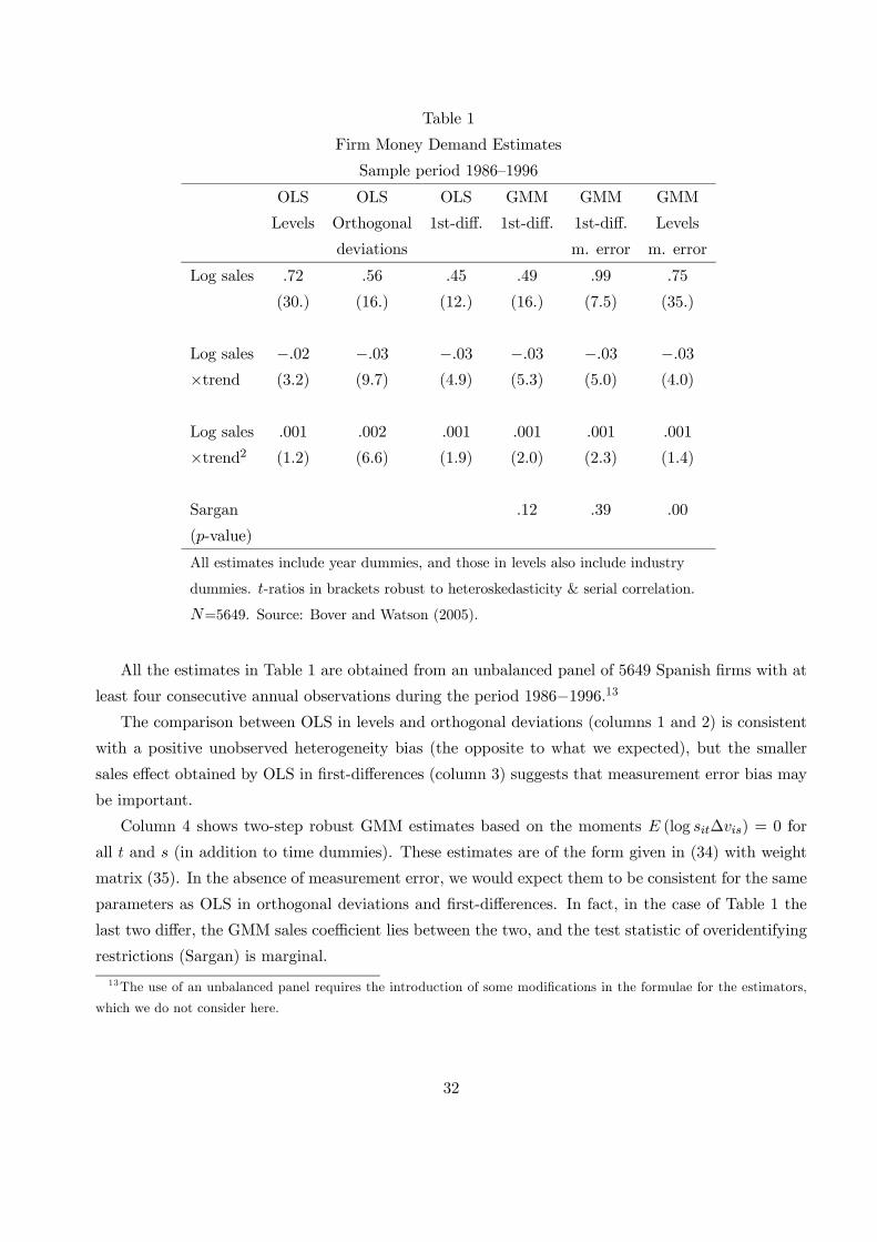
Table 1

Firm Money Demand Estimates

Sample period 1986—1996

OLS OLS OLS GMM GMM GMM

Levels Orthogonal 1st-diff. 1st-diff. 1st-diff. Levels

deviations m. error m. error

Log sales .72 .56 .45 .49 .99 .75

(30.) (16.) (12.) (16.) (7.5) (35.)

Log sales −.02 −.03 −.03 −.03 −.03 −.03×trend (3.2) (9.7) (4.9) (5.3) (5.0) (4.0)

Log sales .001 .002 .001 .001 .001 .001

×trend2 (1.2) (6.6) (1.9) (2.0) (2.3) (1.4)

Sargan .12 .39 .00

(p-value)

All estimates include year dummies, and those in levels also include industry

dummies. t-ratios in brackets robust to heteroskedasticity & serial correlation.

N=5649. Source: Bover and Watson (2005).

All the estimates in Table 1 are obtained from an unbalanced panel of 5649 Spanish firms with at

least four consecutive annual observations during the period 1986−1996.13The comparison between OLS in levels and orthogonal deviations (columns 1 and 2) is consistent

with a positive unobserved heterogeneity bias (the opposite to what we expected), but the smaller

sales effect obtained by OLS in first-differences (column 3) suggests that measurement error bias may

be important.

Column 4 shows two-step robust GMM estimates based on the moments E (log sit∆vis) = 0 for

all t and s (in addition to time dummies). These estimates are of the form given in (34) with weight

matrix (35). In the absence of measurement error, we would expect them to be consistent for the same

parameters as OLS in orthogonal deviations and first-differences. In fact, in the case of Table 1 the

last two differ, the GMM sales coefficient lies between the two, and the test statistic of overidentifying

restrictions (Sargan) is marginal.

13The use of an unbalanced panel requires the introduction of some modifications in the formulae for the estimators,

which we do not consider here.

32

Column 5 shows GMM estimates based on

E (log sit∆vis) = 0 (t = 1, ..., s− 2, s+ 1, .., T ; s = 1, ..., T ), (126)

thus allowing for both correlated firm effects and serially independent multiplicative measurement

errors in sales. Interestingly, now the leading sales coefficient is much higher and close to unity, and

the Sargan test has a p-value close to 40 per cent.

Finally, column 6 shows GMM estimates based on

E (log sitvis) = 0 (t = 1, ..., s− 1, s+ 1, .., T ; s = 1, ..., T ). (127)

In this case, as with the other estimates in levels, firm effects in (125) are replaced by industry effects.

Therefore, the estimates in column 6 allow for serially uncorrelated measurement error in sales but

not for correlated effects. The leading sales effect in this case is close to OLS in levels, suggesting

that in levels the measurement error bias is not as important as in the estimation in differences. The

Sargan test provides a sound rejection, which can be interpreted as a rejection of the null of lack of

correlation between sales and firm effects, allowing for measurement error.

What is interesting about this example is that a comparison between estimates in levels and

deviations without consideration of the possibility of measurement error (e.g. restricted to compare

columns 1 and 2, or 1 and 3, as in Hausman-type testing), would lead to the conclusion of correlated

effects, but with biases going in entirely the wrong direction.

References

[1] Arellano, M. (1987): “Computing Robust Standard Errors for Within-Group Estimators”, Oxford

Bulletin of Economics and Statistics, 49, 431-434.

[2] Arellano, M. (1993): “On the Testing of Correlated Effects with Panel Data”, Journal of Econo-

metrics, 59, 87-97.

[3] Arellano, M. (2003): Panel Data Econometrics, Oxford University Press, Oxford.

[4] Arellano, M. and O. Bover (1995): “Another Look at the Instrumental-Variable Estimation of

Error-Components Models”, Journal of Econometrics, 68, 29-51.

[5] Balestra, P. and M. Nerlove (1966): “Pooling Cross Section and Time Series Data in the Estima-

tion of a Dynamic Model: The Demand for Natural Gas”, Econometrica, 34, 585-612.

[6] Bover, O. and N. Watson (2005): “Are There Economies of Scale in the Demand for Money by

Firms? Some Panel Data Estimates”, Journal of Monetary Economics, 52, 1569-1589.

33

[7] Chamberlain, G. (1982): “Multivariate Regression Models for Panel Data”, Journal of Econo-

metrics, 18, 5-46.

[8] Chamberlain, G. (1984): “Panel Data”, in Griliches, Z. and M.D. Intriligator (eds.), Handbook of

Econometrics, vol. 2, Elsevier Science, Amsterdam.

[9] Chamberlain, G. (1985): “Heterogeneity, Omitted Variable Bias, and Duration Dependence”, in

Heckman, J. J. and B. Singer (eds.), Longitudinal Analysis of Labor Market Data, Cambridge

University Press, Cambridge.

[10] Griliches, Z. (1977): “Estimating the Returns to Schooling: Some Econometric Problems”, Econo-

metrica, 45, 1-22.

[11] Griliches, Z. and J. A. Hausman (1986): “Errors in Variables in Panel Data”, Journal of Econo-

metrics, 31, 93-118.

[12] Hausman, J. A. (1978): “Specification Tests in Econometrics”, Econometrica, 46, 1251-1272.

[13] Hausman, J. A. and W. E. Taylor (1981): “Panel Data an Unobservable Individual Effects”,

Econometrica, 49, 1377-1398.

[14] Hoch, I. (1962): “Estimation of Production Function Parameters Combining Time-Series and

Cross-Section Data”, Econometrica, 30, 34-53.

[15] Kiefer, N. M. (1980): “Estimation of Fixed Effect Models for Time Series of Cross-Sections with

Arbitrary Intertemporal Covariance”, Journal of Econometrics, 14, 195-202.

[16] Lillard, L. and R. J. Willis (1978): “Dynamic Aspects of Earnings Mobility”, Econometrica, 46,

985-1012.

[17] MaCurdy, T. E. (1981): “An Empirical Model of Labor Supply in a Life-Cycle Setting”, Journal

of Political Economy, 89, 1059-1085.

[18] Maddala, G. S. (1971): “The Use of Variance Components Models in Pooling Cross Section and

Time Series Data”, Econometrica, 39, 351-358.

[19] Mundlak, Y. (1961): “Empirical Production Function Free of Management Bias”, Journal of

Farm Economics, 43, 44-56.

[20] Neyman, J. and E. L. Scott (1948): “Consistent Estimation from Partialy Consistent Observa-

tions”, Econometrica, 16, 1-32.

34