This paper presents preliminary findings and is being distributed to economists

and other interested readers solely to stimulate discussion and elicit comments.

The views expressed in this paper are those of the authors and do not necessarily

reflect the position of the Federal Reserve Bank of New York or the Federal

Reserve System. Any errors or omissions are the responsibility of the authors.

Federal Reserve Bank of New York

Staff Reports

Information Heterogeneity and Intended

College Enrollment

Zachary Bleemer

Basit Zafar

Staff Report No. 685

August 2014

Information Heterogeneity and Intended College Enrollment Zachary Bleemer and Basit Zafar

Federal Reserve Bank of New York Staff Reports, no. 685

August 2014

JEL classification: D81, D83, D84, I21, I24, I28

Abstract

Despite a robust college premium, college attendance rates in the United States have remained

stagnant and exhibit a substantial socioeconomic gradient. We focus on information gaps—

specifically, incomplete information about college benefits and costs—as a potential explanation

for these patterns. In a nationally representative survey of U.S. household heads, we show that

perceptions of college costs and benefits are severely and systematically biased: 74 percent of our

respondents underestimate the true benefits of college (average earnings of a college graduate

relative to a non-college worker in the population), while 77 percent report public college costs

that exceed actual sticker costs. There is substantial heterogeneity in beliefs, with larger biases for

the more disadvantaged groups, lower-income and non-college households. We show that these

biases are problematic since they (indirectly) impact the respondents’ reported intended

likelihood of their (pre-college-age) child attending college. We simulate an “information

intervention,” and find that were individuals to be provided with the correct population

distribution of college costs and returns, the intended child’s college attendance would increase

significantly, by about 0.2 of the standard deviation in the baseline intended likelihood.

Importantly, as a result of the simulated intervention, gaps in college attendance by household

income or parents’ education persist but decline by 30 to 50 percent.

Key words: college enrollment, college returns and costs, information, subjective expectations

_________________

Bleemer, Zafar: Federal Reserve Bank of New York (e-mail: zachary.bleemer@ny.frb.org,

basit.zafar@ny.frb.org). The authors have benefitted from comments made by participants at the

Association for Education Finance and Policy 2014 spring meetings, Columbia Teacher's College

seminars, and Federal Reserve Bank of New York seminars. Any errors that remain are the

responsibility of the authors. The views expressed in this paper are those of the authors and do not

necessarily reflect the position of the Federal Reserve Bank of New York or the Federal Reserve

System.

1

1. INTRODUCTION College enrollment rates, defined as the percent of high school graduates who have enrolled in a two- or four-

year college, have hovered between 60 and 70 percent in the United States over the last two decades (National

Center for Education Statistics (NCES), 2013). Over the same time period, the average college graduation rate

in the US has been about 35%; that is, about a third of young adults have gone on to complete a four-year

college degree (OECD, 2013). As a result of this relative stagnancy in higher education enrollment and

completion rates, the rate of growth of postsecondary education in the United States has been outpaced by

OECD averages.1 Strikingly, these trends are not driven by a low or declining college premium over that period;

in fact, the college premium appears to have been quite large and unchanged over this period (Oreopoulos and

Petronijevic, 2013). Another notable and rather alarming fact is the large and persistent gap in college

enrollment by both income and parental education (Bailey and Dynarski, 2011). There is a 30 percentage point

gap in college enrollment by household income, which has remained relatively stable over time: in 2012, for

example, 81% of high school graduates in the United States’ first income quintile had enrolled in college,

compared to only 51% of high school graduates in the fifth income quintile (NCES, 2013). Likewise, there is a

persistent 30 percentage point gap in college enrollment by parents’ educational attainment, comparing parents

with at least a bachelor’s degree to parents with no more than a high school degree (National Science Board

(NSB), 2014).2 Problematically, straightforward cost-benefit analysis would imply that these gaps should go in

the opposite direction: college rewards have been shown to be magnified for non-college households (Card,

1995), and government subsidies and private financial aid tend to make college costs lower for low-income

households (Dynarski and Scott-Clayton, 2013).

There are several possible explanations for these patterns. First, rising college costs may have made

more American households – in particular, lower-income and less-educated households – face severe credit

constraints (Lochner and Monge-Naranjo, 2012), which might then leave them unable to invest in further

education in the short-term despite the long-term benefits. Second, changes in students’ college preparation and

changes in resources at colleges over time could be responsible for both the aggregate patterns as well as the

gaps observed by socioeconomic background (Bound, Lovenheim, and Turner, 2010). Third, households

(especially disadvantaged households) may have incomplete and systematically biased information leading them

1 While the gap between the United States and the OECD in high school graduation was essentially flat between 1995 and 2011 (moving from -8.3 percentage points – that is 8.3 percentage points higher rate in the US – to -5.1 percentage points), the gap in postsecondary entry rates as a fraction of high school graduates has narrowed more considerably, with the US outpacing OECD entry by 18.4 percentage points in 1995 but only by 12.2 percentage points in 2011 (OECD, 2013). The gap in college graduation has closed even more dramatically; US postsecondary graduation rates were 12.5 percentage points higher than the OECD average in 1995, but were 0.1 percentage points lower than the OECD by 2011 (OECD, 2013). See also Murnane (2013) for an overview of patterns in US high school graduation rates. 2 In 2011, high school graduates who had at least one parent with a bachelor’s degree had a 83% college enrollment rate, whereas high school graduates whose parents had no more than a high school degree had a 54% enrollment rate.

2

to underestimate the benefits and overestimate the costs of college, which would then lead them to make

suboptimal decisions.

In this paper, we focus on the last of these explanations – biased information about college costs and

benefits. There are several reasons to believe that the role of information frictions may have increased in recent

years. First, college net tuition has become increasingly individualized, with the gap between average sticker

prices and average net prices increasing over the past 20 years, even for public schools, for which the gap

increased from 26% to 45% between 1994 and 2013 (Baum and Ma, 2013). Second, while the average college

premium remains stable, wage dispersion has increased substantially within educational categories as well as

demographic groups (Autor, Katz and Kearney, 2008; Altonji, Kahn, and Speer, 2014).3 These suggest that

information gaps have arguably played an increasing role in education trends over time (Scott-Clayton, 2012).

Furthermore, given consistently and increasingly high levels of income and educational segregation in the US

(Watson, 2009; Reardon and Bischoff, 2011) and the propensity of individuals to gather information from their

local networks, disadvantaged households are more likely to have biased information about both college costs

and benefits.

In order to examine people’s information sets and decisions, we added a novel set of questions to the

August 2013 Survey of Consumer Expectations (SCE), a nationally representative survey of US household

heads run by the Federal Reserve Bank of New York. Specifically, we surveyed 1,020 household heads about

their perceived college costs and rewards as well as their own (past) college enrollment decisions and their

intended college enrollment decisions regarding their pre-college age children. Importantly, we make a

distinction between perceptions of, say, college returns for the US population on average, and for the individual

themselves.4 We refer to the former as “population” beliefs, since they pertain to perceptions of college benefits

or costs for the US population on the whole, and to the latter as “self” beliefs, since they pertain to perceptions

of college benefits or costs for the individuals’ own selves or their child. This distinction is important because

population beliefs measure an individual’s stock of knowledge at a given point in time and can be directly

validated, while self beliefs form the basis of the individual’s own decision-making. Furthermore, a naïve

comparison of self beliefs with actual statistics – an approach not uncommon in the prior literature – is ill-

advised, because the two may not correspond for several reasons. For example, individuals may have private

information about themselves (such as ability and interests) that may justify having self beliefs that differ from

actual statistics.

Our respondents correctly perceive positive returns to a college education for the average individual. On

average, respondents believe that current 40 year old college-graduate workers earn 1.7 times more than non-

3 The ratio of average annual earnings by college-educated and non-college-educated respondents to the Current Population Survey (CPS) has, however, remained largely stable, fluctuating between 1.78 and 1.83 from 2002 to 2012. 4 In this paper, we will refer to income differentials by education levels as “returns” to education. However, we do not mean to use this term to imply causal returns to schooling. As shown in Heckman, Lochner and Todd (2006), income differentials by education levels do not identify internal rates of return to investment in education.

3

college workers, a ratio which we refer to as the population relative college earnings (RCE). The true population

RCE is 1.83; that is, respondents on average underestimate college benefits (as defined by the population RCE)

by 0.13 points. In fact, we find that nearly three-quarters of the respondents underestimate the population RCE.

Turning to perceived college costs, on average, our respondents believe that the average annual total cost

(tuition, room, and board) of a 4-year bachelor’s degree at a public (private) university is $29,100 ($40,000).

These perceptions do not compare very favorably with objective statistics: according to the College Board, in

2012, average annual net (sticker) costs at 4-year public universities were $12,400 ($18,170), while at private

universities were $22,590 ($40,220). Thus, respondents’ perceptions on average exceed actual college costs,

with their responses being closer to sticker rather than net costs. The average absolute error (that is, the average

absolute gap between perceived and actual college costs) is quite large, varying between $13,600 and $18,900.

While there is substantial heterogeneity in perceptions, the distribution of perceptions is skewed to the right of

the objective numbers: we see that the perceived public university costs of 77% (86%) of the respondents are

above the actual sticker (net) public costs.

There is also substantial heterogeneity in population beliefs. For example, household heads without a

college degree and those residing in areas with a lower proportion of college-educated adults, on average, report

a lower population RCE. With regards to the accuracy of perceived college benefits, we find that higher-income

college-educated household heads and those with higher numeracy have relatively more accurate perceptions,

while lower-income respondents have less accurate perceptions; this is consistent with individuals’ own

experiences shaping their perceptions. Accuracy in college costs perceptions exhibit similar meaningful

patterns: college-educated, higher-income, higher-numeracy respondents as well as those with a child who has

attended college all have relatively more accurate perceptions regarding college costs (with households with

lower-income or without a college degree reporting higher costs). Observable characteristics, however, explain

less than 10% of the variation in population beliefs. Furthermore, while geographic variation in college returns

and costs unsurprisingly explains some of the cross-sectional heterogeneity in perceptions regarding population

college benefits and costs, the demographic heterogeneity in accuracy of population beliefs that we unearth

persists even when we use local measures of actual college returns and costs. Thus, the picture that emerges is

that US households, on average, seem to underestimate the benefits of a college degree and overestimate the

costs, and that these systematic biases seem to be larger for more disadvantaged households.

Turning to beliefs about one’s own self, we asked respondents about their current earnings as well as

their earnings in the counterfactual state (for example, for a college-educated respondent, their earnings had they

not obtained a college degree). We use responses to these questions to derive the respondent’s “self RCE”.

Again, respondents recognize the positive returns to a college education, with the average self RCE in the

sample of nearly 2. Consistent with experiences affecting beliefs, we see that college-educated respondents who

themselves receive lower returns (as proxied by their income) report a lower self RCE.

4

Our main object of interest is the respondents’ reported likelihood of their (pre-college age, defined as

ages 6-17) child attending college in the future, and their beliefs regarding their child’s future earnings with and

without a college degree (which allow us to derive the perceived child’s RCE).5 The advantage of eliciting

intended behavior about an action that is yet to be undertaken is that we can investigate how it is affected by

respondents’ current stock of knowledge (as measured by their population beliefs). In addition, beliefs about

intended behavior are also useful to study in themselves, since they tend to be strong predictors of actual future

educational choices, above and beyond standard determinants of schooling (Jacob and Linkow, 2011; Beaman et

al., 2012), and tend to be strongly associated with actual future outcomes (Dominitz, 1998, Delavande and

Rohwedder, 2011). The mean probability that the child will attend college in our sample is 78%, with a standard

deviation of 28 points, indicative of substantial heterogeneity in our sample. We find a statistically and

economically significant gap of nearly 20 points in the intended likelihood of the child’s college attendance by

parents’ income or education status: for example, the mean likelihood for higher-income households – defined

as households with income above the US median of $50,000 – is 85%, versus 66% for their lower-income

counterparts. The mean child’s RCE (that is, the child’s expected earnings with a college degree relative to no

college degree) in the sample is 2.2, and quite heterogeneous. More importantly, we find that respondents’

child’s RCE is: (1) a significant predictor of the child’s intended future college attendance—a 0.2 increase in the

child’s RCE (at the average RCE) increases the intended likelihood by about 2 percentage points—and (2)

positively (and significantly) related to the perceived population RCE; the coefficient implies that an

underestimation of the population RCE by 0.2 points is related with a 0.1 point decline in the child’s RCE.

If we take the relationship between the child’s RCE and intended college attendance as causal – a

plausible interpretation that we discuss at length in the analysis – our results suggest that biased population

perceptions substantially impact the intended likelihood of the child attending college (through their impact on

the child’s RCE). Given that our respondents, on average, underestimate the population RCE, this on average

biases downward the intended likelihood of the child attending college (with the bias larger for groups, such as

non-college household heads, that have a larger average underestimation of the population RCE).6 This suggests

room for information interventions that provide individuals with accurate information about the population

distribution of earnings, as in the case of Jensen (2010) in the Dominican Republic. While we do not conduct an

actual randomized information intervention, we simulate such a scenario in our data. Given our model

specifications, we see that such an intervention would increase the average perceived likelihood college

attendance in our sample from 78% to 83%. Furthermore, the increases are, on average, larger for groups with

greater underestimations of the population RCE. For example, the mean intended likelihood of non-college

respondents’ children attending college jumps from 71% to 78%, whereas that of college-educated households’ 5 These questions are asked of respondents who have a child in this age range. They comprise about a quarter of our sample. 6 Throughout the paper, we use the term “non-college” respondent to refer to individuals in our sample who do not have a 4-year bachelor’s degree.

5

rises from 90% to 92%. Notably, as a result of this simulated information provision, the gap in intended college

attendance by parents’ education or income decreases substantially: the gap by income, for example, declines

from 19 percentage points to 10 percentage points. The increase in respondents’ intended likelihood is 0.19

standard deviations of the baseline likelihood, which is quite large compared to other information interventions

presented in the literature.7

While perceived college costs do not seem to directly impact the intended likelihood of child’s college

attendance, we present suggestive evidence that respondents’ elasticity of college attendance with respect to

college costs is not zero, and varies between -0.5 and -2.1, depending on the group.8 Our elasticity estimate of -

1.80 for low-income households is very similar in magnitude to that presented by Dynarski (2003), who

estimates an elasticity of college attendance of -1.5 among low-income households; the fact that our estimate,

deduced from perceptions, is very close to Dynarski’s, which is arrived at using realized outcomes, is

encouraging and further underscores the usefulness of employing subjective data to understand decision-

making. 9 Our finding indicates that individuals are sensitive to college costs, and that systematic

overestimations in college costs are likely to adversely affect the likelihood of college attendance. Overall, our

results suggest that, given systematically biased beliefs about college costs and benefits, information campaigns

that provide college relevant information may have sizable impacts on intended college attendance, and that

such campaigns – given the larger information gaps for the more disadvantaged groups – have the potential to

reduce the socioeconomic gradient observed in college attendance.

In summarizing the population beliefs and self beliefs captured by our survey, and documenting the link

between the two, this paper contributes to the literature on people’s stock of information about college rewards

and costs. However, existing works in this area either rely on small sample sizes or convenience samples,

generally focus on either college costs or benefits (and not both), or rarely make a distinction between

individuals’ stock of knowledge (population beliefs) and beliefs as they pertain to the individuals themselves

(self beliefs). Furthermore, most of the evidence is from the 1990s, and since then, both college costs and returns

have increased. On the rewards side, Smith and Powell (1990), Dominitz and Manski (1996), and Betts (1996)

find that undergraduates’ perceptions of the average college return are close to actual average college returns,

while Avery and Kane (2004) find that high school students in the Boston area tend to substantially overestimate 7 Hoxby and Turner (2013) find that providing information on population net college costs and college application procedures to high-achieving low-income students increases students’ enrollment in “peer institutions” by 0.12 standard deviations; Carroll and Sacerdote (2012) find that a combined information and fee-waiver intervention in New Hampshire public schools increases college enrollment by 0.11 standard deviations. The cost of these interventions varies drastically: $6 per student for the former and around $600 per student for the latter (Hoxby and Turner 2013). Note, however, that these are changes in actual enrollments rather than changes in the intended likelihood of enrollment. 8 We make no assumptions regarding the relationship between the discount rates of rewards and costs (see Frederick, Loewenstein, and O’Donoghue, 2002), though our results are in line with the literature’s finding that people discount costs at a greater rate than they discount benefits (Loewenstein and Prelec, 1992; Abdellaoui, Attema, and Bleichrodt, 2010). 9 Dynarski’s (2003) hypothetical intervention, however, would be much more costly than ours, since it requires actually subsidizing college costs (through national or state-level grants), as opposed to providing objective information on college costs .

6

college rewards. On the cost side, Horn, Chen, and Chapman (2003) find that the parents of high school students

who intend to attend a 4-year university overestimate the average university net total costs by 11-26%; Avery

and Kane (2004) find much larger overestimations for public school tuition (excluding room and board) among

Boston high school students. They also find that more than 55% of low-income and of non-college parents of

high school students report being not able to estimate college costs, far higher than their respective counterparts.

Finally, our simulated information experiment is similar in spirit to information interventions conducted in the

education literature.10 Our contribution, however, is to explicitly outline one mechanism through which such

interventions may have an impact. These studies, with a few exceptions (Jensen, 2010; Wiswall and Zafar, 2013,

forthcoming), do not collect data on baseline priors (regarding population costs or returns) and are usually

unable to pin down the channels through which such interventions have an impact.11

This paper proceeds as follows. We describe the study design in the next section. Section 3 presents the

main empirical analysis: it first describes the heterogeneity and accuracy of population beliefs, and then details

the patterns in self beliefs. Section 4 discusses the implications of biases in population beliefs for one’s own

decision-making (with a focus on the intended likelihood of the child’s college attendance as the outcome).

Finally, Section 5 concludes.

2. DATA Our data are from a special module added to the Survey of Consumer Expectations (SCE), an original monthly

survey fielded by the Federal Reserve Bank of New York. The SCE is a nationally representative, internet-based

survey of a rotating panel of approximately 1,200 household heads. Respondents participate in the panel for up

to twelve months, with a roughly equal number rotating in and out of the panel each month.

The monthly survey is conducted over the internet by the Demand Institute, a non-profit organization

jointly operated by The Conference Board and Nielsen. The sampling frame for the SCE is based on that

used for The Conference Board’s Consumer Confidence Survey (CCS). Respondents to the CCS, itself based on

a representative national sample drawn from mailing addresses, are invited to join the SCE internet panel. Each

10 Wiswall and Zafar (forthcoming) find that students at a selective US university are misinformed about returns to college majors, and providing such information has an impact on intended major choice. Hoxby and Turner (2013) find that low-income high ability students in the US are responsive to information about net college costs in their choice of where to apply and enroll. Jensen (2010) and Nguyen (2008), in a developing country setting, find that students (or households) have poor information on returns to schooling and providing such information has an impact on educational attainment. Bettinger et al. (2012) and Dinkelman and Martinez (2014) find that providing information on financial aid improves certain educational outcomes. Oreopoulos and Dunn (2013) and McGuigan, McNally, and Wyness (2012) find that providing information about post-secondary education benefits to disadvantaged Toronto high school students and higher-income London 10th graders, respectively, has an impact on the students’ expectations (regarding costs and benefits of post-secondary education) as well as on expected educational attainment. 11 For example, information interventions may have an impact on behavior if (1) the information was ex-ante unknown, or (2) if the targeted individuals already had the information, but the intervention increases the salience of the information (Schwarz and Vaughn, 2002; Dellavigna, 2009). The two channels have different policy prescriptions.

7

survey typically takes about fifteen to twenty minutes to complete. The response rate for first-time invitees

hovers around 55%.

In August 2013, repeat panelists (that is, those who had participated in the survey in the prior eleven

months) were invited to participate in the special module. Out of a total sample of 1,289 household heads invited

to participate in the survey, 1,029 did so, implying a response rate of 79.8%. The survey was fielded during

August 1-31, 2013. Respondents received $15 for completing the survey.

2.1 SURVEY DESIGN The module focused on perceptions regarding returns to a college degree, as well as the costs of a

college education. The data that we collected can be classified into three broad categories:

1. Population beliefs:

o Survey respondents were asked about the average earnings of current 40 year olds working full-

time, with and without a college degree. We refer to these as “population earnings” beliefs.

o Survey respondents were asked about the average annual total cost (including room, board, and

tuition) of a 4-year public as well as a private university. We refer to these as “population cost”

beliefs.

2. Self own beliefs:

o Survey respondents were asked about their current earnings and their beliefs about current earnings

in the counterfactual state of education (for college graduates, for example, we asked them about

their earnings in the counterfactual without a college degree). We refer to these as “self earnings”

beliefs.

o Survey respondents were asked about the net cost of college attendance for themselves (or, for those

without a college degree, their expected cost had they attended college). We also asked college

(non-college) respondents for their likelihood of attending college had net costs been higher (lower)

than their perceived costs. We refer to these as “self cost” beliefs.

3. Self child’s beliefs:

o Survey respondents with children in the age range 6-24 in their household were asked about the

likelihood of their child attending college, and beliefs about the child’s earnings at age 30 in the

cases of their child earning or not earning a college degree.

We make a distinction between “self (child’s) beliefs” and “population beliefs” throughout the paper. It

is self beliefs that affect individuals’ decisions, but it is hard to assess the accuracy of self beliefs since, by

definition, the counterfactual states are not observed for the individual (we do not, for example, observe

earnings of college graduates were they not to obtain college degrees). Furthermore, individuals may have

private information about themselves which may, for instance, justify self beliefs about their own earnings that

8

are very different from population averages. We show the precise wording of each question when we analyze it

in the next section.

The advantage of eliciting population beliefs is that they reflect the individuals’ present stock of

knowledge, and we can directly assess their accuracy. Furthermore, prior research has found a close connection

between self and population beliefs (Wiswall and Zafar, 2013, forthcoming). Therefore, if (1) individuals have

biased population beliefs, (2) population and self beliefs are causally linked, and (3) decision-making is

contingent on one’s self beliefs, then information campaigns providing accurate information about population

earnings and costs can affect self beliefs and (thus) decisions. In this paper, we do not present a formal model of

the relationship between perceived public information and self beliefs; interested readers are instead referred to

Wiswall and Zafar (2013), which provides a more formal treatment. Here, we present two stylized examples to

illustrate why there might be a relationship, and to show that the direction of that relationship is ambiguous a

priori.

In the first example, the household head believes that earnings are the product of an individual's level of

skill and the skill price per unit of skill. The household head is certain about her child’s level of skill but

uncertain about the skill price. She uses the (perceived) average population earnings of college graduates

(relative to non-college workers) to infer skill prices. If this individual underestimates true population college

earnings (and, hence, underestimates skill prices), her beliefs about her child’s relative college earnings would

also be biased downward. In this example, self earnings beliefs and population earnings beliefs are positively

linked, and had the individual been provided with accurate information about population earnings (which are

higher than her ex ante beliefs), she would revise her beliefs about her child’s college earnings upwards.

In the second example, the household head believes earnings are based on the individual's level of skill

relative to the population average skill. The household head is certain about the level of the child’s skill but

uncertain about the population average level of skill. She uses the (perceived) average population earnings of

college graduates to infer the average level of skill of college graduates. If she underestimates true population

college earnings (and, hence, underestimates the average population skill level), she is overestimating her

child’s relative position in the population skill distribution. In this case, where earnings are based on the

individuals’ relative skills, underestimation of population college earnings would lead the individual to

overestimate beliefs about her child’s college earnings (that is, the two are negatively linked). Providing

accurate information about population beliefs in this case would lead the individual to revise her beliefs about

her child’s college earnings downwards.

2.2 OTHER DATA SOURCES We use several additional data sources in order to assess the accuracy of respondents’ population beliefs,

and to understand the correlates of the heterogeneity in these beliefs. In order to calculate the true average

earnings of college-educated and non-college 40-year-olds, we compute the average full-time earnings of age

9

38-42 respondents in the 2012 Current Population Survey (CPS).12 We use two measurements of average public

and private college costs: The College Board’s 2013 Annual Survey of Colleges (Baum and Ma 2013) provides a

point estimate of the 2012-2013 enrollment-weighted average net tuition, fees, room and board for private and

public universities, while the 2012 Integrated Postsecondary Education Data System (IPEDS) maintained by the

Department of Education’s National Center for Education Statistics allows us to calculate enrollment-weighted

density distributions of sticker and net prices for public and private universities.13

We use the Minnesota Population Center’s 2012 Integrated Public Use Microdata Series (IPUMS), which in

turn is derived from the US Census and the American Community Survey, to calculate local average earnings of

40-year-olds at the Public Use Microeconomic Area (PUMA) level (Ruggles et al, 2010). 14 We also derive local

average public and private university sticker costs (at the state level) using the 2012 IPEDS.

These external data sources are also used to estimate several geographic demographic variables that are

included in our analysis. We use the IPUMS data to calculate both the fraction of adult residents in each PUMA

who have at least a bachelor’s degree and the average household income in each PUMA. Lastly, we use the

IPEDS data to identify counties in which there is a “flagship” university (defined as one of the two largest four-

year public universities in the state) and counties in which there is an “elite” university (defined as the 102

colleges and universities whose students’ 75th percentiles of reading and mathematics SAT scores are at least at

the 90th percentile of US scores).

2.3 SURVEY RESPONDENTS Of the 1,029 respondents, we drop 9 for whom we have missing data on any of the main variables used

in the analysis. The first column of Table 1 shows the demographic characteristics of our sample. Our sample

has respondents with higher income and higher educational attainment, and also has more white respondents,

than the US population overall; 69% have annual household income greater than the $50,000 US median, while

57% have bachelor’s degrees and 90% are white. This may partly reflect differential internet access and

computer literacy across various demographics. To make our sample representative, we use rim target weighting

to match the targets for income, education, age, and region in the population.15 Column (2) of Table 1 shows

12 This aggregated sample of the CPS (over the twelve months in 2012) includes 13,815 respondents, though due to the sampling methodology of the CPS, some people appear in the dataset twice (in different months). It should be pointed out that we obtain similar statistics about relative college earnings (the object of interest in our analysis) when using the CPS data from the other years in the 2000s. 13 College Board surveys 3,746 two- and four-year universities, with a response rate of 98% among public and non-profit universities and 38% of for-profit universities. IPEDS includes total price information for 2,014 universities in its sample of 7,565 total universities. 14 PUMAs are the smallest geographic data available in the IPUMS census data. Each PUMA holds at least 100,000 people. PUMAs tend to follow county boundaries (without ever crossing state boundaries) and are larger than counties. There are 630 PUMAs in the United States. 15 The sources of the targets are as follows: for income, we use the Annual Social and Economic Supplement (ASEC) of the 2010 Current Population Survey. For education, we use the 2010 American Community Survey. For age, we use the 2010 Census data for household heads, combined with estimates of total population by age. For region, we use the 2011 Census Bureau state-level population estimates.

10

that after weighting the sample, 50% of respondents have lower-income, 33% are college graduates, and 53%

are male. The average age of the respondents is 51 years (with a standard deviation of 16), and 32% have high

numeracy.16 Even after weighting the sample, 90% of respondents are white, suggesting that we over-sample

that population.

Column (2) also shows other household characteristics of our weighted sample. 53% of respondents

report someone in the household (including themselves) ever having a student loan. Nearly a quarter of

respondents have children in the range 6-17 years, and 13% have children in the range 18-24 years in their

household. On average, respondents live in areas in which 28% of adults are college graduates and in which the

median income is $60,000. 10% of respondents live in the same county as a “flagship” university, and 23% of

respondents live in the same county as an “elite” university.

Table 1 also sub-divides the sample by education and income, to show demographic splits across those

groups. Columns (3) and (4) show that college-graduate household heads, perhaps unsurprisingly, are

significantly less likely to be lower-income and low-literacy, and more likely to be male, younger, and have

greater exposure to student loans than their counterparts. They are also more likely to reside in areas with higher

income and more selective universities. We also see that 28% of college-graduate household heads have

household incomes below the US median. Similar patterns emerge in columns (5) and (6), where we condition

on household income. Notably, we see that a higher proportion of higher-income household heads report having

children of both age groups (6-17 and 18-24) in their household.

3. EMPIRICAL ANALYSIS

3.1 POPULATION BELIEFS 3.1.1 POPULATION EARNINGS BELIEFS Survey respondents were asked about their population earnings beliefs for college and non-college workers.

Population beliefs of non-college workers, for example, were elicited as follows: “Consider all non-college

graduate individuals (that is, individuals without a Bachelor’s degree) currently aged 40 who are working full

time right now. What do you believe is the average amount that these workers currently earn per year, before

taxes and other deductions?” Population beliefs for college workers were elicited similarly.

The first row in Table 2 shows that the average population college earnings belief in our sample is

$57,800. We also see that college-educated and higher-income respondents report significantly higher beliefs

than their counterparts. The average population non-college earnings belief in our sample, reported in the second

row, is $36,600. Higher-income respondents report significantly higher beliefs than their counterparts. The third

row in the table reports the ratio of these two beliefs, which we refer to as the population relative college

16 Our survey included a battery of 5 numeracy questions. The numeracy questions were drawn from Lipkus, Samsa, and Rimer (2001) and Lusardi (2009). We code respondents answering at least 4 of the 5 questions correctly as “high numeracy”.

11

earnings (RCE). The mean in the sample is 1.70; that is, on average, respondents believe that current 40 year old

college-graduate workers earn 1.7 times more than non-college workers. The average population RCE is

significantly higher for college-educated respondents than for non-college respondents (1.83 versus 1.63). There

is no statistical difference in the population RCE conditional on respondents’ household income. A notable

feature in the first three rows of the table is the large standard deviation in beliefs, suggesting substantial

heterogeneity in beliefs of our respondents.

Accuracy of Population Earnings Beliefs

One of the purposes of eliciting respondents’ population beliefs is to gauge their accuracy compared to

the true values. For this, we use earnings information of 38-42 year old full-time workers from the 2012 Current

Population Survey (CPS), pooling across the months. The data reveal that, in 2012, average earnings of full-time

college-graduate workers were $75,353, while those of non-college workers were $ $41,210. Comparing these

numbers with respondents’ population earnings beliefs, we see that our respondents, on average, underestimate

earnings of college-graduate workers by about $17,000 (~23%), and those of non-college workers by about

$4,500 (~11%). Notably, every sub-group that we consider in Table 2 underestimates earnings of both college

and non-college workers (the only exception being beliefs of higher-income respondents about non-college

workers’ earnings). Moreover, the gaps (between the true statistics and subjective beliefs) are generally larger

for college-graduate workers’ earnings.

The actual population RCE, based on the 2012 CPS data, is 1.83. In fact, the RCE has been between

1.76 and 1.83 since 2000, suggesting little change in relative earnings of college workers over the last decade or

so. Looking at the average perceived population RCE, we see that our respondents – except those who are

college-educated – underestimate the RCE. The fourth row in Table 2 reports the error in the RCE, that is,

perceived population RCE minus true population RCE. On average, respondents underestimate the RCE by 0.13

points, with larger average errors for non-college and higher-income respondents. Since errors can be both

positive and negative, a mean error close to zero may not indicate a homogeneous low level of error. Therefore,

we also report the absolute value of the error. The large mean absolute error, reported in square brackets, of 0.50

indicates that non-trivial numbers of respondents make both positive and negative errors. Furthermore, even

though the average error was smaller for college-educated respondents, their absolute error is of the same

magnitude as that of non-college respondents.

Figure 1 shows the distribution of the perceived population RCE in our sample. If respondents were

fully informed about relative college returns, the distribution would have been concentrated around the true

value of 1.83. We see that is not the case. Furthermore, the distribution is not symmetric around the true value

(as would be the case if there were classical measurement error in the survey data), but is right-skewed. In fact,

74 percent of the respondents underestimate the population RCE. Table 2 shows that a significantly higher

12

proportion of non-college respondents underestimate the RCE (78% versus 66% for college-graduate

respondents).

Heterogeneity in RCE Beliefs

We next turn to the demographic correlates of the heterogeneity in the perceived population RCE. The

first column of Table 3 regresses the population RCE onto a set of demographic variables, such as age, gender,

education, literacy, race, and presence of student loans and children in the household of the age range 6-17 and

18-24. The first three terms in the table allow for an interaction between income and education (the excluded

group being higher-income college-educated respondents). The regressions also include regional demographic

variables including the proportion of adults who are college-educated, the median income, and the presence of a

flagship or elite university in the respondent’s location. The rationale for including these covariates is that

individuals’ perceptions are likely to be based on their own experiences as well as on local information. Ex-ante,

one may expect college-educated individuals (or individuals with a child who attended college) to have more

accurate RCE perceptions. Likewise, individuals residing in areas with a higher concentration of college

graduates and selective universities may have more precise perceptions.

The first column in Table 3 shows that, on average, higher-income non-college respondents report a

population RCE that is 0.12 point lower than that of higher-income college respondents. Respondents who live

in areas with a higher proportion of college-educated adults also report a higher population RCE, all else equal.

However, conditional on their own income, respondents residing in higher income areas report a lower

population RCE.

The second column reports the correlates of the absolute error in the population RCE. We see that

higher-income college-educated individuals and those with high-numeracy have smaller absolute errors, on

average. Lower-income college-educated respondents have an average error in their perceived population RCE

that is 0.43 points larger than that of higher-income college-educated individuals. This suggests that individuals’

own experiences do cloud their perceptions: college-graduates who themselves receive lower returns (as proxied

by their income) have less accurate perceptions of the average population RCE. Overall, we see that these

demographic variables can explain about 5 percent of the variation in cross-sectional heterogeneity in beliefs.

Appendix Table A1 reports regressions in which we regress the absolute error in each of the

components of the RCE (earnings for non-college workers and earnings for college workers) onto the same

demographic variables. We observe similar qualitative patterns. For example, higher-income college-educated

respondents as well as high-numeracy respondents, on average, have smaller absolute errors in their population

earnings beliefs of both non-college and college workers. On the other hand, lower-income college-educated

respondents, on average, have larger absolute errors, averaging $5,350 higher absolute error in non-college

workers’ earnings and $8,920 higher absolute error in college-educated workers’ earnings (compared to higher-

13

income non-college respondents). We also see that lower-income non-college respondents have significantly

larger average absolute errors in their perceptions of college workers’ earnings.

3.1.1. POPULATION COST BELIEFS We next turn to respondents’ beliefs about college costs, which were elicited for public and private universities

as follows: “What is your best guess of the current annual total cost (including tuition, room, and board) of a 4-

year Bachelor’s degree at a [public/private] university?” Panel B of Table 2 shows that, on average,

respondents believe that the average annual total cost (including room, board, and tuition) of a 4-year Bachelor’s

degree at a public university is $29,100, while at a private university is $40,000. The average beliefs across the

different sub-groups are similar, and do not significantly differ by either respondents’ income or education level.

However, the large standard errors indicate substantial heterogeneity in beliefs in our sample (and within each

sub-group).

Accuracy of Population Cost Beliefs

How do respondents’ perceived college costs compare with the true values? According to analysis by

the College Board, the average annual net cost (including tuition, fees, room, and board) at a 4-year public

university was $12,400 for the 2012-2013 school year, while the average annual sticker price was $18,170.17

Similarly, the average annual net cost at a 4-year private university was $22,590 for the 2012-2013 school year,

and the average annual sticker price was $40,220.

The comparison with actual statistics is tricky, since it is not clear whether respondents’ point forecasts

correspond to their perceived average sticker or net college cost.18 Therefore, we compare the reported estimates

with both the sticker and net actual costs. Panel B of Table 2 shows that the average belief in the sample is

significantly higher than either the average net or sticker public cost: the average error in costs (defined as

perceived minus true costs) of public schools, assuming respondents report sticker (net) costs, is $10,900

($16,700); this corresponds to an overestimation of public college costs by 60% (135%). On the other hand, the

average private school cost reported by our sample is quite close to the 4-year private university annual sticker

price, but significantly higher than the net price. The absolute average error, shown in square brackets, is

substantial, varying between $13,600 and $18,900, depending on the measure one looks at. Notably, we see that

college-educated and higher-income respondents make smaller absolute errors than their counterparts (the

differences are statistically significant at conventional levels in six of the eight pairwise comparisons).

17 Sticker costs are the published and publicized total costs of attending a university. However, due to various financial aid programs, based on need and merit, many students net costs are below their respective university’s sticker cost. See Dynarski and Scott-Clayton (2013). 18 We chose not to specify either sticker or net (costs) in the question, since it was not clear to us that the average respondent would understand the distinction. Furthermore, the net cost depends on several factors, such as the household income distribution of incoming students.

14

The two panels of Figure 2 show how the distribution of perceived public university costs compares

with the actual statistics. The top panel compares the subjective distribution to the statistics regarding average

college costs from the College Board, while the second panel compares the distribution to the actual distribution

of college costs derived from the 2012 IPEDS. While there is substantial heterogeneity in beliefs, we can see

that most of the distribution is to the right of the objective numbers. In fact, the point forecast of 77% (86%) of

respondents is above the sticker (net) public university cost. The lower panel shows that the subjective public

university cost distribution is to the right of the actual net cost distribution, and is in fact centered around the

true sticker cost distribution. This suggests that individuals, when asked about college costs, are perhaps

thinking about college sticker costs. This could either be because individuals are unaware of the distinction

between net and sticker prices, or because sticker prices are generally more readily quoted and available (Heller,

1997; Grodsky and Jones, 2007). Another notable point is the large right tail in the respondents’ subjective cost

distribution: 12.5% of respondents report public university annual costs exceeding $40,000, when in fact only

one public institution in our IPUMS sample has a sticker price in that range.

The comparison of perceived private university costs yields similar qualitative patterns. In the case of

private universities, most of the responses are again above the net private university cost, with 38% (86%) of

responses above the sticker (net) private university cost. The last four rows of Table 2 show the proportion of

respondents who provide average costs that exceed the College Board statistics. We see that there is little

difference across the sub-groups in their propensity to overestimate costs (the exception being higher-income

and college-educated respondents whose responses regarding average public university costs are more likely to

exceed actual average net prices).

Heterogeneity in Cost Beliefs

We next investigate correlates of the heterogeneity in beliefs about population college costs. Columns

(1) and (4) of Table 4 investigate the heterogeneity in beliefs about the cost of a public and private university,

respectively. The striking thing is the lack of statistical significance on the covariates, with one exception:

respondents with a child aged 18-24 who does not attend college report significantly higher college costs.

To investigate how the heterogeneity in accuracy of perceived college costs correlates with individual

characteristics, columns (2) and (3) of Table 4 regress the absolute error in net and sticker public university

costs onto a set of demographic variables, while columns (5) and (6) use the absolute errors in private university

costs as the dependent variable. For this exercise, we use the statistics on actual average 2012-2013 college costs

from the College Board. Results are qualitatively similar, regardless of whether one uses the error based on net

or sticker costs. We see that estimates on most demographic variables are not statistically different from zero.

However, estimates on several variables are economically meaningful, and paint a sensible picture of

heterogeneity in beliefs. For example, respondents with a child who has attended college – perhaps as a result of

their recent experiences with the U.S. higher educational system – have significantly smaller errors (their

15

absolute error using public net costs is, on average, $12,400 smaller than their counterparts with a child aged 18-

24 years who has not attended college). Likewise, high-numeracy respondents make smaller absolute errors, on

average (though estimates are not always precise). Respondents who live in counties containing flagship public

universities, on average, make smaller errors in public school costs (which are not precisely estimated), while

respondents who live in counties containing ‘elite’ universities (73% of which are private) make significantly

smaller errors in private school costs. Finally, we see that lower-income non-college respondents – arguably

household heads that are most disadvantaged – tend to make larger absolute errors,: for example, their average

absolute error using net costs for private universities is $21,400, compared to $17,300 for their counterparts

(difference statistically significant; p-value = 0.026).19

The analysis so far reveals both substantial heterogeneity in respondents’ population beliefs and

substantial errors in their perceptions. Moreover, the biases in population beliefs are systematic, with

respondents more likely to underestimate the population RCE and more likely to overestimate college costs. To

what extent are our conclusions driven by respondents using local information to report their perceptions? In

order to assess the role of geographic variation in these measures driving our conclusions, we instead evaluate

the accuracy of our respondents’ population beliefs by comparing them to local benchmarks; for the population

RCE, we compare their beliefs with the actual population RCE in the respondent’s PUMA, using data from the

2012 American Community Survey, while for college costs we compare respondents’ perceptions with a

weighted average of 2012 sticker college costs in the respondent’s state of residence, obtained from the IPEDS.

The average absolute errors that we obtain using these local measures are remarkably similar to those that we

obtain using the national statistics: The average local absolute error in the population RCE is 0.49 points

(compared to an average population RCE using the national statistics of 0.50, as reported in Table 2). Likewise,

the average local absolute error in public university sticker costs is $12,300 (compared to the absolute error of

$13,900, in Table 2), and for private university sticker costs is $14,800 (compared to $13,600 in Table 2).

However, only 54% of respondents underestimate the local RCE, compared to 74% underestimating the national

RCE, and 50% (38%) of respondents overestimate local public (private) university sticker costs (versus 77%

(38%) for national public (private) university sticker costs), suggesting that geographic variation in these

measures is one factor that explains the cross-sectional heterogeneity in population beliefs. Appendix Table A2

shows that the patterns in demographic heterogeneity in absolute errors in population beliefs are qualitatively

similar if we use these local measures. This suggests that the heterogeneity and systematic biases in

respondents’ population beliefs that we have documented above are driven only in small part by our choice of

the source of actual statistics, and that respondents’ misinformation cannot be attributed to geographic variation

in these statistics.

19 Lower-income no-college respondents also have a higher average absolute error in public net college costs, $19,300 versus $16,500 (p-value = 0.072).

16

3.2 SELF BELIEFS We next turn to the analysis of respondents’ self beliefs, that is, their beliefs about their own self and about their

child.

3.2.1 SELF OWN BELIEFS Self Earnings Beliefs

We asked survey respondents about their current earnings, as well as their counterfactual earnings. For

example, for individuals with less than a Bachelor’s degree, we asked them about what they believe their

earnings would have been in the counterfactual case where they had a Bachelor’s degree: “Roughly speaking,

what do you think your annual earnings would be, before taxes and other deductions, IF you had a Bachelor’s

Degree?” For those with a Bachelor’s, we elicit the counterfactual earnings as follows: “Roughly speaking, what

do you think your annual earnings would be, before taxes and other deductions, IF you only had a high school

diploma?”

Therefore, for each respondent, using their actual earnings and those in the counterfactual state, we can

construct their self RCE. Table 5 shows that the average self RCE in the sample is 1.95, that is, individuals

believe that earnings with (at least) a Bachelor’s degree would be almost twice as high as without one. The

average self RCE is lower for non-college respondents (1.9 versus 2.1 for college-educated respondents), but

higher for lower-income respondents (2.1 versus 1.8 for higher-income respondents), though the differences are

not statistically significant.

The large standard deviations for the self RCE underscore the substantial heterogeneity in self RCE

beliefs. To understand the correlates of this heterogeneity, column (3) of Table 3 regresses the self RCE onto a

set of demographic variables. Perhaps clouded by one’s own experiences, the self RCE is, on average,

substantially lower for lower-income college-graduate respondents (relative to higher-income college-graduate

respondents). Likewise, consistent with this hypothesis that experiences shape beliefs and perceptions, we see

that higher-income non-college respondents have a significantly lower average self RCE.

Self Cost Beliefs

Having investigated perceptions of average college costs, we now turn to individuals’ own college costs.

To start, we asked college-educated respondents for their annual net college costs (total net cost, including

room, board, and tuition).20 The top panel in Table 5 shows that, for the 582 respondents who have a college

degree, their average annual net cost was $14,900, though the standard deviation is high ($14,800). For

comparison, we asked non-college respondents how much they believed college would have cost (total net cost),

20 The question was: “What were your annual total net costs when you attended college (total net costs means total college costs including tuition, room, and board, MINUS any grants and scholarships you think you could have obtained)?”

17

had they chosen to attend college.21 The mean expected personal cost of college is $28,400, which is almost

double the cost that college-educated respondents actually paid for their degrees. Note that we do not interpret

this as evidence for a causal relationship between self costs and college attendance; one possible explanation for

this systematic pattern of non-college respondents reporting higher average college costs is that they are

providing answers that rationalize their past actions. For example, a non-college respondent may attempt to

rationalize her decision of not getting a college degree by reporting that the college costs for her would have

been relatively high.

In column (7) of Table 4, we regress the self costs (pooling the actual and perceived costs) onto a set of

demographic variables. Three things are of note: (1) college-educated respondents report significantly lower

costs, reflecting the upward-biased perceptions of non-college respondents about college costs (that persist even

after including a rich set of demographic controls), (2) the linear age term has a negative coefficient and the

quadratic age term has a positive coefficient, suggesting increasingly rising (perceived) college costs (consistent

with constant long-term inflation in college costs), and (3) respondent’s reported self cost beliefs are positively

correlated with their population cost beliefs. The coefficient on, for example, population public costs, indicates a

correlation of 0.30 between the two beliefs. As mentioned above, while self cost beliefs may be distorted due to

ex-post rationalization, it is unlikely that respondents’ population beliefs suffer from this bias- there is little

reason for respondents to report population beliefs that justify their own choices. Population beliefs, the way we

elicit them, should be reasonable proxies of the current stock of knowledge of respondents (furthermore, they

are elicited before we ask respondents about their self beliefs). Thus, this positive correlation between the

population cost and self cost beliefs casts doubt on self beliefs being biased entirely due to rationalization of past

actions. Instead, it suggests that individuals project their current population beliefs (that is, the current stock of

knowledge) onto their self beliefs.

3.2.2 SELF CHILD’S BELIEFS Survey respondents were asked about the likelihood of their child attending college, as well as the

child’s earnings at age 30 if the child had a Bachelor’s degree, and if the child had a high school diploma only.22

These beliefs were elicited for the oldest child in the household in the 6-17 age range (that is, pre-college age

child). In our sample, 238 respondents reported beliefs for a pre-college age child.23

21 The question was: “You chose not to pursue a 4-year Bachelor’s degree. If you had chosen to pursue a Bachelor’s degree, what do you believe annual total net costs of the degree would have been (total net costs means total college costs including tuition, room, and board, MINUS any grants and scholarships you think you could have obtained)?” 22 The last two questions were asked as follows: “Look ahead to when this child will be 30 years old, and working full time. What do you think he/she will be earning annually, before taxes and other deductions, if he/she had a Bachelor’s Degree? And, what do you think he/she will be earning annually, before taxes and other deductions, if he/she had a high school diploma only?” 23 Respondents were also asked about their beliefs for their oldest child in the age range 18-24 as well. A total of 142 respondents reported a child in this age range, and provided belief data for the child. However, our eventual goal is to see how respondents’ current stock of knowledge affects their intended future actions for their pre-college age child. Since the

18

Panel B in Table 5 shows that the mean probability that the child will attend college is 77.8%, with

substantial heterogeneity in the belief (a standard deviation of 28 points).24 Notably, we see that pre-college age

children of college-educated respondents have a significantly higher average likelihood of attending college

(90% versus 71% for non-college respondents). Likewise, higher-income respondents report a significantly

higher mean likelihood of their child attending college (85% versus 66% for their lower-income counterparts).

These differences are statistically significant at the 1% level.

Note that the mapping of intentions to actions does not have to be one-to-one. That the average

likelihood of college attendance is, say, 85% for higher-income respondents does not, in any way, mean that

85% of children in the 6-17 age range from higher-income households will enroll in college. Likewise, the gap

in expectations of, say, 19 percentage points in college attendance by household income does not have to mirror

the actual gap in college enrollment by income.25 We claim only that intended actions and expectations be

causally relevant for future actions. Indeed, we know from a growing literature that expectations tend to be

strong predictors of educational choices, above and beyond other standard determinants of schooling (Jacob and

Linkow, 2011; Beaman et al., 2012). Likewise, several studies show that schooling choices can be explained by

ex-ante expectations (Attansaio and Kauffmann, 2012; Stinebrickner and Stinebrickner, 2014; Wiswall and

Zafar, 2013).

From respondents’ responses about their child’s future earnings at age 30, with and without a college

degree, we can construct the child’s relative college earnings (RCE). The mean child RCE is 2.2 in the sample,

higher than respondents’ average perceived population RCE (1.7), which suggests that our survey respondents

either expect the relative returns to a college degree to increase over time or expect their child’s relative earnings

to be higher than those for an average individual in the population. Panel B of Table 5 shows that the average

child’s RCE is higher for non-college and lower-income respondents, compared to their respective counterparts.

Again, the large standard deviations indicate substantial heterogeneity in beliefs within each demographic

group.

Heterogeneity in Child’s RCE

decision of enrolling in college has already been made for these older children, we exclude them from the analysis. As in the case of self own beliefs, self beliefs for these older children could be biased if respondents wanted to rationalize the course of action taken for their child- for example, an individual whose child (in the 18-24 age range) chooses not to enroll in college may report lower relative college returns for their child in order to rationalize the decision of not attending college. Therefore, excluding them seems the appropriate course of action. Our qualitative conclusions are, however, similar if we include them, as we will show. 24 The question is: “Consider the oldest child in your household with an age between 6 to 17. What is the percent chance that this child will attend college?” 25 In fact, the enrollment rate of recent high school graduates (largely 18 year olds) was 68.2% in 2011 (and has oscillated in a narrow range of 61.8-70.1% over the last 2 decades), with an enrollment rate of 82.4% for youth from higher-income households and 53.5% from low-income households (National Science Board, 2014; low (high) income is defined as being in the bottom (top) 20% of the US income distribution).

19

We next introduce some notation that is also useful for the analysis in the next section. Let 𝑅𝐶𝐸𝑖𝑡𝑐ℎ𝑖𝑙𝑑 be

individual i’s expectation at time t about their child’s future RCE. Let Ω𝑖𝑡 denote i’s information set at time t,

and 𝐗𝑖 a vector of demographic characteristics. Respondent i reports her beliefs about her child’s RCE as:

𝑅𝐶𝐸𝑖𝑡𝑐ℎ𝑖𝑙𝑑 = 𝐸(𝐑𝐂𝐄|Ω𝑖𝑡) = 𝑓(𝐗𝑖,Ω𝑖𝑡).

The function 𝑓(. ) maps the individual's demographic characteristics and information set to self beliefs. We

take a broad view of the individual's information set. The individual's information set Ω𝑖𝑡 may contain both self

(private) information, such as the individual's perceived ability of their child, and population information, such

as the individual's perception of average relative earnings for workers with a college education (that is,

𝑅𝐶𝐸𝑖𝑡𝑝𝑜𝑝). Note that we allow for the possibility that respondents' perceptions about the population distribution

could be different from the actual measures. Hence, the information set about the population distribution of

earnings could vary over time and across individuals.

We first estimate 𝑓(. ) as a linear function of the respondent’s demographic characteristics, using the

same set of variables used to explain heterogeneity in population and self own beliefs above. Results are

presented in column (4) of Table 3, which shows that demographic variables can explain about 29 percent of the

variation in the child’s RCE. Interestingly, lower-income individuals – but only those without a college degree –

have higher average beliefs about their child’s RCE. The lower realized payoffs to a college degree for lower-

income college-educated individuals seems to lead them to expect lower future payoffs of a college education

for their child, again reflecting the plausible reality that expectations and future intended actions are dictated, at

least in part, by past experiences.26

We next test if individuals’ expectations of their child’s RCE depends in some way on their perceived

population RCE, that is, whether 𝑓(𝐗𝑖, Ω𝑖𝑡)𝜕𝑅𝐶𝐸𝑖𝑡

𝑝𝑜𝑝 ≠ 0. In column (5) of Table 3, we regress the child’s RCE onto the

same demographic controls as in column (4), as well as onto the perceived population RCE. The estimate on the

population RCE indicates that perceived population RCE is economically and statistically significantly related

to beliefs about the child’s RCE. A 0.2 increase in beliefs about the population RCE (that is, the average amount

by which our sample underestimates the population RCE) increases beliefs about child’s RCE by 0.1 points.

This suggests that 𝑅𝐶𝐸𝑖𝑡𝑝𝑜𝑝 is an element of the individual’s information set, Ω𝑖𝑡 , which is used to form

expectations about the child’s RCE. Estimates on the demographic variables are similar to those reported in

column (4) of the table. The R-squared on this regression indicates that now almost 40% of the variation in

child’s RCE can be explained by the perceived population RCE and demographic characteristics. This suggests

that individuals’ beliefs of their child’s future relative college earnings do, in part, depend on their perceptions

of current relative returns to a college degree for the general population.

26 That expectations and behavior are influenced by past experiences has also been found in other contexts. For example, Malmendier and Nagel (2011) find that stock market returns and inflation experienced early in life affect risk-taking several decades later.

20

Heterogeneity in Child’s College Attendance Likelihood

A respondent’s reported likelihood at time t of their child’s college attendance, denoted by

𝐶𝑜𝑙𝑙𝑒𝑔𝑒𝑖𝑡𝑐ℎ𝑖𝑙𝑑 , is a function of the respondent’s information set, Ω𝑖𝑡 , and 𝐗𝑖 , a vector of demographic

characteristics. As before, the information set may contain private information about the child, such as the

expected returns to a college education for the child (that is, the child’s RCE), as well as population information,

such as the perceived costs of a college education.

Table 6 estimates a linear function of the correlates of the child’s college attendance likelihood. In

column (1), we only include demographic variables. Consistent with the pattern in Panel B of Table 5, we see

that lower-income and non-college respondents report a significantly lower likelihood of their child attending

college (relative to the excluded group, higher-income college-educated respondents). In column (2) of Table 6,

in addition to demographic controls, we include a quadratic of the child’s perceived RCE, and the perceived

public university cost (in $1,000s) interacted with lower-income.27 We see that the perceived likelihood of

child’s college attendance is increasing and concave in the child’s RCE. The estimates imply that college

attendance increases as respondents’ expected child’s relative college earnings increase up to about 2.75 (the

85th percentile) and decreases as the RCE increases further. This model confirms the hypothesis that parents

with higher expected college returns for their children are substantially more likely to intend to send their

children to college: increasing the child’s RCE from 1.7 to 1.83 (that is, from the average perceived population

RCE to the actual present population RCE) increases the intended likelihood of the child attending college by

almost 2.5 percentage points. The impact of costs is, surprisingly, marginally positive but small in economic

terms: a $1,000 increase in average perceived college costs increases the intended likelihood of the child from a

higher- (lower-) income household attending college by 0.29 (0.09) percentage points. Upon including the costs

and benefits (child’s RCE) of a college education in column (2), the estimates on the first two terms (lower-

income respondents without and with a college degree, respectively) continue to be negative (suggestive of a

lower likelihood of the child’s college attendance for these households) but decrease in magnitude and become

less precise.

In column (3) of Table 6, we include the perceived population RCE as an additional covariate. The

estimate on the population RCE is positive but not statistically different from zero, suggesting that the perceived

population RCE is not directly related to the intended likelihood of the child attending college. The estimates on

the other variables are almost identical to those in the second column. Overall, the results in Table 6 indicate

that: (1) the child’s expected RCE is a significant predictor of the intended likelihood of the child’s college

attendance, (2) costs are not significant predictors of the intended likelihood, and (3) demographic differences in

27 We also experimented with higher order polynomials of the child’s perceived RCE, but the higher order terms were not statistically different from zero. We use perceived public university tuition as the cost of college; results are qualitatively similar if we instead use perceived private university costs.

21

college attendance (by education of the parents) generally persist even after controlling for the perceived

benefits and costs of college attendance.

Regarding the second finding that perceived college costs are not significantly related to the intended

likelihood of college attendance, one possibility could be that parents discount future costs until they are

incurred. In column (4) of Table 6, we include responses of household heads for their 18-24 year old children in

our analysis (the dependent variable is the intended college likelihood for the pre-college age (6-17 years old)

children appended to the actual college enrollment decision – coded as zero for non-enrollees and 100 for

enrollees – for the older children). While other estimates are qualitatively similar, we see that the interaction

term of college cost with lower-income households continues to be negative, but is larger in magnitude and

significant at the 10% level. The estimate is still economically small, however: a $1,000 increase in perceived

population college costs decreases the likelihood of the child’s college attendance by 0.3 points. Nevertheless,

this stronger relationship between college attendance and college costs – for lower-income households – is

consistent with lower-income household heads discounting future costs at a higher rate than they discount future

payoffs when reporting their intended plans. This is consistent with evidence that individuals tend to discount

costs at a greater rate than they discount benefits (Loewenstein and Prelec, 1992; Abdellaoui et al., 2010).

In the next section, we investigate how misinformed population beliefs impact the likelihood of college

attendance. For that, we interpret the relationship between the RCE (for the child and the population) and the

intended likelihood of the child’s college attendance for the pre-college age child as causal. That is, an increase

in the child’s perceived RCE leads to an increase in the child’s intended college attendance. We believe that this

is a plausible interpretation because we ask about the likelihood of college attendance for pre-college age

children—children for whom that decision has arguably not yet been made (and for whom the decision is easily

reversible). Because no decision has been made, there is no reason for respondents to adjust their self child’s

beliefs as a form of self-justification (after all, there is no decision to justify). Therefore, we believe it is

reasonable to assume that one’s perceived child’s RCE is plausibly exogenous to the perceived likelihood of

their child’s attending college, and that the current stock of knowledge is causally affecting the intended

likelihood of future actions.28

4. DISCUSSION: WHY DO MISINFORMED POPULATION BELIEFS MATTER? Our main empirical results can be summarized as follows. First, households heads, on average, underestimate

population relative college earnings (RCE). The underestimation is significantly larger for non-college

households. Second, there is substantial heterogeneity in perceived college costs, with our survey respondents

reporting costs that are closer to publicized sticker costs; even then, assuming that respondents report sticker 28 We, of course, cannot rule out that parents decide whether their child is going to attend college or not at very young ages (though there is little evidence supporting this). If that were the case, then reverse causality would be an issue. That is, parents may then report their child’s RCE to justify the decision. For precisely this reason, we exclude responses for children aged 18-24 from the main analysis, since the decision for them has been made and is, to a large extent, irreversible.

22

costs when asked about college costs, we see that reported beliefs about public university costs exceed the actual

average sticker cost for 77% of our respondents. Third, individuals’ perceived returns of a college education for

their child (as reflected by the child’s RCE) is positively correlated with the perceived population RCE:

individuals who under- (over-) estimate population RCEs expect their child to have a lower (higher) return to a

college degree. And, fourth, respondents’ reported likelihood of their child attending college systematically

varies along demographic lines – with a lower average likelihood reported by lower-income and non-college

respondents – and the perceived child’s RCE is a strong predictor of the likelihood of college attendance.

So what do our results mean from the perspective of a policymaker? Population beliefs generally reflect

the stock of individuals’ current level of knowledge. Based on the first two findings summarized above, we see

that the average household head has systematically biased population beliefs of the net returns of a college

degree: they tend to overestimate the costs and to underestimate the relative gains (that is, the RCE). If

population beliefs are causally linked to self beliefs – which are the basis of one’s own choices – then these

systematically-biased population beliefs can lead to suboptimal decisions. Moreover, our third finding above

provides direct evidence of a significant link between population earnings beliefs and the child’s RCE. The

estimate in Table 3 indicates that individuals who underestimate the population RCE by, say, 0.1 points report a

child’s RCE that is 0.05 points lower. That is, the systematic underestimation of the population RCE – which is

more prevalent among lower-income and non-college respondents – leads to lower perceived relative returns to

a college degree for the child. Finally, our fourth finding indicates that biased beliefs about the population RCE,

through their impact on the child’s RCE, impact the intended likelihood of the child attending college.

Mitigating Misinformation about Relative College Earnings

Our results imply that an information intervention that successfully provides accurate information to

individuals about the earnings of college and non-college workers would have a causal impact on individuals’

intended choices, tending on average to increase the likelihood of children’s college attendance. To see this, we

simulate a scenario in which individuals are given correct information about the population earnings of college

and non-college workers. The respondents’ perceived child’s RCE post-information, denoted by 𝑅𝐶𝐸𝑖𝑡𝑐ℎ𝑖𝑙𝑑′, is

obtained using the estimated function 𝑓(𝐗𝑖,𝑅𝐶𝐸𝑖𝑡𝑝𝑜𝑝), from the last column of Table 3, replacing 𝑅𝐶𝐸𝑖𝑡

𝑝𝑜𝑝,

respondents’ perceived population RCE, with the actual population RCE. That provides an estimate of each

respondent’s perceived child’s RCE were they to have accurate population beliefs. We then use the model

estimated in the second column of Table 6, replacing 𝑅𝐶𝐸𝑖𝑡𝑐ℎ𝑖𝑙𝑑 with our first-stage estimate of 𝑅𝐶𝐸𝑖𝑡𝑐ℎ𝑖𝑙𝑑′. Given

the model specifications (in Tables 3 and 6), this yields the revised likelihood of the respondent’s child’s college

attendance, were they to be provided with accurate information about population earnings.

The fourth row of Panel B in Table 5 shows the likelihood of the child attending college under this

information simulation. To account for the sequential nature of our simulation, in which we first estimate the

23

perceived child’s RCE and then the intended college attendance likelihood, we report bootstrapped standard

errors for the revised likelihood estimates. We see that the average likelihood of the child attending college

increases from 78% to 83%, a statistically significant difference (as shown in the p-values in the last row).

Looking across the columns, we see increases in the mean likelihood for each group, with larger and statistically

significant increases for non-college and lower-income household heads (this is partly because these groups are

more likely to underestimate the population RCE). For example, the mean intended likelihood of lower-income

individuals’ children attending college jumps from 66 percent to 76 percent (the impact is statistically different

from zero at the 5% level). Another notable feature is that the gap in intended college attendance by parents’

education or income persists but decreases substantially. For example, the college-attendance gap by income

decreases from 18.5 percentage points to 11 points. Overall, this suggests that simple information campaigns

that provide true information about the returns to a college degree can have substantial impacts on intended

college attendance, and can also reduce the gaps across groups. Since disadvantaged groups, such as non-college

and lower-income households, are more likely to have systematically biased beliefs about the benefits of a

college education, they have more to gain from such interventions.

We conduct two additional checks to validate the robustness of our results. First, we estimate the models

in column (5) of Table 3 and in column (2) of Table 6 for each of the 4 sub-groups (non-college; college; lower-

income; higher-income), separately. That is equivalent to interacting each of the variables in Tables 3 and 6 with

these sub-groups. This allows for the possibility that the function mapping the individual’s covariates onto his

perceived child’s RCE, 𝑓(𝐗𝑖,𝑅𝐶𝐸𝑖𝑡𝑝𝑜𝑝), as well as the function that maps the individual’s covariates onto the

intended likelihood of the child attending college, may differ for each of these sub-groups. We estimate these

models and conduct the same simulation outlined above to derive the revised likelihood of the respondents’

children’s college attendance, were they to be provided with accurate information about population earnings.

The first row in Panel C of Table 5 shows the revised intended likelihood using the group-specific model

estimates. The estimated effects are qualitatively similar to those we obtain using the estimates from the pooled

sample: we see that the increase in college attendance is driven by increases in the mean likelihood for the more

disadvantaged groups, while there is little, if any, change in the average intended college attendance for the

college-educated or higher-income household heads.

For our second check, we estimate the model outlined in Table 6, but instrument for the respondent’s

perceived child’s RCE by the respondent’s perceived population RCE. The identifying assumption here is that

the population RCE belief only affects the intended likelihood of the child’s college attendance through the

perceived child’s RCE. The imprecise estimate on the population RCE belief when it is included in the college

likelihood model, shown in column (3) of Table 6, gives credence to this assumption. We estimate the model

specified in column (2) of Table 6, omitting the squared child’s RCE term, since we have only one instrument

24

for the child’s RCE.29 We estimate the model using two-stage least squares. We have a strong first stage, which

should not be surprising, given the strong relationship that we document between perceptions of the child’s RCE

and population RCE in the last column of Table 3. We use the 2SLS estimates to simulate the scenario of

providing respondents with accurate information about population earnings. Estimates for this simulation are

reported in the last row of Table 5. The results are qualitatively similar to those obtained using the baseline

estimates in panel B of the table, and are in fact very similar to those obtained using the group-specific estimates

(shown in the first row of Panel C in Table 5). Overall, our conclusions seem to be robust to alternate model

specifications.

Mitigating Misinformation About College Costs

In Table 2, we presented evidence that respondents are also likely to report college costs that exceed

actual sticker and net prices (the only exception is in the case where we compare their responses with sticker

private college costs). In Table 6, however, we do not find evidence that college costs are a (statistically or

economically) significant determinant of respondents’ children’s intended college attendance. One interpretation

is that costs do not matter in the intended likelihood of the child’s college attendance. Another possible

explanation is that costs matter, but parents discount the future cost of college attendance when they consider the

likelihood of their children’s future college attendance. We do show some suggestive evidence in the last

column of Table 6 that perceived college costs are negatively related with the likelihood of college attendance

for lower-income respondents (though the effect is small); this suggests that systematic upward biases in

perceived college costs may lead to lower intended college attendance.

We do, however, have more direct evidence on how household heads’ misperceptions of college costs

may have impacted their own decision of whether to attend college. In addition to asking respondents about their

own net college costs (or, for non-college respondents, their expected net college costs had they gone to

college), we also asked them about the likelihood that they would have attended college at alternative college

costs. We asked non-college respondents for the likelihood that they would have attended college had the cost

been 80% or 50% as high as they expected it to be, and asked college-educated respondents for the likelihood

that they would have attended college had it cost 120% or 140% of the cost they actually incurred.30 The first

two columns in Panel A of Table 7 show that the mean likelihood of non-college respondents having attended

college is 22% had net college costs been 80% of their expected cost, and 37% had college cost only half as

much as they expected it to. The large standard deviations in the likelihood of college attendance (27% and

29 For the purpose of this experiment, we truncate the sample at a perceived child’s RCE of 3, in order to capture the positively-related portion of the quadratic relationship between perceived child’s RCE and perceived likelihood of college attendance. This excludes 13% of our sample. 30 The question was asked as follows: “Consider the case where annual total net costs of a 4-year Bachelor’s degree were $[0.8 * expected cost of college, where expected cost of college is what the respondent reports the annual net cost of college for them actually was, or would have been]. What is the percent chance that you would have attended college to obtain a 4-year Bachelor’s degree?”

25

35%, respectively) indicate substantial heterogeneity in sensitivity to college costs. Several respondents’

decision of not enrolling in college is not sensitive to the change in perceived tuition: 34.3% (23.6%) of non-

college respondents would still have certainly not enrolled in college had net costs been only 80% (50%) as

high. Panel B shows that the average likelihood of college-educated respondents attending college would have

been 87% had costs been 1.2 times as high, and 82% had college costs been 1.4 times as high. Again, the

response is quite heterogeneous, with 58.8% (48.7%) of college-educated respondents reporting that they would

have attended college with certainty had college costs been 20% (40%) higher.

We can use the responses to these hypothetical cost scenarios to calculate respondents’ elasticity of

college attendance, which measures the responsiveness of the probability that an individual attends college to

changes in net costs. For example, the elasticity of college attendance for non-college respondents is calculated

as the ratio of the percent change in the probability of attending college in the two cases to the percent change in

the net cost of college (which, given the question wording above, is a constant 0.5−0.80.8

).31 In column 3 of Table 7,

we see that the mean elasticity for non-college respondents is -1.9. This is a fairly elastic response, implying a

19 percent increase in the likelihood of college attendance for a 10 percent decrease in college costs. As one

may expect, lower-income household heads are more responsive to college costs (an average elasticity of -2.1

versus -1.8 for their higher-income counterparts), though the difference is not statistically significant. At the

same time, we see that the intended college likelihood of 198 of the 417 non-college respondents is zero, that is,

it is insensitive to changes in college costs; in addition, we are unable to estimate elasticities for 57

respondents.32

Moving to Panel B, we see that college-educated respondents’ average elasticity of college attendance is

-0.6. While the response is inelastic, it still indicates modest sensitivity to changes in (perceived) college costs.

Again, nearly half (288 of the 568) of respondents are insensitive to college costs in their likelihood of attending

college. As before, we see greater sensitivity to college costs for lower-income households: their average

elasticity is -0.8 versus -0.5 for their counterparts (difference not statistically significant).

While a sizable proportion of respondents are immune to changes in college costs in their own

likelihood of attending college, the average elasticity estimates are quite sizable, indicating that individuals do

respond to increases in perceived college costs by decreasing the intended likelihood of college attendance. The

31 We calculate the elasticity using only the counterfactual responses because we do not observe the likelihood that a college-educated respondent would have attended college at the price at which they actually attended college (or, for no-college respondents, at their expected college cost), instead only observing whether or not they attended college at the (actual or perceived) cost. 32 There are three circumstances in which we are unable to calculate respondents’ elasticity. First, 13 respondents chose to not respond to one of the counterfactual cost questions, Second, 44 no-college respondents claimed a 0% chance of college attendance at 80% of their expected cost but a positive chance of college attendance at 50% of their attendance cost, which implies an infinite elasticity. Third, 16 respondents claimed that their prospective or actual college cost was 0 dollars, which prevented us from formulating counterfactual scenarios.

26

average elasticity for lower-income respondents in our sample is -1.8; this is very similar to Dynarski (2003)

who obtains an elasticity of attendance with respect to schooling costs of about -1.5 for low-income households.

This suggestive evidence indicates that systematic biases in perceived college costs, in particular

overestimation of costs, could adversely affect the likelihood of college attendance. In the Appendix, under

certain assumptions, we discuss the implications of these elasticity estimates on respondents’ college attendance

decisions.

5. CONCLUSION Nearly a third of high school graduates in the US do not enroll in college. In fact, for children whose households

are in the lowest quintile of the US income distribution, nearly half of high school graduates do not enroll in

college. Given the robust and high return associated with a college degree, as well as college tuition subsidies

for lower-income households, these patterns continue to puzzle researchers and policy-makers alike.33 In this

paper, we focus on information constraints as one possible explanation for these patterns.

In a nationally representative survey of US household heads, we find systematic biases regarding

perceived college costs and benefits. Household heads, on average, underestimate the returns to a college degree

for an average person in the population and report college costs that exceed even average sticker costs. That is,

households, on average, underestimate net benefits and overestimate net costs of a college degree. Since we find

that (1) individuals’ perceived returns of a college education for their (pre-college age) child are positively

related with their perceived average population returns to a college degree, and (2) individuals’ perceived

college returns for their child are a strong predictor of the intended likelihood of the child attending college (as

reported by the household head), these biases in perceived college costs and benefits adversely impact the

child’s intended college attendance. In fact, when we simulate an environment in our data in which respondents

have accurate beliefs regarding college costs and benefits for the average person, we find that the intended

likelihood of the child’s college attendance rises in the sample; the magnitude of the increase is as large as a 0.2

standard deviation increase in the baseline college attendance probability. Importantly, we find that information

gaps are larger for more disadvantaged households, but that disadvantaged households gain more from our

simulated information intervention; as a result, the socioeconomic gradient in child’s intended college

attendance shrinks substantially.

Since expectations play a critical role in decision-making under uncertainty and, in particular, for human

capital decisions which have substantial economic consequences (Cunha et al., 2005; Jacob and Linkow, 2011),

the large and systematic biases regarding perceived college costs and benefits, and the sizable impacts in our

simulated information intervention, suggest a role for actual information campaigns focused on providing

accurate information on returns and costs of schooling. Our findings should, however, be taken with a note of

caution: our simulations are based on the model specifications that we adopt, and assume a homogenous and 33 See, for example, Leonhart (2014) and Calmes (2014) in The New York Times.

27

rational form of updating. The actual response to information could be quite heterogeneous, either because

individuals use individual-specific updating rules (Wiswall and Zafar, 2013), or because of various behavioral

factors that may impact information-processing (see references in Scott-Clayton, 2012). However, given the low

cost of information interventions and large gaps in individuals’ knowledge that we document, the policy case for

conducting them is clear.

How effective information campaigns should be designed is beyond the scope of the current study. We

believe this is challenging for several reasons. One, information regarding actual college costs and benefits is

already in the public domain, in yearly reports like Baum and Ma (2013) and NCES (2013) and journalism like

Pérez-Peña (2013a, 2013b); individuals’ decision to ignore such information, to some extent, is endogenous, and

hence it is not clear that simply providing this information would overcome gaps. Second, evidence on

information interventions in developed settings is mixed. In fact, both Bettinger et al. (2012) and Hoxby and

Turner (2013) find that information by itself has little impact, but leads to impacts only when combined with

some nudge/subsidy. Therefore, information campaigns combined with behavioral nudges (for example, as in

Castleman and Page, 2013) may be more effective.

6. REFERENCES Abdelaoui, M., A. Attema, and H. Bleichrodt. 2010. Intertemporal Tradeoffs for Gains and Losses: An Experimental Measurement of Discounted Utility. The Economic Journal, 120(545): 845-866. Altonji, J., E. Blom, and C. Meghir. 2012. Heterogeneity in Human Capital Investments: High School Curriculum, College Major, and Careers. Annual Review of Economics, 4(1): 185-223. Altonji, J., L. Kahn, and J. Speer. 2014. Trends in Earnings Differentials across College Majors and the Changing Task Composition of Jobs. The American Economic Review, 104(5): 387-393. Attanasio, O, and K. Kaufmann. 2009. Education Choices and Returns on the Labour and Marriage Markets: Subjective Expectations, Gender and Decision Making. National Bureau of Economic Research Working Papers, 15087. Autor, D., L. Katz, and M. Kearney. 2008. Trends in US Wage Inequality: Revising the Revisionists. The Review of Economics and Statistics, 90(2): 300-323. Avery, C. and T. Kane. 2004. Student Perceptions of College Opportunities: The Boston COACH Program. In C. Hoxby, ed., College Choices: The Economics of Where to Go, When to Go, and How to Pay for It, 355-394. Chicago: University of Chicago Press. Bailey, M. J. and S. Dynarski. 2011. Inequality in Postsecondary Attainment. In G. Duncan and R. Murnane, eds., Whither Opportunity: Rising Inequality, Schools, and Children's Life Chances, 117-132. New York: Russell Sage Foundation. Baum, S. and J. Ma. 2013. Trends in College Pricing, 2013. Trends in Higher Education Series, 13b-8191. New York: The College Board. Beaman, L., E. Duflo, R. Pande and P. Topalova. 2012. Female Leadership Raises Aspirations and Educational Attainment for Girls: A Policy Experiment in India. Science Magazine, 335(6068): 582-586. Bettinger, E., B. Long, P. Oreopoulos, and L. Sanbonmatsu. 2012. The Role of Application Assistance and Information in College Decisions: Results from the H&R Block Fafsa Experiment. Quarterly Journal of Economics, 127(3): 1205-1242.

28

Betts, J. R. 1996. What Do Students Know about Wages? Evidence from a Survey of Undergraduates. Journal of Human Resources, 31(1): 27-56. Bound, J., M. Lovenheim, and S. Turner. 2010. Why Have College Completion Rates Declined? An Analysis of Changing Student Preparation and Collegiate Resources. American Economic Journal: Applied Economics, 2: 129-157. Calmes, J. 2014. Obama Lauds Pledges to Expand College Opportunities. The New York Times, 17 January 2014: A14. Card, D. 1995. Using Geographic Variation in College Proximity to Estimate the Return to Schooling. In L. Christofides, E. Grant, and R. Swindinsky, eds., Aspects in Labour Economics: Essays in Honour of John Vanderkamp, 201-221. Toronto: University of Toronto Press. Carroll, S. and B. Sacerdote. Late Interventions Matter Too: The Case of College Coaching New Hampshire. National Bureau of Economic Research Working Papers, 19031. Castleman, B. and C. Page. 2013. Summer Nudging: Can Personalized Text Messages and Peer Mentor Outreach Increase College Going Among Low-Income High School Graduates? Center for Education Policy and Workforce Competitiveness Working Papers, 9. Charlottesville: University of Virginia. Cunha, F., J. Heckman, L. Lochner and D. Masterov. 2005. Interpreting the evidence on life cycle skill formation. In E. Hanushek and F. Welch, eds., Handbook of the Economics of Education 1, 697-812. Amsterdam: Elsevier B.V. Delavande, A. and S. Rohwedder. 2011. Differential Survival in Europe and the United States: Estimates Based on Subjective Probabilities of Survival. Demography, 48:1377–1400. Dellavigna, S. 2009. Psychology and Economics: Evidence from the Field. Journal of Economic Literature, 47: 315-372. Dominitz, J. and C. Manski. 1996. Eliciting Student Expectations of the Returns to Schooling. The Journal of Human Resources, 31(1): 1-26. Dinkelman, T., and C. Martínez. 2014. Investing in Schooling in Chile: The Role of Information about Financial Aid for Higher Education. Review of Economics and Statistics, 96(2): 244-257. Dominitz, J. 1998. Earnings Expectations, Revisions, and Realizations. Review of Economics and Statistics, 80: 374–388. Dynarski, S. 2003. Does Aid Matter? Measuring the Effect of Student Aid on College Attendance and Completion. American Economic Review, 93(1): 279-288.

Dynarski, S. and J. Scott-Clayton. 2013. Financial Aid Policy: Lessons from Research. The Future of Children, 23(1): 67-91. Frederick, S., G. Loewenstein, and T. O’Donoghue. 2002. Time Discounting and Time Preference: A Critical Review. Journal of Economic Literature, 40(2): 351-401. Heckman, J., L. Lochner, and P. Todd. 2006. Earnings Functions, Rates of Return and Treatment Effects: The Mincer Equation and Beyond. Handbook of the Economics of Education 1, 307-458. Amsterdam: Elsevier B.V. Horn, L., X. Chen, and C. Chapman. 2003. Getting Ready to Pay for College: What Students and Their Parents Know About the Cost of College Tuition and What They are Doing to Find Out. Washington, D.C.: National Center for Education Statistics, U.S. Department of Education. Hoxby, C., and S. Turner. 2013. Expanding College Opportunities for High-Achieving, Low Income Students. Stanford Institute for Economic Policy Research Discussion Paper No. 12-014. Stanford: Stanford University. Jacob, B., and T. Linkow. 2011. Educational Expectation and Attainment. In G. Duncan and R. Mumane, eds., Whither Opportunity? Rising Inequality and the Uncertain Life Chances of Low-Income Children, 133-165. New York: Russell Sage Press.

29

Jensen, R. 2010. The (perceived) returns to education and the demand for schooling. The Quarterly Journal of Economics, 125(2), 515-548. Leonhardt, D. 2014. A Case Study in Lifting College Attendance. The New York Times, 10 July 2014: A3. Lipkus, I., G. Samsa, and B. Rimer. 2001. General Performance on a Numeracy Scale among Highly Educated Samples. Medical Decision Making, 21(37): 37-44. Lochner, L. and A. Monge-Naranjo. 2012. Credit Constraints in Education. Annual Review of Economics, 4: 225-256. Loewenstein, G. and D. Prelec. 1992. Anomalies in Intertemporal Choice: Evidence and an Interpretation. The Quarterly Journal of Economics, 107(2): 573-597. Lusardi, A. 2009. Household Saving Behavior: The Role of Literacy, Information and Financial Education Programs. In C. Foote, L. Goette, and S. Meier, eds., Policymaking Insights from Behavioral Economics, 109-149. Boston: Federal Reserve Bank of Boston. Malmendier, U., and S. Nagel. 2011. Depression Babies: Do Macroeconomic Experiences Affect Risk-Taking? Quarterly Journal of Economics, 126(1): 373-416. McGuigan, M., S. McNally, and G. Wyness. 2012. Student Awareness of Costs and Benefits of Educational Decisions: Effects of an Information Campaign. Centre for the Economics of Education Discussion Papers, 139. London: London School of Economics. Murnane, R. 2013. U.S. High School Graduation Rates: Patterns and Explanations. Journal of Economic Literature, 51(2): 370-422. National Center for Education Statistics (NCES). 2013. The Condition of Education 2013. National Center for Education Statistics Annual Reports Program, 2013037. Washington, D.C.: U.S. Department of Education. Nguyen, T. 2008. Information, Role Models and Perceived Returns to Education: Experimental Evidence from Madagascar. Unpublished Manuscript.

National Science Board (NSB). 2014. Science and Engineering Indicators 2014. National Science Foundation Special Reports, 14-01. Arlington, VA: National Science Foundation. Organisation for Economic Co-operation and Development (OECD). 2013. Education at a Glance 2013: OECD Indicators. Paris: OECD. Oreopoulos, P. and R. Dunn. 2013. Information and College Access: Evidence from a Randomized Field Experiment. Scandinavian Journal of Economics, 115(1): 3-26. Oreopoulos, P., and U. Petronijevic. 2013. Making College Worth It: A Review of Research on the Returns to Higher Education. National Bureau of Economic Research Working Papers, 19053. Pérez-Peña, R. 2013a. Despite Rising Sticker Prices, Actual College Costs Stable Over Decade, Study Says. The New York Times, 24 October 2013: A14. Pérez-Peña, R. 2013b. What You Don’t Know About Financial Aid (But Should). The New York Times, 9 April 2013: ED18. Reardon, S. and K. Bischoff. 2011. Income Inequality and Income Segregation. American Journal of Sociology, 116(4): 1092-1153. Ruggles, S., J. Alexander, K. Genadek, R. Goeken, M. Schroeder, and M. Sobek. 2010. Integrated Public Use Microdata Series: Version 5.0. Minneapolis: University of Minnesota.

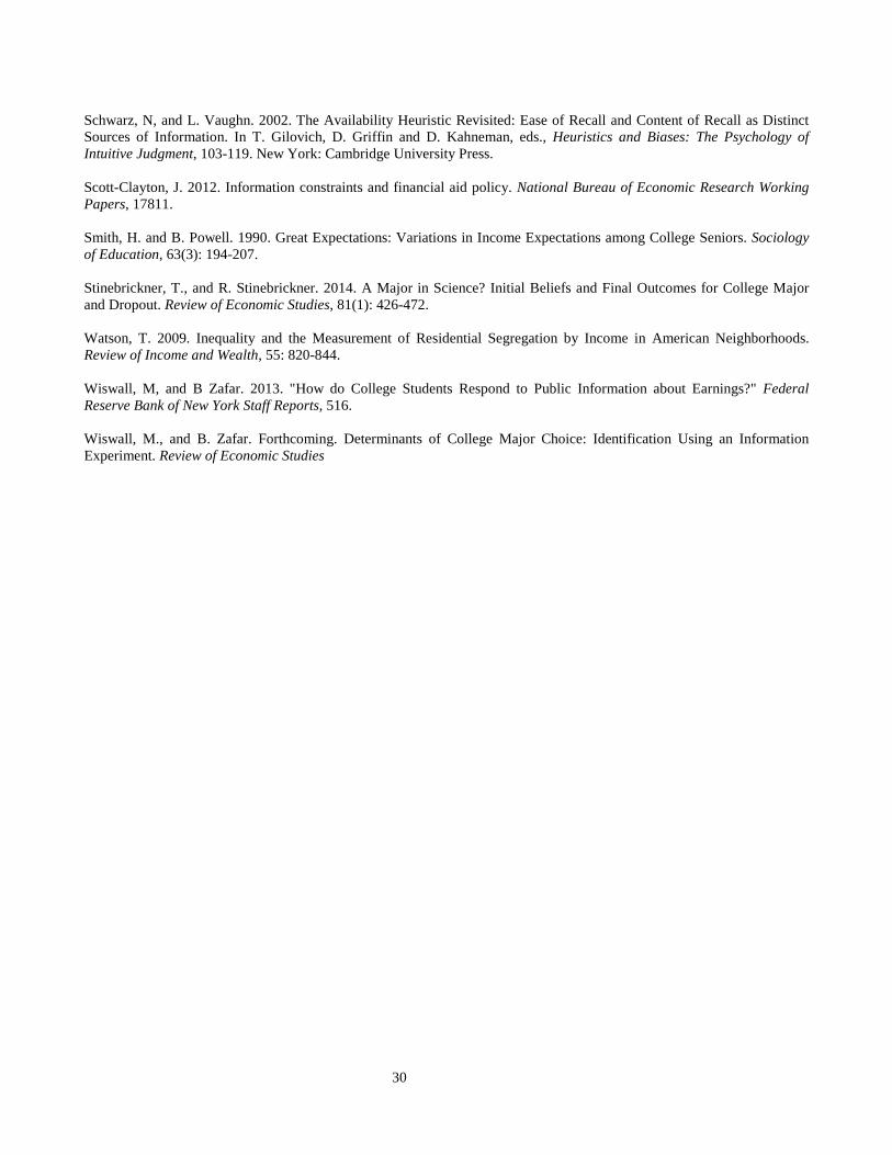
30

Schwarz, N, and L. Vaughn. 2002. The Availability Heuristic Revisited: Ease of Recall and Content of Recall as Distinct Sources of Information. In T. Gilovich, D. Griffin and D. Kahneman, eds., Heuristics and Biases: The Psychology of Intuitive Judgment, 103-119. New York: Cambridge University Press. Scott-Clayton, J. 2012. Information constraints and financial aid policy. National Bureau of Economic Research Working Papers, 17811. Smith, H. and B. Powell. 1990. Great Expectations: Variations in Income Expectations among College Seniors. Sociology of Education, 63(3): 194-207. Stinebrickner, T., and R. Stinebrickner. 2014. A Major in Science? Initial Beliefs and Final Outcomes for College Major and Dropout. Review of Economic Studies, 81(1): 426-472. Watson, T. 2009. Inequality and the Measurement of Residential Segregation by Income in American Neighborhoods. Review of Income and Wealth, 55: 820-844. Wiswall, M, and B Zafar. 2013. "How do College Students Respond to Public Information about Earnings?" Federal Reserve Bank of New York Staff Reports, 516. Wiswall, M., and B. Zafar. Forthcoming. Determinants of College Major Choice: Identification Using an Information Experiment. Review of Economic Studies

31

7. APPENDIX In this section, we discuss the implications of the elasticity estimates (reported in Table 7) on non-college

respondents’ college attendance decisions. Because we are asking respondents for their prospective college costs

many years after they made their own college attendance decisions (of not to attend college), it is likely that

their responses systematically differ from the beliefs that they held prior to making their decision, say, due to ex

post rationalization. For example, individuals who decided to not attend college may overestimate their

prospective costs in order to justify their decision. Moreover, we do not know the actual college cost these

individuals would have faced had they chosen to attend college.

Nevertheless, our data allows us to provide a first-pass answer to this question, proxying individuals’

overestimation of their own college cost with their current overestimation of the population average public

sticker cost.34 This implicitly assumes that the current error in respondents’ perceived college costs is a good

proxy for their stock of knowledge regarding college costs at the time of the respondent’s decision of not

attending college. This is a strong assumption, justified only in part by the strong correlation between population

beliefs and self own beliefs regarding college costs shown in column (7) of Table 4, but it is helpful in

understanding the magnitude and importance of our estimated elasticities. The results of this experiment are

presented in column (4) of Table 7. We find that our calculated elasticities imply an average increase in the

likelihood of college attendance of 34.5%, although the standard deviation is very high, suggesting substantial

heterogeneity. The likelihood of college attendance rises more for higher-income individuals than lower-income

individuals, though the differences is not statistically significant, and even lower-income individuals’ likelihood

of college attendance rises by about 30%. This finding is very similar in magnitude to that of Dynarski (2003),

who quasi-experimentally finds that eligibility for student benefits (which decrease college costs) increases

college attendance by 22.4% on average within her lower-income sample.

34 We use perceived public university costs in our experiment, and conservatively compare them to the average public sticker costs from the College Board. Results are qualitatively similar using public net costs, or comparing perceived population private costs to private net costs.

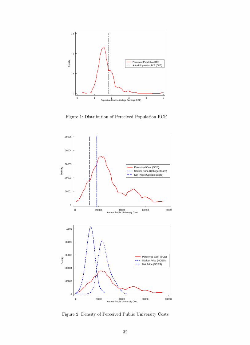
0

.5

1

1.5

Den

sity

0 1 2 3 4 5Population Relative College Earnings (RCE)

Perceived Population RCEActual Population RCE (CPS)

Figure 1: Distribution of Perceived Population RCE

0

.00001

.00002

.00003

.00004

.00005

Den

sity

0 20000 40000 60000 80000Annual Public University Cost

Perceived Cost (SCE)Sticker Price (College Board)Net Price (College Board)

0

.00002

.00004

.00006

.00008

.0001

Den

sity

0 20000 40000 60000 80000Annual Public University Cost

Perceived Cost (SCE)Sticker Price (NCES)Net Price (NCES)

Figure 2: Density of Perceived Public University Costs

32

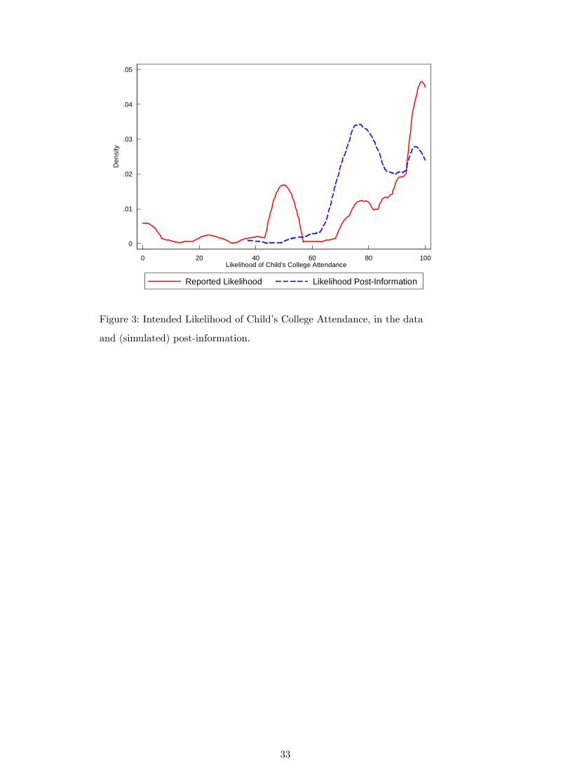
0

.01

.02

.03

.04

.05

Den

sity

0 20 40 60 80 100Likelihood of Child's College Attendance

Reported Likelihood Likelihood Post­Information

Figure 3: Intended Likelihood of Child’s College Attendance, in the data

and (simulated) post-information.

33

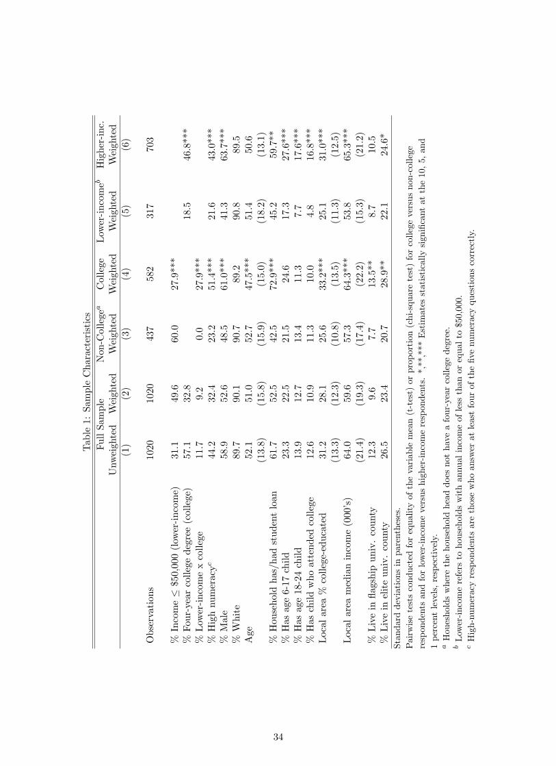
Table1:SampleCharacteristics

FullSample

Non-Collegea

College

Lower-incomeb

Higher-inc.

Unweighted

Weighted

Weighted

Weighted

Weighted

Weighted

(1)

(2)

(3)

(4)

(5)

(6)

Observations

1020

1020

437

582

317

703

%Income≤$50,000(lower-income)

31.1

49.6

60.0

27.9***

%Four-yearcollegedegree(college)

57.1

32.8

18.5

46.8***

%Lower-incomexcollege

11.7

9.2

0.0

27.9***

%Highnumeracyc

44.2

32.4

23.2

51.4***

21.6

43.0***

%Male

58.9

52.6

48.5

61.0***

41.3

63.7***

%White

89.7

90.1

90.7

89.2

90.8

89.5

Age

52.1

51.0

52.7

47.5***

51.4

50.6

(13.8)

(15.8)

(15.9)

(15.0)

(18.2)

(13.1)

%Householdhas/hadstudentloan

61.7

52.5

42.5

72.9***

45.2

59.7**

%Hasage6-17child

23.3

22.5

21.5

24.6

17.3

27.6***

%Hasage18-24child

13.9

12.7

13.4

11.3

7.7

17.6***

%Haschildwhoattendedcollege

12.6

10.9

11.3

10.0

4.8

16.8***

Localarea%college-educated

31.2

28.1

25.6

33.2***

25.1

31.0***

(13.3)

(12.3)

(10.8)

(13.5)

(11.3)

(12.5)

Localareamedianincome(000’s)

64.0

59.6

57.3

64.3***

53.8

65.3***

(21.4)

(19.3)

(17.4)

(22.2)

(15.3)

(21.2)

%Liveinflagshipuniv.county

12.3

9.6

7.7

13.5**

8.7

10.5

%Liveineliteuniv.county

26.5

23.4

20.7

28.9**

22.1

24.6*

Standarddeviationsinparentheses.

Pairwisetestsconductedforequalityofthevariablemean(t-test)orproportion(chi-squaretest)forcollegeversusnon-college

respondentsandforlower-incomeversushigher-incomerespondents.*,**,***Estimatesstatisticallysignificantatthe10,5,and

1percentlevels,respectively.

aHouesholdswherethehouseholdheaddoesnothaveafour-yearcollegedegree.

bLower-incomereferstohouseholdswithannualincomeoflessthanorequalto$50,000.

cHigh-numeracyrespondentsarethosewhoansweratleastfourofthefivenumeracyquestionscorrectly.

34

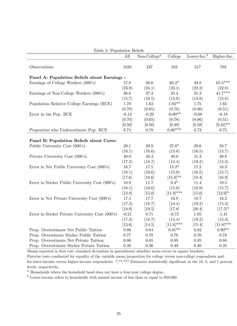
Table 2: Population BeliefsAll Non-Collegea College Lower-Inc.b Higher-Inc.

Observations 1020 437 582 317 703

Panel A: Population Beliefs about Earnings :Earnings of College Workers (000’s) 57.8 56.6 60.2* 49.8 65.5***

(23.9) (24.1) (23.1) (22.2) (22.8)Earnings of Non-College Workers (000’s) 36.6 37.2 35.4 31.3 41.7***

(15.7) (16.5) (13.9) (13.8) (15.8)Population Relative College Earnings (RCE) 1.70 1.63 1.83** 1.75 1.65

(0.70) (0.65) (0.78) (0.86) (0.51)Error in the Pop. RCE -0.13 -0.20 -0.00** -0.08 -0.18

(0.70) (0.65) (0.78) (0.86) (0.51)[0.50] [0.50] [0.49] [0.58] [0.42]**

Proportion who Underestimate Pop. RCE 0.74 0.78 0.66*** 0.73 0.75

Panel B: Population Beliefs about Costs:Public University Cost (000’s) 29.1 29.9 27.6* 29.6 28.7

(16.1) (16.6) (15.0) (16.5) (15.7)Private University Cost (000’s) 40.0 40.3 40.0 41.3 38.8

(17.3) (18.7) (14.4) (19.2) (15.3)Error in Net Public University Cost (000’s) 16.7 17.5 15.2* 17.2 16.3

(16.1) (16.6) (15.0) (16.5) (15.7)[17.6] [18.6] [15.8]** [18.4] [16.9]

Error in Sticker Public University Cost (000’s) 10.9 11.7 9.4* 11.4 10.5(16.1) (16.6) (15.0) (16.9) (15.7)[13.9] [15.0] [11.9]*** [15.0] [12.9]*

Error in Net Private University Cost (000’s) 17.4 17.7 16.9 18.7 16.2(17.3) (18.7) (14.4) (19.2) (15.3)[18.9] [19.5] [17.8] [20.4] [17.5]*

Error in Sticker Private University Cost (000’s) -0.21 0.71 -0.72 1.05 -1.41(17.3) (18.7) (14.4) (19.2) (15.3)[13.6] [14.5] [11.6]*** [15.4] [11.8]***

Prop. Overestimate Net Public Tuition 0.86 0.84 0.91** 0.82 0.90**Prop. Overstimate Sticker Public Tuition 0.77 0.78 0.76 0.76 0.78Prop. Overestimate Net Private Tuition 0.86 0.85 0.89 0.85 0.88Prop. Overestimate Sticker Private Tuition 0.38 0.36 0.40 0.40 0.35Means reported in first row; standard deviations in parentheses; absolute mean errors in square brackets.Pairwise tests conducted for equality of the variable mean/proportion for college versus non-college respondents andfor lower-income versus higher-income respondents. *,**,*** Estimates statistically significant at the 10, 5, and 1 percentlevels, respectively.a Households where the household head does not have a four-year college degree.b Lower-income refers to households with annual income of less than or equal to $50,000.

35

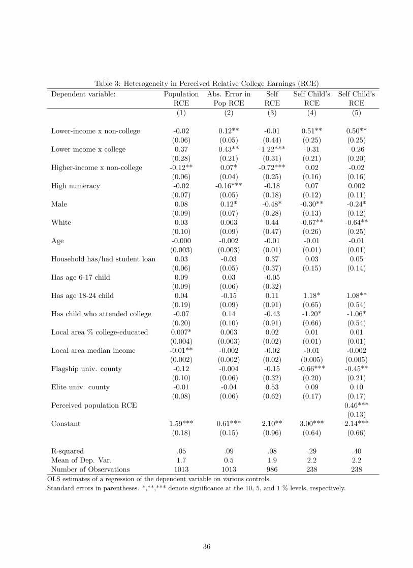
Table 3: Heterogeneity in Perceived Relative College Earnings (RCE)Dependent variable: Population Abs. Error in Self Self Child’s Self Child’s

RCE Pop RCE RCE RCE RCE(1) (2) (3) (4) (5)

Lower-income x non-college -0.02 0.12** -0.01 0.51** 0.50**(0.06) (0.05) (0.44) (0.25) (0.25)

Lower-income x college 0.37 0.43** -1.22*** -0.31 -0.26(0.28) (0.21) (0.31) (0.21) (0.20)

Higher-income x non-college -0.12** 0.07* -0.72*** 0.02 -0.02(0.06) (0.04) (0.25) (0.16) (0.16)

High numeracy -0.02 -0.16*** -0.18 0.07 0.002(0.07) (0.05) (0.18) (0.12) (0.11)

Male 0.08 0.12* -0.48* -0.30** -0.24*(0.09) (0.07) (0.28) (0.13) (0.12)

White 0.03 0.003 0.44 -0.67** -0.64**(0.10) (0.09) (0.47) (0.26) (0.25)

Age -0.000 -0.002 -0.01 -0.01 -0.01(0.003) (0.003) (0.01) (0.01) (0.01)

Household has/had student loan 0.03 -0.03 0.37 0.03 0.05(0.06) (0.05) (0.37) (0.15) (0.14)

Has age 6-17 child 0.09 0.03 -0.05(0.09) (0.06) (0.32)

Has age 18-24 child 0.04 -0.15 0.11 1.18* 1.08**(0.19) (0.09) (0.91) (0.65) (0.54)

Has child who attended college -0.07 0.14 -0.43 -1.20* -1.06*(0.20) (0.10) (0.91) (0.66) (0.54)

Local area % college-educated 0.007* 0.003 0.02 0.01 0.01(0.004) (0.003) (0.02) (0.01) (0.01)

Local area median income -0.01** -0.002 -0.02 -0.01 -0.002(0.002) (0.002) (0.02) (0.005) (0.005)

Flagship univ. county -0.12 -0.004 -0.15 -0.66*** -0.45**(0.10) (0.06) (0.32) (0.20) (0.21)

Elite univ. county -0.01 -0.04 0.53 0.09 0.10(0.08) (0.06) (0.62) (0.17) (0.17)

Perceived population RCE 0.46***(0.13)

Constant 1.59*** 0.61*** 2.10** 3.00*** 2.14***(0.18) (0.15) (0.96) (0.64) (0.66)

R-squared .05 .09 .08 .29 .40Mean of Dep. Var. 1.7 0.5 1.9 2.2 2.2Number of Observations 1013 1013 986 238 238OLS estimates of a regression of the dependent variable on various controls.Standard errors in parentheses. *,**,*** denote significance at the 10, 5, and 1 % levels, respectively.

36

Table4:HeterogeneityinPerceivedCollegeCosts

Dependentvariable:

Pop.Public

Abs.ErrorinPub.Cost

Pop.Private

Abs.ErrorinPriv.Cost

SelfCollege

Univ.Cost

(NetPrice)

(StickerPrice)

Univ.Cost

(NetPrice)

(StickerPrice)

Cost

(1)

(2)

(3)

(4)

(5)

(6)

(7)

Lower-incomexnon-college

0.99

1.34

2.05

1.27

2.18

3.52***

8.79***

(1.89)

(1.77)

(1.54)

(2.19)

(2.02)

(1.27)

(1.77)

Lower-incomexcollege

-2.56

-2.02

-1.13

-2.21

-1.29

2.78**

-1.36

(2.02)

(1.87)

(1.60)

(2.82)

(2.58)

(1.31)

(2.06)

Higher-incomexnon-college

-0.25

-0.04

0.46

-3.28**

-2.43*

0.64

14.3***

(1.61)

(1.48)

(1.34)

(1.58)

(1.37)

(1.03)

(1.62)

Highnumeracy

-1.16

-1.33

-0.86

-2.07

-2.3*

-1.73**

-5.25***

(1.46)

(1.38)

(1.18)

(1.45)

(1.30)

(0.86)

(1.25)

Male

-2.64

-2.19

-1.64

-2.43

-1.66

0.08

-0.84

(1.63)

(1.51)

(1.30)

(1.78)

(1.62)

(1.05)

(1.56)

White

1.51

0.76

.05

-2.01

-3.18

-2.36*

0.99

(2.22)

(1.95)

(1.69)

(2.98)

(2.48)

(1.33)

(1.9)

Age

0.42

0.38

0.20

0.40

0.42

0.27

-1.25***

(0.31)

(0.29)

(0.24)

(0.38)

(0.34)

(0.22)

(0.36)

Agesquared

-0.004

-0.003

-0.002

-0.004

-0.004

-0.003

0.01***

(0.003)

(0.003)

(0.003)

(0.004)

(0.003)

(0.002)

(0.003)

Householdhas/hadstudentloan

-0.16

-0.57

-0.77

-0.53

-0.69

-0.77

-0.57

(1.51)

(1.38)

(1.21)

(1.76)

(1.56)

(1.00)

(1.54)

Hasage6-17child

0.96

1.66

2.35*

1.5

2.38

2.34*

-1.01

(1.84)

(1.66)

(1.42)

(2.38)

(2.14)

(1.30)

(1.87)

Hasage18-24child

12.2***

11.1**

10.1**

17.5*

15.6*

11.2*

-1.56

(4.53)

(4.43)

(4.12)

(8.95)

(8.75)

(5.97)

(4.94)

Haschildwhoattendedcollege

-13.0***

-12.4***

-11.0**

-17.8*

-16.5*

-13.0**

4.33

(4.84)

(4.74)

(4.38)

(9.27)

(9.05)

(5.97)

(5.49)

Localarea%college-educated

-0.06

-0.08

-0.08

0.05

0.03

-0.12**

-0.05

(0.09)

(0.09)

(0.08)

(.08)

(.07)

(.05)

(.08)

Localareamedianincome

0.03

0.03

0.01

0.02

0.01

0.02

0.01

(0.05)

(0.05)

(0.04)

(0.05)

(0.05)

(0.03)

(0.05)

Flagshipuniv.county

-2.47

-2.44

-2.29

-2.26

-1.67

0.10

-0.13

(1.91)

(1.77)

(1.57)

(1.92)

(1.60)

(1.34)

(1.75)

Eliteuniv.county

0.16

-0.32

-0.32

-2.26

-3.06**

-1.74*

1.45

(1.71)

(1.66)

(1.46)

(1.62)

(1.49)

(0.89)

(1.45)

Perceivedpop.publicuniv.cost

0.30***

(0.05)

Perceivedpop.privateuniv.cost

0.09**

(0.05)

Constant

19.1**

9.33

10.5*

29.8***

9.77

12.4**

55.6***

(8.06)

(7.37)

(6.39)

(10.6)

(9.58)

(5.38)

(9.64)

R-squared

.04

.05

.05

.06

.07

.12

.30

MeanofDep.Var.

2918

1440

1914

24NumberofObservations

1020

1020

1020

1019

1019

1019

1013

Thedependentvariableisin’000sofdollars.

OLSestimatesofaregressionofthedependentvariableonvariouscontrols.

Standarderrorsinparentheses.*,**,***denotesignificanceatthe10,5,and1%levels,respectively.

37

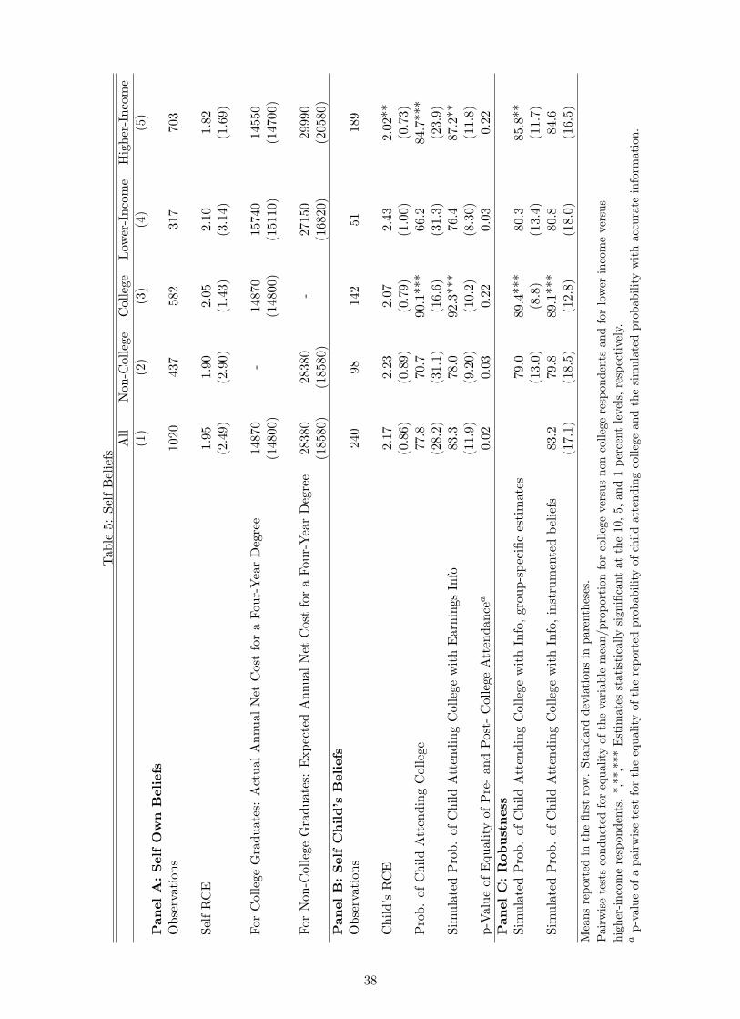
Table5:SelfBeliefsAll

Non-College

College

Lower-Income

Higher-Income

(1)

(2)

(3)

(4)

(5)

PanelA:SelfOwnBeliefs

Observations

1020

437

582

317

703

SelfRCE

1.95

1.90

2.05

2.10

1.82

(2.49)

(2.90)

(1.43)

(3.14)

(1.69)

ForCollegeGraduates:ActualAnnualNetCostforaFour-YearDegree

14870

-14870

15740

14550

(14800)

(14800)

(15110)

(14700)

ForNon-CollegeGraduates:ExpectedAnnualNetCostforaFour-YearDegree

28380

28380

-27150

29990

(18580)

(18580)

(16820)

(20580)

PanelB:SelfChild’sBeliefs

Observations

240

98142

51189

Child’sRCE

2.17

2.23

2.07

2.43

2.02**

(0.86)

(0.89)

(0.79)

(1.00)

(0.73)

Prob.ofChildAttendingCollege

77.8

70.7

90.1***

66.2

84.7***

(28.2)

(31.1)

(16.6)

(31.3)

(23.9)

SimulatedProb.ofChildAttendingCollegewithEarningsInfo

83.3

78.0

92.3***

76.4

87.2**

(11.9)

(9.20)

(10.2)

(8.30)

(11.8)

p-ValueofEqualityofPre-andPost-CollegeAttendancea

0.02

0.03

0.22

0.03

0.22

PanelC:Robustness

SimulatedProb.ofChildAttendingCollegewithInfo,group-specificestimates

79.0

89.4***

80.3

85.8**

(13.0)

(8.8)

(13.4)

(11.7)

SimulatedProb.ofChildAttendingCollegewithInfo,instrumentedbeliefs

83.2

79.8

89.1***

80.8

84.6

(17.1)

(18.5)

(12.8)

(18.0)

(16.5)

Meansreportedinthefirstrow.Standarddeviationsinparentheses.

Pairwisetestsconductedforequalityofthevariablemean/proportionforcollegeversusnon-collegerespondentsandforlower-incomeversus

higher-incomerespondents.*,**,***Estimatesstatisticallysignificantatthe10,5,and1percentlevels,respectively.

ap-valueofapairwisetestfortheequalityofthereportedprobabilityofchildattendingcollegeandthesimulatedprobabilitywithaccurateinformation.

38

Table 6: Determinant’s of the College Decision of the ChildDependent variable: Probability of attending college by child age:

6-17 6-17 6-17 6-24(1) (2) (3) (4)

Lower-income x non-college -28.2*** -20.4* -19.1* -9.04(5.73) (11.1) (11.5) (8.90)

Lower-income x college -21.9** -17.4 -16.7 -13.1(9.04) (12.6) (12.9) (10.6)

Higher-income x non-college -15.7*** -17.0*** -17.2*** -6.81*(4.31) (4.44) (4.39) (3.47)

High numeracy 1.46 -0.79 -1.28 1.12(3.95) (4.00) (4.03) (3.48)

Male 0.62 -0.16 -0.13 -1.78(5.00) (4.41) (4.37) (3.812)

White -4.35 -12.33*** -12.74*** -12.25***(4.12) (4.74) (4.83) (4.42)

Age -0.30 -0.23 -0.24 -0.04(0.29) (0.27) (0.28) (0.27)

Household has/had student loan 3.61 -1.36 -1.29(4.97) (4.31) (4.22)

Has age 18-24 child -19.012 -13.44 -13.03(20.67) (13.42) (13.53)

Has child who attended college 22.02 13.72 13.45(20.89) (13.64) (13.71)

Local area % college-educated -0.01 0.24 0.21 0.48*(0.30) (0.29) (0.29) (0.25)

Local area median income -0.07 -0.15 -0.13 -0.21(0.17) (0.16) (0.16) (0.13)

Flagship univ. county 5.10 0.98 1.65 -3.76(8.00) (6.82) (7.11) (6.867)

Elite univ. county 3.74 4.16 4.12 2.72(5.17) (4.72) (4.79) (3.54)

Child’s RCE 53.0*** 51.8*** 49.4***(13.1) (13.0) (13.9)

Child’s RCE squared -9.69*** -9.64*** -9.44***(2.32) (2.31) (2.59)

Perceived public university cost 0.29* 0.28* 0.14(0.15) (0.15) (0.13)

Perc. pub. univ. cost x lower-income -0.20 -0.23 -0.43*(0.27) (0.28) (0.25)

Population RCE 3.11(3.79)

Constant 94.0*** 29.1 26.5 37.1*(13.2) (20.2) (20.8) (20.6)

R-squared .23 .33 .33 .30Mean of Dep. Var. 78 78 78 81Number of Observations 240 238 238 378OLS estimates of a regression of the child’s college attendance likelihood (on a 0-100 scale)on various controls.Standard errors in parentheses. *,**,*** denote significance at 10, 5, and 1 %, respectively.

39

Table7:SensitivityofSelfCollegeEnrollmenttoChangesinCollegeCosts

Num.of

∆CollegeAttendance

Elasticity

∆College

Obs.

Prob.if

Likelihood

(1)

(2)

(3)

(4)

PanelA:Non-CollegeRespondents

Costs−20%a

Cost−50%

All

417

22.2

36.5

-1.93

34.5

(27.1)

(34.7)

(3.91)

(42.1)

[198/57]b

Lower-Income

188

21.1

35.6

-2.07

30.4

(27.0)

(35.1)

(4.11)

(41.3)

[85/31]

Higher-Income

229

23.8

37.8

-1.75

37.9

(23.5)

(34.2)

(3.63)

(42.5)

[113/26]

PanelB:College-EducatedRespondents

Costs

+20%

Costs

+40%

All

568

87.1

81.6

-0.60

(23.4)

(27.1)

(1.01)

[288/18]

Lower-Income

112

83.9

77.6

-0.77

(27.6)

(32.5)

(1.24)

[50/6]

Higher-Income

456

88.3

83.1

-0.54

(21.7)

(24.8)

(0.90)

[238/12]

Meansreportedinfirstrow.Standarddeviationsinparentheses.

aChangeincollegeattendanceprobabilityifcollegecostsdecreasedby20%.

b[a/b]aisthenumberofrespondentswithelasticity0(insensitivetocostchange),andbis

thenumberofrespondentswhoseelasticitiescouldnotbecomputed.

40

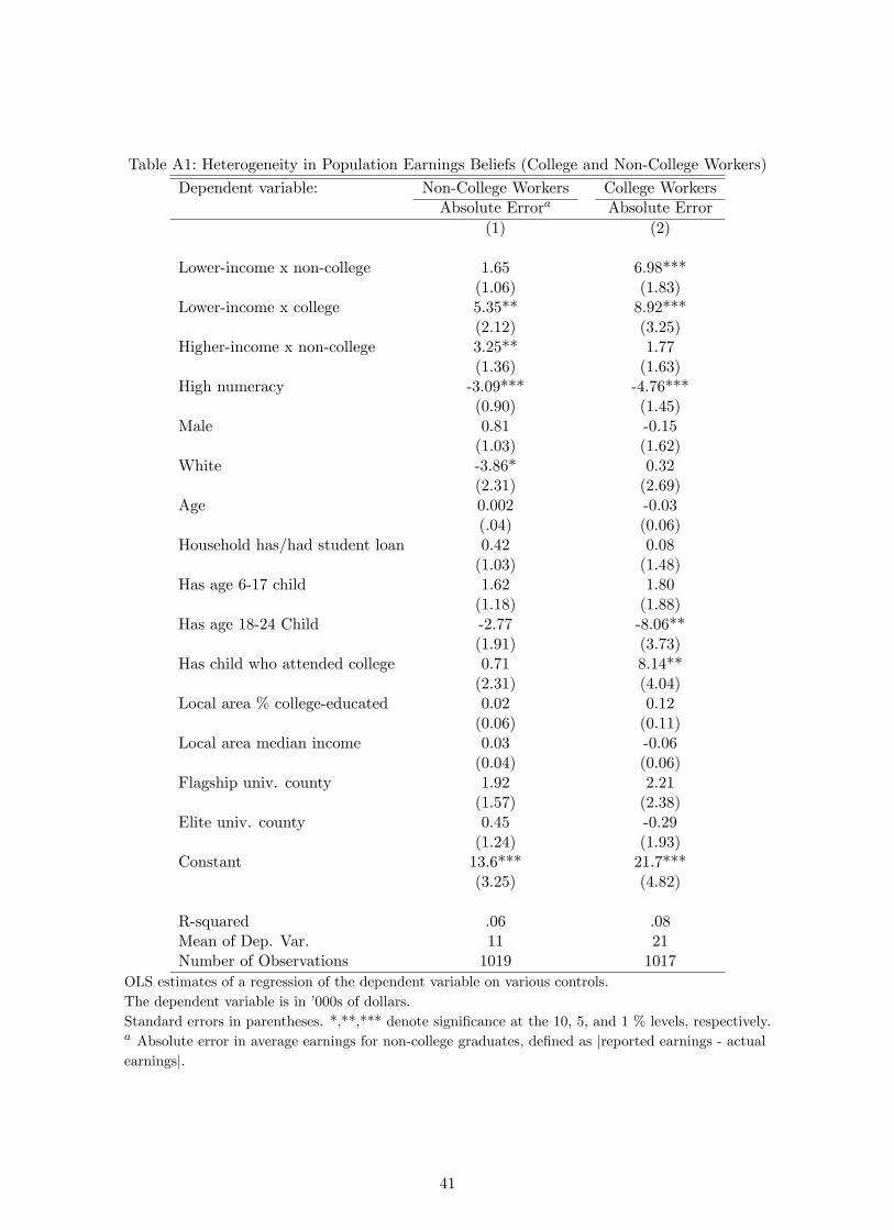
Table A1: Heterogeneity in Population Earnings Beliefs (College and Non-College Workers)

Dependent variable: Non-College Workers College WorkersAbsolute Errora Absolute Error

(1) (2)

Lower-income x non-college 1.65 6.98***(1.06) (1.83)

Lower-income x college 5.35** 8.92***(2.12) (3.25)

Higher-income x non-college 3.25** 1.77(1.36) (1.63)

High numeracy -3.09*** -4.76***(0.90) (1.45)

Male 0.81 -0.15(1.03) (1.62)

White -3.86* 0.32(2.31) (2.69)

Age 0.002 -0.03(.04) (0.06)

Household has/had student loan 0.42 0.08(1.03) (1.48)

Has age 6-17 child 1.62 1.80(1.18) (1.88)

Has age 18-24 Child -2.77 -8.06**(1.91) (3.73)

Has child who attended college 0.71 8.14**(2.31) (4.04)

Local area % college-educated 0.02 0.12(0.06) (0.11)

Local area median income 0.03 -0.06(0.04) (0.06)

Flagship univ. county 1.92 2.21(1.57) (2.38)

Elite univ. county 0.45 -0.29(1.24) (1.93)

Constant 13.6*** 21.7***(3.25) (4.82)

R-squared .06 .08Mean of Dep. Var. 11 21Number of Observations 1019 1017

OLS estimates of a regression of the dependent variable on various controls.The dependent variable is in ’000s of dollars.Standard errors in parentheses. *,**,*** denote significance at the 10, 5, and 1 % levels, respectively.a Absolute error in average earnings for non-college graduates, defined as |reported earnings - actualearnings|.

41

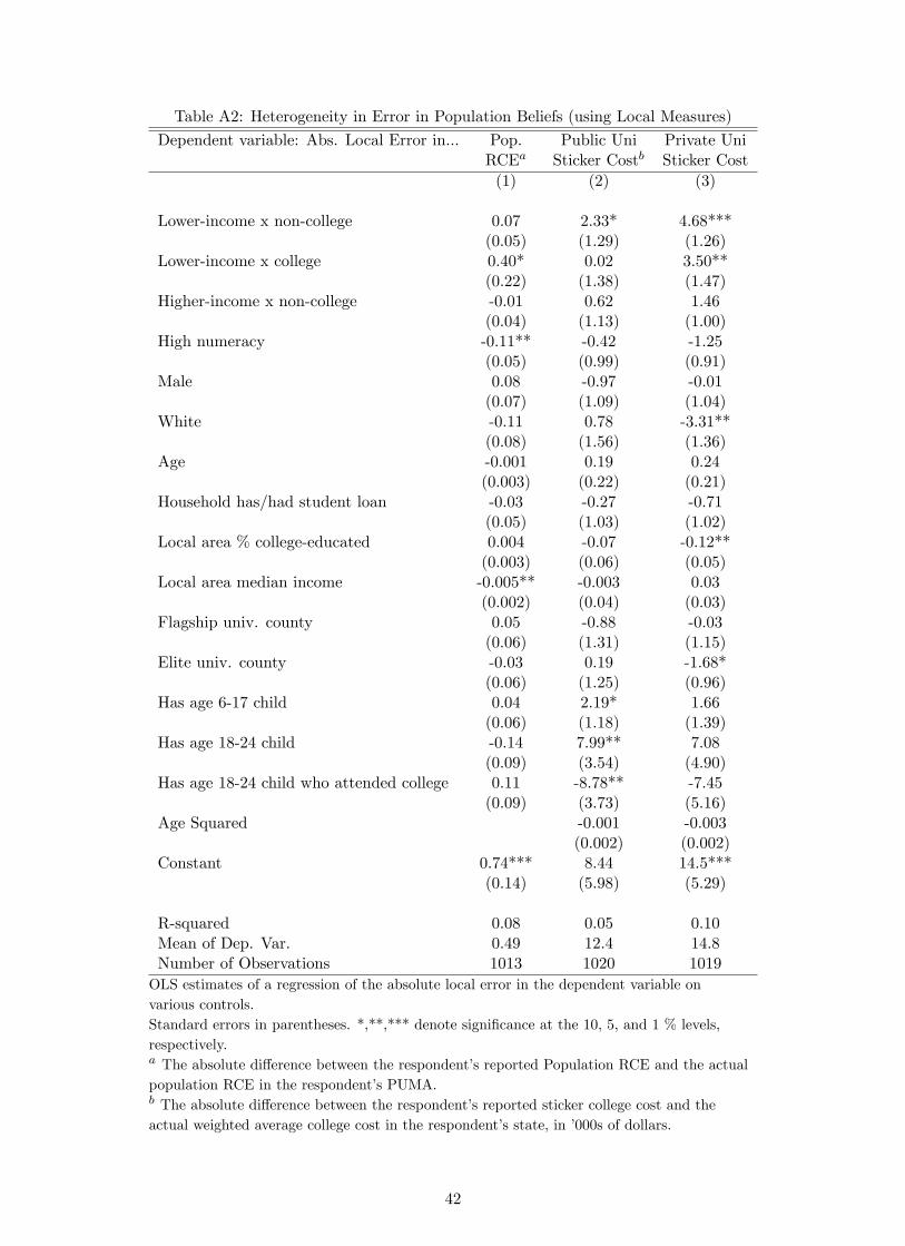
Table A2: Heterogeneity in Error in Population Beliefs (using Local Measures)

Dependent variable: Abs. Local Error in... Pop. Public Uni Private UniRCEa Sticker Costb Sticker Cost(1) (2) (3)

Lower-income x non-college 0.07 2.33* 4.68***(0.05) (1.29) (1.26)

Lower-income x college 0.40* 0.02 3.50**(0.22) (1.38) (1.47)

Higher-income x non-college -0.01 0.62 1.46(0.04) (1.13) (1.00)

High numeracy -0.11** -0.42 -1.25(0.05) (0.99) (0.91)

Male 0.08 -0.97 -0.01(0.07) (1.09) (1.04)

White -0.11 0.78 -3.31**(0.08) (1.56) (1.36)

Age -0.001 0.19 0.24(0.003) (0.22) (0.21)

Household has/had student loan -0.03 -0.27 -0.71(0.05) (1.03) (1.02)

Local area % college-educated 0.004 -0.07 -0.12**(0.003) (0.06) (0.05)

Local area median income -0.005** -0.003 0.03(0.002) (0.04) (0.03)

Flagship univ. county 0.05 -0.88 -0.03(0.06) (1.31) (1.15)

Elite univ. county -0.03 0.19 -1.68*(0.06) (1.25) (0.96)

Has age 6-17 child 0.04 2.19* 1.66(0.06) (1.18) (1.39)

Has age 18-24 child -0.14 7.99** 7.08(0.09) (3.54) (4.90)

Has age 18-24 child who attended college 0.11 -8.78** -7.45(0.09) (3.73) (5.16)

Age Squared -0.001 -0.003(0.002) (0.002)

Constant 0.74*** 8.44 14.5***(0.14) (5.98) (5.29)

R-squared 0.08 0.05 0.10Mean of Dep. Var. 0.49 12.4 14.8Number of Observations 1013 1020 1019OLS estimates of a regression of the absolute local error in the dependent variable onvarious controls.Standard errors in parentheses. *,**,*** denote significance at the 10, 5, and 1 % levels,respectively.a The absolute difference between the respondent’s reported Population RCE and the actualpopulation RCE in the respondent’s PUMA.b The absolute difference between the respondent’s reported sticker college cost and theactual weighted average college cost in the respondent’s state, in ’000s of dollars.

42