Embed Size (px)
Citation preview

ESCUELA DE INGENIERIAS INDUSTRIALES
DEPARTAMENTO DE INGENIERIA DE SISTEMAS Y AUTOMATICA
TESIS DOCTORAL:
ROBUST STABILIZATION AND OBSERVATION FOR POSITIVE TAKAGI-SUGENO SYSTEMS
Presentada por Ines Zaidi para optar al grado de doctora por la Universidad de Valladolid
Dirigida por: Dr. Fernando Tadeo
Dr. Mohamed Chaabane

To my great parents M ohamed and Zouhour. To my grandfather Hbib and my aunt Kalthoum.
To my sister Asma and brother Anis. To all those who offered me their help and support,
in my ongoing journey, to reach what I have being dreaming of,
and to become who I want to be.
1

Acknowledgement
I strongly believe that everything happens for a reason. Looking back at my life, I can see clearly the major events and circumstances which I have encountered along my way and which have had an influence on my life progress, even it was bad or good. Obviously, I have learnt to exploit the consequences of these events in my favor and neglect the effects of those which were against my destination. While struggling to achieve what I am meant to do, nothing has been more valuable to me than the support and assistance of those ones who have not hesitated to provide me with love, compassion, kindness and even a big sense of responsibility. I am really grateful for their help and for making the level of my self-confidence as high as possible during my PhD work. That is why, at the beginning of my dissertation, I have the honor to acknowledge these precious persons who made my PhD time one of the greatest steps in my whole life.
First and foremost, my sincere gratitude goes to my direct supervisor Dr. Fernando Tadeo for hosting me in the laboratory of Systems Engineering and Automatic Control of Valladolid University and for his patience, availability, and ongoing support. Added to that, the fact that he is one of the nicest people I have ever known made my Ph.D. life much more fruitful than I expected. I will always be indebted to him for everything he has done for me.
I also wish to express my appreciation and gratitude to my thesis director in Sfax University: Dr. Mohamed Chaabane, Professor at Sfax University and the director of the Unity of Sciences and Techniques of Automatic Control and Computer Engineering (Lab-STA), for his confidence, charisma and good advice over the dissertation years. I thank him for his trust, support, innovative ideas he has given me, the growing interest shown in my work, his encouragement and his availability during this time.
I must confess that it was an honor for me to work with people of such excellent skills and reputations, both nationally and internationally without forgetting to mention their human qualities and good humor that made each encounter a pleasant moment.
2

My stay at the Department of Systems Engineering and Automatic Control of Valladolid University has been an exciting adventure in the aim of the knowledge and understanding of the world around us. This presents for me a great experience at both scientific and human levels.
I am very grateful for the honor that made me Dr. Ahmed El Hajjaji, Professor at the University of Picardie Jules Vernes (France), Dr. Driss Mehdi, Professor at the University of Poitiers (France) and Dr. Fouad Mesquine, Professor at the Physics Department of Cadi Ayyad University (Marrakech), accepting the task of evaluating the work presented in this thesis. Their valuable and helpful comments were for me a great help to improve the quality of my dissertation.
I especially thank Dr. Abdellah Benzaouia, professor at the University of Cadi Ayyad (Marrakech) where he is also head of the laboratory of research LAEPT, CNRST laboratory for collaborating with us, for inviting me to his laboratory in the aim of establishing common works, for his fructuous ideas and ongoing guidance in my dissertation study.
I have many good memories from my times at Valladolid University; a brilliant research environment with many first-class researchers. I thank all my current and former colleagues who provided such a superb research environment. I like to thank all of them for their sincere friendships, for all the good times and interesting conversations we had, inside or outside the university.
I address my special thanks to the staff of the department od Systems Engineering and Automatic Control, particularly Teresa de Jesús and Graciano, for always being nice and helpful. I cannot finish describing how much I appreciate their efforts in resolving my technical problems and their availability at each time I needed them.
Finally, I wish to express my gratitude to the Creator, infinite source of inspiration and to my family for their daily support, encouragement and great availability. From smallest to largest, you have been strength of my mind and an example of loyal love to accomplish my dissertation.
Keep your trust in me, I will make you proud..
3

I.Z.
4

“M easure what is measurable and make measurable what is not so”. Galileo Galilei.
“The sacred formula of positivists: Love as principle, Order as basis and Progress as end”.
August Comte. “They did not know it was impossible so they did it”
M arc Twain.
5

6

Summary
List of Figures .................................................................................................... 13
Notations ............................................................................................................ 16
Introduction ....................................................................................................... 21
0.1. Introduction .................................................................................................... 23
0.2. Overview ........................................................................................................ 25
0.3. Publications .................................................................................................... 27
Chapter I ............................................................................................................ 31
State of the Art ................................................................................................. 31
Background ........................................................................................................... 33
1.1. State of the Art of Takagi-Sugeno (T-S) systems .......................................... 33
1.1.1. Takagi-Sugeno models ............................................................................. 33
1.1.2. Stability and Stabilization of Takagi-Sugeno systems ............................. 34
1.1.2.1. The direct Lyapunov approach ......................................................... 34
1.1.2.2. Stability of Takagi-Sugeno systems .................................................. 37
1.1.2.3. Stabilization of Takagi-Sugeno systems ............................................ 37
1.1.3. Observer Design for Takagi-Sugeno systems ........................................... 39
1.1.3.1. Measurable decision variables (MDV)............................................... 40
1.1.3.2. Unmeasurable decision variables (UDV) ........................................... 41
1.1.4. Observer-Based Control for Takagi-Sugeno systems ............................... 42
1.1.4.1. Measurable decision variables (MDV)............................................... 42
1.1.4.2. Unmeasurable decision variables (UDV) ........................................... 44
1.2. State of the Art of time-delay Takagi-Sugeno systems .................................. 44
1.2.1. Time-delay systems .................................................................................. 44
1.2.2. Classification of delay models .................................................................. 44
1.2.2.2. Plus variable delay ............................................................................ 45
1.2.2.3. Bounded variable delay ..................................................................... 45
7

1.2.2.4. Variable delay with constraint on the derivative .............................. 45
1.2.2.5. Variable delay with bounded derivative ........................................... 46
1.2.3. Classification of time-delay Takagi-Sugeno models ................................. 46
1.2.3.1. Takagi-Sugeno model with delayed state .......................................... 46
1.2.3.2. Takagi-Sugeno model with delayed control ...................................... 47
1.2.3.3. Takagi-Sugeno model with delayed state and control....................... 47
1.2.4. Stabilization by PDC control of T-S systems with time-delay ................ 48
1.2.5. Relaxation techniques .............................................................................. 49
1.3. State of the Art of Positive Systems .............................................................. 51
1.3.1. Introduction ............................................................................................. 51
1.3.2. Definition and properties of Positive Systems ......................................... 51
1.3.2.1. Notations and Definitions ................................................................. 51
1.3.2.2. Properties of Metzler Matrices .......................................................... 52
1.3.2.3. Properties of Positive Systems .......................................................... 54
1.3.2.4. Positive Linear Systems .................................................................... 55
1.3.2.5. Stability of Positive Linear Systems ................................................. 56
1.3.3. Positive Linear Systems with time-delay ................................................. 57
1.3.3.1. Stability Analysis .............................................................................. 58
1.3.3.2. PDC Controller Design ..................................................................... 61
1.3.4. Positive Takagi-Sugeno systems .............................................................. 62
1.3.5. Review on positive time-delay Takagi-Sugeno Systems .......................... 64
1.4. Conclusion ...................................................................................................... 65
Chapter II ........................................................................................................... 69
Stability and Stabilization of Positive Takagi-Sugeno systems .............. 69
2.1. Introduction .................................................................................................... 71
2.2. Stability and Stabilization of Positive Takagi-Sugeno systems with measurable premise variables ................................................................................ 71
2.2.1. Positive Stabilization by memoryless state-feedback ............................... 72
2.2.2.1. Positive Asymptotic Stabilization ..................................................... 72
8

2.2.2.2. Positive Exponential Stabilization .................................................... 75
2.2.2.3. Relaxed Positive Exponential Stabilization Conditions .................... 76
2.2.3. Positive Stabilization of Nonpositive Takagi-Sugeno systems ................. 78
2.2.3.1. Positive Asymptotic Stabilization of T-S systems ............................ 79
2.2.3.2. Illustrative Examples......................................................................... 82
2.2.4. Stabilization by Memory state-feedback .................................................. 85
2.2.5. Robust Interval 𝛼𝛼-stabilization of Positive T-S systems with memory state-feedback .................................................................................................... 87
2.2.6. Positive Stabilization by output-feedback controller ............................... 88
2.2.6.1. Output-feedback Stabilization for Positive Takagi-Sugeno systems . 89
2.2.6.2. Illustrative Example .......................................................................... 92
2.3. Stability and Stabilization of Positive Takagi-Sugeno Systems with unmeasurable premise variables ............................................................................ 93
2.3.1. Stability and Stabilization by memoryless state-feedback controller ...... 94
2.3.1.1. Approach using the description of the state estimation error with disturbance .................................................................................................... 95
2.3.1.2. Approach assuming bounded inputs and states .............................. 100
2.3.1.3. Illustrative Example ........................................................................ 105
2.4. Conclusion .................................................................................................... 108
Chapter III ....................................................................................................... 111
Observer-Based Control Design for Positive Systems ............................ 111
3.1. Introduction .................................................................................................. 113
3.2. Observation of Linear Positive Systems ....................................................... 113
3.2.1. Interval observers approach ................................................................... 113
3.2.1.1. Interval observer design using upper and lower errors.................... 113
3.2.1.2. Design of Positive Observers for Interval Systems .......................... 117
3.2.1.3. Design of Positive Interval Observer-based state-feedback controller ..................................................................................................................... 118
3.2.1.4. Illustrative example ......................................................................... 123
9

3.3. Observer-based Control Design for Positive T-S Systems ........................... 124
3.3.1. Observer-based control of Positive T-S systems with measurable premise variables........................................................................................................... 125
3.3.1.1. Positive T-S observer-based controller (First approach) ................ 125
3.3.1.2. Positive Interval Observer for Autonomous Positive T-S systems . 129
3.3.1.3. Positive Interval T-S Observer-based Controller (Second approach) ..................................................................................................................... 132
3.3.2. Observer design of Positive T-S systems with unmeasurable premise variables........................................................................................................... 134
3.3.2.1. Positive 𝐿𝐿2 observer design for positive T-S systems ...................... 135
3.3.2.2. Illustrative examples ....................................................................... 139
3.3.2.3. Positive Interval Observer-Based Controller design for Positive T-S systems with unmeasurable premise variables ............................................. 147
3.3.2.4. Illustrative example: Two-tanks Hydraulic System ........................ 153
3.4. Conclusion ................................................................................................. 157
Chapter IV ....................................................................................................... 159
Stability and Stabilization of Positive time-delay systems .................... 159
4.1. Introduction .................................................................................................. 161
4.1.1. Asymptotic Stability of Positive Linear time-delay systems ................. 162
4.1.1.1. Case of a single constant delay ....................................................... 162
4.1.1.2. Case of variable and multiple delays ............................................... 165
4.1.2. Stabilization of Positive Linear time-delay systems .............................. 169
4.1.2.1. State-feedback Stabilization of Positive Linear time-delay systems 169
4.1.2.2. Stabilization of Positive Linear time-delay systems with a decomposed memory state-feedback control ................................................ 173
4.2. Stabilization of Positive Takagi-Sugeno systems with time-delay .............. 177
4.2.1. Introductory remarks ............................................................................. 177
4.2.2. Stabilization of Positive T-S time-delay systems with a decomposed state-feedback control ............................................................................................... 177
10

4.2.2.1. Asymptotic Stabilization of Positive T-S systems with time-delay with decomposed state-feedback controller.................................................. 177
4.2.2.2. Robust 𝛼𝛼-stabilization of positive T-S systems with time-delay with decomposed state-feedback controller .......................................................... 179
4.2.2.3. Illustrative Example: Hydraulic two-tank-system ........................... 183
4.2.2.4. Asymptotic Stabilization of Positive time-delay T-S systems with decomposed memory state-feedback controller ............................................ 188
4.2.2.5. Illustrative Example ........................................................................ 192
4.3. Conclusion .................................................................................................... 194
Chapter V ......................................................................................................... 195
Observers and Controllers for Positive systems with time-delay ........ 195
5.1. Introduction .................................................................................................. 197
5.2. Positive Observer design for Positive Linear systems with time-delay ........ 197
5.2.1. Positive Observer design for Positive Autonomous Linear systems with time-delay ........................................................................................................ 197
5.2.2. Positive Observer design for Positive Interval Linear systems with time-delay ................................................................................................................ 201
5.2.3. Illustrative Example .............................................................................. 205
5.3. Positive Observer-Based Controller design for Positive Interval Linear systems with time-delay ...................................................................................... 207
5.3.1. Theoretical approach ............................................................................. 207
5.3.2. Illustrative Example .............................................................................. 212
5.4. Positive Observer-Based Controller design for Positive Interval T-S systems with time-delay ................................................................................................... 215
5.4.1. Case 1: Measurable premise variables .................................................... 215
5.4.2. Case 2: Unmeasurable premise variables ............................................... 221
5.4.3. Illustrative Example: Hydraulic two-tank system ................................. 228
5.5. Conclusion .................................................................................................... 234
Conclusions and Perspectives ....................................................................... 237
6.1. Summary and Contributions ........................................................................ 239
11

6.2. Future Lines of Research.............................................................................. 240
Annex: Important Lemmas ........................................................................... 241
Bibliography ..................................................................................................... 243
Objetivos, metodología y resultados generales del trabajo .................... 271
12

List of Figures
Figure 2. 1. The evolution of the states 𝑥𝑥1, 𝑥𝑥2 and 𝑥𝑥3 for the closed-loop system 83
Figure 2. 2. The evolution of the states 𝑥𝑥1 and 𝑥𝑥2 for the closed-loop system ..... 85
Figure 2. 3. Stabilization of the system (2.79) via OPDC control (2.70) ............. 93
Figure 2. 4. Principle of the state observer ........................................................... 95
Figure 2. 5. The evolution of the system input 𝑢𝑢(𝑡𝑡) ........................................... 106
Figure 2. 6. The evolution of the state estimation error 𝑒𝑒1(𝑡𝑡) ............................ 107
Figure 2. 7. The evolution of the state estimation error 𝑒𝑒2(𝑡𝑡) ............................ 107
Figure 2. 8. The evolution of the state estimation error 𝑒𝑒3(𝑡𝑡) ............................ 108
Figure 3. 1. Evolution of the state 𝑥𝑥1(𝑡𝑡) and its estimation 𝑥𝑥�1(𝑡𝑡) ..................... 123
Figure 3. 2. Evolution of the state 𝑥𝑥2(𝑡𝑡) and its estimation 𝑥𝑥�2(𝑡𝑡) ..................... 124
Figure 3. 3. Evolution of the estimation errors 𝑒𝑒1(𝑡𝑡) and 𝑒𝑒2(𝑡𝑡) ......................... 124
Figure 3. 4. Evolution of the Lyapunov function 𝑉𝑉(𝑥𝑥(𝑡𝑡)) in (3.157) .................. 141
Figure 3. 5. Evolution of the state 𝑥𝑥1(𝑡𝑡) and its estimation 𝑥𝑥�1(𝑡𝑡) ..................... 141
Figure 3. 6. Evolution of the state 𝑥𝑥2(𝑡𝑡) and its estimation 𝑥𝑥�2(𝑡𝑡) ..................... 142
Figure 3. 7. Evolution of the state 𝑥𝑥3(𝑡𝑡) and its estimation 𝑥𝑥�3(𝑡𝑡) ..................... 142
Figure 3. 8. Evolution of the estimation error 𝑒𝑒1(𝑡𝑡) ........................................... 142
Figure 3. 9. Evolution of the estimation error 𝑒𝑒2(𝑡𝑡) ........................................... 143
Figure 3. 10. Evolution of the estimation error 𝑒𝑒3(𝑡𝑡) ......................................... 143
Figure 3. 11. Electrical Circuit (Kaczorek, 2012) ................................................ 143
Figure 3. 12. Evolution of the voltage sources 𝑣𝑣1 and 𝑣𝑣2 ................................... 145
Figure 3. 13. The evolution of the current 𝑖𝑖1(𝑡𝑡) ................................................. 146
Figure 3. 14. The evolution of the current 𝑖𝑖2(𝑡𝑡) ................................................. 146
Figure 3. 15. The evolution of the current 𝑖𝑖3(𝑡𝑡) ................................................. 147
Figure 3. 16. Structure of the two-tank hydraulic system (Zhang & Ding, 2005) ............................................................................................................................ 154
Figure 3. 17. The evolution of the pump flows ................................................... 156
Figure 3. 18. Evolution of the state 𝑥𝑥1(𝑡𝑡) and its estimation 𝑥𝑥�1(𝑡𝑡) .................... 157
Figure 3. 19. Evolution of the state 𝑥𝑥2(𝑡𝑡) and its estimation 𝑥𝑥�2(𝑡𝑡).................... 157
Figure 4. 1. State trajectories of 𝑥𝑥1(𝑡𝑡), ∀𝑡𝑡 ∈ [−9,0] ........................................... 187
13

Figure 4. 2. State trajectories of 𝑥𝑥2(𝑡𝑡), ∀𝑡𝑡 ∈ [−9,0] ........................................... 187
Figure 4. 3. The evolution of the two pump flows 𝑢𝑢1(𝑡𝑡) and 𝑢𝑢2(𝑡𝑡) .................... 188
Figure 4. 4. State trajectory of 𝑥𝑥1(𝑡𝑡) .................................................................. 193
Figure 4. 5. State trajectory of 𝑥𝑥2(𝑡𝑡) .................................................................. 194
Figure 4. 6. Evolution of the system inputs 𝑢𝑢1(𝑡𝑡) and 𝑢𝑢2(𝑡𝑡) .............................. 194
Figure 5. 1. Two-compartment model with the definition of model parameters 205
Figure 5. 2.The evolution of the interval estimates of 𝑥𝑥1(𝑡𝑡) ............................... 206
Figure 5. 3.The evolution of the interval estimates of 𝑥𝑥2(𝑡𝑡) ............................... 206
Figure 5. 4. Evolution of the state 𝑥𝑥1(𝑡𝑡), and its estimation for 𝑥𝑥0 = [5 4]𝑇𝑇 ..... 214
Figure 5. 5. Evolution of the state 𝑥𝑥2(𝑡𝑡) and its estimation for 𝑥𝑥0 = [5 4]𝑇𝑇 ...... 214
Figure 5. 6. Evolution of the estimation errors 𝑒𝑒1(𝑡𝑡) and 𝑒𝑒2(𝑡𝑡) ......................... 215
Figure 5. 7. Evolution of the two pump flows 𝑢𝑢1(𝑡𝑡) and 𝑢𝑢2(𝑡𝑡) ........................... 233
Figure 5. 8. Evolution of the state 𝑥𝑥1(𝑡𝑡) and its estimation ............................... 233
Figure 5. 9. Evolution of the state 𝑥𝑥2(𝑡𝑡) and its estimation ............................... 234
14

15

Notations
• Matrices and Vectors
𝐼𝐼 identity matrix of appropriate dimensions
𝐼𝐼𝑛𝑛×𝑛𝑛 𝑛𝑛 × 𝑛𝑛 Identity matrix
0𝑝𝑝×𝑞𝑞 𝑝𝑝 × 𝑞𝑞 matrix with all entries equal to 0.
0 Matrix of appropriate dimensions with all entries equal to 0.
𝑃𝑃 > 0 (𝑃𝑃 ≥ 0)
Square and positive definite matrix (resp. positive semi-definite)
𝑃𝑃 < 0 (𝑃𝑃 ≤ 0)
Square and negative definite matrix (resp. semi-negative definite)
𝑋𝑋 > 𝑌𝑌 (𝑋𝑋 ≥ 𝑌𝑌) The matrix 𝑋𝑋 − 𝑌𝑌 is positive definite (resp. semi-positive definite)
𝑑𝑑𝑖𝑖𝑑𝑑𝑑𝑑(𝑑𝑑) Diagonal matrix with diagonal components the elements of 𝑑𝑑
𝑃𝑃𝑇𝑇 Transpose of 𝑃𝑃
𝑃𝑃−1 Inverse of 𝑃𝑃
𝑃𝑃−𝑇𝑇 Shorthand for (𝑃𝑃−1)𝑇𝑇
𝜆𝜆(𝑃𝑃) Eigenvalue of 𝑃𝑃
𝜆𝜆𝑚𝑚𝑚𝑚𝑛𝑛(𝑃𝑃) Minimum eigenvalue of 𝑃𝑃
𝜆𝜆𝑚𝑚𝑚𝑚𝑚𝑚(𝑃𝑃) Maximum eigenvalue of 𝑃𝑃
�𝑃𝑃11 𝑃𝑃12∗ 𝑃𝑃22
� Symmetric matrix with (∗) representing 𝑃𝑃12𝑇𝑇
𝑅𝑅𝑒𝑒(𝑃𝑃) Real part of the eigenvalues of the matrix 𝑃𝑃
𝐼𝐼𝐼𝐼(𝑃𝑃) Imaginary part of the eigenvalues of the matrix 𝑃𝑃
|𝑑𝑑| Absolute value of 𝑑𝑑
16

‖𝑋𝑋‖ Norm 2 of the vector 𝑋𝑋: �|𝑥𝑥1|2 + ⋯ + |𝑥𝑥𝑛𝑛|2
𝐻𝐻2 Norm 2 of a system
𝐻𝐻∞ Norm ∞ of a system
∆𝐴𝐴 Additive uncertainty on the matrix 𝐴𝐴
[𝐴𝐴]𝑚𝑚𝑖𝑖 Element located at the 𝑖𝑖th row and 𝑗𝑗th column of matrix A
𝐴𝐴 ≽ 0 Nonnegative matrix: ∀(𝑖𝑖, 𝑗𝑗), [𝐴𝐴]𝑚𝑚𝑖𝑖 ≥ 0
𝐴𝐴 ≻ 0 Positive matrix: ∀(𝑖𝑖, 𝑗𝑗), [𝐴𝐴]𝑚𝑚𝑖𝑖 > 0
𝐴𝐴 ≽ 𝐵𝐵 The matrix 𝐴𝐴 − 𝐵𝐵 ≽ 0
𝐴𝐴 ∈ [𝐴𝐴, 𝐴𝐴] 𝐴𝐴 ≼ 𝐴𝐴 ≼ �̅�𝐴
∀ For all
∈ Belongs to
𝜇𝜇(𝐴𝐴) The spectral abscissa of the matrix 𝐴𝐴 (max of the real parts of the eigenvalues of 𝐴𝐴)
→ Tends toward
⇒ Implies
∎ End of the proof
� ℎ𝑚𝑚ℎ𝑖𝑖ℎ𝑘𝑘
𝑟𝑟
𝑚𝑚,𝑖𝑖,𝑘𝑘=1
� � � ℎ𝑚𝑚ℎ𝑖𝑖ℎ𝑘𝑘
𝑟𝑟
𝑘𝑘=1
𝑟𝑟
𝑖𝑖=1
𝑟𝑟
𝑚𝑚=1
�̇�𝑋(𝑡𝑡) The derivative of the vector 𝑋𝑋 with respect of time
𝑋𝑋�(𝑡𝑡) The estimation of the vector 𝑋𝑋
Metzler 𝐴𝐴 All its off-diagonal elements are nonnegative, i.e., ∀(𝑖𝑖, 𝑗𝑗), 𝑖𝑖 ≠𝑗𝑗, [𝐴𝐴]𝑚𝑚𝑖𝑖 ≥ 0
17

• Sets and Areas
ℝ Set of real numbers
ℝ𝑛𝑛×𝑛𝑛 Space of matrices with real entries
ℝ+ Set of positive or null real numbers
ℝ+∗ Set of positive real numbers
ℝ+𝑛𝑛×𝑛𝑛 Positive orthant of ℝ𝑛𝑛×𝑛𝑛
𝐶𝐶1 Set of the continuously differentiable functions
• Acronyms
LMI Linear Matrix Inequality
BMI Bilinear Matrix Inequality
LP Linear Programming
LTI Linear Time Invariant
LTV Linear Time Variant
PDC Parallel Distributed Control
PPDC Proportional Parallel Distributed Control
OPDC Output Parallel Distributed Control
CDF Compensation and Division by Fuzzy model
GEVP General Eigenvalue Problem
T-S Takagi-Sugeno
MDV Measurable Decision Variables
UDV Unmeasurable Decision Variables
18

• Notations of Multimodels
𝑥𝑥(𝑡𝑡) The state of the system: 𝑥𝑥(𝑡𝑡) ∈ ℝ𝑛𝑛𝑥𝑥
𝑢𝑢(𝑡𝑡) The input of the system: 𝑢𝑢(𝑡𝑡) ∈ ℝ𝑛𝑛𝑢𝑢
𝑦𝑦(𝑡𝑡) The output of the system: 𝑦𝑦(𝑡𝑡) ∈ ℝ𝑛𝑛𝑦𝑦
𝐴𝐴𝑚𝑚 The state matrix of the 𝑖𝑖th LTI submodel: 𝐴𝐴𝑚𝑚 ∈ ℝ𝑛𝑛𝑥𝑥×𝑛𝑛𝑥𝑥
𝐵𝐵𝑚𝑚 The input matrix of the 𝑖𝑖th LTI submodel: 𝐵𝐵𝑚𝑚 ∈ ℝ𝑛𝑛𝑥𝑥×𝑛𝑛𝑢𝑢
𝐶𝐶𝑚𝑚 The output matrix of the 𝑖𝑖th LTI submodel: 𝐶𝐶𝑚𝑚 ∈ ℝ𝑛𝑛𝑦𝑦×𝑛𝑛𝑥𝑥
19

Introduction Ines Zaidi
20

Introduction Ines Zaidi
Introduction
21

Introduction Ines Zaidi
22

Introduction Ines Zaidi
In this chapter, we discuss the motivation behind this thesis and provide an overview of the material presented in the manuscript.
0.1. Introduction
The assumption of linearity in practical systems makes possible to develop simple models that approximate its behavior. These linear models have been extensively studied in different contexts: identification, state estimation, control, diagnosis, etc. However, such models allow the representation of the behavior of a system only around a given operating point, as the linearity assumption is verified only in a restricted area of the operating space. Given that real systems are not linear in nature, the performance of control and diagnosis systems based on linear models degrade when moving away from the operating point. In order to improve the system performance, it is imperative to take into account the nonlinearities in the modeling phase. This allows describing the behavior of a real system over a wide operating range with better accuracy than with linear models. Control and diagnostic systems developed using nonlinear models are then more efficient than those developed from linear models. The main drawback of nonlinear models is the complexity of their mathematical structures, which makes them difficult to use. For this reason, studies on nonlinear systems do not have a general framework, but relate to specific classes of nonlinear models, such as Lipchitz systems, bilinear systems, Takagi-Sugeno (T-S) systems, LPV systems, etc. In this dissertation, we concentrate on T-S systems, as the tools used resemble those of linear systems.
In many investigations on dynamical systems, the state vector is assumed to be available for measurement. However, such an assumption is not always true in practice, as for technical and/or economic reasons, it is not possible to measure all state variables. However, the need to know fully the state variables of the system is often crucial, which requires the use of tools to estimate variables which are not accessible to measurement. This makes the problem of observer design a fundamental issue in control systems.
The first works on the problem of state reconstruction were dedicated to linear systems (Luenberger, 1971). Many theoretical results were then proposed and are widely used in control and estimation. For example, the diagnostic of operating systems is based on linear models (Gertler, 1998), (Patton et al, 1989), (Isermann, 2007), (Ding, 2008). However, the linearity of the model is a strong assumption
23

Introduction Ines Zaidi
which limits the validity of the results obtained. Furthermore, a direct extension of the methods developed for linear models to nonlinear models is tricky. Many techniques have been then dedicated to state estimation of particular classes of nonlinear systems (based on changes in a canonical form of observability, Kalman filter, observer, Luenberger extended observers...) (Kalman, 1960), (Chen & Patton, 1999). However, these techniques are often difficult to apply because of the imposed constraints. In addition, the wealth of results for linear systems is very little exploitable in the context of nonlinear systems.
The strategy of state reconstruction proposed in this thesis uses a technique to obtain a model, taking into account the nonlinearities of the system and providing a simple and exploitable mathematical structure. This is generally called a multimodel approach. Several types of multimodels have been introduced in recent years, such as multimodels with coupled states and multimodels with single states, called Takagi-Sugeno (T-S) models (Tanaka & Wang, 2001), (Orjuela, 2008).
T-S models are the most studied in the literature: they are described by a set of submodels sharing a single state vector (Takagi & Sugeno, 1985). Two categories can be considered depending on the nature of the variables involved in the weighting functions. Indeed, these variables, called decision variables or premise variables, can be known (input, output of the system, etc.) or unknown (system state, etc.). The category of T-S models with measurable decision variables (VDM) has been the subject of many developments in control, stabilization, state estimation (Tanaka & Wang, 2001) and diagnosis (Nagy et al, 2009).
A new constraint is currently been added in the synthesis of control and estimation systems, on the sign of the variables. Positive systems are those whose states remain nonnegative for all future times, once started from nonnegative initial conditions. Positivity is not an inherent property of a system; we might be able to turn a nonpositive system into a positive system with a simple change of variable (Zaidi et al, 2012). Such systems can be found in practice in different areas of science and technology, such as: biology and physiology where biochemical models have a common important characteristic which is that most variables take only nonnegative values, since they usually represent chemical concentrations (Sontag, 2005), (Vahid, 2012), (Haddad & Chellaboina, 2005), in Communications, mainly in congestion control in TCP networks (Shorten et al, 2006), (Jacquez & Simon, 1993), Economics (Leontief, 1936), (Neumann, 1945),
24

Introduction Ines Zaidi
Compartmental systems (Benvenuti & Farina, 2002), Ecology and population dynamics (Lotka, 1925), (Volterra, 1926), etc.
Even though stability properties of positive linear time-invariant systems are now well investigated (Bolajraf, 2012), (Benzaouia et al, 2011), (Benzaouia & El Hajjaji, 2011), (Benzaouia et al, 2014), (Rami & Tadeo, 2008), (Rami & Tadeo, 2007a), (Rami & Tadeo, 2007b) there are still a lot of unanswered questions in other classes of positive systems, such as uncertain nonlinear systems, or time-delay systems. Although there is a rich literature on properties of uncertain systems, they have been rarely studied in the context of nonlinear positive systems. To deal with this deficiency, in this thesis, we deal with stabilization and 𝛼𝛼-stabilization of nonlinear systems, especially positive Takagi-Sugeno and time-delay systems. We also present conditions for stability and stabilization of positive time-delay systems, when the size of delay is fixed or variable. We also applied static memoryless state-feedback control laws, with and without memory, in order to guarantee a performing stabilization for such systems.
0.2. Overview
We begin by setting the context and providing the state of the art for much of the later work in Chapter 1. We define various concepts and results that will be used in the following sections. Firstly, we will have an overview on the Takagi-Sugeno (T-S) modeling approach and the stabilization and estimation of this type of systems. Secondly, a background is deserved to the classification and modeling of time-delay T-S systems. Then, we focus on the stability and stabilization of time-delay T-S systems. Later on, the design of observers and observer-based controllers will be introduced, concentrating on positive systems and their properties. Then, we focus on positivity of linear systems and their properties. Classes of time-delay T-S systems, which will be repeatedly used in the following chapters, are discussed in the context of guaranteeing their stability and positivity. 𝛼𝛼-stability will be discussed thoroughly in the different chapters of the thesis; therefore, we discuss in this chapter basic stability properties.
In Chapter 2, we are interested in the analysis of stability and stabilization of positive nonlinear systems described by T-S models that only involve nonnegative states. Firstly, we introduce the concept of asymptotic stability and 𝛼𝛼-stability of positive T-S systems, where the main stability and stabilization approaches depend on the type of the premise variables: measurable or unmeasurable.
25

Introduction Ines Zaidi
Moreover, we are interested in robust stabilization and robust 𝛼𝛼-stabilization of positive T-S systems with interval uncertainties. Memory state-feedback controllers for positive interval systems have been then established.
In Chapter 3, firstly, LMI conditions are established in order to synthesize interval observers for positive linear systems, that can provide lower and upper estimates on the unmeasurable states. This can be done by minimizing an adequate bound on the interval errors and can be solved via an LMI optimization problem. Secondly, we establish approaches for the design of positive observer-based controllers for positive T-S systems with measurable and unmeasurable premise variables, with and without interval uncertainties. Numerical and practical examples are presented to show the effectiveness of the proposed methods.
Chapter 4 is dedicated to the study of positive time-delay systems, with and without interval uncertainties. Firstly, we introduce stability results with constant and multiple delays. Secondly, we will deal with the asymptotic stabilization and the robust 𝛼𝛼-stabilization. Finally, necessary and sufficient conditions are provided for the asymptotic stabilization and robust 𝛼𝛼-stabilization of positive interval T-S time-delay systems by means of state-feedback laws with or without memory. We also consider the decomposition of the state-feedback controller gains in order to reduce the conservatism.
Chapter 5 is firstly devoted to the design of positive observers for positive linear time-delay systems, with and without interval uncertainties: necessary and sufficient conditions have been established and expressed in terms of LMIs, taking into account the positivity constraints. Secondly, observer-based controllers have been synthesized for positive linear time-delay systems to guarantee the stability and positivity of the closed-loop system. Necessary conditions are formulated in order to check the existence of any solutions to the problem of continuous-time observer-based control. Once satisfied, we study the sufficient conditions and the corresponding synthesis for this problem. Moreover, extensions of these approaches are applied for positive interval Takagi-Sugeno systems with variable time-delay. In this issue, we consider when the decision variables are measurable and when they are not.
Finally, illustrative results of numerical and practical examples have been given to show the effectiveness of these approaches.
26

Introduction Ines Zaidi
In the Conclusion, we summarize the results and outlining possible directions for extending those results.
0.3. Publications
Journal papers
1. Zaidi, I., Chaabane, M., Tadeo, F., & Benzaouia, A. (2015). Static state-feedback controller and observer design for interval positive systems with time-delay. IEEE Transactions on Circuits and Systems II, Accepted in December 2014.
2. Zaidi, I., Chaabane, M., Tadeo, F., & Benzaouia, A. (2015). Robust 𝛼𝛼-stabilization of uncertain positive T-S systems via memory state-feedback. Circuits, Systems and Signal Processing (CSSP), Submitted in October 2014.
3. Zaidi, I., Chaabane, M., Tadeo, F., & Benzaouia, A. (2015). Stabilization of positive Takagi-Sugeno systems by a decomposed memory state-feedback controller. Nonlinear analysis: Hybrid Systems, Submitted in October 2014.
Conference papers
1. Zaidi, I., Tadeo, F., Chaabane, M., & Benzaouia, A. (2012a). Positive observation of Takagi-Sugeno Systems. In the 17th International Conference on Methods and Models in Automation and Robotics (MMAR), Miedzyzdrojie, Poland.
2. Zaidi, I., & Tadeo, F. (2012b). Control of Continuous-time Takagi-Sugeno Systems for Stability and Positivity. In the 17th International Conference on Methods and Models in Automation and Robotics (MMAR), Miedzyzdrojie, Poland.
3. Zaidi, I., Tadeo, F., & Chaabane, M. (2012c). Stability and Positive State Estimation for Takagi-Sugeno Systems”. In the 14th Sciences and Techniques of Automatic Conference (STA), Sousse, Tunisia.
4. Zaidi, I., Tadeo, F., & Chaabane, M. (2013a). Positive Observer Based Tracking Controller Design for Takagi-Sugeno Systems”. In the 10th
27

Introduction Ines Zaidi
Conference on Systems, Signals and Devices Conference (SSD), Hammamet, Tunisia.
5. Zaidi, I., Tadeo, F., & Chaabane, M. (2013b). Positive State Estimation with 𝐻𝐻∞ performance for Positive Continuous-time Takagi Sugeno Systems. In European Student paper Competition (ESPC-ISA) Conference, Lisboa, Portugal.
6. Zaidi, I., Tadeo, F., & Chaabane, M. (2013c). Positive observer design for continuous-time Takagi-Sugeno systems. In Proc. of the 52nd Decision and Control Conference (CDC), 5030-5035, Florence, Italy.
7. Zaidi, I., Tadeo, F., & Chaabane, M. (2014a). Positive Observers for Continuous time Positive Interval Systems with time-delay. In the 15th Sciences and Techniques of Automatic Conference (STA), Sousse, Tunisia.
8. Zaidi, I., Tadeo, F., & Chaabane, M. (2014b). Design of Robust Observers for Positive Delayed Interval Systems. In the 11th Conference on Systems, Signals and Devices Conference (SSD), Barcelona, Spain.
9. Zaidi, I., Tadeo, F., & Chaabane, M. (2015). Stabilization of positive Takagi-Sugeno systems with unmeasurable premise variables. In the 4th International Conference on Systems and Control (ICSC), Accepted.
Communications
1. Zaidi, I. (2014). Robust stabilization and observation of positive Takagi-Sugeno systems. XII Simposio CEA de Ingeniería de Control "Ingeniería de Control: de la Teoría a la Práctica", Universidad de Valladolid, Spain: 6-7 de Febrero.
2. Workshop on "Intelligent Planning and Control: Bringing together adaptive control and reinforcement learning for guaranteeing Optimal Performance and Robustness”. In Proc. of the 52nd Decision and Control Conference (CDC), 5030-5035, Florence, Italy.
28

Introduction Ines Zaidi
29

I. State of the Art Ines Zaidi
30

I. State of the Art Ines Zaidi
Chapter I
State of the Art
31

I. State of the Art Ines Zaidi
32

I. State of the Art Ines Zaidi
Background
This chapter provides the mathematical basis required for the results presented in the following chapters. More precisely, we recall some basic definitions and results related to dynamical systems.
1.1. State of the Art of Takagi-Sugeno (T-S) systems
Firstly, we provide an overview on the Takagi-Sugeno (T-S) modeling approach, concentrating on the stabilization and estimation of this type of systems. Secondly, the modeling of time-delay T-S systems is discussed. Then, we focus on the stability, stabilization of time-delay T-S systems, followed by the design of observers and observer-based controllers. At the end of this chapter, we focus on the positivity of linear and T-S systems and their properties, including time-delay positive systems, which will be repeatedly used in the following chapters.
1.1.1. TAKAGI-SUGENO MODELS
Recently, many investigations have revealed the importance of Takagi-Sugeno systems in modern system control, as it can be considered as a nonlinear combination of a set of linear systems interconnected by nonlinear weighting functions (Tanaka et al, 2001), (Ichalal , 2009). This type of modeling is very useful thanks to its ability of approximating different complex systems, and then applying simple control and estimation approaches to get remarkable results.
The representation of nonlinear systems introduced as T-S models (Takagi & Sugeno, 1985) is an interesting alternative in the field of control, observation and diagnosis. Specifically, a Takagi-Sugeno system is described by fuzzy IF-THEN rules, which locally represent linear input-output relations called subsystems. Each of these rules is of the following form:
Rule 𝑖𝑖: IF 𝑧𝑧1(𝑡𝑡) is 𝐹𝐹𝑚𝑚1 and …and 𝑧𝑧𝑝𝑝(𝑡𝑡) is 𝐹𝐹𝑚𝑚
𝑝𝑝 THEN:
�̇�𝑥(𝑡𝑡) = 𝐴𝐴𝑚𝑚𝑥𝑥(𝑡𝑡) + 𝐵𝐵𝑚𝑚𝑢𝑢(𝑡𝑡) (1.1)
𝑦𝑦(𝑡𝑡) = 𝐶𝐶𝑚𝑚𝑥𝑥(𝑡𝑡) + 𝐷𝐷𝑚𝑚𝑢𝑢(𝑡𝑡) (1.2)
where 𝑥𝑥(𝑡𝑡) ∈ ℝ𝑛𝑛𝑥𝑥 is the state vector , 𝑢𝑢(𝑡𝑡) ∈ ℝ𝑛𝑛𝑢𝑢 is the control input, 𝑟𝑟 is the number of IF-THEN rules, with 𝑝𝑝 is the number of the premise variables,
33

I. State of the Art Ines Zaidi
𝑧𝑧1(𝑡𝑡), … , 𝑧𝑧𝑝𝑝(𝑡𝑡) and 𝐹𝐹𝑚𝑚1, … , 𝐹𝐹𝑚𝑚
𝑝𝑝 are respectively the premise variables and the grade
of membership of 𝑧𝑧𝑚𝑚(𝑡𝑡) in 𝐹𝐹𝑚𝑚𝑖𝑖, 𝑖𝑖, 𝑗𝑗 = 1, … , 𝑟𝑟.
A T-S model can also be expressed by a finite set of interconnected linear models through nonlinear functions, satisfying a convex sum property that we will introduce in (1.4).
Thus, the general mathematical formulation of T-S models is given by the following equations:
⎩⎪⎨
⎪⎧�̇�𝑥(𝑡𝑡) = � ℎ𝑚𝑚(𝑧𝑧(𝑡𝑡))(𝐴𝐴𝑚𝑚𝑥𝑥(𝑡𝑡) + 𝐵𝐵𝑚𝑚𝑢𝑢(𝑡𝑡))
𝑟𝑟
𝑚𝑚=1
𝑦𝑦(𝑡𝑡) = � ℎ𝑚𝑚(𝑧𝑧(𝑡𝑡))(𝐶𝐶𝑚𝑚𝑥𝑥(𝑡𝑡) + 𝐷𝐷𝑚𝑚𝑢𝑢(𝑡𝑡))𝑟𝑟
𝑚𝑚=1
(1.3)
The 𝑟𝑟 subsystems are defined by known matrices: 𝐴𝐴𝑚𝑚 ∈ ℝ𝑛𝑛𝑥𝑥×𝑛𝑛𝑥𝑥, 𝐵𝐵𝑚𝑚 ∈ ℝ𝑛𝑛𝑥𝑥×𝑛𝑛𝑢𝑢, 𝐶𝐶𝑚𝑚 ∈ ℝ𝑛𝑛𝑦𝑦×𝑛𝑛𝑥𝑥 and 𝐷𝐷𝑚𝑚 ∈ ℝ𝑛𝑛𝑦𝑦×𝑛𝑛𝑢𝑢. The activation functions ℎ𝑚𝑚(𝑧𝑧(𝑡𝑡)) are nonlinear functions which depend on the vector of premise variables 𝑧𝑧(𝑡𝑡) (which can be measurable, for example the input 𝑢𝑢(𝑡𝑡) or the output 𝑦𝑦(𝑡𝑡), or unmeasurable such as the state 𝑥𝑥(𝑡𝑡)). These activation functions satisfy the following properties, ∀𝑡𝑡 ≥ 0:
�
0 ≤ ℎ𝑚𝑚�𝑧𝑧(𝑡𝑡)� ≤ 1, 𝑖𝑖 = 1, … , 𝑟𝑟
� ℎ𝑚𝑚�𝑧𝑧(𝑡𝑡)�𝑟𝑟
𝑚𝑚=1
= 1 (1.4)
1.1.2. STABILITY AND STABILIZATION OF TAKAGI-SUGENO SYSTEMS
The stability of nonlinear systems represented by T-S models has been the target of many developments. The particular structure of this type of model has enabled the extension of the study of the stability of linear systems to the case of nonlinear systems.
Consider an autonomous Takagi-Sugeno system represented by (1.3).
1.1.2.1. The direct Lyapunov approach
To realize the knowledge of the trajectories, we use the direct method of Lyapunov. The idea is to study the variation of a positive definite scalar function to conclude about the stability of the system. This method is related to the concept of energy: "If the energy of a system, being linear or nonlinear, is
34

I. State of the Art Ines Zaidi
continuously dissipated, then this system, called dissipative in this case, may tend towards an equilibrium point". We can refer to (Borne, 1993), (Khalil, 1996).
Thus, the following theorems state the conditions under which an equilibrium point of a system is stable, according to the direct method of Lyapunov.
Theorem 1.1. (Local stability)
If there exists, in the box 𝐵𝐵(𝛽𝛽) = {𝑥𝑥, ‖𝑥𝑥‖ ≤ 𝛽𝛽}, a scalar function 𝑉𝑉(𝑥𝑥) whose first partial derivatives are continuous, such that:
• 𝑉𝑉(𝑥𝑥(𝑡𝑡)) is positive definite. • �̇�𝑉(𝑥𝑥(𝑡𝑡)) is negative semi-definite.
Then, the equilibrium point is stable. If �̇�𝑉(𝑥𝑥) is negative definite in 𝐵𝐵(𝛽𝛽), then, the equilibrium point is asymptotically stable.
Theorem 1.2. (Global stability)
If there exists a scalar function 𝑉𝑉(𝑥𝑥) whose first partial derivatives are continuous, such that:
• 𝑉𝑉(𝑥𝑥(𝑡𝑡)) is positive definite. • 𝑙𝑙𝑖𝑖𝐼𝐼‖𝑚𝑚‖→∞ 𝑉𝑉(𝑥𝑥(𝑡𝑡)) → ∞ • �̇�𝑉(𝑥𝑥(𝑡𝑡)) is negative definite.
Then, the equilibrium point is globally asymptotically stable.
The general definition of the Lyapunov function does not allow finding all the forms they can take. The choice of this type of function and structure of the system under study plays an important role in the development of stability conditions. Several functions that meet the definition of Lyapunov functions have been used to study the stability of systems. These functions depend on the structure of the studied system and the problem of the results conservatism is often due to the choice of these functions.
In general case, there does not exist a method to find all Lyapunov candidate functions. Therefore, Lyapunov theory leads to sufficient stability conditions where pessimism depends on the particular form of the given function 𝑉𝑉(𝑥𝑥(𝑡𝑡)) and the system structure. However, we often use well-known Lyapunov functions,
35

I. State of the Art Ines Zaidi
according to the nature of the studied system: linear systems, piecewise continuous systems, nonlinear systems, uncertain systems, systems with time-delay, etc.
- Quadratic function
When we focus on Lyapunov functions, the first type that firstly comes to mind is the quadratic function; it is the most classic form given by:
𝑉𝑉�𝑥𝑥(𝑡𝑡)� = 𝑥𝑥(𝑡𝑡)𝑇𝑇𝑃𝑃𝑥𝑥(𝑡𝑡), 𝑃𝑃 > 0 (1.5)
The study of the stability using this type of functions has been the basic theory of several works. We can cite for example (Garcia, 1997), (Boyd et al, 1994).
In order to ameliorate the pessimism of the quadratic stability, it is necessary to use other Lyapunov candidate functions such that polyquadratic functions.
- Polyquadratic function
This function is of the form:
𝑉𝑉�𝑥𝑥(𝑡𝑡), 𝑧𝑧(𝑡𝑡)� = 𝑥𝑥(𝑡𝑡)𝑇𝑇 � ℎ𝑚𝑚(𝑧𝑧(𝑡𝑡))𝑃𝑃𝑚𝑚𝑥𝑥(𝑡𝑡)𝑟𝑟
𝑚𝑚=1
(1.6)
with 𝑃𝑃𝑚𝑚 > 0, ℎ𝑚𝑚(𝑧𝑧(𝑡𝑡)) > 0, ∑ ℎ𝑚𝑚(𝑧𝑧(𝑡𝑡))𝑟𝑟𝑚𝑚=1 . It allows to relax the constraints that are
imposed by the quadratic method, in the case of the multimodel approach. This type is a general case of quadratic functions when 𝑃𝑃𝑚𝑚 = 𝑃𝑃, 𝑖𝑖 = 1, … , 𝑟𝑟. It is also noted that, in contrast with the quadratic functions, this type of function has the advantage of taking the variation speed of the decision variables of the continuous multimodel into account. This may lead to less conservative stability conditions (Jadbabaie, 1999), (Chadli et al, 2000), (Morère & Guerra, 2000), (Blanco et al, 2001), (Tanaka & Wang, 2001).
- Parametric affine function
This function is of the following form:
𝑉𝑉�𝑥𝑥(𝑡𝑡)� = 𝑥𝑥(𝑡𝑡)𝑇𝑇𝑃𝑃(𝜃𝜃)𝑥𝑥(𝑡𝑡) (1.7)
where 𝑃𝑃(𝜃𝜃) = 𝑃𝑃0 + 𝜃𝜃1𝑃𝑃1 + ⋯ + 𝜃𝜃𝑘𝑘𝑃𝑃𝑘𝑘 > 0. This type of functions is usually used for linear systems with uncertain time-varying parameters: �̇�𝑥(𝑡𝑡) = 𝐴𝐴(𝜃𝜃)𝑥𝑥(𝑡𝑡) with 𝐴𝐴(𝜃𝜃) = 𝐴𝐴0 + 𝜃𝜃1𝐴𝐴1 + ⋯ + 𝜃𝜃𝑘𝑘𝜃𝜃𝑘𝑘 where the parameters 𝜃𝜃𝑚𝑚 and their variations are bounded.
36

I. State of the Art Ines Zaidi
The expression (1.7) generalizes the quadratic Lyapunov functions corresponding to 𝑃𝑃1 = ⋯ = 𝑃𝑃𝑘𝑘 = 0. They are less conservative than quadratic functions because they take the parameters variations into account (Gahinet at al, 1996), (Bara, 2001).
1.1.2.2. Stability of Takagi-Sugeno systems
Regarding the T-S system (1.3), the quadratic stability lies on the quadratic Lyapunov function mentioned there before.
The following theorem shows the stability conditions of the system:
Theorem 1.3. (Tanaka et al, 1992)
The equilibrium of the system described by (1.3) is globally asymptotically stable if there exists a common positive definite matrix 𝑃𝑃 such that:
𝐴𝐴𝑚𝑚𝑇𝑇𝑃𝑃 + 𝑃𝑃𝐴𝐴𝑚𝑚 < 0, 𝑖𝑖 = 1, … , 𝑟𝑟 (1.8)
The proof of this theorem is obtained by using the theory of the stability in the sense of Lyapunov (Theorem 1.2) by considering the Lyapunov function (1.5) along the trajectory of the system (1.3).
1.1.2.3. Stabilization of Takagi-Sugeno systems
A dynamic system requires a control law which makes it stable, robust and performant. In practice, the objectives of the control are complicated. Indeed, it is often desirable to impose additional constraints on the characteristics of the closed-loop response of the system such as overshoot, rise time, response time, etc. In addition, certain robustness with respect to parametric variations and external disturbances is requested. Studies in this area focus on the synthesis of a control law obeying these conditions (Borne et al, 1990), (Bernussou, 1996). The goal from diversifying the control laws is to minimize the conservatism and the number of the unknown parameters of the stabilization conditions.
Among the used laws of the multimodel control, we can cite:
• PDC control law (Parallel Distributed Compensation)
37

I. State of the Art Ines Zaidi
The T-S control law of the global system 𝑢𝑢(𝑡𝑡) is obtained by the fusion of linear control laws with state-feedback of the submodels (Wang et al, 1996). It has the form:
𝑢𝑢(𝑡𝑡) = − � ℎ𝑚𝑚�𝑧𝑧(𝑡𝑡)�𝐾𝐾𝑚𝑚𝑥𝑥(𝑡𝑡)𝑟𝑟
𝑚𝑚=1
(1.9)
where 𝑟𝑟 is the number of submodels and 𝐾𝐾𝑚𝑚, for 𝑖𝑖 = 1, … , 𝑟𝑟are the linear state-feedback gains.
The advantage of this law is that it takes into account the recovery rate through the activation functions ℎ𝑚𝑚(𝑧𝑧(𝑡𝑡)), but its drawback is that it involves the cross-terms �𝐴𝐴𝑚𝑚 , 𝐵𝐵𝑖𝑖� for 𝑖𝑖, 𝑗𝑗 = 1, … , 𝑟𝑟, 𝑖𝑖 ≠ 𝑗𝑗 of the submodels and the gains 𝐾𝐾𝑖𝑖, 𝑗𝑗 =
1, … , 𝑟𝑟. A typical control law of the form 𝑢𝑢(𝑡𝑡) = −𝐾𝐾𝑥𝑥(𝑡𝑡) can be considered to overcome the problem of cross-terms, but the problem is that the law requires a common gain 𝐾𝐾 has to stabilize all 𝑟𝑟 submodels.
• DPDC control law (Dynamic PDC)
The control law DPDC is based on the output-feedback of the system. It is considered as described by a multi-system (Li & Wang, 2000):
⎩⎪⎨
⎪⎧�̇�𝑥𝑐𝑐(𝑡𝑡) = � ℎ𝑚𝑚�𝑧𝑧(𝑡𝑡)�ℎ𝑖𝑖�𝑧𝑧(𝑡𝑡)��𝐴𝐴𝑐𝑐𝑚𝑚𝑖𝑖𝑥𝑥𝑐𝑐(𝑡𝑡) + 𝐵𝐵𝑐𝑐𝑚𝑚𝑦𝑦(𝑡𝑡)�
𝑟𝑟
𝑚𝑚,𝑖𝑖=1
𝑢𝑢(𝑡𝑡) = � ℎ𝑚𝑚�𝑧𝑧(𝑡𝑡)�(𝐶𝐶𝑐𝑐𝑚𝑚𝑥𝑥𝑐𝑐(𝑡𝑡) + 𝐷𝐷𝑐𝑐𝑦𝑦(𝑡𝑡))𝑟𝑟
𝑚𝑚=1
(1.10)
The determination of this law is the identification of its parameters �𝐴𝐴𝑐𝑐𝑚𝑚𝑖𝑖 , 𝐵𝐵𝑐𝑐𝑚𝑚, 𝐶𝐶𝑐𝑐𝑚𝑚, 𝐷𝐷𝑐𝑐�. In the works of (Chilali & Gahinet, 1996), linearization
techniques are provided to resolve the BMIs found in the quadratic stabilization conditions.
• OPDC control law (Output PDC)
The OPDC control law is inspired by the PDC control law based on output-feedback, usually nonlinear, and expressed by (Chadli et al, 2002a), (Chadli et al, 2002b):
𝑢𝑢(𝑡𝑡) = � ℎ𝑚𝑚�𝑧𝑧(𝑡𝑡)�𝐹𝐹𝑚𝑚𝑦𝑦(𝑡𝑡)𝑟𝑟
𝑚𝑚=1
(1.11)
38
I. State of the Art Ines Zaidi
where 𝐹𝐹𝑚𝑚, 𝑖𝑖 = 1, … , 𝑟𝑟 are the output-feedback gains.
Another law is inspired by the CDF control law when the input matrices 𝐵𝐵𝑚𝑚, 𝑖𝑖 = 1, … , 𝑟𝑟 are linearly dependent, it is expressed as follows (Chadli et al, 2002a):
𝑢𝑢(𝑡𝑡) = −∑ ℎ𝑚𝑚�𝑧𝑧(𝑡𝑡)�𝛼𝛼𝑚𝑚𝐹𝐹𝑚𝑚
𝑟𝑟𝑚𝑚=1
∑ ℎ𝑚𝑚�𝑧𝑧(𝑡𝑡)�𝛼𝛼𝑚𝑚𝑟𝑟𝑚𝑚=1
𝑦𝑦(𝑡𝑡) (1.12)
The T-S system described in (1.3) and the PDC control law (1.9) are considered. We denote 𝐾𝐾𝑚𝑚, 𝑖𝑖 = 1, … , 𝑟𝑟 the state-feedback control gains of the system.
Replacing (1.9) in (1.3), we get the following closed-loop system:
�̇�𝑥(𝑡𝑡) = � ℎ𝑚𝑚�𝑧𝑧(𝑡𝑡)�ℎ𝑚𝑚�𝑧𝑧(𝑡𝑡)��𝐴𝐴𝑚𝑚 − 𝐵𝐵𝑚𝑚𝐾𝐾𝑖𝑖�𝑟𝑟
𝑚𝑚,𝑖𝑖=1
𝑥𝑥(𝑡𝑡) (1.13)
We denote 𝐺𝐺𝑚𝑚𝑖𝑖 = 𝐴𝐴𝑚𝑚 − 𝐵𝐵𝑚𝑚𝐾𝐾𝑖𝑖
If the pairs (𝐴𝐴𝑚𝑚 , 𝐵𝐵𝑚𝑚) are controllable (stabilizable) (𝑟𝑟𝑑𝑑𝑛𝑛𝑟𝑟(𝐵𝐵𝑚𝑚 𝐴𝐴𝑚𝑚𝐵𝐵𝑚𝑚 … 𝐴𝐴𝑚𝑚𝑛𝑛−1𝐵𝐵𝑚𝑚) = 𝑟𝑟),
then the multimodel (1.3) is controllable (stabilizable).
Theorem.1.4. (Tanaka & Sugeno, 1992)
The equilibrium of the system described by (1.13) is generally asymptotically stable if there exists a common positive definite matrix 𝑃𝑃 such that:
𝑋𝑋𝐴𝐴𝑚𝑚𝑇𝑇 − 𝑀𝑀𝑖𝑖
𝑇𝑇𝐵𝐵𝑚𝑚𝑇𝑇 + 𝐴𝐴𝑚𝑚𝑋𝑋 − 𝐵𝐵𝑚𝑚𝑀𝑀𝑖𝑖 < 0, 𝑖𝑖, 𝑗𝑗 = 1, … , 𝑟𝑟 (1.14)
where:
𝑋𝑋 = 𝑃𝑃−1
𝑀𝑀𝑚𝑚 = 𝐾𝐾𝑚𝑚𝑋𝑋 (1.15)
After solving the LMI (1.14), the state-feedback gains are given by:
𝐾𝐾𝑚𝑚 = 𝑀𝑀𝑚𝑚𝑋𝑋−1, 𝑖𝑖 = 1, … , 𝑟𝑟 (1.16)
1.1.3. OBSERVER DESIGN FOR TAKAGI-SUGENO SYSTEMS
Control techniques of dynamical systems lead to control laws using a state-feedback (Gauthier et al, 1992), (Miekzarski, 1988), (O’Reilly, 1983). Indeed, some state variables may have no physical meaning; and therefore, they are not measurable. Similarly, when some variables are measurable, their measurements require the installation of new transmitters, which increases the cost of the
39

I. State of the Art Ines Zaidi
control. Moreover, the directly measured variables are not usually able to describe the behavior of the process. We can then deal with the problem of the information reconstruction not directly measurable; it is the role of the observer or state estimator (Zhou et al, 1995), (Farza, 2000), (Tlili & Belhadj, 2002).
1.1.3.1. Measurable decision variables (MDV)
We will recall the main results concerning the design of observers for T-S systems. For this, consider the T-S system (1.3), supposing that 𝐷𝐷𝑚𝑚 = 0, 𝑖𝑖 = 1, … , 𝑟𝑟.
The T-S observer can then be given as follows (Tanaka et al, 1998):
⎩⎪⎨
⎪⎧𝑥𝑥�̇(𝑡𝑡) = � ℎ𝑚𝑚�𝑧𝑧(𝑡𝑡)� �𝐴𝐴𝑚𝑚𝑥𝑥�(𝑡𝑡) + 𝐵𝐵𝑚𝑚𝑢𝑢(𝑡𝑡) + 𝐿𝐿𝑚𝑚�𝑦𝑦(𝑡𝑡) − 𝑦𝑦�(𝑡𝑡)��
𝑟𝑟
𝑚𝑚=1
𝑦𝑦�(𝑡𝑡) = � ℎ𝑚𝑚�𝑧𝑧(𝑡𝑡)�𝑟𝑟
𝑚𝑚=1
𝐶𝐶𝑚𝑚𝑥𝑥�(𝑡𝑡)
(1.17)
where 𝐿𝐿𝑚𝑚, 𝑖𝑖 = 1, … , 𝑟𝑟 are the observer gains of the submodels.
If the pairs (𝐴𝐴𝑚𝑚 , 𝐶𝐶𝑚𝑚) are observable, then, the multimodel (1.3) is called observable (Ichalal et al, 2008a).
The problem is to determine these gains while ensuring the convergence of the observed state (1.17) to the state of the real system (1.3).
The majority of the works about the design of state observers for T-S systems is based on the assumption that decision variables are available. Therefore, the observer uses the same decision variables as the system model ones, which allows a factorization by the activation functions when we make the evaluation of the dynamics of the state estimation error. More specifically, it is written as follows:
𝑒𝑒(𝑡𝑡) = 𝑥𝑥(𝑡𝑡) − 𝑥𝑥�(𝑡𝑡) (1.18)
�̇�𝑒(𝑡𝑡) = � ℎ𝑚𝑚�𝑧𝑧(𝑡𝑡)�ℎ𝑖𝑖�𝑧𝑧(𝑡𝑡)��𝐴𝐴𝑚𝑚 − 𝐿𝐿𝑚𝑚𝐶𝐶𝑖𝑖�𝑟𝑟
𝑚𝑚,𝑖𝑖=1
𝑒𝑒(𝑡𝑡) (1.19)
We denote: 𝑆𝑆𝑚𝑚𝑖𝑖 = 𝐴𝐴𝑚𝑚 − 𝐿𝐿𝑚𝑚𝐶𝐶𝑖𝑖 (1.20)
The stability conditions of the system (1.19) are given in the following theorem:
Theorem 1.4. (Tanaka & Sugeno, 1992):
40

I. State of the Art Ines Zaidi
The equilibrium of the system described by (1.19) is globally asymptotically stable, if there exists a common positive definite matrix 𝑄𝑄 such that:
𝐴𝐴𝑚𝑚𝑇𝑇𝑄𝑄 − 𝐶𝐶𝑖𝑖
𝑇𝑇𝑁𝑁𝑖𝑖𝑇𝑇 + 𝑄𝑄𝐴𝐴𝑚𝑚 − 𝑁𝑁𝑚𝑚𝐶𝐶𝑖𝑖 < 0, 𝑖𝑖, 𝑗𝑗 = 1, … , 𝑟𝑟 (1.21)
The proof of this theorem is also obtained by using the theory of the stability in the sense of Lyapunov along the path (1.19). The condition (1.21) is in the form of a BMI. In order to linearize it, we simply assume the following change of variables:
𝑁𝑁𝑚𝑚 = 𝑄𝑄𝐿𝐿𝑚𝑚 , 𝑖𝑖 = 1, … , 𝑟𝑟 (1.22)
After solving the LMI (1.21), the observer gains are given by:
𝐿𝐿𝑚𝑚 = 𝑄𝑄−1𝑁𝑁𝑚𝑚, 𝑖𝑖 = 1, … , 𝑗𝑗 (1.23)
More recently, in (Akhenak, 2004) and (Rodrigues, 2005), the authors generalized the unknown input observers proposed in (Darouach et al, 1994) for linear systems. Stability was studied by the Lyapunov theory and the obtained conditions are formulated using LMIs. In (Akhenak, 2004), observers with variable structures (sliding mode) have also been developed for T-S uncertain systems.
However, the representation (1.3) assumes that the decision variables 𝑧𝑧(𝑡𝑡) are measurable; which is not always the case where the decision variables are not measurable.
1.1.3.2. Unmeasurable decision variables (UDV)
In case where the decision variables are not known, their factorization is no longer possible and the observer for the system (1.3) (𝐷𝐷𝑚𝑚 = 0, 𝑖𝑖 = 1, … , 𝑟𝑟) can be written as follows:
⎩⎪⎨
⎪⎧𝑥𝑥�̇(𝑡𝑡) = � ℎ𝑚𝑚��̂�𝑧(𝑡𝑡)� �𝐴𝐴𝑚𝑚𝑥𝑥�(𝑡𝑡) + 𝐵𝐵𝑚𝑚𝑢𝑢(𝑡𝑡) + 𝐿𝐿𝑚𝑚�𝑦𝑦(𝑡𝑡) − 𝑦𝑦�(𝑡𝑡)��
𝑟𝑟
𝑚𝑚=1
𝑦𝑦�(𝑡𝑡) = � ℎ𝑚𝑚��̂�𝑧(𝑡𝑡)�𝑟𝑟
𝑚𝑚=1
𝐶𝐶𝑚𝑚𝑥𝑥�(𝑡𝑡)
(1.24)
where ℎ𝑚𝑚��̂�𝑧(𝑡𝑡)� = ℎ�𝑚𝑚(𝑧𝑧(𝑡𝑡)) is the weighting function which is estimated from
ℎ𝑚𝑚�𝑧𝑧(𝑡𝑡)� and �̂�𝑧(𝑡𝑡) is the vector of the decision variables constructed from 𝑧𝑧(𝑡𝑡).
Then, the dynamics of the state estimation error can be written as:
41

I. State of the Art Ines Zaidi
�̇�𝑒(𝑡𝑡) = � ℎ𝑚𝑚�𝑧𝑧(𝑡𝑡)��𝐴𝐴𝑚𝑚𝑥𝑥(𝑡𝑡) + 𝐵𝐵𝑚𝑚𝑢𝑢(𝑡𝑡)�𝑟𝑟
𝑚𝑚=1
− � ℎ𝑚𝑚��̂�𝑧(𝑡𝑡)�ℎ𝑖𝑖�𝑧𝑧(𝑡𝑡)� �𝐴𝐴𝑚𝑚𝑥𝑥�(𝑡𝑡) + 𝐵𝐵𝑚𝑚𝑢𝑢(𝑡𝑡) + 𝐿𝐿𝑚𝑚𝐶𝐶𝑖𝑖𝑒𝑒(𝑡𝑡)�𝑟𝑟
𝑚𝑚,𝑖𝑖=1
(1.25)
By analyzing the state equation (1.24), we conclude that the results obtained in the case of T-S systems with measurable decision variables are not applicable for the determination of the observer gains 𝐿𝐿𝑚𝑚. Few works have been done to solve this problem. Nevertheless, one can cite (Bergsten & Palm, 2000) and (Bergsten et al, 2001), where the authors propose conditions for convergence of the state estimation error to zero, based on the observer of Thau-Luenberger (Thau, 1973). The activation functions are assumed to be Lipschitzian.
Theorem 1.5. (Bergsten & Palm, 2000)
The state estimation error between the T-S model and the observer converges asymptotically to zero if there exist symmetric and positive definite matrices 𝑃𝑃 ∈ ℝ𝑛𝑛𝑥𝑥×𝑛𝑛𝑥𝑥 and 𝑄𝑄 ∈ ℝ𝑛𝑛𝑥𝑥×𝑛𝑛𝑥𝑥, matrices 𝐾𝐾𝑚𝑚 ∈ ℝ𝑛𝑛𝑥𝑥×𝑛𝑛𝑦𝑦 and a positive scalar γ such that:
𝐴𝐴𝑚𝑚𝑇𝑇𝑃𝑃 + 𝑃𝑃𝐴𝐴𝑚𝑚 − 𝐶𝐶𝑖𝑖
𝑇𝑇𝐾𝐾𝑚𝑚𝑇𝑇 − 𝐾𝐾𝑚𝑚𝐶𝐶𝑖𝑖 + 𝑄𝑄 < 0 (1.26)
�−𝑄𝑄 + 𝛾𝛾2 𝑃𝑃𝑃𝑃 −𝐼𝐼
� < 0 (1.27)
The demonstration is available in (Bergsten & Palm, 2000).
The conditions on the error estimation will be treated through the next chapters.
1.1.4. OBSERVER-BASED CONTROL FOR TAKAGI-SUGENO SYSTEMS
Depending on the nature of the decision variables, there are two cases: the case when decision variables are measurable (Patton et al, 1998) and when they are unmeasurable (Bergsten & Palm, 2002).
1.1.4.1. Measurable decision variables (MDV)
We consider system (1.3) and the following control law:
𝑢𝑢(𝑡𝑡) = − � ℎ𝑚𝑚�𝑧𝑧(𝑡𝑡)�𝐾𝐾𝑚𝑚𝑥𝑥�(𝑡𝑡)𝑟𝑟
𝑚𝑚=1
(1.28)
42

I. State of the Art Ines Zaidi
Substituting (1.28) into (1.3) and considering the estimation error given by (1.18), the following system is obtained:
⎩⎪⎨
⎪⎧𝑥𝑥�̇(𝑡𝑡) = � ℎ𝑚𝑚�𝑧𝑧(𝑡𝑡)�ℎ𝑖𝑖�𝑧𝑧(𝑡𝑡)� ��𝐴𝐴𝑚𝑚 − 𝐵𝐵𝑚𝑚𝐾𝐾𝑖𝑖�𝑥𝑥(𝑡𝑡) + 𝐵𝐵𝑚𝑚𝐾𝐾𝑖𝑖𝑒𝑒(𝑡𝑡)�
𝑟𝑟
𝑚𝑚=1
𝑦𝑦�(𝑡𝑡) = � ℎ𝑚𝑚�𝑧𝑧(𝑡𝑡)�𝑟𝑟
𝑚𝑚=1
𝐶𝐶𝑚𝑚𝑥𝑥�(𝑡𝑡)
(1.29)
Thus, a system can be built up as follows:
𝑥𝑥�̇(𝑡𝑡) = � ℎ𝑚𝑚�𝑧𝑧(𝑡𝑡)�ℎ𝑖𝑖�𝑧𝑧(𝑡𝑡)�𝑟𝑟
𝑚𝑚,𝑖𝑖=1
𝑀𝑀𝑚𝑚𝑖𝑖 𝑥𝑥�(𝑡𝑡) (1.30)
where 𝑥𝑥�(𝑡𝑡) = �𝑥𝑥(𝑡𝑡)𝑒𝑒(𝑡𝑡)�, 𝑀𝑀𝑚𝑚𝑖𝑖 = �
𝐺𝐺𝑚𝑚𝑖𝑖 𝐵𝐵𝑚𝑚𝐾𝐾𝑖𝑖0 𝑆𝑆𝑚𝑚𝑖𝑖
� (1.31)
𝐺𝐺𝑚𝑚𝑖𝑖 = 𝐴𝐴𝑚𝑚 − 𝐵𝐵𝑚𝑚𝐾𝐾𝑖𝑖
𝑆𝑆𝑚𝑚𝑖𝑖 = 𝐴𝐴𝑚𝑚 − 𝐿𝐿𝑚𝑚𝐶𝐶𝑖𝑖
The following theorem can be stated for the study of the stability of the system (1.30), as follows:
Theorem 1.6. (Tanaka et al, 1998)
The balance of the system described by (1.30) is globally asymptotically stable if there exists a common positive definite matrix 𝑃𝑃 such that:
𝑀𝑀𝑚𝑚𝑖𝑖𝑇𝑇 𝑃𝑃 + 𝑃𝑃𝑀𝑀𝑚𝑚𝑖𝑖 < 0, 𝑖𝑖, 𝑗𝑗 = 1, … , 𝑟𝑟 (1.32)
Similarly, the proof of this theorem is obtained by using the theory of Lyapunov stability considering the Lyapunov function (1.5) along the path (1.3).
The procedures of LMI (1.32) feasibility may be conducted by applying the separation method between the control part and observation one (Chadli et al, 2002b), (Chadli et al, 2002c), (Ma et al, 1998). Indeed, we assume that the matrix 𝑃𝑃 is of the form:
𝑃𝑃 = �𝑃𝑃1 00 𝑃𝑃2
� (1.33)
By developing conditions (1.32) and supposing the following variables changes:
𝑋𝑋 = 𝑃𝑃−1, 𝑀𝑀𝑚𝑚 = 𝐾𝐾𝑚𝑚𝑋𝑋 and 𝑁𝑁𝑚𝑚 = 𝑃𝑃2𝐿𝐿𝑚𝑚 (1.34)
we get:
43

I. State of the Art Ines Zaidi
�𝑋𝑋𝐴𝐴𝑚𝑚
𝑇𝑇 − 𝑀𝑀𝑖𝑖𝑇𝑇𝐵𝐵𝑚𝑚
𝑇𝑇 + 𝐴𝐴𝑚𝑚𝑋𝑋 − 𝐵𝐵𝑚𝑚𝑀𝑀𝑖𝑖 < 0𝐴𝐴𝑚𝑚
𝑇𝑇𝑃𝑃2 − 𝐶𝐶𝑖𝑖𝑇𝑇𝑁𝑁𝑚𝑚
𝑇𝑇 + 𝑃𝑃2𝐴𝐴𝑚𝑚 − 𝑁𝑁𝑚𝑚𝐶𝐶𝑖𝑖 < 0 (1.35)
If the LMIs (1.35) are feasible, the state-feedback and observation gains are given by:
𝐾𝐾𝑚𝑚 = 𝑀𝑀𝑚𝑚𝑋𝑋−1, 𝐿𝐿𝑚𝑚 = 𝑃𝑃2−1𝑁𝑁𝑚𝑚 (1.36)
1.1.4.2. Unmeasurable decision variables (UDV)
In this case, the state observer can be presented as given in (1.17).
The PDC control law has the following form:
𝑢𝑢(𝑡𝑡) = − � ℎ𝑚𝑚��̂�𝑧(𝑡𝑡)�𝐾𝐾𝑚𝑚𝑥𝑥�(𝑡𝑡)𝑟𝑟
𝑚𝑚=1
(1.37)
The works in this case are important ; we can cite among them (Kruszewski, 2006), (Guerra et al, 2006), (Ichalal et al, 2007), (Yoneyama et al, 2000) and the techniques used to develop stabilization conditions will be addressed in the next chapters.
1.2. State of the Art of time-delay Takagi-Sugeno systems
1.2.1. TIME-DELAY SYSTEMS
The evolution of time-delay systems depends not only on the present information but also on a part of its past. They appear naturally in the modeling of physical processes frequently encountered in physics, economics, mechanic, chemistry, biology, population dynamics, ecology, physiology, etc. (Gopalsamy, 1992), (Kosko, 1992), (Kolmanovskii et al, 1999).
In practice, time-delay often occurs in the transmission of information or material between different parts of a system. Transportation systems, communication systems, chemical processing systems, environmental systems and power systems are examples of time-delay systems. Also, it has been shown that the existence of time-delay usually becomes the source of instability and deteriorates the performance of systems. Therefore, the T-S model has been extended to deal with nonlinear time-delay systems.
1.2.2. CLASSIFICATION OF DELAY MODELS
44

I. State of the Art Ines Zaidi
Several types of delays can be considered for the class of the studied systems. In the sequel, we present the different models of punctual delays, namely the constant delay and the different forms of variable delays.
1.2.2.1. Constant delay
Two decades ago, several criteria of the robust stability analysis of systems with constant delay have been developed (Li & Souza, 1997), (Li & Souza, 1999), (Kolmanovskii et al, 1999) and (Niculescu, 2001). They have been proposed for known or unknown constant delays which can be bounded or not.
The notion of constant delay leads to define it by a positive number 𝜏𝜏 (𝜏𝜏(𝑡𝑡) = 𝜏𝜏).
1.2.2.2. Plus variable delay
The assumption of constant delay is rarely verified in reality (Lopez et al, 2006). However, if the variable delay (known or unknown) has been the subject of much research. In this case, the study of this class of systems requires an increase in the delay. Then, there is a known real scalar 𝜏𝜏 > 0 such that (Hale, 1977):
0 ≤ 𝜏𝜏(𝑡𝑡) ≤ 𝜏𝜏 (1.38)
This type of delay with a zero lower bound is usually called in literature: "small delay".
1.2.2.3. Bounded variable delay
We define the bounded delay 𝜏𝜏(𝑡𝑡) for which there are two real numbers 𝜏𝜏 and 𝜏𝜏
such that :
0 < 𝜏𝜏 ≤ 𝜏𝜏(𝑡𝑡) ≤ 𝜏𝜏 (1.39)
This type of delay with a nonzero inferior bound is usually called in litterature "non small delay". A typical example of dynamical systems with variable and bounded delays in time is the Networked Control Systems, for which the delay is induced by the communication networks used to convey information to control systems from sensors fitted to these systems. The study of stability and stabilization of these systems has been the subject of several studies (Yue & Won, 2002), (Yue et al, 2005), (Tian et al, 2007), (Ariba, 2009), (Dilanech, 2009).
1.2.2.4. Variable delay with constraint on the derivative
45
I. State of the Art Ines Zaidi
Many results require a condition on the derivative of the delay function, such as:
�̇�𝜏(𝑡𝑡) ≤ 𝛽𝛽 < 1 (1.40)
Therefore, if we consider a function 𝑑𝑑(𝑡𝑡) such that 𝑑𝑑(𝑡𝑡) = 𝑡𝑡 − ℎ(𝑡𝑡), then the condition (1.40) implies that 𝑑𝑑(𝑡𝑡) is a strictly increasing function. This means that delayed informations arrive in chronological order.
1.2.2.5. Variable delay with bounded derivative
We present the following theorems and propositions according to time-delay T-S systems.
We assume that the first derivative of the delay has an upper bound 𝑑𝑑 and the lower bound 𝑑𝑑: it is more general than that studied previously given by (1.40)
conditions. This case was investigated primarily by (Saadni & Mehdi, 2004).
𝑑𝑑 ≤ �̇�𝜏(𝑡𝑡) ≤ 𝑑𝑑 < 1 (1.41)
1.2.3. CLASSIFICATION OF TIME-DELAY TAKAGI-SUGENO MODELS
Recently, the T-S model has been extended to study the nonlinear delay systems. In the sequel, we present the classes of time-delay T-S models:
1.2.3.1. Takagi-Sugeno model with delayed state
Nominal system
Rule 𝑖𝑖: If 𝑧𝑧1is 𝐹𝐹𝑚𝑚1 and … and 𝑧𝑧𝑝𝑝is 𝐹𝐹𝑚𝑚
𝑝𝑝 Then
�̇�𝑥(𝑡𝑡) = 𝐴𝐴𝑚𝑚𝑥𝑥(𝑡𝑡) + 𝐴𝐴𝜏𝜏𝑚𝑚𝑥𝑥(𝑡𝑡 − 𝜏𝜏(𝑡𝑡)) + 𝐵𝐵𝑚𝑚𝑢𝑢(𝑡𝑡) (1.42)
where 𝑥𝑥(𝑡𝑡 − 𝜏𝜏(𝑡𝑡)) ∈ ℝ𝑛𝑛𝑥𝑥 is the vector of the delayed state and 𝐴𝐴𝜏𝜏𝑚𝑚 ∈ ℝ𝑛𝑛𝑥𝑥×𝑛𝑛𝑥𝑥 is the delayed state matrix.
By adopting a barycentric defuzzification, the overall dynamics is defined by:
�̇�𝑥(𝑡𝑡) = � ℎ𝑚𝑚(𝑧𝑧(𝑡𝑡))[𝐴𝐴𝑚𝑚𝑥𝑥(𝑡𝑡) + 𝐴𝐴𝜏𝜏𝑚𝑚𝑥𝑥(𝑡𝑡 − 𝜏𝜏(𝑡𝑡)) + 𝐵𝐵𝑚𝑚𝑢𝑢(𝑡𝑡)]𝑟𝑟
𝑚𝑚=1
(1.43)
If the model (1.43) is subject to external disturbances, it is written in the general form:
46

I. State of the Art Ines Zaidi
⎩⎪⎨
⎪⎧�̇�𝑥(𝑡𝑡) = � ℎ𝑚𝑚(𝑧𝑧(𝑡𝑡))[𝐴𝐴𝑚𝑚𝑥𝑥(𝑡𝑡) + 𝐴𝐴𝜏𝜏𝑚𝑚𝑥𝑥(𝑡𝑡 − 𝜏𝜏(𝑡𝑡)) + 𝐵𝐵𝑚𝑚𝑢𝑢(𝑡𝑡) + 𝐵𝐵𝑤𝑤𝑚𝑚𝑤𝑤(𝑡𝑡)]
𝑟𝑟
𝑚𝑚=1
𝑦𝑦(𝑡𝑡) = � ℎ𝑚𝑚(𝑧𝑧(𝑡𝑡))[𝐶𝐶𝑚𝑚𝑥𝑥(𝑡𝑡) + 𝐶𝐶𝜏𝜏𝑚𝑚𝑥𝑥(𝑡𝑡 − 𝜏𝜏(𝑡𝑡)) + 𝐷𝐷𝑚𝑚𝑢𝑢(𝑡𝑡)]𝑟𝑟
𝑚𝑚=1
(1.44)
where: 𝑤𝑤(𝑡𝑡) presents the bounded external disturbances and it is given by 𝐿𝐿2 norm, that is, ‖𝑤𝑤(𝑡𝑡)‖2
2 = ∫ 𝑤𝑤(𝑡𝑡)𝑇𝑇𝑤𝑤(𝑡𝑡)𝑑𝑑𝑡𝑡∞0 < ∞, 𝑦𝑦(𝑡𝑡) is the vector of the
controlled outputs and 𝐶𝐶𝜏𝜏𝑚𝑚 is the delayed observation matrix.
Uncertain system
Mathematical models from modeling do not fully represent the physical systems. In fact, these models are often obtained through many simplifications. In order to illustrate this, we consider the following uncertain time-delay T-S model:
Rule 𝑖𝑖: If 𝑧𝑧1is 𝐹𝐹𝑚𝑚1 and … and 𝑧𝑧𝑝𝑝is 𝐹𝐹𝑚𝑚
𝑝𝑝 Then
�̇�𝑥(𝑡𝑡) = (𝐴𝐴𝑚𝑚 + ∆𝐴𝐴𝑚𝑚)𝑥𝑥(𝑡𝑡) + (𝐴𝐴𝜏𝜏𝑚𝑚 + ∆𝐴𝐴𝜏𝜏𝑚𝑚)𝑥𝑥(𝑡𝑡 − 𝜏𝜏(𝑡𝑡)) + (𝐵𝐵𝑚𝑚 + ∆𝐵𝐵𝑚𝑚)𝑢𝑢(𝑡𝑡) (1.45)
Then, the overall uncertain T-S system with time-delay and subject to external disturbances can be written as follows:
⎩⎪⎨
⎪⎧�̇�𝑥(𝑡𝑡) = � ℎ𝑚𝑚(𝑧𝑧(𝑡𝑡))[(𝐴𝐴𝑚𝑚 + ∆𝐴𝐴𝑚𝑚)𝑥𝑥(𝑡𝑡) + (𝐴𝐴𝜏𝜏𝑚𝑚 + ∆𝐴𝐴𝜏𝜏𝑚𝑚)𝑥𝑥(𝑡𝑡 − 𝜏𝜏(𝑡𝑡)) + (𝐵𝐵𝑚𝑚 + ∆𝐵𝐵𝑚𝑚)𝑢𝑢(𝑡𝑡) + 𝐵𝐵𝑤𝑤𝑚𝑚𝑤𝑤(𝑡𝑡)]
𝑟𝑟
𝑚𝑚=1
𝑦𝑦(𝑡𝑡) = � ℎ𝑚𝑚(𝑧𝑧(𝑡𝑡))[(𝐶𝐶𝑚𝑚 + ∆𝐶𝐶𝑚𝑚)𝑥𝑥(𝑡𝑡) + (𝐶𝐶𝜏𝜏𝑚𝑚 + ∆𝐶𝐶𝜏𝜏𝑚𝑚)𝑥𝑥(𝑡𝑡 − 𝜏𝜏(𝑡𝑡)) + (𝐷𝐷𝑚𝑚 + ∆𝐷𝐷𝑚𝑚)𝑢𝑢(𝑡𝑡)]𝑟𝑟
𝑚𝑚=1
(1.46)
1.2.3.2. Takagi-Sugeno model with delayed control
This type of systems has the following form: (Lee et al, 2005)
�̇�𝑥(𝑡𝑡) = � ℎ𝑚𝑚(𝑧𝑧(𝑡𝑡))[𝐴𝐴𝑚𝑚𝑥𝑥(𝑡𝑡) + 𝐵𝐵𝑚𝑚𝑢𝑢(𝑡𝑡) + 𝐵𝐵𝜏𝜏𝑚𝑚𝑢𝑢(𝑡𝑡 − 𝜏𝜏(𝑡𝑡))]𝑟𝑟
𝑚𝑚=1
(1.47)
1.2.3.3. Takagi-Sugeno model with delayed state and control
This type of system has the following form: (Chen et al, 2009)
�̇�𝑥(𝑡𝑡) = � ℎ𝑚𝑚(𝑧𝑧(𝑡𝑡))[𝐴𝐴𝑚𝑚𝑥𝑥(𝑡𝑡) + 𝐴𝐴𝜏𝜏𝑚𝑚𝑥𝑥(𝑡𝑡 − 𝜏𝜏𝑚𝑚(𝑡𝑡)) + 𝐵𝐵𝑚𝑚𝑢𝑢(𝑡𝑡) + 𝐵𝐵𝜏𝜏𝑚𝑚𝑥𝑥(𝑡𝑡 − 𝜏𝜏𝑏𝑏(𝑡𝑡))]𝑟𝑟
𝑚𝑚=1
(1.48)
47

I. State of the Art Ines Zaidi
We have presented in this section a brief state of the art of delay models to place better our work in the general context.
1.2.4. STABILIZATION BY PDC CONTROL OF T-S SYSTEMS WITH TIME-DELAY
In this section, we address the problem of stabilizing a time-delay T-S model under the assumption:
Assumption 1.1. All the model states are measurable.
To stabilize this type of T-S models, the control law of PDC type (Wang et al, 1995) is often used. This corresponds to using a linear control law for each submodel. The PDC regulator is defined in (1.9).
Applying this control law to different classes of time-delay T-S models:
Nominal system (1.43), the closed-loop system is written:
�̇�𝑥(𝑡𝑡) = � ℎ𝑚𝑚(𝑧𝑧(𝑡𝑡))ℎ𝑖𝑖(𝑧𝑧(𝑡𝑡))�𝐴𝐴𝑐𝑐𝑚𝑚𝑖𝑖𝑥𝑥(𝑡𝑡) + 𝐴𝐴𝜏𝜏𝑚𝑚𝑥𝑥(𝑡𝑡 − 𝜏𝜏(𝑡𝑡)�𝑟𝑟
𝑚𝑚,𝑖𝑖=1
(1.49)
where : 𝐴𝐴𝑐𝑐𝑚𝑚𝑖𝑖 = 𝐴𝐴𝑚𝑚 − 𝐵𝐵𝑚𝑚𝐾𝐾𝑖𝑖 (1.50)
which can be rewritten :
�̇�𝑥(𝑡𝑡) = 𝐴𝐴𝑐𝑐(𝑡𝑡)𝑥𝑥(𝑡𝑡) + 𝐴𝐴𝜏𝜏(𝑡𝑡)𝑥𝑥(𝑡𝑡 − 𝜏𝜏(𝑡𝑡) (1.51)
where:
𝐴𝐴𝑐𝑐(𝑡𝑡) = � ℎ𝑚𝑚(𝑧𝑧(𝑡𝑡))ℎ𝑖𝑖(𝑧𝑧(𝑡𝑡))𝐴𝐴𝑐𝑐𝑚𝑚𝑖𝑖
𝑟𝑟
𝑚𝑚,𝑖𝑖=1
(1.52)
The first results of stabilizing time-delay T-S models by PDC control are proposed by (Cao & Frank, 2001), (Cao & Frank, 2000).
Theorem 1.8. (Cao & Frank, 2000)
The system (1.49) with a plus delay (0 ≤ 𝜏𝜏(𝑡𝑡) ≤ 𝜏𝜏) and �̇�𝜏(𝑡𝑡) ≤ 𝑑𝑑 < 1 is asymptotically stable if there exist matrices 𝑋𝑋 > 0, 𝑄𝑄 > 0 and 𝑌𝑌 such that the following LMIs are satisfied:
48

I. State of the Art Ines Zaidi
�𝑋𝑋𝐴𝐴𝑚𝑚𝑇𝑇 + 𝐴𝐴𝑚𝑚𝑋𝑋 − 𝐵𝐵𝑚𝑚𝑌𝑌𝑚𝑚 − 𝑌𝑌𝑚𝑚
𝑇𝑇𝐵𝐵𝑚𝑚𝑇𝑇 +
11 − 𝑑𝑑
𝑄𝑄 𝐴𝐴𝜏𝜏𝑚𝑚𝑋𝑋
∗ −𝑄𝑄� < 0 (1.53)
�∆𝑚𝑚𝑖𝑖 +2
1 − 𝑑𝑑𝑄𝑄 �𝐴𝐴𝜏𝜏𝑚𝑚 + 𝐴𝐴𝜏𝜏𝑖𝑖�𝑋𝑋
∗ −2𝑄𝑄� ≤ 0, 𝑖𝑖 < 𝑗𝑗 = 1, … , 𝑟𝑟 (1.54)
with:
∆𝑚𝑚𝑖𝑖= 𝑋𝑋𝐴𝐴𝑚𝑚𝑇𝑇 + 𝐴𝐴𝑚𝑚𝑋𝑋 + 𝑋𝑋𝐴𝐴𝑖𝑖
𝑇𝑇 + 𝐴𝐴𝑖𝑖𝑋𝑋 − 𝐵𝐵𝑚𝑚𝑌𝑌𝑖𝑖 − 𝑌𝑌𝑖𝑖𝑇𝑇𝐵𝐵𝑚𝑚
𝑇𝑇 − 𝐵𝐵𝑖𝑖𝑌𝑌𝑚𝑚 − 𝑌𝑌𝑚𝑚𝑇𝑇𝐵𝐵𝑖𝑖
𝑇𝑇 (1.55)
Then, the controller gains 𝐾𝐾𝑚𝑚 are given by:
𝐾𝐾𝑚𝑚 = 𝑌𝑌𝑚𝑚𝑋𝑋−1, 𝑖𝑖 = 1, … , 𝑟𝑟 (1.56)
The main limitation of this approach is that the stabilization conditions are independent of the delay size, they are conservative. In order to reduce this conservatism, (Chen & Liu, 2005a) have proposed stabilization conditions which are dependent of the size of delay using a quadratic FLK with a double integral.
This section presents a state of art on the PDC stabilization of a class of T-S models with delayed states. Relaxations of stabilization conditions are given by introducing additional variables. The improvement of these conditions makes a significant increase in the complexity of the problem to solve. We find ourselves faced to a compromise between conservatism and complexity. The complexity depends on the number of variables, the number of control parameters and the size of the used T-S models. There have been other recent results (Gassara et al, 2009a), (Gassara et al, 2009b), (Gassara et al 2009c), (Gassara et al, 2010b) and (Gassara et al. 2010c) for the stabilization of uncertain and disturbed time-delay T-S models. These results make it possible to find an acceptable solution to compromise between the reduction of conservatism and computational complexity.
1.2.5. RELAXATION TECHNIQUES
In this section, the main techniques of stability conditions relaxation of Takagi-Sugeno models with time-delay are presented:
• Quadratic FLK with a simple integral (Cao & Franck, 2000)
𝑉𝑉�𝑥𝑥(𝑡𝑡)� = 𝑥𝑥(𝑡𝑡)𝑇𝑇𝑃𝑃𝑥𝑥(𝑡𝑡) + � 𝑥𝑥(𝛼𝛼)𝑇𝑇𝑆𝑆𝑥𝑥(𝛼𝛼)𝑑𝑑𝛼𝛼𝑡𝑡
𝑡𝑡−𝜏𝜏(𝑡𝑡) (1.57)
49

I. State of the Art Ines Zaidi
with 𝑃𝑃 > 0 and 𝑆𝑆 > 0 are symmetric and positive definite matrices (thus ensuring that the functional 𝑉𝑉�𝑥𝑥(𝑡𝑡)� is positive definite).
• Quadratic FLK with a double integral (Li et al, 2004)
𝑉𝑉�𝑥𝑥(𝑡𝑡)� = 𝑥𝑥(𝑡𝑡)𝑇𝑇𝑃𝑃𝑥𝑥(𝑡𝑡) + � 𝑥𝑥(𝛼𝛼)𝑇𝑇𝑆𝑆𝑥𝑥(𝛼𝛼)𝑑𝑑𝛼𝛼𝑡𝑡
𝑡𝑡−𝜏𝜏(𝑡𝑡)+ � � �̇�𝑥(𝛼𝛼)𝑇𝑇𝑍𝑍�̇�𝑥(𝛼𝛼)𝑑𝑑𝛼𝛼𝑑𝑑𝑑𝑑
𝑡𝑡
𝑡𝑡+𝜎𝜎
0
−𝜏𝜏 (1.58)
where 𝑃𝑃, 𝑆𝑆 and 𝑍𝑍 are symmetric and positive definite matrices.
• Polyquadratic FLK with a double integral (Lin et al, 2007)
𝑉𝑉�𝑥𝑥(𝑡𝑡)� = 𝑥𝑥(𝑡𝑡)𝑇𝑇𝑃𝑃(𝑡𝑡)𝑥𝑥(𝑡𝑡) + � 𝑥𝑥(𝛼𝛼)𝑇𝑇𝑆𝑆𝑥𝑥(𝛼𝛼)𝑑𝑑𝛼𝛼𝑡𝑡
𝑡𝑡−𝜏𝜏(𝑡𝑡)+ � � �̇�𝑥(𝛼𝛼)𝑇𝑇𝑍𝑍�̇�𝑥(𝛼𝛼)𝑑𝑑𝛼𝛼𝑑𝑑𝑑𝑑
𝑡𝑡
𝑡𝑡+𝜎𝜎
0
−𝜏𝜏
(1.59)
where:
𝑃𝑃(𝑡𝑡) = � ℎ𝑖𝑖(𝑧𝑧(𝑡𝑡))𝑃𝑃𝑖𝑖
𝑟𝑟
𝑖𝑖=1
(1.60)
where 𝑆𝑆, 𝑍𝑍 and 𝑃𝑃𝑖𝑖, 𝑗𝑗 = 1, … , 𝑟𝑟, are symmetric and positive definite matrices.
This functional is more general because fixing only 𝑃𝑃𝑖𝑖 = 𝑃𝑃 gives the quadratic
FLK. However, it requires that the activation functions ℎ𝑖𝑖(𝑧𝑧(𝑡𝑡)) are continuously
differentiable and the derivative is bounded:
�ℎ̇𝑘𝑘(𝑡𝑡)� ≤ 𝒳𝒳𝑘𝑘, 𝑟𝑟 = 1, … , 𝑟𝑟 (1.61)
with 𝒳𝒳𝑘𝑘 ≥ 0.
• Polyquadratic FLK with a double integral (Wu & Li, 2007)
𝑉𝑉�𝑥𝑥(𝑡𝑡)� = 𝑥𝑥(𝑡𝑡)𝑇𝑇𝑃𝑃(𝑡𝑡)𝑥𝑥(𝑡𝑡) + � 𝑥𝑥(𝛼𝛼)𝑇𝑇𝑆𝑆(𝑡𝑡)𝑥𝑥(𝛼𝛼)𝑑𝑑𝛼𝛼𝑡𝑡
𝑡𝑡−𝜏𝜏(𝑡𝑡)+ � � �̇�𝑥(𝛼𝛼)𝑇𝑇𝑍𝑍(𝑡𝑡)�̇�𝑥(𝛼𝛼)𝑑𝑑𝛼𝛼𝑑𝑑𝑑𝑑
𝑡𝑡
𝑡𝑡+𝜎𝜎
0
−𝜏𝜏
(1.62)
where:
𝑆𝑆(𝑡𝑡) = � ℎ𝑖𝑖(𝑧𝑧(𝑡𝑡))𝑆𝑆𝑖𝑖
𝑟𝑟
𝑖𝑖=1
(1.63)
𝑍𝑍(𝑡𝑡) = � ℎ𝑖𝑖(𝑧𝑧(𝑡𝑡))𝑍𝑍𝑖𝑖
𝑟𝑟
𝑖𝑖=1
(1.64)
50
I. State of the Art Ines Zaidi
Recently, other functionals have been proposed for Takagi-Sugeno models with a bounded delay, for example, in (Jiang & Han, 2007), the following FLK has been constructed:
𝑉𝑉�𝑥𝑥(𝑡𝑡)� = 𝑉𝑉1�𝑥𝑥(𝑡𝑡)� + 𝑉𝑉2�𝑥𝑥(𝑡𝑡)� + 𝑉𝑉3�𝑥𝑥(𝑡𝑡)� (1.65)
with:
𝑉𝑉1�𝑥𝑥(𝑡𝑡)� = 𝑥𝑥(𝑡𝑡)𝑇𝑇𝑃𝑃(𝑡𝑡)𝑥𝑥(𝑡𝑡) (1.66)
𝑉𝑉2�𝑥𝑥(𝑡𝑡)� = � 𝑥𝑥(𝑠𝑠)𝑇𝑇𝑄𝑄𝑥𝑥(𝑠𝑠)𝑑𝑑𝑠𝑠𝑡𝑡
𝑡𝑡−𝜏𝜏1
(1.67)
𝑉𝑉3�𝑥𝑥(𝑡𝑡)� = � � �̇�𝑥(𝑠𝑠)𝑇𝑇𝑅𝑅1�̇�𝑥(𝑠𝑠)𝑑𝑑𝑠𝑠𝑑𝑑𝜃𝜃𝑡𝑡
𝑡𝑡+𝜃𝜃+
0
−𝜏𝜏1
� � �̇�𝑥(𝑠𝑠)𝑇𝑇𝑅𝑅2�̇�𝑥(𝑠𝑠)𝑑𝑑𝑠𝑠𝑑𝑑𝜃𝜃𝑡𝑡
𝑡𝑡+𝜃𝜃
𝜏𝜏
−𝜏𝜏 (1.68)
where 𝑃𝑃, 𝑄𝑄, 𝑅𝑅1and 𝑅𝑅2 are symmetric and positive definite matrices.
1.3. State of the Art of Positive Systems
1.3.1. INTRODUCTION
In this chapter, we define various concepts and results that will be used in the following chapters. A part from the results concerning positive systems and their structural properties. Such systems must satisfy a sign inherent constraint: the components of the state of the system have to remain nonnegative when they are initialized by nonnegative initial values. The rest of the results presented in this chapter are well-known results in the literature (Benzaouia et al, 2011), (Benzaouia et al, 2014), (Benzaouia & Oubah, 2014), (Benzaouia & El Hajjaji, 2014). We focus here on positivity of linear systems and their properties that have been successfully used in the last works. 𝛼𝛼-stability and stabilization techniques of positive linear systems, with delay and without delay, will be also discussed thoroughly in this section. Finally, we state some problems encountered when designing observers for this class of systems.
1.3.2. DEFINITION AND PROPERTIES OF POSITIVE SYSTEMS
1.3.2.1. Notations and Definitions
We define here several notations and operations affected to vectors and matrices that maintain positivity. These notations and operations are in conformity with
51

I. State of the Art Ines Zaidi
those classically introduced in literature, see (Luenberger, 1979; Farina & Rinaldi, 2000). We now introduce the following relations of partial order in ℝ𝑛𝑛, then:
�𝑥𝑥 ≻ 𝑦𝑦 ↔ 𝑥𝑥𝑚𝑚 > 𝑦𝑦𝑚𝑚 , ∀ 𝑖𝑖 = 1, … , 𝑛𝑛.𝑥𝑥 ≽ 𝑦𝑦 ↔ 𝑥𝑥𝑚𝑚 ≥ 𝑦𝑦𝑚𝑚 , ∀ 𝑖𝑖 = 1, … , 𝑛𝑛.
This above partial order relations suggest the following notations
• 𝑥𝑥 is a positive vector (𝑥𝑥 ≻ 0) if all its elements are strictly greater than zero.
• 𝑥𝑥 is a nonnegative vector (𝑥𝑥 ≽ 0) if all elements are nonnegative.
In the same way, we define the partial order relations for matrices 𝐴𝐴 = �𝑑𝑑𝑚𝑚𝑖𝑖� and
𝐵𝐵 = �𝑏𝑏𝑚𝑚𝑖𝑖� ∈ ℝ𝑛𝑛𝑥𝑥×𝑛𝑛𝑢𝑢 .
�𝐴𝐴 ≻ 𝐵𝐵 ⇔ 𝑑𝑑𝑚𝑚𝑖𝑖 > 𝑏𝑏𝑚𝑚𝑖𝑖 , ∀ (𝑖𝑖, 𝑗𝑗)𝐴𝐴 ≽ 𝐵𝐵 ⇔ 𝑑𝑑𝑚𝑚𝑖𝑖 ≥ 𝑏𝑏𝑚𝑚𝑖𝑖 , ∀ (𝑖𝑖, 𝑗𝑗)
Also, we use the following notations for matrices
• 𝐴𝐴 is a positive matrix if all its elements are strictly greater than zero (𝐴𝐴 ≻ 0).
• 𝐴𝐴 is a nonnegative matrix if all its elements are nonnegative (𝐴𝐴 ≽ 0).
It is also worth to notice the following rules that hold for matrices 𝐴𝐴, 𝐵𝐵 and vectors 𝑥𝑥, 𝑦𝑦 with appropriate dimensions
⎩⎪⎨
⎪⎧
𝐴𝐴 ≻ 0 , 𝐵𝐵 ≻ 0 ⇔ 𝐴𝐴𝐵𝐵 ≻ 0 𝐴𝐴 ≽ 0 , 𝐵𝐵 ≽ 0 ⇔ 𝐴𝐴𝐵𝐵 ≽ 0 𝐴𝐴 ≻ 0 , 𝑥𝑥 ≽ 0 ⇔ 𝐴𝐴𝑥𝑥 ≽ 0 𝐴𝐴 ≽ 0 , 𝑥𝑥 ≽ 0 ⇔ 𝐴𝐴𝑥𝑥 ≽ 0 𝑥𝑥 ≽ 0, 𝑦𝑦 ≽ 0 ⇒ 𝑥𝑥𝑇𝑇𝑦𝑦 = 𝑦𝑦𝑇𝑇𝑥𝑥 ≽ 0
1.3.2.2. Properties of Metzler Matrices
First, we introduce the notion of Metzler matrix, proposed by (Metzler, 1945). This matrix plays an important role in the mathematical developments that demonstrate how this matrix can be connected to positive systems. For this reason, we are devoted to present the structural properties of such matrices:
Definition 1.9.
A real matrix 𝑀𝑀 is called a Metzler matrix if its off-diagonal elements are nonnegative, that is, 𝐼𝐼𝑚𝑚𝑖𝑖 ≥ 0 , ∀ 𝑖𝑖 ≠ 𝑗𝑗.
52

I. State of the Art Ines Zaidi
Remark 1.1.
A matrix 𝑀𝑀 is a Metzler matrix if and only if there exists 𝛽𝛽 ∈ ℝ+ such that (𝑀𝑀 + 𝛽𝛽𝐼𝐼) ≽ 0.
An important property of Metzler matrices is given by the following result (Farina & Rinaldi, 2000)
Lemma 1.4.
Given a Metzler matrix 𝑀𝑀, then, 𝑒𝑒𝑡𝑡𝑡𝑡 is nonnegative for all 𝑡𝑡 ≥ 0.
We will use the following definition in the sequel:
Definition 1.10.
A real matrix 𝑀𝑀 is called a Hurwitz matrix if all its eigenvalues have a strictly negative real part.
There are many results that concentrate on positive matrices. They were mainly developed for positive systems in discrete-time (Luenberger, 1979), (Senata, 1981), (Bapat & Raghavan, 1997), (Farina & Rinaldi, 2000). We state here Frobenius-Perron theorem (Perron, 1907), (Frobenius, 1908) as it seems one of the most important results on positive matrices:
Theorem 1.12.
If 𝑀𝑀 > 0, then there exists a scalar 𝜆𝜆0 > 0 and a vector 𝑥𝑥0 > 0 such that
• 𝑀𝑀𝑥𝑥0 = 𝜆𝜆0𝑥𝑥0 (𝜆𝜆0 is an eigenvalue of 𝑀𝑀 and 𝑥𝑥0 is a right eigenvector). • For any other eigenvalue 𝜆𝜆 ≠ 𝜆𝜆0, we have |𝜆𝜆| ≤ 𝜆𝜆0. • 𝜆𝜆0 is an eigenvalue of geometric and algebraic multiplicity one.
Luenberger extended many works resulting from Theorem 1.12. for positive systems to Metzler matrices (Luenberger, 1979). He provided the following results, which will be extremely useful for the study of positive systems.
Theorem 1.13. (Luenberger 1979)
53

I. State of the Art Ines Zaidi
Given a Metzler matrix 𝑀𝑀 and a vector 𝑏𝑏 > 0, the matrix 𝑀𝑀 has all of its eigenvalues strictly within the left half of the complex plane if and only if there exists a vector 𝜆𝜆 > 0 satisfying: 𝑀𝑀𝜆𝜆 + 𝑏𝑏 = 0
Theorem 1.14. (Luenberger, 1979)
Let 𝑀𝑀 be a Metzler matrix. Then, −𝑀𝑀−1 exists and is a positive matrix if and only if M has all of its eigenvalues strictly within the left half of the complex plane.
Also, there are some revealing results for Metzler matrices. This theorem is also a consequence of Theorem 1.12.
Theorem 1.15. (Smith, 1986)
Let 𝑀𝑀, 𝑁𝑁 be two Metzler matrices. Then,
• The dominant eigenvalue of 𝑀𝑀 is real and its associate eigenvector is positive.
• If 𝑁𝑁 ≥ 𝑀𝑀, then, the dominant eigenvalue of 𝑁𝑁 is greater than or equal to the dominant eigenvalue of 𝑀𝑀.
1.3.2.3. Properties of Positive Systems
Now, we are meant to present and analyze an important class of dynamical systems that consists of positive systems.
Beginning with the general case of a nonlinear autonomous dynamical system, we consider the following expression:
�̇�𝑥 = 𝑓𝑓(𝑥𝑥(𝑡𝑡)), 𝑥𝑥(0) = 𝑥𝑥0, 𝑡𝑡 ≥ 0 (1.68)
with: 𝑥𝑥(𝑡𝑡) ∈ ℝ𝑛𝑛𝑥𝑥 is the system state vector, and 𝑓𝑓: ℝ𝑛𝑛𝑥𝑥 → ℝ𝑛𝑛𝑥𝑥.
The following definition is about the positivity of system (1.130).
Definition 1.11.
System (1.68) is positive if all the trajectories 𝑥𝑥(𝑡𝑡, 𝑥𝑥0) generated by (1.68), with nonnegative initial conditions (𝑥𝑥0 ≽ 0) remain nonnegative (𝑥𝑥(𝑡𝑡) ≽ 0, ∀𝑡𝑡 ≥ 0).
The above definition 1.11. means that the positive orthant ℝ+𝑛𝑛𝑥𝑥 is invariant for
system (1.68). The invariance of the positive orthant ℝ+𝑛𝑛𝑥𝑥 is equivalent to the fact
54

I. State of the Art Ines Zaidi
that the borders of ℝ+𝑛𝑛𝑥𝑥 represent barriers for the trajectories of the system, when
initialized in ℝ+𝑛𝑛𝑥𝑥 . Thus, system (1.68) is positive, if and only if, for any
𝑖𝑖 = 1, … , 𝑛𝑛𝑚𝑚, such that 𝑥𝑥𝑚𝑚(𝑡𝑡) = 0 at a time 𝑡𝑡 (with 𝑥𝑥(𝑡𝑡) ≽ 0), then, its derivative �̇�𝑥𝑚𝑚(𝑡𝑡) is positive. This fact can be used to derive a useful property to check out the positivity of the system. Hence, we can note that the previous definition may be equivalent to the property below on the function 𝑓𝑓.
Property 1.1.
System (1.68) remains positive if and only if ∀ 𝑖𝑖 = 1, … , 𝑛𝑛𝑚𝑚, we have that for any 𝑥𝑥 ≽ 0 with 𝑥𝑥𝑚𝑚 = 0
𝑓𝑓𝑚𝑚(𝑥𝑥1, … , 𝑥𝑥𝑚𝑚(= 0), … , 𝑥𝑥𝑛𝑛) ≥ 0,
with 𝑓𝑓(𝑥𝑥) = [𝑓𝑓1(𝑥𝑥) … 𝑓𝑓𝑛𝑛(𝑥𝑥)]𝑇𝑇
Otherwise, the above property means that each face of the positive orthant ℝ+𝑛𝑛𝑥𝑥
is repulsive for system (1.68) when it starts within the positive orthant. The necessity of this property is to demonstrate that a linear system expressed by 𝑓𝑓(𝑥𝑥) = 𝐴𝐴𝑥𝑥 is positive if and only if the matrix 𝐴𝐴 is Metzler.
1.3.2.4. Positive Linear Systems
This section is devoted to present some necessary and sufficient conditions for stability of positive linear systems. Note that the stability of linear positive systems was studied by (Luenberger, 1979). Particularly, some works (Farina & Rinaldi, 2000), (Kaczorek, 2002) deal with other properties of positive systems such that controllability and observability. In this section, we are not interested in these notions but we should talk about monotonicity and stability properties. We are going to state some well-known stability results and, in particular, we will see that there exists a structural relation between a positive equilibrium point of a linear positive system and its global stability. In order to obtain further structural properties about linear positive systems, one can see (Haddad et al, 2010), (De Leenheer & Aeyels, 2001), (Hof, 1997).
We consider the linear dynamic system in ℝ𝑛𝑛𝑥𝑥 described by:
�̇�𝑥(𝑡𝑡) = 𝐴𝐴𝑥𝑥(𝑡𝑡) + 𝑏𝑏(𝑡𝑡), 𝑥𝑥(0) = 𝑥𝑥0 (1.69)
Definition 1.12.
55

I. State of the Art Ines Zaidi
Let 𝑇𝑇 > 0. A real function 𝑢𝑢: [0, 𝑇𝑇] → ℝ𝑛𝑛𝑢𝑢 is a nonnegative (respectively positive) function if 𝑢𝑢(𝑡𝑡) ≽ 0 (respectively 𝑢𝑢(𝑡𝑡) ≻ 0) on the interval [0, 𝑇𝑇].
Since now, we will look for the stability of system (1.69).
Theorem 1.16. (Luenberger, 1979)
For any nonnegative function 𝑏𝑏(𝑡𝑡), system (1.69) is positive if and only if 𝐴𝐴 is a Metzler matrix.
Theorem 1.17. (Bolajraf, 2012)
Consider two dynamic systems:
��̇�𝑥1(𝑡𝑡) = 𝐴𝐴1𝑥𝑥1(𝑡𝑡) + 𝑏𝑏1(𝑡𝑡), 𝑥𝑥1(𝑡𝑡) = 𝑥𝑥10 �̇�𝑥2(𝑡𝑡) = 𝐴𝐴2𝑥𝑥2(𝑡𝑡) + 𝑏𝑏2(𝑡𝑡), 𝑥𝑥2(𝑡𝑡) = 𝑥𝑥20
with 𝑥𝑥10≼ 𝑥𝑥20
Assume that 𝐴𝐴2 is a Metzler matrix and 𝐴𝐴1 ≼ 𝐴𝐴2, 𝑏𝑏1(𝑡𝑡) ≼ 𝑏𝑏2(𝑡𝑡), ∀𝑡𝑡 ≥ 0. Then, we have that 𝑥𝑥1(𝑡𝑡) ≼ 𝑥𝑥2(𝑡𝑡), ∀𝑡𝑡 ≥ 0.
Theorem 1.18. (Bolajraf, 2012)
Consider System (1.69) with 𝐴𝐴 Metzler and Hurwitz. If there exists a nonnegative constant vector 𝑑𝑑 ∈ ℝ+
𝑛𝑛𝑥𝑥 such that 𝑏𝑏(𝑡𝑡) ≼ 𝑑𝑑; then, the trajectory 𝑥𝑥(𝑡𝑡) of system (1.69) converges towards the box
ℬ(0, 𝑥𝑥∗): = {𝑣𝑣 ∈ ℝ𝑛𝑛𝑥𝑥 |0 ≼ 𝑣𝑣 ≼ −𝐴𝐴−1𝑑𝑑}.
The above result is considered to be a very important solution for convergence analysis in the part of estimation of positive linear systems.
1.3.2.5. Stability of Positive Linear Systems
In this part, we will provide some useful stability conditions for linear positive systems. We can express these conditions in terms of Linear Programming (LP) or in terms of Linear Matrix Inequalities (LMI), so that they can be numerically checked easily and in an efficient way.
Consider the following autonomous linear system:
�̇�𝑥(𝑡𝑡) = 𝐴𝐴𝑥𝑥(𝑡𝑡), 𝑥𝑥(0) = 𝑥𝑥0 ∈ ℝ+𝑛𝑛𝑥𝑥 (1.70)
56
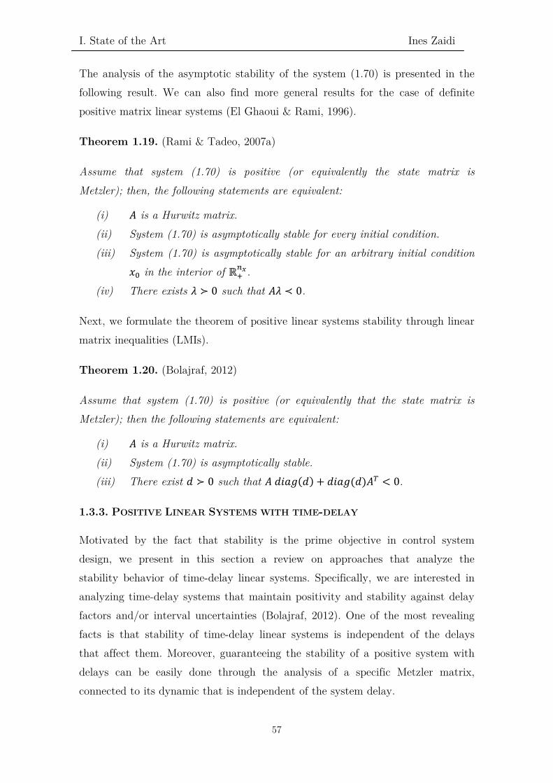
I. State of the Art Ines Zaidi
The analysis of the asymptotic stability of the system (1.70) is presented in the following result. We can also find more general results for the case of definite positive matrix linear systems (El Ghaoui & Rami, 1996).
Theorem 1.19. (Rami & Tadeo, 2007a)
Assume that system (1.70) is positive (or equivalently the state matrix is Metzler); then, the following statements are equivalent:
(i) 𝐴𝐴 is a Hurwitz matrix. (ii) System (1.70) is asymptotically stable for every initial condition. (iii) System (1.70) is asymptotically stable for an arbitrary initial condition
𝑥𝑥0 in the interior of ℝ+𝑛𝑛𝑥𝑥.
(iv) There exists 𝜆𝜆 ≻ 0 such that 𝐴𝐴𝜆𝜆 ≺ 0.
Next, we formulate the theorem of positive linear systems stability through linear matrix inequalities (LMIs).
Theorem 1.20. (Bolajraf, 2012)
Assume that system (1.70) is positive (or equivalently that the state matrix is Metzler); then the following statements are equivalent:
(i) 𝐴𝐴 is a Hurwitz matrix. (ii) System (1.70) is asymptotically stable. (iii) There exist 𝑑𝑑 ≻ 0 such that 𝐴𝐴 𝑑𝑑𝑖𝑖𝑑𝑑𝑑𝑑(𝑑𝑑) + 𝑑𝑑𝑖𝑖𝑑𝑑𝑑𝑑(𝑑𝑑)𝐴𝐴𝑇𝑇 < 0.
1.3.3. POSITIVE LINEAR SYSTEMS WITH TIME-DELAY
Motivated by the fact that stability is the prime objective in control system design, we present in this section a review on approaches that analyze the stability behavior of time-delay linear systems. Specifically, we are interested in analyzing time-delay systems that maintain positivity and stability against delay factors and/or interval uncertainties (Bolajraf, 2012). One of the most revealing facts is that stability of time-delay linear systems is independent of the delays that affect them. Moreover, guaranteeing the stability of a positive system with delays can be easily done through the analysis of a specific Metzler matrix, connected to its dynamic that is independent of the system delay.
57

I. State of the Art Ines Zaidi
We will focus on the main stability results (Bolajraf et al, 2009), (Bolajraf et al, 2010) on linear time-delay positive systems. We will also define the robust 𝛼𝛼-stability that guarantees a specified decay rate in front of possible uncertainties on the system. In addition, necessary and sufficient conditions will be provided for the stabilization of this type of systems by means of state-feedback laws that can be with or without memory.
1.3.3.1. Stability Analysis
• Asymptotic Stability
In this section, we revise necessary and sufficient stability conditions which are presented in terms of LP or LMI conditions.
Consider the class of autonomous linear system with delays, represented as follows:
�̇�𝑥(𝑡𝑡) = 𝐴𝐴𝑥𝑥(𝑡𝑡) + � 𝐴𝐴𝑚𝑚
𝑚𝑚
𝑚𝑚=1
𝑥𝑥(𝑡𝑡 − 𝜏𝜏𝑚𝑚) (1.71)
where 𝑥𝑥(𝑡𝑡) ∈ ℝ𝑛𝑛𝑥𝑥 is the state, 𝐴𝐴 ∈ ℝ𝑛𝑛𝑥𝑥×𝑛𝑛𝑥𝑥, 𝐴𝐴𝑚𝑚 ∈ ℝ𝑛𝑛𝑥𝑥×𝑛𝑛𝑥𝑥, 𝑖𝑖 = 1, … , 𝐼𝐼 are constant matrices and 𝜏𝜏𝑚𝑚, 𝑖𝑖 = 1, … , 𝐼𝐼 are constant delays.
Initial conditions are given by:
𝑥𝑥(𝑡𝑡) = 𝜙𝜙(𝑡𝑡) ∈ ℝ+𝑛𝑛𝑥𝑥, 𝑡𝑡 ∈ [−𝜏𝜏, 0], 𝜏𝜏 = max1≤𝑚𝑚≤𝑚𝑚 𝜏𝜏𝑚𝑚 (1.72)
According to Definition 1.11., the following result provides checkable conditions for the positivity of system (1.71). We can cite, for example, (Haddad & Chellaboina, 2004) and (Rami, 2009).
Proposition 1.1.
System (1.71) is positive if and only if 𝐴𝐴 is a Metzler matrix and 𝐴𝐴𝑚𝑚, 𝑖𝑖 = 1, … , 𝐼𝐼 are nonnegative matrices.
Next, necessary and sufficient conditions regarding the stability of system (1.71) are given. We can refer to some works: (Hmamed et al, 2008a), (Rami, 2009) and (Liu, 2009).
Theorem 1.21. (Bolajraf, 2012)
58

I. State of the Art Ines Zaidi
System (1.71) is asymptotically stable for every initial condition (1.72) if and only if there exists 𝜆𝜆 ∈ ℝ𝑛𝑛𝑥𝑥 such that:
�𝐴𝐴 + � 𝐴𝐴𝑚𝑚
𝑚𝑚
𝑚𝑚=1
� 𝜆𝜆 ≺ 0, 𝜆𝜆 ≻ 0 (1.73)
Remark 1.2.
We can note that checking the asymptotic stability of system (1.72) is equivalent to checking the asymptotic stability of the following positive system without delays �̇�𝑥(𝑡𝑡) = 𝐴𝐴0𝑥𝑥(𝑡𝑡), with:
𝐴𝐴0 = 𝐴𝐴 + � 𝐴𝐴𝑚𝑚
𝑚𝑚
𝑚𝑚=1
.
Corollary 1.1.
The system (1.71) is asymptotically stable for every nonnegative intial condition (1.72) if and only if one of the following conditions holds :
i) The inverse of 𝐴𝐴 + ∑ 𝐴𝐴𝑚𝑚𝑚𝑚1=1 exists and all its components are nonnegative; that
is
(𝐴𝐴 + � 𝐴𝐴𝑚𝑚
𝑚𝑚
𝑚𝑚=1
)−1 ≼ 0 (1.74)
ii) There exists 𝜆𝜆 ∈ ℝ𝑛𝑛such that
��𝐴𝐴 + � 𝐴𝐴𝑚𝑚
𝑚𝑚
𝑚𝑚=1
� 𝜆𝜆 ≺ 0
𝜆𝜆 ≻ 0
(1.75)
iii) There exists 𝑑𝑑 ∈ ℝ𝑛𝑛 such that
��𝐴𝐴 + � 𝐴𝐴𝑚𝑚
𝑚𝑚
𝑚𝑚=1
� 𝑑𝑑𝑖𝑖𝑑𝑑𝑑𝑑(𝑑𝑑) + 𝑑𝑑𝑖𝑖𝑑𝑑𝑑𝑑(𝑑𝑑) �𝐴𝐴𝑇𝑇 + � 𝐴𝐴𝑚𝑚𝑇𝑇
𝑚𝑚
𝑚𝑚=1
� < 0
𝑑𝑑 ≻ 0
(1.76)
iv) The matrix 𝐴𝐴 + ∑ 𝐴𝐴𝑚𝑚𝑝𝑝𝑚𝑚=1 is Hurwitz.
• 𝜶𝜶-Stability
59

I. State of the Art Ines Zaidi
If system (1.71) is asymptotically stable then it will decrease exponentially to the origin with a decay rate which is inherent from its dynamic. In this part, we show how one can check that the decay rate of convergence of the system is higher than a given decay rate 𝛼𝛼 which will generate a lower bound on the real decay rate of the system.
Definition 1.13.
For a real scalar 𝛼𝛼 > 0, the system (1.71) is 𝛼𝛼-stable, if all its possible trajectories satisfy lim𝑡𝑡→∞ 𝑒𝑒𝛼𝛼𝑡𝑡 𝑥𝑥(𝑡𝑡) = 0. In this case, we say that system (1.71) has at least a decay rate of order 𝛼𝛼.
Theorem 1.22.
For a real scalar 𝛼𝛼 > 0, the system (1.71) is 𝛼𝛼-stable if and only if one of the following conditions holds:
i) The positive system with delays (1.71) is asymptotically stable.
ii) There exists 𝜆𝜆 ∈ ℝ𝑛𝑛 such that
��𝐴𝐴 + 𝛼𝛼𝐼𝐼 + � 𝑒𝑒𝛼𝛼𝜏𝜏𝑖𝑖𝐴𝐴𝑚𝑚
𝑚𝑚
𝑚𝑚=1
� 𝜆𝜆 ≺ 0
𝜆𝜆 ≻ 0
(1.77)
iii) There exists 𝑑𝑑 ∈ ℝ𝑛𝑛 such that
��𝐴𝐴 + � 𝑒𝑒𝛼𝛼𝜏𝜏𝑖𝑖𝐴𝐴𝑚𝑚
𝑚𝑚
𝑚𝑚=1
� 𝑑𝑑𝑖𝑖𝑑𝑑𝑑𝑑(𝑑𝑑) + 𝑑𝑑𝑖𝑖𝑑𝑑𝑑𝑑(𝑑𝑑) �𝐴𝐴𝑇𝑇 + � 𝑒𝑒𝛼𝛼𝜏𝜏𝑖𝑖𝐴𝐴𝑚𝑚𝑇𝑇
𝑚𝑚
𝑚𝑚=1
� + 2𝛼𝛼𝑑𝑑𝑖𝑖𝑑𝑑𝑑𝑑(𝑑𝑑) < 0
𝑑𝑑 ≻ 0
(1.78)
Regarding unknown delays, we can extend the previous result.
Corollary 1.2.
Assume that the time delays are unknown but bounded 0 ≤ 𝜏𝜏𝑚𝑚 ≤ 𝜏𝜏, 𝑖𝑖 = 1, … , 𝐼𝐼. Then, for a given real scalar 𝛼𝛼 > 0, the following statements are equivalent.
i) The positive system (1.71) is 𝛼𝛼-stable for any delays bounded by 𝜏𝜏.
ii) There exists 𝜆𝜆 ∈ ℝ𝑛𝑛 such that
60

I. State of the Art Ines Zaidi
��𝐴𝐴 + 𝛼𝛼𝐼𝐼 + 𝑒𝑒𝛼𝛼𝜏𝜏 � 𝐴𝐴𝑚𝑚
𝑚𝑚
𝑚𝑚=1
� 𝜆𝜆 ≺ 0
𝜆𝜆 ≻ 0
(1.79)
iii) There exists 𝑑𝑑 ∈ ℝ𝑛𝑛 such that
� �𝐴𝐴 + 𝑒𝑒𝛼𝛼𝜏𝜏 � 𝐴𝐴𝑚𝑚
𝑚𝑚
𝑚𝑚=1
� 𝑑𝑑𝑖𝑖𝑑𝑑𝑑𝑑(𝑑𝑑) + 𝑑𝑑𝑖𝑖𝑑𝑑𝑑𝑑(𝑑𝑑) �𝐴𝐴𝑇𝑇 + 𝑒𝑒𝛼𝛼𝜏𝜏 � 𝐴𝐴𝑚𝑚𝑇𝑇
𝑚𝑚
𝑚𝑚=1
� + 2𝛼𝛼𝑑𝑑𝑖𝑖𝑑𝑑𝑑𝑑(𝑑𝑑) < 0
𝑑𝑑 ≻ 0
(1.80)
1.3.3.2. PDC Controller Design
Consider the following forced time-delay system:
�̇�𝑥(𝑡𝑡) = 𝐴𝐴𝑥𝑥(𝑡𝑡) + � 𝐴𝐴𝑚𝑚
𝑚𝑚
𝑚𝑚=1
𝑥𝑥(𝑡𝑡 − 𝜏𝜏𝑚𝑚) + 𝐵𝐵𝑢𝑢(𝑡𝑡) (1.81)
where 𝑥𝑥(𝑡𝑡) ∈ ℝ𝑛𝑛𝑥𝑥 is the state, 𝑢𝑢(𝑡𝑡) ∈ ℝ𝑛𝑛𝑢𝑢 is the control input and 𝜏𝜏𝑚𝑚, 𝑖𝑖 = 1, … , 𝐼𝐼 are the delays. Matrices 𝐴𝐴 ∈ ℝ𝑛𝑛𝑥𝑥×𝑛𝑛𝑥𝑥, 𝐵𝐵 ∈ ℝ𝑛𝑛𝑥𝑥×𝑛𝑛𝑢𝑢 represent the nominal system without delays. 𝐴𝐴𝑚𝑚, 𝑖𝑖 = 1, … , 𝐼𝐼 are known matrices and the initial condition is given by (1.72).
We are meant to design for system (1.71) a state-feedback controller of the form:
𝑢𝑢(𝑡𝑡) = 𝐾𝐾𝑥𝑥(𝑡𝑡), 𝐾𝐾 ∈ ℝ𝑛𝑛𝑢𝑢×𝑛𝑛𝑥𝑥 (1.82)
For which the closed-loop system is positive and asymptotically stable.
Applying the control law (1.82) to system (1.71), we get the closed-loop system given by:
�̇�𝑥(𝑡𝑡) = (𝐴𝐴 + 𝐵𝐵𝐾𝐾)𝑥𝑥(𝑡𝑡) + � 𝐴𝐴𝑚𝑚
𝑚𝑚
𝑚𝑚=1
𝑥𝑥(𝑡𝑡 − 𝜏𝜏𝑚𝑚) (1.83)
Hence, we need to find necessary and sufficient conditions on matrices 𝐴𝐴, 𝐴𝐴1,…,𝐴𝐴𝑚𝑚 and 𝐵𝐵, such that there exists a matrix 𝐾𝐾 satisfying:
* Positivity of the closed-loop system: the matrix 𝐴𝐴 + 𝐵𝐵𝐾𝐾 is Metzler (𝐴𝐴1,…,𝐴𝐴𝑚𝑚) are necessarily nonnegative)
* Stability of the closed-loop system: the matrix 𝐴𝐴 + 𝐵𝐵𝐾𝐾 is Hurwitz.
• State-feedback 𝜶𝜶-Stabilization
61

I. State of the Art Ines Zaidi
In the folowing, we develop necessary and sufficient conditions for positivity and 𝛼𝛼-stability of the closed-loop system (1.83).
Theorem 1.23. (Bolajraf, 2012)
Assume that the matrices 𝐴𝐴𝑚𝑚, 𝑖𝑖 = 1, … , 𝐼𝐼 are nonnegative. Then, for a prescribed decay rate 𝛼𝛼 > 0, the closed-loop system (1.83) is positive and 𝛼𝛼-stable if and only if one of the following equivalent conditions is satisfied :
i) The following LP problem in the variables 𝛽𝛽 ∈ ℝ+, 𝜆𝜆 ∈ ℝ+𝑛𝑛𝑥𝑥 and 𝑍𝑍 ∈ ℝ𝑛𝑛𝑥𝑥×𝑛𝑛𝑢𝑢 is
feasible
�𝐴𝐴0𝜆𝜆 + 𝐵𝐵𝑍𝑍1𝑛𝑛𝑥𝑥 < 0 𝐴𝐴𝑑𝑑𝑖𝑖𝑑𝑑𝑑𝑑(𝜆𝜆) + 𝐵𝐵𝑍𝑍 + 𝛽𝛽1𝑛𝑛𝑥𝑥
𝜆𝜆 > 0 ≽ 0 (1.84)
where:
𝐴𝐴0 = 𝐴𝐴 + 𝛼𝛼𝐼𝐼 + � 𝑒𝑒𝛼𝛼𝜏𝜏𝑖𝑖𝐴𝐴𝑚𝑚
𝑚𝑚
𝑚𝑚=1
Moreover, the gain matrix 𝐾𝐾 satisfying (1.84) can be computed as follows
𝐾𝐾 = 𝑍𝑍𝑑𝑑𝑖𝑖𝑑𝑑𝑑𝑑(𝜆𝜆)−1 (1.85)
where 𝜆𝜆 and 𝑍𝑍 are any feasible solution to the LP problem (1.84).
ii) The following LMI problem in the variables 𝛽𝛽 ∈ ℝ+, 𝑑𝑑 ∈ ℝ𝑛𝑛𝑥𝑥 and 𝑌𝑌 ∈ ℝ𝑛𝑛𝑥𝑥×𝑛𝑛𝑢𝑢 is feasible
�𝐴𝐴0𝑑𝑑𝑖𝑖𝑑𝑑𝑑𝑑(𝑑𝑑) + 𝑑𝑑𝑖𝑖𝑑𝑑𝑑𝑑(𝑑𝑑)𝐴𝐴0
𝑇𝑇 + 𝐵𝐵𝑌𝑌 + 𝑌𝑌𝑇𝑇𝐵𝐵𝑇𝑇 < 0 𝐴𝐴𝑑𝑑𝑖𝑖𝑑𝑑𝑑𝑑(𝑑𝑑) + 𝐵𝐵𝑌𝑌 + 𝛽𝛽𝐼𝐼𝑛𝑛𝑥𝑥 ≽ 0 𝑑𝑑 > 0
(1.86)
Moreover, the gain matrix 𝐾𝐾 satisfying (1.86) can be computed as follows
𝐾𝐾 = 𝑌𝑌𝑑𝑑𝑖𝑖𝑑𝑑𝑑𝑑(𝑑𝑑)−1 (1.87)
where 𝑑𝑑 and 𝑌𝑌 are any feasible solution to the LMI problem (1.86).
Results on robust stabilization and estimation of postive interval systems are also studied in (Bolajraf, 2012).
1.3.4. POSITIVE TAKAGI-SUGENO SYSTEMS
62
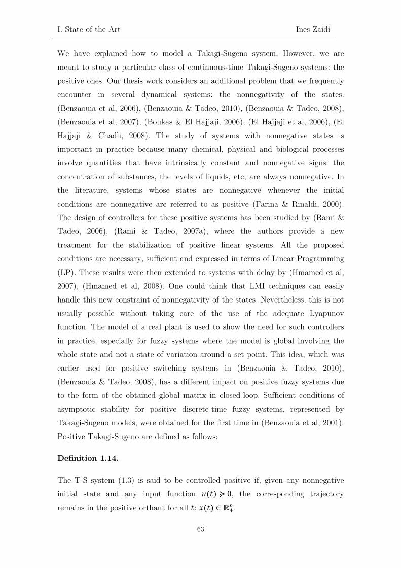
I. State of the Art Ines Zaidi
We have explained how to model a Takagi-Sugeno system. However, we are meant to study a particular class of continuous-time Takagi-Sugeno systems: the positive ones. Our thesis work considers an additional problem that we frequently encounter in several dynamical systems: the nonnegativity of the states. (Benzaouia et al, 2006), (Benzaouia & Tadeo, 2010), (Benzaouia & Tadeo, 2008), (Benzaouia et al, 2007), (Boukas & El Hajjaji, 2006), (El Hajjaji et al, 2006), (El Hajjaji & Chadli, 2008). The study of systems with nonnegative states is important in practice because many chemical, physical and biological processes involve quantities that have intrinsically constant and nonnegative signs: the concentration of substances, the levels of liquids, etc, are always nonnegative. In the literature, systems whose states are nonnegative whenever the initial conditions are nonnegative are referred to as positive (Farina & Rinaldi, 2000). The design of controllers for these positive systems has been studied by (Rami & Tadeo, 2006), (Rami & Tadeo, 2007a), where the authors provide a new treatment for the stabilization of positive linear systems. All the proposed conditions are necessary, sufficient and expressed in terms of Linear Programming (LP). These results were then extended to systems with delay by (Hmamed et al, 2007), (Hmamed et al, 2008). One could think that LMI techniques can easily handle this new constraint of nonnegativity of the states. Nevertheless, this is not usually possible without taking care of the use of the adequate Lyapunov function. The model of a real plant is used to show the need for such controllers in practice, especially for fuzzy systems where the model is global involving the whole state and not a state of variation around a set point. This idea, which was earlier used for positive switching systems in (Benzaouia & Tadeo, 2010), (Benzaouia & Tadeo, 2008), has a different impact on positive fuzzy systems due to the form of the obtained global matrix in closed-loop. Sufficient conditions of asymptotic stability for positive discrete-time fuzzy systems, represented by Takagi-Sugeno models, were obtained for the first time in (Benzaouia et al, 2001). Positive Takagi-Sugeno are defined as follows:
Definition 1.14.
The T-S system (1.3) is said to be controlled positive if, given any nonnegative initial state and any input function 𝑢𝑢(𝑡𝑡) ≽ 0, the corresponding trajectory remains in the positive orthant for all 𝑡𝑡: 𝑥𝑥(𝑡𝑡) ∈ ℝ+
𝑛𝑛 .
63

I. State of the Art Ines Zaidi
Lemma 1.2.
The autonomous system (1.3) is positive if and only if 𝐴𝐴𝑚𝑚 is a Metzler matrix and 𝐵𝐵𝑚𝑚, 𝐶𝐶𝑚𝑚 and 𝐷𝐷𝑚𝑚 are nonnegative matrices for 𝑖𝑖 = 1, … , 𝑟𝑟.
Next, in the following chapters, we will deal with the stabilization and estimation of positive T-S systems.
1.3.5. REVIEW ON POSITIVE TIME-DELAY TAKAGI-SUGENO SYSTEMS
However, a new constraint is added to this type of systems: the positivity. The aim becomes then to maintain the stability and positivity of the states at each time.
Consider a nonlinear system with time-delay which could be represented by a T-S time-delay model described by (1.43).
Then, the overall T-S system can be inferred as:
�̇�𝑥(𝑡𝑡) = � ℎ𝑚𝑚�𝑧𝑧(𝑡𝑡)� �𝐴𝐴𝑚𝑚𝑥𝑥(𝑡𝑡) + 𝐴𝐴1𝑚𝑚𝑥𝑥�𝑡𝑡 − 𝜏𝜏(𝑡𝑡)� + 𝐵𝐵𝑚𝑚𝑢𝑢(𝑡𝑡)� 𝑟𝑟
𝑚𝑚=1
(1.88)
such that (1.4) is satisfied.
Definition 1.15.
The T-S system (1.88) is said to be controlled positive if, given any nonnegative initial state and any input function 𝑢𝑢(𝑡𝑡) ≽ 0, the corresponding trajectory remains in the positive orthant for all 𝑡𝑡, 𝑥𝑥 ∈ ℝ+
𝑛𝑛 .
Lemma 1.3. (Benzaouia et al, 2011)
The autonomous delayed system (1.88) is positive if and only if 𝐴𝐴𝑚𝑚 is a Metzler matrix and 𝐴𝐴1𝑚𝑚 and 𝐵𝐵𝑚𝑚 are nonnegative matrices for 𝑖𝑖 = 1, … , 𝑟𝑟.
Conditions of stability and stabilization of a time-delay T-S system (1.88), using LMI method as presented in (Benzaouia et al, 2011), are recalled.
Theorem 1.24.
64
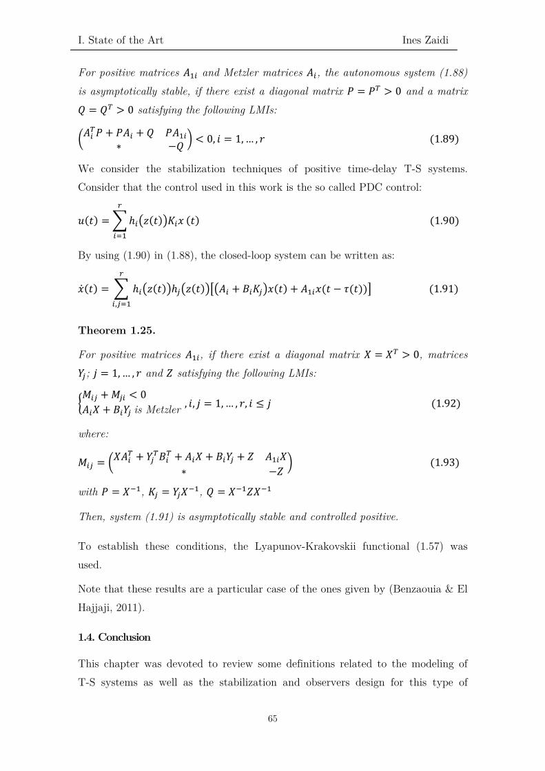
I. State of the Art Ines Zaidi
For positive matrices 𝐴𝐴1𝑚𝑚 and Metzler matrices 𝐴𝐴𝑚𝑚, the autonomous system (1.88) is asymptotically stable, if there exist a diagonal matrix 𝑃𝑃 = 𝑃𝑃𝑇𝑇 > 0 and a matrix 𝑄𝑄 = 𝑄𝑄𝑇𝑇 > 0 satisfying the following LMIs:
�𝐴𝐴𝑚𝑚𝑇𝑇𝑃𝑃 + 𝑃𝑃𝐴𝐴𝑚𝑚 + 𝑄𝑄 𝑃𝑃𝐴𝐴1𝑚𝑚
∗ −𝑄𝑄 � < 0, 𝑖𝑖 = 1, … , 𝑟𝑟 (1.89)
We consider the stabilization techniques of positive time-delay T-S systems. Consider that the control used in this work is the so called PDC control:
𝑢𝑢(𝑡𝑡) = � ℎ𝑚𝑚�𝑧𝑧(𝑡𝑡)�𝐾𝐾𝑚𝑚𝑥𝑥𝑟𝑟
𝑚𝑚=1
(𝑡𝑡) (1.90)
By using (1.90) in (1.88), the closed-loop system can be written as:
�̇�𝑥(𝑡𝑡) = � ℎ𝑚𝑚�𝑧𝑧(𝑡𝑡)�ℎ𝑖𝑖�𝑧𝑧(𝑡𝑡)���𝐴𝐴𝑚𝑚 + 𝐵𝐵𝑚𝑚𝐾𝐾𝑖𝑖�𝑥𝑥(𝑡𝑡) + 𝐴𝐴1𝑚𝑚𝑥𝑥(𝑡𝑡 − 𝜏𝜏(𝑡𝑡))�𝑟𝑟
𝑚𝑚,𝑖𝑖=1
(1.91)
Theorem 1.25.
For positive matrices 𝐴𝐴1𝑚𝑚, if there exist a diagonal matrix 𝑋𝑋 = 𝑋𝑋𝑇𝑇 > 0, matrices 𝑌𝑌𝑖𝑖; 𝑗𝑗 = 1, … , 𝑟𝑟 and 𝑍𝑍 satisfying the following LMIs:
�𝑀𝑀𝑚𝑚𝑖𝑖 + 𝑀𝑀𝑖𝑖𝑚𝑚 < 0 𝐴𝐴𝑚𝑚𝑋𝑋 + 𝐵𝐵𝑚𝑚𝑌𝑌𝑖𝑖 is Metzler , 𝑖𝑖, 𝑗𝑗 = 1, … , 𝑟𝑟, 𝑖𝑖 ≤ 𝑗𝑗 (1.92)
where:
𝑀𝑀𝑚𝑚𝑖𝑖 = �𝑋𝑋𝐴𝐴𝑚𝑚𝑇𝑇 + 𝑌𝑌𝑖𝑖
𝑇𝑇𝐵𝐵𝑚𝑚𝑇𝑇 + 𝐴𝐴𝑚𝑚𝑋𝑋 + 𝐵𝐵𝑚𝑚𝑌𝑌𝑖𝑖 + 𝑍𝑍 𝐴𝐴1𝑚𝑚𝑋𝑋
∗ −𝑍𝑍� (1.93)
with 𝑃𝑃 = 𝑋𝑋−1, 𝐾𝐾𝑖𝑖 = 𝑌𝑌𝑖𝑖𝑋𝑋−1, 𝑄𝑄 = 𝑋𝑋−1𝑍𝑍𝑋𝑋−1
Then, system (1.91) is asymptotically stable and controlled positive.
To establish these conditions, the Lyapunov-Krakovskii functional (1.57) was used.
Note that these results are a particular case of the ones given by (Benzaouia & El Hajjaji, 2011).
1.4. Conclusion
This chapter was devoted to review some definitions related to the modeling of T-S systems as well as the stabilization and observers design for this type of
65

I. State of the Art Ines Zaidi
systems, taking into account if the decision variables are measurable or not. Recent approaches have been presented. A discussion of nonlinear systems was then used to introduce T-S models with time-delay, presenting briefly the classification of delay models and time-delay T-S models. We have also introduced methods for the stabilization and estimation of this class of systems. Finally, we have presented useful properties and results about positive dynamic systems. In particular, we have analyzed positivity and stability of linear systems and we have provided necessary and sufficient conditions for their stabilization. Equivalent conditions for checking 𝛼𝛼-stability have been given in terms of LP and LMIs. These results were applied for the control design of positive systems with time-delays. Then, we made a short background on positive T-S time-delay systems. The previous results will be useful for the several approaches of the next chapters.
66

I. State of the Art Ines Zaidi
67

II. Stability and Stabilization of Positive T-S systems Ines Zaidi
68

II. Stability and Stabilization of Positive T-S systems Ines Zaidi
Chapter II
Stability and Stabilization of Positive Takagi-Sugeno systems
69

II. Stability and Stabilization of Positive T-S systems Ines Zaidi
70

II. Stability and Stabilization of Positive T-S systems Ines Zaidi
2.1. Introduction
In this chapter, we are interested in the analysis of stability and stabilization of positive dynamical systems. Regarding linear systems, we may recall some basic properties of positive systems, developed in (Luenberger, 1979). Other structural and stability properties can be found in (Farina & Rinaldi, 2000). More investigation works were developed in this issue (Kaczorek, 2002), (Haddad et al, 2010), (Benzaouia et al, 2010), (Benzaouia et al, 2011), etc. For this, we will provide our results for positive T-S systems. We note that positive linear systems are a particular case of positive Takagi-Sugeno systems.
2.2. Stability and Stabilization of Positive Takagi-Sugeno systems with measurable premise variables
Control synthesis for the systems that are represented by Takagi-Sugeno (T-S) models may be considered as a convex problem soluble by LMI optimization techniques (Kim & Park, 2003). Despite the benefits of LMIs, the existence of a solution which satisfies the sufficient stabilization conditions is not always guaranteed, specially, when the number of submodels increases, or when several constraints are imposed on the control performance such as the convergence rate, the problem becomes unsolvable (Luoh, 2002).
To overcome this problem, several studies have proposed less stringent stabilization conditions to minimize the conservatism of these techniques (Tanaka et al, 1998), (Lim & Lee, 2000), (Xiaodong & Qingling, 2003), (Chadli et al, 2004). However, maximizing the speed of convergence is often not considered.
An extension of this work was proposed to define new conditions of asymptotic and exponential stability with maximization of the convergence rate for a Takagi-Sugeno system with measurable variable decisions. In addition to the LMIs, other optimization techniques have been used, such as the resolution of the problem of generalized eigenvalues (GEVP) and the maximization of a function under constraints (Salem, 2013).
After a presentation of the results established in the literature regarding the stability of T-S systems, new and improved conditions for both continuous and discrete systems are proposed. These conditions are then used for the synthesis of
71
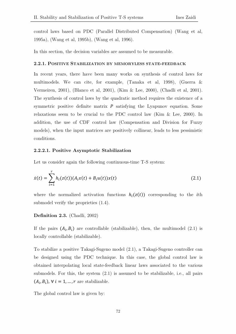
II. Stability and Stabilization of Positive T-S systems Ines Zaidi
control laws based on PDC (Parallel Distributed Compensation) (Wang et al, 1995a), (Wang et al, 1995b), (Wang et al, 1996).
In this section, the decision variables are assumed to be measurable.
2.2.1. POSITIVE STABILIZATION BY MEMORYLESS STATE-FEEDBACK
In recent years, there have been many works on synthesis of control laws for multimodels. We can cite, for example, (Tanaka et al, 1998), (Guerra & Vermeiren, 2001), (Blanco et al, 2001), (Kim & Lee, 2000), (Chadli et al, 2001). The synthesis of control laws by the quadratic method requires the existence of a symmetric positive definite matrix 𝑃𝑃 satisfying the Lyapunov equation. Some relaxations seem to be crucial to the PDC control law (Kim & Lee, 2000). In addition, the use of CDF control law (Compensation and Division for Fuzzy models), when the input matrices are positively collinear, leads to less pessimistic conditions.
2.2.2.1. Positive Asymptotic Stabilization
Let us consider again the following continuous-time T-S system:
�̇�𝑥(𝑡𝑡) = � ℎ𝑚𝑚(𝑧𝑧(𝑡𝑡))(𝐴𝐴𝑚𝑚𝑥𝑥(𝑡𝑡) + 𝐵𝐵𝑚𝑚𝑢𝑢(𝑡𝑡))𝑥𝑥(𝑡𝑡)𝑟𝑟
𝑚𝑚=1
(2.1)
where the normalized activation functions ℎ𝑚𝑚(𝑧𝑧(𝑡𝑡)) corresponding to the 𝑖𝑖th submodel verify the proprieties (1.4).
Definition 2.3. (Chadli, 2002)
If the pairs (𝐴𝐴𝑚𝑚 , 𝐵𝐵𝑚𝑚) are controllable (stabilizable), then, the multimodel (2.1) is locally controllable (stabilizable).
To stabilize a positive Takagi-Sugeno model (2.1), a Takagi-Sugeno controller can be designed using the PDC technique. In this case, the global control law is obtained interpolating local state-feedback linear laws associated to the various submodels. For this, the system (2.1) is assumed to be stabilizable, i.e., all pairs (𝐴𝐴𝑚𝑚, 𝐵𝐵𝑚𝑚), ∀ 𝑖𝑖 = 1, … , 𝑟𝑟 are stabilizable.
The global control law is given by:
72

II. Stability and Stabilization of Positive T-S systems Ines Zaidi
𝑢𝑢(𝑡𝑡) = − � ℎ𝑚𝑚�𝑧𝑧(𝑡𝑡)�𝐾𝐾𝑚𝑚𝑥𝑥(𝑡𝑡)𝑟𝑟
𝑚𝑚=1
(2.2)
where ℎ𝑚𝑚(𝑧𝑧(𝑡𝑡)) are the activation functions verifying the constraints (2.2).
Substituting (2.2) in (2.1), we obtain the continuous-time closed loop system:
�̇�𝑥(𝑡𝑡) = � ℎ𝑚𝑚(𝑧𝑧(𝑡𝑡))ℎ𝑖𝑖(𝑧𝑧(𝑡𝑡))𝐺𝐺𝑚𝑚𝑖𝑖𝑥𝑥(𝑡𝑡)𝑟𝑟
𝑚𝑚,𝑖𝑖=1
(2.3)
= � ℎ𝑚𝑚2�𝑧𝑧(𝑡𝑡)�𝐺𝐺𝑚𝑚𝑚𝑚𝑥𝑥(𝑡𝑡) + 2 � ℎ𝑚𝑚�𝑧𝑧(𝑡𝑡)�ℎ𝑖𝑖�𝑧𝑧(𝑡𝑡)� �
𝐺𝐺𝑚𝑚𝑖𝑖 + 𝐺𝐺𝑖𝑖𝑚𝑚
2� 𝑥𝑥(𝑡𝑡)
𝑟𝑟
1≤𝑚𝑚<𝑖𝑖
𝑟𝑟
𝑚𝑚=1
(2.4)
where: 𝐺𝐺𝑚𝑚𝑖𝑖 = 𝐴𝐴𝑚𝑚 − 𝐵𝐵𝑚𝑚𝐾𝐾𝑖𝑖 (2.5)
The equation (2.4) highlights the submodels called dominant characterized by the
matrices 𝐺𝐺𝑚𝑚𝑚𝑚 and the submodels called couples caracterized by �𝐺𝐺𝑖𝑖𝑖𝑖+𝐺𝐺𝑖𝑖𝑖𝑖
2�.
We then use (2.4) the previous results to analyse the stability of positive Takagi-Sugeno systems, as an extension of (Chadli, 2002) for positive T-S systems.
Theorem 2.1.
The system described by (2.4) is globally asymptotically stable and positive, if there exist a symmetric positive definite matrix 𝑃𝑃 and a positive scalar 𝛽𝛽 such
that:
⎩⎪⎨
⎪⎧ 𝐺𝐺𝑚𝑚𝑚𝑚
𝑇𝑇𝑃𝑃 + 𝑃𝑃𝐺𝐺𝑚𝑚𝑚𝑚 < 0; 1 ≤ 𝑖𝑖 ≤ 𝑟𝑟
�𝐺𝐺𝑚𝑚𝑖𝑖 + 𝐺𝐺𝑖𝑖𝑚𝑚
2�
𝑇𝑇
𝑃𝑃 + 𝑃𝑃 �𝐺𝐺𝑚𝑚𝑖𝑖 + 𝐺𝐺𝑖𝑖𝑚𝑚
2� ≤ 0; 1 ≤ 𝑖𝑖 < 𝑗𝑗 ≤ 𝑟𝑟
𝐺𝐺𝑚𝑚𝑖𝑖𝑃𝑃 + 𝛽𝛽𝑃𝑃 ≽ 0
(2.6)
Proof:
The first two conditions in Theorem 2.1. are given from (Chadli, 2002). Moreover, to guarantee the positivity of the closed-loop system (2.4), we have to prove that 𝐺𝐺𝑚𝑚𝑖𝑖 = 𝐴𝐴𝑚𝑚 − 𝐵𝐵𝑚𝑚𝐾𝐾𝑖𝑖 is Metzler, ∀ 𝑖𝑖, 𝑗𝑗 = 1, … , 𝑟𝑟: From Remark 1.1, (2.4) is positive if
and only if there exists 𝛽𝛽 ∈ ℝ+ such that �𝐺𝐺𝑚𝑚𝑖𝑖 + 𝛽𝛽𝐼𝐼� ≽ 0 (2.7)
Multiplying this inequality on the right by 𝑃𝑃, we get: 𝐺𝐺𝑚𝑚𝑖𝑖𝑃𝑃 + 𝛽𝛽𝑃𝑃 ≽ 0. This ends
the proof. ∎
73
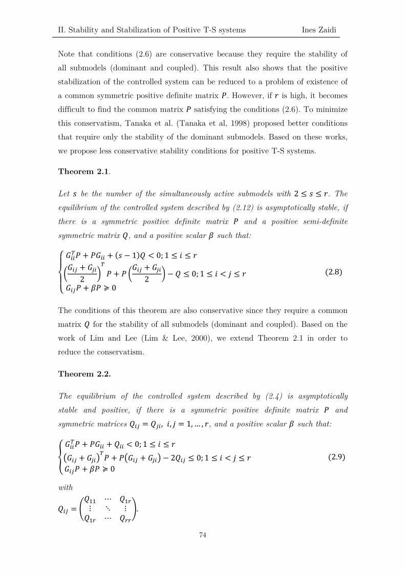
II. Stability and Stabilization of Positive T-S systems Ines Zaidi
Note that conditions (2.6) are conservative because they require the stability of all submodels (dominant and coupled). This result also shows that the positive stabilization of the controlled system can be reduced to a problem of existence of a common symmetric positive definite matrix 𝑃𝑃. However, if 𝑟𝑟 is high, it becomes difficult to find the common matrix 𝑃𝑃 satisfying the conditions (2.6). To minimize this conservatism, Tanaka et al. (Tanaka et al, 1998) proposed better conditions that require only the stability of the dominant submodels. Based on these works, we propose less conservative stability conditions for positive T-S systems.
Theorem 2.1.
Let 𝑠𝑠 be the number of the simultaneously active submodels with 2 ≤ 𝑠𝑠 ≤ 𝑟𝑟. The equilibrium of the controlled system described by (2.12) is asymptotically stable, if there is a symmetric positive definite matrix 𝑃𝑃 and a positive semi-definite
symmetric matrix 𝑄𝑄, and a positive scalar 𝛽𝛽 such that:
⎩⎪⎨
⎪⎧ 𝐺𝐺𝑚𝑚𝑚𝑚
𝑇𝑇𝑃𝑃 + 𝑃𝑃𝐺𝐺𝑚𝑚𝑚𝑚 + (𝑠𝑠 − 1)𝑄𝑄 < 0; 1 ≤ 𝑖𝑖 ≤ 𝑟𝑟
�𝐺𝐺𝑚𝑚𝑖𝑖 + 𝐺𝐺𝑖𝑖𝑚𝑚
2�
𝑇𝑇
𝑃𝑃 + 𝑃𝑃 �𝐺𝐺𝑚𝑚𝑖𝑖 + 𝐺𝐺𝑖𝑖𝑚𝑚
2� − 𝑄𝑄 ≤ 0; 1 ≤ 𝑖𝑖 < 𝑗𝑗 ≤ 𝑟𝑟
𝐺𝐺𝑚𝑚𝑖𝑖𝑃𝑃 + 𝛽𝛽𝑃𝑃 ≽ 0
(2.8)
The conditions of this theorem are also conservative since they require a common matrix 𝑄𝑄 for the stability of all submodels (dominant and coupled). Based on the work of Lim and Lee (Lim & Lee, 2000), we extend Theorem 2.1 in order to reduce the conservatism.
Theorem 2.2.
The equilibrium of the controlled system described by (2.4) is asymptotically stable and positive, if there is a symmetric positive definite matrix 𝑃𝑃 and symmetric matrices 𝑄𝑄𝑚𝑚𝑖𝑖 = 𝑄𝑄𝑖𝑖𝑚𝑚 , 𝑖𝑖, 𝑗𝑗 = 1, … , 𝑟𝑟, and a positive scalar 𝛽𝛽 such that:
�𝐺𝐺𝑚𝑚𝑚𝑚
𝑇𝑇𝑃𝑃 + 𝑃𝑃𝐺𝐺𝑚𝑚𝑚𝑚 + 𝑄𝑄𝑚𝑚𝑚𝑚 < 0; 1 ≤ 𝑖𝑖 ≤ 𝑟𝑟
�𝐺𝐺𝑚𝑚𝑖𝑖 + 𝐺𝐺𝑖𝑖𝑚𝑚�𝑇𝑇
𝑃𝑃 + 𝑃𝑃�𝐺𝐺𝑚𝑚𝑖𝑖 + 𝐺𝐺𝑖𝑖𝑚𝑚� − 2𝑄𝑄𝑚𝑚𝑖𝑖 ≤ 0; 1 ≤ 𝑖𝑖 < 𝑗𝑗 ≤ 𝑟𝑟𝐺𝐺𝑚𝑚𝑖𝑖𝑃𝑃 + 𝛽𝛽𝑃𝑃 ≽ 0
(2.9)
with
𝑄𝑄𝑚𝑚𝑖𝑖 = �𝑄𝑄11 ⋯ 𝑄𝑄1𝑟𝑟
⋮ ⋱ ⋮𝑄𝑄1𝑟𝑟 ⋯ 𝑄𝑄𝑟𝑟𝑟𝑟
�.
74

II. Stability and Stabilization of Positive T-S systems Ines Zaidi
The conditions (2.9) of Theorem 2.2. impose 𝑄𝑄𝑚𝑚𝑖𝑖 = 𝑄𝑄𝑖𝑖𝑚𝑚, 𝑖𝑖 = 1, … , 𝑟𝑟 and that these
matrices are all symmetric; so we have extended the works of Xiaodong and Qingling (Xiaodong & Qingling, 2003) to improve them:
Theorem 2.3.
The equilibrium of the controlled system described by (2.4) is asymptotically stable and positive, if there is a symmetric positive definite matrix 𝑃𝑃, symmetric matrices 𝑄𝑄𝑚𝑚𝑚𝑚, ∀ 𝑖𝑖 = 1, … , 𝑟𝑟 and matrices 𝑄𝑄𝑖𝑖𝑚𝑚 = 𝑄𝑄𝑚𝑚𝑖𝑖
𝑇𝑇 , 1 ≤ 𝑖𝑖 < 𝑗𝑗 ≤ 𝑟𝑟, and a positive
scalar 𝛽𝛽 such that:
⎩⎪⎨
⎪⎧ 𝐺𝐺𝑚𝑚𝑚𝑚
𝑇𝑇𝑃𝑃 + 𝑃𝑃𝐺𝐺𝑚𝑚𝑚𝑚 + 𝑄𝑄𝑚𝑚𝑚𝑚 < 0; 1 ≤ 𝑖𝑖 ≤ 𝑟𝑟
�𝐺𝐺𝑚𝑚𝑖𝑖 + 𝐺𝐺𝑖𝑖𝑚𝑚�𝑇𝑇
𝑃𝑃 + 𝑃𝑃�𝐺𝐺𝑚𝑚𝑖𝑖 + 𝐺𝐺𝑖𝑖𝑚𝑚� + (𝑄𝑄𝑚𝑚𝑖𝑖 + 𝑄𝑄𝑚𝑚𝑖𝑖𝑇𝑇) ≤ 0; 1 ≤ 𝑖𝑖 < 𝑗𝑗 ≤ 𝑟𝑟
𝐺𝐺𝑚𝑚𝑖𝑖𝑃𝑃 + 𝛽𝛽𝑃𝑃 ≽ 0
(2.10)
with:
𝑄𝑄𝑚𝑚𝑖𝑖 = �
𝑄𝑄11 𝑄𝑄12 ⋯ 𝑄𝑄1𝑟𝑟𝑄𝑄12
𝑇𝑇 𝑄𝑄22 … 𝑄𝑄2𝑟𝑟⋮ . ⋱ ⋮
𝑄𝑄1𝑟𝑟𝑇𝑇 𝑄𝑄2𝑟𝑟
𝑇𝑇 ⋯ 𝑄𝑄𝑟𝑟𝑟𝑟
�.
2.2.2.2. Positive Exponential Stabilization
In addition to the stabilization, there exist other important control performances such as the decay rate, also called stabilization degree, defined as a scalar 𝛼𝛼 > 0 such that:
lim𝑡𝑡→∞
𝑒𝑒𝛼𝛼𝑡𝑡‖𝑥𝑥(𝑡𝑡)‖ = 0 (2.11)
for all the trajectories 𝑥𝑥(𝑡𝑡) of the system (2.4).
Condition (2.11) is guaranteed if:
�̇�𝑉�𝑥𝑥(𝑡𝑡)� ≤ −2𝛼𝛼𝑉𝑉�𝑥𝑥(𝑡𝑡)� (2.12)
where: 𝑉𝑉�𝑥𝑥(𝑡𝑡)� is a quadratic Lyapunov function with 𝑃𝑃 > 0.
Chadli et al. (Chadli et al, 2002d) have developed the global exponential stability conditions of the system (2.4) where only the dominant submodels are meant to be stable but with a common matrix 𝑄𝑄, and have characterized the minimum
75

II. Stability and Stabilization of Positive T-S systems Ines Zaidi
decay rate of the system. We have then extended the results to the positive Takagi-Sugeno systems in the following.
Theorem 2.4.
Let 𝑠𝑠 be the number of the simultaneously active submodels with 2 ≤ 𝑠𝑠 ≤ 𝑟𝑟. The equilibrium of the controlled system (2.4) is globally exponentially stable and positive if there exist two symmetric positive definite matrices 𝑃𝑃 and 𝑄𝑄, a scalar
0 < 𝜀𝜀 < 1 and a scalar 𝛽𝛽 ∈ ℝ+ such that:
⎩⎪⎨
⎪⎧ 𝐺𝐺𝑚𝑚𝑚𝑚
𝑇𝑇𝑃𝑃 + 𝑃𝑃𝐺𝐺𝑚𝑚𝑚𝑚 + (𝑠𝑠 − 𝜀𝜀)𝑄𝑄 < 0; 1 ≤ 𝑖𝑖 ≤ 𝑟𝑟
�𝐺𝐺𝑚𝑚𝑖𝑖 + 𝐺𝐺𝑖𝑖𝑚𝑚
2�
𝑇𝑇
𝑃𝑃 + 𝑃𝑃 �𝐺𝐺𝑚𝑚𝑖𝑖 + 𝐺𝐺𝑖𝑖𝑚𝑚
2� − 𝜀𝜀𝑄𝑄 ≤ 0; 1 ≤ 𝑖𝑖 < 𝑗𝑗 ≤ 𝑟𝑟
𝐺𝐺𝑚𝑚𝑖𝑖𝑃𝑃 + 𝛽𝛽𝑃𝑃 ≽ 0
(2.13)
The minimum decay rate is given by:
𝛼𝛼 = (1 − 𝜀𝜀)𝜆𝜆𝑚𝑚𝑚𝑚𝑛𝑛(𝑄𝑄)
2𝜆𝜆𝑚𝑚𝑚𝑚𝑚𝑚(𝑃𝑃) (2.14)
Remark 2.2.
• A system that verifies conditions (2.13) necessarily verifies that: �̇�𝑉(𝑥𝑥) + (1 − 𝜀𝜀)𝑥𝑥𝑇𝑇𝑄𝑄𝑥𝑥 < 0.
• A system that verifies conditions (2.13) necessarily verifies that:
�̇�𝑉(𝑥𝑥) + 12
𝑥𝑥𝑇𝑇𝑄𝑄𝑥𝑥 < 0.
• The generalized conditions (2.13) of Theorem 2.4. are:
- less conservative if 12
< 𝜀𝜀 < 1 because �̇�𝑉(𝑥𝑥) + (1 − 𝜀𝜀)𝑥𝑥𝑇𝑇𝑄𝑄𝑥𝑥 < �̇�𝑉(𝑥𝑥) +12
𝑥𝑥𝑇𝑇𝑄𝑄𝑥𝑥.
- more conservative if 𝜀𝜀 < 12 because �̇�𝑉(𝑥𝑥) + 1
2𝑥𝑥𝑇𝑇𝑄𝑄𝑥𝑥 < �̇�𝑉(𝑥𝑥) + (1 − 𝜀𝜀)𝑥𝑥𝑇𝑇𝑄𝑄𝑥𝑥.
However, the minimum decay rate may reach a value greater than that obtained
for 𝜀𝜀 = 12 . (Salem, 2013)
2.2.2.3. Relaxed Positive Exponential Stabilization Conditions
76

II. Stability and Stabilization of Positive T-S systems Ines Zaidi
Conditions of exponential stability can be deduced from Theorem 2.3, if matrices 𝑄𝑄𝑚𝑚𝑖𝑖 are all positive. Thus, regarding the conditions of exponential stability given
in (Salem, 2013), a corollary is given as follows:
Corollary 2.1.
The equilibrium of the controlled system (2.4) is globally exponentially stable and positive if there exist a symmetric positive definite matrix 𝑃𝑃, symmetric positive definite matrices 𝑄𝑄𝑚𝑚𝑖𝑖 = 𝑄𝑄𝑖𝑖𝑚𝑚, 𝑖𝑖, 𝑗𝑗 = 1, … , 𝑟𝑟 such that the conditions (2.13) are
verified.
Then, the minimum decay rate is:
𝛼𝛼 =𝐼𝐼𝑖𝑖𝑛𝑛
1≤𝑚𝑚<𝑖𝑖≤𝑟𝑟�𝜆𝜆𝑚𝑚𝑚𝑚𝑛𝑛(𝑄𝑄𝑚𝑚𝑖𝑖)�
2𝜆𝜆𝑚𝑚𝑚𝑚𝑚𝑚(𝑃𝑃) (2.15)
Remark 2.3.
The conditions (2.13) have the benefit that they do not require a common matrix 𝑄𝑄 for the stability of submodels and the inconvenient that they require the stability of all submodels (dominant and coupled).
To overcome the drawback mentioned in Remark 2.2. and control the decay rate, we propose the following Theorem 2.5 which is an extension of the stabilization conditions developed by Lian et Liou (Lian & Liou, 2006) and Chadli (Chadli, 2004).
Theorem 2.5.
Let 𝑠𝑠 be the number of simultaneously active submodels with 2 ≤ 𝑠𝑠 ≤ 𝑟𝑟. The controlled system described by (2.4) is globally exponentially stable if there exists a symmetric positive definite matrix 𝑃𝑃, symmetric matrices 𝑄𝑄𝑚𝑚𝑚𝑚, 1 ≤ 𝑖𝑖 ≤ 𝑟𝑟, matrices 𝑄𝑄𝑚𝑚𝑖𝑖 = 𝑄𝑄𝑖𝑖𝑚𝑚
𝑇𝑇 , 1 ≤ 𝑖𝑖 < 𝑗𝑗 ≤ 𝑟𝑟, a positive real number 𝛾𝛾 and a positive scalar
𝛽𝛽 ≥ 0 such that:
77

II. Stability and Stabilization of Positive T-S systems Ines Zaidi
⎩⎪⎪⎨
⎪⎪⎧ 𝐺𝐺𝑚𝑚𝑚𝑚
𝑇𝑇𝑃𝑃 + 𝑃𝑃𝐺𝐺𝑚𝑚𝑚𝑚 + 𝑄𝑄𝑚𝑚𝑚𝑚 + 2𝑠𝑠𝛾𝛾𝑃𝑃 < 0; 1 ≤ 𝑖𝑖 ≤ 𝑟𝑟
�𝐺𝐺𝑚𝑚𝑖𝑖 + 𝐺𝐺𝑖𝑖𝑚𝑚�𝑇𝑇
𝑃𝑃 + 𝑃𝑃�𝐺𝐺𝑚𝑚𝑖𝑖 + 𝐺𝐺𝑖𝑖𝑚𝑚� + (𝑄𝑄𝑚𝑚𝑖𝑖 + 𝑄𝑄𝑚𝑚𝑖𝑖𝑇𝑇) ≤ 0; 1 ≤ 𝑖𝑖 < 𝑗𝑗 ≤ 𝑟𝑟
𝐺𝐺𝑚𝑚𝑖𝑖𝑃𝑃 + 𝛽𝛽𝑃𝑃 ≽ 0
𝑄𝑄𝑚𝑚𝑖𝑖 = �
𝑄𝑄11 𝑄𝑄12 ⋯ 𝑄𝑄1𝑟𝑟𝑄𝑄12
𝑇𝑇 𝑄𝑄22 … 𝑄𝑄2𝑟𝑟⋮ ⋮ ⋱ ⋮
𝑄𝑄1𝑟𝑟𝑇𝑇 𝑄𝑄2𝑟𝑟
𝑇𝑇 ⋯ 𝑄𝑄𝑟𝑟𝑟𝑟
�
(2.16)
The decay rate is equal to 𝛼𝛼.
Remark 2.3.
- We can notice that the Corollary 2.1 is a special case of Theorem 2.5 for 𝛼𝛼 = 0 and positive definite 𝑄𝑄𝑚𝑚𝑖𝑖 = 𝑄𝑄𝑚𝑚𝑖𝑖
𝑇𝑇 = 𝑄𝑄𝑖𝑖𝑚𝑚.
- The advantage of Theorem 2.5 is the ability to impose a decay rate and overcome the requirement of the positive definite matrices 𝑄𝑄𝑚𝑚𝑖𝑖 in Corollary 2.1.
2.2.3. POSITIVE STABILIZATION OF NONPOSITIVE TAKAGI-SUGENO
SYSTEMS
A positive system is one whose states remain nonnegative along its trajectories, starting from any nonnegative initial conditions (Kaczorek, 2002), (Kaczorek, 2010). These positive systems arise in many practical applications, such as economics, biology, chemistry, etc. The stability of positive systems was investigated in (Kaczorek, 2010), (Kaczorek, 2008), (Kaczorek, 2002), (d’Alessandro & de Santis, 1994). Controllers have been proposed for positive systems (see for example (Liu, 2009) and (Benzaouia et al, 2010)). For further information on positive systems, we refer to Kaczorek book (Kaczorek, 2002) or Farina and Rinaldi book (Farina & Rinaldi, 2000).
This section concentrates on positive Takagi-Sugeno (T-S) systems, as they provide a representation of positive nonlinear systems. In the literature, positive Takagi-Sugeno systems have been discussed in (Liu, 2009), (Kaczorek, 1998) and (Fornasini & Valcher, 2010), where stability and stabilization results were presented, based on the use of a piecewise quadratic Lyapunov function. Unfortunately, the Lyapunov function used by the authors assumes equilibrium at the origin, which constitutes a trivial solution for most applications of positive systems. In addition, it is not possible to simply translate the coordinates of the
78

II. Stability and Stabilization of Positive T-S systems Ines Zaidi
T-S system to obtain an equivalent system with a nonzero equilibrium because of the complex switching associated with the T-S system. This limits the applicability of the results of (Gao et al, 2005) and (Shim & Jo, 2008).
2.2.3.1. Positive Asymptotic Stabilization of T-S systems
Let us consider the following Takagi-Sugeno continuous-time model given in (1.3).
Assume that the state variables 𝑥𝑥(𝑡𝑡) can be directly measured. We propose, in this section, the design of a state-feedback control law of the following form:
𝑢𝑢(𝑡𝑡) = � ℎ𝑚𝑚(𝑧𝑧(𝑡𝑡))(𝐾𝐾𝑚𝑚𝑥𝑥(𝑡𝑡) + 𝑣𝑣(𝑡𝑡))𝑟𝑟
𝑚𝑚=1
, 𝑖𝑖 = 1, … , 𝑟𝑟 (2.17)
where 𝑣𝑣(𝑡𝑡) is a new input that can eventually represent the set point. The closed-loop system is then given by:
⎩⎪⎨
⎪⎧�̇�𝑥(𝑡𝑡) = � ℎ𝑚𝑚(𝑧𝑧(𝑡𝑡))ℎ𝑖𝑖(𝑧𝑧(𝑡𝑡))(𝐴𝐴𝑚𝑚𝑖𝑖𝑥𝑥(𝑡𝑡) + 𝐵𝐵𝑚𝑚𝑣𝑣(𝑡𝑡))
𝑟𝑟
𝑚𝑚,𝑖𝑖=1
𝑦𝑦(𝑡𝑡) = � ℎ𝑚𝑚(𝑧𝑧(𝑡𝑡))ℎ𝑖𝑖(𝑧𝑧(𝑡𝑡))(𝐶𝐶𝑚𝑚𝑖𝑖𝑥𝑥(𝑡𝑡) + 𝐷𝐷𝑚𝑚𝑣𝑣(𝑡𝑡))𝑟𝑟
𝑚𝑚,𝑖𝑖=1
(2.18)
where: �̅�𝐴𝑚𝑚𝑖𝑖 = [𝑑𝑑�𝑘𝑘𝑘𝑘] = 𝐴𝐴𝑚𝑚 + 𝐵𝐵𝑚𝑚 𝐾𝐾𝑖𝑖, 𝐶𝐶�̅�𝑚𝑖𝑖 = [𝑐𝑐�̅�𝑜𝑘𝑘] = 𝐶𝐶𝑚𝑚 + 𝐷𝐷𝑚𝑚 𝐾𝐾𝑖𝑖 and 𝐾𝐾𝑚𝑚 = [𝑟𝑟𝑖𝑖𝑘𝑘] ∈ ℝ𝑛𝑛𝑢𝑢×𝑛𝑛𝑥𝑥
are the controller gains to be determined.
The following lemma presents the conditions that guarantee the positivity of the closed loop T-S system (2.18).
Lemma 2.1.
The closed-loop system (2.18) is positive if and only if �̅�𝐴𝑚𝑚𝑖𝑖 is a Metzler matrix
and 𝐵𝐵𝑚𝑚 ∈ ℝ+𝑛𝑛𝑥𝑥×𝑛𝑛𝑢𝑢, 𝐶𝐶�̅�𝑚𝑖𝑖 ∈ ℝ+
𝑛𝑛𝑦𝑦×𝑛𝑛𝑥𝑥, 𝐷𝐷𝑚𝑚 ∈ ℝ+𝑛𝑛𝑦𝑦×𝑛𝑛𝑢𝑢 for 𝑖𝑖 = 1, … , 𝑟𝑟.
Proof:
The proof is based on the work of positivity of T-S systems of Kaczoreck (Kaczoreck, 2010). ∎
Thus, we state the following theorem that deals with the problem of positive stabilization of the closed-loop system (2.18).
79

II. Stability and Stabilization of Positive T-S systems Ines Zaidi
Theorem 2.6. (Zaidi et al, 2012b)
The closed-loop system (2.18) is asymptotically stable and positive if and only if there exist a positive definite diagonal matrix 𝑄𝑄𝑚𝑚 = 𝑑𝑑𝑖𝑖𝑑𝑑𝑑𝑑{𝑞𝑞1, … , 𝑞𝑞𝑛𝑛} and a matrix 𝐾𝐾�𝑚𝑚 = [𝑟𝑟�𝑖𝑖𝑘𝑘] ∈ ℝ𝑛𝑛𝑢𝑢×𝑛𝑛𝑥𝑥 satisfying:
⎩⎪⎪⎪⎪⎨
⎪⎪⎪⎪⎧ 𝑄𝑄𝐴𝐴𝑚𝑚
𝑇𝑇 + 𝐴𝐴𝑚𝑚𝑄𝑄 + 𝑄𝑄𝐾𝐾𝑚𝑚𝑇𝑇
𝐵𝐵𝑚𝑚𝑇𝑇 + 𝐵𝐵𝑚𝑚𝐾𝐾𝑚𝑚𝑄𝑄 < 0; 1 ≤ 𝑖𝑖 ≤ 𝑟𝑟 (2.20.1)
𝑄𝑄 �𝐴𝐴𝑚𝑚 + 𝐴𝐴𝑖𝑖
2�
𝑇𝑇
+ �𝐴𝐴𝑚𝑚 + 𝐴𝐴𝑖𝑖
2�
𝑇𝑇
𝑄𝑄 +𝐵𝐵𝑚𝑚𝐾𝐾𝑖𝑖 + 𝐾𝐾𝑖𝑖
𝑇𝑇𝐵𝐵𝑚𝑚
2+
𝐵𝐵𝑖𝑖𝐾𝐾𝑚𝑚 + 𝐾𝐾𝑚𝑚𝑇𝑇
𝐵𝐵𝑖𝑖
2≤ 0; 1 ≤ 𝑖𝑖 < 𝑗𝑗 ≤ 𝑟𝑟 (2.20.2)
𝑑𝑑𝑚𝑚𝑖𝑖𝑞𝑞𝑚𝑚𝑖𝑖 + � 𝑏𝑏𝑖𝑖𝑗𝑗 𝑟𝑟�𝑗𝑗𝑘𝑘
𝑘𝑘
𝑗𝑗=1
≥ 0 , 1 ≤ 𝑗𝑗 ≠ 𝑟𝑟 ≤ 𝑛𝑛 (2.20.3)
𝑐𝑐𝑚𝑚𝑖𝑖𝑞𝑞𝑚𝑚𝑖𝑖 + � 𝑑𝑑𝑖𝑖𝑗𝑗 𝑟𝑟�𝑗𝑗𝑘𝑘
𝑘𝑘
𝑗𝑗=1
≥ 0 , 1 ≤ 𝑗𝑗, 𝑟𝑟 ≤ 𝑛𝑛 (2.20.4)
∀(𝑖𝑖, 𝑗𝑗), ℎ𝑚𝑚�𝑧𝑧(𝑡𝑡)�ℎ𝑖𝑖�𝑧𝑧(𝑡𝑡)� ≠ 0, ∀𝑡𝑡
Under the above conditions, the matrix gains of a desired controller (2.17) are:
𝐾𝐾𝑚𝑚 = 𝐾𝐾�𝑚𝑚 𝑄𝑄−1, 𝑖𝑖 = 1, … , 𝑟𝑟 (2.21)
Proof:
For the sufficiency of the condition,
First, from (2.21), we have 𝑟𝑟𝑗𝑗𝑘𝑘 = 𝑟𝑟�𝑗𝑗𝑘𝑘𝑞𝑞𝑘𝑘−1, 𝑧𝑧 = 1, … , 𝑛𝑛𝑦𝑦, 𝑟𝑟 = 1, … , 𝑛𝑛𝑚𝑚 . By
noticing 𝑞𝑞𝑘𝑘 > 0, (2.20.3) and (2.20.4) trivially ensure that 𝐴𝐴𝑚𝑚 ∈ ℝ+𝑛𝑛𝑥𝑥×𝑛𝑛𝑥𝑥 is a
Metzler matrix and 𝐶𝐶�̅�𝑚 ∈ ℝ+𝑛𝑛𝑦𝑦×𝑛𝑛𝑥𝑥. Then, by the positivity of 𝐵𝐵𝑚𝑚 ∈ ℝ+
𝑛𝑛𝑥𝑥×𝑛𝑛𝑢𝑢 and
𝐷𝐷𝑚𝑚 ∈ ℝ+𝑛𝑛𝑦𝑦×𝑛𝑛𝑢𝑢 , from Lemma 2.1, we conclude that the closed-loop system (2.18) is
positive.
Second, from (2.21) , we have 𝐾𝐾�𝑚𝑚 = 𝐾𝐾𝑚𝑚 𝑄𝑄𝑚𝑚 , 𝑖𝑖 = 1,2, … , 𝑟𝑟 (2.22)
By substituting (2.22) into (2.20.1) and (2.20.2), we obtain
𝑄𝑄𝐴𝐴𝑚𝑚𝑇𝑇 + 𝑄𝑄 𝐾𝐾𝑚𝑚
𝑇𝑇𝐵𝐵𝑚𝑚𝑇𝑇 + 𝐴𝐴𝑚𝑚𝑄𝑄 + 𝐵𝐵𝑚𝑚𝐾𝐾𝑚𝑚 𝑄𝑄 < 0 (2.23)
𝑄𝑄 �𝐴𝐴𝑚𝑚 + 𝐴𝐴𝑖𝑖
2�
𝑇𝑇
+ �𝐴𝐴𝑚𝑚 + 𝐴𝐴𝑖𝑖
2�
𝑇𝑇
𝑄𝑄 + 𝑄𝑄 �𝐵𝐵𝑚𝑚𝐾𝐾𝑖𝑖 + 𝐵𝐵𝑖𝑖𝐾𝐾𝑚𝑚
2�
𝑇𝑇
+ �𝐵𝐵𝑚𝑚𝐾𝐾𝑖𝑖 + 𝐵𝐵𝑖𝑖𝐾𝐾𝑚𝑚
2� 𝑄𝑄 ≤ 0 (2.24)
By applying the congruence transformation defined by 𝑄𝑄𝑚𝑚−1 to (2.22) and (2.23),
one gets:
80

II. Stability and Stabilization of Positive T-S systems Ines Zaidi
𝐴𝐴𝑚𝑚𝑇𝑇𝑄𝑄−1 + 𝐾𝐾𝑚𝑚
𝑇𝑇𝐵𝐵𝑚𝑚𝑇𝑇𝑄𝑄−1 + 𝑄𝑄−1𝐴𝐴𝑚𝑚 + 𝑄𝑄−1𝑄𝑄𝐵𝐵𝑚𝑚𝐾𝐾𝑚𝑚 < 0, ∀ 1 ≤ 𝑖𝑖 ≤ 𝑟𝑟 (2.25)
�𝐴𝐴𝑚𝑚 + 𝐴𝐴𝑖𝑖
2�
𝑇𝑇
𝑄𝑄−1 + 𝑄𝑄−1 �𝐴𝐴𝑚𝑚 + 𝐴𝐴𝑖𝑖
2�
𝑇𝑇
+ �𝐵𝐵𝑚𝑚𝐾𝐾𝑖𝑖 + 𝐵𝐵𝑖𝑖𝐾𝐾𝑚𝑚
2�
𝑇𝑇
𝑄𝑄−1 + 𝑄𝑄−1 �𝐵𝐵𝑚𝑚𝐾𝐾𝑖𝑖 + 𝐵𝐵𝑖𝑖𝐾𝐾𝑚𝑚
2� ≤ 0
∀ 1 ≤ 𝑖𝑖 < 𝑗𝑗 ≤ 𝑟𝑟 (2.26)
By defining 𝑃𝑃𝑚𝑚 = 𝑄𝑄𝑚𝑚−1, we obtain the stability condition Then, from (2.13), we
deduce that the closed-loop system (2.18) is asymptotically stable.
To prove the necessity of the condition, we suppose that there exists a controller (1.17) such that the closed-loop system (1.18) is asymptotically stable and positive.
Then, from Lemma 2.1 and condition (2.13), we impose that �̅�𝐴𝑚𝑚 is a Metzler
matrix, 𝐶𝐶�̅�𝑚 ∈ ℝ+𝑛𝑛𝑦𝑦∗𝑛𝑛𝑥𝑥, and that there exists a positive definite diagonal matrix
𝑃𝑃 = 𝑑𝑑𝑖𝑖𝑑𝑑𝑑𝑑{𝑝𝑝1, 𝑝𝑝2, … , 𝑝𝑝𝑛𝑛} ∈ ℝ𝑛𝑛𝑥𝑥∗𝑛𝑛𝑥𝑥 satisfying (2.25) and (2.26).
First, by applying the congruence transformation defined by 𝑃𝑃−1 to (2.25) and (2.26) and keeping in mind (2.18), one obtains
𝑃𝑃−1𝐴𝐴𝑚𝑚𝑇𝑇 + 𝑃𝑃−1𝐾𝐾𝑚𝑚
𝑇𝑇𝐵𝐵𝑚𝑚𝑇𝑇 + 𝐴𝐴𝑚𝑚𝑃𝑃−1 + 𝐵𝐵𝑚𝑚𝐾𝐾𝑚𝑚 𝑃𝑃−1 < 0, ∀ 1 ≤ 𝑖𝑖 ≤ 𝑟𝑟 (2.27)
𝑃𝑃−1 �𝐴𝐴𝑚𝑚 + 𝐴𝐴𝑖𝑖
2�
𝑇𝑇
+ �𝐴𝐴𝑚𝑚 + 𝐴𝐴𝑖𝑖
2�
𝑇𝑇
𝑃𝑃−1 + 𝑃𝑃−1 �𝐵𝐵𝑚𝑚𝐾𝐾𝑖𝑖 + 𝐵𝐵𝑖𝑖𝐾𝐾𝑚𝑚
2�
𝑇𝑇
+ �𝐵𝐵𝑚𝑚𝐾𝐾𝑖𝑖 + 𝐵𝐵𝑖𝑖𝐾𝐾𝑚𝑚
2� 𝑃𝑃−1 ≤ 0
∀ 1 ≤ 𝑖𝑖 < 𝑗𝑗 ≤ 𝑟𝑟 (2.28)
By defining: 𝑄𝑄 = 𝑃𝑃−1 and 𝐾𝐾�𝑚𝑚 = 𝐾𝐾𝑚𝑚𝑄𝑄 , we get (2.20.1) and (2.20.2).
Secondly, if �̅�𝐴𝑚𝑚 is a Metzler matrix and 𝐶𝐶�̅�𝑚 ∈ ℝ+𝑛𝑛𝑦𝑦×𝑛𝑛𝑥𝑥. This implies that:
𝑑𝑑𝑖𝑖𝑘𝑘 + � 𝑏𝑏𝑖𝑖𝑗𝑗 𝑟𝑟�𝑗𝑗𝑘𝑘
𝑘𝑘
𝑗𝑗=1
≥ 0 , 1 ≤ 𝑗𝑗 ≠ 𝑟𝑟 ≤ 𝑛𝑛 (2.29)
𝑐𝑐𝑖𝑖𝑘𝑘 + � 𝑏𝑏𝑖𝑖𝑗𝑗 𝑟𝑟�𝑗𝑗𝑘𝑘
𝑘𝑘
𝑗𝑗=1
≥ 0 , 1 ≤ 𝑗𝑗, 𝑟𝑟 ≤ 𝑛𝑛 (2.30)
These sets of conditions are trivially equivalent to (2.20.3) and (2.20.4), respectively, which ends the proof. ∎
Remark 2.5.
81

II. Stability and Stabilization of Positive T-S systems Ines Zaidi
Theorem 2.6 presents a necessary and sufficient condition for the existence of the desired controllers. Conditions (2.20) are all LMIs, that is, they are convex in the matrix variables 𝑄𝑄𝑚𝑚 and 𝐾𝐾�𝑚𝑚; therefore, these conditions can be readily checked by using standard numerical software.
In the next section, we provide some examples to illustrate the developed theories.
2.2.3.2. Illustrative Examples
Example 2.1.
Consider the following continuous-time Takagi-Sugeno system (1.3) composed of two subsystems (𝑟𝑟 = 2), where:
𝐴𝐴1 = �−2 1 11 −3 02 1 −2
�, 𝐴𝐴2 = �−3 2 −25 −3 01 2 −4
�, 𝐵𝐵1 = 𝐵𝐵2 = �1
0.50.25
�,
𝐶𝐶1 = 𝐶𝐶2 = �0 1 01 0 1�, 𝐷𝐷1 = 𝐷𝐷2 = �1
1�.
The initial condition is given by: 𝑥𝑥0 = [7 10 9.5]𝑇𝑇.
We could easily show that the above system is stable but not positive. Our purpose is to design a state-feedback controller of the form (2.17) such that the closed-loop system is asymptotically stable and positive. By applying Theorem 2.6, we obtain the following matrix variables:
𝑄𝑄1 = �113.8534 0 0
0 76.9663 00 0 245.0669
�, 𝑄𝑄2 = �9.2870 0 0
0 20.9911 00 0 38.3648
�
𝐾𝐾�1 = [−9.0733 0.2518 77.0801 ], 𝐾𝐾�2 = [−9.0733 0.2518 77.0801 ]
Then, according to (2.41), the feedback gain matrices 𝐾𝐾1 and 𝐾𝐾2 of the controller (2.17) are given by:
𝐾𝐾1 = [−0.0797 0.0033 0.3145], 𝐾𝐾2 = [−0.9770 0.0120 2.0091]
From the previous results, the matrices for the closed-loop system (2.18) are given by:
82

II. Stability and Stabilization of Positive T-S systems Ines Zaidi
�̅�𝐴1 = �−2. .0797 1.0033 1.3145
0.9602 −2.9984 0.15731.9801 1.0008 −1.9214
�, �̅�𝐴2 = �−3.9770 2.0120 0.00914.5115 −2.9940 1.00460.7558 2.0030 −3.4977
�
𝐵𝐵�𝑚𝑚 = 𝐵𝐵𝑚𝑚 , ∀ 𝑖𝑖 = 1,2.
𝐶𝐶1̅ = �0.9203 1.0033 1.31450.9203 0.0033 1.3145�, 𝐶𝐶2̅ = �0.0230 1.0120 3.0091
0.0230 0.0120 3.0091�
𝐷𝐷�𝑚𝑚 = 𝐷𝐷𝑚𝑚 , ∀ 𝑖𝑖 = 1, 2.
It can be seen that for 𝑖𝑖 = 1, 2, �̅�𝐴𝑚𝑚 is a Metzler matrix and 𝐵𝐵�𝑚𝑚 ∈ ℝ+𝑛𝑛𝑥𝑥×𝑛𝑛𝑢𝑢,
𝐶𝐶�̅�𝑚 ∈ ℝ+𝑛𝑛𝑦𝑦×𝑛𝑛𝑥𝑥 and 𝐷𝐷�𝑚𝑚 ∈ ℝ+
𝑛𝑛𝑦𝑦×𝑛𝑛𝑢𝑢. In addition, �̅�𝐴𝑚𝑚 is a stable matrix. So, we can
conclude that the closed-loop system is effectively stable and positive.
From Figure 2.1, which plots the evolution of the system states, we can easily see that the T-S system is stable and its states remain nonnegative.
Figure 2. 1. The evolution of the states 𝑥𝑥1, 𝑥𝑥2 and 𝑥𝑥3 for the closed-loop system in Example 2.1
Example 2.2.
Then, we consider a numerical example a T-S system (1.3) which has two nonlinearities, where:
𝐴𝐴1 = �0.5 −0.30.5 −0.9�, 𝐴𝐴2 = �0.9 0.7
−1 −0.3�, 𝐴𝐴3 = � 0.6 1.2−0.8 −1�, 𝐴𝐴4 = �0.5 −0.1
0.5 0.9 �,
𝐵𝐵1 = 𝐵𝐵2 = 𝐵𝐵3 = 𝐵𝐵4 = �1 00 1�,
83

II. Stability and Stabilization of Positive T-S systems Ines Zaidi
𝐶𝐶1 = 𝐶𝐶2 = [1 0.5], 𝐷𝐷1 = 𝐷𝐷2 = [1 1].
The initial condition is given by: 𝑥𝑥0 = [2.3 3 ]𝑇𝑇 .
We could easily show that the above system is neither stable nor positive. Our purpose is to design a state-feedback controller (2.17) such that the closed-loop system is asymptotically stable and positive. By applying Theorem 2.6, we obtain the following matrix variables:
𝑄𝑄1 = �6733.5 00 9647.0�, 𝑄𝑄2 = �4865.7 0
0 3045.4�
𝑄𝑄3 = �5928.7 00 2899.3�, 𝑄𝑄4 = �2875.9 0
0 0�
𝐾𝐾�1 = �−10385 89477509 −8947�, 𝐾𝐾�2 = �−9433.3 7995.4
6557.4 −7995.4�
𝐾𝐾�3 = �−9341.6 7903.66465.6 −7903.6�, 𝐾𝐾�4 = �−9698.1 8260.2
6822.2 −8260.2�
Then, according to (2.21), the feedback gain matrices 𝐾𝐾𝑚𝑚, ∀ 𝑖𝑖 = 1, … ,4 of the controller (2.17) are:
𝐾𝐾1 = �−1.5423 0.92741.1152 −0.9274�, 𝐾𝐾2 = �−1.9388 2.6254
1.3477 −2.6254�
𝐾𝐾3 = �−1.5757 2.72611.0906 −2.7261�, 𝐾𝐾4 = � 0 4.8442
0.1031 −4.8442�
From the previous results, the matrices for the closed-loop (2.18) are given by:
�̅�𝐴1 = �−1.0423 0.62741.6152 −1.8274�, �̅�𝐴2 = �−1.0388 3.3254
0.3477 −2.9254�
�̅�𝐴3 = �−0.9757 3.92610.2906 −3.7261�, �̅�𝐴4 = �0 4.8442
0 −4.8442�
𝐵𝐵�𝑚𝑚 = 𝐵𝐵𝑚𝑚 , ∀ 𝑖𝑖 = 1, … ,4.
𝐶𝐶1̅ = [0.5729 0.5000], 𝐶𝐶2̅ = [0.4089 0.5000]
𝐶𝐶3̅ = [0.5149 0.5000], 𝐶𝐶4̅ = [0 0.5000]
𝐷𝐷�𝑚𝑚 = 𝐷𝐷𝑚𝑚 , ∀ 𝑖𝑖 = 1, … ,4.
It can be seen that ∀ 𝑖𝑖 = 1, . . ,4, �̅�𝐴𝑚𝑚 is a Metzler matrix, 𝐵𝐵�𝑚𝑚 ∈ ℝ+𝑛𝑛𝑥𝑥×𝑛𝑛𝑢𝑢 and
𝐶𝐶�̅�𝑚 ∈ ℝ+𝑛𝑛𝑦𝑦×𝑛𝑛𝑥𝑥. In addition, �̅�𝐴𝑚𝑚 is a stable matrix.
84

II. Stability and Stabilization of Positive T-S systems Ines Zaidi
We have then guaranteed both stability and positivity of the system, that we can see from Figure 2.2.
Figure 2. 2. The evolution of the states 𝑥𝑥1 and 𝑥𝑥2 for the closed-loop system in Example 2.2
2.2.4. STABILIZATION BY MEMORY STATE-FEEDBACK
In this section, we are interested in the design of design of a memory T-S state-feedback controller to guarantee the stability and positivity of T-S systems.
The control law applied to system (1.3) is given by:
𝑢𝑢(𝑡𝑡) = � ℎ𝑚𝑚�𝑧𝑧(𝑡𝑡)�𝐾𝐾𝑚𝑚𝑥𝑥(𝑡𝑡)𝑟𝑟
𝑚𝑚=1
+ � ℎ𝑖𝑖�𝑧𝑧(𝑡𝑡)�𝐾𝐾𝑖𝑖𝑥𝑥�𝑡𝑡 − 𝜏𝜏𝑖𝑖�𝑟𝑟
𝑖𝑖=1
(2.31)
where 𝜏𝜏𝑖𝑖, 𝑗𝑗 = 1, … , 𝑟𝑟 are supposed constant.
The closed-loop T-S system is then given as follows:
⎩⎪⎨
⎪⎧�̇�𝑥(𝑡𝑡) = � ℎ𝑚𝑚(𝑧𝑧(𝑡𝑡))ℎ𝑖𝑖(𝑧𝑧(𝑡𝑡)) ��𝐴𝐴𝑚𝑚 + 𝐵𝐵𝑚𝑚𝐾𝐾𝑖𝑖�𝑥𝑥(𝑡𝑡) + 𝐵𝐵𝑚𝑚𝐾𝐾𝑘𝑘𝑥𝑥(𝑡𝑡 − 𝜏𝜏𝑘𝑘)�
𝑟𝑟
𝑚𝑚,𝑖𝑖,𝑘𝑘=1
𝑦𝑦(𝑡𝑡) = � ℎ𝑚𝑚(𝑧𝑧(𝑡𝑡))ℎ𝑖𝑖(𝑧𝑧(𝑡𝑡)) ��𝐶𝐶𝑚𝑚 + 𝐷𝐷𝑚𝑚𝐾𝐾𝑖𝑖�𝑥𝑥(𝑡𝑡) + 𝐷𝐷𝑚𝑚𝐾𝐾𝑘𝑘𝑥𝑥(𝑡𝑡 − 𝜏𝜏𝑘𝑘)�𝑟𝑟
𝑚𝑚,𝑖𝑖,𝑘𝑘=1
(2.32)
In order to reduce the conservatism of the stability conditions of T-S systems, we partition the controller gains: For any matrices 𝐾𝐾𝑖𝑖 and 𝐾𝐾𝑘𝑘, 𝑗𝑗, 𝑟𝑟 = 1, … , 𝑟𝑟, it is
85

II. Stability and Stabilization of Positive T-S systems Ines Zaidi
obvious that there exist nonnegative matrices 𝐾𝐾𝑖𝑖−, 𝐾𝐾𝑖𝑖
+, 𝐾𝐾𝑘𝑘− and 𝐾𝐾𝑘𝑘
+, 𝑖𝑖, 𝑗𝑗 = 1, … , 𝑟𝑟
such that:
𝐾𝐾𝑖𝑖 = 𝐾𝐾𝑖𝑖+ − 𝐾𝐾𝑖𝑖
−, 𝑗𝑗 = 1, … , 𝑟𝑟 (2.33)
𝐾𝐾𝑘𝑘 = 𝐾𝐾𝑘𝑘+ − 𝐾𝐾𝑘𝑘
−, 𝑟𝑟 = 1, … , 𝑟𝑟 (2.34)
Using this fact, the corresponding closed-loop T-S system becomes:
⎩⎪⎪⎪⎪⎨
⎪⎪⎪⎪⎧�̇�𝑥(𝑡𝑡) = � ℎ𝑚𝑚�𝑧𝑧(𝑡𝑡)�ℎ𝑖𝑖�𝑧𝑧(𝑡𝑡)��𝐴𝐴𝑚𝑚 + 𝐵𝐵𝑚𝑚𝐾𝐾𝑖𝑖
+ − 𝐵𝐵𝑚𝑚𝐾𝐾𝑖𝑖−�𝑥𝑥(𝑡𝑡)
𝑟𝑟
𝑚𝑚,𝑖𝑖=1
+ � ℎ𝑚𝑚�𝑧𝑧(𝑡𝑡)�ℎ𝑘𝑘�𝑧𝑧(𝑡𝑡)�(𝐵𝐵𝑚𝑚𝐾𝐾𝑘𝑘+ − 𝐵𝐵𝑚𝑚𝐾𝐾𝑘𝑘
−)𝑥𝑥(𝑡𝑡 − 𝜏𝜏𝑘𝑘)𝑟𝑟
𝑚𝑚,𝑘𝑘=1
𝑦𝑦(𝑡𝑡) = � ℎ𝑚𝑚�𝑧𝑧(𝑡𝑡)�ℎ𝑖𝑖�𝑧𝑧(𝑡𝑡)��𝐶𝐶𝑚𝑚 + 𝐵𝐵𝑚𝑚𝐾𝐾𝑖𝑖+ − 𝐷𝐷𝑚𝑚𝐾𝐾𝑖𝑖
−�𝑥𝑥(𝑡𝑡)𝑟𝑟
𝑚𝑚,𝑖𝑖=1
+ � ℎ𝑚𝑚(𝑧𝑧(𝑡𝑡))ℎ𝑘𝑘(𝑧𝑧(𝑡𝑡))(𝐷𝐷𝑚𝑚𝐾𝐾𝑘𝑘+ − 𝐷𝐷𝑚𝑚𝐾𝐾𝑘𝑘
−)𝑥𝑥(𝑡𝑡 − 𝜏𝜏𝑘𝑘)𝑟𝑟
𝑚𝑚,𝑘𝑘=1
(2.35) This expression will be used to develop the conditions of stabilization: Design of a state-feedback controller (2.31) such that the closed-loop system (2.35) is positive and globally asymptotically stable.
Next, we will provide necessary and sufficient conditions on the gain matrices 𝐾𝐾𝑚𝑚
+, 𝐾𝐾𝑚𝑚−, 𝐾𝐾𝑖𝑖
+and 𝐾𝐾𝑖𝑖− ∈ ℝ+
𝑛𝑛𝑥𝑥×𝑛𝑛𝑢𝑢 , 𝑖𝑖, 𝑗𝑗 = 1, … , 𝑟𝑟 which satisfy:
• Positivity of the closed-loop system:
⎩⎪⎨
⎪⎧𝐴𝐴𝑚𝑚 + 𝐵𝐵𝑚𝑚𝐾𝐾𝑖𝑖
+ − 𝐵𝐵𝑚𝑚𝐾𝐾𝑖𝑖− are Metzler, ∀𝑖𝑖, 𝑗𝑗 = 1, … , 𝑟𝑟
𝐵𝐵𝑚𝑚𝐾𝐾𝑘𝑘+ − 𝐵𝐵𝑚𝑚𝐾𝐾𝑘𝑘
− ≽ 0, ∀𝑖𝑖, 𝑟𝑟 = 1, … , 𝑟𝑟 𝐶𝐶𝑚𝑚 + 𝐵𝐵𝑚𝑚𝐾𝐾𝑖𝑖
+ − 𝐷𝐷𝑚𝑚𝐾𝐾𝑖𝑖− ≽ 0, ∀𝑖𝑖, 𝑗𝑗 = 1, … , 𝑟𝑟
𝐷𝐷𝑚𝑚𝐾𝐾𝑘𝑘+ − 𝐷𝐷𝑚𝑚𝐾𝐾𝑘𝑘
− ≽ 0, ∀𝑖𝑖, 𝑟𝑟 = 1, … , 𝑟𝑟
(2.36)
• Stability of the closed-loop system:
�𝐴𝐴𝑚𝑚 + 𝐵𝐵𝑚𝑚𝐾𝐾𝑖𝑖+ − 𝐵𝐵𝑚𝑚𝐾𝐾𝑖𝑖
−�𝑥𝑥(𝑡𝑡) + (𝐵𝐵𝑚𝑚𝐾𝐾𝑘𝑘+ − 𝐵𝐵𝑚𝑚𝐾𝐾𝑘𝑘
−)𝑥𝑥(𝑡𝑡 − 𝜏𝜏𝑘𝑘) is stable (2.37)
In the following, we develop sufficient LMI conditions for positivity and asymptotic stability of the closed-loop T-S system.
86

II. Stability and Stabilization of Positive T-S systems Ines Zaidi
Theorem 2.7. (Zaidi et al.)
The closed-loop system (2.35) is positive and asymptotically stable with the control law (2.31) if the following LMI problem in the variables 𝛽𝛽𝑚𝑚 ∈ ℝ+, 𝑑𝑑 ∈ ℝ𝑛𝑛, 𝑌𝑌𝑚𝑚
+, 𝑌𝑌𝑚𝑚−, 𝑌𝑌𝑖𝑖
+, 𝑌𝑌𝑖𝑖− ∈ ℝ+
𝑛𝑛𝑥𝑥×𝑛𝑛𝑢𝑢 is feasible:
⎩⎪⎨
⎪⎧ 𝐴𝐴𝑚𝑚𝑑𝑑𝑖𝑖𝑑𝑑𝑑𝑑(𝑑𝑑) + 𝑑𝑑𝑖𝑖𝑑𝑑𝑑𝑑(𝑑𝑑)𝐴𝐴𝑚𝑚
𝑇𝑇 + 𝐵𝐵𝑚𝑚𝑌𝑌𝑚𝑚𝑖𝑖+ − 𝐵𝐵𝑚𝑚𝑌𝑌𝑚𝑚𝑖𝑖
−1 + �𝑌𝑌𝑚𝑚𝑖𝑖+�
𝑇𝑇𝐵𝐵𝑚𝑚
𝑇𝑇 − �𝑌𝑌𝑚𝑚𝑖𝑖−�
𝑇𝑇𝐵𝐵𝑚𝑚
𝑇𝑇 < 0𝐴𝐴𝑚𝑚𝑑𝑑𝑖𝑖𝑑𝑑𝑑𝑑(𝑑𝑑) + 𝐵𝐵𝑚𝑚𝑌𝑌𝑚𝑚
+ − 𝐵𝐵𝑚𝑚𝑌𝑌𝑚𝑚− + 𝛽𝛽𝑚𝑚𝐼𝐼 ≽ 0
𝐵𝐵𝑚𝑚𝑌𝑌𝑖𝑖+ − 𝐵𝐵𝑚𝑚𝑌𝑌𝑖𝑖
− ≽ 0 𝑑𝑑𝑚𝑚 > 0
(2.38)
where 𝑌𝑌𝑚𝑚𝑖𝑖+ = 𝑌𝑌𝑚𝑚
+ + 𝑌𝑌𝑖𝑖+ and 𝑌𝑌𝑚𝑚𝑖𝑖
− = 𝑌𝑌𝑚𝑚− + 𝑌𝑌𝑖𝑖
−.
Moreover, the gain matrices 𝐾𝐾𝑚𝑚+, 𝐾𝐾𝑚𝑚
−, 𝐾𝐾𝑖𝑖+and 𝐾𝐾𝑖𝑖
−, 𝑖𝑖, 𝑗𝑗 = 1, … , 𝑟𝑟 can be computed as
follows:
�𝐾𝐾𝑚𝑚
+ = 𝑌𝑌𝑚𝑚+𝑑𝑑𝑖𝑖𝑑𝑑𝑑𝑑(𝑑𝑑)−1 , 𝐾𝐾𝑚𝑚
− = 𝑌𝑌𝑚𝑚−𝑑𝑑𝑖𝑖𝑑𝑑𝑑𝑑(𝑑𝑑)−1
𝐾𝐾𝑖𝑖+ = 𝑌𝑌𝑚𝑚
+𝑑𝑑𝑖𝑖𝑑𝑑𝑑𝑑(𝑑𝑑)−1 , 𝐾𝐾𝑖𝑖− = 𝑌𝑌𝑚𝑚
−𝑑𝑑𝑖𝑖𝑑𝑑𝑑𝑑(𝑑𝑑)−1 (2.39)
2.2.5. ROBUST INTERVAL 𝜶𝜶-STABILIZATION OF POSITIVE T-S SYSTEMS
WITH MEMORY STATE-FEEDBACK
In this section, we treat the problem of 𝛼𝛼-stabilization of interval T-S systems with memory state-feedback.
We consider the interval system (1.3), where the matrices 𝐴𝐴𝑚𝑚, 𝐵𝐵𝑚𝑚, 𝐶𝐶𝑚𝑚 and 𝐷𝐷𝑚𝑚 are uncertain with known bounds 𝐴𝐴𝑚𝑚, 𝐴𝐴𝑚𝑚, 𝐵𝐵𝑚𝑚, 𝐵𝐵𝑚𝑚, 𝐶𝐶𝑚𝑚, 𝐶𝐶𝑚𝑚, 𝐷𝐷𝑚𝑚 and 𝐷𝐷𝑚𝑚, 𝑖𝑖 = 1, … , 𝑟𝑟, such
that: 𝐴𝐴𝑚𝑚 ≼ 𝐴𝐴𝑚𝑚 ≼ 𝐴𝐴𝑚𝑚, 𝐵𝐵𝑚𝑚 ≼ 𝐵𝐵𝑚𝑚 ≼ 𝐵𝐵𝑚𝑚, 𝐶𝐶𝑚𝑚 ≼ 𝐶𝐶𝑚𝑚 ≼ 𝐶𝐶𝑚𝑚 and 𝐷𝐷𝑚𝑚 ≼ 𝐷𝐷𝑚𝑚 ≼ 𝐷𝐷𝑚𝑚. 𝜏𝜏1, … , 𝜏𝜏𝑟𝑟 are
supposed to be constant.
We consider the decomposed memory state-feedback controller (2.31), where: 𝜏𝜏1,…,𝜏𝜏𝑟𝑟 are constant.
We may use some results regarding the positivity and 𝛼𝛼-stability of system (1.3), which are derived from the monotonicity property, with respect to the boundedness of the dynamical matrices of system (2.35).
Lemma 2.3. (Bolajraf, 2012)
Consider the two dynamics system:
87

II. Stability and Stabilization of Positive T-S systems Ines Zaidi
⎩⎪⎨
⎪⎧�̇�𝑥1(𝑡𝑡) = � ℎ𝑚𝑚(𝑧𝑧(𝑡𝑡))
𝑟𝑟
𝑚𝑚=1
𝐴𝐴𝑚𝑚1𝑥𝑥1(𝑡𝑡)
�̇�𝑥2(𝑡𝑡) = � ℎ𝑚𝑚(𝑧𝑧(𝑡𝑡))𝑟𝑟
𝑚𝑚=1
𝐴𝐴𝑚𝑚2𝑥𝑥2(𝑡𝑡)
(2.40)
The initial conditions satisfy: 𝑥𝑥1(0) ≼ 𝑥𝑥2(0).
Assume that 𝐴𝐴𝑚𝑚1 are Metzler, 𝐴𝐴𝑚𝑚
2 are nonnegative matrices and 𝐴𝐴𝑚𝑚1 ≼ 𝐴𝐴𝑚𝑚
2, 𝑖𝑖 =
1, … , 𝑟𝑟. Then, we have: 0 ≼ 𝑥𝑥1(𝑡𝑡) ≼ 𝑥𝑥2(𝑡𝑡), ∀𝑡𝑡 > 0.
Proposition 2.1. (Bolajraf, 2012)
The interval system (1.3) with 𝑢𝑢(𝑡𝑡) ≡ 0 is positive if and only if 𝐴𝐴𝑚𝑚 are Metzler
matrices and 𝐶𝐶𝑚𝑚 are nonnegative matrices, ∀ 𝑖𝑖 = 1, … , 𝑟𝑟.
In the following theorem, we will develop our conditions for the following stabilization problem: design of a robust controller (2.31) such that the closed-loop T-S system (2.35) is positive and 𝛼𝛼-stable.
Theorem 2.8. (Zaidi et al.)
For a specific decay rate 𝛼𝛼 > 0, the interval closed-loop T-S system (2.35) is positive and 𝛼𝛼-stable with the memory control law design (2.31) if and only if the following LMI problem in the variables 𝛽𝛽 ∈ ℝ+, 𝑑𝑑 ∈ ℝ𝑛𝑛, 𝑌𝑌𝑚𝑚
+, 𝑌𝑌𝑚𝑚−, 𝑌𝑌𝑖𝑖
+, 𝑌𝑌𝑖𝑖− ∈ ℝ+
𝑛𝑛𝑢𝑢×𝑛𝑛𝑥𝑥
is feasible:
⎩⎪⎨
⎪⎧𝐴𝐴0𝑚𝑚𝑑𝑑𝑖𝑖𝑑𝑑𝑑𝑑(𝑑𝑑) + 𝑑𝑑𝑖𝑖𝑑𝑑𝑑𝑑(𝑑𝑑)𝐴𝐴0𝑚𝑚
𝑇𝑇+ 𝐵𝐵𝑚𝑚𝑌𝑌𝑚𝑚𝑖𝑖
+ − 𝐵𝐵𝑚𝑚𝑌𝑌𝑚𝑚𝑖𝑖− + �𝑌𝑌𝑚𝑚𝑖𝑖
+�𝑇𝑇
𝐵𝐵𝑚𝑚𝑇𝑇
− �𝑌𝑌𝑚𝑚𝑖𝑖−�
𝑇𝑇𝐵𝐵𝑚𝑚
𝑇𝑇 < 0 𝐴𝐴𝑚𝑚𝑑𝑑𝑖𝑖𝑑𝑑𝑑𝑑(𝑑𝑑) + 𝐵𝐵𝑚𝑚𝑌𝑌𝑚𝑚
+ − 𝐵𝐵𝑚𝑚𝑌𝑌𝑚𝑚− + 𝛽𝛽𝑚𝑚𝐼𝐼 ≽ 0
𝐵𝐵𝑚𝑚𝑌𝑌𝑖𝑖+ − 𝐵𝐵𝑚𝑚𝑌𝑌𝑖𝑖
− ≽ 0 𝑑𝑑𝑚𝑚 > 0
(2.41)
where: 𝐴𝐴0𝑚𝑚 = 𝐴𝐴𝑚𝑚 + 𝛼𝛼𝐼𝐼, 𝑌𝑌𝑚𝑚𝑖𝑖+ = 𝑌𝑌𝑚𝑚
+ + 𝑌𝑌𝑖𝑖+ and 𝑌𝑌𝑚𝑚𝑖𝑖
− = 𝑌𝑌𝑚𝑚− + 𝑌𝑌𝑖𝑖
−.
The gain matrices 𝐾𝐾𝑚𝑚+, 𝐾𝐾𝑚𝑚
−, 𝐾𝐾𝑖𝑖+and 𝐾𝐾𝑖𝑖
−, 𝑖𝑖, 𝑗𝑗 = 1, … , 𝑟𝑟 can be deduced as follows:
�𝐾𝐾𝑚𝑚
+ = 𝑌𝑌𝑚𝑚+𝑑𝑑𝑖𝑖𝑑𝑑𝑑𝑑(𝑑𝑑)−1 , 𝐾𝐾𝑚𝑚
− = 𝑌𝑌𝑚𝑚−𝑑𝑑𝑖𝑖𝑑𝑑𝑑𝑑(𝑑𝑑)−1
𝐾𝐾𝑖𝑖+ = 𝑌𝑌𝑖𝑖
+𝑑𝑑𝑖𝑖𝑑𝑑𝑑𝑑(𝑑𝑑)−1 , 𝐾𝐾𝑖𝑖− = 𝑌𝑌𝑖𝑖
−𝑑𝑑𝑖𝑖𝑑𝑑𝑑𝑑(𝑑𝑑)−1 (2.42)
2.2.6. POSITIVE STABILIZATION BY OUTPUT-FEEDBACK CONTROLLER
88

II. Stability and Stabilization of Positive T-S systems Ines Zaidi
The state-feedback control requires a complete availability of the state variables. Unfortunately, this is not always possible. We then consider problems where the control depends on the measured variables of the system. In Tanaka et al. (Li et al, 2000), a nonlinear control law, called DPDC is proposed. In (Han et al, 2000), some techniques of uncertain systems and piecewise quadratic functions have been proposed to establish linear correctors. We can also cite (Garcia et al, 2001), (Geromel et al, 1996), (Benton & Smith, 1997), (Park et al, 2001), (Chadli et al, 2002a), (Chadli et al, 2002b), (Chadli et al, 2002c) and (Klug et al, 2015). In this part, we deal with the problem of output feedback positive stabilization. We firstly present how to synthesize the OPDC control law using Lyapunov quadratic functions, taking into account the positivity of the system. This is done by the transformation of the initial BMI problem into an LMI one, and by the formulation of the complementarity on the cone.
2.2.6.1. Output-feedback Stabilization for Positive Takagi-Sugeno systems
We consider the OPDC control law defined by:
𝑢𝑢(𝑡𝑡) = � ℎ𝑚𝑚�𝑧𝑧(𝑡𝑡)�𝑟𝑟
𝑚𝑚=1
𝐹𝐹𝑚𝑚𝑦𝑦(𝑡𝑡) (2.43)
Applying the output-feedback control law (2.43) in the continuous-time T-S system (2.1), the state equation of the closed-loop system becomes:
�̇�𝑥(𝑡𝑡) = � ℎ𝑚𝑚�𝑧𝑧(𝑡𝑡)�𝑟𝑟
𝑚𝑚,𝑖𝑖,𝑘𝑘
ℎ𝑖𝑖�𝑧𝑧(𝑡𝑡)�ℎ𝑘𝑘�𝑧𝑧(𝑡𝑡)��̃�𝐴𝑚𝑚𝑖𝑖𝑘𝑘𝑥𝑥(𝑡𝑡) (2.44)
with
�̃�𝐴𝑚𝑚𝑖𝑖𝑘𝑘 = 𝐴𝐴𝑚𝑚 + 𝐵𝐵𝑚𝑚𝐹𝐹𝑖𝑖𝐶𝐶𝑘𝑘 (2.45)
For reasons of simplicity, we suppose that 𝐶𝐶𝑚𝑚 = 𝐶𝐶, 𝑖𝑖 = 1, … , 𝑟𝑟. We then get:
�̇�𝑥(𝑡𝑡) = � ℎ𝑚𝑚�𝑧𝑧(𝑡𝑡)�𝑟𝑟
𝑚𝑚,𝑖𝑖
ℎ𝑖𝑖�𝑧𝑧(𝑡𝑡)��̿�𝐺𝑚𝑚𝑖𝑖𝑥𝑥(𝑡𝑡) (2.46)
with
�̿�𝐺𝑚𝑚𝑖𝑖 = 𝐴𝐴𝑚𝑚 + 𝐵𝐵𝑚𝑚𝐹𝐹𝑖𝑖𝐶𝐶 (2.47)
89

II. Stability and Stabilization of Positive T-S systems Ines Zaidi
Stability conditions are now deduced:
Theorem 2.9. (Zaidi et al, 2015)
For a given 𝛽𝛽 ∈ ℝ+, the system described by (2.46) is asymptotically stable and positive, if there exists a symmetric positive definite matrix 𝑃𝑃 ∈ ℝ𝑛𝑛𝑥𝑥×𝑛𝑛𝑥𝑥, symmetric matrices 𝑄𝑄𝑚𝑚𝑚𝑚 ∈ ℝ𝑛𝑛𝑥𝑥×𝑛𝑛𝑥𝑥, ∀ 𝑖𝑖 = 1, … , 𝑟𝑟 and matrices 𝑄𝑄𝑖𝑖𝑚𝑚 = 𝑄𝑄𝑚𝑚𝑖𝑖
𝑇𝑇 ∈ ℝ𝑛𝑛𝑥𝑥×𝑛𝑛𝑥𝑥,
1 ≤ 𝑖𝑖 < 𝑗𝑗 ≤ 𝑟𝑟 such that:
��̿�𝐺𝑚𝑚𝑚𝑚
𝑇𝑇𝑃𝑃 + 𝑃𝑃�̿�𝐺𝑚𝑚𝑚𝑚 + 𝑄𝑄𝑚𝑚𝑚𝑚 < 0; 1 ≤ 𝑖𝑖 ≤ 𝑟𝑟
��̿�𝐺𝑚𝑚𝑖𝑖 + �̿�𝐺𝑖𝑖𝑚𝑚�𝑇𝑇
𝑃𝑃 + 𝑃𝑃��̿�𝐺𝑚𝑚𝑖𝑖 + �̿�𝐺𝑖𝑖𝑚𝑚� + (𝑄𝑄𝑚𝑚𝑖𝑖 + 𝑄𝑄𝑚𝑚𝑖𝑖𝑇𝑇) ≤ 0; 1 ≤ 𝑖𝑖 < 𝑗𝑗 ≤ 𝑟𝑟
�̿�𝐺𝑚𝑚𝑖𝑖 + 𝛽𝛽𝐼𝐼 ≽ 0
(2.48)
where �̿�𝐺𝑚𝑚𝑚𝑚 is defined in (2.47).
Unfortunately, the two first matrix inequalities are not convex in 𝑃𝑃 and 𝐹𝐹𝑚𝑚, ∀ 𝑖𝑖 = 1, … , 𝑟𝑟. For this reason, it seems impossible to obtain equivalent convex functions through variables changes: this is the major difficulty in positive output-feedback stabilization. We then propose a new LMI formulation.
Assumption 2.1. The matrix 𝐶𝐶 is of full rank.
Once this hypothesis is verified, we propose the convex formulation in Theorem 2.10. We note that this method may bring some additional algebraic constraints: it is not such difficult to resolve them.
Theorem 2.10. (Zaidi et al.)
For a given 𝛽𝛽 ∈ ℝ+, if there exist symmetric positive definite matrix 𝑋𝑋, symmetric matrices 𝑆𝑆𝑚𝑚𝑚𝑚, ∀ 𝑖𝑖 = 1, … , 𝑟𝑟 and matrices 𝑆𝑆𝑖𝑖𝑚𝑚 = 𝑆𝑆𝑚𝑚𝑖𝑖
𝑇𝑇 , 1 ≤ 𝑖𝑖 < 𝑗𝑗 ≤ 𝑟𝑟 such
that:
⎩⎪⎨
⎪⎧ 𝐴𝐴𝑚𝑚𝑋𝑋 + 𝑋𝑋𝐴𝐴𝑚𝑚
𝑇𝑇 + 𝐵𝐵𝑚𝑚𝑁𝑁𝑚𝑚𝐶𝐶 + 𝐶𝐶𝑇𝑇𝑁𝑁𝑚𝑚𝑇𝑇𝐵𝐵𝑚𝑚
𝑇𝑇 + 𝑆𝑆𝑚𝑚𝑚𝑚 < 0; 1 ≤ 𝑖𝑖 ≤ 𝑟𝑟
�𝐴𝐴𝑚𝑚 + 𝐴𝐴𝑖𝑖�𝑋𝑋 + 𝑋𝑋�𝐴𝐴𝑚𝑚 + 𝐴𝐴𝑖𝑖�𝑇𝑇
+ �𝐵𝐵𝑚𝑚𝑁𝑁𝑖𝑖 + 𝐵𝐵𝑖𝑖𝑁𝑁𝑚𝑚�𝐶𝐶 + 𝐶𝐶𝑇𝑇�𝐵𝐵𝑚𝑚𝑁𝑁𝑖𝑖 + 𝐵𝐵𝑖𝑖𝑁𝑁𝑚𝑚�𝑇𝑇
+ �𝑆𝑆𝑚𝑚𝑖𝑖 + 𝑆𝑆𝑖𝑖𝑚𝑚𝑇𝑇� ≤ 0;
1 ≤ 𝑖𝑖 < 𝑗𝑗 ≤ 𝑟𝑟 𝐴𝐴𝑚𝑚𝑋𝑋 + 𝐵𝐵𝑚𝑚𝑁𝑁𝑖𝑖𝐶𝐶 + 𝛽𝛽𝑋𝑋 ≽ 0
(2.49)
with
90

II. Stability and Stabilization of Positive T-S systems Ines Zaidi
𝑆𝑆𝑚𝑚𝑖𝑖 = �
𝑆𝑆11 𝑆𝑆12 ⋯ 𝑆𝑆1𝑟𝑟𝑆𝑆12
𝑇𝑇 𝑆𝑆22 … 𝑆𝑆2𝑟𝑟⋮ . ⋱ ⋮
𝑆𝑆1𝑟𝑟𝑇𝑇 𝑆𝑆2𝑟𝑟
𝑇𝑇 ⋯ 𝑆𝑆𝑟𝑟𝑟𝑟
�
Then, the Takagi-Sugeno system (2.44) is positive and asymptotically stable. The
output-feedback gains are defined by:
𝐹𝐹𝑚𝑚 = 𝑁𝑁𝑚𝑚𝑀𝑀−1, 𝑖𝑖 = 1, … , 𝑟𝑟 (2.50)
such as 𝐶𝐶𝑋𝑋 = 𝑀𝑀𝐶𝐶.
Proof:
Taking into account the definition of �̿�𝐺𝑚𝑚𝑖𝑖, the first condition of (2.48) is equivalent
to:
𝑋𝑋(𝐴𝐴𝑚𝑚 + 𝐵𝐵𝑚𝑚𝐹𝐹𝑚𝑚)𝑇𝑇 + (𝐴𝐴𝑚𝑚 + 𝐵𝐵𝑚𝑚𝐹𝐹𝑚𝑚)𝑋𝑋 + 𝑆𝑆𝑚𝑚𝑚𝑚 < 0 with 𝑃𝑃−1 = 𝑋𝑋 > 0 and 𝑆𝑆𝑚𝑚𝑚𝑚 = 𝑃𝑃−1𝑄𝑄𝑚𝑚𝑚𝑚𝑃𝑃−1.
Taking into account that 𝐶𝐶𝑋𝑋 = 𝑀𝑀𝐶𝐶 and the variable change 𝐹𝐹𝑚𝑚𝑀𝑀 = 𝑁𝑁𝑚𝑚, we get the first inequality of (2.49).
The second inequality is obtained from the second one in (2.48), using the same change of variables.
As the matrix 𝐶𝐶 is supposed to be of full rank, we can deduce from 𝐶𝐶𝑋𝑋 = 𝑀𝑀𝐶𝐶 and 𝐹𝐹𝑚𝑚𝑀𝑀 = 𝑁𝑁𝑚𝑚 that 𝑀𝑀 = 𝐶𝐶𝑋𝑋𝐶𝐶𝑇𝑇(𝐶𝐶𝐶𝐶𝑇𝑇)−1 and 𝐹𝐹𝑚𝑚 = 𝑁𝑁𝑚𝑚𝑀𝑀−1.
To ensure the positivity of system (2.46), we have to prove that �̿�𝐺𝑚𝑚𝑖𝑖 is a Metzler
matrix. Making the necessary changes of variables on the inequality �̿�𝐺𝑚𝑚𝑖𝑖 + 𝛽𝛽𝐼𝐼 ≽ 0
leads to the last inequality of (2.49). ∎
Remark 2.6.
The stability conditions of this theorem do not require a common matrix 𝑆𝑆. We guarantee then the reduction of conservatism with respect to conditions (2.49).
Remark 2.1.
If we suppose linear output-feedback 𝐹𝐹𝑚𝑚 = 𝐹𝐹, ∀𝑖𝑖 = 1, … , 𝑟𝑟, then, the stability conditions reduce to the existence of matrices 𝑋𝑋, 𝑁𝑁 and 𝑀𝑀 such that: 𝑋𝑋 > 0, 𝐴𝐴𝑚𝑚𝑋𝑋 + 𝑋𝑋𝐴𝐴𝑚𝑚
𝑇𝑇 + 𝐵𝐵𝑚𝑚𝑁𝑁𝐶𝐶 + 𝐶𝐶𝑇𝑇𝑁𝑁𝑇𝑇𝐵𝐵𝑚𝑚𝑇𝑇 < 0 (2.51)
91

II. Stability and Stabilization of Positive T-S systems Ines Zaidi
with 𝐶𝐶𝑋𝑋 = 𝑀𝑀𝐶𝐶 and the stabilizing feedback gain is: 𝐹𝐹 = 𝑁𝑁𝑀𝑀−1.
2.2.6.2. Illustrative Example
Consider the following continuous-time T-S system:
��̇�𝑥(𝑡𝑡) = � ℎ𝑚𝑚�𝑧𝑧(𝑡𝑡)��𝐴𝐴𝑚𝑚𝑥𝑥(𝑡𝑡) + 𝐵𝐵𝑚𝑚 𝑢𝑢(𝑡𝑡)�2
𝑚𝑚=1𝑦𝑦(𝑡𝑡) = 𝐶𝐶𝑥𝑥(𝑡𝑡)
(2.52)
where
𝐴𝐴1 = �3 61 −1�, 𝐴𝐴2 = �4 10
1 0 �, 𝐵𝐵1 = �10�, 𝐵𝐵2 = �3
0�
𝐶𝐶1 = 𝐶𝐶2 = [1 0],
𝑥𝑥0 = [1 1.5 ]𝑇𝑇
For 𝛽𝛽 = 2, the resolution of the LMIs of Theorem 2.10 generates the following output-feedback control gains:
𝐹𝐹1 = −4.1520, 𝐹𝐹2 = −2.6313 (2.53)
The OPDC control law given by (2.43) has then the following expression:
𝑢𝑢(𝑡𝑡) = �(ℎ1(𝑦𝑦(𝑡𝑡)))𝐹𝐹1 + (ℎ2(𝑦𝑦(𝑡𝑡)))𝐹𝐹2� 𝑦𝑦(𝑡𝑡) (2.54)
For simulation, the activation functions are:
ℎ1�𝑦𝑦(𝑡𝑡)� =1 − tanh (𝑦𝑦(𝑡𝑡))
2 (2.55)
ℎ2�𝑦𝑦(𝑡𝑡)� =1 + tanh (𝑦𝑦(𝑡𝑡))
2 (2.56)
Figure 2.3 presents some simulations from the initial condition 𝑥𝑥(0) = 𝑥𝑥0 =
[1 1.5 ]𝑇𝑇.
92

II. Stability and Stabilization of Positive T-S systems Ines Zaidi
Figure 2. 3. Stabilization of the system (2.52) via OPDC control (2.43)
We can see that the system (2.52) is asymptotically stable and remains positive, which proves that this theorem has succeeded to synthesize an OPDC control law that guarantees the positive stabilization of the system.
2.3. Stability and Stabilization of Positive Takagi-Sugeno Systems with unmeasurable premise variables
Many theoretical results consider that the Takagi-Sugeno submodels depend on measurable decision variables, while in several applications, the membership functions depend on the state variables of the system, which are often unmeasurable (Yoneyama, 2007), (Yoneyama, 2008), (Kruszewski, 2006), (Ichalal et al, 2008a), (Ichalal et al, 2008b), (Guerra et al, 2006), (Yoneyama, 2000), (Ichalal et al, 2008c). Thus, we now consider the case where these functions depend on unmeasurable variables.
To design a state observer for systems with unmeasurable decision variables, many approaches have been developed, including those which consider analytic
93

II. Stability and Stabilization of Positive T-S systems Ines Zaidi
development of an estimation error (Ichalal et al, 2007), and those using a description of the error by a Takagi-Sugeno model with uncertainty or unstructured disturbance (Akhenak, 2004).
In this section, we will establish new stability and stabilization conditions for positive T-S systems with unmeasurable premise variables in the continuous-time case. First, we start with the representation of T-S systems with unmeasurable decision variables and their observers. Then, we develop two approaches for the stabilization of these systems; the first one considers the description of the state estimation error with disturbance. In the second approach, we assume that the inputs and states of the system are bounded. Some application examples illustrate the results.
2.3.1. STABILITY AND STABILIZATION BY MEMORYLESS STATE-FEEDBACK
CONTROLLER
We consider the following class of positive T-S systems (1.3), where 𝐷𝐷𝑚𝑚 = 0, 𝑖𝑖 = 1, … , 𝑟𝑟.
Assuming that the decision variables are not measurable, the state observer for this system is given by (Tanaka et al, 1998):
⎩⎪⎨
⎪⎧𝑥𝑥�̇(𝑡𝑡) = � ℎ𝑚𝑚�𝑧𝑧(𝑡𝑡)� �𝐴𝐴𝑚𝑚𝑥𝑥�(𝑡𝑡) + 𝐵𝐵𝑚𝑚𝑢𝑢(𝑡𝑡) + 𝐿𝐿𝑚𝑚�𝑦𝑦(𝑡𝑡) − 𝑦𝑦�(𝑡𝑡)��
𝑟𝑟
𝑚𝑚=1
𝑦𝑦�(𝑡𝑡) = � ℎ𝑚𝑚�𝑧𝑧(𝑡𝑡)�𝑟𝑟
𝑚𝑚=1
𝐶𝐶𝑚𝑚𝑥𝑥�(𝑡𝑡)
(2.57)
where 𝑥𝑥�(𝑡𝑡) and 𝑦𝑦�(𝑡𝑡) denote the estimated state and output vectors and �̂�𝑧(𝑡𝑡) is the set of the estimated decision variables.
The normalized activation function ℎ𝑚𝑚�𝑧𝑧(𝑡𝑡)� corresponding to the 𝑖𝑖𝑡𝑡ℎ observer of
the 𝑖𝑖𝑡𝑡ℎ submodel and verifies (1.4).
We define the state estimation error as follows:
𝑒𝑒(𝑡𝑡) = 𝑥𝑥(𝑡𝑡) − 𝑥𝑥�(𝑡𝑡) (2.58)
The principal role of the observer is to satisfy a rapid convergence of the state estimation error to 0.
94

II. Stability and Stabilization of Positive T-S systems Ines Zaidi
Figure 2. 4. Principle of the state observer
In the remainder of this study, we assume, without loss of generality, that the vector of decision variables is identical to the state vector: 𝑧𝑧(𝑡𝑡) = 𝑥𝑥(𝑡𝑡). For simplicity, 𝑡𝑡 is omitted.
2.3.1.1. Approach using the description of the state estimation error with disturbance
This approach is based on the results in (Ichalal et al, 2008a), (Ichalal et al, 2008b), (Akhenak, 2004), (Bergsten & Palm, 2000) where the estimation error (2.58) is considered with bounded uncertainty. Firstly, we present some results that will be used later to simplify the formulation of the T-S model in order to obtain better results: (Zaidi et al, 2013c)
Lemma 2.4. (Zaidi et al, 2013c)
Let {𝑋𝑋𝑚𝑚} be a set of matrices and ℎ𝑚𝑚(𝑥𝑥(𝑡𝑡)) fuzzy weighting functions that satisfy (1.4).Then,
��ℎ𝑚𝑚(𝑥𝑥) − ℎ𝑚𝑚(𝑥𝑥�)�𝑋𝑋𝑚𝑚 = � ℎ𝑚𝑚(𝑥𝑥)ℎ𝑖𝑖(𝑥𝑥�)(𝑋𝑋𝑚𝑚 − 𝑋𝑋𝑖𝑖)𝑟𝑟
𝑚𝑚,𝑖𝑖=1
𝑟𝑟
𝑚𝑚=1
(2.59)
Proof:
� ℎ𝑚𝑚(𝑥𝑥)ℎ𝑖𝑖(𝑥𝑥�)�𝑋𝑋𝑚𝑚 − 𝑋𝑋𝑖𝑖�𝑟𝑟
𝑚𝑚,𝑖𝑖=1
= � ℎ𝑚𝑚(𝑥𝑥)ℎ𝑖𝑖(𝑥𝑥�)𝑋𝑋𝑚𝑚
𝑟𝑟
𝑚𝑚,𝑖𝑖=1
− � ℎ𝑖𝑖(𝑥𝑥)ℎ𝑚𝑚(𝑥𝑥�)𝑋𝑋𝑖𝑖
𝑟𝑟
𝑚𝑚,𝑖𝑖=1
= � ℎ𝑚𝑚(𝑥𝑥)(1 − ℎ𝑖𝑖(𝑥𝑥�)) 𝑋𝑋𝑚𝑚
𝑟𝑟
𝑚𝑚,𝑖𝑖=1
− � ℎ𝑖𝑖(𝑥𝑥�)𝑟𝑟
𝑚𝑚,𝑖𝑖=1
(1 − ℎ𝑚𝑚(𝑥𝑥)) 𝑋𝑋𝑖𝑖
95

II. Stability and Stabilization of Positive T-S systems Ines Zaidi
= � ℎ𝑚𝑚(𝑥𝑥) 𝑋𝑋𝑚𝑚
𝑟𝑟
𝑚𝑚=1
− � ℎ𝑖𝑖(𝑥𝑥�) 𝑋𝑋𝑖𝑖 −𝑟𝑟
𝑖𝑖=1
� ℎ𝑚𝑚(𝑥𝑥)ℎ𝑚𝑚(𝑥𝑥�)𝑋𝑋𝑚𝑚
𝑟𝑟
𝑚𝑚=1
+ � ℎ𝑖𝑖(𝑥𝑥�)ℎ𝑖𝑖(𝑥𝑥)𝑋𝑋𝑖𝑖
𝑟𝑟
𝑖𝑖=1
= � ℎ𝑚𝑚(𝑥𝑥)ℎ𝑖𝑖(𝑥𝑥�)�𝑋𝑋𝑚𝑚 − 𝑋𝑋𝑖𝑖�𝑟𝑟
𝑚𝑚,𝑖𝑖=1
. ∎
Lemma 2.5.
Let {𝑋𝑋𝑚𝑚} be a set of matrices and ℎ𝑚𝑚(𝑥𝑥(𝑡𝑡)) fuzzy weighting functions that satisfy (1.4). Then,
� ℎ𝑚𝑚(𝑥𝑥)ℎ𝑖𝑖(𝑥𝑥)𝑟𝑟
𝑚𝑚,𝑖𝑖=1
= � ℎ𝑚𝑚(𝑥𝑥)ℎ𝑖𝑖(𝑥𝑥�)𝑟𝑟
𝑚𝑚,𝑖𝑖=1
(2.60)
Proof:
� ℎ𝑚𝑚(𝑥𝑥)ℎ𝑖𝑖(𝑥𝑥)𝑟𝑟
𝑚𝑚,𝑖𝑖=1
= ℎ1(𝑥𝑥)ℎ1(𝑥𝑥) + ℎ1(𝑥𝑥)ℎ2(𝑥𝑥) + ⋯ + ℎ𝑟𝑟(𝑥𝑥)ℎ𝑟𝑟−1(𝑥𝑥) + ℎ𝑟𝑟(𝑥𝑥)ℎ𝑟𝑟(𝑥𝑥)
= �ℎ1(𝑥𝑥) + ⋯ + ℎ𝑟𝑟(𝑥𝑥)� �ℎ1(𝑥𝑥) + ⋯ + ℎ𝑟𝑟(𝑥𝑥)�
= �ℎ1(𝑥𝑥) + ⋯ + ℎ𝑟𝑟(𝑥𝑥)��ℎ1(𝑥𝑥�) + ⋯ + ℎ𝑟𝑟(𝑥𝑥�)�
= � ℎ𝑚𝑚(𝑥𝑥) 𝑟𝑟
𝑚𝑚=1
� ℎ𝑖𝑖(𝑥𝑥�)𝑟𝑟
𝑖𝑖=1
. ∎
In fact, by developing the derivative of the estimation error with respect to time and using the previous lemmas, we get:
�̇�𝑒 = �̇�𝑥 − 𝑥𝑥�̇ = � ℎ𝑚𝑚(𝑥𝑥)(𝐴𝐴𝑚𝑚𝑥𝑥 + 𝐵𝐵𝑚𝑚𝑢𝑢)𝑟𝑟
𝑚𝑚=1
− � ℎ𝑚𝑚(𝑥𝑥�)�𝐴𝐴𝑚𝑚𝑥𝑥� + 𝐵𝐵𝑚𝑚𝑢𝑢 + 𝐿𝐿𝑚𝑚(𝑦𝑦 − 𝑦𝑦�)�𝑟𝑟
𝑚𝑚=1
= � ℎ𝑚𝑚(𝑥𝑥)(𝐴𝐴𝑚𝑚𝑥𝑥 + 𝐵𝐵𝑚𝑚𝑢𝑢)𝑟𝑟
𝑚𝑚=1
− � ℎ𝑚𝑚(𝑥𝑥�)(𝐴𝐴𝑚𝑚𝑥𝑥 − 𝐴𝐴𝑚𝑚𝑒𝑒 + 𝐵𝐵𝑚𝑚𝑢𝑢)𝑟𝑟
𝑚𝑚=1
− � ℎ𝑚𝑚(𝑥𝑥�)𝐿𝐿𝑚𝑚𝐶𝐶𝑖𝑖�ℎ𝑖𝑖(𝑥𝑥)𝑥𝑥 − ℎ𝑖𝑖(𝑥𝑥�)𝑥𝑥��𝑟𝑟
𝑚𝑚,𝑖𝑖=1
= � ℎ𝑚𝑚(𝑥𝑥)(𝐴𝐴𝑚𝑚𝑥𝑥 + 𝐵𝐵𝑚𝑚𝑢𝑢)𝑟𝑟
𝑚𝑚=1
− � ℎ𝑚𝑚(𝑥𝑥�)(𝐴𝐴𝑚𝑚𝑥𝑥 − 𝐴𝐴𝑚𝑚𝑒𝑒 + 𝐵𝐵𝑚𝑚𝑢𝑢)𝑟𝑟
𝑚𝑚=1
96

II. Stability and Stabilization of Positive T-S systems Ines Zaidi
− � ℎ𝑚𝑚(𝑥𝑥�)𝐿𝐿𝑚𝑚𝐶𝐶𝑖𝑖 ��ℎ𝑖𝑖(𝑥𝑥) − ℎ𝑖𝑖(𝑥𝑥�)� 𝑥𝑥 − (𝑥𝑥 − 𝑥𝑥�)ℎ𝑖𝑖(𝑥𝑥�)�𝑟𝑟
𝑚𝑚,𝑖𝑖=1
= � ℎ𝑚𝑚(𝑥𝑥)(𝐴𝐴𝑚𝑚𝑥𝑥 + 𝐵𝐵𝑚𝑚𝑢𝑢)𝑟𝑟
𝑚𝑚=1
− � ℎ𝑚𝑚(𝑥𝑥�)(𝐴𝐴𝑚𝑚𝑥𝑥 − 𝐴𝐴𝑚𝑚𝑒𝑒 + 𝐵𝐵𝑚𝑚𝑢𝑢)𝑟𝑟
𝑚𝑚=1
− � ℎ𝑚𝑚(𝑥𝑥�)𝐿𝐿𝑚𝑚𝐶𝐶𝑖𝑖 �ℎ𝑖𝑖(𝑥𝑥) − ℎ𝑖𝑖(𝑥𝑥�)� −𝑟𝑟
𝑚𝑚,𝑖𝑖=1
� ℎ𝑚𝑚(𝑥𝑥�)ℎ𝑖𝑖(𝑥𝑥�)𝐿𝐿𝑚𝑚𝐶𝐶𝑖𝑖𝑒𝑒𝑟𝑟
𝑚𝑚,𝑖𝑖=1
= � ℎ𝑚𝑚(𝑥𝑥�)ℎ𝑖𝑖(𝑥𝑥�)�𝐴𝐴𝑚𝑚 − 𝐿𝐿𝑚𝑚𝐶𝐶𝑖𝑖�𝑒𝑒𝑟𝑟
𝑚𝑚,𝑖𝑖=1
+ � ℎ𝑚𝑚(𝑥𝑥�)�ℎ𝑚𝑚(𝑥𝑥) − ℎ𝑚𝑚(𝑥𝑥�)� ��𝐴𝐴𝑚𝑚 − 𝐿𝐿𝑖𝑖𝐶𝐶𝑚𝑚�𝑥𝑥 + 𝐵𝐵𝑚𝑚𝑢𝑢�𝑟𝑟
𝑚𝑚,𝑖𝑖=1
Thus, the estimation error can be written as follows:
�̇�𝑒(𝑡𝑡) = � ℎ𝑚𝑚(𝑥𝑥�)ℎ𝑖𝑖(𝑥𝑥�)�𝐴𝐴𝑚𝑚 − 𝐿𝐿𝑚𝑚𝐶𝐶𝑖𝑖�𝑒𝑒𝑟𝑟
𝑚𝑚,𝑖𝑖=1
+ 𝛿𝛿𝑚𝑚𝑖𝑖 (2.61)
where:
𝛿𝛿𝑚𝑚𝑖𝑖 = � ℎ𝑚𝑚(𝑥𝑥�)�ℎ𝑚𝑚(𝑥𝑥) − ℎ𝑚𝑚(𝑥𝑥�)� ��𝐴𝐴𝑚𝑚 − 𝐿𝐿𝑖𝑖𝐶𝐶𝑚𝑚�𝑥𝑥 + 𝐵𝐵𝑚𝑚𝑢𝑢�𝑟𝑟
𝑚𝑚,𝑖𝑖=1
(2.62)
If we suppose that 𝐶𝐶𝑚𝑚 = 𝐶𝐶, 𝑖𝑖 = 1, … , 𝑟𝑟, (2.61) becomes :
�̇�𝑒(𝑡𝑡) = � ℎ𝑚𝑚(𝑥𝑥�)(𝐴𝐴𝑚𝑚 − 𝐿𝐿𝑚𝑚𝐶𝐶)𝑒𝑒𝑟𝑟
𝑚𝑚=1
+ 𝛿𝛿𝑚𝑚 (2.63)
where:
𝛿𝛿𝑚𝑚 = � ℎ𝑚𝑚(𝑥𝑥�)�ℎ𝑚𝑚(𝑥𝑥) − ℎ𝑚𝑚(𝑥𝑥�)��(𝐴𝐴𝑚𝑚 − 𝐿𝐿𝑚𝑚𝐶𝐶)𝑥𝑥 + 𝐵𝐵𝑚𝑚𝑢𝑢�𝑟𝑟
𝑚𝑚=1
(2.64)
An additional constraint is added to the stabilization of system (1.3): the positivity of the states as well as that of the estimation error. From the equation of the dynamic error, we can guarantee both the positivity of the estimation error and the original system, once the element 𝛿𝛿𝑚𝑚𝑖𝑖 contains the original state equation.
This yields: ∀ 𝑖𝑖, 𝑗𝑗 = 1, … , 𝑟𝑟,
97

II. Stability and Stabilization of Positive T-S systems Ines Zaidi
�� ℎ𝑚𝑚(𝑥𝑥�)ℎ𝑖𝑖(𝑥𝑥�)�𝐴𝐴𝑚𝑚 − 𝐿𝐿𝑚𝑚𝐶𝐶𝑖𝑖�
𝑟𝑟
𝑚𝑚,𝑖𝑖=1
is Metzler
𝛿𝛿𝑚𝑚𝑖𝑖 ≽ 0
(2.65)
We can remark that if 𝑒𝑒 → 0, then 𝛿𝛿𝑚𝑚𝑖𝑖 → 0.
The term 𝛿𝛿𝑚𝑚𝑖𝑖 is considered an unstructured bounded disturbance:
�𝛿𝛿𝑚𝑚𝑖𝑖� ≤ 𝛽𝛽‖𝑒𝑒‖, 𝛽𝛽 > 0 (2.66)
The stabilization and positivity conditions of the estimation error (1.3) are given in the following theorem:
Theorem 2.12. (Zaidi et al, 2015)
The estimation error system (2.61) is positive and globally converges to 0, if there exist a symmetric positive definite 𝑃𝑃, symmetric matrices 𝑄𝑄𝑚𝑚𝑚𝑚, ∀ 1 ≤ 𝑖𝑖 < 𝑗𝑗 ≤ 𝑟𝑟, matrices 𝑄𝑄𝑚𝑚𝑖𝑖 = 𝑄𝑄𝑚𝑚𝑖𝑖
𝑇𝑇 < 0, ∀1 ≤ 𝑖𝑖 < 𝑗𝑗 ≤ 𝑟𝑟, matrices 𝑊𝑊𝑚𝑚, ∀ 𝑖𝑖 = 1, … , 𝑟𝑟, scalars 𝛼𝛼 > 0
and 𝜉𝜉 ≥ 0 such that:
⎩⎪⎨
⎪⎧ �𝔸𝔸𝑚𝑚 𝑃𝑃
∗ −𝛼𝛼𝐼𝐼� < 0, ∀ 𝑖𝑖 = 1, … , 𝑟𝑟
�𝔹𝔹𝑚𝑚𝑖𝑖 𝑃𝑃∗ −𝛼𝛼𝐼𝐼
� < 0, ∀ 1 ≤ 𝑖𝑖 < 𝑗𝑗 ≤ 𝑟𝑟
𝑃𝑃𝐴𝐴𝑚𝑚 − 𝑊𝑊𝑚𝑚𝐶𝐶𝑚𝑚 + 𝜉𝜉𝑃𝑃 ≽ 0
(2.67)
where:
𝔸𝔸𝑚𝑚 = 𝐴𝐴𝑚𝑚𝑇𝑇𝑃𝑃 + 𝑃𝑃𝐴𝐴𝑚𝑚 − 𝐶𝐶𝑚𝑚
𝑇𝑇𝑊𝑊𝑚𝑚𝑇𝑇 − 𝑊𝑊𝑚𝑚𝐶𝐶𝑚𝑚 − 𝑄𝑄𝑚𝑚𝑚𝑚 + 𝑑𝑑𝐼𝐼
𝔹𝔹𝑚𝑚𝑖𝑖 = �𝐴𝐴𝑚𝑚 + 𝐴𝐴𝑖𝑖
2�
𝑇𝑇
𝑃𝑃 + 𝑃𝑃 �𝐴𝐴𝑚𝑚 + 𝐴𝐴𝑖𝑖
2� −
𝐶𝐶𝑚𝑚𝑇𝑇𝑊𝑊𝑖𝑖
𝑇𝑇 + 𝐶𝐶𝑖𝑖𝑇𝑇𝑊𝑊𝑚𝑚
𝑇𝑇
2−
𝑊𝑊𝑖𝑖𝐶𝐶𝑚𝑚 + 𝑊𝑊𝑚𝑚𝐶𝐶𝑖𝑖
2−
𝑄𝑄𝑚𝑚𝑖𝑖 + 𝑄𝑄𝑖𝑖𝑚𝑚
2+ 𝛼𝛼𝛽𝛽2𝐼𝐼
Moreover, the observer gains are given by:
𝐿𝐿𝑚𝑚 = 𝑃𝑃−1𝑊𝑊𝑚𝑚, ∀ 𝑖𝑖 = 1, … , 𝑟𝑟 (2.68)
Proof:
Consider the following Lyapunov quadratic function:
𝑉𝑉�𝑒𝑒(𝑡𝑡)� = 𝑒𝑒(𝑡𝑡)𝑇𝑇𝑃𝑃𝑒𝑒(𝑡𝑡) (2.69)
98

II. Stability and Stabilization of Positive T-S systems Ines Zaidi
with 𝑃𝑃 > 0. The derivative of the error equation in (2.61) is given by the following equality:
�̇�𝑉(𝑒𝑒(𝑡𝑡)) = � ℎ𝑚𝑚(�̂�𝑧)ℎ𝑖𝑖(�̂�𝑧) �𝑒𝑒𝑇𝑇�𝐴𝐴𝑚𝑚 − 𝐿𝐿𝑚𝑚𝐶𝐶𝑖𝑖�𝑇𝑇
𝑃𝑃 + 𝑃𝑃�𝐴𝐴𝑚𝑚 − 𝐿𝐿𝑚𝑚𝐶𝐶𝑖𝑖�𝑒𝑒�𝑟𝑟
𝑚𝑚,𝑖𝑖=1
+ 𝛿𝛿𝑇𝑇𝑃𝑃𝑒𝑒 + 𝑒𝑒𝑇𝑇𝑃𝑃𝛿𝛿
= � ℎ𝑚𝑚(�̂�𝑧)ℎ𝑖𝑖(�̂�𝑧)�𝑒𝑒𝑇𝑇𝑈𝑈𝑚𝑚𝑖𝑖𝑇𝑇 𝑃𝑃 + 𝑃𝑃𝑈𝑈𝑚𝑚𝑖𝑖𝑒𝑒�
𝑟𝑟
𝑚𝑚,𝑖𝑖=1
+ 𝛿𝛿𝑚𝑚𝑖𝑖𝑇𝑇 𝑃𝑃𝑒𝑒 + 𝑒𝑒𝑇𝑇𝑃𝑃𝛿𝛿𝑚𝑚𝑖𝑖 (2.70)
with: 𝑈𝑈𝑚𝑚𝑖𝑖 = 𝐴𝐴𝑚𝑚 − 𝐿𝐿𝑚𝑚𝐶𝐶𝑖𝑖 (2.71)
By applying Lemma B.2 (Annex), for a scalar 𝛼𝛼 > 0, we may write:
𝑒𝑒𝑇𝑇𝑃𝑃𝛿𝛿 + 𝛿𝛿𝑇𝑇𝑃𝑃𝑒𝑒 ≤ 𝛼𝛼−1𝑒𝑒𝑇𝑇𝑃𝑃2𝑒𝑒 + 𝛼𝛼𝛿𝛿𝑇𝑇𝛿𝛿 (2.72)
From (2.72) and (2.70), we may write:
�̇�𝑉(𝑒𝑒) ≤ � ℎ𝑚𝑚(𝑥𝑥�)ℎ𝑖𝑖(𝑥𝑥�)�𝑒𝑒𝑇𝑇�𝑈𝑈𝑚𝑚𝑖𝑖𝑇𝑇 𝑃𝑃 + 𝑃𝑃𝑈𝑈𝑚𝑚𝑖𝑖 + 𝛼𝛼−1𝑃𝑃2�𝑒𝑒� + 𝛼𝛼𝛿𝛿𝑇𝑇𝛿𝛿
𝑟𝑟
𝑚𝑚,𝑖𝑖=1
(2.73)
Using the inequality (2.66), we get:
�̇�𝑉(𝑒𝑒) ≤ � ℎ𝑚𝑚(𝑥𝑥�)ℎ𝑖𝑖(𝑥𝑥�)𝑟𝑟
𝑚𝑚,𝑖𝑖=1
𝑒𝑒𝑇𝑇�𝑈𝑈𝑚𝑚𝑖𝑖𝑇𝑇 𝑃𝑃 + 𝑃𝑃𝑈𝑈𝑚𝑚𝑖𝑖 + 𝛼𝛼−1𝑃𝑃2 + 𝛼𝛼𝛽𝛽2𝐼𝐼�𝑒𝑒 (2.74)
The derivative of that Lyapunov function is negative if:
𝑈𝑈𝑚𝑚𝑖𝑖𝑇𝑇 𝑃𝑃 + 𝑃𝑃𝑈𝑈𝑚𝑚𝑖𝑖 + 𝛼𝛼−1𝑃𝑃2 + 𝛼𝛼𝛽𝛽2𝐼𝐼 ≤ 0 (2.75)
We can then write:
�̇�𝑉(𝑒𝑒) ≤ −𝜆𝜆𝑚𝑚𝑚𝑚𝑛𝑛�−𝑈𝑈𝑚𝑚𝑖𝑖𝑇𝑇 𝑃𝑃 − 𝑃𝑃𝑈𝑈𝑚𝑚𝑖𝑖 − 𝛼𝛼−1𝑃𝑃2�‖𝑒𝑒‖2 + 𝛼𝛼𝛽𝛽2‖𝑒𝑒‖2 ≤ 0 (2.76)
such that:
𝜆𝜆𝑚𝑚𝑚𝑚𝑛𝑛�−𝑈𝑈𝑚𝑚𝑖𝑖𝑇𝑇 𝑃𝑃 − 𝑃𝑃𝑈𝑈𝑚𝑚𝑖𝑖 − 𝛼𝛼−1𝑃𝑃2� ≥ 𝛼𝛼𝛽𝛽2 (2.77)
Using (Liu, 2009), the stability conditions (2.67) are satisfied if there exists a symmetric matrix 𝑃𝑃 > 0, symmetric matrices 𝑄𝑄𝑚𝑚𝑚𝑚, 𝑖𝑖 = 1, … , 𝑟𝑟, matrices 𝑄𝑄𝑖𝑖𝑚𝑚 =
𝑄𝑄𝑖𝑖𝑚𝑚𝑇𝑇 ,1 ≤ 𝑖𝑖 < 𝑗𝑗 ≤ 𝑟𝑟, observation gains 𝐿𝐿𝑚𝑚 and scalars 𝛼𝛼 > 0 and 𝛽𝛽 > 0 such that:
99

II. Stability and Stabilization of Positive T-S systems Ines Zaidi
�𝑈𝑈𝑚𝑚𝑚𝑚
𝑇𝑇𝑃𝑃 + 𝑃𝑃𝑈𝑈𝑚𝑚𝑚𝑚 + 𝛼𝛼−1𝑃𝑃2 + 𝛼𝛼𝛽𝛽2𝐼𝐼 < 𝑄𝑄𝑚𝑚𝑚𝑚 , 𝑖𝑖 = 1, … , 𝑟𝑟
�𝑈𝑈𝑚𝑚𝑖𝑖 + 𝑈𝑈𝑖𝑖𝑚𝑚
2�
𝑇𝑇
𝑃𝑃 + 𝑃𝑃 �𝑈𝑈𝑚𝑚𝑖𝑖 + 𝑈𝑈𝑖𝑖𝑚𝑚
2� + 𝛼𝛼−1𝑃𝑃2 + 𝛼𝛼𝛽𝛽2𝐼𝐼 ≤
𝑄𝑄𝑖𝑖𝑚𝑚 + 𝑄𝑄𝑚𝑚𝑖𝑖𝑇𝑇
2 , 1 ≤ 𝑖𝑖 < 𝑗𝑗 ≤ 𝑟𝑟
(2.78)
Using the Schur Complement (Boyd et al, 1994), we get:
⎩⎪⎨
⎪⎧�𝑈𝑈𝑚𝑚𝑖𝑖
𝑇𝑇 𝑃𝑃 + 𝑃𝑃𝑈𝑈𝑚𝑚𝑖𝑖 + 𝛼𝛼𝛽𝛽2𝐼𝐼 − 𝑄𝑄𝑚𝑚𝑚𝑚 𝑃𝑃∗ −𝛼𝛼𝐼𝐼
� < 0, ∀ 𝑖𝑖 = 1, … , 𝑟𝑟
��𝑈𝑈𝑚𝑚𝑖𝑖 + 𝑈𝑈𝑖𝑖𝑚𝑚
2�
𝑇𝑇
𝑃𝑃 + 𝑃𝑃 �𝑈𝑈𝑚𝑚𝑖𝑖 + 𝑈𝑈𝑖𝑖𝑚𝑚
2� + 𝛼𝛼𝛽𝛽2𝐼𝐼 −
𝑄𝑄𝑖𝑖𝑚𝑚 + 𝑄𝑄𝑚𝑚𝑖𝑖𝑇𝑇
2𝑃𝑃
∗ −𝛼𝛼𝐼𝐼� < 0, 1 ≤ 𝑖𝑖 < 𝑗𝑗 ≤ 𝑟𝑟
(2.79)
Inequalities (2.79) are nonlinear in the variables 𝑃𝑃, 𝐿𝐿𝑚𝑚 and 𝛼𝛼.
In order to have a problem with LMI, we use the changes of variables 𝑊𝑊𝑚𝑚 = 𝑃𝑃𝐿𝐿𝑚𝑚 in (2.79) to give two first inequalities of (2.67).
Regarding the positivity of the estimation error, guaranteeing that �𝐴𝐴𝑚𝑚 − 𝐿𝐿𝑚𝑚𝐶𝐶𝑖𝑖� is
Metzler and 𝛿𝛿𝑚𝑚𝑖𝑖 ≽ 0 is equivalent to:
�𝐴𝐴𝑚𝑚 − 𝐿𝐿𝑖𝑖𝐶𝐶𝑚𝑚 + 𝜉𝜉𝐼𝐼 ≽ 0, ∀𝑖𝑖, 𝑗𝑗 = 1, … , 𝑟𝑟 �𝐴𝐴𝑚𝑚 − 𝐿𝐿𝑖𝑖𝐶𝐶𝑚𝑚�𝑥𝑥 + 𝐵𝐵𝑚𝑚𝑢𝑢 is positive, ∀𝑖𝑖 = 1, … , 𝑟𝑟
(2.81)
Multiplying the first inequality on the left side by 𝑃𝑃 implies that:
�𝑃𝑃𝐴𝐴𝑚𝑚 − 𝑊𝑊𝑚𝑚𝐶𝐶𝑚𝑚 + 𝜉𝜉𝑃𝑃 ≽ 0 𝐵𝐵𝑚𝑚 ≽ 0 (2.82)
where 𝜉𝜉 is a positive scalar.
This ends the proof. ∎
As mentioned in (Salem, 2013), the disturbance term considered in the estimation error depends on the input 𝑢𝑢(𝑡𝑡) and the state 𝑥𝑥(𝑡𝑡). Thus, a high value of the input can increase the bound, which may reduce the feasibility domain of the LMIs in (2.67). To overcome this difficulty, another form of state estimation error is proposed in the following section.
2.3.1.2. Approach assuming bounded inputs and states
100
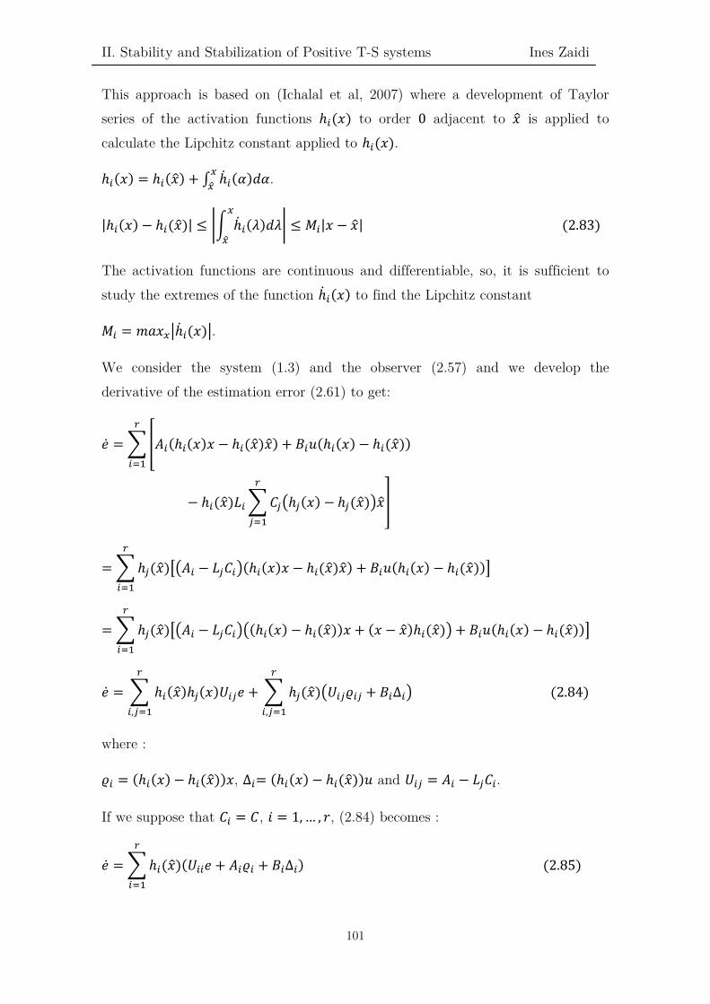
II. Stability and Stabilization of Positive T-S systems Ines Zaidi
This approach is based on (Ichalal et al, 2007) where a development of Taylor series of the activation functions ℎ𝑚𝑚(𝑥𝑥) to order 0 adjacent to 𝑥𝑥� is applied to calculate the Lipchitz constant applied to ℎ𝑚𝑚(𝑥𝑥).
ℎ𝑚𝑚(𝑥𝑥) = ℎ𝑚𝑚(𝑥𝑥�) + ∫ ℎ̇𝑚𝑚(𝛼𝛼)𝑑𝑑𝛼𝛼𝑚𝑚𝑚𝑚� .
|ℎ𝑚𝑚(𝑥𝑥) − ℎ𝑚𝑚(𝑥𝑥�)| ≤ �� ℎ̇𝑚𝑚(𝜆𝜆)𝑑𝑑𝜆𝜆𝑚𝑚
𝑚𝑚�� ≤ 𝑀𝑀𝑚𝑚|𝑥𝑥 − 𝑥𝑥�| (2.83)
The activation functions are continuous and differentiable, so, it is sufficient to study the extremes of the function ℎ̇𝑚𝑚(𝑥𝑥) to find the Lipchitz constant
𝑀𝑀𝑚𝑚 = 𝐼𝐼𝑑𝑑𝑥𝑥𝑚𝑚�ℎ̇𝑚𝑚(𝑥𝑥)�.
We consider the system (1.3) and the observer (2.57) and we develop the derivative of the estimation error (2.61) to get:
�̇�𝑒 = � �𝐴𝐴𝑚𝑚(ℎ𝑚𝑚(𝑥𝑥)𝑥𝑥 − ℎ𝑚𝑚(𝑥𝑥�)𝑥𝑥�) + 𝐵𝐵𝑚𝑚𝑢𝑢(ℎ𝑚𝑚(𝑥𝑥) − ℎ𝑚𝑚(𝑥𝑥�))𝑟𝑟
𝑚𝑚=1
− ℎ𝑚𝑚(𝑥𝑥�)𝐿𝐿𝑚𝑚 � 𝐶𝐶𝑖𝑖�ℎ𝑖𝑖(𝑥𝑥) − ℎ𝑖𝑖(𝑥𝑥�)�𝑥𝑥�𝑟𝑟
𝑖𝑖=1
�
= � ℎ𝑖𝑖(𝑥𝑥�)��𝐴𝐴𝑚𝑚 − 𝐿𝐿𝑖𝑖𝐶𝐶𝑚𝑚�(ℎ𝑚𝑚(𝑥𝑥)𝑥𝑥 − ℎ𝑚𝑚(𝑥𝑥�)𝑥𝑥�) + 𝐵𝐵𝑚𝑚𝑢𝑢(ℎ𝑚𝑚(𝑥𝑥) − ℎ𝑚𝑚(𝑥𝑥�))�𝑟𝑟
𝑚𝑚=1
= � ℎ𝑖𝑖(𝑥𝑥�)��𝐴𝐴𝑚𝑚 − 𝐿𝐿𝑖𝑖𝐶𝐶𝑚𝑚��(ℎ𝑚𝑚(𝑥𝑥) − ℎ𝑚𝑚(𝑥𝑥�))𝑥𝑥 + (𝑥𝑥 − 𝑥𝑥�)ℎ𝑚𝑚(𝑥𝑥�)� + 𝐵𝐵𝑚𝑚𝑢𝑢(ℎ𝑚𝑚(𝑥𝑥) − ℎ𝑚𝑚(𝑥𝑥�))�𝑟𝑟
𝑚𝑚=1
�̇�𝑒 = � ℎ𝑚𝑚(𝑥𝑥�)ℎ𝑖𝑖(𝑥𝑥)𝑈𝑈𝑚𝑚𝑖𝑖𝑒𝑒 + � ℎ𝑖𝑖(𝑥𝑥�)�𝑈𝑈𝑚𝑚𝑖𝑖𝜚𝜚𝑚𝑚𝑖𝑖 + 𝐵𝐵𝑚𝑚∆𝑚𝑚�𝑟𝑟
𝑚𝑚,𝑖𝑖=1
𝑟𝑟
𝑚𝑚,𝑖𝑖=1
(2.84)
where :
𝜚𝜚𝑚𝑚 = (ℎ𝑚𝑚(𝑥𝑥) − ℎ𝑚𝑚(𝑥𝑥�))𝑥𝑥, ∆𝑚𝑚= (ℎ𝑚𝑚(𝑥𝑥) − ℎ𝑚𝑚(𝑥𝑥�))𝑢𝑢 and 𝑈𝑈𝑚𝑚𝑖𝑖 = 𝐴𝐴𝑚𝑚 − 𝐿𝐿𝑖𝑖𝐶𝐶𝑚𝑚.
If we suppose that 𝐶𝐶𝑚𝑚 = 𝐶𝐶, 𝑖𝑖 = 1, … , 𝑟𝑟, (2.84) becomes :
�̇�𝑒 = � ℎ𝑚𝑚(𝑥𝑥�)(𝑈𝑈𝑚𝑚𝑚𝑚𝑒𝑒 + 𝐴𝐴𝑚𝑚𝜚𝜚𝑚𝑚 + 𝐵𝐵𝑚𝑚∆𝑚𝑚)𝑟𝑟
𝑚𝑚=1
(2.85)
101

II. Stability and Stabilization of Positive T-S systems Ines Zaidi
We consider the following hypothesis for the inequality (2.83):
⎩⎪⎨
⎪⎧
‖𝑥𝑥‖ ≤ 𝛽𝛽1 ‖𝑢𝑢‖ ≤ 𝛽𝛽2 ‖ℎ𝑚𝑚(𝑥𝑥) − ℎ𝑚𝑚(𝑥𝑥�)‖
�𝜚𝜚𝑚𝑚𝑖𝑖� ≤ 𝑀𝑀𝑚𝑚𝛽𝛽1‖𝑒𝑒‖‖∆𝑚𝑚‖ ≤ 𝑀𝑀𝑚𝑚𝛽𝛽2‖𝑒𝑒‖
≤ 𝑀𝑀𝑚𝑚‖𝑥𝑥 − 𝑥𝑥�‖ (2.86)
where 𝑀𝑀𝑚𝑚 is the constant of Lipchitz and 𝛽𝛽1 and 𝛽𝛽2 are positive scalars.
With these assumptions, the conditions for the convergence of the error described by (2.84) are given in the following theorem:
Theorem 2.13. (Zaidi et al.)
The estimation error system in (2.84) is positive and globally asymptotically converges to zero if there is a symmetric matrix 𝑃𝑃 > 0, a symmetric matrix
𝑄𝑄 ≥ 0, matrices 𝐹𝐹𝑚𝑚, 𝑖𝑖 = 1, … , 𝑟𝑟 and positive scalars 𝜉𝜉, 𝜆𝜆1 and 𝜆𝜆2 such that:
⎩⎪⎪⎪⎪⎨
⎪⎪⎪⎪⎧
𝑃𝑃 > 0, 𝑄𝑄 ≥ 0, 𝜆𝜆1 > 0, 𝜆𝜆2 > 0, 𝛾𝛾1 > 0, 𝛾𝛾2 > 0 𝐴𝐴𝑚𝑚
𝑇𝑇𝑃𝑃 + 𝑃𝑃𝐴𝐴𝑚𝑚 − 𝐶𝐶𝑚𝑚𝑇𝑇𝐹𝐹𝑚𝑚 − 𝐹𝐹𝑚𝑚𝐶𝐶𝑚𝑚 < −𝑄𝑄, 𝑖𝑖 = 1, … , 𝑟𝑟
�𝐴𝐴𝑚𝑚 + 𝐴𝐴𝑖𝑖
2�
𝑇𝑇
𝑃𝑃 + 𝑃𝑃 �𝐴𝐴𝑚𝑚 + 𝐴𝐴𝑖𝑖
2� −
𝐶𝐶𝑖𝑖𝑇𝑇𝐹𝐹𝑚𝑚 + 𝐹𝐹𝑚𝑚𝐶𝐶𝑖𝑖
2−
𝐶𝐶𝑚𝑚𝑇𝑇𝐹𝐹𝑖𝑖 + 𝐹𝐹𝑖𝑖𝐶𝐶𝑚𝑚
2≤ −𝑄𝑄, 1 ≤ 𝑖𝑖 < 𝑗𝑗 ≤ 𝑟𝑟
⎝
⎜⎛−
𝑄𝑄𝑟𝑟
+ 𝑀𝑀𝑚𝑚2(𝛾𝛾1 + 𝛾𝛾2)𝐼𝐼 ∗ ∗
𝐴𝐴𝑚𝑚𝑇𝑇𝑃𝑃 − 𝐶𝐶𝑚𝑚
𝑇𝑇𝐹𝐹𝑖𝑖𝑇𝑇 −𝜆𝜆1𝐼𝐼 0
𝐵𝐵𝑚𝑚𝑇𝑇𝑃𝑃 0 −𝜆𝜆2𝐼𝐼⎠
⎟⎞
, 𝑖𝑖, 𝑗𝑗 = 1, … , 𝑟𝑟
𝑃𝑃𝐴𝐴𝑚𝑚 − 𝐹𝐹𝑚𝑚𝐶𝐶𝑚𝑚 + 𝜉𝜉𝑃𝑃 ≽ 0
(2.87)
where:
𝛾𝛾1 = 𝜆𝜆1𝛽𝛽12, 𝛾𝛾2 = 𝜆𝜆2𝛽𝛽2
2 and 𝐹𝐹𝑚𝑚 = 𝑃𝑃𝐿𝐿𝑚𝑚 , 𝑖𝑖 = 1, … , 𝑟𝑟 are the observer gains.
Remark 2.7.
when 𝐶𝐶𝑚𝑚 = 𝐶𝐶, 𝑖𝑖 = 1, … , 𝑟𝑟, we get the following result:
102

II. Stability and Stabilization of Positive T-S systems Ines Zaidi
⎩⎪⎪⎪⎨
⎪⎪⎪⎧
𝑃𝑃 > 0, 𝑄𝑄 ≥ 0, 𝜆𝜆1 > 0, 𝜆𝜆2 > 0, 𝛾𝛾1 > 0, 𝛾𝛾2 > 0 𝐴𝐴𝑚𝑚
𝑇𝑇𝑃𝑃 + 𝑃𝑃𝐴𝐴𝑚𝑚 − 𝐶𝐶𝐹𝐹𝑚𝑚 − 𝐹𝐹𝑚𝑚𝐶𝐶 < −𝑄𝑄, 𝑖𝑖 = 1, … , 𝑟𝑟
⎝
⎜⎛−
𝑄𝑄𝑟𝑟
+ 𝑀𝑀𝑚𝑚2(𝛾𝛾1 + 𝛾𝛾2)𝐼𝐼 ∗ ∗
𝐴𝐴𝑚𝑚𝑇𝑇𝑃𝑃 − 𝐶𝐶𝑚𝑚
𝑇𝑇𝐹𝐹𝑖𝑖𝑇𝑇 −𝜆𝜆1𝐼𝐼 0
𝐵𝐵𝑚𝑚𝑇𝑇𝑃𝑃 0 −𝜆𝜆2𝐼𝐼⎠
⎟⎞
, 𝑖𝑖, 𝑗𝑗 = 1, … , 𝑟𝑟
𝑃𝑃𝐴𝐴𝑚𝑚 − 𝐹𝐹𝑚𝑚𝐶𝐶𝑚𝑚 + 𝜉𝜉𝑃𝑃 ≽ 0 𝐵𝐵𝑚𝑚 ≽ 0
(2.88)
Proof:
We consider the Lyapunov function (2.69) applied to the system (2.84) and we develop �̇�𝑉(𝑒𝑒) to obtain:
�̇�𝑉(𝑒𝑒) = � ℎ𝑚𝑚(𝑥𝑥�)ℎ𝑖𝑖(𝑥𝑥�)𝑒𝑒𝑇𝑇�𝑈𝑈𝑚𝑚𝑖𝑖𝑇𝑇 𝑃𝑃 + 𝑃𝑃𝑈𝑈𝑚𝑚𝑖𝑖�𝑒𝑒
𝑟𝑟
𝑚𝑚,𝑖𝑖=1
+ � ℎ𝑖𝑖(𝑥𝑥�)𝑟𝑟
𝑚𝑚,𝑖𝑖=1
�𝜚𝜚𝑚𝑚𝑇𝑇𝑈𝑈𝑚𝑚𝑖𝑖
𝑇𝑇 𝑃𝑃𝑒𝑒 + 𝑒𝑒𝑇𝑇𝑃𝑃𝑈𝑈𝑚𝑚𝑖𝑖𝜚𝜚𝑚𝑚 + ∆𝑚𝑚𝑇𝑇𝐵𝐵𝑚𝑚
𝑇𝑇𝑃𝑃𝑒𝑒 + 𝑒𝑒𝑇𝑇𝑃𝑃𝐵𝐵𝑚𝑚∆𝑚𝑚� (2.89)
Using Lemma B.2 (Annex) and the hypothesis (2.86), we can write:
𝜚𝜚𝑚𝑚𝑇𝑇𝑈𝑈𝑚𝑚𝑖𝑖
𝑇𝑇 𝑃𝑃𝑒𝑒 + 𝑒𝑒𝑇𝑇𝑃𝑃𝑈𝑈𝑚𝑚𝑖𝑖𝜚𝜚𝑚𝑚 ≤ 𝜆𝜆1𝜚𝜚𝑚𝑚𝑇𝑇𝜚𝜚𝑚𝑚 + 𝜆𝜆1
−1𝑒𝑒𝑇𝑇𝑃𝑃𝑈𝑈𝑚𝑚𝑖𝑖𝑈𝑈𝑚𝑚𝑖𝑖𝑇𝑇 𝑃𝑃𝑒𝑒 ≤ 𝜆𝜆1𝑀𝑀𝑚𝑚
2𝛽𝛽12𝑒𝑒𝑇𝑇𝑒𝑒 + 𝜆𝜆1
−1𝑒𝑒𝑇𝑇𝑃𝑃𝑈𝑈𝑚𝑚𝑖𝑖𝑈𝑈𝑚𝑚𝑖𝑖𝑇𝑇 𝑃𝑃𝑒𝑒
(2.90)
∆𝑚𝑚𝑇𝑇𝐵𝐵𝑚𝑚
𝑇𝑇𝑃𝑃𝑒𝑒 + 𝑒𝑒𝑇𝑇𝑃𝑃𝐵𝐵𝑚𝑚∆𝑚𝑚≤ 𝜆𝜆2∆𝑚𝑚𝑇𝑇∆𝑚𝑚 + 𝜆𝜆2
−1𝑒𝑒𝑇𝑇𝑃𝑃𝐵𝐵𝑚𝑚𝐵𝐵𝑚𝑚𝑇𝑇𝑃𝑃𝑒𝑒 ≤ 𝜆𝜆2𝑀𝑀𝑚𝑚
2𝛽𝛽22𝑒𝑒𝑇𝑇𝑒𝑒 + 𝜆𝜆2
−1𝑒𝑒𝑇𝑇𝑃𝑃𝐵𝐵𝑚𝑚𝐵𝐵𝑚𝑚𝑇𝑇𝑃𝑃𝑒𝑒
(2.91)
with 𝜆𝜆1 and 𝜆𝜆2 positive reals.
Thus, the conditions (2.89) can be written as follows:
�̇�𝑉(𝑒𝑒) ≤ � ℎ𝑚𝑚(𝑥𝑥�)ℎ𝑖𝑖(𝑥𝑥�)𝑒𝑒𝑇𝑇�𝑈𝑈𝑚𝑚𝑖𝑖𝑇𝑇 𝑃𝑃 + 𝑃𝑃𝑈𝑈𝑚𝑚𝑖𝑖�𝑒𝑒
𝑟𝑟
𝑚𝑚,𝑖𝑖=1
+ � ℎ𝑖𝑖(𝑥𝑥�)𝑟𝑟
𝑚𝑚,𝑖𝑖=1
𝑒𝑒𝑇𝑇�𝑀𝑀𝑚𝑚2(𝜆𝜆1𝛽𝛽1
2 + 𝜆𝜆2𝛽𝛽22)𝐼𝐼 + 𝜆𝜆1
−1𝑃𝑃𝑈𝑈𝑚𝑚𝑖𝑖𝑈𝑈𝑚𝑚𝑖𝑖𝑇𝑇 𝑃𝑃 + 𝜆𝜆2
−1𝑃𝑃𝐵𝐵𝑚𝑚𝐵𝐵𝑚𝑚𝑇𝑇𝑃𝑃�𝑒𝑒 (2.92)
We suppose that there exists a symmetric matrix 𝑃𝑃 > 0 and a symmetric matrix 𝑄𝑄 ≥ 0 such that:
103

II. Stability and Stabilization of Positive T-S systems Ines Zaidi
� ℎ𝑚𝑚(𝑥𝑥�)ℎ𝑖𝑖(𝑥𝑥�)�𝑈𝑈𝑚𝑚𝑖𝑖𝑇𝑇 𝑃𝑃 + 𝑃𝑃𝑈𝑈𝑚𝑚𝑖𝑖� < −𝑄𝑄
𝑟𝑟
𝑚𝑚,𝑖𝑖=1
(2.93)
Using the results of (Tanaka et al, 1998), condition (2.93) is fulfilled, if there exist matrices 𝑃𝑃 and 𝑄𝑄 such that:
�𝑈𝑈𝑚𝑚𝑚𝑚
𝑇𝑇𝑃𝑃 + 𝑃𝑃𝑈𝑈𝑚𝑚𝑚𝑚 < −𝑄𝑄, 𝑖𝑖 = 1, … , 𝑟𝑟
�𝑈𝑈𝑚𝑚𝑖𝑖 + 𝑈𝑈𝑖𝑖𝑚𝑚�𝑇𝑇
𝑃𝑃 + 𝑃𝑃�𝑈𝑈𝑚𝑚𝑖𝑖 + 𝑈𝑈𝑖𝑖𝑚𝑚� ≤ −2𝑄𝑄, 1 ≤ 𝑖𝑖 < 𝑗𝑗 ≤ 𝑟𝑟 (2.94)
Substituting (2.94) in (2.92), we get:
�̇�𝑉(𝑒𝑒) ≤ � ℎ𝑖𝑖(𝑥𝑥�)𝑟𝑟
𝑚𝑚,𝑖𝑖=1
𝑒𝑒𝑇𝑇 �−𝑄𝑄𝑟𝑟
+ 𝑀𝑀𝑚𝑚2(𝜆𝜆1𝛽𝛽1
2 + 𝜆𝜆2𝛽𝛽22)𝐼𝐼 + 𝜆𝜆1
−1𝑃𝑃𝑈𝑈𝑚𝑚𝑖𝑖𝑈𝑈𝑚𝑚𝑖𝑖𝑇𝑇 𝑃𝑃 + 𝜆𝜆2
−1𝑃𝑃𝐵𝐵𝑚𝑚𝐵𝐵𝑚𝑚𝑇𝑇𝑃𝑃� 𝑒𝑒
(2.95)
To guarantee �̇�𝑉(𝑒𝑒) < 0, it suffices that (2.94) and the following condition hold:
−𝑄𝑄𝑟𝑟
+ 𝑀𝑀𝑚𝑚2(𝜆𝜆1𝛽𝛽1
2 + 𝜆𝜆2𝛽𝛽22)𝐼𝐼 + 𝜆𝜆1
−1𝑃𝑃𝑈𝑈𝑚𝑚𝑖𝑖𝑈𝑈𝑚𝑚𝑖𝑖𝑇𝑇 𝑃𝑃 + 𝜆𝜆2
−1𝑃𝑃𝐵𝐵𝑚𝑚𝐵𝐵𝑚𝑚𝑇𝑇𝑃𝑃 < 0 (2.96)
is verified.
Using (2.94) and the Schur complement (2.96), we get the following conditions:
⎩⎪⎪⎨
⎪⎪⎧
𝑃𝑃 > 0, 𝑄𝑄 ≥ 0, 𝜆𝜆1 > 0, 𝜆𝜆2 > 0, 𝛾𝛾1 > 0, 𝛾𝛾2 > 0 𝑈𝑈𝑚𝑚𝑚𝑚
𝑇𝑇𝑃𝑃 + 𝑃𝑃𝑈𝑈𝑚𝑚𝑚𝑚 < −𝑄𝑄; 𝑖𝑖 = 1, … , 𝑟𝑟
�𝑈𝑈𝑚𝑚𝑖𝑖 + 𝑈𝑈𝑖𝑖𝑚𝑚�𝑇𝑇
𝑃𝑃 + 𝑃𝑃�𝑈𝑈𝑚𝑚𝑖𝑖 + 𝑈𝑈𝑖𝑖𝑚𝑚� ≤ −2𝑄𝑄; 1 ≤ 𝑖𝑖 < 𝑗𝑗 ≤ 𝑟𝑟
⎝
⎛−
𝑄𝑄𝑟𝑟
+ 𝑀𝑀𝑚𝑚2(𝜆𝜆1𝛽𝛽1
2 + 𝜆𝜆2𝛽𝛽22)𝐼𝐼 ∗ ∗
𝑈𝑈𝑚𝑚𝑚𝑚𝑇𝑇𝑃𝑃 −𝜆𝜆1𝑃𝑃 0
𝐵𝐵𝑚𝑚𝑇𝑇𝑃𝑃 0 −𝜆𝜆2𝑃𝑃⎠
⎞ < 0; 𝑖𝑖, 𝑗𝑗 = 1, … , 𝑟𝑟
(2.97)
Replacing 𝑈𝑈𝑚𝑚𝑖𝑖 by 𝐴𝐴𝑚𝑚 − 𝐿𝐿𝑖𝑖𝐶𝐶𝑚𝑚 , conditions (2.97) become:
⎩⎪⎪⎪⎨
⎪⎪⎪⎧
𝑃𝑃 > 0, 𝑄𝑄 ≥ 0, 𝜆𝜆1 > 0, 𝜆𝜆2 > 0, 𝛾𝛾1 > 0, 𝛾𝛾2 > 0 𝐴𝐴𝑚𝑚
𝑇𝑇𝑃𝑃 + 𝑃𝑃𝐴𝐴𝑚𝑚 − 𝐶𝐶𝑚𝑚𝑇𝑇𝐿𝐿𝑚𝑚
𝑇𝑇𝑃𝑃 − 𝑃𝑃𝐿𝐿𝑚𝑚𝐶𝐶𝑚𝑚 < −𝑄𝑄; 𝑖𝑖 = 1, … , 𝑟𝑟
�𝐴𝐴𝑚𝑚 + 𝐴𝐴𝑖𝑖�𝑇𝑇
𝑃𝑃 + 𝑃𝑃�𝐴𝐴𝑚𝑚 + 𝐴𝐴𝑖𝑖� − 𝐶𝐶𝑖𝑖𝑇𝑇𝐿𝐿𝑚𝑚
𝑇𝑇𝑃𝑃 − 𝑃𝑃𝐿𝐿𝑚𝑚𝐶𝐶𝑖𝑖 − 𝐶𝐶𝑚𝑚𝑇𝑇𝐿𝐿𝑖𝑖
𝑇𝑇𝑃𝑃 − 𝑃𝑃𝐿𝐿𝑖𝑖𝐶𝐶𝑚𝑚 ≤ −2𝑄𝑄; 1 ≤ 𝑖𝑖 < 𝑗𝑗 ≤ 𝑟𝑟
⎝
⎛−
𝑄𝑄𝑟𝑟
+ 𝑀𝑀𝑚𝑚2(𝜆𝜆1𝛽𝛽1
2 + 𝜆𝜆2𝛽𝛽22)𝐼𝐼 ∗ ∗
𝑈𝑈𝑚𝑚𝑚𝑚𝑇𝑇𝑃𝑃 −𝜆𝜆1𝑃𝑃 0
𝐵𝐵𝑚𝑚𝑇𝑇𝑃𝑃 0 −𝜆𝜆2𝑃𝑃⎠
⎞ < 0; 𝑖𝑖, 𝑗𝑗 = 1, … , 𝑟𝑟
(2.98)
104
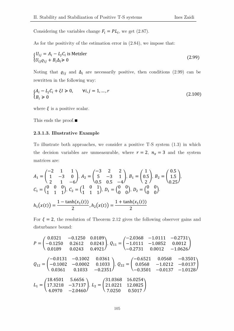
II. Stability and Stabilization of Positive T-S systems Ines Zaidi
Considering the variables change 𝐹𝐹𝑚𝑚 = 𝑃𝑃𝐿𝐿𝑚𝑚, we get (2.87).
As for the positivity of the estimation error in (2.84), we impose that:
�𝑈𝑈𝑚𝑚𝑖𝑖 = 𝐴𝐴𝑚𝑚 − 𝐿𝐿𝑖𝑖𝐶𝐶𝑚𝑚 is Metzler 𝑈𝑈𝑚𝑚𝑖𝑖𝜚𝜚𝑚𝑚𝑖𝑖 + 𝐵𝐵𝑚𝑚∆𝑚𝑚≽ 0 (2.99)
Noting that 𝜚𝜚𝑚𝑚𝑖𝑖 and ∆𝑚𝑚 are necessarily positive, then conditions (2.99) can be
rewritten in the following way:
�𝐴𝐴𝑚𝑚 − 𝐿𝐿𝑖𝑖𝐶𝐶𝑚𝑚 + 𝜉𝜉𝐼𝐼 ≽ 0, ∀𝑖𝑖, 𝑗𝑗 = 1, … , 𝑟𝑟𝐵𝐵𝑚𝑚 ≽ 0 (2.100)
where 𝜉𝜉 is a positive scalar.
This ends the proof.∎
2.3.1.3. Illustrative Example
To illustrate both approaches, we consider a positive T-S system (1.3) in which the decision variables are unmeasurable, where 𝑟𝑟 = 2, 𝑛𝑛𝑚𝑚 = 3 and the system matrices are:
𝐴𝐴1 = �−2 1 11 −3 02 1 −6
�, 𝐴𝐴2 = �−3 2 25 −3 1
0.5 0.5 −4�, 𝐵𝐵1 = �
10.52
�, 𝐵𝐵2 = �0.51.5
0.25�,
𝐶𝐶1 = �0 0 01 1 1�, 𝐶𝐶2 = �1 0 1
1 1 1�, 𝐷𝐷1 = �0 00 0�, 𝐷𝐷2 = �0 0
0 0�.
ℎ1�𝑥𝑥(𝑡𝑡)� =1 − tanh (𝑥𝑥1(𝑡𝑡))
2, ℎ2�𝑥𝑥(𝑡𝑡)� =
1 + tanh (𝑥𝑥1(𝑡𝑡))2
For 𝜉𝜉 = 2, the resolution of Theorem 2.12 gives the following observer gains and disturbance bound:
𝑃𝑃 = �0.0321 −0.1250 0.0189
−0.1250 0.2612 0.02430.0189 0.0243 0.4921
�, 𝑄𝑄11 = �−2.0368 −1.0111 −0.2731−1.0111 −1.0852 0.0012−0.2731 0.0012 −1.0626
�
𝑄𝑄12 = �−0.0131 −0.1002 0.0361−0.1002 −0.0002 0.10330.0361 0.1033 −0.2351
�, 𝑄𝑄22 = �−0.6521 0.0568 −0.35010.0568 −1.0212 −0.0137
−0.3501 −0.0137 −1.0128�
𝐿𝐿1 = �18.4501 5.665617.3218 −3.71374.0970 −2.0460
�, 𝐿𝐿2 = �31.0368 16.025421.0221 12.08257.0250 0.5017
�
105

II. Stability and Stabilization of Positive T-S systems Ines Zaidi
𝛼𝛼 = 1.2051, 𝛽𝛽 = 0.6641
When checking the feasibility of Theorem 2.12, we note that for 𝛽𝛽 > 2.7301, the conditions (2.67) do not have solution.
The resolution of Theorem 2.13, with 𝜉𝜉 = 2 and the Lipschitz constants given by: 𝑀𝑀1 = 𝑀𝑀2 = 0.8 yields:
𝑃𝑃 = �1.7292 −3.6620 −0.7908
−3.6620 5.7213 0.1021−0.7908 0.1021 10.7057
�, 𝑄𝑄 = �54.0250 −7.0012 17.9120−7.0012 11.2372 25.321817.9120 25.3218 81.5017
�
𝐿𝐿1 = �21.0368 32.00215.0111 17.69281.7137 8.6665
�, 𝐿𝐿2 = �12.2450 15.91614.9415 12.66202.5621 5.2372
�
𝜆𝜆1 = 126.0421, 𝜆𝜆2 = 25.9043
𝛽𝛽1 = 0.6182, 𝛽𝛽2 = 0.3521
Figures 2.6-2.8 illustrate the state estimation errors of the system for both approaches with the input 𝑢𝑢(𝑡𝑡) in Figure 2.5:
Figure 2. 5. The evolution of the system input 𝑢𝑢(𝑡𝑡)
106

II. Stability and Stabilization of Positive T-S systems Ines Zaidi
Figure 2. 6. The evolution of the state estimation error 𝑒𝑒1(𝑡𝑡)
Figure 2. 7. The evolution of the state estimation error 𝑒𝑒2(𝑡𝑡)
107

II. Stability and Stabilization of Positive T-S systems Ines Zaidi
Figure 2. 8. The evolution of the state estimation error 𝑒𝑒3(𝑡𝑡)
We can note the rapid convergence of the state estimation errors for both approaches. In addition, the errors always remain nonnegative. However, Theorem 2.13 presents a slight better performance in guaranteeing the estimation error convergence.
2.4. Conclusion
In this section, we first proposed quadratic stabilization approaches to design state-feedback controllers for positive T-S systems, using the concept of Parallel Distributed Compensation. We developed generalized and relaxed stabilization conditions for the stability of positive T-S systems. We have also proposed the decomposition of controller gains to stabilize and 𝛼𝛼-stabilize positive interval T-S systems. The results are used to improve the stability conditions and maximize the decay rate of the exponential stabilization of this class of systems.
Then, we developed results for the stabilization of positive T-S systems with unmeasurable decision variables. The first approach is based on a representation of the estimation error in the case when the decision variables are measurable but affected with disturbance. We have shown the limitation of this approach due to the large bounds that this disturbance can take. In the second approach, the
108

II. Stability and Stabilization of Positive T-S systems Ines Zaidi
expression of the estimation error involves the bounds of the state variables vector and the bounds of the input vector. This approach has the drawback that it requires a bound on the state variables vector.
109

III. Observer-Based Control design for Positive Systems Ines Zaidi
110

III. Observer-Based Control design for Positive Systems Ines Zaidi
Chapter III
Observer-Based Control Design for Positive Systems
111

III. Observer-Based Control design for Positive Systems Ines Zaidi
112

III. Observer-Based Control design for Positive Systems Ines Zaidi
3.1. Introduction
In this chapter, we study the simultaneous state estimation and stabilization of positive linear and T-S systems that maybe have interval uncertainties. For this, we present different approaches for positive observer-based control design, giving LMI conditions.
The issue of control and state constraints is also dealt with: the proposed approach is extended to handle component-wise lower and upper bounds on the controls.
3.2. Observation of Linear Positive Systems
The problem of state estimation is important in identification and control design. We can find in literature the stochastic approach (Kalman filter), the 𝐻𝐻∞ filtering theory and the set-membership approach. We can make an overview on some classical observers, such as the Luenberger one and the well-known Kalman filter, have been firstly presented in (Luenberger, 1966), (Kalman, 1960) and (Julien & Uhlmann, 2004).
3.2.1. INTERVAL OBSERVERS APPROACH
3.2.1.1. Interval observer design using upper and lower errors
In the following, we suppose that the only information available about the uncertainties is that they are bounded by known upper and lower values. We will present positive interval observers with bounded errors for positive linear systems. Bounding observers can guarantee bounds on the estimated states (Gouzé et al, 2000), (Alamo et al, 2005). Other interval estimation methods for uncertain systems can be found in (Chen et al, 1997), (Jaulin et al, 2001), (Jaulin et al, 2002). The interval observers developed here can be expressed by pairs of estimators.
We consider the following dynamical system:
�̇�𝑥(𝑡𝑡) = 𝑓𝑓�𝑥𝑥(𝑡𝑡), 𝜇𝜇, 𝑢𝑢(𝑡𝑡)�, 𝑥𝑥(0) = 𝑥𝑥0 (3.1)
where 𝑓𝑓 is a Lipschitz function that depends on unknown parameters 𝜇𝜇.
113

III. Observer-Based Control design for Positive Systems Ines Zaidi
An interval observer of system (3.1) can be expressed using two dynamical systems as follows:
��̇�𝜔(𝑡𝑡) = 𝑑𝑑 �𝜔𝜔(𝑡𝑡), 𝜔𝜔(𝑡𝑡), 𝑥𝑥(𝑡𝑡), 𝜇𝜇, 𝑢𝑢(𝑡𝑡)� , 𝜔𝜔(0) = 𝑥𝑥0
�̇�𝜔(𝑡𝑡) = 𝑑𝑑 �𝜔𝜔(𝑡𝑡), 𝜔𝜔(𝑡𝑡), 𝑥𝑥(𝑡𝑡), 𝜇𝜇, 𝑢𝑢(𝑡𝑡)� , 𝜔𝜔(0) = 𝑥𝑥0 (3.2)
where their initial conditions are such that 𝑥𝑥0 ≼ 𝑥𝑥0 ≼ 𝑥𝑥0.
Definition 3.1. (Bolajraf et al, 2011)
An interval observer (3.2) for system (3.1) is a pair of upper and lower estimator functions �𝜔𝜔(𝑡𝑡), 𝜔𝜔(𝑡𝑡)� of the real state function 𝑥𝑥(𝑡𝑡), that is,
𝜔𝜔(𝑡𝑡) ≼ 𝑥𝑥(𝑡𝑡) ≼ 𝜔𝜔(𝑡𝑡), 𝑡𝑡 ≥ 0 (3.3)
We will need some other definitions for the rest of the investigation part.
Definition 3.2. (Bolajraf et al, 2011)
An interval observer for system (3.1) is said to be convergent towards to a box if
lim𝑡𝑡→∞ �𝜔𝜔(𝑡𝑡) − 𝜔𝜔(𝑡𝑡)� exists or is bounded.
Definition 3.3. (Bolajraf et al, 2011)
An interval observer of system (3.1) is said to be asymptotically convergent if
lim𝑡𝑡→∞ �𝜔𝜔(𝑡𝑡) − 𝜔𝜔(𝑡𝑡)� = 0.
The main goal is now to design interval observers for systems of the form (3.1), where the initial conditions of the system (3.1) are unknown but bounded 𝑥𝑥0 ≼ 𝑥𝑥0 ≼ 𝑥𝑥0. In addition, we suppose that some parameters of the model are
unknown, so the observer has to be robust. The basic idea investigated is to reconstruct the error dynamics �̇�𝑒(𝑡𝑡) = �̇�𝜔(𝑡𝑡) − �̇�𝜔(𝑡𝑡), which is enforced to be
positive by the proposed approach. First of all, we have to ensure that if the initial error fulfills 𝑒𝑒(0) ≽ 0, the error remains nonnegative 𝑒𝑒(𝑡𝑡) ≽ 0, ∀𝑡𝑡. So, we can guarantee nonnegative lower and upper bounds on the estimated states.
We first consider the following system subject to interval uncertainties:
��̇�𝑥(𝑡𝑡) = 𝐴𝐴𝑥𝑥(𝑡𝑡) + 𝐵𝐵𝑢𝑢(𝑡𝑡) 𝑦𝑦(𝑡𝑡) = 𝐶𝐶𝑥𝑥(𝑡𝑡) (3.4)
114

III. Observer-Based Control design for Positive Systems Ines Zaidi
where 𝑥𝑥(𝑡𝑡) ∈ ℝ+𝑛𝑛𝑥𝑥 is the state vector and 𝑦𝑦(𝑡𝑡) ∈ ℝ𝑛𝑛𝑦𝑦 is the output formed by the
measurements. The initial conditions 𝑥𝑥(0) = 𝑥𝑥0 ∈ ℝ+𝑛𝑛𝑥𝑥 are assumed to be
unknown and bounded. We suppose 𝑢𝑢(𝑡𝑡) = 0.
𝑥𝑥0 ≼ 𝑥𝑥(0) ≼ 𝑥𝑥0 (3.5)
The matrix 𝐴𝐴 ∈ ℝ𝑛𝑛𝑥𝑥×𝑛𝑛𝑥𝑥, which is Metzler, and the matrix 𝐶𝐶 ∈ ℝ𝑛𝑛𝑦𝑦×𝑛𝑛𝑥𝑥 are assumed to be unknown, but bounded by known constant matrices 𝐴𝐴, 𝐴𝐴, 𝐶𝐶 and 𝐶𝐶:
𝐴𝐴 ≼ 𝐴𝐴 ≼ 𝐴𝐴, 𝐶𝐶 ≼ 𝐶𝐶 ≼ 𝐶𝐶 (3.6)
Our goal is to obtain an interval observer of system (3.4) that guarantees bounds on the estimated states. A positive interval observer is proposed in (Bolajraf, 2012) with gain matrix decomposed into matrices:
��̇�𝜔 = �𝐴𝐴 − 𝐿𝐿𝐶𝐶 + 𝐺𝐺𝐶𝐶�𝜔𝜔 + (𝐿𝐿 − 𝐺𝐺)𝑦𝑦, 𝜔𝜔(0) = 𝑥𝑥0
�̇�𝜔 = �𝐴𝐴 − 𝐿𝐿𝐶𝐶 + 𝐺𝐺𝐶𝐶�𝜔𝜔 + (𝐿𝐿 − 𝐺𝐺)𝑦𝑦, 𝜔𝜔(0) = 𝑥𝑥0
0 ≼ 𝜔𝜔(𝑡𝑡) ≼ 𝑥𝑥(𝑡𝑡) ≼ 𝜔𝜔(𝑡𝑡) (3.7)
where the gains 𝐿𝐿 and 𝐺𝐺 have to fulfill the additional constraints
⎩⎪⎨
⎪⎧ 𝐿𝐿 ≽ 0
𝐺𝐺 ≽ 0 𝐿𝐿𝐶𝐶 − 𝐺𝐺𝐶𝐶 ≽ 0 𝐴𝐴 − 𝐿𝐿𝐶𝐶 + 𝐺𝐺𝐶𝐶 is Metzler
(3.8)
By fulfilling the conditions in (3.8) on the gains 𝐿𝐿 and 𝐺𝐺 of the pair of dynamical systems in (3.7), we can demonstrate that 𝜔𝜔(𝑡𝑡) ≼ 𝑥𝑥(𝑡𝑡) ≼ 𝜔𝜔(𝑡𝑡).
For this reason, we can establish the lower and upper errors that follow:
�̇�𝑒 = �𝐴𝐴 − 𝐿𝐿𝐶𝐶 + 𝐺𝐺𝐶𝐶�𝑒𝑒 + �𝐴𝐴 − 𝐴𝐴 + 𝐿𝐿�𝐶𝐶 − 𝐶𝐶� + 𝐺𝐺�𝐶𝐶 − 𝐶𝐶�� 𝑥𝑥 (3.9)
�̇�𝑒 = �𝐴𝐴 − 𝐿𝐿𝐶𝐶 + 𝐺𝐺𝐶𝐶�𝑒𝑒 + �𝐴𝐴 − 𝐴𝐴 + 𝐿𝐿�𝐶𝐶 − 𝐶𝐶� + 𝐺𝐺�𝐶𝐶 − 𝐶𝐶�� 𝑥𝑥 (3.10)
These errors must be nonnegative for all initial conditions 𝑒𝑒0 = 𝜔𝜔0 − 𝑥𝑥0 ≽ 0 and 𝑒𝑒0 = 𝑥𝑥0 − 𝜔𝜔0. In addition, note that the nonnegativity of the lower estimate
𝜔𝜔(𝑡𝑡) ≽ 0 is guaranteed from the condition 𝐿𝐿𝐶𝐶 − 𝐺𝐺𝐶𝐶 ≽ 0. To prove this claim, we
can use Theorem 1.17. and the fact that 𝐴𝐴 − 𝐿𝐿𝐶𝐶 + 𝐺𝐺𝐶𝐶 and 𝐴𝐴 − 𝐿𝐿𝐶𝐶 + 𝐺𝐺𝐶𝐶 are
Metzler, combined with �𝐴𝐴 − 𝐴𝐴 + 𝐿𝐿�𝐶𝐶 − 𝐶𝐶� + 𝐺𝐺�𝐶𝐶 − 𝐶𝐶�� 𝑥𝑥 ≽ 0 and �𝐴𝐴 − 𝐴𝐴 +
𝐿𝐿�𝐶𝐶 − 𝐶𝐶� + 𝐺𝐺�𝐶𝐶 − 𝐶𝐶�� 𝑥𝑥 ≼ 0. Also, we can show that the lower estimate of (3.7)
115

III. Observer-Based Control design for Positive Systems Ines Zaidi
is nonnegative since 𝐴𝐴 − 𝐿𝐿𝐶𝐶 + 𝐺𝐺𝐶𝐶 is Metzler and (𝐿𝐿 − 𝐺𝐺)𝐶𝐶 is a nonnegative
matrix for all 𝐶𝐶 such as 𝐶𝐶 ≼ 𝐶𝐶 ≼ 𝐶𝐶, by noticing that if 𝐿𝐿𝐶𝐶 − 𝐺𝐺𝐶𝐶 is nonnegative
then (𝐿𝐿 − 𝐺𝐺)𝐶𝐶 is nonnegative �𝐿𝐿𝐶𝐶 − 𝐺𝐺𝐶𝐶 ≤ (𝐿𝐿 − 𝐺𝐺)𝐶𝐶�.
We propose an approach of interval observers design with bounded errors, based on LMI formulation.
Theorem 3.1. (Zaidi et al, 2015)
Assume that the trajectory of system (3.4) is bounded, that is, 𝑥𝑥(𝑡𝑡) ≼ 𝑥𝑥, ∀𝑡𝑡 ≥ 0, then, there exists a positive interval observer of system (3.4) of the form (3.7) with bounded error, if the following LMI problem, in the variables 𝛽𝛽 ∈ ℝ+,
𝜆𝜆 ∈ ℝ𝑛𝑛𝑥𝑥, 𝑋𝑋, 𝑌𝑌 ∈ ℝ+𝑛𝑛𝑦𝑦×𝑛𝑛𝑥𝑥, is feasible:
⎩⎪⎪⎨
⎪⎪⎧𝐴𝐴
𝑇𝑇𝑑𝑑𝑖𝑖𝑑𝑑𝑑𝑑(𝜆𝜆) + 𝑑𝑑𝑖𝑖𝑑𝑑𝑑𝑑(𝜆𝜆)𝐴𝐴 − 𝐶𝐶𝑇𝑇𝑋𝑋 − 𝑋𝑋𝐶𝐶 + 𝐶𝐶
𝑇𝑇𝑌𝑌 + 𝑌𝑌𝐶𝐶 < 0
𝐶𝐶𝑇𝑇𝑋𝑋 − 𝐶𝐶𝑇𝑇
𝑌𝑌 ≽ 0
𝐴𝐴𝑇𝑇𝑑𝑑𝑖𝑖𝑑𝑑𝑑𝑑(𝜆𝜆) − 𝐶𝐶𝑇𝑇
𝑋𝑋 + 𝐶𝐶𝑇𝑇𝑌𝑌 + 𝛽𝛽𝐼𝐼 ≽ 0 𝜆𝜆 ≻ 0 𝑋𝑋 ≽ 0 𝑌𝑌 ≽ 0
(3.12𝑑𝑑)(3.12𝑏𝑏)(3.12𝑐𝑐)(3.12𝑑𝑑)(3.12𝑒𝑒)(3.12𝑓𝑓)
Moreover, the gain matrices 𝐿𝐿 and 𝐺𝐺 of the interval observer (3.7) are given by:
𝐿𝐿 = 𝑑𝑑𝑖𝑖𝑑𝑑𝑑𝑑(𝜆𝜆)−1𝑋𝑋𝑇𝑇, 𝐺𝐺 = 𝑑𝑑𝑖𝑖𝑑𝑑𝑑𝑑(𝜆𝜆)−1𝑌𝑌𝑇𝑇 (3.13)
where 𝛽𝛽, 𝜆𝜆, 𝑋𝑋 and 𝑌𝑌 are any feasible solution to the LMI problem (3.12).
Proof:
Assume that the conditions (3.12) are verified and define 𝐿𝐿 = 𝑑𝑑𝑖𝑖𝑑𝑑𝑑𝑑(𝜆𝜆)−1𝑋𝑋𝑇𝑇 and 𝐺𝐺 = 𝑑𝑑𝑖𝑖𝑑𝑑𝑑𝑑(𝜆𝜆)−1𝑌𝑌𝑇𝑇. By simple manipulations, (3.12) is equivalent to
⎩⎪⎪⎪⎨
⎪⎪⎪⎧�𝐴𝐴
𝑇𝑇− 𝐶𝐶𝑇𝑇𝐿𝐿𝑇𝑇 + 𝐶𝐶
𝑇𝑇𝐺𝐺𝑇𝑇� 𝜆𝜆 < 0
𝜆𝜆 ≻ 0 𝐿𝐿𝑇𝑇𝑑𝑑𝑖𝑖𝑑𝑑𝑑𝑑(𝜆𝜆) ≽ 0 𝐺𝐺𝑇𝑇𝑑𝑑𝑖𝑖𝑑𝑑𝑑𝑑(𝜆𝜆) ≽ 0
�𝐶𝐶𝑇𝑇𝐿𝐿𝑇𝑇 − 𝐶𝐶𝑇𝑇
𝐺𝐺𝑇𝑇� 𝑑𝑑𝑖𝑖𝑑𝑑𝑑𝑑(𝜆𝜆) ≽ 0
�𝐴𝐴𝑇𝑇 − 𝐶𝐶𝑇𝑇
𝐿𝐿𝑇𝑇 + 𝐶𝐶𝑇𝑇𝐺𝐺𝑇𝑇� 𝑑𝑑𝑖𝑖𝑑𝑑𝑑𝑑(𝜆𝜆) + 𝛽𝛽𝐼𝐼 ≽ 0
(3.14𝑑𝑑)(3.14𝑏𝑏)(3.14𝑐𝑐)(3.14𝑑𝑑)(3.14𝑒𝑒)(3.14𝑓𝑓)
116

III. Observer-Based Control design for Positive Systems Ines Zaidi
The condition �𝐴𝐴𝑇𝑇 − 𝐶𝐶𝑇𝑇
𝐿𝐿𝑇𝑇 + 𝐶𝐶𝑇𝑇𝐺𝐺𝑇𝑇� 𝑑𝑑𝑖𝑖𝑑𝑑𝑑𝑑(𝜆𝜆) + 𝛽𝛽𝐼𝐼 ≽ 0 equivalently means that
𝐴𝐴𝑇𝑇 − 𝐶𝐶𝑇𝑇
𝐿𝐿𝑇𝑇 + 𝐶𝐶𝑇𝑇𝐺𝐺𝑇𝑇 is Metzler, or equivalently, 𝐴𝐴 − 𝐿𝐿𝐶𝐶 + 𝐺𝐺𝐶𝐶 is Metzler.
The nonnegativity of 𝐿𝐿, 𝐺𝐺 and 𝐿𝐿𝐶𝐶 − 𝐺𝐺𝐶𝐶 are equivalent to the conditions
𝐿𝐿𝑇𝑇𝑑𝑑𝑖𝑖𝑑𝑑𝑑𝑑(𝜆𝜆) ≽ 0, 𝐺𝐺𝑇𝑇𝑑𝑑𝑖𝑖𝑑𝑑𝑑𝑑(𝜆𝜆) ≽ 0 and (𝐶𝐶𝑇𝑇𝐿𝐿𝑇𝑇 − 𝐶𝐶𝑇𝑇
𝐺𝐺𝑇𝑇)𝑑𝑑𝑖𝑖𝑑𝑑𝑑𝑑(𝜆𝜆) ≽ 0. Hence, we know
that the conditions 𝐿𝐿 ≽ 0, 𝐺𝐺 ≽ 0, 𝐿𝐿𝐶𝐶 − 𝐺𝐺𝐶𝐶 ≽ 0 and 𝐴𝐴 − 𝐿𝐿𝐶𝐶 + 𝐺𝐺𝐶𝐶 is Metzler define
a positive interval observer of the form (3.7).
In order to complete the proof, we use the fact that 𝐴𝐴 − 𝐿𝐿𝐶𝐶 + 𝐺𝐺𝐶𝐶 is Hurwitz. To see this, use the fact that 𝐴𝐴 − 𝐿𝐿𝐶𝐶 + 𝐺𝐺𝐶𝐶 is Metzler together with the conditions
�𝐴𝐴𝑇𝑇
− 𝐶𝐶𝑇𝑇𝐿𝐿𝑇𝑇 + 𝐶𝐶𝑇𝑇
𝐺𝐺𝑇𝑇� 𝜆𝜆 ≺ 0, 𝜆𝜆 ≻ 0 and Theorem 1.19.
3.2.1.2. Design of Positive Observers for Interval Systems
We now consider the observer design for the following autonomous positive interval system (3.4), where 𝐴𝐴 ∈ [𝐴𝐴 , 𝐴𝐴] and 𝐶𝐶 ∈ [𝐶𝐶 , 𝐶𝐶] are unknown constant
matrices with known bounds, that fulfill 𝐴𝐴 ∈ ℝ+𝑛𝑛𝑥𝑥×𝑛𝑛𝑥𝑥 is Metzler, 𝐶𝐶 ∈ ℝ+
𝑛𝑛𝑦𝑦×𝑛𝑛𝑥𝑥 and 𝐴𝐴
is Hurwitz (so 𝐴𝐴 is Hurwitz).
Lemma 3.1. (Minc, 1988), (Berman & Plemmons, 1994)
For matrices 𝐴𝐴, 𝐵𝐵 ∈ ℝ𝑛𝑛𝑥𝑥×𝑛𝑛𝑥𝑥, if 𝐵𝐵 is Metzler and 𝐴𝐴 ≽ 𝐵𝐵, then 𝜇𝜇(𝐴𝐴) ≥ 𝜇𝜇(𝐵𝐵).
The more general structure that we will adopt is:
𝑥𝑥�̇(𝑡𝑡) = 𝐺𝐺𝑥𝑥�(𝑡𝑡) + 𝐿𝐿𝑦𝑦(𝑡𝑡) (3.15)
where 𝐺𝐺 ∈ ℝ𝑛𝑛𝑥𝑥×𝑛𝑛𝑥𝑥 and 𝐿𝐿 ∈ ℝ𝑛𝑛𝑥𝑥×𝑛𝑛𝑦𝑦 are the observer matrices to be identified. Define the error as 𝑒𝑒(𝑡𝑡) = 𝑥𝑥(𝑡𝑡) − 𝑥𝑥�(𝑡𝑡), then, the augmented system is given by:
��̇�𝑥(𝑡𝑡)�̇�𝑒(𝑡𝑡)
� = � 𝐴𝐴 0𝐴𝐴 − 𝐿𝐿𝐶𝐶 − 𝐺𝐺 𝐺𝐺� �
𝑥𝑥(𝑡𝑡)𝑒𝑒(𝑡𝑡)
� (3.16)
For positive linear systems, we want also to guarantee the nonnegativity of the estimated state 𝑥𝑥�(𝑡𝑡). Then, referring to Lemma 2.1, it is natural to require that 𝐺𝐺 is Metzler and 𝐿𝐿 ≽ 0. In addition, as seen from (Hof, 1998), the induced error dynamic system is nonnegative for the Luenberger observer. In fact, the nonnegativity of the error 𝑒𝑒(𝑡𝑡) is compulsory for the design of positive interval observers. Therefore, our problem is to design a Metzler 𝐺𝐺 and 𝐿𝐿 ≽ 0 of the
117

III. Observer-Based Control design for Positive Systems Ines Zaidi
positive observer (3.15) such that the augmented system (3.16) is positive and asymptotically stable for any 𝐴𝐴 ∈ [𝐴𝐴, 𝐴𝐴] and 𝐶𝐶 ∈ [𝐶𝐶, 𝐶𝐶].
Remark 3.2.
The positivity specification on the error 𝑒𝑒(𝑡𝑡) facilitates the synthesis of the desired positive observer, but may cause some conservatism.
Necessary and sufficient conditions for the existence of a robust interval observer for positive linear systems are summarized in the following theorem.
Theorem 3.2. (Shu et al, 2008)
There exists a positive observer of the form (3.15) for system (3.16) if and only if there exist matrices 𝑃𝑃 = 𝑑𝑑𝑖𝑖𝑑𝑑𝑑𝑑(𝑝𝑝11, … , 𝑝𝑝𝑛𝑛𝑛𝑛) > 0, 𝑄𝑄 = 𝑑𝑑𝑖𝑖𝑑𝑑𝑑𝑑(𝑞𝑞11, … , 𝑞𝑞𝑛𝑛𝑛𝑛) > 0, 𝑉𝑉 ≽ 0 and Metzler 𝑊𝑊 such that the following LMIs hold:
� 𝑃𝑃𝐴𝐴 + 𝐴𝐴𝑇𝑇
𝑃𝑃 𝐴𝐴𝑇𝑇
𝑄𝑄 − 𝐶𝐶𝑇𝑇𝑉𝑉𝑇𝑇 − 𝑊𝑊𝑇𝑇
𝑄𝑄𝐴𝐴 − 𝑉𝑉𝐶𝐶 − 𝑊𝑊 𝑊𝑊 + 𝑊𝑊𝑇𝑇� < 0 (3.17)
𝑄𝑄𝐴𝐴 − 𝑉𝑉𝐶𝐶 − 𝑊𝑊 ≽ 0 (3.18)
Then, the desired observer matrices can be obtained as follows:
𝐺𝐺 = 𝑄𝑄−1𝑊𝑊, 𝐿𝐿 = 𝑄𝑄−1𝑉𝑉 (3.19)
Based on these results, we propose an approach to synthesize an observer-based state-feedback controller for positive linear systems.
3.2.1.3. Design of Positive Interval Observer-based state-feedback controller
We consider the observer design for the positive interval linear system (3.4), where: 𝑢𝑢(𝑡𝑡) ∈ ℝ𝑛𝑛𝑢𝑢 is the control vector, 𝐴𝐴 ∈ [𝐴𝐴 , 𝐴𝐴], 𝐵𝐵 ∈ [𝐵𝐵 , 𝐵𝐵] and 𝐶𝐶 ∈ [𝐶𝐶 , 𝐶𝐶] are
unknown constant matrices with known bounds, that fulfill: 𝐴𝐴 ∈ ℝ𝑛𝑛𝑥𝑥×𝑛𝑛𝑥𝑥 is
Metzler, 𝐵𝐵 ≽ 0 ∈ ℝ𝑛𝑛𝑥𝑥×𝑛𝑛𝑢𝑢 and 𝐶𝐶 ≽ 0 ∈ ℝ𝑛𝑛𝑦𝑦×𝑛𝑛𝑥𝑥.
Let us suppose the state observer (3.15), which allows the states of the model (3.4) to be estimated.
Consider the state-feedback control given by the following expression:
118

III. Observer-Based Control design for Positive Systems Ines Zaidi
𝑢𝑢(𝑡𝑡) = 𝐾𝐾𝑥𝑥�(𝑡𝑡) (3.20)
where 𝐾𝐾 ∈ ℝ𝑛𝑛𝑦𝑦×𝑛𝑛𝑥𝑥 is the controller matrix to be determined.
Then, the closed-loop system is written as follows:
� �̇�𝑥(𝑡𝑡) = 𝐴𝐴 𝑥𝑥(𝑡𝑡) + 𝐵𝐵 𝐾𝐾𝑥𝑥�(𝑡𝑡) 𝑦𝑦(𝑡𝑡) = 𝐶𝐶 𝑥𝑥(𝑡𝑡) (3.21)
Considering the observer (3.15) and the closed loop system (3.21), we can construct the augmented system as follows:
��̇�𝑥(𝑡𝑡)𝑥𝑥�̇(𝑡𝑡)
� = � 𝐴𝐴 𝐵𝐵𝐾𝐾𝐿𝐿𝐶𝐶 𝐺𝐺 � �
𝑥𝑥(𝑡𝑡)𝑥𝑥�(𝑡𝑡)� (3.22)
Firstly, the aim is to guarantee the asymptotic stability and the positivity of the state 𝑥𝑥(𝑡𝑡). In this context, it is natural to require 𝑥𝑥�(𝑡𝑡) being nonnegative as well. Therefore, the problem is to design 𝐺𝐺, 𝐿𝐿 and 𝐾𝐾 such that the augmented system (3.22) is positive and asymptotically stable. Unfortunately, no feasible solution exists for the LMIs associated to this problem.
To solve this issue, the key lies in the nonnegativity of the error 𝑒𝑒(𝑡𝑡) = 𝑥𝑥(𝑡𝑡) −
𝑥𝑥�(𝑡𝑡). Then, we consider the new augmented system defined by:
��̇�𝑥(𝑡𝑡)�̇�𝑒(𝑡𝑡)
� = � 𝐴𝐴 + 𝐵𝐵𝐾𝐾 −𝐵𝐵𝐾𝐾𝐴𝐴 − 𝐿𝐿𝐶𝐶 + 𝐵𝐵𝐾𝐾 − 𝐺𝐺 𝐺𝐺 − 𝐵𝐵𝐾𝐾� �
𝑥𝑥(𝑡𝑡)𝑒𝑒(𝑡𝑡)� (3.23)
Therefore, the problem is reduced to the determination of the gains 𝐺𝐺, 𝐿𝐿 and 𝐾𝐾 of the augmented system such that the augmented system (3.23) is positive and asymptotically stable. In the following, we provide a necessary condition for the existence of solutions to this problem.
Theorem 3.3. (Zaidi et al, 2014c)
If there exists a static state-feedback controller (3.20) that stabilizes system (3.21), using the observer (3.15), then the following inequalities with respect to Metzler 𝐺𝐺, 𝐿𝐿 ≽ 0 and 𝐾𝐾 ≼ 0 have a solution:
𝑡𝑡𝑟𝑟𝑑𝑑𝑐𝑐𝑒𝑒�𝐴𝐴 + 𝐺𝐺 + (𝐵𝐵 − 𝐵𝐵)𝐾𝐾� < 0 (3.24)
[𝐴𝐴 + 𝐵𝐵𝐾𝐾]𝑚𝑚𝑖𝑖 ≥ 0 , 1 ≤ 𝑖𝑖 ≠ 𝑗𝑗 ≤ 𝑛𝑛 (3.25)
[𝐺𝐺 − 𝐵𝐵𝐾𝐾]𝑚𝑚𝑖𝑖 ≥ 0 , 1 ≤ 𝑖𝑖 ≠ 𝑗𝑗 ≤ 𝑛𝑛 (3.26)
119

III. Observer-Based Control design for Positive Systems Ines Zaidi
𝐴𝐴 − 𝐿𝐿𝐶𝐶 + 𝐵𝐵𝐾𝐾 − 𝐺𝐺 ≽ 0 (3.27)
Proof:
If the augmented system (2.23) is stable and positive we have that, we have that
𝜇𝜇 �� 𝐴𝐴 + 𝐵𝐵𝐾𝐾 −𝐵𝐵𝐾𝐾𝐴𝐴 − 𝐿𝐿𝐶𝐶 + 𝐵𝐵𝐾𝐾 − 𝐺𝐺 𝐺𝐺 − 𝐵𝐵𝐾𝐾�� < 0 (3.28)
� 𝐴𝐴 + 𝐵𝐵𝐾𝐾 −𝐵𝐵𝐾𝐾𝐴𝐴 − 𝐿𝐿𝐶𝐶 + 𝐵𝐵𝐾𝐾 − 𝐺𝐺 𝐺𝐺 − 𝐵𝐵𝐾𝐾� is Metzler (3.29)
As we have that:
�𝐴𝐴 + 𝐵𝐵𝐾𝐾 −𝐵𝐵𝐾𝐾
𝐴𝐴 − 𝐿𝐿𝐶𝐶 + 𝐵𝐵𝐾𝐾 − 𝐺𝐺 𝐺𝐺 − 𝐵𝐵𝐾𝐾� ≼ � 𝐴𝐴 + 𝐵𝐵𝐾𝐾 −𝐵𝐵𝐾𝐾
𝐴𝐴 − 𝐿𝐿𝐶𝐶 + 𝐵𝐵𝐾𝐾 − 𝐺𝐺 𝐺𝐺 − 𝐵𝐵𝐾𝐾�
≼ �𝐴𝐴 + 𝐵𝐵𝐾𝐾 −𝐵𝐵𝐾𝐾
𝐴𝐴 − 𝐿𝐿𝐶𝐶 + 𝐵𝐵𝐾𝐾 − 𝐺𝐺 𝐺𝐺 − 𝐵𝐵𝐾𝐾� (3.30)
Then, we deduce, using (3.28), that
𝜇𝜇 ��𝐴𝐴 + 𝐵𝐵𝐾𝐾 −𝐵𝐵𝐾𝐾
𝐴𝐴 − 𝐿𝐿𝐶𝐶 + 𝐵𝐵𝐾𝐾 − 𝐺𝐺 𝐺𝐺 − 𝐵𝐵𝐾𝐾�� < 0 (3.31)
And using
�𝐴𝐴 + 𝐵𝐵𝐾𝐾 −𝐵𝐵𝐾𝐾
𝐴𝐴 − 𝐿𝐿𝐶𝐶 + 𝐵𝐵𝐾𝐾 − 𝐺𝐺 𝐺𝐺 − 𝐵𝐵𝐾𝐾� is Metzler (3.32)
It follows from (3.31) that
𝑡𝑡𝑟𝑟𝑑𝑑𝑐𝑐𝑒𝑒 ��𝐴𝐴 + 𝐵𝐵𝐾𝐾 −𝐵𝐵𝐾𝐾
𝐴𝐴 − 𝐿𝐿𝐶𝐶 + 𝐵𝐵𝐾𝐾 − 𝐺𝐺 𝐺𝐺 − 𝐵𝐵𝐾𝐾�� < 0 (3.33)
which is equivalent to (3.24). Finally, it is obvious that (3.32) is equivalent to (3.25), (3.26) and (3.27), which completes the proof. ∎
Next, we further study sufficient conditions and the corresponding synthesis approach.
Theorem 3.4. (Zaidi et al, 2014c)
There exists a static state-feedback controller (3.20) that stabilizes system (3.21) using the observer (3.15), if for a positive scalar 𝜀𝜀, there exist matrices
𝑃𝑃 = 𝑑𝑑𝑖𝑖𝑑𝑑𝑑𝑑(𝑃𝑃1, 𝑃𝑃2) > 0, a Metzler matrix 𝐺𝐺, 𝐿𝐿 ≽ 0 and 𝐾𝐾 ≼ 0 such that:
120

III. Observer-Based Control design for Positive Systems Ines Zaidi
�𝒜𝒜𝑇𝑇𝑃𝑃 + 𝑃𝑃𝒜𝒜 − 𝜀𝜀ℬℬ𝑇𝑇𝑃𝑃 − 𝜀𝜀𝑃𝑃ℬ𝑇𝑇ℬ 𝑃𝑃ℬ + 𝒞𝒞𝑇𝑇𝒦𝒦𝑇𝑇
∗ −𝐼𝐼� < 0 (3.34)
[𝐴𝐴 + 𝐵𝐵𝐾𝐾]𝑚𝑚𝑖𝑖 ≥ 0 , 1 ≤ 𝑖𝑖 ≠ 𝑗𝑗 ≤ 𝑛𝑛 (3.35)
[𝐺𝐺 − 𝐵𝐵𝐾𝐾]𝑚𝑚𝑖𝑖 ≥ 0 , 1 ≤ 𝑖𝑖 ≠ 𝑗𝑗 ≤ 𝑛𝑛 (3.36)
𝐴𝐴 − 𝐿𝐿𝐶𝐶 + 𝐵𝐵𝐾𝐾 − 𝐺𝐺 ≽ 0, (3.37) where:
𝒜𝒜 = �𝐴𝐴 0𝐴𝐴 0
� , ℬ = �0 𝐵𝐵 − 𝐵𝐵 0 𝐵𝐵0 𝐵𝐵 − 𝐵𝐵 −𝐼𝐼 𝐵𝐵
�
𝒦𝒦 = �
𝐺𝐺 𝐿𝐿 0 0𝐾𝐾 0 0 00 0 𝐺𝐺 𝐿𝐿0 0 𝐾𝐾 0
�, 𝒞𝒞 = �
0 𝐼𝐼0 0𝐼𝐼 −𝐼𝐼𝐶𝐶 0
� (3.38)
Proof:
It follows from (3.35) that 𝐴𝐴 + 𝐵𝐵𝐾𝐾 is Metzler. Combining this with 𝐾𝐾 ≼ 0 and
𝐿𝐿 ≽ 0 yields that, for any 𝐴𝐴 ∈ [𝐴𝐴, 𝐴𝐴], 𝐵𝐵 ∈ [𝐵𝐵, 𝐵𝐵] and 𝐶𝐶 ∈ [𝐶𝐶, 𝐶𝐶]:
𝐴𝐴 + 𝐵𝐵𝐾𝐾 ≽ 𝐴𝐴 + 𝐵𝐵𝐾𝐾 is Metzler (3.39)
and
𝐴𝐴 − 𝐿𝐿𝐶𝐶 + 𝐵𝐵𝐾𝐾 − 𝐺𝐺 ≽ 𝐴𝐴 − 𝐿𝐿𝐶𝐶 + 𝐵𝐵𝐾𝐾 − 𝐺𝐺 ≽ 0 (3.40)
In addition, from 𝐺𝐺 being Metzler and 𝐾𝐾 ≼ 0 , we obtain that, for any 𝐵𝐵 ∈ [𝐵𝐵, 𝐵𝐵]:
−𝐵𝐵𝐾𝐾 ≽ 0 (3.41)
and
𝐺𝐺 − 𝐵𝐵𝐾𝐾 is Metzler (3.42)
Therefore, from (3.39), (3.40), (3.41) and (3.42), we have that, for any 𝐴𝐴 ∈ [𝐴𝐴, 𝐴𝐴],
𝐵𝐵 ∈ [𝐵𝐵, 𝐵𝐵] and 𝐶𝐶 ∈ [𝐶𝐶, 𝐶𝐶], the augmented system (3.23) is positive.
It follows from (3.34), by the Schur complement, that:
𝒜𝒜𝑇𝑇𝑃𝑃 + 𝑃𝑃𝒜𝒜 − 𝜀𝜀ℬℬ𝑇𝑇𝑃𝑃 − 𝜀𝜀𝑃𝑃ℬ𝑇𝑇ℬ + 𝜀𝜀2ℬℬ𝑇𝑇 + (ℬ𝑇𝑇𝑃𝑃 + 𝒦𝒦 𝒞𝒞)𝑇𝑇(ℬ𝑇𝑇𝑃𝑃 + 𝒦𝒦 𝒞𝒞) ≺ 0 (3.43)
Taking into account the following relationship:
𝑃𝑃𝐵𝐵𝐵𝐵𝑇𝑇𝑃𝑃 − 𝜀𝜀𝐵𝐵𝐵𝐵𝑇𝑇𝑃𝑃 − 𝜀𝜀𝑃𝑃𝐵𝐵𝑇𝑇𝐵𝐵 + 𝜀𝜀2𝐵𝐵𝐵𝐵𝑇𝑇 = (𝑃𝑃𝐵𝐵 − 𝜀𝜀 𝐵𝐵)(𝐵𝐵𝑇𝑇𝑃𝑃 − 𝜀𝜀𝐵𝐵𝑇𝑇) ≥ 0 (3.44)
121

III. Observer-Based Control design for Positive Systems Ines Zaidi
we obtain the following inequality:
𝒜𝒜𝑇𝑇𝑃𝑃 + 𝑃𝑃𝒜𝒜 − 𝑃𝑃ℬℬ𝑇𝑇𝑃𝑃 + (ℬ𝑇𝑇𝑃𝑃 + 𝒦𝒦 𝒞𝒞)𝑇𝑇(ℬ𝑇𝑇𝑃𝑃 + 𝒦𝒦 𝒞𝒞) < 0 (3.45)
Rewriting (3.56) yields that:
(𝒜𝒜 + ℬ𝒦𝒦𝒞𝒞)𝑇𝑇𝑃𝑃 + 𝑃𝑃(𝒜𝒜 + ℬ𝒦𝒦𝒞𝒞) + 𝒞𝒞𝑇𝑇𝒦𝒦𝑇𝑇𝒦𝒦 𝒞𝒞 < 0 (3.46)
which implies that:
(𝒜𝒜 + ℬ𝒦𝒦𝒞𝒞)𝑇𝑇𝑃𝑃 + 𝑃𝑃(𝒜𝒜 + ℬ𝒦𝒦𝒞𝒞) < 0 (3.47)
Therefore, we get:
𝜇𝜇(𝒜𝒜 + ℬ𝒦𝒦𝒞𝒞) < 0 (3.48)
Some algebraic manipulations lead to:
𝒜𝒜 + ℬ𝒦𝒦𝒞𝒞 = �𝐴𝐴 + 𝐵𝐵𝐾𝐾 −𝐵𝐵𝐾𝐾
𝐴𝐴 − 𝐿𝐿𝐶𝐶 + 𝐵𝐵𝐾𝐾 − 𝐺𝐺 𝐺𝐺 − 𝐵𝐵𝐾𝐾� (3.49)
In addition, it is easy to show that:
�𝐴𝐴 + 𝐵𝐵𝐾𝐾 −𝐵𝐵𝐾𝐾
𝐴𝐴 − 𝐿𝐿𝐶𝐶 + 𝐵𝐵𝐾𝐾 − 𝐺𝐺 𝐺𝐺 − 𝐵𝐵𝐾𝐾� ≽ � 𝐴𝐴 + 𝐵𝐵𝐾𝐾 −𝐵𝐵𝐾𝐾
𝐴𝐴 − 𝐿𝐿𝐶𝐶 + 𝐵𝐵𝐾𝐾 − 𝐺𝐺 𝐺𝐺 − 𝐵𝐵𝐾𝐾� (3.50)
Therefore, by combining (3.48)-(3.50) and using Lemma 3.1, we obtain that:
𝜇𝜇 �� 𝐴𝐴 + 𝐵𝐵𝐾𝐾 −𝐵𝐵𝐾𝐾𝐴𝐴 − 𝐿𝐿𝐶𝐶 + 𝐵𝐵𝐾𝐾 − 𝐺𝐺 𝐺𝐺 − 𝐵𝐵𝐾𝐾�� < 0 (3.51)
which means that (3.23) is asymptotically stable for any 𝐴𝐴 ∈ [𝐴𝐴, 𝐴𝐴], 𝐵𝐵 ∈ [𝐵𝐵, 𝐵𝐵]
and 𝐶𝐶 ∈ [𝐶𝐶, 𝐶𝐶], which completes the proof.∎
Remark 3.3.
Using the designed observer-based controller, the state vectors 𝑥𝑥(𝑡𝑡), 𝑥𝑥�(𝑡𝑡) and 𝑒𝑒(𝑡𝑡) will be nonnegative if the initial conditions satisfy 𝑥𝑥(0) ≽ 0 and 𝑥𝑥�(0) ≽ 0. A question which may be asked is why (3.22) is not a positive and asymptotically stable system, even when 𝑥𝑥(𝑡𝑡) and 𝑥𝑥�(𝑡𝑡) are nonnegative and converge to the origin. The reason is that the invariant set associated with (3.22) is not the positive orthant but the cone defined by:
ß = ��𝑥𝑥(𝑡𝑡)𝑥𝑥�(𝑡𝑡)� ≽ 0; [𝐼𝐼 −𝐼𝐼] �
𝑥𝑥(𝑡𝑡)𝑥𝑥�(𝑡𝑡)� ≽ 0�
122

III. Observer-Based Control design for Positive Systems Ines Zaidi
Otherwise, any trajectory of (3.22) starting from [𝑥𝑥𝑇𝑇(0), 𝑥𝑥�𝑇𝑇(0)]𝑇𝑇 ∈ ß will remain in ß for 𝑡𝑡 > 0. If a positive system can be called positive orthant invariant, then the system (3.22) with Metzler 𝐺𝐺, 𝐿𝐿 ≽ 0 and 𝐾𝐾 ≼ 0 obtained through Theorem 3.4 can be viewed as ß invariant. This interpretation may be useful to seek less conservative conditions for such a problem and even to establish solvable necessary and sufficient conditions for the positive stabilization problem with sign-indefinite 𝐾𝐾.
3.2.1.4. Illustrative example
Let us consider the positive interval system (3.4) with:
𝐴𝐴 = �−0.4 0.20.1 −0.5�, 𝐴𝐴 = �−0.2 0.5
0.5 −0.1�,
𝐵𝐵 = �0.30.2� , 𝐵𝐵 = �0.4
0.3�, 𝐶𝐶 = [0.4 0.1] , 𝐶𝐶 = [0.6 0.4].
Then, by using the Scilab 5.3.3 LMI toolbox, it can be seen that the LMIs in Theorems 3.3 and 3.4 are feasible, for 𝜀𝜀 = 15, with the following solution:
𝑃𝑃 = �24.6213 00 12.4880�, 𝐺𝐺 = �−5.2922 0.1028
0.0006 −0.9139�,
𝐾𝐾 = [−1.6628 −1.2478], 𝐿𝐿 = �9.79264.1322�.
Figure 3. 1. Evolution of the state 𝑥𝑥1(𝑡𝑡) and its estimation 𝑥𝑥�1(𝑡𝑡)
123

III. Observer-Based Control design for Positive Systems Ines Zaidi
Figure 3. 2. Evolution of the state 𝑥𝑥2(𝑡𝑡) and its estimation 𝑥𝑥�2(𝑡𝑡)
Figure 3. 3. Evolution of the estimation errors 𝑒𝑒1(𝑡𝑡) and 𝑒𝑒2(𝑡𝑡)
Figures 3.1 to 3.3 show that the evolution of the state vector 𝑥𝑥(𝑡𝑡), as well as its estimated state vector 𝑥𝑥�(𝑡𝑡), remain always nonnegative and converge (the unknown system was simulated for 𝐴𝐴 = 𝐴𝐴, 𝐵𝐵 = 𝐵𝐵, 𝐶𝐶 = 𝐶𝐶). Figures 3.1 and 3.2
illustrate the good estimation and stabilization. Figure 3.3 shows also the nonnegativity of the estimation errors. These facts show the effectiveness of the proposed approach.
3.3. Observer-based Control Design for Positive T-S Systems
124
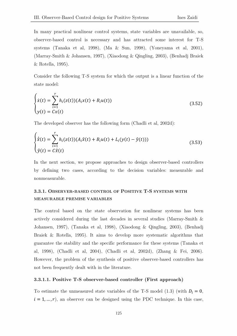
III. Observer-Based Control design for Positive Systems Ines Zaidi
In many practical nonlinear control systems, state variables are unavailable, so, observer-based control is necessary and has attracted some interest for T-S systems (Tanaka et al, 1998), (Ma & Sun, 1998), (Yoneyama et al, 2001), (Marray-Smith & Johansen, 1997), (Xiaodong & Qingling, 2003), (Benhadj Braiek & Rotella, 1995).
Consider the following T-S system for which the output is a linear function of the state model:
��̇�𝑥(𝑡𝑡) = � ℎ𝑚𝑚(𝑧𝑧(𝑡𝑡))(𝐴𝐴𝑚𝑚𝑥𝑥(𝑡𝑡) + 𝐵𝐵𝑚𝑚𝑢𝑢(𝑡𝑡))𝑟𝑟
𝑚𝑚=1𝑦𝑦(𝑡𝑡) = 𝐶𝐶𝑥𝑥(𝑡𝑡)
(3.52)
The developed observer has the following form (Chadli et al, 2002d):
�𝑥𝑥�̇(𝑡𝑡) = � ℎ𝑚𝑚(𝑧𝑧(𝑡𝑡))(𝐴𝐴𝑚𝑚𝑥𝑥�(𝑡𝑡) + 𝐵𝐵𝑚𝑚𝑢𝑢(𝑡𝑡) + 𝐿𝐿𝑚𝑚(𝑦𝑦(𝑡𝑡) − 𝑦𝑦�(𝑡𝑡)))𝑟𝑟
𝑚𝑚=1𝑦𝑦�(𝑡𝑡) = 𝐶𝐶𝑥𝑥�(𝑡𝑡)
(3.53)
In the next section, we propose approaches to design observer-based controllers by defining two cases, according to the decision variables: measurable and nonmeasurable.
3.3.1. OBSERVER-BASED CONTROL OF POSITIVE T-S SYSTEMS WITH
MEASURABLE PREMISE VARIABLES
The control based on the state observation for nonlinear systems has been actively considered during the last decades in several studies (Marray-Smith & Johansen, 1997), (Tanaka et al, 1998), (Xiaodong & Qingling, 2003), (Benhadj Braiek & Rotella, 1995). It aims to develop more systematic algorithms that guarantee the stability and the specific performance for these systems (Tanaka et al, 1998), (Chadli et al, 2004), (Chadli et al, 2002d), (Zhang & Fei, 2006). However, the problem of the synthesis of positive observer-based controllers has not been frequently dealt with in the literature.
3.3.1.1. Positive T-S observer-based controller (First approach)
To estimate the unmeasured state variables of the T-S model (1.3) (with 𝐷𝐷𝑚𝑚 = 0, 𝑖𝑖 = 1, … , 𝑟𝑟), an observer can be designed using the PDC technique. In this case,
125

III. Observer-Based Control design for Positive Systems Ines Zaidi
the overall observer is obtained by linear interpolation of local Luenberger monitors (Luenberger, 1963) associated with different submodels.
The decision variables are supposed measurable, with the T-S system (1.3), locally detectable (i.e, all pairs (𝐴𝐴𝑚𝑚, 𝐶𝐶𝑚𝑚), 𝑖𝑖 = 1, … , 𝑟𝑟 are observable).
We consider the state estimation error 𝑒𝑒(𝑡𝑡) = 𝑥𝑥(𝑡𝑡) − 𝑥𝑥�(𝑡𝑡). Its dynamical model is then:
�̇�𝑒(𝑡𝑡) = � ℎ𝑚𝑚(𝑧𝑧)ℎ𝑖𝑖(𝑧𝑧)𝑆𝑆𝑚𝑚𝑖𝑖𝑒𝑒(𝑡𝑡)𝑟𝑟
𝑚𝑚,𝑖𝑖=1
(3.55)
with 𝑆𝑆𝑚𝑚𝑖𝑖 = 𝐴𝐴𝑚𝑚 − 𝐿𝐿𝑚𝑚𝐶𝐶𝑖𝑖.
Let us consider a PDC control law:
𝑢𝑢(𝑡𝑡) = − � ℎ𝑚𝑚(𝑧𝑧)𝐾𝐾𝑚𝑚𝑥𝑥�(𝑡𝑡)𝑟𝑟
𝑚𝑚=1
(3.56)
From (3.54) and (3.56), we get the following observer:
⎩⎪⎨
⎪⎧𝑥𝑥�̇(𝑡𝑡) = � ℎ𝑚𝑚(𝑧𝑧)ℎ𝑖𝑖(𝑧𝑧)�𝐴𝐴𝑚𝑚 − 𝐵𝐵𝑚𝑚𝐾𝐾𝑖𝑖�𝑥𝑥�(𝑡𝑡) + � ℎ𝑚𝑚(𝑧𝑧)ℎ𝑖𝑖(𝑧𝑧)𝐿𝐿𝑚𝑚𝐶𝐶𝑖𝑖𝑒𝑒(𝑡𝑡)
𝑟𝑟
𝑚𝑚,𝑖𝑖=1
𝑟𝑟
𝑚𝑚,𝑖𝑖=1
𝑦𝑦�(𝑡𝑡) = � ℎ𝑚𝑚(𝑧𝑧)𝐶𝐶𝑚𝑚𝑥𝑥�(𝑡𝑡) 𝑟𝑟
𝑚𝑚=1
(3.57)
By considering the augmented state given by 𝑥𝑥�(𝑡𝑡) = [𝑥𝑥�𝑇𝑇(𝑡𝑡) 𝑒𝑒𝑇𝑇(𝑡𝑡)]𝑇𝑇, we can construct then the following augmented system:
𝑥𝑥�̇(𝑡𝑡) = � ℎ𝑚𝑚(𝑧𝑧)ℎ𝑖𝑖(𝑧𝑧)𝑀𝑀𝑚𝑚𝑖𝑖𝑥𝑥�(𝑡𝑡)𝑟𝑟
𝑚𝑚,𝑖𝑖=1
= � ℎ𝑚𝑚2(𝑧𝑧)𝑀𝑀𝑚𝑚𝑚𝑚𝑥𝑥�(𝑡𝑡)
𝑟𝑟
𝑚𝑚=1
+ 2 � ℎ𝑚𝑚(𝑧𝑧)ℎ𝑖𝑖(𝑧𝑧) �𝑀𝑀𝑚𝑚𝑖𝑖 + 𝑀𝑀𝑖𝑖𝑚𝑚
2� 𝑥𝑥�(𝑡𝑡)
𝑟𝑟
1≤𝑚𝑚<𝑖𝑖
(3.58)
where
𝑀𝑀𝑚𝑚𝑖𝑖 = �𝐴𝐴𝑚𝑚 − 𝐵𝐵𝑚𝑚𝐾𝐾𝑖𝑖 𝐿𝐿𝑚𝑚𝐶𝐶𝑖𝑖
0 𝐴𝐴𝑚𝑚 − 𝐿𝐿𝑚𝑚𝐶𝐶𝑖𝑖� = �
𝐺𝐺𝑚𝑚𝑖𝑖 𝐿𝐿𝑚𝑚𝐶𝐶𝑖𝑖0 𝑆𝑆𝑚𝑚𝑖𝑖
�, 𝑖𝑖, 𝑗𝑗 = 1, … , 𝑟𝑟 (3.59)
We can now apply to (3.58) the results of Section 2.2.1 to guarantee the convergence of the error 𝑒𝑒(𝑡𝑡) and the state estimation 𝑥𝑥�(𝑡𝑡).
126

III. Observer-Based Control design for Positive Systems Ines Zaidi
The following result presents the condition guaranteeing the positive stabilization of the augmented system (3.58).
Theorem 3.5. (Zaidi et al, 2015)
If there exist symmetric matrices 𝑃𝑃1 > 0, 𝑃𝑃2 > 0, 𝑄𝑄1 > 0 and 𝑄𝑄2 > 0, a scalar 𝜀𝜀
such that 12
< 𝜀𝜀 < 1 and scalars 𝛽𝛽1 ≥ 0, 𝛽𝛽2 ≥ 0 and 𝑠𝑠 > 1 such that:
⎩⎪⎪⎪⎪⎨
⎪⎪⎪⎪⎧𝐺𝐺𝑚𝑚𝑚𝑚
𝑇𝑇𝑃𝑃1 + 𝑃𝑃1𝐺𝐺𝑚𝑚𝑚𝑚 + (𝑠𝑠 − 𝜀𝜀)𝑄𝑄1 < 0; 𝑖𝑖 = 1, … , 𝑟𝑟
�𝐺𝐺𝑚𝑚𝑖𝑖 + 𝐺𝐺𝑖𝑖𝑚𝑚
2�
𝑇𝑇
𝑃𝑃1 + 𝑃𝑃1 �𝐺𝐺𝑚𝑚𝑖𝑖 + 𝐺𝐺𝑖𝑖𝑚𝑚
2� − 𝜀𝜀𝑄𝑄1 ≤ 0; 𝑖𝑖 < 𝑗𝑗 = 1, … , 𝑟𝑟
𝑆𝑆𝑚𝑚𝑚𝑚𝑇𝑇𝑃𝑃2 + 𝑃𝑃2𝑆𝑆𝑚𝑚𝑚𝑚 + (𝑠𝑠 − 𝜀𝜀)𝑄𝑄2 < 0; 𝑖𝑖 = 1, … , 𝑟𝑟
�𝑆𝑆𝑚𝑚𝑖𝑖 + 𝑆𝑆𝑖𝑖𝑚𝑚
2�
𝑇𝑇
𝑃𝑃2 + 𝑃𝑃2 �𝑆𝑆𝑚𝑚𝑖𝑖 + 𝑆𝑆𝑖𝑖𝑚𝑚
2� − 𝜀𝜀𝑄𝑄2 ≤ 0; 𝑖𝑖 < 𝑗𝑗 = 1, … , 𝑟𝑟
𝑃𝑃1�𝐺𝐺𝑚𝑚𝑖𝑖 + 𝛽𝛽1𝐼𝐼� ≽ 0 𝑃𝑃2�𝑆𝑆𝑚𝑚𝑖𝑖 + 𝛽𝛽2𝐼𝐼� ≽ 0 𝐿𝐿𝑚𝑚𝐶𝐶𝑖𝑖 ≽ 0 ℎ𝑚𝑚�𝑧𝑧(𝑡𝑡)�ℎ𝑖𝑖�𝑧𝑧(𝑡𝑡)� ≠ 0, ∀(𝑖𝑖, 𝑗𝑗),
(3.60)
where: 𝐺𝐺𝑚𝑚𝑖𝑖 = 𝐴𝐴𝑚𝑚 − 𝐵𝐵𝑚𝑚𝐾𝐾𝑖𝑖 and 𝑆𝑆𝑚𝑚𝑖𝑖 = 𝐴𝐴𝑚𝑚 − 𝐿𝐿𝑚𝑚𝐶𝐶𝑖𝑖 (3.61)
Then, the augmented system (3.58) is positive and globally exponentially stable.
Proof :
Consider the following Lyapunov function: 𝑉𝑉(𝑥𝑥) ≐ 𝑥𝑥�𝑇𝑇𝑃𝑃(𝛿𝛿)𝑥𝑥�; 𝑃𝑃(𝛿𝛿) = �𝑃𝑃1 00 𝛿𝛿𝑃𝑃2
�.
Applying Theorem 2.4 for the system (3.58), in order to have �̇�𝑉 < 0, the following inequalities must hold :
𝑀𝑀𝑚𝑚𝑚𝑚𝑇𝑇𝑃𝑃 + 𝑃𝑃𝑀𝑀𝑚𝑚𝑚𝑚 + (𝑠𝑠 − 𝜀𝜀)𝑄𝑄 < 0, 𝑖𝑖 = 1, … , 𝑟𝑟 (3.62𝑑𝑑)
�𝑀𝑀𝑚𝑚𝑖𝑖 + 𝑀𝑀𝑖𝑖𝑚𝑚
2�
𝑇𝑇
𝑃𝑃 + 𝑃𝑃 �𝑀𝑀𝑚𝑚𝑖𝑖 + 𝑀𝑀𝑖𝑖𝑚𝑚
2� − 𝜀𝜀𝑄𝑄 ≤ 0, 𝑖𝑖 < 𝑗𝑗 = 1, … , 𝑟𝑟 (3.62𝑏𝑏)
Replacing 𝑀𝑀𝑚𝑚𝑖𝑖, 𝑃𝑃 and 𝑄𝑄 by their expressions, we get :
�𝐺𝐺𝑚𝑚𝑚𝑚
𝑇𝑇𝑃𝑃1 + 𝑃𝑃1𝐺𝐺𝑚𝑚𝑚𝑚 + (𝑠𝑠 − 𝜀𝜀)𝑄𝑄1 𝑃𝑃1𝐿𝐿𝑚𝑚𝐶𝐶𝑚𝑚(𝐿𝐿𝑚𝑚𝐶𝐶𝑚𝑚)𝑇𝑇𝑃𝑃1 𝛿𝛿(𝑆𝑆𝑚𝑚𝑚𝑚
𝑇𝑇𝑃𝑃2 + 𝑃𝑃2𝑆𝑆𝑚𝑚𝑚𝑚 + (𝑠𝑠 − 𝜀𝜀)𝑄𝑄2)� < 0 (3.63)
To get (3.63) < 0, using the Schur complement (Annex B.1), we have to verify that:
• 𝑆𝑆𝑚𝑚𝑚𝑚𝑇𝑇𝑃𝑃2 + 𝑃𝑃2𝑆𝑆𝑚𝑚𝑚𝑚 + (𝑠𝑠 − 𝜀𝜀)𝑄𝑄2 < 0, which is verified by the conditions (3.60).
127

III. Observer-Based Control design for Positive Systems Ines Zaidi
• 𝐺𝐺𝑚𝑚𝑚𝑚𝑇𝑇𝑃𝑃1 + 𝑃𝑃1𝐺𝐺𝑚𝑚𝑚𝑚 + (𝑠𝑠 − 𝜀𝜀)𝑄𝑄1 < 0, which is verified by the conditions (3.60).
• 𝐺𝐺𝑚𝑚𝑚𝑚𝑇𝑇𝑃𝑃1 + 𝑃𝑃1𝐺𝐺𝑚𝑚𝑚𝑚 + (𝑠𝑠 − 𝜀𝜀)𝑄𝑄1 < 1
𝛿𝛿𝑃𝑃1𝐿𝐿𝑚𝑚𝐶𝐶𝑚𝑚[𝑆𝑆𝑚𝑚𝑚𝑚
𝑇𝑇𝑃𝑃2 + 𝑃𝑃2𝑆𝑆𝑚𝑚𝑚𝑚 + (𝑠𝑠 − 𝜀𝜀)𝑄𝑄2]−1(𝐿𝐿𝑚𝑚𝐶𝐶𝑚𝑚)𝑇𝑇𝑃𝑃1
From the last condition, we can get also:
𝜆𝜆𝑚𝑚𝑚𝑚𝑚𝑚(𝐺𝐺𝑚𝑚𝑚𝑚𝑇𝑇𝑃𝑃1 + 𝑃𝑃1𝐺𝐺𝑚𝑚𝑚𝑚 + (𝑠𝑠 − 𝜀𝜀)𝑄𝑄1)
<1𝛿𝛿
𝜆𝜆𝑚𝑚𝑚𝑚𝑛𝑛(𝑃𝑃1𝐿𝐿𝑚𝑚𝐶𝐶𝑚𝑚[𝑆𝑆𝑚𝑚𝑚𝑚𝑇𝑇𝑃𝑃2 + 𝑃𝑃2𝑆𝑆𝑚𝑚𝑚𝑚 + (𝑠𝑠 − 𝜀𝜀)𝑄𝑄2]−1(𝐿𝐿𝑚𝑚𝐶𝐶𝑚𝑚)𝑇𝑇𝑃𝑃1)
⇒ 𝐺𝐺𝑚𝑚𝑚𝑚𝑇𝑇𝑃𝑃1 + 𝑃𝑃1𝐺𝐺𝑚𝑚𝑚𝑚 + (𝑠𝑠 − 𝜀𝜀)𝑄𝑄1 < 0,
which means that 𝜆𝜆(𝐺𝐺𝑚𝑚𝑚𝑚𝑇𝑇𝑃𝑃1 + 𝑃𝑃1𝐺𝐺𝑚𝑚𝑚𝑚 + (𝑠𝑠 − 𝜀𝜀)𝑄𝑄1) < 0.
Then, we have:
𝛿𝛿 > max𝑚𝑚=1,…,𝑟𝑟
�𝜆𝜆𝑚𝑚𝑚𝑚𝑛𝑛(𝑃𝑃1𝐿𝐿𝑚𝑚𝐶𝐶𝑚𝑚[𝑆𝑆𝑚𝑚𝑚𝑚
𝑇𝑇𝑃𝑃2 + 𝑃𝑃2𝑆𝑆𝑚𝑚𝑚𝑚 + (𝑠𝑠 − 𝜀𝜀)𝑄𝑄2]−1(𝐿𝐿𝑚𝑚𝐶𝐶𝑚𝑚)𝑇𝑇𝑃𝑃1)𝜆𝜆𝑚𝑚𝑚𝑚𝑚𝑚(𝐺𝐺𝑚𝑚𝑚𝑚
𝑇𝑇𝑃𝑃1 + 𝑃𝑃1𝐺𝐺𝑚𝑚𝑚𝑚 + (𝑠𝑠 − 𝜀𝜀)𝑄𝑄1) � = 𝛿𝛿1 (3.64)
For the second term (3.62b), we have
𝑈𝑈 ≐ �𝑀𝑀𝑚𝑚𝑖𝑖 + 𝑀𝑀𝑖𝑖𝑚𝑚�𝑇𝑇
𝑃𝑃 + 𝑃𝑃�𝑀𝑀𝑚𝑚𝑖𝑖 + 𝑀𝑀𝑖𝑖𝑚𝑚� − 2𝜀𝜀𝑄𝑄
= ��𝐺𝐺𝑚𝑚𝑖𝑖 + 𝐺𝐺𝑖𝑖𝑚𝑚�
𝑇𝑇𝑃𝑃1 + 𝑃𝑃1�𝐺𝐺𝑚𝑚𝑖𝑖 + 𝐺𝐺𝑖𝑖𝑚𝑚� − 2𝜀𝜀𝑄𝑄1 𝑃𝑃1(𝐿𝐿𝑚𝑚𝐶𝐶𝑖𝑖 + 𝐿𝐿𝑖𝑖𝐶𝐶𝑚𝑚)
(𝐿𝐿𝑚𝑚𝐶𝐶𝑖𝑖 + 𝐿𝐿𝑖𝑖𝐶𝐶𝑚𝑚)𝑇𝑇𝑃𝑃1 𝛿𝛿[�𝑆𝑆𝑚𝑚𝑖𝑖 + 𝑆𝑆𝑖𝑖𝑚𝑚�𝑇𝑇
𝑃𝑃2 + 𝑃𝑃2�𝑆𝑆𝑚𝑚𝑖𝑖 + 𝑆𝑆𝑖𝑖𝑚𝑚� − 2𝜀𝜀𝑄𝑄2]�
To get 𝑈𝑈 ≤ 0, we have to verify also that:
• �𝑆𝑆𝑚𝑚𝑖𝑖 + 𝑆𝑆𝑖𝑖𝑚𝑚�𝑇𝑇
𝑃𝑃2 + 𝑃𝑃2�𝑆𝑆𝑚𝑚𝑖𝑖 + 𝑆𝑆𝑖𝑖𝑚𝑚� − 2𝜀𝜀𝑄𝑄2 ≤ 0, which is verified by (3.60).
• �𝐺𝐺𝑚𝑚𝑖𝑖 + 𝐺𝐺𝑖𝑖𝑚𝑚�𝑇𝑇
𝑃𝑃1 + 𝑃𝑃1�𝐺𝐺𝑚𝑚𝑖𝑖 + 𝐺𝐺𝑖𝑖𝑚𝑚� − 2𝜀𝜀𝑄𝑄1 ≤ 0, which is verified by (3.60).
• �𝐺𝐺𝑚𝑚𝑖𝑖 + 𝐺𝐺𝑖𝑖𝑚𝑚�𝑇𝑇
𝑃𝑃1 + 𝑃𝑃1�𝐺𝐺𝑚𝑚𝑖𝑖 + 𝐺𝐺𝑖𝑖𝑚𝑚� − 2𝜀𝜀𝑄𝑄1 ≤ 1𝛿𝛿
𝑃𝑃1(𝐿𝐿𝑚𝑚𝐶𝐶𝑖𝑖 + 𝐿𝐿𝑖𝑖𝐶𝐶𝑚𝑚)[�𝑆𝑆𝑚𝑚𝑖𝑖 + 𝑆𝑆𝑖𝑖𝑚𝑚�𝑇𝑇
𝑃𝑃2 +
𝑃𝑃2�𝑆𝑆𝑚𝑚𝑖𝑖 + 𝑆𝑆𝑖𝑖𝑚𝑚� − 2𝜀𝜀𝑄𝑄2]−1(𝐿𝐿𝑚𝑚𝐶𝐶𝑖𝑖 + 𝐿𝐿𝑖𝑖𝐶𝐶𝑚𝑚)𝑇𝑇𝑃𝑃1
⇒ 𝜆𝜆𝑚𝑚𝑚𝑚𝑚𝑚[�𝐺𝐺𝑚𝑚𝑖𝑖 + 𝐺𝐺𝑖𝑖𝑚𝑚�𝑇𝑇
𝑃𝑃1 + 𝑃𝑃1�𝐺𝐺𝑚𝑚𝑖𝑖 + 𝐺𝐺𝑖𝑖𝑚𝑚� − 2𝜀𝜀𝑄𝑄1] ≤ 1𝛿𝛿
𝜆𝜆𝑚𝑚𝑚𝑚𝑛𝑛[𝑃𝑃1(𝐿𝐿𝑚𝑚𝐶𝐶𝑖𝑖 + 𝐿𝐿𝑖𝑖𝐶𝐶𝑚𝑚)[�𝑆𝑆𝑚𝑚𝑖𝑖 +
𝑆𝑆𝑖𝑖𝑚𝑚�𝑇𝑇
𝑃𝑃2 + 𝑃𝑃2�𝑆𝑆𝑚𝑚𝑖𝑖 + 𝑆𝑆𝑖𝑖𝑚𝑚� − 2𝜀𝜀𝑄𝑄2]−1(𝐿𝐿𝑚𝑚𝐶𝐶𝑖𝑖 + 𝐿𝐿𝑖𝑖𝐶𝐶𝑚𝑚)𝑇𝑇𝑃𝑃1].
From the last condition, we get also: �𝐺𝐺𝑚𝑚𝑖𝑖 + 𝐺𝐺𝑖𝑖𝑚𝑚�𝑇𝑇
𝑃𝑃1 + 𝑃𝑃1�𝐺𝐺𝑚𝑚𝑖𝑖 + 𝐺𝐺𝑖𝑖𝑚𝑚� − 2𝜀𝜀𝑄𝑄1 ≤ 0
Or equivalently, 𝜆𝜆[�𝐺𝐺𝑚𝑚𝑖𝑖 + 𝐺𝐺𝑖𝑖𝑚𝑚�𝑇𝑇
𝑃𝑃1 + 𝑃𝑃1�𝐺𝐺𝑚𝑚𝑖𝑖 + 𝐺𝐺𝑖𝑖𝑚𝑚� − 2𝜀𝜀𝑄𝑄1] ≤ 0
Then,
𝛿𝛿 > max𝑚𝑚<𝑖𝑖=1,…,𝑟𝑟 �𝜆𝜆𝑚𝑚𝑖𝑖𝑚𝑚[𝑃𝑃1(𝐿𝐿𝑖𝑖𝐶𝐶𝑖𝑖+𝐿𝐿𝑖𝑖𝐶𝐶𝑖𝑖)[�𝑆𝑆𝑖𝑖𝑖𝑖+𝑆𝑆𝑖𝑖𝑖𝑖�𝑇𝑇𝑃𝑃2+𝑃𝑃2�𝑆𝑆𝑖𝑖𝑖𝑖+𝑆𝑆𝑖𝑖𝑖𝑖�−2𝜀𝜀𝑄𝑄2]−1(𝐿𝐿𝑖𝑖𝐶𝐶𝑖𝑖+𝐿𝐿𝑖𝑖𝐶𝐶𝑖𝑖)𝑇𝑇𝑃𝑃1]
𝜆𝜆𝑚𝑚𝑚𝑚𝑥𝑥[�𝐺𝐺𝑖𝑖𝑖𝑖+𝐺𝐺𝑖𝑖𝑖𝑖�𝑇𝑇𝑃𝑃1+𝑃𝑃1�𝐺𝐺𝑖𝑖𝑖𝑖+𝐺𝐺𝑖𝑖𝑖𝑖�−2𝜀𝜀𝑄𝑄1]
� ≐ 𝛿𝛿2
(3.65)
From (3.64) and (3.65), to have �̇�𝑉(𝑥𝑥) < 0, it is required that: 𝛿𝛿 > max (𝛿𝛿1, 𝛿𝛿2).
128

III. Observer-Based Control design for Positive Systems Ines Zaidi
We linearize the BMIs in (3.60) by using the congruence transformation by 𝑃𝑃1−1
and the following variables changes:
𝑋𝑋1 = 𝑃𝑃1−1, 𝑀𝑀𝑚𝑚 = 𝐾𝐾𝑚𝑚𝑋𝑋1, 𝑌𝑌1 = 𝑃𝑃1
−1𝑄𝑄1𝑃𝑃1−1 and 𝑁𝑁𝑚𝑚 = 𝑃𝑃2𝐿𝐿𝑚𝑚.
Then, we obtain the problem of Generalized Eigenvalues (GEVP) in 𝑋𝑋1, 𝑌𝑌1, 𝑄𝑄2, 𝑃𝑃2, 𝑁𝑁𝑚𝑚 and 𝜀𝜀 and the variable to find are given by:
𝑃𝑃1 = 𝑋𝑋1−1, 𝑄𝑄1 = 𝑃𝑃1𝑌𝑌1𝑃𝑃1, 𝐾𝐾𝑚𝑚 = 𝑀𝑀𝑚𝑚𝑃𝑃1 and 𝐿𝐿𝑚𝑚 = 𝑃𝑃2
−1𝑁𝑁𝑚𝑚.
The positivity of the states of the system and their estimates requires the positivity of the augmented system 𝑥𝑥�(𝑡𝑡) = [𝑥𝑥�𝑇𝑇(𝑡𝑡) 𝑒𝑒𝑇𝑇(𝑡𝑡)]𝑇𝑇.
We have then that 𝑀𝑀𝑚𝑚𝑖𝑖 = �𝐴𝐴𝑚𝑚 − 𝐵𝐵𝑚𝑚𝐾𝐾𝑖𝑖 𝐿𝐿𝑚𝑚𝐶𝐶𝑖𝑖
0 𝐴𝐴𝑚𝑚 − 𝐿𝐿𝑚𝑚𝐶𝐶𝑖𝑖� is Metzler.
⇒ �𝐴𝐴𝑚𝑚 − 𝐵𝐵𝑚𝑚𝐾𝐾𝑖𝑖 is Metzler𝐴𝐴𝑚𝑚 − 𝐿𝐿𝑚𝑚𝐶𝐶𝑖𝑖 is Metzler𝐿𝐿𝑚𝑚𝐶𝐶𝑖𝑖 ≽ 0
(3.66)
Using Definition 1.9, there exist positive scalars 𝛽𝛽1 ≥ 0 and 𝛽𝛽2 ≥ 0 such that:
𝐴𝐴𝑚𝑚 − 𝐵𝐵𝑚𝑚𝐾𝐾𝑖𝑖 + 𝛽𝛽1𝐼𝐼 ≽ 0 and 𝐴𝐴𝑚𝑚 − 𝐿𝐿𝑚𝑚𝐶𝐶𝑖𝑖 + 𝛽𝛽2𝐼𝐼 ≽ 0.
By multiplying the first inequality by 𝑃𝑃1 and the second by 𝑃𝑃2, we get:
𝑃𝑃1(𝐺𝐺𝑚𝑚𝑖𝑖 + 𝛽𝛽1𝐼𝐼) ≽ 0 and 𝑃𝑃2(𝑆𝑆𝑚𝑚𝑖𝑖 + 𝛽𝛽2𝐼𝐼) ≽ 0.
This ends the proof.∎
3.3.1.2. Positive Interval Observer for Autonomous Positive T-S systems
In this section, we consider the positive observer design for the positive T-S system (3.52) by considering interval bounds of the system matrices 𝐴𝐴𝑚𝑚 ∈ [𝐴𝐴𝑚𝑚, 𝐴𝐴𝑚𝑚] and 𝐶𝐶 ∈ [𝐶𝐶, 𝐶𝐶] that fulfill: 𝐴𝐴𝑚𝑚 ∈ ℝ𝑛𝑛𝑥𝑥×𝑛𝑛𝑥𝑥 is Metzler and 𝐶𝐶 ≽ 0 ∈ ℝ𝑛𝑛𝑦𝑦×𝑛𝑛𝑥𝑥.
We will adopt the following observer:
𝑥𝑥�̇(𝑡𝑡) = � ℎ𝑚𝑚(𝑧𝑧(𝑡𝑡))𝑟𝑟
𝑚𝑚=1
�𝐺𝐺𝑚𝑚𝑥𝑥�(𝑡𝑡) + 𝐿𝐿𝑚𝑚𝑦𝑦(𝑡𝑡)� (3.67)
where 𝐺𝐺𝑚𝑚 ∈ ℝ𝑛𝑛𝑥𝑥×𝑛𝑛𝑥𝑥 and 𝐿𝐿𝑚𝑚 ∈ ℝ𝑛𝑛𝑥𝑥×𝑛𝑛𝑦𝑦 are the observer matrices to be identified. The following assumption will be used in this section:
Assumption 3.1. The matrices 𝐴𝐴𝑚𝑚 are Hurwitz, 𝑖𝑖 = 1, … , 𝑟𝑟.
129

III. Observer-Based Control design for Positive Systems Ines Zaidi
Define the error as 𝑒𝑒(𝑡𝑡) = 𝑥𝑥(𝑡𝑡) − 𝑥𝑥�(𝑡𝑡), then, the augmented observing system is given by:
��̇�𝑥(𝑡𝑡)�̇�𝑒(𝑡𝑡)
� = � ℎ𝑚𝑚�𝑧𝑧(𝑡𝑡)�𝑟𝑟
𝑚𝑚,𝑖𝑖=1
ℎ𝑖𝑖(𝑧𝑧(𝑡𝑡)) �𝐴𝐴𝑚𝑚 0
𝐴𝐴𝑚𝑚 − 𝐿𝐿𝑖𝑖𝐶𝐶 − 𝐺𝐺𝑖𝑖 𝐺𝐺� �𝑥𝑥(𝑡𝑡)𝑒𝑒(𝑡𝑡)
� (3.68)
In fact, the nonnegativity of the error 𝑒𝑒(𝑡𝑡) is compulsory for the design of interval observers. That is why, we have to design Metzler 𝐺𝐺𝑖𝑖 and 𝐿𝐿𝑖𝑖 ≽ 0 of the positive
observer (3.67) such that the augmented system (3.86) is positive and asymptotically stable for any 𝐴𝐴𝑚𝑚 ∈ [𝐴𝐴𝑚𝑚 , 𝐴𝐴𝑚𝑚] and 𝐶𝐶 ∈ [𝐶𝐶, 𝐶𝐶].
The following theorem provides the conditions of synthesis of a positive interval observer for autonomous positive interval T-S systems.
Theorem 3.6. (Zaidi et al.)
There exists a positive observer of the form (3.67) for system (3.68) if and only if there exist matrices 𝑃𝑃 = 𝑑𝑑𝑖𝑖𝑑𝑑𝑑𝑑(𝑝𝑝11, … , 𝑝𝑝𝑛𝑛𝑛𝑛) > 0, 𝑄𝑄 = 𝑑𝑑𝑖𝑖𝑑𝑑𝑑𝑑(𝑞𝑞11, … , 𝑞𝑞𝑛𝑛𝑛𝑛) > 0, 𝑉𝑉𝑖𝑖 ≽
0, Metzler 𝑊𝑊𝑖𝑖, 𝑗𝑗 = 1, … , 𝑟𝑟 such that the following LMIs hold:
�𝑃𝑃𝐴𝐴𝑚𝑚 + 𝐴𝐴𝑚𝑚
𝑇𝑇𝑃𝑃 𝐴𝐴𝑚𝑚
𝑇𝑇𝑄𝑄 − 𝐶𝐶𝑇𝑇𝑉𝑉𝑖𝑖
𝑇𝑇 − 𝑊𝑊𝑖𝑖𝑇𝑇
𝑄𝑄𝐴𝐴𝑚𝑚 − 𝑉𝑉𝑖𝑖𝐶𝐶 − 𝑊𝑊𝑖𝑖 𝑊𝑊𝑖𝑖 + 𝑊𝑊𝑖𝑖𝑇𝑇
� < 0 (3.69)
𝑄𝑄𝐴𝐴𝑚𝑚 − 𝑉𝑉𝑖𝑖𝐶𝐶 − 𝑊𝑊𝑖𝑖 ≽ 0 (3.70) Under these conditions, desired observer matrices can be obtained: 𝐺𝐺𝑖𝑖 = 𝑄𝑄−1𝑊𝑊𝑖𝑖, 𝐿𝐿𝑖𝑖 = 𝑄𝑄−1𝑉𝑉𝑖𝑖 (3.71)
Proof:
Sufficiency:
From (3.69), we obtain that 𝑊𝑊𝑖𝑖 ≠ 0, 𝑗𝑗 = 1, … , 𝑟𝑟. Therefore, the obtained 𝐺𝐺𝑖𝑖 are
Metzler, and 𝐿𝐿𝑖𝑖 ≽ 0, since 𝑄𝑄−1 is diagonally strictly positive.
It follows from (3.70) and (3.71) that:
𝑄𝑄�𝐴𝐴𝑚𝑚 − 𝐿𝐿𝑖𝑖𝐶𝐶 − 𝐺𝐺𝑖𝑖� ≽ 0 which implies: 𝐴𝐴𝑚𝑚 − 𝐿𝐿𝑖𝑖𝐶𝐶 − 𝐺𝐺𝑖𝑖 ≽ 0 (3.72)
For any 𝐴𝐴𝑚𝑚 ∈ [𝐴𝐴𝑚𝑚 , 𝐴𝐴𝑚𝑚] and 𝐶𝐶 ∈ [𝐶𝐶 , 𝐶𝐶], it is obvious that
𝐴𝐴𝑚𝑚 ≼ 𝐴𝐴𝑚𝑚 ≼ 𝐴𝐴𝑚𝑚 and 𝐿𝐿𝑖𝑖𝐶𝐶 ≼ 𝐿𝐿𝑖𝑖𝐶𝐶 ≼ 𝐿𝐿𝑖𝑖 𝐶𝐶 (3.73)
Combining (3.72) and (3.73) yields that, for any 𝐴𝐴𝑚𝑚 ∈ [𝐴𝐴𝑚𝑚 , 𝐴𝐴𝑚𝑚] and 𝐶𝐶 ∈ [𝐶𝐶 , 𝐶𝐶],
𝐴𝐴𝑚𝑚 − 𝐿𝐿𝑖𝑖𝐶𝐶 − 𝐺𝐺𝑖𝑖 ≽ 𝐴𝐴𝑚𝑚 − 𝐿𝐿𝑖𝑖𝐶𝐶 − 𝐺𝐺𝑖𝑖 ≽ 0 (3.74)
130

III. Observer-Based Control design for Positive Systems Ines Zaidi
which shows that the augmented system (3.68) is positive.
From (3.69) and (3.71), we have:
�𝑃𝑃 00 𝑄𝑄� �
𝐴𝐴𝑚𝑚 0𝐴𝐴𝑚𝑚 − 𝐿𝐿𝑖𝑖𝐶𝐶 − 𝐺𝐺𝑖𝑖 𝐺𝐺𝑖𝑖
� + �𝐴𝐴𝑚𝑚 0
𝐴𝐴𝑚𝑚 − 𝐿𝐿𝑖𝑖𝐶𝐶 − 𝐺𝐺𝑖𝑖 𝐺𝐺𝑖𝑖�
𝑇𝑇
�𝑃𝑃 00 𝑄𝑄� < 0 (3.75)
which implies:
𝜇𝜇 ��𝐴𝐴𝑚𝑚 0
𝐴𝐴𝑚𝑚 − 𝐿𝐿𝑖𝑖𝐶𝐶 − 𝐺𝐺𝑖𝑖 𝐺𝐺𝑖𝑖�� < 0 (3.76)
From (3.74), we obtain that, for any 𝐴𝐴𝑚𝑚 ∈ [𝐴𝐴𝑚𝑚 , 𝐴𝐴𝑚𝑚] and 𝐶𝐶 ∈ [𝐶𝐶 , 𝐶𝐶],
�𝐴𝐴𝑚𝑚 0
𝐴𝐴𝑚𝑚 − 𝐿𝐿𝑖𝑖𝐶𝐶 − 𝐺𝐺𝑖𝑖 𝐺𝐺𝑖𝑖� ≼ �
𝐴𝐴𝑚𝑚 0𝐴𝐴𝑚𝑚 − 𝐿𝐿𝑖𝑖𝐶𝐶 − 𝐺𝐺𝑖𝑖 𝐺𝐺𝑖𝑖
� (3.77)
Then, combining (3.75)-(3.77), we get that for any 𝐴𝐴𝑚𝑚 ∈ [𝐴𝐴𝑚𝑚 , 𝐴𝐴𝑚𝑚] and 𝐶𝐶 ∈ [𝐶𝐶 , 𝐶𝐶],
𝜇𝜇 ��𝐴𝐴𝑚𝑚 0
𝐴𝐴𝑚𝑚 − 𝐿𝐿𝑖𝑖𝐶𝐶 − 𝐺𝐺𝑖𝑖 𝐺𝐺𝑖𝑖�� < 0 (3.78)
which means that the augmented system (3.68) is asymptotically stable, for any 𝐴𝐴𝑚𝑚 ∈ [𝐴𝐴𝑚𝑚 , 𝐴𝐴𝑚𝑚] and 𝐶𝐶 ∈ [𝐶𝐶 , 𝐶𝐶]. This proves the sufficiency.
Necessity:
Suppose that there exist 𝐺𝐺𝑖𝑖 and 𝐿𝐿𝑖𝑖 such that the observer (3.67) is positive, i.e.,
𝐺𝐺𝑖𝑖 are Metzler and 𝐿𝐿𝑖𝑖 ≽ 0, and the augmented system (3.68) is positive and
asymptotically stable, for any 𝐴𝐴𝑚𝑚 ∈ [𝐴𝐴𝑚𝑚 , 𝐴𝐴𝑚𝑚] and 𝐶𝐶 ∈ [𝐶𝐶 , 𝐶𝐶]. Then, we get that
there exist matrices 𝑃𝑃 = 𝑑𝑑𝑖𝑖𝑑𝑑𝑑𝑑(𝑝𝑝1, … , 𝑝𝑝𝑛𝑛) > 0 and 𝑄𝑄 = 𝑑𝑑𝑖𝑖𝑑𝑑𝑑𝑑(𝑞𝑞1, … , 𝑞𝑞𝑛𝑛) > 0 such that: ∀ 𝑖𝑖, 𝑗𝑗 = 1, … , 𝑟𝑟, (3.75) is satisfied.
By setting: 𝑉𝑉𝑖𝑖 = 𝑄𝑄𝐿𝐿𝑖𝑖 and 𝑊𝑊𝑖𝑖 = 𝑄𝑄𝐺𝐺𝑖𝑖 (3.79)
We obviously obtain, due to the diagonal strict positivity of 𝑄𝑄𝑖𝑖, that 𝑉𝑉𝑖𝑖 ≽ 0 and
𝑊𝑊𝑖𝑖 is Metzler. Substituting (3.79) in (3.75), we further obtain (3.69).
Since the augmented system (3.68) is positive for any 𝐴𝐴𝑚𝑚 ∈ [𝐴𝐴𝑚𝑚 , 𝐴𝐴𝑚𝑚] and 𝐶𝐶 ∈
[𝐶𝐶 , 𝐶𝐶], we obtain that:
�𝐴𝐴𝑚𝑚 0
𝐴𝐴𝑚𝑚 − 𝐿𝐿𝑖𝑖𝐶𝐶 − 𝐺𝐺𝑖𝑖 𝐺𝐺𝑖𝑖� is Metzler.
131

III. Observer-Based Control design for Positive Systems Ines Zaidi
This implies that 𝐴𝐴𝑚𝑚 − 𝐿𝐿𝐶𝐶 − 𝐺𝐺 ≽ 0. By the positivity of 𝑄𝑄 and (3.79), we further
have: 𝑄𝑄𝐴𝐴𝑚𝑚 − 𝑉𝑉𝑖𝑖𝐶𝐶 − 𝑊𝑊𝑖𝑖 ≽ 0, which is equivalent to (3.70), which proves the
necessity. ∎
We propose now an approach to synthesize an observer-based state-feedback controller for positive T-S systems.
3.3.1.3. Positive Interval T-S Observer-based Controller (Second approach)
In this section, we consider the observer design for the interval positive T-S system with bounded matrices (3.52) where 𝐴𝐴𝑚𝑚 ∈ [𝐴𝐴𝑚𝑚 , 𝐴𝐴𝑚𝑚], 𝐵𝐵𝑚𝑚 ∈ [𝐵𝐵𝑚𝑚 , 𝐵𝐵𝑚𝑚] and 𝐶𝐶𝑚𝑚 ∈ [𝐶𝐶𝑚𝑚 , 𝐶𝐶𝑚𝑚], ∀ 𝑖𝑖 = 1, … , 𝑟𝑟, that fulfill: 𝐴𝐴𝑚𝑚 ∈ ℝ𝑛𝑛𝑥𝑥×𝑛𝑛𝑥𝑥 is Metzler, 𝐵𝐵𝑚𝑚 ≽ 0 ∈ ℝ𝑛𝑛𝑥𝑥×𝑛𝑛𝑢𝑢 ,
𝐶𝐶𝑚𝑚 ≽ 0 ∈ ℝ𝑛𝑛𝑦𝑦×𝑛𝑛𝑥𝑥.
Lemma 3.3. (Zaidi et al, 2015)
The interval T-S system (3.52) is positive and asymptotically stable if the following system is positive and asymptotically stable:
⎩⎪⎨
⎪⎧�̇�𝑥(𝑡𝑡) = � ℎ𝑚𝑚(𝑧𝑧(𝑡𝑡))(𝐴𝐴𝑚𝑚𝑥𝑥(𝑡𝑡) + 𝐵𝐵𝑚𝑚𝑢𝑢(𝑡𝑡))
𝑟𝑟
𝑚𝑚=1
𝑦𝑦(𝑡𝑡) = � ℎ𝑚𝑚(𝑧𝑧(𝑡𝑡))𝐶𝐶𝑚𝑚𝑥𝑥(𝑡𝑡)𝑟𝑟
𝑚𝑚=1
(3.80)
Proof:
Suppose that the system (3.80) is positive and asymptotically stable, which means that there exists a diagonal matrix 𝑃𝑃 > 0 satisfying the following LMI:
𝑃𝑃𝐴𝐴𝑚𝑚 + 𝐴𝐴𝑚𝑚𝑇𝑇𝑃𝑃 < 0 , ∀ 𝑖𝑖 = 1, … , 𝑟𝑟 (3.81)
so that 𝜇𝜇(𝐴𝐴𝑚𝑚) < 0. We also have that 𝐴𝐴𝑚𝑚 ≼ 𝐴𝐴𝑚𝑚: as 𝐴𝐴𝑚𝑚 is Metzler then 𝐴𝐴𝑚𝑚 is Metzler and 𝜇𝜇(𝐴𝐴𝑚𝑚) ≤ 𝜇𝜇(𝐴𝐴𝑚𝑚) < 0, which means that there exists a diagonal matrix 𝑃𝑃 > 0
satisfying: 𝑃𝑃𝐴𝐴𝑚𝑚 + 𝐴𝐴𝑚𝑚𝑇𝑇𝑃𝑃 < 0, ∀ 𝑖𝑖 = 1, … , 𝑟𝑟 (3.82)
So, the system is asymptotically stable.
Moreover, since 𝐴𝐴𝑚𝑚 is Metzler, 𝐵𝐵𝑚𝑚 ≽ 0 and 𝐶𝐶𝑚𝑚 ≽ 0, we deduce that 𝐴𝐴𝑚𝑚 ∈ ℝ𝑛𝑛𝑥𝑥×𝑛𝑛𝑥𝑥 is
Metzler, 𝐵𝐵𝑚𝑚 ≽ 0 and 𝐶𝐶𝑚𝑚 ≽ 0, which means that system (3.52) is positive. This ends the proof. ∎
We consider the observer given in (3.67) and the state-feedback control law is
132
III. Observer-Based Control design for Positive Systems Ines Zaidi
given by the following expression:
𝑢𝑢(𝑡𝑡) = � ℎ𝑚𝑚�𝑧𝑧(𝑡𝑡)�𝐾𝐾𝑚𝑚𝑥𝑥�(𝑡𝑡)𝑟𝑟
𝑚𝑚=1
(3.83)
where 𝐾𝐾𝑚𝑚 ∈ ℝ𝑛𝑛𝑢𝑢×𝑛𝑛𝑥𝑥 are the controller matrices to be determined.
Then, combining (3.52) and (3.83) gives the closed-loop system:
�̇�𝑥(𝑡𝑡) = � ℎ𝑚𝑚(𝑧𝑧(𝑡𝑡))ℎ𝑖𝑖(𝑧𝑧(𝑡𝑡))(𝐴𝐴𝑚𝑚𝑥𝑥(𝑡𝑡) + 𝐵𝐵𝑚𝑚𝐾𝐾𝑖𝑖𝑥𝑥�(𝑡𝑡))𝑟𝑟
𝑚𝑚,𝑖𝑖=1
(3.84)
The error 𝑒𝑒(𝑡𝑡) is defined by 𝑒𝑒(𝑡𝑡) = 𝑥𝑥(𝑡𝑡) − 𝑥𝑥�(𝑡𝑡) .
If we choose [𝑥𝑥𝑇𝑇(𝑡𝑡) 𝑒𝑒𝑇𝑇(𝑡𝑡)]𝑇𝑇 as the new augmented state variable, then the new augmented closed-loop system is:
��̇�𝑥(𝑡𝑡)�̇�𝑒(𝑡𝑡)
� = �𝐴𝐴𝑚𝑚 + 𝐵𝐵𝑚𝑚𝐾𝐾𝑖𝑖 −𝐵𝐵𝑚𝑚𝐾𝐾𝑖𝑖
𝐴𝐴𝑚𝑚 − 𝐿𝐿𝑖𝑖𝐶𝐶𝑚𝑚 + 𝐵𝐵𝑚𝑚𝐾𝐾𝑖𝑖 − 𝐺𝐺𝑖𝑖 𝐺𝐺𝑖𝑖 − 𝐵𝐵𝑚𝑚𝐾𝐾𝑖𝑖� �
𝑥𝑥(𝑡𝑡)𝑒𝑒(𝑡𝑡)� (3.85)
The main objective is to guarantee the asymptotic stability of the augmented system and the nonnegativity of the state 𝑥𝑥(𝑡𝑡) and the error 𝑒𝑒(𝑡𝑡).
We provide a necessary condition for the existence of a continuous-time observer-based controller.
Theorem 3.8. (Zaidi et al, 2015)
If there exists a state-feedback controller (3.83) that stabilizes system (3.52), using the observer (3.67), with a positive augmented system (3.106), then the following inequalities with respect to Metzler 𝐺𝐺𝑖𝑖, 𝐿𝐿𝑖𝑖 ≽ 0 and 𝐾𝐾𝑖𝑖 ≼ 0, 𝑗𝑗 = 1, … , 𝑟𝑟,
have a solution: ∀ 𝑖𝑖, 𝑗𝑗 = 1, … , 𝑟𝑟
𝑡𝑡𝑟𝑟𝑑𝑑𝑐𝑐𝑒𝑒�𝐴𝐴𝑚𝑚 + 𝐺𝐺𝑖𝑖 + (𝐵𝐵𝑚𝑚 − 𝐵𝐵𝑚𝑚)𝐾𝐾𝑖𝑖� < 0 , (3.86) [𝐴𝐴𝑚𝑚 + 𝐵𝐵𝑚𝑚𝐾𝐾𝑖𝑖]𝑘𝑘𝑚𝑚 ≥ 0 , 1 ≤ 𝑙𝑙 ≠ 𝐼𝐼 ≤ 𝑛𝑛 , (3.87) [𝐺𝐺𝑖𝑖 − 𝐵𝐵𝑚𝑚𝐾𝐾𝑖𝑖]𝑘𝑘𝑚𝑚 ≥ 0 , 1 ≤ 𝑙𝑙 ≠ 𝐼𝐼 ≤ 𝑛𝑛, (3.88) 𝐴𝐴𝑚𝑚 − 𝐿𝐿𝑖𝑖𝐶𝐶𝑚𝑚 + 𝐵𝐵𝑚𝑚𝐾𝐾𝑖𝑖 − 𝐺𝐺𝑖𝑖 ≽ 0 (3.89)
Proof:
This proof is a parallel extension of the proof of Theorem 3.3.∎
133

III. Observer-Based Control design for Positive Systems Ines Zaidi
In the following theorem, we provide sufficient conditions for the existence of an observer-based controller.
Theorem 3.9. (Zaidi et al, 2015)
There exists a solution to the problem of existence of a continuous-time observer-based controller (3.67) if, for a positive scalar 𝜀𝜀, there exist matrices 𝑃𝑃 =
𝑑𝑑𝑖𝑖𝑑𝑑𝑑𝑑[𝑃𝑃1 𝑃𝑃2] > 0, a Metzler matrix 𝐺𝐺𝑖𝑖, 𝐿𝐿𝑖𝑖 ≽ 0 and 𝐾𝐾𝑖𝑖 ≼ 0, 𝑗𝑗 = 1, … , 𝑟𝑟, such that: ∀ 𝑖𝑖, 𝑗𝑗 = 1, … , 𝑟𝑟
�𝒜𝒜𝑚𝑚𝑇𝑇𝑃𝑃 + 𝑃𝑃𝒜𝒜𝑚𝑚 − 𝜀𝜀ℬ𝑚𝑚ℬ𝑚𝑚
𝑇𝑇𝑃𝑃 − 𝜀𝜀𝑃𝑃ℬ𝑚𝑚𝑇𝑇ℬ𝑚𝑚 𝑃𝑃ℬ𝑚𝑚 + 𝒞𝒞𝑚𝑚
𝑇𝑇𝒦𝒦𝑖𝑖𝑇𝑇
∗ −𝐼𝐼� < 0 (3.90)
[𝐴𝐴𝑚𝑚 + 𝐵𝐵𝑚𝑚𝐾𝐾𝑖𝑖]𝑘𝑘𝑚𝑚 ≥ 0 , 1 ≤ 𝑙𝑙 ≠ 𝐼𝐼 ≤ 𝑛𝑛 (3.91)
[𝐺𝐺𝑖𝑖 − 𝐵𝐵𝑚𝑚𝐾𝐾𝑖𝑖]𝑘𝑘𝑚𝑚 ≥ 0 , 1 ≤ 𝑙𝑙 ≠ 𝐼𝐼 ≤ 𝑛𝑛 (3.92)
𝐴𝐴𝑚𝑚 − 𝐿𝐿𝑖𝑖𝐶𝐶𝑚𝑚 + 𝐵𝐵𝑚𝑚𝐾𝐾𝑖𝑖 − 𝐺𝐺𝑖𝑖 ≽ 0, (3.93)
where:
𝒜𝒜 = �𝐴𝐴𝑚𝑚 0𝐴𝐴𝑚𝑚 0
� , ℬ = �0 𝐵𝐵𝑚𝑚 − 𝐵𝐵𝑚𝑚 0 𝐵𝐵𝑚𝑚
0 𝐵𝐵𝑚𝑚 − 𝐵𝐵𝑚𝑚 −𝐼𝐼 𝐵𝐵𝑚𝑚�
𝒦𝒦 =
⎝
⎜⎛
𝐺𝐺𝑖𝑖 𝐿𝐿𝑖𝑖 0 0𝐾𝐾𝑖𝑖 0 0 00 0 𝐺𝐺𝑖𝑖 𝐿𝐿𝑖𝑖0 0 𝐾𝐾𝑖𝑖 0 ⎠
⎟⎞
, 𝒞𝒞 = �
0 𝐼𝐼0 0𝐼𝐼 −𝐼𝐼
𝐶𝐶𝑚𝑚 0� (3.94)
Proof:
This proof is a parallel extension of the proof of Theorem 3.4.∎
3.3.2. OBSERVER DESIGN OF POSITIVE T-S SYSTEMS WITH
UNMEASURABLE PREMISE VARIABLES
In the following, we consider the synthesis problem of positive T-S systems with unmeasurable premise variables, allowing the development of a system model with activation functions that depend on the state of the system. Recently, observer-based-control design for T-S models has attracted much attention because it leads to a suitable solution for the control of complex systems that have unmeasurable state variables (Bergsten & Palm, 2000), (Kau et al, 2007), (Sala & Arino, 2007), (Ting, 2005), (Zhang et al, 2008) and (Chen & Saif, 2007).
134
III. Observer-Based Control design for Positive Systems Ines Zaidi
To our knowledge, the T-S with UDV structure is not well studied in the literature, which motivates our work in this direction, while having an idea on its features and advantages once compared to the T-S structure with measurable premise variables. We develop, in this section, estimation methods for positive T-S systems with unmeasurable premise variables. The first method is based on the ℒ2 performance and rewriting the system as a positive uncertain one. Then, we develop an approach to design positive interval observer-based controllers.
3.3.2.1. Positive 𝑳𝑳𝟐𝟐 observer design for positive T-S systems
We consider the class of positive T-S continuous-time models given in (3.52).
We suppose that 𝐴𝐴𝑚𝑚 = [𝑑𝑑𝑖𝑖𝑘𝑘] ∈ ℝ𝑛𝑛𝑥𝑥×𝑛𝑛𝑥𝑥 is Metzler, 𝐵𝐵𝑚𝑚 = [𝑏𝑏𝑖𝑖𝑘𝑘] ∈ ℝ𝑛𝑛𝑥𝑥×𝑛𝑛𝑢𝑢 ≽ 0 and
𝐶𝐶 = [𝑐𝑐𝑖𝑖𝑘𝑘] ∈ ℝ𝑛𝑛𝑦𝑦×𝑛𝑛𝑥𝑥 ≽ 0 are given system matrices.
As a result, we assume that the fuzzy weighting functions depend on the estimated state ℎ𝑚𝑚�𝑥𝑥�(𝑡𝑡)�. The T-S model with unmeasurable variables (3.52) can
be reduced to:
� �̇�𝑥(𝑡𝑡) = � ℎ𝑚𝑚�𝑥𝑥�(𝑡𝑡)�𝑟𝑟
𝑚𝑚=1
(𝐴𝐴𝑚𝑚𝑥𝑥(𝑡𝑡) + 𝐵𝐵𝑚𝑚 𝑢𝑢(𝑡𝑡)) + 𝑤𝑤(𝑡𝑡)
𝑦𝑦(𝑡𝑡) = 𝐶𝐶𝑥𝑥(𝑡𝑡)
(3.95)
where:
𝑤𝑤(𝑡𝑡) = �(𝑟𝑟
𝑚𝑚=1
ℎ𝑚𝑚�𝑥𝑥(𝑡𝑡)� − ℎ𝑚𝑚�𝑥𝑥�(𝑡𝑡)�) (𝐴𝐴𝑚𝑚𝑥𝑥(𝑡𝑡) + 𝐵𝐵𝑚𝑚𝑢𝑢(𝑡𝑡)) (3.96)
Using Lemma 2.4, we have that:
��ℎ𝑚𝑚(𝑥𝑥) − ℎ𝑚𝑚(𝑥𝑥�)�𝑋𝑋𝑚𝑚 = � ℎ𝑚𝑚(𝑥𝑥)ℎ𝑖𝑖(𝑥𝑥�)∆𝑋𝑋𝑚𝑚𝑖𝑖
𝑟𝑟
𝑚𝑚,𝑖𝑖=1
𝑟𝑟
𝑚𝑚=1
(3.97)
where 𝑋𝑋𝑚𝑚 ∈ {𝐴𝐴𝑚𝑚 , 𝐵𝐵𝑚𝑚, 𝐶𝐶𝑚𝑚} and ∆𝑋𝑋𝑚𝑚𝑖𝑖 is defined by:
∆𝑋𝑋𝑚𝑚𝑖𝑖 = 𝑋𝑋𝑚𝑚 − 𝑋𝑋𝑖𝑖 (3.98)
Then, system (3.95) can be transformed into the following system:
��̇�𝑥(𝑡𝑡) = � ℎ𝑚𝑚(𝑥𝑥)ℎ𝑖𝑖(𝑥𝑥�) ��𝐴𝐴𝑖𝑖 + ∆𝐴𝐴𝑚𝑚𝑖𝑖�𝑥𝑥(𝑡𝑡) + �𝐵𝐵𝑖𝑖 + ∆𝐵𝐵𝑚𝑚𝑖𝑖�𝑢𝑢(𝑡𝑡)�
𝑟𝑟
𝑚𝑚,𝑖𝑖=1
𝑦𝑦(𝑡𝑡) = 𝐶𝐶 𝑥𝑥(𝑡𝑡)
(3.99)
where ∆𝑋𝑋𝑚𝑚𝑖𝑖 are known constant matrices defined in (3.98).
135

III. Observer-Based Control design for Positive Systems Ines Zaidi
Our aim is to design a positive observer which guarantees simultaneously the state estimation and the nonnegativity of their estimates.
We consider the T-S observer represented as follows:
�𝑥𝑥�̇(𝑡𝑡) = � ℎ𝑚𝑚
𝑟𝑟
𝑚𝑚=1
�𝑥𝑥�(𝑡𝑡)� �𝐴𝐴𝑚𝑚𝑥𝑥�(𝑡𝑡) + 𝐵𝐵𝑚𝑚𝑢𝑢(𝑡𝑡) + 𝐿𝐿𝑚𝑚�𝑦𝑦(𝑡𝑡) − 𝑦𝑦�(𝑡𝑡)��
𝑦𝑦�(𝑡𝑡) = 𝐶𝐶 𝑥𝑥�(𝑡𝑡)
(3.100)
where:
𝑥𝑥�(𝑡𝑡) and 𝑦𝑦�(𝑡𝑡) denote the estimations of 𝑥𝑥(𝑡𝑡) and 𝑦𝑦(𝑡𝑡), respectively,
𝐿𝐿𝑚𝑚 ∈ ℝ𝑛𝑛𝑥𝑥×𝑛𝑛𝑦𝑦 are the observer gains to be determined,
By considering the state estimation error as: 𝑒𝑒(𝑡𝑡) = 𝑥𝑥(𝑡𝑡) − 𝑥𝑥�(𝑡𝑡), the dynamics of the state estimation error become:
�̇�𝑒(𝑡𝑡) = � ℎ𝑚𝑚(𝑥𝑥)ℎ𝑖𝑖(𝑥𝑥�) ��𝐴𝐴𝑖𝑖 − 𝐿𝐿𝑖𝑖𝐶𝐶�𝑒𝑒(𝑡𝑡) + ∆𝐴𝐴𝑚𝑚𝑖𝑖 𝑥𝑥(𝑡𝑡) + ∆𝐵𝐵𝑚𝑚𝑖𝑖 𝑢𝑢(𝑡𝑡)�𝑟𝑟
𝑚𝑚,𝑖𝑖=1
(3.101)
We define the augmented state �̿�𝑥 = [𝑒𝑒𝑇𝑇 𝑥𝑥𝑇𝑇]𝑇𝑇. Using the expressions in (3.100) and (3.101), the dynamics of the augmented state are given by the following augmented system:
�̇̿�𝑥(𝑡𝑡) = � ℎ𝑚𝑚(𝑥𝑥)ℎ𝑖𝑖(𝑥𝑥�)(𝑅𝑅𝑚𝑚𝑖𝑖 �̿�𝑥(𝑡𝑡) + 𝑆𝑆𝑚𝑚𝑖𝑖 𝑢𝑢(𝑡𝑡))𝑟𝑟
𝑚𝑚,𝑖𝑖=1
(3.102)
𝜕𝜕(𝑡𝑡) = 𝐻𝐻 �̿�𝑥(𝑡𝑡) (3.103)
where:
𝑅𝑅𝑚𝑚𝑖𝑖 = �𝐴𝐴𝑖𝑖 − 𝐿𝐿𝑖𝑖𝐶𝐶 ∆𝐴𝐴𝑚𝑚𝑖𝑖
0 𝐴𝐴𝑖𝑖 + ∆𝐴𝐴𝑚𝑚𝑖𝑖� , 𝑆𝑆𝑚𝑚𝑖𝑖 = �
∆𝐵𝐵𝑚𝑚𝑖𝑖𝐵𝐵𝑖𝑖 + ∆𝐵𝐵𝑚𝑚𝑖𝑖
�, and 𝐻𝐻 = [𝐼𝐼 0] (3.104)
Thus, the objective of this study is to determine the observer gains 𝐿𝐿𝑚𝑚 for the augmented model (3.102)-(3.104) such that the T-S augmented system (3.102) is asymptotically stable and positive, while attenuating the effect of the input 𝑢𝑢(𝑡𝑡) on 𝜕𝜕(𝑡𝑡).
Theorem 3.10. (Zaidi et al, 2013c)
The system (3.121) is stable and positive and the 𝐿𝐿2 gain from 𝑢𝑢(𝑡𝑡) to 𝜕𝜕(𝑡𝑡) is bounded, if there exist symmetric matrices 𝑃𝑃1 > 0 and 𝑃𝑃2 > 0, matrices 𝐾𝐾𝑖𝑖 and a
nonnegative scalar 𝛾𝛾, such that the following conditions hold:
136

III. Observer-Based Control design for Positive Systems Ines Zaidi
�𝑋𝑋1𝑖𝑖 𝑊𝑊𝑚𝑚𝑖𝑖 𝑌𝑌𝑚𝑚𝑖𝑖
𝑊𝑊𝑚𝑚𝑖𝑖𝑇𝑇 𝑋𝑋2𝑚𝑚𝑖𝑖 𝑍𝑍𝑚𝑚𝑖𝑖
𝑌𝑌𝑚𝑚𝑖𝑖𝑇𝑇 𝑍𝑍𝑚𝑚𝑖𝑖
𝑇𝑇 −𝛾𝛾2𝐼𝐼� < 0 , ∀𝑖𝑖, 𝑗𝑗 = 1, … , 𝑟𝑟 (3.105)
where
𝑋𝑋1𝑖𝑖 = 𝐴𝐴𝑖𝑖𝑇𝑇𝑃𝑃1 + 𝑃𝑃1𝐴𝐴𝑖𝑖 − 𝐾𝐾𝑖𝑖𝐶𝐶 − 𝐶𝐶𝑇𝑇𝐾𝐾𝑖𝑖
𝑇𝑇 + 𝐼𝐼 (3.106)
𝑋𝑋2𝑚𝑚𝑖𝑖 = (𝐴𝐴𝑖𝑖 + ∆𝐴𝐴𝑚𝑚𝑖𝑖)𝑇𝑇𝑃𝑃2 + 𝑃𝑃2�𝐴𝐴𝑖𝑖 + ∆𝐴𝐴𝑚𝑚𝑖𝑖� (3.107)
𝑊𝑊𝑚𝑚𝑖𝑖 = 𝑃𝑃1∆𝐴𝐴𝑚𝑚𝑖𝑖 (3.108)
𝑌𝑌𝑚𝑚𝑖𝑖 = 𝑃𝑃1∆𝐵𝐵𝑚𝑚𝑖𝑖 (3.109)
𝑍𝑍𝑚𝑚𝑖𝑖 = 𝑃𝑃2�𝐵𝐵𝑖𝑖 + ∆𝐵𝐵𝑚𝑚𝑖𝑖� (3.110)
⎩⎪⎪⎪⎨
⎪⎪⎪⎧
𝐴𝐴𝑚𝑚(𝑥𝑥, 𝑦𝑦) + ∆𝐴𝐴𝑚𝑚𝑖𝑖(𝑥𝑥, 𝑦𝑦) ≽ 0 , ∀ 1 ≤ 𝑥𝑥 ≠ 𝑦𝑦 ≤ 𝑛𝑛𝑚𝑚
𝐴𝐴𝑚𝑚(𝑥𝑥, 𝑦𝑦) − � 𝐿𝐿𝑚𝑚(𝑥𝑥, 𝑤𝑤)𝐶𝐶(𝑤𝑤, 𝑦𝑦)
𝑛𝑛𝑦𝑦
𝑤𝑤=1
≽ 0 , ∀ 1 ≤ 𝑥𝑥 ≠ 𝑦𝑦 ≤ 𝑛𝑛𝑚𝑚
� 𝐿𝐿𝑚𝑚(𝑥𝑥, 𝑤𝑤)𝐶𝐶(𝑤𝑤, 𝑦𝑦)
𝑛𝑛𝑦𝑦
𝑤𝑤=1
≽ 0 , ∀ 1 ≤ 𝑥𝑥, 𝑦𝑦 ≤ 𝑛𝑛𝑚𝑚
𝐵𝐵𝑚𝑚(𝑥𝑥, 𝑧𝑧) ≽ 0 , ∀ 1 ≤ 𝑥𝑥 ≤ 𝑛𝑛𝑚𝑚 , ∀ 1 ≤ 𝑧𝑧 ≤ 𝑛𝑛𝑢𝑢 𝐵𝐵𝑚𝑚(𝑥𝑥, 𝑧𝑧) + ∆𝐵𝐵𝑚𝑚𝑖𝑖(𝑥𝑥, 𝑧𝑧) ≽ 0
(3.111)
and gains of the observer are derived from
𝐿𝐿𝑖𝑖 = 𝑃𝑃1−1𝐾𝐾𝑖𝑖 (3.112)
The guaranteed attenuation level is 𝛾𝛾.
Proof :
In order to make the augmented model (3.102) asymptotically stable, let us consider the Lyapunov function:
𝑉𝑉(�̿�𝑥(𝑡𝑡)) = �̿�𝑥(𝑡𝑡)𝑇𝑇𝑃𝑃�̿�𝑥(𝑡𝑡) , 𝑃𝑃 = 𝑃𝑃𝑇𝑇 (3.113)
Its derivative with respect to time is given by:
�̇�𝑉(�̿�𝑥(𝑡𝑡)) = �̇̿�𝑥(𝑡𝑡)𝑇𝑇𝑃𝑃�̿�𝑥(𝑡𝑡) + �̿�𝑥(𝑡𝑡)𝑇𝑇𝑃𝑃�̇̿�𝑥(𝑡𝑡) (3.114)
By substituting 𝑥𝑥�̇(𝑡𝑡) of (3.102) in (3.114), we obtain:
�̇�𝑉(�̿�𝑥(𝑡𝑡)) = � ℎ𝑚𝑚(𝑥𝑥(𝑡𝑡))ℎ𝑖𝑖(𝑥𝑥�(𝑡𝑡))𝑟𝑟
𝑚𝑚,𝑖𝑖=1
��̿�𝑥(𝑡𝑡)𝑇𝑇�𝑅𝑅𝑚𝑚𝑖𝑖𝑇𝑇𝑃𝑃 + 𝑃𝑃𝑅𝑅𝑚𝑚𝑖𝑖��̿�𝑥(𝑡𝑡) + �̿�𝑥(𝑡𝑡)𝑇𝑇𝑃𝑃𝑆𝑆𝑚𝑚𝑖𝑖𝑢𝑢(𝑡𝑡) + 𝑢𝑢(𝑡𝑡)𝑇𝑇𝑆𝑆𝑚𝑚𝑖𝑖
𝑇𝑇𝑃𝑃�̿�𝑥(𝑡𝑡)� (3.115)
137

III. Observer-Based Control design for Positive Systems Ines Zaidi
Our goal is to attenuate the effect of the input 𝑢𝑢(𝑡𝑡) on 𝜕𝜕(𝑡𝑡). Thus, in order to guarantee the stability of (3.102) and the boundedness of the transfer from 𝑢𝑢(𝑡𝑡) to 𝜕𝜕(𝑡𝑡) :
‖𝜕𝜕(𝑡𝑡)‖2
‖𝑢𝑢(𝑡𝑡)‖2 < 𝛾𝛾 , ‖𝑢𝑢(𝑡𝑡)‖2 ≠ 0, 𝛾𝛾 > 0, (3.116)
Consider the following criterion:
�̇�𝑉(�̿�𝑥(𝑡𝑡)) + 𝜕𝜕(𝑡𝑡)𝑇𝑇𝜕𝜕(𝑡𝑡) − 𝛾𝛾2𝑢𝑢(𝑡𝑡)𝑇𝑇𝑢𝑢(𝑡𝑡) < 0 (3.117)
Substituting (3.115) and (3.103) in (3.117), we obtain:
� ℎ𝑚𝑚(𝑥𝑥)ℎ𝑖𝑖(𝑥𝑥�)𝑟𝑟
𝑚𝑚,𝑖𝑖=1
��̿�𝑥(𝑡𝑡)𝑇𝑇�𝑅𝑅𝑚𝑚𝑖𝑖𝑇𝑇𝑃𝑃 + 𝑃𝑃𝑅𝑅𝑚𝑚𝑖𝑖��̿�𝑥(𝑡𝑡) + �̿�𝑥(𝑡𝑡)𝑇𝑇𝑃𝑃𝑆𝑆𝑚𝑚𝑖𝑖𝑢𝑢(𝑡𝑡) + 𝑢𝑢(𝑡𝑡)𝑇𝑇𝑆𝑆𝑚𝑚𝑖𝑖
𝑇𝑇𝑃𝑃�̿�𝑥(𝑡𝑡)�
+�̿�𝑥(𝑡𝑡)𝑇𝑇𝐻𝐻𝑇𝑇𝐻𝐻 �̿�𝑥(𝑡𝑡) − 𝛾𝛾2𝑢𝑢(𝑡𝑡)𝑇𝑇𝑢𝑢(𝑡𝑡) < 0 (3.118)
Taking into account the convex sum property of the weighting functions, we are allowed to write:
� ℎ𝑚𝑚(𝑥𝑥)ℎ𝑖𝑖(𝑥𝑥�)𝑟𝑟
𝑚𝑚,𝑖𝑖=1
(�̿�𝑥(𝑡𝑡)𝑇𝑇�𝑅𝑅𝑚𝑚𝑖𝑖𝑇𝑇𝑃𝑃 + 𝑃𝑃𝑅𝑅𝑚𝑚𝑖𝑖��̿�𝑥(𝑡𝑡)
+�̿�𝑥(𝑡𝑡)𝑇𝑇𝑃𝑃𝑆𝑆𝑚𝑚𝑖𝑖𝑢𝑢(𝑡𝑡) + 𝑢𝑢(𝑡𝑡)𝑇𝑇𝑆𝑆𝑚𝑚𝑖𝑖𝑇𝑇𝑃𝑃�̿�𝑥(𝑡𝑡) + �̿�𝑥(𝑡𝑡)𝑇𝑇𝐻𝐻𝑇𝑇𝐻𝐻 �̿�𝑥(𝑡𝑡) − 𝛾𝛾2𝑢𝑢(𝑡𝑡)𝑇𝑇𝑢𝑢(𝑡𝑡)) < 0 (3.119)
which can be reformulated in the following way :
� ℎ𝑚𝑚(𝑥𝑥)ℎ𝑖𝑖(𝑥𝑥�)𝑟𝑟
𝑚𝑚,𝑖𝑖=1
�̃�𝑠(𝑡𝑡)𝑇𝑇𝑇𝑇𝑚𝑚𝑖𝑖�̃�𝑠(𝑡𝑡) < 0 (3.120)
where
𝑇𝑇𝑚𝑚𝑖𝑖 = �𝑅𝑅𝑚𝑚𝑖𝑖
𝑇𝑇𝑃𝑃 + 𝑃𝑃𝑅𝑅𝑚𝑚𝑖𝑖 + 𝐻𝐻𝑇𝑇𝐻𝐻 𝑃𝑃𝑆𝑆𝑚𝑚𝑖𝑖
𝑆𝑆𝑚𝑚𝑖𝑖𝑇𝑇𝑃𝑃 −𝛾𝛾2𝐼𝐼
�, �̃�𝑠(𝑡𝑡) = ��̿�𝑥(𝑡𝑡)𝑢𝑢(𝑡𝑡)�
A sufficient condition for (3.119) to hold is, that ∀ 𝑖𝑖, 𝑗𝑗 = 1, … , 𝑟𝑟
�𝑅𝑅𝑚𝑚𝑖𝑖
𝑇𝑇𝑃𝑃 + 𝑃𝑃𝑅𝑅𝑚𝑚𝑖𝑖 + 𝐻𝐻𝑇𝑇𝐻𝐻 𝑃𝑃𝑆𝑆𝑚𝑚𝑖𝑖
𝑆𝑆𝑚𝑚𝑖𝑖𝑇𝑇𝑃𝑃 −𝛾𝛾2𝐼𝐼
� < 0 (3.121)
In order to facilitate the calculation of the observer gains, the matrix variable (𝑃𝑃 > 0) is chosen to be diagonal with respect to appropriate matrix blocks:
𝑃𝑃 = �𝑃𝑃1 00 𝑃𝑃2
� (3.122)
Using the definitions of 𝑅𝑅𝑚𝑚𝑖𝑖 and 𝑆𝑆𝑚𝑚𝑖𝑖 given in (3.104), and the change of variables:
138

III. Observer-Based Control design for Positive Systems Ines Zaidi 𝐾𝐾𝑖𝑖 = 𝑃𝑃1𝐿𝐿𝑖𝑖 (3.123)
We obtain then the LMI conditions expressed in (3.105).
In order to prove the positivity of the system, we resort to the following augmented system:
ℵ̇(𝑡𝑡) = � ℎ𝑚𝑚(𝑥𝑥)ℎ𝑖𝑖(𝑥𝑥�)𝑟𝑟
𝑚𝑚,𝑖𝑖=1
��̅�𝐴𝑚𝑚𝑖𝑖 ℵ(𝑡𝑡) + 𝐵𝐵�𝑚𝑚𝑖𝑖𝑢𝑢(𝑡𝑡)� (3.124)
where :
ℵ(𝑡𝑡) = �𝑥𝑥(𝑡𝑡)𝑥𝑥�(𝑡𝑡)� , �̅�𝐴𝑚𝑚𝑖𝑖 = �
𝐴𝐴𝑖𝑖 + ∆𝐴𝐴𝑚𝑚𝑖𝑖 0𝐿𝐿𝑖𝑖𝐶𝐶 𝐴𝐴𝑖𝑖 − 𝐿𝐿𝑖𝑖𝐶𝐶� and 𝐵𝐵�𝑚𝑚𝑖𝑖 = �
𝐵𝐵𝑖𝑖 + ∆𝐵𝐵𝑚𝑚𝑖𝑖𝐵𝐵𝑖𝑖
� (3.125)
We have to prove that: ∀ 𝑖𝑖, 𝑗𝑗 = 1, … , 𝑟𝑟
��̅�𝐴𝑚𝑚𝑖𝑖 is Metzler 𝐵𝐵�𝑚𝑚𝑖𝑖 > 0
(3.126)
which means that: ∀ 𝑖𝑖, 𝑗𝑗 = 1, … , 𝑟𝑟
⎩⎪⎨
⎪⎧
𝐴𝐴𝑖𝑖 + ∆𝐴𝐴𝑚𝑚𝑖𝑖 is Metzler𝐴𝐴𝑖𝑖 − 𝐿𝐿𝑖𝑖𝐶𝐶 is Metzler𝐿𝐿𝑖𝑖𝐶𝐶 ≽ 0 𝐵𝐵𝑖𝑖 ≽ 0 𝐵𝐵𝑖𝑖 + ∆𝐵𝐵𝑚𝑚𝑖𝑖 ≽ 0
(3.127)
which leads to the following inequalities:
⎩⎪⎪⎪⎨
⎪⎪⎪⎧
𝐴𝐴𝑚𝑚(𝑥𝑥, 𝑦𝑦) + ∆𝐴𝐴𝑚𝑚𝑖𝑖(𝑥𝑥, 𝑦𝑦) ≽ 0 , ∀ 1 ≤ 𝑥𝑥 ≠ 𝑦𝑦 ≤ 𝑛𝑛𝑚𝑚
𝐴𝐴𝑚𝑚(𝑥𝑥, 𝑦𝑦) − � 𝐿𝐿𝑚𝑚(𝑥𝑥, 𝑤𝑤)𝐶𝐶(𝑤𝑤, 𝑦𝑦)
𝑛𝑛𝑦𝑦
𝑤𝑤=1
≽ 0 , ∀ 1 ≤ 𝑥𝑥 ≠ 𝑦𝑦 ≤ 𝑛𝑛𝑚𝑚
� 𝐿𝐿𝑚𝑚(𝑥𝑥, 𝑤𝑤)𝐶𝐶(𝑤𝑤, 𝑦𝑦)
𝑛𝑛𝑦𝑦
𝑤𝑤=1
≽ 0 , ∀ 1 ≤ 𝑥𝑥, 𝑦𝑦 ≤ 𝑛𝑛𝑚𝑚
𝐵𝐵𝑚𝑚(𝑥𝑥, 𝑧𝑧) ≽ 0 , ∀ 1 ≤ 𝑥𝑥 ≤ 𝑛𝑛𝑚𝑚 , ∀ 1 ≤ 𝑧𝑧 ≤ 𝑛𝑛𝑢𝑢 𝐵𝐵𝑚𝑚(𝑥𝑥, 𝑧𝑧) + ∆𝐵𝐵𝑚𝑚𝑖𝑖(𝑥𝑥, 𝑧𝑧) ≽ 0
(3.128)
This completes the proof.∎
3.3.2.2. Illustrative examples
• Example 3.1
Let us consider the T-S system (3.52) where 𝑟𝑟 = 2 and the matrices of the system are defined by:
139

III. Observer-Based Control design for Positive Systems Ines Zaidi
𝐴𝐴1 = �5 6 5.52 4.5 4
3.5 5 4� , 𝐴𝐴2 = �
2.5 2 32 1 1.54 2.5 3
�,
𝐵𝐵1 = �1
0.50.25
� , 𝐵𝐵2 = �2
1.50.5
� and 𝐶𝐶 = �1 0 10 1 0�.
The membership functions are:
𝑀𝑀1 =1 − tanh (𝑥𝑥1(𝑡𝑡))
2, 𝑀𝑀2 =
1 + tanh (𝑥𝑥1(𝑡𝑡))2
(3.129)
A solution of the LMIs of Theorem 3.10. with 𝛾𝛾 = 1.5, gives the following Lyapunov matrices:
𝑃𝑃1 = �0.8370 0.0056 0.14230.0056 0.1423 0.25130.1423 0.2513 0.7123
�, 𝑃𝑃2 = �0.5321 0.0214 0.15120.0214 0.1512 0.04310.1512 0.0431 0.2843
�
From the solution of the LMIs of the Theorem 3.10, the controller gains 𝐾𝐾1 and 𝐾𝐾2, and the observer ones 𝐿𝐿1 and 𝐿𝐿2 can be calculated:
𝐾𝐾1 = �−1.8553 5.50810.4236 0.7834
−0.1475 3.6641�, 𝐾𝐾2 = �
−2.2407 3.6933 −0.1417 0.8102−1.4583 3.3784
�
𝐿𝐿1 = �−1.854 5.6427.325 −4.802
−2.421 5.711�, 𝐿𝐿2 = �
−2.125 3.5015.182 −4.205
−3.451 5.527�
Figure 3.4 shows the evolution of the Lyapunov functions, starting from the initial condition 𝑥𝑥(0) = [0.4 0.4 0.4]𝑇𝑇.
140

III. Observer-Based Control design for Positive Systems Ines Zaidi
Figure 3. 4. Evolution of the Lyapunov function 𝑉𝑉(𝑥𝑥(𝑡𝑡)) in Example 3.1
Figure 3. 5. Evolution of the state 𝑥𝑥1(𝑡𝑡) and its estimation 𝑥𝑥�1(𝑡𝑡) in Example 3.1
141

III. Observer-Based Control design for Positive Systems Ines Zaidi
Figure 3. 6. Evolution of the state 𝑥𝑥2(𝑡𝑡) and its estimation 𝑥𝑥�2(𝑡𝑡) in Example 3.1
Figure 3. 7. Evolution of the state 𝑥𝑥3(𝑡𝑡) and its estimation 𝑥𝑥�3(𝑡𝑡) in Example 3.1
Figure 3. 8. Evolution of the estimation error 𝑒𝑒1(𝑡𝑡) for 𝑥𝑥(0) = [0.3 0.4 0.3]𝑇𝑇 in Example 3.1
142

III. Observer-Based Control design for Positive Systems Ines Zaidi
Figure 3. 9. Evolution of the estimation error 𝑒𝑒2(𝑡𝑡) for 𝑥𝑥(0) = [0.3 0.4 0.3]𝑇𝑇 in Example 3.1
Figure 3. 10. Evolution of the estimation error 𝑒𝑒3(𝑡𝑡) for 𝑥𝑥(0) = [0.3 0.4 0.3]𝑇𝑇 in Example 3.1
From Figures 3.5, 3.6 and 3.7, that represent the evolution of the system states and their estimates, we can see that the states and their estimations are always nonnegative, which shows the effectiveness of the proposed approach. In addition, by examining the trajectories of the estimation errors in figures 3.8, 3.9 and 3.10, we can observe the rapid convergence, showing the performance of the designed observer.
• Example 3.2 : Positive electrical circuit
Consider the electrical circuit shown on Figure 3.11. (Kaczorek, 2012) with known values for the resistances 𝑅𝑅1, 𝑅𝑅2 and 𝑅𝑅3, inductances 𝐿𝐿1, 𝐿𝐿2 and 𝐿𝐿3 and voltage sources 𝑣𝑣1 and 𝑣𝑣2.
Figure 3. 11. Electrical Circuit (Kaczorek, 2012)
143

III. Observer-Based Control design for Positive Systems Ines Zaidi
Using the Kirchhoff laws, we obtain the following equations that represent the system:
𝑑𝑑𝑑𝑑𝑡𝑡
�𝑖𝑖1𝑖𝑖2𝑖𝑖3
� = 𝐴𝐴 �𝑖𝑖1𝑖𝑖2𝑖𝑖3
� + 𝐵𝐵 �𝑣𝑣1𝑣𝑣2
� (3.130)
where:
𝐴𝐴 =
⎣⎢⎢⎢⎢⎢⎡−
𝑅𝑅1 + 𝑅𝑅2
𝐿𝐿1
𝑅𝑅2
𝐿𝐿10
𝑅𝑅2
𝐿𝐿2−
𝑅𝑅2 + 𝑅𝑅3
𝐿𝐿2
𝑅𝑅3
𝐿𝐿2
0𝑅𝑅3
𝐿𝐿3−
𝑅𝑅3
𝐿𝐿3⎦⎥⎥⎥⎥⎥⎤
, 𝐵𝐵 =
⎣⎢⎢⎢⎡
1𝐿𝐿1
0
0 0
01𝐿𝐿3⎦
⎥⎥⎥⎤
(3.131)
This electrical circuit is then a positive system for all values of 𝑅𝑅1, 𝑅𝑅2 and 𝑅𝑅3 and all nonzero 𝐿𝐿1, 𝐿𝐿2 and 𝐿𝐿3, since 𝐴𝐴 is a Metzler matrix and 𝐵𝐵 ≽ 0. Thus, we suppose in this example that 𝑅𝑅1, 𝑅𝑅2, 𝑅𝑅3, 𝐿𝐿1, 𝐿𝐿2 and 𝐿𝐿3 are positive, so det 𝐴𝐴 ≠ 0 and the system is stable.
We suppose that:
𝑅𝑅1 = 𝑅𝑅2= 30 𝛺𝛺 (𝑅𝑅𝐿𝐿. 1)
𝐿𝐿1=𝐿𝐿2=𝐿𝐿3 = 4 𝐻𝐻 (𝑅𝑅𝐿𝐿. 2)
We establish the following relationship between the resistance 𝑅𝑅3 and the temperature:
𝑅𝑅3(𝜃𝜃) = 𝑅𝑅0�1 + 𝛼𝛼(𝜃𝜃 − 𝜃𝜃𝑚𝑚𝑛𝑛𝑚𝑚)� (3.132)
We fix the following values from the literature:
𝑅𝑅0 = 40 𝛺𝛺
𝛼𝛼 = 4. 10−3[𝐾𝐾−1]
𝜃𝜃𝑚𝑚𝑛𝑛𝑚𝑚 = 20º 𝐶𝐶
It is assumed that the operating temperature of 𝑅𝑅3 varies from 50º𝐶𝐶 to 80º𝐶𝐶, so:
𝑅𝑅3(50º) = 44.8 𝛺𝛺
𝑅𝑅3(80º) = 49.6 𝛺𝛺
Replacing the values of parameters in (3.131), we get a T-S model defined by the following matrices:
144

III. Observer-Based Control design for Positive Systems Ines Zaidi
- For 𝑅𝑅3(50º) = 44.8 𝛺𝛺,
𝐴𝐴1 = �−19.9 7.5 0
7.5 −19.9 12.40 12.4 −12.4
� , 𝐵𝐵1 = �0.25 0
0 00 0.25
�,
- For 𝑅𝑅3(80º) = 49.6 𝛺𝛺,
𝐴𝐴2 = �−18.7 7.5 0
7.5 −18.7 11.20 11.2 −11.2
� , 𝐵𝐵2 = �0.25 0
0 00 0.25
� ,
𝐶𝐶1=𝐶𝐶2=�1 0 00 1 0�
Using the Theorem 3.10, for 𝛾𝛾 = 2.12, we obtain the following controller and observer gains:
𝐾𝐾1 = �−2.129 1.085 2.3921.782 1.725 1.965�, 𝐾𝐾2 = �−2.129 1.085 2.392
1.782 1.725 1.965�
𝐿𝐿1 = �−1.712 7.5238.124 −3.521
−2.725 8.252� , 𝐿𝐿2 = �
−3.219 8.3159.104 −4.725
−1.627 7.819�
Figure 3. 12. Evolution of the voltage sources 𝑣𝑣1 and 𝑣𝑣2 in Example 3.2
145

III. Observer-Based Control design for Positive Systems Ines Zaidi
Figure 3. 13. The evolution of the current 𝑖𝑖1(𝑡𝑡) in Example 3.2
Figure 3. 14. The evolution of the current 𝑖𝑖2(𝑡𝑡) in Example 3.2
146

III. Observer-Based Control design for Positive Systems Ines Zaidi
Figure 3. 15. The evolution of the current 𝑖𝑖3(𝑡𝑡) in Example 3.2
The proposed system (3.130)-(3.131) was simulated, using the observer given by (3.100), in an ambient temperature equal to 61ºC, taking into account the values of the resistances and inductances given in (RL.1) and (RL.2). The voltage sources 𝑣𝑣1(𝑡𝑡) and 𝑣𝑣2(𝑡𝑡) are illustrated in Figure 3.12. Figures 3.13, 3.14 and 3.15 plot the evolution of the currents of the circuit 𝑖𝑖1(𝑡𝑡), 𝑖𝑖2(𝑡𝑡) and 𝑖𝑖3(𝑡𝑡), their estimations and their references: we can see that the T-S system and the T-S observer are stable. Added to that, the inputs of the system, the states and their estimations always remain nonnegative, which proves the effectiveness of the proposed approach.
We calculate, from the simulation, the value of the relative attenuation level
𝛾𝛾 =‖𝑒𝑒(𝑡𝑡)‖2
‖𝑣𝑣(𝑡𝑡)‖2=
�|𝑖𝑖1 − 𝚤𝚤1̂|2 + |𝑖𝑖2 − 𝚤𝚤̂2|2 + |𝑖𝑖3 − 𝚤𝚤̂3|2
�|𝑣𝑣1|2 + |𝑣𝑣2|2= 2.106.
3.3.2.3. Positive Interval Observer-Based Controller design for Positive T-S systems with unmeasurable premise variables
In this section, we propose an approach of designing a positive interval observer-based controller, where the premise variables are unmeasurable. We provide a necessary condition for the existence of solutions to the problem of existence of an observer-based controller in this case. Otherwise, we further study sufficient conditions and the corresponding synthesis approach for this problem.
After mathematical manipulation, we are allowed to transform system (3.52) into the following system (Zaidi et al, 2013c):
147

III. Observer-Based Control design for Positive Systems Ines Zaidi
��̇�𝑥(𝑡𝑡) = � ℎ𝑚𝑚�𝑥𝑥(𝑡𝑡)�ℎ𝑖𝑖�𝑥𝑥�(𝑡𝑡)��(𝐴𝐴𝑚𝑚 + ∆𝐴𝐴𝑚𝑚𝑖𝑖�𝑥𝑥(𝑡𝑡) + (𝐵𝐵𝑚𝑚 + ∆𝐵𝐵𝑚𝑚𝑖𝑖)𝑢𝑢(𝑡𝑡))
𝑟𝑟
𝑚𝑚,𝑖𝑖=1
𝑦𝑦(𝑡𝑡) = 𝐶𝐶 𝑥𝑥(𝑡𝑡)
(3.133)
where ∆𝑋𝑋𝑚𝑚𝑖𝑖 = 𝑋𝑋𝑚𝑚 − 𝑋𝑋𝑖𝑖, with 𝑋𝑋𝑚𝑚 = {𝐴𝐴𝑚𝑚, 𝐴𝐴1𝑚𝑚, 𝐵𝐵𝑚𝑚}.
The overall observer-based controller under consideration is of the form:
𝑥𝑥�̇(𝑡𝑡) = � ℎ𝑚𝑚(𝑥𝑥�(𝑡𝑡))(𝐺𝐺𝑚𝑚 𝑥𝑥�(𝑡𝑡) + 𝐿𝐿𝑚𝑚𝑦𝑦(𝑡𝑡))𝑟𝑟
𝑚𝑚=1
(3.134)
where 𝐺𝐺𝑚𝑚 ∈ ℝ𝑛𝑛𝑥𝑥×𝑛𝑛𝑥𝑥 and 𝐿𝐿𝑚𝑚 ∈ ℝ𝑛𝑛𝑥𝑥×𝑛𝑛𝑦𝑦, 𝑖𝑖 = 1, … , 𝑟𝑟, are the observer matrices to be determined.
The static state-feedback control law is given by the following expression:
𝑢𝑢(𝑡𝑡) = � ℎ𝑚𝑚�𝑥𝑥�(𝑡𝑡)�𝐾𝐾𝑚𝑚𝑥𝑥�(𝑡𝑡)𝑟𝑟
𝑚𝑚=1
(3.135)
where 𝐾𝐾𝑚𝑚 ∈ ℝ𝑛𝑛𝑢𝑢×𝑛𝑛𝑥𝑥 are the controller matrices to be determined.
Then, the closed-loop system is written as follows:
��̇�𝑥(𝑡𝑡) = � ℎ𝑚𝑚(𝑥𝑥)ℎ𝑖𝑖(𝑥𝑥�)ℎ𝑘𝑘(𝑥𝑥�)�(𝐴𝐴𝑚𝑚 + ∆𝐴𝐴𝑚𝑚𝑖𝑖�𝑥𝑥(𝑡𝑡) + (𝐵𝐵 + ∆𝐵𝐵𝑚𝑚𝑖𝑖)𝐾𝐾𝑘𝑘𝑥𝑥�(𝑡𝑡))
𝑟𝑟
𝑚𝑚,𝑖𝑖,𝑘𝑘=1
𝑦𝑦(𝑡𝑡) = 𝐶𝐶 𝑥𝑥(𝑡𝑡)
(3.136)
Choosing [𝑥𝑥𝑇𝑇(𝑡𝑡) 𝑒𝑒𝑇𝑇(𝑡𝑡)]𝑇𝑇 as the new augmented state variable, the new augmented system is:
��̇�𝑥(𝑡𝑡)�̇�𝑒(𝑡𝑡)
� = � ℎ𝑚𝑚�𝑥𝑥(𝑡𝑡)�𝑟𝑟
𝑚𝑚,𝑖𝑖,𝑘𝑘=1
ℎ𝑖𝑖�𝑥𝑥�(𝑡𝑡)�ℎ𝑘𝑘�𝑥𝑥�(𝑡𝑡)�𝐴𝐴𝑚𝑚𝑚𝑚𝑖𝑖𝑘𝑘 �𝑥𝑥(𝑡𝑡)
𝑒𝑒(𝑡𝑡)� (3.137)
where
𝐴𝐴𝑚𝑚𝑚𝑚𝑖𝑖𝑘𝑘 = �
𝐴𝐴𝑚𝑚 + ∆𝐴𝐴𝑚𝑚𝑖𝑖 + (𝐵𝐵𝑚𝑚 + ∆𝐵𝐵𝑚𝑚𝑖𝑖)𝐾𝐾𝑘𝑘 −(𝐵𝐵𝑚𝑚 + ∆𝐵𝐵𝑚𝑚𝑖𝑖)𝐾𝐾𝑘𝑘𝐴𝐴𝑚𝑚 + ∆𝐴𝐴𝑚𝑚𝑖𝑖 − 𝐿𝐿𝑚𝑚𝐶𝐶 + (𝐵𝐵𝑚𝑚 + ∆𝐵𝐵𝑚𝑚𝑖𝑖)𝐾𝐾𝑘𝑘 − 𝐺𝐺𝑚𝑚 𝐺𝐺𝑚𝑚 − (𝐵𝐵𝑚𝑚 + ∆𝐵𝐵𝑚𝑚𝑖𝑖)𝐾𝐾𝑘𝑘
� (3.138)
Theorem 3.11. (Zaidi et al, 2014b)
For a given positive T-S system with unmeasurable premise variables in (3.133), if there exist diagonal matrices 𝑋𝑋1, 𝑋𝑋2, 𝑄𝑄1 and 𝑄𝑄2, matrices 𝑊𝑊1𝑚𝑚, 𝑊𝑊2𝑚𝑚, 𝑊𝑊11𝑚𝑚, 𝑊𝑊12𝑚𝑚, 𝐿𝐿𝑚𝑚, 𝐾𝐾𝑘𝑘, ∀𝑖𝑖, 𝑗𝑗, 𝑟𝑟 = 1, … , 𝑟𝑟 and a scalar 𝑑𝑑 > 0 such that :
148

III. Observer-Based Control design for Positive Systems Ines Zaidi
�𝑆𝑆𝑚𝑚𝑖𝑖𝑘𝑘 𝑇𝑇𝑚𝑚𝑖𝑖𝑘𝑘
∗ 𝑈𝑈𝑚𝑚𝑖𝑖𝑘𝑘� < 0 (3.139)
�−𝑄𝑄 + 𝛾𝛾2𝐼𝐼 𝑃𝑃𝑃𝑃 −𝐼𝐼
� ≺ 0 (3.140)
and
�𝐿𝐿𝑚𝑚𝑖𝑖𝑘𝑘 𝑀𝑀𝑚𝑚𝑖𝑖𝑘𝑘𝑁𝑁𝑚𝑚𝑖𝑖𝑘𝑘 𝑂𝑂𝑚𝑚𝑖𝑖𝑘𝑘
� ≽ 0, (3.141)
where
𝑆𝑆𝑚𝑚𝑖𝑖𝑘𝑘 = (𝐴𝐴𝑚𝑚 + ∆𝐴𝐴𝑚𝑚𝑖𝑖)𝑋𝑋1 + 𝑋𝑋1(𝐴𝐴𝑚𝑚 + ∆𝐴𝐴𝑚𝑚𝑖𝑖)𝑇𝑇 + (𝐵𝐵𝑚𝑚 + ∆𝐵𝐵𝑚𝑚𝑖𝑖)𝑌𝑌1𝑘𝑘 + 𝑌𝑌1𝑘𝑘𝑇𝑇(𝐵𝐵𝑚𝑚 + ∆𝐵𝐵𝑚𝑚𝑖𝑖)𝑇𝑇 + 𝑅𝑅1
𝑇𝑇𝑚𝑚𝑖𝑖𝑘𝑘 = 𝑋𝑋1(𝐴𝐴𝑚𝑚 + ∆𝐴𝐴𝑚𝑚𝑖𝑖)𝑇𝑇 − (𝐵𝐵𝑚𝑚 + ∆𝐵𝐵𝑚𝑚𝑖𝑖)𝑌𝑌2𝑘𝑘 − 𝐶𝐶𝑇𝑇𝑍𝑍𝑚𝑚𝑇𝑇 + 𝑌𝑌1𝑘𝑘
𝑇𝑇(𝐵𝐵𝑚𝑚 + ∆𝐵𝐵𝑚𝑚𝑖𝑖)𝑇𝑇 − 𝑊𝑊1𝑚𝑚𝑇𝑇
𝑈𝑈𝑚𝑚𝑖𝑖𝑘𝑘 = −�𝐵𝐵𝑚𝑚 + ∆𝐵𝐵𝑚𝑚𝑖𝑖�𝑌𝑌2𝑘𝑘 − 𝑌𝑌2𝑘𝑘𝑇𝑇�𝐵𝐵𝑚𝑚 + ∆𝐵𝐵𝑚𝑚𝑖𝑖�
𝑇𝑇+ 𝑅𝑅1
𝐿𝐿𝑚𝑚𝑖𝑖𝑘𝑘 = (𝐴𝐴𝑚𝑚 + ∆𝐴𝐴𝑚𝑚𝑖𝑖)𝑋𝑋1 + (𝐵𝐵𝑚𝑚 + ∆𝐵𝐵𝑚𝑚𝑖𝑖)𝑌𝑌1𝑘𝑘 + 𝑑𝑑𝑋𝑋1
𝑀𝑀𝑚𝑚𝑖𝑖𝑘𝑘 = −(𝐵𝐵𝑚𝑚 + ∆𝐵𝐵𝑚𝑚𝑖𝑖)𝑌𝑌2𝑘𝑘
𝑁𝑁𝑚𝑚𝑖𝑖𝑘𝑘 = (𝐴𝐴𝑚𝑚 + ∆𝐴𝐴𝑚𝑚𝑖𝑖)𝑋𝑋1 − 𝑍𝑍𝑚𝑚𝐶𝐶 + (𝐵𝐵𝑚𝑚 + ∆𝐵𝐵𝑚𝑚𝑖𝑖)𝑌𝑌1𝑘𝑘 − 𝑊𝑊1𝑚𝑚
𝑂𝑂𝑚𝑚𝑖𝑖𝑘𝑘 = −(𝐵𝐵𝑚𝑚 + ∆𝐵𝐵𝑚𝑚𝑖𝑖)𝑌𝑌2𝑘𝑘 + 𝑑𝑑𝑋𝑋2
then, the augmented system (3.137) is asymptotically stable, while remaining positive.
Under these conditions, the observer and controller gain matrices may be obtained from
𝐾𝐾𝑘𝑘 = 𝑌𝑌1𝑘𝑘𝑋𝑋1−1 = 𝑌𝑌2𝑘𝑘𝑋𝑋2
−1, 𝐿𝐿𝑚𝑚 = 𝑍𝑍𝑚𝑚𝑉𝑉1−1, 𝐺𝐺𝑚𝑚 = 𝑊𝑊1𝑚𝑚𝑋𝑋1
−1, where 𝑉𝑉1 fulfills 𝐶𝐶𝑋𝑋1 = 𝑉𝑉1𝐶𝐶.
Proof:
Assume that there exist, ∀𝑖𝑖, 𝑟𝑟 = 1, … , 𝑟𝑟 , 𝐺𝐺𝑚𝑚, 𝐿𝐿𝑚𝑚 and 𝐾𝐾𝑘𝑘 such that (3.137) is positive and asymptotically stable, then, there exist diagonal matrices 𝑃𝑃 and 𝑄𝑄 in
the following forms 𝑃𝑃 = �𝑃𝑃1 00 𝑃𝑃2
� > 0 , 𝑄𝑄 = �𝑄𝑄1 00 𝑄𝑄2
� > 0 and a positive scalar 𝛾𝛾,
such that the following LMIs hold :
𝑃𝑃𝐴𝐴𝑚𝑚𝑚𝑚𝑖𝑖𝑘𝑘 + 𝐴𝐴𝑚𝑚
𝑚𝑚𝑖𝑖𝑘𝑘𝑇𝑇𝑃𝑃 + 𝑄𝑄 < 0, 𝑖𝑖, 𝑗𝑗, 𝑟𝑟 = 1, … , 𝑟𝑟 (3.142)
�−𝑄𝑄 + 𝛾𝛾2𝐼𝐼 𝑃𝑃𝑃𝑃 −𝐼𝐼
� < 0 (3.143)
Multiplying each LMI on the left by 𝑑𝑑𝑖𝑖𝑑𝑑𝑑𝑑(𝑃𝑃−1, 𝑃𝑃−1), we get:
149

III. Observer-Based Control design for Positive Systems Ines Zaidi
𝐴𝐴𝑚𝑚𝑚𝑚𝑖𝑖𝑘𝑘 + 𝑃𝑃−1𝐴𝐴𝑚𝑚
𝑚𝑚𝑖𝑖𝑘𝑘𝑇𝑇𝑃𝑃 + 𝑃𝑃−1𝑄𝑄 < 0 (3.144)
Then, multiplying on the right by 𝑑𝑑𝑖𝑖𝑑𝑑𝑑𝑑(𝑃𝑃−1, 𝑃𝑃−1), we obtain:
𝐴𝐴𝑚𝑚𝑚𝑚𝑖𝑖𝑘𝑘𝑃𝑃−1 + 𝑃𝑃−1𝐴𝐴𝑚𝑚
𝑚𝑚𝑖𝑖𝑘𝑘𝑇𝑇+ 𝑃𝑃−1𝑄𝑄𝑃𝑃−1 < 0 (3.145)
Taking the following change of variables: 𝑋𝑋1 = 𝑃𝑃1−1, 𝑋𝑋2 = 𝑃𝑃2
−1, 𝑌𝑌1𝑘𝑘 =
𝐾𝐾𝑘𝑘𝑋𝑋1 , 𝑌𝑌2𝑘𝑘 = 𝐾𝐾𝑘𝑘𝑋𝑋2 and 𝑉𝑉1𝐶𝐶 = 𝐶𝐶𝑋𝑋1, leads to the following LMIs:
�𝔄𝔄𝑚𝑚𝑖𝑖𝑘𝑘 𝔅𝔅𝑚𝑚𝑖𝑖𝑘𝑘
∗ ℭ𝑚𝑚𝑖𝑖𝑘𝑘 � < 0 (3.146)
where
𝔄𝔄𝑚𝑚𝑖𝑖𝑘𝑘 = (𝐴𝐴𝑚𝑚 + ∆𝐴𝐴𝑚𝑚𝑖𝑖)𝑋𝑋1 + 𝑋𝑋1(𝐴𝐴𝑚𝑚 + ∆𝐴𝐴𝑚𝑚𝑖𝑖)𝑇𝑇 + (𝐵𝐵𝑚𝑚 + ∆𝐵𝐵𝑚𝑚𝑖𝑖)𝑌𝑌1𝑘𝑘 + 𝑌𝑌1𝑘𝑘𝑇𝑇(𝐵𝐵𝑚𝑚 + ∆𝐵𝐵𝑚𝑚𝑖𝑖)𝑇𝑇 +
𝑋𝑋1𝑄𝑄1𝑋𝑋1,
𝔅𝔅𝑚𝑚𝑖𝑖𝑘𝑘 = 𝑋𝑋1(𝐴𝐴𝑚𝑚 + ∆𝐴𝐴𝑚𝑚𝑖𝑖)𝑇𝑇 − (𝐵𝐵𝑚𝑚 + ∆𝐵𝐵𝑚𝑚𝑖𝑖)𝑌𝑌2𝑘𝑘 − 𝐶𝐶𝑇𝑇𝑉𝑉1𝑇𝑇𝐿𝐿𝑚𝑚
𝑇𝑇 + 𝑌𝑌1𝑘𝑘𝑇𝑇(𝐵𝐵𝑚𝑚 + ∆𝐵𝐵𝑚𝑚𝑖𝑖)𝑇𝑇 − 𝑋𝑋1𝐺𝐺𝑚𝑚
𝑇𝑇,
ℭ𝑚𝑚𝑖𝑖𝑘𝑘 = −�𝐵𝐵𝑚𝑚 + ∆𝐵𝐵𝑚𝑚𝑖𝑖�𝑌𝑌2 − 𝑌𝑌2𝑇𝑇�𝐵𝐵𝑚𝑚 + ∆𝐵𝐵𝑚𝑚𝑖𝑖�
𝑇𝑇+ 𝑋𝑋2𝐺𝐺𝑚𝑚
𝑇𝑇 + 𝑋𝑋2𝑄𝑄2𝑋𝑋2
, ∀ 𝑖𝑖, 𝑗𝑗, 𝑟𝑟 = 1, … , 𝑟𝑟.
Considering that 𝑍𝑍𝑚𝑚 = 𝐿𝐿𝑚𝑚𝑉𝑉1, 𝑊𝑊1𝑚𝑚 = 𝐺𝐺𝑚𝑚𝑋𝑋1, 𝑊𝑊2𝑚𝑚 = 𝐺𝐺𝑚𝑚𝑋𝑋2, 𝑅𝑅1 = 𝑋𝑋1𝑄𝑄1𝑋𝑋1 and 𝑅𝑅2 =
𝑋𝑋2𝑄𝑄2𝑋𝑋2, we get (3.139).
In order to guarantee the positivity of the augmented system (1.137), we have to
prove that all 𝐴𝐴𝑚𝑚𝑚𝑚𝑖𝑖𝑘𝑘 are Metzler, or equivalently, that there exists a positive scalar
𝛾𝛾 such that 𝐴𝐴𝑚𝑚𝑚𝑚𝑖𝑖𝑘𝑘 + 𝑑𝑑𝜎𝜎 > 0. Multiplying on the right by 𝑑𝑑𝑖𝑖𝑑𝑑𝑑𝑑(𝑋𝑋1, 𝑋𝑋2), we get
(3.140).
Once these LMIs are programmed and solved, we can obtain the observer and controller gain matrices:
𝐾𝐾𝑘𝑘 = 𝑌𝑌2𝑘𝑘𝑋𝑋2−1, 𝐿𝐿𝑚𝑚 = 𝑍𝑍𝑚𝑚𝑉𝑉1
−1 and 𝐺𝐺𝑚𝑚 = 𝑊𝑊1𝑚𝑚𝑋𝑋1−1 .
Therefore, if there exist diagonal matrices 𝑃𝑃 and 𝑄𝑄, matrices 𝐺𝐺𝑚𝑚, 𝐿𝐿𝑚𝑚 and 𝐾𝐾𝑘𝑘 such that (3.139), (3.140) and (3.141) are satisfied, then, the closed-loop system (3.136) is positive and asymptotically stable.∎
• Proposals of interval observer-based controller design
We consider now that system (3.133) is subject to some uncertainties on the state, the input and the output, where: ∆𝑋𝑋𝑚𝑚𝑖𝑖 = 𝑋𝑋𝑚𝑚 − 𝑋𝑋𝑖𝑖, with : 𝑋𝑋𝑚𝑚 = {𝐴𝐴𝑚𝑚, 𝐴𝐴1𝑚𝑚 , 𝐵𝐵𝑚𝑚} are
the interval uncertainties of the system.
150
III. Observer-Based Control design for Positive Systems Ines Zaidi
∀ 𝑖𝑖 = 1, … , 𝑟𝑟, 𝐴𝐴𝑚𝑚 ∈ [𝐴𝐴𝑚𝑚 , 𝐴𝐴𝑚𝑚],∆𝐴𝐴𝑚𝑚 ∈ [∆𝐴𝐴𝑚𝑚 , ∆𝐴𝐴𝑚𝑚], 𝐵𝐵𝑚𝑚 ∈ [𝐵𝐵𝑚𝑚 , 𝐵𝐵𝑚𝑚], ∆𝐵𝐵𝑚𝑚 ∈ [∆𝐵𝐵𝑚𝑚 , ∆𝐵𝐵𝑚𝑚] and
𝐶𝐶 ∈ [𝐶𝐶 , 𝐶𝐶] are unknown constant matrices with known bounds, that fulfill
𝐴𝐴𝑚𝑚 ∈ ℝ𝑛𝑛𝑥𝑥×𝑛𝑛𝑥𝑥 is Metzler, ∆𝐴𝐴𝑚𝑚 ∈ ℝ𝑛𝑛𝑥𝑥×𝑛𝑛𝑥𝑥 is Metzler, 𝐵𝐵𝑚𝑚 ≽ 0 ∈ ℝ𝑛𝑛𝑥𝑥×𝑛𝑛𝑢𝑢 , ∆𝐵𝐵𝑚𝑚 ≽ 0 ∈ ℝ𝑛𝑛𝑥𝑥×𝑛𝑛𝑢𝑢 , 𝐶𝐶 ≽ 0 ∈ ℝ𝑛𝑛𝑦𝑦×𝑛𝑛𝑥𝑥.
We provide a necessary condition for the existence of solutions to the problem of existence of an observer-based controller for positive interval T-S systems. Otherwise, we further study sufficient conditions for the corresponding synthesis problem.
Theorem 3.12. (Zaidi et al, 2015)
If there exists a static state-feedback controller (3.135) that stabilizes system (3.133), using the observer (3.134) with a positive augmented system (3.137), then the following inequalities with respect to Metzler 𝐺𝐺𝑖𝑖, 𝐿𝐿𝑖𝑖 ≽ 0 and 𝐾𝐾𝑘𝑘 ≼ 0, 𝑗𝑗 = 1, … , 𝑟𝑟, have a solution: ∀ 𝑖𝑖, 𝑗𝑗 = 1, … , 𝑟𝑟
𝑡𝑡𝑟𝑟𝑑𝑑𝑐𝑐𝑒𝑒�𝐴𝐴𝑚𝑚 + ∆𝐴𝐴𝑚𝑚𝑖𝑖 + 𝐺𝐺𝑖𝑖 + (𝐵𝐵𝑚𝑚 + ∆𝐵𝐵𝑚𝑚 − 𝐵𝐵𝑚𝑚 − ∆𝐵𝐵𝑚𝑚)𝐾𝐾𝑘𝑘� < 0 , (3.147)
[𝐴𝐴𝑚𝑚 + ∆𝐴𝐴𝑚𝑚 + (𝐵𝐵𝑚𝑚 + ∆𝐵𝐵𝑚𝑚𝑖𝑖)𝐾𝐾𝑘𝑘]𝑘𝑘𝑚𝑚 ≥ 0 , 1 ≤ 𝑙𝑙 ≠ 𝐼𝐼 ≤ 𝑛𝑛 , (3.148)
[𝐺𝐺𝑖𝑖 − (𝐵𝐵𝑚𝑚 + ∆𝐵𝐵𝑚𝑚)𝐾𝐾𝑘𝑘]𝑘𝑘𝑚𝑚 ≥ 0 , 1 ≤ 𝑙𝑙 ≠ 𝐼𝐼 ≤ 𝑛𝑛, (3.149)
𝐴𝐴𝑚𝑚 + ∆𝐴𝐴𝑚𝑚 − 𝐿𝐿𝑖𝑖𝐶𝐶 + (𝐵𝐵𝑚𝑚 + ∆𝐵𝐵𝑚𝑚𝑖𝑖)𝐾𝐾𝑘𝑘 − 𝐺𝐺𝑖𝑖 ≽ 0 (3.150)
Proof:
The proof is analogical to the proof of Theorem 3.8, taking into account the interval uncertainties of the system (3.133).∎
The following theorem provides sufficient conditions and the corresponding synthesis approach for this problem.
Theorem 3.13. (Zaidi et al, 2015)
For a positive scalar 𝜀𝜀, there exists a solution to the problem of existence of an observer-based controller (3.135) for the positive interval T-S system (3.133) if, ∀ 𝑖𝑖, 𝑗𝑗, 𝑟𝑟 = 1, … , 𝑟𝑟, there exist matrices 𝑃𝑃 = 𝑑𝑑𝑖𝑖𝑑𝑑𝑑𝑑[𝑃𝑃1, 𝑃𝑃2] > 0, matrices 𝐿𝐿𝑚𝑚 ≽ 0, 𝐾𝐾𝑘𝑘 ≼ 0 and Metzler matrices 𝐺𝐺𝑚𝑚 such that:
�𝒜𝒜𝑚𝑚𝑖𝑖
𝑇𝑇𝑃𝑃 + 𝑃𝑃𝒜𝒜𝑚𝑚𝑖𝑖 − 𝜀𝜀ℬ𝑚𝑚𝑖𝑖ℬ𝑚𝑚𝑖𝑖𝑇𝑇𝑃𝑃 − 𝜀𝜀𝑃𝑃ℬ𝑚𝑚𝑖𝑖
𝑇𝑇ℬ𝑚𝑚𝑖𝑖 + 𝜀𝜀2ℬ𝑚𝑚𝑖𝑖ℬ𝑚𝑚𝑖𝑖𝑇𝑇 ∗
ℬ𝑚𝑚𝑖𝑖𝑇𝑇𝑃𝑃 + 𝒦𝒦𝑚𝑚𝑘𝑘𝒞𝒞 −𝐼𝐼
� < 0 (3.151)
151
III. Observer-Based Control design for Positive Systems Ines Zaidi
[𝐴𝐴𝑚𝑚 + ∆𝐴𝐴𝑚𝑚𝑖𝑖 + (𝐵𝐵𝑚𝑚 + ∆𝐵𝐵𝑚𝑚𝑖𝑖)𝐾𝐾𝑘𝑘]𝑘𝑘𝑚𝑚 ≥ 0 , 1 ≤ 𝑙𝑙 ≠ 𝐼𝐼 ≤ 𝑛𝑛 (3.152)
[𝐺𝐺𝑚𝑚 − (𝐵𝐵𝑚𝑚 + ∆𝐵𝐵𝑚𝑚𝑖𝑖)𝐾𝐾𝑘𝑘]𝑘𝑘𝑚𝑚 ≥ 0 , 1 ≤ 𝑙𝑙 ≠ 𝐼𝐼 ≤ 𝑛𝑛 (3.153)
[𝐴𝐴𝑚𝑚 + ∆𝐴𝐴𝑚𝑚𝑖𝑖 − 𝐿𝐿𝑚𝑚�𝐶𝐶 + ∆𝐶𝐶� + �𝐵𝐵𝑚𝑚 + ∆𝐵𝐵𝑚𝑚𝑖𝑖�𝐾𝐾𝑘𝑘 − 𝐺𝐺𝑚𝑚]𝑘𝑘𝑚𝑚 ≥ 0, 1 ≤ 𝑙𝑙 ≠ 𝐼𝐼 ≤ 𝑛𝑛 (3.154)
where
𝒜𝒜𝑚𝑚𝑖𝑖 = �𝐴𝐴𝑚𝑚 + ∆𝐴𝐴𝑚𝑚𝑖𝑖 0
𝐴𝐴𝑚𝑚 0�, ℬ𝑚𝑚𝑖𝑖 = �
0 𝐵𝐵𝑚𝑚 + ∆𝐵𝐵𝑚𝑚𝑖𝑖 − (𝐵𝐵𝑚𝑚 + ∆𝐵𝐵𝑚𝑚𝑖𝑖) 0 𝐵𝐵𝑚𝑚 + ∆𝐵𝐵𝑚𝑚𝑖𝑖
0 𝐵𝐵𝑚𝑚 + ∆𝐵𝐵𝑚𝑚𝑖𝑖 − (𝐵𝐵𝑚𝑚 + ∆𝐵𝐵𝑚𝑚𝑖𝑖) −𝐼𝐼 𝐵𝐵𝑚𝑚 + ∆𝐵𝐵𝑚𝑚𝑖𝑖�
𝒦𝒦𝑚𝑚𝑘𝑘 = �
𝐺𝐺𝑚𝑚 𝐿𝐿𝑚𝑚 0 0𝐾𝐾𝑘𝑘 0 0 00 0 𝐺𝐺𝑚𝑚 𝐿𝐿𝑚𝑚0 0 𝐾𝐾𝑘𝑘 0
�, 𝒞𝒞 = �
0 𝐼𝐼0 0𝐼𝐼 −𝐼𝐼𝐶𝐶 0
� (3.155)
Proof:
It follows from (3.152) that 𝐴𝐴𝑚𝑚 + ∆𝐴𝐴𝑚𝑚𝑖𝑖 + (𝐵𝐵𝑚𝑚 + ∆𝐵𝐵𝑚𝑚𝑖𝑖)𝐾𝐾𝑘𝑘 is Metzler. Combining this
with 𝐾𝐾 ≼ 0 yields that, for any 𝐴𝐴𝑚𝑚 ∈ [𝐴𝐴𝑚𝑚 , 𝐴𝐴𝑚𝑚], 𝐵𝐵𝑚𝑚 ∈ [𝐵𝐵𝑚𝑚, 𝐵𝐵𝑚𝑚] and 𝐶𝐶 ∈ [𝐶𝐶, 𝐶𝐶]:
𝐴𝐴𝑚𝑚 + ∆𝐴𝐴𝑚𝑚𝑖𝑖 + (𝐵𝐵𝑚𝑚 + ∆𝐵𝐵𝑚𝑚𝑖𝑖)𝐾𝐾𝑘𝑘 ≽ 𝐴𝐴𝑚𝑚 + ∆𝐴𝐴𝑚𝑚𝑖𝑖 + (𝐵𝐵𝑚𝑚 + ∆𝐵𝐵𝑚𝑚𝑖𝑖)𝐾𝐾𝑘𝑘 is Metzler (3.156)
In addition, from 𝐺𝐺𝑚𝑚 being Metzler and 𝐾𝐾𝑘𝑘 ≼ 0 , we obtain that, for any 𝐵𝐵𝑚𝑚 ∈ [𝐵𝐵𝑚𝑚, 𝐵𝐵𝑚𝑚]:
−(𝐵𝐵𝑚𝑚 + ∆𝐵𝐵𝑚𝑚𝑖𝑖)𝐾𝐾𝑘𝑘 ≽ 0 (3.157)
and
𝐺𝐺𝑚𝑚 − (𝐵𝐵𝑚𝑚 + ∆𝐵𝐵𝑚𝑚𝑖𝑖)𝐾𝐾𝑘𝑘 is Metzler (3.158)
We have also:
𝐴𝐴𝑚𝑚 + ∆𝐴𝐴𝑚𝑚𝑖𝑖 − 𝐿𝐿𝑚𝑚(𝐶𝐶 + ∆𝐶𝐶) + �𝐵𝐵𝑚𝑚 + ∆𝐵𝐵𝑚𝑚𝑖𝑖�𝐾𝐾𝑘𝑘 − 𝐺𝐺𝑚𝑚
≽ 𝐴𝐴𝑚𝑚 + ∆𝐴𝐴𝑚𝑚𝑖𝑖 − 𝐿𝐿𝑚𝑚�𝐶𝐶 + ∆𝐶𝐶� + �𝐵𝐵𝑚𝑚 + ∆𝐵𝐵𝑚𝑚𝑖𝑖�𝐾𝐾𝑘𝑘 − 𝐺𝐺𝑚𝑚 (3.159)
Therefore, from (3.156)-(3.159), we have that, for any 𝐴𝐴𝑚𝑚 ∈ [𝐴𝐴𝑚𝑚 , 𝐴𝐴𝑚𝑚], 𝐵𝐵𝑚𝑚 ∈ [𝐵𝐵𝑚𝑚, 𝐵𝐵𝑚𝑚]
and 𝐶𝐶 ∈ [𝐶𝐶, 𝐶𝐶], the augmented system (3.137) is positive.
It follows from (3.151), by Schur complement, that ∀ 𝑖𝑖, 𝑗𝑗, 𝑟𝑟 = 1, … , 𝑟𝑟,
𝒜𝒜𝑚𝑚𝑖𝑖𝑇𝑇𝑃𝑃 + 𝑃𝑃𝒜𝒜𝑚𝑚𝑖𝑖 − 𝜀𝜀ℬ𝑚𝑚𝑖𝑖ℬ𝑚𝑚𝑖𝑖
𝑇𝑇𝑃𝑃 − 𝜀𝜀𝑃𝑃ℬ𝑚𝑚𝑖𝑖𝑇𝑇ℬ𝑚𝑚𝑖𝑖 + 𝜀𝜀2ℬ𝑚𝑚𝑖𝑖ℬ𝑚𝑚𝑖𝑖
𝑇𝑇
+�ℬ𝑚𝑚𝑖𝑖𝑇𝑇𝑃𝑃 + 𝒦𝒦𝑚𝑚𝑘𝑘𝒞𝒞�
𝑇𝑇�ℬ𝑚𝑚𝑖𝑖
𝑇𝑇𝑃𝑃 + 𝒦𝒦𝑚𝑚𝑘𝑘𝒞𝒞� < 0 (3.160)
Taking into account the following relationship:
𝑃𝑃𝐵𝐵𝐵𝐵𝑇𝑇𝑃𝑃 − 𝜀𝜀𝐵𝐵𝐵𝐵𝑇𝑇𝑃𝑃 − 𝜀𝜀𝑃𝑃𝐵𝐵𝑇𝑇𝐵𝐵 + 𝜀𝜀2𝐵𝐵𝐵𝐵𝑇𝑇 = (𝑃𝑃𝐵𝐵 − 𝜀𝜀 𝐵𝐵)(𝐵𝐵𝑇𝑇𝑃𝑃 − 𝜀𝜀𝐵𝐵𝑇𝑇) ≥ 0 (3.161)
152

III. Observer-Based Control design for Positive Systems Ines Zaidi
We obtain the following inequality:
𝒜𝒜𝑚𝑚𝑖𝑖𝑇𝑇𝑃𝑃 + 𝑃𝑃𝒜𝒜𝑚𝑚𝑖𝑖 − 𝑃𝑃ℬ𝑚𝑚𝑖𝑖ℬ𝑚𝑚𝑖𝑖
𝑇𝑇𝑃𝑃 + �ℬ𝑚𝑚𝑖𝑖𝑇𝑇𝑃𝑃 + 𝒦𝒦𝑚𝑚𝑘𝑘𝒞𝒞�
𝑇𝑇�ℬ𝑚𝑚𝑖𝑖
𝑇𝑇𝑃𝑃 + 𝒦𝒦𝑚𝑚𝑘𝑘𝒞𝒞� < 0 (3.162)
Rewriting (3.162) yields that:
(𝒜𝒜𝑚𝑚𝑖𝑖 + ℬ𝑚𝑚𝑖𝑖𝒦𝒦𝑚𝑚𝑘𝑘𝒞𝒞)𝑇𝑇𝑃𝑃 + 𝑃𝑃�𝒜𝒜𝑚𝑚𝑖𝑖 + ℬ𝑚𝑚𝑖𝑖𝒦𝒦𝑚𝑚𝑘𝑘𝒞𝒞� + 𝒞𝒞𝑇𝑇𝒦𝒦𝑚𝑚𝑘𝑘𝑇𝑇𝒦𝒦𝑚𝑚𝑘𝑘 𝒞𝒞 < 0 (3.163)
which implies that:
(𝒜𝒜𝑚𝑚𝑖𝑖 + ℬ𝑚𝑚𝑖𝑖𝒦𝒦𝑚𝑚𝑘𝑘𝒞𝒞)𝑇𝑇𝑃𝑃 + 𝑃𝑃�𝒜𝒜𝑚𝑚𝑖𝑖 + ℬ𝑚𝑚𝑖𝑖𝒦𝒦𝑚𝑚𝑘𝑘𝒞𝒞� < 0 (3.164)
Then, we get that:
𝜇𝜇�𝒜𝒜𝑚𝑚𝑖𝑖 + ℬ𝑚𝑚𝑖𝑖𝒦𝒦𝑚𝑚𝑘𝑘𝒞𝒞� < 0. (3.165)
Some algebraic manipulations lead to the following equivalence:
𝒜𝒜𝑚𝑚𝑖𝑖 + ℬ𝑚𝑚𝑖𝑖𝒦𝒦𝑚𝑚𝑘𝑘𝒞𝒞 = �𝐴𝐴𝑚𝑚 + ∆𝐴𝐴𝑚𝑚𝑖𝑖 + (𝐵𝐵𝑚𝑚 + ∆𝐵𝐵𝑚𝑚𝑖𝑖)𝐾𝐾𝑘𝑘 −(𝐵𝐵𝑚𝑚 + ∆𝐵𝐵𝑚𝑚𝑖𝑖)𝐾𝐾𝑘𝑘
𝐴𝐴𝑚𝑚 + ∆𝐴𝐴𝑚𝑚𝑖𝑖 − 𝐿𝐿𝑚𝑚𝐶𝐶 + (𝐵𝐵𝑚𝑚 + ∆𝐵𝐵𝑚𝑚𝑖𝑖)𝐾𝐾𝑘𝑘 − 𝐺𝐺𝑚𝑚 𝐺𝐺𝑚𝑚 − (𝐵𝐵𝑚𝑚 + ∆𝐵𝐵𝑚𝑚𝑖𝑖)𝐾𝐾𝑘𝑘�
(3.166)
In addition, it is easy to show that:
�𝐴𝐴𝑚𝑚 + ∆𝐴𝐴𝑚𝑚𝑖𝑖 + �𝐵𝐵𝑚𝑚 + ∆𝐵𝐵𝑚𝑚𝑖𝑖�𝐾𝐾𝑘𝑘 −�𝐵𝐵𝑚𝑚 + ∆𝐵𝐵𝑚𝑚𝑖𝑖�𝐾𝐾𝑘𝑘
𝐴𝐴𝑚𝑚 + ∆𝐴𝐴𝑚𝑚𝑖𝑖 − 𝐿𝐿𝑚𝑚𝐶𝐶 + �𝐵𝐵𝑚𝑚 + ∆𝐵𝐵𝑚𝑚𝑖𝑖�𝐾𝐾𝑘𝑘 − 𝐺𝐺𝑚𝑚 𝐺𝐺𝑚𝑚 − �𝐵𝐵𝑚𝑚 + ∆𝐵𝐵𝑚𝑚𝑖𝑖�𝐾𝐾𝑘𝑘�
≽ �𝐴𝐴𝑚𝑚 + ∆𝐴𝐴𝑚𝑚𝑖𝑖 + �𝐵𝐵𝑚𝑚 + ∆𝐵𝐵𝑚𝑚𝑖𝑖�𝐾𝐾𝑘𝑘 −�𝐵𝐵𝑚𝑚 + ∆𝐵𝐵𝑚𝑚𝑖𝑖�𝐾𝐾𝑘𝑘
𝐴𝐴𝑚𝑚 + ∆𝐴𝐴𝑚𝑚𝑖𝑖 − 𝐿𝐿𝑚𝑚𝐶𝐶 + �𝐵𝐵𝑚𝑚 + ∆𝐵𝐵𝑚𝑚𝑖𝑖�𝐾𝐾𝑘𝑘 − 𝐺𝐺𝑚𝑚 𝐺𝐺𝑚𝑚 − �𝐵𝐵𝑚𝑚 + ∆𝐵𝐵𝑚𝑚𝑖𝑖�𝐾𝐾𝑘𝑘� (3.167)
Therefore, by combining (3.165)-(3.167) and using Lemma 3.1, we obtain that:
𝜇𝜇 ��𝐴𝐴𝑚𝑚 + ∆𝐴𝐴𝑚𝑚𝑖𝑖 + (𝐵𝐵𝑚𝑚 + ∆𝐵𝐵𝑚𝑚𝑖𝑖)𝐾𝐾𝑘𝑘 −(𝐵𝐵𝑚𝑚 + ∆𝐵𝐵𝑚𝑚𝑖𝑖)𝐾𝐾𝑘𝑘
𝐴𝐴𝑚𝑚 + ∆𝐴𝐴𝑚𝑚𝑖𝑖 − 𝐿𝐿𝑚𝑚𝐶𝐶 + (𝐵𝐵𝑚𝑚 + ∆𝐵𝐵𝑚𝑚𝑖𝑖)𝐾𝐾𝑘𝑘 − 𝐺𝐺𝑚𝑚 𝐺𝐺𝑚𝑚 − (𝐵𝐵𝑚𝑚 + ∆𝐵𝐵𝑚𝑚𝑖𝑖)𝐾𝐾𝑘𝑘�� < 0 (3.168)
which means that the augmented system (3.137) is asymptotically stable for any 𝐴𝐴𝑚𝑚 ∈ [𝐴𝐴𝑚𝑚, 𝐴𝐴𝑚𝑚], 𝐵𝐵𝑚𝑚 ∈ [𝐵𝐵𝑚𝑚, 𝐵𝐵𝑚𝑚] and 𝐶𝐶 ∈ [𝐶𝐶, 𝐶𝐶].
This completes the proof.∎
3.3.2.4. Illustrative example: Two-tanks Hydraulic System
We consider, as an application, a process composed of two linked tanks (Zhang & Ding, 2005), (Benzaouia & El Hajjaji, 2011).
The two-tank system considered in this section is described by Figure 3.16. It consists of two cylinders interconnected by a pipe. Two pumps supply water, and
153

III. Observer-Based Control design for Positive Systems Ines Zaidi
outflows are located at the bottom of each tank. The control objective is to manipulate the flow rates, so that water levels in the tanks are regulated, following some given reference signals.
Figure 3. 16. Structure of the two-tank hydraulic system (Zhang & Ding, 2005)
The corresponding nonlinear model can be described as a T-S system as follows:
��̇�𝑥(𝑡𝑡) = 𝐴𝐴(𝑧𝑧1, 𝑧𝑧2) 𝑥𝑥(𝑡𝑡) + 𝐵𝐵𝑢𝑢(𝑡𝑡) 𝑦𝑦(𝑡𝑡) = 𝐶𝐶 𝑥𝑥(𝑡𝑡) (3.169)
We consider that 𝑧𝑧1 ∈ [𝑑𝑑1; 𝑏𝑏1] and 𝑧𝑧2 ∈ [𝑑𝑑2; 𝑏𝑏2], so we get the following four rules:
⎩⎨
⎧If 𝑧𝑧1 is 𝑑𝑑1 and 𝑧𝑧2 is 𝑑𝑑2 then 𝐴𝐴(𝑧𝑧1, 𝑧𝑧2) = 𝐴𝐴1 If 𝑧𝑧1 is 𝑑𝑑1 and 𝑧𝑧2 is 𝑏𝑏2 then 𝐴𝐴(𝑧𝑧1, 𝑧𝑧2) = 𝐴𝐴2 If 𝑧𝑧1 is 𝑏𝑏1 and 𝑧𝑧2 is 𝑑𝑑2 then 𝐴𝐴(𝑧𝑧1, 𝑧𝑧2) = 𝐴𝐴3If 𝑧𝑧1 is 𝑏𝑏1 and 𝑧𝑧2 is 𝑏𝑏2 then 𝐴𝐴(𝑧𝑧1, 𝑧𝑧2) = 𝐴𝐴4
(3.170)
where the obtained matrices 𝐴𝐴𝑚𝑚 of the subsystems are:
𝐴𝐴1 =
⎝
⎜⎛
−𝑅𝑅1𝑑𝑑1 −𝑅𝑅12𝑑𝑑1𝑑𝑑2
�|𝑑𝑑12 − 𝑑𝑑2
2|𝑅𝑅12𝑑𝑑1𝑑𝑑2
�|𝑑𝑑12 − 𝑑𝑑2
2|𝑅𝑅12𝑑𝑑1𝑑𝑑2
�|𝑑𝑑12 − 𝑑𝑑2
2|−𝑅𝑅2𝑑𝑑2 −
𝑅𝑅12𝑑𝑑1𝑑𝑑2
�|𝑑𝑑12 − 𝑑𝑑2
2|⎠
⎟⎞
𝐴𝐴2 =
⎝
⎜⎜⎜⎛
−𝑅𝑅1𝑑𝑑1 −𝑅𝑅12𝑑𝑑1𝑏𝑏2
��𝑑𝑑12 − 𝑏𝑏2
2�
𝑅𝑅12𝑑𝑑1𝑏𝑏2
��𝑑𝑑12 − 𝑏𝑏2
2�
𝑅𝑅12𝑑𝑑1𝑏𝑏2
��𝑑𝑑12 − 𝑏𝑏2
2�−𝑅𝑅2𝑑𝑑2 −
𝑅𝑅12𝑑𝑑1𝑏𝑏2
��𝑑𝑑12 − 𝑏𝑏2
2�⎠
⎟⎟⎟⎞
154

III. Observer-Based Control design for Positive Systems Ines Zaidi
𝐴𝐴3 =
⎝
⎜⎜⎜⎛
−𝑅𝑅1𝑏𝑏1 −𝑅𝑅12𝑏𝑏1𝑑𝑑2
��𝑏𝑏12 − 𝑑𝑑2
2�
𝑅𝑅12𝑏𝑏1𝑑𝑑2
��𝑏𝑏12 − 𝑑𝑑2
2�
𝑅𝑅12𝑏𝑏1𝑑𝑑2
��𝑏𝑏12 − 𝑑𝑑2
2�−𝑅𝑅2𝑑𝑑2 −
𝑅𝑅12𝑏𝑏1𝑑𝑑2
��𝑏𝑏12 − 𝑑𝑑2
2�⎠
⎟⎟⎟⎞
𝐴𝐴4 =
⎝
⎜⎜⎜⎛
−𝑅𝑅1𝑏𝑏1 −𝑅𝑅12𝑏𝑏1𝑏𝑏2
��𝑏𝑏12 − 𝑏𝑏2
2�
𝑅𝑅12𝑏𝑏1𝑏𝑏2
��𝑏𝑏12 − 𝑏𝑏2
2�
𝑅𝑅12𝑏𝑏1𝑏𝑏2
��𝑏𝑏12 − 𝑏𝑏2
2�−𝑅𝑅2𝑏𝑏2 −
𝑅𝑅12𝑏𝑏1𝑏𝑏2
��𝑏𝑏12 − 𝑏𝑏2
2�⎠
⎟⎟⎟⎞
with 𝑅𝑅1, 𝑅𝑅2 and 𝑅𝑅12 are uncertain parameters of the hydraulic system.
The membership functions are given by:
ℎ1(𝑡𝑡) = 𝑓𝑓11(𝑡𝑡) 𝑓𝑓21(𝑡𝑡); ℎ2(𝑡𝑡) = 𝑓𝑓11(𝑡𝑡) 𝑓𝑓22(𝑡𝑡);
ℎ3(𝑡𝑡) = 𝑓𝑓12(𝑡𝑡) 𝑓𝑓21(𝑡𝑡); ℎ4(𝑡𝑡) = 𝑓𝑓12(𝑡𝑡) 𝑓𝑓22(𝑡𝑡);
where: 𝑓𝑓𝑚𝑚1(𝑡𝑡) = 𝑗𝑗𝑖𝑖(𝑡𝑡)−𝑏𝑏𝑖𝑖𝑚𝑚𝑖𝑖−𝑏𝑏𝑖𝑖
and 𝑓𝑓𝑚𝑚2(𝑡𝑡) = 1 − 𝑓𝑓𝑚𝑚1(𝑡𝑡) = 𝑚𝑚𝑖𝑖−𝑗𝑗𝑖𝑖(𝑡𝑡)𝑚𝑚𝑖𝑖−𝑏𝑏𝑖𝑖
; 𝑖𝑖 = 1,2.
The overall obtained T-S model with delay is given by:
��̇�𝑥(𝑡𝑡) = � ℎ𝑚𝑚(𝑥𝑥(𝑡𝑡))(𝐴𝐴𝑚𝑚𝑥𝑥(𝑡𝑡) + 𝐵𝐵𝑢𝑢(𝑡𝑡))4
𝑚𝑚=1
𝑦𝑦(𝑡𝑡) = 𝐶𝐶 𝑥𝑥(𝑡𝑡)
(3.171)
The objective is to design an interval observer-based controller which ensures the stabilization and the estimation of the system associated to the real plant, in which matrices 𝐴𝐴𝑚𝑚 ∈ [𝐴𝐴𝑚𝑚, 𝐴𝐴𝑚𝑚] are Metzler,∀ 𝑖𝑖 = 1,2 and matrices 𝐵𝐵 and 𝐶𝐶 are nonnegative.
The bounding matrices are:
𝐴𝐴1 = �−0.3878 0.14760.1476 −0.4163� ; 𝐴𝐴1 = �−0.2541 0.2532
0.3546 −0.1653�
𝐴𝐴2 = �−0.3935 0.15330.1533 −0.4067� ; 𝐴𝐴2 = �−0.1250 0.4016
0.5233 −0.3908�
𝐴𝐴3 = � −0.8881 0.24420.2442 −0.5128�; 𝐴𝐴3 = � −0.4623 0.5233
0.6301 −0.2752�
𝐴𝐴4 = � −0.8669 0.22290.2229 −0.4763� ; 𝐴𝐴4 = � −0.5301 0.6781
0.5252 −0.3046�
𝐵𝐵 = �1 00 1� ; 𝐶𝐶 = (1 1)
155

III. Observer-Based Control design for Positive Systems Ines Zaidi
Applying Theorems 3.12 and 3.13, we get the following observer and controller gains :
𝐾𝐾1 = �−0.1352 −0.2413−0.5312 −0.6341� ; 𝐾𝐾2 = �−0.2152 −0.8542
−0.5264 −0.7112�
𝐾𝐾3 = �−1.0352 −0.9523−0.8621 −1.0652� ; 𝐾𝐾4 = �−1.2588 −0.6322
−1.8522 0.4205 �
𝐿𝐿1 = �0.04810.0516� ; 𝐿𝐿2 = �0.0483
0.0476� ; 𝐿𝐿3 = �0.15600.0783� ; 𝐿𝐿4 = �0.1658
0.0807�
𝐺𝐺1 = � 0.2966 −0.2107−0.2156 0.3053 � ; 𝐺𝐺2 = � 0.3015 −0.2136
−0.2179 0.3024 �
𝐺𝐺3 = � 0.6334 −0.3443 −0.3496 0.3648 � ; 𝐺𝐺4 = � 0.6048 −0.3224
−0.3285 0.3423 �
Some simulation results using the proposed observer-based controller are presented in figures 3.17 to 3.19 for the given system matrices. We can observe that the evolution of the real state vector 𝑥𝑥(𝑡𝑡) as well as that of the estimated state vector 𝑥𝑥�(𝑡𝑡) is always in the positive orthant. Moreover, the upper and lower estimated states are nonnegative and converge to the real value. These properties can be seen in Figures 3.18 and 3.19, that plot the state evolutions from given initial conditions. These facts show the effectiveness of the proposed approach.
Figure 3. 17. The evolution of the pump flows
156

III. Observer-Based Control design for Positive Systems Ines Zaidi
Figure 3. 18. Evolution of the state 𝑥𝑥1(𝑡𝑡) and its estimation 𝑥𝑥�1(𝑡𝑡)
Figure 3. 19. Evolution of the state 𝑥𝑥2(𝑡𝑡) and its estimation 𝑥𝑥�2(𝑡𝑡)
3.4. Conclusion
This chapter presented the results of observer-based controller design for positive linear and positive T-S systems, which may be with measurable and unmeasurable decision variables. Regarding positive T-S systems with measurable premise variables, we have developed two techniques. The first one is based on the synthesis of an observer using the PDC technique and the representation of
157

III. Observer-Based Control design for Positive Systems Ines Zaidi
the state estimation error that has been stabilized. Using quadratic stabilization techniques for the considered augmented system can guarantee the convergence of the state estimation error, taking into account the positivity constraints of the augmented system. The second approach is based on the representation of the positive asymptotic stabilization of the considered augmented system, by providing first of all a necessary condition for the existence of such observers for this class of systems. Next, sufficient conditions have been expressed through LMI formulation.
As for positive T-S systems with unmeasurable premise variables, two approaches have been developed: The first one concentrates on 𝐿𝐿2 performance and is based on rewriting the positive T-S system in the form of an uncertain system. 𝐿𝐿2 techniques have then been applied in order to improve the estimation quality and to guarantee a better convergence of the state estimation error while remaining positive. The second method is based on designing positive interval observer-based controllers, taking into account the uncertainties of the system. The bilinearity problems of the resulting LMI formulation have been discussed and solved.
Several examples have been used for the validation of the developed results: First, numerical examples, an electrical circuit application and a practical two-tank-system, which have been dealt with to show the effectiveness of the previously cited methods.
158
IV. Stability and Stabilization of positive time-delay systems Ines Zaidi
Chapter IV
Stability and Stabilization of Positive time-delay systems
159

IV. Stability and Stabilization of positive time-delay systems Ines Zaidi
160

IV. Stability and Stabilization of positive time-delay systems Ines Zaidi
4.1. Introduction
The phenomenon of delay appears naturally in the modeling of many processes in various fields such as physics, mechanics, biology, ecology, engineering, telecommunications, etc. Indeed, the presence of delays in the system may lead to instabilities or to a very poor performance. These systems are described by differential equations whose development depends not only on the value of variables at the current time, but also on a part of its history, that is to say the values at each time. In effect, it is reasonable to consider the delay as a universal characteristic of the interaction between man and nature, in the field of engineering sciences. Indeed, we are interested in positive time-delay systems whose states remain nonnegative. The constraint of the nonnegativity of the states is compulsory in practical fields, such as chemical, physical and biological processes involve quantities that have intrinsically constant and nonnegative signs. Therefore, the study of positive time-delay linear and T-S systems is a very interesting area of research where several works are developed over the past two decades (Benzaouia et al, 2014), (Benzaouia & Oubah, 2014), (Benzaouia & El Hajjaji, 2014), (Benzaouia et al, 2011), (Benzaouia & Oubah, 2014), (Benzaouia & El Hajjaji, 2011), etc. We are meant to study positive time-delay systems that maintain positivity and stability against unknown delay factors and/or interval uncertainties. As demonstrated in (Bolajraf, 2012), it was proved that asymptotic stability of a positive system is independent of the delay sizes. Moreover, checking the asymptotic stability of a positive system can be easily done by analyzing a specific Metzler matrix, connected to its dynamic that is independent of the delay sizes (Shu et al, 2008).
In this chapter, we develop the asymptotic stability and the positivity conditions for constant and variable delays. We will also deal with the robust 𝛼𝛼-stability notion that guarantees a specific decay rate with the presence of uncertainties on the system. In addition, necessary and sufficient conditions are provided for the stabilization of positive interval linear and T-S systems with time-delay by means of decomposed state-feedback laws that can be chosen with or without memory.
Numerical examples are presented to illustrate the effectiveness of the developed methods.
161

IV. Stability and Stabilization of positive time-delay systems Ines Zaidi
4.1.1. ASYMPTOTIC STABILITY OF POSITIVE LINEAR TIME-DELAY
SYSTEMS
In this section, we propose a method for the analysis of the stability of positive time-delay systems. In a first step, we study the problem for constant delays that will be extended in a second step to the case of variable and multiple delays.
4.1.1.1. Case of a single constant delay
We consider the time-delay system as follows:
�̇�𝑥(𝑡𝑡) = 𝐴𝐴𝑥𝑥(𝑡𝑡) + 𝐴𝐴1𝑥𝑥(𝑡𝑡 − 𝜏𝜏) (4.1)
with the following condition:
𝑥𝑥(𝑡𝑡) = 𝜑𝜑(𝑡𝑡) ∈ ℝ+𝑛𝑛𝑥𝑥 , 𝑡𝑡 ∈ [−𝜏𝜏, 0] (4.2)
Inspired by the works developed by Saadni and Mehdi (Saadni & Mehdi, 2004) and (Saadni, 2006), we deduce the conditions of stability and positivity of the system (4.2), summarized in the following theorem.
Theorem 4.1. (Zaidi et al, 2015b)
Suppose that 𝐴𝐴 is Metzler, 𝐴𝐴1 ≽ 0 and 0 ≤ 𝜏𝜏 ≤ 𝜏𝜏. If there exist symmetric and positive definite matrices 𝑃𝑃, 𝑄𝑄 and 𝑊𝑊 and matrices 𝛾𝛾𝑚𝑚, 𝑖𝑖 = 1, … ,4, 𝑋𝑋, 𝑌𝑌 and 𝑍𝑍
such that:
𝑋𝑋 − 𝑌𝑌 < 0 (4.3)
� 𝑍𝑍 𝜏𝜏𝑌𝑌𝜏𝜏𝑌𝑌𝑇𝑇 𝜏𝜏𝑋𝑋
� ≥ 0 (4.4)
�
𝜒𝜒1 −𝜒𝜒3 0 𝑃𝑃0 −𝜒𝜒2 0 0∗ ∗ −𝜒𝜒0 𝜒𝜒0∗ ∗ 𝜒𝜒0
𝑇𝑇 0
� + 𝑆𝑆𝑦𝑦𝐼𝐼 ��
𝛾𝛾1𝛾𝛾2𝛾𝛾3𝛾𝛾4
� (𝐴𝐴 𝐴𝐴1 0 − 𝐼𝐼 )� ≤ 0 (4.5)
are satisfied with:
𝜒𝜒0 = 𝜏𝜏2𝑊𝑊, 𝜒𝜒1 = 𝑄𝑄 + 𝜏𝜏(𝑍𝑍 + 𝑌𝑌 + 𝑌𝑌𝑇𝑇), 𝜒𝜒2 = 𝑄𝑄 and 𝜒𝜒3 = 𝜏𝜏𝑌𝑌
Then, system (4.2) with a constant delay is positive and asymptotically stable.
Proof:
162

IV. Stability and Stabilization of positive time-delay systems Ines Zaidi
For the analysis of the stability of this class of systems, we adopt the following Lyapunov candidate function (Saadni, 2006) defined by:
𝑉𝑉�𝑥𝑥(𝑡𝑡)� = 𝑉𝑉0�𝑥𝑥(𝑡𝑡)� + 𝑉𝑉1�𝑥𝑥(𝑡𝑡)� + 𝑉𝑉2�𝑥𝑥(𝑡𝑡)� (4.6)
such that the functionals 𝑉𝑉0�𝑥𝑥(𝑡𝑡)�, 𝑉𝑉1�𝑥𝑥(𝑡𝑡)� and 𝑉𝑉2�𝑥𝑥(𝑡𝑡)� are given by:
𝑉𝑉0�𝑥𝑥(𝑡𝑡)� = 𝑥𝑥𝑇𝑇(𝑡𝑡)𝑃𝑃𝑥𝑥(𝑡𝑡) (4.7)
𝑉𝑉1�𝑥𝑥(𝑡𝑡)� = � 𝑥𝑥𝑇𝑇(𝑠𝑠)𝑄𝑄𝑥𝑥(𝑠𝑠)0
𝑡𝑡−𝜏𝜏𝑑𝑑𝑠𝑠 (4.8)
𝑉𝑉2(𝑥𝑥(𝑡𝑡)) = � � �̇�𝑥𝑇𝑇(𝑧𝑧)(𝜏𝜏𝑊𝑊)�̇�𝑥(𝑧𝑧)𝑑𝑑𝑧𝑧𝑑𝑑𝑠𝑠𝑡𝑡
𝑠𝑠
𝑡𝑡
𝑡𝑡−𝜏𝜏 (4.9)
where 𝑃𝑃, 𝑄𝑄 and 𝑊𝑊 are symmetric positive definite matrices.
The derivative of the functional 𝑉𝑉2(𝑥𝑥(𝑡𝑡)) along the trajectory of the system (4.9) is given by:
�̇�𝑉2�𝑥𝑥(𝑡𝑡)� = 𝜏𝜏2�̇�𝑥𝑇𝑇(𝑡𝑡)𝑊𝑊𝑥𝑥(𝑡𝑡) − � �̇�𝑥𝑇𝑇(𝑠𝑠)(𝜏𝜏𝑊𝑊)�̇�𝑥(𝑠𝑠)𝑑𝑑𝑠𝑠𝑡𝑡
𝑡𝑡−𝜏𝜏 (4.10)
Thus, the derivative of the candidate Lyapunov functional (4.6) is written:
�̇�𝑉�𝑥𝑥(𝑡𝑡)� = �̇�𝑉0�𝑥𝑥(𝑡𝑡)� + �̇�𝑉1�𝑥𝑥(𝑡𝑡)� + �̇�𝑉2�𝑥𝑥(𝑡𝑡)�
= 𝑥𝑥𝑇𝑇(𝑡𝑡)(𝐴𝐴𝑇𝑇𝑃𝑃 + 𝑃𝑃𝐴𝐴)𝑥𝑥(𝑡𝑡) + 𝑥𝑥𝑇𝑇(𝑡𝑡)𝑃𝑃𝐴𝐴1𝑥𝑥(𝑡𝑡 − 𝜏𝜏) + 𝑥𝑥𝑇𝑇(𝑡𝑡 − 𝜏𝜏)𝐴𝐴1𝑇𝑇𝑃𝑃𝑥𝑥(𝑡𝑡)
+ 𝜏𝜏2�𝑥𝑥𝑇𝑇(𝑡𝑡)𝐴𝐴𝑇𝑇𝑊𝑊𝐴𝐴𝑥𝑥(𝑡𝑡) + 𝑥𝑥𝑇𝑇(𝑡𝑡)𝐴𝐴𝑇𝑇𝑊𝑊𝐴𝐴1𝑥𝑥(𝑡𝑡 − 𝜏𝜏) + 𝑥𝑥𝑇𝑇(𝑡𝑡 − 𝜏𝜏)𝐴𝐴1𝑇𝑇𝑊𝑊𝐴𝐴𝑥𝑥(𝑡𝑡)
+ 𝑥𝑥𝑇𝑇(𝑡𝑡 − 𝜏𝜏)𝐴𝐴1𝑇𝑇𝑊𝑊𝐴𝐴1𝑥𝑥(𝑡𝑡 − 𝜏𝜏)� + [𝑥𝑥𝑇𝑇(𝑡𝑡)𝑄𝑄𝑥𝑥(𝑡𝑡) − 𝑥𝑥𝑇𝑇(𝑡𝑡 − 𝜏𝜏)𝑄𝑄𝑥𝑥(𝑡𝑡 − 𝜏𝜏)]
− � �̇�𝑥𝑇𝑇(𝑠𝑠)(𝜏𝜏𝑊𝑊)�̇�𝑥(𝑠𝑠)𝑑𝑑𝑠𝑠𝑡𝑡
𝑡𝑡−𝜏𝜏 (4.11)
For matrices 𝑋𝑋 > 0, 𝑌𝑌 and 𝑍𝑍 satisfying:
� 𝑍𝑍 𝜏𝜏𝑌𝑌𝜏𝜏𝑌𝑌𝑇𝑇 𝜏𝜏𝑋𝑋
� ≥ 0 (4.12)
We get:
� (𝑥𝑥𝑇𝑇(𝑡𝑡) �̇�𝑥𝑇𝑇(𝑠𝑠)) � 𝑍𝑍 𝜏𝜏𝑌𝑌𝜏𝜏𝑌𝑌𝑇𝑇 𝜏𝜏𝑋𝑋
� �𝑥𝑥(𝑡𝑡)�̇�𝑥(𝑠𝑠)
� 𝑑𝑑𝑠𝑠𝑡𝑡
𝑡𝑡−𝜏𝜏≥ 0 (4.13)
From (4.13), we can easily deduce that:
163

IV. Stability and Stabilization of positive time-delay systems Ines Zaidi
− � �̇�𝑥𝑇𝑇(𝑠𝑠)(𝜏𝜏𝑊𝑊)�̇�𝑥(𝑠𝑠)𝑑𝑑𝑠𝑠𝑡𝑡
𝑡𝑡−𝜏𝜏≤ � �𝑥𝑥𝑇𝑇(𝑡𝑡) �̇�𝑥𝑇𝑇(𝑠𝑠)� � 𝑍𝑍 𝜏𝜏𝑌𝑌
𝜏𝜏𝑌𝑌𝑇𝑇 𝜏𝜏𝑋𝑋� �
𝑥𝑥(𝑡𝑡)�̇�𝑥(𝑠𝑠)� 𝑑𝑑𝑠𝑠
𝑡𝑡
𝑡𝑡−𝜏𝜏 (4.14)
If there exist symmetric positive definite matrices 𝑊𝑊 and 𝑋𝑋, the expression (4.11) can be written as follows:
�̇�𝑉�𝑥𝑥(𝑡𝑡)� = 𝑥𝑥𝑇𝑇(𝑡𝑡)(𝐴𝐴𝑇𝑇𝑃𝑃 + 𝑃𝑃𝐴𝐴)𝑥𝑥(𝑡𝑡) + 𝑥𝑥𝑇𝑇(𝑡𝑡)𝑃𝑃𝐴𝐴1𝑥𝑥(𝑡𝑡 − 𝜏𝜏) + 𝑥𝑥𝑇𝑇(𝑡𝑡 − 𝜏𝜏)𝐴𝐴1𝑇𝑇𝑃𝑃𝑥𝑥(𝑡𝑡)
+ 𝜏𝜏2�𝑥𝑥𝑇𝑇(𝑡𝑡)𝐴𝐴𝑇𝑇𝑊𝑊𝐴𝐴𝑥𝑥(𝑡𝑡) + 𝑥𝑥𝑇𝑇(𝑡𝑡)𝐴𝐴𝑇𝑇𝑊𝑊𝐴𝐴1𝑥𝑥(𝑡𝑡 − 𝜏𝜏) + 𝑥𝑥𝑇𝑇(𝑡𝑡 − 𝜏𝜏)𝐴𝐴1𝑇𝑇𝑊𝑊𝐴𝐴𝑥𝑥(𝑡𝑡)
+ 𝑥𝑥𝑇𝑇(𝑡𝑡 − 𝜏𝜏)𝐴𝐴1𝑇𝑇𝑊𝑊𝐴𝐴1𝑥𝑥(𝑡𝑡 − 𝜏𝜏)� − � �̇�𝑥𝑇𝑇(𝑠𝑠)(𝜏𝜏𝑊𝑊)�̇�𝑥(𝑠𝑠)𝑑𝑑𝑠𝑠
𝑡𝑡
𝑡𝑡−𝜏𝜏
− � �̇�𝑥𝑇𝑇(𝑠𝑠)𝜏𝜏(𝑊𝑊 − 𝑋𝑋)�̇�𝑥(𝑠𝑠)𝑑𝑑𝑠𝑠𝑡𝑡
𝑡𝑡−𝜏𝜏 (4.15)
Using (4.14), �̇�𝑉(𝑥𝑥(𝑡𝑡)) can be bounded as follows:
�̇�𝑉�𝑥𝑥(𝑡𝑡)� ≤ 𝑥𝑥𝑇𝑇(𝑡𝑡)(𝐴𝐴𝑇𝑇𝑃𝑃 + 𝑃𝑃𝐴𝐴)𝑥𝑥(𝑡𝑡) + 𝑥𝑥𝑇𝑇(𝑡𝑡)𝑃𝑃𝐴𝐴1𝑥𝑥(𝑡𝑡 − 𝜏𝜏) + 𝑥𝑥𝑇𝑇(𝑡𝑡 − 𝜏𝜏)𝐴𝐴1𝑇𝑇𝑃𝑃𝑥𝑥(𝑡𝑡)
+ 𝜏𝜏2�𝑥𝑥𝑇𝑇(𝑡𝑡)𝐴𝐴𝑇𝑇𝑊𝑊𝐴𝐴𝑥𝑥(𝑡𝑡) + 𝑥𝑥𝑇𝑇(𝑡𝑡)𝐴𝐴𝑇𝑇𝑊𝑊𝐴𝐴1𝑥𝑥(𝑡𝑡 − 𝜏𝜏) + 𝑥𝑥𝑇𝑇(𝑡𝑡 − 𝜏𝜏)𝐴𝐴1𝑇𝑇𝑊𝑊𝐴𝐴𝑥𝑥(𝑡𝑡)
+ 𝑥𝑥𝑇𝑇(𝑡𝑡 − 𝜏𝜏)𝐴𝐴1𝑇𝑇𝑊𝑊𝐴𝐴1𝑥𝑥(𝑡𝑡 − 𝜏𝜏)�
+ � �𝑥𝑥𝑇𝑇(𝑡𝑡) �̇�𝑥𝑇𝑇(𝑡𝑡)� � 𝑍𝑍 𝜏𝜏𝑌𝑌𝜏𝜏𝑌𝑌𝑇𝑇 𝜏𝜏𝑋𝑋
� �𝑥𝑥(𝑡𝑡)�̇�𝑥(𝑡𝑡)� 𝑑𝑑𝑠𝑠
𝑡𝑡
𝑡𝑡−𝜏𝜏
− � �̇�𝑥𝑇𝑇(𝑠𝑠)𝜏𝜏(𝑊𝑊 − 𝑋𝑋)�̇�𝑥(𝑠𝑠)𝑑𝑑𝑠𝑠𝑡𝑡
𝑡𝑡−𝜏𝜏 (4.16)
After manipulation, we have:
�̇�𝑉�𝑥𝑥(𝑡𝑡)� ≤ �𝑥𝑥𝑇𝑇(𝑡𝑡) 𝑥𝑥𝑇𝑇(𝑡𝑡 − 𝜏𝜏)� 𝜙𝜙 �𝑥𝑥(𝑡𝑡)
𝑥𝑥(𝑡𝑡 − 𝜏𝜏)� − � �̇�𝑥𝑇𝑇(𝑠𝑠)𝜏𝜏(𝑊𝑊 − 𝑋𝑋)�̇�𝑥(𝑠𝑠)𝑑𝑑𝑠𝑠𝑡𝑡
𝑡𝑡−𝜏𝜏 (4.17)
with:
𝜙𝜙 = �𝐴𝐴𝑇𝑇𝑃𝑃 + 𝑃𝑃𝐴𝐴 + 𝑄𝑄 𝑃𝑃𝐴𝐴1∗ −𝑄𝑄 � + �
𝐴𝐴𝑇𝑇
𝐴𝐴1𝑇𝑇� �𝜏𝜏2𝑊𝑊�(𝐴𝐴 𝐴𝐴1)
+ �𝜏𝜏𝑍𝑍 + 𝜏𝜏𝑌𝑌 + 𝜏𝜏𝑌𝑌𝑇𝑇 −𝜏𝜏𝑌𝑌∗ 0
� (4.18)
Thus, to ensure the negativity of �̇�𝑉(𝑥𝑥(𝑡𝑡)), it is sufficient that: 𝜙𝜙 < 0 and 𝑋𝑋 − 𝑊𝑊 < 0.
Using the Schur complement in Lemma B.1 (Annex), the matrix 𝜙𝜙 given by (4.18) becomes:
164

IV. Stability and Stabilization of positive time-delay systems Ines Zaidi
𝜙𝜙 = �𝐴𝐴𝑇𝑇𝑃𝑃 + 𝑃𝑃𝐴𝐴 + 𝜒𝜒1 𝑃𝑃𝐴𝐴1 − 𝜒𝜒3 𝐴𝐴𝑇𝑇𝜒𝜒0
∗ −𝜒𝜒2 𝐴𝐴1𝑇𝑇𝜒𝜒0
∗ ∗ −𝜒𝜒0
� (4.19)
where the expressions of 𝜒𝜒0, 𝜒𝜒1, 𝜒𝜒2 and 𝜒𝜒3 are defined by:
𝜒𝜒0 = 𝜏𝜏2𝑊𝑊, 𝜒𝜒1 = 𝑄𝑄 + 𝜏𝜏(𝑍𝑍 + 𝑌𝑌 + 𝑌𝑌𝑇𝑇), 𝜒𝜒2 = 𝑄𝑄 and 𝜒𝜒3 = 𝜏𝜏𝑌𝑌.
The expression in 𝜙𝜙 may be rewritten in the following form:
𝜙𝜙 = �𝜒𝜒1 −𝜒𝜒3 0∗ −𝜒𝜒2 0∗ ∗ −𝜒𝜒0
� + 𝑆𝑆𝑦𝑦𝐼𝐼 ��𝑃𝑃0
𝜒𝜒0
� (𝐴𝐴 𝐴𝐴1 0)� ≤ 0 (4.20)
By applying Lemma B.3 and Lemma B.4 (Annex), the inequality (4.20) becomes:
�
𝜒𝜒1 −𝜒𝜒3 0 𝑃𝑃∗ −𝜒𝜒2 0 0∗ ∗ −𝜒𝜒0 𝜒𝜒0∗ ∗ 𝜒𝜒0
𝑇𝑇 0
� + 𝑆𝑆𝑦𝑦𝐼𝐼 ��
𝛾𝛾1𝛾𝛾2𝛾𝛾3𝛾𝛾4
� (𝐴𝐴 𝐴𝐴1 0 − 𝐼𝐼)� ≤ 0 (4.21)
Positivity of system (4.2) is guaranteed by the fact that 𝐴𝐴 is Metzler and 𝐴𝐴1 ≽ 0. This ends the proof. ∎
In the next section, we propose a generalization of the theorem 4.1. in the case of a variable and multiple delay positive system.
4.1.1.2. Case of variable and multiple delays
Consider the following system with multiple and variable delays:
�̇�𝑥(𝑡𝑡) = 𝐴𝐴𝑥𝑥(𝑡𝑡) + � 𝐴𝐴𝑖𝑖
𝑝𝑝
𝑖𝑖=1
𝑥𝑥 �𝑡𝑡 − 𝜏𝜏𝑖𝑖(𝑡𝑡)� (4.22)
where 𝜏𝜏𝑖𝑖(𝑡𝑡), 𝑗𝑗 = 1, … , 𝑝𝑝 are variable delays such that:
0 ≤ 𝜏𝜏𝑖𝑖(𝑡𝑡) ≤ ℎ𝑖𝑖, �̇�𝜏𝑖𝑖(𝑡𝑡) ≤ 𝑑𝑑𝑖𝑖 < 1
where �̇�𝜏𝑖𝑖(𝑡𝑡) and 𝑑𝑑𝑖𝑖, 𝑗𝑗 = 1, … , 𝑝𝑝 are given positive scalars.
We denote also: ℎ = max (ℎ1, … , ℎ𝑝𝑝).
System (4.22) can be rewritten in the following compact form:
�̇�𝑥(𝑡𝑡) = 𝐴𝐴𝑥𝑥(𝑡𝑡) + 𝐴𝐴𝜏𝜏𝑥𝑥𝜏𝜏(𝑡𝑡) (4.23)
with
165

IV. Stability and Stabilization of positive time-delay systems Ines Zaidi
𝑥𝑥𝜏𝜏(𝑡𝑡)𝑇𝑇(𝑡𝑡) = (𝑥𝑥�𝑡𝑡 − 𝜏𝜏1(𝑡𝑡)�𝑇𝑇
… 𝑥𝑥 �𝑡𝑡 − 𝜏𝜏𝑝𝑝(𝑡𝑡)�𝑇𝑇
)𝑇𝑇
𝐴𝐴𝜏𝜏 = (𝐴𝐴1 … 𝐴𝐴𝑝𝑝).
Inspired by the results of (Saadni, 2006), we establish the conditions ensuring the stability and positivity of the system (4.23) which are summarized in the following Theorem.
Theorem 4.2.
Suppose that 𝐴𝐴 is Metzler, 𝐴𝐴𝑖𝑖 ≽ 0, 0 ≤ 𝜏𝜏𝑖𝑖(𝑡𝑡) ≤ ℎ𝑖𝑖, �̇�𝜏𝑖𝑖(𝑡𝑡) ≤ 𝑑𝑑𝑖𝑖 < 1, 𝑗𝑗 = 1, … , 𝑝𝑝. If
there exist symmetric and positive definite matrices 𝑃𝑃, 𝑄𝑄𝑖𝑖 and 𝑊𝑊𝑖𝑖 and matrices
𝛾𝛾𝑚𝑚, 𝑖𝑖 = 1, … ,4, 𝑋𝑋𝑖𝑖, 𝑌𝑌𝑖𝑖 and 𝑍𝑍𝑖𝑖 such that:
𝑋𝑋𝑖𝑖 − 𝑊𝑊𝑖𝑖 < 0 (4.24)
�𝑍𝑍𝑖𝑖 ℎ𝑖𝑖𝑌𝑌𝑖𝑖
ℎ𝑖𝑖𝑌𝑌𝑖𝑖𝑇𝑇 ℎ𝑖𝑖𝑋𝑋𝑖𝑖
� ≥ 0 (4.25)
�
𝜒𝜒1 −𝜒𝜒3 0 𝑃𝑃0 −𝜒𝜒2 0 0∗ ∗ −𝜒𝜒0 𝜒𝜒0∗ ∗ 𝜒𝜒0
𝑇𝑇 0
� + 𝑆𝑆𝑦𝑦𝐼𝐼 ��
𝛾𝛾1𝛾𝛾2𝛾𝛾3𝛾𝛾4
� (𝐴𝐴 𝐴𝐴𝜏𝜏 0 − 𝐼𝐼 )� < 0 (4.26)
are satisfied with:
𝜒𝜒0 = � ℎ𝑖𝑖2
𝑊𝑊𝑖𝑖
𝑝𝑝
𝑖𝑖=1
𝜒𝜒1 = �[𝑄𝑄𝑖𝑖 + (1 − 𝑑𝑑𝑖𝑖)ℎ𝑖𝑖(𝑍𝑍𝑖𝑖 + 𝑌𝑌𝑖𝑖 + 𝑌𝑌𝑖𝑖𝑇𝑇)]
𝑝𝑝
𝑖𝑖=1
𝜒𝜒2 = 𝑑𝑑𝑖𝑖𝑑𝑑𝑑𝑑((1 − 𝑑𝑑1)𝑄𝑄1, … , �1 − 𝑑𝑑𝑝𝑝�𝑄𝑄𝑝𝑝)
𝜒𝜒3 = ((1 − 𝑑𝑑1)ℎ1𝑌𝑌1, … , �1 − 𝑑𝑑𝑝𝑝�ℎ𝑝𝑝𝑌𝑌𝑝𝑝)
Then, system (4.23) with a variable multiple delay is positive and asymptotically stable.
Proof:
For the analysis of the stability of this class of systems, we adopt the following Lyapunov candidate function defined by:
𝑉𝑉�𝑥𝑥(𝑡𝑡)� = 𝑉𝑉0�𝑥𝑥(𝑡𝑡)� + 𝑉𝑉1�𝑥𝑥(𝑡𝑡)� + 𝑉𝑉2�𝑥𝑥(𝑡𝑡)� (4.27)
166

IV. Stability and Stabilization of positive time-delay systems Ines Zaidi
such that the functionals 𝑉𝑉0�𝑥𝑥(𝑡𝑡)�, 𝑉𝑉1�𝑥𝑥(𝑡𝑡)� and 𝑉𝑉2�𝑥𝑥(𝑡𝑡)� are given by:
𝑉𝑉0�𝑥𝑥(𝑡𝑡)� = 𝑥𝑥𝑇𝑇(𝑡𝑡)𝑃𝑃𝑥𝑥(𝑡𝑡) (4.28)
𝑉𝑉1�𝑥𝑥(𝑡𝑡)� = � � 𝑥𝑥𝑇𝑇(𝑠𝑠)𝑄𝑄𝑖𝑖𝑥𝑥(𝑠𝑠)0
𝑡𝑡−𝜏𝜏𝑖𝑖(𝑡𝑡)𝑑𝑑𝑠𝑠
𝑝𝑝
𝑖𝑖=1
(4.29)
𝑉𝑉2(𝑥𝑥(𝑡𝑡)) = � � � �̇�𝑥𝑇𝑇(𝑧𝑧)�ℎ𝑖𝑖𝑊𝑊𝑖𝑖��̇�𝑥(𝑧𝑧)𝑑𝑑𝑧𝑧𝑑𝑑𝑠𝑠𝑡𝑡
𝑠𝑠
𝑡𝑡
𝑡𝑡−ℎ𝑖𝑖
𝑝𝑝
𝑖𝑖=1
(4.30)
where 𝑃𝑃, 𝑄𝑄𝑖𝑖 and 𝑊𝑊𝑖𝑖 are symmetric positive definite matrices.
The derivative of each functional along the trajectory of the system (4.23) is given by:
�̇�𝑉0�𝑥𝑥(𝑡𝑡)� = 2�̇�𝑥𝑇𝑇(𝑡𝑡)𝑃𝑃𝑥𝑥(𝑡𝑡) = 2[𝐴𝐴𝑥𝑥(𝑡𝑡) + 𝐴𝐴𝜏𝜏𝑥𝑥𝜏𝜏(𝑡𝑡)]𝑇𝑇𝑃𝑃𝑥𝑥(𝑡𝑡)
= 𝑥𝑥𝑇𝑇(𝑡𝑡)[𝐴𝐴𝑇𝑇𝑃𝑃 + 𝑃𝑃𝐴𝐴]𝑥𝑥(𝑡𝑡) + 𝑥𝑥𝑇𝑇(𝑡𝑡)𝑃𝑃𝐴𝐴𝜏𝜏𝑥𝑥𝜏𝜏(𝑡𝑡) + 𝑥𝑥𝜏𝜏(𝑡𝑡)𝑇𝑇𝑃𝑃𝐴𝐴𝜏𝜏𝑥𝑥𝜏𝜏(𝑡𝑡) (4.31)
�̇�𝑉1�𝑥𝑥(𝑡𝑡)� = �[𝑥𝑥𝑇𝑇(𝑡𝑡)𝑄𝑄𝑖𝑖𝑥𝑥(𝑡𝑡) − (1 − �̇�𝜏𝑖𝑖(𝑡𝑡))𝑥𝑥𝑇𝑇(𝑡𝑡 − 𝜏𝜏𝑖𝑖(𝑡𝑡))𝑄𝑄𝑖𝑖𝑥𝑥(𝑡𝑡 − 𝜏𝜏𝑖𝑖(𝑡𝑡))]𝑝𝑝
𝑖𝑖=1
(4.32)
�̇�𝑉2�𝑥𝑥(𝑡𝑡)� = � ℎ𝑖𝑖2
�̇�𝑥𝑇𝑇(𝑡𝑡)𝑊𝑊𝑖𝑖�̇�𝑥(𝑡𝑡) − (1 − �̇�𝜏𝑖𝑖(𝑡𝑡)) � �̇�𝑥𝑇𝑇(𝑠𝑠)�ℎ𝑖𝑖𝑊𝑊𝑖𝑖��̇�𝑥(𝑠𝑠)𝑑𝑑𝑠𝑠𝑡𝑡
𝑡𝑡−𝜏𝜏𝑖𝑖(𝑡𝑡)
𝑝𝑝
𝑖𝑖=1
(4.33)
For matrices 𝑋𝑋𝑖𝑖 > 0, 𝑌𝑌𝑖𝑖 and 𝑍𝑍𝑖𝑖 satisfying:
�𝑍𝑍𝑖𝑖 ℎ𝑖𝑖𝑌𝑌𝑖𝑖
ℎ𝑖𝑖𝑌𝑌𝑖𝑖𝑇𝑇 ℎ𝑖𝑖𝑋𝑋𝑖𝑖
� ≥ 0 (4.34)
We get:
� (𝑥𝑥𝑇𝑇(𝑡𝑡) �̇�𝑥𝑇𝑇(𝑠𝑠)) �𝑍𝑍𝑖𝑖 ℎ𝑖𝑖𝑌𝑌𝑖𝑖
ℎ𝑖𝑖𝑌𝑌𝑖𝑖𝑇𝑇 ℎ𝑖𝑖𝑋𝑋𝑖𝑖
� �𝑥𝑥(𝑡𝑡)�̇�𝑥(𝑠𝑠)
� 𝑑𝑑𝑠𝑠𝑡𝑡
𝑡𝑡−𝜏𝜏𝑖𝑖(𝑡𝑡)≥ 0 (4.35)
From (4.35), we can easily deduce that:
− � �̇�𝑥𝑇𝑇(𝑠𝑠)�ℎ𝑖𝑖𝑊𝑊𝑖𝑖��̇�𝑥(𝑠𝑠)𝑑𝑑𝑠𝑠𝑡𝑡
𝑡𝑡−𝜏𝜏𝑖𝑖(𝑡𝑡)≤ � �𝑥𝑥𝑇𝑇(𝑡𝑡) �̇�𝑥𝑇𝑇(𝑠𝑠)� �
𝑍𝑍𝑖𝑖 ℎ𝑖𝑖𝑌𝑌𝑖𝑖
ℎ𝑖𝑖𝑌𝑌𝑖𝑖𝑇𝑇 ℎ𝑖𝑖𝑋𝑋𝑖𝑖
� �𝑥𝑥(𝑡𝑡)�̇�𝑥(𝑠𝑠)� 𝑑𝑑𝑠𝑠
𝑡𝑡
𝑡𝑡−𝜏𝜏 (4.36)
If there exist symmetric positive definite matrices 𝑊𝑊𝑖𝑖 and 𝑋𝑋𝑖𝑖 and after
manipulation, the expression of �̇�𝑉�𝑥𝑥(𝑡𝑡)� can be bounded as follows:
167

IV. Stability and Stabilization of positive time-delay systems Ines Zaidi
�̇�𝑉�𝑥𝑥(𝑡𝑡)� ≤ 𝑥𝑥𝑇𝑇(𝑡𝑡) �𝐴𝐴𝑇𝑇𝑃𝑃 + 𝑃𝑃𝐴𝐴
+ � �ℎ𝑖𝑖2
𝐴𝐴𝑇𝑇𝑊𝑊𝑖𝑖𝐴𝐴 + 𝑄𝑄𝑖𝑖 + �1 − 𝑑𝑑𝑖𝑖� �ℎ𝑖𝑖�𝑍𝑍𝑖𝑖 + 𝑌𝑌𝑖𝑖 + 𝑌𝑌𝑖𝑖𝑇𝑇���
𝑝𝑝
𝑖𝑖=1
� 𝑥𝑥(𝑡𝑡)
+ 𝑥𝑥𝑇𝑇(𝑡𝑡) ��(𝑃𝑃𝐴𝐴𝑖𝑖 − �1 − 𝑑𝑑𝑖𝑖�ℎ𝑖𝑖𝑌𝑌𝑖𝑖 + � ℎ𝑛𝑛2
𝑝𝑝
𝑛𝑛=1
𝐴𝐴𝑇𝑇𝑊𝑊𝑛𝑛𝐴𝐴𝑖𝑖)𝑥𝑥 �𝑡𝑡 − 𝜏𝜏𝑖𝑖(𝑡𝑡)�𝑝𝑝
𝑖𝑖=1
�
+ �� 𝑥𝑥 �𝑡𝑡 − 𝜏𝜏𝑖𝑖(𝑡𝑡)�𝑇𝑇
�𝐴𝐴𝑖𝑖𝑇𝑇𝑃𝑃 − �1 − 𝑑𝑑𝑖𝑖�ℎ𝑖𝑖𝑌𝑌𝑖𝑖
𝑇𝑇 + � ℎ𝑛𝑛2
𝑝𝑝
𝑛𝑛=1
𝑊𝑊𝑛𝑛𝐴𝐴�𝑝𝑝
𝑖𝑖=1
� 𝑥𝑥(𝑡𝑡)
− � 𝑥𝑥 �𝑡𝑡 − 𝜏𝜏𝑖𝑖(𝑡𝑡)�𝑇𝑇
�1 − 𝑑𝑑𝑖𝑖�𝑄𝑄𝑖𝑖𝑥𝑥 �𝑡𝑡 − 𝜏𝜏𝑖𝑖(𝑡𝑡)�𝑝𝑝
𝑖𝑖=1
+ � ℎ𝑛𝑛2
𝑝𝑝
𝑖𝑖,𝑘𝑘,𝑛𝑛
𝑥𝑥�𝑡𝑡 − 𝜏𝜏𝑘𝑘(𝑡𝑡)�𝑇𝑇
𝐴𝐴𝑘𝑘𝑇𝑇𝑊𝑊𝑖𝑖𝐴𝐴𝑛𝑛𝑥𝑥�𝑡𝑡 − 𝜏𝜏𝑛𝑛(𝑡𝑡)�
− ��1 − 𝑑𝑑𝑖𝑖�𝑝𝑝
𝑖𝑖=1
� �̇�𝑥𝑇𝑇(𝑠𝑠)�ℎ𝑖𝑖(𝑊𝑊𝑖𝑖 − 𝑋𝑋𝑖𝑖)��̇�𝑥(𝑠𝑠)𝑑𝑑𝑠𝑠𝑡𝑡
𝑡𝑡−𝜏𝜏𝑖𝑖(𝑡𝑡) (4.37)
After manipulation, we have:
�̇�𝑉�𝑥𝑥(𝑡𝑡)� ≤ 𝜌𝜌𝑇𝑇(𝑡𝑡)𝑀𝑀𝜌𝜌(𝑡𝑡) − � � �̇�𝑥𝑇𝑇(𝑠𝑠)�ℎ𝑖𝑖(𝑊𝑊𝑖𝑖 − 𝑋𝑋𝑖𝑖)��̇�𝑥(𝑠𝑠)𝑑𝑑𝑠𝑠𝑡𝑡
𝑡𝑡−𝜏𝜏𝑖𝑖(𝑡𝑡)
𝑝𝑝
𝑚𝑚=1
(4.38)
with:
𝜌𝜌𝑇𝑇(𝑡𝑡) =(𝑥𝑥𝑇𝑇(𝑡𝑡) 𝑥𝑥𝑇𝑇�𝑡𝑡 − 𝜏𝜏1(𝑡𝑡)� … 𝑥𝑥𝑇𝑇 �𝑡𝑡 − 𝜏𝜏𝑝𝑝(𝑡𝑡)�)
𝑀𝑀 = �𝑀𝑀11 𝑀𝑀12𝑀𝑀12
𝑇𝑇 𝑀𝑀22�
where:
𝑀𝑀11 = 𝐴𝐴𝑇𝑇𝑃𝑃 + 𝑃𝑃𝐴𝐴 + 𝐴𝐴𝑇𝑇𝜒𝜒0𝐴𝐴 + 𝜒𝜒1
𝑀𝑀12 = 𝑃𝑃𝐴𝐴𝜏𝜏 + 𝐴𝐴𝑇𝑇𝜒𝜒0𝐴𝐴𝜏𝜏 − 𝜒𝜒3
𝑀𝑀22 = 𝐴𝐴𝜏𝜏𝑇𝑇𝜒𝜒0𝐴𝐴𝜏𝜏 − 𝜒𝜒2
𝜒𝜒0 = � ℎ𝑖𝑖2
𝑊𝑊𝑖𝑖
𝑝𝑝
𝑖𝑖=1
168

IV. Stability and Stabilization of positive time-delay systems Ines Zaidi
𝜒𝜒1 = �[𝑄𝑄𝑖𝑖 + (1 − 𝑑𝑑𝑖𝑖)ℎ𝑖𝑖(𝑍𝑍𝑖𝑖 + 𝑌𝑌𝑖𝑖 + 𝑌𝑌𝑖𝑖𝑇𝑇)]
𝑝𝑝
𝑖𝑖=1
𝜒𝜒2 = 𝑑𝑑𝑖𝑖𝑑𝑑𝑑𝑑((1 − 𝑑𝑑1)𝑄𝑄1, … , �1 − 𝑑𝑑𝑝𝑝�𝑄𝑄𝑝𝑝)
𝜒𝜒3 = ((1 − 𝑑𝑑1)ℎ1𝑌𝑌1, … , �1 − 𝑑𝑑𝑝𝑝�ℎ𝑝𝑝𝑌𝑌𝑝𝑝)
Analogically with the proof of theorem 4.1, we deduce (4.26).
Positivity of system (4.23) is guaranteed by the fact that 𝐴𝐴 is Metzler and 𝐴𝐴1 ≽
0. This ends the proof. ∎
4.1.2. STABILIZATION OF POSITIVE LINEAR TIME-DELAY SYSTEMS
After determining the criteria for stability of positive linear systems with delays, in this section, we will develop an approach for the design of control laws to stabilize the closed-loop time-delay system. In the study of stabilization, we may need to develop conditions which may or may not depend on the size of the delay. Asymptotic positive stabilization conditions by state-feedback control for a class of positive systems with constant, variable, single or multiple, with or without uncertainties are formulated. An extension for the exponential stabilization of positive time-delay systems is established. Examples of numerical simulation are presented in order to illustrate the efficiency of these methods.
4.1.2.1. State-feedback Stabilization of Positive Linear time-delay systems
We deal in this paragraph with the problem of stabilization of positive time-delay systems with state-feedback control. Thereafter, we determine the stabilization conditions for systems in the nominal case while we will use the decomposition technique of the controller gains to guarantee the stabilization and the positivity of the considered class of systems.
We consider the multiple delay system defined by:
�̇�𝑥(𝑡𝑡) = 𝐴𝐴𝑥𝑥(𝑡𝑡) + � 𝐴𝐴𝑖𝑖
𝑝𝑝
𝑖𝑖=1
𝑥𝑥 �𝑡𝑡 − 𝜏𝜏𝑖𝑖(𝑡𝑡)� + 𝐵𝐵𝑢𝑢(𝑡𝑡) (4.39)
where 𝑥𝑥(𝑡𝑡) ∈ ℝ𝑛𝑛𝑥𝑥 is the state, 𝑢𝑢(𝑡𝑡) ∈ ℝ𝑛𝑛𝑢𝑢 is the control input. The matrices 𝐴𝐴 ∈ ℝ𝑛𝑛𝑥𝑥×𝑛𝑛𝑥𝑥 Metzler, 𝐵𝐵 ∈ ℝ𝑛𝑛𝑥𝑥×𝑛𝑛𝑢𝑢 ≽ 0 represent the nominal system without delay,
169

IV. Stability and Stabilization of positive time-delay systems Ines Zaidi
𝐴𝐴𝑖𝑖 ∈ ℝ𝑛𝑛𝑥𝑥×𝑛𝑛𝑥𝑥 ≽ 0 is the delay matrix of the system and 𝜏𝜏𝑖𝑖(𝑡𝑡), 𝑗𝑗 = 1, … , 𝑝𝑝 are
variable delays such that:
0 ≤ 𝜏𝜏𝑖𝑖(𝑡𝑡) ≤ ℎ𝑖𝑖, �̇�𝜏𝑖𝑖(𝑡𝑡) ≤ 𝑑𝑑𝑖𝑖 < 1 (4.40)
The stabilization of this class of systems is to determine the control law 𝑢𝑢(𝑡𝑡) ensuring the stability of the closed-loop system for this type of delay, taking into account the positivity constraints of the system.
System (4.39) can be rewritten in the following compact form:
�̇�𝑥(𝑡𝑡) = 𝐴𝐴𝑥𝑥(𝑡𝑡) + 𝐴𝐴𝜏𝜏𝑥𝑥𝜏𝜏(𝑡𝑡) + 𝐵𝐵𝑢𝑢(𝑡𝑡) (4.41)
with
𝑥𝑥𝜏𝜏(𝑡𝑡)𝑇𝑇 = (𝑥𝑥�𝑡𝑡 − 𝜏𝜏1(𝑡𝑡)�𝑇𝑇
… 𝑥𝑥 �𝑡𝑡 − 𝜏𝜏𝑝𝑝(𝑡𝑡)�𝑇𝑇
)𝑇𝑇
𝐴𝐴𝜏𝜏 = (𝐴𝐴1 … 𝐴𝐴𝑝𝑝)
We suppose then that the following assumptions are checked out:
Assumption 4.1.
• The pair (𝐴𝐴, 𝐵𝐵) is controllable • The pair (𝐴𝐴 + 𝐴𝐴𝜏𝜏, 𝐵𝐵) is controllable
We apply to the system (4.39) a state-feedback control law of the form:
𝑢𝑢(𝑡𝑡) = 𝐾𝐾𝑥𝑥(𝑡𝑡), 𝐾𝐾 ∈ ℝ𝑛𝑛𝑢𝑢×𝑛𝑛𝑥𝑥 (4.42)
We denote 𝐴𝐴𝑐𝑐𝑘𝑘 = 𝐴𝐴 + 𝐵𝐵𝐾𝐾, the system (4.39) becomes:
�̇�𝑥(𝑡𝑡) = 𝐴𝐴𝑐𝑐𝑘𝑘𝑥𝑥(𝑡𝑡) + � 𝐴𝐴𝑖𝑖
𝑝𝑝
𝑖𝑖=1
𝑥𝑥 �𝑡𝑡 − 𝜏𝜏𝑖𝑖(𝑡𝑡)� (4.43)
The system (4.43) can be rewritten in its compact form as follows:
�̇�𝑥(𝑡𝑡) = 𝐴𝐴𝑐𝑐𝑘𝑘𝑥𝑥(𝑡𝑡) + 𝐴𝐴𝜏𝜏𝑥𝑥𝜏𝜏(𝑡𝑡) (4.44)
We are allowed to decompose the system matrices 𝐴𝐴𝑐𝑐𝑘𝑘 and 𝐴𝐴𝜏𝜏 as follows:
𝐴𝐴𝑐𝑐𝑘𝑘 = 𝐴𝐴 + 𝐵𝐵𝐾𝐾 = 𝐴𝐴 + 𝐵𝐵𝐾𝐾𝑟𝑟 + 𝐵𝐵(𝐾𝐾 − 𝐾𝐾𝑟𝑟) = 𝐴𝐴𝑟𝑟 + 𝐵𝐵𝐾𝐾0 (4.45)
𝐴𝐴𝜏𝜏 = 𝐴𝐴𝜏𝜏 + 𝐵𝐵𝐾𝐾𝑑𝑑𝑟𝑟 − 𝐵𝐵𝐾𝐾𝑑𝑑𝑟𝑟 = 𝐴𝐴𝑑𝑑𝑟𝑟 − 𝐵𝐵𝐾𝐾𝑑𝑑𝑟𝑟 (4.46)
170

IV. Stability and Stabilization of positive time-delay systems Ines Zaidi
where 𝐴𝐴𝑟𝑟 = 𝐴𝐴 + 𝐵𝐵𝐾𝐾𝑟𝑟, 𝐴𝐴𝑑𝑑𝑟𝑟 = 𝐴𝐴𝜏𝜏 + 𝐵𝐵𝐾𝐾𝑑𝑑𝑟𝑟, 𝐾𝐾0=𝐾𝐾 − 𝐾𝐾𝑟𝑟.
In the following and based on the results for the stability developed in Theorem 4.2, we propose a solution for the positive state-feedback stabilization problem in the case of systems with multiple and variable delays (4.43). The following theorem provides a solution to the positive state-feedback stabilization problem to the class of the considered system (4.43).
Theorem 4.3. (Zaidi et al, 2015b)
Suppose that 𝐴𝐴 is Metzler, 𝐵𝐵 ≽ 0, 𝐴𝐴𝑖𝑖 ≽ 0, 0 ≤ 𝜏𝜏𝑖𝑖(𝑡𝑡) ≤ ℎ𝑖𝑖, �̇�𝜏𝑖𝑖(𝑡𝑡) ≤ 𝑑𝑑𝑖𝑖 < 1,
𝑗𝑗 = 1, … , 𝑝𝑝. The system (4.43) is positive and asymptotically stable, if there exist symmetric and positive definite matrices 𝑃𝑃, 𝑄𝑄𝑖𝑖 and 𝑊𝑊𝑖𝑖, matrices 𝑋𝑋𝑖𝑖, 𝑍𝑍𝑖𝑖, 𝑌𝑌𝑖𝑖,
𝑗𝑗 = 1, … , 𝑝𝑝 , matrices 𝛾𝛾𝑚𝑚, 𝑖𝑖 = 1, … ,4, 𝐿𝐿, 𝐸𝐸 and a positive scalar 𝛽𝛽 such that the following conditions:
𝑋𝑋𝑖𝑖 − 𝑌𝑌𝑖𝑖 < 0 (4.47)
�𝑍𝑍𝑖𝑖 ℎ𝑖𝑖𝑌𝑌𝑖𝑖
ℎ𝑖𝑖𝑌𝑌𝑖𝑖𝑇𝑇 ℎ𝑖𝑖𝑋𝑋𝑖𝑖
� ≥ 0 (4.48)
⎝
⎜⎛
𝜒𝜒1 −𝜒𝜒3 0 𝑃𝑃 00 −𝜒𝜒2 0 0 0∗ ∗ −𝜒𝜒0 𝜒𝜒0 0∗ ∗ 𝜒𝜒0
𝑇𝑇 0 00 0 0 0 0⎠
⎟⎞
+ 𝑆𝑆𝑦𝑦𝐼𝐼
⎩⎪⎨
⎪⎧
⎝
⎜⎛
𝛾𝛾1𝛾𝛾2𝛾𝛾3𝛾𝛾40 ⎠
⎟⎞
(𝐴𝐴𝑟𝑟 𝐴𝐴𝑑𝑑𝑟𝑟 0 − 𝐼𝐼 𝐵𝐵)
⎭⎪⎬
⎪⎫
+𝑆𝑆𝑦𝑦𝐼𝐼
⎩⎪⎨
⎪⎧
⎝
⎜⎛
0000𝐼𝐼⎠
⎟⎞
((𝐿𝐿 − 𝐸𝐸𝐾𝐾𝑟𝑟) − 𝐸𝐸𝐾𝐾𝑑𝑑𝑟𝑟 0 0 − 𝐸𝐸)
⎭⎪⎬
⎪⎫
< 0 (4.49)
𝐴𝐴𝐸𝐸 + 𝐵𝐵𝐿𝐿 + 𝛽𝛽𝐸𝐸 ≽ 0 (4.50)
are satisfied. The stabilizing state-feedback is given by:
𝐾𝐾 = 𝐸𝐸−1𝐿𝐿 (4.51)
with
𝜒𝜒0 = � ℎ𝑖𝑖2
𝑊𝑊𝑖𝑖
𝑝𝑝
𝑖𝑖=1
171

IV. Stability and Stabilization of positive time-delay systems Ines Zaidi
𝜒𝜒1 = �[𝑄𝑄𝑖𝑖 + (1 − 𝑑𝑑𝑖𝑖)ℎ𝑖𝑖(𝑍𝑍𝑖𝑖 + 𝑌𝑌𝑖𝑖 + 𝑌𝑌𝑖𝑖𝑇𝑇)]
𝑝𝑝
𝑖𝑖=1
𝜒𝜒2 = 𝑑𝑑𝑖𝑖𝑑𝑑𝑑𝑑((1 − 𝑑𝑑1)𝑄𝑄1, … , �1 − 𝑑𝑑𝑝𝑝�𝑄𝑄𝑝𝑝)
𝜒𝜒3 = ((1 − 𝑑𝑑1)ℎ1𝑌𝑌1, … , �1 − 𝑑𝑑𝑝𝑝�ℎ𝑝𝑝𝑌𝑌𝑝𝑝)
Proof:
By replacing 𝐴𝐴 by 𝐴𝐴𝑐𝑐𝑘𝑘 in the asymptotic stability condition (4.26) of Theorem 4.2, we get:
�
𝜒𝜒1 −𝜒𝜒3 0 𝑃𝑃0 −𝜒𝜒2 0 0∗ ∗ −𝜒𝜒0 𝜒𝜒0∗ ∗ 𝜒𝜒0
𝑇𝑇 0
� + 𝑆𝑆𝑦𝑦𝐼𝐼 ��
𝛾𝛾1𝛾𝛾2𝛾𝛾3𝛾𝛾4
� (𝐴𝐴𝑐𝑐𝑘𝑘 𝐴𝐴𝜏𝜏 0 − 𝐼𝐼 )� < 0 (4.52)
Using the decomposition of 𝐴𝐴𝑐𝑐𝑘𝑘 and 𝐴𝐴𝜏𝜏 given in (4.45) and (4.46), the inequality (4.52) becomes:
�
𝜒𝜒1 −𝜒𝜒3 0 𝑃𝑃∗ −𝜒𝜒2 0 0∗ ∗ −𝜒𝜒0 𝜒𝜒0∗ ∗ 𝜒𝜒0
𝑇𝑇 0
� + 𝑆𝑆𝑦𝑦𝐼𝐼 ��
𝛾𝛾1𝛾𝛾2𝛾𝛾3𝛾𝛾4
� (𝐴𝐴𝑟𝑟 𝐴𝐴𝑑𝑑𝑟𝑟 0 − 𝐼𝐼)�
+𝑆𝑆𝑦𝑦𝐼𝐼 ��
𝛾𝛾1𝛾𝛾2𝛾𝛾3𝛾𝛾4
� (𝐵𝐵(𝐾𝐾 − 𝐾𝐾𝑟𝑟) − 𝐵𝐵𝐾𝐾𝑑𝑑𝑟𝑟 0 0)� < 0 (4.53)
Denote that:
𝛺𝛺 = �
𝜒𝜒1 −𝜒𝜒3 0 𝑃𝑃∗ −𝜒𝜒2 0 0∗ ∗ −𝜒𝜒0 𝜒𝜒0∗ ∗ 𝜒𝜒0
𝑇𝑇 0
� + 𝑆𝑆𝑦𝑦𝐼𝐼 ��
𝛾𝛾1𝛾𝛾2𝛾𝛾3𝛾𝛾4
� (𝐴𝐴𝑟𝑟 𝐴𝐴𝑑𝑑𝑟𝑟 0 − 𝐼𝐼)� (4.54)
We choose the gains 𝐾𝐾𝑟𝑟 and 𝐾𝐾𝑑𝑑𝑟𝑟 in order to maintain the term 𝛺𝛺 negative. We can apply Lemma B.3 (Annex), LMI (4.53) is equivalent to:
⎝
⎜⎛
𝜒𝜒1 −𝜒𝜒3 0 𝑃𝑃 00 −𝜒𝜒2 0 0 0∗ ∗ −𝜒𝜒0 𝜒𝜒0 0∗ ∗ 𝜒𝜒0
𝑇𝑇 0 00 0 0 0 0⎠
⎟⎞
+ 𝑆𝑆𝑦𝑦𝐼𝐼
⎩⎪⎨
⎪⎧
⎝
⎜⎛
𝛾𝛾1𝛾𝛾2𝛾𝛾3𝛾𝛾40 ⎠
⎟⎞
(𝐴𝐴𝑟𝑟 𝐴𝐴𝑑𝑑𝑟𝑟 0 − 𝐼𝐼 𝐵𝐵)
⎭⎪⎬
⎪⎫
172
IV. Stability and Stabilization of positive time-delay systems Ines Zaidi
+𝑆𝑆𝑦𝑦𝐼𝐼
⎩⎪⎨
⎪⎧
⎝
⎜⎛
0000𝐼𝐼⎠
⎟⎞
𝐸𝐸 �(𝐾𝐾 − 𝐾𝐾𝑟𝑟) − 𝐾𝐾𝑑𝑑𝑟𝑟 0 0 − 𝐼𝐼�
⎭⎪⎬
⎪⎫
≤ 0 (4.55)
By imposing 𝐿𝐿 = 𝐸𝐸𝐾𝐾, we get the inequality (4.49).
As for positivity, we have to guarantee that: 𝐴𝐴𝑐𝑐𝑘𝑘 is Metzler.
Following Remark 1.1., this implies that: 𝐴𝐴 + 𝐵𝐵𝐾𝐾 + 𝛽𝛽𝐼𝐼 ≽ 0 (4.56)
Then, by multiplying the inequality (4.56) on the left by matrix 𝐸𝐸, we get (4.50).
This completes the proof.∎
In the following, we address the problem of stabilizing positive time-delay systems with a decomposed memory state-feedback law. The decomposition of the controller gains has to improve the stabilization techniques of this class of these systems and to maintain the positivity of the states in a better way.
4.1.2.2. Stabilization of Positive Linear time-delay systems with a decomposed memory state-feedback control
We consider the following delayed system with a single and variable time-delay:
�̇�𝑥(𝑡𝑡) = 𝐴𝐴𝑥𝑥(𝑡𝑡) + 𝐴𝐴1𝑥𝑥�𝑡𝑡 − 𝜏𝜏(𝑡𝑡)� + 𝐵𝐵𝑢𝑢(𝑡𝑡) (4.57)
𝑥𝑥(𝑡𝑡) = 𝜑𝜑(𝑡𝑡), 𝑡𝑡 ∈ �−ℎ, 0� (4.58)
where 𝑥𝑥(𝑡𝑡) ∈ ℝ𝑛𝑛𝑥𝑥 is the state, 𝑢𝑢(𝑡𝑡) ∈ ℝ𝑛𝑛𝑢𝑢 is the control input. The matrices 𝐴𝐴 ∈ ℝ𝑛𝑛𝑥𝑥×𝑛𝑛𝑥𝑥 Metzler, 𝐵𝐵 ∈ ℝ𝑛𝑛𝑥𝑥×𝑛𝑛𝑢𝑢 ≽ 0 represent the nominal system without delay, 𝐴𝐴1 ∈ ℝ𝑛𝑛𝑥𝑥×𝑛𝑛𝑥𝑥 ≽ 0 is the delay matrix of the system, 𝜏𝜏(𝑡𝑡) is a varying time-delay such that:
0 ≤ 𝜏𝜏(𝑡𝑡) ≤ ℎ , �̇�𝜏(𝑡𝑡) ≤ 𝑑𝑑 < 1 (4.59)
In this section, we aim to design for system (4.57) a memory state-feedback controller of the form:
𝑢𝑢(𝑡𝑡) = 𝐾𝐾𝑥𝑥(𝑡𝑡) + 𝐾𝐾1𝑥𝑥(𝑡𝑡 − 𝜏𝜏(𝑡𝑡)), 𝐾𝐾, 𝐾𝐾1 ∈ ℝ𝑛𝑛𝑢𝑢×𝑛𝑛𝑥𝑥 , (4.60)
To solve this, we use the fact that for any matrices 𝐾𝐾 and 𝐾𝐾1, there exist nonnegative matrices 𝐾𝐾−,𝐾𝐾+, 𝐾𝐾1
− and 𝐾𝐾1+, such that:
𝐾𝐾 = 𝐾𝐾+ − 𝐾𝐾−, 𝐾𝐾1 = 𝐾𝐾1+ − 𝐾𝐾1
−, (4.61)
173

IV. Stability and Stabilization of positive time-delay systems Ines Zaidi
Using this fact, we rewrite the state-feedback controller (4.60) in the following decomposed form:
𝑢𝑢(𝑡𝑡) = (𝐾𝐾+ − 𝐾𝐾−)𝑥𝑥(𝑡𝑡) + (𝐾𝐾1+ − 𝐾𝐾1
−)𝑥𝑥(𝑡𝑡 − 𝜏𝜏𝑚𝑚) (4.62)
Then, the corresponding closed-loop system becomes:
�̇�𝑥(𝑡𝑡) = (𝐴𝐴 + 𝐵𝐵𝐾𝐾+ − 𝐵𝐵𝐾𝐾−)𝑥𝑥(𝑡𝑡) + (𝐴𝐴1 + 𝐵𝐵𝐾𝐾1+ − 𝐵𝐵𝐾𝐾1
−)𝑥𝑥�𝑡𝑡 − 𝜏𝜏(𝑡𝑡)� (4.63)
This expression will be used to develop the conditions of stabilization: Design a memory state-feedback controller (4.62) such that the closed-loop system (4.63) is positive and asymptotically stable.
Next, we will provide conditions on the matrices 𝐴𝐴, 𝐴𝐴1, 𝐵𝐵 such that there exist matrices 𝐾𝐾−, 𝐾𝐾+, 𝐾𝐾1
− and 𝐾𝐾1+ ∈ ℝ+
𝑛𝑛𝑢𝑢×𝑛𝑛𝑥𝑥, satisfying:
-Positivity of the closed-loop system
�𝐴𝐴 + 𝐵𝐵𝐾𝐾+ − 𝐵𝐵𝐾𝐾− are Metzler 𝐴𝐴1 + 𝐵𝐵𝐾𝐾1
+ − 𝐵𝐵𝐾𝐾1− ≽ 0 (4.64)
-Stability of the closed-loop system:
(𝐴𝐴 + 𝐵𝐵𝐾𝐾+ − 𝐵𝐵𝐾𝐾−)𝑥𝑥(𝑡𝑡) + (𝐴𝐴1 + 𝐵𝐵𝐾𝐾1+ − 𝐵𝐵𝐾𝐾1
−)𝑥𝑥�𝑡𝑡 − 𝜏𝜏(𝑡𝑡)� is stable (4.65)
Moreover, we will show that the asymptotic stability of linear time-delay systems is independent of their delays. In the following, a new approach is investigated to establish a theorem guaranteeing the stability and positivity of system (4.63) with the memory control law given in (4.62).
For this, we consider the following assumption:
Assumption 4.2.
• The pairs (𝐴𝐴, 𝐵𝐵) are controllable.
• The pairs (𝐴𝐴 + 𝐴𝐴1, 𝐵𝐵) are controllable.
First of all, we rewrite system (4.63) in the following form:
�̇�𝑥(𝑡𝑡) = 𝐴𝐴𝑐𝑐𝑥𝑥(𝑡𝑡) + 𝐴𝐴𝑐𝑐1𝑥𝑥(𝑡𝑡 − 𝜏𝜏(𝑡𝑡)) (4.66)
where:
𝐴𝐴𝑐𝑐 = 𝐴𝐴 + 𝐵𝐵𝐾𝐾+ − 𝐵𝐵𝐾𝐾− and 𝐴𝐴𝑐𝑐1 = 𝐴𝐴1 + 𝐵𝐵𝐾𝐾1+ − 𝐵𝐵𝐾𝐾1
− (4.67)
174

IV. Stability and Stabilization of positive time-delay systems Ines Zaidi
We are allowed to decompose the system matrices 𝐴𝐴𝑐𝑐 and 𝐴𝐴𝑐𝑐1 as follows:
𝐴𝐴𝑐𝑐 = 𝐴𝐴 + 𝐵𝐵𝐾𝐾+ − 𝐵𝐵𝐾𝐾− = 𝐴𝐴 + 𝐵𝐵𝐾𝐾𝑟𝑟1 − 𝐵𝐵(𝐾𝐾+ − 𝐾𝐾− − 𝐾𝐾𝑟𝑟1) = 𝐴𝐴𝑟𝑟1 + 𝐵𝐵𝑅𝑅1 (4.68)
𝐴𝐴𝑐𝑐1 = 𝐴𝐴1 + 𝐵𝐵(𝐾𝐾1+ − 𝐾𝐾1
−) (4.69)
where
𝐴𝐴𝑟𝑟1 = 𝐴𝐴 + 𝐵𝐵𝐾𝐾𝑟𝑟1, 𝑅𝑅1 = 𝐾𝐾+ − 𝐾𝐾− − 𝐾𝐾𝑟𝑟1.
The following theorem provides a solution to the positive state-feedback stabilization problem to the class of the considered system.
Theorem 4.4. (Zaidi et al, 2015b)
Suppose that 𝐴𝐴 is Metzler, 𝐵𝐵 ≽ 0, 𝐴𝐴𝑖𝑖 ≽ 0, 0 ≤ 𝜏𝜏(𝑡𝑡) ≤ ℎ , �̇�𝜏(𝑡𝑡) ≤ 𝑑𝑑 < 1. The
closed-loop system (4.63) is positive and asymptotically stable, if there exist symmetric and positive definite matrices 𝑃𝑃, 𝑄𝑄 and 𝑊𝑊, matrices 𝑋𝑋, 𝑍𝑍, 𝑌𝑌, matrices 𝛾𝛾𝑚𝑚, 𝑖𝑖 = 1, … ,4, 𝐿𝐿, 𝐸𝐸 and a positive scalar 𝛽𝛽 such that the following conditions:
𝑋𝑋 − 𝑌𝑌 < 0 (4.70)
� 𝑍𝑍 ℎ𝑌𝑌ℎ𝑌𝑌𝑇𝑇 ℎ𝑋𝑋
� ≥ 0 (4.71)
⎝
⎜⎛
𝜒𝜒1 −𝜒𝜒3 0 𝑃𝑃 00 −𝜒𝜒2 0 0 0∗ ∗ −𝜒𝜒0 𝜒𝜒0 0∗ ∗ 𝜒𝜒0
𝑇𝑇 0 00 0 0 0 0⎠
⎟⎞
+ 𝑆𝑆𝑦𝑦𝐼𝐼
⎩⎪⎨
⎪⎧
⎝
⎜⎛
𝛾𝛾1𝛾𝛾2𝛾𝛾3𝛾𝛾40 ⎠
⎟⎞
(𝐴𝐴𝑟𝑟1 𝐴𝐴1 0 − 𝐼𝐼 𝐵𝐵)
⎭⎪⎬
⎪⎫
+𝑆𝑆𝑦𝑦𝐼𝐼
⎩⎪⎨
⎪⎧
⎝
⎜⎛
0000𝐼𝐼⎠
⎟⎞
�(𝐿𝐿+ − 𝐿𝐿− − 𝐸𝐸𝐾𝐾𝑟𝑟1) (𝐿𝐿1+ − 𝐿𝐿1
−) 0 0 − 𝐼𝐼�
⎭⎪⎬
⎪⎫
< 0 (4.72)
𝐴𝐴𝐸𝐸 + 𝐵𝐵(𝐿𝐿+ − 𝐿𝐿−) + 𝛽𝛽𝐸𝐸 ≽ 0 (4.73)
𝐴𝐴1𝐸𝐸 + 𝐵𝐵(𝐿𝐿1+ − 𝐿𝐿1
−) ≽ 0 (4.74)
are satisfied. The stabilizing state-feedback gains are given by:
𝐿𝐿+ = 𝐸𝐸𝐾𝐾+, 𝐿𝐿− = 𝐸𝐸𝐾𝐾−, 𝐿𝐿1+ = 𝐸𝐸𝐾𝐾1
+ and 𝐿𝐿1− = 𝐸𝐸𝐾𝐾1
− (4.75)
with
𝜒𝜒0 = ℎ2
𝑊𝑊, 𝜒𝜒1 = 𝑄𝑄 + 𝜏𝜏(𝑍𝑍 + 𝑌𝑌 + 𝑌𝑌𝑇𝑇), 𝜒𝜒2 = 𝑄𝑄 and 𝜒𝜒3 = ℎ𝑌𝑌
Proof:
175

IV. Stability and Stabilization of positive time-delay systems Ines Zaidi
By replacing 𝐴𝐴𝑐𝑐 by 𝐴𝐴𝑐𝑐1 in the asymptotic stability condition (4.26) of Theorem 4.2, we get:
�
𝜒𝜒1 −𝜒𝜒3 0 𝑃𝑃0 −𝜒𝜒2 0 0∗ ∗ −𝜒𝜒0 𝜒𝜒0∗ ∗ 𝜒𝜒0
𝑇𝑇 0
� + 𝑆𝑆𝑦𝑦𝐼𝐼 ��
𝛾𝛾1𝛾𝛾2𝛾𝛾3𝛾𝛾4
� (𝐴𝐴𝑐𝑐 𝐴𝐴𝑐𝑐1 0 − 𝐼𝐼 )� < 0 (4.76)
Using the decomposition of 𝐴𝐴𝑐𝑐 and 𝐴𝐴𝑐𝑐1 given in (4.95) and (4.96), the inequality (4.76) becomes:
�
𝜒𝜒1 −𝜒𝜒3 0 𝑃𝑃∗ −𝜒𝜒2 0 0∗ ∗ −𝜒𝜒0 𝜒𝜒0∗ ∗ 𝜒𝜒0
𝑇𝑇 0
� + 𝑆𝑆𝑦𝑦𝐼𝐼 ��
𝛾𝛾1𝛾𝛾2𝛾𝛾3𝛾𝛾4
� (𝐴𝐴𝑟𝑟1 𝐴𝐴1 0 − 𝐼𝐼)�
+𝑆𝑆𝑦𝑦𝐼𝐼 ��
𝛾𝛾1𝛾𝛾2𝛾𝛾3𝛾𝛾4
� (𝐵𝐵(𝐾𝐾+ − 𝐾𝐾− − 𝐾𝐾𝑟𝑟1) 𝐵𝐵(𝐾𝐾1+ − 𝐾𝐾1
−) 0 0)� < 0 (4.77)
Denote that:
𝛺𝛺 = �
𝜒𝜒1 −𝜒𝜒3 0 𝑃𝑃∗ −𝜒𝜒2 0 0∗ ∗ −𝜒𝜒0 𝜒𝜒0∗ ∗ 𝜒𝜒0
𝑇𝑇 0
� + 𝑆𝑆𝑦𝑦𝐼𝐼 ��
𝛾𝛾1𝛾𝛾2𝛾𝛾3𝛾𝛾4
� (𝐴𝐴𝑟𝑟 𝐴𝐴1 0 − 𝐼𝐼)� (4.78)
We choose the gains 𝐾𝐾−, 𝐾𝐾+, 𝐾𝐾1− and 𝐾𝐾1
+ in order to maintain the term 𝛺𝛺 negative. We can apply Lemma B.3 (Annex), LMI (4.77) is equivalent to:
⎝
⎜⎛
𝜒𝜒1 −𝜒𝜒3 0 𝑃𝑃 00 −𝜒𝜒2 0 0 0∗ ∗ −𝜒𝜒0 𝜒𝜒0 0∗ ∗ 𝜒𝜒0
𝑇𝑇 0 00 0 0 0 0⎠
⎟⎞
+ 𝑆𝑆𝑦𝑦𝐼𝐼
⎩⎪⎨
⎪⎧
⎝
⎜⎛
𝛾𝛾1𝛾𝛾2𝛾𝛾3𝛾𝛾40 ⎠
⎟⎞
(𝐴𝐴𝑟𝑟 𝐴𝐴1 0 − 𝐼𝐼 𝐵𝐵)
⎭⎪⎬
⎪⎫
+𝑆𝑆𝑦𝑦𝐼𝐼
⎩⎪⎨
⎪⎧
⎝
⎜⎛
0000𝐼𝐼⎠
⎟⎞
𝐸𝐸 �(𝐾𝐾+ − 𝐾𝐾− − 𝐾𝐾𝑟𝑟1) (𝐾𝐾1+ − 𝐾𝐾1
−) 0 0 − 𝐼𝐼�
⎭⎪⎬
⎪⎫
≤ 0 (4.79)
By imposing 𝐿𝐿+ = 𝐸𝐸𝐾𝐾+, 𝐿𝐿− = 𝐸𝐸𝐾𝐾−, 𝐿𝐿1+ = 𝐸𝐸𝐾𝐾1
+ and 𝐿𝐿1− = 𝐸𝐸𝐾𝐾1
−, we get the inequality (4.72).
As for positivity, we have to guarantee that:
176
IV. Stability and Stabilization of positive time-delay systems Ines Zaidi
� 𝐴𝐴1 + 𝐵𝐵𝐾𝐾+ − 𝐵𝐵𝐾𝐾−is Metzler𝐴𝐴1 + 𝐵𝐵𝐾𝐾1
+ − 𝐵𝐵𝐾𝐾1− ≽ 0 (4.80)
Or equivalently that:
�𝐴𝐴1 + 𝐵𝐵𝐾𝐾+ − 𝐵𝐵𝐾𝐾− + 𝛽𝛽𝐼𝐼 ≽ 0 𝐴𝐴1 + 𝐵𝐵𝐾𝐾1
+ − 𝐵𝐵𝐾𝐾1− ≽ 0 (4.81)
Then, by multiplying each inequality of (4.81) on the left by matrix 𝐸𝐸, using and the variable changes 𝐿𝐿+ = 𝐸𝐸𝐾𝐾+, 𝐿𝐿− = 𝐸𝐸𝐾𝐾−, 𝐿𝐿1
+ = 𝐸𝐸𝐾𝐾1+ and 𝐿𝐿1
− = 𝐸𝐸𝐾𝐾1−, we obtain
(4.73) and (4.74).∎
4.2. Stabilization of Positive Takagi-Sugeno systems with time-delay
4.2.1. INTRODUCTORY REMARKS
In this section, we are meant to consider an additional problem usually found in dynamical systems: the nonnegativity of the states. The study of positive Takagi- Sugeno systems has a great importance in practical fields because many chemical, physical and biological processes require quantities that have intrinsically constant and nonnegative signs: the concentrations of substances, the levels of liquids, etc, are always nonnegative (Rami & Tadeo, 2006), (Rami & Tadeo, 2007), (Benzaouia & Tadeo, 2010) and (Benzaouia & Tadeo, 2008). The design of stabilizing control laws for positive linear and T-S time –delay systems has been studied by (Benzaouia & El Hajjaji, 2011), (Benzaouia & Oubah, 2014), (Benzaouia & Hajjaji, 2014), (Benzaouia et al, 2014), etc.
We are interested, in this section, in the stability analysis and stabilization of positive T-S systems with time-delay.
4.2.2. STABILIZATION OF POSITIVE T-S TIME-DELAY SYSTEMS WITH A
DECOMPOSED STATE-FEEDBACK CONTROL
4.2.2.1. Asymptotic Stabilization of Positive T-S systems with time-delay with decomposed state-feedback controller
Consider a a T-S time-delay model described by:
Rule 𝑖𝑖: If 𝑧𝑧1is 𝐹𝐹𝑚𝑚1 and…and 𝑧𝑧𝑝𝑝is 𝐹𝐹𝑚𝑚
𝑝𝑝 Then
�̇�𝑥(𝑡𝑡) = 𝐴𝐴𝑚𝑚𝑥𝑥(𝑡𝑡) + 𝐴𝐴1𝑚𝑚𝑥𝑥�𝑡𝑡 − 𝜏𝜏(𝑡𝑡)� + 𝐵𝐵𝑚𝑚𝑢𝑢(𝑡𝑡) (4.82)
177

IV. Stability and Stabilization of positive time-delay systems Ines Zaidi
𝑥𝑥(𝑡𝑡) = 𝜑𝜑(𝑡𝑡), 𝑡𝑡 ∈ �−ℎ, 0�
where 𝑧𝑧𝑖𝑖(𝑥𝑥(𝑡𝑡)) and 𝛼𝛼𝑚𝑚𝑖𝑖(𝑖𝑖 = 1, … , 𝑟𝑟, 𝑗𝑗 = 1, … , 𝑝𝑝) are the premise variables and the
fuzzy sets, 𝜑𝜑(𝑡𝑡) is the initial conditions; 𝑥𝑥(𝑡𝑡) ∈ ℝ𝑛𝑛𝑥𝑥 is the state and 𝑢𝑢(𝑡𝑡) ∈ ℝ𝑛𝑛𝑢𝑢 is the control input. 𝑟𝑟 is the number of IF-THEN rules. The time delay 𝜏𝜏(𝑡𝑡) is a time-varying continuous function such that
0 ≤ 𝜏𝜏(𝑡𝑡) ≤ ℎ, �̇�𝜏(𝑡𝑡) ≤ 𝑑𝑑 < 1 (4.83)
Then, the overall T-S system can be inferred as:
�̇�𝑥(𝑡𝑡) = � ℎ𝑚𝑚�𝑧𝑧(𝑡𝑡)� �𝐴𝐴𝑚𝑚𝑥𝑥(𝑡𝑡) + 𝐴𝐴1𝑚𝑚𝑥𝑥�𝑡𝑡 − 𝜏𝜏(𝑡𝑡)� + 𝐵𝐵𝑚𝑚𝑢𝑢(𝑡𝑡)� 𝑟𝑟
𝑚𝑚=1
(4.84)
In this section, we design for system (4.84) a decomposed Takagi-Sugeno state-feedback controller of the form
𝑢𝑢(𝑡𝑡) = � ℎ𝑚𝑚�𝑧𝑧(𝑡𝑡)�𝐾𝐾𝑚𝑚𝑥𝑥(𝑡𝑡)𝑟𝑟
𝑚𝑚=1
(4.85)
For any matrices 𝐾𝐾𝑚𝑚, 𝑖𝑖 = 1, … , 𝑟𝑟, it is obvious that there exist nonnegative matrices 𝐾𝐾𝑚𝑚
−,𝐾𝐾𝑚𝑚+ such that:
𝐾𝐾𝑚𝑚 = 𝐾𝐾𝑚𝑚+ − 𝐾𝐾𝑚𝑚
−, 𝑖𝑖 = 1, … , 𝑟𝑟 (4.86)
Using this fact, we rewrite the state-feedback controller (4.85) in the following form:
𝑢𝑢(𝑡𝑡) = � ℎ𝑚𝑚�𝑧𝑧(𝑡𝑡)�(𝐾𝐾𝑚𝑚+ − 𝐾𝐾𝑚𝑚
−)𝑥𝑥(𝑡𝑡)𝑟𝑟
𝑚𝑚=1
(4.87)
Then, the corresponding closed-loop system becomes:
�̇�𝑥(𝑡𝑡) = � ℎ𝑚𝑚(𝑧𝑧(𝑡𝑡))ℎ𝑖𝑖(𝑧𝑧(𝑡𝑡)) ��𝐴𝐴𝑚𝑚 + 𝐵𝐵𝑚𝑚𝐾𝐾𝑖𝑖+ − 𝐵𝐵𝑚𝑚𝐾𝐾𝑖𝑖
−�𝑥𝑥(𝑡𝑡) + 𝐴𝐴1𝑚𝑚𝑥𝑥(𝑡𝑡 − 𝜏𝜏(𝑡𝑡))�𝑟𝑟
𝑚𝑚,𝑖𝑖=1
(4.88)
Thereafter, we develop the conditions of the stabilization problem: Design of a robust state-feedback controller (4.87) such that the closed-loop system (4.88) is positive and globally asymptotically stable.
For this, we consider the following assumption.
Assumption 4.3.
• The pair (𝐴𝐴𝑚𝑚 , 𝐵𝐵𝑚𝑚) is controllable.
178

IV. Stability and Stabilization of positive time-delay systems Ines Zaidi
• The pair (𝐴𝐴𝑚𝑚 + 𝐴𝐴1𝑚𝑚 , 𝐵𝐵𝑚𝑚) is controllable.
Next, we will provide necessary and sufficient conditions on the matrices 𝐴𝐴𝑚𝑚, 𝐵𝐵𝑚𝑚 such that there exist matrices 𝐾𝐾𝑚𝑚
+, 𝐾𝐾𝑚𝑚−, ∈ ℝ+
𝑛𝑛𝑢𝑢×𝑛𝑛𝑥𝑥 , 𝑖𝑖 = 1, … , 𝑟𝑟 satisfying:
• Positivity of the closed-loop system:
�𝐴𝐴𝑚𝑚 + 𝐵𝐵𝑚𝑚𝐾𝐾𝑖𝑖
+ − 𝐵𝐵𝑚𝑚𝐾𝐾𝑖𝑖− are Metzler, ∀𝑖𝑖, 𝑗𝑗 = 1, … , 𝑟𝑟
𝐴𝐴1𝑚𝑚 ≽ 0, ∀𝑖𝑖 = 1, … , 𝑟𝑟
• Stability of the closed-loop system:
�𝐴𝐴𝑚𝑚 + 𝐵𝐵𝑚𝑚𝐾𝐾𝑖𝑖+ − 𝐵𝐵𝑚𝑚𝐾𝐾𝑖𝑖
−�𝑥𝑥(𝑡𝑡) + 𝐴𝐴1𝑚𝑚𝑥𝑥(𝑡𝑡 − 𝜏𝜏(𝑡𝑡)) is stable.
In the following theorem, sufficient conditions are given to guarantee the positivity and asymptotic stability of the closed-loop system.
Theorem 4.5.
The closed-loop system (4.88) is positive and asymptotically stable with the control law (4.87) if the following LMI problem in the variables 𝛽𝛽 ∈ ℝ+, diagonal 𝑃𝑃, 𝑌𝑌𝑚𝑚
+, 𝑌𝑌𝑚𝑚− ∈ ℝ+
𝑛𝑛𝑢𝑢×𝑛𝑛𝑥𝑥 is feasible:
⎩⎨
⎧𝐴𝐴𝑚𝑚𝑃𝑃 + 𝑃𝑃𝐴𝐴𝑚𝑚𝑇𝑇 + 𝐵𝐵𝑚𝑚𝑌𝑌𝑚𝑚
+ + 𝑌𝑌𝑚𝑚+𝑇𝑇𝐵𝐵𝑚𝑚 − 𝐵𝐵𝑚𝑚𝑌𝑌𝑚𝑚
− − 𝑌𝑌𝑚𝑚−𝑇𝑇𝐵𝐵𝑚𝑚 < 0
𝐴𝐴𝑚𝑚𝑃𝑃 + 𝐵𝐵𝑚𝑚𝑌𝑌𝑚𝑚+ − 𝐵𝐵𝑚𝑚𝑌𝑌𝑚𝑚
− + 𝛽𝛽𝐼𝐼 ≽ 0 𝐴𝐴1𝑚𝑚 ≽ 0 𝑃𝑃 > 0
(4.89)
Moreover, the gain matrices 𝐾𝐾𝑚𝑚+and 𝐾𝐾𝑚𝑚
−, 𝑖𝑖 = 1, … , 𝑟𝑟 can be computed as follows:
𝐾𝐾𝑚𝑚+ = 𝑌𝑌𝑚𝑚
+𝑃𝑃−1 , 𝐾𝐾𝑚𝑚− = 𝑌𝑌𝑚𝑚
−𝑃𝑃−1 (4.90)
where 𝑃𝑃, 𝑌𝑌𝑚𝑚+, 𝑌𝑌𝑚𝑚
−are any feasible solution to the above LMI problem (4.88).
Proof:
The proof is deduced from the generalization of that of (Bolajraf, 2012) for positive time-delay T-S systems.
4.2.2.2. Robust 𝜶𝜶-stabilization of positive T-S systems with time-delay with decomposed state-feedback controller
179

IV. Stability and Stabilization of positive time-delay systems Ines Zaidi
We consider the T-S time-delay system (4.84) where the matrices 𝐴𝐴𝑚𝑚, 𝐴𝐴1𝑚𝑚 and 𝐵𝐵𝑚𝑚 are uncertain with known bounds 𝐴𝐴𝑚𝑚, 𝐴𝐴𝑚𝑚, 𝐴𝐴1𝑚𝑚, 𝐴𝐴1𝑚𝑚 𝐵𝐵𝑚𝑚 and 𝐵𝐵𝑚𝑚, 𝑖𝑖 = 1, … , 𝑟𝑟, such that:
𝐴𝐴𝑚𝑚 ≤ 𝐴𝐴𝑚𝑚 ≤ 𝐴𝐴𝑚𝑚, 𝐴𝐴1𝑚𝑚 ≤ 𝐴𝐴1𝑚𝑚 ≤ 𝐴𝐴1𝑚𝑚, 𝐵𝐵𝑚𝑚 ≤ 𝐵𝐵𝑚𝑚 ≤ 𝐵𝐵𝑚𝑚.
We may use some results regarding the positivity and 𝛼𝛼-stability of the autonomous case of system (4.84) which can resulted by exploiting the monotonicity property below, with respect to the dynamical matrices of system (4.84).
Lemma 4.3.
Consider the two following autonomous time-delay systems:
⎩⎪⎪⎨
⎪⎪⎧�̇�𝑥1(𝑡𝑡) = 𝐴𝐴1𝑥𝑥1(𝑡𝑡) + � 𝐴𝐴𝑚𝑚
1𝑥𝑥1(𝑡𝑡 − 𝜏𝜏𝑚𝑚)𝑝𝑝
𝑚𝑚=1
�̇�𝑥2(𝑡𝑡) = 𝐴𝐴2𝑥𝑥2(𝑡𝑡) + � 𝐴𝐴𝑚𝑚2𝑥𝑥2(𝑡𝑡 − 𝜏𝜏𝑚𝑚)
𝑝𝑝
𝑚𝑚=1
0 ≼ 𝑥𝑥1(𝜃𝜃) ≼ 𝑥𝑥2(𝜃𝜃), 𝜃𝜃 ∈ [−𝜏𝜏, 0], 𝜏𝜏 = 𝐼𝐼𝑑𝑑𝑥𝑥1≤𝑚𝑚≤𝑝𝑝
𝜏𝜏𝑚𝑚
(4.91)
Then, if 𝐴𝐴1 is Metzler and the matrices 𝐴𝐴𝑚𝑚1 are nonnegative matrices, we have:
0 ≼ 𝑥𝑥1(𝑡𝑡) ≼ 𝑥𝑥2(𝑡𝑡), ∀𝑡𝑡 ≽ 0 (4.92)
Proof:
This lemma is an extension of Theorem 1.17 in the case of positive T-S systems. ∎
In this section, we design for system (4.84) a T-S memory state-feedback controller of the form
𝑢𝑢(𝑡𝑡) = � ℎ𝑚𝑚�𝑧𝑧(𝑡𝑡)��𝐾𝐾𝑚𝑚𝑥𝑥(𝑡𝑡) + 𝐾𝐾1𝑚𝑚𝑥𝑥(𝑡𝑡 − 𝜏𝜏(𝑡𝑡))�𝑟𝑟
𝑚𝑚=1
(4.93)
In order to reduce the conservatism, we decomposed the state-feedback gain independently of the sign of these feedback gains as follows; There exist nonnegative matrices 𝐾𝐾𝑖𝑖
−, 𝐾𝐾𝑖𝑖+, 𝐾𝐾1𝑖𝑖
− and 𝐾𝐾1𝑖𝑖+ , 𝑗𝑗 = 1, … , 𝑟𝑟 such that:
𝐾𝐾𝑖𝑖 = 𝐾𝐾𝑖𝑖+ − 𝐾𝐾𝑖𝑖
−, 𝐾𝐾1𝑖𝑖 = 𝐾𝐾1𝑖𝑖+ − 𝐾𝐾1𝑖𝑖
− , 𝑗𝑗 = 1, … , 𝑟𝑟𝑗𝑗 = 1, … , 𝑟𝑟 (4.94)
Using this fact, we rewrite the state-feedback controller (4.93) in the following form:
180

IV. Stability and Stabilization of positive time-delay systems Ines Zaidi
𝑢𝑢(𝑡𝑡) = � ℎ𝑚𝑚�𝑧𝑧(𝑡𝑡)��(𝐾𝐾𝑚𝑚+ − 𝐾𝐾𝑚𝑚
−)𝑥𝑥(𝑡𝑡) + (𝐾𝐾1𝑚𝑚+ − 𝐾𝐾1𝑚𝑚
−)𝑥𝑥(𝑡𝑡 − 𝜏𝜏(𝑡𝑡))�𝑟𝑟
𝑚𝑚=1
(4.95)
So, the corresponding closed-loop T-S system becomes:
�̇�𝑥(𝑡𝑡) = � ℎ𝑚𝑚(𝑧𝑧)ℎ𝑖𝑖(𝑧𝑧) ��𝐴𝐴𝑚𝑚 + 𝐵𝐵𝑚𝑚𝐾𝐾𝑖𝑖+ − 𝐵𝐵𝑚𝑚𝐾𝐾𝑖𝑖
−�𝑥𝑥(𝑡𝑡) + �𝐴𝐴1𝑚𝑚 + 𝐵𝐵𝑚𝑚𝐾𝐾1𝑖𝑖+ − 𝐵𝐵𝑚𝑚𝐾𝐾1𝑖𝑖
− �𝑥𝑥(𝑡𝑡 − 𝜏𝜏(𝑡𝑡))�𝑟𝑟
𝑚𝑚,𝑖𝑖=1
(4.96)
Therefore, we develop the conditions of the stabilization problem: Design of a robust memory state-feedback controller (4.95) such that the closed-loop system (4.96) is positive and 𝛼𝛼-stable.
Next, we will provide sufficient conditions on the matrices 𝐴𝐴𝑚𝑚, 𝐴𝐴1𝑚𝑚, 𝐵𝐵𝑚𝑚 such that there exist matrices 𝐾𝐾𝑖𝑖
+, 𝐾𝐾𝑖𝑖−, 𝐾𝐾1𝑖𝑖
+ and 𝐾𝐾1𝑖𝑖− ∈ ℝ+
𝑛𝑛𝑢𝑢×𝑛𝑛𝑥𝑥, 𝑖𝑖, 𝑗𝑗 = 1, … , 𝑟𝑟 satisfying:
• Positivity of the closed-loop system:
�𝐴𝐴𝑚𝑚 + 𝐵𝐵𝑚𝑚𝐾𝐾𝑖𝑖
+ − 𝐵𝐵𝑚𝑚𝐾𝐾𝑖𝑖− are Metzler, ∀𝑖𝑖, 𝑗𝑗 = 1, … , 𝑟𝑟
𝐴𝐴1𝑚𝑚 + 𝐵𝐵𝑚𝑚𝐾𝐾1𝑖𝑖+ − 𝐵𝐵𝑚𝑚𝐾𝐾1𝑖𝑖
− ≽ 0, ∀𝑖𝑖, 𝑗𝑗 = 1, … , 𝑟𝑟
• Stability of the closed-loop system:
� ℎ𝑚𝑚(𝑧𝑧(𝑡𝑡))ℎ𝑖𝑖(𝑧𝑧(𝑡𝑡)) ��𝐴𝐴𝑚𝑚 + 𝐵𝐵𝑚𝑚𝐾𝐾𝑖𝑖+ − 𝐵𝐵𝑚𝑚𝐾𝐾𝑖𝑖
−�𝑥𝑥(𝑡𝑡) + �𝐴𝐴1𝑚𝑚 + 𝐵𝐵𝑚𝑚𝐾𝐾1𝑖𝑖+ − 𝐵𝐵𝑚𝑚𝐾𝐾1𝑖𝑖
− �𝑥𝑥(𝑡𝑡 − 𝜏𝜏(𝑡𝑡))�𝑟𝑟
𝑚𝑚,𝑖𝑖=1
is 𝛼𝛼-stable.
In the following theorem, we establish then a theorem that guarantees the 𝛼𝛼-stability and positivity of system (4.96):
Theorem 4.6. (Zaidi et al, 2015a)
For a specific decay rate 𝛼𝛼 > 0, the closed-loop T-S system (4.96) is positive and 𝛼𝛼-stable with the control law (4.95) if the following LMI problem in the variables 𝛽𝛽 ∈ ℝ+, 𝑑𝑑 ∈ ℝ𝑛𝑛, 𝑌𝑌𝑚𝑚
+, 𝑌𝑌𝑚𝑚−, 𝑌𝑌𝑖𝑖
+, 𝑌𝑌𝑖𝑖− ∈ ℝ+
𝑛𝑛𝑢𝑢×𝑛𝑛𝑥𝑥 is feasible, ∀𝑖𝑖, 𝑗𝑗 = 1, … , 𝑟𝑟
⎩⎪⎨
⎪⎧𝐴𝐴0𝑚𝑚𝑑𝑑𝑖𝑖𝑑𝑑𝑑𝑑(𝑑𝑑) + 𝑑𝑑𝑖𝑖𝑑𝑑𝑑𝑑(𝑑𝑑)𝐴𝐴0𝑚𝑚
𝑇𝑇+ 𝐵𝐵𝑚𝑚𝑌𝑌0𝑖𝑖
+ − 𝐵𝐵𝑚𝑚𝑌𝑌0𝑖𝑖− + �𝑌𝑌0𝑖𝑖
+�𝑇𝑇
𝐵𝐵𝑚𝑚𝑇𝑇
− �𝑌𝑌0𝑖𝑖−�
𝑇𝑇𝐵𝐵𝑚𝑚
𝑇𝑇 < 0𝐴𝐴𝑚𝑚𝑑𝑑𝑖𝑖𝑑𝑑𝑑𝑑(𝑑𝑑) + 𝐵𝐵𝑚𝑚𝑌𝑌𝑖𝑖
+ − 𝐵𝐵𝑚𝑚𝑌𝑌𝑖𝑖− + 𝛽𝛽𝐼𝐼 ≽ 0
𝐴𝐴1𝑚𝑚𝑑𝑑𝑖𝑖𝑑𝑑𝑑𝑑(𝑑𝑑) + 𝐵𝐵𝑚𝑚𝑌𝑌1𝑖𝑖+ − 𝐵𝐵𝑚𝑚𝑌𝑌1𝑖𝑖
− ≽ 0 𝑑𝑑 ≻ 0
(4.97)
where
181

IV. Stability and Stabilization of positive time-delay systems Ines Zaidi
𝐴𝐴0𝑚𝑚 = 𝐴𝐴𝑚𝑚 + 𝛼𝛼𝐼𝐼 + 𝑒𝑒𝛼𝛼ℎ𝐴𝐴1𝑚𝑚, 𝑌𝑌0𝑖𝑖+ = 𝑌𝑌𝑖𝑖
+ + 𝑒𝑒𝛼𝛼ℎ𝑌𝑌1𝑖𝑖+ and 𝑌𝑌0𝑖𝑖
− = 𝑌𝑌𝑖𝑖− + 𝑒𝑒𝛼𝛼ℎ𝑌𝑌1𝑖𝑖
−.
Moreover, the 𝛼𝛼-stabilizing gain matrices 𝐾𝐾𝑖𝑖 and 𝐾𝐾1𝑖𝑖, 𝑗𝑗 = 1, … , 𝑟𝑟 can be computed
as follows:
�𝐾𝐾𝑖𝑖 = �𝑌𝑌𝑖𝑖
+ + 𝑌𝑌𝑖𝑖−�𝑑𝑑𝑖𝑖𝑑𝑑𝑑𝑑(𝑑𝑑)−1
𝐾𝐾1𝑖𝑖 = �𝑌𝑌1𝑖𝑖+ + 𝑌𝑌1𝑖𝑖
−�𝑑𝑑𝑖𝑖𝑑𝑑𝑑𝑑(𝑑𝑑)−1 (4.98)
where 𝑑𝑑, 𝑌𝑌𝑖𝑖+, 𝑌𝑌𝑖𝑖
−, 𝑌𝑌1𝑖𝑖+, 𝑌𝑌1𝑖𝑖
− are any feasible solution to the above LMI problem
(4.97).
Proof:
Firstly, we have to consider that the closed-loop T-S system (4.96) is positive and 𝛼𝛼-stable by taking into account that ∀𝑖𝑖, 𝑗𝑗 = 1, … , 𝑟𝑟
��𝐴𝐴𝑚𝑚 + 𝐵𝐵𝑚𝑚𝐾𝐾𝑖𝑖
+ − 𝐵𝐵𝑚𝑚𝐾𝐾𝑖𝑖−�𝑥𝑥(𝑡𝑡) + �𝐴𝐴1𝑚𝑚 + 𝐵𝐵𝑚𝑚𝐾𝐾1𝑖𝑖
+ − 𝐵𝐵𝑚𝑚𝐾𝐾1𝑖𝑖− �𝑥𝑥(𝑡𝑡 − 𝜏𝜏(𝑡𝑡)) is α-stable
𝐴𝐴𝑚𝑚 + 𝐵𝐵𝑚𝑚𝐾𝐾𝑖𝑖+ − 𝐵𝐵𝑚𝑚𝐾𝐾𝑖𝑖
− is Metzler, ∀𝑖𝑖, 𝑗𝑗 = 1, … , 𝑟𝑟 𝐴𝐴1𝑚𝑚 + 𝐵𝐵𝑚𝑚𝐾𝐾1𝑖𝑖
+ − 𝐵𝐵𝑚𝑚𝐾𝐾1𝑖𝑖− ≽ 0, ∀𝑖𝑖, 𝑗𝑗 = 1, … , 𝑟𝑟
(4.99)
with 𝐾𝐾𝑖𝑖+, 𝐾𝐾𝑖𝑖
−, 𝐾𝐾1𝑖𝑖+ and 𝐾𝐾1𝑖𝑖
− defined in (4.94).
By applying Corollary 1.2, we have that 𝐴𝐴𝑚𝑚 + 𝐵𝐵𝑚𝑚𝐾𝐾𝑖𝑖+ − 𝐵𝐵𝑚𝑚𝐾𝐾𝑖𝑖
− is 𝛼𝛼-stable if and only
if there exists 𝑑𝑑𝑖𝑖𝑑𝑑𝑑𝑑(𝑑𝑑) ≻ 0 such that:
�𝐴𝐴0𝑚𝑚 + 𝐵𝐵𝑚𝑚𝐾𝐾𝑖𝑖+ − 𝐵𝐵𝑚𝑚𝐾𝐾𝑖𝑖
−�𝑑𝑑𝑖𝑖𝑑𝑑𝑑𝑑(𝑑𝑑) + 𝑑𝑑𝑖𝑖𝑑𝑑𝑑𝑑(𝑑𝑑)�𝐴𝐴0𝑚𝑚 + 𝐵𝐵𝑚𝑚𝐾𝐾𝑖𝑖+ − 𝐵𝐵𝑚𝑚𝐾𝐾𝑖𝑖
−�𝑇𝑇
+ 2𝛼𝛼𝑑𝑑𝑖𝑖𝑑𝑑𝑑𝑑(𝑑𝑑) < 0
By recalling that 𝐾𝐾𝑖𝑖+ = 𝑌𝑌𝑖𝑖
+𝑑𝑑𝑖𝑖𝑑𝑑𝑑𝑑(𝑑𝑑)−1, 𝐾𝐾𝑖𝑖− = 𝑌𝑌𝑖𝑖
−𝑑𝑑𝑖𝑖𝑑𝑑𝑑𝑑(𝑑𝑑)−1, 𝐾𝐾1𝑖𝑖+ = 𝑌𝑌1𝑖𝑖
+𝑑𝑑𝑖𝑖𝑑𝑑𝑑𝑑(𝑑𝑑)−1
and 𝐾𝐾1𝑖𝑖− = 𝑌𝑌1𝑖𝑖
−𝑑𝑑𝑖𝑖𝑑𝑑𝑑𝑑(𝑑𝑑)−1, we can obtain from the first inequality :
𝐴𝐴0𝑚𝑚𝑑𝑑𝑖𝑖𝑑𝑑𝑑𝑑(𝑑𝑑) + 𝑑𝑑𝑖𝑖𝑑𝑑𝑑𝑑(𝑑𝑑)𝐴𝐴0𝑚𝑚𝑇𝑇 + 𝐵𝐵𝑚𝑚𝑌𝑌0𝑖𝑖
+ − 𝐵𝐵𝑚𝑚𝑌𝑌0𝑖𝑖− + �𝑌𝑌0𝑖𝑖
+�𝑇𝑇
𝐵𝐵𝑚𝑚𝑇𝑇 − �𝑌𝑌0𝑖𝑖
−�𝑇𝑇
𝐵𝐵𝑚𝑚𝑇𝑇 < 0 (4.100)
where:
𝐴𝐴0𝑚𝑚 = 𝐴𝐴𝑚𝑚 + 𝛼𝛼𝐼𝐼 + 𝑒𝑒𝛼𝛼ℎ𝐴𝐴1𝑚𝑚, 𝑌𝑌0𝑖𝑖+ = 𝑌𝑌𝑖𝑖
+ + 𝑒𝑒𝛼𝛼ℎ𝑌𝑌1𝑖𝑖+, 𝑌𝑌0𝑖𝑖
− = 𝑌𝑌𝑖𝑖− + 𝑒𝑒𝛼𝛼ℎ𝑌𝑌1𝑖𝑖
−
𝐾𝐾𝑖𝑖+ = 𝑌𝑌𝑖𝑖
+𝑑𝑑𝑖𝑖𝑑𝑑𝑑𝑑(𝑑𝑑)−1 , 𝐾𝐾𝑖𝑖− = 𝑌𝑌𝑖𝑖
−𝑑𝑑𝑖𝑖𝑑𝑑𝑑𝑑(𝑑𝑑)−1 𝐾𝐾1𝑖𝑖
+ = 𝑌𝑌1𝑖𝑖+𝑑𝑑𝑖𝑖𝑑𝑑𝑑𝑑(𝑑𝑑)−1 , 𝐾𝐾1𝑖𝑖
− = 𝑌𝑌1𝑖𝑖−𝑑𝑑𝑖𝑖𝑑𝑑𝑑𝑑(𝑑𝑑)−1
By using Lemma 4.3 of monotonicity, for any upper system
�̇�𝑥𝑢𝑢 = � ℎ𝑚𝑚(𝑧𝑧)ℎ𝑖𝑖(𝑧𝑧)𝑟𝑟
𝑚𝑚,𝑖𝑖=1
182

IV. Stability and Stabilization of positive time-delay systems Ines Zaidi
��𝐴𝐴𝑚𝑚 + 𝐵𝐵𝑚𝑚𝐾𝐾𝑖𝑖+ − 𝐵𝐵𝑚𝑚𝐾𝐾𝑖𝑖
−�𝑥𝑥𝑢𝑢 + �𝐴𝐴1𝑚𝑚 + 𝐵𝐵𝑚𝑚𝐾𝐾1𝑖𝑖+ − 𝐵𝐵𝑚𝑚𝐾𝐾1𝑖𝑖
− �𝑥𝑥𝑢𝑢(𝑡𝑡 − 𝜏𝜏(𝑡𝑡))� (4.101)
we have 0 ≼ 𝑥𝑥(𝑡𝑡) ≼ 𝑥𝑥𝑢𝑢(𝑡𝑡). Then, if this upper system is 𝛼𝛼-stable, we have that 0 ≤ lim𝑡𝑡→∞ 𝑒𝑒𝛼𝛼𝑡𝑡 𝑥𝑥(𝑡𝑡) ≤ 𝑙𝑙𝑖𝑖𝐼𝐼𝑡𝑡→∞ 𝑒𝑒𝛼𝛼𝑡𝑡 𝑥𝑥𝑢𝑢(𝑡𝑡) = 0. We conclude then that system (4.96) is 𝛼𝛼-stable.
The second inequality of (4.97) and Remark 1.1 yield that:
𝐴𝐴𝑚𝑚 + 𝐵𝐵𝑚𝑚𝐾𝐾𝑖𝑖+ − 𝐵𝐵𝑚𝑚𝐾𝐾𝑖𝑖
− + 𝛽𝛽𝑚𝑚𝐼𝐼 ≽ 0 (4.102)
Then, since 𝐴𝐴𝑚𝑚 ≼ 𝐴𝐴𝑚𝑚 ≼ 𝐴𝐴𝑚𝑚, 𝐵𝐵𝑚𝑚 ≼ 𝐵𝐵𝑚𝑚 ≼ 𝐵𝐵𝑚𝑚, 𝐾𝐾𝑖𝑖+ = 𝑌𝑌𝑖𝑖
+𝑑𝑑𝑖𝑖𝑑𝑑𝑑𝑑(𝑑𝑑)−1 and 𝐾𝐾𝑖𝑖− =
𝑌𝑌𝑖𝑖−𝑑𝑑𝑖𝑖𝑑𝑑𝑑𝑑(𝑑𝑑)−1, we get 𝐴𝐴𝑚𝑚𝑑𝑑𝑖𝑖𝑑𝑑𝑑𝑑(𝑑𝑑) + 𝐵𝐵𝑚𝑚𝑌𝑌𝑖𝑖
+ − 𝐵𝐵𝑚𝑚𝑌𝑌𝑖𝑖− + 𝛽𝛽𝐼𝐼 ≽ 0. The same argument is
valid for the third inequality of (4.97).
The reverse implication can be deduced from simple matrix manipulation, so the proof is complete.∎
4.2.2.3. Illustrative Example: Hydraulic two-tank-system
In order to show the interest of this study, we consider a process composed of two hydraulic tanks linked to each other (Zhang & Ding, 2005), (Benzaouia & El Hajjaji, 2011).
In a simplified form, this system can be described by the following balance equations (Benzaouia & El Hajjaji, 2011):
�̇�𝑥(𝑡𝑡) = 𝐴𝐴(𝑧𝑧1, 𝑧𝑧2)𝑥𝑥(𝑡𝑡) + 𝐵𝐵𝑢𝑢(𝑡𝑡) (4.103)
where 𝑧𝑧1 and 𝑧𝑧2 are the levels in each tank and the system matrices are:
𝐵𝐵 = 𝐼𝐼2
𝐴𝐴(𝑧𝑧1, 𝑧𝑧2) =
⎝
⎜⎛
−𝑅𝑅1𝑧𝑧1 − 𝑅𝑅12𝑗𝑗1𝑗𝑗2
��𝑗𝑗12−𝑗𝑗2
2�
𝑅𝑅12𝑗𝑗1𝑗𝑗2
��𝑗𝑗12−𝑗𝑗2
2�
𝑅𝑅12𝑗𝑗1𝑗𝑗2
��𝑗𝑗12−𝑗𝑗2
2�−𝑅𝑅2𝑧𝑧2 − 𝑅𝑅12𝑗𝑗1𝑗𝑗2
��𝑗𝑗12−𝑗𝑗2
2�⎠
⎟⎞
(4.104)
which is Metzler, with 𝑅𝑅1, 𝑅𝑅2 and 𝑅𝑅12 positive physical constants, as shown in (Benzaouia & El Hajjaji, 2011).
However, this system is known to have transport delays, so system (4.103) is replaced here by a T-S time-delay system given by:
�̇�𝑥(𝑡𝑡) = Ȃ(𝑧𝑧1, 𝑧𝑧2)𝑥𝑥(𝑡𝑡) + Ȃ𝜏𝜏(𝑧𝑧1, 𝑧𝑧2)𝑥𝑥�𝑡𝑡 − 𝜏𝜏(𝑡𝑡)� + 𝐵𝐵𝑢𝑢(𝑡𝑡) (4.105)
183

IV. Stability and Stabilization of positive time-delay systems Ines Zaidi
where:
Ȃ =
⎝
⎜⎛
−𝑅𝑅1𝑧𝑧1 −𝑅𝑅12𝑧𝑧1𝑧𝑧2
�|𝑧𝑧12 − 𝑧𝑧2
2|0
0 −𝑅𝑅2𝑧𝑧2 −𝑅𝑅12𝑧𝑧1𝑧𝑧2
�|𝑧𝑧12 − 𝑧𝑧2
2|⎠
⎟⎞
(4.106)
and
Ȃ𝜏𝜏 =
⎝
⎜⎛
0𝑅𝑅12𝑧𝑧1𝑧𝑧2
�|𝑧𝑧12 − 𝑧𝑧2
2|𝑅𝑅12𝑧𝑧1𝑧𝑧2
�|𝑧𝑧12 − 𝑧𝑧2
2|0
⎠
⎟⎞
(4.107)
By considering that 𝑧𝑧𝑚𝑚 ∈ [𝑑𝑑𝑚𝑚; 𝑏𝑏𝑚𝑚], the four following rules are taken into account:
IF 𝑧𝑧1(𝑡𝑡) is 𝑑𝑑1 and 𝑧𝑧2(𝑡𝑡) is 𝑑𝑑2, THEN
Ȃ(𝑧𝑧1, 𝑧𝑧2) = Ȃ(𝑑𝑑1, 𝑑𝑑2) ≐ Ȃ1 =
⎝
⎜⎛
−𝑅𝑅1𝑑𝑑1 − 𝑅𝑅12𝑚𝑚1𝑚𝑚2
��𝑚𝑚12−𝑚𝑚2
2�0
0 −𝑅𝑅2𝑑𝑑2 − 𝑅𝑅12𝑚𝑚1𝑚𝑚2
��𝑚𝑚12−𝑚𝑚2
2�⎠
⎟⎞
Ȃ𝜏𝜏(𝑧𝑧1, 𝑧𝑧2) = Ȃ𝜏𝜏(𝑑𝑑1, 𝑑𝑑2) ≐ Ȃ𝜏𝜏1 =
⎝
⎜⎛
0 𝑅𝑅12𝑚𝑚1𝑚𝑚2
��𝑚𝑚12−𝑚𝑚2
2�
𝑅𝑅12𝑚𝑚1𝑚𝑚2
��𝑚𝑚12−𝑚𝑚2
2�0
⎠
⎟⎞
IF 𝑧𝑧1(𝑡𝑡) is 𝑑𝑑1 and 𝑧𝑧2(𝑡𝑡) is 𝑏𝑏2, THEN
Ȃ(𝑧𝑧1, 𝑧𝑧2) = Ȃ(𝑑𝑑1, 𝑏𝑏2) ≐ Ȃ2 =
⎝
⎜⎛
−𝑅𝑅1𝑑𝑑1 − 𝑅𝑅12𝑚𝑚1𝑏𝑏2
��𝑚𝑚12−𝑏𝑏2
2�0
0 −𝑅𝑅2𝑏𝑏2 − 𝑅𝑅12𝑚𝑚1𝑏𝑏2
��𝑚𝑚12−𝑏𝑏2
2�⎠
⎟⎞
Ȃ𝜏𝜏(𝑧𝑧1, 𝑧𝑧2) = Ȃ𝜏𝜏(𝑑𝑑1, 𝑏𝑏2) ≐ Ȃ𝜏𝜏2 =
⎝
⎜⎛
0 𝑅𝑅12𝑚𝑚1𝑏𝑏2
��𝑚𝑚12−𝑏𝑏2
2�
𝑅𝑅12𝑚𝑚1𝑏𝑏2
��𝑚𝑚12−𝑏𝑏2
2�0
⎠
⎟⎞
IF 𝑧𝑧1(𝑡𝑡) is 𝑏𝑏1 and 𝑧𝑧2(𝑡𝑡) is 𝑑𝑑2, THEN
184

IV. Stability and Stabilization of positive time-delay systems Ines Zaidi
Ȃ(𝑧𝑧1, 𝑧𝑧2) = Ȃ(𝑏𝑏1, 𝑑𝑑2) ≐ Ȃ3 =
⎝
⎜⎛
−𝑅𝑅1𝑏𝑏1 − 𝑅𝑅12𝑏𝑏1𝑚𝑚2
��𝑏𝑏12−𝑚𝑚2
2�0
0 −𝑅𝑅2𝑑𝑑2 − 𝑅𝑅12𝑏𝑏1𝑚𝑚2
��𝑏𝑏12−𝑚𝑚2
2�⎠
⎟⎞
Ȃ𝜏𝜏(𝑧𝑧1, 𝑧𝑧2) = Ȃ𝜏𝜏(𝑏𝑏1, 𝑑𝑑2) ≐ Ȃ𝜏𝜏3 =
⎝
⎜⎛
0 𝑅𝑅12𝑏𝑏1𝑚𝑚2
��𝑏𝑏12−𝑚𝑚2
2�
𝑅𝑅12𝑏𝑏1𝑚𝑚2
��𝑏𝑏12−𝑚𝑚2
2�0
⎠
⎟⎞
IF 𝑧𝑧1(𝑡𝑡) is 𝑏𝑏1 and 𝑧𝑧2(𝑡𝑡) is 𝑏𝑏2, THEN
Ȃ(𝑧𝑧1, 𝑧𝑧2) = Ȃ(𝑏𝑏1, 𝑏𝑏2) ≐ Ȃ4 =
⎝
⎜⎛
−𝑅𝑅1𝑏𝑏1 − 𝑅𝑅12𝑏𝑏1𝑏𝑏2
��𝑏𝑏12−𝑏𝑏2
2�0
0 −𝑅𝑅2𝑏𝑏2 − 𝑅𝑅12𝑏𝑏1𝑏𝑏2
��𝑏𝑏12−𝑏𝑏2
2�⎠
⎟⎞
Ȃ𝜏𝜏(𝑧𝑧1, 𝑧𝑧2) = Ȃ𝜏𝜏(𝑏𝑏1, 𝑏𝑏2) ≐ Ȃ𝜏𝜏4 =
⎝
⎜⎛
0 𝑅𝑅12𝑏𝑏1𝑏𝑏2
��𝑏𝑏12−𝑏𝑏2
2�
𝑅𝑅12𝑏𝑏1𝑏𝑏2
��𝑏𝑏12−𝑏𝑏2
2�0
⎠
⎟⎞
The membership functions are given by:
ℎ1(𝑡𝑡) = 𝑓𝑓11(𝑡𝑡)𝑓𝑓21(𝑡𝑡), ℎ2(𝑡𝑡) = 𝑓𝑓11(𝑡𝑡)𝑓𝑓22(𝑡𝑡),
ℎ3(𝑡𝑡) = 𝑓𝑓12(𝑡𝑡)𝑓𝑓21(𝑡𝑡), ℎ4(𝑡𝑡) = 𝑓𝑓12(𝑡𝑡)𝑓𝑓22(𝑡𝑡)
with 𝑓𝑓𝑚𝑚1(𝑡𝑡) = 𝑗𝑗𝑖𝑖(𝑡𝑡)−𝑏𝑏𝑖𝑖𝑚𝑚𝑖𝑖−𝑏𝑏𝑖𝑖
, 𝑓𝑓𝑚𝑚2(𝑡𝑡) = 1 − 𝑓𝑓𝑚𝑚1(𝑡𝑡) = 𝑚𝑚𝑖𝑖−𝑗𝑗𝑖𝑖(𝑡𝑡)𝑚𝑚𝑖𝑖−𝑏𝑏𝑖𝑖
, 𝑖𝑖 = 1,2.
For calculation, we fix the parameters and their uncertainties as follows:
𝑅𝑅1 = 𝑅𝑅2 = 0.95 ± 0.02, 𝑅𝑅12 = 0.65 ± 0.03, 𝑑𝑑1 = 0.2236, 𝑏𝑏1 = 0.4472
𝑑𝑑2 = 0.2582, 𝑏𝑏2 = 0.4082.
𝜏𝜏(𝑡𝑡) = 6 + 3 𝑠𝑠𝑖𝑖𝑛𝑛 (𝑡𝑡), ℎ = 9.
In order to 𝛼𝛼-stabilize the T-S time-delay system (4.105) while imposing positivity in closed-loop, we solved the LMIs of Theorem 4.6. If these LMIs are feasible, one can compute the required controllers gains 𝐾𝐾𝑚𝑚 and the corresponding Lyapunov function 𝑃𝑃 = 𝑑𝑑𝑖𝑖𝑑𝑑𝑑𝑑(𝑑𝑑). Using the LMI TOOLBOX in Matlab, the
185

IV. Stability and Stabilization of positive time-delay systems Ines Zaidi
conditions (4.97) are feasible when, for example, 𝛼𝛼 = 2 and 𝛽𝛽 = 3. The obtained solutions are as follows:
𝑑𝑑𝑖𝑖𝑑𝑑𝑑𝑑(𝑑𝑑) = �0.0214 00 0.0132�
𝑌𝑌1− = �0.0041 0.0052
0.0034 0.0059� , 𝑌𝑌1+ = �0.0024 0.0064
0.0091 0.0022�
𝑌𝑌2− = �0.0018 0.0031
0.0019 0.0022�, 𝑌𝑌2+ = �0.0039 0.0016
0.0066 0.0023�
𝑌𝑌3− = �0.0072 0.0380
0.0045 0.0056�, 𝑌𝑌3+ = �0.0021 0.0036
0.0055 0.0023�
𝑌𝑌4− = �0.0215 0.0012
0.0073 0.0026�, 𝑌𝑌4+ = �0.0027 0.0064
0.0091 0.0052�
𝑌𝑌11− = �0.0011 0.0081
0.0094 0.0064�, 𝑌𝑌11+ = �0.0032 0.0049
0.0015 0.0042�
𝑌𝑌12− = �0.0015 0.0045
0.0034 0.0082�, 𝑌𝑌12+ = �0.0031 0.0083
0.0064 0.0045�
𝑌𝑌13− = �0.0067 0.0085
0.0013 0.0052�, 𝑌𝑌13+ = �0.0064 0.0521
0.0022 0.0351�
𝑌𝑌14− = �0.0051 0.0078
0.0034 0.0070�, 𝑌𝑌14+ = �0.0062 0.0023
0.0071 0.0075�
Then, the following gain matrices can be calculated:
𝐾𝐾1 = �0.3037 0.87880.5841 0.6136� , 𝐾𝐾2 = �0.2664 0.3561
0.3972 0.3409�
𝐾𝐾3 = �0.4346 3.15150.4673 0.5985�, 𝐾𝐾4 = �1.1308 0.5758
0.7664 0.5909�
𝐾𝐾11 = �0.2009 0.98480.5093 0.8030�, 𝐾𝐾12 = �0.2150 0.9697
0.4579 0.9621�
𝐾𝐾13 = �0.6121 4.59090.1636 3.0530�, 𝐾𝐾14 = �0.5280 0.7652
0.4907 1.0985�
186

IV. Stability and Stabilization of positive time-delay systems Ines Zaidi
Figure 4. 1. State trajectories of 𝑥𝑥1(𝑡𝑡) for different initial conditions, ∀𝑡𝑡 ∈ [−9,0]
Figure 4. 2. State trajectories of 𝑥𝑥2(𝑡𝑡) for different initial conditions, ∀𝑡𝑡 ∈ [−9,0]
187

IV. Stability and Stabilization of positive time-delay systems Ines Zaidi
Figure 4. 3. The evolution of the two pump flows 𝑢𝑢1(𝑡𝑡) and 𝑢𝑢2(𝑡𝑡)
Figures 4.1 and 4.2 represent the evolutions of 𝑥𝑥1(𝑡𝑡) and 𝑥𝑥2(𝑡𝑡) respectively starting from different initial conditions [12 10]𝑇𝑇, [42 60]𝑇𝑇 and [5 0]𝑇𝑇 for 𝑡𝑡 ∈ [−9; 0]. The desired reference 𝑦𝑦𝑟𝑟 = [30; 42]𝑇𝑇is reached while the state always remains nonnegative. Figure 4.3 plots the evolution of inputs of the considered hydraulic system: the pump flows 𝑢𝑢1(𝑡𝑡) and 𝑢𝑢2(𝑡𝑡).
4.2.2.4. Asymptotic Stabilization of Positive time-delay T-S systems with decomposed memory state-feedback controller
In this section, we establish new conditions for the design of a decomposed memory state-feedback control which guarantees the stability and positivity of positive T-S systems with multiple and time-varying delays.
Consider a T-S time-delay model described by (4.84).
We recall that we aim to design for system (4.84) a memory and decomposed T-S state-feedback controller of the form (4.93)
Then, the corresponding closed-loop system becomes:
�̇�𝑥(𝑡𝑡) = � ℎ𝑚𝑚(𝑧𝑧(𝑡𝑡))ℎ𝑖𝑖(𝑧𝑧(𝑡𝑡))𝑟𝑟
𝑚𝑚,𝑖𝑖=1
��𝐴𝐴𝑚𝑚 + 𝐵𝐵𝑚𝑚𝐾𝐾𝑖𝑖+ − 𝐵𝐵𝑚𝑚𝐾𝐾𝑖𝑖
−�𝑥𝑥(𝑡𝑡) + �𝐴𝐴1𝑚𝑚 + 𝐵𝐵𝑚𝑚𝐾𝐾1𝑖𝑖+ − 𝐵𝐵𝑚𝑚𝐾𝐾1𝑖𝑖
− �𝑥𝑥(𝑡𝑡 − 𝜏𝜏𝑚𝑚(𝑡𝑡))� (4.108)
under the initial condition: 𝑥𝑥(𝑡𝑡) = 𝜑𝜑(𝑡𝑡) ∈ ℝ+𝑛𝑛𝑥𝑥 , 𝑡𝑡 ∈ �−ℎ, 0�.
188

IV. Stability and Stabilization of positive time-delay systems Ines Zaidi
Next, we provide sufficient conditions on the matrices 𝐴𝐴𝑚𝑚, 𝐴𝐴1𝑚𝑚 and 𝐵𝐵𝑚𝑚 such that there exist matrices 𝐾𝐾𝑖𝑖
+, 𝐾𝐾𝑖𝑖−, 𝐾𝐾1𝑖𝑖
+ and 𝐾𝐾1𝑖𝑖− ∈ ℝ+
𝑛𝑛𝑢𝑢×𝑛𝑛𝑥𝑥 , 𝑖𝑖, 𝑗𝑗 = 1, … , 𝑟𝑟 satisfying:
-Positivity of the closed-loop system: ∀ 𝑖𝑖, 𝑗𝑗 = 1, … , 𝑟𝑟
�𝐴𝐴𝑚𝑚 + 𝐵𝐵𝑚𝑚𝐾𝐾𝑖𝑖
+ − 𝐵𝐵𝑚𝑚𝐾𝐾𝑖𝑖− are Metzler
𝐴𝐴1𝑚𝑚 + 𝐵𝐵𝑚𝑚𝐾𝐾1𝑖𝑖+ − 𝐵𝐵𝑚𝑚𝐾𝐾1𝑖𝑖
− ≽ 0 (4.109)
-Stability of the closed-loop system: ∀𝑖𝑖, 𝑗𝑗 = 1, … , 𝑟𝑟
� ℎ𝑚𝑚(𝑧𝑧)ℎ𝑖𝑖(𝑧𝑧) ��𝐴𝐴𝑚𝑚 + 𝐵𝐵𝑚𝑚𝐾𝐾𝑖𝑖+ − 𝐵𝐵𝑚𝑚𝐾𝐾𝑖𝑖
−�𝑥𝑥 + �𝐴𝐴1𝑚𝑚 + 𝐵𝐵𝑚𝑚𝐾𝐾1𝑖𝑖+ − 𝐵𝐵𝑚𝑚𝐾𝐾1𝑖𝑖
− �𝑥𝑥(𝑡𝑡 − 𝜏𝜏𝑚𝑚(𝑡𝑡))�𝑟𝑟
𝑚𝑚,𝑖𝑖=1
(4.110)
In the following, necessary and sufficient conditions are developed for positivity and asymptotic stability of the closed-loop system (4.108).
First of all, Assumption 4.3 has to be guaranteed.
Then, we rewrite system (4.108) in the following form:
�̇�𝑥(𝑡𝑡) = � ℎ𝑚𝑚(𝑧𝑧(𝑡𝑡))ℎ𝑖𝑖(𝑧𝑧(𝑡𝑡))�𝐴𝐴𝑐𝑐𝑚𝑚𝑖𝑖𝑥𝑥(𝑡𝑡) + 𝐴𝐴𝑐𝑐1𝑚𝑚𝑖𝑖𝑥𝑥(𝑡𝑡 − 𝜏𝜏𝑖𝑖(𝑡𝑡))�𝑟𝑟
𝑚𝑚,𝑖𝑖=1
(4.111)
where: 𝐴𝐴𝑐𝑐𝑚𝑚𝑖𝑖 = 𝐴𝐴𝑚𝑚 + 𝐵𝐵𝑚𝑚𝐾𝐾𝑖𝑖+ − 𝐵𝐵𝑚𝑚𝐾𝐾𝑖𝑖
− and 𝐴𝐴𝑐𝑐1𝑚𝑚𝑖𝑖 = 𝐴𝐴1𝑚𝑚 + 𝐵𝐵𝑚𝑚𝐾𝐾1𝑖𝑖+ − 𝐵𝐵𝑚𝑚𝐾𝐾1𝑖𝑖
−
Equivalently, system (4.111) may be given in a compact form as follows:
�̇�𝑥(𝑡𝑡) = 𝐴𝐴𝑐𝑐𝑥𝑥(𝑡𝑡) + 𝐴𝐴𝑐𝑐1𝑥𝑥𝜏𝜏𝑖𝑖(𝑡𝑡) (4.112)
where:
𝐴𝐴𝑐𝑐 = � ℎ𝑚𝑚(𝑧𝑧(𝑡𝑡))ℎ𝑖𝑖(𝑧𝑧(𝑡𝑡))𝐴𝐴𝑐𝑐𝑚𝑚𝑖𝑖
𝑟𝑟
𝑚𝑚,𝑖𝑖=1
(4.113)
𝐴𝐴𝑐𝑐1 = � ℎ𝑚𝑚(𝑧𝑧(𝑡𝑡))ℎ𝑖𝑖(𝑧𝑧(𝑡𝑡))𝐴𝐴𝑐𝑐1𝑚𝑚𝑖𝑖
𝑟𝑟
𝑚𝑚,𝑖𝑖=1
(4.114)
𝑥𝑥𝜏𝜏𝑖𝑖(𝑡𝑡) = 𝑥𝑥�𝑡𝑡 − 𝜏𝜏𝑖𝑖(𝑡𝑡)� (4.115)
Therefore, conditions ensuring the asymptotic stability and positivity of the system (4.108) are based on the works of (Saadni, 2006) and summarized in the following Theorem.
Theorem 4.7. (Zaidi et al, 2015b)
189

IV. Stability and Stabilization of positive time-delay systems Ines Zaidi
Suppose that 0 ≤ 𝜏𝜏𝑖𝑖(𝑡𝑡) ≤ ℎ𝑖𝑖, �̇�𝜏𝑖𝑖(𝑡𝑡) ≤ 𝑑𝑑𝑖𝑖 < 1, 𝑗𝑗 = 1, … , 𝑟𝑟. The system (4.108) is
positive and asymptotically stable, if there exist symmetric and positive definite matrices 𝑃𝑃, 𝑄𝑄𝑖𝑖 and 𝑊𝑊𝑖𝑖, matrices 𝑋𝑋𝑖𝑖, 𝑍𝑍𝑖𝑖, 𝑌𝑌𝑖𝑖, 𝑗𝑗 = 1, … , 𝑟𝑟 , matrices 𝛾𝛾𝑚𝑚, 𝑖𝑖 = 1, … ,4, 𝐿𝐿,
𝐸𝐸 and a positive scalar 𝛽𝛽 such that the following conditions:
𝑋𝑋𝑖𝑖 − 𝑊𝑊𝑖𝑖 < 0 (4.116)
�𝑍𝑍𝑖𝑖 ℎ𝑖𝑖𝑌𝑌𝑖𝑖
ℎ𝑖𝑖𝑌𝑌𝑖𝑖𝑇𝑇 ℎ𝑖𝑖𝑋𝑋𝑖𝑖
� ≥ 0 (4.117)
⎝
⎜⎛
𝜒𝜒1 −𝜒𝜒3 0 𝑃𝑃 00 −𝜒𝜒2 0 0 0∗ ∗ −𝜒𝜒0 𝜒𝜒0 0∗ ∗ 𝜒𝜒0
𝑇𝑇 0 00 0 0 0 0⎠
⎟⎞
+ 𝑆𝑆𝑦𝑦𝐼𝐼
⎩⎪⎨
⎪⎧
⎝
⎜⎛
𝛾𝛾1𝛾𝛾2𝛾𝛾3𝛾𝛾40 ⎠
⎟⎞
(𝐴𝐴𝑚𝑚 𝐴𝐴1𝑚𝑚 0 − 𝐼𝐼 𝐵𝐵𝑚𝑚)
⎭⎪⎬
⎪⎫
+𝑆𝑆𝑦𝑦𝐼𝐼
⎩⎪⎨
⎪⎧
⎝
⎜⎛
0000𝐼𝐼⎠
⎟⎞
��𝐿𝐿𝑖𝑖+ − 𝐿𝐿𝑖𝑖
−� (𝐿𝐿1𝑖𝑖+ − 𝐿𝐿1𝑖𝑖
− ) 0 0 − 𝐼𝐼�
⎭⎪⎬
⎪⎫
≤ 0 (4.118)
𝐴𝐴𝑘𝑘𝐸𝐸+𝐵𝐵𝑘𝑘𝐿𝐿𝑖𝑖+-𝐵𝐵𝑘𝑘𝐿𝐿𝑖𝑖
− + 𝛽𝛽𝐸𝐸 ≽ 0, 𝑟𝑟 = 1, … , 𝑟𝑟 (4.119)
𝐴𝐴1𝑘𝑘𝐸𝐸 + 𝐵𝐵𝑘𝑘�𝐿𝐿1𝑖𝑖+ − 𝐿𝐿1𝑖𝑖
− � ≽ 0, 𝑟𝑟 = 1, … , 𝑟𝑟 (4.120)
are satisfied. The stabilizing state-feedback gains are given by:
𝐿𝐿+ = 𝐸𝐸𝐾𝐾+, 𝐿𝐿− = 𝐸𝐸𝐾𝐾−, 𝐿𝐿1+ = 𝐸𝐸𝐾𝐾1
+ and 𝐿𝐿1− = 𝐸𝐸𝐾𝐾1
− (4.121)
with
𝜒𝜒0 = ℎ𝑖𝑖2
𝑊𝑊𝑖𝑖, 𝜒𝜒1 = [𝑄𝑄𝑖𝑖 + �1 − 𝑑𝑑𝑖𝑖�ℎ𝑖𝑖�𝑍𝑍𝑖𝑖 + 𝑌𝑌𝑖𝑖 + 𝑌𝑌𝑖𝑖𝑇𝑇�]
𝜒𝜒2 = 𝑑𝑑𝑖𝑖𝑑𝑑𝑑𝑑�(1 − 𝑑𝑑1)𝑄𝑄1, … , (1 − 𝑑𝑑𝑟𝑟)𝑄𝑄𝑟𝑟�
𝜒𝜒3 = �(1 − 𝑑𝑑1)ℎ1𝑌𝑌1, … , (1 − 𝑑𝑑𝑟𝑟)ℎ𝑟𝑟𝑌𝑌𝑟𝑟�
Moreover, the state-feedback gains for the stabilizing controller (4.93) are given by:
𝐾𝐾𝑖𝑖+ = 𝐸𝐸−1𝐿𝐿𝑖𝑖
+, 𝐾𝐾𝑖𝑖− = 𝐸𝐸−1𝐿𝐿𝑖𝑖
−, 𝐾𝐾1𝑖𝑖+ = 𝐸𝐸−1𝐿𝐿1𝑖𝑖
+ , 𝐾𝐾1𝑖𝑖− = 𝐸𝐸−1𝐿𝐿1𝑖𝑖
− (4.122)
Proof:
By replacing 𝐴𝐴𝑐𝑐𝑚𝑚𝑖𝑖 by 𝐴𝐴𝑐𝑐1𝑚𝑚𝑖𝑖 in the asymptotic stability condition (4.26) of Theorem
4.2, we get:
190

IV. Stability and Stabilization of positive time-delay systems Ines Zaidi
�
𝜒𝜒1 −𝜒𝜒3 0 𝑃𝑃∗ −𝜒𝜒2 0 0∗ ∗ −𝜒𝜒0 𝜒𝜒0∗ ∗ 𝜒𝜒0
𝑇𝑇 0
� + 𝑆𝑆𝑦𝑦𝐼𝐼 ��
𝛾𝛾1𝛾𝛾2𝛾𝛾3𝛾𝛾4
� �𝐴𝐴𝑐𝑐𝑚𝑚𝑖𝑖 𝐴𝐴𝑐𝑐1𝑚𝑚𝑖𝑖 0 − 𝐼𝐼�� < 0 (4.123)
Using the decomposition of 𝐴𝐴𝑐𝑐𝑚𝑚𝑖𝑖 and 𝐴𝐴𝑐𝑐1𝑚𝑚𝑖𝑖, the inequality (4.123) becomes:
�
𝜒𝜒1 −𝜒𝜒3 0 𝑃𝑃∗ −𝜒𝜒2 0 0∗ ∗ −𝜒𝜒0 𝜒𝜒0∗ ∗ 𝜒𝜒0
𝑇𝑇 0
� + 𝑆𝑆𝑦𝑦𝐼𝐼 ��
𝛾𝛾1𝛾𝛾2𝛾𝛾3𝛾𝛾4
� (𝐴𝐴𝑚𝑚 𝐴𝐴1𝑚𝑚 0 − 𝐼𝐼)�
+𝑆𝑆𝑦𝑦𝐼𝐼 ��
𝛾𝛾1𝛾𝛾2𝛾𝛾3𝛾𝛾4
� �𝐵𝐵𝑚𝑚�𝐾𝐾𝑖𝑖+ − 𝐾𝐾𝑖𝑖
−� 𝐵𝐵𝑚𝑚(𝐾𝐾1𝑖𝑖+ − 𝐾𝐾1𝑖𝑖
− ) 0 0�� < 0 (4.124)
Denote that:
𝛺𝛺 = �
𝜒𝜒1 −𝜒𝜒3 0 𝑃𝑃∗ −𝜒𝜒2 0 0∗ ∗ −𝜒𝜒0 𝜒𝜒0∗ ∗ 𝜒𝜒0
𝑇𝑇 0
� + 𝑆𝑆𝑦𝑦𝐼𝐼 ��
𝛾𝛾1𝛾𝛾2𝛾𝛾3𝛾𝛾4
� (𝐴𝐴𝑚𝑚 𝐴𝐴1𝑚𝑚 0 − 𝐼𝐼)� (4.125)
We choose the gains 𝐾𝐾−, 𝐾𝐾+, 𝐾𝐾1− and 𝐾𝐾1
+ in order to maintain the term 𝛺𝛺 negative. Applying then Lemma B.2 (Annex), LMI (4.123) is equivalent to:
⎝
⎜⎛
𝜒𝜒1 −𝜒𝜒3 0 𝑃𝑃 00 −𝜒𝜒2 0 0 0∗ ∗ −𝜒𝜒0 𝜒𝜒0 0∗ ∗ 𝜒𝜒0
𝑇𝑇 0 00 0 0 0 0⎠
⎟⎞
+ 𝑆𝑆𝑦𝑦𝐼𝐼
⎩⎪⎨
⎪⎧
⎝
⎜⎛
𝛾𝛾1𝛾𝛾2𝛾𝛾3𝛾𝛾40 ⎠
⎟⎞
(𝐴𝐴𝑚𝑚 𝐴𝐴1𝑚𝑚 0 − 𝐼𝐼 𝐵𝐵)
⎭⎪⎬
⎪⎫
+𝑆𝑆𝑦𝑦𝐼𝐼
⎩⎪⎨
⎪⎧
⎝
⎜⎛
0000𝐼𝐼⎠
⎟⎞
𝐸𝐸 ��𝐾𝐾𝑖𝑖+ − 𝐾𝐾𝑖𝑖
−� (𝐾𝐾1𝑖𝑖+ − 𝐾𝐾1𝑖𝑖
− ) 0 0 − 𝐼𝐼�
⎭⎪⎬
⎪⎫
≤ 0 (4.126)
By imposing 𝐿𝐿𝑖𝑖+ = 𝐸𝐸𝐾𝐾𝑖𝑖
+, 𝐿𝐿𝑖𝑖− = 𝐸𝐸𝐾𝐾𝑖𝑖
−, 𝐿𝐿1𝑖𝑖+ = 𝐸𝐸𝐾𝐾1𝑖𝑖
+ and 𝐿𝐿1𝑖𝑖− = 𝐸𝐸𝐾𝐾1𝑖𝑖
− , we get the
inequality (4.118).
As for positivity, we have to guarantee that: ∀𝑗𝑗, 𝑟𝑟 = 1, … , 𝑟𝑟
�𝐴𝐴𝑘𝑘 + 𝐵𝐵𝑘𝑘𝐾𝐾𝑖𝑖
+ − 𝐵𝐵𝑘𝑘𝐾𝐾𝑖𝑖− are Metzler
𝐴𝐴1𝑘𝑘 + 𝐵𝐵𝑘𝑘𝐾𝐾1𝑖𝑖+ − 𝐵𝐵𝑘𝑘𝐾𝐾1𝑖𝑖
− ≽ 0 (4.127)
Or equivalently that:
�𝐴𝐴𝑘𝑘 + 𝐵𝐵𝑘𝑘𝐾𝐾𝑖𝑖
+ − 𝐵𝐵𝑘𝑘𝐾𝐾𝑖𝑖− + 𝛽𝛽𝐼𝐼 ≽ 0
𝐴𝐴1𝑘𝑘 + 𝐵𝐵𝑚𝑚𝐾𝐾1𝑘𝑘+ − 𝐵𝐵𝑚𝑚𝐾𝐾1𝑘𝑘
− ≽ 0 (4.128)
191

IV. Stability and Stabilization of positive time-delay systems Ines Zaidi
Then, by multiplying each inequality of (2.128) on the left by matrix 𝐸𝐸 and using the changes of variable 𝐿𝐿𝑖𝑖
+ = 𝐸𝐸𝐾𝐾𝑖𝑖+, 𝐿𝐿𝑖𝑖
− = 𝐸𝐸𝐾𝐾𝑖𝑖−, 𝐿𝐿1𝑖𝑖
+ = 𝐸𝐸𝐾𝐾1𝑖𝑖+ and 𝐿𝐿1𝑖𝑖
− = 𝐸𝐸𝐾𝐾1𝑖𝑖− , we
obtain (4.119) and (4.120).∎
Remark 4.4.
We can deduce, from the LMIs of Theorem 4.7, the asymptotic stability of the positive time-delay T-S system (4.108) does not depend on its delays 𝜏𝜏𝑚𝑚(𝑡𝑡), 𝑖𝑖 = 1, … , 𝑟𝑟, but only on their upper bound ℎ and the upper bounds of its derivatives 𝑑𝑑𝑚𝑚, which make the conditions less conservative than the stability conditions of Theorem 4.6 and reduces the complexity of the calculation by reducing the number of the LMIs to solve.
4.2.2.5. Illustrative Example
Consider the following T-S time-delay system:
�̇�𝑥(𝑡𝑡) = � ℎ𝑚𝑚(𝑧𝑧(𝑡𝑡))�𝐴𝐴𝑚𝑚𝑥𝑥(𝑡𝑡) + 𝐴𝐴1𝑚𝑚𝑥𝑥(𝑡𝑡 − 𝜏𝜏𝑚𝑚) + 𝐵𝐵𝑚𝑚𝑢𝑢(𝑡𝑡)�2
𝑚𝑚=1
(4.129)
where:
𝐴𝐴1 = �−0.4 00 −0.6�, 𝐴𝐴2 = �−0.7 0
0.2 −0.5�,
𝐴𝐴11 = �0.04 0.080 0.01�, 𝐴𝐴12 = �0.02 0.08
0.01 0 �, 𝐵𝐵1 = 𝐵𝐵2 = �11�
ℎ1�𝑥𝑥1(𝑡𝑡)� =1
1 + 𝑒𝑒𝑥𝑥𝑝𝑝 (−2𝑥𝑥1(𝑡𝑡))
ℎ2�𝑥𝑥1(𝑡𝑡)� = 1 − ℎ1�𝑥𝑥1(𝑡𝑡)�
𝜏𝜏1(𝑡𝑡) = 0.25 + 0.14 𝑠𝑠𝑖𝑖𝑛𝑛 (𝑡𝑡), 𝜏𝜏2(𝑡𝑡) = 0.24 + 0.12 𝑐𝑐𝑐𝑐𝑠𝑠(𝑡𝑡), ℎ = 0.39.
with the control law given by:
𝑢𝑢(𝑡𝑡) = � ℎ𝑚𝑚(𝑧𝑧(𝑡𝑡))�(𝐾𝐾𝑚𝑚+ − 𝐾𝐾𝑚𝑚
−)𝑥𝑥(𝑡𝑡) + (𝐾𝐾1𝑚𝑚+ − 𝐾𝐾1𝑚𝑚
−)𝑥𝑥(𝑡𝑡 − 𝜏𝜏𝑚𝑚(𝑡𝑡))�2
𝑚𝑚=1
(4.130)
Based on Theorem 4.7, we can design a memory controller to stabilize system (4.108); for example, for 𝛽𝛽 = 0.19, solving the LMIs of Theorem 4.7, we obtain the following feasible solution:
𝐺𝐺 = � 0.2241 14.623126.3412 57.6282�
192

IV. Stability and Stabilization of positive time-delay systems Ines Zaidi
𝐿𝐿1+ = (13.1011; 71.5970), 𝐿𝐿1
− = (0.3784; 12.0896)
𝐿𝐿2+ = (14.6444; 70.0948), 𝐿𝐿2
− = (0.9826; 19.8142)
𝐿𝐿11+ = (5.8267; 47.8068), 𝐿𝐿11
− = (13.4859; 62.8412)
𝐿𝐿12+ = (8.2651; 43.0504), 𝐿𝐿12
− = (12.7541; 59.8755)
Then, the following gain matrices can be calculated
𝐾𝐾1+ = (0.7843; 0.8839), 𝐾𝐾1
− = (0.4163; 0.0195)
𝐾𝐾2+ = (0.4864; 0.9940), 𝐾𝐾2
− = (0.6262; 0.0576)
𝐾𝐾11+ = (0.9759; 0.3835), 𝐾𝐾11
− = (0.3808; 0.9164)
𝐾𝐾12+ = (0.4116; 0.5589), 𝐾𝐾12
− = (0.3776; 0.8664)
Figures 4.4, 4.5 and 4.6 represent, respectively, the trajectories of the states 𝑥𝑥1(𝑡𝑡),
𝑥𝑥2(𝑡𝑡) and the input 𝑢𝑢(𝑡𝑡) for an upper bound of the time-delays ℎ = 0.39 under two initial conditions 𝑥𝑥0(𝑡𝑡) for 𝑡𝑡 ∈ [−0.39; 0].
We can see from Figures 4.4. and Figure 4.5, that the system states always remain in the positive orthant, so do not obtain negative states, for different nonnegative inputs 𝑢𝑢1(𝑡𝑡) and 𝑢𝑢2(𝑡𝑡) whose evolutions are illustrated in Figure 4.6. In addition, we can see the delay impact on the evolution of the stabilized states of the system and the stabilization achieved using the decomposed controller.
Figure 4. 4. State trajectory of 𝑥𝑥1(𝑡𝑡)
193
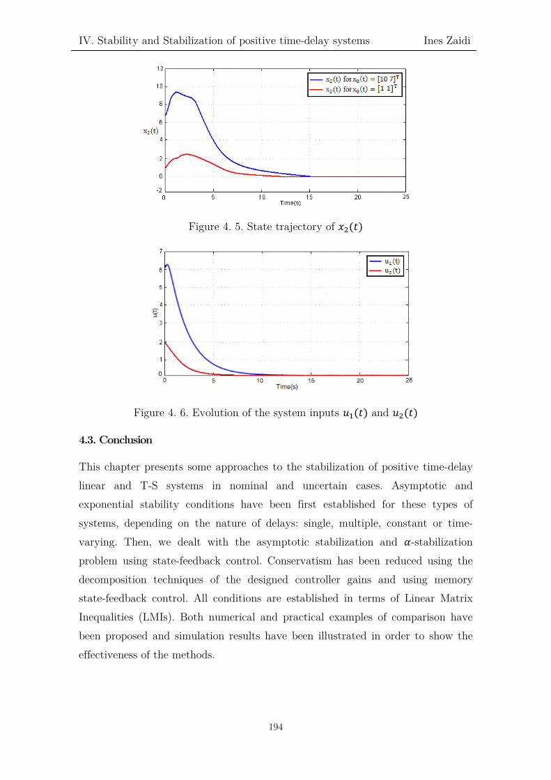
IV. Stability and Stabilization of positive time-delay systems Ines Zaidi
Figure 4. 5. State trajectory of 𝑥𝑥2(𝑡𝑡)
Figure 4. 6. Evolution of the system inputs 𝑢𝑢1(𝑡𝑡) and 𝑢𝑢2(𝑡𝑡)
4.3. Conclusion
This chapter presents some approaches to the stabilization of positive time-delay linear and T-S systems in nominal and uncertain cases. Asymptotic and exponential stability conditions have been first established for these types of systems, depending on the nature of delays: single, multiple, constant or time-varying. Then, we dealt with the asymptotic stabilization and 𝛼𝛼-stabilization problem using state-feedback control. Conservatism has been reduced using the decomposition techniques of the designed controller gains and using memory state-feedback control. All conditions are established in terms of Linear Matrix Inequalities (LMIs). Both numerical and practical examples of comparison have been proposed and simulation results have been illustrated in order to show the effectiveness of the methods.
194

V. Observers and Controllers for positive systems with time-delay Ines Zaidi
Chapter V
Observers and Controllers for Positive systems with time-delay
195

V. Observers and Controllers for positive systems with time-delay Ines Zaidi
196

V. Observers and Controllers for positive systems with time-delay Ines Zaidi
5.1. Introduction
In this chapter, we make a proposal for designing observer-based controllers for positive interval linear and T-S systems with time-delay. In this context, LMIs conditions are established by considering interval uncertainties. A positive interval observer is interesting since it can provide lower and upper estimates on the unmeasurable positive states. Also, it can guarantee the stability and positivity of the estimation error of the system. Firstly, we treat the problem of the design of positive observers for positive linear time-delay systems, with and without interval uncertainties. Secondly, we consider the positive observer-based controller design for positive interval linear systems with time-delay. Finally, we extend the previous works for positive interval T-S systems with time-delay, taking into account the nature of the premise variables of the system (measurable or unmeasurable). Numerical and practical examples have been illustrated to prove the effectiveness of the different proposed approaches.
5.2. Positive Observer design for Positive Linear systems with time-delay
5.2.1. POSITIVE OBSERVER DESIGN FOR POSITIVE AUTONOMOUS LINEAR
SYSTEMS WITH TIME-DELAY
In this section, we investigate the design of positive observers for positive time-delay linear systems. Conditions on the existence of positive observers are established, with the desired observer matrices constructed through the solution of LMIs. This problem has been treated by proposing a solution using LP techniques that reveal less efficient than LMI formulation (Li & Lam, 2012), (Rami et al, 2013).
Thus, we consider now the observer design of the following linear positive system with time-delay:
��̇�𝑥(𝑡𝑡) = 𝐴𝐴 𝑥𝑥(𝑡𝑡) + 𝐴𝐴1𝑥𝑥�𝑡𝑡 − 𝜏𝜏(𝑡𝑡)�𝑦𝑦(𝑡𝑡) = 𝐶𝐶 𝑥𝑥(𝑡𝑡) 𝑥𝑥(𝑡𝑡) = 𝜑𝜑(𝑡𝑡) ≽ 0, ∀ 𝑡𝑡 ∈ �−ℎ, 0�
(5.1)
where:
𝑥𝑥(𝑡𝑡) ∈ ℝ𝑛𝑛𝑥𝑥 is the state vector,
𝐴𝐴 ∈ ℝ𝑛𝑛𝑥𝑥×𝑛𝑛𝑥𝑥 is a Metzler matrix, 𝐴𝐴1 ∈ ℝ𝑛𝑛𝑥𝑥×𝑛𝑛𝑥𝑥 ≽ 0 and 𝐶𝐶 ∈ ℝ𝑛𝑛𝑦𝑦×𝑛𝑛𝑥𝑥 ≽ 0
197

V. Observers and Controllers for positive systems with time-delay Ines Zaidi
𝜏𝜏(𝑡𝑡) ∈ ℝ is the time-varying delay that is considered as a bounded continuous function as follows:
�0 ≤ 𝜏𝜏(𝑡𝑡) ≤ ℎ�̇�𝜏(𝑡𝑡) ≤ 𝑑𝑑 < 1
(5.2)
The Luenberger observer structure used in (Hof, 1998) is not suitable for such systems. For this reason, a more general observer structure will be adopted, of the following form:
𝑥𝑥�̇(𝑡𝑡) = 𝐺𝐺 𝑥𝑥�(𝑡𝑡) + 𝐺𝐺1𝑥𝑥��𝑡𝑡 − ℎ(𝑡𝑡)� + 𝐿𝐿 𝑦𝑦(𝑡𝑡) (5.3)
where 𝐺𝐺 ∈ ℝ𝑛𝑛𝑥𝑥×𝑛𝑛𝑥𝑥 , 𝐺𝐺1 ∈ ℝ𝑛𝑛𝑥𝑥×𝑛𝑛𝑥𝑥 and 𝐿𝐿 ∈ ℝ𝑛𝑛𝑥𝑥×𝑛𝑛𝑦𝑦 are the observer matrices to be determined. Throughout this section, we make the following assumption:
Assumption 5.1. The matrix 𝐴𝐴 is Hurwitz.
Define the error signal as 𝑒𝑒(𝑡𝑡) = 𝑥𝑥(𝑡𝑡) − 𝑥𝑥�(𝑡𝑡) (5.4)
We define the augmented state 𝑥𝑥� = [𝑒𝑒𝑇𝑇 𝑥𝑥𝑇𝑇]𝑇𝑇. Using (5.1) and (5.3), the dynamics of this augmented state are given by the following augmented system:
𝑥𝑥�̇(𝑡𝑡) = ��̇�𝑥(𝑡𝑡)�̇�𝑒(𝑡𝑡)� = 𝔸𝔸𝑚𝑚 𝑥𝑥�(𝑡𝑡) + 𝔸𝔸ℎ 𝑥𝑥�(𝑡𝑡 − ℎ(𝑡𝑡)) (5.5)
where 𝔸𝔸𝑚𝑚 = � 𝐴𝐴 0𝐴𝐴 − 𝐿𝐿𝐶𝐶 − 𝐺𝐺 𝐺𝐺� and 𝔸𝔸ℎ = � 𝐴𝐴1 0
𝐴𝐴1 − 𝐺𝐺1 𝐺𝐺1�
Based on this, we provide the conditions of design of a positive observer, in the following theorem:
Theorem 5.1. (Zaidi et al.)
For given scalars 𝛽𝛽 ≥ 0 and 𝑑𝑑 < 1 , the augmented system (5.5) is asymptotically stable and positive if there exist diagonal positive definite matrices 𝑃𝑃1, 𝑃𝑃2, 𝑄𝑄1 and 𝑄𝑄2, matrices 𝑌𝑌 ≽ 0, 𝑍𝑍1 ≽ 0 and 𝑍𝑍 Metzler such that the following conditions are satisfied:
⎝
⎜⎜⎜⎛
𝛺𝛺11 𝐼𝐼 𝛺𝛺12 0 𝐴𝐴1𝑇𝑇𝑃𝑃1 𝛺𝛺13
𝐼𝐼 −2𝐼𝐼 + 𝑄𝑄1 0 0 0 𝑍𝑍1𝑇𝑇
𝛺𝛺21 0 𝑍𝑍𝑇𝑇 + 𝑍𝑍 𝐼𝐼 0 00 0 𝐼𝐼 −2𝐼𝐼 + 𝑄𝑄2 0 0
𝑃𝑃1𝐴𝐴1 0 0 0 −(1 − 𝑑𝑑)𝑄𝑄1 0𝛺𝛺31 𝑍𝑍1 0 0 0 −(1 − 𝑑𝑑)𝑄𝑄2⎠
⎟⎟⎟⎞
< 0 (5.6)
198

V. Observers and Controllers for positive systems with time-delay Ines Zaidi
� 𝑃𝑃1𝐴𝐴 0𝑃𝑃2𝐴𝐴 − 𝑌𝑌𝐶𝐶 − 𝑍𝑍 𝑃𝑃2𝐺𝐺� + 𝛽𝛽𝐼𝐼 ≽ 0 (5.7)
� 𝑃𝑃1𝐴𝐴1 0𝑃𝑃2𝐴𝐴1 − 𝑍𝑍1 𝑍𝑍1
� ≽ 0 (5.8)
where:
𝛺𝛺11 = 𝐴𝐴𝑇𝑇𝑃𝑃1 + 𝑃𝑃1𝐴𝐴
𝛺𝛺12 = 𝛺𝛺21𝑇𝑇 = 𝐴𝐴𝑇𝑇𝑃𝑃2 − 𝐶𝐶𝑇𝑇𝑌𝑌𝑇𝑇 − 𝑍𝑍𝑇𝑇
𝛺𝛺13 = 𝛺𝛺13𝑇𝑇 = 𝐴𝐴1
𝑇𝑇𝑃𝑃2 − 𝑍𝑍1𝑇𝑇
Under these conditions, the desired observer matrices are obtained as follows:
𝐺𝐺 = 𝑃𝑃2−1𝑍𝑍 (5.9)
𝐺𝐺1 = 𝑃𝑃2−1 𝑍𝑍1 (5.10)
𝐿𝐿 = 𝑃𝑃2−1𝑌𝑌 (5.11)
Proof:
In order to make the augmented model (5.5) asymptotically stable, let us consider the Lyapunov–Krasovskii function:
𝑉𝑉(𝑥𝑥�(𝑡𝑡)) = 𝑉𝑉0�𝑥𝑥�(𝑡𝑡)� + 𝑉𝑉1�𝑥𝑥�(𝑡𝑡)� (5.12)
where
𝑉𝑉0(𝑥𝑥�(𝑡𝑡)) = 𝑥𝑥�(𝑡𝑡)𝑇𝑇𝑃𝑃𝑥𝑥�(𝑡𝑡) , 𝑃𝑃 = 𝑑𝑑𝑖𝑖𝑑𝑑𝑑𝑑[𝑃𝑃1 𝑃𝑃2] > 0 (5.13)
𝑉𝑉1�𝑥𝑥�(𝑡𝑡)� = � 𝑥𝑥�(𝑡𝑡)𝑇𝑇𝑄𝑄 𝑥𝑥�(𝑡𝑡) 𝑑𝑑𝑠𝑠𝑡𝑡
𝑡𝑡−ℎ(𝑡𝑡), 𝑄𝑄 = 𝑑𝑑𝑖𝑖𝑑𝑑𝑑𝑑[𝑄𝑄1 𝑄𝑄2] > 0 (5.14)
Its derivative with respect to time is given by:
�̇�𝑉(𝑥𝑥�(𝑡𝑡)) = 𝑥𝑥�̇(𝑡𝑡)𝑇𝑇𝑃𝑃𝑥𝑥�(𝑡𝑡) + 𝑥𝑥�(𝑡𝑡)𝑇𝑇𝑃𝑃𝑥𝑥�̇(𝑡𝑡) + 𝑥𝑥�(𝑡𝑡)𝑇𝑇𝑄𝑄 𝑥𝑥�(𝑡𝑡)
− �1 − ℎ̇(𝑡𝑡)� 𝑥𝑥��𝑡𝑡 − 𝜏𝜏(𝑡𝑡)�𝑇𝑇
𝑄𝑄 𝑥𝑥�(𝑡𝑡) (5.15)
Firstly, our goal is to guarantee the stability of the augmented system. The augmented time-delay system (5.5) is asymptotically stable if and only if:
�̇�𝑉(𝑥𝑥�(𝑡𝑡)) < 0 (5.16)
Then, we obtain the following inequality:
𝑥𝑥�(𝑡𝑡)𝑇𝑇�𝔸𝔸𝑚𝑚𝑇𝑇𝑃𝑃 + 𝑃𝑃 𝔸𝔸𝑚𝑚 + 𝑄𝑄�𝑥𝑥�(𝑡𝑡) + 𝑥𝑥��𝑡𝑡 − 𝜏𝜏(𝑡𝑡)�
𝑇𝑇 𝔸𝔸ℎ
𝑇𝑇𝑃𝑃 𝑥𝑥�(𝑡𝑡)
+𝑥𝑥�(𝑡𝑡)𝑇𝑇 𝑃𝑃 𝔸𝔸ℎ 𝑥𝑥��𝑡𝑡 − 𝜏𝜏(𝑡𝑡)� − �1 − �̇�𝜏(𝑡𝑡)�𝑥𝑥��𝑡𝑡 − 𝜏𝜏(𝑡𝑡)�𝑇𝑇
𝑄𝑄 𝑥𝑥��𝑡𝑡 − 𝜏𝜏(𝑡𝑡)� < 0 (5.17)
199

V. Observers and Controllers for positive systems with time-delay Ines Zaidi
Since, −�1 − �̇�𝜏(𝑡𝑡)� ≤ −(1 − 𝑑𝑑) < 0 (5.18)
Then, using Schur Complement (Annex B.2), the expression (5.17) becomes formulated in the following LMI:
�𝔸𝔸𝑚𝑚𝑇𝑇𝑃𝑃 + 𝑃𝑃 𝔸𝔸𝑚𝑚 + 𝑄𝑄 𝔸𝔸ℎ
𝑇𝑇𝑃𝑃𝑃𝑃𝔸𝔸ℎ −(1 − 𝑑𝑑)𝑄𝑄
� < 0 (5.19)
In order to facilitate the calculation of the observer gains 𝐿𝐿, 𝐺𝐺 and 𝐺𝐺1, the matrix variables 𝑃𝑃 > 0 and 𝑄𝑄 > 0 are chosen to be diagonal with respect to appropriate matrix blocks :
𝑃𝑃 = �𝑃𝑃1 00 𝑃𝑃2
� and 𝑄𝑄 = �𝑄𝑄1 00 𝑄𝑄2
� (5.20)
By substituting (5.20) into (5.19) and using the expressions of 𝔸𝔸𝑚𝑚 and 𝔸𝔸ℎ given in (5.5), we obtain:
⎝
⎜⎛
𝑆𝑆11 𝑆𝑆12 𝐴𝐴1𝑇𝑇𝑃𝑃1 𝑆𝑆13
𝑆𝑆12𝑇𝑇 𝑆𝑆22 0 𝐺𝐺1
𝑇𝑇𝑃𝑃2𝑃𝑃1𝐴𝐴1 0 −(1 − 𝑑𝑑)𝑄𝑄1 0𝑆𝑆13
𝑇𝑇 𝑃𝑃2𝐺𝐺1 0 −(1 − 𝑑𝑑)𝑄𝑄2⎠
⎟⎞
< 0 (5.21)
where:
𝑆𝑆11 = 𝐴𝐴𝑇𝑇𝑃𝑃1 + 𝑃𝑃1𝐴𝐴 + 𝑄𝑄1
𝑆𝑆12 = 𝐴𝐴𝑇𝑇𝑃𝑃2 − 𝐶𝐶𝑇𝑇𝐿𝐿𝑇𝑇𝑃𝑃2 − 𝐺𝐺𝑇𝑇𝑃𝑃2
𝑆𝑆22 = 𝐺𝐺𝑇𝑇𝑃𝑃2 + 𝑃𝑃2𝐺𝐺 + 𝑄𝑄2
𝑆𝑆13 = 𝐴𝐴1𝑇𝑇𝑃𝑃2 − 𝐺𝐺1
𝑇𝑇𝑃𝑃2
We replace 𝑌𝑌 = 𝑃𝑃2𝐿𝐿 , 𝑍𝑍 = 𝑃𝑃2𝐺𝐺 and 𝑍𝑍1 = 𝑃𝑃2𝐺𝐺1 from (5.9)-(5.11).
By applying the Schur complement, 𝑆𝑆11 is equivalent to the following LMI:
�𝐴𝐴𝑇𝑇𝑃𝑃1 + 𝑃𝑃1𝐴𝐴 𝐼𝐼
𝐼𝐼 −𝑄𝑄1−1� < 0 (5.22)
By applying the Schur complement to 𝑆𝑆22 , we get the following LMI:
�𝑍𝑍 + 𝑍𝑍𝑇𝑇 𝐼𝐼𝐼𝐼 −𝑄𝑄2
−1� < 0 (5.23)
The parameters 𝑃𝑃1, 𝑃𝑃2, 𝑄𝑄1, 𝑄𝑄2, 𝐺𝐺 = 𝑃𝑃2−1𝑍𝑍, 𝐺𝐺1 = 𝑃𝑃2
−1𝑍𝑍1 and 𝐿𝐿 = 𝑃𝑃2−1𝑌𝑌 are
obtained by solving LMIs in (5.6).
Secondly, the positivity of the augmented system (5.5) has to be taken into account. Therefore, we have to prove that 𝔸𝔸𝑚𝑚 is Metzler and 𝔸𝔸ℎ ≽ 0.
200

V. Observers and Controllers for positive systems with time-delay Ines Zaidi
We get then the following inequality from Definition 1.9 and Remark 1.1:
� 𝑃𝑃 𝔸𝔸𝑚𝑚 + 𝛽𝛽 𝐼𝐼 ≽ 0 , 𝑃𝑃𝔸𝔸ℎ ≽ 0 (5.24)
This implies that for the augmented system to be positive:
⎩⎪⎨
⎪⎧
𝑃𝑃1𝐴𝐴 + 𝛽𝛽 𝐼𝐼𝑛𝑛 ≽ 0 𝑃𝑃2𝐴𝐴 − 𝑌𝑌𝐶𝐶 − 𝑍𝑍 ≽ 0 𝑍𝑍 + 𝛽𝛽 𝐼𝐼𝑛𝑛 ≽ 0 𝑃𝑃1𝐴𝐴1 ≽ 0 𝑃𝑃2𝐴𝐴1 − 𝑍𝑍1 ≽ 0 𝑍𝑍1 ≽ 0
(5.25)
Finally, we get the following set of constraints for the augmented system to be positive:
⎩⎪⎨
⎪⎧
𝑃𝑃1𝐴𝐴 + 𝛽𝛽 𝐼𝐼𝑛𝑛 ≽ 0 𝑃𝑃2𝐴𝐴 − 𝑌𝑌𝐶𝐶 − 𝑍𝑍 ≽ 0 𝑍𝑍 + 𝛽𝛽 𝐼𝐼𝑛𝑛 ≽ 0 𝐴𝐴1 ≽ 0 𝐺𝐺1 ≽ 0 𝑃𝑃2𝐴𝐴1 − 𝑍𝑍1 ≽ 0
(5.26)
This concludes that the augmented system given in (5.5) is asymptotically stable and positive, which completes the proof.∎
5.2.2. POSITIVE OBSERVER DESIGN FOR POSITIVE INTERVAL LINEAR
SYSTEMS WITH TIME-DELAY
In this section, we consider the observer design of the following uncertain interval positive system with time-delay:
��̇�𝑥(𝑡𝑡) = 𝐴𝐴 𝑥𝑥(𝑡𝑡) + 𝐴𝐴1𝑥𝑥�𝑡𝑡 − 𝜏𝜏(𝑡𝑡)�𝑦𝑦(𝑡𝑡) = 𝐶𝐶 𝑥𝑥(𝑡𝑡) 𝑥𝑥(𝑡𝑡) = 𝜑𝜑(𝑡𝑡) ≽ 0, ∀ 𝑡𝑡 ∈ �−ℎ, 0�
(5.27)
where:
𝑥𝑥(𝑡𝑡) ∈ ℝ𝑛𝑛𝑥𝑥 is the state vector;
𝐴𝐴 ∈ ℝ𝑛𝑛𝑥𝑥×𝑛𝑛𝑥𝑥 is a Metzler matrix, 𝐴𝐴1 ∈ ℝ𝑛𝑛𝑥𝑥×𝑛𝑛𝑥𝑥 ≽ 0 and 𝐶𝐶 ∈ ℝ𝑛𝑛𝑦𝑦×𝑛𝑛𝑥𝑥 ≽ 0;
𝐴𝐴 ∈ [𝐴𝐴 , 𝐴𝐴], 𝐴𝐴1 ∈ [𝐴𝐴1, 𝐴𝐴1], 𝐶𝐶 ∈ [𝐶𝐶 , 𝐶𝐶], with 𝐴𝐴 , 𝐴𝐴, 𝐴𝐴1, 𝐴𝐴1, 𝐶𝐶 and 𝐶𝐶 known constant
matrices;
𝜏𝜏(𝑡𝑡) ∈ ℝ is the time-varying delay, a continuous function given by (5.2).
201

V. Observers and Controllers for positive systems with time-delay Ines Zaidi
By considering the proposed interval positive system with time-delay given in (5.27) and the observer structure proposed in (5.3), necessary and sufficient stability and positivity conditions are presented in the following theorem:
Theorem 5.2. (Zaidi et al.)
For given scalars 𝛽𝛽 ≥ 0 and 𝑑𝑑 < 1 , a positive robust observer of the form (5.3) exists for the uncertain system (5.27) if and only if there exist diagonal matrices 𝑃𝑃1 > 0, 𝑃𝑃2 > 0, 𝑄𝑄1 > 0, 𝑄𝑄2 > 0, and matrices 𝑌𝑌 ≽ 0, 𝑍𝑍1 ≽ 0 and 𝑍𝑍 Metzler, such that the following conditions hold:
⎝
⎜⎜⎜⎛
�̅�𝐴𝑇𝑇𝑃𝑃1 + 𝑃𝑃1�̅�𝐴 𝐼𝐼 �̅�𝐴𝑇𝑇𝑃𝑃2 − 𝐶𝐶𝑇𝑇𝑌𝑌𝑇𝑇 − 𝑍𝑍𝑇𝑇 0 𝐴𝐴1𝑇𝑇𝑃𝑃1 𝐴𝐴1
𝑇𝑇𝑃𝑃2 − 𝑍𝑍1
𝐼𝐼 −𝑄𝑄1−1 0 0 0 𝑍𝑍1
𝑇𝑇
𝑃𝑃2𝐴𝐴 − 𝑌𝑌𝐶𝐶 − 𝑍𝑍 0 𝑍𝑍𝑇𝑇 + 𝑍𝑍 𝐼𝐼 0 00 0 𝐼𝐼 −𝑄𝑄2
−1 0 0𝑃𝑃1𝐴𝐴1 0 0 0 −(1 − 𝑑𝑑)𝑄𝑄1 0
𝑃𝑃2𝐴𝐴1 − 𝑍𝑍1 𝑍𝑍1 0 0 0 −(1 − 𝑑𝑑)𝑄𝑄2⎠
⎟⎟⎟⎞
< 0 (5.28)
�𝑃𝑃1𝐴𝐴 0
𝑃𝑃2𝐴𝐴 − 𝑌𝑌𝐶𝐶 − 𝑍𝑍 𝑃𝑃2𝐺𝐺� + 𝛽𝛽𝐼𝐼 ≽ 0 (5.29)
�𝑃𝑃1𝐴𝐴1 0
𝑃𝑃2𝐴𝐴1 − 𝑍𝑍1 𝑍𝑍1� ≽ 0 (5.30)
Under these conditions, the desired observer matrices may be obtained by:
𝐿𝐿 = 𝑃𝑃2−1𝑌𝑌 , 𝐺𝐺 = 𝑃𝑃2
−1𝑍𝑍 and 𝐺𝐺1 = 𝑃𝑃2−1 𝑍𝑍1 (5.31)
Proof:
Sufficiency:
From (5.29), we obtain that 𝑌𝑌 ≠ 0. 𝑃𝑃2−1 is diagonally strictly positive. Therefore,
the obtained 𝐺𝐺 is Metzler and 𝐿𝐿 ≽ 0. 𝑍𝑍1 ≠ 0, then 𝐺𝐺1 ≽ 0 .
It follows from (5.29), (5.30) and (5.31) that:
𝑃𝑃2�𝐴𝐴 − 𝐿𝐿𝐶𝐶 − 𝐺𝐺� ≽ 0 (5.32)
which implies that: 𝐴𝐴 − 𝐿𝐿𝐶𝐶 − 𝐺𝐺 ≽ 0 (5.33)
For any 𝐴𝐴 ∈ �𝐴𝐴, 𝐴𝐴� and 𝐶𝐶 ∈ �𝐶𝐶, 𝐶𝐶�, as 𝐿𝐿 ≥ 0, it is obvious that:
𝐴𝐴 ≼ 𝐴𝐴 ≼ 𝐴𝐴 and 𝐿𝐿𝐶𝐶 ≼ 𝐿𝐿𝐶𝐶 ≼ 𝐿𝐿𝐶𝐶 (5.34)
202

V. Observers and Controllers for positive systems with time-delay Ines Zaidi
Combining (5.33) and (5.34), we get for any 𝐴𝐴 ∈ �𝐴𝐴, 𝐴𝐴� and 𝐶𝐶 ∈ �𝐶𝐶, 𝐶𝐶� :
𝐴𝐴 − 𝐿𝐿𝐶𝐶 − 𝐺𝐺 ≽ 𝐴𝐴 − 𝐿𝐿𝐶𝐶 − 𝐺𝐺 ≽ 0 (5.35)
with 𝐴𝐴 and 𝐺𝐺 are Metzler matrices.Thus, we conclude then that the matrix 𝔸𝔸𝑚𝑚 defined in (5.5) is Metzler.
Moreover, we have 𝐴𝐴1 ≽ 0 and 𝐺𝐺1 ≽ 0 .Thus, it follows from (5.30) that
𝑃𝑃2 𝐴𝐴1 − 𝑍𝑍1 = 𝑃𝑃2(𝐴𝐴1 − 𝐺𝐺1) ≽ 𝑃𝑃2�𝐴𝐴1 − 𝐺𝐺1� = 𝑃𝑃2 𝐴𝐴1 − 𝑍𝑍1 (5.36)
which implies that 𝐴𝐴1 − 𝐺𝐺1 ≽ 0 (5.37)
Then, the matrix 𝔸𝔸ℎ is nonegative.
The facts that 𝔸𝔸𝑚𝑚 is Metzler and 𝔸𝔸ℎ is nonnegative show that the augmented system (5.5) is a positive system.
From (5.28), we obtain that:
�𝔸𝔸𝑚𝑚𝑇𝑇
𝑃𝑃 + 𝑃𝑃 𝔸𝔸𝑚𝑚 + 𝑄𝑄 𝔸𝔸ℎ𝑇𝑇
𝑃𝑃∗ −(1 − 𝑑𝑑)𝑄𝑄
� < 0 (5.38)
where:
𝔸𝔸𝑚𝑚 = � 𝐴𝐴 0𝐴𝐴 − 𝐿𝐿𝐶𝐶 − 𝐺𝐺 𝐺𝐺
� and 𝔸𝔸ℎ = � 𝐴𝐴1 0𝐴𝐴1 − 𝐺𝐺1 𝐺𝐺1
�
Then, we obtain the following inequality:
�𝑃𝑃1 00 𝑃𝑃2
� � 𝐴𝐴 0𝐴𝐴 − 𝐿𝐿𝐶𝐶 − 𝐺𝐺 𝐺𝐺
� + � 𝐴𝐴 0𝐴𝐴 − 𝐿𝐿𝐶𝐶 − 𝐺𝐺 𝐺𝐺
�𝑇𝑇
�𝑃𝑃1 00 𝑃𝑃2
� + �𝑄𝑄1 00 𝑄𝑄2
� < 0
(5.39)
We get then the fact that:
𝜇𝜇 �� 𝐴𝐴 0𝐴𝐴 − 𝐿𝐿𝐶𝐶 − 𝐺𝐺 𝐺𝐺
�� < 0 (5.40)
Using (5.35), we get obviously that for any 𝐴𝐴 ∈ �𝐴𝐴, 𝐴𝐴� and 𝐶𝐶 ∈ �𝐶𝐶, 𝐶𝐶�,
� 𝐴𝐴 0𝐴𝐴 − 𝐿𝐿𝐶𝐶 − 𝐺𝐺 𝐺𝐺� ≼ � 𝐴𝐴 0
𝐴𝐴 − 𝐿𝐿𝐶𝐶 − 𝐺𝐺 𝐺𝐺� (5.41)
Then, combining (35), (39), (40) and by Lemma 3.2, we deduce that, for any 𝐴𝐴 ∈ �𝐴𝐴, 𝐴𝐴� and 𝐶𝐶 ∈ �𝐶𝐶, 𝐶𝐶� ,
𝜇𝜇 �� 𝐴𝐴 0𝐴𝐴 − 𝐿𝐿𝐶𝐶 − 𝐺𝐺 𝐺𝐺�� < 0 (5.42)
203
V. Observers and Controllers for positive systems with time-delay Ines Zaidi
which means that the augmented system (5.5) is asymptotically stable within the bounds of variation of 𝐴𝐴 and 𝐶𝐶.
Necessity:
Suppose that there exist 𝐺𝐺, 𝐺𝐺1 and 𝐿𝐿 such that the observer given in (5.3) is positive, i.e, 𝐺𝐺 is Metzler, 𝐿𝐿 ≽ 0 and 𝐺𝐺1 ≽ 0 and the augmented system (5.5) is a positive asymptotically stable system for any 𝐴𝐴 ∈ [𝐴𝐴 , 𝐴𝐴], 𝐴𝐴1 ∈ [𝐴𝐴1, 𝐴𝐴1] and 𝐶𝐶 ∈ [𝐶𝐶 , 𝐶𝐶].
Then, there exist diagonal positive matrices 𝑃𝑃1 , 𝑃𝑃2 , 𝑄𝑄1 and 𝑄𝑄2 such that:
�𝔸𝔸𝑚𝑚𝑇𝑇
𝑃𝑃 + 𝑃𝑃 𝔸𝔸𝑚𝑚 + 𝑄𝑄 𝔸𝔸ℎ𝑇𝑇
𝑃𝑃∗ −(1 − 𝑑𝑑)𝑄𝑄
� < 0 (5.43)
Then, the following inequality is obviously given:
�𝑃𝑃1 00 𝑃𝑃2
� � 𝐴𝐴 0𝐴𝐴 − 𝐿𝐿𝐶𝐶 − 𝐺𝐺 𝐺𝐺
� + � 𝐴𝐴 0𝐴𝐴 − 𝐿𝐿𝐶𝐶 − 𝐺𝐺 𝐺𝐺
�𝑇𝑇
�𝑃𝑃1 00 𝑃𝑃2
� + �𝑄𝑄1 00 𝑄𝑄2
� < 0
(5.44)
and
�𝑃𝑃1 00 𝑃𝑃2
� � 𝐴𝐴1 0𝐴𝐴1 − 𝐺𝐺1 𝐺𝐺1
� < 0 (5.45)
We have:
𝑌𝑌 = 𝑃𝑃2𝐿𝐿 , 𝑍𝑍 = 𝑃𝑃2𝐺𝐺 and 𝑍𝑍1 = 𝑃𝑃2𝐺𝐺1 (5.46)
We easily note, from the diagonal strict positivity of 𝑃𝑃2 , that 𝑍𝑍 is Metzler, 𝑌𝑌 ≽ 0 and 𝑍𝑍1 ≽ 0. If we substitute (5.46) in (5.44) and (5.45), we get the inequality given in (5.28).
Since the augmented delayed system (5.5) is positive for any 𝐴𝐴 ∈ [𝐴𝐴 , 𝐴𝐴] and 𝐶𝐶 ∈ [𝐶𝐶 , 𝐶𝐶], we obtain that:
�𝐴𝐴 0
𝐴𝐴 − 𝐿𝐿𝐶𝐶 − 𝐺𝐺 𝐺𝐺� is Metzler, which implies that 𝐴𝐴 − 𝐿𝐿𝐶𝐶 − 𝐺𝐺 ≽ 0. From the
positivity of 𝑃𝑃2 and (4.46), we further obtain that: 𝑃𝑃2𝐴𝐴 − 𝑌𝑌𝐶𝐶 − 𝑍𝑍 ≽ 0.
With the same manner, we get from the inequality given in (4.45) that:
𝑃𝑃2 𝐴𝐴1 − 𝑍𝑍1 ≽ 0 .
which proves the necessity.
204

V. Observers and Controllers for positive systems with time-delay Ines Zaidi
This completes the proof.∎
5.2.3. ILLUSTRATIVE EXAMPLE
This numerical example consists of a two-compartmental model of a biological system (Petrás & Magin, 2011) that does involve delays, as shown in Figure 5.1.
Figure 5. 1. Two-compartment model with the definition of model parameters
This system corresponds to the following time-delay system in the following form (5.27) where:
𝐴𝐴 = �−𝑑𝑑11 − 𝑑𝑑21 𝑑𝑑12
𝑑𝑑21 −𝑑𝑑22 − 𝑑𝑑12�, 𝐴𝐴1 = �
𝑑𝑑𝑑𝑑11 𝑑𝑑𝑑𝑑12𝑑𝑑𝑑𝑑21 𝑑𝑑𝑑𝑑22
�, 𝐵𝐵 = �𝑏𝑏1 00 𝑏𝑏2
�, 𝐶𝐶 = �𝑐𝑐1 00 𝑐𝑐2
�
Assume that the estimated parameters for this model are:
𝑑𝑑11 = 1.8195 ± 0.0431, 𝑑𝑑21 = 1.6510 ± 0.0630
𝑑𝑑12 = 2.1565 ± 0.0237, 𝑑𝑑22 = 1.2050 ± 0.1010
𝑑𝑑𝑑𝑑11 = 0.0412 ± 0.0021, 𝑑𝑑𝑑𝑑12 = 0.2145 ± 0.0035
𝑑𝑑𝑑𝑑21 = 0.1214 ± 0.0035, 𝑑𝑑𝑑𝑑22 = 0.0852 ± 0.0036
𝑏𝑏1 = 0.1 , 𝑏𝑏2 = 0.2, 𝑐𝑐1 = 𝑐𝑐2 = 1 ± 0.05
Then, by using the MATLAB LMI Toolbox, it can be seen that the conditions in Theorem 5.2. are feasible, for 𝑑𝑑 = 0.5 and 𝛽𝛽 = 2, with the following solution:
𝐺𝐺 = �−4.1239 1.19520.6454 −5.1407�, 𝐺𝐺1 = �0.0352 0.1523
0.0935 0.0741�, 𝐿𝐿 = �0.1951 0.45520.2892 0.8733�
205

V. Observers and Controllers for positive systems with time-delay Ines Zaidi
Figure 5. 2. The evolution of the interval estimates of 𝑥𝑥1(𝑡𝑡)
Figure 5. 3. The evolution of the interval estimates of 𝑥𝑥2(𝑡𝑡)
If we denote 𝑥𝑥𝑘𝑘𝑜𝑜𝑤𝑤𝑙𝑙𝑟𝑟 (𝑡𝑡) the evolution of the lower bound on the state from the initial condition 𝑥𝑥0 and 𝑥𝑥𝑢𝑢𝑝𝑝𝑝𝑝𝑙𝑙𝑟𝑟(𝑡𝑡) the evolution of the upper bound on the state
from the initial condition 𝑥𝑥0, then, the evolution of the estimated state 𝑥𝑥�(𝑡𝑡) will always be between the lower and upper states 𝑥𝑥𝑘𝑘𝑜𝑜𝑤𝑤𝑙𝑙𝑟𝑟 (𝑡𝑡) and 𝑥𝑥𝑢𝑢𝑝𝑝𝑝𝑝𝑙𝑙𝑟𝑟(𝑡𝑡). Moreover,
these states always remain nonnegative. These properties can be seen in Figures 5.2 and 5.3, that represent the state evolutions from the initial conditions (𝑥𝑥0 = [0.81 0.45]𝑇𝑇 and 𝑥𝑥0 = [0.12 0.05]𝑇𝑇). These facts show the effectiveness of
the proposed approach.
206

V. Observers and Controllers for positive systems with time-delay Ines Zaidi
5.3. Positive Observer-Based Controller design for Positive Interval Linear systems with time-delay
5.3.1. THEORETICAL APPROACH
We consider the interval positive time-delay system:
��̇�𝑥(𝑡𝑡) = 𝐴𝐴 𝑥𝑥(𝑡𝑡) + 𝐴𝐴1𝑥𝑥�𝑡𝑡 − 𝜏𝜏(𝑡𝑡)� + 𝐵𝐵 𝑢𝑢(𝑡𝑡)𝑦𝑦(𝑡𝑡) = 𝐶𝐶 𝑥𝑥(𝑡𝑡) 𝑥𝑥(𝑡𝑡) = 𝜑𝜑(𝑡𝑡) ≽ 0, ∀ 𝑡𝑡 ∈ �−ℎ, 0�
(5.47)
where:
𝑥𝑥(𝑡𝑡) ∈ ℝ𝑛𝑛𝑥𝑥 is the state vector,
𝑢𝑢(𝑡𝑡) ∈ ℝ𝑛𝑛𝑢𝑢 is the control vector,
𝐴𝐴 ∈ [𝐴𝐴 , 𝐴𝐴], 𝐴𝐴1 ∈ �𝐴𝐴1, 𝐴𝐴1�, 𝐵𝐵 ∈ [𝐵𝐵 , 𝐵𝐵] and 𝐶𝐶 ∈ [𝐶𝐶 , 𝐶𝐶] are unknown constant
matrices with known bounds, that fulfill 𝐴𝐴 ∈ ℝ𝑛𝑛𝑥𝑥×𝑛𝑛𝑥𝑥 is Metzler, 𝐴𝐴1 ∈ ℝ𝑛𝑛𝑥𝑥×𝑛𝑛𝑥𝑥 ≽
0 , 𝐵𝐵 ≽ 0 ∈ ℝ𝑛𝑛𝑥𝑥×𝑛𝑛𝑢𝑢 and 𝐶𝐶 ≽ 0 ∈ ℝ𝑛𝑛𝑦𝑦×𝑛𝑛𝑥𝑥.
𝜏𝜏(𝑡𝑡) ∈ ℝ is the time-varying delay: a differentiable continuous function, satisfying the following the conditions given in (5.2).
The following lemma provides conditions that guarantee the asymptotic stability and the positivity of the interval system (5.47).
Lemma 5.1. (Zaidi et al.)
If there exists a diagonal matrix 𝑅𝑅 = 𝑅𝑅𝑇𝑇 > 0 and a matrix 𝑆𝑆 = 𝑆𝑆𝑇𝑇 > 0 satisfying the following LMI:
�𝑅𝑅𝐴𝐴 + 𝐴𝐴𝑇𝑇
𝑅𝑅 + 𝑆𝑆 𝑅𝑅𝐴𝐴1∗ −(1 − 𝑑𝑑)𝑆𝑆
� < 0 (5.48)
then, the interval system (5.47) is positive and asymptotically stable.
Proof:
We have 𝐴𝐴 ≼ 𝐴𝐴, 𝐴𝐴1 ≼ 𝐴𝐴1 and 𝑅𝑅 > 0 with 𝑅𝑅 diagonal; then, 𝑅𝑅𝐴𝐴 ≼ 𝑅𝑅𝐴𝐴 and
𝑅𝑅𝐴𝐴1 ≼ 𝑅𝑅𝐴𝐴1. Moreover, we have: 𝑅𝑅𝐴𝐴 + 𝐴𝐴𝑇𝑇𝑅𝑅 + 𝑆𝑆 ≼ 𝑅𝑅𝐴𝐴 + 𝐴𝐴𝑇𝑇
𝑅𝑅 + 𝑆𝑆 for any matrix 𝑆𝑆, which means that:
�𝑅𝑅𝐴𝐴 + 𝐴𝐴𝑇𝑇𝑅𝑅 + 𝑆𝑆 𝑅𝑅𝐴𝐴1∗ −(1 − 𝑑𝑑)𝑆𝑆� ≼ �𝑅𝑅𝐴𝐴 + 𝐴𝐴
𝑇𝑇𝑅𝑅 + 𝑆𝑆 𝑅𝑅𝐴𝐴1
∗ −(1 − 𝑑𝑑)𝑆𝑆� (5.49)
207

V. Observers and Controllers for positive systems with time-delay Ines Zaidi
From (5.48) and (5.49) and using (4.12), we deduce that the existence of a diagonal matrix 𝑅𝑅 = 𝑅𝑅𝑇𝑇 > 0 and a matrix 𝑆𝑆 = 𝑆𝑆𝑇𝑇 > 0 satisfying LMI (5.48) implies the feasibility of the following LMI with the same matrices 𝑅𝑅 and 𝑆𝑆:
�𝑅𝑅𝐴𝐴 + 𝐴𝐴𝑇𝑇𝑅𝑅 + 𝑆𝑆 𝑅𝑅𝐴𝐴1∗ −(1 − 𝑑𝑑)𝑆𝑆� < 0 (5.50)
Then, the system (5.47) is asymptotically stable.
Moreover, system (5.47) is defined by its matrices that fulfill 𝐴𝐴 ∈ [𝐴𝐴 , 𝐴𝐴],
𝐴𝐴1 ∈ �𝐴𝐴1, 𝐴𝐴1�, 𝐵𝐵 ∈ [𝐵𝐵 , 𝐵𝐵] and 𝐶𝐶 ∈ [𝐶𝐶 , 𝐶𝐶]. Since 𝐴𝐴 ∈ ℝ𝑛𝑛×𝑛𝑛 is Metzler, 𝐴𝐴1 ≽ 0 ,
𝐵𝐵 ≽ 0 and 𝐶𝐶 ≽ 0, we deduce that 𝐴𝐴 ∈ ℝ𝑛𝑛𝑥𝑥×𝑛𝑛𝑥𝑥 is Metzler, 𝐴𝐴1 ≽ 0 , 𝐵𝐵 ≽ 0
and 𝐶𝐶 ≽ 0, which means that system (5.47) is positive.
Both of the previous facts conclude that system (5.47) is positive and asymptotically stable. ∎
We use the following observer defined by:
𝑥𝑥�̇(𝑡𝑡) = 𝐺𝐺 𝑥𝑥�(𝑡𝑡) + 𝐺𝐺1𝑥𝑥��𝑡𝑡 − 𝜏𝜏(𝑡𝑡)� + 𝐿𝐿 𝑦𝑦(𝑡𝑡) (5.51)
where 𝐺𝐺 ∈ ℝ𝑛𝑛𝑥𝑥×𝑛𝑛𝑥𝑥, 𝐺𝐺1 ∈ ℝ𝑛𝑛𝑥𝑥×𝑛𝑛𝑥𝑥, 𝐿𝐿 ∈ ℝ𝑛𝑛𝑥𝑥×𝑛𝑛𝑦𝑦 are the observer matrices to be determined.
The static state-feedback control law used is given by the following expression:
𝑢𝑢(𝑡𝑡) = 𝐾𝐾𝑥𝑥�(𝑡𝑡) (5.52)
where 𝐾𝐾 ∈ ℝ𝑛𝑛𝑢𝑢×𝑛𝑛𝑥𝑥 is the controller matrix to be determined.
Then, the closed-loop system is written as follows:
⎩⎪⎨
⎪⎧�̇�𝑥(𝑡𝑡) = 𝐴𝐴 𝑥𝑥(𝑡𝑡) + 𝐴𝐴1𝑥𝑥�𝑡𝑡 − 𝜏𝜏(𝑡𝑡)� + 𝐵𝐵 𝐾𝐾𝑥𝑥�(𝑡𝑡)
𝑦𝑦(𝑡𝑡) = 𝐶𝐶 𝑥𝑥(𝑡𝑡) 𝑥𝑥(𝑡𝑡) = 𝜑𝜑(𝑡𝑡) ≽ 0, ∀ 𝑡𝑡 ∈ �−ℎ, 0� 𝑥𝑥�(𝑡𝑡) = 𝜗𝜗(𝑡𝑡) ≽ 0, ∀ 𝑡𝑡 ∈ �−ℎ, 0�
(5.53)
To ensure the positivity of the state estimation, the key lies in the nonnegativity of the error, which is defined by:
𝑒𝑒(𝑡𝑡) = 𝑥𝑥(𝑡𝑡) − 𝑥𝑥�(𝑡𝑡) (5.54)
If we choose [𝑥𝑥𝑇𝑇(𝑡𝑡) 𝑒𝑒𝑇𝑇(𝑡𝑡)]𝑇𝑇 as the new augmented state variable, then the augmented system will become:
208

V. Observers and Controllers for positive systems with time-delay Ines Zaidi
��̇�𝑥(𝑡𝑡)�̇�𝑒(𝑡𝑡)
� = 𝐴𝐴𝑚𝑚 �𝑥𝑥(𝑡𝑡)𝑒𝑒(𝑡𝑡)� + 𝐴𝐴ℎ �
𝑥𝑥(𝑡𝑡 − ℎ(𝑡𝑡)𝑒𝑒(𝑡𝑡 − ℎ(𝑡𝑡))� (5.55)
where:
𝐴𝐴𝑚𝑚 = � 𝐴𝐴 + 𝐵𝐵𝐾𝐾 −𝐵𝐵𝐾𝐾𝐴𝐴 − 𝐿𝐿𝐶𝐶 + 𝐵𝐵𝐾𝐾 − 𝐺𝐺 𝐺𝐺 − 𝐵𝐵𝐾𝐾� (5.56)
and
𝐴𝐴ℎ = � 𝐴𝐴1 0𝐴𝐴1 − 𝐺𝐺1 𝐺𝐺1
� (5.57)
The problem to be solved is to find 𝐺𝐺, 𝐺𝐺1, 𝐿𝐿 and 𝐾𝐾 such that the augmented system (5.55) is positive and asymptotically stable. Meanwhile, to guarantee the nonnegativity of the estimate 𝑥𝑥�(𝑡𝑡), it is obvious to require that 𝐺𝐺 is Metzler and 𝐿𝐿 is nonnegative. The following theorem provides a necessary condition for the existence of solutions to the problem of a continuous-time observer-based controller.
Theorem 5.3. (Zaidi et al.)
If there exists a static state-feedback controller (5.52) that stabilizes system (5.47), using the observer (5.51) with a positive augmented system (5.55), then the following inequalities with respect to Metzler 𝐺𝐺, 𝐺𝐺1 ≽ 0, 𝐿𝐿 ≽ 0 and 𝐾𝐾 ≼ 0 have a solution:
𝑡𝑡𝑟𝑟𝑑𝑑𝑐𝑐𝑒𝑒�𝐴𝐴 + 𝐺𝐺 + (𝐵𝐵 − 𝐵𝐵)𝐾𝐾� < 0 (5.58)
[𝐴𝐴 + 𝐵𝐵𝐾𝐾]𝑚𝑚𝑖𝑖 ≥ 0 , 1 ≤ 𝑖𝑖 ≠ 𝑗𝑗 ≤ 𝑛𝑛 (5.59)
[𝐺𝐺 − 𝐵𝐵𝐾𝐾]𝑚𝑚𝑖𝑖 ≥ 0 , 1 ≤ 𝑖𝑖 ≠ 𝑗𝑗 ≤ 𝑛𝑛 (5.60)
𝐴𝐴 − 𝐿𝐿𝐶𝐶 + 𝐵𝐵𝐾𝐾 − 𝐺𝐺 ≽ 0 (5.61)
𝐴𝐴1 − 𝐺𝐺1 ≽ 0 (5.62)
Proof:
If there exists such observer-based controller, then, from (5.55), we have that
𝜇𝜇 �� 𝐴𝐴 + 𝐵𝐵𝐾𝐾 −𝐵𝐵𝐾𝐾𝐴𝐴 − 𝐿𝐿𝐶𝐶 + 𝐵𝐵𝐾𝐾 − 𝐺𝐺 𝐺𝐺 − 𝐵𝐵𝐾𝐾�� < 0 (5.63)
and � 𝐴𝐴 + 𝐵𝐵𝐾𝐾 −𝐵𝐵𝐾𝐾𝐴𝐴 − 𝐿𝐿𝐶𝐶 + 𝐵𝐵𝐾𝐾 − 𝐺𝐺 𝐺𝐺 − 𝐵𝐵𝐾𝐾� is Metzler (5.64)
As we have that:
209

V. Observers and Controllers for positive systems with time-delay Ines Zaidi
�𝐴𝐴 + 𝐵𝐵𝐾𝐾 −𝐵𝐵𝐾𝐾
𝐴𝐴 − 𝐿𝐿𝐶𝐶 + 𝐵𝐵𝐾𝐾 − 𝐺𝐺 𝐺𝐺 − 𝐵𝐵𝐾𝐾� ≼ � 𝐴𝐴 + 𝐵𝐵𝐾𝐾 −𝐵𝐵𝐾𝐾
𝐴𝐴 − 𝐿𝐿𝐶𝐶 + 𝐵𝐵𝐾𝐾 − 𝐺𝐺 𝐺𝐺 − 𝐵𝐵𝐾𝐾�
≼ �𝐴𝐴 + 𝐵𝐵𝐾𝐾 −𝐵𝐵𝐾𝐾
𝐴𝐴 − 𝐿𝐿𝐶𝐶 + 𝐵𝐵𝐾𝐾 − 𝐺𝐺 𝐺𝐺 − 𝐵𝐵𝐾𝐾� (5.65)
Then, we deduce that
𝜇𝜇 ��𝐴𝐴 + 𝐵𝐵𝐾𝐾 −𝐵𝐵𝐾𝐾
𝐴𝐴 − 𝐿𝐿𝐶𝐶 + 𝐵𝐵𝐾𝐾 − 𝐺𝐺 𝐺𝐺 − 𝐵𝐵𝐾𝐾�� < 0 (5.66)
and
�𝐴𝐴 + 𝐵𝐵𝐾𝐾 −𝐵𝐵𝐾𝐾
𝐴𝐴 − 𝐿𝐿𝐶𝐶 + 𝐵𝐵𝐾𝐾 − 𝐺𝐺 𝐺𝐺 − 𝐵𝐵𝐾𝐾� is Metzler (5.67)
It follows from (5.66) that
𝑡𝑡𝑟𝑟𝑑𝑑𝑐𝑐𝑒𝑒 ��𝐴𝐴 + 𝐵𝐵𝐾𝐾 −𝐵𝐵𝐾𝐾
𝐴𝐴 − 𝐿𝐿𝐶𝐶 + 𝐵𝐵𝐾𝐾 − 𝐺𝐺 𝐺𝐺 − 𝐵𝐵𝐾𝐾�� < 0 (5.68)
which is equivalent to (5.58). Moreover, it is obvious that (5.67) is equivalent to (5.59), (5.60) and (5.61). Moreover, the fact that 𝐴𝐴ℎℎ ≽ 0 implies (5.62), which completes the proof.∎
Thus, we now study sufficient conditions and the corresponding synthesis approach for this problem in this theorem which guarantees the asymptotic stability and the positivity of the augmented system (5.47).
Theorem 5.4. (Zaidi et al.)
There exists an observer-based controller (5.51)-(5.52) for the system (5.47) that provides asymptotic stability and positivity of the augmented system (5.55) if there exists a positive scalar 𝜀𝜀 and matrices 𝑃𝑃 = 𝑑𝑑𝑖𝑖𝑑𝑑𝑑𝑑[𝑃𝑃1 𝑃𝑃2] > 0, 𝑄𝑄 =
𝑑𝑑𝑖𝑖𝑑𝑑𝑑𝑑[𝑄𝑄1 𝑄𝑄2] > 0, a Metzler matrix 𝐺𝐺, 𝐺𝐺1 ≽ 0, 𝐿𝐿 ≽ 0 and 𝐾𝐾 ≼ 0 such that:
�
𝔸𝔸 𝐴𝐴ℎ𝑇𝑇𝑃𝑃 𝑃𝑃ℬ + 𝒞𝒞𝑇𝑇𝒦𝒦𝑇𝑇 𝜀𝜀ℬ
∗ −(1 − 𝑑𝑑)𝑄𝑄 0 0∗ 0 −𝐼𝐼 0∗ ∗ ∗ −𝐼𝐼
� < 0 (5.70)
[𝐴𝐴 + 𝐵𝐵𝐾𝐾]𝑚𝑚𝑖𝑖 ≥ 0 , 1 ≤ 𝑖𝑖 ≠ 𝑗𝑗 ≤ 𝑛𝑛 (5.71)
[𝐺𝐺 − 𝐵𝐵𝐾𝐾]𝑚𝑚𝑖𝑖 ≥ 0 , 1 ≤ 𝑖𝑖 ≠ 𝑗𝑗 ≤ 𝑛𝑛 (5.72)
𝐴𝐴 − 𝐿𝐿𝐶𝐶 + 𝐵𝐵𝐾𝐾 − 𝐺𝐺 ≽ 0, (5.73)
210

V. Observers and Controllers for positive systems with time-delay Ines Zaidi
𝐴𝐴1 − 𝐺𝐺1 ≽ 0 (5.74)
where:
𝔸𝔸 = 𝒜𝒜𝑇𝑇𝑃𝑃 + 𝑃𝑃𝒜𝒜 − 𝜀𝜀ℬℬ𝑇𝑇𝑃𝑃 − 𝜀𝜀𝑃𝑃ℬ𝑇𝑇ℬ + 𝑄𝑄
𝒜𝒜 = �𝐴𝐴 0𝐴𝐴 0
� , ℬ = �0 𝐵𝐵 − 𝐵𝐵 0 𝐵𝐵0 𝐵𝐵 − 𝐵𝐵 −𝐼𝐼 𝐵𝐵
�
𝒦𝒦 = �
𝐺𝐺 𝐿𝐿 0 0𝐾𝐾 0 0 00 0 𝐺𝐺 𝐿𝐿0 0 𝐾𝐾 0
� 𝒞𝒞 = �
0 𝐼𝐼0 0𝐼𝐼 −𝐼𝐼𝐶𝐶 0
� (5.75)
Proof:
It follows from (5.71) that 𝐴𝐴 + 𝐵𝐵𝐾𝐾 is Metzler. Combining this with 𝐾𝐾 ≼ 0 and
𝐿𝐿 ≽ 0 yields, for any 𝐴𝐴 ∈ [𝐴𝐴, 𝐴𝐴], 𝐵𝐵 ∈ [𝐵𝐵, 𝐵𝐵] and 𝐶𝐶 ∈ [𝐶𝐶, 𝐶𝐶], that:
𝐴𝐴 + 𝐵𝐵𝐾𝐾 ≽ 𝐴𝐴 + 𝐵𝐵𝐾𝐾 is Metzler (5.76)
𝐴𝐴 − 𝐿𝐿𝐶𝐶 + 𝐵𝐵𝐾𝐾 − 𝐺𝐺 ≽ 𝐴𝐴 − 𝐿𝐿𝐶𝐶 + 𝐵𝐵𝐾𝐾 − 𝐺𝐺 ≽ 0 (5.77)
In addition, from 𝐺𝐺 being Metzler and 𝐾𝐾 ≼ 0 , we obtain that, for any 𝐵𝐵 ∈ [𝐵𝐵, 𝐵𝐵]: −𝐵𝐵𝐾𝐾 ≽ 0 (5.78)
𝐺𝐺 − 𝐵𝐵𝐾𝐾 is Metzler (5.79)
Therefore, from (5.76)-(5.79) and the fact that 𝐴𝐴ℎ ≽ 0, we have that, for any 𝐴𝐴 ∈ [𝐴𝐴, 𝐴𝐴], 𝐵𝐵 ∈ [𝐵𝐵, 𝐵𝐵] and 𝐶𝐶 ∈ [𝐶𝐶, 𝐶𝐶], the augmented system (5.55) is positive.
It follows from (5.70), by the Schur complement, that:
� ℵ1 𝐴𝐴ℎ𝑇𝑇𝑃𝑃
𝑃𝑃𝐴𝐴ℎ −(1 − 𝑑𝑑)𝑄𝑄� < 0 (5.80)
where:
ℵ1 = 𝒜𝒜𝑇𝑇𝑃𝑃 + 𝑃𝑃𝒜𝒜 − 𝜀𝜀ℬℬ𝑇𝑇𝑃𝑃 − 𝜀𝜀𝑃𝑃ℬ𝑇𝑇ℬ + 𝜀𝜀2ℬℬ𝑇𝑇 + (ℬ𝑇𝑇𝑃𝑃 + 𝒦𝒦 𝒞𝒞)𝑇𝑇(ℬ𝑇𝑇𝑃𝑃 + 𝒦𝒦 𝒞𝒞) + 𝑄𝑄
We have then:
𝒜𝒜𝑇𝑇𝑃𝑃 + 𝑃𝑃𝒜𝒜 − 𝜀𝜀ℬℬ𝑇𝑇𝑃𝑃 − 𝜀𝜀𝑃𝑃ℬ𝑇𝑇ℬ + 𝜀𝜀2ℬℬ𝑇𝑇 + (ℬ𝑇𝑇𝑃𝑃 + 𝒦𝒦 𝒞𝒞)𝑇𝑇(ℬ𝑇𝑇𝑃𝑃 + 𝒦𝒦 𝒞𝒞) + 𝑄𝑄 < 0
(5.81)
Taking into account the following relationship:
𝑃𝑃𝐵𝐵𝐵𝐵𝑇𝑇𝑃𝑃 − 𝜀𝜀𝐵𝐵𝐵𝐵𝑇𝑇𝑃𝑃 − 𝜀𝜀𝑃𝑃𝐵𝐵𝑇𝑇𝐵𝐵 + 𝜀𝜀2𝐵𝐵𝐵𝐵𝑇𝑇 = (𝑃𝑃𝐵𝐵 −𝜀𝜀 𝐵𝐵)(𝐵𝐵𝑇𝑇𝑃𝑃 − 𝜀𝜀𝐵𝐵𝑇𝑇) ≥ 0 (5.82)
we obtain, from (5.81) the following inequality:
211

V. Observers and Controllers for positive systems with time-delay Ines Zaidi
𝒜𝒜𝑇𝑇𝑃𝑃 + 𝑃𝑃𝒜𝒜 − 𝑃𝑃ℬℬ𝑇𝑇𝑃𝑃 + (ℬ𝑇𝑇𝑃𝑃 + 𝒦𝒦 𝒞𝒞)𝑇𝑇(ℬ𝑇𝑇𝑃𝑃 + 𝒦𝒦 𝒞𝒞) + 𝑄𝑄 < 0 (5.83)
Rewriting (5.83) yields that:
(𝒜𝒜 + ℬ𝒦𝒦𝒞𝒞)𝑇𝑇𝑃𝑃 + 𝑃𝑃(𝒜𝒜 + ℬ𝒦𝒦𝒞𝒞) + 𝒞𝒞𝑇𝑇𝒦𝒦𝑇𝑇𝒦𝒦 𝒞𝒞 + 𝑄𝑄 < 0 (5.84)
which implies that:
(𝒜𝒜 + ℬ𝒦𝒦𝒞𝒞)𝑇𝑇𝑃𝑃 + 𝑃𝑃(𝒜𝒜 + ℬ𝒦𝒦𝒞𝒞) + 𝑄𝑄 < 0 (5.85)
Therefore, we get: 𝜇𝜇(𝒜𝒜 + ℬ𝒦𝒦𝒞𝒞) < 0 (5.86)
Replacing ℵ1 with (5.85) in (5.80), we get:
�(𝒜𝒜 + ℬ𝒦𝒦𝒞𝒞)𝑇𝑇𝑃𝑃 + 𝑃𝑃(𝒜𝒜 + ℬ𝒦𝒦𝒞𝒞) + 𝑄𝑄 𝐴𝐴ℎℎ𝑇𝑇 𝑃𝑃
𝑃𝑃𝐴𝐴ℎℎ −(1 − 𝑑𝑑)𝑄𝑄� < 0 (5.87)
Some algebraic manipulations, using (5.75), lead to:
𝒜𝒜 + ℬ𝒦𝒦𝒞𝒞 = �𝐴𝐴 + 𝐵𝐵𝐾𝐾 −𝐵𝐵𝐾𝐾
𝐴𝐴 − 𝐿𝐿𝐶𝐶 + 𝐵𝐵𝐾𝐾 − 𝐺𝐺 𝐺𝐺 − 𝐵𝐵𝐾𝐾� (5.88)
In addition, it is easy to show that:
�𝐴𝐴 + 𝐵𝐵𝐾𝐾 −𝐵𝐵𝐾𝐾
𝐴𝐴 − 𝐿𝐿𝐶𝐶 + 𝐵𝐵𝐾𝐾 − 𝐺𝐺 𝐺𝐺 − 𝐵𝐵𝐾𝐾� ≽ � 𝐴𝐴 + 𝐵𝐵𝐾𝐾 −𝐵𝐵𝐾𝐾
𝐴𝐴 − 𝐿𝐿𝐶𝐶 + 𝐵𝐵𝐾𝐾 − 𝐺𝐺 𝐺𝐺 − 𝐵𝐵𝐾𝐾� (5.89)
Therefore, by combining (5.86)-(5.89), we obtain that:
𝜇𝜇 �� 𝐴𝐴 + 𝐵𝐵𝐾𝐾 −𝐵𝐵𝐾𝐾𝐴𝐴 − 𝐿𝐿𝐶𝐶 + 𝐵𝐵𝐾𝐾 − 𝐺𝐺 𝐺𝐺 − 𝐵𝐵𝐾𝐾�� < 0 (5.90)
which means that (5.55) is asymptotically stable for any 𝐴𝐴 ∈ [𝐴𝐴, 𝐴𝐴], 𝐵𝐵 ∈ [𝐵𝐵, 𝐵𝐵]
and 𝐶𝐶 ∈ [𝐶𝐶, 𝐶𝐶].
This completes the proof.∎
5.3.2. ILLUSTRATIVE EXAMPLE
This numerical example is based on a compartmental system that involves delays, as shown in Figure 5.1 where the system parameters are:
𝐴𝐴 = �−(𝑑𝑑11 + 𝑑𝑑21) 𝑑𝑑12
𝑑𝑑21 −(𝑑𝑑22 + 𝑑𝑑12)�, 𝐴𝐴1 = �𝑑𝑑𝑑𝑑11 𝑑𝑑𝑑𝑑12𝑑𝑑𝑑𝑑21 𝑑𝑑𝑑𝑑22
�
𝐵𝐵 = �1 00 1�, 𝐶𝐶 = [𝑐𝑐11 0]
The elements of the bounded matrices 𝐴𝐴, 𝐴𝐴, 𝐶𝐶 and 𝐶𝐶 are obtained from:
𝑑𝑑11 = 1.2 ± 0.042, 𝑑𝑑12 = 0.3 ± 0.061, 𝑑𝑑21 = 0.5 ± 0.045, 𝑑𝑑22 = 0.6 ± 0.140,
212
V. Observers and Controllers for positive systems with time-delay Ines Zaidi
𝑑𝑑𝑑𝑑11 = 0.05 ± 0.005, 𝑑𝑑𝑑𝑑12 = 0.01 ± 0.005,
𝑑𝑑𝑑𝑑21 = 0.08 ± 0.005, 𝑑𝑑𝑑𝑑22 = 0.06 ± 0.005, 𝑐𝑐11 = 1 ± 0.1.
𝜏𝜏1(𝑡𝑡) = 0.25 + 0.14 𝑠𝑠𝑖𝑖𝑛𝑛 (𝑡𝑡), bounded by ℎ = 0.39.
Then, it can be seen that the conditions in Theorems 5.3 and 5.4 are feasible, for 𝜀𝜀 = 15, ℎ = 0.39 and 𝑑𝑑 = 0.5, with the following solution, obtained by using the Scilab 5.3.3 LMI toolbox:
𝑃𝑃1 = � 240.8184 −214.7411−214.7411 222.8628 �,
𝑃𝑃2 = � 151.2631 −201.4101−165.0750 101.6504 �
𝑄𝑄1 = � 347.6394 −256.5724−256.5724 205.6603 �,
𝑄𝑄2 = � 82.9465 −21.2129−21.2129 79.4133 �
𝐺𝐺 = �−12.3163 5.84046.3600 −11.5066�, 𝐺𝐺1 = �0.0250 0.0049
0.0400 0.0300�
𝐿𝐿 = � 6.585215.8514�, 𝐾𝐾 = �−0.2824 −0.1117
−1.6278 −0.6251�
The simulations presented in Figures 5.4 to 5.6 show that the real state vector 𝑥𝑥(𝑡𝑡), as well as the estimated state vector 𝑥𝑥�(𝑡𝑡), are nonnegative and converge. These properties can be seen in Figures 5.4 and 5.5, which represent the state evolutions from given initial conditions 𝑥𝑥0 = [6.7 8]𝑇𝑇 and 𝑥𝑥�0 = [5 4]𝑇𝑇, for
𝑡𝑡 ∈ [−0.39 0], when 𝐴𝐴 = 𝐴𝐴, 𝐵𝐵 = 𝐵𝐵, 𝐶𝐶 = 𝐶𝐶, 𝐴𝐴1 = 𝐴𝐴1 and ℎ = 0.39. It is possible to see, from Figure 5.6, that the estimation errors are nonnegative. These facts show the effectiveness of the proposed approach.
213
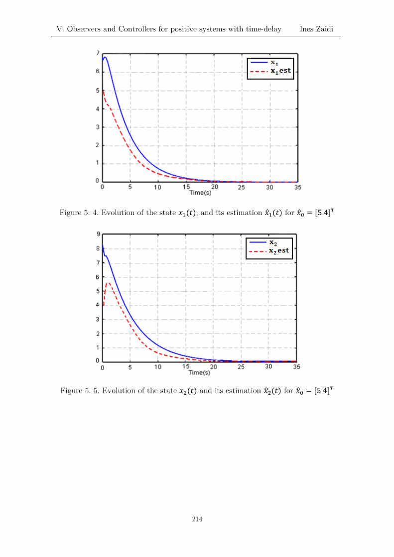
V. Observers and Controllers for positive systems with time-delay Ines Zaidi
Figure 5. 4. Evolution of the state 𝑥𝑥1(𝑡𝑡), and its estimation 𝑥𝑥�1(𝑡𝑡) for 𝑥𝑥�0 = [5 4]𝑇𝑇
Figure 5. 5. Evolution of the state 𝑥𝑥2(𝑡𝑡) and its estimation 𝑥𝑥�2(𝑡𝑡) for 𝑥𝑥�0 = [5 4]𝑇𝑇
214

V. Observers and Controllers for positive systems with time-delay Ines Zaidi
Figure 5. 6. Evolution of the estimation errors 𝑒𝑒1(𝑡𝑡) and 𝑒𝑒2(𝑡𝑡) for 𝑥𝑥0 = [6.7 8]𝑇𝑇 and 𝑥𝑥�0 = [5 4]𝑇𝑇
5.4. Positive Observer-Based Controller design for Positive Interval T-S systems with time-delay
In this section, we are interested in the synthesis of positive observer-based controllers for positive interval T-S systems with time-delay. We will study both cases: when the decision variables of the system are measurable and when they are unmeasurable.
5.4.1. CASE 1: MEASURABLE PREMISE VARIABLES
We consider the observer design for the following interval positive time-delay T-S system:
⎩⎪⎪⎨
⎪⎪⎧�̇�𝑥(𝑡𝑡) = � ℎ𝑚𝑚(𝑧𝑧(𝑡𝑡))(𝐴𝐴𝑚𝑚 𝑥𝑥(𝑡𝑡) + 𝐴𝐴1𝑚𝑚𝑥𝑥(𝑡𝑡 − 𝜏𝜏𝑚𝑚(𝑡𝑡)) + 𝐵𝐵𝑚𝑚 𝑢𝑢(𝑡𝑡))
𝑟𝑟
𝑚𝑚=1
𝑦𝑦(𝑡𝑡) = � ℎ𝑚𝑚(𝑧𝑧(𝑡𝑡))𝑟𝑟
𝑚𝑚=1
𝐶𝐶𝑚𝑚 𝑥𝑥(𝑡𝑡)
𝑥𝑥(𝑡𝑡) = 𝜑𝜑(𝑡𝑡) ≽ 0, ∀ 𝑡𝑡 ∈ �−ℎ, 0�
(5.91)
where:
𝑥𝑥(𝑡𝑡) ∈ ℝ𝑛𝑛𝑥𝑥 is the state vector,
𝑢𝑢(𝑡𝑡) ∈ ℝ𝑛𝑛𝑢𝑢 is the control vector,
ℎ𝑚𝑚(𝑧𝑧(𝑡𝑡)) are fuzzy weighting functions satisfying (1.4),
215

V. Observers and Controllers for positive systems with time-delay Ines Zaidi
𝐴𝐴𝑚𝑚 ∈ [𝐴𝐴𝑚𝑚 , 𝐴𝐴𝑚𝑚], 𝐴𝐴1𝑚𝑚 ∈ �𝐴𝐴1𝑚𝑚 , 𝐴𝐴1𝑚𝑚�, 𝐵𝐵𝑚𝑚 ∈ [𝐵𝐵𝑚𝑚 , 𝐵𝐵𝑚𝑚] and 𝐶𝐶𝑚𝑚 ∈ [𝐶𝐶𝑚𝑚 , 𝐶𝐶𝑚𝑚] are unknown constant
matrices with known bounds, that fulfill:
𝐴𝐴𝑚𝑚 ∈ ℝ𝑛𝑛𝑥𝑥×𝑛𝑛𝑥𝑥 is Metzler, 𝐴𝐴1𝑚𝑚 ∈ ℝ𝑛𝑛𝑥𝑥×𝑛𝑛𝑥𝑥 ≽ 0 , 𝐵𝐵𝑚𝑚 ≽ 0 ∈ ℝ𝑛𝑛𝑥𝑥×𝑛𝑛𝑢𝑢, 𝐶𝐶𝑚𝑚 ≽ 0 ∈ ℝ𝑛𝑛𝑦𝑦×𝑛𝑛𝑥𝑥 and
the time-delays 𝜏𝜏𝑚𝑚(𝑡𝑡) are time-varying continuous functions that satisfy:
0 ≤ 𝜏𝜏𝑚𝑚(𝑡𝑡) ≤ ℎ𝑚𝑚 < ∞, �̇�𝜏𝑚𝑚(𝑡𝑡) ≤ 𝑑𝑑𝑚𝑚 < 1, 𝑖𝑖 = 1, … , 𝑟𝑟, (5.92)
ℎ = max1≤𝑚𝑚≤𝑟𝑟
ℎ𝑚𝑚 (5.93)
Lemma 5.2. (Zaidi et al.)
If there exists a diagonal matrix 𝑅𝑅 = 𝑅𝑅𝑇𝑇 > 0 and a matrix 𝑆𝑆 = 𝑆𝑆𝑇𝑇 > 0 satisfying the following LMI: ∀ 𝑖𝑖 = 1, … , 𝑟𝑟
�𝑅𝑅𝐴𝐴𝑚𝑚 + 𝐴𝐴𝑚𝑚𝑇𝑇
𝑅𝑅 + 𝑆𝑆 𝑅𝑅𝐴𝐴1𝑚𝑚∗ −(1 − 𝑑𝑑)𝑆𝑆
� < 0 (5.94)
then, the interval system (5.91) is positive and asymptotically stable.
Proof:
Suppose that there exists a diagonal matrix 𝑅𝑅 = 𝑅𝑅𝑇𝑇 > 0 and a matrix 𝑆𝑆 = 𝑆𝑆𝑇𝑇 > 0 satisfying the LMI (5.94).
We have ∀ 𝑖𝑖 = 1, … , 𝑟𝑟, 𝐴𝐴𝑚𝑚 ≼ 𝐴𝐴𝑚𝑚 and 𝐴𝐴1𝑚𝑚 ≼ 𝐴𝐴1𝑚𝑚with 𝑅𝑅 > 0, and diagonal; then,
𝑅𝑅𝐴𝐴𝑚𝑚 ≼ 𝑅𝑅𝐴𝐴𝑚𝑚 and 𝑅𝑅𝐴𝐴1𝑚𝑚 ≼ 𝑅𝑅𝐴𝐴1𝑚𝑚. Moreover, we have: 𝑅𝑅𝐴𝐴𝑚𝑚 + 𝐴𝐴𝑚𝑚𝑇𝑇𝑅𝑅 + 𝑆𝑆 ≼ 𝑅𝑅𝐴𝐴𝑚𝑚 + 𝐴𝐴𝑚𝑚
𝑇𝑇𝑅𝑅 + 𝑆𝑆
for any matrix 𝑆𝑆, which means that:
�𝑅𝑅𝐴𝐴𝑚𝑚 + 𝐴𝐴𝑚𝑚𝑇𝑇𝑅𝑅 + 𝑆𝑆 𝑅𝑅𝐴𝐴1𝑚𝑚
∗ −(1 − 𝑑𝑑)𝑆𝑆� ≼ �𝑅𝑅𝐴𝐴𝑚𝑚 + 𝐴𝐴𝑚𝑚𝑇𝑇
𝑅𝑅 + 𝑆𝑆 𝑅𝑅𝐴𝐴1𝑚𝑚∗ −(1 − 𝑑𝑑)𝑆𝑆
� (5.95)
From (5.94) and (5.95) and using (4.12), we deduce that the existence of a diagonal matrix 𝑅𝑅 = 𝑅𝑅𝑇𝑇 > 0 and a matrix 𝑆𝑆 = 𝑆𝑆𝑇𝑇 > 0 satisfying LMI (5.94) implies the following LMI with the same matrices 𝑅𝑅 and 𝑆𝑆:
�𝑅𝑅𝐴𝐴𝑚𝑚 + 𝐴𝐴𝑚𝑚𝑇𝑇𝑅𝑅 + 𝑆𝑆 𝑅𝑅𝐴𝐴1𝑚𝑚
∗ −(1 − 𝑑𝑑)𝑆𝑆� < 0 (5.96)
Then, the system (5.91) is stable.
Moreover, system (5.91) is defined by its matrices given by 𝐴𝐴𝑚𝑚 ∈ [𝐴𝐴𝑚𝑚 , 𝐴𝐴𝑚𝑚], 𝐴𝐴1𝑚𝑚 ∈
�𝐴𝐴1𝑚𝑚, 𝐴𝐴1𝑚𝑚�, 𝐵𝐵𝑚𝑚 ∈ [𝐵𝐵𝑚𝑚 , 𝐵𝐵𝑚𝑚] and 𝐶𝐶𝑚𝑚 ∈ [𝐶𝐶𝑚𝑚 , 𝐶𝐶𝑚𝑚] . Since 𝐴𝐴𝑚𝑚 ∈ ℝ𝑛𝑛×𝑛𝑛is Metzler, 𝐴𝐴1𝑚𝑚 ≽ 0 ,
𝐵𝐵𝑚𝑚 ≽ 0 and 𝐶𝐶 ≽ 0, we deduce that 𝐴𝐴𝑚𝑚 ∈ ℝ𝑛𝑛×𝑛𝑛 is Metzler, 𝐴𝐴1𝑚𝑚 ≽ 0 , 𝐵𝐵𝑚𝑚 ≽ 0 and
216

V. Observers and Controllers for positive systems with time-delay Ines Zaidi
𝐶𝐶𝑚𝑚 ≽ 0, which means that system (5.91) is positive.
Both of the previous facts conclude that system (5.91) is positive and asymptotically stable. ∎
We will use the following state observer, which allows the states of model (5.91) to be estimated.
𝑥𝑥�̇(𝑡𝑡) = � ℎ𝑚𝑚(𝑧𝑧(𝑡𝑡))(𝐺𝐺𝑚𝑚 𝑥𝑥�(𝑡𝑡) + 𝐺𝐺1𝑚𝑚 𝑥𝑥��𝑡𝑡 − 𝜏𝜏𝑚𝑚(𝑡𝑡)� + 𝐿𝐿𝑚𝑚𝑦𝑦(𝑡𝑡))𝑟𝑟
𝑚𝑚=1
(5.97)
where 𝐺𝐺𝑚𝑚 ∈ ℝ𝑛𝑛𝑥𝑥×𝑛𝑛𝑥𝑥, 𝐺𝐺1𝑚𝑚 ∈ ℝ𝑛𝑛𝑥𝑥×𝑛𝑛𝑥𝑥, 𝐿𝐿𝑚𝑚 ∈ ℝ𝑛𝑛𝑥𝑥×𝑛𝑛𝑦𝑦 are the state observer matrices to be determined.
The static state-feedback control law is given by the following expression:
𝑢𝑢(𝑡𝑡) = � ℎ𝑚𝑚(𝑧𝑧(𝑡𝑡))𝑟𝑟
𝑚𝑚=1
𝐾𝐾𝑚𝑚 𝑥𝑥�(𝑡𝑡) (5.98)
where 𝐾𝐾𝑚𝑚 ∈ ℝ𝑛𝑛𝑢𝑢×𝑛𝑛𝑥𝑥 are the controller matrices to be determined.
Then, the closed-loop system is written as follows:
⎩⎪⎪⎪⎨
⎪⎪⎪⎧�̇�𝑥(𝑡𝑡) = � ℎ𝑚𝑚(𝑧𝑧(𝑡𝑡))ℎ𝑖𝑖(𝑧𝑧(𝑡𝑡))
𝑟𝑟
𝑚𝑚,𝑖𝑖=1
�𝐴𝐴𝑚𝑚 𝑥𝑥(𝑡𝑡) + 𝐴𝐴1𝑚𝑚𝑥𝑥(𝑡𝑡 − 𝜏𝜏𝑚𝑚(𝑡𝑡)) + 𝐵𝐵𝑚𝑚 𝐾𝐾𝑖𝑖 𝑥𝑥�(𝑡𝑡)�
𝑦𝑦(𝑡𝑡) = � ℎ𝑚𝑚(𝑧𝑧(𝑡𝑡))𝑟𝑟
𝑚𝑚=1
𝐶𝐶𝑚𝑚 𝑥𝑥(𝑡𝑡)
𝑥𝑥(𝑡𝑡) = 𝜑𝜑(𝑡𝑡) ≽ 0, ∀ 𝑡𝑡 ∈ �−ℎ, 0� 𝑥𝑥�(𝑡𝑡) = 𝜗𝜗(𝑡𝑡) ≽ 0, ∀ 𝑡𝑡 ∈ �−ℎ, 0�
(5.99)
To guarantee the positivity of the system, the key lies once again in the nonnegativity of the error signal, which is defined by (5.54).
𝑒𝑒(𝑡𝑡) = 𝑥𝑥(𝑡𝑡) − 𝑥𝑥�(𝑡𝑡) (5.100)
If we choose [𝑥𝑥𝑇𝑇(𝑡𝑡) 𝑒𝑒𝑇𝑇(𝑡𝑡)]𝑇𝑇 as the new augmented state variable, then the augmented closed-loop system is:
��̇�𝑥(𝑡𝑡)�̇�𝑒(𝑡𝑡)
� = � ℎ𝑚𝑚(𝑧𝑧(𝑡𝑡))ℎ𝑖𝑖(𝑧𝑧(𝑡𝑡))𝑟𝑟
𝑚𝑚,𝑖𝑖=1
�𝐴𝐴𝑋𝑋𝑚𝑚𝑖𝑖 �𝑥𝑥(𝑡𝑡)𝑒𝑒(𝑡𝑡)� + 𝐴𝐴𝐻𝐻𝑚𝑚𝑖𝑖 �
𝑥𝑥(𝑡𝑡 − ℎ(𝑡𝑡)𝑒𝑒(𝑡𝑡 − ℎ(𝑡𝑡))�� (5.101)
with
𝐴𝐴𝑋𝑋𝑚𝑚𝑖𝑖 = �𝐴𝐴𝑚𝑚 + 𝐵𝐵𝑚𝑚𝐾𝐾𝑖𝑖 −𝐵𝐵𝑚𝑚𝐾𝐾𝑖𝑖
𝐴𝐴𝑚𝑚 − 𝐿𝐿𝑖𝑖𝐶𝐶𝑚𝑚 + 𝐵𝐵𝑚𝑚 𝐾𝐾𝑖𝑖 − 𝐺𝐺𝑖𝑖 𝐺𝐺𝑖𝑖 − 𝐵𝐵𝑚𝑚 𝐾𝐾𝑖𝑖� (5.102)
217

V. Observers and Controllers for positive systems with time-delay Ines Zaidi
and
𝐴𝐴𝐻𝐻𝑚𝑚𝑖𝑖 = �𝐴𝐴1𝑚𝑚 0
𝐴𝐴1𝑚𝑚 − 𝐺𝐺1𝑖𝑖 𝐺𝐺1𝑖𝑖� (5.103)
The problem to be solved is to find 𝐺𝐺𝑖𝑖, 𝐺𝐺1𝑖𝑖, 𝐿𝐿𝑖𝑖 and 𝐾𝐾𝑖𝑖 such that the augmented
system (5.101) is positive and asymptotically stable. The following theorem provides a necessary condition for the existence of solutions to the problem of a continuous-time observer-based controller.
Theorem 5.5. (Zaidi et al.)
If there exists a static state-feedback controller (5.98) that stabilizes system (5.99), using the observer (5.97) with a positive augmented system (5.101), then the following inequalities with respect to Metzler 𝐺𝐺𝑖𝑖, 𝐺𝐺1𝑖𝑖 ≽ 0, 𝐿𝐿𝑖𝑖 ≽ 0 and 𝐾𝐾𝑖𝑖 ≼ 0
have a solution, ∀𝑖𝑖, 𝑗𝑗 = 1, … , 𝑟𝑟:
𝑡𝑡𝑟𝑟𝑑𝑑𝑐𝑐𝑒𝑒�𝐴𝐴𝑚𝑚 + 𝐺𝐺𝑖𝑖 + (𝐵𝐵𝑚𝑚 − 𝐵𝐵𝑚𝑚)� < 0 (5.104)
[𝐴𝐴𝑚𝑚 + 𝐵𝐵𝑚𝑚𝐾𝐾𝑖𝑖]𝑘𝑘𝑚𝑚 ≥ 0 , 1 ≤ 𝑙𝑙 ≠ 𝐼𝐼 ≤ 𝑛𝑛 (5.105)
[𝐺𝐺𝑖𝑖 − 𝐵𝐵𝑚𝑚𝐾𝐾𝑖𝑖]𝑘𝑘𝑚𝑚 ≥ 0 , 1 ≤ 𝑙𝑙 ≠ 𝐼𝐼 ≤ 𝑛𝑛 (5.106)
𝐴𝐴𝑚𝑚 − 𝐿𝐿𝑖𝑖𝐶𝐶𝑚𝑚 + 𝐵𝐵𝑚𝑚𝐾𝐾𝑖𝑖 − 𝐺𝐺𝑖𝑖 ≽ 0 (5.107)
𝐴𝐴1𝑚𝑚 − 𝐺𝐺1𝑖𝑖 ≽ 0 (5.108)
Proof:
If there exists such observer-based controller, then, from (5.102), we have that ∀ 𝑖𝑖, 𝑗𝑗 = 1, … , 𝑟𝑟,
𝜇𝜇 ��𝐴𝐴𝑚𝑚 + 𝐵𝐵𝑚𝑚𝐾𝐾𝑖𝑖 −𝐵𝐵𝑚𝑚𝐾𝐾𝑖𝑖
𝐴𝐴𝑚𝑚 − 𝐿𝐿𝑖𝑖𝐶𝐶𝑚𝑚 + 𝐵𝐵𝑚𝑚 𝐾𝐾𝑖𝑖 − 𝐺𝐺𝑖𝑖 𝐺𝐺𝑖𝑖 − 𝐵𝐵𝑚𝑚 𝐾𝐾𝑖𝑖�� < 0 (5.109)
and �𝐴𝐴𝑚𝑚 + 𝐵𝐵𝑚𝑚𝐾𝐾𝑖𝑖 −𝐵𝐵𝑚𝑚𝐾𝐾𝑖𝑖
𝐴𝐴𝑚𝑚 − 𝐿𝐿𝑖𝑖𝐶𝐶𝑚𝑚 + 𝐵𝐵𝑚𝑚 𝐾𝐾𝑖𝑖 − 𝐺𝐺𝑖𝑖 𝐺𝐺𝑖𝑖 − 𝐵𝐵𝑚𝑚 𝐾𝐾𝑖𝑖� is Metzler (5.110)
As we have that:
�𝐴𝐴𝑚𝑚 + 𝐵𝐵𝑚𝑚𝐾𝐾𝑖𝑖 −𝐵𝐵𝑚𝑚𝐾𝐾𝑖𝑖
𝐴𝐴𝑚𝑚 − 𝐿𝐿𝑖𝑖𝐶𝐶𝑚𝑚 + 𝐵𝐵𝑚𝑚𝐾𝐾𝑖𝑖 − 𝐺𝐺𝑖𝑖 𝐺𝐺𝑖𝑖 − 𝐵𝐵𝑚𝑚𝐾𝐾𝑖𝑖� ≼ �
𝐴𝐴𝑚𝑚 + 𝐵𝐵𝑚𝑚𝐾𝐾𝑖𝑖 −𝐵𝐵𝑚𝑚𝐾𝐾𝑖𝑖𝐴𝐴𝑚𝑚 − 𝐿𝐿𝑖𝑖𝐶𝐶𝑚𝑚 + 𝐵𝐵𝑚𝑚 𝐾𝐾𝑖𝑖 − 𝐺𝐺𝑖𝑖 𝐺𝐺𝑖𝑖 − 𝐵𝐵𝑚𝑚 𝐾𝐾𝑖𝑖
�
≼ �𝐴𝐴𝑚𝑚 + 𝐵𝐵𝑚𝑚𝐾𝐾𝑖𝑖 −𝐵𝐵𝑚𝑚𝐾𝐾𝑖𝑖
𝐴𝐴𝑚𝑚 − 𝐿𝐿𝑖𝑖𝐶𝐶𝑚𝑚 + 𝐵𝐵𝑚𝑚𝐾𝐾𝑖𝑖 − 𝐺𝐺𝑖𝑖 𝐺𝐺𝑖𝑖 − 𝐵𝐵𝑚𝑚𝐾𝐾𝑖𝑖� (5.111)
218
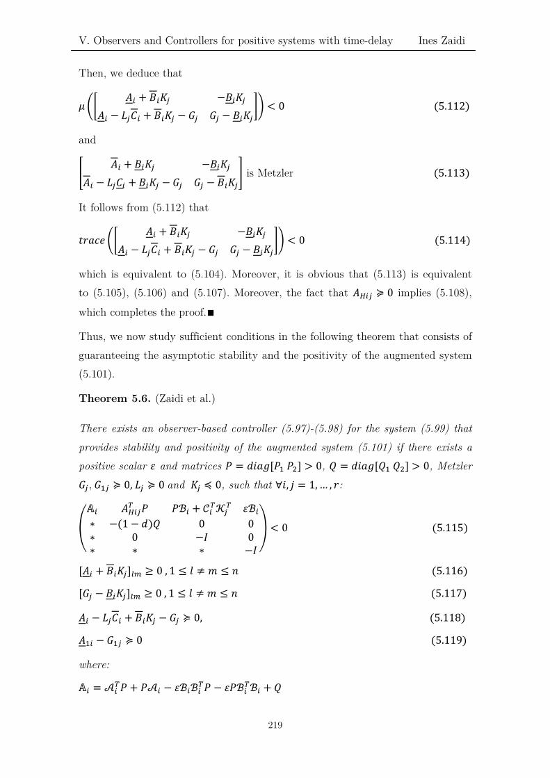
V. Observers and Controllers for positive systems with time-delay Ines Zaidi
Then, we deduce that
𝜇𝜇 ��𝐴𝐴𝑚𝑚 + 𝐵𝐵𝑚𝑚𝐾𝐾𝑖𝑖 −𝐵𝐵𝑚𝑚𝐾𝐾𝑖𝑖
𝐴𝐴𝑚𝑚 − 𝐿𝐿𝑖𝑖𝐶𝐶𝑚𝑚 + 𝐵𝐵𝑚𝑚𝐾𝐾𝑖𝑖 − 𝐺𝐺𝑖𝑖 𝐺𝐺𝑖𝑖 − 𝐵𝐵𝑚𝑚𝐾𝐾𝑖𝑖�� < 0 (5.112)
and
�𝐴𝐴𝑚𝑚 + 𝐵𝐵𝑚𝑚𝐾𝐾𝑖𝑖 −𝐵𝐵𝑚𝑚𝐾𝐾𝑖𝑖
𝐴𝐴𝑚𝑚 − 𝐿𝐿𝑖𝑖𝐶𝐶𝑚𝑚 + 𝐵𝐵𝑚𝑚𝐾𝐾𝑖𝑖 − 𝐺𝐺𝑖𝑖 𝐺𝐺𝑖𝑖 − 𝐵𝐵𝑚𝑚𝐾𝐾𝑖𝑖� is Metzler (5.113)
It follows from (5.112) that
𝑡𝑡𝑟𝑟𝑑𝑑𝑐𝑐𝑒𝑒 ��𝐴𝐴𝑚𝑚 + 𝐵𝐵𝑚𝑚𝐾𝐾𝑖𝑖 −𝐵𝐵𝑚𝑚𝐾𝐾𝑖𝑖
𝐴𝐴𝑚𝑚 − 𝐿𝐿𝑖𝑖𝐶𝐶𝑚𝑚 + 𝐵𝐵𝑚𝑚𝐾𝐾𝑖𝑖 − 𝐺𝐺𝑖𝑖 𝐺𝐺𝑖𝑖 − 𝐵𝐵𝑚𝑚𝐾𝐾𝑖𝑖�� < 0 (5.114)
which is equivalent to (5.104). Moreover, it is obvious that (5.113) is equivalent to (5.105), (5.106) and (5.107). Moreover, the fact that 𝐴𝐴𝐻𝐻𝑚𝑚𝑖𝑖 ≽ 0 implies (5.108),
which completes the proof.∎
Thus, we now study sufficient conditions in the following theorem that consists of guaranteeing the asymptotic stability and the positivity of the augmented system (5.101).
Theorem 5.6. (Zaidi et al.)
There exists an observer-based controller (5.97)-(5.98) for the system (5.99) that provides stability and positivity of the augmented system (5.101) if there exists a positive scalar 𝜀𝜀 and matrices 𝑃𝑃 = 𝑑𝑑𝑖𝑖𝑑𝑑𝑑𝑑[𝑃𝑃1 𝑃𝑃2] > 0, 𝑄𝑄 = 𝑑𝑑𝑖𝑖𝑑𝑑𝑑𝑑[𝑄𝑄1 𝑄𝑄2] > 0, Metzler 𝐺𝐺𝑖𝑖, 𝐺𝐺1𝑖𝑖 ≽ 0, 𝐿𝐿𝑖𝑖 ≽ 0 and 𝐾𝐾𝑖𝑖 ≼ 0, such that ∀𝑖𝑖, 𝑗𝑗 = 1, … , 𝑟𝑟:
�
𝔸𝔸𝑚𝑚 𝐴𝐴𝐻𝐻𝑚𝑚𝑖𝑖𝑇𝑇 𝑃𝑃 𝑃𝑃ℬ𝑚𝑚 + 𝒞𝒞𝑚𝑚
𝑇𝑇𝒦𝒦𝑖𝑖𝑇𝑇 𝜀𝜀ℬ𝑚𝑚
∗ −(1 − 𝑑𝑑)𝑄𝑄 0 0∗ 0 −𝐼𝐼 0∗ ∗ ∗ −𝐼𝐼
� < 0 (5.115)
[𝐴𝐴𝑚𝑚 + 𝐵𝐵𝑚𝑚𝐾𝐾𝑖𝑖]𝑘𝑘𝑚𝑚 ≥ 0 , 1 ≤ 𝑙𝑙 ≠ 𝐼𝐼 ≤ 𝑛𝑛 (5.116)
[𝐺𝐺𝑖𝑖 − 𝐵𝐵𝑚𝑚𝐾𝐾𝑖𝑖]𝑘𝑘𝑚𝑚 ≥ 0 , 1 ≤ 𝑙𝑙 ≠ 𝐼𝐼 ≤ 𝑛𝑛 (5.117)
𝐴𝐴𝑚𝑚 − 𝐿𝐿𝑖𝑖𝐶𝐶𝑚𝑚 + 𝐵𝐵𝑚𝑚𝐾𝐾𝑖𝑖 − 𝐺𝐺𝑖𝑖 ≽ 0, (5.118)
𝐴𝐴1𝑚𝑚 − 𝐺𝐺1𝑖𝑖 ≽ 0 (5.119)
where:
𝔸𝔸𝑚𝑚 = 𝒜𝒜𝑚𝑚𝑇𝑇𝑃𝑃 + 𝑃𝑃𝒜𝒜𝑚𝑚 − 𝜀𝜀ℬ𝑚𝑚ℬ𝑚𝑚
𝑇𝑇𝑃𝑃 − 𝜀𝜀𝑃𝑃ℬ𝑚𝑚𝑇𝑇ℬ𝑚𝑚 + 𝑄𝑄
219

V. Observers and Controllers for positive systems with time-delay Ines Zaidi
𝒜𝒜𝑚𝑚 = �𝐴𝐴𝑚𝑚 0𝐴𝐴𝑚𝑚 0
� , ℬ𝑚𝑚 = �0 𝐵𝐵𝑚𝑚 − 𝐵𝐵𝑚𝑚 0 𝐵𝐵𝑚𝑚
0 𝐵𝐵𝑚𝑚 − 𝐵𝐵𝑚𝑚 −𝐼𝐼 𝐵𝐵𝑚𝑚�
𝒦𝒦𝑖𝑖 =
⎝
⎜⎛
𝐺𝐺𝑖𝑖 𝐿𝐿𝑖𝑖 0 0𝐾𝐾𝑖𝑖 0 0 00 0 𝐺𝐺𝑖𝑖 𝐿𝐿𝑖𝑖0 0 𝐾𝐾𝑖𝑖 0 ⎠
⎟⎞
, 𝒞𝒞𝑚𝑚 = �
0 𝐼𝐼0 0𝐼𝐼 −𝐼𝐼
𝐶𝐶𝑚𝑚 0� (5.120)
Proof:
It follows from (5.116) that ∀𝑖𝑖, 𝑗𝑗 = 1, … , 𝑟𝑟, 𝐴𝐴𝑚𝑚 + 𝐵𝐵𝑚𝑚𝐾𝐾𝑖𝑖 is Metzler. Combining this
with 𝐾𝐾𝑖𝑖 ≼ 0 and 𝐿𝐿𝑖𝑖 ≽ 0 yields, for any 𝐴𝐴𝑚𝑚 ∈ [𝐴𝐴𝑚𝑚 , 𝐴𝐴𝑚𝑚], 𝐵𝐵𝑚𝑚 ∈ [𝐵𝐵𝑚𝑚 , 𝐵𝐵𝑚𝑚] and 𝐶𝐶𝑚𝑚 ∈
[𝐶𝐶𝑚𝑚 , 𝐶𝐶𝑚𝑚], we get: 𝐴𝐴𝑚𝑚 + 𝐵𝐵𝑚𝑚𝐾𝐾𝑖𝑖 ≽ 𝐴𝐴𝑚𝑚 + 𝐵𝐵𝑚𝑚𝐾𝐾𝑖𝑖 is Metzler (5.121)
and 𝐴𝐴𝑚𝑚 − 𝐿𝐿𝑖𝑖𝐶𝐶𝑚𝑚 + 𝐵𝐵𝑚𝑚 𝐾𝐾𝑖𝑖 − 𝐺𝐺𝑖𝑖 ≽ 𝐴𝐴𝑚𝑚 − 𝐿𝐿𝑖𝑖𝐶𝐶𝑚𝑚 + 𝐵𝐵𝑚𝑚𝐾𝐾𝑖𝑖 − 𝐺𝐺𝑖𝑖 ≽ 0 (5.122)
In addition, from 𝐺𝐺𝑖𝑖 being Metzler and 𝐾𝐾𝑖𝑖 ≼ 0 , we obtain that, for any
𝐵𝐵𝑚𝑚 ∈ [𝐵𝐵𝑚𝑚 , 𝐵𝐵𝑚𝑚]: −𝐵𝐵𝑚𝑚 𝐾𝐾𝑖𝑖 ≽ 0 (5.123)
and 𝐺𝐺𝑖𝑖 − 𝐵𝐵𝑚𝑚 𝐾𝐾𝑖𝑖 is Metzler (5.124)
Therefore, from (6.121)-(5.124) and the fact that 𝐴𝐴𝐻𝐻𝑚𝑚𝑖𝑖 ≽ 0, we have that, for any
𝐴𝐴𝑚𝑚 ∈ [𝐴𝐴𝑚𝑚 , 𝐴𝐴𝑚𝑚], 𝐴𝐴1𝑚𝑚 ∈ �𝐴𝐴1𝑚𝑚 , 𝐴𝐴1𝑚𝑚�, 𝐵𝐵𝑚𝑚 ∈ [𝐵𝐵𝑚𝑚 , 𝐵𝐵𝑚𝑚] and 𝐶𝐶𝑚𝑚 ∈ [𝐶𝐶𝑚𝑚 , 𝐶𝐶𝑚𝑚], the augmented
system (5.101) is positive.
It follows from (5.115), by the Schur complement, that:
�ℵ𝑚𝑚𝑖𝑖 𝐴𝐴𝐻𝐻𝑚𝑚𝑖𝑖
𝑇𝑇 𝑃𝑃∗ −(1 − 𝑑𝑑)𝑄𝑄
� < 0 (5.125)
where:
ℵ𝑚𝑚𝑖𝑖 = 𝒜𝒜𝑚𝑚𝑇𝑇𝑃𝑃 + 𝑃𝑃𝒜𝒜𝑚𝑚 − 𝜀𝜀ℬ𝑚𝑚ℬ𝑚𝑚
𝑇𝑇𝑃𝑃 − 𝜀𝜀𝑃𝑃ℬ𝑚𝑚𝑇𝑇ℬ𝑚𝑚 + 𝜀𝜀2ℬ𝑚𝑚ℬ𝑚𝑚
𝑇𝑇 + �ℬ𝑚𝑚𝑇𝑇𝑃𝑃 + 𝒦𝒦𝑖𝑖 𝒞𝒞𝑚𝑚�
𝑇𝑇�ℬ𝑚𝑚
𝑇𝑇𝑃𝑃 + 𝒦𝒦𝑖𝑖 𝒞𝒞𝑚𝑚�
+𝑄𝑄
We have then:
𝒜𝒜𝑚𝑚𝑇𝑇𝑃𝑃 + 𝑃𝑃𝒜𝒜𝑚𝑚 − 𝜀𝜀ℬ𝑚𝑚ℬ𝑚𝑚
𝑇𝑇𝑃𝑃 − 𝜀𝜀𝑃𝑃ℬ𝑚𝑚𝑇𝑇ℬ𝑚𝑚 + 𝜀𝜀2ℬ𝑚𝑚ℬ𝑚𝑚
𝑇𝑇 + �ℬ𝑚𝑚𝑇𝑇𝑃𝑃 + 𝒦𝒦𝑖𝑖 𝒞𝒞𝑚𝑚�
𝑇𝑇�ℬ𝑚𝑚
𝑇𝑇𝑃𝑃 + 𝒦𝒦𝑖𝑖 𝒞𝒞𝑚𝑚�
+𝑄𝑄 < 0 (5.126)
Taking into account the following relationship:
𝑃𝑃ℬ𝑚𝑚ℬ𝑚𝑚𝑇𝑇𝑃𝑃 − 𝜀𝜀ℬ𝑚𝑚ℬ𝑚𝑚
𝑇𝑇𝑃𝑃 − 𝜀𝜀𝑃𝑃ℬ𝑚𝑚𝑇𝑇ℬ𝑚𝑚 + 𝜀𝜀2ℬ𝑚𝑚ℬ𝑚𝑚
𝑇𝑇 = (𝑃𝑃ℬ𝑚𝑚 −𝜀𝜀 ℬ𝑚𝑚)(ℬ𝑚𝑚𝑇𝑇𝑃𝑃 − 𝜀𝜀 ℬ𝑚𝑚
𝑇𝑇) ≥ 0 (5.127)
we obtain the following inequality:
220

V. Observers and Controllers for positive systems with time-delay Ines Zaidi
𝒜𝒜𝑚𝑚𝑇𝑇𝑃𝑃 + 𝑃𝑃𝒜𝒜𝑚𝑚 − 𝑃𝑃ℬ𝑚𝑚ℬ𝑚𝑚
𝑇𝑇𝑃𝑃 + �ℬ𝑚𝑚𝑇𝑇𝑃𝑃 + 𝒦𝒦𝑖𝑖 𝒞𝒞𝑚𝑚�
𝑇𝑇�ℬ𝑚𝑚
𝑇𝑇𝑃𝑃 + 𝒦𝒦𝑖𝑖 𝒞𝒞𝑚𝑚� + 𝑄𝑄 < 0 (5.128)
Rewriting (5.128) yields that:
(𝒜𝒜𝑚𝑚 + ℬ𝑚𝑚𝒦𝒦𝑖𝑖 𝒞𝒞𝑚𝑚)𝑇𝑇𝑃𝑃 + 𝑃𝑃�𝒜𝒜𝑚𝑚 + ℬ𝑚𝑚𝒦𝒦𝑖𝑖 𝒞𝒞𝑚𝑚� + 𝒞𝒞𝑚𝑚𝑇𝑇𝒦𝒦𝐽𝐽
𝑇𝑇𝒦𝒦𝑖𝑖 𝒞𝒞𝑚𝑚 + 𝑄𝑄 < 0 (5.129)
which implies that:
(𝒜𝒜𝑚𝑚 + ℬ𝑚𝑚𝒦𝒦𝑖𝑖 𝒞𝒞𝑚𝑚)𝑇𝑇𝑃𝑃 + 𝑃𝑃�𝒜𝒜𝑚𝑚 + ℬ𝑚𝑚𝒦𝒦𝑖𝑖 𝒞𝒞𝑚𝑚� + 𝑄𝑄 < 0 (5.128)
Therefore, we get: 𝜇𝜇�𝒜𝒜𝑚𝑚 + ℬ𝑚𝑚𝒦𝒦𝑖𝑖 𝒞𝒞𝑚𝑚� < 0 (5.129)
Replacing ℵ𝑚𝑚𝑖𝑖 with (5.1128) in (5.125), we get:
��𝒜𝒜𝑚𝑚 + ℬ𝑚𝑚𝒦𝒦𝑖𝑖 𝒞𝒞𝑚𝑚�𝑇𝑇
𝑃𝑃 + 𝑃𝑃�𝒜𝒜𝑚𝑚 + ℬ𝑚𝑚𝒦𝒦𝑖𝑖 𝒞𝒞𝑚𝑚� + 𝑄𝑄 ∗𝑃𝑃𝐴𝐴𝐻𝐻𝑚𝑚𝑖𝑖 −(1 − 𝑑𝑑)𝑄𝑄
� < 0 (5.130)
Some algebraic manipulations lead to:
𝒜𝒜𝑚𝑚 + ℬ𝑚𝑚𝒦𝒦𝑖𝑖 𝒞𝒞𝑚𝑚 = �𝐴𝐴𝑚𝑚 + 𝐵𝐵𝑚𝑚𝐾𝐾𝑖𝑖 −𝐵𝐵𝑚𝑚𝐾𝐾𝑖𝑖
𝐴𝐴𝑚𝑚 − 𝐿𝐿𝑖𝑖𝐶𝐶𝑚𝑚 + 𝐵𝐵𝑚𝑚𝐾𝐾𝑖𝑖 − 𝐺𝐺𝑖𝑖 𝐺𝐺𝑖𝑖 − 𝐵𝐵𝑚𝑚𝐾𝐾𝑖𝑖� (5.131)
In addition, it is easy to show that:
�𝐴𝐴𝑚𝑚 + 𝐵𝐵𝑚𝑚𝐾𝐾𝑖𝑖 −𝐵𝐵𝑚𝑚𝐾𝐾𝑖𝑖
𝐴𝐴𝑚𝑚 − 𝐿𝐿𝑖𝑖𝐶𝐶𝑚𝑚 + 𝐵𝐵𝑚𝑚𝐾𝐾𝑖𝑖 − 𝐺𝐺𝑖𝑖 𝐺𝐺𝑖𝑖 − 𝐵𝐵𝑚𝑚𝐾𝐾𝑖𝑖� ≽ �
𝐴𝐴𝑚𝑚 + 𝐵𝐵𝑚𝑚𝐾𝐾𝑖𝑖 −𝐵𝐵𝑚𝑚𝐾𝐾𝑖𝑖𝐴𝐴𝑚𝑚 − 𝐿𝐿𝑖𝑖𝐶𝐶𝑚𝑚 + 𝐵𝐵𝑚𝑚 𝐾𝐾𝑖𝑖 − 𝐺𝐺𝑖𝑖 𝐺𝐺𝑖𝑖 − 𝐵𝐵𝑚𝑚 𝐾𝐾𝑖𝑖
� (5.132)
Therefore, by combining (5.130)-(5.132) and using Lemma 3.1, we obtain that:
𝜇𝜇 ��𝐴𝐴𝑚𝑚 + 𝐵𝐵𝑚𝑚𝐾𝐾𝑖𝑖 −𝐵𝐵𝑚𝑚𝐾𝐾𝑖𝑖
𝐴𝐴𝑚𝑚 − 𝐿𝐿𝑖𝑖𝐶𝐶𝑚𝑚 + 𝐵𝐵𝑚𝑚 𝐾𝐾𝑖𝑖 − 𝐺𝐺𝑖𝑖 𝐺𝐺𝑖𝑖 − 𝐵𝐵𝑚𝑚 𝐾𝐾𝑖𝑖�� < 0 (5.132)
which means that (5.101) is asymptotically stable for any 𝐴𝐴𝑚𝑚 ∈ [𝐴𝐴𝑚𝑚 , 𝐴𝐴𝑚𝑚], 𝐵𝐵𝑚𝑚 ∈
[𝐵𝐵𝑚𝑚 , 𝐵𝐵𝑚𝑚] and 𝐶𝐶𝑚𝑚 ∈ [𝐶𝐶𝑚𝑚 , 𝐶𝐶𝑚𝑚].
This completes the proof.∎
5.4.2. CASE 2: UNMEASURABLE PREMISE VARIABLES
We consider the observer design for the following positive interval time-delay T-S system (5.91) with unmeasurable premise variables
⎩⎪⎪⎨
⎪⎪⎧�̇�𝑥(𝑡𝑡) = � ℎ𝑚𝑚(𝑥𝑥(𝑡𝑡))(𝐴𝐴𝑚𝑚𝑥𝑥(𝑡𝑡) + 𝐴𝐴1𝑚𝑚𝑥𝑥�𝑡𝑡 − 𝜏𝜏𝑚𝑚(𝑡𝑡)� + 𝐵𝐵𝑚𝑚𝑢𝑢(𝑡𝑡))
𝑟𝑟
𝑚𝑚=1
𝑦𝑦(𝑡𝑡) = � ℎ𝑚𝑚(𝑥𝑥(𝑡𝑡))𝑟𝑟
𝑚𝑚=1
𝐶𝐶𝑚𝑚 𝑥𝑥(𝑡𝑡)
𝑥𝑥(𝑡𝑡) = 𝜑𝜑(𝑡𝑡) ≽ 0, ∀ 𝑡𝑡 ∈ �−ℎ, 0�
(5.133)
221

V. Observers and Controllers for positive systems with time-delay Ines Zaidi
where ℎ𝑚𝑚(𝑥𝑥(𝑡𝑡)) are fuzzy weighting functions that depend on the state of the system and satisfy (1.4)
Remark 5.1.
In order to simplify the mathematical notations, we consider a single delay in the model. However, the proposed technique can be easily generalized to systems with multiple delays (Following, for example, (Rami & Tadeo, 2007)).
Taking into account that the state is estimated, the T-S model with unmeasurable variables (5.91) can be reduced to (Zaidi et al, 2013c):
⎩⎪⎪⎨
⎪⎪⎧ �̇�𝑥(𝑡𝑡) = � ℎ𝑚𝑚�𝑥𝑥�(𝑡𝑡)�
𝑟𝑟
𝑚𝑚=1
(𝐴𝐴𝑚𝑚𝑥𝑥�(𝑡𝑡) + 𝐵𝐵𝑚𝑚 𝑢𝑢(𝑡𝑡)) + 𝑤𝑤(𝑡𝑡)
𝑦𝑦(𝑡𝑡) = � ℎ𝑚𝑚(𝑥𝑥(𝑡𝑡))𝑟𝑟
𝑚𝑚=1
𝐶𝐶𝑚𝑚 𝑥𝑥(𝑡𝑡)
𝑥𝑥(𝑡𝑡) = 𝜑𝜑(𝑡𝑡) ≽ 0, ∀ 𝑡𝑡 ∈ �−ℎ, 0�
(5.134)
where :
𝑤𝑤(𝑡𝑡) = �(𝑟𝑟
𝑚𝑚=1
ℎ𝑚𝑚�𝑥𝑥(𝑡𝑡)� − ℎ𝑚𝑚�𝑥𝑥�(𝑡𝑡)�) (𝐴𝐴𝑚𝑚𝑥𝑥(𝑡𝑡) + 𝐵𝐵𝑚𝑚𝑢𝑢(𝑡𝑡)) (5.135)
Using Lemma 2.4, we have :
��ℎ𝑚𝑚(𝑥𝑥) − ℎ𝑚𝑚(𝑥𝑥�)�𝑋𝑋𝑚𝑚 = � ℎ𝑚𝑚(𝑥𝑥)ℎ𝑖𝑖(𝑥𝑥�)∆𝑋𝑋𝑚𝑚𝑖𝑖
𝑟𝑟
𝑚𝑚,𝑖𝑖=1
𝑟𝑟
𝑚𝑚=1
(5.136)
where 𝑋𝑋𝑚𝑚 є {𝐴𝐴𝑚𝑚 , 𝐴𝐴1𝑚𝑚, 𝐵𝐵𝑚𝑚} and ∆𝑋𝑋𝑚𝑚𝑖𝑖 is defined by:
∆𝑋𝑋𝑚𝑚𝑖𝑖 = 𝑋𝑋𝑚𝑚 − 𝑋𝑋𝑖𝑖 (5.137)
System (5.134) can then be transformed into the following system (Zaidi et al, 2013c):
⎩⎪⎪⎨
⎪⎪⎧�̇�𝑥(𝑡𝑡) = � ℎ𝑚𝑚�𝑥𝑥(𝑡𝑡)�ℎ𝑖𝑖�𝑥𝑥�(𝑡𝑡)� ��𝐴𝐴𝑚𝑚 + ∆𝐴𝐴𝑚𝑚𝑖𝑖�𝑥𝑥(𝑡𝑡) + (𝐴𝐴1𝑚𝑚 + ∆𝐴𝐴1𝑚𝑚𝑖𝑖)𝑥𝑥�𝑡𝑡 − 𝜏𝜏𝑚𝑚(𝑡𝑡)� + (𝐵𝐵𝑚𝑚 + ∆𝐵𝐵𝑚𝑚𝑖𝑖)𝑢𝑢(𝑡𝑡)�
𝑟𝑟
𝑚𝑚,𝑖𝑖=1
𝑦𝑦(𝑡𝑡) = � ℎ𝑚𝑚(𝑥𝑥(𝑡𝑡))𝑟𝑟
𝑚𝑚=1
𝐶𝐶𝑚𝑚 𝑥𝑥(𝑡𝑡)
𝑥𝑥(𝑡𝑡) = 𝜑𝜑(𝑡𝑡) ≽ 0, ∀ 𝑡𝑡 ∈ �−ℎ, 0�
(5.138)
222

V. Observers and Controllers for positive systems with time-delay Ines Zaidi
where: ∆𝑋𝑋𝑚𝑚𝑖𝑖 = 𝑋𝑋𝑚𝑚 − 𝑋𝑋𝑖𝑖, with 𝑋𝑋𝑚𝑚 = {𝐴𝐴𝑚𝑚 , 𝐴𝐴1𝑚𝑚, 𝐵𝐵𝑚𝑚}.
The overall observer-based controller under consideration has the following form:
𝑥𝑥�̇(𝑡𝑡) = � ℎ𝑚𝑚(𝑥𝑥�(𝑡𝑡))(𝐺𝐺𝑚𝑚 𝑥𝑥�(𝑡𝑡) + 𝐺𝐺1𝑚𝑚 𝑥𝑥��𝑡𝑡 − 𝜏𝜏(𝑡𝑡)� + 𝐿𝐿𝑚𝑚𝑦𝑦(𝑡𝑡))𝑟𝑟
𝑚𝑚=1
(5.139)
where 𝐺𝐺𝑚𝑚 ∈ ℝ𝑛𝑛𝑥𝑥×𝑛𝑛𝑥𝑥 , 𝐺𝐺1𝑚𝑚 ∈ ℝ𝑛𝑛𝑥𝑥×𝑛𝑛𝑥𝑥, 𝐿𝐿𝑚𝑚 ∈ ℝ𝑛𝑛𝑥𝑥×𝑛𝑛𝑦𝑦 and 𝐾𝐾𝑚𝑚 ∈ ℝ𝑛𝑛𝑢𝑢×𝑛𝑛𝑥𝑥, ∀ 𝑖𝑖 = 1, … , 𝑟𝑟, are the observer matrices to be determined.
The static state-feedback control law is given by the following expression:
𝑢𝑢(𝑡𝑡) = � ℎ𝑚𝑚�𝑥𝑥�(𝑡𝑡)�𝐾𝐾𝑚𝑚𝑥𝑥�(𝑡𝑡)𝑟𝑟
𝑚𝑚=1
(5.140)
where 𝐾𝐾𝑚𝑚 ∈ ℝ𝑛𝑛𝑢𝑢×𝑛𝑛𝑥𝑥 are the controller matrices to be determined.
Then, the closed-loop system is written as follows:
⎩⎪⎪⎪⎨
⎪⎪⎪⎧�̇�𝑥(𝑡𝑡) = � ℎ𝑚𝑚(𝑥𝑥)ℎ𝑖𝑖(𝑥𝑥�)ℎ𝑘𝑘(𝑥𝑥�) ��𝐴𝐴𝑚𝑚 + ∆𝐴𝐴𝑚𝑚𝑖𝑖�𝑥𝑥(𝑡𝑡) + (𝐴𝐴1𝑚𝑚 + ∆𝐴𝐴1𝑚𝑚𝑖𝑖)𝑥𝑥�𝑡𝑡 − 𝜏𝜏𝑚𝑚(𝑡𝑡)� + (𝐵𝐵 + ∆𝐵𝐵𝑚𝑚𝑖𝑖)𝐾𝐾𝑘𝑘𝑥𝑥�(𝑡𝑡)�
𝑟𝑟
𝑚𝑚,𝑖𝑖,𝑘𝑘=1
𝑦𝑦(𝑡𝑡) = � ℎ𝑚𝑚(𝑥𝑥(𝑡𝑡))𝑟𝑟
𝑚𝑚=1
𝐶𝐶𝑚𝑚 𝑥𝑥(𝑡𝑡)
𝑥𝑥(𝑡𝑡) = 𝜑𝜑(𝑡𝑡) ≽ 0, ∀ 𝑡𝑡 ∈ �−ℎ, 0� 𝑥𝑥�(𝑡𝑡) = 𝜗𝜗(𝑡𝑡) ≽ 0, ∀ 𝑡𝑡 ∈ �−ℎ, 0�
(5.141)
The key lies in the error, which is defined by:
𝑒𝑒(𝑡𝑡) = 𝑥𝑥(𝑡𝑡) − 𝑥𝑥�(𝑡𝑡). (5.142)
If we choose [𝑥𝑥𝑇𝑇(𝑡𝑡) 𝑒𝑒𝑇𝑇(𝑡𝑡)]𝑇𝑇 as the new augmented state variable, then the new closed-loop system will become:
��̇�𝑥(𝑡𝑡)�̇�𝑒(𝑡𝑡)
� = � ℎ𝑚𝑚�𝑥𝑥(𝑡𝑡)�𝑟𝑟
𝑚𝑚,𝑖𝑖,𝑘𝑘=1
ℎ𝑖𝑖�𝑥𝑥�(𝑡𝑡)�ℎ𝑘𝑘�𝑥𝑥�(𝑡𝑡)� �𝐴𝐴𝑋𝑋𝑚𝑚𝑖𝑖𝑘𝑘 �𝑥𝑥(𝑡𝑡)
𝑒𝑒(𝑡𝑡)� + 𝐴𝐴𝐻𝐻𝑚𝑚𝑖𝑖 �
𝑥𝑥(𝑡𝑡 − ℎ(𝑡𝑡)𝑒𝑒�𝑡𝑡 − ℎ(𝑡𝑡)���
(5.143)
where:
𝐴𝐴𝑋𝑋𝑚𝑚𝑖𝑖𝑘𝑘 = �
𝐴𝐴𝑚𝑚 + ∆𝐴𝐴𝑚𝑚𝑖𝑖 + (𝐵𝐵𝑚𝑚 + ∆𝐵𝐵𝑚𝑚𝑖𝑖)𝐾𝐾𝑘𝑘 −(𝐵𝐵𝑚𝑚 + ∆𝐵𝐵𝑚𝑚𝑖𝑖)𝐾𝐾𝑘𝑘𝐴𝐴𝑚𝑚 + ∆𝐴𝐴𝑚𝑚𝑖𝑖 − 𝐿𝐿𝑖𝑖𝐶𝐶𝑚𝑚 + (𝐵𝐵𝑚𝑚 + ∆𝐵𝐵𝑚𝑚𝑖𝑖)𝐾𝐾𝑘𝑘 − 𝐺𝐺𝑖𝑖 𝐺𝐺𝑖𝑖 − (𝐵𝐵𝑚𝑚 + ∆𝐵𝐵𝑚𝑚𝑖𝑖)𝐾𝐾𝑘𝑘
�
and
223

V. Observers and Controllers for positive systems with time-delay Ines Zaidi
𝐴𝐴𝐻𝐻𝑚𝑚𝑖𝑖 = �
𝐴𝐴1𝑚𝑚 + ∆𝐴𝐴1𝑚𝑚𝑖𝑖 0𝐴𝐴1𝑚𝑚 + ∆𝐴𝐴1𝑚𝑚𝑖𝑖 − 𝐺𝐺1𝑖𝑖 𝐺𝐺1𝑖𝑖
�
The following theorem provides necessary conditions for the existence of an observer-based controller (5.139) for positive time-delay T-S systems with unmeasurable premise variables.
Theorem 5.7. (Zaidi et al.)
For a given interval positive closed-loop T-S system in (5.141), if there exist diagonal matrices 𝑋𝑋1, 𝑋𝑋2, 𝑄𝑄1 and 𝑄𝑄2, matrices 𝑊𝑊1𝑖𝑖, 𝑊𝑊2𝑖𝑖, 𝑊𝑊11𝑖𝑖, 𝑊𝑊12𝑖𝑖, 𝐿𝐿𝑚𝑚, 𝐾𝐾𝑘𝑘,
∀ 𝑖𝑖, 𝑗𝑗, 𝑟𝑟 = 1, … , 𝑟𝑟 and a scalar 𝛾𝛾 > 0 such that :
⎝
⎜⎛
𝑆𝑆𝑚𝑚𝑖𝑖𝑘𝑘 𝑇𝑇𝑚𝑚𝑖𝑖𝑘𝑘 (𝐴𝐴1𝑚𝑚 + ∆𝐴𝐴1𝑚𝑚𝑖𝑖)𝑋𝑋1 0∗ 𝑈𝑈𝑚𝑚𝑖𝑖𝑘𝑘 �𝐴𝐴1𝑚𝑚 + ∆𝐴𝐴1𝑚𝑚𝑖𝑖�𝑋𝑋1 − 𝑊𝑊11𝑖𝑖 𝑊𝑊12𝑖𝑖∗ ∗ −(1 − 𝑑𝑑)𝑅𝑅1 0∗ ∗ ∗ −(1 − 𝑑𝑑)𝑅𝑅2⎠
⎟⎞
< 0 (5.144)
and
�𝐿𝐿𝑚𝑚𝑖𝑖𝑘𝑘 𝑀𝑀𝑚𝑚𝑖𝑖𝑘𝑘𝑁𝑁𝑚𝑚𝑖𝑖𝑘𝑘 𝑂𝑂𝑚𝑚𝑖𝑖𝑘𝑘
� ≽ 0 (5.145)
where:
𝑆𝑆𝑚𝑚𝑖𝑖𝑘𝑘 = (𝐴𝐴𝑚𝑚 + ∆𝐴𝐴𝑚𝑚𝑖𝑖)𝑋𝑋1 + 𝑋𝑋1(𝐴𝐴𝑚𝑚 + ∆𝐴𝐴𝑚𝑚𝑖𝑖)𝑇𝑇 + (𝐵𝐵𝑚𝑚 + ∆𝐵𝐵𝑚𝑚𝑖𝑖)𝑌𝑌1𝑘𝑘 + 𝑌𝑌1𝑘𝑘𝑇𝑇(𝐵𝐵𝑚𝑚 + ∆𝐵𝐵𝑚𝑚𝑖𝑖)𝑇𝑇 + 𝑅𝑅1
𝑇𝑇𝑚𝑚𝑖𝑖𝑘𝑘 = 𝑋𝑋1(𝐴𝐴𝑚𝑚 + ∆𝐴𝐴𝑚𝑚𝑖𝑖)𝑇𝑇 − (𝐵𝐵𝑚𝑚 + ∆𝐵𝐵𝑚𝑚𝑖𝑖)𝑌𝑌2𝑘𝑘 − 𝐶𝐶𝑚𝑚𝑇𝑇𝑍𝑍𝑖𝑖
𝑇𝑇 + 𝑌𝑌1𝑘𝑘𝑇𝑇(𝐵𝐵𝑚𝑚 + ∆𝐵𝐵𝑚𝑚𝑖𝑖)𝑇𝑇 − 𝑊𝑊1𝑖𝑖
𝑇𝑇
𝑈𝑈𝑚𝑚𝑖𝑖𝑘𝑘 = −�𝐵𝐵𝑚𝑚 + ∆𝐵𝐵𝑚𝑚𝑖𝑖�𝑌𝑌2𝑘𝑘 − 𝑌𝑌2𝑘𝑘𝑇𝑇�𝐵𝐵𝑚𝑚 + ∆𝐵𝐵𝑚𝑚𝑖𝑖�
𝑇𝑇+ 𝑊𝑊2𝑖𝑖
𝑇𝑇 + 𝑅𝑅1
𝐿𝐿𝑚𝑚𝑖𝑖𝑘𝑘 = (𝐴𝐴𝑚𝑚 + ∆𝐴𝐴𝑚𝑚𝑖𝑖)𝑋𝑋1 + (𝐵𝐵𝑚𝑚 + ∆𝐵𝐵𝑚𝑚𝑖𝑖)𝑌𝑌1𝑘𝑘 + 𝛾𝛾𝑋𝑋1
𝑀𝑀𝑚𝑚𝑖𝑖𝑘𝑘 = −(𝐵𝐵𝑚𝑚 + ∆𝐵𝐵𝑚𝑚𝑖𝑖)𝑌𝑌2𝑘𝑘
𝑁𝑁𝑚𝑚𝑖𝑖𝑘𝑘 = (𝐴𝐴𝑚𝑚 + ∆𝐴𝐴𝑚𝑚𝑖𝑖)𝑋𝑋1 − 𝑍𝑍𝑖𝑖𝐶𝐶𝑚𝑚 + (𝐵𝐵𝑚𝑚 + ∆𝐵𝐵𝑚𝑚𝑖𝑖)𝑌𝑌1𝑘𝑘 − 𝑊𝑊1𝑖𝑖
𝑂𝑂𝑚𝑚𝑖𝑖𝑘𝑘 = 𝑊𝑊2𝑖𝑖 − (𝐵𝐵𝑚𝑚 + ∆𝐵𝐵𝑚𝑚𝑖𝑖)𝑌𝑌2𝑘𝑘 + 𝛾𝛾𝑋𝑋2
𝑋𝑋1 = 𝑃𝑃1−1, 𝑋𝑋2 = 𝑃𝑃2
−1, 𝑅𝑅1 = 𝑋𝑋1𝑄𝑄1−1𝑋𝑋1, 𝑅𝑅2 = 𝑋𝑋2𝑄𝑄2
−1𝑋𝑋2,
then, the augmented system (5.143) is asymptotically stable, while remaining positive.
Under these conditions, the desired observer and controller gain matrices may be obtained from
𝐾𝐾𝑘𝑘 = 𝑌𝑌1𝑘𝑘𝑋𝑋1−1, 𝐿𝐿𝑖𝑖 = 𝑍𝑍𝑖𝑖𝑉𝑉1
−1, 𝐺𝐺𝑖𝑖 = 𝑊𝑊1𝑖𝑖𝑋𝑋1−1, 𝐺𝐺1𝑖𝑖 = 𝑊𝑊11𝑖𝑖𝑋𝑋1
−1,
224

V. Observers and Controllers for positive systems with time-delay Ines Zaidi
where 𝑉𝑉1 fulfills 𝐶𝐶𝑚𝑚𝑋𝑋1 = 𝑉𝑉1𝐶𝐶𝑚𝑚.
Proof:
Assume that ∀ 𝑖𝑖, 𝑗𝑗, 𝑟𝑟 = 1, … , 𝑟𝑟, there exist, 𝐺𝐺𝑚𝑚, 𝐺𝐺1𝑚𝑚, 𝐿𝐿𝑚𝑚and 𝐾𝐾𝑘𝑘 such that (5.143) is positive and asymptotically stable, then, there exist diagonal matrices 𝑃𝑃 and 𝑄𝑄 in
the following forms 𝑃𝑃 = �𝑃𝑃1 00 𝑃𝑃2
� > 0 and 𝑄𝑄 = �𝑄𝑄1 00 𝑄𝑄2
� > 0 such that the
following LMIs hold :
�𝑃𝑃𝐴𝐴𝑋𝑋𝑚𝑚𝑖𝑖𝑘𝑘 + 𝐴𝐴𝑋𝑋
𝑚𝑚𝑖𝑖𝑘𝑘𝑇𝑇𝑃𝑃 + 𝑄𝑄 𝑃𝑃𝐴𝐴𝐻𝐻
𝑚𝑚𝑖𝑖
∗ −(1 − 𝑑𝑑)𝑄𝑄� < 0 (5.146)
Multiplying each LMI on the left by 𝑑𝑑𝑖𝑖𝑑𝑑𝑑𝑑(𝑃𝑃−1, 𝑃𝑃−1), we get:
�𝐴𝐴𝑋𝑋𝑚𝑚𝑖𝑖𝑘𝑘 + 𝑃𝑃−1𝐴𝐴𝑋𝑋
𝑚𝑚𝑖𝑖𝑘𝑘𝑇𝑇𝑃𝑃 + 𝑃𝑃−1𝑄𝑄 𝐴𝐴𝐻𝐻
𝑚𝑚𝑖𝑖
∗ −(1 − 𝑑𝑑)𝑃𝑃−1𝑄𝑄� < 0 (5.147)
Then, multiplying on the right by 𝑑𝑑𝑖𝑖𝑑𝑑𝑑𝑑(𝑃𝑃−1, 𝑃𝑃−1), we obtain:
�𝐴𝐴𝑋𝑋𝑚𝑚𝑖𝑖𝑘𝑘𝑃𝑃−1 + 𝑃𝑃−1𝐴𝐴𝑋𝑋
𝑚𝑚𝑖𝑖𝑘𝑘𝑇𝑇+ 𝑃𝑃−1𝑄𝑄𝑃𝑃−1 𝐴𝐴𝐻𝐻
𝑚𝑚𝑖𝑖𝑃𝑃−1
∗ −(1 − 𝑑𝑑)𝑃𝑃−1𝑄𝑄𝑃𝑃−1� < 0 (5.148)
Taking the following change of variables: 𝑋𝑋1 = 𝑃𝑃1−1, 𝑋𝑋2 = 𝑃𝑃2
−1, 𝑌𝑌1𝑘𝑘 =
𝐾𝐾𝑘𝑘𝑋𝑋1 , 𝑌𝑌2𝑘𝑘 = 𝐾𝐾𝑘𝑘𝑋𝑋2 and 𝑉𝑉1𝐶𝐶𝑚𝑚 = 𝐶𝐶𝑚𝑚𝑋𝑋1, leads to the following LMIs:
⎝
⎜⎛
𝑑𝑑𝑚𝑚𝑖𝑖𝑘𝑘 𝑏𝑏𝑚𝑚𝑖𝑖𝑘𝑘 (𝐴𝐴1𝑚𝑚 + ∆𝐴𝐴1𝑚𝑚𝑖𝑖)𝑋𝑋1 0∗ 𝑐𝑐𝑚𝑚𝑖𝑖𝑘𝑘 �𝐴𝐴1𝑚𝑚 + ∆𝐴𝐴1𝑚𝑚𝑖𝑖�𝑋𝑋1 − 𝐺𝐺1𝑖𝑖𝑋𝑋2 𝐺𝐺1𝑖𝑖𝑋𝑋2∗ ∗ −(1 − 𝑑𝑑)𝑋𝑋1𝑄𝑄1𝑋𝑋1 0∗ ∗ ∗ −(1 − 𝑑𝑑)𝑋𝑋2𝑄𝑄2𝑋𝑋2⎠
⎟⎞
< 0 (5.149)
where
𝑑𝑑𝑚𝑚𝑖𝑖𝑘𝑘 = (𝐴𝐴𝑚𝑚 + ∆𝐴𝐴𝑚𝑚𝑖𝑖)𝑋𝑋1 + 𝑋𝑋1(𝐴𝐴𝑚𝑚 + ∆𝐴𝐴𝑚𝑚𝑖𝑖)𝑇𝑇 + (𝐵𝐵𝑚𝑚 + ∆𝐵𝐵𝑚𝑚𝑖𝑖)𝑌𝑌1𝑘𝑘 + 𝑌𝑌1𝑘𝑘𝑇𝑇(𝐵𝐵𝑚𝑚 + ∆𝐵𝐵𝑚𝑚𝑖𝑖)𝑇𝑇
+𝑋𝑋1𝑄𝑄1𝑋𝑋1
𝑏𝑏𝑚𝑚𝑖𝑖𝑘𝑘 = 𝑋𝑋1(𝐴𝐴𝑚𝑚 + ∆𝐴𝐴𝑚𝑚𝑖𝑖)𝑇𝑇 − (𝐵𝐵𝑚𝑚 + ∆𝐵𝐵𝑚𝑚𝑖𝑖)𝑌𝑌2𝑘𝑘 − 𝐶𝐶𝑚𝑚𝑇𝑇𝑉𝑉1
𝑇𝑇𝐿𝐿𝑖𝑖𝑇𝑇 + 𝑌𝑌1𝑘𝑘
𝑇𝑇(𝐵𝐵𝑚𝑚 + ∆𝐵𝐵𝑚𝑚𝑖𝑖)𝑇𝑇 − 𝑋𝑋1𝐺𝐺𝑚𝑚𝑇𝑇
𝑐𝑐𝑚𝑚𝑖𝑖𝑘𝑘 = −�𝐵𝐵𝑚𝑚 + ∆𝐵𝐵𝑚𝑚𝑖𝑖�𝑌𝑌2 − 𝑌𝑌2𝑇𝑇�𝐵𝐵𝑚𝑚 + ∆𝐵𝐵𝑚𝑚𝑖𝑖�
𝑇𝑇+ 𝑋𝑋2𝐺𝐺𝑚𝑚
𝑇𝑇 + 𝑋𝑋2𝑄𝑄2𝑋𝑋2
∀ 𝑖𝑖, 𝑗𝑗, 𝑟𝑟 = 1, … , 𝑟𝑟.
Considering that 𝑍𝑍𝑖𝑖 = 𝐿𝐿𝑖𝑖𝑉𝑉1, 𝑊𝑊1𝑖𝑖 = 𝐺𝐺𝑖𝑖𝑋𝑋1, 𝑊𝑊2𝑖𝑖 = 𝐺𝐺𝑖𝑖𝑋𝑋2, 𝑊𝑊11𝑖𝑖 = 𝐺𝐺1𝑖𝑖𝑋𝑋1, 𝑊𝑊12𝑖𝑖 = 𝐺𝐺1𝑖𝑖 ,
𝑅𝑅1 = 𝑋𝑋1𝑄𝑄1𝑋𝑋1 and 𝑅𝑅2 = 𝑋𝑋2𝑄𝑄2𝑋𝑋2, we get:
225

V. Observers and Controllers for positive systems with time-delay Ines Zaidi
⎝
⎜⎛
𝑆𝑆𝑚𝑚𝑖𝑖𝑘𝑘 𝑇𝑇𝑚𝑚𝑖𝑖𝑘𝑘 (𝐴𝐴1𝑚𝑚 + ∆𝐴𝐴1𝑚𝑚𝑖𝑖)𝑋𝑋1 0∗ 𝑈𝑈𝑚𝑚𝑖𝑖𝑘𝑘 �𝐴𝐴1𝑚𝑚 + ∆𝐴𝐴1𝑚𝑚𝑖𝑖�𝑋𝑋1 − 𝑊𝑊11𝑖𝑖 𝑊𝑊12𝑖𝑖∗ ∗ −(1 − 𝑑𝑑)𝑅𝑅1 0∗ ∗ ∗ −(1 − 𝑑𝑑)𝑅𝑅2⎠
⎟⎞
< 0 (5.150)
In order to guarantee the positivity of the augmented system (5.143), we have to prove that all 𝐴𝐴𝑋𝑋
𝑚𝑚𝑖𝑖𝑘𝑘 are Metzler, or equivalently, that there exists a positive scalar
𝛾𝛾 such that 𝐴𝐴𝑋𝑋𝑚𝑚𝑖𝑖𝑘𝑘 + 𝛾𝛾𝐼𝐼 ≽ 0. Multiplying on the right by 𝑑𝑑𝑖𝑖𝑑𝑑𝑑𝑑(𝑋𝑋1, 𝑋𝑋2), we get
(5.145).
Once these LMIs are programmed and solved, we can obtain the observer and controller gain matrices:
𝐾𝐾𝑘𝑘 = 𝑌𝑌2𝑘𝑘𝑋𝑋2−1, 𝐿𝐿𝑖𝑖 = 𝑍𝑍𝑖𝑖𝑉𝑉1
−1, 𝐺𝐺𝑖𝑖 = 𝑊𝑊1𝑖𝑖𝑋𝑋1−1 and 𝐺𝐺1𝑖𝑖 = 𝑊𝑊11𝑖𝑖𝑋𝑋1
−1.
Therefore, if there exist diagonal matrices 𝑃𝑃 and 𝑄𝑄, matrices 𝐺𝐺𝑖𝑖, 𝐺𝐺1𝑖𝑖, 𝐿𝐿𝑖𝑖 and 𝐾𝐾𝑘𝑘
such that (5.144) and (5.145) are satisfied, then, the augmented system (5.143) is positive and asymptotically stable.∎
Otherwise, we further study sufficient conditions and the corresponding synthesis approach for this problem in the following theorem.
Theorem 5.8. (Zaidi et al.)
For a positive scalar 𝜀𝜀, there exists a solution to the problem of continuous-time general observer-based controller for the closed-loop system (5.141) if ∀ 𝑖𝑖, 𝑗𝑗, 𝑟𝑟 =
1, … , 𝑟𝑟, there exist matrices 𝑃𝑃 = 𝑑𝑑𝑖𝑖𝑑𝑑𝑑𝑑[𝑃𝑃1 𝑃𝑃2] > 0, 𝑄𝑄 = 𝑑𝑑𝑖𝑖𝑑𝑑𝑑𝑑[𝑄𝑄1 𝑄𝑄2] > 0, matrices 𝐺𝐺1𝑖𝑖 ≽ 0, 𝐿𝐿𝑖𝑖 ≽ 0, 𝐾𝐾𝑘𝑘 ≼ 0 and Metzler matrices 𝐺𝐺𝑖𝑖 such that:
⎝
⎜⎛
ℶ𝑚𝑚𝑖𝑖 �𝐴𝐴𝐻𝐻𝑚𝑚𝑖𝑖�
𝑇𝑇𝑃𝑃 𝑃𝑃ℬ𝑚𝑚𝑖𝑖 + 𝒞𝒞𝑚𝑚
𝑇𝑇𝒦𝒦𝑖𝑖𝑘𝑘𝑇𝑇 𝜀𝜀ℬ𝑚𝑚𝑖𝑖
∗ −(1 − 𝑑𝑑)𝑄𝑄 0 0∗ 0 −𝐼𝐼 0∗ ∗ ∗ −𝐼𝐼 ⎠
⎟⎞
< 0 (5.151)
[𝐴𝐴𝑚𝑚 + ∆𝐴𝐴𝑚𝑚𝑖𝑖 + (𝐵𝐵𝑚𝑚 + ∆𝐵𝐵𝑚𝑚𝑖𝑖)𝐾𝐾𝑘𝑘]𝑘𝑘𝑚𝑚 ≥ 0 , 1 ≤ 𝑙𝑙 ≠ 𝐼𝐼 ≤ 𝑛𝑛 (5.152)
[𝐺𝐺𝑖𝑖 − (𝐵𝐵𝑚𝑚 + ∆𝐵𝐵𝑚𝑚𝑖𝑖)𝐾𝐾𝑘𝑘]𝑘𝑘𝑚𝑚 ≥ 0 , 1 ≤ 𝑙𝑙 ≠ 𝐼𝐼 ≤ 𝑛𝑛 (5.153)
𝐴𝐴𝑚𝑚 + ∆𝐴𝐴𝑚𝑚𝑖𝑖 − 𝐿𝐿𝑖𝑖𝐶𝐶𝑚𝑚 + �𝐵𝐵𝑚𝑚 + ∆𝐵𝐵𝑚𝑚𝑖𝑖�𝐾𝐾𝑘𝑘 − 𝐺𝐺𝑚𝑚 ≽ 0 (5.154)
where:
ℶ𝑚𝑚𝑖𝑖 = 𝒜𝒜𝑚𝑚𝑖𝑖𝑇𝑇𝑃𝑃 + 𝑃𝑃𝒜𝒜𝑚𝑚𝑖𝑖 − 𝜀𝜀ℬ𝑚𝑚𝑖𝑖ℬ𝑚𝑚𝑖𝑖
𝑇𝑇𝑃𝑃 − 𝜀𝜀𝑃𝑃ℬ𝑚𝑚𝑖𝑖𝑇𝑇ℬ𝑚𝑚𝑖𝑖 + 𝑄𝑄
226

V. Observers and Controllers for positive systems with time-delay Ines Zaidi
𝒜𝒜𝑚𝑚𝑖𝑖 = �𝐴𝐴𝑚𝑚 + ∆𝐴𝐴𝑚𝑚𝑖𝑖 0
𝐴𝐴𝑚𝑚 0� , ℬ𝑚𝑚𝑖𝑖 = �
0 𝐵𝐵𝑚𝑚 + ∆𝐵𝐵𝑚𝑚𝑖𝑖 − (𝐵𝐵𝑚𝑚 + ∆𝐵𝐵𝑚𝑚𝑖𝑖) 0 𝐵𝐵𝑚𝑚 + ∆𝐵𝐵𝑚𝑚𝑖𝑖
0 𝐵𝐵𝑚𝑚 + ∆𝐵𝐵𝑚𝑚𝑖𝑖 − (𝐵𝐵𝑚𝑚 + ∆𝐵𝐵𝑚𝑚𝑖𝑖) −𝐼𝐼 𝐵𝐵𝑚𝑚 + ∆𝐵𝐵𝑚𝑚𝑖𝑖�
𝒦𝒦𝑖𝑖𝑘𝑘 =
⎝
⎛
𝐺𝐺𝑖𝑖 𝐿𝐿𝑖𝑖 0 0𝐾𝐾𝑘𝑘 0 0 00 0 𝐺𝐺𝑖𝑖 𝐿𝐿𝑖𝑖0 0 𝐾𝐾𝑘𝑘 0 ⎠
⎞, 𝒞𝒞𝑚𝑚 = �
0 𝐼𝐼0 0𝐼𝐼 −𝐼𝐼
𝐶𝐶𝑚𝑚 0� (5.155)
Proof:
It follows from (5.152) that ∀ 𝑖𝑖, 𝑗𝑗, 𝑟𝑟 = 1, … , 𝑟𝑟, 𝐴𝐴𝑚𝑚 + ∆𝐴𝐴𝑚𝑚𝑖𝑖 + (𝐵𝐵𝑚𝑚 + ∆𝐵𝐵𝑚𝑚𝑖𝑖)𝐾𝐾𝑘𝑘 is
Metzler. Combining this with 𝐾𝐾 ≼ 0 yields that, for any 𝐴𝐴𝑚𝑚 ∈ [𝐴𝐴𝑚𝑚 , 𝐴𝐴𝑚𝑚], 𝐵𝐵𝑚𝑚 ∈ [𝐵𝐵𝑚𝑚, 𝐵𝐵𝑚𝑚] and 𝐶𝐶𝑚𝑚 ∈ [𝐶𝐶𝑚𝑚, 𝐶𝐶𝑚𝑚]:
𝐴𝐴𝑚𝑚 + ∆𝐴𝐴𝑚𝑚𝑖𝑖 + (𝐵𝐵𝑚𝑚 + ∆𝐵𝐵𝑚𝑚𝑖𝑖)𝐾𝐾𝑘𝑘 ≽ 𝐴𝐴𝑚𝑚 + ∆𝐴𝐴𝑚𝑚𝑖𝑖 + (𝐵𝐵𝑚𝑚 + ∆𝐵𝐵𝑚𝑚𝑖𝑖)𝐾𝐾𝑘𝑘 is Metzler (5.156)
From (5.153), we have: 𝐺𝐺𝑖𝑖 − (𝐵𝐵𝑚𝑚 + ∆𝐵𝐵𝑚𝑚𝑖𝑖)𝐾𝐾𝑘𝑘, then, for any 𝐵𝐵𝑚𝑚 ∈ [𝐵𝐵𝑚𝑚, 𝐵𝐵𝑚𝑚]:
𝐺𝐺𝑖𝑖 − (𝐵𝐵𝑚𝑚 + ∆𝐵𝐵𝑚𝑚𝑖𝑖)𝐾𝐾𝑘𝑘 ≽ 𝐺𝐺𝑖𝑖 − (𝐵𝐵𝑚𝑚 + ∆𝐵𝐵𝑚𝑚𝑖𝑖)𝐾𝐾𝑘𝑘 is Metzler (5.157)
We have also: 𝐴𝐴𝑚𝑚 + ∆𝐴𝐴𝑚𝑚𝑖𝑖 − 𝐿𝐿𝑖𝑖𝐶𝐶𝑚𝑚 + �𝐵𝐵𝑚𝑚 + ∆𝐵𝐵𝑚𝑚𝑖𝑖�𝐾𝐾𝑘𝑘 − 𝐺𝐺𝑚𝑚 ≽ 0. Since 𝐴𝐴𝑚𝑚 + ∆𝐴𝐴𝑚𝑚𝑖𝑖 −
𝐿𝐿𝑖𝑖𝐶𝐶𝑚𝑚 + �𝐵𝐵𝑚𝑚 + ∆𝐵𝐵𝑚𝑚𝑖𝑖�𝐾𝐾𝑘𝑘 − 𝐺𝐺𝑚𝑚 ≽ 𝐴𝐴𝑚𝑚 + ∆𝐴𝐴𝑚𝑚𝑖𝑖 − 𝐿𝐿𝑖𝑖𝐶𝐶𝑚𝑚 + �𝐵𝐵𝑚𝑚 + ∆𝐵𝐵𝑚𝑚𝑖𝑖�𝐾𝐾𝑘𝑘 − 𝐺𝐺𝑚𝑚 (5.158)
In addition, from 𝐺𝐺𝑚𝑚 being Metzler and 𝐾𝐾𝑘𝑘 ≼ 0 , we obtain that, for any 𝐵𝐵𝑚𝑚 ∈ [𝐵𝐵𝑚𝑚, 𝐵𝐵𝑚𝑚]: −(𝐵𝐵𝑚𝑚 + ∆𝐵𝐵𝑚𝑚𝑖𝑖)𝐾𝐾𝑘𝑘 ≽ 0 (5.159)
Therefore, from (5.154)-(5.157), we have that, for any 𝐴𝐴𝑚𝑚 ∈ [𝐴𝐴𝑚𝑚 , 𝐴𝐴𝑚𝑚], 𝐵𝐵𝑚𝑚 ∈ [𝐵𝐵𝑚𝑚, 𝐵𝐵𝑚𝑚]
and 𝐶𝐶𝑚𝑚 ∈ [𝐶𝐶𝑚𝑚, 𝐶𝐶𝑚𝑚], the augmented system (5.143) is positive.
It follows from (5.151), by Schur complement, that
�𝑁𝑁𝑚𝑚𝑖𝑖𝑘𝑘 �𝐴𝐴𝐻𝐻𝑚𝑚𝑖𝑖�
𝑇𝑇𝑃𝑃
∗ −(1 − 𝑑𝑑)𝑄𝑄� < 0 (5.160)
where:
𝑁𝑁𝑚𝑚𝑖𝑖𝑘𝑘 = 𝒜𝒜𝑚𝑚𝑖𝑖𝑇𝑇𝑃𝑃 + 𝑃𝑃𝒜𝒜𝑚𝑚𝑖𝑖 − 𝜀𝜀ℬ𝑚𝑚𝑖𝑖ℬ𝑚𝑚𝑖𝑖
𝑇𝑇𝑃𝑃 − 𝜀𝜀𝑃𝑃ℬ𝑚𝑚𝑖𝑖𝑇𝑇ℬ𝑚𝑚𝑖𝑖 + 𝜀𝜀2ℬ𝑚𝑚𝑖𝑖ℬ𝑚𝑚𝑖𝑖
𝑇𝑇
+�ℬ𝑚𝑚𝑖𝑖𝑇𝑇𝑃𝑃 + 𝒦𝒦𝑖𝑖𝑘𝑘𝒞𝒞𝑚𝑚�
𝑇𝑇�ℬ𝑚𝑚𝑖𝑖
𝑇𝑇𝑃𝑃 + 𝒦𝒦𝑖𝑖𝑘𝑘𝒞𝒞𝑚𝑚� + 𝑄𝑄 (5.161)
We have then:
𝒜𝒜𝑚𝑚𝑖𝑖𝑇𝑇𝑃𝑃 + 𝑃𝑃𝒜𝒜𝑚𝑚𝑖𝑖 − 𝜀𝜀ℬ𝑚𝑚𝑖𝑖ℬ𝑚𝑚𝑖𝑖
𝑇𝑇𝑃𝑃 − 𝜀𝜀𝑃𝑃ℬ𝑚𝑚𝑖𝑖𝑇𝑇ℬ𝑚𝑚𝑖𝑖 + 𝜀𝜀2ℬ𝑚𝑚𝑖𝑖ℬ𝑚𝑚𝑖𝑖
𝑇𝑇
+�ℬ𝑚𝑚𝑖𝑖𝑇𝑇𝑃𝑃 + 𝒦𝒦𝑚𝑚𝑖𝑖𝒞𝒞𝑚𝑚�
𝑇𝑇�ℬ𝑚𝑚𝑖𝑖
𝑇𝑇𝑃𝑃 + 𝒦𝒦𝑚𝑚𝑖𝑖𝒞𝒞𝑚𝑚� + 𝑄𝑄 < 0 (5.162)
Taking into account the following relationship:
227
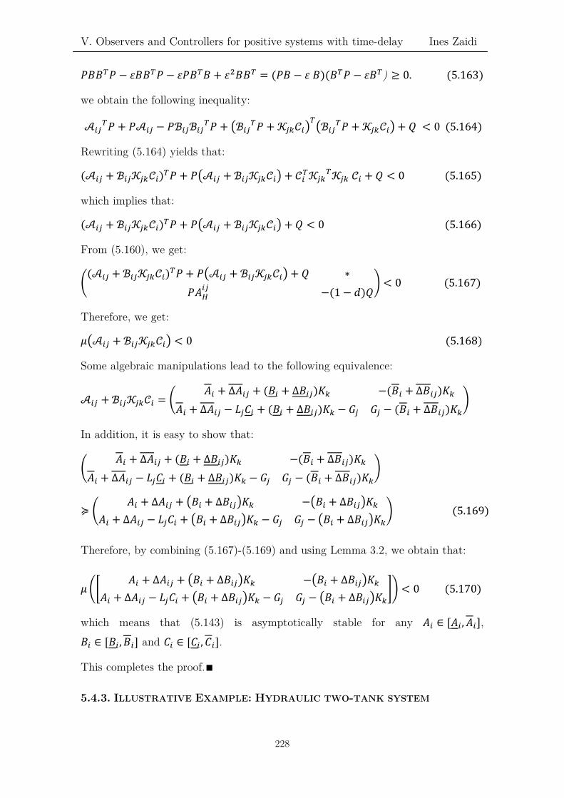
V. Observers and Controllers for positive systems with time-delay Ines Zaidi
𝑃𝑃𝐵𝐵𝐵𝐵𝑇𝑇𝑃𝑃 − 𝜀𝜀𝐵𝐵𝐵𝐵𝑇𝑇𝑃𝑃 − 𝜀𝜀𝑃𝑃𝐵𝐵𝑇𝑇𝐵𝐵 + 𝜀𝜀2𝐵𝐵𝐵𝐵𝑇𝑇 = (𝑃𝑃𝐵𝐵 − 𝜀𝜀 𝐵𝐵)(𝐵𝐵𝑇𝑇𝑃𝑃 − 𝜀𝜀𝐵𝐵𝑇𝑇) ≥ 0. (5.163)
we obtain the following inequality:
𝒜𝒜𝑚𝑚𝑖𝑖𝑇𝑇𝑃𝑃 + 𝑃𝑃𝒜𝒜𝑚𝑚𝑖𝑖 − 𝑃𝑃ℬ𝑚𝑚𝑖𝑖ℬ𝑚𝑚𝑖𝑖
𝑇𝑇𝑃𝑃 + �ℬ𝑚𝑚𝑖𝑖𝑇𝑇𝑃𝑃 + 𝒦𝒦𝑖𝑖𝑘𝑘𝒞𝒞𝑚𝑚�
𝑇𝑇�ℬ𝑚𝑚𝑖𝑖
𝑇𝑇𝑃𝑃 + 𝒦𝒦𝑖𝑖𝑘𝑘𝒞𝒞𝑚𝑚� + 𝑄𝑄 < 0 (5.164)
Rewriting (5.164) yields that:
(𝒜𝒜𝑚𝑚𝑖𝑖 + ℬ𝑚𝑚𝑖𝑖𝒦𝒦𝑖𝑖𝑘𝑘𝒞𝒞𝑚𝑚)𝑇𝑇𝑃𝑃 + 𝑃𝑃�𝒜𝒜𝑚𝑚𝑖𝑖 + ℬ𝑚𝑚𝑖𝑖𝒦𝒦𝑖𝑖𝑘𝑘𝒞𝒞𝑚𝑚� + 𝒞𝒞𝑚𝑚𝑇𝑇𝒦𝒦𝑖𝑖𝑘𝑘
𝑇𝑇𝒦𝒦𝑖𝑖𝑘𝑘 𝒞𝒞𝑚𝑚 + 𝑄𝑄 < 0 (5.165)
which implies that:
(𝒜𝒜𝑚𝑚𝑖𝑖 + ℬ𝑚𝑚𝑖𝑖𝒦𝒦𝑖𝑖𝑘𝑘𝒞𝒞𝑚𝑚)𝑇𝑇𝑃𝑃 + 𝑃𝑃�𝒜𝒜𝑚𝑚𝑖𝑖 + ℬ𝑚𝑚𝑖𝑖𝒦𝒦𝑖𝑖𝑘𝑘𝒞𝒞𝑚𝑚� + 𝑄𝑄 < 0 (5.166)
From (5.160), we get:
�(𝒜𝒜𝑚𝑚𝑖𝑖 + ℬ𝑚𝑚𝑖𝑖𝒦𝒦𝑖𝑖𝑘𝑘𝒞𝒞𝑚𝑚)𝑇𝑇𝑃𝑃 + 𝑃𝑃�𝒜𝒜𝑚𝑚𝑖𝑖 + ℬ𝑚𝑚𝑖𝑖𝒦𝒦𝑖𝑖𝑘𝑘𝒞𝒞𝑚𝑚� + 𝑄𝑄 ∗
𝑃𝑃𝐴𝐴𝐻𝐻𝑚𝑚𝑖𝑖 −(1 − 𝑑𝑑)𝑄𝑄
� < 0 (5.167)
Therefore, we get:
𝜇𝜇�𝒜𝒜𝑚𝑚𝑖𝑖 + ℬ𝑚𝑚𝑖𝑖𝒦𝒦𝑖𝑖𝑘𝑘𝒞𝒞𝑚𝑚� < 0 (5.168)
Some algebraic manipulations lead to the following equivalence:
𝒜𝒜𝑚𝑚𝑖𝑖 + ℬ𝑚𝑚𝑖𝑖𝒦𝒦𝑖𝑖𝑘𝑘𝒞𝒞𝑚𝑚 = �𝐴𝐴𝑚𝑚 + ∆𝐴𝐴𝑚𝑚𝑖𝑖 + (𝐵𝐵𝑚𝑚 + ∆𝐵𝐵𝑚𝑚𝑖𝑖)𝐾𝐾𝑘𝑘 −(𝐵𝐵𝑚𝑚 + ∆𝐵𝐵𝑚𝑚𝑖𝑖)𝐾𝐾𝑘𝑘
𝐴𝐴𝑚𝑚 + ∆𝐴𝐴𝑚𝑚𝑖𝑖 − 𝐿𝐿𝑖𝑖𝐶𝐶𝑚𝑚 + (𝐵𝐵𝑚𝑚 + ∆𝐵𝐵𝑚𝑚𝑖𝑖)𝐾𝐾𝑘𝑘 − 𝐺𝐺𝑖𝑖 𝐺𝐺𝑖𝑖 − (𝐵𝐵𝑚𝑚 + ∆𝐵𝐵𝑚𝑚𝑖𝑖)𝐾𝐾𝑘𝑘�
In addition, it is easy to show that:
�𝐴𝐴𝑚𝑚 + ∆𝐴𝐴𝑚𝑚𝑖𝑖 + (𝐵𝐵𝑚𝑚 + ∆𝐵𝐵𝑚𝑚𝑖𝑖)𝐾𝐾𝑘𝑘 −(𝐵𝐵𝑚𝑚 + ∆𝐵𝐵𝑚𝑚𝑖𝑖)𝐾𝐾𝑘𝑘
𝐴𝐴𝑚𝑚 + ∆𝐴𝐴𝑚𝑚𝑖𝑖 − 𝐿𝐿𝑖𝑖𝐶𝐶𝑚𝑚 + (𝐵𝐵𝑚𝑚 + ∆𝐵𝐵𝑚𝑚𝑖𝑖)𝐾𝐾𝑘𝑘 − 𝐺𝐺𝑖𝑖 𝐺𝐺𝑖𝑖 − (𝐵𝐵𝑚𝑚 + ∆𝐵𝐵𝑚𝑚𝑖𝑖)𝐾𝐾𝑘𝑘�
≽ �𝐴𝐴𝑚𝑚 + ∆𝐴𝐴𝑚𝑚𝑖𝑖 + �𝐵𝐵𝑚𝑚 + ∆𝐵𝐵𝑚𝑚𝑖𝑖�𝐾𝐾𝑘𝑘 −�𝐵𝐵𝑚𝑚 + ∆𝐵𝐵𝑚𝑚𝑖𝑖�𝐾𝐾𝑘𝑘
𝐴𝐴𝑚𝑚 + ∆𝐴𝐴𝑚𝑚𝑖𝑖 − 𝐿𝐿𝑖𝑖𝐶𝐶𝑚𝑚 + �𝐵𝐵𝑚𝑚 + ∆𝐵𝐵𝑚𝑚𝑖𝑖�𝐾𝐾𝑘𝑘 − 𝐺𝐺𝑖𝑖 𝐺𝐺𝑖𝑖 − �𝐵𝐵𝑚𝑚 + ∆𝐵𝐵𝑚𝑚𝑖𝑖�𝐾𝐾𝑘𝑘� (5.169)
Therefore, by combining (5.167)-(5.169) and using Lemma 3.2, we obtain that:
𝜇𝜇 ��𝐴𝐴𝑚𝑚 + ∆𝐴𝐴𝑚𝑚𝑖𝑖 + �𝐵𝐵𝑚𝑚 + ∆𝐵𝐵𝑚𝑚𝑖𝑖�𝐾𝐾𝑘𝑘 −�𝐵𝐵𝑚𝑚 + ∆𝐵𝐵𝑚𝑚𝑖𝑖�𝐾𝐾𝑘𝑘
𝐴𝐴𝑚𝑚 + ∆𝐴𝐴𝑚𝑚𝑖𝑖 − 𝐿𝐿𝑖𝑖𝐶𝐶𝑚𝑚 + �𝐵𝐵𝑚𝑚 + ∆𝐵𝐵𝑚𝑚𝑖𝑖�𝐾𝐾𝑘𝑘 − 𝐺𝐺𝑖𝑖 𝐺𝐺𝑖𝑖 − �𝐵𝐵𝑚𝑚 + ∆𝐵𝐵𝑚𝑚𝑖𝑖�𝐾𝐾𝑘𝑘�� < 0 (5.170)
which means that (5.143) is asymptotically stable for any 𝐴𝐴𝑚𝑚 ∈ [𝐴𝐴𝑚𝑚, 𝐴𝐴𝑚𝑚],
𝐵𝐵𝑚𝑚 ∈ [𝐵𝐵𝑚𝑚, 𝐵𝐵𝑚𝑚] and 𝐶𝐶𝑚𝑚 ∈ [𝐶𝐶𝑚𝑚 , 𝐶𝐶𝑚𝑚].
This completes the proof.∎
5.4.3. ILLUSTRATIVE EXAMPLE: HYDRAULIC TWO-TANK SYSTEM
228

V. Observers and Controllers for positive systems with time-delay Ines Zaidi
We consider, as an application, the process composed of two linked tanks stated in Section 3.3.2.4. (Benzaouia & Hajjaji, 2011), (Zhang & Ding, 2005).
Now, we synthesized an observer-based controller for the positive interval T-S model with unmeasurable premise variables (5.91), in order guarantee a good estimation for the state variables of the system.
We can write the time-delay model as follows:
��̇�𝑥(𝑡𝑡) = Ȃ(𝑧𝑧1, 𝑧𝑧2)𝑥𝑥(𝑡𝑡) + Ȃ𝜏𝜏(𝑧𝑧1, 𝑧𝑧2)𝑥𝑥�𝑡𝑡 − 𝜏𝜏(𝑡𝑡)� + 𝐵𝐵𝑢𝑢(𝑡𝑡) 𝑦𝑦(𝑡𝑡) = 𝐶𝐶 𝑥𝑥(𝑡𝑡) 𝑥𝑥(𝑡𝑡) = 𝜑𝜑(𝑡𝑡) ≽ 0, ∀ 𝑡𝑡 ∈ �−ℎ, 0�
(5.171)
where:
Ȃ =
⎝
⎜⎛
−𝑅𝑅1𝑧𝑧1 −𝑅𝑅12𝑧𝑧1𝑧𝑧2
�|𝑧𝑧12 − 𝑧𝑧2
2|0
0 −𝑅𝑅2𝑧𝑧2 −𝑅𝑅12𝑧𝑧1𝑧𝑧2
�|𝑧𝑧12 − 𝑧𝑧2
2|⎠
⎟⎞
(5.172)
and
Ȃ𝜏𝜏 =
⎝
⎜⎛
0𝑅𝑅12𝑧𝑧1𝑧𝑧2
�|𝑧𝑧12 − 𝑧𝑧2
2|𝑅𝑅12𝑧𝑧1𝑧𝑧2
�|𝑧𝑧12 − 𝑧𝑧2
2|0
⎠
⎟⎞
(5.173)
with 𝜏𝜏(𝑡𝑡) ∈ ℝ a time-varying delay, considered as a continuous function, satisfying
�0 ≤ 𝜏𝜏(𝑡𝑡) ≤ ℎ�̇�𝜏(𝑡𝑡) ≤ 𝑑𝑑 < 1
(5.174)
and expressed by:
𝜏𝜏(𝑡𝑡) =0.5
1 + 𝑡𝑡 , ∀ 𝑡𝑡 > 0 (5.175)
with 𝑅𝑅1, 𝑅𝑅2 and 𝑅𝑅12 positive physical constants, as shown in (Benzaouia & El Hajjaji, 2011).
So, ℎ = 0.5 and 𝑑𝑑 = 0.5.
We consider that the variables are bounded as follows:
𝑑𝑑1 ≤ 𝑧𝑧1 ≤ 𝑏𝑏1 (5.176)
229
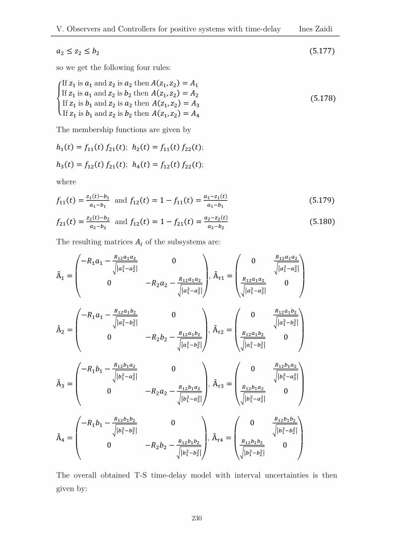
V. Observers and Controllers for positive systems with time-delay Ines Zaidi 𝑑𝑑2 ≤ 𝑧𝑧2 ≤ 𝑏𝑏2 (5.177)
so we get the following four rules:
⎩⎨
⎧If 𝑧𝑧1 is 𝑑𝑑1 and 𝑧𝑧2 is 𝑑𝑑2 then 𝐴𝐴(𝑧𝑧1, 𝑧𝑧2) = 𝐴𝐴1 If 𝑧𝑧1 is 𝑑𝑑1 and 𝑧𝑧2 is 𝑏𝑏2 then 𝐴𝐴(𝑧𝑧1, 𝑧𝑧2) = 𝐴𝐴2 If 𝑧𝑧1 is 𝑏𝑏1 and 𝑧𝑧2 is 𝑑𝑑2 then 𝐴𝐴(𝑧𝑧1, 𝑧𝑧2) = 𝐴𝐴3If 𝑧𝑧1 is 𝑏𝑏1 and 𝑧𝑧2 is 𝑏𝑏2 then 𝐴𝐴(𝑧𝑧1, 𝑧𝑧2) = 𝐴𝐴4
(5.178)
The membership functions are given by
ℎ1(𝑡𝑡) = 𝑓𝑓11(𝑡𝑡) 𝑓𝑓21(𝑡𝑡); ℎ2(𝑡𝑡) = 𝑓𝑓11(𝑡𝑡) 𝑓𝑓22(𝑡𝑡);
ℎ3(𝑡𝑡) = 𝑓𝑓12(𝑡𝑡) 𝑓𝑓21(𝑡𝑡); ℎ4(𝑡𝑡) = 𝑓𝑓12(𝑡𝑡) 𝑓𝑓22(𝑡𝑡);
where
𝑓𝑓11(𝑡𝑡) = 𝑗𝑗1(𝑡𝑡)−𝑏𝑏1𝑚𝑚1−𝑏𝑏1
and 𝑓𝑓12(𝑡𝑡) = 1 − 𝑓𝑓11(𝑡𝑡) = 𝑚𝑚1−𝑗𝑗1(𝑡𝑡)𝑚𝑚1−𝑏𝑏1
(5.179)
𝑓𝑓21(𝑡𝑡) = 𝑗𝑗2(𝑡𝑡)−𝑏𝑏2𝑚𝑚2−𝑏𝑏2
and 𝑓𝑓12(𝑡𝑡) = 1 − 𝑓𝑓21(𝑡𝑡) = 𝑚𝑚2−𝑗𝑗2(𝑡𝑡)𝑚𝑚2−𝑏𝑏2
(5.180)
The resulting matrices 𝐴𝐴𝑚𝑚 of the subsystems are:
Ȃ1 =
⎝
⎜⎛
−𝑅𝑅1𝑑𝑑1 − 𝑅𝑅12𝑚𝑚1𝑚𝑚2
��𝑚𝑚12−𝑚𝑚2
2�0
0 −𝑅𝑅2𝑑𝑑2 − 𝑅𝑅12𝑚𝑚1𝑚𝑚2
��𝑚𝑚12−𝑚𝑚2
2�⎠
⎟⎞
, Ȃ𝜏𝜏1 =
⎝
⎜⎛
0 𝑅𝑅12𝑚𝑚1𝑚𝑚2
��𝑚𝑚12−𝑚𝑚2
2�
𝑅𝑅12𝑚𝑚1𝑚𝑚2
��𝑚𝑚12−𝑚𝑚2
2�0
⎠
⎟⎞
Ȃ2 =
⎝
⎜⎛
−𝑅𝑅1𝑑𝑑1 − 𝑅𝑅12𝑚𝑚1𝑏𝑏2
��𝑚𝑚12−𝑏𝑏2
2�0
0 −𝑅𝑅2𝑏𝑏2 − 𝑅𝑅12𝑚𝑚1𝑏𝑏2
��𝑚𝑚12−𝑏𝑏2
2�⎠
⎟⎞
, Ȃ𝜏𝜏2 =
⎝
⎜⎛
0 𝑅𝑅12𝑚𝑚1𝑏𝑏2
��𝑚𝑚12−𝑏𝑏2
2�
𝑅𝑅12𝑚𝑚1𝑏𝑏2
��𝑚𝑚12−𝑏𝑏2
2�0
⎠
⎟⎞
Ȃ3 =
⎝
⎜⎛
−𝑅𝑅1𝑏𝑏1 − 𝑅𝑅12𝑏𝑏1𝑚𝑚2
��𝑏𝑏12−𝑚𝑚2
2�0
0 −𝑅𝑅2𝑑𝑑2 − 𝑅𝑅12𝑏𝑏1𝑚𝑚2
��𝑏𝑏12−𝑚𝑚2
2�⎠
⎟⎞
, Ȃ𝜏𝜏3 =
⎝
⎜⎛
0 𝑅𝑅12𝑏𝑏1𝑚𝑚2
��𝑏𝑏12−𝑚𝑚2
2�
𝑅𝑅12𝑏𝑏1𝑚𝑚2
��𝑏𝑏12−𝑚𝑚2
2�0
⎠
⎟⎞
Ȃ4 =
⎝
⎜⎛
−𝑅𝑅1𝑏𝑏1 − 𝑅𝑅12𝑏𝑏1𝑏𝑏2
��𝑏𝑏12−𝑏𝑏2
2�0
0 −𝑅𝑅2𝑏𝑏2 − 𝑅𝑅12𝑏𝑏1𝑏𝑏2
��𝑏𝑏12−𝑏𝑏2
2�⎠
⎟⎞
, Ȃ𝜏𝜏4 =
⎝
⎜⎛
0 𝑅𝑅12𝑏𝑏1𝑏𝑏2
��𝑏𝑏12−𝑏𝑏2
2�
𝑅𝑅12𝑏𝑏1𝑏𝑏2
��𝑏𝑏12−𝑏𝑏2
2�0
⎠
⎟⎞
The overall obtained T-S time-delay model with interval uncertainties is then given by:
230

V. Observers and Controllers for positive systems with time-delay Ines Zaidi
⎩⎪⎨
⎪⎧�̇�𝑥(𝑡𝑡) = � ℎ𝑚𝑚(𝑥𝑥(𝑡𝑡))(�Ȃ𝑚𝑚 + ∆Ȃ𝑚𝑚𝑖𝑖�𝑥𝑥(𝑡𝑡) + �Ȃ𝜏𝜏𝑚𝑚 + ∆Ȃ𝜏𝜏𝑚𝑚𝑖𝑖�𝑥𝑥�𝑡𝑡 − 𝜏𝜏(𝑡𝑡)� + 𝐵𝐵𝑢𝑢(𝑡𝑡))
4
𝑚𝑚=1
𝑦𝑦(𝑡𝑡) = 𝐶𝐶 𝑥𝑥(𝑡𝑡) 𝑥𝑥(𝑡𝑡) = 𝜑𝜑(𝑡𝑡) ≽ 0, ∀ 𝑡𝑡 ∈ [−𝜏𝜏, 0]
(5.181)
For calculation, we fix the parameters and their uncertainties as follows:
𝑅𝑅1 = 𝑅𝑅2 = 0.95 ± 0.02, 𝑅𝑅12 = 0.65 ± 0.03,
𝑑𝑑1 = 0.2236 ± 0.011, 𝑏𝑏1 = 0.4472 ± 0.021
𝑑𝑑2 = 0.2582 ± 0.016, 𝑏𝑏2 = 0.4082 ± 0.015
The objective is to design an interval observer-based controller which ensures the stabilization and the estimation of the system associated to the real plant, in which matrices Ȃ𝑚𝑚 + ∆Ȃ𝑚𝑚𝑖𝑖 are Metzler and matrices Ȃ𝜏𝜏𝑚𝑚 + ∆Ȃ𝜏𝜏𝑚𝑚𝑖𝑖, 𝐵𝐵 and 𝐶𝐶 are
nonnegative, ∀ 𝑖𝑖, 𝑗𝑗 = 1, … , 𝑟𝑟.
We have:
Ȃ1 = �−0.3878 00 −0.4163�; Ȃ1 = �−0.2541 0
0 −0.1653�
Ȃ2 = �−0.3935 00 −0.4067�; Ȃ2 = �−0.1250 0
0 −0.3908�
Ȃ3 = � −0.8881 00 −0.5128�; Ȃ3 = � −0.4623 0
0 −0.2752�
Ȃ4 = � −0.8669 00.2229 −0.4763�; Ȃ4 = � −0.5301 0
0 −0.3046�
Ȃ𝜏𝜏1 = � 0 0.01640.0164 0 �; Ȃ𝜏𝜏1 = � 0 0.0737
0.0292 0 �
Ȃ𝜏𝜏2 = � 0 0.01700.0170 0 �; Ȃ𝜏𝜏2 = � 0 0.0571
0.0258 0 �
Ȃ𝜏𝜏3 = � 0 0.02710.0271 0 �; Ȃ𝜏𝜏3 = � 0 0.0386
0.0443 0 �
Ȃ𝜏𝜏4 = � 0 0.02480.0248 0 �; Ȃ𝜏𝜏4 = � 0 0.0892
0.0732 0 �
𝐵𝐵 = �1 00 1� ; 𝐶𝐶 = (1 0)
where Ȃ𝑚𝑚, Ȃ𝑚𝑚, Ȃ𝜏𝜏𝑚𝑚 and Ȃ𝜏𝜏𝑚𝑚 correspond respectively to the state and delay matrices of the interval system (5.181), ∀ 𝑖𝑖 = 1, … ,4.
Applying Theorem 5.8. to the system (5.181), we get the following gain matrices:
231
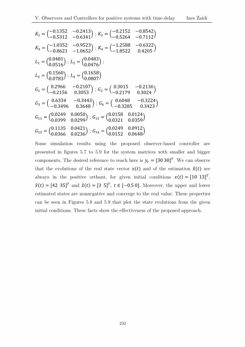
V. Observers and Controllers for positive systems with time-delay Ines Zaidi
𝐾𝐾1 = �−0.1352 −0.2413−0.5312 −0.6341� ; 𝐾𝐾2 = �−0.2152 −0.8542
−0.5264 −0.7112�
𝐾𝐾3 = �−1.0352 −0.9523−0.8621 −1.0652� ; 𝐾𝐾4 = �−1.2588 −0.6322
−1.8522 0.4205 �
𝐿𝐿1 = �0.04810.0516� ; 𝐿𝐿2 = �0.0483
0.0476� ;
𝐿𝐿3 = �0.15600.0783� ; 𝐿𝐿4 = �0.1658
0.0807�
𝐺𝐺1 = � 0.2966 −0.2107−0.2156 0.3053 � ; 𝐺𝐺2 = � 0.3015 −0.2136
−0.2179 0.3024 �
𝐺𝐺3 = � 0.6334 −0.3443 −0.3496 0.3648 � ; 𝐺𝐺4 = � 0.6048 −0.3224
−0.3285 0.3423 �
𝐺𝐺11 = �0.0249 0.00500.0399 0.0299� ; 𝐺𝐺12 = �0.0158 0.0124
0.0321 0.0359�
𝐺𝐺13 = �0.1135 0.04210.0366 0.0236� ; 𝐺𝐺14 = �0.0249 0.0912
0.0152 0.0648�
Some simulation results using the proposed observer-based controller are presented in figures 5.7 to 5.9 for the system matrices with smaller and bigger components. The desired reference to reach here is 𝑦𝑦𝑟𝑟 = [30 30]𝑇𝑇. We can observe that the evolutions of the real state vector 𝑥𝑥(𝑡𝑡) and of the estimation 𝑥𝑥�(𝑡𝑡) are always in the positive orthant, for given initial conditions 𝑥𝑥(𝑡𝑡) = [10 13]𝑇𝑇, 𝑥𝑥�(𝑡𝑡) = [42 35]𝑇𝑇 and 𝑥𝑥�(𝑡𝑡) = [3 5]𝑇𝑇, 𝑡𝑡 ∈ [−0.5 0]. Moreover, the upper and lower estimated states are nonnegative and converge to the real value. These properties can be seen in Figures 5.8 and 5.9 that plot the state evolutions from the given initial conditions. These facts show the effectiveness of the proposed approach.
232

V. Observers and Controllers for positive systems with time-delay Ines Zaidi
Figure 5. 7. Evolution of the two pump flows 𝑢𝑢1(𝑡𝑡) and 𝑢𝑢2(𝑡𝑡)
Figure 5. 8. Evolution of the state 𝑥𝑥1(𝑡𝑡) and its estimation 𝑥𝑥�1(𝑡𝑡)
233

V. Observers and Controllers for positive systems with time-delay Ines Zaidi
Figure 5. 9. Evolution of the state 𝑥𝑥2(𝑡𝑡) and its estimation 𝑥𝑥�2(𝑡𝑡)
5.5. Conclusion
In this section, we have dealt with the problem of observer-based control design for positive time-delay systems. Firstly, we have designed positive observers for positive interval linear time-delay systems; necessary and sufficient conditions have been established, taking into account the positivity constraints. Secondly, observer-based controllers have been synthesized for this class of systems. Necessary conditions have been established in order to verify the existence of an observer-based controller for the considered closed-loop system. Once satisfied, we study the sufficient conditions and the corresponding synthesis for this problem. Then, we extend these approaches for positive interval time-delay T-S systems. For this, we consider two cases: when the decision variables are measurable and when the decision variables are unmeasurable.
Finally, illustrative results of numerical and practical examples have been given to show the effectiveness of these approaches.
234

V. Observers and Controllers for positive systems with time-delay Ines Zaidi
235

Conclusions and Perspectives Ines Zaidi
236

Conclusions and Perspectives Ines Zaidi
Conclusions and Perspectives
237

Conclusions and Perspectives Ines Zaidi
238

Conclusions and Perspectives Ines Zaidi
6.1. Summary and Contributions
This thesis firstly presents systematic procedures to design robust controllers and observer-based controllers for positive linear and T-S systems, with/without time-delay and with/without interval uncertainties. These approaches are based on the resolution of optimization problems, expressed as LMIs (Linear Matrix Inequalities). Furthermore, the proposed methodologies are extended to constrained design problems. These techniques have been applied on numerical and practical examples from literature, giving satisfactory results.
More precisely, the main contributions of the first part of this work lead to establish approaches to stabilize and to solve the problem of designing decomposed state-feedback controllers for positive linear and T-S systems, which can be subject to interval uncertainties. We have also presented the robust 𝛼𝛼-stability notion that guarantees a specified decay rate in the presence of possible uncertainties on the considered types of systems. Moreover, necessary and sufficient conditions are given for the stabilization of positive T-S systems, taking into account two cases: when the decision variables of the system are measurable or not. This may be provided by means of state-feedback laws that can be chosen with or without memory. Our contribution is mainly focused in the field of robust estimation through designing positive observer-based controllers and positive interval observer-based controllers for these types of systems, which can have interval uncertainties.
In this thesis, the theoretical developments improving interval estimations have been given and their efficiency has been demonstrated through various examples with significant uncertainties. It has been shown that the existence of robust interval positive observer-based controllers can be expressed in terms of LMI conditions, so they can be easily computed. The second part of this dissertation is devoted to the stability analysis, stabilization and observer-based control design of positive time-delay positive linear and T-S systems.
We consider in this thesis different types of delays: constant, variable, single and multiple. Techniques of stabilization and observer-based control of these systems have been established, corresponding to the considered time-delay and expressed in terms of LMI conditions.
239

Conclusions and Perspectives Ines Zaidi
Illustrative examples have shown the performance of the proposed approaches and we have proposed some practical applications: electrical systems and hydraulic systems.
6.2. Future Lines of Research
The work presented in this dissertation is an open research line and inspires to several interesting problems in the fields of control and estimation. Other interesting issues will be investigated such as static and dynamic output-feedback controller design for positive T-S systems with and without delay. Moreover, we tend for applying the approaches of this thesis on photovoltaic systems.
In addition, there exist more extensions under study. Among them, we can cite:
• Positive descriptor design for positive T-S systems with time-varying delays.
• Diagnosis and faults detection for positive T-S systems with time-varying delay.
• Positive multi-dimensional systems. • Positive LPV systems. • Implementation of the results to more practical systems.
Mostly, in the area of faults detection and isolation, interval observers and interval observer-based controllers using decomposed control laws can have a great importance. This can open the doors for multiple lines of future research.
Also, interval observation can provide useful estimates for robust control, where the control strategy and the interval estimates complement each other in order to deal with the uncertainties of the system and to guarantee a better level of performance.
240

Annex Ines Zaidi
Annex: Important Lemmas
B.1. Schur Complement
Let us consider three matrices 𝑄𝑄(𝑥𝑥), 𝑆𝑆(𝑥𝑥) and 𝑅𝑅(𝑥𝑥), affine with respect to the variable 𝑥𝑥. Matrices 𝑄𝑄(𝑥𝑥) and 𝑅𝑅(𝑥𝑥) are symmetric. The LMI:
�𝑄𝑄(𝑥𝑥) 𝑆𝑆(𝑥𝑥)𝑆𝑆(𝑥𝑥)𝑇𝑇 𝑅𝑅(𝑥𝑥)� > 0 ⇔ �
𝑅𝑅(𝑥𝑥) > 0 𝑄𝑄(𝑥𝑥) − 𝑆𝑆(𝑥𝑥)𝑅𝑅(𝑥𝑥)−1𝑆𝑆(𝑥𝑥)𝑇𝑇 > 0 (𝐵𝐵. 1.1)
B.2. (Zhou & Khargonedkar, 1988)
Consider two matrices 𝑋𝑋 and 𝑌𝑌 of appropriate dimensions. The following inequality is always applicable for every matrix 𝑄𝑄 = 𝑄𝑄𝑇𝑇 > 0:
𝑋𝑋𝑌𝑌𝑇𝑇 + 𝑌𝑌𝑋𝑋𝑇𝑇 ≤ 𝑋𝑋𝑄𝑄𝑋𝑋𝑇𝑇 + 𝑌𝑌𝑄𝑄−1𝑌𝑌𝑇𝑇 (𝐵𝐵. 1.2)
B.3. (Kacem, 2009)
Consider 𝜙𝜙, 𝑑𝑑, 𝑏𝑏 matrices with appropriate dimensions. The following hypotheses are equivalent:
a-The LMI
� 𝜙𝜙 𝑑𝑑𝑑𝑑𝑇𝑇 0
� + 𝑆𝑆𝑦𝑦𝐼𝐼 ��𝐹𝐹1𝐹𝐹2
� (𝑏𝑏𝑇𝑇 − 𝐼𝐼)� < 0 (𝐵𝐵. 1.3)
is feasible for the variables 𝐹𝐹1 and 𝐹𝐹2.
b-Matrices 𝜙𝜙, 𝑑𝑑 and 𝑏𝑏 verify the condition: 𝜙𝜙 + 𝑑𝑑𝑏𝑏𝑇𝑇 + 𝑏𝑏𝑑𝑑𝑇𝑇 < 0.
B.4. (Kacem, 2009)
Consider 𝜙𝜙, 𝑑𝑑, 𝑏𝑏 matrices with appropriate dimensions. The following hypotheses are equivalent:
a- 𝜙𝜙, 𝑑𝑑 and 𝑏𝑏 verify:
�𝜙𝜙 < 0 𝜙𝜙 + 𝑑𝑑𝑏𝑏𝑇𝑇 + 𝑏𝑏𝑑𝑑𝑇𝑇 < 0 (𝐵𝐵. 1.4)
b-The following LMI:
� 𝜙𝜙 𝑑𝑑 + 𝑏𝑏𝐺𝐺𝑇𝑇
𝑑𝑑𝑇𝑇 + 𝐺𝐺𝑏𝑏𝑇𝑇 −𝐺𝐺 − 𝐺𝐺𝑇𝑇� = � 𝜙𝜙 𝑑𝑑𝑑𝑑𝑇𝑇 0
� + 𝑆𝑆𝑦𝑦𝐼𝐼 ��0𝐼𝐼 � 𝐺𝐺(𝑏𝑏𝑇𝑇 − 𝐼𝐼)� < 0 (𝐵𝐵. 1.5)
is feasible for the variable 𝐺𝐺.
241

Annex Ines Zaidi
242

Bibliography Ines Zaidi
Bibliography A
Akar, M., & Ozuner, U. (1998). Stability and stabilization of T-S fuzzy systems. In Proceedings of the American Control Conference (ACC), 3840-3845, Philadelphia, USA.
Akar, M., & Ozuner, U. (2000). Decentralized techniques for the analysis and control of T-S fuzzy systems. IEEE Transactions on Fuzzy Systems, 8(6), 691-704.
Alamo, T., Bravo, J., & Camacho, E. (2005). Guaranteed state estimation by zonotypes. Automatica, 41(6), 1035-1043.
Akhenak, A. (2004). Conception d’observateurs non linéaires par approche multi-modèle : application au diagnostic. Thèse de doctorat, Institut National Polytechnique de Lorraine, Nancy, France.
Ariba, Y. (2009). Sur la stabilité des systèmes à retards variant dans le temps: théorie et application au contrôle de congestion d’un routeur. Thèse de doctorat, Université Toulouse 3 Paul Sabatier (UT3 Paul Sabatier).
B
Bara, G. I. (2001). Estimation d’état des systems à paramètres variants. Doctorat de l’institut National Polytechnique de Lorraine, Nancy.
Bapat, R. B., & Raghavan, T. E. S. (1997). Nonnegative matrices and applications. Cambridge University Press.
Benhadj Braiek, N. & Rotella, F. (1995). State observer design for a class of nonlinear system. Journal of Systems Analysis, Modelling and Simulation, 17, 265-277.
Benton, R. E., & Smith, D. (1997). Output feedback stabilization with prescribed degree of stability. In Proceedings of the American Control Conference (ACC), Albuquerque, New Mexico, 499-504.
243

Bibliography Ines Zaidi
Benvenuti, L., & Farina, L. (2002). Positive and compartmental systems. IEEE Transactions on Automatic Control, 47(2), 370–373.
Benzaouia, A., Hmamed, A., & El Hajjaji, A. (2001). Stabilization of positive discrete-time fuzzy systems by state feedback control. International Journal of Adaptive Control and Signal Processing.
Benzaouia, A., El Hajjaji, A., & Naib, M. (2006). Stabilization of a class of constrained fuzzy systems: A positive invariance approach. International Journal of Innovative Computing, Information and Control, 2(4), 749-760.
Benzaouia, A., Mehdi, D., El Hajjaji, A., & Nachidi, M. (2007). Piecewise quadratic lyapunov function for nonlinear systems with fuzzy static output feedback control. European Control Conference, Kos, Greece.
Benzaouia, A., & Tadeo, F. (2008), Stabilization of positive discrete-time switching systems by output feed-back. In Proceedings of the 16th Med.
Conference on Control and Automation, Ajaccio, France.
Benzaouia, A., & Tadeo, F. (2010). Stabilization of positive switching linear discrete-time systems. International Journal of Innovative Computing, Information and Control, 6(6), 2427-2437.
Benzaouia, A., Hmamed, A., & El Hajjaji, A. (2010). Stabilization of controlled positive discrete-time T-S fuzzy systems by state-feedback control. In International Journal of Adaptive Control and Signal Processing, 24(12), 1091-1106.
Benzaouia, A., Oubah, R., El Hajjaji, A., & Tadeo, F. (2011). Stability and stabilization of positive Takagi-Sugeno fuzzy continuous systems with delay. In Proceedings of the 50th IEEE Conference on Decision and Control and European Control Conference (CDC-ECC).
Benzaouia, A., El Hajjaji, A., & Tadeo, F. (2011a). Stabilization of switching T-S systems by switched Lyapunov function. International Journal of Adaptive Control and Signal Processing, 25(12), 1039-1049.
Benzaouia, A., & El Hajjaji, A. (2011). Delay-dependent stabilization conditions of controlled positive T-S fuzzy systems with time-varying delay. International
Journal of Innovative Computing, Information and Control, 7(4), 1533-1547.
244

Bibliography Ines Zaidi
Benzaouia, A., & Oubah, R. (2014). Stability and stabilization by output-feedback control of positive T-S fuzzy discrete-time systems with multiple delays. Nonlinear analysis: Hybrid systems, 11, 154-170.
Benzaouia, A., & El Hajjaji, A. (2014). Stabilization of discrete-time T-S fuzzy positive systems with multiple delays. Advanced Takagi-Sugeno Fuzzy Systems,
Studies in Decision and Control, 8, 209-249.
Benzaouia, A., Oubah, R., & El Hajjaji, A. (2014). Stabilization of positive T-S fuzzy discrete-time systems with multiple delays and bounded controls. Journal of
the Franklin Institute, 351(7), 3719-3733.
Bergsten, P., & Palm, R. (2000). Thau-Luenberger observers for T-S fuzzy systems. In Proceedings of the 9th IEEE International Conference on Fuzzy Systems, FUZZ IEEE, San Antonio, Texas, USA.
Bergsten, P., Palm, R., & Driankov, D. (2001). Fuzzy observers. In Proceedings of IEEE International Fuzzy Systems Conference, Melbourne, Australia.
Bergsten, P., Palm, R., & Driankov, D. (2002). Observers for Takagi-Sugeno fuzzy systems. IEEE Transactions on Systems, Man, and Cybernetics - Part B: Cybernetics, 32(1), 114–121.
Berman, A., Neumann, M., & Stern, R J. (1989). Nonnegative Matrices in Dynamic Systems. Wiley, New York.
Berman, A., & Plemmons, R. J. (1994). Nonnegative Matrices in The Mathematical Sciences. PA: SIAM, Philadelphia.
Bernussou, J. (1996). Commande robuste. Hermes ed. Paris, France.
Blanco, Y., Perruquetti, W., Borne, P. (2001). Stability and stabilizability of nonlinear systems and T-S fuzzy models. In Mathematical Problems in Engineering, (7), 221-240.
Bolajraf, M., Tadeo, F., Alvarez, T., & Rami, M. A. (2009). Control of routers in computer networks: a positive systems approach. In Proceedings of the 10th International Conference on Sciences and Techniques of Automatic Control and Computer Engineering, Hammamet, Tunisia.
245

Bibliography Ines Zaidi
Bolajraf, M., Tadeo, F., Alvarez, T., & Rami, M. A. (2010). State-feedback with memory for controlled positivity with application to congestion control. IET Control Theory and Applications, 4(10), 2041-2048.
Bolajraf, M., Rami, M. A., & Helmke, U. (2011). Robust positive interval observers for uncertain positive systems. In IFAC World Congress, 14330-14334, Milano, Italy.
Bolajraf, M. (2012). Robust control and estimation of positive systems. PhD dissertation, University of Valladolid, Spain.
Borne, P., Dauphin, T. G., Richard, J. P., Rotella, F., & Zambettakis, I. (1990). Commande et Optimisation des Processus. Technip, Collection Méthodes et Pratiques de l’Ingénieur ed, France.
Borne, P., Richard, J. P., & Radhy, N. E. (1993). Stability, stabilization, regulation: approche par les normes vectorielles. Masson edition, 2, de Systèmes non linéaires: Stabilité-Stabilisation, Paris, France.
Boukas, E., & El Hajjaji, A. (2006). On stabilizability of stochastic fuzzy systems. Proc. of the 2006 American Control Conference, 4362-4366, Minneapolis, MN.
Boukas, E. K. (2008). Free weighting matrices delay-dependent stabilization for systems with time-varying delays. ICIC Express Letters, 2(2), 167-173.
Boyd, S., El Ghawi, L., Feron, E., & Balakrishnan, V. (1994). Linear matrix inequalities in systems and control theory. Philadelphia, PA:SIAM.
Buslowicz, M. (2004). Robust stability of positive disrete-time linear systems with multiple delays with linear unit rank uncertainty structure or non-negative perturbation matrices. Bulletin of the Polish Academy of Sciences: Technical Sciences, (52), 99-102.
C
Cao, S. G., Rees, N. W., & Feng, G. (1999). Analysis and design of fuzzy control systems using dynamic fuzzy state space models. IEEE Transactions on Fuzzy Systems, 7(2), 192-200.
246

Bibliography Ines Zaidi
Cao, Y. Y., & Franck, P. M. (2000). Analysis and synthesis of nonlinear time-delay system via fuzzy control approach. IEEE Transactions on Fuzzy Systems, 8(2), 200- 211.
Cao, Y. Y, & Frank, P. M. (2001). Stability analysis and synthesis of nonlinear time-delay systems via linear Takagi-Sugeno fuzzy models. Fuzzy Sets and Systems, 124, 213-229.
Caswell, H. (2001). Matrix Population Models: Construction, Analysis and Interpretation. Sunderland, MA: Sinauer Association.
Chadli, M., Maquin., D., & Ragot., J. (2000). Relaxed stability conditions for Takagi-Sugeno fuzzy systems. In Proceedings of the IEEE International Conference on Systems, Man and cybernetics, 3514-3519, Nashville, USA.
Chadli, M., Maquin, D., & Ragot, J. (2001). On the stability analysis of multiple model. In Proceedings of the ECC, 1894-1899, Porto, Portugal.
Chadli, M., Maquin, D., & Ragot, J. (2002a). An LMI formulation for output-feedback stabilisation in multiple model approach. In Proceedings of the IEEE 41st CDC, Las Vegas, Nevada.
Chadli, M., Maquin, D., & Ragot, J. (2002b). Static output feedback for Takagi-Sugeno systesm: an LMI approach. In Proceedings of the 10th Mediterranean Conference on Control and Automation MED'02, Lisbon, Portugal.
Chadli, M., Maquin, D. & Ragot, J. (2002c). Observer based controller on the Takagi-Sugeno models. In Proceedings of IEEE International Conferences on System, Man and Cybernetics, 5, Tunisia.
Chadli, M., Maquin, D., & Ragot, J. (2002d). Sur la stabilité des modèles de Takagi-Sugeno: Approche quadratique. Journal Européen des systèmes automatisés (JESA), Soumis.
Chadli, M. (2002). Stabilité et commande des systèmes décrits par des multimodèles. Thèse de doctorat, Institut National Polytechnique, Lorraine, France.
247

Bibliography Ines Zaidi
Chadli, M., Maquin, D., & Ragot, J. (2004). Stabilization of Takagi-Sugeno models with maximum convergence rate. In Proceedings of the IEEE International Conference on Fuzzy Systems, 3, 1323-1326, Hungary.
Chen, G., Wang, J., & Shieh, L. S. (1997). Interval Kalman filtering. IEEE Transactions on Aerospace and Electronic Systems, 33(1), 250-259.
Chen, J., & Patton, R. (1999). Robust model-based fault diagnosis for dynamic systems. Kluwer Academic publisher.
Chen, B., & Liu, X. (2005a). Fuzzy guaranteed cost control for nonlinear systems with time-varying delay, IEEE Transactions on Fuzzy Systems, 13(2), 238-249.
Chen, B., & Liu, X. (2005b). Delay-dependent robust control for T-S fuzzy systems with time delay. IEEE Transactions on fuzzy systems, 13(4), 544-556.
Chen, W., & Saif, M. (2007). Design of a T-S based fuzzy nonlinear unknown input observer with fault diagnosis applications. In American Control Conference, New York City, USA.
Chen, B., Liu, X., & Liu, K. (2009). Robust 𝐻𝐻1 control of T-S fuzzy system with state and input time delays, Fuzzy Sets and Systems, 160, 403-422.
Cheng, C. M., Rees, N. W., & Feng, G. (1996). Stability analysis of fuzzy continuous-time dynamic systems. In Proceedings of the ICARCV, 1269-1273, Singapore.
Chilali, M., & Gahinet, P. (1996). 𝐻𝐻∞ Design with pole placement constraints: An LMI approach. IEEE Transactions on Automatic Control, 41(3), 358-367.
D
D’Alessandro, P., & de Santis, E. (1994). Positiveness of dynamic systems with non positive coefficient matrices. IEEE Transactions on Automatic Control. 39(1), 131-134.
Darouach, M., Zasadzinski, M., & Xu, S. (1994). Full-order observers for linear systems with unknown inputs. IEEE Transactions on Automatic Control, 39(3), 606–609.
248
Bibliography Ines Zaidi
De Leenheer, P., & Aeyels, D. (2001). Stabilization of positive linear systems. Systems and Control Letters, 44(4), 259-271.
Dilanech, I. (2009). Etude de la commande et de l’observation à distance de système. Thèse de doctorat, Université de Cergy-Pontoise, Paris, France.
Ding, S. X. (2008). Model-Based Fault Diagnosis Techniques Design Schemes, Algorithms, and Tools. Springer-Verlag.
E
El Ghaoui, L., & Rami, M. A. (1996). Robust stabilization of jump linear systems using linear matrix inequalities. International Journal of Robust and Nonlinear Control, 6(9-10), 1015-1023.
El Hajjaji, A., Benzaouia, A., & Naib, M. (2006). Stabilization of fuzzy systems with constrained controls by using positively invariant sets. Mathematical Problems for Engineering, 1-17.
El Hajjaji, A., & Chadli, M. (2008). Commande basée sur la modélisation floue de type Takagi-Sugeno d'un procédé expérimental à quatres cuves. CIFA Conference, Bucarest.
F
Farina, L., & Rinaldi, S. (2000). Positive Linear Systems: Theory and Applications, Wiley, New York.
Farza, M. (2000). Modélisation et synthèse d'observateurs pour les classes des systèmes non linéaires: application aux procédés (bio)chimiques. Habilitation, INPG, Grenoble.
Feng, G. (2002). Stability analysis of piecewise discrete-time linear systems. IEEE Transactions on Automatic Control, 7(7), 1108-1111.
Fridman, E., & Shaked, U. (2000). Stability and guaranteed cost control of uncertain discrete delay systems. International Journal of Control, 45(12), 2406–
2411.
249

Bibliography Ines Zaidi
Fridman, E., & Shaked, U. (2002). A descriptor system approach to 𝐻𝐻∞ control of linear time-delay systems. IEEE Transactions on Automatic Control, 47(2), 253–
270.
Fornasini, E., & Valcher, M. E. (2010). Linear Copositive Lyapunov Functions for Continuous-Time Positive Switched Systems. IEEE Transactions on Automatic Control. 55(8), 1933 -1937.
Frobenius, G. (1908). Uber matrizen aus positive elementen. Sitzungsberichte Konigl. Preussichen Akad. Wiss, 8, 471-476.
G
Gahinet, P., Becker, G., & Apkarian P. (1995). Self-scheduled 𝐻𝐻∞ control of linear parameter varying systems: a design example. Automatica, 31, 1251-1261.
Gahinet, P., Apkarian, P., & Chilali, M. (1996). Affine parameter-dependent Lyapunov functions and real parametric uncertainty. IEEE Transactions on Automatic Control, 41(3), 436-442.
Gao, H. J., & Wang, C. H. (2003). Comments and further results on a descriptor system approach to 𝐻𝐻∞ control of linear time-delay systems. IEEE Transactions
on Automatic Control, 48(3), 520–525.
Gao, H., Lam, J., & Wang, Ch. (2005). Control for Stability and Positivity: Equivalent Conditions and Computation. In IEEE Transactions on Circuits and Systems. 52(9).
Garcia, G. (1997). Contribution à la synthèse de lois de commande robuse par l’approche quadratique. HDR, Université Paul Sabatier, Rapport LASS no. 97543.
Garcia, G., Pradin, B., & Zeng, F. Y. (2001). Stabilization of discrete-time linear systems by static output feedback. IEEE Transactions on Automatic Control. 46(12), 1954-1957.
Gassara, H., El Hajjaji, A., & Chaabane, M. (2009a). Robust stability and stabilization conditions for time-delay fuzzy systems using fuzzy weighting-dependent approach. In Proceedings of European Control Conference, 23-26, Budapest, Hungary.
250
Bibliography Ines Zaidi
Gassara, H., El Hajjaji, A., & Chaabane, M. (2009b). Delay-dependent stabilization conditions of T-S fuzzy systems with time varying delay. In Proceedings of the 17th Mediterranean Conference on Control and Automation, Thessaloniki, Greece.
Gassara, H., El Hajjaji, A., & Chaabane, M. (2009c). Robust Control of T-S fuzzy systems with Time-varying delay: New approach. In Proceedings of the 48th IEEE Conference on Decision and Control, Shanghai, P.R. China.
Gassara, H., El Hajjaji, A., & Chaabane, M. (2010b). Robust Control of T-S fuzzy systems with Time-varying delay using new approach. International Journal of Robust and Nonlinear Control, 20(14), 1566-1578.
Gassara, H., El Hajjaji, A., & Chaabane, M. (2010c). Robust 𝐻𝐻1 Control for T-S fuzzy systems with time varying delay, International Journal of Systems Science, 41(12), 1481-1491.
Gasso, G. (2000). Identification de systèmes dynamiques non linéaires: approche multi-modèle. Thèse de doctorat, Institut National Polytechnique de Lorraine (INPL), Nancy, France.
Gauthier, J., Hammouri, H., & Othman, S. (1992). A simple observer for nonlinear systems applications to bioreactors. IEEE Transactions on Automatic Control, 37(6), 875–880.
Geromel, J. C., Peres, P. L., & Souza, S. R. (1996). Convex analysis of output feedback control problems: robust stability and performance. IEEE Transactions on Automatic Control. 41(7), 997-1003.
Gertler, J. (1998). Fault detection and diagnosis in engineering systems. Marcel Dekker.
Golub, G. H. & Loan, C. F. V. (1996). Matrix Computations. MD: Johns Hopkins University Press, Baltimore.
Gong, C., & Su, B. (2009). Delay-dependent robust stabilization for uncertain stochastic fuzzy system with time-varying delays. International Journal of
Innovative Computing, Information and Control, 5(5), 1429-1440.
251

Bibliography Ines Zaidi
Gopalsamy. K. (1992). Stability and Oscillations in Delay Differential Equations of Population Dynamics. Kluwer Academic Publishers.
Gouzé, J. L., Rapaport, A., & Haji-Sadok, M. (2000). Interval observers for uncertain biological systems. Ecological Modelling, 133(1-2), 45-56.
Gu, K. (1997). Discretized LMI set in the stability problem of linear uncertain time delay systems. International Journal of Control, 68, 923–934.
Gu, K. (1999). Discretized Lyapunov functional for uncertain systems with multiple time-delay. International Journal of Control, 72, 1436–1445.
Gu, K., & Han, Q. L. (2000). Discretized Lyapunov functional for linear uncertain systems with time-varying delay. In Proceedings of the American Control
Conference, 1375–1379.
Guan, X. P., & Chen, C. L. (2004). Delay-dependent guaranteed cost control for T-S fuzzy systems with time delays. IEEE Transactions on Fuzzy Systems, 12(2),
236-249.
Guerra, T. M., Vermeiren, L., Delmotte, F., & Borne, P. (1999). Lois de commande pour systèmes flous continus. APII-JESA, Hèrmes Science, 33(4), 489–527.
Guerra, T. M., & Vermeiren, L. (2001). Control laws for Takagi-Sugeno fuzzy models. Fuzzy Sets and Systems, 33(120), 95-108.
Guerra, T. M., Kruszewski, A., Vermeiren, L. & Tirmant, H. (2006). Conditions of output stabilization for nonlinear models in the Takagi-Sugeno’s form. Fuzzy Sets Systems. 157, 1248-1259.
H
Haddad, W. M., & Chellaboina, V. (2004). Stability theory for nonnegative and compartmental dynamical systems with time delay. Systems and Control letters, 2, 1422-1427.
Haddad, W. M., & Chellaboina, V. S. (2005). Stability and dissipativity theory for nonnegative dynamical systems: A unified analysis framework for biological
252

Bibliography Ines Zaidi
and physiological systems. Nonlinear Analysis: Real World Applications, 6(1), 35–65.
Haddad, W. M., Chellaboina, V., & Hui, Q. (2010). Nonnegative and Compartmental Dynamical Systems. Princeton University Press.
Hale, J. (1977). Theory of functional differential equations. Springer-Verlag.
Han, Q. L., & Mehdi, D. (1999). Robust 𝐻𝐻∞ controller synthesis for uncertain systems with multiple time-varying delays: An LMI approach. In Proceedings of
the 14th IFAC World Congress, Beijing, P. R. China.
Han, Z. X., Feng, G., Walcort, B. L., & Ma, J. (2000). Dynamic output-feedback controller design for fuzzy systems. IEEE Transactions on Systems Man and Cybernetics-part C, 30(1), 204-210.
Han, Q. L., & Gu, K. (2001). Stability of linear systems with time-varying delay: A generalized discretized Lyapunov functional approach. Asian Journal of
Control, 3, 170–180.
Han, Q. L. (2002). New results for delay-dependent stability of linear systems with time-varying delay. International Journal of Systems Science, 33, 213–228.
Han, Q. L. (2005). Absolute stability of time-delay systems with sector-bounded nonlinearity. Automatica, 41, 2171–2176.
Han, H. (2009). Delay-dependent fuzzy control designs for a class of nonlinear systems, International Journal of Innovative Computing, Information and
Control, 5(12B), 5041-5050.
Han, H., & Liu, Liu, Y. (2009). Further results on T-S fuzzy model with time delay. ICIC Express Letters, 3(4B), 1405-1410.
Hassibi, A., & Boyd, S. (1998). Quadratic stabilization and control of piecewise linear systems. In Proceedings of the CDC, 3659-3664, Florida, USA.
He, Y., Wang, Q. G., Lin, C., & Wu, M. (2007). Delay-range-dependent stability for systems with time-varying delay. Automatica, 43, 371–376.
253

Bibliography Ines Zaidi
Heemels, W. P. M. H, Van Eijndhoven, S. J. L, & Stoorvogel, A. A. (1998). Linear quadratic regulator problem with positive controls. International Journal of Control, 70, pp. 551–578.
Hof, V. D. J. M. (1997). Realization of continuous-time positive linear systems. Systems and Control Letters, 31(4), 243-253.
Hof, J. M. V. D. (1998). Positive linear observers for linear compartmental systems. SIAM Journal of Control and Optimization, 36(2), 590-608.
Hofbauer, J., & Sigmund, K. (1998). Evolutionary Games and Population Dynamics. Cambridge University Press, Cambridge, UK.
Hmamed, A., Benzaouia, A., Rami, M. A., & Tadeo. F. (2007). Positive stabilization of discrete-time systems with unknown delay and bounded controls. In Proceedings of the European Control Conference, Kos, Greece.
Hmamed, A., Benzaouia, A., Rami, M. A., & Tadeo, F. (2008). Memoryless control to Drive States of Delayed Continuous-time Systems within the Nonnegative Orthant. In Proceedings of the 18th World Congress IFAC, Seoul, Korea, July 6-11.
I
Ichalal, D., Marx, B., Ragot, J., & Maquin, D. (2007). Conception de multi-observateurs à variables de décisions non mesurables. In Journées Doctorales en Modélisation, Analyse et Conduite des Systèmes dynamiques (JDMACS), Reims, France.
Ichalal, D., Marx, B., Ragot, J. & Maquin D. (2008a). Design of observers for Takagi-Sugeno systems with immeasurable premise variables: an 𝐿𝐿2 approach. In Proceedings of the 17th IFAC World Congress, Seoul, South Korea.
Ichalal, D., Marx, B., Ragot, J. & Maquin, D. (2008b). Multi-Observateurs à entrées inconnues pour système de Takagi-Sugeno à variables de décision non mesurables. In Cinquième Conférence Internationale Francophone d’Automatique (CIFA), Bucarest, Romania.
254

Bibliography Ines Zaidi
Ichalal D., Marx B., Ragot J., & Maquin, D. (2008c). Diagnostic des systèmes non linéaires par approche multimodèle. In Workshop Surveillance, Sûreté et Sécurité des Grands Systèmes (3SGS'08), Troyes, France.
Ichalal, D. (2009). Estimation et diagnostic de systèmes non linéaires décrits par un modèle de Takagi-Sugeno. PhD thesis, Université de Nancy, France.
Isermann, R. (2007). Fault-diagnosis systems: An introduction from fault detection to fault tolerance. Springer.
Isidori, A. (1999). Nonlinear Control Systems II. Springer Verlag. London.
J
Jacquez, J. A., Simon, C. P. (1993). Qualitative theory of compartmental systems. SIAM Review, 43–79.
Jadbabaie, A. (1999). A reduction in conservatism in stability and 𝐿𝐿2 gain analysis of Takagi-Sugeno fuzzy systems via linear matrix inequalities. In Proceedings of the IFAC, 285-289, China.
Jaulin, L., Kieffer, M., Didrit, O., & Walter, E. (2001). Applied interval analysis, with examples in parameter and state estimation, robust control and robotics. Springer London Ltd, United Kingdom.
Jaulin, L. (2002). Nonlinear bounded error state estimation of continuous time systems. Automatica, 38(6), 1079-1082.
Jeung, E., Oh, D., Kim, J., & Park, H. B. (1996). Robust controller design for uncertain systems with time delays: LMI approach. Automatica, 32, 1229–1231.
Jiang, X., & Han, Q. L. (2006). Delay-dependent robust stability for uncertain linear systems with interval time-varying delay. Automatica, 42, 1059–1065.
Jiang, X. F., & Han, Q. L. (2007). Robust 𝐻𝐻1 control for uncertain Takagi-Sugeno fuzzy systems with interval time-varying delay. IEEE Transactions on Fuzzy Systems, 15(2), 321-331.
Johansen, M., Rantzer, A., & Arzén, K. (1999). Piecewise quadratic stability of fuzzy systems. IEEE Transactions on Fuzzy Systems, 7(6), 713-721.
255

Bibliography Ines Zaidi
Julier, S. J., & Uhlmann, J. K. (2004). Unscented filtering and nonlinear estimation. In Proceedings of the IEEE, 92(3), 401-422.
K
Kacem, W., Chaabane, M., Mehdi, D., & Kamoun, M. (2006). Delay dependent robust exponential stability and stabilization of uncertain state-delayed systems. Journal of Studies in Informatics and Controls (SIC), 15(1), 151–160.
Kacem, W., Chaabane, M., Mehdi, D., & Kamoun, M. (2007). Delay-range dependent stability for systems with time-varying delay and nonlinear perturbations. Transactions on Automatic Control and Computer Science, 52(3), 109–114.
Kacem, W., Chaabane, M., & Mehdi, D. (2009). On novel exponential stability criterion for systems with time-varying delays. International Journal of Systems
Control and Communication.
Kacem, W. (2009). Contribution to the stability and stabilization of time-delay systems. National School of Engineers of Sfax, Tunisia.
Kaczoreck, T. (1998). Stabilization of Positive Linear Systems. In Proceedings of the 37th Conference of Decision and Control, (2), 620-621.
Kaczorek, T. (2002a). Positive 1D and 2D Systems, Springer-Verlag, London.
Kaczorek, T. (2002b). Externally and internally positive time-varying linear systems. In Proceedings of the American Control Conference. 6(2), 4638-4641.
Kaczorek, T. (2008). Fractional positive continuous-time linear systems and their rechability. Internatioanl Journal of Applied Mathematics and Computer Science. 18(2). 223-228.
Kaczorek, T. (2010). Stability of Positive Continuous-time Linear Systems with delays. Bulletin of the Polish Academy of Sciences: Technical Sciences, 57(4). 395-398.
Kaczorek, T. (2012). Positive unstable electrical circuits. PRZEGLĄD ELEKTROTECHNICZNY (Electrical Review), 88, 187-192.
256

Bibliography Ines Zaidi
Kalman, R. E. (1960). A new approach to linear filtering and prediction theory. Journal of Basic Engineering, 83(1), 95-108.
Kardous, Z. (2004). Sur la modélisation et la commande multimodèle des processus complexes et/ou incertains. Thèse Doctorat, Ecole Centrale de Lille-France et Ecole Nationale d’Ingénieurs de Tunis-Tunisie.
Kau, S. W., Yang, C. M., Chen, H. W., Xie, W. J., Lee, H. J., & Fang, C. H. (2007). Stabilization and Observer-Based 𝐻𝐻∞ Control for T-S Fuzzy Systems: An Improved LMI Approach. In Proceedings of the European Control Conference, Kos, Greece.
Kawamoto, S., et al. (1992). An Approach to Stability Analysis of Second Order Fuzzy Systems. In Proceedings of First IEEE International Conference on Fuzzy Systems, 1, 1427-1434.
Khalil, H. (1996). Nonlinear systems. Second edition, Prentice Hall, USA.
Khalil, H. K., & Strangas, E. G. (1996). Robust speed control of induction motors using position and current measurements. IEEE Transactions on Automatic Control, 41, 1216-1219.
Kharitonov, V., & Niculescu, S. I. (2003). On the Stability of Linear Systems With Uncertain Delay. IEEE Transactions on Automatic Control, 48(1).
Kim, E., & Lee, H. (2000). New approaches to relaxed quadratic stability condition on T-S control systems. IEEE Transactions on Fuzzy Systems, 8(5), 523-533.
Kim, E., & Lee, H. (2000). New approaches to relaxed quadratic stability of fuzzy control systems. IEEE Transactions on Fuzzy systems, 8(5), 523-534.
Kim, J. H. (2001). Delay and its time-derivative dependent robust stability of time delayed linear systems with uncertainty. IEEE Transactions on Automatic Control, 46, 789–792.
Kim, J. & Park, D. (2003). LMI-based design of stabilizing fuzzy controllers for nonlinear systems described by Takagi-Sugeno model. Fuzzy Sets Systems, 122, 73-82.
257

Bibliography Ines Zaidi
Klug, M., Castelan, E. B., Leite, V. J. S., & Silva, L. F. P. (2015). Fuzzy dynamic output-feedback control through nonlinear Takagi-Sugeno models. Fuzzy Sets and Systems, 263, 92-111.
Kolmanovskii, V. B., & Nosov, V. R. (1986). Stability of fractional differential
equations. London: Academy Press.
Kolmanovskii, V., Niculescu, S. I., & Richard, J. P. (1999). On the Lyapunov-Krasovskii functionals for stability analysis of linear delay systems. International Journal of Control, 72, 374–384.
Kolmanovskii, V. B., & Myshkis, A. D. (1999). Introduction to the theory and Applications of Functional Differential Equations. Kluwer Academic Publishers.
Kosko, B. (1992). Fuzzy systems as universal approximators. In Proceedings of the IEEE International Conference on Fuzzy systems, 1153-1162, San Diego.
Kruszewski, A. (2006). Lois de commande pour une classe de modèles non linéaires sous la forme Takagi-Sugeno: Mise sous forme LMI. Thèse Doctorat d’Université, Université de Valenciennes et du Hainaut- Cambrésis, France.
Ksouri Lahmari M. (1999). Contribution à la commande multimodèle des processus complexes. : Thèse de Doctorat, UST de Lille, France.
L
Lee, H. J., Park, J. B., & Joo, Y. H. (2005). Robust control for uncertain Takagi-Sugeno fuzzy systems with time-varying input delay. Journal of dynamic systems, measurement and control, 127(2), 302-306.
Leontief, W. W. (1936). Quantitative input and output relations in the economic systems of the United States. The Review of Economics and Statistics, 18(3), 105–125.
Li, X., & Souza, C. E. D. (1997). Criteria for robust stability and stabilization of uncertain linear systems with state delay. Automatica, 33(9), 1657-1662.
Li, X. & Souza, C. E. D. (1999). Delay dependent robust 𝐻𝐻∞ control of uncertain linear state-delayed systems. Automatica, 35, 1313–1321.
258
Bibliography Ines Zaidi
Li, J., Wang, H. O., Newmann, D. & Tanaka, K. (2000). Dynamic parallel distributed compensation For Takagi-Sugeno systems: An LMI approach. Information Sciences, 123, 201-221.
Li, C., Wang, H., & Liao, X. (2004). Delay-dependent robust stability of uncertain fuzzy systems with time-varying delays. IET Control and Theory Applications, 151(4), 417-421.
Li, P., & Lam, and J. (2012). Positive state-bounding observer for positive interval continuous-time systems with time-delays. International Journal of Robust and Nonlinear Control, 22, 1244-1257.
Lian, K. Y. & Liou, J. J. (2006). Output tracking control for fuzzy systems via output feedback design. IEEE Transactions on Fuzzy Systems, 14(5). 628-639.
Lin, D., & Er, M.J. (2001). A new approach for stabilizing nonlinear systems with time delay. In Proceedings of the ECC, 114-119, Porto, Portugal.
Lin, C., Wang, Q. G., Lee, T., Lee, H., & He, Y. (2007). Stability conditions for time-delay fuzzy systems using fuzzy weighting-dependent approach. IET Control and Theory Applications, 1(1), 127-132.
Liu, X. (2009). Constrained control of positive systems with delays. IEEE Transactions on Automatic Control, 54(7), 1596-1600.
Liu, F., Wu, W., He Y., Zhou, Y. C., & Yokoyama, R. (2008). New delay-dependent stability criteria for T-S fuzzy systems with a time-varying delay. In Proceedings of the 17th World. Congress of International Federation of Automatic Control, 254-258, Seoul, Korea.
Liu, X. (2009). Constrained control of positive systems with delays. IEEE
Transactions on Automatic Control, 54(7), 1596-1600.
Lopez, I., Piovesan, J. L., Abdallah, C., Lee, D., Palafox, O. M., Spong, M., & Sandoval, R. (2006). Pratical issues in networked control systems. In Proceedings of ACC’06.
Lotka, A. J. (1925). Elements of physical biology. Williams & Wilkins company.
259

Bibliography Ines Zaidi
Luenberger, D. G. (1963). Determining the state of the linear systems with observers of low dynamic order. Ph.D. Dissertation, Department of Electrical Engineering, Stanford University, California.
Luenberger, D. G. (1966). Observers for multivariable systems. IEEE Transactions on Automatic Control, 11(2), 190-197.
Luenberger, D. G. (1971). An introduction to observers. IEEE Transactions on Automatic Control, 16, 596–602.
Luenberger, D. G. (1979). Introduction to Dynamic Systems: Theory, Models and Applications. New York: John Wiley & Sons.
Lunz, J. (1992). Feedback control of large-scale systems systems. Prentice Hall Int., U.K.
Luoh L. (2002). New Stability analysis of fuzzy systems with robust approach. Mathematics and Computers in Simulation, 59(4), 335-340.
M
Ma, X. J., & Sun, Z.Q. (1998). Analysis and design of fuzzy controller and fuzzy observer. IEEE Transactions on Fuzzy Systems, 6(1), 41–51.
Metzler, L. A. (1945). Stability of multiple markets: the hick conditions. Econometrica, 13(4), 277-292.
Mieczarski, W. (1988). Very fast linear and nonlinear observers. International Journal of Control. 18, 1819-1831.
Minc, H. (1988). Nonnegative Matrices. Wiley, New York, USA.
Moon, Y. S., Park, P., Kwon, W. H., & Lee, Y. S. (2001). Delay-dependent robust stabilization of uncertain state-delayed systems. International Journal of
Control, 74, 1447– 1455.
Morère, Y., Guerra, T. M., & Vermeiren, L. (2000). Stabilité et stabilization non quadratique de modèles flous discrets. CIFA, 69-93, Lille, France.
Murray-Smith, R. & Johansen, T. A. (1997). Multiple model approaches to modeling and control. Taylor and Francis, London.
260

Bibliography Ines Zaidi
N
Nagy, A., Mourot, G., Marx, B., Schutz, G., & Ragot, J. (2009). State estimation of the three tank system using a multiple model. In Proceedings of 48th IEEE Conference on Decision and Control (CDC), Shanghai, China
Neumann, J. V. (1945). A model of general economic equilibrium. The Review of Economic Studies, 13(1), 1–9, 1945.
Niculescu, S. I., Dugard, L., & Dion, J. M. (1996). Robust stability and
stabilization of linear time delay systems. Hermès edition, Ed J. Bernussou.
Niculescu, S. I. (2001). Delay effects on stability, a robust control approach. Springer-Verlag.
O
Ohta, Y. (2001). On the construction of piecewise linear Lyapunov functions. In Proceedings of the 40th CDC, 3, 2173-2178, Orlando, Florida.
O’Reilly J. (1983). Observers for linear systems. Academic Press, New York, USA.
Orjuela, R. (2008). Contribution à l’estimation d’état et au diagnostic des systèmes représentés par des multimodèles. Thèse de doctorat, Institut National Polytechnique de Lorraine (INPL), Nancy, France.
P
Palm, R., & Driankov, D. (1999). Towards a systematic analysis of fuzzy observers. In Proceedings of the 18th NAFIPS Conference, New York, USA.
Park, P. (1999). A delay-dependent stability criterion for systems with uncertain time-invariant delays. IEEE Transactions on Automatic Control, 44, 876–877.
Park, J., Kim, J., & Park, D. (2001). LMI Based design of stabilizing fuzzy controllers for nonlinear systems described by T-S fuzzy model. Fuzzy Sets and Systems, 122, 73-82.
261

Bibliography Ines Zaidi
Patton, R., Frank, P., & Clark, R. (1989). Fault diagnosis in dynamic systems: Theory and application. Prentice Hall International.
Patton, R., Chen, J., & Lopez-Toribio, C. (1998). Fuzzy observers for non-linear dynamic systems fault diagnosis. In Proceedings of 37th IEEE Conference on Decision and Control, Tampa, Florida, USA.
Peterson, S., & Lennerston, B. (1997). An LMI approach for stability analysis of nonlinear systems. In Proceedings of the ECC, Bruxels, Belgique.
Perron, O. (1907). Zur theorie der matrizen. Mathematische Annalen, 64(2), 248-263.
Petrás, I., & Magin, R. l. (2011). Simulation of drug uptake in a two compartmental fractional model for a biological system. Communications in Nonlinear Science and Numerical Simulation, 16(12), 4588-4595.
Phoojaruenchanachai, S., & Furuta, K. (1992). Memoryless stabilization of uncertain linear systems including time-varying state delays. IEEE Transactions
on Automatic Control, 37, 1022–1026.
R
Rami, A. M., & Tadeo, F. (2006). Linear Programming approach to impose positiveness in closed-loop and estimated states. In Proceedings of the 17th International Symposium on Mathematical Theory of Networks and Systems, Kyoto, Japan.
Rami, M. A., & Tadeo, F. (2007a). Controller synthesis for positive linear systems with bounded controls. IEEE Transactions on Circuits and Systems II, 54(2), 151-155.
Rami, M. A., & Tadeo, F. (2007b). Positive observation problem for linear time-lag positive systems”, in Proceedings of the IFAC SSSC’07, 2007.
Rami, M. A. (2009). Stability analysis and synthesis for linear positive positive systems with time-varying delays. In Positive Systems, 389, 205-215, Valencia, Spain.
262
Bibliography Ines Zaidi
Rami, M. A., Schonlein, & Jordan, J. (2013). Estimation of linear positive systems with unknown time-varying delays. European Journal of Control, 19, 179-187.
Rodrigues, M. (2005). Diagnostic et commande active tolérante aux défauts appliqués aux systèmes décrits par des multi-modèles linéaires. Thèse de doctorat, Université Henri Poincaré (UHP), Nancy, France.
S
Saadni, M. S., & Mehdi, D. (2004). Stability and stabilizability of a class of state retarded uncertain polytopic systems. In Proceedings of the International Conference on Systems, Man and Cybernetics, IEEE SMC, HAGUE, Pays-Bas.
Saadni, M. S. (2006). Contribution à la commande robuste d'une classe de systèmes dynamiques à retard. Thèse de Doctorat, Université de Poitiers, France.
Sala, A., & Arino, C. (2007). Asymptotically necessary and sufficient conditions for stability and performance in fuzzy control: Applications of Polya’s theorem. Fuzzy Sets and Systems, 158, 2671-2686.
Salem, A., Kardous Z., & Benhadj Braiek N. (2009). On the state observer based stabilisation of T-S systems with maximum convergence rate. International Journal of Engineering (IJE), 3(3), 294-305.
Salem, A. (2013). Contribution à la Stabilisation et l’Observation d’état des Processus Multimodèles. Thèse de doctorat, L’école Supérieure des Sciences et Techniques de Tunis.
Senata, E. (1981). Nonnegative matrices and Markov chains. Spring-Verlag, Springer series in statistics.
Sezer, M. E., & Siljak, D. D. (1988). Robust stability of discrete systems. International Journal of Control, 48(5), 2055-2063.
Silva-Navarro, G., & Alvarez-Gallegos, J. (1994). On the property sign-stability of equilibria in quasi-monotone positive nonlinear systems. In Proceedings of the 33rd Conference on Decision and Control, 4, 4043–4048.
263

Bibliography Ines Zaidi
Shim, H. & Jo, N. H. (2008). Determination of stability with respect to positive orthant for a class of positive nonlinear systems. IEEE Transactions on Automatic Control, 53(5), 1329-1334.
Shorten, R., Wirth, F., & Leith, D. (2006). A positive systems model of tcp-like congestion control: Asymptotic results. IEEE/ACM Transactions on Networking, 14(3), 616–629.
Shorten, R., King, C., Wirth, F., & Leith, D. (2007). Modelling TCP congestion control dynamics in drop-tail environments. Automatica, 43(3), 441–449, 2007.
Shu, Z., Lam, J., Gao, H., Du, B., & Wu L. (2008). Positive observers and dynamic output-feedback controllers for interval positive linear systems. IEEE Transactions on Circuits and Systems-I: Regular papers, 55(10), 3209-3222.
Sontag, E. D. (2005). Molecular systems biology and control. European Journal of Control, 11, 1–40, 2005.
T
Takagi, T., & Sugeno, M. (1985). Fuzzy identification of systems and its applications to modeling and control. IEEE Transactions on Systems, Man and Cybernetics, 15, 116–132.
Takehito, A., Naito, H., Sagara, S., Fujita, M., & Uchida, K. (2003). Memory Oberver-based Output feedback Control for linear time delay systems. In Proceedings of the IFAC World Congress.
Tanaka, K., & Sugeno, M. (1990). Stability analysis of fuzzy systems using Lyapunov’s direct method. In International Conference of the North American Fuzzy Information Processing Society, NAFIPS, 133-136, Toronto, Canada.
Tanaka, K., & Sugeno, M. (1992). Stability analysis and design of fuzzy control systems. Fuzzy Sets Systems, 45(2), 135-156.
Tanaka, K., Ikeda, T. & Wang, H. (1998). Fuzzy regulators and fuzzy observers: relaxed stability conditions and LMI-based designs. IEEE Transactions on Fuzzy Systems, 6(2), 250–265.
264

Bibliography Ines Zaidi
Tanaka, K., & Wang, H. (2001). Fuzzy Control Systems Design and Analysis: A Linear Matrix Inequality Approach. John Wiley & Sons.
Tanaka, K., Hori, T., & Wang H.O. (2001). New parallel distributed compensation using time derivative of membership functions: a fuzzy Lyapunov approach. In Proceedings of the 40th IEEE Conference on Decision and Control, 4, 3942-3947, Orlando, Florida.
Thau, F. (1973). Observing the state of non-linear dynamic systems. International Journal of Control, 18, 471–479.
Tian, Y. C., Yu, Z. G., & Fidge, C. (2007). Multifractal nature of network induced time delay in networked control systems. Physics Letters, 361(1-2), 103-107.
Ting, C. S. (2005). An Adaptive fuzzy observer-based approach for chaotic synchronization. International Journal of Approximate Reasoning, 39, 97-114.
Tlili, A. S. & Benhadj, B. N. (2002). Observateurs d’état non linéaires et LPV des machines asynchrones. In Conférence Internationale Francophone d'Automatique CIFA'02, 45-49, Nantes, France.
V
Vahid, S. B. (2012). Stability Analysis of Positive Systems with Applications to Epidemilogy, PhD Dissertation, Hamilton Institute, National University of Ireland Maynooth.
Vidyasagar, M. (1993). Nonlinear systems analysis. Prentice Hall.
Volterra, V. (1926). Fluctuations in the abundance of a species considered mathematically. Nature, 118(2972), 558–560.
W
Wang, H. O., Tanaka, K., & Griffin, M. (1995a). An analytical framework of fuzzy modelling and control of nonlinear systems: Stability and design issues. IEEE Proceedings of the American Control Conference, Washington, USA.
265

Bibliography Ines Zaidi
Wang, H. O., Tanaka, K., & Griffin, M. (1995b). Parallel Distributed Compensation of Nonlinear Systems by Takagi-Sugeno Fuzzy Model. In Proceedings of Fuzzy IEEE/IFES, 531- 538.
Wang, H.O., Tanaka K., & Griffin M. (1996). An approach to fuzzy control of nonlinear systems: Stability and design issues. IEEE Transactions on Fuzzy Systems, 4(1), 14-23.
Wu, M., He, Y., She, J. H., & Liu, G. (2004). Delay-dependent criteria for robust stability of time-varying delay systems. Automatica, 40, 1435–1439.
Wu, H., & Li, H. (2007). New Approach to Delay-Dependent Stability Analysis and Stabilization for Continuous-Time Fuzzy Systems with Time-Varying Delay. IEEE Transactions on Fuzzy Systems, 15(3), 482-493.
X
Xiaodong, L., & Qingling, Z. (2003). New Approaches to 𝐻𝐻∞ controller designs based on fuzzy observers for T-S fuzzy systems via LMI. Automatica, 39(9), 1571-1582.
Xie, L. (1996). Output feedback 𝐻𝐻∞ control of systems with parameter uncertainty. International Journal of Control, 63, 741–750.
Xu, S., & Lam, J. (2005). Robust 𝐻𝐻∞ control for uncertain discrete-time-delay fuzzy systems via output feedback controllers. IEEE Transactions on Fuzzy
Systems, 13(1), pp.82-93, 2005.
Y
Yoneyama, J., Nishikawa, M., & Ichikawa, A. (2000). Output stabilization of Takagi.Sugeno fuzzy systems. Fuzzy Sets and Systems, 111, 253-266.
Yoneyama, J., Nishikawa, M., Katayama, H., & Ichikawa, A. (2001). Design of output feedback controllers for Takagi-Sugeno fuzzy systems. Fuzzy Sets and Systems, 121, 127-148.
Yoneyama, J. (2007). Robust Output Feedback Guaranteed Cost Control of Uncertain Fuzzy Systems with Immeasurable Premise Variables. Journal of Advanced Computational Intelligence and Intelligent Informatics, 11(7), 745-750.
266

Bibliography Ines Zaidi
Yoneyama, J. (2008). 𝐻𝐻∞ Output feedback control for fuzzy systems with unmeasurable premise variables Discrete-time case. Applied Soft Comuting, 8, 949-959.
Yue, D. & Won, S. (2002). An improvement on Delay and its time-derivative dependent robust stability of time-delayed linear systems with uncertainty. IEEE Transactions in Automatic Control, 47, 407–408.
Yue, D., Han, Q. L., & Lam, J. (2005). Network-based robust 𝐻𝐻∞ control of systems with uncertainty. Automatica, 41, 999-1007.
Z
Zaidi, I., Tadeo, F., Chaabane, M., & Benzaouia, A. (2012a). Positive observation of Takagi-Sugeno Systems. In Proceedings of the the 17th International Conference on Methods and Models in Automation and Robotics (MMAR), Miedzyzdrojie, Poland.
Zaidi, I., & Tadeo, F. (2012b). Control of Continuous-time Takagi-Sugeno Systems for Stability and Positivity. In Proceedings of the the 17th International Conference on Methods and Models in Automation and Robotics (MMAR), Miedzyzdrojie, Poland.
Zaidi, I., Tadeo, F., & Chaabane, M. (2012c). Stability and Positive State Estimation for Takagi-Sugeno Systems. In Proceedings of the 14th Sciences and Techniques of Automatic Conference (STA), Sousse, Tunisia.
Zaidi, I., Tadeo, F., & Chaabane, M. (2013a). Positive Observer Based Tracking Controller Design for Takagi-Sugeno Systems”. In Proceedings of the 10th Conference on Systems, Signals and Devices Conference (SSD), Hammamet, Tunisia.
Zaidi, I., Tadeo, F., & Chaabane, M. (2013b). Positive State Estimation with 𝐻𝐻∞ performance for Positive Continuous-time Takagi Sugeno Systems. In European Student paper Competition (ESPC-ISA) Conference, Lisboa, Portugal.
Zaidi, I., Tadeo, F., & Chaabane, M. (2013c). Positive observer design for continuous-time Takagi-Sugeno systems. In Proceedings of the 52nd Decision and Control Conference (CDC), 5030-5035, Florence, Italy.
267

Bibliography Ines Zaidi
Zaidi, I., Tadeo, F., & Chaabane, M. (2014a). Positive Observers for Continuous time Positive Interval Systems with time-delay. In Proceedings of the 15th Sciences and Techniques of Automatic Conference (STA), Sousse, Tunisia.
Zaidi, I., Tadeo, F., & Chaabane, M. (2014b). Design of Robust Observers for Positive Delayed Interval Systems. In Proceedings of the 11th Conference on Systems, Signals and Devices Conference (SSD), Barcelona, Spain.
Zaidi, I., Chaabane, M., Tadeo, F., & Benzaouia, A. (2014c). Static state-feedback controller and observer design for interval positive systems with time-delay. IEEE Transactions on Circuits and Systems II, Accepted in December 2014.
Zaidi, I., Chaabane, M., Tadeo, F., & Benzaouia, A. (2015a). Robust 𝛼𝛼-stabilization of uncertain positive T-S systems via memory state-feedback. Circuits, Systems and Signal Processing (CSSP), Submitted in October 2014.
Zaidi, I., Chaabane, M., Tadeo, F., & Benzaouia, A. (2015b). Stabilization of positive Takagi-Sugeno systems by a decomposed memory state-feedback controller. Nonlinear analysis: Hybrid Systems, Submitted in October 2014.
Zhou, K., Khargonekar, P., Stoustrup, J., & Niemann, H. (1995). Robust performance of systems with structured uncertainties in state space. Automatica, 31, 249-255.
Zhang, J. M., Li, R. H., & Zhang, P. A. (2001). Stability analysis and systematic design of fuzzy control systems. Fuzzy Sets and Systems, (120), 65-72.
Zhang, J., Knopse, C. R., & Tsiotras, P. (2001). Stability of Time-delay Systems : Equivalence between Lyapunov and Scaled Small-Gain Conditions. IEEE Transaction on Automatic Control, 46(3).
Zhang, X., Wu, M., She, J., & He, Y. (2005). Delay-dependent stabilization of linear systems with time-varying state and input delays. Automatica, 41, 1405–
1412.
Zhang, J., & Fei, M. (2006). Analysis and Design of Robust Fuzzy Controllers and Robust Fuzzy Observers of Nonlinear Systems. In Proceedings of the 6th World Congress on Intelligent Control and Automation, Dalian, China.
268

Bibliography Ines Zaidi
Zhang, J., Xia, Y., Shi, P., & Qiu, J. (2008). 𝐻𝐻∞ output feedback control design for discrete-time fuzzy systems. Optimal Control, Applications and Methods.
Zhang, J., Han, Z., & Zhu, F. (2014). Stochastic stability and stabilization of positive systems with Markovian jump parameters. Nonlinear Analysis: Hybrid Systems, 12, 147-155.
Zhang, P., & Ding, S. X. (2005). Fault tolerant measurement and monitoring of a nonlinear two-tank system. In Proceedings of the 13th Mediterranean Conference on Control and Automation, 1355-1360, Limassol, Cyprus.
Zhou, K., & Khargonedkar, P. (1988). Robust Stabilization of linear systems with norm-boundedtime-varying uncertainty. System Control Letters, 10, 17-20.
Zhu, S., Cheng, Z., & Feng, J. (2004). Robust output feedback stabilization for uncertain singular time delay systems. In Proceedings of the American Control
Conference, 6, 5416 – 5421.
269

Resúmen y Objectivos Ines Zaidi
270

Resúmen y Objectivos Ines Zaidi
Objetivos, metodología y resultados generales del trabajo
El objetivo principal de esta tesis es el desarrollo de procedimientos sistemáticos para el diseño de controladores robustos y controladores basados en observadores para los sistemas lineales y de Takagi-Sugeno, con/sin retraso, con/sin incertidumbres de intervalo.
La metodología de diseño se basa en el planteamiento del diseño como un problema de resolución de problemas de optimización, expresados como LMIs (Linear Matrix Inequalities). Por otra parte, las metodologías propuestas se extienden a los problemas de diseño con restricciones. Estas técnicas se han aplicado en ejemplos numéricos y prácticos de la literatura, dando resultados satisfactorios.
Más precisamente, las principales aportaciones de la primera parte de este trabajo son las propuestas para establecer enfoques para analizar la estabilidad y para resolver el problema del diseño de controladores descompuestos de realimentación del estado para sistemas lineales y de Takagi-Sugeno positivos con incertidumbres de intervalo. También se presenta la noción de 𝛼𝛼-estabilidad robusta, que garantiza una tasa de atenuación especificada en la presencia de posibles incertidumbres sobre los tipos de sistemas considerados. Además, se dan las condiciones necesarias y suficientes para la estabilización de los sistemas de Takagi-Sugeno positivos, teniendo en cuenta si las variables de decisión del sistema son medibles o no. Esto puede ser previsto, mediante el uso de las leyes de realimentación del estado, que se pueden elegir con memoria o no.
Entonces, se han presentado nuevos resultados en el campo de la estimación robusta mediante el diseño de controladores basados en observadores positivos y controladores basados en observadores de intervalo positivos. Nuestra contribución se centra principalmente en la estimación y la estabilización de las variables de estado para estos tipos de sistemas, que pueden tener incertidumbres de intervalo. Debe mencionarse que los desarrollos teóricos que mejoran las estimaciones de intervalo se han demostrado a través de diversos ejemplos con incertidumbres significativas.
271

Resúmen y Objectivos Ines Zaidi
Se ha demostrado que la existencia de controladores basados en los observadores robustos positivos de intervalo se puede expresar en términos de condiciones de LMIs, por lo que puede ser calculada fácilmente.
La segunda parte de esta tesis está dedicada al análisis de la estabilidad, la estabilización y el diseño de control basado en observador con retraso para sistemas lineales y de Takagi-Sugeno positivos. Se consideran diferentes tipos de retrasos: constantes, variables, simples y múltiples. Técnicas de estabilización y control basado en observador de estos sistemas se han establecido, correspondientes al tiempo de retraso considerado y expresadas en términos de condiciones de LMIs.
Ejemplos ilustrativos demuestran el rendimiento de los enfoques propuestos y nos han propuesto algunas aplicaciones prácticas: sistemas eléctricos y sistemas hidráulicos.
Resumen Detallado por Capítulos de Principales Resultados
Capítulo 1:
En el capítulo 1 empezamos por establecer el contexto y presentar el material de referencia para el trabajo presentado más adelante. Definimos diversos conceptos y resultados que se utilizarán en las siguientes secciones. En primer lugar, se da una visión general sobre el enfoque de modelado de sistemas de Takagi-Sugeno (T-S), las técnicas de estabilización y de estimación de este tipo de sistemas. En segundo lugar, los conceptos básicos de clasificación y el modelado de sistemas T-S con retraso. A continuación, nos concentramos en la estabilidad y la estabilización de los sistemas de T-S con retraso. Más tarde, se presentara el diseño de observadores y controladores basados en observadores. Una parte de los resultados se referirá a los sistemas positivos y sus propiedades; el resto de los resultados que se presentan en este capítulo son resultados bien conocidos en la literatura. A continuación, nos centramos en la positividad de los sistemas lineales y sus propiedades que se han utilizado con éxito en los últimos trabajos. Clases de sistemas de T-S con retraso, que serán utilizados en varias ocasiones en los capítulos siguientes, se analizan en el contexto de garantizar su estabilidad y la positividad y la construcción de observadores positivos de intervalo. La 𝛼𝛼-estabilidad se discutirá a fondo en los diferentes capítulos de la tesis; por lo tanto, se discuten las propiedades básicas de estabilidad.
272
Resúmen y Objectivos Ines Zaidi
Capítulo 2
En el capítulo 2, estamos interesados en el análisis de la estabilidad y la estabilización de los sistemas dinámicos que sólo implican estados no negativos. En primer lugar, presentamos información básica acerca de los sistemas T-S positivos y sus propiedades estructurales. Estos sistemas son particulares y deben satisfacer una restricción inherente de signo: los componentes de estado del sistema deben seguir siendo negativos incluso cuando comienzan por valores iniciales negativas. Por otra parte, se dedica a introducir el concepto de la estabilidad asintótica y la 𝛼𝛼-estabilidad para los sistemas no lineales positivos, específicamente sistemas de T-S, donde los principales enfoques de estabilidad y estabilización difieren según el tipo de las variables de decisión asociados a cada modelo: si son medibles o no. Por otra parte, estamos interesados en la 𝛼𝛼-estabilización robusta de los sistemas diseñados, teniendo en cuenta simultáneamente su positividad. Leyes de control descompuestas para los sistemas de intervalo positivos se establecen a continuación.
Capítulo 3
En el capítulo 3, se establecen condiciones LMIs (Linear Matrix Inequalities) para sintetizar los controladores basados en intervalos de observación para los sistemas lineales y de Takagi-Sugeno. Este enfoque es muy importante, ya que puede proporcionar estimaciones inferiores y superiores de los estados no medibles, incluso en la presencia de incertidumbres en el sistema y sus mediciones. Por lo tanto, se añaden restricciones a los observadores Luenberger de intervalo en presencia de medidas corruptas (posiblemente con entradas desconocidas). Esto se puede hacer mediante la minimización de una cota adecuada sobre los errores de intervalo, resolviéndose a través de un problema de optimización LMI.
Capítulo 4
En el Capítulo 4, se estudian los sistemas con retraso que mantienen la positividad y la estabilidad contra un factor de retardo desconocido y/o incertidumbres de intervalo. Se introducen resultados de la estabilidad de los sistemas lineales con retraso positivos. También se presenta la noción de la 𝛼𝛼-estabilidad robusta que garantiza una tasa de atenuación específica contra posibles incertidumbres sobre el sistema. Además, se proporcionan las condiciones necesarias y suficientes para la estabilización de los sistemas de intervalo positivas
273

Resúmen y Objectivos Ines Zaidi
con retrasos simples y múltiples, constantes y variables a través de las leyes del retroalimentación del estado que se puede elegir con o sin memoria.
Capítulo 5
En el capítulo 5, primero se diseñam observadores positivos para los sistemas lineales de intervalo con retraso positivos en el caso autónomo; condiciones necesarias y suficientes se han sido establecidas y expresadas en términos de LMIs, teniendo en cuenta las limitaciones de positividad del sistema aumentado. En segundo lugar, los controladores basados en observadores se sintetizan. Condiciones necesarias se han formulado para comprobar la existencia de cualquier solución al problema de control basado en observador de tiempo continuo. Una vez satisfecho, se estudian las condiciones suficientes y la síntesis correspondiente para este problema. Por otra parte, las extensiones de de estos enfoques se han aplicado a los sistemas positivos de Takagi-Sugeno con retraso variable. Se consideran dos casos para resolver el problema del diseño positivo de control basado en observador: cuando las variables de decisión son medibles y cuando no lo son.
Finalmente, los resultados ilustrativos de ejemplos numéricos y prácticos se han dado para mostrar la eficacia de estos enfoques.
En la conclusión, resumimos los resultados obtenidos y concluimos la tesis resumiendo posibles direcciones para extender esos resultados.
274