Embed Size (px)
Citation preview

Tesis Doctoral
Doctoral Dissertation
Diseno Interactivo de Sistemas de Control
Interactive Control System Design
Jose Luis Guzman Sanchez
Almerıa, Junio 2006


Tesis Doctoral
Doctoral Dissertation
Diseno Interactivo de Sistemas de Control
Interactive Control System Design
Universidad de Almerıa
Departamento de Lenguajes y Computacion
Autor: Jose Luis Guzman Sanchez
Directores: Manuel Berenguel Soria
Sebastian Dormido Bencomo
Almerıa, Junio de 2006


A Aurelia y mis padres
To Aurelia and my parents


Agradecimientos
Me gustarıa agradecer a todas aquellas personas que de una manera u otra han aportadoun grano de arena al desarrollo de esta tesis:
• En primer lugar quiero transmitir mis mas sincero agradecimiento a mis amigosy directores de tesis los profesores Manuel Berenguel Soria y Sebastian DormidoBencomo. A lo largo de estos anos de carrera universitaria me han brindado unapoyo permanente, transmitido sus consejos tanto profesionales como persona-les, mostrado los pasos a seguir para avanzar en este cada dıa mas duro mundoacademico y, sobre todo, concedido su mas sincera amistad. Manolo y Sebastian,muchas gracias por ayudarme a crecer tanto academica como personalmente.
• A mi gran amigo el profesor Francisco Rodrıguez Dıaz por los grandes momentoscompartidos tanto dentro como fuera del entorno universitario. Gran parte de miformacion academica (incluyendo muchos de los resultados obtenidos en la presentetesis) ası como mi madurez personal durante estos ultimos anos se los debo a el.Gracias Paquito.
• A los profesores Karl Johan Astrom y Tore Haggund con quienes compartı tresmeses inolvidables durante una estancia de investigacion en el Departamento deControl Automatico de Lund, Suecia. Muchas gracias por su apoyo, por transmi-tirme su sabidurıa, amabilidad y trato personal. A ellos les debo muchas de lasideas desarrolladas en esta tesis.
• Al profesor Teodoro Alamo Cantarero de la Universidad de Sevilla, por intro-ducirme en el mundo de las LMIs, por acogerme en Sevilla como uno mas, porsu paciencia al ensenarme y corregirme, y por todo el tiempo que me ha dedicado.
• Al grupo de investigacion de Automatica, Electronica y Robotica, por aceptarmecomo investigador durante estos anos. Especialmente a Jose Carlos por sus sabioscomentarios sobre QFT, y a David Lacasa por su ayuda en la revision de la memo-ria.
• A los companeros del departamento de Lenguajes y Computacion por habermeacogido durante estos anos, especialmente a Julian (el infiltrado del departamentovecino, Juli muchas gracias por ayudarme en la revision de la memoria), F. Guil, R.Guirado, A. Corral, M. Torres, A. Becerra, J. Almendros, y J.J Canadas. Graciaspor los grandes momentos compartidos.
i

Agradecimientos
• A Daniel Landa Romera, el as de los papeleos, por los buenos momentos compar-tidos y por ayudarme a resolver todo tipo de tramites administrativos.
• A los profesores Manuel Ruiz Arahal y Manuel Gil Ortega Linares de la Universidadde Sevilla, por los momentos compartidos en el mundo academico y fuera de el,especialmente por esto ultimo. Gracias a los dos por aguantarme durante mis dıasen Sevilla, especialmente al primer Manolo, quien me abrio las puertas de su casacomo si fuese un integrante mas de su familia.
• Al Departamento de Informatica y Automatica de la UNED de Madrid, por recibirmey acogerme de manera inestimable durante los meses que compartı con ellos. Es-pecialmente quiero agradecer a mi codirector Sebastian Dormido Bencomo quienestuvo constantemente pendiente de mi y me dedico su valioso tiempo. Igualmenteme gustarıa transmitir mi agradecimiento a Pilar, Jose Sanchez, Fernando Morilla,Sebas, Marıa A. Canto, Rocıo, Carla, Arnoldo, Jose Manuel y Rafa Pastor.
• Al Departamento de Control Automatico de Lund (Suecia) por acogerme como unomas durante los tres meses que estuve con ellos, especialmente a los profesores KarlJohan Astrom y Tore Haggund con quienes, como comente anteriormente, adquirıincontables conocimientos y compartı inolvidables momentos. A Eva Schildt porayudarme en los tramites administrativos. De la misma forma quiero agradecer losmomentos compartidos durante este periodo de tiempo con amigos de diferentespartes de Europa: a Pedro Garcıa (Espana), a Rosa y Josep (Espana), Simone(Italia), Mathieu (Belgica), Jonathan (Francia) y Oskar (Suecia). Sin vosotros nohubiese sido lo mismo, gracias por todo.
• A la Universidad de Almerıa, a la Junta de Andalucıa y al Ministerio de Educaciony Ciencia por haberme subvencionado economicamente durante estos anos haciendoposible el desarrollo de esta tesis doctoral, ası como las estancias de investigacionrealizadas.
• A Javier Orellana (Zubi), por ayudarme en las tareas de diseno de la portada, y alDepartamento de Control Automatico de Lund (Suecia) por cederme los archivosde LATEX que han definido el formato de esta tesis.
• A todos mis amigos por el tiempo que he prescindido de ellos durante estos anos.
• Evidentemente a toda mi familia, especialmente a mis padres Jose Luis y Ana, amis hermanos Carlos y Jesus, y a mi abuela Ana. A ellos les tengo que agradecertodo lo que soy, y su apoyo permanente durante todos estos anos. Muchas graciasporque sin vosotros esta tesis no hubiese sido posible.
• Y sobre todo y finalmente a Aurelia, por su comprension y apoyo desestimado, porestar conmigo en todos los momentos difıciles, por animarme continuamente, y porhaberme hecho inmensamente feliz durante estos diez anos que llevamos juntos.Esta tesis te la debo a ti.
ii

Acknowledgements
I would like to thank those people that, in different ways and for different reasons, havecontributed to the development of this thesis:
• To my friends and supervisors, the professors Manuel Berenguel Soria and SebastianDormido Bencomo. They have provided me with permanent support during myacademic career, offering their personal and professional advice, showing me theway to progress in the each day more difficult academic life, and above all, grantingto me their more sincere friendship. Manolo and Sebastian, thank you very muchindeed for helping me to grow academically and personally.
• To my great friend, Dr. Francisco Rodrıguez Dıaz, for the excellent moments spentwith me inside and outside the university. Much of my academic training (includingmany results of this thesis) as well as my personal maturity during these last yearsare due to him. Thank you very much Paquito.
• To the professors Karl Johan Astrom and Tore Haggund. I spent with them threeunforgettable months during a research stay at the Department of Automatic Con-trol in Lund, Sweden. Thank you very much for your support, for instructing me,for your pleasantness, and for contributing to some of the ideas developed in thisthesis. Karl and Tore, thank you very much indeed.
• To Dr. Teodoro Alamo Cantarero from the University of Seville, for introducingme to the world of the LMIs, for kindly welcoming in Seville, for his patience toteach and correct me, and for all the time dedicated to me.
• To the Automatic Control, Electronics and Robotics research group, for acceptingme as a researcher during these last years, especially, to Jose Carlos Moreno for hiswise comments about QFT, and to David Lacasa for helping me with the reviewof the thesis document.
• To the colleagues of the department of Lenguajes y Computacion, for spending withme fantastic moments during these last years. Especially to Julian (the infiltratorfrom the neighboring department; Juli thanks very much for helping me with thereview of the document), F. Guil, R. Guirado, A. Corral, M. Torres, A. Becerra,J. Almendros, and J.J Canadas.
• To Daniel Landa Romera, the ace of the administrative issues, for the shared mo-ments and for helping me to solve all the administrative procedures.
iii

Acknowledgements
• To Dr. Manuel Ruiz Arahal and Dr. Manuel Gil Ortega Linares from the Universityof Seville, for all the shared time inside and outside the university environment,especially the last one. Thank you very much for hosting me into your home duringmy stay in Seville.
• To the Department of Informatica y Automatica of the UNED (Madrid), for accept-ing me in an invaluable way during three months. I would especially like to thankmy supervisor Sebastian Dormido Bencomo, who devoted his valuable time to meat all times. In the same way, thanks to Pilar, Jose Sanchez, Fernando Morilla,Sebas, Marıa A. Canto, Rocıo, Carla, Arnoldo, Jose Manuel and Rafa Pastor.
• To the Department of Automatic Control of Lund (Sweden), for receiving mefavourably for more than three months. I would like to thank especially the pro-fessors Karl Johan Astrom and Tore Haggund who, as commented before, teachedme innumerable knowledge and shared with me unforgettable moments. To EvaSchildt for helping me in the administrative and accommodation procedures. Inthe same way, during my stay in Lund I spent fantastic moments with friends fromdifferent European countries: Pedro Garcıa (Spain), Rosa and Josep (Spain), Si-mone (Italy), Mathieu (Belgium), Jonathan (France), and Oskar (Sweden), friends,thank you very much for all, it had not been the same without you.
• To the University of Almerıa, the Junta de Andalucıa and the Ministerio de Edu-cacion y Ciencia, for the economic support during these years, making possible thedevelopment of this thesis and my research stays in other universities.
• To Javier Orellana (Zubi), for helping me in the design of the cover, and theDepartment of Automatic Control of Lund (Sweden) for lending me the LATEXfiles that define the format of this thesis.
• To all my friends for the time that I have been without them during all these years.
• Evidently, to all my family, especially to my parents Jose Luis and Ana, to mybrothers Carlos and Jesus, and to my grandmother Ana. I have to thank them forall what I am, and for their permanent support during all these years. This thesiscould not had been possible without you, thank your very much indeed.
• Finally and above all, to Aurelia, for her understanding and incalculable support,for being with me in all the difficult situations, for cheering me up continuously,and for making me immensely happy during the last ten years that we have spenttogether. I have finished the thesis thanks to you.
iv

Contents
Agradecimientos . . . . . . . . . . . . . . . . . . . . . . . . . . . . . . . . . . . i
Acknowledgements . . . . . . . . . . . . . . . . . . . . . . . . . . . . . . . . . iii
List of Figures . . . . . . . . . . . . . . . . . . . . . . . . . . . . . . . . . . . . ix
List of Tables . . . . . . . . . . . . . . . . . . . . . . . . . . . . . . . . . . . . . xv
Resumen (Abstract in Spanish) . . . . . . . . . . . . . . . . . . . . . . . . . xvii
Nomenclature . . . . . . . . . . . . . . . . . . . . . . . . . . . . . . . . . . . . . xxix
1 Introduction . . . . . . . . . . . . . . . . . . . . . . . . . . . . . . . . . . . 1
1.1 Main topics and contributions of the thesis . . . . . . . . . . . . . . . 3
1.1.1 Advances in control education . . . . . . . . . . . . . . . . . . . 3
1.1.2 Robust model predictive control . . . . . . . . . . . . . . . . . . 8
1.2 PhD outline . . . . . . . . . . . . . . . . . . . . . . . . . . . . . . . . 11
1.3 Publications . . . . . . . . . . . . . . . . . . . . . . . . . . . . . . . . 13
2 Background in Automatic Control . . . . . . . . . . . . . . . . . . . . . 15
2.1 PID Control . . . . . . . . . . . . . . . . . . . . . . . . . . . . . . . . 17
2.2 Robust Control. Quantitative Feedback Theory. . . . . . . . . . . . . . 20
2.3 Model Predictive Control. Generalized Predictive Control. . . . . . . . 24
2.4 Feedback properties . . . . . . . . . . . . . . . . . . . . . . . . . . . . 29
2.4.1 Sensitivity functions . . . . . . . . . . . . . . . . . . . . . . . . 31
3 New technologies in Teaching. Interactivity . . . . . . . . . . . . . . . 33
3.1 Interactivity . . . . . . . . . . . . . . . . . . . . . . . . . . . . . . . . 35
3.2 Interactivity in Teaching . . . . . . . . . . . . . . . . . . . . . . . . . 42
3.3 Warnings of Interactive Tools in Teaching . . . . . . . . . . . . . . . . 45
3.4 Automatic Control Teaching based on Interactivity . . . . . . . . . . . 46
4 Interactive Tools for PID Control . . . . . . . . . . . . . . . . . . . . . . 53
4.1 PID Basics . . . . . . . . . . . . . . . . . . . . . . . . . . . . . . . . . 55
v
Contents
4.1.1 Description of the Interactive Tool . . . . . . . . . . . . . . . . 55
4.1.2 Illustrative Examples . . . . . . . . . . . . . . . . . . . . . . . . 61
4.2 PID Loop Shaping . . . . . . . . . . . . . . . . . . . . . . . . . . . . . 68
4.2.1 Description of the Interactive Tool . . . . . . . . . . . . . . . . 68
4.2.2 Illustrative Examples . . . . . . . . . . . . . . . . . . . . . . . . 75
4.3 PID Windup . . . . . . . . . . . . . . . . . . . . . . . . . . . . . . . . 82
4.3.1 Description of the Interactive Tool . . . . . . . . . . . . . . . . 83
4.3.2 Illustrative Examples . . . . . . . . . . . . . . . . . . . . . . . . 86
5 Interactive Tools for GPC . . . . . . . . . . . . . . . . . . . . . . . . . . 91
5.1 SISO-GPCIT . . . . . . . . . . . . . . . . . . . . . . . . . . . . . . . . 91
5.1.1 Description of the interactive tool . . . . . . . . . . . . . . . . . 92
5.1.2 Illustrative Examples . . . . . . . . . . . . . . . . . . . . . . . . 96
5.2 MIMO-GPCIT . . . . . . . . . . . . . . . . . . . . . . . . . . . . . . . 104
5.2.1 Description of the Interactive Tool . . . . . . . . . . . . . . . . 106
5.2.2 Illustrative Examples . . . . . . . . . . . . . . . . . . . . . . . . 110
5.3 Conclusions . . . . . . . . . . . . . . . . . . . . . . . . . . . . . . . . . 117
6 Robust constrained GPC-QFT approach . . . . . . . . . . . . . . . . . 119
6.1 GPC-QFT approach . . . . . . . . . . . . . . . . . . . . . . . . . . . . 121
6.2 Robust stability. RRL method and SG theorem. . . . . . . . . . . . . 125
6.2.1 Robust Root Locus . . . . . . . . . . . . . . . . . . . . . . . . . 125
6.2.2 Small Gain Theorem . . . . . . . . . . . . . . . . . . . . . . . . 127
6.3 Inclusion of Constraints . . . . . . . . . . . . . . . . . . . . . . . . . . 127
6.3.1 AW-based approach . . . . . . . . . . . . . . . . . . . . . . . . 128
6.3.2 Worst case identification approach . . . . . . . . . . . . . . . . 131
6.3.3 Hard constraints approach . . . . . . . . . . . . . . . . . . . . . 136
6.3.4 Constraints softening approach . . . . . . . . . . . . . . . . . . 137
6.4 Numerical Examples . . . . . . . . . . . . . . . . . . . . . . . . . . . . 138
6.4.1 Unconstrained Example . . . . . . . . . . . . . . . . . . . . . . 138
6.4.2 Constrained Example . . . . . . . . . . . . . . . . . . . . . . . 142
6.4.3 Load disturbances . . . . . . . . . . . . . . . . . . . . . . . . . 148
6.5 RGPCQFT-IT . . . . . . . . . . . . . . . . . . . . . . . . . . . . . . . 153
6.5.1 Description of the Interactive Tool . . . . . . . . . . . . . . . . 155
6.5.2 Illustrative Examples . . . . . . . . . . . . . . . . . . . . . . . . 157
6.6 Conclusions about GPC-QFT approach . . . . . . . . . . . . . . . . . 161
7 GPC-QFT approach using Linear Matrix Inequalities . . . . . . . . . 163
7.1 State space representation of the inner loop. . . . . . . . . . . . . . . . 164
vi

Contents
7.1.1 Controller and prefilter representation. . . . . . . . . . . . . . . 166
7.1.2 Inner loop representation. QFT loop. . . . . . . . . . . . . . . . 167
7.2 Tracking problem. Preliminary ideas. . . . . . . . . . . . . . . . . . . . 170
7.2.1 Linear Difference Inclusion of the saturation function . . . . . . 171
7.3 Robust invariant ellipsoid . . . . . . . . . . . . . . . . . . . . . . . . . 173
7.4 Including performance inequality. . . . . . . . . . . . . . . . . . . . . . 177
7.5 Final optimization problem . . . . . . . . . . . . . . . . . . . . . . . . 183
7.6 Numerical Examples . . . . . . . . . . . . . . . . . . . . . . . . . . . . 188
7.7 Conclusions . . . . . . . . . . . . . . . . . . . . . . . . . . . . . . . . . 191
8 Other Interactive Tools . . . . . . . . . . . . . . . . . . . . . . . . . . . . 193
8.1 Virtual Lab for Teaching Greenhouse Climatic Control . . . . . . . . . 193
8.1.1 Greenhouse climate model . . . . . . . . . . . . . . . . . . . . . 194
8.1.2 Greenhouse Climatic Control . . . . . . . . . . . . . . . . . . . 196
8.1.3 Virtual lab description . . . . . . . . . . . . . . . . . . . . . . . 198
8.1.4 Illustrative Examples . . . . . . . . . . . . . . . . . . . . . . . . 202
8.2 Mobile Robotics Interactive Tool . . . . . . . . . . . . . . . . . . . . . 206
8.2.1 Global and local algorithms . . . . . . . . . . . . . . . . . . . . 207
8.2.2 Robot kinematics . . . . . . . . . . . . . . . . . . . . . . . . . . 213
8.2.3 Description of the tool . . . . . . . . . . . . . . . . . . . . . . . 214
8.2.4 Illustrative Examples . . . . . . . . . . . . . . . . . . . . . . . . 216
8.3 Conclusions . . . . . . . . . . . . . . . . . . . . . . . . . . . . . . . . . 219
9 Conclusions and future works . . . . . . . . . . . . . . . . . . . . . . . . 221
9.1 Future works . . . . . . . . . . . . . . . . . . . . . . . . . . . . . . . . 224
10 Bibliography . . . . . . . . . . . . . . . . . . . . . . . . . . . . . . . . . . . 227
A Linear Matrix Inequalities . . . . . . . . . . . . . . . . . . . . . . . . . . 241
A.1 S-procedure . . . . . . . . . . . . . . . . . . . . . . . . . . . . . . . . . 242
vii

List of Figures
2.1 Feedback block diagram . . . . . . . . . . . . . . . . . . . . . . . . . . . . . 16
2.2 Anti-windup scheme. . . . . . . . . . . . . . . . . . . . . . . . . . . . . . . . 19
2.3 Two degrees of freedom feedback system. . . . . . . . . . . . . . . . . . . . . 21
2.4 QFT Template example. . . . . . . . . . . . . . . . . . . . . . . . . . . . . . 23
2.5 QFT Bound and Loop Shaping example. . . . . . . . . . . . . . . . . . . . . 23
2.6 QFT Prefilter example. . . . . . . . . . . . . . . . . . . . . . . . . . . . . . . 24
2.7 MPC strategy. Receding horizon approach. . . . . . . . . . . . . . . . . . . . 25
2.8 Basic MPC structure. . . . . . . . . . . . . . . . . . . . . . . . . . . . . . . 26
2.9 GPC Closed-loop equivalence. . . . . . . . . . . . . . . . . . . . . . . . . . . 29
2.10 Basic feedback system properties. Figure from [5] . . . . . . . . . . . . . . . 30
3.1 Non-Interactive approach versus Interactive approach. . . . . . . . . . . . . . 50
4.1 The user interface of the module PID Basics. The plots show the time response
of the Gang of Six. . . . . . . . . . . . . . . . . . . . . . . . . . . . . . . . . 56
4.2 PID actions on graphic Controller Output. . . . . . . . . . . . . . . . . . . . . 58
4.3 Frequency domain mode. . . . . . . . . . . . . . . . . . . . . . . . . . . . . . 59
4.4 Time and Frequency domains simultaneously. . . . . . . . . . . . . . . . . . 60
4.5 Settings menu for PID Basics. . . . . . . . . . . . . . . . . . . . . . . . . . . 60
4.6 Example of sweep for proportional gain. . . . . . . . . . . . . . . . . . . . . 61
4.7 Example of set-point response. Proportional controller. . . . . . . . . . . . . 62
4.8 Example of set-point response. Integral controller. . . . . . . . . . . . . . . . 63
4.9 Example of set-point response. PI controller. . . . . . . . . . . . . . . . . . . 63
4.10 Example of set-point response. Effect of b parameter. . . . . . . . . . . . . . 63
4.11 Example of load disturbance response. P and PI controllers. . . . . . . . . . 64
4.12 Example of load disturbance response. Integral gain (ki) influence. . . . . . . 65
4.13 Example of load disturbance response. Frequency domain responses of Gyd
and S for a PI with ki = 0.85 (left) and ki = 0.30 (right). . . . . . . . . . . . 65
4.14 Example of load disturbance response. PI controller using AMIGO-step method. 66
ix

LIST OF FIGURES
4.15 Example of measurement noise response. PID controllers with ℵ = 1.5 and
ℵ = 10. . . . . . . . . . . . . . . . . . . . . . . . . . . . . . . . . . . . . . . 67
4.16 Example of measurement noise response. Frequency domain interpretation for
ℵ = 10 (left) and ℵ = 1.5 (right) using the transfer function Gun = C/(1+PC). 67
4.17 The user interface of the module PID Loop Shaping, showing both Free and
Constrained PID tuning. . . . . . . . . . . . . . . . . . . . . . . . . . . . . . 69
4.18 Free (left) and constrained (right) tuning views for PID loop shaping. . . . . 73
4.19 Different views of L-plot depending on target point constraints. . . . . . . . . 74
4.20 Nyquist plot modifications depending on the controller type. . . . . . . . . . 76
4.21 Proportional gain to reach the critical point −1 + 0j. . . . . . . . . . . . . . 76
4.22 Example of loop shaping with Ms < 1.5. . . . . . . . . . . . . . . . . . . . . 78
4.23 Example of constrained design. Target point −0.5 − 0.5j. . . . . . . . . . . . 78
4.24 Example of constrained design. Sensitivity and gain margin constraints. . . . 79
4.25 Derivative cliff example . . . . . . . . . . . . . . . . . . . . . . . . . . . . . . 80
4.26 Delayed system example. Control for free-delay system. . . . . . . . . . . . . 81
4.27 Delayed system example. Unstable results. . . . . . . . . . . . . . . . . . . . 82
4.28 Delayed system example. Stable system with bandwidth limitation. . . . . . 82
4.29 The user interface of the module PID Windup, showing windup phenomenon
and anti-windup technique. . . . . . . . . . . . . . . . . . . . . . . . . . . . 84
4.30 Signal representation in PID Windup module. . . . . . . . . . . . . . . . . . 85
4.31 Example windup phenomenon. Integrator system. . . . . . . . . . . . . . . . 86
4.32 Example windup phenomenon. Proportional band. . . . . . . . . . . . . . . . 88
4.33 Example anti-windup technique. Tt effect. . . . . . . . . . . . . . . . . . . . 88
4.34 Tracking time tuning. . . . . . . . . . . . . . . . . . . . . . . . . . . . . . . 89
5.1 SISO-GPCIT, main window. Several graphic elements, shown on the same
screen, are used to interactively analyze how modification of GPC tuning
knobs and constraints, set-point, disturbances, and modeling uncertainties
affects the performance of the closed-loop system. . . . . . . . . . . . . . . . 93
5.2 Closed-loop response output signals. The system output is affected by changes
in the set-point, constraints, and disturbances. These graphics show how the
user can add and modify these changes. . . . . . . . . . . . . . . . . . . . . . 94
5.3 Control signals u(t) and ∆u(t). The control horizon, amplitude and rate con-
straints are directly modifiable in these graphics which make it possible to
study the difference between clipping and amplitude constraints. . . . . . . . 95
5.4 Settings menu. The discretization method, transfer functions to be entered,
examples, and other options selected from this menu. . . . . . . . . . . . . . 96
x

LIST OF FIGURES
5.5 Effect of tuning knobs. The main GPC control parameters are the prediction
horizons N1, N2, control horizon Nu, and weighting factors δ and λ. These
parameters can be modified interactively to see how they affect the closed-
loop response. . . . . . . . . . . . . . . . . . . . . . . . . . . . . . . . . . . . 98
5.6 Effect of the T-polynomial in SISO-GPCIT. T can be used for disturbance
rejection and robust stability. The T-polynomial makes it possible to reduce
signal variance from a disturbance at the expense of slowing down the signal. 99
5.7 Stabilization of a first-order unstable plant. Heuristic guidelines for stabilizing
unstable systems with GPC can be analyzed using the tool. . . . . . . . . . 100
5.8 Physical and security constraints. Most actuators are limited by constraints
such as amplitude and rate, and the system output must usually lie between
two values. These constraints are inherent in the GPC design process, and
can be switched on by drag-and-drop. . . . . . . . . . . . . . . . . . . . . . . 101
5.9 Non-minimum phase system. By selecting the NMP constraint, the inverse
response can be limited in NMP systems. With GPC performance constraints,
the amplitude of the inverse response can be limited. . . . . . . . . . . . . . 102
5.10 Monotone behavior constraint. In many systems, oscillation occurs before the
set-point is reached. Such behavior may not be desirable, especially when one
system is connected to another. This graph shows how this behavior can be
limited. . . . . . . . . . . . . . . . . . . . . . . . . . . . . . . . . . . . . . . 103
5.11 Envelope constraints that limit system output excursions. In the food indus-
try, for example, it is common for operations to require a temperature profile
that has to be followed with a specific tolerance [26]. In GPCIT the envelope
is limited by two curves with exponential shape. . . . . . . . . . . . . . . . . 104
5.12 CRHPC constraint. This technique relates constraints and stability, by deriv-
ing a future control sequence so that the predicted output is constrained to
be equal to the reference value. . . . . . . . . . . . . . . . . . . . . . . . . . 105
5.13 MIMO-GPCIT, main window. Several graphic elements, shown on the same
screen, are used to interactively analyze how modification of GPC tuning
knobs and constraints, set-point, disturbances, and modeling uncertainties
affects the performance of the closed-loop system. . . . . . . . . . . . . . . . 106
5.14 Design and analysis zone. . . . . . . . . . . . . . . . . . . . . . . . . . . . . 107
5.15 Unit step response for a matrix element. . . . . . . . . . . . . . . . . . . . . 108
5.16 Zoom over poles/zeros. . . . . . . . . . . . . . . . . . . . . . . . . . . . . . . 109
5.17 Settings Menu. . . . . . . . . . . . . . . . . . . . . . . . . . . . . . . . . . . 110
5.18 Stirred tank reactor. . . . . . . . . . . . . . . . . . . . . . . . . . . . . . . . 111
5.19 Examples of tuning. . . . . . . . . . . . . . . . . . . . . . . . . . . . . . . . 111
xi

LIST OF FIGURES
5.20 Distillation column example without constraints. . . . . . . . . . . . . . . . 113
5.21 Distillation column example with constraints. . . . . . . . . . . . . . . . . . 113
5.22 Several constraints simultaneously. . . . . . . . . . . . . . . . . . . . . . . . 114
5.23 Citation aircraft example for an altitude set-point of 40 m. . . . . . . . . . . 115
5.24 Citation aircraft example for an altitude set-point of 400 m. . . . . . . . . . 115
5.25 Citation aircraft example for an altitude set-point of 40 m. Constraint on
altitude rate. . . . . . . . . . . . . . . . . . . . . . . . . . . . . . . . . . . . 116
5.26 Example of SISO system. . . . . . . . . . . . . . . . . . . . . . . . . . . . . 116
6.1 Mixed GPC-QFT. . . . . . . . . . . . . . . . . . . . . . . . . . . . . . . . . 122
6.2 Constraints mapping approach. . . . . . . . . . . . . . . . . . . . . . . . . . 128
6.3 Input constraint in GPC-QFT approach. . . . . . . . . . . . . . . . . . . . . 129
6.4 Set-point modification to avoid system saturation. . . . . . . . . . . . . . . . 132
6.5 Set-point modification for an uncertainty system. . . . . . . . . . . . . . . . 134
6.6 Nominal GPC for (N1, N2, Nu, δ, λ) = (1, 4, 4, 1, 0.1). . . . . . . . . . . . . . 139
6.7 GPC-QFT approach for (N1, N2, Nu, δ, λ) = (1, 4, 4, 1, 0.1). . . . . . . . . . . 140
6.8 Uncertainties reduction. . . . . . . . . . . . . . . . . . . . . . . . . . . . . . 140
6.9 Nominal GPC for (N1, N2, Nu, δ, λ) = (1, 4, 4, 1, 0.01). . . . . . . . . . . . . 141
6.10 Nominal GPC for (N1, N2, Nu, δ, λ) = (1, 4, 4, 1, 0.01) with T(z−1) = 1 −0.9512z−1. . . . . . . . . . . . . . . . . . . . . . . . . . . . . . . . . . . . . . 141
6.11 GPC-QFT approach for (N1, N2, Nu, δ, λ) = (1, 4, 4, 1, 0.01). . . . . . . . . . 142
6.12 Robust stability using the SGT. The upper curves represent |P ||P | y the lower
ones 1T. . . . . . . . . . . . . . . . . . . . . . . . . . . . . . . . . . . . . . . 142
6.13 Advantage of prediction feature and control effort. Thick line GPC-QFT, thin
line QFT, and dash-dot the reference. . . . . . . . . . . . . . . . . . . . . . . 143
6.14 Magnitude bands for integrator example. . . . . . . . . . . . . . . . . . . . . 143
6.15 Integrator example without constraints. . . . . . . . . . . . . . . . . . . . . . 144
6.16 Integrator example with clipping. . . . . . . . . . . . . . . . . . . . . . . . . 145
6.17 Integrator example with GPC-QFT approach. . . . . . . . . . . . . . . . . . 146
6.18 Clipping constraints (dashed) versus GPC-QFT approach (solid). . . . . . . 147
6.19 Effect of α parameter in the constraint management. . . . . . . . . . . . . . 148
6.20 Integrator example with worst case identification approach. . . . . . . . . . . 149
6.21 Clipping constraint (dashed) versus GPC-QFT with worst case identification
(solid). . . . . . . . . . . . . . . . . . . . . . . . . . . . . . . . . . . . . . . . 150
6.22 Integrator example for the GPC-QFT approach with hard constraints. . . . 150
6.23 Clipping constraint (dashed) versus GPC-QFT with hard constraints (solid). 151
6.24 Integrator example for the GPC-QFT approach with constraints softening,
ηa = ηb = 0.05. . . . . . . . . . . . . . . . . . . . . . . . . . . . . . . . . . . 151
xii
LIST OF FIGURES
6.25 Clipping constraint (dashed) versus GPC-QFT with constraints softening
(solid). . . . . . . . . . . . . . . . . . . . . . . . . . . . . . . . . . . . . . . . 152
6.26 Comparison of the different approaches. . . . . . . . . . . . . . . . . . . . . 152
6.27 AW-based approach in presence of load disturbances. . . . . . . . . . . . . . 153
6.28 Worst case identification approach in presence of load disturbances. . . . . . 153
6.29 Hard constraints approach in presence of load disturbances. . . . . . . . . . 154
6.30 Constraint softening approach in presence of load disturbances. . . . . . . . 154
6.31 RGPCQFT-IT main window. All the features of the GPC-QFT approach can
be interactively visualized and modified on the screen. . . . . . . . . . . . . 155
6.32 Integrator example using RGPCQFT-IT. . . . . . . . . . . . . . . . . . . . . 157
6.33 Example of the choice of the nominal plant. Performance results for Kp = 5. 159
6.34 Example of the choice of the nominal plant. Performance results for Kp = 10. 159
6.35 Calculation of diffmax and tsat parameters for AW-based approach. . . . . . 160
6.36 RGPCQFT-IT. AW-based approach for α = 220.1. . . . . . . . . . . . . . . 160
6.37 RGPCQFT-IT. α effect on AW-based approach. . . . . . . . . . . . . . . . . 161
7.1 Control system scheme for LMI-based approach . . . . . . . . . . . . . . . . 163
7.2 Integrator example using LMI-based approach with x0 = [0 0 0 0]T . . . . . . 189
7.3 Integrator example using LMI-based approach with x0 = [−0.5 0 0 0]T . . . . 190
7.4 Search space division by the Branch and Bound algorithm. . . . . . . . . . . 190
8.1 Climatic control variables. . . . . . . . . . . . . . . . . . . . . . . . . . . . . 196
8.2 Temperature set-point periods. . . . . . . . . . . . . . . . . . . . . . . . . . 197
8.3 Greenhouse heating system and control. . . . . . . . . . . . . . . . . . . . . 198
8.4 Main screen of the virtual lab. . . . . . . . . . . . . . . . . . . . . . . . . . . 199
8.5 Vents and shade screen operation. . . . . . . . . . . . . . . . . . . . . . . . . 200
8.6 Heating system operation. . . . . . . . . . . . . . . . . . . . . . . . . . . . . 200
8.7 Gain scheduling controller. . . . . . . . . . . . . . . . . . . . . . . . . . . . . 202
8.8 Gain scheduling control results. . . . . . . . . . . . . . . . . . . . . . . . . . 203
8.9 Set-point modification based on humidity. . . . . . . . . . . . . . . . . . . . 204
8.10 Temperature control with heating. . . . . . . . . . . . . . . . . . . . . . . . 204
8.11 Radiation control with shade screen. . . . . . . . . . . . . . . . . . . . . . . 205
8.12 Study of extreme conditions. . . . . . . . . . . . . . . . . . . . . . . . . . . . 205
8.13 Visibility graph algorithm. . . . . . . . . . . . . . . . . . . . . . . . . . . . . 207
8.14 Modified Voronoi algorithm. . . . . . . . . . . . . . . . . . . . . . . . . . . . 208
8.15 Cell decomposition algorithm. . . . . . . . . . . . . . . . . . . . . . . . . . . 209
8.16 WaveFont algorithm. . . . . . . . . . . . . . . . . . . . . . . . . . . . . . . . 210
8.17 Pure pursuit method. . . . . . . . . . . . . . . . . . . . . . . . . . . . . . . . 211
8.18 Local algorithms. . . . . . . . . . . . . . . . . . . . . . . . . . . . . . . . . . 212
xiii

LIST OF FIGURES
8.19 Robot configurations. . . . . . . . . . . . . . . . . . . . . . . . . . . . . . . . 213
8.20 Main window of the tool showing an example. . . . . . . . . . . . . . . . . . 215
8.21 Tracking examples for global algorithms. . . . . . . . . . . . . . . . . . . . . 216
8.22 Effect of environment modification in different algorithms. . . . . . . . . . . 217
8.23 Studying different kinematics. . . . . . . . . . . . . . . . . . . . . . . . . . . 218
8.24 Control signals for example in Figure 8.22. . . . . . . . . . . . . . . . . . . . 218
xiv

List of Tables
2.1 Process Control strategies classification by [148] . . . . . . . . . . . . . . . . 18
2.2 QFT specification types [20]. . . . . . . . . . . . . . . . . . . . . . . . . . . . 22
2.3 List of constraints for GPC. . . . . . . . . . . . . . . . . . . . . . . . . . . . 28
xv

Resumen (Abstract in Spanish)
El planteamiento inicial de la tesis doctoral tenıa como objetivo fundamental el desarrollo
de metodos y herramientas de apoyo a la docencia en Control Automatico, centrado fun-
damentalmente en tecnicas de control de procesos de uso extendido en la industria, como
los controladores Proporcional-Integral-Derivativo (PID) y el Control Predictivo Gene-
ralizado (Generalized Predictive Control, GPC). Los metodos y herramientas disenados
hacen uso de los recientes avances en las Nuevas Tecnologıas de la Informacion y las Co-
municaciones (NTIC) y pretenden dar respuesta a necesidades detectadas en el ambito de
diversos comites y foros internacionales, como se comentara posteriormente. En este obje-
tivo docente, subyace la necesidad de disenar algoritmos computacionalmente eficientes,
para soportar una de las caracterısticas fundamentales que se exige a las herramientas
docentes, la Interactividad, que es tratada con detalle en esta tesis.
Una vez implementadas las herramientas relacionadas con los controladores PID y
GPC, incluyendo tratamiento de restricciones en ambos casos y constituyendo una de
las aportaciones principales de la tesis, el interes se centro en explotar la potencia de las
herramientas en el analisis y tratamiento de incertidumbre, especialmente en los esquemas
basados en control GPC. Desde los estudios iniciales se aprecio la dificultad inherente
a compatibilizar la eficiencia exigida por las herramientas interactivas con la gran carga
computacional que caracteriza a los algoritmos de control predictivo robusto, por lo que
la investigacion desemboco en el diseno e implementacion de tecnicas sub-optimas que
constituyen una solucion de compromiso entre optimalidad y la eficiencia computacional
exigida por las herramientas docentes. En este ambito se enmarca la segunda aportacion
fundamental de la tesis, que consiste en un esquema de control predictivo robusto que
trata de aunar las ventajas de la Teorıa de la Realimentacion Cuantitativa (Quantitative
Feedback Theory, QFT) en cuanto a eficiencia y leve conservadurismo en el tratamiento
de incertidumbre, y las del control GPC en el campo del tratamiento de restricciones y
capacidad de prediccion. En la tesis se expone el esquema de control y las metodologıas
de diseno y de analisis de estabilidad tanto en los casos sin restricciones como sujetos a
xvii

Resumen (Abstract in Spanish)
ellas. Con el fin de demostrar la eficiencia computacional de algunos de los algoritmos
propuestos, se ha desarrollado una herramienta interactiva que sera descrita de igual
forma a lo largo de la tesis.
Evidentemente, otra ventaja adicional de las tecnicas desarrolladas es que, al ser
computacionalmente eficientes, son susceptibles de utilizacion en aplicaciones practicas
industriales, elemento que se pretende explotar como aplicacion natural de los resultados
de la tesis.
A continuacion se resumen los aspectos relacionados con las aportaciones principales
en los ambitos de educacion en Automatica y de tecnicas de control predictivo robusto.
Comenzando por el ambito docente, esta claro que los exitos profesionales de un inge-
niero dependen en gran medida de la educacion recibida durante su formacion academica.
Por esta razon la busqueda y el desarrollo de nuevas tecnologıas y metodologıas docentes
han requerido siempre una atencion continua por parte del personal docente e investi-
gador del mundo universitario. Los avances e incentivos a las mejoras en educacion son
cada dıa mas patentes, existiendo incluso comites especializados dedicados a este fin.
Ejemplos claros en el campo del Control Automatico son la International Federation of
Automatic Control (IFAC) [90] y su IFAC Technical Committee on Control Education
[91], y la IEEE Control System Society (IEEECSS) [85] con el IEEE Technical Committee
on Control Education [86]. Ambos comites engloban aspectos tales como:
• Docencia universitaria y cuestiones relativas a la formacion continua en ingenierıa
de control.
• Metodologıas para mejorar la teorıa, practica y accesibilidad de la educacion en
sistemas de control.
• Laboratorios de ingenierıa de control, experimentos, diseno asistido por computa-
dor, tecnologıas de educacion virtual y a distancia.
• Esenanza a distancia y tecnologıas docentes basadas en Internet.
• Cooperacion y transferencia de tecnologıa entre el mundo academico y la industria.
De la misma manera, hoy dıa es muy comun encontrar sesiones dedicadas a educacion en
las conferencias mas importantes sobre control automatico, (tales como IEEE Conference
xviii
on Decision and Control, European Control Conference, American Control Conference o
IFAC World Congress), congresos y foros sobre educacion en control (p.e. IFAC Sympo-
sium on Advances in Control Education, IFAC Internet-Based Control Education, etc.),
proyectos de investigacion sobre la mejora de docencia en control [36], numeros espe-
ciales en las revistas mas prestigiosas (IEEE Control System Magazine: Innovation in
Undergraduate Education, Parts I (2004) [87] and II (2005) [88] o Control Engineering
Practice: Special Section on Advances in Control Education (2006) [89]), e incluso re-
vistas especializadas dedicadas a esta tematica (p.e. IEEE Transactions on Education,
Computer Applications in Engineering Education, International Journal of Engineering
Education, etc.)
De esta forma, la presencia de estos comites en las asociaciones mas importantes
dentro del campo de Control Automatico, es un indicativo de la importancia que ac-
tualmente tiene la educacion en este ambito, requiriendo nuevos avances y resultados de
investigacion en la misma medida que otras areas tecnicas. En [118], los autores animan
a la comunidad del Control Automatico a invertir en nuevas soluciones en educacion, en
un mayor alcance de la difusion de conceptos de control y en el desarrollo de herramien-
tas para conseguir audiencias no tradicionales. Un elemento importante de la docencia
en Automatica es que se centra en el continuo uso de experimentos y desarrollo de nuevos
laboratorios y herramientas basadas en computador. Este tipo de herramientas deberıan
ser integradas como parte de los contenidos docentes, no solo a nivel de cursos introduc-
torios como actualmente estan presentes, sino tambien para aumentar su difusion y uso
en trabajos de cursos avanzados de segundo o tercer ciclo [118].
Retrocediendo en el tiempo treinta anos atras, los avances en educacion han venido
acompanados frecuentemente de evoluciones en diversas tecnologıas. La sociedad actual
vive inmersa en un mundo de nuevas tecnologıas, pudiendose vislumbrar su influencia a
nivel empresarial (trabajo a distancia, videoconferencias, telefonıa IP, agendas personales
digitales, mantenimiento remoto, etc.), y a nivel socio-cultural (telefonıa movil, agendas
digitales, television digital, electrodomesticos digitales, computadores con conexion a In-
ternet en hogares, etc.). La gran mayorıa de estos avances tecnologicos han surgido en
gran medida en respuesta a las necesidades de la sociedad a la hora de realizar cier-
tas actividades especıficas y de llevar a cabo el tratamiento y manejo de informacion,
pudiendose asociar fundamentalmente a las NTIC, las cuales consisten en el desarrollo
de tecnologıa que permita ayudar a la sociedad en la difusion y tratamiento de la infor-
macion [60], [145].
xix

Resumen (Abstract in Spanish)
De esta manera, muchos de los avances docentes vienen apoyados por el hecho de
que la sociedad actual esta envuelta en esta revolucion tecnologica. Actualmente, los
estudiantes comienzan a utilizar los computadores en educacion secundaria, aprendiendo
a realizar tratamiento de informacion digital, a navegar por Internet, y comunicarse vıa
correo electronico o charlas electronicas, etc. Por tanto, suelen poseer gran conocimiento
del uso de computadores previo a su ingreso en el entorno universitario, lo cual permite
a los profesores universitarios desarrollar innovadores metodos docentes apoyados en las
nuevas tecnologıas. Hoy dıa es muy comun observar como las clases teoricas se desa-
rrollan haciendo uso de transparencias digitales o simulaciones basadas en computador
como complemento a las tıpicas clases magistrales. Tambien proliferan los sitios web
para las asignaturas donde los estudiantes pueden disponer de innumerable informacion
en formato digital, asignaturas virtuales que permiten su desarrollo desde casa a traves
de Internet, informacion interactiva para realzar la motivacion de los estudiantes, etc.
Tales avances han tenido un gran impacto en el campo docente en general; sin em-
bargo, existen ciertas areas que poseen un fuerte contenido experimental donde su in-
fluencia ha sido mas destacada, como es el caso del Control Automatico. Esta componente
practica se ha desarrollado tradicionalmente en laboratorios de practicas, que requieren
una fuerte inversion economica y donde los estudiantes hacen uso de sistemas reales
sometidos a restricciones espacio-temporales. De esta manera, las nuevas tecnologıas
pueden ser utilizadas para soslayar estos inconvenientes mediante el desarrollo de nuevas
herramientas docentes, como los laboratorios virtuales y laboratorios remotos. Los labora-
torios virtuales son herramientas software accesibles local o remotamente que, mediante
el uso de un modelo y junto con una interfaz de experimentacion, simulan los principales
aspectos de una planta real, permitiendo al usuario realizar las mismas operaciones que
llevarıa a cabo en un laboratorio tradicional, pero todo ello de forma virtual. Los laborato-
rios remotos son herramientas que permiten el acceso al equipamiento de un laboratorio
real a traves de una red. El usuario controla de forma remota sistemas fısicos reales
mediante una interfaz de experimentacion que se encuentra conectada directamente a
la planta real. De esta forma es posible explotar el rendimiento de los laboratorios las
24 horas de dıa, permitiendo una mayor flexibilidad horaria y una menor inversion en
recursos [41], [60], [145].
Otro importante concepto asociado a la inclusion de las NTIC en el campo docente
ha sido el de Interactividad. Tradicionalmente, la informacion se ha presentado mediante
texto y formulas estaticas, resultando complejo estimular la motivacion de los estudian-
tes, salvo mediante la introduccion de ejercicios y cuestiones en grupo con el fin de
xx
atraer la atencion del alumnado. Haciendo uso del conocido dicho una imagen vale mas
que mil palabras, la presentacion de informacion se ha ido mejorando con el paso de
los anos, en primer lugar mediante la utilizacion de transparencias en papel, y poste-
riormente con transparencias digitales. Estos nuevos elementos aportaron un importante
soporte a la educacion tradicional, haciendo posible mejorar la calidad docente. Tales
avances pueden ser englobados en el termino visualizacion; es decir, buscar la manera de
prestar atencion explıcita a representaciones graficas que permitan explicar contenidos
abstractos. Este fenomeno se encuentra actualmente muy desarrollado en el campo de la
informatica, donde es posible encontrar objetos en tres dimensiones con excelente cali-
dad visual. Sin embargo, cuando las personas observan un elemento o un determinado
grafico, generalmente no solo piensan en lo que tal elemento representa, sino ademas que
tipo de actividades o acciones se pueden llevar a cabo haciendo uso del mismo. Es decir,
las personas tratan de buscar alguna interaccion con los elementos, donde no solamente
se require informacion visual, sino una relacion causa-efecto. Esta caracterıstica es iden-
tificada como Interactividad. Ası pues, la inclusion de interactividad en distintos ambitos
docentes abre un amplio abanico de posibilidades tanto a nivel del docente como del
alumno. Los profesores pueden hacer uso de presentaciones interactivas donde no solo
se muestre el significado de un determinado concepto, sino tambien como ese concepto
puede estar relacionado con otros o como se puede ver influenciado por determinados fac-
tores externos. Para el personal docente, la interactividad aporta un camino para poder
evaluar las principales ideas sobre una determinada tematica y que nivel de dificultad
pueden presentar tales ideas al alumnado. Por otro lado, los estudiantes pueden hacer
uso de sitios web interactivos o herramientas interactivas basadas en computador donde
sea posible estudiar conceptos teoricos abstraıdos mediante objetos interactivos.
La Interactividad puede ser definida como una cuarta dimension desde un punto
de vista informatico. De esta manera, el refran comentado anteriormente podrıa ser
modificado a Interactividad vale mas que mil imagenes.
Los conceptos de visualizacion e interactividad estan tomando cada dıa mas relevan-
cia en la ensenanza del Control Automatico. Las ideas, conceptos y metodos subyacentes
en Control Automatico son muy ricos en contenidos visuales, que pueden ser represen-
tados intuitiva y geometricamente. Estos contenidos visuales pueden ser utilizados para
la presentacion de tareas, el tratamiento de conceptos y la resolucion de problemas.
Para llevar a cabo el diseno de un determinado sistema o simplemente comprender las
leyes fısicas que describen su comportamiento, los cientıficos e ingenieros generalmente
utilizan los computadores para calcular y representar graficamente los resultados y las
xxi
Resumen (Abstract in Spanish)
distintas magnitudes. En ingenierıa de control, estos calculos y representaciones incluyen
respuestas en los dominios temporal y frecuencial, polos y ceros en el plano complejo,
diagramas de Bode/Nyquist/Nichols, diagramas de fase, etc. Frecuentemente, tales mag-
nitudes estan fuertemente relacionadas y representan distintas visiones de un mismo
resultado. La compresion de estas relaciones es una de las claves para lograr un buen
aprendizaje de los conceptos basicos y permite al alumno estar en disposicion de realizar
disenos de sistemas de control automatico con cierto sentido [41]. Tradicionalmente, el
diseno de sistemas de control ha sido llevado a cabo mediante un proceso iterativo. Las
especificaciones del problema son normalmente utilizadas para calcular el valor de los
parametros del sistema, ya que no existe una formula implıcita que los relacione direc-
tamente. Esta es la principal razon de seguir un proceso iterativo divido en dos fases.
La primera, conocida como sıntesis, consiste en calcular los parametros desconocidos
del sistema tomando como base un grupo de variables de diseno (relacionadas con las
especificaciones). En la segunda fase, denominada analisis, los resultados del sistema,
obtenidos tras aplicar los parametros calculados en la fase previa, son evaluados y com-
parados con las especificaciones del problema. Si no se han alcanzado las especificaciones,
se modifican las variables de diseno y se vuelve a repetir el proceso iterativo. Gracias
a la interactividad, estas fases pueden ser fusionadas en una unica mediante el uso de
Herramientas Interactivas. De esta forma, el resultado de una determinada modificacion
sobre una variable de decision puede ser observado y analizado de forma inmediata sin
necesidad de desacoplar tales operaciones. De esta manera, el procedimiento de diseno
de sistemas de control llega a ser realmente dinamico, de tal modo que los estudiantes
pueden percibir el efecto inducido por los objetos que ellos estan manipulando sobre los
criterios de rendimiento [41].
En los ultimos anos han surgido gran cantidad de herramientas en el campo del Con-
trol Automatico ([39], [41], [96], [143], [58], [53]), basandose en las ideas y conceptos
desarrollados por el Profesor Astrom y colaboradores en Lund. Estas herramientas se
basan en los conceptos de graficas dinamicas y sistemas virtuales interactivos, introduci-
dos por Wittenmark, Hagglund y Johansson [156], siendo su principal objetivo hacer que
los estudiantes sean mas activos, promoviendo su participacion en los cursos de control.
Estas nuevas herramientas estan basadas en objetos que permiten una manipulacion
grafica directa de forma que, mientras un objeto esta siendo modificado, el resto de ele-
mentos son actualizados automaticamente, pudiendose observar en todo momento y de
forma directa la relacion existente entre todos ellos. Ictools [94] y CCSdemo [156], desa-
rrollados en el Departamento de Control Automatico en el Instituto Tecnologico de Lund
(Suecia), y SysQuake [125] en el Instituto de Automatica de la Escuela Politecnica de
xxii

Lausanne (Suiza), son buenos ejemplos de esta nueva filosofıa docente para la ensenanza
del Control Automatico.
En esta tesis se presentan nuevas contribuciones al campo de la docencia en Control
Automatico, ası como un conjunto de modulos y herramientas interactivas que han sido
desarrolladas como soporte a la ensenanza de conceptos basicos y avanzados en Control
Automatico. Varios de estos modulos han sido desarrollados como resultado de una es-
tancia de investigacion que el autor realizo en el Departamento de Control Automatico
del Instituto Tecnologico de Lund (Suecia), colaborando y bajo la supervision de los
profesores Karl Johan Astrom y Tore Hagglund, teniendo como objetivo aportar inter-
actividad a los contenidos visuales del libro Advanced PID Control [5]. Otros modulos
relacionados con el Control Predictivo Basado en Modelo han sido desarrollados por el
autor en la Universidad de Almerıa y en la Universidad Nacional de Educacion a Dis-
tancia (UNED). Las principales aportaciones en este campo se resumen a continuacion:
• PID Basics. Es una herramienta interactiva que tiene como fin familiarizar a los
estudiantes con los conceptos de control PID. El modulo permite visualizar res-
puestas temporales y frecuenciales del sistema en lazo cerrado compuesto por un
controlador PID y el modelo del proceso a controlar. Los modelos y parametros de
control se pueden modificar interactivamente, permitiendo ademas realizar com-
paraciones de distintos disenos y almacenar en archivo los resultados obtenidos. El
modulo tambien tiene como fin poder estudiar las principales caracterısticas de la
realimentacion a traves de seis funciones denominadas Gang of Six [5].
• PID LoopShaping. El moldeo de lazo en frecuencia (loop shaping) es un metodo
que tiene como fin escoger un controlador tal que la funcion de transferencia de la
cadena directa alcance una determinada forma asociada a ciertas especificaciones.
En este modulo la funcion de transferencia de la cadena directa y la del proceso
a controlar se muestran en el plano de Nyquist. Sobre tal grafica es posible llevar
a cabo disenos de control libres o sujetos a restricciones, de tal manera que los
estudiantes pueden analizar el efecto de los parametros de control sobre el plano
complejo, ası como las propiedades de sensibilidad del sistema compensado.
• PID Windup. La gran mayorıa de los aspectos del control basado en PID pueden
ser comprendidos mediante el uso de modelos lineales. Sin embargo, existen impor-
tantes fenomenos no lineales que son muy comunes en este tipo de control, como
es el caso de la presencia de saturacion en la entrada del sistema a controlar. El
xxiii

Resumen (Abstract in Spanish)
fenomeno conocido como integral windup [5] puede ocurrir cuando el proceso entra
en saturacion y el controlador posee accion integral. En el momento que el sistema
satura, el bucle de realimentacion se rompe, apareciendo una discrepancia entre
la senal de control demandada por el controlador y la que realmente esta alimen-
tando al sistema, provocando una acumulacion continua de error en el termino
integral, siendo por tanto necesario aplicar tecnicas que compensen este fenomeno.
Este modulo interactivo tiene como fin facilitar la compresion del fenomeno integral
windup, ası como estudiar un determinado metodo para evitarlo (anti-windup).
• SISO-GPCIT. El Control Predictivo Basado en Modelo ha sido una de las tecnicas
de control mas utilizada a nivel industrial ([131],[132]), permitiendo alcanzar resul-
tados optimos gracias a su capacidad de prediccion y tratamiento de restricciones.
Como es bien conocido, esta tecnica hace uso de un modelo interno para realizar las
predicciones futuras del sistema, por lo que el correcto funcionamiento de la misma
dependera de la fidelidad con la que dicho modelo represente al proceso real. En
este ambito, se ha desarrollado una herramienta interactiva que tiene como ob-
jetivo ayudar a los estudiantes en el aprendizaje y la compresion de conceptos
basicos relacionados con Control Predictivo Generalizado (Generalized Predictive
Control, GPC). Utilizando la herramienta, los estudiantes pueden poner en practica
el conocimiento adquirido sobre esta tecnica mediante el uso de ejemplos sencillos
sin restricciones, con presencia de incertidumbre, capacidades de rechazo a pertur-
baciones, efecto de presencia de restricciones, estabilidad, etc. Es posible modificar
interactivamente los distintos elementos de sintonizacion de esta clase de contro-
ladores predictivos, como los factores de ponderacion del esfuerzo de control y de
error de seguimiento, y los horizontes de prediccion y control.
• MIMO-GPCIT. Consiste en una herramienta interactiva para facilitar la ensenanza
de control de sistemas multivariables usando GPC. La herramienta permite traba-
jar con sistemas sin y con restricciones y estudiar problemas tıpicos de sistemas
multivariables: efecto de los parametros de control sobre las distintas variables, in-
terrelacion entre variables, resolucion de problemas de factibilidad mediante la in-
corporacion de restricciones en otras variables, o representacion de los polos y ceros
de la matriz de funciones de transferencia, que permite visualizar comportamientos
generalmente difıciles de observar en este tipo de sistemas (como comportamientos
de fase no-mınima). La herramienta permite modificar tanto los modelos como los
parametros de sintonizacion del controlador predictivo.
xxiv

Los modulos descritos previamente son un reflejo patente de como la interactividad
puede ser aplicada en cursos de distintos niveles en la ensenanza de Control Automatico.
Destacar que a medida que se llevo a cabo el desarrollo de estas herramientas, se observo
la posibilidad de trasladar los conceptos interactivos a otros campos interrelacionados con
Control Automatico, tales como Robotica Movil y Control Climatico de Invernaderos. De
esta manera, y paralelamente al desarrollo de los modulos anteriores, se han desarrollado
una serie de herramientas interactivas como apoyo docente a tales campos:
• Greenhouse Virtual Lab. Es una herramienta interactiva que consiste en una inter-
faz grafica estructurada conectada con un modelo climatico de invernadero y una
coleccion de controladores especıficos, de tal manera que los estudiantes pueden
estudiar y poner en practica sus conocimientos sobre control climatico.
• MRIT. Es una herramienta que tiene como fin facilitar la compresion de los algo-
ritmos y tecnicas relacionadas con los problemas de navegacion de un robot movil.
En lo que se refiere al segundo bloque de aportaciones principales de la tesis, tanto en
las tecnicas comentadas previamente como en general en la gran mayorıa de las tecnicas
de control, el modelo de la planta a controlar es requerido durante la fase de diseno
con el fin de sintonizar los parametros del controlador. Los modelos matematicos son
una aproximacion de la realidad, presentando generalmente imperfecciones por diversos
motivos: uso de representaciones de bajo orden, dinamicas no modeladas, linearizacion
en torno a un punto de operacion fuera del cual se obtiene un pobre rendimiento, etc.
Las tecnicas de control que no tienen en cuenta estas posibles imperfecciones utilizan un
modelo con una estructura fija y parametros conocidos (modelo nominal), suponiendo
que este modelo es una representacion exacta de la realidad, y que las pequenas imper-
fecciones se corregiran mediante la realimentacion. Sin embargo, existen otras tecnicas de
control que sı tienen en cuenta estas imperfecciones durante la fase de diseno y reciben el
nombre tecnicas de control robusto. Dentro del ambito de control robusto a las imperfec-
ciones de modelado se les denomina incertidumbres, y se pasa de trabajar con un unico
modelo durante la fase de diseno (control nominal), a trabajar con una familia de mod-
elos (modelo nominal + incertidumbres). Las incertidumbres pueden ser clasificadas en
parametricas o estructuradas y no parametricas o no estructuradas. Las primeras de ellas
estan relacionadas con la presencia de incertidumbres en los coeficientes del modelo (p.e.,
valor de un polo entre un maximo y mınimo). Las segundas se refieren a incertidumbres
del tipo dinamicas no modeladas (p.e., orden del sistema distinto al del modelo) [113].
xxv
Resumen (Abstract in Spanish)
De la descripcion anterior se puede concluir que el considerar las incertidumbres
durante la fase de diseno es un factor fundamental en cualquier sistema de control.
Este hecho es incluso mas crıtico en tecnicas como control predictivo, donde se hace
uso de un modelo interno para predecir la evolucion futura del sistema. Los resultados
de tales algoritmos dependeran de la fidelidad con la que el modelo represente a la
realidad. Existen variantes de los algoritmos de control predictivo que consideran las
incertidumbres de manera implıcita durante la fase de diseno, conocidas como tecnicas
de control predictivo robusto. Al tener en cuenta las incertidumbres se dispone de una
familia de modelos, por lo cual en lugar de realizar una unica prediccion es necesario
realizar tantas predicciones como modelos existan, tomando como resultado el caso mas
desfavorable de todos ellos. Esta idea es la que subyace bajo la gran mayorıa de algoritmos
de control predictivo robusto y se define como una estrategia de control que minimiza la
funcion objetivo para la peor situacion posible
min∆u
maxψ
J(∆u,Ψ)
donde ψ ε Ψ representa la familia de plantas. Este problema es conocido como min-max,
pues dicha funcion minimiza el maximo de una norma que mide la diferencia entre la
referencia y cada una de las predicciones de los modelos de la familia Ψ.
Los primeros trabajos referentes a este tipo de algoritmos se deben a Campo y Morari
[27], y existen trabajos posteriores donde esta misma idea se ha desarrollado haciendo uso
de diferentes tipos de normas y otros variantes ([26], [98], [104], [105], [161], [147], [146],
[12], [13]). Las estrategias min-max han sido las mas utilizadas en la investigacion de con-
trol predictivo robusto. Sin embargo, las grandes ventajas obtenidas con controladores
predictivos min-max se han visto oscurecidas por el altısimo coste computacional que
conlleva la resolucion de este tipo de problemas. Hay que tener en cuenta que es necesario
resolver en cada instante de muestreo tantos problemas de control predictivo nominal
como plantas existan en la familia, acentuandose aun mas el problema al tener en cuenta
restricciones sobre el sistema. Sin embargo, durante los ultimos anos se han obtenido
algunos resultados que permiten reducir estos inconvenientes. Se ha observado que los
algoritmos de control predictivo pueden ser descritos como un problema cuadratico mul-
tiparametrico o un problema de programacion lineal, y que soluciones a tales algoritmos
pueden ser implementados haciendo uso de controladores afines a trozos [12] ,[13], [129],
[119]. Por otro lado, se han propuesto soluciones basadas en desigualdades lineales ma-
triciales (Linear Matrix Inequalities, LMI), donde problemas min-max con restricciones
xxvi

se pueden resolver en tiempo polinomial [98].
Otras vıas tradicionalmente implementadas para incrementar la robustez en control
predictivo son:
• Uso de parametrizacion de Youla [4],[138].
• Uso del polinomio T como elemento de diseno [31],[112].
• Control predictivo generalizado robusto y estable [99],[100].
En la mayorıa de estos trabajos la carga computacional de los algoritmos es bastante
mas baja que en el caso de las aproximaciones min-max, pero siendo sin embargo las
incertidumbres representadas como dinamicas no modeladas y obteniendo resultados
conservadores. De esta manera, existen lıneas de investigacion en el campo de control
predictivo donde se trata de buscar alternativas computacionalmente eficientes que per-
mitan incrementar la robustez con este tipo de algoritmos. El resto de aportaciones de
la presente tesis son referentes a este campo y se resumen en lo siguiente:
• Se ha desarrollado un nuevo enfoque con el fin de aumentar la robustez del al-
goritmo GPC, donde la idea propuesta toma elementos caracterısticos de tecnicas
de linealizacion por realimentacion y leyes estabilizantes por realimentacion (es-
tabilizacion por realimentacion) [26]. En estas tecnicas un bucle interno linealiza
o estabiliza el sistema, de tal forma que se puede usar un algoritmo GPC lineal
para controlar el sistema estable linealizado. En este caso, en lugar de enfocar el
problema en la linealizacion del sistema, el bucle interno se disena con el fin de
disminuir el grado de incertidumbre debido a la presencia de errores de modelado
en la planta a controlar. Con este fin se ha seleccionado la tecnica de la Teorıa de
la Realimentacion Cuantitativa (Quantitative Feedback Theory, QFT) [81], [157],
para permitir el uso de un GPC nominal en el bucle externo. Gracias a QFT,
las incertidumbres se tienen en cuenta de una manera sistematica, permitiendo
obtener resultados no conservadores y utilizar tambien un algoritmo GPC nominal
con una baja carga computacional. Con esta combinacion, los algoritmos de QFT
y GPC aportan un nuevo enfoque que es menos sensible a las incertidumbres en
el proceso. Con el fin de estudiar la estabilidad robusta del esquema propuesto sin
restricciones, se han seleccionado las herramientas del lugar de las raıces robusto (la
cual describe la distribucion de las raıces de un sistema que posee perturbaciones
xxvii
Resumen (Abstract in Spanish)
en los coeficientes de su polinomio caracterıstico debido a la presencia de incer-
tidumbres en los parametros de la planta [11], [154]), y el Teorema de la Pequena
Ganancia [113].
• En el esquema GPC-QFT se utilizan las capacidades de GPC para incluir restric-
ciones de manera sistematica con el fin de tener en cuenta restricciones en la senal
de control del bucle interno de QFT. Las estructuras propuestas para el manejo
de restricciones estan relacionadas con las estrategias de generacion de consignas
(reference governor) [14], [139], que han sido propuestas en varios trabajos como
una solucion suboptima al control predictivo. De hecho, en [139] se ha probado
que ambas estrategias se comportan de forma similar, con la unica diferencia de
que responden a distintos ındices de rendimiento. Las estrategias de generacion
de consignas se centran en hacer que el sistema deje la saturacion (o no entre
en saturacion) sin penalizar el poder obtener pobres resultados de rendimiento.
Los algoritmos de control predictivo permiten tener en cuenta ambos factores en
forma de funcion objetivo, obteniendo por tanto resultados mas cercanos al optimo.
Las ideas propuestas para el enfoque GPC-QFT se basan en utilizar GPC como
un controlador de consignas combinado con tecnicas similares a anti-windup [5],
identificacion robusta [17], restricciones duras y relajacion de restricciones [107].
• Para demostrar la eficiencia computacional del algoritmo, se ha desarrollado una
herramienta interactiva denominada RGPCQFT-IT, que tambien se describe en la
tesis.
• Las aportaciones comentadas en los puntos anteriores relacionadas con control
predictivo robusto se han desarrollado utilizando formulaciones basadas en fun-
ciones de transferencia con parametros inciertos. Esta formulacion posee una gran
aceptacion en el entorno industrial, obteniendose buenos resultados como se mostrara
a lo largo de este trabajo. Sin embargo, presenta el inconveniente de que es bas-
tante complicado formalizar los resultados, como es el caso de asegurar estabili-
dad robusta en presencia de restricciones. Por ello, el enfoque GPC-QFT ha sido
trasladado a espacio de estados donde, haciendo uso de los resultados obtenidos
sobre control predictivo robusto utilizando LMI, se ha obtenido una solucion ro-
bustamente estable en presencia de restricciones en la entrada para el problema de
seguimiento de referencias en la estructura GPC-QFT. Precisamente, la resolucion
del problema del control predictivo robusto para seguimiento de consignas consti-
tuye una aportacion importante de la tesis, ya que en la literatura especializada
siempre se suele plantear el problema de regulacion al origen.
xxviii

Nomenclature
Acronym
AMIGO Approximate M constrained Integral Gain Optimization
AW Anti-Windup
BMI Bilineal Matrix Inequalities
CAD Computer Aided Design
CARIMA Controlled Autoregressive Integrated Moving Average
CRHPC Constrained Receding Horizon Predictive Control
DGPS Diferencial Global Positioning System
DOF Degrees of Freedom
EJS Easy Java Simulations
IAE Integral Absolute Error
IEEECSS IEEE Control System Society
IFAC International Federation on Automatic Control
GM Gain Margin
GPC Generalized Predictive Control
GPS Global Positioning System
GUI Graphical User Interface
GVD Generalized Voronoi Diagram
IT Interactive Tool/Tools
LDI Linear Difference Inclusion
LMI Linear Matrix Inequality
LQG Linear Quadratic Gaussian
MIMO Multiple Inputs Multiple Outputs
xxix

Nomenclature
Acronym
MIMO-GPCIT Multiple Inputs Multiple Outputs - Generalized
Predictive Control Interactive Tool
MPC Model Based Predictive Control
NICT New Information and Communication Technologies
NLP Non-Linear Programming
NMP Non-Minimum Phase
PAR Photosynthetically Active Radiation
PID Proportional Integral Derivative
PM Phase Margin
PWA Piece-Wise Affine
QFT Quantitative Feedback Theory
QP Quadratic Programming
RGPCQFT-IT Robust Generalized Predictive Control Quantitative
Feedback Theory Interactive Tool
RRL Robust Root Locus
SGT Small Gain Theorem
SISO Single Input Single Output
SISO-GPCIT Single Input Single Output - Generalized Predictive
Control Interactive Tool
SQP Sequential Quadratic Programming
TITO Two Inputs Two Outputs
WWW World Wide Web
xxx

Symbol
· Saturated value
·+ Next state in discrete time, k + 1
∗ Transpose of the symmetric element
∧ Expected value
α Tuning parameter in GPC-QFT
αs Auxiliar variable in the LMI-based optimization problem
C Controller transfer function
d Dead time of the process expressed in sampling time units
D Laplace transform of the load disturbance
δ Weighting factor for future tracking errors
∆ (1 − z−1), or plant increment ∆P
e, e(t) Error variable, e = r − y, and error variable at time t
ε(t) Zero mean white noise at time t
F Prefilter transfer function
φ Discrete uncertain vector
Φ Discrete hyperrectangle containing φ
γ Auxiliar variable in the LMI-based optimization problem
Gm Gain margin
H Sensor dynamics transfer function
Hs State-vector for the extreme of the convex hull in the LDI
Imaginary part of a complex number
J Function to minimize in predictive control
Kp Static gain of the process
k, K PID proportional gain
Ks State-vector of the LMI-based solution for GPC-QFT
ki PID integral gain
kd PID derivative gain
xxxi

Nomenclature
Symbol
L Loop transfer function
λ Weighting factor for control effort
λ1 Decision variable in the LMI-based optimization problem
λ2 Decision variable in the LMI-based optimization problem
Ms Maximum sensitivity
Mt Maximum complementary sensitivity
M Maximum combined sensitivity functions
N Laplace transform of the measurement noise
ℵ Filter derivative value
N Receding horizon
N1 Lower value of prediction horizon
N2 Upper value of prediction horizon
Nu Control horizon
P Process transfer function
Pm Phase margin
Po Nominal plant
Ps Decision variable in the LMI-based optimization problem∏Family of plants∏∗ Representative plants of
∏for design stage
ϕ Phase lag due to dead-time
θ Uncertainty vector
Θ Polytope with all combinations of θ
ϑ Tuning parameter in PID loop shaping
r, r(t) Reference variable, and reference variable at time t
R Laplace transform of the reference
R Closed loop polynomial in GPC
Real part of a complex number
xxxii

Symbol
re Static value for the reference signal r
rF Prefilter output
ρ Decision variable defining the ellipsoid ℘(Ps, ρ)
s Complex variable used in Laplace transform
S Sensitivity function
S Closed loop polynomial in GPC
sm Stability margin
σp Non-linear input saturation term
σ Normalized non-linear input saturation term
T Complementary sensitivity function
T T-polynomial in GPC design
τ Time constant
t Time
td Continuous delay time
Td PID derivative time
Ti PID integral time
Tm Sample time
Tt Anti-windup tracking time constant
u, u(t) Input variable, and input variable at time t
U Laplace transform of the control signal
Umax, Umin Maximum and minimum values of the control signal
Wt Complementary sensitivity crossover frequency
Wgc Gain crossover frequency
Wpc Phase crossover frequency
Ω Set of frequencies
ωi Specific frequency value
X Laplace transform of the system output without noise
xC State of the controller C
xxxiii
Nomenclature
Symbol
xF State of the prefilter F
xp State of the plant P
x Extended vector x = [xp xC xF ]T
xe Static value of x
x0 Initial system condition
x x = x− xe
x0 x0 = x0 − xe
ξ(z−1) Characteristic polynomial of GPC
y, y(t) Output variable, and output variable at time t
Y Laplace transform of the system output
z−1 Backward shift operator
℘(Ps, ρ) Ellipsoid defined as ℘(Ps, ρ) = xTPsx ≤ ρ
Along this document, the time constants and integral and derivative times of PID
controllers are represented in seconds (time units). Conversely, frequencies are in rad/s.
Regarding the time axes in the graphics, the time scale is in seconds (time units) when
continuous time is represented and in sample times in the discrete-time case. Frequency
axes are in rad/s. Phase margins are in o (degrees).
xxxiv
1
Introduction
The initial planning of the thesis had as main objective the development of methods
and tools for supporting Automatic Control teaching, with emphasis on process control
techniques widely used in the industry, as the well-known PID controller and Generalized
Predictive Control (GPC), belonging to the family of Model-based Predictive Controllers
(MPC). The developed methods and tools use the recent advances in New Information
and Communication Technologies (NICT), with the aim of accounting for the require-
ments suggested by several international committees and forums, as will be commented
below.
In the development of these methods and tools supporting education, the need for
designing computationally efficient algorithms is underlying, in order to fulfil one of the
main features demanded to the tools, Interactivity. Once the tools related to PID and
GPC control (including constraint handling capabilities in both cases) were implemented
(constituting one of the fundamental contributions of the thesis), the interest was placed
on exploiting the power of the tools in the analysis and treatment of uncertainty, mainly
within GPC schemes. From the initial studies, the inherent difficulty associated to the
tradeoff between the efficiency required by interactive tools (IT) and the computational
burden characterizing robust MPC algorithms, arose. Thus, the research was focused on
the development of sub-optimal techniques to achieve the mentioned tradeoff between
optimality and computational efficiency.
The second fundamental contribution of the thesis has been done in this framework,
consisting in a robust GPC scheme that tries to join the advantages of the Quantitative
Feedback Theory (QFT) in terms of effectiveness and less conservativeness in uncertainty
treatment, and those of GPC in prediction and constraints handling issues. The thesis
comprises the control scheme and the design and stability analysis methodologies. As
a demonstration of the computational efficiency of the algorithm, an IT has also been
developed.
1

Chapter 1. Introduction
Clearly, an additional advantage of the developed techniques is that, due to their low
computational load, are able to be used for practical industrial applications; this aspect
is going to be exploited as a natural application of the results of the thesis.
In what follows, an overview of the contents and main contributions of the thesis in
the framework of Automatic Control education and robust MPC techniques are outlined.
The professional success of an engineer strongly depends on the education received
during the academic years. For this reason the search of new teaching methodologies
and techniques has required a continuous attention by teachers and researchers at the
university. The advances and incentives for teaching improvements are promoted by
special committees, existing even exclusive research lines on this topic. Examples are the
International Federation of Automatic Control (IFAC) [90] and the IEEE Control System
Society (IEEECSS) [85], supporting the IFAC Technical Committee on Control Education
[91] and the IEEE Technical Committee on Control Education [86] respectively, which
evolve:
• University education and continuing education issues in control engineering.
• Methodology for improving theory, practice, and accessibility of control systems
education.
• Control engineering laboratories, experiments, computer aided design, distance and
virtual education technologies.
• E-learning and Internet-based teaching technologies.
• Cooperation and technology transfer between academia and industry.
So, the presence of these committees in the most important Associations on Automatic
Control indicates the great interest placed on the education area, requiring new advances
and research in the same way that in other technical areas. In [118] the authors recom-
mend to the control community to invest in new approaches to education and outreach
for the dissemination of control concepts and tools to nontraditional audiences. An im-
portant feature of Automatic Control education is the continuous use of experiments
and the development of new laboratories and software tools. These are much easier to do
than ever before and also more important. Laboratories and software tools should be in-
tegrated into the curriculum, including moving beyond their current use in introductory
control courses to increased use in advanced (graduate) course work.
2
1.1 Main topics and contributions of the thesis
On the other hand, the market demands and competitiveness require the use of more
precise and effective control techniques. MPC has been one of the control techniques
more used at the industrial level ([131],[132]), allowing to reach optimal results thanks
to its capability in constraint handling. As is well-known, MPC is a model based con-
trol technique, such that the control results highly depend on how the model represents
the real plant. During the last years, the predictive control community has studied the
robustness problems of this technique, obtaining numerous results which ensure robust
stability in presence of modelling errors and constraints. However, most of these results
are characterized by a great computational load, being practically imposible their im-
plementation in real systems. In recent years new solutions have appeared in order to
overcome this problem, this being an important topic in current research.
Thus, this thesis approaches two main issues: the development of new teaching tools
as educational support, and a new approach to increase the robustness of MPC while
keeping low computational load.
1.1 Main topics and contributions of the thesis
1.1.1 Advances in control education
Looking back thirty years ago, the advances in teaching have accompanied the technology
evolution. As soon as the technology progressed, new teaching tools began to appeared.
This can be understood by observing, for instance, how the computer has accompanied
the design process of a control system [39]:
• Manual calculation. This period was previous to the availability of digital comput-
ers as a tool in the design process. Control engineers developed sets of rules in
order to calculate a few numerical values and draw graphics by hand.
• Computers as an auxiliary tool. With the advent of digital computers, it was pos-
sible to make the creation of graphics much easier. Control engineers had the pos-
sibility of tuning the design parameters using a trial and error procedure following
an iterative process.
• Computers as interactive support. As the power of the computers is considerably
increased, design procedure becomes really dynamic and the students perceive the
3

Chapter 1. Introduction
gradient of change in the performance criteria given for the elements that they are
manipulating. This interactive capacity allows them to identify much more easily
the compromises that can be achieved.
Our society is characterized by technological advances. This fact can be observed at
business level (work at distance, video-conference, IP voice, PDAs, remote management,
etc.), and at the socio-cultural level (mobile phone, digital notebooks, digital television,
digital electrical appliances, computers and Internet connection at home, etc.). This
technological evolution is related with the people needs in order to perform some activities
and manage information. So, most of these technological advances are associated with the
NICT. That is, the creation of new technology in order to help people in the distribution
and treatment of information.
In this way, many advances on education are supported by the fact that the cur-
rent society is involved in this technological revolution. Currently, the students begin to
work with a computer at high school, being able to perform digital information treat-
ment, Internet navigation, and communicate by email. So, students have usually a great
knowledge about the use of computers before starting university studies. Therefore, these
skills allow the university teachers to advance and create new teaching methods based
on the new technologies. Nowadays, it is very common to find theoretical lessons given
by means of digital sliders or computer-based simulations as complements to the tradi-
tional lectures, web sites for the subjects where students can find digital information,
virtual courses where students learn at home through Internet, interactive information
to motivate students, and so on.
Such technological advances influence education in general, but there exist certain
technical areas where the impact is even bigger. An example is the Automatic Control
field, where most of the subjects have strong experimental contents requiring the students
to apply the acquired knowledge, traditionally by using a local simulation tool or a local
laboratory, this being used by the students to perform several practical exercises using
real systems but with space and time constraints. Hence, new tools have appeared to face
these constraints. These tools are called virtual laboratories and remote laboratories. The
former allow the simultaneous use of remote simulation modules by the students through
Internet. On the other hand, remote laboratories permit the students to perform the main
laboratory activities remotely, in such a way that they can control and monitor physical
devices 24 hours a day at any time and anywhere, interacting with the teacher without
having to move to the university.
4
1.1.1 Advances in control education
Another important impact of the NICT on education has been the Interactivity. Tra-
ditionally, all the information was presented as static text and formulas. In this way, the
student motivation was difficult to enhance, being necessary turning to exercises or gen-
eral questions in order to keep the student attention. Based on a traditional saying which
expresses ”an image means more than one thousand words”, the information presentation
has been improved along the years, first with the use of slides, and after that using digital
transparencies. These new elements are a great support to traditional education, being
possible to improve by means of visualization; that is, the way of acting with explicit
attention to potential specific representations in order to explain abstract concepts. This
capability is currently well developed in the Computer Science field, where high quality
3D objects can be represented in a computer reaching a very good reality approxima-
tion. However, when one looks at some elements or graphics, it is usual to think: what
can i do with it?, or how could this element be changed?. That is, people look for some
interaction with the graphic elements. A cause-effect relation is required where visual
information is not enough, but also the available actions to be done are required. This
feature of providing interaction to the elements is known as Interactivity. So, the use
of Interactivity on education provides a wide range of possibilities to both teachers and
students. Teachers can use interactive presentations where not only the meaning of the
concepts is provided, but also how these concepts are related with others, or how such
concepts are affected by some input modifications. On the other hand, students can use
interactive web sites or interactive computer-based tools, as a way to study theoretical
concepts abstracted by means of interactive elements.
Interactivity can be defined as a fourth dimension from a Computer Science point
of view. In this way, the previous traditional saying could be changed by ”Interactivity
means more than one thousand images”.
The concept of visualization and interactivity gains a bigger importance in the Auto-
matic Control teaching field. Automatic control ideas, concepts, and methods are really
rich in visual contents that can be represented intuitively and geometrically. These visual
contents can be used for presenting tasks, handling concepts and methods, and they can
also be manipulated for solving problems. In order to design technical systems or simply
to understand the physical laws that describe their behavior, scientists and engineers of-
ten use computers to calculate and graphically represent several magnitudes. In control
engineering, these quantities include among others: time and frequency responses, poles
and zeros on the complex plane, Bode, Nyquist and Nichols diagrams, phase plane, etc.
Frequently, these magnitudes are closely related and constitute different visions of a sin-
5
Chapter 1. Introduction
gle reality. The understanding of these relationships is one of the keys to achieve a good
learning of the basic concepts, and it enables students to carry out control systems design
accurately [41]. Traditionally, the design of the systems has been performed following an
iterative process. Specifications of the problem are not normally used to calculate the
value of the system parameters because there is not an explicit formula that relates them
directly. This is the reason for dividing each iteration into two phases. The first one, often
called synthesis, consists in calculating the unknown parameters of the system taking as
a basis a group of design variables (that are related to the specifications). During the
second phase, called analysis, the performance of the system is evaluated and compared
to the specifications. If they do not match, the design variables are modified and a new
iteration is performed. It is possible, however, to merge both phases into one, such that
the resulting modification in the parameters produces an immediate effect by means of
using Interactive Tools. In this way, the design procedure becomes really dynamic and
the students perceive the gradient of change in the performance criteria for the elements
that they are manipulating. This interactive capacity allows us to identify much more
easily the compromises that can be achieved [41].
During the last years, a number of tools ([39], [41], [96], [143], [58], [53]) have appeared
within the framework of Automatic Control education, using the ideas and concepts de-
veloped by Prof. Astrom and co-workers in Lund. These tools are based on the concepts of
dynamic pictures and interactive virtual systems, introduced by Wittenmark, Hagglund,
and Johansson [156], being their main objective to promote students participation in Au-
tomatic Control courses. These new tools are based on objects that permit direct graphic
manipulation, in such a way that, while an object is being modified, the rest of elements
are automatically updated, showing the relations between them instantaneously. Ictools
[94] and CCSdemo [156], developed at the Automatic Control Department of Lund In-
stitute of Technology (Sweden) and SysQuake [125] in the Institute of Automatics of
the Federal Polytechnic School of Lausanne (Switzerland) are good examples of this new
educational philosophy of teaching Automatic Control.
This thesis provides new contributions in this field, where a set of IT have been
developed as support for teaching basic and advanced Automatic Control concepts. Some
of the modules have been developed as a result of a research stay of the author in the
Department of Automatic Control at Lund Institute of Technology (Sweden), under a
collaboration and supervision of Prof. Karl Johan Astrom and Tore Hagglund, having as
main objective the addition of interactivity to the visual content of the book Advances
PID Control [5]. Other modules related to MPC have been developed by the author in
6
1.1.1 Advances in control education
the University of Almerıa and the National University of Distance Education (UNED)
in Spain. The main contributions are the following:
• PID Basics. It is an interactive module designed to help students familiarize with
PID control. The module provides time and frequency domain views of the re-
sponses of a closed-loop system consisting of a PID controller and a process model.
Many process models can be selected, controller parameters can be tuned interac-
tively, and the resulting responses are displayed instantaneously.
• PID LoopShaping. Loop shaping is a design method where it is attempted to choose
a controller such that the loop transfer function adopts the desired shape. In this
module the loop transfer function is illustrated by its Nyquist plot. Free and con-
strained designs can be performed where students can study sensitivity properties
for the compensated system.
• PID Windup. Many aspects of PID control can be understood using linear models.
There are however, some important nonlinear effects that are very common even
in simple loops with PID control. Integral windup can occur in loops where the
process presents saturations and the controller includes integral action. When the
process saturates, the feedback loop is broken and the output of the PID controller
differs from the real input to the system, thus producing an error accumulation in
the integral part of the controller. The purpose of this module is to serve as a tool
for understanding the integral windup and studying effect a method for avoiding
it.
• SISO-GPCIT. It is an IT which objective is to help the students to learn and
understand the basic concepts involved in GPC. Using this tool the student can
put into practice the acquired knowledge on this control technique over simple
examples of unconstrained cases, effect of plant/model mismatch and robustness
issues, disturbance rejection, effect of constraints in the design and performance of
the controller, stability issues, etc.
• MIMO-GPCIT. This IT has been developed to facilite the understanding of MIMO
systems controlled using GPC. The tool allows working with the main aspects of
constrained predictive control, studying typical problems associated with MIMO
and SISO systems. As with other interactive applications, the student can use
the tool to study different problems by means of a cause-effect relation. Some of
the features of multivariable systems which can be analyzed using the tool are:
7

Chapter 1. Introduction
the effect of control parameters on the relative time scales of the different system
outputs, feasibility problems that can appear due to constraint violation of some
variables, to avoid feasibility problems studying the effect of imposing constraints
on other system variables, or pole-zero representation of a transfer matrix for a
multivariable system in order to observe system behaviors which are usually very
difficult to detect (for instance, non-minimum phase ones).
The modules described above clearly show how Interactivity can be applied to dif-
ferent levels in Automatic Control education. During the development of these tools,
it was observed that interactive concepts could be applied to other frameworks related
with Automatic Control, such as Greenhouse Climatic Control and Mobile Robotics. In
this way, and as complement to the previous modules, a couple of IT have also been
developed as educational support to these fields, being described in this thesis:
• Greenhouse Virtual Lab. It consists of a well structured graphic user interface that
allows full access to a greenhouse climate model with a collection of specific con-
trollers, in such a way that the students can put into practice the knowledge ac-
quired in the theoretical lessons without space-time access.
• MRIT. It is an interactive tool that is presented aimed at facilitating the un-
derstanding of the algorithms and techniques involved in solving mobile robotics
problems, from those that model the mechanics of mobility to those used in navi-
gation, thus showing how the modification of an element of the system affects other
components.
1.1.2 Robust model predictive control
The second contribution of this thesis has been done within the field of robust MPC,
due to the lack of computationally efficient solutions to be implemented in IT.
Mathematical models are required at design level in a typical control system develop-
ment. Models cannot represent every aspect of reality, so assumptions must be made in
order to use them for control purposes. Therefore, the plant is assumed to be known only
approximately, belonging to a specific set. A plant is usually selected from such set as a
nominal plant in order to perform the control design. Then, the design is made in such
a way that the performance and stability specifications must be fulfilled for all plants of
the set. This is a robust control design.
8
1.1.2 Robust model predictive control
Thus, considering modelling errors or uncertainties during the design phase is a key
factor for any control system. However, this fact is even more critical for model-based
control techniques, where a model of the plant is used in order to predict the future
behavior of the system. The optimal results of this algorithm depends on how the model
represents reality. The approaches which don’t use an explicit representation of uncer-
tainty are known as nominal predictive control techniques. On the other hand, there
exist some approaches which explicitly use the information about the modelling errors
in order to reduce the discrepancies between the prediction made by the model and that
of the real process. These are the robust predictive control approaches.
There exist multiple available ways to consider the uncertainties during the design
stage. When a set of models is available, the predictions must be performed using all the
information available and keeping the worst possible situation. That is, the predictions
must be made for each model of the set, and the worst possible result must be considered
in order to calculate the robust optimal control signal to be applied to the real process.
This is a very conservative solution, but it allows ensuring robust performance and stabil-
ity results. This is the underlying idea in many robust predictive control algorithms, and
it is defined as a strategy which minimizes an objective function for the worst possible
situation
min∆u
maxψ
J(∆u,Ψ) (1.1)
where ψ ε Ψ represents the set of plants. This strategy is known as min-max approach,
where the previous function minimizes the maximum of a norm which measures the
difference between the reference and the different predictions of the models belonging to
the set Ψ.
The first work using this idea was developed by [27], existing more recent variants
where the same idea has been implemented using different norms and other derivations
([26], [98], [104], [105], [161], [147], [146], [12], [13]). The min-max strategy has been
widely used in the robust MPC field. Its main drawbacks are that the control perfor-
mance may be too conservative in some cases (additive uncertainty), and that it requires
great computational effort, although during the last years new solutions have been ob-
tained to overcome this problem. It has been shown that MPC can be considered as a
multiparametric quadratic or linear programming problem, and that MPC solution turns
out to be a relatively easy-to-implement piecewise affine (PWA) controller [12], [13], [129],
[119]. On the other hand, solutions based on Linear Matrix Inequalities (LMI) have been
proposed where the constrained min-max approach is solved in polynomial time [98].
9

Chapter 1. Introduction
Other ways to increase the robustness in MPC are:
• The use of Youla parametrization to robustify the system [4],[138].
• Using tuning guidelines to increase the robustness, taking the T-polynomial as
design element [31],[112] for the unconstrained case.
• Robust stable GPC [99],[100].
In most of these works, the computational load of these algorithms is lower than
the min-max approach, but the uncertainties are represented as unmodelled dynamics
obtaining too conservative results. Therefore, research lines remain open in the robust
MPC field looking for new approaches in order to allow increasing the MPC robustness
requiring low computation load. In this way, this thesis provides some contributions
about this topic:
• A new control approach mixing GPC and QFT is presented for controlling a family
of linear uncertain plants. A cascaded structure is proposed, combining an inner
loop containing a QFT controller with an outer loop where a GPC controller pro-
vides adequate references for the inner loop. The idea resembles that of feedback
linearization techniques or feedback stabilizing laws, where a nonlinear system is
transformed into a linear one using a nonlinear mapping embedded within the inner
loop, in such a way that the feedback controller of the outer loop can be designed
using linear methods. In the approximation proposed in this thesis, a nominal GPC
is used to control a plant with uncertainties, where a QFT controller is used in the
inner loop to reduce the uncertainties in the family of plants, augmenting the ro-
bust stability of GPC, which is analyzed using the Robust Root Locus method and
the Small Gain Theorem, when constraints are not taken into account.
• Some modifications in the basic structure of GPC are performed in order to man-
age the inner loop input constraints. The proposed structures in the GPC-QFT
approach are based on using GPC as set-point generator combined with differ-
ent techniques: Anti-windup (AW) [5], robust online identification [17], hard con-
straints and constraints softening [107].
• An IT, called RGPCQFT-IT, has been developed in order to show the computa-
tional efficiency of the proposed algorithm.
10

1.2 PhD outline
• The robust algorithms commented above have been developed using formulations
based on transfer functions with uncertain parameters. These formulations have a
great acceptance in the industrial environment, obtaining good results as will show
along this work. Nevertheless, using transfer functions is quite difficult to formalize
the results, like for example to ensure constrained robust stability. Hence, a state
space representation for the GPC-QFT approach has been obtained in order to
use the results of robust predictive control by means of LMI. In this way, a robust
stable solution for the GPC-QFT approach solving tracking problems and with
input constraints has been developed, this being an important contribution of the
thesis.
1.2 PhD outline
The contents of this document collect a description of the main aspects developed in
the thesis. The document is focused on the thesis contributions, but also some brief
descriptions about general concepts have been included in order to do the reading easier
and more pleasant. The chapters are organized as follows:
• Chapter 2 is devoted to summarize the main concepts involved in the control tech-
niques used along this work. PID control and the selected structure are described,
as well as the main modifications including set-point weighting, filtered derivative,
and anti-windup scheme. Then, the main concepts of QFT are described as intro-
duction to robust control. After that, GPC is presented as the predictive control
algorithm used in this thesis. Finally, the chapter ends with a general description
of the properties of feedback, where the Gang of Six is explained remarking the
importance of the sensitivity functions.
• As commented above, new teaching methods and tools have appeared due to the
advances in the NICT. Interactivity has been shown as one of the most important
innovations in education, especially within the Automatic Control field. So, chapter
3 describes different meanings of Interactivity, from the socio-cultural and Com-
puter Science points of view. Then, the incorporation of Interactivity in teaching is
studied, stressing some warnings about its use in education. The chapter is finished
showing how Interactivity can be used in Automatic Control Teaching.
• IT are presented along the thesis in an incremental way. Chapter 4 presents those
related with PID control, PID Basics, PID LoopShaping and PID Windup. The
11

Chapter 1. Introduction
IT are described step by step, starting with the description of the main screen.
After that, each interactive element is described showing the possible actions to
perform. Once the tools are explained, several intuitive examples are presented in
order to understand the main concepts related with: tracking, measurement noise,
load disturbance rejection, Bode plots, robustness, free loop shaping, constrained
loop shaping, delayed systems, windup phenomenon, and anti-windup technique.
• Two IT dedicated to the study of GPC are described in chapter 5. The tools are
SISO-GPCIT and MIMO-GPCIT. In the same way that in chapter 4, each IT
is described in detail, showing their main screens and enumerating the principal
actions that can be interactively performed. The applications are dedicated to help
the students to learn and understand the basic concepts involved in GPC for SISO
and MIMO systems.
• Chapter 6 describes a mixed constrained robust GPC-QFT approach developed as
an alternative to increase the robustness of MPC. The chapter begins describing
the main aspects of the approach, where the necessary steps to perform an uncon-
strained robust control design are outlined. Then, robust stability is studied using
the Robust Root Locus (RRL) and the Small Gain Theorem (SGT). After that,
four different approaches considering input constraints are presented, showing the
necessary changes performed on the original predictive control algorithm. Several
numerical examples are presented to show how this approach works. Finally, in
order to demonstrate the computational efficiency of the proposed method and to
facilitate its understanding, an IT called RGPCQFT-IT has been developed, im-
plementing the proposed approach. The tool is very useful to study the effect of
some heuristic parameters involved in the method.
• A LMI-based solution for the GPC-QFT approach is presented in chapter 7 as
alternative to the lack of rigorous constrained stability results of the techniques
presented in the previous chapter. The GPC-QFT approach is translated to state
space representation solving the problem as LMI-based optimization problem. The
obtained results ensure constrained robust stability, where the optimization prob-
lem has been solved by means of a Branch and Bound algorithm due to the pres-
ence of bilineal terms in the resulting LMI. Notice that, the LMI-based approach
is implemented with low computational load where the state vector is calculated
off-line. However, the optimization problem could be solved on-line at each instant
time in order to obtain more optimal results, where the state vector is always calcu-
lated based on the current state of the system. Then, in this case, the LMI-based
approach would require bigger computational load than some of the approaches
12

1.3 Publications
presented in chapter 6, being this fact the main drawback with respect to the other
techniques.
• A couple of IT are presented in chapter 8 as educational support in the Green-
house Climatic Control and Mobile Robotics fields. The tools were developed as
complement to the others described in previous chapters and to demonstrate how
the concepts involved in the thesis can be easily extended to different educational
fields.
• Some conclusions and future research works are presented in chapter 9.
1.3 Publications
The works developed along this PhD thesis have resulted in several publications on
specialist journals and different conferences. Most of the papers are directly related with
the PhD results and the rest of them have been obtained as research collaborations
performed by the author during his doctoral formation. The publications are grouped
according to the scope:
• Interactive teaching and interactive tools: [2], [59], [55], [56], [68], [57], [58], [64],
[53], [61], [63], [54], [110].
• Virtual and remote laboratories: [47], [48], [62], [71], [67], [60], [69], [70], [124], [135].
• Industrial applications: [16], [52], [65], [66], [142], [116], [127], [128], [136], [141].
Notice also that, most of the results developed in the doctoral thesis have been
obtained in the framework of different research projects: Hierarchical predictive con-
trol of semi-continue operation processes, Optimal hierarchical control of crop growth in
greenhouse based on climatic and fertigation variables, National Network about Control
Education, and National Network about Control Engineering.
13

2
Background in Automatic Control
Automatic Control is a very complex engineering field to be described in a few words.
It is a multidisciplinary field which involves several disciplines. A possible definition,
from a general point of view, could be the following: the combination of a collection
of techniques which are used to fulfil the specifications of a determined problem in an
autonomous way. An example of this diversity can be taken from the quote by Rufus
Oldenburger in 1978, when recalling the foundation of IFAC, commented on both the
name and breadth of the subject: ”I felt that the expression automatic control covered all
systems, because all systems involve variables, and one is concerned with keeping these
variables at constant or given varying values. This amounts to concern about control of
these variables even though no actual automatic control devices may be intentionally or
otherwise incorporated in these systems. I was thinking of biological, economic, political
as well as engineering systems so that I pictured the scope of IFAC as a very broad one”
[15].
The underlying ideas of Automatic Control dated from the ancient Greece with the
development of water clocks and float regulators, circa 300 B.C. However, most people
reference the beginning of this field during the 18th century, with the development of
centrifugal governors and its application to wind and water mills, being the most famous
one that developed by James Watt (1736-1819) considered the Automatic Control symbol
[6]. Automatic Control has gone progressing along the years in such a way that at current
time it can be found in cars, industry, multimedia devices, mobile phones, hospitals, and
practically in most devices that people use nowadays.
The great impact of this interesting area is focused on the term feedback, which is
known as the heart of Automatic Control. As commented above, the aim of Automatic
Control consists in fulfilling the specifications for a given problem, where such specifi-
cations are associated with keeping a set of variables at a desired value or inside of a
determined range. So, feedback provides the way to correct the difference between the
15

Chapter 2. Background in Automatic Control
desired and actual performance. Although the origin of the feedback idea could be found
thousands of years ago, most people place it in the early 1920s with the works about
signal amplification problem, where H.S. Black used high-gain amplifier by feeding back
part of the output signal in order to reduce distortion due to noise [18]. At the same
period N. Minorsky presented a clear analysis of control involved in position control sys-
tems and formulated a control law that is now referred as three-term PID control [15].
Feedback features have been analyzed and studied from those days, using the scheme
shown in Figure 2.1 [5].
Controllerr u y
+-e
ProcessControllerr u y
+-e
Process
Figure 2.1 Feedback block diagram
The system has two major components, the process and the controller, represented
as boxes with arrows denoting the causal relation between inputs and outputs. The
process has one input, the manipulated variable u, also called the control variable. The
control variable influences the process via an actuator, which typically is a valve or a
motor. The process output is called process variable y, and is measured by a sensor.
The desired value of the process variable is called the set point or the reference value
r. The control error e is the difference between the set point and the process variable.
Assume for simplicity that the process is such that the process variable increases when
the manipulated variable is increased. The feedback principle can then be expressed as
follows: increase the manipulated variable when the error is positive, and decrease it
when the error is negative [5].
Many kind of controllers have been used allowing to extract nice properties of feed-
back. The PID controller is by far the most common form of feedback [5]. It has been used
in many different environments and processes, modifying its original form, developing
new tuning rules, and extracting its limitations. Nowadays most of industrial processes
are controlled using typical PID controllers or variants of them. However, the industrial
competence, the strict demands on performance, and the existence of complex processes
very difficult to control have demanded the necessity of using more advanced control
techniques. A good summary about this evolution can be found in [5] and [148]. Table
2.1 shows one way of classifying process control strategies based on the degree of use
16
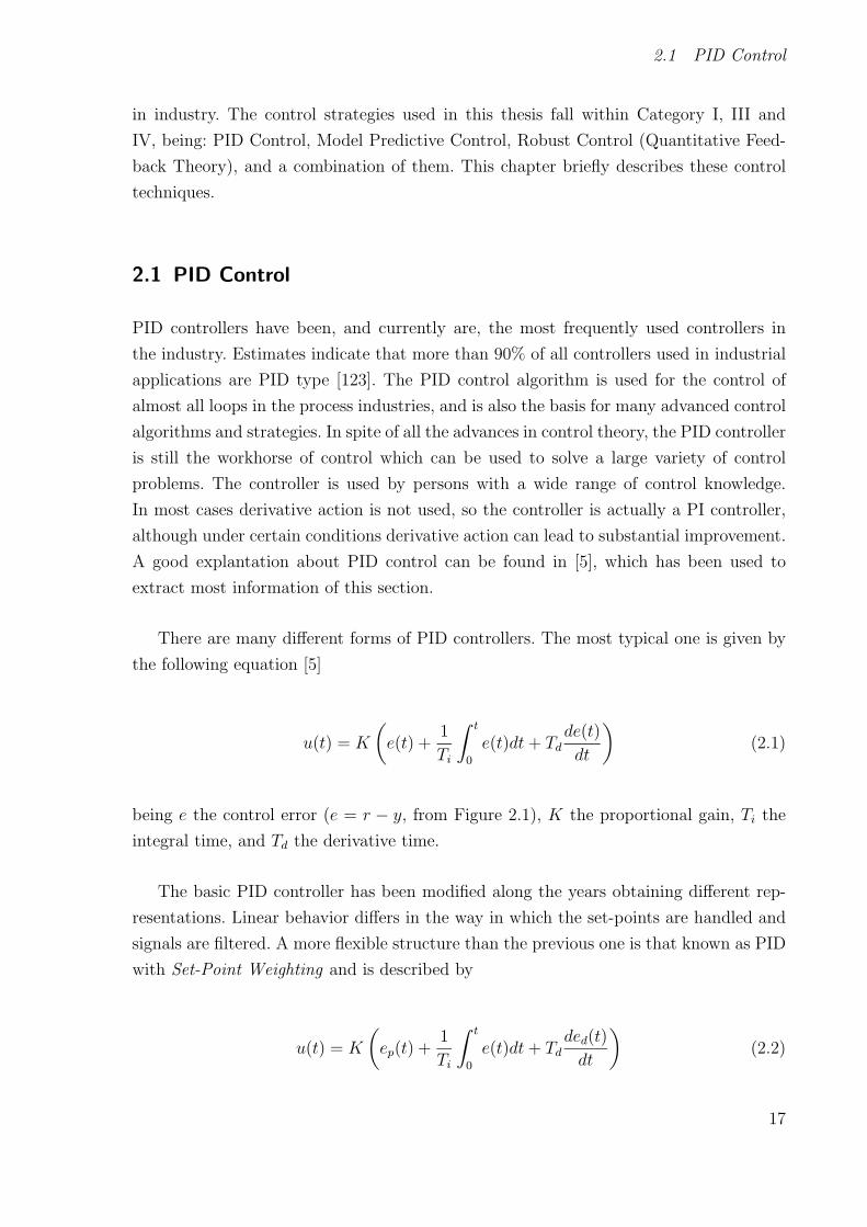
2.1 PID Control
in industry. The control strategies used in this thesis fall within Category I, III and
IV, being: PID Control, Model Predictive Control, Robust Control (Quantitative Feed-
back Theory), and a combination of them. This chapter briefly describes these control
techniques.
2.1 PID Control
PID controllers have been, and currently are, the most frequently used controllers in
the industry. Estimates indicate that more than 90% of all controllers used in industrial
applications are PID type [123]. The PID control algorithm is used for the control of
almost all loops in the process industries, and is also the basis for many advanced control
algorithms and strategies. In spite of all the advances in control theory, the PID controller
is still the workhorse of control which can be used to solve a large variety of control
problems. The controller is used by persons with a wide range of control knowledge.
In most cases derivative action is not used, so the controller is actually a PI controller,
although under certain conditions derivative action can lead to substantial improvement.
A good explantation about PID control can be found in [5], which has been used to
extract most information of this section.
There are many different forms of PID controllers. The most typical one is given by
the following equation [5]
u(t) = K
(e(t) +
1
Ti
∫ t
0
e(t)dt+ Tdde(t)
dt
)(2.1)
being e the control error (e = r − y, from Figure 2.1), K the proportional gain, Ti the
integral time, and Td the derivative time.
The basic PID controller has been modified along the years obtaining different rep-
resentations. Linear behavior differs in the way in which the set-points are handled and
signals are filtered. A more flexible structure than the previous one is that known as PID
with Set-Point Weighting and is described by
u(t) = K
(ep(t) +
1
Ti
∫ t
0
e(t)dt+ Tdded(t)
dt
)(2.2)
17

Chapter 2. Background in Automatic Control
Category I: Conventional Control Strategies
- Manual Control
- PID Control
- Ratio Control
- Cascade Control
- Feedforward Control
Category II: Advanced Control: Classical Techniques
- Gain Scheduling
- Time Delay Compensation
- Decoupling Control
- Selective/Override control
Category III: Advanced Control: Widely Used Techniques
- Model Predictive Control
- Statistical Quality Control
- Internal Model Control
- Adaptive Control
Category IV: Advanced Control: Techniques with Some Industrial Applications
- Optimal Control lqg
- Expert Systems
- Nonlinear Control
- Neural Network Controllers
- Fuzzy Control
- Robust Control
Category V: Advanced Control: Proposed Strategies with Few
(if any) Industrial Applications
Table 2.1 Process Control strategies classification by [148]
18

2.1 PID Control
where ep = br−y, ed = cr−y, and b, c are called set-point weights. So, different behaviors
for the PID controller can be obtained tuning the parameters b and c in order to face
load disturbances and measurement noise.
Another representation for the PID controller consists in the combination of filters
with the derivative term in order to reduce variations in the control signal due to high
frequency noise. The derivative term is often filtered by a first-order filter, or the ideal
derivative can also be combined with second-order filtering of the measured signal. The
transfer function of a PID controller with a filtered derivative is given by
C(s) = K
(1 +
1
sTi+
sTd1 + sTd/ℵ
)(2.3)
being C(∞) = K(1 + ℵ) the high-frequency gain. So, the ℵ parameter can be used to
reduce the variations in the control signal.
Most physical processes are constrained by several reasons, such as physical limits
(e.g. valve position), security levels (e.g. pressure levels), or performance criteria (e.g.
working near the optimal operating point). All practical PID controllers are provided
with some facility for avoiding windup of the integrator if the actuator saturates. As
well-known in the anti-windup schemes, the system remains free whereas the saturation
is not active. However, when saturation occurs, the integral term in the controller is
modified up to the system is out the saturation limit, where the modification of the
integral element is not performed instantaneously but dynamically with a time constant
Tt (see Figure 2.2)[5].
Pr(k) u(k) y(k)
+++-
u(k)
+-
iT
K
s
1
tT
1
++
K
PPr(k) u(k) y(k)
+++++-+-
u(k)u(k)
+- +-
iT
K
s
1
tT
1
++++
K
Figure 2.2 Anti-windup scheme.
Because of its wide spread use, many aspects of PID control have been developed
outside the main stream of control theory, which has had some unfortunate consequences.
There is, for example, a long continuing debate if controllers should be tuned for load
19

Chapter 2. Background in Automatic Control
disturbance response or for set-point response, an issue which is completely bypassed by
using a structure having two degrees of freedom. Set-point weighting is a simple way to
obtain the advantages of a structure with two degrees of freedom. The PID structure
used along this thesis is the following
U(s) = K
(bYsp − Y +
1
sTiE − sTd
1 + sTd/ℵ Y
), (2.4)
where U , Ysp, Y , and E are the Laplace transforms of control signal u, set-point ysp,
process output y, and control error e = ysp−y, respectively. So, it is a structure including
set-point weighting with c = 0 and filter derivative filtering which corresponds to a two
degree of freedom system with the following elements
C(s) = K
(1 +
1
sTi+ sTd
), F (s) =
bTiTds2 + (ℵTib+ Td)s+ ℵ
(ℵ + 1)TiTds2 + (ℵTi + Td)s+ ℵ (2.5)
where F (s) represents the prefilter. This structure has also a great interest from a ped-
agogical point of view. The student can begin with the typical PID structure (equation
(2.1)), and after that, the set-point weighting and noise amplification problem by the
derivative effect can be studied.
2.2 Robust Control. Quantitative Feedback Theory.
Most control techniques require the use of a plant model during the design phase in order
to tune the controller parameters. The mathematical models are an approximation of
real systems and contain imperfections by several reasons: use of low-order descriptions,
unmodelled dynamics, obtaining linear models for a specific operating point (working
with poor performance outside of this working point), etc. Therefore, control techniques
that work without taking into account these modelling errors, use a fixed-structure model
and known parameters (nominal model) supposing that the model exactly represents the
real process, and the imperfections will be removed by means of feedback. However, there
exist other control methods called robust control techniques which use these imperfections
implicity during the design phase. In the robust control field such imperfections are
called uncertainties, and instead of working only with one model (nominal model), a
family of models is used forming the nominal model + uncertainties. The uncertainties
20
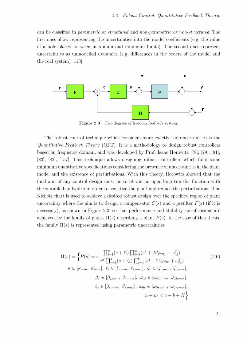
2.2 Robust Control. Quantitative Feedback Theory.
can be classified in parametric or structured and non-parametric or non-structured. The
first ones allow representing the uncertainties into the model coefficients (e.g. the value
of a pole placed between maximum and minimum limits). The second ones represent
uncertainties as unmodelled dynamics (e.g. differences in the orders of the model and
the real system) [113].
Figure 2.3 Two degrees of freedom feedback system.
The robust control technique which considers more exactly the uncertainties is the
Quantitative Feedback Theory (QFT). It is a methodology to design robust controllers
based on frequency domain, and was developed by Prof. Isaac Horowitz [78], [79], [81],
[83], [82], [157]. This technique allows designing robust controllers which fulfil some
minimum quantitative specifications considering the presence of uncertainties in the plant
model and the existence of perturbations. With this theory, Horowitz showed that the
final aim of any control design must be to obtain an open-loop transfer function with
the suitable bandwidth in order to sensitize the plant and reduce the perturbations. The
Nichols chart is used to achieve a desired robust design over the specified region of plant
uncertainty where the aim is to design a compensator C(s) and a prefilter F (s) (if it is
necessary), as shown in Figure 2.3, so that performance and stability specifications are
achieved for the family of plants Π(s) describing a plant P (s). In the case of this thesis,
the family Π(s) is represented using parametric uncertainties
Π(s) =P (s) = κ
∏ni=1(s+ i)
∏mj=1(s
2 + 2βjω0j + ω20j)
sN∏a
r=1(s+ ζr)∏b
s=1(s2 + 2βsω0s + ω2
0s): (2.6)
κ ∈ [κmin, κmax], i ∈ [i,min, i,max], ζr ∈ [ζr,min, ζr,max],
βj ∈ [βj,min, βj,max], ω0j ∈ [ω0j,min, ω0j,max],
βs ∈ [βs,min, βs,max], ω0s ∈ [ω0s,min, ω0s,max],
n+m < a+ b+N
21

Chapter 2. Background in Automatic Control
The QFT method uses the information of the plant uncertainties in a quantitative
way, imposing robust tracking, robust stability, and robust attenuation specifications
(among others). The compensator C is designed in such a way that the plant varia-
tions due to the uncertainties are inside of some specific tolerance margins, being the
perturbation effects practically imperceptible. Once this step is achieved, prefilter F is
designed in order to reach the desired reference signal. A typical QFT design involves
the following steps [20], [34]:
1. Problem specification. The plant model and the uncertainties are represented, and
the working frequencies are selected based on the system bandwidth, Ω =ω1, ω2, ...,
ωk. The specifications (stability, tracking, input disturbances, output disturbances,
noise, and control effort) for each frequency are defined, and the nominal plant P0
is selected. Table 2.2 shows the typical QFT specifications.
Specification Example of application∣∣F PCH1+PCH
∣∣ ≤ Ws1 gain and phase margins (with sensor dynamics)∣∣F 11+PCH
∣∣ ≤ Ws2 sensitivity reduction∣∣F P1+PCH
∣∣ ≤ Ws3 disturbance rejection at plant input∣∣F C1+PCH
∣∣ ≤ Ws4 control effort minimization∣∣F CH1+PCH
∣∣ ≤ Ws5 control effort (with sensor dynamics)∣∣F PC1+PCH
∣∣ ≤ Ws6 tracking bandwidth (with sensor dynamics)
Ws7, l ≤∣∣F PC
1+PCH
∣∣ ≤ Ws7, u classical 2-DOF QFT tracking problem∣∣F H1+PCH
∣∣ ≤ Ws8 disturbance rejection at plant output (with sensor dynamics)∣∣F PH1+PCH
∣∣ ≤ Ws9 rejection of plant input disturbances (with sensor dynamics)
Table 2.2 QFT specification types [20].
2. Templates. The quantitative information of the uncertainties is represented by a
set of points on the Nichols plane. This set of points is called template and defines a
graphical representation of the uncertainty at each design frequency ωi. An example
is shown in Figure 2.4, where templates of a second order system given by P (s) =Kp
s(s+a), with Kp ∈ [1, 10] and a ∈ [1, 10] are displayed for the set of frequencies
Ω = 0.5, 1, 2, 4, 8, 15, 30, 60, 90, 120, 180 rad/s.
3. Bounds. The specifications set out at the first step are traduced to prohibited
limits on the Nichols plane for the loop transfer function L(iω) = C(iω)P (iω).
These limits are known as bounds. There exist so many bounds for each frequency
as specifications are considered. So, all these bounds for each frequency are grouped
22

2.2 Robust Control. Quantitative Feedback Theory.
showing an unique prohibited bound. Figure 2.5 shows an example for stability and
tracking specifications.
Figure 2.4 QFT Template example.
4. Loop shaping. This phase consists in designing the controller elements in such a
way that the nominal loop transfer function L0(iω) = C(iω)P0(iω) is adjusted to
make the templates fulfil the bounds calculated in the previous phase. Figure 2.5
shows the design of L0 where the bounds are fulfilled at each design frequency.
Figure 2.5 QFT Bound and Loop Shaping example.
23
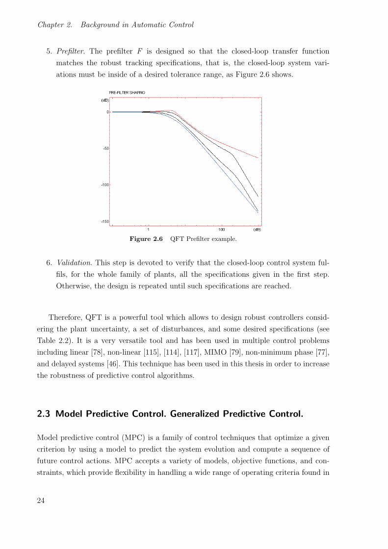
Chapter 2. Background in Automatic Control
5. Prefilter. The prefilter F is designed so that the closed-loop transfer function
matches the robust tracking specifications, that is, the closed-loop system vari-
ations must be inside of a desired tolerance range, as Figure 2.6 shows.
Figure 2.6 QFT Prefilter example.
6. Validation. This step is devoted to verify that the closed-loop control system ful-
fils, for the whole family of plants, all the specifications given in the first step.
Otherwise, the design is repeated until such specifications are reached.
Therefore, QFT is a powerful tool which allows to design robust controllers consid-
ering the plant uncertainty, a set of disturbances, and some desired specifications (see
Table 2.2). It is a very versatile tool and has been used in multiple control problems
including linear [78], non-linear [115], [114], [117], MIMO [79], non-minimum phase [77],
and delayed systems [46]. This technique has been used in this thesis in order to increase
the robustness of predictive control algorithms.
2.3 Model Predictive Control. Generalized Predictive Control.
Model predictive control (MPC) is a family of control techniques that optimize a given
criterion by using a model to predict the system evolution and compute a sequence of
future control actions. MPC accepts a variety of models, objective functions, and con-
straints, which provide flexibility in handling a wide range of operating criteria found in
24
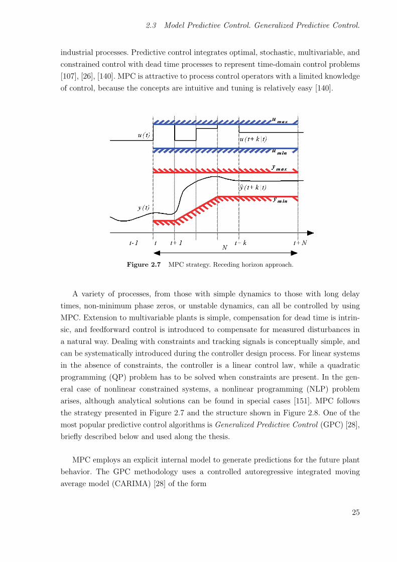
2.3 Model Predictive Control. Generalized Predictive Control.
industrial processes. Predictive control integrates optimal, stochastic, multivariable, and
constrained control with dead time processes to represent time-domain control problems
[107], [26], [140]. MPC is attractive to process control operators with a limited knowledge
of control, because the concepts are intuitive and tuning is relatively easy [140].
Figure 2.7 MPC strategy. Receding horizon approach.
A variety of processes, from those with simple dynamics to those with long delay
times, non-minimum phase zeros, or unstable dynamics, can all be controlled by using
MPC. Extension to multivariable plants is simple, compensation for dead time is intrin-
sic, and feedforward control is introduced to compensate for measured disturbances in
a natural way. Dealing with constraints and tracking signals is conceptually simple, and
can be systematically introduced during the controller design process. For linear systems
in the absence of constraints, the controller is a linear control law, while a quadratic
programming (QP) problem has to be solved when constraints are present. In the gen-
eral case of nonlinear constrained systems, a nonlinear programming (NLP) problem
arises, although analytical solutions can be found in special cases [151]. MPC follows
the strategy presented in Figure 2.7 and the structure shown in Figure 2.8. One of the
most popular predictive control algorithms is Generalized Predictive Control (GPC) [28],
briefly described below and used along the thesis.
MPC employs an explicit internal model to generate predictions for the future plant
behavior. The GPC methodology uses a controlled autoregressive integrated moving
average model (CARIMA) [28] of the form
25

Chapter 2. Background in Automatic Control
Figure 2.8 Basic MPC structure.
A(z−1)y(t) = z−dB(z−1)u(t− 1) + T(z−1)ε(t)
∆(2.7)
where u(t) and y(t) are the input and output sequences, d is the dead time, and e(t) is
a zero mean white noise. A(z−1), B(z−1), and T(z−1) are polynomials in the backward
shift operator z−1 as follows
A(z−1) = 1 + a1z−1 + a2z
−2 + · · · + anaz−na (2.8)
B(z−1) = b0 + b1z−1 + b2z
−2 + · · · + bnbz−nb (2.9)
T(z−1) = 1 + t1z−1 + t2z
−2 + · · · + tntz−nt (2.10)
This model is chosen to achieve offset-free closed-loop behavior while including non-
stationary disturbances. The polynomial T(z−1) usually equals 1 in GPC formulations.
To enhance robustness, the T− polynomial is used as a design element, which acts like a
filter to attenuate the prediction error due to high frequency unmodeled dynamics and
unmeasured load disturbances. If there are no modeling errors, the T-polynomial affects
only the disturbance rejection and not the algorithm’s setpoint tracking ability. T can
thus be used as a design parameter to increment robust stability [26], [140].
The quadratic cost function in the GPC algorithm accounts for the error between the
26

2.3 Model Predictive Control. Generalized Predictive Control.
predicted trajectory and a prescribed reference as well as the control effort. This cost
function has the form
J = EN2∑j=N1
δ(j)[y(t+ j|t) − w(t+ j)]2 +Nu∑j=1
λ(j)[∆(u)(t+ j − 1)]2 (2.11)
where E denotes expectation, y(t+ j|t) is an optimal system output prediction sequence
performed with data known up to time t, ∆u(t + j − 1) is a future control increment
sequence obtained from cost function minimization, N1 and N2 are the minimum and
maximum prediction horizons, Nu is the control horizon, and δ(j) and λ(j) are weighting
sequences that penalize the future tracking errors and control efforts, respectively, along
the horizons. The horizons and weighting sequences are design parameters used as tuning
knobs. The reference trajectory w(t+ j) can be the set-point or a smooth approximation
from the current value of the system output y(t) towards the known reference by means
of a first-order system [26].
MPC techniques enable constraints to be included in the algorithm at design stage.
As stated above, the control increments calculated by the GPC strategy are obtained by
minimizing a quadratic function of the form
J = δ(y − w)T (y − w) + λ∆uT∆u (2.12)
where usually, δ(j) = δ and λ(j) = λ for all j in the GPC cost function. The sequence
of future predictions consists in the free and forced responses
J = G∆u + f (2.13)
where the matrix G contains the system open-loop step response coefficients and f in-
cludes terms depending on present and past plant outputs and past inputs. By substi-
tuting the sequence of future outputs in
J =1
2∆uTH∆u + bT∆u + f0 (2.14)
with H = 2(δGTG+λI), bT = 2δ(f−w)TG, f0 = δ(f−w)T (f−w), the optimum solution
with no constraints is linear and given by ∆u = −H−1b. When constraints are taken into
27
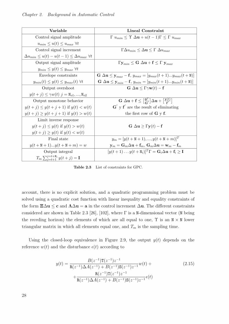
Chapter 2. Background in Automatic Control
Variable Lineal Constraint
Control signal amplitude Γ umin ≤ Υ ∆u + u(t − 1)Γ ≤ Γ umax
umin ≤ u(t) ≤ umax ∀t
Control signal increment Γ∆umin ≤ ∆u ≤ Γ ∆umax
∆umin ≤ u(t) − u(t − 1) ≤ ∆umax ∀t
Output signal amplitude Γymin ≤ G ∆u + f ≤ Γ ymaxymin ≤ y(t) ≤ ymax ∀t
Envelope constraints G ∆u ≤ ymax − f , ymax = [ymax(t + 1)...ymax(t + N)]ymin(t) ≤ y(t) ≤ ymax(t) ∀t G ∆u ≤ ymin − f , ymin = [ymin(t + 1)...ymin(t + N)]
Output overshoot G ∆u ≤ Γγw(t) − f
y(t + j) ≤ γw(t) j = No1, ..., No2
Output monotone behavior G ∆u + f ≤ [0T
G′]∆u +
[y(t)
f′]
y(t + j) ≤ y(t + j + 1) if y(t) < w(t) G′y f
′are the result of eliminating
y(t + j) ≥ y(t + j + 1) if y(t) > w(t) the first row of G y f.
Limit inverse responsey(t + j) ≤ y(t) if y(t) > w(t) G ∆u ≥ Γy(t) − f
y(t + j) ≥ y(t) if y(t) < w(t)
Final state ym = [y(t + N + 1), ..., y(t + N + m)]T
y(t + N + 1)...y(t + N + m) = w ym = Gm∆u + fm, Gm∆u = wm − fmOutput integral [y(t + 1) . . . y(t + Ni)]TΓ = Gi∆u + fi ≥ I
Tm∑j=t+Ni
j=t+1 y(t + j) = I
Table 2.3 List of constraints for GPC.
account, there is no explicit solution, and a quadratic programming problem must be
solved using a quadratic cost function with linear inequality and equality constraints of
the form Ξ∆u ≤ c and Λ∆u = a in the control increment ∆u. The different constraints
considered are shown in Table 2.3 [26], [102], where Γ is a N-dimensional vector (N being
the receding horizon) the elements of which are all equal to one, Υ is an N × N lower
triangular matrix in which all elements equal one, and Tm is the sampling time.
Using the closed-loop equivalence in Figure 2.9, the output y(t) depends on the
reference w(t) and the disturbance ε(t) according to
y(t) =B(z−1)T(z−1)z−1
R(z−1)∆A(z−1) +B(z−1)S(z−1)z−1w(t) + (2.15)
+R(z−1)T(z−1)z−1
R(z−1)∆A(z−1) +B(z−1)S(z−1)z−1ε(t)
28

2.4 Feedback properties
where
R(z−1) =T(z−1) + z−1
∑N2
j=N1kiψi∑N2
j=N1ki
, S(z−1) =
∑N2
j=N1kiMi∑N2
j=N1ki
(2.16)
Figure 2.9 GPC Closed-loop equivalence.
Here, ki are the elements of the first row of matrix (GT δG + λI)−1GT , and ψi and
Mi the polynomials of the row i in Ψ(z−1) and M(z−1), which define the free response
of the system given by [26]
f = Ψ(z−1)∆u(t− 1)
T(z−1)+M(z−1)
y(t)
T(z−1)(2.17)
Hence the characteristic polynomial for the unconstrained GPC [26], given by
ξ(z−1) = R(z−1)∆Ap(z−1) +Bp(z
−1)S(z−1)z−1 = 0, (2.18)
can be used to study the stability of GPC by calculating its roots. Ap(z−1) and Bp(z
−1)
represent the discrete transfer function of the real process. In this way the study of sta-
bility will be nominal in the case of perfect modelling (A(z−1) = Ap(z−1) and B(z−1) =
Bp(z−1)) and robust in other case.
2.4 Feedback properties
In control literature it is customary to show only responses to steps in load disturbances
or set-points. At best the control signals required to achieve the responses are also shown.
The development of H∞ theory [159] has shown that it is necessary to show at least six
29

Chapter 2. Background in Automatic Control
responses to completely characterize the behavior of a closed loop system. In [5] these
responses are refereed to as The Gang of Six and are given by
X =PCF
1 + PCR +
P
1 + PCD − PC
1 + PCN
Y =PCF
1 + PCR +
P
1 + PCD +
1
1 + PCN (2.19)
U =CF
1 + PCR− PC
1 + PCD − C
1 + PCN
where P , C and F are the transfer functions for the plant, controller and prefilter re-
spectively. R, D and N are the Laplace transforms of the reference, load disturbance,
and measurement noise, respectively; and in the same way X, Y and U represent the
Laplace transforms of the plant output without noise, plant output with noise, and the
control signal, respectively.
0 10 20 30 40 50 600
0.5
1
1.5
y
0 10 20 30 40 50 60−0.5
0
0.5
1
1.5
2
u
Figure 2.10 Basic feedback system properties. Figure from [5].
These transfer functions provide very rich information about the control system, and
they can be used to study internal stability, system robustness, the way in which the
30
2.4.1 Sensitivity functions
system reacts to load disturbances and measurement noise, as well as tracking problems.
One way to show this information can be by graphics in the form of Figure 2.10 [5].
These pictures show the response of all previous transfer functions. From them, it
is possible to observe the response of the system against set-point changes, load distur-
bances, and measurement noise. A good insight into these properties are essential for
understanding feedback systems, being a key factor in the education of any control en-
gineer [7]. All these factors in relation with The Gang of Six are discussed in depth in
[5].
2.4.1 Sensitivity functions
There are two transfer functions of the gang of six which have a great interest. These are
S =1
1 + PC, T =
PC
1 + PC(2.20)
called Sensitivity function and Complementary Sensitivity function respectively. These
transfer functions have the property that S + T = 1, and provide fundamental properties
about feedback mainly related to robustness.
The Sensitivity function S has the following properties [5]:
• It provides a robustness measurement for small process variations. For frequencies
where the sensitivity function is small the closed-loop system is very insensitive to
process variations.
• Disturbances with frequencies ω such that |S(iω)| < 1 are attenuated by feedback,
but disturbances such that |S(iω)| > 1 are amplified by the feedback.
• The maximum sensitivity value
Ms = maxω
|S(iω)| = maxω
| 1
1 + P (iω)C(iω)| (2.21)
indicates the worst-case amplification of the disturbances.
• The value sm = 1/Ms is known as the stability margin, being the shortest distance
from the Nyquist curve to the critical point -1. Hence, it can be used as a stability
indicator.
31

Chapter 2. Background in Automatic Control
On the other hand, the Complementary Sensitivity function T provides the following
information [5]:
• Robustness to large process variations can be studied using T by means of the
following expression ∣∣∣∣∆P (iω)
P (iω)
∣∣∣∣ < 1
|T (iω)| (2.22)
being assumed that the process transfer functions changes from P to P + ∆P .
• The previous upper bound can be estimated by 1/Mt being
Mt = maxω
|T (iω)| = maxω
| P (iω)C(iω)
1 + P (iω)C(iω)| (2.23)
• Large overshoot in the closed-loop response can be avoided by requiring low values
of Mt.
A graphical interpretation of these transfer functions, as well as several examples can
be found in [5]. These transfer functions together with the full gang of six will be used
in the interactive tools presented in next chapters based on PID control.
32
3
New technologies in Teaching.Interactivity
New teaching methods and innovative techniques have lately appeared showing the influ-
ences, advantages, and drawbacks that the New Information and Communication Tech-
nologies (NICT) have provided to the teaching field. Each time more and more educators
teach using new digital techniques (digital sliders, Flash animations, computer-based
simulations, etc.), providing documentation on the Internet, creating virtual forums and
courses, or performing virtual questionnaires. These great advances in the NICT have
been reflected on teaching in particular, but also in the society in general. Multiple ef-
fects can be observed at business level (remote control, remote management, flexible
timetable, etc), socio-cultural level (mobile telephone, electronic bank, digital television,
etc), and as commented above, at teaching level (digital sliders, distance education, in-
teractive information, virtual and remote labs, etc) opening an innumerable number of
possibilities [1], [108], [109], [50], [49]. From an educational point of view, the impact of
the NICT have caused the appearance of teaching techniques and methods which facil-
itate the distribution of information to the students, enhancing their motivation by the
use of new learning tools.
In a general context, the main advantages of the NICT are related with teleaccess,
teleoperation, telecontrol, and interactivity. Until recently, the exchange of information
was done using local networks by several reasons: information safety, narrow bandwidths,
limited tools for the exchange of information, etc. Due to the advances on Internet tech-
nologies, a new method for accessing the information has appeared, the teleaccess, pro-
viding a way to safely access to the information from any part of the world without
temporal constraints. Both in the industrial and research/educational fields, high costs
are often related to the restricted use of (usually expensive) systems with usage time con-
straints or to the displacements required to control them. With teleoperation (extension
of sensorial capabilities and human skill to the remote place) and telecontrol (specific
33
Chapter 3. New technologies in Teaching. Interactivity
part of teleoperation whose goal is to send commands to the actuators) technologies, it is
possible to control systems remotely through Internet, thus helping to diminish displace-
ment costs and allowing to extend the use of time-limited resources or equipment. On the
other hand, the mode in which the information is shown to the users is changing, where
data and images are not only presented as static elements, but also as interconnected
elements with some specific functionalities. This feature is known as Interactivity which
allows enhancing the users’ motivation through a more participating activity [145], [60],
[41].
In the educational field, new teaching methods have appeared related with previous
advances. These methods allow the teachers to find innovative techniques to enhance
the students motivation and improve their education: multimedia tools, hypertext sys-
tems, interactive systems, information exchange between teacher and student through
the Internet, information access from any part of the world without temporal constraints,
etc, where the biggest revolution has been produced by the World Wide Web (WWW).
All these advantages are useful for subjects without a strong practical component, but
there exist other subjects with strong experimental contents that require a new element
allowing the students to apply the acquired knowledge. Traditionally, this element has
been a local simulation tool or a local laboratory, used by the students to perform sev-
eral practical exercises over real systems but with space and time constraints. Nowadays
and thanks to advances in the NICT, especially on Internet technologies, the labora-
tory environment can be transferred to distance education. By this, two new concepts
have appeared within the distance education framework, virtual laboratories and remote
laboratories. The first of them are a new kind of simulation tools much more powerful
than the traditional ones, allowing the simultaneous use of remote simulation modules
by the students. On the other hand, remote laboratories allow the students to perform
the main laboratory activities remotely, without requiring the presence of the students
at the place where the hardware is located, in such a way that the students can control
and monitor physical devices 24 hours a day at any time and anywhere, interacting with
the teacher without having to go to the university. Remote labs help the students to put
into practice what they have learned by remotely accessing real systems [145], [60], [39].
In the same way, the presentation of information by the teachers has been improved
along the years, from the classical lectures based on blackboards and sliders to the use
of digital sliders and the providing of information through Internet. However, this fact
has considerably been improved with the appearance of Interactive Tools (IT). Although
Interactivity can be defined in several ways (as will be shown in the next section), from
34

3.1 Interactivity
a teaching point of view an IT can be defined as a collection of graphical windows whose
components are active, dynamic, and/or clickable; and that is intended to explain just a
few concepts. The use of interactive and instructional graphic tools would reinforce active
participation of students. For educators, this kind of tools can provide a very useful way
to test main ideas and to realize how difficult explaining a particular concept to students
is [143].
These advances have had, and currently have, a great impact in education. A good
example is the Automatic Control field. During the last years, teaching have received a
great attention in this field, creating the well-known Control Education area, which has
been included as a technical committee in IFAC and IEEECSS [85]. Nowadays, it is very
common to find sessions dedicated to education at the most important conferences about
control (such as IEEE Conference on Decision and Control, European Control Confer-
ence, American Control Conference, or IFAC World Congress), symposia and workshops
about control education (e.g. IFAC Symposium on Advances Control Education, or IFAC
Internet Based Control Education), related European and National projects [36], special-
ist issues about control education in the most important journals (IEEE Control System
Magazine: Innovation in Undergraduate Education, Parts I (2004)[87] and II (2005)[88],
or Control Engineering Practice: Special Section on Advances in Control Education, 2006
[89]), or even journals specifically dedicated to these issues (e.g. IEEE Transactions on
Education, Computer Applications in Engineering Education, or International Journal
of Engineering Education).
One of the main aims of this thesis is to provide contributions to Control Education
mainly focusing on interactive aspects. This chapter describes what Interactivity mean,
its application to teaching, and its impact on the Automatic Control field.
3.1 Interactivity
Interactivity in a non computer-based framework can be described as follows [126]:
Definition 1. It is some action performed mutually by two or more objects,
agents, forces, functions, etc... which allows information exchange between
each other.
35
Chapter 3. New technologies in Teaching. Interactivity
That is, the conversation between two people can be described as interactive (if both
participate into such conversation), a person driving a car is an interactive action (the
action is performed by the person and the car functionalities), or even reading a book is
also interactive in this sense (the writer interacts with the reader by means of the book).
That is, interactivity is a concept based on the well-known cause-effect relation. For some
situation being really interactive, the tasks performed by the people or objects involved
in the interactivity will produce an associated effect. A good background to understand
interactivity is to observe the daily tasks performed by people, where body and senses
perceive continuously the world interactions. On an everyday sense, when you drive you
are responding interactively with the surrounding environment and traffic. Interaction is
an accepted part of our everyday life.
Considering the previous definition, interactivity is something very common and nat-
ural. However, the use of this word by people have never been as striking as currently
is. Interactivity is a common term that people use frequently. Nowadays, it is very usual
to speak about interactive applications, interactive television, interactive mobile phones,
etc, associating the interaction between people and technological devices. The inclusion
of this phenomenon into the society has been due to the advances on the NICT. That is,
this new meaning of Interactivity comes from its use in Computer Science, where people
interact with the computer in order to perform some specific task. This definition can
be useful from a conceptual point of view, and it may seem an easy and trivial concept.
However, some complicated definitions about Interactivity can be found, such as those
related with the development of IT or graphical computer-based applications [149]:
Definition 2. It is a compromise between visual aspects, user understanding,
creativity, technical support, and direct links with the theoretical or underlying
ideas for which interactivity is required.
In the Computer Science environment, Interactivity is usually wrongly associated to
simple menu selection, clickable objects or linear sequencing. It is sometimes confused
with its original meaning based on the cause-effect relation. That is, following the origi-
nal meaning of interactivity, the simple menu selection is really interactive, but this fact
does not mean that the application including the menu is interactive. The interactive
aspects of an interface are perceived not primarily with the eye, but with our sense for
the interactive quality of things. This is not a sixth sense with dedicated sense organs,
but a faculty of human beings enabling us to perceive, judge, imagine, design, and reason
36

3.1 Interactivity
about the behavioral aspects of our environment [149]. For this reason, the development
of interactivity software can be a little bit complicated and subjective, since what a given
person perceives in a given situation is not arbitrary, but depends on the person’s ex-
pectations of what is possible. Interactivity involves a wide range of disciplines including
software engineering, computational linguistics, artificial intelligence, cognitive science
(understanding, thought, creativity), sociology, ergonomics, organizational psychology,
mathematics, cognitive psychology, and social psychology [19]. A good description to
show the difficulty associated to interactivity is described in the following definition
[153]:
Definition 3. Interactivity has gestalt properties. In the same way as you see
a rose, and not a collection of petals; hear a familiar musical theme, and not
a sequence of tones; you perceive the interactive behavior of a graphical user
interface (GUI) widget no as a collection of action/reaction pairs, but as a
meaningful interactive whole.
The inclusion of interactivity in a computer application can be seen as a fourth di-
mension. The representation of 3-D objects into a computer is currently something very
usual, corresponding to a visual component which allows to show the users wonderful
graphical representations. This fact is a very important component, but from a Com-
puter Science point of view, more important elements are required: what can i do with
this graphical element?, what kind of information can i get as feedback? That is, this
corresponds to the action component which describes the available operations to do using
a specific element. Although this matter may seem something essential, not many atten-
tion has previously put in. We live in a culture where the eye is the dominant sense, and
large investments have been made in making the GUIs around people visual appealing
[153]. Comparatively the interactive aspects of the interfaces have been less investigated.
As commented above, nowadays this fact is changing and the interactive elements are
each day more common in our society.
The implementation of interactivity can be perceived as an art because it requires a
comprehensive range of skills, including an understanding of the user, an appreciation
of software engineering capabilities, the importance of rigorous instructional design, and
the application of appropriate graphical interfaces. The term look and feel is often used
to refer to the specifications of a computer system’s interface. Using this as a metaphor,
the look refers to its visual design, while the feel refers to its interactivity. Indirectly this
37
Chapter 3. New technologies in Teaching. Interactivity
can be regarded as an informal definition of interactivity [10].
The origin of interactivity in the Computer Science field is very difficult to date. An
early effort to use interaction was made in the late 1970s by Bricklin and Frankston [23].
They developed VisiCalc, which was based on the spread sheet metaphor. It contained a
grid of rows and columns of figures for financial calculations. Its implementation on the
Apple II was one of the reasons why personal computers started to be used in the office.
VisiCalc changed spread sheet from a calculation tool to a modelling and optimization
tool. The implementation called Excel is now a standard tool in all offices. Interactive
software includes most popular programs, such as word processors or spreadsheet appli-
cations. Noninteractive programs operate without human contact such as compilers and
batch processing applications.
On the other hand, the term that can be dated is Interaction Design. This term dates
from the 80s and was developed by Bill Moggridge and his colleagues at the company
ID2 to describe their design work [155]. By focusing on interaction, the term goes to the
core of how the design of user interfaces differs from Graphics Design. As this study has
illustrated, the interactive dimension of the graphical user interface is fundamentally dif-
ferent from its visual dimension. Interactivity design can be seen as layer-based abstract
process. It begins from the idea to show using interactivity, and the first abstraction
layer is created. This process is repeated until a good abstraction is reached [153].
An explanation about the evolution of Interactive Design can be found in [39], where
such evolution is associated to the use of interactivity in the field of Automatic Control.
Design involving a human being also benefits from a fast and intuitive approach because
it lets the designer understand what is happening. Boring trial and error search from the
best set of parameters is avoided. From the control design point of view, the evolution
in the use of interactive graphics as an aid can be divided into three phases:
1. Manual calculation. This period is previous to the availability of digital computers
as a tool in the process design. The procedure consisted in the calculation of a
few numerical values. Control engineers developed sets of rules in order to draw
graphics by hand.
2. Computers as an auxiliary tool. With the advent of digital computers it was possible
to make the creation of graphics much easier. Control engineers had the possibility
of tuning the design parameters using a trial and error procedure following an
38
3.1 Interactivity
iterative process. Specifications of the problem are not usually used to calculate
the value of the system parameters because no explicit formula can connect them
directly. This is the reason for dividing each iteration, into two phases. The first
one consists in calculating the unknown parameters of the system taking a group of
design variables (related to the specifications) as a basis. During the second phase
the performance of the system is evaluated and compared to the specifications.
If they do not agree, the design variables are modified and a new iteration is
performed.
3. Computers as an interactive tool. It is possible however to merge both phases
into one, and the resulting modification in the parameters produces an immediate
effect. In this way, the design procedure becomes really dynamic and the engineers
perceive the gradient of change in the performance criteria given for the elements
that they are manipulating. This interactive capacity allows us to identify much
more easily the compromises that can be achieved.
Another important aspect related with interactivity is that, once a computer-based
application has been developed, how can its degree of interactivity be studied?. This fact
may become something subjective, and the associated interactivity could be analyzed
from several perspectives. Some interactivity features extracted by the study of several
instructional programs are outlined in [21]. In the following some recommendations from
different authors are given in order to study the interactive features of a given application:
• Immediate response means that the user is able to access information (a graph,
text, or video) with a mouse click. It is compared to the difference between face-
to-face conversation and communication through non-electronic mail. Immediate
feedback as opposed to waiting.
• Non-linear access to information. One needs to compare two models of instruction.
Model A involves a step by step hierarchical presentation of information, with no
questioning or discussion. In model B instruction responds to the level of knowledge
of each individual learner. The ability to customize the response to the user’s level
of knowledge is called adaptability.
• There is no interactivity without feedback, the user must know if the objective
has been achieved. Responses along the lines of simply ”wrong” or ”right” are not
adequate; the user needs to know how to improve and progress.
39

Chapter 3. New technologies in Teaching. Interactivity
• Adaptability and feedback should allow for a sufficient number of options. If the
users’ only option is to turn electronic pages then the program is not extracting
enough information from the user and so providing for limited instruction.
• Grain-size refers to the length of time required before allowing the user to interrupt
or initiate an action. If the user, for example, has to wait for a fifteen-minute
video or for ten minutes of credits before interaction occurs, then interactivity is
compromised.
• Learner control involves handing some degree of responsibility to the user. If the
user can control some aspects of the process such as the pace and sequence of in-
structions, then motivation and learning are likely to increase. Total learner control
is not recommended for it can lead to the too-much-rope-syndrome, an imbalance of
interactivity with the instructional focus shifting to the user. This is only beneficial
for users who are specialist in particular areas or who are generally high-achievers.
Another point of view is to study the interactivity levels which can be presented in a
specific application. In [130] three levels of interactivity are identified:
• Reactive, provides very little user control over the content with the program con-
trolling options and feedback.
• Coactive, provides user control for sequence, pace, and style.
• Proactive, allows the user to control both structure and content.
On the other hand, in [95] five levels of interactivity were identified focusing on the user’s
involvement with the program. The level of interactivity would affect whether surface or
deep learning would occur. These are:
• Modality of the learner’s response.
• The nature of the task.
• The level of processing.
• The type of program.
• The level of intelligence in design.
40

3.1 Interactivity
Finally, a last classification of interactive aspects can be performed based on the fact
that interactive concepts are not mutually exclusive events, but not elements which
can be integrated to provide comprehensive and engaging instructional transactions. In
addition, the implementation of such interactions is not only dependent on the skills of the
designers and developers, but also on the extent to which the interactions are independent
(that is, will perform identically on each encounter with a user) or consequential (where
the functionality of the interaction is dependent upon previous actions or performance
by the current user) [149]. A good context of these concepts are the following levels and
functions of interactivity
• Object interactivity (proactive inquiry) refers to an interactive program in which ob-
jects (buttons, people, things, or other metaphors) are activated by using a mouse or
other pointing devices. Clicking usually generates a form of audio-visual response.
The functionality of such objects depends on previous objects encountered, previ-
ous encounters with the current object, or previous instructional performance.
• Linear interactivity (reactive pacing) refers to functionality which allows the user
to move forwards or backwards through a predetermined linear sequence of the
content. It is often called ’electronic page-turning’. Overuse of linear interactions
in learning environments may reflect inappropriate use of technology.
• Hierarchical interactivity (reactive navigation) provides the user with a predefined
set of options from which the user can select a specific path or structure of accessing
the content. The most common example of this interaction is the main menu where
the user returns to select another option.
• Support interactivity (reactive inquiry) involves providing the user with a range
of help options and messages, some of them can be very simple and others quite
complex.
• Update interactivity relates to components of the program that initiate a dialogue
between the user and the computer-generated content. The program generates
questions or problems to which the user must respond.
• Construct interactivity is an extension of update interactivity and requires the
creation of an environment in which the user is required to manipulate component
objects to achieve specific goals.
• Reflective interactivity (proactive elaboration) refers to text responses. If n text
responses are available to the user there is always the possibility that the user will
41
Chapter 3. New technologies in Teaching. Interactivity
require the n + 1 answer and the program will judge the enquiry as ”incorrect”.
Reflective interactivity responds by providing answers recorded by other users and
allows the current user to compare and reflect on their response.
• Hyperlinked interactivity (proactive navigation) provides access to a wealth of in-
formation that the user is allowed to navigate at will. There are multiple paths
creating a ”maze” that the user needs to negotiate in order to resolve a problem.
• Non-immersive contextual interactivity (mutual elaboration) combines all previous
levels of interactivity and extends them into a complete virtual training context.
Users are transported into a microworld that reflects their existing working envi-
ronment and the tasks they undertake mirror those of their working environment.
• Immersive virtual interactivity (mutual elaboration) projects the user into a com-
plete computer-generated world which responds to individual movements and ac-
tions.
Therefore, interactivity can present multiple meanings depending on the context in which
it is defined. It can be found as something very easy and common as part of our everyday
life, as a new technological term that people use in relation to human-device interactions,
or as a more complicated element inside of the Computer Science field. In this work, inter-
activity is situated in the last context, where the interactivity influence in the teaching
field (specially in the teaching of Automatic Control concepts) will be analyzed and
developed.
3.2 Interactivity in Teaching
The use of interactivity in teaching involves the different definitions described in the pre-
vious section. In a typical lesson, the teacher must motivate the students and enhance
their participation in class, trying to obtain some feedback from the students. In the same
way, work groups may be promoted, where students can discuss and solve problems all
together exchanging ideas and information. That is, the aim is to create an interactive
environment where, as definition 1 sets, students and teachers can perform actions influ-
encing on each other. In a non-interactive lecture the teacher will talk and the students
will listen. In an interactive lecture the teacher invites questions and comments from
the students and a discussion ensues. Interactivity in learning is a necessary and funda-
mental mechanism for knowledge acquisition and the development of both cognitive and
42

3.2 Interactivity in Teaching
physical skills [10]. From this point of view, interactivity in education has two possible
ways [152]:
• Interactive teaching is a two way process wherein the teacher modifies his or her
approach in response to the needs of the students. The interactive teacher is keenly
aware of the students and their different learning styles. All good teachers are
interactive teachers. To teach effectively is not possible without interaction.
• Interactive learning is also a two way process but the student may be interacting
with the teacher, with peers, with resources, or with all three. For example, to
envisage the following key skills lesson in which the teacher aims to develop students
ability to solve problems.
Another inclusion of interactivity in teaching comes from the point of view described
by definition 3. This is also known as interactive multimedia or interactive software. These
are a new kind of computer software that mixes multimedia capabilities (text, pictures,
sound, videos, ...), together with interactive features (the multimedia elements allows
performing multiple actions and providing some kind of feedback to the user). That is,
it consists in IT with high abstraction levels allowing the teachers to show theoretical
concepts in an easier way, and the students to better understand theoretical concepts
observing their practical applications.
The theory can be learned through textbooks, inspiring lectures, and active study.
The ability to solve practical problems relies on good skill in using theory and in break-
ing down large problems into manageable subproblems. One of the important tasks for
teachers in engineering is to transmit to the students not only the formal and logic struc-
ture of the discipline, but also, and certainly with much more emphasis, the strategic and
intuitive aspects of the subject [76]. These last aspects are probably much more difficult
to make explicit and assimilate for students, precisely because they lie very often in the
less conscious substrata of the experts activity. IT are considered a great stimulus for
developing the students intuition. These IT attempt to demystify abstract mathematical
concepts through visualization for specifically chosen examples [40].
In essence, an IT is a collection of graphical windows that are manipulated by just
using the mouse. Students do not have to learn or write any sentences. If students
change any active element in the graphical windows an immediate recalculation and
43

Chapter 3. New technologies in Teaching. Interactivity
presentation automatically begins. In this way, they perceive how their modifications
affect the obtained result. IT cannot only be effective in presenting theoretical concepts
in the classroom, but also beneficial in extending student experience in analysis and
design assignments.
This strategy causes students to think small and simple. This is justified by a frank
assessment of our limited knowledge for designing educational software as well as by
practical considerations about how to manage incremental innovation. As IT are fairly
easy to create and deploy, they provide a means for rapidly prototyping and testing
theoretical ideas. In particular, they can be used as sharp tools for investigating precisely
what it takes to make a theoretical concept known to students. In this way, the virtue
of simplicity becomes an issue in learning research on the design and use of this kind of
tools [40].
In summary, the main reasons for which IT are useful for teaching are the following
[51]:
• They facilitate student-focused learning, allowing choice in the pathways for learn-
ing and the rate at which new material is introduced.
• They can address several learning styles and modalities – providing a rich variety
of instructional approaches which can teach in most of the ways what students
learn best.
• They motivate students interaction, experimentation, and cooperative learning.
• Students often work together in computer projects as they never did on paper-and-
pencil projects.
• They facilitate storylines or thematic learning – where a pathway for exploration
can easily be woven around a particular concept dynamics.
• They promote the constructivist view of learning.
However, these advantages don’t indicate that it is necessary to create IT in a discrimi-
nated way for all kind of theoretical ideas. It must be kept in mind that IT are presented
as support for the teaching. Some outlines to identify teaching problems where IT may
be suitable to use are the following [51]:
44

3.3 Warnings of Interactive Tools in Teaching
• Material which is hard to visualize, such as microscopic processes.
• Material which is three-dimensional, which is difficult to visualize using traditional
two dimensional media such as books and blackboards.
• Dynamic processes, which require an understanding of the relationships between
moving objects.
• Material which covers broad contexts, where a number of ideas need to be linked
to gain an understanding of the whole, not just the parts.
• Simulations of expensive or complex processes, where understanding may be hin-
dered by the process mechanical details, or where there is no possibility of using
real equipment.
Therefore, the presence of interactivity in teaching takes a high pedagogical value.
It is reflected at teaching methods level, in the form of interactions between teachers-
students and students-students. It is also presented as practical support, where IT help to
improve the abstraction of theoretical concepts and motivate the students’ participation.
Some results provided along this thesis are aimed on the development of IT to be used
in the teaching of Automatic Control.
3.3 Warnings of Interactive Tools in Teaching
IT can be very helpful in education but there is a danger: students try to learn and
solve problems by manipulation without understanding. The tools should challenge the
students and encouraging them to make observations and relate them to theory in order
to develop a broader and deeper understanding.
A simple view of the idea of interactive learning is that activity promotes learning.
The power of the IT sometimes provokes the user’s temptation to play with the different
dynamic objects forgetting the real meaning of such graphical elements. Teachers must
make clear to the students that IT are abstractions of the theoretical concepts, and the
full learning must be complemented as a mixture of both. In the same way that math-
ematical books are accompanied with exercises in order to understand the theoretical
concepts, IT should be used as support to the traditional lectures [53].
45

Chapter 3. New technologies in Teaching. Interactivity
However, the danger underlying in teaching with IT not only comes from the risk
that students forget the theoretical component of the subject, the great reputation that
this kind of tools are currently taking, can lead teachers to rapidly develop IT loosing
the correct abstraction levels. That is, although there exist development environments to
facilite the creation of IT (such as Sysquake [125], or Easy Java Simulations [43]), their
development requires a long time, specially during the design phase. As commented in
previous sections, the design of interactive modules can be seen as layer-based abstract
process. It begins from the idea to be shown using interactivity, and the first abstrac-
tion layer that is created. This process is repeated until a good abstraction is reached.
This fact is even more critical from an educational point of view, where the abstrac-
tion of theoretical concepts must be thought and re-thought considering the students’
perspective.
Therefore, IT can be very powerful in teaching, but they must be used with control.
3.4 Automatic Control Teaching based on Interactivity
As commented at the beginning of the chapter, during the last years the research in
the field of Automatic Control education is taking a large interest, interactivity being
one the main factors of attention [39], [41], [96], [143], [58], [53]. Several decades ago, it
was possible to find several works which have attempted to provide teaching innovations
related with interactivity. Some examples of these works are [42], [45], and [35] in which
basic IT were developed, where the interaction between the user and the computer was
mainly done by keyboard or light pen.
In the previous sections, abstraction has been set as one of the most important
features for IT. In this context, abstraction refers to associate theoretical concepts with
graphical elements. That is, visualizing the concepts with graphical and dynamic pictures.
This is known as visualization, which was defined in the Introduction chapter. A good way
to understand it can be found in [41], where the following story illustrates better than any
analysis what visualization is. The anecdote usually has Norbert Wiener as protagonist,
but there are many control engineering students who would be able to recognize the
same attitude in some, or perhaps many, of the teachers that they have had throughout
the course of their studies. Wiener was developing a complicated demonstration in front
of his class at MIT. The blackboard was full to overflowing with intricate formulae.
Suddenly, he got stuck; he stared at the last formula and became statue-like for a good
46

3.4 Automatic Control Teaching based on Interactivity
while. Everyone gasped as they thought he was in a jam. Yet, Wiener, without uttering a
single word, went to the corner of the blackboard where there was a bit of space left and
drew some figures that no one could see because his back was hiding them from view.
Suddenly, his face lit up. Without uttering a single word he rubbed off his mysterious
figures and went back to the point where he had got stuck, and continued faultlessly to
the end without any problem.
In order to design technical systems or simply to understand the physical laws that
describe their behavior, scientists and engineers often use computers to calculate and
graphically represent different magnitudes. In control engineering, these quantities in-
clude among others: time and frequency responses, poles and zeros on the complex plane,
Bode, Nyquist and Nichols diagrams, phase plane, etc. Frequently these magnitudes are
closely related and constitute different visions of a single reality. The understanding of
these relationships is one of the keys to achieve a good learning of the basic concepts
and it enables students to accurately design control systems [39].
Automatic control ideas, concepts, and methods are really rich in visual contents
that can be represented intuitively and geometrically. These visual contents can be used
for presenting tasks and handling concepts and methods, and manipulated for solving
problems. Control specialists have visual images, intuitive ways of perceiving concepts
and methods that are exceedingly important for effectively carrying out their creative
work and mastering the field in which they work. Using visual images and intuition,
they are able to relate constellations of facts that are frequently highly complex, and the
results of their theories in an extremely versatile and varied way. Furthermore, via these
significant networks, they are able to naturally and effortlessly choose the most effective
strategies to attack and solve the problems facing them [41].
The basic ideas of automatic control often arise from very specific and visual situ-
ations. All experts know how useful it is to go to this specific origin when they want
to skilfully handle the corresponding abstract objects. The same occurs with other ap-
parently more abstract parts of Automatic Control. This way of acting with explicit
attention to potential specific representations to explain the abstract relations that are
of interest to the control expert is what we name control visualization.
The fact that visualization is an especially important aspect in the control experts
activity is something completely natural if we bear in mind the applied mathematics
feature of control theory. Broadly speaking, mathematics tries to explore the structures
47

Chapter 3. New technologies in Teaching. Interactivity
of the reality that are accessible using this special manipulation that we call mathema-
tisation, which could be described as follows. The first perception is that tangible things
have certain similarities and we recognize from these perceptions what is common and
can be abstracted. We then subject this information to rational and symbolic detail in
order to handle more clearly the underlying structure of these perceptions [41].
People feeling is primarily visual and it is thus not surprising that visual support is
so present in the daily work. Control experts very often make use of symbolic processes,
visual diagrams, and other forms of imaginative processes in their work and they acquire
what could be called an intuition of what is abstract. Visualisation thus appears to be
something deeply natural both in the origins of automatic control and the discovery
of new relations between mathematical objects, and also of course in the transmission
and communication of our control knowledge. One of the important tasks for teachers
in control engineering is to transmit to students not only the formal and logic structure
of our discipline but also, and certainly with much more emphasis, the strategic and
intuitive aspects of the subject. These strategic and intuitive aspects are probably much
more difficult to make explicit and assimilate for students, precisely because they are
very often in the less conscious substrata of the experts activity. Given the nature of
visualization, it will have many highly subjective elements [41].
The ways of visualizing and making Automatic Control ideas closer and intuitive
in order to implement them in certain situations, and apply them to specific problems,
depends a lot on each individuals mental structure. The degree of visual support certainly
varies considerably from one analysis to another, and what for a person is helpful, for
another person is possibly a hindrance. Yet, these differences must not hamper our
attempts to generously offer those instruments that are so useful for us in our work
and without which our work would be much more difficult, abstruse, and boring. The
mathematical language used by control specialists is a mixture of natural language and
formalised language, a strange jargon consisting of natural language elements, more or
less esoteric words, and logical and mathematical symbols. In this strange language
reference is explicitly made, or not so explicitly, to scientific conventions that have been
established in the course of time and that are laden with intuitive, visual, and implicit
connotations. It is not surprising that mathematical and communication work using this
tool produces mistakes, confusion, and obscurities that may lead to error.
According to [150], a control designer (teacher, engineer, or student) must fulfill the
following procedure in order to design a suitable control system for a plant [143]:
48

3.4 Automatic Control Teaching based on Interactivity
1. Study the plant to be controlled and obtain initial information about the control
objectives.
2. Model the plant and simplify the model, if necessary.
3. Analyze the resulting model; determine its properties.
4. Decide which variables are to be controlled (controlled outputs).
5. Select the control configuration.
6. Decide on the type of controller to be used.
7. Decide on performance specifications, based on the overall control objectives.
8. Design a controller.
9. Analyze the results and if the specifications are not satisfied, modify it or the type
of controller.
10. Simulate the resulting controlled system, either on a computer or pilot plant.
11. Repeat from step 2, if necessary.
12. Choose hardware and software and implement the controller.
13. Test and validate the control system, and tune the controller on line, if necessary.
It can be observed that if the design of the control system leads to unsatisfactory
results of the simulations (step 10), it would be forced to go back to step 2 and proceed
to repeat steps 2 to 10, analyzing them one-by-one. The previous approach to design a
control system using traditional tools can be considered a non-interactive approach (see
Figure 3.1(a)). This is due to the fact that it is not possible to know the consequences of
the decisions taken during the design process until we are very near the end (step 11),
just before the final hardware implementations. This situation produces that the same
steps must be repeated over and over in order to correctly tune the design parameters,
making this a very time-consuming activity. This is a direct consequence of the non-
existence of a real-time link between the design and the analysis phases, avoiding the
designer from appreciating the gradient of change in the performance criteria given for
the elements he/she is manipulating [143].
If there were such a real-time connection or link between the decisions taken during
the design phase and the results obtained in the analysis phase, both phases could be
49

Chapter 3. New technologies in Teaching. Interactivity
SynthesisSynthesis
AnalysisAnalysis
SynthesisSynthesis
AnalysisAnalysis
SynthesisSynthesis
++
AnalysisAnalysis
SynthesisSynthesis
++
AnalysisAnalysis
(a) Non-Interactive approach (b) Interactive approach
Figure 3.1 Non-Interactive approach versus Interactive approach.
merged into one. In this new approach, decisions taken in some steps would show on-the-
fly the differences between the simulation results and the original control specifications
fixed in step 1. It would not be necessary to iterate so many times across every step
trying to tune the parameters. But this proposed link to merge analysis and design
can be brought to existence giving interactivity the central role that it deserves in the
development of new software tools for control education. So, this would be an interactive
approach (see Figure 3.1(b)).
In such a high-interactive system, several graphic windows are updated immediately,
reflecting the value of every active element, and the constraints among them. This lets
us establish a reactive behavior among all active components of the system, hiding the
underlying mathematical basis. Every change in the values of system parameters has a
dynamic effect on the system response. Since a good design usually involves multiple
control objectives using different representations (time domain or frequency domain), it
is possible to display several graphic windows that can be updated simultaneously during
the manipulation of the active elements [143], [41]. Furthermore, interactive design with
instantaneous performance display let us go further. In many cases, it is not only possible
to calculate the position of a graphic element (be it a curve, a pole, or a template) from
the model, controller, or specifications, but also calculate a new controller from the
position of the element. For instance, a closed loop pole can be computed by calculating
the roots of the characteristic polynomial, itself based on the model and controller; and
the controller parameters can be synthesized from the set of closed loop poles if some
conditions on the degrees are fulfilled [32].
50

3.4 Automatic Control Teaching based on Interactivity
Many tools for control education have been developed over the years incorporating the
concepts of dynamic pictures and virtual interactive systems [156]. Nowadays a new gen-
eration of software packages has appeared, based on objects that admit a direct graphic
manipulation and that are automatically updated, so that the relationship among them
is continuously maintained. The early programs were useful but their implementation
required a substantial effort which significantly limited their use in education. Advances
in computers and software have made implementation easier. Matlab has been used in
several projects, where two successful efforts have resulted in ICTools [94] and CCSdemo
[156] developed in the Department of Automatic Control at Lund Institute of Technol-
ogy. The programs are, however, strongly version dependent which has made support and
future development cumbersome. Yves Piguet at the Federal Institute of Technology in
Lausanne (EPFL) developed a Matlab-like program Sysquake which has strong support
for interactive graphics [125]. Projects based on Sysquake were developed at EPFL and
elsewhere (see [58], [53], [38], [33]).
Therefore, the role of this new interactive computer learning experience in control
engineering curriculum is twofold [39]:
• To provide a new method for delivering classroom material whereby real-world
control system engineering concepts are introduced via an interactive package, and
• to provide an opportunity for innovative laboratory assignments where students
can analyze, design, and modify control engineering systems via IT.
The combinations of an interactive environment plus animation bring visualization
to a new level and aid learning, and active participation by control engineering students.
Automatic Control teachers are at the threshold of a new era in which advanced informa-
tion technology is finding its way towards effective and efficient applications in control
education [97].
51


4
Interactive Tools for PID Control
The idea of changing properties and immediately being able to see the effects is very pow-
erful both for learning and for designing in the Automatic Control field. As described in
chapter 2, in spite of all the advances in control theory, the PID controller is still the
workhorse of control which can be used to solve a large variety of control problems. So,
this chapter describes three interactive learning modules which have been developed to
permit obtaining a good intuition and working knowledge of PID control. The design of
the modules was developed considering all common aspects with the aim of performing
similar structured interfaces. The modules consist of menus where process transfer func-
tions and PID controllers can be chosen, parameters can be set, and results stored and
loaded. A graphic display which shows time or frequency responses is a central part. The
graphics can be manipulated directly by dragging points, lines, and curves or by using
sliders. Parameters that characterize robustness and performance are also displayed. All
modules have two icons to access Instructions and Theory. Instructions give access to a
document which contains suggestions for exercises, and Theory provides access to rele-
vant theory via Internet. The modules can be used in many different ways, one extreme
is a full-fledged exercise with serious analysis and reporting, another is simply free ex-
perimentation following own ideas. The modules can be used in lectures and, as will be
shown in the next sections, multiple exercises can be proposed to give a good intuitive
understanding of the properties of PID Control.
These modules were obtained as result of a research stay at the Lund Institute of
Technology (Sweden). They were developed under a strong collaboration and supervi-
sion of professors Karl Johan Astrom and Tore Hagglund, where the modules can be
viewed as an attempt to make the key pictures in the book Advanced PID Control [5]
interactive. The idea was to develop interactive learning tools which could be used for
introductory control courses at universities and other schools, and for engineers in in-
dustry. The modules should be self-contained, suitable both for self-study, courses, and
for demonstrations in lectures, and they should not require any additional software. At
53

Chapter 4. Interactive Tools for PID Control
present there are more modules under development, and in the future it will be pos-
sible to have more than nine evolving modelling, model reduction, PID design, Smith
predictor, coupled loops and feedforward.
The modules are implemented in Sysquake [125], a Matlab-like language with fast
execution and excellent facilities for interactive graphics. The modules are free and avail-
able on the web at http://www.calerga.com for Windows, Mac, and Linux operating
systems.
The implementation of the modules is reasonably straight forward. Manipulation of
graphical objects are well supported in Sysquake. Numerics for simulation consist of
solving linear differential equations with constant coefficients and simple nonlinearities
representing the saturations. For linear systems the complete system is sampled at con-
stant sampling rate and the sampled equations are iterated. For systems with saturation
the process and the controller are sampled separately with first order holds, the non-
linearities are added, and the difference equations are then iterated. Delays are simply
dealt with because the sampled systems are difference equations of finite order.
The numerical calculations for loop shaping are simply manipulation of complex
numbers. In this case, a more general classes of systems are dealt with by using symbolic
representations of functions. The transfer function P (s) = 1/ cosh√s can be represented
as P=’1/cosh(sqrt(s))’. In the plots the loop transfer function for complex arguments
has to be evaluated which is done in the following way:
w=logspace(-2,2,500);
s=i*w;
P=’1/cosh(sqrt(s))’;
Pv=eval(P);
In this way systems that are described by partial differential equations can be represented.
Next sections describe the three developed modules: the central module is called PID
Basics, two auxiliary modules PID Loop Shaping and PID Windup illustrate loop shaping
and windup [53]. One consideration that must be kept in mind is that the main feature
of the tools (Interactivity) cannot be easily illustrated in a written text. Nevertheless,
some of the advantages of the applications are shown. The author cordially invite to visit
the web site to experience the interactive features of the tools [53].
54

4.1 PID Basics
4.1 PID Basics
A simple and intuitive way to understand PID control is to look at the responses of the
closed-loop system in the time domain and to observe how the responses depend on the
controller parameters. As commented in chapter 2, in order to have a reasonably complete
understanding of a feedback loop, it is essential to consider six responses, the Gang of Six
[5]. One possibility is to show process output and controller output for step commands
in set-point and load disturbances, and the response to noise in the sensor. The study
of feedback in this way can be performed using PID Basics. Frequency responses and
mixed time and frequency results can also be shown.
The interaction is straight forward because it is done mainly by using sliders for
controller parameters. Process models can be chosen from a menu which contains a wide
range of transfer functions. It is also possible to enter an arbitrary transfer function
in the Matlab rational function format. Process gain and time delay can be changed
interactively. The PID controller has the structure represented by (2.4).
4.1.1 Description of the Interactive Tool
This section briefly describes the main aspects of PID Basics. The main screen of the
tool is shown in Figure 4.1.
Process
It corresponds to the parameter group located on the left hand side of the tool screen,
just below the icons (see Figure 4.1). It contains the information about the process to
control, showing a symbolic representation of the transfer function and several interactive
elements to change the process parameters. From Figure 4.1 it can be seen that the
current example is a fourth order process with the transfer function
G(s) =Kp
(s+ 1)n
where the interactive parameters are given by Kp (by means of a slider) and n (by means
of a text edit). When the user modifies any plant parameter, the symbolic representation
is immediately updated, being its effect reflected on the rest of IT elements. The user
can modify the transfer function of the process from the Settings menu as will be shown
later.
55

Chapter 4. Interactive Tools for PID Control
Figure 4.1 The user interface of the module PID Basics. The plots show the time responseof the Gang of Six.
Controller
Five radio buttons are available to select the desired controller. The options to choose
are proportional (P), integral (I), proportional-integral (PI), proportional-derivative (PD),
and proportional-integral-derivative (PID). Several sliders are available below the radio
buttons in order to modify the controller parameters. The number of sliders shown de-
pends on the chosen controller. For example, Figure 4.1 shows five sliders since the option
selected is a PID controller (K, Ti, Td, ℵ, and b).
Performance and robustness information
Some measures about performance and robustness are provided in order to study the con-
trol designs. The performance category is classified into three groups: set-point response,
load disturbances, and noise response. For the set-point response the integral absolute
error (IAE) and overshoot (overshoot) measures are given. Integral absolute error (IAE),
integral gain (ki), maximum error (emax), and the time to reach the maximum (tmax)
are the information provided for load disturbances. The integral absolute errors and the
56

4.1.1 Description of the Interactive Tool
maximum error values are normalized to unit step changes in setpoint and load distur-
bances. The response to noise is characterized by the standard deviations of the signals
x (signal without noise, sigma x), y (signal with noise, sigma y), and u (control signal,
sigma u). The robustness measures are maximum sensitivity (Ms), maximum comple-
mentary sensitivity (Mt), gain margin (Gm), and phase margin (Pm). This information
can be duplicated in order to compare two designs as will be shown later. A deeper
description of these measures can be found in reference [5].
Graphics
A couple of graphics are shown on the right hand side of the tool (see Figure 4.1). These
graphics have three representation modes depending on the selected option from Settings
menu. These modes are time domain, frequency domain, and frequency/time domain.
The time domain mode is that shown in Figure 4.1, where the time responses for the
system output (Process Output) and input (Controller Output) are displayed, so providing
all the information evolved in the Gang of Six [5]. There are several interactive graphical
elements on the graphics to interact with the application. The vertical green line located
at time t = 0 allows modifying the set-point amplitude. The green and black vertical lines
located in the middle of the graphics allow setting the value and instant time for load
disturbances and measurement noise respectively. The vertical and horizontal scales can
be modified using three black triangles available on the graphics (, ). For example, in
Figure 4.1 the set-point is set to 1, the load disturbance to 0.9 at instant time 32, and
the measurement noise to 0.02 at instant time 60. It is also possible to know the value for
the input or output signal at an specific instant time, being only necessary to place the
mouse over the curve. Figure 4.1 shows an example where for the instant time t = 37.78,
the output and input signals are 1.62 and 0.38 respectively. Notice that all the previous
options are available from both graphics, Process Output and Controller Output.
On the top of the Process Output graphic, there are two checkboxes called save and
delete. These buttons make it easy to store a simulation for comparison. If the save
button is selected, the current design is saved and kept on the graphics in blue color.
Then, a new design in red color appears allowing to perform a comparison between both
designs. Performance and robustness parameters are duplicated showing the values in
red and blue colors associated to each design. Legends at Process Output and Controller
Output graphics are also shown with the value of controller parameters for both designs.
Figure 4.1 shows an example which compares response of PI (K = 0.43, Ti = 2.27, b = 0)
and PID (K = 1.13, Ti = 3.36, Td = 1.21, b = 0.54, ℵ = 10) controllers for a process
57
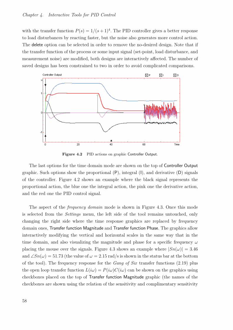
Chapter 4. Interactive Tools for PID Control
with the transfer function P (s) = 1/(s+ 1)4. The PID controller gives a better response
to load disturbances by reacting faster, but the noise also generates more control action.
The delete option can be selected in order to remove the no-desired design. Note that if
the transfer function of the process or some input signal (set-point, load disturbance, and
measurement noise) are modified, both designs are interactively affected. The number of
saved designs has been constrained to two in order to avoid complicated comparisons.
Figure 4.2 PID actions on graphic Controller Output.
The last options for the time domain mode are shown on the top of Controller Output
graphic. Such options show the proportional (P), integral (I), and derivative (D) signals
of the controller. Figure 4.2 shows an example where the black signal represents the
proportional action, the blue one the integral action, the pink one the derivative action,
and the red one the PID control signal.
The aspect of the frequency domain mode is shown in Figure 4.3. Once this mode
is selected from the Settings menu, the left side of the tool remains untouched, only
changing the right side where the time response graphics are replaced by frequency
domain ones, Transfer function Magnitude and Transfer function Phase. The graphics allow
interactively modifying the vertical and horizontal scales in the same way that in the
time domain, and also visualizing the magnitude and phase for a specific frequency ω
placing the mouse over the signals. Figure 4.3 shows an example where |Sn(ω)| = 3.46
and ∠Sn(ω) = 51.73 (the value of ω = 2.15 rad/s is shown in the status bar at the bottom
of the tool). The frequency response for the Gang of Six transfer functions (2.19) plus
the open loop transfer function L(iω) = P (iω)C(iω) can be shown on the graphics using
checkboxes placed on the top of Transfer function Magnitude graphic (the names of the
checkboxes are shown using the relation of the sensitivity and complimentary sensitivity
58

4.1.1 Description of the Interactive Tool
Figure 4.3 Frequency domain mode.
functions with the rest of transfer functions. e.g. PS = P 11+PC
). Figure 4.3 shows an
example where all transfer functions are shown.
It is also possible to show time and frequency domains simultaneously. An example
can be seen in Figure 4.4. The upper graphic represents time domain, and the lower one
represents frequency domain. The default screen shows the output and the magnitude
for the time and frequency domains, respectively. However, on the top of the graphics,
there exists a couple of radio buttons which permit choosing between the output or input
(for time domain), and magnitude or phase (for frequency domain). This mode is very
interesting since it is possible to observe the effect of parameter modifications on both
domains simultaneously.
Settings menu
The Settings menu is available on the top menu of PID Basics, and it is divided into
six groups as Figure 4.5 shows. From the first entry, Process transfer function, several
processes can be selected, being also available an option to enter an arbitrary transfer
59

Chapter 4. Interactive Tools for PID Control
Figure 4.4 Time and Frequency domains simultaneously.
Figure 4.5 Settings menu for PID Basics.
function in the numerator (num) and denominator (den) form used in Matlab. Specific
values for controller parameters can be entered using the Controller parameters menu op-
tion. The third entry, Time/Frequency domain, allows choosing between the three modes
commented above: Time domain, Frequency domain, and Both domains. Results can be
stored and recalled using the Load/Save menu (using the options Save design and Load
design respectively). The option Save report helps to save all essential data in ascii format,
this possibility being useful for documenting results. The menu selection Simulation fits
the simulation time, the maximum time delay (in order to avoid slow simulations), and
to active the Sweep option to show the results for several controller parameters simul-
60
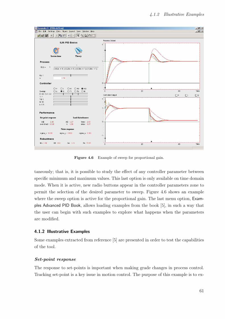
4.1.2 Illustrative Examples
Figure 4.6 Example of sweep for proportional gain.
taneously; that is, it is possible to study the effect of any controller parameter between
specific minimum and maximum values. This last option is only available on time domain
mode. When it is active, new radio buttons appear in the controller parameters zone to
permit the selection of the desired parameter to sweep. Figure 4.6 shows an example
where the sweep option is active for the proportional gain. The last menu option, Exam-
ples Advanced PID Book, allows loading examples from the book [5], in such a way that
the user can begin with such examples to explore what happens when the parameters
are modified.
4.1.2 Illustrative Examples
Some examples extracted from reference [5] are presented in order to test the capabilities
of the tool.
Set-point response
The response to set-points is important when making grade changes in process control.
Tracking set-point is a key issue in motion control. The purpose of this example is to ex-
61
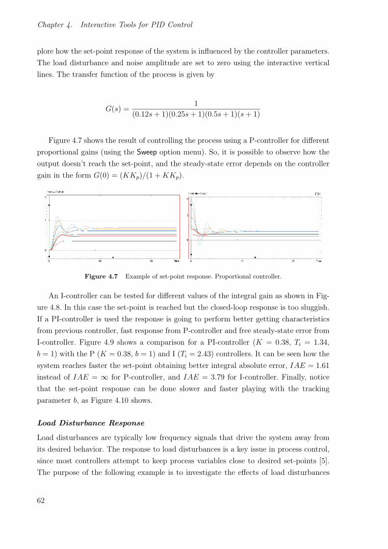
Chapter 4. Interactive Tools for PID Control
plore how the set-point response of the system is influenced by the controller parameters.
The load disturbance and noise amplitude are set to zero using the interactive vertical
lines. The transfer function of the process is given by
G(s) =1
(0.12s+ 1)(0.25s+ 1)(0.5s+ 1)(s+ 1)
Figure 4.7 shows the result of controlling the process using a P-controller for different
proportional gains (using the Sweep option menu). So, it is possible to observe how the
output doesn’t reach the set-point, and the steady-state error depends on the controller
gain in the form G(0) = (KKp)/(1 +KKp).
Figure 4.7 Example of set-point response. Proportional controller.
An I-controller can be tested for different values of the integral gain as shown in Fig-
ure 4.8. In this case the set-point is reached but the closed-loop response is too sluggish.
If a PI-controller is used the response is going to perform better getting characteristics
from previous controller, fast response from P-controller and free steady-state error from
I-controller. Figure 4.9 shows a comparison for a PI-controller (K = 0.38, Ti = 1.34,
b = 1) with the P (K = 0.38, b = 1) and I (Ti = 2.43) controllers. It can be seen how the
system reaches faster the set-point obtaining better integral absolute error, IAE = 1.61
instead of IAE = ∞ for P-controller, and IAE = 3.79 for I-controller. Finally, notice
that the set-point response can be done slower and faster playing with the tracking
parameter b, as Figure 4.10 shows.
Load Disturbance Response
Load disturbances are typically low frequency signals that drive the system away from
its desired behavior. The response to load disturbances is a key issue in process control,
since most controllers attempt to keep process variables close to desired set-points [5].
The purpose of the following example is to investigate the effects of load disturbances
62

4.1.2 Illustrative Examples
Figure 4.8 Example of set-point response. Integral controller.
(a) P vs PI control (b) I vs PI control
Figure 4.9 Example of set-point response. PI controller.
Figure 4.10 Example of set-point response. Effect of b parameter.
and how their effect is influenced by the controller type and parameter settings. The
set-point and noise amplitudes haven been set to zero, and the amplitude of the load
disturbance has been set to 0.9 at instant time t = 0. The process transfer function is
given by
63

Chapter 4. Interactive Tools for PID Control
G(s) =1
(s+ 1)4
Firstly, a comparison between a P-controller (K = 0.6, b = 1) and PI-controller
(K = 0.6, Ti = 2, b = 1) is displayed in Figure 4.11. It can be observed how the P-
controller doesn’t eliminate the effect of the disturbances, while the PI-controller does.
This fact can be corroborated from the transfer function Gyd = YD
= P1+PC
, where for a
P-controller that Gyd(0) = K1+KKp
0, and for a PI-controller Gyd(0) = 0.
Figure 4.11 Example of load disturbance response. P and PI controllers.
So, as commented above, the response of the process variable to load disturbances is
given by [5]
Gyd =P
1 + PC= PS =
T
C
For a system with P (0) = 0 and a controller with integral action the previous transfer
function can be approximated by [5]:
Gyd =T
C≈ 1
C≈ C
ki
where ki = KTi
is the integral gain. Since load disturbances typically have low frequencies
the previos equation is a good measure of load disturbance rejection. So, large values of
ki will provide adequate load disturbance responses.
Figure 4.12 shows the load disturbance responses for two PI controllers with ki values
of 0.36 (in red color) and 0.30 (in blue color). As the previous equation indicates, the
64

4.1.2 Illustrative Examples
controller with bigger integral gain leads to better results to load disturbances, obtaining
a faster response and smaller values for IAE and emax, but the stability margins are
reduced, as can be observed from the robustness parameters. Figure 4.13 shows the
frequency responses of Gyd and S for two PI controllers with large (ki = 0.85) and small
(ki = 0.30) values of ki. From this figure, it can be noticed that large values of ki imply
large peaks of the sensitivity function. So, it is necessary to reach a trade-off between
load disturbance rejection and robustness.
Figure 4.12 Example of load disturbance response. Integral gain (ki) influence.
Figure 4.13 Example of load disturbance response. Frequency domain responses of Gyd andS for a PI with ki = 0.85 (left) and ki = 0.30 (right).
Some tuning methods allow obtaining good compromises between robustness and load
disturbance response. AMIGO (Approximate M constrained Integral Gain Optimization)
[5], [72], [73], [74] is one of these methods that, in the same way that the well-known
Ziegler and Nichols method [162], [163], focusses on load disturbances by maximizing
integral gain but also adding a robustness constraint. For the previous example, the
result of applying this method is shown in Figure 4.14. The AMIGO-step method has
65

Chapter 4. Interactive Tools for PID Control
Figure 4.14 Example of load disturbance response. PI controller using AMIGO-step method.
been used to design a PI controller with K = 0.414 and Ti = 2.66. A slow response to
load disturbances is obtained but with good stability margins.
Response to measurement noise
Measurement noise is a disturbance that distorts the information about the process
obtained by the sensors. Measurement noise typically has high frequencies, and is fed
into the system by feedback. This phenomenon creates control actions and variations in
the process output, being important that measurement noise does not generate too large
control actions. The next example shows how measurement noise affects the system and
how this influence can be reduced [5]. The process transfer function is given by
G(s) =1
(0.01s+ 1)(0.04s+ 1)(0.2s+ 1)(s+ 1)
Figure 4.15 shows a simulation for two PID controllers where the measurement noise
has been set to 0.02, and the set-point and load disturbance amplitudes to zero. A PID
controller with K = 1, Ti = 1, Td = 0.9, b = 0.5, and ℵ = 10 is represented in red
color. As seen, large control actions are obtained for this controller. This performance
can be improved increasing the filtering effect (as commented in chapter 2). So, the same
controller is used but the ℵ parameter is reduced to 1.5, showing the results in blue color.
From the figure it can be observed how the control action variations are considerably
reduced, remaining the system output practically unalterable.
66

4.1.2 Illustrative Examples
Figure 4.15 Example of measurement noise response. PID controllers with ℵ = 1.5 andℵ = 10.
The previous results can be corroborated from the gang of six transfer functions
(2.19). The transfer function which relates the control signal with the measurement
noise is given by
Gun =C
1 + PC= CS =
T
P
where, as measurement noise typically has high frequencies, this transfer function can be
approximated by Gun = C. So, for a classical PID controller (2.1), at high frequencies
|Gun| becomes infinite due to the derivative term, which clearly indicates the necessity
of filtering the derivative term. This fact can be tested for the previous time domain
example, using the frequency domain mode in PID Basics. A simple index of the effect
of measurement noise is the largest gain of the transfer function Gun [5]
Mun = maxω
|Gun(iω)|
Figure 4.16 shows the frequency responses of |Gun| for the previous two controllers
with ℵ = 10 and ℵ = 1.5. The magnitude is considerably reduced for ℵ = 1.5 being the
maximum value ≈ 3, whereas for ℵ = 10 the maximum magnitude is ≈ 11.
Figure 4.16 Example of measurement noise response. Frequency domain interpretation forℵ = 10 (left) and ℵ = 1.5 (right) using the transfer function Gun = C/(1 + PC).
67

Chapter 4. Interactive Tools for PID Control
More examples
Many other examples can be developed using the tool from the time and frequency do-
mains point of view. For instance, examples 7.1 (lag-dominated dynamics), 7.2 (balanced
lag and delay) and 7.3 (delay-dominated dynamics) of the reference [5] can be loaded
and studied from the Settings menu. Examples about delayed system and robustness can
also be performed using PID Basics. Some of them will be shown using the next tool in
the loop shaping context.
4.2 PID Loop Shaping
There are many interesting issues that have to be dealt with when developing IT for
control which are related to the particular graphics representations used. It is straight
forward to see the effects of parameters on the graphics but not so obvious how the
graphical objects should be manipulated. There are natural ways to modify pole-zero
plots, for example by adding poles and zeros and by dragging them. Bode plots can
be manipulated by dragging the intersections of the asymptotes. Nevertheless, it is less
obvious how a Nyquist plot should be changed. The tool presented in this section, called
PID Loop Shaping, shows the Nyquist plots of the process transfer function P (s) and
the loop transfer functions L(s) = P (s)C(s) (see Figure 4.17).
4.2.1 Description of the Interactive Tool
This section describes briefly the different elements of PID Loop Shaping and some easy
theoretical aspects.
Process
This description of PID Loop Shaping is very similar to the PID Basics one. However, the
process transfer function is presented as a pole-zero interactive graphic in the s-plane
instead of a symbolic representation. The process transfer function can be modified
depending on the option selected from the Settings menu. Several examples of transfer
function are available, and its parameters can be modified using sliders as in PID Basics.
However, a free transfer function can be selected (Interactive TF menu option), where
poles and zeros can be defined graphically as Figure 4.17 shows.
Controller
This zone of the tool shows the different parameters and capabilities of PID Loop Shaping
in order to perform loop shaping. Loop shaping is a design method where a controller
68

4.2.1 Description of the Interactive Tool
Figure 4.17 The user interface of the module PID Loop Shaping, showing both Free andConstrained PID tuning.
is chosen such that the loop transfer function reaches the desired shape. The key idea
is that the action of the controller can be interpreted as mapping the process Nyquist
plot to the Nyquist plot of the loop transfer function. This mapping is performed to
an specific design frequency ω. This frequency determines the desired point to move on
the process transfer function, called design point. Such point is shown by a green circle
on the L-plane graphic. The corresponding point at this frequency on the loop transfer
function is called target point.
The controller representation used in PID Loop Shaping is given by the following
parametrization [5]
C(s) = k +kis
+ kds
69

Chapter 4. Interactive Tools for PID Control
The loop transfer function is thus
L(s) = kP (s) +(kis
+ kds)P (s)
The point on the Nyquist curve of the loop transfer function corresponding to the
frequency ω is thus given by
L(iω) = kP (iω) + i(−kiω
+ kdω)P (iω) (4.1)
PID Loop Shaping provides three ways to tune the parameters in order to move the
process transfer function from the design point to the target point. These ways are shown
at the section Tuning being called Free, Constrained PI, and Constrained PID. The first
one allows performing the loop shaping dragging on the control parameters, and using
the other two ones, the controller parameters are calculated based on some constrains on
the target point. That is, the focus can be set on how the loop transfer function change
when controller parameters are modified, or conversely, what parameters are required to
obtain a given shape of the loop transfer function. For PI and PD control the mapping
can be uniquely represented by mapping only one point (x + yi). For PID control it is
also possible to have an arbitrary slope of the loop transfer function at the target point
(x+ yi, and ϑ). If the Free tuning option has been selected, some sliders appear in order
to modify the controller gains k, ki, and kd as shown in Figure 4.17, where the controller
type can be chosen. The controller gains can also be changed by dragging arrows as
illustrated in the same figure. From equation (4.1), the proportional gain changes L(iω)
in the direction of P (iω), integral gain ki changes it in the direction of −iP (iω), and
derivative gain kd changes it in the direction of iP (iω).
For Constrained PI and Constrained PID tuning options, the target point can be con-
strained to move on the unit circle, the sensitivity circles, or to the real axis. In this
way it is easy to make loop shaping with specifications on gain and phase margins or
on the sensitivities. In the case of Constrained PI it is necessary to find controller gains
providing the desired target point. So, dividing equation (4.1) by P (iω) and taking real
and imaginary parts [5]
70

4.2.1 Description of the Interactive Tool
k = (L(iω)
P (iω)
)−kiω
+ kdω = (L(iω)
P (iω)
)= A(ω)
(4.2)
Equation (4.2) gives directly the parameters of a PI controller with kd = 0. An
additional condition is required for Constrained PID tuning option. So, it is observed that
L′(s) = C ′(s)P (s) + C(s)P ′(s) = C ′(s)P (s) +L(s)P ′(s)P (s)
=(−kis2
+ kd
)P (s) +
L(s)P ′(s)P (s)
The slope of the Nyquist curve is then given by
dL(iω)
dω= iL′(iω) = i
( kiω2
+ kd)P (iω) + iC(iω)P ′(iω)
This complex number has the argument ϑ if
(iL′(iω)e−iϑ
)= 0,
which implies that
kiω2
+ kd =
(L(iω)
P ′(iω)
P (iω)e−iϑ
)(P (iω)e−iϑ
) = B(ω) (4.3)
Combining equation (4.3) with equation (4.2) gives the controller parameters
ki = −ωA(ω) + ω2B(ω)
kd =A(ω)
ω+B(ω)
(4.4)
where A(ω) and B(ω) are given by equations (4.2) and (4.3).
The frequency design ω, which determines the design point, can be chosen using
the slider wdesign or graphically by dragging on the green circle on the process Nyquist
71

Chapter 4. Interactive Tools for PID Control
curve (black curve). The target point on the Nyquist plot and its slope can be dragged
graphically. The slope can also be changed using the slider slope. Furthermore, it is pos-
sible to constrain the target using the Constraints radio buttons. The target point can
be constrained to the unit circle (Pm), the negative real axis (Gm), circles representing
constant sensitivity (Ms), constant complementary sensitivity (Mt), or constant sensi-
tivity combinations (M). When sensitivity constraints are active, the associated circles
are drawn on the L-plane plot and some sliders appear in order to allow modifying their
values. The circles are defined as follows [5]:
Contour Center Radius
Ms-circle −1 1/Ms
Mt-circle − M2t
M2t − 1
Mt
M2t − 1
M -circle −Cst Rst
where
x1 = max(Ms + 1
Ms
,Mt
Mt − 1
), x2 = max
(Ms − 1
Ms
,Mt
Mt + 1
)Cst =
x1 + x2
2, Rst =
x1 − x2
2
Figure 4.17 illustrates designs for two PID controllers and a given sensitivity. The
target point is moved to the sensitivity circle and the slope is adjusted so that the Nyquist
curve is outside of the sensitivity circle. The red design shows a PID controller using Free
tuning, and the blue one a Constrained PID.
Robustness and performance parameters
This zone is located below the controller parameters (see Figure 4.17), showing parame-
ters which characterize robustness and performance in the same way that in PID Basics.
The measures are maximum sensitivity (Ms), the sensitivity crossover frequency (Ws),
maximum complementary sensitivity (Mt), the complementary sensitivity crossover fre-
quency (Wt), gain margin (Gm), gain crossover frequency (Wgc), phase margin (Pm),
and phase crossover frequency (Wpc).
72

4.2.1 Description of the Interactive Tool
Figure 4.18 Free (left) and constrained (right) tuning views for PID loop shaping.
L-plane Graphic
It represents the right side of PID loop shaping, as can be seen in Figure 4.17. This
graphic contains the Nyquist plots of the process transfer function P (s) (in black) and
the loop transfer functions L(s) = P (s)C(s) (in red). Three can be shown different views
depending on the tuning options. Figure 4.18 shows two views, one for free tuning and
another one for constrained PID tuning. A third view is shown in Figure 4.17 where
two designs are shown simultaneously. The design and target points can interactively be
modified on this graphic. The design point is shown in green color on the Nyquist curve
of the process. The target point is represented in light green color (in the case of free
tuning), or in black color (for constrained tuning) as in Figure 4.17. The slope of the
target point can also be changed interactively.
For free tuning, the controller gains are shown as arrows on the Nyquist plane. The
controller gains can interactively be modified by dragging on the ends of the arrows.
Examples of these arrows are shown in Figures 4.17 and 4.18. The scale of the graphic
can be changed using the red triangle located at the bottom of the vertical axis.
As commented above, it is possible to impose constraints on the target point. The
graphical representation of the target point is modified depending on the constraint
selected, restricting its value based on its meaning. Therefore, different target point
locations are given based on the active constraint as Figure 4.19 shows.
73

Chapter 4. Interactive Tools for PID Control
(a) Phase margin constraint (b) Gain margin constraint
(c) Complementary sensitivity constraint (d) Sensitivity constraint
(e) Free constraint (f) Combined sensitivity constraints
Figure 4.19 Different views of L-plot depending on target point constraints.
On the top of L-plane graphic the options save and delete can be found. These options
have the same meaning that in PID Basics, being possible to save designs in order to
perform comparisons. Once the save option is active, two pictures appear showing in
red color the current design and in blue the second one (see Figure 4.17). Then, the
modifications on the controller parameters affect to the current (active) design. The
current design can be changed using the options Design 1 and Design 2 shown on the
top of L-plane graphic. Thus, once the current design is chosen, the associated curve is
changed to red color and the controller zone is modified based on that design. The value
of the controller gains for each design can be shown locating the mouse on the curves.
74

4.2.2 Illustrative Examples
Settings menu
The Settings menu is available on the top menu of PID Loop Shaping and divided into
four groups, following the same structure that in PID Basics. From the first entry, Process
transfer function, several processes can be selected, being also available two options to
include free transfer functions. One of them, called String TF..., allows including a transfer
function in a symbolic way. For example, P (s) = 1/ cosh√s can be represented as
P=’1/cosh(sqrt(s))’. The other option is active to define the process transfer function
using the interactive pole-zero representation at the Process zone. Results can be stored
and recalled using the Load/Save menu. From this menu, data can be saved and recalled
using the options Save design and Load design, respectively. The option Save report can be
used to save all essential data in ascii format, being this possibility useful for documenting
results. Specific values for control parameters can be entered by Parameters menu option.
As in PID Basics, the last menu option (Examples Advanced PID Book) allows loading
examples from the book [5].
4.2.2 Illustrative Examples
Some of the capabilities in PID Loop Shaping are shown by means of some examples.
Effect of controller parameters. Free tuning.
As commented above, understand how the Nyquist plot of the compensated system
changes based on the controller parameters sometimes results complicated. This example
has the purpose of showing basic exercises about this issue.
Consider the same process that used in PID Basics to study load disturbances, where
the transfer function is given by P (s) = 1/(s+ 1)4. If a P-controller is used, the propor-
tional gain changes the loop transfer function L(iω) = kP (iω) in the direction of P (iω).
Figure 4.20(a) shows the effect of modifying L(iω) using two proportional controllers.
The blue curve is for k = 2 and the red one for k = 2.6. So, it can be seen how the
proportional gain modifies the Nyquist plot of the process (black curve) at frequency ω
(green circle on the black curve) in the direction of P (iω). Figure 4.20(b) shows the same
study for an I-controller with ki = 1 (red curve) and ki = 0.6 (blue curve). It is observed
how the integral gain ki changes L(iω) in the direction −iP (iω) (the derivative gain
has the same effect but in the direction iP (iω)). If PI or PD controllers are used, the
compensated point at frequency ω is calculated as the sum of two vectors, the propor-
tional vector, and the integral or derivative one. Examples of this capability are shown
in Figures 4.20(c) and (d), where the process is controlled by a PI controller (k = 2.3
and ki = 0.7) and PD controller (k = 2.1 and kd = 3.35), respectively.
75

Chapter 4. Interactive Tools for PID Control
(a) P controller (b) I controller
(c) PI controller (d) PD controller
Figure 4.20 Nyquist plot modifications depending on the controller type.
(a) Nyquist plot (b) Controller and robustness parameters
Figure 4.21 Proportional gain to reach the critical point −1 + 0j.
Some easy exercises can be performed in order to gain skills on the Nyquist plane.
For example, using the previous process, it can be of interest to obtain the gain for a
proportional controller where the closed-loop system changes from stable to unstable.
Before playing on PID Loop Shaping, the result can be calculated analytically as follows
76

4.2.2 Illustrative Examples
∠L(iω) = ∠C(iω)P (iω) = −180 ⇒ ∠k 1
(jω + 1)4= −180 ⇒ ω = 1
|L(iω)| = |C(iω)P (iω)| = | − 1 + 0j| ⇒ |k 1
(jω + 1)4| = −1 ⇒ k = 4
So, PID Loop Shaping can be used to interactively verify the result, as Figure 4.21
shows. This kind of exercises challenges the students and encourage them to make ob-
servations and relate theory with pictures in order to develop a broader and deeper
understanding.
On the other hand, free interactive designs can also be performed to compare the
results with consolidated design methods. For example, PID Loop Shaping can be used
to interactively design a PID controller for the previous process where the maximum
sensitivity value is required to be less than 1.5 (Ms ≤ 1.5). After playing with the IT, a
PID controller which fulfils this constraint is obtained where k = 0.92, Ti = 1.8, ki = 0.5,
Td = 1.03 and kd = 0.95. Then, the AMIGO-frequency method can be used to perform
the same design and to compare the results. The controller obtained is given by k = 1.2,
Ti = 2.48, ki = 0.48, Td = 0.93 and kd = 1.12. Figure 4.22 shows the Nyquist plots
and time responses (using PID Basics) for both designs, in blue color for the free PID
controller and in red for the AMIGO method. The obtained Ms values are 1.49 for free
PID and 1.46 for AMIGO method. The results are very similar, but the smaller Ms value
of AMIGO gives better robustness properties and load disturbances rejection.
Effect of target point. Constrained designs.
The target point on the Nyquist plot can be reached using a free constraint design. Thus,
the controller gains are interactively adjusted in order to perform this task as shown in
the previous example. Nevertheless, another way can be done using the equations (4.2),
(4.3) and (4.4), where the controller gains are calculated once the target point is defined.
As discussed above, the target point can freely be fixed, or constrained in different ways:
any point x + yj, or constrained to a specific value for phase margin, gain margin, or
maximum values of the sensitivity functions. Figure 4.23 shows an example where the
target point has been set to the point −0.5 − 0.5j. Two constrained designs are shown
for a design frequency ω = 0.6. The red curve represents a compensated system by a
constrained PID with k = 1.32, ki = 1.02 and kd = 2.15, while the blue one represents a
constrained PI with k = 1.32 and ki = 0.15. Both controllers reach the target point, but
better results are obtained for the PID controller due to the slope, allowable third degree
77
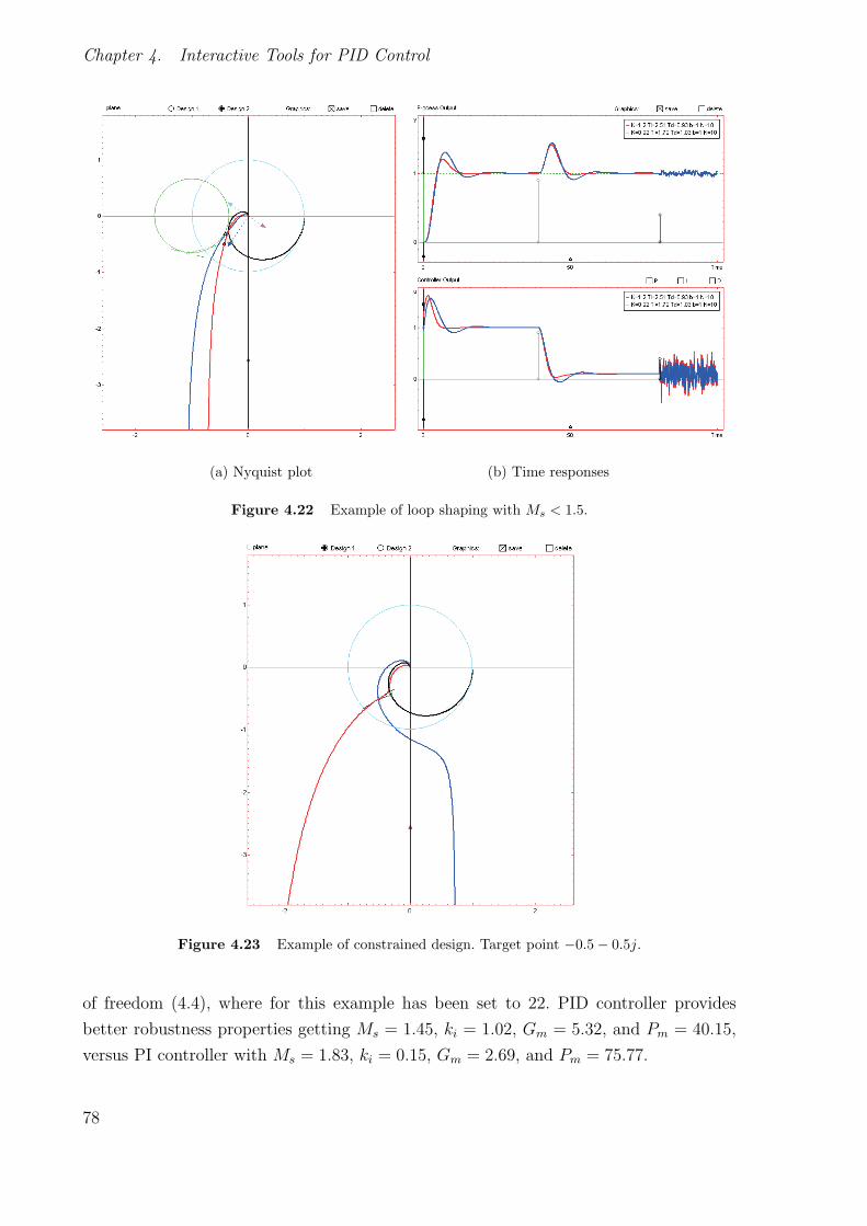
Chapter 4. Interactive Tools for PID Control
(a) Nyquist plot (b) Time responses
Figure 4.22 Example of loop shaping with Ms < 1.5.
Figure 4.23 Example of constrained design. Target point −0.5 − 0.5j.
of freedom (4.4), where for this example has been set to 22. PID controller provides
better robustness properties getting Ms = 1.45, ki = 1.02, Gm = 5.32, and Pm = 40.15,
versus PI controller with Ms = 1.83, ki = 0.15, Gm = 2.69, and Pm = 75.77.
78

4.2.2 Illustrative Examples
(a) Combined sensitivity constrained (b) Gain margin and sensitivity constrained
Figure 4.24 Example of constrained design. Sensitivity and gain margin constraints.
Similar examples to restrict the target point for phase margin, gain margin, or maxi-
mum values of the sensitivity functions can be performed, as represented in Figure 4.19.
Figure 4.24(a) shows an example where a combined sensitivity constraint is required for
Ms ≤ 2 and Mt ≤ 2. Such constraint is fulfilled in two different ways using a constrained
PID (in red) and a constrained PI (in blue). Another example combining sensitivity
function and gain margin constraints is shown in Figure 4.24(b), with the specification
that the gain margin is equal to 3 and Ms ≤ 2, maximizing the integral gain ki. So,
the constraint gain margin is chosen and the target point is located in such a way that
Gm = 3. Then, a constrained PID controller is selected, being the design point and the
slope modified until Ms ≤ 2 and the integral gain is maximized. The controller obtained
is given by k = 1.38, ki = 0.52, and kd = 0.54 for ω = 1.02 and slope = 32.
The derivative cliff
This example is available at the Settings menu of PID Loop Shaping [5]. The process
transfer function is the same that in previous examples (P (s) = 1/(s+ 1)4). It is desired
to maximize integral gain ki subject to the robustness constraint Ms ≤ 1.4. The obtained
controller provides the parameters k = 0.925, ki = 0.9, and kd = 2.86 where the Nyquist
plot of the loop transfer function is shown in red in Figure 4.25(a). It can be observed
that the Nyquist curve has a loop. This phenomenon is called derivative cliff (a deeper
79

Chapter 4. Interactive Tools for PID Control
(a) Nyquist plot (b) Time domain responses
Figure 4.25 Derivative cliff example
explanation can be found in [5]) and it is due to the fact that the obtained controller
has excessive phase lead, which is obtained by having PID controller with complex poles
(Ti < 4Td, in this example Ti = 0.33Td). Figure 4.25(b) shows, in red color, the time
response of this controller obtaining oscillatory outputs. For comparison issues, the results
for a controller with Ti = 4Td are shown in blue color in Figures 4.25(a) and (b) with the
controller parameters k = 1.1, ki = 0.36 and kd = 0.9. The responses for this controller
are better, even under larger overshoot in response to load disturbance.
Delayed system
Dead-times appear in many industrial processes, usually associated with mass or energy
transport, or due to the accumulation of a great number of low-order systems. Dead-
times produce an increase in the system phase lag, therefore decreasing the phase and
gain margins and limiting the response speed of the system (system bandwidth) [75],
[121].
An example is described in what follows in order to see the influence of the time
delay. The process transfer function is given by
80
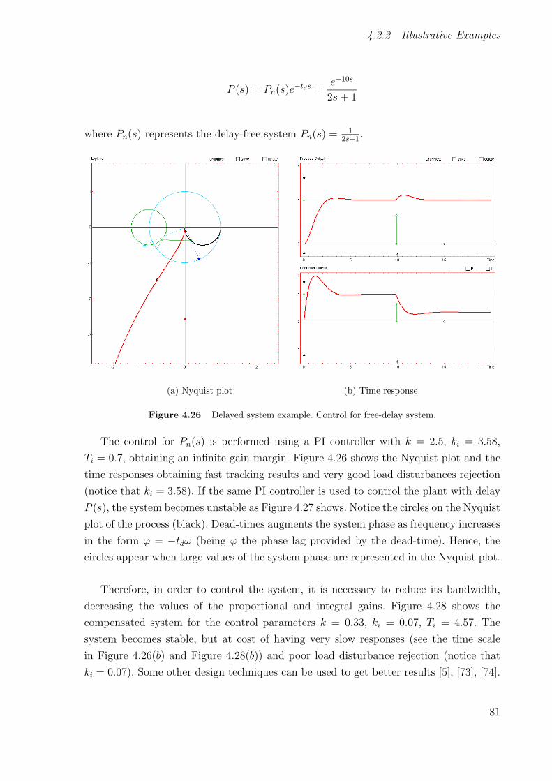
4.2.2 Illustrative Examples
P (s) = Pn(s)e−tds =
e−10s
2s+ 1
where Pn(s) represents the delay-free system Pn(s) = 12s+1
.
(a) Nyquist plot (b) Time response
Figure 4.26 Delayed system example. Control for free-delay system.
The control for Pn(s) is performed using a PI controller with k = 2.5, ki = 3.58,
Ti = 0.7, obtaining an infinite gain margin. Figure 4.26 shows the Nyquist plot and the
time responses obtaining fast tracking results and very good load disturbances rejection
(notice that ki = 3.58). If the same PI controller is used to control the plant with delay
P (s), the system becomes unstable as Figure 4.27 shows. Notice the circles on the Nyquist
plot of the process (black). Dead-times augments the system phase as frequency increases
in the form ϕ = −tdω (being ϕ the phase lag provided by the dead-time). Hence, the
circles appear when large values of the system phase are represented in the Nyquist plot.
Therefore, in order to control the system, it is necessary to reduce its bandwidth,
decreasing the values of the proportional and integral gains. Figure 4.28 shows the
compensated system for the control parameters k = 0.33, ki = 0.07, Ti = 4.57. The
system becomes stable, but at cost of having very slow responses (see the time scale
in Figure 4.26(b) and Figure 4.28(b)) and poor load disturbance rejection (notice that
ki = 0.07). Some other design techniques can be used to get better results [5], [73], [74].
81

Chapter 4. Interactive Tools for PID Control
(a) Nyquist plot (b) Time response
Figure 4.27 Delayed system example. Unstable results.
(a) Nyquist plot (b) Time response
Figure 4.28 Delayed system example. Stable system with bandwidth limitation.
82

4.3 PID Windup
4.3 PID Windup
Many aspects of PID control can be understood using linear models. There are, however,
some important nonlinear effects that are very common even in simple loops with PID
control. Integral windup can occur in loops where the process has saturations and the
controller has integral action. When the process saturates, the feedback loop is broken
and the integral may reach large values maintaining the control signal saturated for a
long time, resulting in large overshoots and undesirable transients [5].
The purpose of this module is to facilitate the understanding of integral windup and a
method for avoiding it (see [5]). There are many different ways to protect against windup.
Tracking is a simple method which was discussed in chapter 2 and is illustrated in the
block diagram in Figure 2.2. The module shows process outputs and control signals for
unlimited control signals, limited control signals without anti-windup, and limited control
signals with anti-windup (see Figure 4.29). Process models and controller parameters can
be selected in the same way as in the other modules. The saturation limits of the control
signal can be determined either by entering the values or by dragging the lines in the
saturation metaphor. The main aspects of the tool and some illustrative examples will
be shown in the following paragraphs.
4.3.1 Description of the Interactive Tool
This section briefly describes the main aspects of PID Windup. The main screen of the
tool is shown in Figure 4.29.
Process
It corresponds to the same Process zone that in previous tools. It provides the same
elements that in PID Basics, where a symbolic representation of the process transfer
function is available, and the process parameters can be modified by interactive sliders
or text edits (see Figure 4.29). The time delay is modified using an slider instead of a
text edit as in PID Basics or PID Loop Shaping. Then, the time delay effect on the
anti-windup mechanism can be easily analyzed.
Controller
This section contains the information about the controller parameters and actuator sat-
uration. Three kind of controllers with integral action can be selected (I, PI, PID), where
several sliders are available to modify the controller parameters including the tracking
time constant Tt used to reduce the integral effect. A saturation metaphor graphic is
83

Chapter 4. Interactive Tools for PID Control
Figure 4.29 The user interface of the module PID Windup, showing windup phenomenonand anti-windup technique.
also available in this zone. This graphic allows determining the saturation limits dragging
on the small red circle located on the upper saturation value (notice that a symmetric
saturation has been used; this choice has been selected for pedagogical purposes).
Graphics
Time responses for process output, control signal, and integral action are available in
three different graphics (Process Output, Controller Output, Integral term). In the same
way that in PID Basics, there exist multiple interactive graphical elements to modify:
set-point, load disturbance, measurement noise, and horizontal and vertical scales (see
Figure 4.29). These three graphics can simultaneously represent the controlled system in
linear mode, non-linear mode with windup phenomenon, and non-linear mode with anti-
windup technique. Such representations can be configured using the checkboxes located
on the top of Process Output graphic. There are three checkboxes called Linear, Windup,
and Antiwindup to include the associated signal in all graphics, that contain a legend for
84

4.3.1 Description of the Interactive Tool
the three signals, showing the linear mode in red, windup mode in blue, and antiwindup
one in green color. An example can be seen in Figure 4.30(a) where the three modes are
active.
A dotted pink vertical line which makes it easier to compare the time in the plots is
also available as Figure 4.30(a) shows. On the other hand, the saturation limits can be
modified using the dotted blue horizontal lines available in the Controller Output graphic
(see Figure 4.30).
(a) Several modes simultaneously (b) Proportional bands
Figure 4.30 Signal representation in PID Windup module.
The notion of proportional band is useful to understand the windup effect and is
included in PID Windup. The proportional band is defined as the range of process outputs
where the controller output is in the linear range [ymin, ymax]. For a PI controller, the
proportional band is limited by
ymin = bysp +I − umax
K
ymax = bysp +I − umin
K
where I is the integral term of a PI controller.
85

Chapter 4. Interactive Tools for PID Control
The same expressions hold for PID control if the proportional band is defined as the
band where the predicted output yp = y + Tddydt
is in the proportional band [ymin, ymax].
The proportional band has the width (umax − umin)/K and is centered at bysp + I/K −(umax + umin)/(2K).
On the top of figure Process Output there are two additional checkboxes called PB
Windup and PB Antiwindup. The activation of these options shows the proportional bands
for the windup and antwindup cases in the Process Output graphic. The proportional
bands are shown as dotted green and blue signals respectively, as Figure 4.30(b) shows.
Settings menu
The Settings menu is defined following the same structure that in previous modules. The
process transfer function can be chosen from the entry Process transfer functions, and
numerical values of the parameters can be introduced using the selection Controller pa-
rameters. Essential data and results can be saved and recalled using the Load/Save menu
options. The menu selection Simulation makes it possible to choose the simulation time,
and to activate the Sweep option which can be used to show the results for several values
of the tracking time constant (as will be seen later in an example). Several examples
from [5] can be loaded from the Examples entry.
4.3.2 Illustrative Examples
Some examples to explain integral windup are going to be described using PID Windup.
Understanding Windup Phenomenon
The windup phenomenon can be studied using the first entry from the Examples option
menu. This example has been extracted from [5] and uses a pure integrator process
P (s) = 1s
controlled by a PI controller with K = 1, Ti = 1.2, b = 1 with the control
signal limited to ±0.1. Figure 4.31(a) shows the time responses for this example. The
control signal is saturated from the first time instant. The process output and the integral
term are increasing while the control error is positive. Once the process output exceeds
the set-point, the control error turns to be negative, but the control signal remains
saturated due to the large value of the integral term (windup phenomenon). Looking
at the dotted pink vertical line in Figure 4.31(a), the integral term reaches its largest
value at t = 10, when the error goes through zero. So, the control signal does not leave
the saturation limit until the error has been negative for a sufficiently long time to let
the integral part come down to a small level. An interesting aspect can be observed in
86
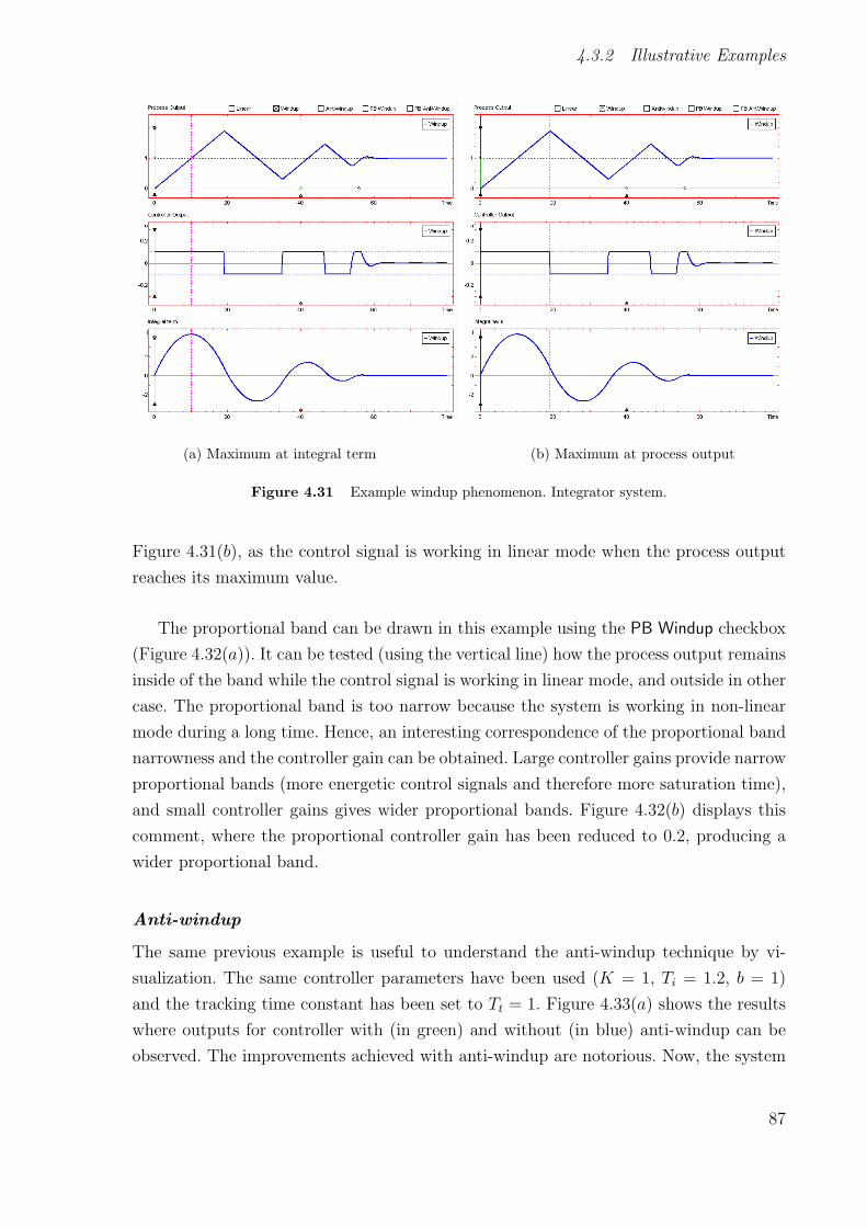
4.3.2 Illustrative Examples
(a) Maximum at integral term (b) Maximum at process output
Figure 4.31 Example windup phenomenon. Integrator system.
Figure 4.31(b), as the control signal is working in linear mode when the process output
reaches its maximum value.
The proportional band can be drawn in this example using the PB Windup checkbox
(Figure 4.32(a)). It can be tested (using the vertical line) how the process output remains
inside of the band while the control signal is working in linear mode, and outside in other
case. The proportional band is too narrow because the system is working in non-linear
mode during a long time. Hence, an interesting correspondence of the proportional band
narrowness and the controller gain can be obtained. Large controller gains provide narrow
proportional bands (more energetic control signals and therefore more saturation time),
and small controller gains gives wider proportional bands. Figure 4.32(b) displays this
comment, where the proportional controller gain has been reduced to 0.2, producing a
wider proportional band.
Anti-windup
The same previous example is useful to understand the anti-windup technique by vi-
sualization. The same controller parameters have been used (K = 1, Ti = 1.2, b = 1)
and the tracking time constant has been set to Tt = 1. Figure 4.33(a) shows the results
where outputs for controller with (in green) and without (in blue) anti-windup can be
observed. The improvements achieved with anti-windup are notorious. Now, the system
87

Chapter 4. Interactive Tools for PID Control
(a) Proportional band K = 1 (b) Proportional band K = 0.4
Figure 4.32 Example windup phenomenon. Proportional band.
(a) Anti-windup (b) Effect of Tt
Figure 4.33 Example anti-windup technique. Tt effect.
only remains in saturation for a short time period, being the output of the integral term
considerably reduced. The proportional band for PI controller with anti-windup is shown
in the same figure. It can be observed how a wider proportional band than for PI without
anti-windup (Figure 4.33(a)) is obtained, remaining the process output inside of it most
88
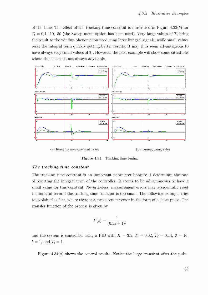
4.3.2 Illustrative Examples
of the time. The effect of the tracking time constant is illustrated in Figure 4.33(b) for
Tt = 0.1, 10, 50 (the Sweep menu option has been used). Very large values of Tt bring
the result to the windup phenomenon producing large integral signals, while small values
reset the integral term quickly getting better results. It may thus seem advantageous to
have always very small values of Tt. However, the next example will show some situations
where this choice is not always advisable.
(a) Reset by measurement noise (b) Tuning using rules
Figure 4.34 Tracking time tuning.
The tracking time constant
The tracking time constant is an important parameter because it determines the rate
of resetting the integral term of the controller. It seems to be advantageous to have a
small value for this constant. Nevertheless, measurement errors may accidentally reset
the integral term if the tracking time constant is too small. The following example tries
to explain this fact, where there is a measurement error in the form of a short pulse. The
transfer function of the process is given by
P (s) =1
(0.5s+ 1)2
and the system is controlled using a PID with K = 3.5, Ti = 0.52, Td = 0.14, ℵ = 10,
b = 1, and Tt = 1.
Figure 4.34(a) shows the control results. Notice the large transient after the pulse.
89

Chapter 4. Interactive Tools for PID Control
The integral term is excessively reduced, even reaching negative values. Some simple
rules that have been suggested for the tracking time, Tt =√TiTd and Tt = (Ti + Td)/2
[5], can be used to tune Tt and avoid these problems. Figure 4.34(b) shows an example
with Tt = (Ti + Td)/2 = 0.33 where the response has been considerably improved.
90

5
Interactive Tools for GPC
Control systems have traditionally been designed using an iterative process of synthe-
sis and analysis until specifications are accomplished, GPC being an exponent of this
iterative procedure. The goal of this chapter is to merge the two phases in such a way
that modifying a system parameter produces an immediate effect. In this way, design-
ing becomes dynamic, and the student perceives a change in the performance crite-
ria. This chapter presents two IT developed for learning GPC: SISO-GPCIT (Gener-
alized Predictive Control Interactive Tool for Single-Input Single-Output Systems)[58]
and MIMO-GPCIT (Generalized Predictive Control Interactive Tool for Multiple-Input
Multiple-Output Systems)[56]. These tools have been developed to help students learn
and understand the basic and advanced concepts involved in GPC, and to provide them
with a strong theoretical base and engineering skills, which is a major challenge in Au-
tomatic Control education [94]. These tools have been developed using the interactive
design CAD tool Sysquake, developed n the Institute of Automatics of the Federal Poly-
technic School of Lausanne (Switzerland) [125].
5.1 SISO-GPCIT
SISO-GPCIT is an IT which helps to demystify abstract mathematical concepts involved
in GPC through visualization by using especially chosen examples, while enhancing stu-
dent skills, motivation, and the ability to understand and solve control problems [41].
By using SISO-GPCIT, students can put into practice their knowledge of GPC. Stu-
dents can study the effect of tuning knobs and constraints in the design and perfor-
mance of the controller, while analyzing disturbance rejection, robustness, and stabil-
ity. Several examples selected from typical MPC textbooks are included in the tool.
SISO-GPCIT is freeware [57], can run under a Windows-type operating system, and re-
quires no programming to create examples; indeed, only dialog box and mouse operations
91

Chapter 5. Interactive Tools for GPC
are necessary. The effort is focused on understanding the fundamental concepts of the
technique without writing code, allowing the user to interactively analyze the effect of
plant/model/controller parameter modifications on the performance and stability of the
closed-loop system.
SISO-GPCIT uses a transfer function system model [28]. The author believes this type
of formulation, based entirely on measurable input-output information, and in which es-
sential elements (poles and zeros) have a physical meaning, is more intuitive for the
student. This approach is fundamental for designing IT, in which different system rep-
resentations are simultaneously modified and updated. State-space system descriptions
often use canonical representations in which the physical meaning is lost, increasing the
complexity of system representation when working with IT. In our experience, it is easier
for students to understand the basics of MPC techniques by using transfer-function-based
system descriptions. Once they understand the core aspects, students can face more com-
plex MPC techniques.
5.1.1 Description of the interactive tool
This section briefly describes SISO-GPCIT, and how it can be used [57]. The main screen
of the tool is shown in Figure 5.1
Continuous-time poles and zeros
The s-plane poles (x) and zeros (o) of the linear system (in green), and its model (in
orange) are shown in Figure 5.1. The same color scheme is applied to the closed-loop
step responses. T-polynomial roots are in black (). The location of poles and zeros can
be interactively modified by drag-and-drop at these points, and it is possible to define
transfer functions with a dialog box of the Settings menu, as well as add or delete poles,
zeros, and integrators over the plot using Operations over poles/zeros.
Discrete-time poles and zeros
The z-plane poles and zeros, obtained from discretizing the continuous transfer functions,
are represented using the same colors and symbols like those of the s-plane poles and
zeros. Changes performed in the s-plane chart are automatically updated in the z-plane
chart. The closed-loop system poles (in blue) allow closed-loop stability to be studied.
Several discretization methods are available in the Settings menu.
92
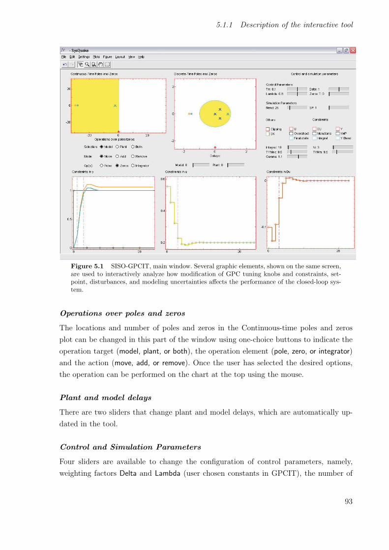
5.1.1 Description of the interactive tool
Figure 5.1 SISO-GPCIT, main window. Several graphic elements, shown on the same screen,are used to interactively analyze how modification of GPC tuning knobs and constraints, set-point, disturbances, and modeling uncertainties affects the performance of the closed-loop sys-tem.
Operations over poles and zeros
The locations and number of poles and zeros in the Continuous-time poles and zeros
plot can be changed in this part of the window using one-choice buttons to indicate the
operation target (model, plant, or both), the operation element (pole, zero, or integrator)
and the action (move, add, or remove). Once the user has selected the desired options,
the operation can be performed on the chart at the top using the mouse.
Plant and model delays
There are two sliders that change plant and model delays, which are automatically up-
dated in the tool.
Control and Simulation Parameters
Four sliders are available to change the configuration of control parameters, namely,
weighting factors Delta and Lambda (user chosen constants in GPCIT), the number of
93

Chapter 5. Interactive Tools for GPC
zeros in the T-polynomial (Zeros T), and sampling time (Tm). Two other sliders enable
the user to modify the simulation parameters, end time (Nend), and the number of set-
point steps (SP).
Other parameters
This part of the window contains two boxes, one for Clipping (saturating) the control
signal obtained by unconstrained GPC, which is used in some industrial controls, and
the other for activating a random noise disturbance, whose amplitude and start time can
be modified in the Constraints in Y plot.
(a) Envelope, and final state constraints. (b) Step, impulse, and noise disturbances.
Figure 5.2 Closed-loop response output signals. The system output is affected by changesin the set-point, constraints, and disturbances. These graphics show how the user can add andmodify these changes.
GPC constraints
Several active boxes allow the user to select the types of constraints (included in Table
2.3), which can be configured by moving the active points in the envelope constraints
(plots at bottom) using the mouse. The effect is automatically updated in the other
charts.
Closed-loop response and output constraints
Figure 5.2(a) shows the closed-loop system response with a pre-programmed set-point
in GPC. The number of step changes in the set-point can be modified by using the SP
slider in Control and Simulation Parameters. The amplitude and shape of the set-point
(in violet) can be interactively changed by clicking on the active points, which are small
circles identified by colors. When two or more points collapse into a single point, the
resulting color corresponds to the point that can still be moved. Prediction horizons N1
and N2 are represented in this plot as vertical discontinuous blue lines. These parameters,
as well as the output amplitude constraints, represented by two horizontal discontinuous
94
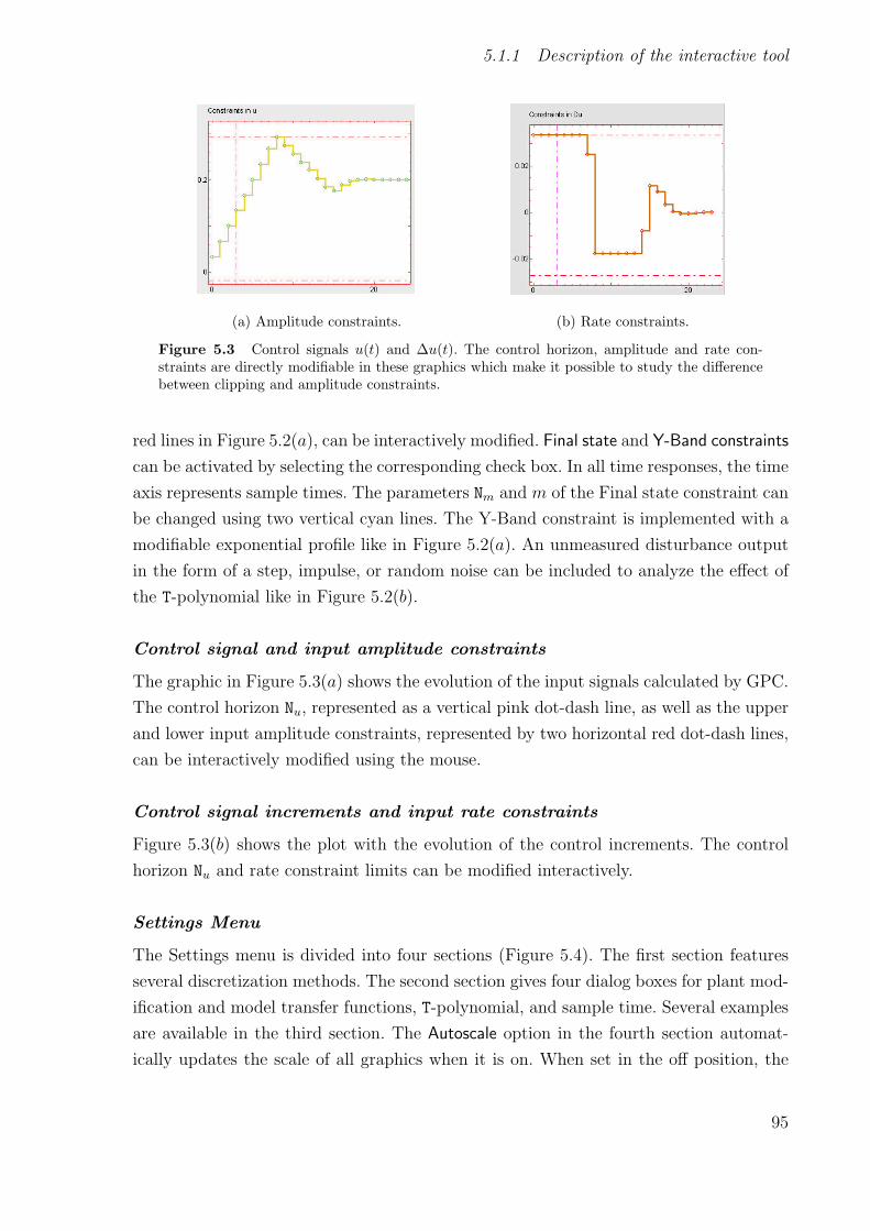
5.1.1 Description of the interactive tool
(a) Amplitude constraints. (b) Rate constraints.
Figure 5.3 Control signals u(t) and ∆u(t). The control horizon, amplitude and rate con-straints are directly modifiable in these graphics which make it possible to study the differencebetween clipping and amplitude constraints.
red lines in Figure 5.2(a), can be interactively modified. Final state and Y-Band constraints
can be activated by selecting the corresponding check box. In all time responses, the time
axis represents sample times. The parameters Nm and m of the Final state constraint can
be changed using two vertical cyan lines. The Y-Band constraint is implemented with a
modifiable exponential profile like in Figure 5.2(a). An unmeasured disturbance output
in the form of a step, impulse, or random noise can be included to analyze the effect of
the T-polynomial like in Figure 5.2(b).
Control signal and input amplitude constraints
The graphic in Figure 5.3(a) shows the evolution of the input signals calculated by GPC.
The control horizon Nu, represented as a vertical pink dot-dash line, as well as the upper
and lower input amplitude constraints, represented by two horizontal red dot-dash lines,
can be interactively modified using the mouse.
Control signal increments and input rate constraints
Figure 5.3(b) shows the plot with the evolution of the control increments. The control
horizon Nu and rate constraint limits can be modified interactively.
Settings Menu
The Settings menu is divided into four sections (Figure 5.4). The first section features
several discretization methods. The second section gives four dialog boxes for plant mod-
ification and model transfer functions, T-polynomial, and sample time. Several examples
are available in the third section. The Autoscale option in the fourth section automat-
ically updates the scale of all graphics when it is on. When set in the off position, the
95
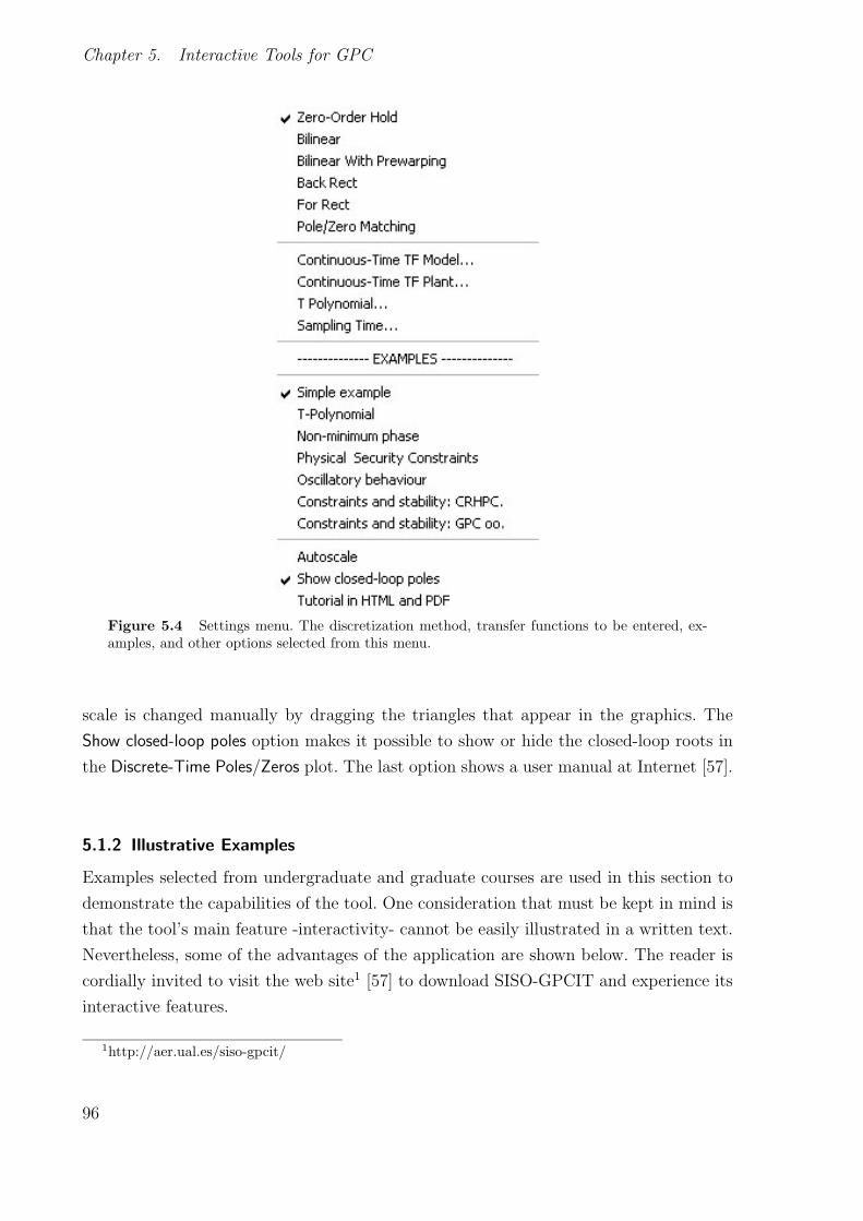
Chapter 5. Interactive Tools for GPC
Figure 5.4 Settings menu. The discretization method, transfer functions to be entered, ex-amples, and other options selected from this menu.
scale is changed manually by dragging the triangles that appear in the graphics. The
Show closed-loop poles option makes it possible to show or hide the closed-loop roots in
the Discrete-Time Poles/Zeros plot. The last option shows a user manual at Internet [57].
5.1.2 Illustrative Examples
Examples selected from undergraduate and graduate courses are used in this section to
demonstrate the capabilities of the tool. One consideration that must be kept in mind is
that the tool’s main feature -interactivity- cannot be easily illustrated in a written text.
Nevertheless, some of the advantages of the application are shown below. The reader is
cordially invited to visit the web site1 [57] to download SISO-GPCIT and experience its
interactive features.
1http://aer.ual.es/siso-gpcit/
96
5.1.2 Illustrative Examples
Unconstrained case
The first example is taken from [26], in which an unconstrained GPC controller is de-
signed for a plant described by
(1 − 0.8z−1)y(t) = (0.4 + 0.6z−1)u(t− 1) +ε(t)
(1 − z−1)
With the help of the interactive features, students can select the most appropriate
parameters for their application and control specifications. For this example an explicit
solution given by ∆u = −H−1b can be found for the unconstrained linear case, which is
used by GPCIT instead of solving a quadratic programming problem. Figure 5.5 shows
the results of different tuning knob values.
Effect of the T-polynomial
As shown in [26], [133], the T-polynomial can be used to improve GPC robustness and
disturbance response. The plant
(1 − 0.9z−1)y(t) = (0.1z−1 + 0.2z−2)u(t),
included in [29] as an illustrative example, is used here. Figure 5.6(a) shows the closed-
loop response with (N1,N2,Nu, δ, λ) =(1,10,1,1,0) and no disturbances. Figures 5.6(b) and
(c) show the results of applying a GPC controller with the same tuning knobs and with
T(z−1) = 1 and T(z−1) = (1 − 0.8z−1), respectively. This example, which illustrates
the effect of disturbances, consists of an initial step in the set-point, followed by an
additional load-disturbance step acting on the output along with a period of uncorrelated
random noise, such as measurement noise added to the plant output. Note that the step
responses of the controllers in the figure are the same. For T = 1 the load disturbance
is rapidly eliminated, but the output noise induces a high variance control signal and
output fluctuations, while for T = 1 − 0.8z−1 the controller takes longer to eliminate
the load disturbance, although the response to output noise is better in the sense that
control variance is reduced.
97
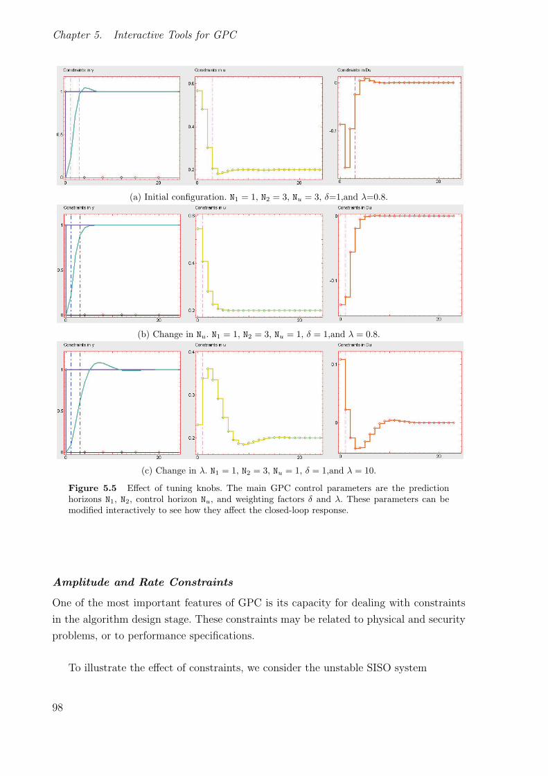
Chapter 5. Interactive Tools for GPC
(a) Initial configuration. N1 = 1, N2 = 3, Nu = 3, δ=1,and λ=0.8.
(b) Change in Nu. N1 = 1, N2 = 3, Nu = 1, δ = 1,and λ = 0.8.
(c) Change in λ. N1 = 1, N2 = 3, Nu = 1, δ = 1,and λ = 10.
Figure 5.5 Effect of tuning knobs. The main GPC control parameters are the predictionhorizons N1, N2, control horizon Nu, and weighting factors δ and λ. These parameters can bemodified interactively to see how they affect the closed-loop response.
Amplitude and Rate Constraints
One of the most important features of GPC is its capacity for dealing with constraints
in the algorithm design stage. These constraints may be related to physical and security
problems, or to performance specifications.
To illustrate the effect of constraints, we consider the unstable SISO system
98
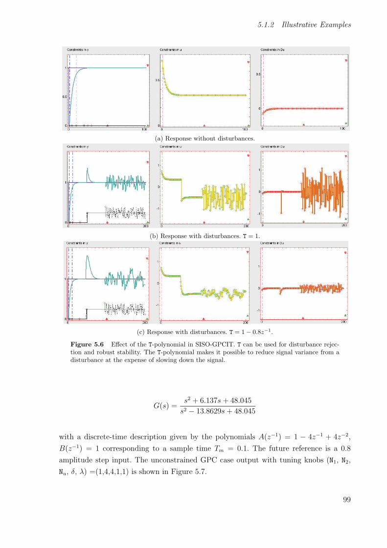
5.1.2 Illustrative Examples
(a) Response without disturbances.
(b) Response with disturbances. T = 1.
(c) Response with disturbances. T = 1 − 0.8z−1.
Figure 5.6 Effect of the T-polynomial in SISO-GPCIT. T can be used for disturbance rejec-tion and robust stability. The T-polynomial makes it possible to reduce signal variance from adisturbance at the expense of slowing down the signal.
G(s) =s2 + 6.137s+ 48.045
s2 − 13.8629s+ 48.045
with a discrete-time description given by the polynomials A(z−1) = 1 − 4z−1 + 4z−2,
B(z−1) = 1 corresponding to a sample time Tm = 0.1. The future reference is a 0.8
amplitude step input. The unconstrained GPC case output with tuning knobs (N1, N2,
Nu, δ, λ) =(1,4,4,1,1) is shown in Figure 5.7.
99
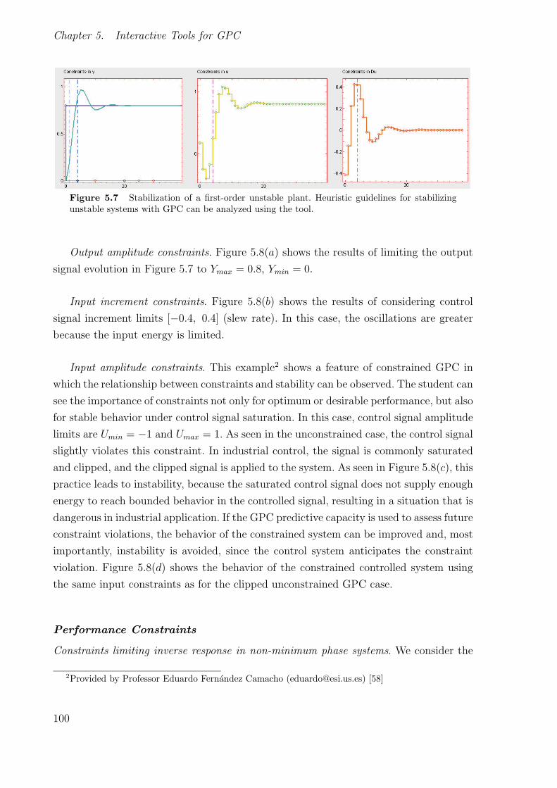
Chapter 5. Interactive Tools for GPC
Figure 5.7 Stabilization of a first-order unstable plant. Heuristic guidelines for stabilizingunstable systems with GPC can be analyzed using the tool.
Output amplitude constraints. Figure 5.8(a) shows the results of limiting the output
signal evolution in Figure 5.7 to Ymax = 0.8, Ymin = 0.
Input increment constraints. Figure 5.8(b) shows the results of considering control
signal increment limits [−0.4, 0.4] (slew rate). In this case, the oscillations are greater
because the input energy is limited.
Input amplitude constraints. This example2 shows a feature of constrained GPC in
which the relationship between constraints and stability can be observed. The student can
see the importance of constraints not only for optimum or desirable performance, but also
for stable behavior under control signal saturation. In this case, control signal amplitude
limits are Umin = −1 and Umax = 1. As seen in the unconstrained case, the control signal
slightly violates this constraint. In industrial control, the signal is commonly saturated
and clipped, and the clipped signal is applied to the system. As seen in Figure 5.8(c), this
practice leads to instability, because the saturated control signal does not supply enough
energy to reach bounded behavior in the controlled signal, resulting in a situation that is
dangerous in industrial application. If the GPC predictive capacity is used to assess future
constraint violations, the behavior of the constrained system can be improved and, most
importantly, instability is avoided, since the control system anticipates the constraint
violation. Figure 5.8(d) shows the behavior of the constrained controlled system using
the same input constraints as for the clipped unconstrained GPC case.
Performance Constraints
Constraints limiting inverse response in non-minimum phase systems. We consider the
2Provided by Professor Eduardo Fernandez Camacho ([email protected]) [58]
100

5.1.2 Illustrative Examples
(a) Output constraints.
(b) Constraints on control increments.
(c) Unconstrained case with clipped control signal.
(d) Constraints on control signal amplitude.
Figure 5.8 Physical and security constraints. Most actuators are limited by constraints suchas amplitude and rate, and the system output must usually lie between two values. Theseconstraints are inherent in the GPC design process, and can be switched on by drag-and-drop.
101

Chapter 5. Interactive Tools for GPC
(a) Non-minimum phase plant and corresponding inverse response.
(b) NMP constraint active limiting the inverse response.
Figure 5.9 Non-minimum phase system. By selecting the NMP constraint, the inverse re-sponse can be limited in NMP systems. With GPC performance constraints, the amplitude ofthe inverse response can be limited.
system
G(s) =1 − s
s+ 1,
discussed in [2]. Figure 5.9(a) shows the response with (N1, N2, Nu, δ, λ)=(1,30,10,1,0.1),
where the inverse response typical of non-minimum phase behavior can be observed.
If the NMP active box in the Constraints parameters is set, the non-minimum phase
behavior can be limited (Figure 5.9(b)). This situation is relevant to industrial plants in-
volving interaction between control loops. Note that the theoretical non-minimum phase
constraint in Table 2.3 has to be applied with a threshold to avoid feasibility problems.
Monotone behavior constraint. We consider the oscillatory system
G(s) =50
s2 + 25
taken from [26] and [102]. The system, sampled at 0.1, shows oscillation before reaching
102

5.1.2 Illustrative Examples
the set-point, as shown in Figure 5.10(a), with (N1, N2, Nu, δ, λ)=(1, 11, 11, 1, 50).
Monotone behavior constraints can be applied to avoid this type of response. The results
obtained for the same tuning knobs selected above are shown in Figure 5.10(b). The
oscillations have practically disappeared. Note that the prediction and control horizons
used are quite large. This behavior is due to cancellation of the oscillatory mode in the
open loop system, and a large control horizon will have to be considered to obtain a
feasible solution.
(a) Oscillatory behavior.
(b) Monotone constraint active.
Figure 5.10 Monotone behavior constraint. In many systems, oscillation occurs before theset-point is reached. Such behavior may not be desirable, especially when one system is connectedto another. This graph shows how this behavior can be limited.
Envelope constraints. Sometimes system output values must follow a trajectory within
an envelope. An example is presented in Figure 5.11, where this type of requirement has
been introduced in the control system studied in Figure 5.10 by forcing the output of
the system to be included in the envelope formed by two curves with exponential shape.
Constraints and stability
Many techniques relating MPC constraints and stability can be found in the literature
[107], [26]. One well-known technique is Constrained Receding Horizon Predictive Control
103
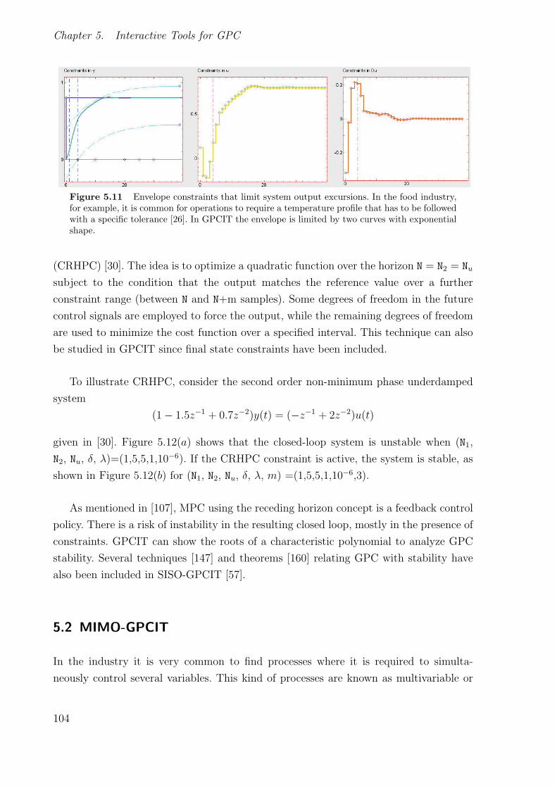
Chapter 5. Interactive Tools for GPC
Figure 5.11 Envelope constraints that limit system output excursions. In the food industry,for example, it is common for operations to require a temperature profile that has to be followedwith a specific tolerance [26]. In GPCIT the envelope is limited by two curves with exponentialshape.
(CRHPC) [30]. The idea is to optimize a quadratic function over the horizon N = N2 = Nu
subject to the condition that the output matches the reference value over a further
constraint range (between N and N+m samples). Some degrees of freedom in the future
control signals are employed to force the output, while the remaining degrees of freedom
are used to minimize the cost function over a specified interval. This technique can also
be studied in GPCIT since final state constraints have been included.
To illustrate CRHPC, consider the second order non-minimum phase underdamped
system
(1 − 1.5z−1 + 0.7z−2)y(t) = (−z−1 + 2z−2)u(t)
given in [30]. Figure 5.12(a) shows that the closed-loop system is unstable when (N1,
N2, Nu, δ, λ)=(1,5,5,1,10−6). If the CRHPC constraint is active, the system is stable, as
shown in Figure 5.12(b) for (N1, N2, Nu, δ, λ, m) =(1,5,5,1,10−6,3).
As mentioned in [107], MPC using the receding horizon concept is a feedback control
policy. There is a risk of instability in the resulting closed loop, mostly in the presence of
constraints. GPCIT can show the roots of a characteristic polynomial to analyze GPC
stability. Several techniques [147] and theorems [160] relating GPC with stability have
also been included in SISO-GPCIT [57].
5.2 MIMO-GPCIT
In the industry it is very common to find processes where it is required to simulta-
neously control several variables. This kind of processes are known as multivariable or
104
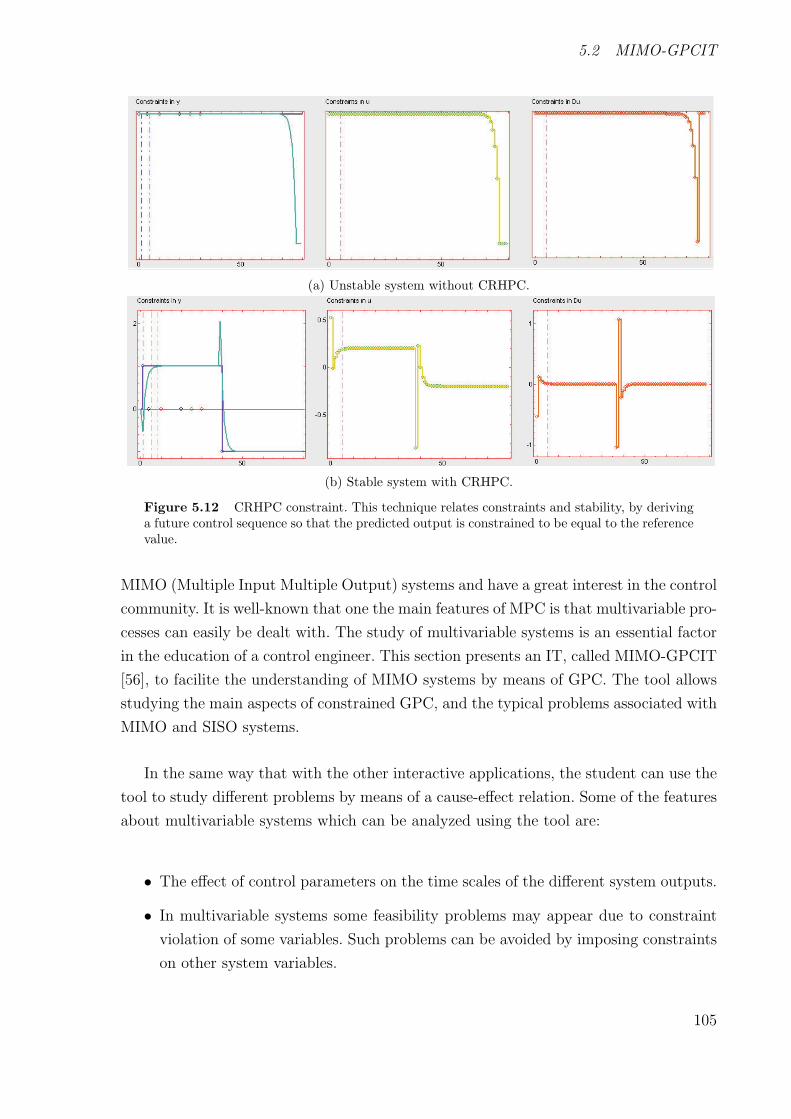
5.2 MIMO-GPCIT
(a) Unstable system without CRHPC.
(b) Stable system with CRHPC.
Figure 5.12 CRHPC constraint. This technique relates constraints and stability, by derivinga future control sequence so that the predicted output is constrained to be equal to the referencevalue.
MIMO (Multiple Input Multiple Output) systems and have a great interest in the control
community. It is well-known that one the main features of MPC is that multivariable pro-
cesses can easily be dealt with. The study of multivariable systems is an essential factor
in the education of a control engineer. This section presents an IT, called MIMO-GPCIT
[56], to facilite the understanding of MIMO systems by means of GPC. The tool allows
studying the main aspects of constrained GPC, and the typical problems associated with
MIMO and SISO systems.
In the same way that with the other interactive applications, the student can use the
tool to study different problems by means of a cause-effect relation. Some of the features
about multivariable systems which can be analyzed using the tool are:
• The effect of control parameters on the time scales of the different system outputs.
• In multivariable systems some feasibility problems may appear due to constraint
violation of some variables. Such problems can be avoided by imposing constraints
on other system variables.
105
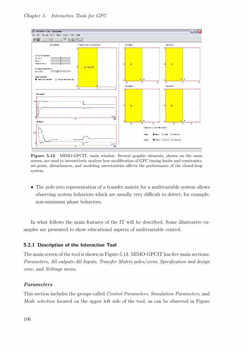
Chapter 5. Interactive Tools for GPC
Figure 5.13 MIMO-GPCIT, main window. Several graphic elements, shown on the samescreen, are used to interactively analyze how modification of GPC tuning knobs and constraints,set-point, disturbances, and modeling uncertainties affects the performance of the closed-loopsystem.
• The pole-zero representation of a transfer matrix for a multivariable system allows
observing system behaviors which are usually very difficult to detect; for example,
non-minimum phase behaviors.
In what follows the main features of the IT will be described. Some illustrative ex-
amples are presented to show educational aspects of multivariable control.
5.2.1 Description of the Interactive Tool
The main screen of the tool is shown in Figure 5.13. MIMO-GPCIT has five main sections:
Parameters, All outputs-All Inputs, Transfer Matrix poles/zeros, Specification and design
zone, and Settings menu.
Parameters
This section includes the groups called Control Parameters, Simulation Parameters, and
Mode selection located on the upper left side of the tool, as can be observed in Figure
106

5.2.1 Description of the Interactive Tool
5.13. Using the first group, the user can modify the sample time (Tm) and the weighting
factors Delta and Lambda (which have been considered as constants in the application).
The second group allows modifying the simulation time (Nend), and from the third group
the user can choose the desired working mode, Plant specification mode or Design and
Analysis mode. Depending on the selected mode, the right side of the tool will change
in order to show the user the appropriate options.
All outputs-All Inputs
This zone is placed below the previous one (as Figure 5.13 shows) and is divided into two
parts. The first one (All-outputs) shows the closed-loop evolution for all system outputs
with the associated set-points. Each output and its reference are represented in the same
color. The second part (All-inputs) shows closed-loop evolution for the system inputs. The
aim of this area is to permit the user visualizing permanently and simultaneously the
evolution of the system outputs and inputs. So, the user can observe the effect of some
parameters over all the system variables, and how the different variables can influence
each others.
Figure 5.14 Design and analysis zone.
107
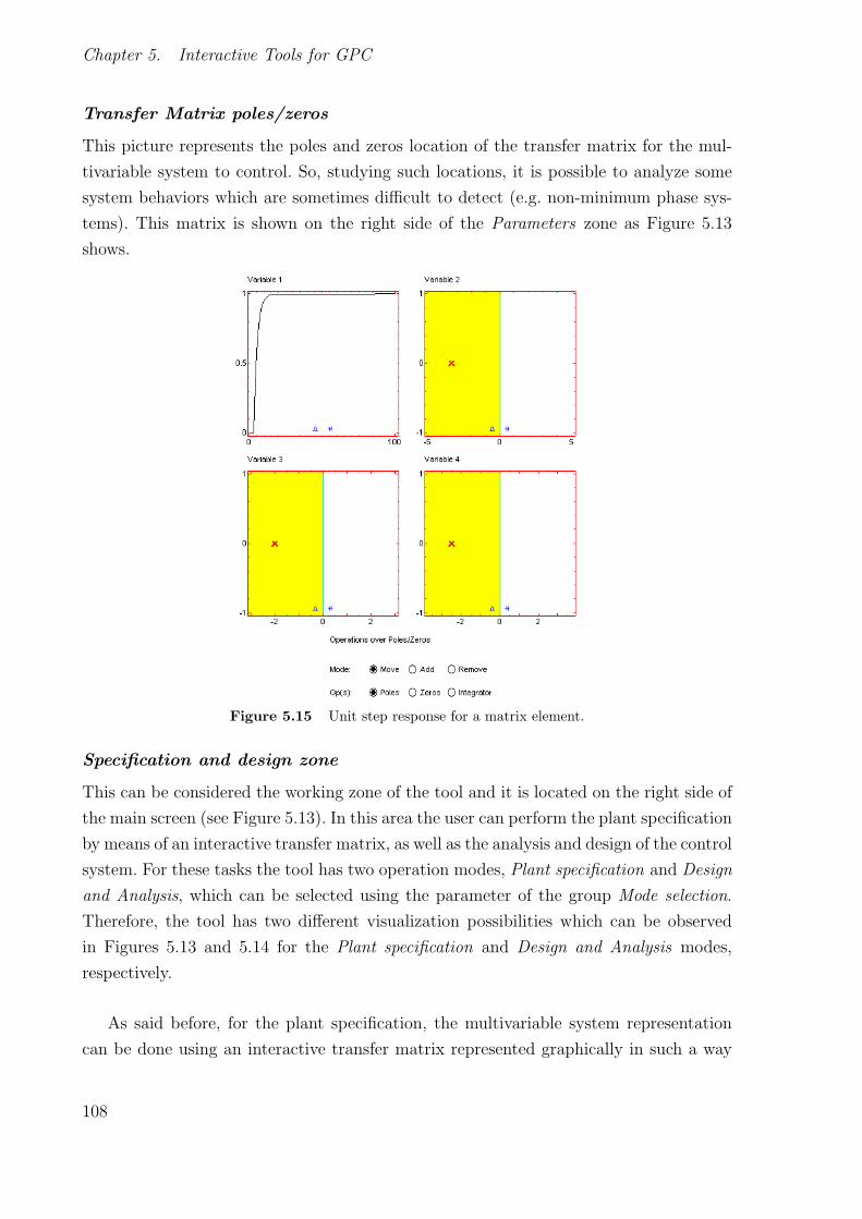
Chapter 5. Interactive Tools for GPC
Transfer Matrix poles/zeros
This picture represents the poles and zeros location of the transfer matrix for the mul-
tivariable system to control. So, studying such locations, it is possible to analyze some
system behaviors which are sometimes difficult to detect (e.g. non-minimum phase sys-
tems). This matrix is shown on the right side of the Parameters zone as Figure 5.13
shows.
Figure 5.15 Unit step response for a matrix element.
Specification and design zone
This can be considered the working zone of the tool and it is located on the right side of
the main screen (see Figure 5.13). In this area the user can perform the plant specification
by means of an interactive transfer matrix, as well as the analysis and design of the control
system. For these tasks the tool has two operation modes, Plant specification and Design
and Analysis, which can be selected using the parameter of the group Mode selection.
Therefore, the tool has two different visualization possibilities which can be observed
in Figures 5.13 and 5.14 for the Plant specification and Design and Analysis modes,
respectively.
As said before, for the plant specification, the multivariable system representation
can be done using an interactive transfer matrix represented graphically in such a way
108

5.2.1 Description of the Interactive Tool
Figure 5.16 Zoom over poles/zeros.
that, each matrix element contains the s-plane pole-zero location (x for poles and o
for zeros) of the transfer function associated to some system output with respect some
system input. The matrix elements are interactive graphics in which the user can define
each transfer function adding/moving/deleting poles and zeros. The different options to
work interactively on each matrix element are shown below the transfer matrix. In order
to modify the poles/zeros location, the user must select the associated option (Move and
Poles, or Zeros), put the mouse on the pole or zero to modify and, keeping pressed the left
button, move the pole or zero to the desired location. In the case of adding or removing
a pole/zero, the user must choose the correct options (Add or Remove, and Poles or
Zeros), and click once in the desired location (for the Add case) or in the pole/zero to
remove (for the Remove case). Each matrix element has a couple of small icons in the
middle of the horizontal axis. The one with triangle shape allows visualizing the unit
step response (see Figure 5.15) for the associated matrix element. The another one with
star shape allows widening (zoom) the matrix element (see Figure 5.16). After selecting
one of these options, the user must choose the same option again in order to return at
the previous screen.
Once the plant has been specified, the control parameters can be set, including the
109
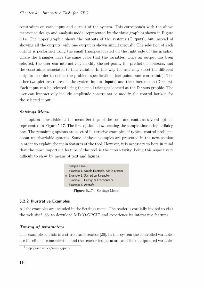
Chapter 5. Interactive Tools for GPC
constraints on each input and output of the system. This corresponds with the above
mentioned design and analysis mode, represented by the three graphics shown in Figure
5.14. The upper graphic shows the outputs of the systems (Outputs), but instead of
showing all the outputs, only one output is shown simultaneously. The selection of each
output is performed using the small triangles located on the right side of this graphic,
where the triangles have the same color that the variables. Once an output has been
selected, the user can interactively modify the set-point, the prediction horizons, and
the constraints associated to that variable. In this way the user may select the different
outputs in order to define the problem specifications (set-points and constraints). The
other two pictures represent the system inputs (Inputs) and their increments (Dinputs).
Each input can be selected using the small triangles located at the Dinputs graphic. The
user can interactively include amplitude constraints or modify the control horizon for
the selected input.
Settings Menu
This option is available at the menu Settings of the tool, and contains several options
represented in Figure 5.17. The first option allows setting the sample time using a dialog
box. The remaining options are a set of illustrative examples of typical control problems
about multivariable systems. Some of these examples are presented in the next section
in order to explain the main features of the tool. However, it is necessary to bore in mind
that the most important feature of the tool is the interactivity, being this aspect very
difficult to show by means of text and figures.
Figure 5.17 Settings Menu.
5.2.2 Illustrative Examples
All the examples are included in the Settings menu. The reader is cordially invited to visit
the web site3 [56] to download MIMO-GPCIT and experience its interactive features.
Tuning of parameters
This example consists in a stirred tank reactor [26]. In this system the controlled variables
are the effluent concentration and the reactor temperature, and the manipulated variables
3http://aer.ual.es/mimo-gpcit/
110

5.2.2 Illustrative Examples
are the feed flow rate and the flow of coolant in the jacket. The transfer function matrix
for this TITO (Two Inputs Two Outputs) system is given by
⎡⎣ Y1(s)
Y2(s)
⎤⎦ =
⎡⎣ 1
1+0.1s5
1+s
11+0.5s
21+0.4s
⎤⎦⎡⎣ U1(s)
U2(s)
⎤⎦
Figure 5.18 Stirred tank reactor.
(a) Modification of N2 from 3 to 9 for the output Y2. (b) Modification of λ from 0.05 to 0.001.
Figure 5.19 Examples of tuning.
Figure 5.18 shows the closed-loop response using MIMO-GPCIT. The prediction hori-
zons have been set to 3 for both output variables, the control horizons to 2 also for both
111

Chapter 5. Interactive Tools for GPC
input variables, and the weighting factors δ and λ to 1 and 0.1, respectively. The set-
points are 0.5 for the effluent concentration and 0.3 for the reactor temperature. At in-
stant time 60, the effluent concentration reference is modified from 0.5 to 0.4, influencing
all system variables, mainly the reactor temperature. In the same way the other control
parameters (control and prediction horizons, weighting factors, ...) can be modified to
observe their influence on the system variables. Figure 5.19(a) shows the modification
of the prediction horizon for the reactor temperature from 3 to 9 sample periods. Such
modification produces the overshoot reduction of this variable, at expense of a slower
response of the reactor temperature. Thus, the interrelation between variables can be
analyzed in this example.
In order to study the effect of the weighting factors, the λ factor has been changed
from 0.05 (see Figure 5.18) to 0.001 (Figure 5.19(b)). As can be seen the output variables
reach their respective references faster but with large control effort.
Including constraints
As said in previous chapters, constraints are usually related with physical or security
limitations, and performance criteria. Predictive control algorithms have the ability of
anticipating to the constraints violation, so avoiding deterioration in the system behavior.
A couple of examples are presented in order to show the constraint treatment using
MIMO-GPCIT.
Distillation column: this system [26] has three inputs and three outputs, where the
manipulated variables are the top draw rate, the side draw rate, and the bottom reflux
duty; and the controlled variables are the top and side product compositions, and the
bottom temperature. Figure 5.20 shows the closed-loop response without constraints,
where all the control horizons have been set to 3, all the prediction horizons to 5, and
the weighting factors λ and δ to the values 2 and 1 respectively. The normalized references
for the system outputs are 0.5 for the top product composition, 0.3 for the side product
compositions, and 0.1 for the bottom temperature.
The physical and security constraints are usually associated with the amplitude of
the outputs, and with the amplitude of the control signals and their increments. On
the other hand, the performance constraints deal with avoiding non-minimum phase
behaviors, overshoot reduction, monotone behavior, and envelope constraints.
As shown in Figure 5.20, the bottom reflux has overshoot exceeding the reference
112

5.2.2 Illustrative Examples
Figure 5.20 Distillation column example without constraints.
(a) Amplitude output constraint. (b) Band constraint.
(c) Amplitude constraint in ∆u
Figure 5.21 Distillation column example with constraints.
value. Such overshoot can be avoided imposing an amplitude constraint of [−0.1, 0.1]
on this variable. The result is shown in Figure 5.21(a). Another way to avoid this phe-
nomenon could be using the Overshoot constraint. The second output could be limited to
follow a specific envelope using the band constraints as Figure 5.21(b) shows. In the same
way, it is possible to impose amplitud constraints on the control signals. Figure 5.21(c)
shows an example where the increment of top draw rate is restricted to be in the range
[−0.1, 0.1]. Figure 5.22 plots the simultaneous application of these three constraints.
113

Chapter 5. Interactive Tools for GPC
Figure 5.22 Several constraints simultaneously.
Citation aircraft model : this example uses a linearized model for a Cessna Citation
500 aircraft considering an altitude of 5000 m and a speed of 128.2 m/s [107]. The
elevator angle (degrees) is the only input of the system, and the pitch angle (degrees),
altitude (m), and altitude rate (m/s) are the system outputs. The system presents several
constraints imposed by the equipment design, and cannot be exceeded. The elevator
angle is restricted to ±15, and the elevator slew rate is limited to ±30. For passenger
comfort the pitch angle is limited to ±20. The system set-points are 0, 40 m and 0 m/s
for the pitch angle, altitude, and altitude rate respectively. The sample period is set to
0.5 seconds, and the control parameters have been selected as N1=1 and N2=10 for all
outputs, Nu=1, δ=1.2, and λ=1. Figure 5.23 shows the result obtained for this parameter
configuration. Note that the altitude tracking dominates the pith angle and altitude rate
errors during most of the transient, so that the pitch angle and altitude rate depart from
their set-points in order to allow the altitude error to be reduced.
In the previous simulation, no constraints are active. However, if the amplitude set-
point is modified to 400 m, some constraints get active as Figure 5.24 shows. The pitch
angle is constrained until the altitude reaches its reference value (note that the altitude
rate keeps constant while the pitch angle is constrained).
Figure 5.25 shows a new simulation where the amplitude rate has been limited to ±30
m/s. It can be seen that the pitch angle constraint is briefly active near the beginning
of the transient, but that the altitude rate constraint is active for most of the time.
114

5.2.2 Illustrative Examples
Figure 5.23 Citation aircraft example for an altitude set-point of 40 m.
Figure 5.24 Citation aircraft example for an altitude set-point of 400 m.
The resulting behavior is close to that obtained from a conventional autopilot during
an altitude change: a required rate of climb is held until the required altitude is nearly
acquired, whereupon the required altitude is acquired and held [107].
SISO example using MIMO-GPCIT
Using MIMO-GPCIT it is possible to work with SISO systems. As an example the
following plant is used (tested in [58] and taken from [26])
(1 − 0.8z−1)y(t) = (0.4 + 0.6z−1)u(t− 1) +e(t)
∆
115

Chapter 5. Interactive Tools for GPC
Figure 5.25 Citation aircraft example for an altitude set-point of 40 m. Constraint on altituderate.
Figure 5.26 Example of SISO system.
Figure 5.26 shows the results using MIMO-GPCIT where the control parameters have
been set to (N1, N2, Nu, δ, λ)=(1,3,1,1,0.8). This example can be used as introduction
to the IT and predictive control. In [26] and [58] several results can be found based on
such example for different values of the control parameters, as well as the use of set-point
filtering.
116

5.3 Conclusions
5.3 Conclusions
Interactivity has been presented along this thesis as a way to design, implement, and
study easy and complex algorithms, obtaining computationally efficient results. This
fact has been corroborated in this chapter, where two IT about GPC have been imple-
mented. Several examples with small sample times and subject to different constraints
have demonstrated a high computational efficiency. Each time that the user modifies
some parameter, the simulation is rapidly repeated producing the results immediately,
where several QP problems are solved at each time instant. In the case of MIMO-GPCIT
this fact is even more stressed, where multiple QP problems are solved at each sample
time for each system variable. Only in the multivariable case, the computational load
damages interactivity for systems with more than 3 inputs and 3 outputs with large
values of control and prediction horizons. Anyway, classical textbooks usually analyze
systems up to 3 × 3.
In this way, interactive simulations of complex algorithms can be used by students
without waiting long times for simulation results and thus keeping their attention. On the
other hand, IT can be used to test and study research results where high computational
efficiency is required. Finally, notice that, these tools can also be used at industry for
operator training and for tuning the the control system parameters.
117


6
Robust constrained GPC-QFTapproach
The results presented in this chapter were motivated by the need of obtaining MPC
techniques able to handle parametric uncertainties with low computational load, to be
used both for IT design and for controlling industrial plants. A new control approach
mixing GPC and QFT is presented for controlling a family of linear uncertain plants [54].
A cascaded structure is proposed, combining an inner loop containing a QFT controller
with an outer loop where a GPC controller provides adequate references for the inner
loop. The idea resembles that of feedback linearization techniques or feedback stabilizing
laws, where a nonlinear system is transformed into a linear one using a nonlinear mapping
embedded within the inner loop, in such a way that the feedback controller of the outer
loop can be designed using linear methods. In the approximation proposed in this thesis,
a nominal GPC is used to control a plant with uncertainties, where a QFT controller is
used in the inner loop to reduce the uncertainties in the family of the plants, augmenting
the robust stability of GPC. The robust stability analysis in the unconstrained case
has been performed using the Robust Root Locus method (RRL) and the Small Gain
Theorem (SGT). Furthermore, several modifications in the basic structure of GPC have
been proposed in order to manage the inner loop input amplitude constraints.
As pointed out in the previous chapters, MPC is a family of control techniques that
optimize a given criterion by using a model to predict system evolution and compute
a sequence of future control actions. Therefore, the performance and robustness of this
kind of controllers depend on how well a model is able to capture the dynamics of a
plant. A mathematical model can have different degrees of complexity, but invariably in
a realistic situation a model cannot exactly emulate a physical process, and the problems
of stability and performance in a system mostly manifest themselves from this model-
plant uncertainty [9]. A large number of works about robustness have been developed in
the GPC framework. Most results obtained for the unconstrained case are based on using
tuning guidelines to increase the robustness, taking the T-polynomial as design element,
119

Chapter 6. Robust constrained GPC-QFT approach
or using the Youla parametrization to robustify the system. The Small Gain Theorem
(SGT) is the tool used to study the robust stability. Several tuning guidelines have been
proposed in [29], [8] and [111] to augment the robustness at expense of poor performance.
In [133], [111], [158], [112] some rules are introduced to the selection of the T-polynomial
in order to reduce the effect of model uncertainties. As pointed out, other formulations
are found based on the Youla parametrization, firstly used by [99], [100], and later by [4],
[3] and [138]. In most of these works, the computational load of the algorithms is low, but
the uncertainties are represented as unmodelled dynamics while the SGT is used to study
the stability, obtaining too conservative results. In addition to the above results, one of
the most widely studied robust stability methods for predictive control is the well-known
min-max approach [104]. Nowadays, this approach has a great interest in the predictive
control community [106], [146], [12], [13], [129] and it was applied to GPC in [25] and
[26]. Its main drawbacks are that the control performance may be too conservative in
some cases (additive uncertainty), and its computational load, although during the last
years it has been shown that MPC can be considered as a multiparametric quadratic
or linear programming problem, and that MPC solution turns out to be a relatively
easy-to-implement piecewise affine (PWA) controller [12], [13], [129].
In the following sections, a new approach to increase the robustness of the GPC
algorithm is proposed related with the underlying idea of the feedback linearization
techniques [101], [92], and feedback stabilizing laws [26], where an inner loop stabilizes
and linearizes the system so that a linear GPC algorithm can be used transparently in
order to control the linearized system in the unconstrained case, or a constrained GPC
when input and output amplitude constraints are active. In this case, instead of focusing
on linearization issues, the inner loop is included to decrease uncertainty in presence of
parametric uncertainties in the plant to control, so that the QFT technique [81], [157]
is selected to reduce them and permit the use of a nominal GPC in the outer loop.
Thanks to QFT, the uncertainties are taken into account in a systematic way to obtain
results without conservatism. Together, the QFT and the GPC algorithms provide a new
approach that is less sensitive to process uncertainties and has low computational load.
The stability of the proposed approach is analyzed using the Robust Root Locus (RRL)
tool which describes the root distribution of a system with several perturbations in the
coefficients of its characteristic polynomial due to uncertainties in the parameters of the
plant [11], [154], and also using the SGT.
On the other hand, it is well-known that the QFT technique has several difficul-
ties to manage the constraints, being necessary to reformulate the original problem for
120

6.1 GPC-QFT approach
this purpose [115], [80]. So, the GPC-QFT approach is used to take into account input
constraints in the QFT loop thanks to the GPC abilities to include constraints in a
systematic way. The proposed ideas have also some similarities to the reference governor
[14], [139] approaches, which have been proposed in several works as suboptimal solu-
tions to predictive control. In fact, in [139] it was pointed out that both strategies have
the same behavior only providing different performance indexes. The reference governor
approach is focused on achieving that the system leaves the saturation (or avoiding the
system goes into saturation) without penalizing poor performance results. Predictive
control algorithms allow considering both factors as an objective function, so that ob-
taining more optimal results. The proposed structures for the GPC-QFT approach are
based on using GPC as set-point generator combined with different techniques: AW [5],
robust online identification [17], hard constraint, and constraint softening [107].
6.1 GPC-QFT approach
As commented in the first section, in order to perform a robust design in GPC, the
T-polynomial or the min-max approaches are mainly used. However, in both of them
conservatism and computational load (in the second case) are usual. The approach pre-
sented in this paper tries to reduce the effect of the uncertainties in a systematic way
without conservatism in order to utilize the original formulation of GPC without in-
cluding additional terms. The control structure is shown in Figure 6.1, where a QFT
controller is placed in an inner loop to reduce the effect of modelling errors presented
in a plant with parametric uncertainties, and a nominal GPC can be used to control
the inner loop as the effects of these modelling errors are highly reduced. This approach
presents advantages in a bidirectional sense. QFT allows to augment the robustness of
GPC in a double way: the predictions are performed in closed-loop instead of open-loop,
and the uncertainties of the system are considerably reduced. On the other hand, GPC
provides QFT with the prediction feature allowing to go ahead when the future reference
is known, as well as penalizing the control effort and the tracking error in an easy and
comprehensible way, plus the treatment of constraints, as will be shown in next sections.
The steps to apply the GPC-QFT approach in order to control a plant with uncer-
tainties are the following:
1. Plant. The plant must be represented as a family of plants with parametric uncer-
121

Chapter 6. Robust constrained GPC-QFT approach
tainties (see equation (2.6)).
Figure 6.1 Mixed GPC-QFT.
2. Specifications. The desired requirements for the QFT design are defined. For a de-
sign to be used in GPC, it will be sufficient to establish the tracking and stability
specifications. By tracking specification the effect of the uncertainties will be re-
duced. It is only necessary to impose the minimum and maximum values for the
magnitude of the closed-loop system in all frequencies
Ml ≤(| C(jω)P (jω)
1 + C(jω)P (jω)|)≤Mu (6.1)
With respect to the stability specification, the desired gain (GM ) and phase (PM )
margins are established, translating these margins to magnitude limits (Ms) in
frequency domain according to
GM = 1 +1
Ms
PM = 180 − 180
πarccos(
0.5
M2s
− 1) (6.2)
Providing the following condition for stability issues
| C(jω)P (jω)
1 + C(jω)P (jω)| ≤Ms (6.3)
So, the effect of the uncertainties is reduced and the robust stability is ensured.
3. QFT controller. Now, the inner controller C(s) and the prefilter F (s) are designed
in the frequency domain using QFT to reach the above specifications.
Remark 6.1
The design of the prefilter F (s) from QFT could be omitted centering the design
on ensuring robust stability and moving the prefilter effect to GPC. However,
122

6.1 GPC-QFT approach
the inclusion of robust stability specifications and disturbances rejection in QFT
usually entails obtaining controllers with high gains and so control signals of great
amplitude. The use of the prefilter allows reaching robust tracking specifications
softening the set-point signal and thus obtaining less aggressive control signals. This
phenomenon could be performed without using F (s) and considering large values
on the weighting factor λ in GPC. However, in this way the degrees of freedom
on the control effort would be lost. Since one of the main aims in the GPC-QFT
approach is to manage input constraints (as will be shown later), the prefilter F (s)
has been included in order to facilite this task.
4. Discrete model for GPC. The plant used by GPC is G(s) = F (s) C(s)P (s)1+C(s)P (s)
, so that
the discrete nominal model G0(z) can be obtained with the appropriate sample
time. The sample time will be chosen based on the bandwidth of the nominal
model. Notice that the nominal model in GPC can be different from the nominal
model used in the QFT design.
5. Nominal choice. It cannot be forgotten that although the uncertainties will be
reduced with this approach, they are still present in GPC. For this reason the
choice of the nominal plant is a very important matter from a stability point of
view. The proposed way to select the nominal plant is based on the sensitivity
function of GPC and is described as
minP0∈Π∗ max
P∈Π∗
∣∣SGPC∣∣ = minP0∈Π∗ max
P∈Π∗
∣∣ RA∆
RA∆ +BSz−1
∣∣ (6.4)
being SGPC the GPC sensitivity function and Π∗ a set of plants belonging to Π(s)
which are selected as representative in the design procedure. So, the nominal plant
will be calculated trying to minimize the worst value of the sensitivity function for
a selected set of plants during design stage.
Remark 6.2
The maximum and minimum values reached by the sensitivity function can be
translated as interpretations on the control efforts following the relation U =CF
1+PCR (see Gang of Six from equation (2.19)).
6. GPC design. Once the nominal model is obtained, the GPC is designed tuning the
control and prediction horizons (N1, N2, Nu), and the weighting factors (δ, λ).
123

Chapter 6. Robust constrained GPC-QFT approach
7. Robust stability GPC-QFT. The robust stability of the whole system is analyzed.
The first five steps can be performed using the typical steps involved in the GPC and
QFT techniques. However, in order to analyze the robust stability, the whole closed-loop
system must be studied and its corresponding characteristic polynomial obtained. From
Figure 6.1, it can be seen that the closed-loop transfer function from a GPC point of
view is given by
GQFT−GPC(z−1) = z−1BG(z−1)T(z−1)R(z−1)∆AG(z−1)+z−1BG(z−1)S(z−1)
G(z−1) = F (z−1) C(z−1)P (z−1)1+C(z−1)P (z−1)
= BG(z−1)AG(z−1)
(6.5)
where P (z−1) ∈ Π(z−1), being Π(z−1) the discrete version for the set of plants Π(s) using
the same sample time as in step 4.
Notice that, as the nominal plant P0 has been used for designing the GPC controller,
both R(z−1) and S(z−1) in equation (6.5) are known and fixed, as calculated from the
knowledge of both the nominal plant and the QFT controller of the inner loop.
If the numerator and the denominator of the transfer functions of the controller
C(z−1) = Bc(z−1)Ac(z−1)
, the prefilter F (z−1) =Bf (z−1)
Af (z−1), and the plant P (z−1) = Bp(z−1)
Ap(z−1)are
taken into account and substituted in equation (6.5), the characteristic polynomial of
the closed-loop system can be expressed as
ξ(z−1) = R(z−1)∆[Af (z−1)(Ac(z
−1)Ap(z−1) +Bc(z
−1)Bp(z−1))]
+ z−1S(z−1)Bf (z−1)Bc(z
−1)Bp(z−1) (6.6)
Theorem 6.1
(Robust Stability). The closed-loop system given in the GPC-QFT approach will be
robustly stable if and only if ∀Pi(z−1) ∈ Π(z−1) the system is Schur stable.
Proof 6.1
Being the characteristic polynomial for a GPC-QFT approach in the form of (6.6) and
obtained from a nominal plant P0, the system will be robustly stable if and only if
124

6.2 Robust stability. RRL method and SG theorem.
∀Pi(z−1) =Bpi
Api∈ Π(z−1) replaced in (6.6), the roots of ξ(z−1) hold |zj| ≤ 1.
In order to perform the robust stability analysis following the Theorem 3.1, a great
computational effort is required. For l elements with uncertainty in ξ(z−1), it should be
necessary to determine the system roots for each point in a l-dimensional grid. In the
next section, the RRL tool will be used to reduce the computational load in the stability
analysis, as well as other methods to study the robust stability using the SGT.
6.2 Robust stability. RRL method and SG theorem.
6.2.1 Robust Root Locus
The classical Root Locus method shows how the poles of the transfer function which
represents a closed-loop system move in the s-plane or the z-plane as the system gain
varies. The RRL describes the root distribution of a system that includes uncertainties
in the parameters of the plant [11]. The RRL is defined as follows. Any point belonging
to the z-plane is said to lie on the RRL if [11, 154]
1 +KC(z−1)Pi(z−1) = 0 (6.7)
where C(z−1) is the transfer function of a fixed controller, Pi(z−1) ∈ Π(z−1), and K ≥ 0.
The characteristic polynomial (6.7) can be expressed as a polynomial with uncertain
parameters of the form
∇(z−1, q) = 1 + q1z−1 + q2z
−2 + ...+ qlz−l = 0 (6.8)
qi ∈ [qi, qi] confining the l-dimensional rectangle
Q =q : q
i≤ qi ≤ qi, i = 1, ..., l
(6.9)
When computing the RRL a combinatoric explosion in computation is produced, since
a l-dimensional gridding of the rectangle Q is necessary to calculate and check (6.8) for
each combination. However, from [11] this task can be carried out in a 2-dimensional
125

Chapter 6. Robust constrained GPC-QFT approach
gridding and checking a reduced space of the z-plane. In this work the next set is defined
Ω(z, q) =∇(z−1, q) : q
i≤ qi ≤ qi, i = 1, ..., l
(6.10)
so that, a point z belongs to the RRL iff
0 ∈ Ω(z, q) (6.11)
This zero inclusion condition can be expressed as a function H(z, q), being the con-
dition translated to prove if [11]
H(z, q) ≤ 0 (6.12)
From [154] this function is calculated in an easy way with the following algorithm:
Step 1 : Calculate the extreme points of the convex polygon Ω(z, q)
∇(z, qi) = ai + jbi, i = 1, 2, ..., L = 2l. (6.13)
Define atan(bi, ai) to be the four-quadrant arctangent of ai and bi. Then
φi = atan(bi, ai), for i = 1, 2, ..., L. (6.14)
θi = φi if φi ≥ 0
2π + φi if φi < 0(6.15)
Step 2 : Sort θi in ascending order
(α1, α2, ..., αL) = (θmin, ..., θmax) (6.16)
Step 3. Let
H(z, q) = maxi=1,...,L
(αi+1 − αi, 2π + α1 − αL) − π (6.17)
Hence, checking the condition (6.12), it is possible to calculate the RRL for a given
system. In [154] an example using a system with similar structure to GPC is studied.
126

6.2.2 Small Gain Theorem
The example consists in controlling a PUMA 762 robotic disk grinding process. In this
case the model is a fourth order ARMAX one. This tool will be used in the examples to
study the stability of the GPC-QFT approach with a characteristic polynomial in the
form of equation (6.6).
6.2.2 Small Gain Theorem
In the robust control field, the well-known SGT is one of most used methods to study
robust stability. For the nominal case, the theorem is
Theorem 6.2
Small Gain Theorem. Given a system with a stable loop transfer function L(s), the closed
loop system will be stable if only if |L(jω)| < 1 ∀ω.
In case the uncertainties are considered, the theorem is reformulated as follows
Theorem 6.3
Given a system with a stable loop transfer function L(s) for a specific plant P (s),
the system will be robustly stable for a certain modelling error ∆P (s), if and only if
|∆L(jω)| ≤ |1+L(jω)| ∀ω, being ∆L(jω) = ∆P (jω)C(jω). This expression can also be
represented as |∆P (jω)P (jω)
| ≤ | 1T (jω)
|∀ω.
For non-structured uncertainties (additive or multiplicative), the study consists in testing
only the previous condition at expenses of obtaining conservative results. For parametric
uncertainty, it is necessary to test the theorem for the set of plants selected during design
stage.
This theorem will be used together with the RRL in order to study the robust stability
of serval examples.
6.3 Inclusion of Constraints
Within the QFT framework it is difficult to account for constraints in a natural way,
being necessary to reformulate the design in order to fulfil them [115], [80]. The GPC-
QFT approach allows including the constraints during the design phase in a systematic
way using the ability of GPC for this purpose.
As well-known the optimization problem from equation (2.11) can be reformulated
like
J =1
2∆uTH∆u + bT∆u + f0 (6.18)
127
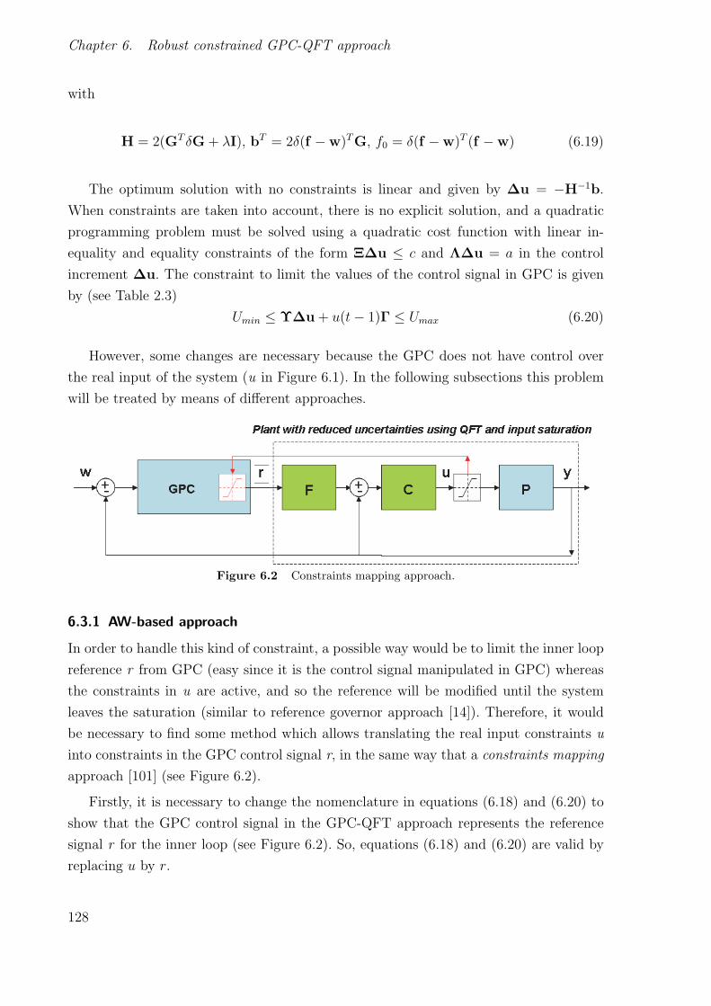
Chapter 6. Robust constrained GPC-QFT approach
with
H = 2(GT δG + λI), bT = 2δ(f − w)TG, f0 = δ(f − w)T (f − w) (6.19)
The optimum solution with no constraints is linear and given by ∆u = −H−1b.
When constraints are taken into account, there is no explicit solution, and a quadratic
programming problem must be solved using a quadratic cost function with linear in-
equality and equality constraints of the form Ξ∆u ≤ c and Λ∆u = a in the control
increment ∆u. The constraint to limit the values of the control signal in GPC is given
by (see Table 2.3)
Umin ≤ Υ∆u + u(t− 1)Γ ≤ Umax (6.20)
However, some changes are necessary because the GPC does not have control over
the real input of the system (u in Figure 6.1). In the following subsections this problem
will be treated by means of different approaches.
Figure 6.2 Constraints mapping approach.
6.3.1 AW-based approach
In order to handle this kind of constraint, a possible way would be to limit the inner loop
reference r from GPC (easy since it is the control signal manipulated in GPC) whereas
the constraints in u are active, and so the reference will be modified until the system
leaves the saturation (similar to reference governor approach [14]). Therefore, it would
be necessary to find some method which allows translating the real input constraints u
into constraints in the GPC control signal r, in the same way that a constraints mapping
approach [101] (see Figure 6.2).
Firstly, it is necessary to change the nomenclature in equations (6.18) and (6.20) to
show that the GPC control signal in the GPC-QFT approach represents the reference
signal r for the inner loop (see Figure 6.2). So, equations (6.18) and (6.20) are valid by
replacing u by r.
128

6.3.1 AW-based approach
Figure 6.3 Input constraint in GPC-QFT approach.
The proposed idea in order to face the constrained problem is based on the AW
technique (see Figure 2.2). As is well-known, in the AW schemes the system remains free
whereas the saturation is not active. However, when saturation occurs, the integral term
in the controller is modified up to the system is out of the saturation limit, where the
modification of the integral element is not performed instantaneously but dynamically
with a time constant Tt [5].
The new constrained structure in GPC-QFT works in the same way that AW, but
instead of reducing the effect of the integral term, the future reference is modified in
order to let the system leaves the saturation limit. Figure 6.3 shows the block diagram
for this approach, where the proposed idea will be studied to see how the system can
also face load disturbances.
Therefore, the reference is not modified while the system is out of the saturation
limits working in a linear way as shown in the previous sections. However, when satura-
tion occurs, the future reference is softened including future constraints from predictive
control using equations (6.18), (6.20). These future constraints are calculated modify-
ing the future references obtained at the previous time instant, being this modification
proportional to the difference between the control signal and the saturation limit. The
control signal saturation is given by
u(k) =
⎧⎪⎪⎪⎨⎪⎪⎪⎩
Umin if u(k) ≤ Umin
u(k) if Umin ≤ u(k) ≤ Umax
Umax if u(k) ≥ Umax
(6.21)
where [Umin, Umax] define the saturation limits, u(k) is the current control signal, and
u(k) the saturated control signal. So, when the saturation is active the future constraints
129

Chapter 6. Robust constrained GPC-QFT approach
on the reference [rmin, rmax] are calculated as follows
rmax =
⎧⎨⎩ rk(1 + diff
α) if diff < 0
∞ if diff >= 0(6.22)
rmin =
⎧⎨⎩ rk(1 + diff
α) if diff > 0
−∞ if diff <= 0(6.23)
rk = r(k|k), r(k + 1|k), ..., r(k + Nu − 1|k) (6.24)
rk = r(k + 1|k), ..., r(k + Nu − 1|k), r(k + Nu − 1|k)︸ ︷︷ ︸ (6.25)
being diff = u(k) − u(k), α a free parameter used to adjust the influence of diff over
the modifications in the reference (notice that an exponential profile could be used for
this parameter to weight in a different way different values of future references), rk are
the future references calculated from GPC at instant time k (calculated without taking
constraints into account, that is, for the unconstrained case), and rk represents the same
values that rk but without the first element r(k|k) since this is the current reference
signal. Therefore, rk is composed by the last i = 2...Nu − 1 elements of rk with the
last one duplicated (it is considered that the reference remains constant during the last
instant time), to fit Nu elements.
So, in order to perform this approach, a new step is added to the predictive control
algorithm, where the future limits [rmin, rmax] are calculated at each instant time being
applied to the optimization problem (6.18) as follows
min∆r
J(∆r) (6.26)
s.t. rmin ≤ Υ∆r + r(t− 1)Γ ≤ rmax
As shown in equations (6.22) and (6.23) the reference constraints can be made more or
less aggressive by modifying the α parameter. For large values the system gets closer
to the typical saturation (clipping), and the system leaves the saturation as fast as the
values are smaller. In order to avoid great changes in future references, α should be ≥ 1.
For values < 1 the saturation is left faster, but large modifications are performed in the
130

6.3.2 Worst case identification approach
future references and the system could be far from the real future reference w.
An heuristic rule to define α parameter is given by the following equation
α =tsatTm
· diffmax (6.27)
being diffmax the maximum difference between the saturation value and the control
signal for all plants in Π∗, tsat is the maximum time that the control signal is in saturation
for all plants in Π∗, and Tm the sample time. These parameters (diffmax and tsat) can
be calculated by simulating the behavior of all selected plants in Π∗ during the design
stage of the algorithm. A numerical example about the α tuning will be shown in the
examples section.
6.3.2 Worst case identification approach
The previous approach and the reference governor techniques are based on modifying
the set-point in order to release the system from the saturation. In the same way, the
relation between the set-point and the control signal (given from the Gang of Six (2.19)),
could be used in order to implement the same idea. Such relation is given by
Gu,r(s) =U(s)
R(s)=
F (s)C(s)
1 + P (s)C(s)(6.28)
being the discrete version of this transfer function obtained as
Gu,r(z−1) =
U(z−1)
R(z−1)=
F (z−1)C(z−1)
1 + P (z−1)C(z−1)=
b0 + b1z−1 + · · · + bn−1z
−n−1 + bnz−n
1 + a1z−1 + · · · + am−1z−m−1 + amz−m(6.29)
where n < m.
In the context of saturation, it would be necessary to calculate reference values that
keep the system out of it. Therefore, supposing that the set-point is known and the
system is perfectly modelled, the saturated control signal can be calculated off-line using
u(k) = b0r(k) + b1r(k − 1) · · · + bnr(k − n) − a1u(k − 1) − · · · − amu(k −m) (6.30)
u(k) fitting 6.21.
Once the saturated control signal is obtained, the reference modifications necessary
131
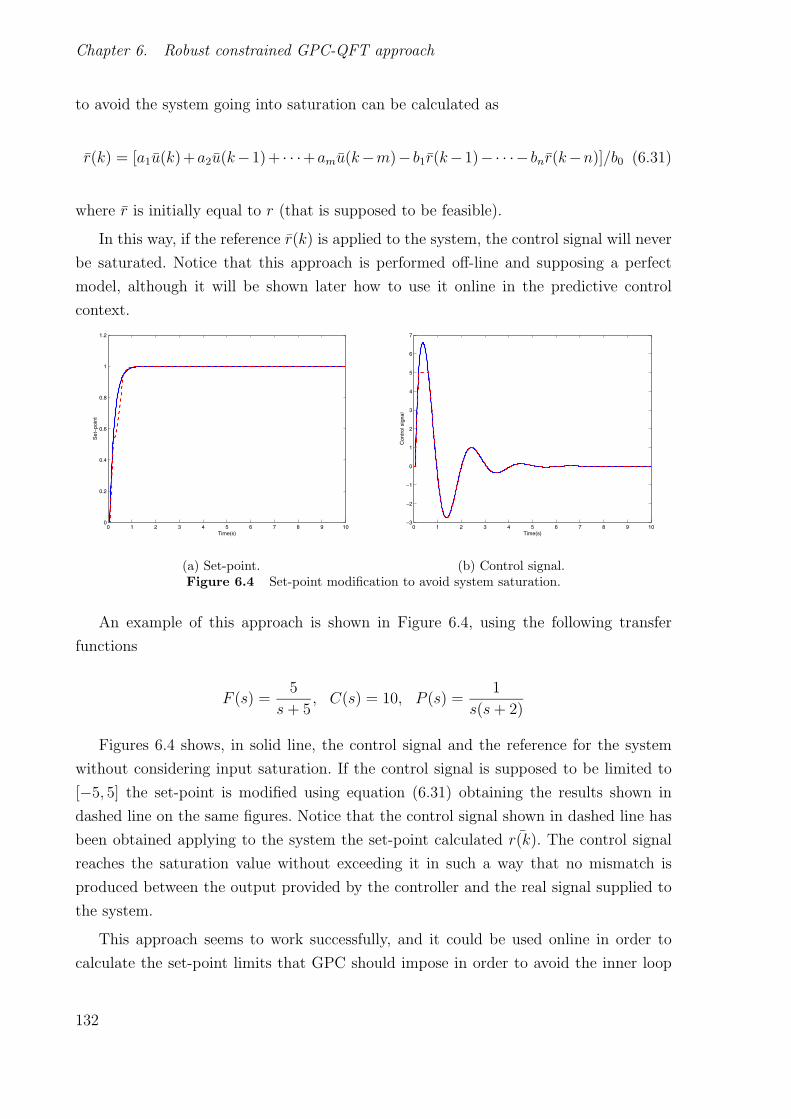
Chapter 6. Robust constrained GPC-QFT approach
to avoid the system going into saturation can be calculated as
r(k) = [a1u(k)+a2u(k−1)+ · · ·+amu(k−m)− b1r(k−1)−· · ·− bnr(k−n)]/b0 (6.31)
where r is initially equal to r (that is supposed to be feasible).
In this way, if the reference r(k) is applied to the system, the control signal will never
be saturated. Notice that this approach is performed off-line and supposing a perfect
model, although it will be shown later how to use it online in the predictive control
context.
0 1 2 3 4 5 6 7 8 9 100
0.2
0.4
0.6
0.8
1
1.2
Time(s)
Set−
poin
t
0 1 2 3 4 5 6 7 8 9 10−3
−2
−1
0
1
2
3
4
5
6
7
Time(s)
Con
trol
sig
nal
(a) Set-point. (b) Control signal.Figure 6.4 Set-point modification to avoid system saturation.
An example of this approach is shown in Figure 6.4, using the following transfer
functions
F (s) =5
s+ 5, C(s) = 10, P (s) =
1
s(s+ 2)
Figures 6.4 shows, in solid line, the control signal and the reference for the system
without considering input saturation. If the control signal is supposed to be limited to
[−5, 5] the set-point is modified using equation (6.31) obtaining the results shown in
dashed line on the same figures. Notice that the control signal shown in dashed line has
been obtained applying to the system the set-point calculated ¯r(k). The control signal
reaches the saturation value without exceeding it in such a way that no mismatch is
produced between the output provided by the controller and the real signal supplied to
the system.
This approach seems to work successfully, and it could be used online in order to
calculate the set-point limits that GPC should impose in order to avoid the inner loop
132

6.3.2 Worst case identification approach
going into saturation. That is, firstly GPC generates the unconstrained future reference
rk to the system at each instant time. These references are used to detect if the inner loop
is saturated in the future by using a perfect model. So, the previous approach could be
used in order to obtain de reference modifications necessary to avoid the saturation. Such
reference modifications would be included as input constraints in the GPC algorithm.
However, the previous approach has only been described for the nominal case where
the process uncertainties are not present. So, the uncertainties must be considered in
order to use this idea in the GPC-QFT approach. The uncertainty in the transfer function
Gu,r(z−1) (6.29) can be represented as dependences on the time domain parameters of
the system. That is, the previous transfer function could be represented as
Gu,r(z−1, θ) =
F (z−1)C(z−1)
1 + P (z−1, θ)C(z−1)(6.32)
where θ ∈ Θ, being Θ a polytope with all possible combinations of the system time
domain parameters (θ comprises κ, i, ζr, βj, ω0j, βr and ω0s parameters in equation (2.6),
with defined bounds that conform the polytope). Then, the transfer function can be
represented in a general way as follows
Gu,r(z−1, θ) =
b0(θ) + b1(θ)z−1 + · · · + bn−1(θ)z
n−1 + bn(θ)zn
1 + a1(θ)z−1 + · · · + am−1(θ)zm−1 + am(θ)zm(6.33)
where n < m.
For the nominal case, the relation between the control signal and the reference was
unique (see equation (6.31)) but now there are so many relations as elements in the plant
family. Therefore, the set-point modifications must be calculated considering the transfer
functions that provokes the maximum and minimum values of the control signal. Once
these transfer functions are detected, the same procedure that in the nominal case can be
performed obtaining the set-point modifications. Notice that if the set-point is reduced
for the transfer function with bigger control signal amplitude, the rest will be reduced
proportionally (since the plants are linear).
Suppose that in the previous example the process transfer function is given by
P (s) =Kp
s(s+ 2), Kp ∈ [0.5, 3]
So, multiple evolutions for the control signal can be obtained as Figure 6.5(a) shows.
133

Chapter 6. Robust constrained GPC-QFT approach
0 1 2 3 4 5 6 7 8 9 10−4
−2
0
2
4
6
8
Time(s)
Con
trol
Sig
nal
0 1 2 3 4 5 6 7 8 9 100
0.2
0.4
0.6
0.8
1
1.2
Time(s)
Set−
poin
t
(a) Unconstrained control signal. (b) Worst case set-point modification.
0 1 2 3 4 5 6 7 8 9 10−3
−2
−1
0
1
2
3
4
5
6
Time(s)
Con
trol
sig
nal
(c) Control signal using the modified set-point.Figure 6.5 Set-point modification for an uncertainty system.
The maximum value of the control signal is obtained for the transfer function with
Kp = 0.5. Then, the set-point is modified based on the control signal of this transfer
function as shown in Figure 6.5(b). If the modified set-point is applied on all the plants,
the control signals keep unsaturated (see Figure 6.5(c)). Notice that the maximum values
of the control signal are not always obtained for the same transfer function (see instant
time t = 1.5). Therefore, the transfer function which produces the maximum control
signal must be identified at each time instant in order to implement this approach online.
The approach can be used in the mixed GPC-QFT approach in order to consider
input saturation. The idea is to detect, at each sample time, those transfer functions
giving the most energetic control signal (upper and lower values) in the inner loop. So,
these transfer functions are used to calculate the set-point modifications necessary to
avoid saturation. Such modifications are considered as constraint limits by GPC, thus
restricting the set-point values and so limiting the control signal u. Therefore, in order
134
6.3.2 Worst case identification approach
to implement this approach, the predictive control algorithm is modified including a new
step where the future set-point limits [rmin, rmax] are calculated at each sample time,
being applied to the optimization problem (6.18). This step is described by the following
algorithm:
1. Worst plants identification. Firstly, the plants defined by equation (6.33) providing
the most energetic control signals along the prediction horizon are identified (that
is, the parameters θ producing the largest future values of the control signals are
estimated). Using the predictive control algorithm, the future references for the
inner loop rk are calculated at each sample time using the nominal plant (see
Figure 6.1). So, the calculated future reference is applied to the uncertain system
in order to identify the worst case plant plants from the amplitude control point
of view. The future control signals of the system can be derived from (6.33)
uk+j = b0(θ)rk+j + b1(θ)rk+j−1 + · · · + bn−1(θ)rk+j−n−1 + bn(θ)rk+j−n − (6.34)
−a1(θ)uk+j−1 − · · · − am−1(θ)uk+j−m−1 − am(θ)uk+j−m
for j = 0...N-1 and where uk denotes u(k) for the sake of simplicity.
Then, at each sampling time, the future control signals depend on the known
future references and the unknown parameters of the model (that depend on the
continuous time bounded model parameters described in (2.6)). Thus, in compact
form, (6.34) can be written as:
uk = (rk, θ) (6.35)
uk = [uk, uk+1, . . . , uk+N−1]T .
Then, the transfer function parameters that produce the maximum and minimum
values of the control signal along the control horizon θmax and θmin, are obtained
as
θmax = maxθ
(rk, θ), θmin = minθ
(rk, θ)
where the optimization involves discretization of the continuous time transfer func-
tions (providing (6.33)) and the on-line solution of a constrained nonlinear program-
ming problem using Sequential Quadratic Programming (SQP).
135
Chapter 6. Robust constrained GPC-QFT approach
2. Set-point limits calculation. Firstly, the future control sequence uk is calculated
using rk (see equation (6.34)) and the worst case model parameters obtained in
the previous step. Then uk is computed considering upper and lower limits in
the control signal Umax and Umin. With the saturated values of the future control
signals, the future constraints on the references rmax and rmin can be easily obtained
using the affine relationship between rk and uk. If the future control signal is
unsaturated the maximum limit for the set-point is considered as rmax = ∞ (or
rmax = −∞ when considering the minimum limit). Then, the actual reference can
be applied to the system using a receding horizon approach.
The proposed approach provides a good solution to avoid the system going into
saturation in presence of uncertainties, as will be shown by means of several examples in
the next section. Notice that the set-point modification is performed for the worst transfer
function (from the maximum control signal point of view) where great differences with
the nominal plant could be obtained, and a high computational load is required.
6.3.3 Hard constraints approach
The affine relation between the control signal and the reference used above can be con-
sidered to express an affine relation between u and ∆r (see Figure 6.1). So, if this relation
is taken into account
u(i) = mTi ∆r + di, i = 1, . . . , Nu (6.36)
the constraints on the control signal u can be expressed as hard constraints on ∆r
substituting such affine relation in equation (6.20). Therefore, the optimization problem
in the GPC-QFT approach considering input saturation could be expressed as
min∆r
J(∆r)
s.t. mTi ∆r + di − Umax ≤ 0, i = 1, . . . , Nu
−mTi ∆r − di + Umin ≤ 0, i = 1, . . . , Nu
Notice that as commented in the previous section, the affine relation between u and r
is not unique due to the presence of uncertainties. So, it would be necessary to consider
136
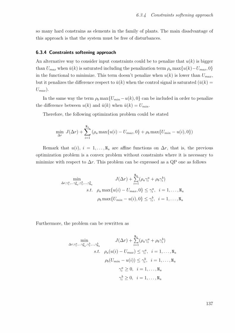
6.3.4 Constraints softening approach
so many hard constrains as elements in the family of plants. The main disadvantage of
this approach is that the system must be free of disturbances.
6.3.4 Constraints softening approach
An alternative way to consider input constraints could be to penalize that u(k) is bigger
than Umax when u(k) is saturated including the penalization term ρa maxu(k)−Umax, 0in the functional to minimize. This term doesn’t penalize when u(k) is lower than Umax,
but it penalizes the difference respect to u(k) when the control signal is saturated (u(k) =
Umax).
In the same way the term ρb maxUmin−u(k), 0 can be included in order to penalize
the difference between u(k) and u(k) when u(k) = Umin.
Therefore, the following optimization problem could be stated
min∆r
J(∆r) +Nu∑i=1
(ρa maxu(i) − Umax, 0 + ρb maxUmin − u(i), 0)
Remark that u(i), i = 1, . . . , Nu are affine functions on ∆r, that is, the previous
optimization problem is a convex problem without constraints where it is necessary to
minimize with respect to ∆r. This problem can be expressed as a QP one as follows
min∆r,γa
1 ,...γaNu,γb
1,...,γbNu
J(∆r) +Nu∑i=1
(ρaγai + ρbγ
bi )
s.t. ρa maxu(i) − Umax, 0 ≤ γai , i = 1, . . . , Nu
ρb maxUmin − u(i), 0 ≤ γbi , i = 1, . . . , Nu
Furthermore, the problem can be rewritten as
min∆r,γa
1 ,...γaNu,γb
1,...,γbNu
J(∆r) +Nu∑i=1
(ρaγai + ρbγ
bi )
s.t. ρa(u(i) − Umax) ≤ γai , i = 1, . . . , Nu
ρb(Umin − u(i)) ≤ γbi , i = 1, . . . , Nu
γai ≥ 0, i = 1, . . . , Nu
γbi ≥ 0, i = 1, . . . , Nu
137

Chapter 6. Robust constrained GPC-QFT approach
Finally, remember that u(i) depends affinely with respect to ∆r as commented above
(6.36). Then, the optimization problem can be written as
min∆r,γa
1 ,...γaNu,γb
1,...,γbNu
J(∆r) +Nu∑i=1
(ρaγai + ρbγ
bi )
s.t. ρa(mTi ∆r + di − Umax) ≤ γai , i = 1, . . . , Nu
ρb(Umin −mTi ∆r − di) ≤ γbi , i = 1, . . . , Nu
γai ≥ 0, i = 1, . . . , Nu
γbi ≥ 0, i = 1, . . . , Nu
Therefore, the problem of penalizing the difference between u(k) and u(k) can be ex-
pressed as a QP problem in ∆r, that presents a great number of decision variables
substantially increasing the computational burden. The same result can be expressed in
an equivalent way using the ideas proposed by [107], so reducing the number of variables
to minimize in the following way
min∆r,
J(∆r) +
s.t. (mTi ∆r + di − Umax) ≤ ηa, i = 1, . . . , Nu
(Umin −mTi ∆r − di) ≤ ηb, i = 1, . . . , Nu
≥ 0, i = 1, . . . , Nu
Notice that as in the previous approach, it would be necessary to consider so many hard
constrains as elements in the family of plants due to the system uncertainties.
6.4 Numerical Examples
6.4.1 Unconstrained Example
A very simple example will be used to demonstrate the feature of the GPC-QFT approach
when constraints are not present. In order to perform the simulations the SISO-GPCIT
138

6.4.1 Unconstrained Example
0 0.5 1 1.5 2 2.5 3 3.5 40
0.5
1
1.5
Time (s)
All
ou
tpu
ts
Figure 6.6 Nominal GPC for (N1, N2, Nu, δ, λ) = (1, 4, 4, 1, 0.1).
[58] and SISO-QFTIT [34, 33] tools have been used. The system is given by
P (s) =b
s+ a; b ∈ [1, 5]; a ∈ [0.1, 1]
The model for nominal GPC is P0 = 3s+0.5
(in this case not selected using (6.4),
in order to better show the performance improvements of the algorithm). The tuning
parameters have been selected as (N1, N2, Nu, δ, λ) = (1, 4, 4, 1, 0.1) and the sample
time as 0.1. Hence, the elements of characteristic polynomial (2.18) are the following
R(z−1) = 0.6360, S(z−1) = 2.5377 − 1.5377z−1
B(z−1)p = b0z−1, b0 ∈ [0.0952, 0.4975]
A(z−1)p = 1 + a1z−1, a1 ∈ [−0.9048,−0.9901]
The RRL for this system and the output evolution in presence of uncertainties can
be seen in Figure 6.6. As shown, the system remains stable (Theorem 6.1 is fulfilled) in
presence of uncertainties, but the performance is harshly affected.
In order to show the advantages of the GPC-QFT approach, it is necessary to impose
the specifications for designing the controller and prefilter with QFT. The frequency set
for the design has been selected to Ω = [0.01, 0.1, 1, 10] rad/s. The stability specification
is set to Ms = 1 corresponding to a GM ≥ 2 and a PM = 59.35, and for the tracking
specifications the maximum and minimum values for the magnitude have been described
by the next transfer functions
Mu(s) =2
s+ 2Ml(s) =
10
s2 + 7s+ 10
139
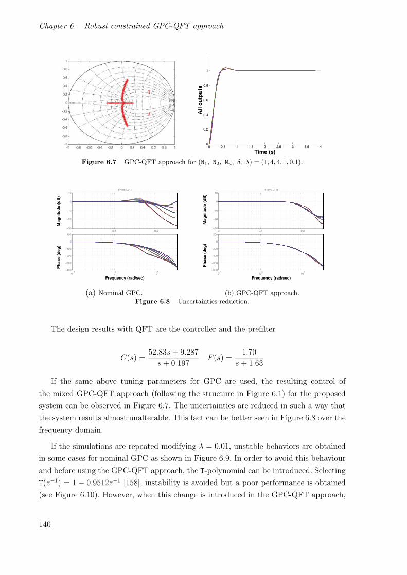
Chapter 6. Robust constrained GPC-QFT approach
0 0.5 1 1.5 2 2.5 3 3.5 40
0.2
0.4
0.6
0.8
1
Time (s)
All
ou
tpu
ts
Figure 6.7 GPC-QFT approach for (N1, N2, Nu, δ, λ) = (1, 4, 4, 1, 0.1).
0 0.1 0.2−30
−20
−10
0
10From: U(1)
10−1
100
101
−400
−300
−200
−100
0
100
Frequency (rad/sec)
Ph
ase
(deg
)
Mag
nit
ud
e (d
B)
0 0.1 0.2−30
−20
−10
0
10From: U(1)
10−1
100
101
−800
−600
−400
−200
0
200
Frequency (rad/sec)
Ph
ase
(deg
)
Mag
nit
ud
e (d
B)
(a) Nominal GPC. (b) GPC-QFT approach.Figure 6.8 Uncertainties reduction.
The design results with QFT are the controller and the prefilter
C(s) =52.83s+ 9.287
s+ 0.197F (s) =
1.70
s+ 1.63
If the same above tuning parameters for GPC are used, the resulting control of
the mixed GPC-QFT approach (following the structure in Figure 6.1) for the proposed
system can be observed in Figure 6.7. The uncertainties are reduced in such a way that
the system results almost unalterable. This fact can be better seen in Figure 6.8 over the
frequency domain.
If the simulations are repeated modifying λ = 0.01, unstable behaviors are obtained
in some cases for nominal GPC as shown in Figure 6.9. In order to avoid this behaviour
and before using the GPC-QFT approach, the T-polynomial can be introduced. Selecting
T(z−1) = 1 − 0.9512z−1 [158], instability is avoided but a poor performance is obtained
(see Figure 6.10). However, when this change is introduced in the GPC-QFT approach,
140
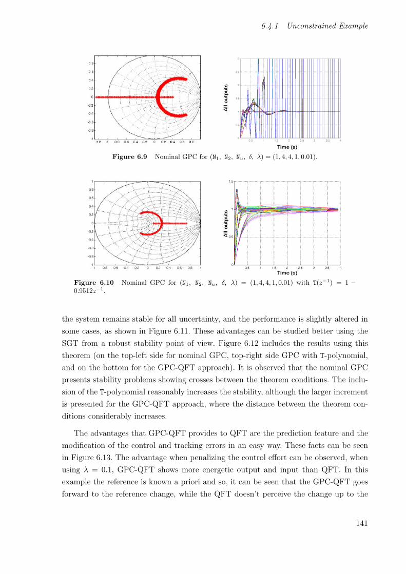
6.4.1 Unconstrained Example
Figure 6.9 Nominal GPC for (N1, N2, Nu, δ, λ) = (1, 4, 4, 1, 0.01).
Figure 6.10 Nominal GPC for (N1, N2, Nu, δ, λ) = (1, 4, 4, 1, 0.01) with T(z−1) = 1 −0.9512z−1.
the system remains stable for all uncertainty, and the performance is slightly altered in
some cases, as shown in Figure 6.11. These advantages can be studied better using the
SGT from a robust stability point of view. Figure 6.12 includes the results using this
theorem (on the top-left side for nominal GPC, top-right side GPC with T-polynomial,
and on the bottom for the GPC-QFT approach). It is observed that the nominal GPC
presents stability problems showing crosses between the theorem conditions. The inclu-
sion of the T-polynomial reasonably increases the stability, although the larger increment
is presented for the GPC-QFT approach, where the distance between the theorem con-
ditions considerably increases.
The advantages that GPC-QFT provides to QFT are the prediction feature and the
modification of the control and tracking errors in an easy way. These facts can be seen
in Figure 6.13. The advantage when penalizing the control effort can be observed, when
using λ = 0.1, GPC-QFT shows more energetic output and input than QFT. In this
example the reference is known a priori and so, it can be seen that the GPC-QFT goes
forward to the reference change, while the QFT doesn’t perceive the change up to the
141

Chapter 6. Robust constrained GPC-QFT approach
Figure 6.11 GPC-QFT approach for (N1, N2, Nu, δ, λ) = (1, 4, 4, 1, 0.01).
instant in which the reference is modified.
10−5
100
105
−200
−150
−100
−50
0
50
Frecuencia (rad/s)
Mag
nit
ud
(d
B)
GPC NOMINAL
10−5
100
105
−200
−150
−100
−50
0
50
Frecuencia (rad/s)
Mag
nit
ud
(d
B)
GPC NOMINAL CON POLINOMIO T
10−5
100
105
−200
−150
−100
−50
0
50
Frecuencia (rad/s)
Mag
nit
ud
(d
B)
GPC−QFT
Figure 6.12 Robust stability using the SGT. The upper curves represent |P ||P | y the lower
ones 1T .
6.4.2 Constrained Example
An integrator plant with uncertainty in the gain has been proposed in order to show how
the proposed control structure manages control signal constraints. The plant is given by
P (s) = Kp
swhere Kp ∈ [1, 10], and being the control signal limited to [−1, 1]. First of
all the QFT design is performed. The frequency set for the design has been selected to
Ω = [0.01, 0.1, 1, 10, 20] rad/s. The stability specification is set to Ms = 1 in the same
way that in the previous example, and for the tracking specifications the maximum and
142

6.4.2 Constrained Example
Figure 6.13 Advantage of prediction feature and control effort. Thick line GPC-QFT, thinline QFT, and dash-dot the reference.
10−1
100
101
102
−30
−25
−20
−15
−10
−5
0
5
Frequency (rad/s)
Mag
nit
ud
e (d
B)
Figure 6.14 Magnitude bands for integrator example.
minimum values for the magnitude have been set from the curves shown in Figure 6.14
(calculated interactively using the tool developed by [34, 33]), being represented by the
next transfer functions
Mu(s) =6
s+ 6Ml(s) =
60
s2 + 17s+ 60
So, the controller and prefilter obtained are described by
C(s) =0.2267s+ 13.84
0.0002331s2 + 0.05145s+ 1F (s) =
1
0.1761s+ 1
The GPC parameters are set to (N1, N2, Nu, δ, λ) = (1, 5, 5, 1, 2), the sample time
equal to 0.01, and the nominal plant Po = 1s. The simulation results without constraints
are shown in Figure 6.15. It can be observed that the control signal is out of the saturation
for a couple of plants with Kp values 1 and 2.
If the typical saturation (clipping) is performed, the results shown in Figure 6.16 are
143
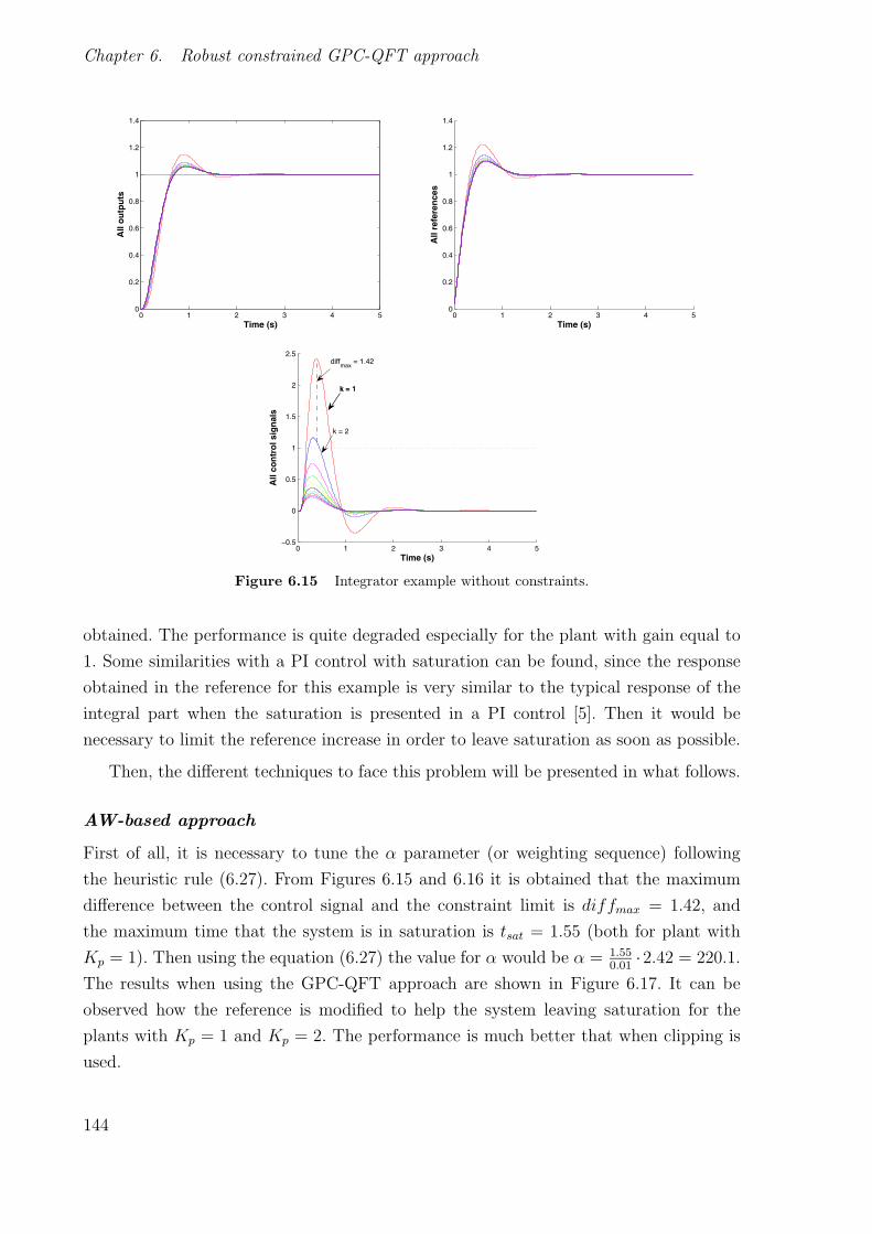
Chapter 6. Robust constrained GPC-QFT approach
0 1 2 3 4 50
0.2
0.4
0.6
0.8
1
1.2
1.4
Time (s)
All
ou
tpu
ts
0 1 2 3 4 50
0.2
0.4
0.6
0.8
1
1.2
1.4
Time (s)
All
refe
ren
ces
0 1 2 3 4 5−0.5
0
0.5
1
1.5
2
2.5
Time (s)
All
con
tro
l sig
nal
s
k = 1k = 1
k = 2
diffmax
= 1.42
Figure 6.15 Integrator example without constraints.
obtained. The performance is quite degraded especially for the plant with gain equal to
1. Some similarities with a PI control with saturation can be found, since the response
obtained in the reference for this example is very similar to the typical response of the
integral part when the saturation is presented in a PI control [5]. Then it would be
necessary to limit the reference increase in order to leave saturation as soon as possible.
Then, the different techniques to face this problem will be presented in what follows.
AW-based approach
First of all, it is necessary to tune the α parameter (or weighting sequence) following
the heuristic rule (6.27). From Figures 6.15 and 6.16 it is obtained that the maximum
difference between the control signal and the constraint limit is diffmax = 1.42, and
the maximum time that the system is in saturation is tsat = 1.55 (both for plant with
Kp = 1). Then using the equation (6.27) the value for α would be α = 1.550.01
·2.42 = 220.1.
The results when using the GPC-QFT approach are shown in Figure 6.17. It can be
observed how the reference is modified to help the system leaving saturation for the
plants with Kp = 1 and Kp = 2. The performance is much better that when clipping is
used.
144
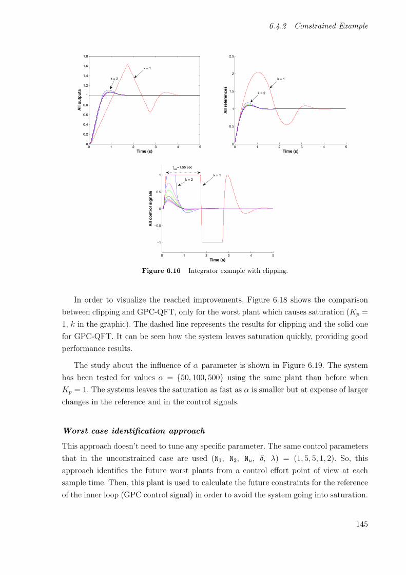
6.4.2 Constrained Example
0 1 2 3 4 50
0.2
0.4
0.6
0.8
1
1.2
1.4
1.6
1.8
Time (s)
All
ou
tpu
ts
k = 1
k = 2
0 1 2 3 4 50
0.5
1
1.5
2
2.5
Time (s)
All
refe
ren
ces
k = 1
k = 2
0 1 2 3 4 5
−1
−0.5
0
0.5
1
Time (s)
All
con
tro
l sig
nal
s
k = 1k = 2
tsat
=1.55 sec
Figure 6.16 Integrator example with clipping.
In order to visualize the reached improvements, Figure 6.18 shows the comparison
between clipping and GPC-QFT, only for the worst plant which causes saturation (Kp =
1, k in the graphic). The dashed line represents the results for clipping and the solid one
for GPC-QFT. It can be seen how the system leaves saturation quickly, providing good
performance results.
The study about the influence of α parameter is shown in Figure 6.19. The system
has been tested for values α = 50, 100, 500 using the same plant than before when
Kp = 1. The systems leaves the saturation as fast as α is smaller but at expense of larger
changes in the reference and in the control signals.
Worst case identification approach
This approach doesn’t need to tune any specific parameter. The same control parameters
that in the unconstrained case are used (N1, N2, Nu, δ, λ) = (1, 5, 5, 1, 2). So, this
approach identifies the future worst plants from a control effort point of view at each
sample time. Then, this plant is used to calculate the future constraints for the reference
of the inner loop (GPC control signal) in order to avoid the system going into saturation.
145

Chapter 6. Robust constrained GPC-QFT approach
0 1 2 3 4 50
0.2
0.4
0.6
0.8
1
1.2
1.4
Time(s)
All
ou
tpu
ts
k = 1k = 2
0 1 2 3 4 50
0.2
0.4
0.6
0.8
1
1.2
1.4
Time(s)
All
refe
ren
ces
k = 1k = 2
0 1 2 3 4 5−0.2
0
0.2
0.4
0.6
0.8
1
1.2
Time(s)
All
con
tro
l sig
nal
s
k = 1
k = 2
Figure 6.17 Integrator example with GPC-QFT approach.
Figure 6.20 shows the results of applying this approach. The responses are very
similar to those obtained with the previous approach. Notice that it seems that the
control signal is saturated during one second more or less, but really it never exceeds the
saturation limit. Figure 6.21 shows the comparison between clipping and the worst case
identification approach (the example is shown for the worst plant with Kp = 1, k in the
figure, from a saturation point of view).
Hard constraints approach
This approach, as commented before, consists in adding an intermediate step in the
predictive control algorithm in order to allow performing the constraint mapping. The
constraints are calculated imposing limits on ∆r regarding the affine relation between
this signal and u. Therefore, the design presented in the previous simulations would be
the same for this case, only modifying the way in which the constraints are calculated.
The results obtained for this approach are shown in Figure 6.22. Figure 6.23 shows the
comparison between using typical clipping and the hard constraint approach for the
worst plant with Kp = 1 (k in the figure).
146

6.4.2 Constrained Example
0 1 2 3 4 50
0.2
0.4
0.6
0.8
1
1.2
1.4
1.6
1.8
Time(s)
All
ou
tpu
ts
0 1 2 3 4 50
0.5
1
1.5
2
2.5
Time(s)
All
refe
ren
ces
0 1 2 3 4 5
−1
−0.8
−0.6
−0.4
−0.2
0
0.2
0.4
0.6
0.8
1
Time(s)
All
con
tro
l sig
nal
s
Figure 6.18 Clipping constraints (dashed) versus GPC-QFT approach (solid).
Soft constraints approach
In the case of constraints softening, as in the previous approach, the design performed
for the GPC-QFT approach without considering constraints is reutilized. The weighting
factors have been set to ηa = ηb = 0.05 in the simulations. The results for this approach
can be observed in Figure 6.24. In order to better analyze the advantages of this approx-
imation over the clipping results, both approaches are shown in Figure 6.25 for the worst
saturation case (Kp = 1).
Comparison of the different approaches
From the results obtained above, similar behaviors can be observed for all of them.
Figure 6.26 shows a comparison where the four approaches are simulated for the worst
case from a control effort point of view (Kp = 1).
The main difference to note is that for the AW-based approach, the control signal
is saturated while in the rest it never exceeds the saturation limit (for the worst case
identification approach, the control signal never exceeds of the saturation limit). This
fact is very important from a GPC point of view, since internally GPC supposes that
147

Chapter 6. Robust constrained GPC-QFT approach
0 1 2 3 4 50
0.2
0.4
0.6
0.8
1
1.2
1.4
Time(s)
All
ou
tpu
ts
0 1 2 3 4 50
0.5
1
1.5
All
refe
ren
ces
All
refe
ren
ces
0.2 0.4 0.6 0.8 1 1.2
0.2
0.4
0.6
0.8
1
Time(s)
α = 50 α = 100
α = 500
0 1 2 3 4 5−0.5
0
0.5
1
0.2 0.4 0.6 0.8 1 1.2 1.4
0.4
0.6
0.8
1
Time(s)
All
con
tro
l sig
nal
sA
ll co
ntr
ol s
ign
als
α = 50
α = 100
α = 500
Figure 6.19 Effect of α parameter in the constraint management.
the model is working in linear mode without saturation. So, at the moment in which the
control signal u is in saturation, great differences between the prediction and the real
results could appear. However, for stable systems, this difference can be removed by the
receding horizon strategy.
On the other hand, it is necessary to consider that the hard constraint, and con-
straints softening approaches could present feasibility problems in presence of distur-
bances. Notice that these approaches include constraints information directly based on
the linear relation between u and r, where the presence of disturbances breaks such rela-
tion incorporating large errors. However, for the AW-based and worst case identification
approaches the disturbances can be attenuated perfectly. Next section shows an example
to remark this problem.
6.4.3 Load disturbances
Disturbances are one of the relevant aspects of the control problems. In fact, without
disturbances and process uncertainty there would be no need for feedback [5]. A load
disturbance at instant time t = 5 seconds with a value of -0.9 (for a value of -1 the system
goes into saturation all the time) has been introduced in the previous example in order
148
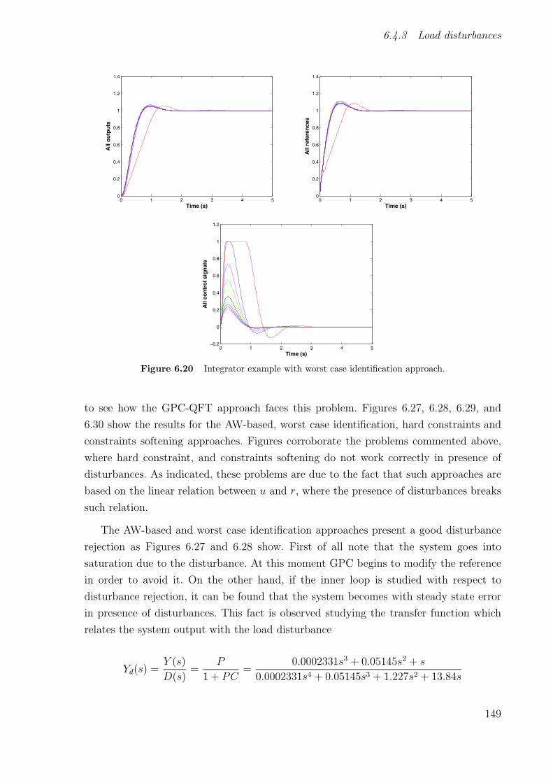
6.4.3 Load disturbances
0 1 2 3 4 50
0.2
0.4
0.6
0.8
1
1.2
1.4
Time (s)
All
ou
tpu
ts
0 1 2 3 4 50
0.2
0.4
0.6
0.8
1
1.2
1.4
Time (s)
All
refe
ren
ces
0 1 2 3 4 5−0.2
0
0.2
0.4
0.6
0.8
1
1.2
Time (s)
All
con
tro
l sig
nal
s
Figure 6.20 Integrator example with worst case identification approach.
to see how the GPC-QFT approach faces this problem. Figures 6.27, 6.28, 6.29, and
6.30 show the results for the AW-based, worst case identification, hard constraints and
constraints softening approaches. Figures corroborate the problems commented above,
where hard constraint, and constraints softening do not work correctly in presence of
disturbances. As indicated, these problems are due to the fact that such approaches are
based on the linear relation between u and r, where the presence of disturbances breaks
such relation.
The AW-based and worst case identification approaches present a good disturbance
rejection as Figures 6.27 and 6.28 show. First of all note that the system goes into
saturation due to the disturbance. At this moment GPC begins to modify the reference
in order to avoid it. On the other hand, if the inner loop is studied with respect to
disturbance rejection, it can be found that the system becomes with steady state error
in presence of disturbances. This fact is observed studying the transfer function which
relates the system output with the load disturbance
Yd(s) =Y (s)
D(s)=
P
1 + PC=
0.0002331s3 + 0.05145s2 + s
0.0002331s4 + 0.05145s3 + 1.227s2 + 13.84s
149

Chapter 6. Robust constrained GPC-QFT approach
0 1 2 3 4 50
0.2
0.4
0.6
0.8
1
1.2
1.4
1.6
1.8
Time (s)
All
ou
tpu
ts
0 1 2 3 4 50
0.5
1
1.5
2
2.5
Time (s)
All
refe
ren
ces
0 1 2 3 4 5
−1
−0.8
−0.6
−0.4
−0.2
0
0.2
0.4
0.6
0.8
1
Time (s)
All
con
tro
l sig
nal
s
Figure 6.21 Clipping constraint (dashed) versus GPC-QFT with worst case identification(solid).
0 1 2 3 4 50
0.2
0.4
0.6
0.8
1
1.2
1.4
Time (s)
All
Ou
tpu
ts
0 1 2 3 4 50
0.2
0.4
0.6
0.8
1
1.2
1.4
Time (s)
All
Ref
eren
ces
0 1 2 3 4 5−0.2
0
0.2
0.4
0.6
0.8
1
1.2
Time (s)
All
Co
ntr
ol S
ign
als
Figure 6.22 Integrator example for the GPC-QFT approach with hard constraints.
150

6.4.3 Load disturbances
0 1 2 3 4 50
0.2
0.4
0.6
0.8
1
1.2
1.4
1.6
1.8
Time (s)
All
Ou
tpu
ts
0 1 2 3 4 50
0.5
1
1.5
2
2.5
Time (s)
All
Ref
eren
ces
0 1 2 3 4 5
−1
−0.8
−0.6
−0.4
−0.2
0
0.2
0.4
0.6
0.8
1
Time (s)
All
Co
ntr
ol S
ign
als
Figure 6.23 Clipping constraint (dashed) versus GPC-QFT with hard constraints (solid).
0 1 2 3 4 50
0.2
0.4
0.6
0.8
1
1.2
1.4
Time (s)
All
Ou
tpu
ts
0 1 2 3 4 50
0.2
0.4
0.6
0.8
1
1.2
1.4
Time (s)
All
Ref
eren
ces
0 1 2 3 4 5−0.2
0
0.2
0.4
0.6
0.8
1
1.2
Time (s)
All
Co
ntr
ol S
ign
als
Figure 6.24 Integrator example for the GPC-QFT approach with constraints softening, ηa =ηb = 0.05.
where ed = Yd(0) 0.07225. This means that the inner loop would have a steady state
error of ed · d, being d the disturbance value.
However, as figures show the steady state error for the GPC-QFT approach is zero.
This is due to the integrator ability which GPC contributes thanks to use a CARIMA
151

Chapter 6. Robust constrained GPC-QFT approach
0 1 2 3 4 50
0.2
0.4
0.6
0.8
1
1.2
1.4
1.6
1.8
Time (s)
All
Ou
tpu
ts
0 1 2 3 4 50
0.5
1
1.5
2
2.5
Time (s)
All
Ref
eren
ces
0 1 2 3 4 5
−1
−0.8
−0.6
−0.4
−0.2
0
0.2
0.4
0.6
0.8
1
Time (s)
All
Co
ntr
ol S
ign
als
Figure 6.25 Clipping constraint (dashed) versus GPC-QFT with constraints softening (solid).
0 1 2 3 4 50
0.2
0.4
0.6
0.8
1
1.2
1.4
Time (s)
All
Ou
tpu
ts
Constraint SoftingHard constraintAnti−windupWorst Ident
0 1 2 3 4 50
0.2
0.4
0.6
0.8
1
1.2
1.4
Time (s)
All
Ref
eren
ces
Constraint SoftingHard constraintAnti−windupWorst Identification
0 1 2 3 4 5−0.2
0
0.2
0.4
0.6
0.8
1
1.2
Time (s)
All
Co
ntr
ol S
ign
als
Constraint SoftingHard constraintAnti−windupWorst Ident
Figure 6.26 Comparison of the different approaches.
model (2.7). From Figures 6.27 and 6.28 it can be observed how GPC augments the
reference so that the steady state error of the inner loop is eliminated.
152

6.5 RGPCQFT-IT
0 2 4 6 8 100
0.2
0.4
0.6
0.8
1
1.2
1.4
Time (s)
All
ou
tpu
ts
0 2 4 6 8 100
0.2
0.4
0.6
0.8
1
1.2
1.4
Time (s)
All
refe
ren
ces
0 2 4 6 8 10−0.2
0
0.2
0.4
0.6
0.8
1
1.2
Time (s)
All
con
tro
l sig
nal
s
Figure 6.27 AW-based approach in presence of load disturbances.
0 2 4 6 8 100
0.2
0.4
0.6
0.8
1
1.2
1.4
Time (s)
All
ou
tpu
ts
0 2 4 6 8 100
0.2
0.4
0.6
0.8
1
1.2
1.4
Time (s)
All
refe
ren
ces
0 2 4 6 8 10−0.2
0
0.2
0.4
0.6
0.8
1
1.2
Time (s)
All
con
tro
l sig
nal
s
Figure 6.28 Worst case identification approach in presence of load disturbances.
6.5 RGPCQFT-IT
RGPCQFT-IT is an interactive tool which implements the GPC-QFT approach in order
to serve both for educational, research, and industrial application purposes, due to the
153
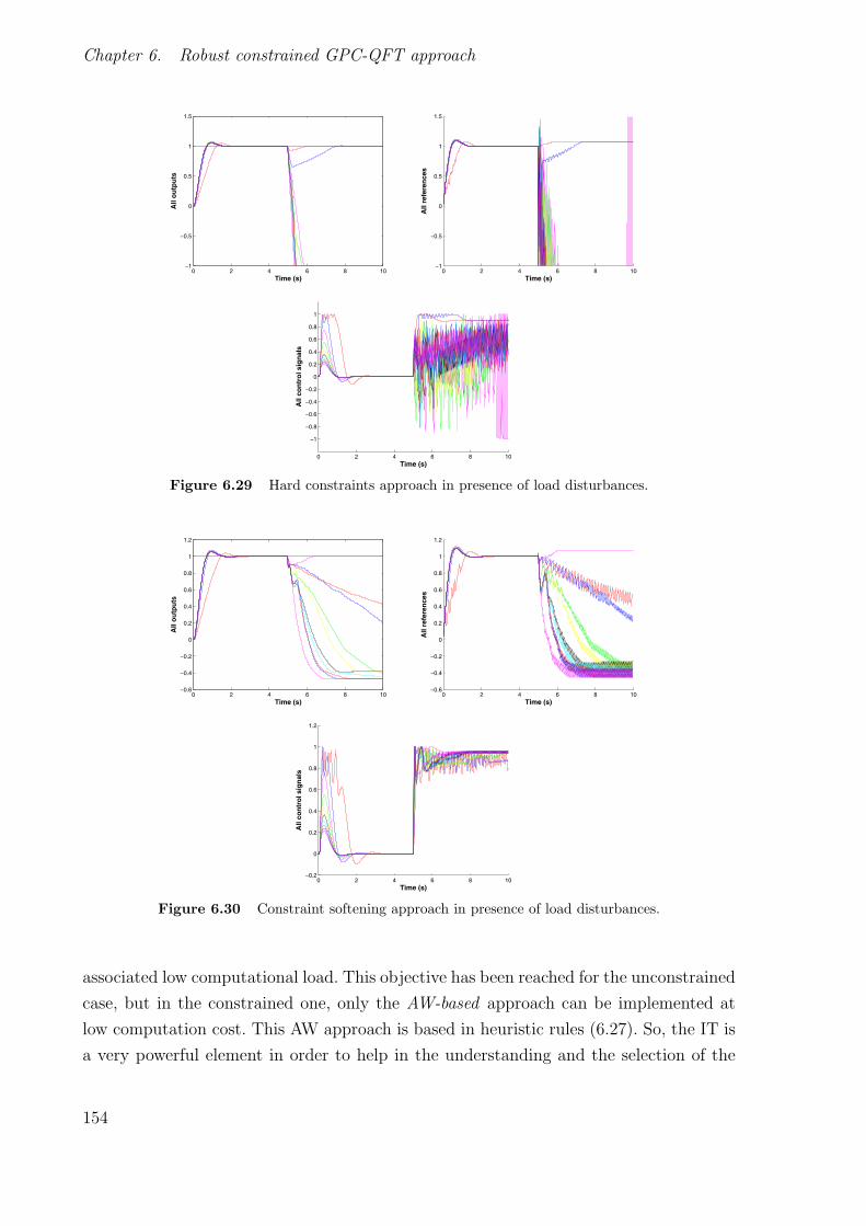
Chapter 6. Robust constrained GPC-QFT approach
0 2 4 6 8 10−1
−0.5
0
0.5
1
1.5
Time (s)
All
ou
tpu
ts
0 2 4 6 8 10−1
−0.5
0
0.5
1
1.5
Time (s)
All
refe
ren
ces
0 2 4 6 8 10
−1
−0.8
−0.6
−0.4
−0.2
0
0.2
0.4
0.6
0.8
1
Time (s)
All
con
tro
l sig
nal
s
Figure 6.29 Hard constraints approach in presence of load disturbances.
0 2 4 6 8 10−0.6
−0.4
−0.2
0
0.2
0.4
0.6
0.8
1
1.2
Time (s)
All
ou
tpu
ts
0 2 4 6 8 10−0.6
−0.4
−0.2
0
0.2
0.4
0.6
0.8
1
1.2
Time (s)
All
refe
ren
ces
0 2 4 6 8 10−0.2
0
0.2
0.4
0.6
0.8
1
1.2
Time (s)
All
con
tro
l sig
nal
s
Figure 6.30 Constraint softening approach in presence of load disturbances.
associated low computational load. This objective has been reached for the unconstrained
case, but in the constrained one, only the AW-based approach can be implemented at
low computation cost. This AW approach is based in heuristic rules (6.27). So, the IT is
a very powerful element in order to help in the understanding and the selection of the
154

6.5.1 Description of the Interactive Tool
Figure 6.31 RGPCQFT-IT main window. All the features of the GPC-QFT approach canbe interactively visualized and modified on the screen.
heuristic parameters.
By using RGPCQFT-IT, the user can include a precalculated inner control loop, that
can be designed using QFT, being the IT open to any other robust control technique
implementing a 2-DOF control scheme. Once the inner control loop is defined, the user
can tune the predictive control parameters in the same way that in SISO-GPCIT and
MIMO-GPCIT. The robust stability can interactively be observed using an approxi-
mated representation of the RRL. The user can calculate the heuristic parameters for
the constrained case and compare the results with the typical clipping solution.
Notice that the predictive control algorithm is the same that such implemented in
the previous IT, only including new steps in order to perform the constraint mapping
approach. In this way, the IT has a lot of features similar to the previous ones; thus, only
the most important interactive elements will be described.
6.5.1 Description of the Interactive Tool
This section briefly describes the main aspects of RGPCQFT-IT. The main screen of the
tool is shown in Figure 6.31.
155

Chapter 6. Robust constrained GPC-QFT approach
Process parameters
It is the zone of the IT available to modify the parameters of the process. It is very
similar to the process parameter zone in PID LoopShaping (see Figure 4.17) where the
user can modify the process transfer function using a pole-zero interactive graphic in
the s-plane, and playing on several sliders. The main differences is that it is possible to
modify the parameters and the respective uncertainty limits. An example for a second
order system (P (s) = Kp/s(s+a)) is shown in Figure 6.31. The sliders knom and knomp
allow defining the static gain of the nominal model and the plant respectively. The limits
for a are graphically represented in the graphic Transfer function, interactively being
possible to modify them.
Control parameters
As in SISO-GPCIT and MIMO-GPCIT, this area allows modifying the weighting factors
Delta and Lambda of the predictive control algorithm, the sample time (Tm), the end
time (Nend), and the number of set-point steps (SP). On the other hand, it is possible to
activate input constraints (Constrained) and the constraint mapping options (Mapping),
being also available the modification of the heuristic factor α (alpha).
RRL graphic
Located below the Control parameters zone, this graphic shows an approximated repre-
sentation of the RRL for the unconstrained system, to study the robust stability inter-
actively.
Graphics
The graphics are located on the right hand side of the tool. The graphics follow the
same philosophy that in the rest of IT. The Process Output graphic shows the system
output being possible to modify the prediction horizons, the set-point value, and the load
disturbances in an interactive way. The GPC output (the reference for the inner loop)
is shown in the GPC Output graphic, where the control horizon can be modified using a
vertical interactive line. The Control signal graphic shows the real control signal of the
system. From this graphic the user can interactively modify the saturation limits using
two horizontal lines. The vertical and horizontal scales of the graphics can be modified
using three black triangles available on the graphics (, ).
The interactive tool allows comparing clipping versus constraints mapping approaches
using the Mapping option available at Control parameters zone. The heuristic parameters
tsat and diffmax can be calculated based on the vertical pink and red lines.
156
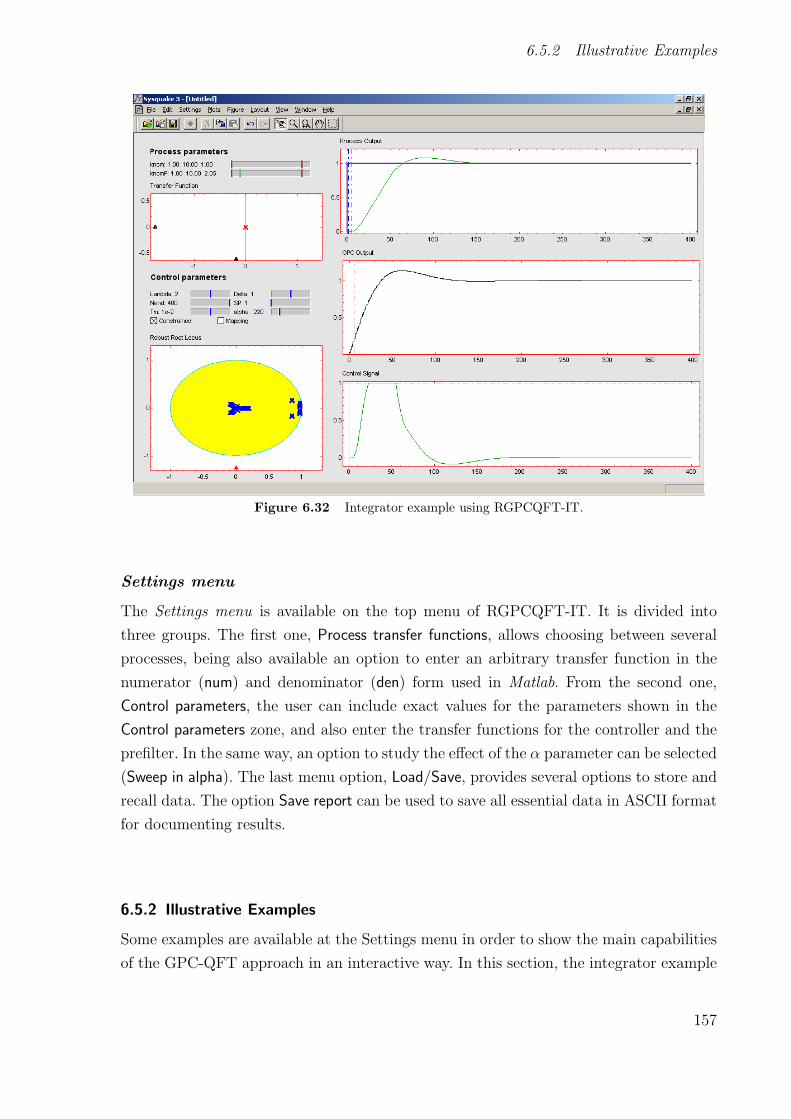
6.5.2 Illustrative Examples
Figure 6.32 Integrator example using RGPCQFT-IT.
Settings menu
The Settings menu is available on the top menu of RGPCQFT-IT. It is divided into
three groups. The first one, Process transfer functions, allows choosing between several
processes, being also available an option to enter an arbitrary transfer function in the
numerator (num) and denominator (den) form used in Matlab. From the second one,
Control parameters, the user can include exact values for the parameters shown in the
Control parameters zone, and also enter the transfer functions for the controller and the
prefilter. In the same way, an option to study the effect of the α parameter can be selected
(Sweep in alpha). The last menu option, Load/Save, provides several options to store and
recall data. The option Save report can be used to save all essential data in ASCII format
for documenting results.
6.5.2 Illustrative Examples
Some examples are available at the Settings menu in order to show the main capabilities
of the GPC-QFT approach in an interactive way. In this section, the integrator example
157
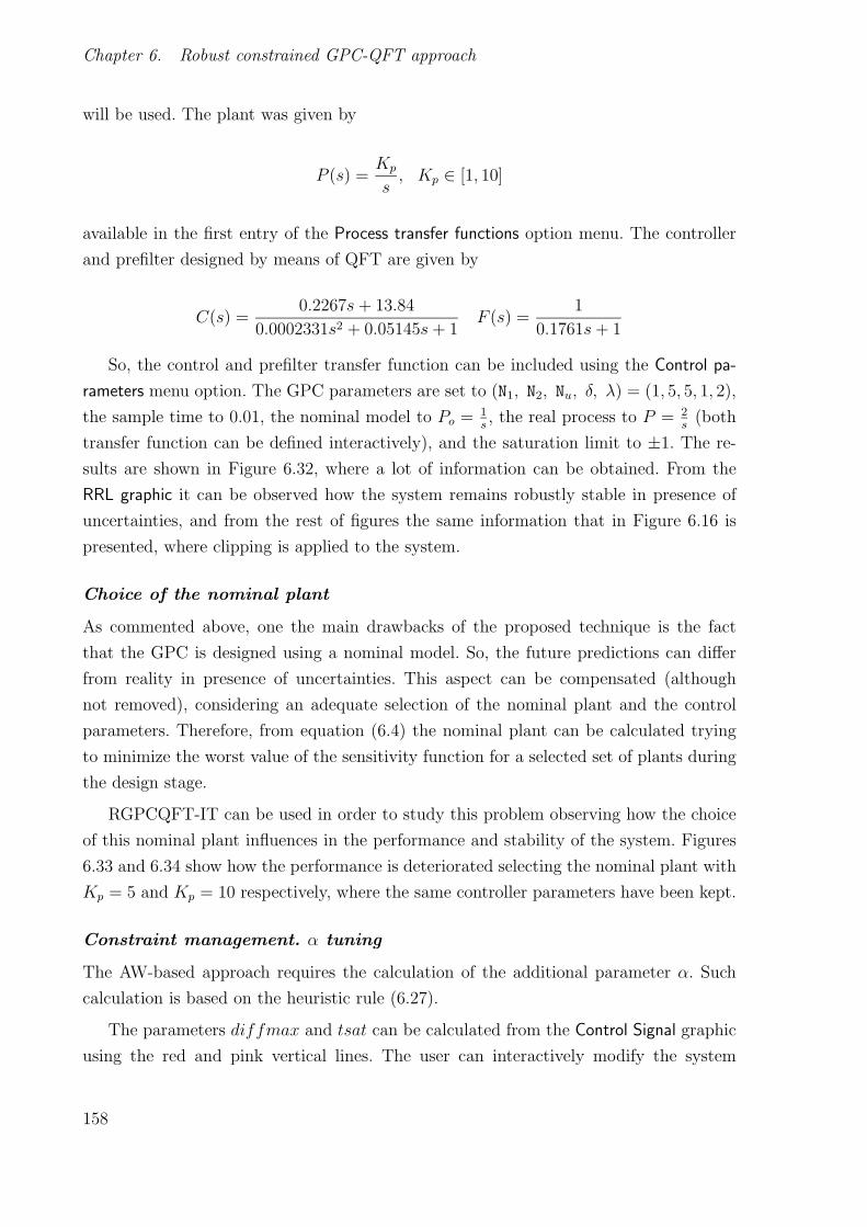
Chapter 6. Robust constrained GPC-QFT approach
will be used. The plant was given by
P (s) =Kp
s, Kp ∈ [1, 10]
available in the first entry of the Process transfer functions option menu. The controller
and prefilter designed by means of QFT are given by
C(s) =0.2267s+ 13.84
0.0002331s2 + 0.05145s+ 1F (s) =
1
0.1761s+ 1
So, the control and prefilter transfer function can be included using the Control pa-
rameters menu option. The GPC parameters are set to (N1, N2, Nu, δ, λ) = (1, 5, 5, 1, 2),
the sample time to 0.01, the nominal model to Po = 1s, the real process to P = 2
s(both
transfer function can be defined interactively), and the saturation limit to ±1. The re-
sults are shown in Figure 6.32, where a lot of information can be obtained. From the
RRL graphic it can be observed how the system remains robustly stable in presence of
uncertainties, and from the rest of figures the same information that in Figure 6.16 is
presented, where clipping is applied to the system.
Choice of the nominal plant
As commented above, one the main drawbacks of the proposed technique is the fact
that the GPC is designed using a nominal model. So, the future predictions can differ
from reality in presence of uncertainties. This aspect can be compensated (although
not removed), considering an adequate selection of the nominal plant and the control
parameters. Therefore, from equation (6.4) the nominal plant can be calculated trying
to minimize the worst value of the sensitivity function for a selected set of plants during
the design stage.
RGPCQFT-IT can be used in order to study this problem observing how the choice
of this nominal plant influences in the performance and stability of the system. Figures
6.33 and 6.34 show how the performance is deteriorated selecting the nominal plant with
Kp = 5 and Kp = 10 respectively, where the same controller parameters have been kept.
Constraint management. α tuning
The AW-based approach requires the calculation of the additional parameter α. Such
calculation is based on the heuristic rule (6.27).
The parameters diffmax and tsat can be calculated from the Control Signal graphic
using the red and pink vertical lines. The user can interactively modify the system
158
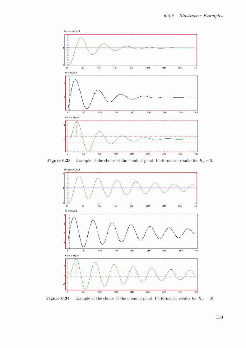
6.5.2 Illustrative Examples
Figure 6.33 Example of the choice of the nominal plant. Performance results for Kp = 5.
Figure 6.34 Example of the choice of the nominal plant. Performance results for Kp = 10.
159

Chapter 6. Robust constrained GPC-QFT approach
Figure 6.35 Calculation of diffmax and tsat parameters for AW-based approach.
Figure 6.36 RGPCQFT-IT. AW-based approach for α = 220.1.
uncertainty in order to obtain their correct values. Figure 6.35 shows that the maximum
values for the example (using a nominal plant with Kp = 1) are obtained for the plant
with Kp = 1 where diffmax = 1.42 and tsat = 1.55. Therefore, the initial value for α is
given by α = 1.550.01
· 2.42 = 220.1. Figure 6.36 shows the results for this value.
160

6.6 Conclusions about GPC-QFT approach
Figure 6.37 RGPCQFT-IT. α effect on AW-based approach.
The study of the influence of α parameter can also be performed using RGPCQFT-
IT. Figure 6.37 shows an example where a sweep in α is performed using the associated
option from the Settings menu. The α parameter is set to α = 5, 200, 1000, observing
that the systems leaves the saturation as fast as α is smaller but at expense of larger
changes in the reference and in the control signals.
6.6 Conclusions about GPC-QFT approach
A mixed GPC-QFT approach has been presented in this chapter constituting one of the
main contributions of the thesis. The aim is to design a predictive control algorithm aug-
menting the robustness in presence of uncertainties. From the obtained results, it can be
observed that the proposed approach presents bidirectional advantages. It is possible to
control an uncertain plant using a nominal GPC in such a way that the control system
is slightly affected by the residual uncertainty. Furthermore, the prediction capability,
the control and tracking weighting factors, and the input constraints management can
be included in QFT in an easy way. On the other hand, the system has been stud-
161
Chapter 6. Robust constrained GPC-QFT approach
ied to face disturbance rejection. Some of the approaches presented for the constraint
management showed feasibility problems, being the AW-based and worst case identifi-
cation approaches those which respond correctly in presence of disturbances. For these
approaches the system rejects the disturbances even the inner loop having steady state
error. The algorithm, in spite of lacking of a rigorous development to guarantee robust
stability, presents a high computational efficiency and an easy implementation, where
this has been demonstrated with the development of RGPCQFT-IT. The use of transfer
function formulation with uncertain parameters has a great acceptance in the industrial
environment, but it presents a great limitation in order to formalize the results. If the
problem is globally treated considering the presence of the non-linear element (for in-
stance, using approximations with conic sectors in the cases with symmetric saturation
and centered at the origin), the algorithm would try to avoid the system goes into sat-
uration, since probably strong penalizations would be set to prevent the loop is broken
due to the saturation.
As disadvantages of the proposed technique, the main one is the fact that the GPC is
designed using a nominal model. So, the future predictions can differ from the reality in
presence of uncertainties, specially when the system is in saturation. This aspect can be
compensated (although not removed), considering an adequate selection of the nominal
plant and the control parameters. Other disadvantage associated to this technique is its
engineering character, involving QFT design, where a finite set of plants is selected to
work.
162

7
GPC-QFT approach using LinearMatrix Inequalities
As commented in other chapters, there is a need for looking for computationally afford-
able robust predictive control algorithms that are suitable for on-line implementation.
In chapter 6, a mixed GPC-QFT approach has been proposed obtaining good compu-
tational efficiency and promising simulation results. However, the algorithm lacks of a
rigorous theoretical study to guarantee robust stability. The use of transfer function
formulation with uncertain parameters has a great acceptance in the industrial environ-
ment, but it is difficult to formalize the results in presence of constraints (for example,
to ensure constrained robust stability). Linear Matrix Inequalities (LMI)[22] have been
proposed by several authors as solution to solve constrained robust predictive control
algorithms in polynomial time using state space representations [98], where constrained
robust stability can explicitly be ensured.
Thus, a possible solution to prove robust stability in the GPC-QFT approach when
constraints are active, could be to translate the problem into a state space representation,
and then using LMI to obtain a state-vector feedback in such a way that the input
reference to the inner loop is calculated in order to satisfy robust tracking problems
considering input saturation (see Figure 7.1). This chapter describes the different steps
necessary to obtain such solution and how the problem with input saturation in the inner
loop can be solved using LMI-based solutions [2].
Figure 7.1 Control system scheme for LMI-based approach
163
Chapter 7. GPC-QFT approach using Linear Matrix Inequalities
The results presented in this chapter have been obtained under an strong collabora-
tion with Dr. Teodoro Alamo Cantarero from the University of Seville, Spain.
7.1 State space representation of the inner loop.
As commented above, it is necessary to obtain the state space representation for the
inner loop in the GPC-QFT approach in order to apply LMI-based solutions. GPC is
based on CARIMA model, where the following plant representation is considered
A(z−1)y(t) = z−dB(z−1)u(t− 1)
where d represents the time delay. Since this parameter can be included into the B(z−1)
polynomial, the plant can be described by
A(z−1)y(t) = B(z−1)u(t− 1) (7.1)
being
A(z−1) =n∏i=1
(1 + piz−1), B(z−1) = Kz
m∏i=1
(1 + ciz−1) (7.2)
The plant parametersKz, c1, . . . , cm, p1, . . . , pn are considered uncertain and supposed
to lie within known intervals due to the presence of uncertainties in the plant time domain
parameters (see 2.6). That is,
Kz ∈ [Kz,min, Kz,max]
ci ∈ [ci,min, ci,max], i = 1, . . . ,m
pi ∈ [pi,min, pi,max], i = 1, . . . , n
The polynomials A(z−1) and B(z−1) can be rewritten as
A(z−1) = 1 + a1z−1 + a2z
−1 + . . .+ anz−n (7.3)
164

7.1 State space representation of the inner loop.
B(z−1) = b0 + b1z−1 + b2z
−1 + . . .+ bmz−m (7.4)
where the coefficients a1, . . . , an, b0, . . . , bm, depend multilineally on the parametric vector
φ = [Kz, c1, . . . , cm, p1, . . . , pn]T . That is, each coefficient depends affinely on each element
of vector φ. In order to express explicitly the dependence on the vector φ, the coefficients
can be expressed as b0(φ), . . . , bm(φ), a1(φ), . . . , an(φ).
Considering the plant dynamics (7.1) and the polynomials A(z−1) and B(z−1), it
results that
y(t) = −n∑i=1
ai(φ)y(t− i) +m∑i=0
bi(φ)u(t− i− 1) (7.5)
or
y(t+ 1) = −n∑i=1
ai(φ)y(t− i+ 1) +m∑i=0
bi(φ)u(t− i) (7.6)
The plant dynamics can be represented by a state-space representation, where the pro-
posed state depends on the current output, and the past outputs and inputs in the
following way
xp(t) = [y(t) y(t− 1) . . . y(t− n+ 1) u(t− 1) . . . u(t−m)]T (7.7)
This state selection has the advantage that the state xp(t) is always accessible, that
is, the value of xp(t) is known since it is always possible to access to the output y(t) and
input u(t) signals. So, the state space representation is given by
xp(t+1) =
⎡⎢⎢⎢⎢⎢⎢⎢⎢⎢⎢⎢⎢⎢⎢⎢⎢⎢⎢⎢⎢⎢⎢⎢⎢⎢⎣
−a1 −a2 . . . −an−1 −an b1 b2 . . . bm−1 bm
1 0 . . . 0 0 0 0 . . . 0 0
0 1 . . . 0 0 0 0 . . . 0 0...
.... . .
......
......
. . ....
...
0 0 . . . 1 0 0 0 . . . 0 0
0 0 . . . 0 0 0 0 . . . 0 0
0 0 . . . 0 0 1 0 . . . 0 0
0 0 . . . 0 0 0 1 . . . 0 0...
.... . .
......
......
. . ....
...
0 0 . . . 0 0 0 0 . . . 1 0
⎤⎥⎥⎥⎥⎥⎥⎥⎥⎥⎥⎥⎥⎥⎥⎥⎥⎥⎥⎥⎥⎥⎥⎥⎥⎥⎦
xp(t)+
⎡⎢⎢⎢⎢⎢⎢⎢⎢⎢⎢⎢⎢⎢⎢⎢⎢⎢⎢⎢⎢⎢⎢⎢⎢⎢⎣
b0
0...
0
0
1
0
0...
0
⎤⎥⎥⎥⎥⎥⎥⎥⎥⎥⎥⎥⎥⎥⎥⎥⎥⎥⎥⎥⎥⎥⎥⎥⎥⎥⎦
u(t)
(7.8)
165

Chapter 7. GPC-QFT approach using Linear Matrix Inequalities
y(t) =[
1 0 0 . . . 0]xp(t) (7.9)
Considering that the coefficients a1, . . . , an, b0, . . . , bm depend on the parametric vector
φ, the system dynamics can be rewritten as
x+p = Ap(φ)xp +Bp(φ)u (7.10)
y = Cpxp (7.11)
where xp denotes the state vector, u the system input, and x+p the next state for the
state xp (xp(t+ 1)).
The plant disturbances have not been included along the previous description. Bounded
disturbances in the plant represented by the CARIMA model
A(z−1)y(t) = B(z−1)u(t− 1) + T (z−1)ε(t)
∆(7.12)
where ∆ = 1− z−1. It is assumed that the coefficients of the T (z−1) polynomial depends
multilineally on a bounded parametric vector φT and ε(t) is bounded for all t > 0, that
is, ‖ε(t)‖∞ < εmax, ∀t.
Following the same steps as previously, the system dynamics can be rewritten as
x+p = Ap(φ)xp +Bp(φ)u+ Ep(φ) (7.13)
y = Cpxp
In this representation, φ is a parametric vector containing φ, φT and ε. Furthermore,
it can be assumed that φ can only take values within a convex set (typically an hyperrect-
angle). Finally, notice that Ap(φ), Bp(φ) and Ep(φ) depends multilineally on parametric
vector φ.
7.1.1 Controller and prefilter representation.
Assume available state space descriptions for the prefilter F (z−1) and controller C(z−1).
Denoting xF as the state vector of the filter F (z−1), r the filter input and rF the filter
output, it is supposed that matrixes AF , BF , CF , and DF describe the filter dynamics
166

7.1.2 Inner loop representation. QFT loop.
as follows
x+F = AFxF +BF r (7.14)
rF = CFxF +DF r
In the same way, xC denotes the state vector for the controller C(z−1) and u the
controller output. The matrices AC , BC , CC and DC describe the controller dynamics as
follows
x+C = ACxC +BC(rF − y) (7.15)
u = CCxC +DC(rF − y)
Note that the input to the controller is given by the filter output rF minus the plant
output y, and the plant is subject to uncertainties and disturbances as discussed above.
7.1.2 Inner loop representation. QFT loop.
As commented previously, the goal is to design a robust predictive controller considering
input saturation in the inner loop. Therefore, the state space representation of the inner
loop must be developed including the saturation.
The input saturation in the inner loop is given by
σp(u) =
⎧⎪⎪⎪⎨⎪⎪⎪⎩
Umin if u < Umin
u if Umin ≤ u ≤ Umax
Umax if u > Umax
(7.16)
where nonsymmetric saturation can be presented.
Firstly, the saturation is redefined in order to use a symmetric representation to
facilitate the calculation. Therefore, the saturation is obtained as
σp(u) = Lsσ(1
Ls(u− uc)) + uc (7.17)
167
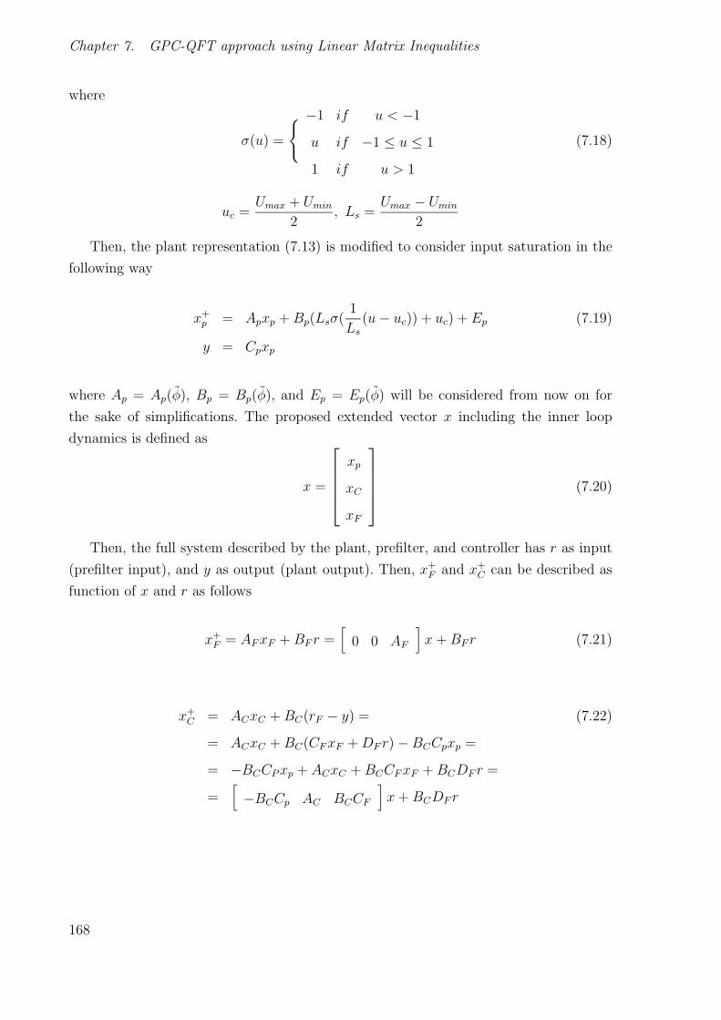
Chapter 7. GPC-QFT approach using Linear Matrix Inequalities
where
σ(u) =
−1 if u < −1
u if −1 ≤ u ≤ 1
1 if u > 1
(7.18)
uc =Umax + Umin
2, Ls =
Umax − Umin2
Then, the plant representation (7.13) is modified to consider input saturation in the
following way
x+p = Apxp +Bp(Lsσ(
1
Ls(u− uc)) + uc) + Ep (7.19)
y = Cpxp
where Ap = Ap(φ), Bp = Bp(φ), and Ep = Ep(φ) will be considered from now on for
the sake of simplifications. The proposed extended vector x including the inner loop
dynamics is defined as
x =
⎡⎢⎢⎢⎣xp
xC
xF
⎤⎥⎥⎥⎦ (7.20)
Then, the full system described by the plant, prefilter, and controller has r as input
(prefilter input), and y as output (plant output). Then, x+F and x+
C can be described as
function of x and r as follows
x+F = AFxF +BF r =
[0 0 AF
]x+BF r (7.21)
x+C = ACxC +BC(rF − y) = (7.22)
= ACxC +BC(CFxF +DF r) −BCCpxp =
= −BCCPxp + ACxC +BCCFxF +BCDF r =
=[−BCCp AC BCCF
]x+BCDF r
168

7.1.2 Inner loop representation. QFT loop.
being the control signal u obtained in the following way
u = CCxC +DC(rF − y) = (7.23)
= CCxC +DC(CFxF +DF r) −DCCpxp =
= −DCCpxp + CCxC +DCCFxF +DCDF r =
=[−DCCp CC DCCF
]x+DCDF r =
= Cux+Dur
In this way, using the new plant representation (7.19), and the prefilter and controller
state-space dynamics (7.21-7.22), the closed-loop state space representation for the inner
loop is described as
x+ =
[ Ap 0 0
−BCCp AC BCCF
0 0 AF
]x+
[ LsBp
0
0
]σ(CuLsx+
Dur − ucLs
)+
+
[ Ep +Bpuc
0
0
]+
[ 0
BCDF
BF
]r
or equivalently
x+ = Ax+Buσ(CuLsx+
Dur − ucLs
)+ E +Brr (7.24)
y = Cyx
where
A =
⎡⎢⎢⎢⎣
Ap 0 0
−BCCp AC BCCF
0 0 AF
⎤⎥⎥⎥⎦ , Bu =
⎡⎢⎢⎢⎣LsBp
0
0
⎤⎥⎥⎥⎦ , E =
⎡⎢⎢⎢⎣Ep +Bpuc
0
0
⎤⎥⎥⎥⎦ , Br =
⎡⎢⎢⎢⎣
0
BCDF
BF
⎤⎥⎥⎥⎦ ,
Cy =[
1 0 0]
169

Chapter 7. GPC-QFT approach using Linear Matrix Inequalities
7.2 Tracking problem. Preliminary ideas.
Most of the results obtained for constrained MPC using LMI have been proposed to
regulate the system to the origin. In this way, the results obtained in [98] can be used
to calculate a control law r = Ksx for the plant (7.24) considering the system free of
disturbances (E(φ) = 0) and regulating to the origin. Notice that x = 0 is an equilibrium
for the system and for all value of φ. Therefore, Ks can be calculated ensuring robust
stability and in such a way that the control law r = Ksx regulates to the origin for all
posible initial conditions and any value of φ [98], [22]. However, one of the objectives in
the GPC-QFT approach is to make the output y reach the reference value w. Therefore,
the problem formulation must be oriented to this objective. This chapter presents some
preliminary ideas based on the extensions proposed in [98] for set-point tracking.
Firstly, it is necessary to notice that due to the dependence on the parametric vector
φ, it is imposible to find static values for x and r (xe and re) such that the system finds
an unique equilibrium for all values of the parametric vector φ. In this work in order to
address this problem, the following control law is proposed
r = re +Ks(x− xe) (7.25)
where xe, re, and Ks will be obtained in such a way that the performance of the closed-
loop system is enhanced and the system evolution is ensured to be in an invariant ellipsoid
containing the problem initial conditions.
Substituting r in equation (7.24) by the desired control law r = re +Ks(x− xe), the
following expression is obtained
x+ = Ax+Buσ(Cux+Du(re +Ks(x− xe)) − uc
Ls
)+ E +Br(re +Ks(x− xe)) (7.26)
Then, if the change x = x − xe is considered, and so x+ = x+ − xe, the system
dynamics can be represented as
x+ = A(x+ xe) +Buσ((Cu +DuKs)x+ Cuxe +Dure − uc
Ls
)+ E +Br(re +Ksx) − xe
y = Cyx = Cyx+ Cyxe
170

7.2.1 Linear Difference Inclusion of the saturation function
Finally, if the following changes are performed
Ku = Cu +DuKs, du = Cuxe +Dure − uc
it is obtained that
x+ = ABcx+BBcσ(Kux+ du
Ls) + EBc (7.27)
y = Cyx+ Cyxe
where
ABc = (A+BrKs), BBc = Bu, EBc = E + Axe +Brre − xe
Define ℘(Ps, ρ) = xTPsx ≤ ρ as an ellipsoid where x0 ∈ ℘(Ps, ρ) with x0 = x0 − xe.
In this way, the tracking problem ensuring constrained robust stability for the system
(7.27) will be solved using LMI and performing the following objectives:
1. Firstly, the decision variables xe, re, Ks, Ps, and ρ are calculated in such a way
that the ellipsoid ℘(Ps, ρ) is invariant containing the system initial conditions x0
and using the control law r = re +Ks(x− xe).
2. After that, new constrains will be included in order to fulfill a certain performance
criteria.
These objectives will be addressed in next sections, but how to take into account the
saturation term presented in (7.27) will be addressed before.
7.2.1 Linear Difference Inclusion of the saturation function
Notice that due to the input saturation, a nonlinear term appears in the system dynam-
ics, σ(Kux+du
Ls). This nonlinear term can be approximated using the Lineal Difference
Inclusion (LDI) results obtained in [84] and [44] where it is shown that, if b ∈ R satisfies
|b| ≤ 1 then
σ(a) ∈ Coa, b, ∀a ∈ R
being Co the convex hull. In particular, if |Hsx+ h| ≤ 1 ∀x ∈ ℘(Ps, ρ) then
σ(Kux+ du
Ls) ∈ CoKux+ du
Ls, Hsx+ h, ∀(
Kux+ duLs
) ∈ R, ∀x ∈ ℘(Ps, ρ)
171

Chapter 7. GPC-QFT approach using Linear Matrix Inequalities
Therefore, each objective commented above will be translated to analyze if it satisfies
the extremes of the convex hull
x+ = ABcx+BBc(Kux+ du
Ls) + EBc (7.28)
x+ = ABcx+BBc(Hsx+ h) + EBc (7.29)
as will be shown in next sections.
On the other hand, the inequality |Hsx+ h| ≤ 1 must be considered. This inequality
can be translated to a LMI in order to be included in the final optimization problem.
The inequality can be expressed as two inequalities in the following way
Hsx+ h ≤ 1 ⇒ Hsx ≤ 1 − h, ∀x ∈ ℘(Ps, ρ) (7.30)
Hsx+ h ≥ −1 ⇒ Hsx ≥ −1 − h, ∀x ∈ ℘(Ps, ρ) (7.31)
where these inequalities must be satisfied in the ellipsoid ℘(Ps, ρ). In the next section,
this ellipsoid will be forced to be invariant containing the system initial conditions.
Considering the first inequality (7.30) and using the S− procedure (see section A.1),
it is equivalent to study the existence of λ2 ≥ 0 such that (Farkas lemma [22])
Hsx+ h+ λ2(ρ− xTPsx) ≤ 1, ∀x (7.32)
This can be expressed as
⎡⎣ 1
−x
⎤⎦T
⎡⎣ λ2ρ+ h− 1 −1
2Hs
−12HTs −λ2Ps
⎤⎦⎡⎣ 1
−x
⎤⎦ ≤ 0, ∀x (7.33)
or equivalently ⎡⎣ 1 − h− λ2ρ
12Hs
12HTs λ2Ps
⎤⎦ > 0 (7.34)
Then, pre- and post-multiplying by diag[I 2P−1s ] and making W = P−1
s , V = HsW , it
172

7.3 Robust invariant ellipsoid
results ⎡⎣ 1 − h− λ2ρ V
V T 4λ2W
⎤⎦ > 0 (7.35)
The same procedure can be applied for the second inequality (7.31) obtaining
⎡⎣ 1 + h− λ2ρ V
V T 4λ2W
⎤⎦ > 0 (7.36)
For a fixed value of λ2, notice that the obtained matrix inequalities are LMI in the
decision variables ρ, Ps, Hs, and h. The procedure to find correct values for λ2 will
be described later. As consequence of the previous results, the following property is
proposed:
Property 7.1
Suppose that there exits λ2 ≥ 0 such that LMI (7.35) and (7.36) are fulfilled, then:
σ(Kux+ du
Ls) ∈ CoKux+ du
Ls, Hsx+ h, ∀x ∈ ℘(Ps, ρ),
where P = W−1 and H = W−1V .
7.3 Robust invariant ellipsoid
As commented previously, one of the objectives is to calculate the decision variables xe,
re, Ks, Ps, and ρ in such a way that the ellipsoid ℘(Ps, ρ) is invariant including the
system initial conditions and using the control law r = re + Ks(x − xe). Therefore, in
order to ensure the ellipsoid being invariant the following inequality must be fulfilled
(x+)TPs(x+) ≤ ρ, ∀x ∈ ℘(Ps, ρ) (7.37)
173
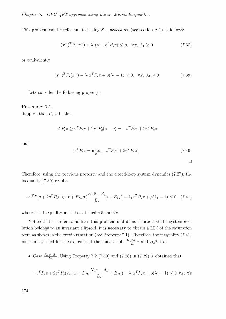
Chapter 7. GPC-QFT approach using Linear Matrix Inequalities
This problem can be reformulated using S − procedure (see section A.1) as follows:
(x+)TPs(x+) + λ1(ρ− xTPsx) ≤ ρ, ∀x, λ1 ≥ 0 (7.38)
or equivalently
(x+)TPs(x+) − λ1x
TPsx+ ρ(λ1 − 1) ≤ 0, ∀x, λ1 ≥ 0 (7.39)
Lets consider the following property:
Property 7.2
Suppose that Ps > 0, then
zTPsz ≥ vTPsv + 2vTPs(z − v) = −vTPsv + 2vTPsz
and
zTPsz = maxv
−vTPsv + 2vTPsz (7.40)
Therefore, using the previous property and the closed-loop system dynamics (7.27), the
inequality (7.39) results
−vTPsv + 2vTPs(ABcx+BBcσ(Kux+ du
Ls) + EBc) − λ1x
TPsx+ ρ(λ1 − 1) ≤ 0 (7.41)
where this inequality must be satisfied ∀x and ∀v.Notice that in order to address this problem and demonstrate that the system evo-
lution belongs to an invariant ellipsoid, it is necessary to obtain a LDI of the saturation
term as shown in the previous section (see Property 7.1). Therefore, the inequality (7.41)
must be satisfied for the extremes of the convex hull, Kux+du
Lsand Hsx+ h:
• Case Kux+du
Ls. Using Property 7.2 (7.40) and (7.28) in (7.39) is obtained that
−vTPsv + 2vTPs(ABcx+BBcKux+ du
Ls+EBc) − λ1x
TPsx+ ρ(λ1 − 1) ≤ 0,∀x, ∀v
174

7.3 Robust invariant ellipsoid
The matrix representation of the previous inequality is given by
⎡⎢⎢⎢⎣
1
x
−v
⎤⎥⎥⎥⎦T ⎡⎢⎢⎢⎣
ρ(λ1 − 1) ∗ ∗0 −λ1Ps ∗
−Ps(EBc +BLBcdu) −Ps(ABc +BLBcKu) −Ps
⎤⎥⎥⎥⎦⎡⎢⎢⎢⎣
1
x
−v
⎤⎥⎥⎥⎦ ≤ 0,∀x, ∀v
(7.42)
where BLBc = 1LsBBc and ∗ represents the transpose of the symmetric term. So,
⎡⎢⎢⎢⎣
ρ(1 − λ1) ∗ ∗0 λ1Ps ∗
Ps(EBc +BLBcdu) Ps(ABc +BLBcKu) Ps
⎤⎥⎥⎥⎦ > 0 (7.43)
Pre- and post-multiplying by diag[I P−1s P−1
s ] and making W = P−1s
⎡⎢⎢⎢⎣
ρ(1 − λ1) ∗ ∗0 λ1W ∗
(EBc +BLBcdu) (ABc +BLBcKu)W W
⎤⎥⎥⎥⎦ > 0 (7.44)
Considering that EBc = E + Axe + Brre − xe, BLBc = 1LsBBc = 1
LsBu and du =
Cuxe +Dure − uc, it results that
EBc +BLBcdu = E + Axe +Brre − xe +1
LsBu (Cuxe +Dure − uc)
= (A− I + (1
Ls)BuCu)xe + (Br + (
1
Ls)BuDu)re + E − (
1
Ls)Buuc =
Axexe +Brere + Ee
where Axe = A − I + ( 1Ls
)BuCu, Bre = Br + ( 1Ls
)BuDu and Ee = E − ( 1Ls
)Buuc.
On the other hand, reminding that ABc = A + BrKs and Ku = Cu + DuKs, it is
obtained that
ABcW +BLBcKuW = (A+BrKs)W +1
LsBu(Cu +DuKs)W =
175

Chapter 7. GPC-QFT approach using Linear Matrix Inequalities
= (A+1
LsBuCu))W + (Br +
1
LsBuDu)KsW = AwW +ByY
where Aw = A+ 1LsBuCu, By = Br + 1
LsBuDu, and Y = KsW .
Therefore, the final LMI results as follows
⎡⎢⎢⎢⎣
ρ(1 − λ1) ∗ ∗0 λ1W ∗
Axexe +Brere + Ee AwW +ByY W
⎤⎥⎥⎥⎦ > 0 (7.45)
• Case Hsx+h. In order to solve the case for Hsx+h, it is easy to see that the same
previous LMI is obtained only substituting Ku by Hs, du by h, and BLBc by BBc
⎡⎢⎢⎢⎣
ρ(1 − λ1) ∗ ∗0 λ1W ∗
(EBc +BBch) (ABc +BBcHs)W W
⎤⎥⎥⎥⎦ > 0 (7.46)
Then, knowing that EBc = E +Axe +Brre − xe, BBc = Bu and ABc = A+BrKs:
EBc +BBch = E + Axe +Brre − xe +Buh = Anlxexe +Bnlrere +Bhh+ Enle
(ABc +BBcHs)W = AW +BrKsW +BuHsW = AnlWW +BnlY Y +BvV
where Anlxe = (A − I), Bnlre = Br, Bh = Bu, Enle = E, AnlW = A, BnlY = Br,
Bv = Bu, Y = KsW , and V = HsW .
So, the resulting LMI is
⎡⎢⎢⎢⎣
ρ(1 − λ1) ∗ ∗0 λ1W ∗
Anlxexe +Bnlrere +Bhh+ Enle AnlWW +BnlY Y +BvV W
⎤⎥⎥⎥⎦ > 0 (7.47)
For a fixed value of λ1, notice that the obtained matrix inequalities are LMI in the
decision variables xe, re, ρ, Ps, Ks, Hs, and h. The procedure to find correct values for
λ1 will be described later.
176

7.4 Including performance inequality.
Property 7.3
Suppose that there exists λ1 ≥ 0 and λ2 ≥ 0 such that the LMI (7.35), (7.36), (7.45)
and (7.47) are fulfilled. Then, ℘(Ps, ρ) is an invariant ellipsoid using the control law
r = re +Ks(x − xe) and containing the system initial conditions, where P = W−1 and
K = W−1Y .
Remark 7.1
Notice that the previous LMI depends multilineally on the parametric vector φ ∈ Φ due
to the dependence of Ap = Ap(φ), Bp = Bp(φ), and Ep = Ep(φ). Then, properties 7.1
and 7.3 must be satisfied for all extreme plants of the hyperrectangle Φ.
7.4 Including performance inequality.
Consider the representation of system (7.27) for the instant time k
x+k = ABcxk +BBcσ(
Kuxk + duLs
) + EBc (7.48)
yk = Cyxk + Cyxe
and suppose the following equality
w = Cyxe (7.49)
For an initial condition x0 and the reference w, it is desired to calculate the system
input rk by the law rk = re + Ks(x − xe) such that the the following functional is
minimized
J =N∑k=0
(yk − w)Q(yk − w) + xTKu RuKux (7.50)
where Q > 0 and Ru > 0 are symmetric matrices positive semi-defined.
177
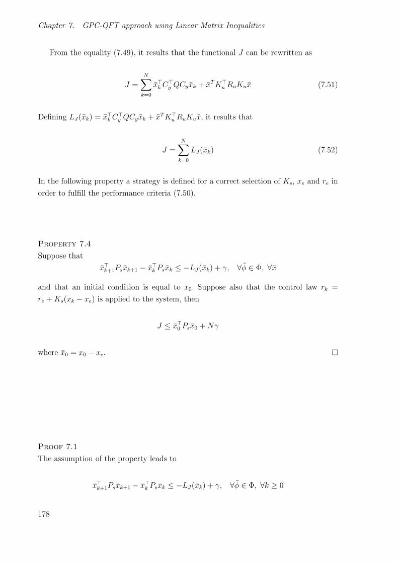
Chapter 7. GPC-QFT approach using Linear Matrix Inequalities
From the equality (7.49), it results that the functional J can be rewritten as
J =N∑k=0
xk Cy QCyxk + xTK
u RuKux (7.51)
Defining LJ(xk) = xk Cy QCyxk + xTK
u RuKux, it results that
J =N∑k=0
LJ(xk) (7.52)
In the following property a strategy is defined for a correct selection of Ks, xe and re in
order to fulfill the performance criteria (7.50).
Property 7.4
Suppose that
xk+1Psxk+1 − xk Psxk ≤ −LJ(xk) + γ, ∀φ ∈ Φ, ∀x
and that an initial condition is equal to x0. Suppose also that the control law rk =
re +Ks(xk − xe) is applied to the system, then
J ≤ x0 Psx0 +Nγ
where x0 = x0 − xe.
Proof 7.1
The assumption of the property leads to
xk+1Psxk+1 − xk Psxk ≤ −LJ(xk) + γ, ∀φ ∈ Φ, ∀k ≥ 0
178

7.4 Including performance inequality.
Therefore,
x1 Psx1 − x0 Psx0 ≤ −LJ(x0) + γ
x2 Psx2 − x1 Psx1 ≤ −LJ(x1) + γ
...
xNPsxN − xN−1PsxN−1 ≤ −LJ(xN−1) + γ
xN+1PsxN+1 − xNPsxN ≤ −LJ(xN) + γ
If the previous inequalities are added, it is obtained that
xN+1PsxN+1 − x0 Psx0 ≤ −J +Nγ
J ≤ x0 Psx0 +Nγ − xN+1PsxN+1
J ≤ x0 Psx0 +Nγ
So, from the previous property the following optimization problem can be proposed
minPs,Ks,xe,re,γ
x0 Psx0 +Nγ (7.53)
s.a. (x+)TPs(x+) − xPsx <
< −xCy QCyx− xTK
u RuKux+ γ, ∀φ ∈ Φ, ∀x
in order to calculate the control law that minimizes an upper limit of the functional.
Notice that N is a design parameter absent from problem constraints. If N is very
large, the problem solution will tend to minimize γ. The following interpretation can be
considered for γ
limN→∞
J
N≤ lim
N→∞x0 Psx0 +Nγ
N= γ (7.54)
Therefore, if N is very large the initial transitory is almost not considered (the initial
condition x0 doesn’t play a relevant role) and the emphasis is placed on improving the
future behavior. On the other hand, if N takes very small values, the initial condition
and the initial transitory gains relevance.
179

Chapter 7. GPC-QFT approach using Linear Matrix Inequalities
Then, the problem (7.53) can be reformulated as
minPs,Ks,xe,re,γ,αs
αs (7.55)
s.a. xT0 Psx0 +Nγ < αs
(x+)TPs(x+) − xTPsx < −xTCT
y QCyx− xTKTuRuKux+ γ
The problem inequalities will be translated to LMI form in order to address the
optimization problem. Firstly, the upper inequality is considered
xT0 Psx0 +Nγ < αs (7.56)
This can be easily expressed as a LMI using the Schur complement (see section A.1)
in the form ⎡⎣ αs −Nγ x(0)T
x(0) W
⎤⎦ ≥ 0 (7.57)
On the other hand, and remembering the presence of the saturation term in (7.48), the
another inequality
(x+)TPs(x+) − xTPsx < −xTCT
y QCyx− xTKTuRuKux+ γ (7.58)
must be satisfied for two extreme vertices of the LDI, Ksx+du
Lsand Hsx+ h, in the same
way that for the invariant ellipsoid. The first step consists in using Property 7.2 on the
previous inequality, where it is obtained that
−vTPsv+2vTPs(ABcx+BBcσ(Kux+ du
L)+EBc)−xTPsx < −xTCT
y QCyx−xTKTuRuKux+γ
• Case Ksx+du
Ls. Considering that x+ is described by (7.28), the previous inequality
results as
−vTPsv + 2vTPs(ABcx+ EBc) − xTPsx+ xTCTy QCyx+ xTKT
uRuKux− γ+
+2vTPsBBc(Kux+ du
Ls) ≤ 0
180

7.4 Including performance inequality.
The matrix representation is given by
⎡⎢⎢⎢⎣
1
x
−v
⎤⎥⎥⎥⎦T ⎡⎢⎢⎢⎣
−γ ∗ ∗0 −Ps + CT
y QCy +KTuRuKu ∗
−(PsEBc + PsBLBcdu) −(PsABc + PsBLBcKu) −Ps
⎤⎥⎥⎥⎦⎡⎢⎢⎢⎣
1
x
−v
⎤⎥⎥⎥⎦ ≤ 0
(7.59)
where BLBc = 1LsBBc, and the previous LMI must be satisfied ∀x and ∀v. Therefore,
it is obtained that
⎡⎢⎢⎢⎣
γ ∗ ∗0 Ps − CT
y QCy −KTuRuKu ∗
Ps(EBc +BLBcdu) Ps(ABc +BLBcKu) Ps
⎤⎥⎥⎥⎦ > 0 (7.60)
where pre- and post-multiplying by diag[I P−1s P−1
s ] and making W = P−1s , it is
obtained that
⎡⎢⎢⎢⎣
γ ∗ ∗0 W −WCT
y QCyW −WKTuRuKuW ∗
(EBc +BLBcdu) (ABc +BLBcKu)W W
⎤⎥⎥⎥⎦ > 0 (7.61)
From the Schur complement the LMI results as follows
⎡⎢⎢⎢⎢⎢⎢⎣
γ ∗ ∗ ∗0 W −WKT
uRuKuW ∗ ∗(EBc +BLBcdu) (ABc +BLBcKu)W W ∗
0 Q1/2CyW 0 I
⎤⎥⎥⎥⎥⎥⎥⎦ > 0 (7.62)
181

Chapter 7. GPC-QFT approach using Linear Matrix Inequalities
Using the Schur complement again, it is obtained that
⎡⎢⎢⎢⎢⎢⎢⎢⎢⎢⎣
γ ∗ ∗ ∗ ∗0 W ∗ ∗ ∗
(EBc +BLBcdu) (ABc +BLBcKu)W W ∗ ∗0 Q1/2CyW 0 I ∗0 R
1/2u KuW 0 0 I
⎤⎥⎥⎥⎥⎥⎥⎥⎥⎥⎦> 0 (7.63)
or equivalently
⎡⎢⎢⎢⎢⎢⎢⎢⎢⎢⎣
γ ∗ ∗ ∗ ∗0 W ∗ ∗ ∗
Axexe +Brere + Ee AwW +ByY W ∗ ∗0 Q1/2CyW 0 I ∗0 RWW +RY Y 0 0 I
⎤⎥⎥⎥⎥⎥⎥⎥⎥⎥⎦> 0 (7.64)
where Axe = A − I + ( 1Ls
)BuCu, Bre = Br + ( 1Ls
)BuDu, Ee = E − ( 1Ls
)Buuc,
Aw = A+ 1LsBuCu, By = Br + 1
LsBuDu, Y = KsW and
R1/2u KuW = R1/2
u (Cu +DuKs)W = R1/2u CuW +R1/2
u DuKsW = RwW +RyY.
• Case Hsx + h. In this case, it is easy to see that the same LMI (7.64) is obtained
only replacing Ku by Hs, du by h, and BLBc by BBc. So, it is obtained that
⎡⎢⎢⎢⎢⎢⎢⎢⎢⎢⎣
γ ∗ ∗ ∗ ∗0 W ∗ ∗ ∗
(EBc +BBch) (ABc +BBcHs)W W ∗ ∗0 Q1/2CyW 0 I ∗0 R
1/2u KuW 0 0 I
⎤⎥⎥⎥⎥⎥⎥⎥⎥⎥⎦> 0 (7.65)
Then, using the same notation that in previous sections where, EBc + BBch =
Anlxexe+Bnlrere+Bhh+Enle, ABc+BBcHs = AnlWW+BnlY Y +BvV , R1/2u HsW =
182

7.5 Final optimization problem
R1/2V = RvV , Y = KsW , and V = HsW , the LMI can be represented as follows
⎡⎢⎢⎢⎢⎢⎢⎢⎢⎢⎣
γ ∗ ∗ ∗ ∗0 W ∗ ∗ ∗
Anlxexe +Bnlrere +Bhh+ Enle AnlWW +BnlY Y +BvV W ∗ ∗0 Q1/2CyW 0 I ∗0 RvV 0 0 I
⎤⎥⎥⎥⎥⎥⎥⎥⎥⎥⎦> 0
(7.66)
Finally, the equality (7.49), which was supposed before, must be included in the
optimization problem. Therefore, the optimization problem has been reformulated to
minimize the value of αs subject to a set of LMI. The following section describes the
final optimization problem and the different obtained LMI.
7.5 Final optimization problem
Notice that in section 7.1.2, it was considered that Ap = Ap(φ), Bp = Bp(φ), and
Ep = Ep(φ) for simplification reasons. That is, it is necessary to remind that the matrices
of the plant depend multilineally on the parametric vector φ. In this way, the previous
LMI that were formulated for the nominal case, must be satisfied for all extreme values
of the hyperrectangle Φ. Hence, the final problem can be formulated to calculate the
decision variables xe, re, Ks, Ps, ρ, Hs, and h, in such a way that using the control
law r = re + Ks(x − xe), ℘(Ps, ρ) is an invariant ellipsoid and the system fulfills the
performance criteria given by J (7.50). The final optimization problem is given by
minPs,Ks,xe,re,γ,αs
αs (7.67)
s.a. xT0 Psx0 +Nγ < αs
(x+)TPs(x+) − xTPsx < −xTCT
y QCyx− xTKTuRuKux+ γ
Then, considering the results obtained in previous section, a conservative way to solve
the optimization problem consists in solving the following constraints
w = Cyxe (7.68)
183

Chapter 7. GPC-QFT approach using Linear Matrix Inequalities
⎡⎣ αs −Nγ x(0)T
x(0) W
⎤⎦ > 0 (7.69)
⎡⎣ ρ x(0)T
x(0) W
⎤⎦ > 0 (7.70)
⎡⎢⎢⎢⎢⎢⎢⎢⎢⎢⎣
γ ∗ ∗ ∗ ∗0 W ∗ ∗ ∗
Axe(φ)xe +Bre(φ)re + Ee(φ) Aw(φ)W +By(φ)Y W ∗ ∗0 Q1/2Cy(φ)W 0 I ∗0 RW (φ)W +RY Y 0 0 I
⎤⎥⎥⎥⎥⎥⎥⎥⎥⎥⎦> 0 (7.71)
⎡⎢⎢⎢⎣
ρ(1 − λ1) ∗ ∗0 λ1W ∗
Axe(φ)xe +Bre(φ)re + Ee(φ) Aw(φ)W +BY Y W
⎤⎥⎥⎥⎦ > 0 (7.72)
⎡⎢⎢⎢⎢⎢⎢⎢⎢⎢⎢⎢⎢⎣
γ ∗ ∗ ∗ ∗0 W ∗ ∗ ∗
Anlxe(φ)xe +Bnlre(φ)re +Bh(φ)h+
+Enle(φ)
AnlW (φ)W +BnlY Y+
+Bv(φ)VW ∗ ∗
0 Q1/2Cy(φ)W 0 I ∗0 RvV 0 0 I
⎤⎥⎥⎥⎥⎥⎥⎥⎥⎥⎥⎥⎥⎦> 0
(7.73)
184

7.5 Final optimization problem
⎡⎢⎢⎢⎣
ρ(1 − λ1) ∗ ∗0 λ1W ∗
Anlxe(φ)xe +Bnlre(φ)re +Bh(φ)h+ Enle(φ) AnlW (φ)W +BnlY Y +Bv(φ)V W
⎤⎥⎥⎥⎦ > 0
(7.74)
⎡⎣ 1 − h− λ2ρ V
V T 4λ2W
⎤⎦ ≥ 0 (7.75)
⎡⎣ 1 + h− λ2ρ V
V T 4λ2W
⎤⎦ ≥ 0 (7.76)
where it is necessary to incorporate constrains for each extreme value of the hypercube
Φ. Also, as observed from the resulting constraints, some of them are BMI (Bilineal
Matrix Inequalities) containing different bilineal terms ρ(1−λ1), λ1W , λ2ρ), and 4λ2W .
So, in order to obtain an stable MPC controller with good performance, it is necessary
to choose λ1 and λ2 in a convenient way.
Property 7.5
Suppose that there exist λ1 ≥ 0 and λ2 ≥ 0 such that the constraints (7.68), (7.69),
(7.70), (7.71), (7.72), (7.73), (7.74), (7.75), and (7.76) are feasible for every extreme of
the hypercube Φ. Then, there exits a control law r = re + Ks(x − xe) providing that
℘(Ps, ρ) is an invariant ellipsoid and the system fulfills the performance criteria given by
J (7.50), where P = W−1 and K = W−1Y .
A Branch & Bound algorithm is proposed to find the optimal solution. Before describing
the algorithm, some aspects must be considered:
• From the constraints it is easy to see that λ1 ∈ [λ1, λ1) = [0, 1) and λ2 ∈ [λ2, λ2) =
[0,∞), respectively. Notice that λi and λi represent the minimum and maximum
values for λi with i = 1, 2.
• A lower bound solution is that obtained considering that there exist λ1 ∈ [λ1, λ1)
and λ2 ∈ [λ2, λ2) such that the constraints (7.68), (7.69), (7.70), (7.71), and (7.73)
185
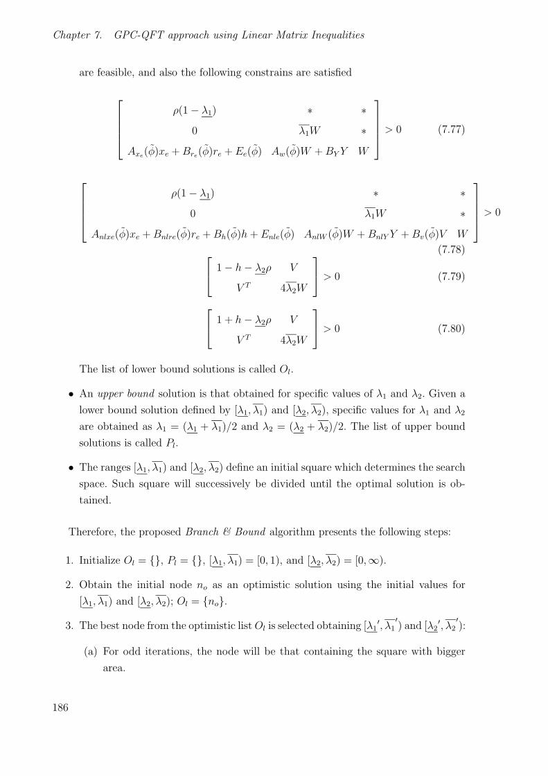
Chapter 7. GPC-QFT approach using Linear Matrix Inequalities
are feasible, and also the following constrains are satisfied
⎡⎢⎢⎢⎣
ρ(1 − λ1) ∗ ∗0 λ1W ∗
Axe(φ)xe +Bre(φ)re + Ee(φ) Aw(φ)W +BY Y W
⎤⎥⎥⎥⎦ > 0 (7.77)
⎡⎢⎢⎢⎣
ρ(1 − λ1) ∗ ∗0 λ1W ∗
Anlxe(φ)xe +Bnlre(φ)re +Bh(φ)h+ Enle(φ) AnlW (φ)W +BnlY Y +Bv(φ)V W
⎤⎥⎥⎥⎦ > 0
(7.78)⎡⎣ 1 − h− λ2ρ V
V T 4λ2W
⎤⎦ > 0 (7.79)
⎡⎣ 1 + h− λ2ρ V
V T 4λ2W
⎤⎦ > 0 (7.80)
The list of lower bound solutions is called Ol.
• An upper bound solution is that obtained for specific values of λ1 and λ2. Given a
lower bound solution defined by [λ1, λ1) and [λ2, λ2), specific values for λ1 and λ2
are obtained as λ1 = (λ1 + λ1)/2 and λ2 = (λ2 + λ2)/2. The list of upper bound
solutions is called Pl.
• The ranges [λ1, λ1) and [λ2, λ2) define an initial square which determines the search
space. Such square will successively be divided until the optimal solution is ob-
tained.
Therefore, the proposed Branch & Bound algorithm presents the following steps:
1. Initialize Ol = , Pl = , [λ1, λ1) = [0, 1), and [λ2, λ2) = [0,∞).
2. Obtain the initial node no as an optimistic solution using the initial values for
[λ1, λ1) and [λ2, λ2); Ol = no.
3. The best node from the optimistic listOl is selected obtaining [λ1′, λ1
′) and [λ2
′, λ2′):
(a) For odd iterations, the node will be that containing the square with bigger
area.
186

7.5 Final optimization problem
(b) For even iterations, the node will be that with better performance.
4. New upper bound solution is calculated using the best node calculated in the
previous step, [λ1′, λ1
′) and [λ2
′, λ2′). The solution is calculated trying to solve the
optimization problem for λ1 = λ′1m = (λ1′ +λ1
′)/2 and λ2 = λ′2m = (λ2
′ +λ2′)/2. If
the optimization problem has solution for these values of λ1 and λ2, the new value
is included in the list of pessimistic solutions Pl. Then a local search is performed
trying to improve the found solution. The local search is based on the following
heuristic steps:
(a) The values obtained for λ1 and λ2, and the obtained performance solution are
considered as initial variables.
(b) Solve the optimization problem (7.67) using λ1 and λ2 and obtaining values
for W and ρ. If a better performance solution is obtained, then the new upper
bound solution is included in the upper bound list Pl. The best performance
solution is updated with the new one.
(c) Reformulate the LMI considering λ1 and λ2 as decision variables and, W and
ρ as constant values. Solve the optimization problem obtaining new values for
λ1 and λ2.
(d) Return to step (b) while better performance solutions are obtained or until a
finite number of iterations is reached.
5. Remove worst lower bound solutions. The lower bound solutions with worst per-
formance than the best upper bound one are removed from the lower bound list
Ol.
6. New lower bound solutions are obtained. That is, four new nodes are calculated
from the node obtained in the previous step as follows
n1 = [λ1′, λ′1m], [λ2
′, λ′2m], n2 = [λ1′, λ′1m], [λ′2m, λ2
′]
n3 = [λ′1m, λ1′], [λ2
′, λ′2m], n4 = [λ′1m, λ1′], [λ′2m, λ2
′]
The lower bound solution calculated for ni, i = 1, .., 4 will be removed if the solution
is empty (the optimization problem is not feasible), the obtained performance is
worst than the best upper bound solution, or the square defined by the associated
ranges on λ1 and λ2 is too small. Otherwise, it will be included in the lower bound
list Ol.
187

Chapter 7. GPC-QFT approach using Linear Matrix Inequalities
7. Return to 3 until the optimal solution is reached or while there exist lower bound
solutions.
Notice that the convergence of the optimal solution is ensured using the previous
algorithm. This is due to that the search is not always performed looking for the best
solution, since in odd iterations the solution is chosen based on the greatest search space
of λ1 and λ2.
7.6 Numerical Examples
The integrator example presented in chapter 6 is used in order to test the proposed
optimization problem and to compare it with the other proposed approaches. The plant
was defined by
P (s) =Kp
s, Kp ∈ [1, 10]
and the prefilter and controller by
C(s) =0.2267s+ 13.84
0.0002331s2 + 0.05145s+ 1F (s) =
1
0.1761s+ 1
Considering the sample time Tm = 0.01 s, N = 20, Ru = 1, Q = 1, w = 1, and x0 =
[0 0 0 0]T , the Branch and Bound algorithm found an optimal solution for λ1 = 0.993275
and λ2 = 0.005826 obtaining
Ks =[
22.89834 −0.32026 −1.64460 −1.3475]
Figure 7.2 shows the results of applying the obtained solution to the example considering
all plants of the family. It can be seen how the system reaches the proposed reference
w = 1 obtaining good performance. Comparing the results with the approaches presented
in chapter 6, the proposed LMI-based approach presents similar results, but also ensuring
constrained robust stability. Notice that, the LMI-based approach is implemented with
low computational load where the state vector K is calculated off-line. However, the
optimization problem could be solved on-line at each instant time in order to obtain
more optimal results, where the state vector K is always calculated based on the current
state of the system. Then, in this case, the LMI-based approach would require bigger
188
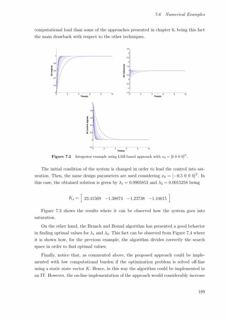
7.6 Numerical Examples
computational load than some of the approaches presented in chapter 6, being this fact
the main drawback with respect to the other techniques.
0 2 4 6 8 100
0.2
0.4
0.6
0.8
1
All
ou
tpu
ts
Time(s)0 2 4 6 8 10
−1.5
−1
−0.5
0
0.5
1
1.5
2
2.5
3
3.5
All
refe
ren
ces
Time(s)
0 2 4 6 8 10−0.2
0
0.2
0.4
0.6
0.8
1
All
con
tro
l sig
nal
s
Time(s)
Figure 7.2 Integrator example using LMI-based approach with x0 = [0 0 0 0]T .
The initial condition of the system is changed in order to lead the control into sat-
uration. Then, the same design parameters are used considering x0 = [−0.5 0 0 0]T . In
this case, the obtained solution is given by λ1 = 0.9905853 and λ2 = 0.0015258 being
Ks =[
23.41569 −1.38874 −1.23738 −1.44615]
Figure 7.3 shows the results where it can be observed how the system goes into
saturation.
On the other hand, the Branch and Bound algorithm has presented a good behavior
in finding optimal values for λ1 and λ2. This fact can be observed from Figure 7.4 where
it is shown how, for the previous example, the algorithm divides correctly the search
space in order to find optimal values.
Finally, notice that, as commented above, the proposed approach could be imple-
mented with low computational burden if the optimization problem is solved off-line
using a static state vector K. Hence, in this way the algorithm could be implemented in
an IT. However, the on-line implementation of the approach would considerably increase
189
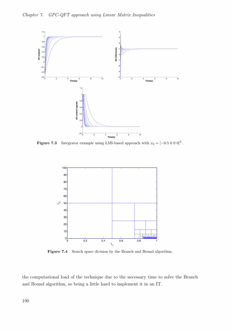
Chapter 7. GPC-QFT approach using Linear Matrix Inequalities
0 2 4 6 8 10−0.6
−0.4
−0.2
0
0.2
0.4
0.6
0.8
1
1.2
All
ou
tpu
ts
Time(s)0 2 4 6 8 10
−4
−3
−2
−1
0
1
2
3
4
All
refe
ren
ces
Time(s)
0 2 4 6 8 10−0.2
0
0.2
0.4
0.6
0.8
1
1.2
All
con
tro
l sig
nal
s
Time(s)
Figure 7.3 Integrator example using LMI-based approach with x0 = [−0.5 0 0 0]T .
0 0.2 0.4 0.6 0.8 10
10
20
30
40
50
60
70
80
90
100
λ1
λ 2
Figure 7.4 Search space division by the Branch and Bound algorithm.
the computational load of the technique due to the necessary time to solve the Branch
and Bound algorithm, so being a little hard to implement it in an IT.
190

7.7 Conclusions
7.7 Conclusions
A LMI-based approach has been proposed as solution to the lack of rigorous theoretical
development to guarantee robust stability of the algorithms proposed in chapter 6. In this
way the GPC-QFT approach has been translated to state space representation, and LMI
has been used to obtain a state-vector feedback in such a way that the input reference to
the inner loop is calculated in order to satisfy robust tracking problems considering input
saturation. The proposed solution consists in solving a set of constraints being formed
by several LMI and BMI, where a Branch and Bound algorithm has been developed in
order to solve the bilinear terms. Notice that the algorithm is implemented for tracking
problems where the aim is to regulate to a fixed reference value and not to the origin,
and also input constraints are presented in the inner loop of the system, what is not
usual in the literature.
The approach has presented similar performance results that the techniques of chap-
ter 6, but also ensuring constrained robust stability. On the other hand, the proposed
technique could be implemented in a IT with low computational burden in the off-
line implementation case. However, if the optimization problem is solved on-online, the
computational load is considerably increased, being the main drawback of the proposed
approach.
191


8
Other Interactive Tools
The acceptance of the IT developed in chapters 4 and 5 has been quite high. After two
years testing the IT related to GPC in process control courses, the students gave high
quotations to several questions posed in surveys and tests that they must fulfill when
finishing the subjects regarding the use of IT in control learning. As consequence, the
author has strongly collaborated in other works aimed at developing IT and remote labs
in different fields of control education. This chapter presents a couple of them where two
new interactive tools are described related to the greenhouse climate control and mobile
robotics fields. Firstly, a virtual lab for teaching greenhouse climatic control is presented
[69], [70]. The tool consists on a structured graphic screen allowing the access to a full
greenhouse climate model with a collection of specific controllers, in such a way that the
students can put into practice the knowledge acquired in the theoretical lessons without
space-temporal constraints. On the other hand, an interactive tool is presented aimed
at facilitating the understanding of the algorithms and techniques involved in solving
mobile robotics problems, from those modelling the mechanics of mobility to those used
in navigation, showing how the modification of a certain element of the system affects
to the other components [61], [68]. Both applications are self-contained.
8.1 Virtual Lab for Teaching Greenhouse Climatic Control
Nowadays, the agro-alimentary sector is incorporating new technologies, due to the large
production demands, and the diversity, quality, and market presentation requirements.
Thus, a technological renovation of the sector is required and the control engineering
plays a decisive role by the incorporation of automatic control and robotics techniques
in all the agricultural production levels: plantation, production, harvest, post-harvest
processes, and transportation. Therefore, introductory courses of automatic control and
robotics are being included in the modern agronomy studies. Future engineers will have
to use, understand, and implement the new advances in automation in the sector. This
193

Chapter 8. Other Interactive Tools
section presents a tool which helps to perform this task in the greenhouse climatic control
topic. As commented in previous chapters, a development of a great number of projects
and research works for improving the education in the Automatic Control field has been
carried out during the last years [41]. There are many works about interactivity, web-
based simulation, and virtual and remote labs ([40], [58], [110], [144]), that open a wide
range of possibilities as support to the students’ education. Some of these works, such
as remote labs [60] and virtual courses [135], are being used for teaching greenhouse
climatic control, in undergraduate and doctorate courses. In order to complement the
previous works and advance in this field, a virtual lab for teaching greenhouse climatic
control [69], [70] is presented in this section. This tool has been developed using Easy
Java Simulation [43] and the research results obtained by [137] regarding greenhouse
modelling and climatic control. This virtual lab permits the students to put into practice
their knowledge from any place connected to Internet and without timetable constraints.
A full greenhouse climatic control course composed of three elements is now available:
the theoretical lessons can be learned using a virtual course [135], then they can be put
into practice using the virtual lab presented in this section and, finally, real tests can be
performed remotely using a greenhouse scale model [60].
8.1.1 Greenhouse climate model
A greenhouse climate model is necessary in order to simulate the climate behavior in a
greenhouse and testing the control algorithms. The model was developed in [137], where
the time-evolution of the state variables characterizing the greenhouse air volume and
the surfaces delimiting this volume was represented by a system of differential equations
which can be expressed, in a general form, as
dX
dt= f(X,U,D, V, C, t) with X(ti) = Xi (8.1)
whereX = X(t) is a n-dimensional vector of state variables, U = U(t) is am-dimensional
vector of input variables, D = D(t) is an o-dimensional vector of disturbances, V = V (t)
is a p-dimensional vector of the system variables, C is a q-dimensional vector of system
constants, t is the time, Xi is the known state at the initial time ti, and f = f(t) is a
nonlinear function based on mass and heat transfer balances.
The number of equations describing the system and their characteristics depend on
the greenhouse elements, the control actuators, and the cropping system, so that the
model has been developed assuming the following hypotheses:
• The greenhouse was considered to be integrated by six elements: the cover, the
194

8.1.1 Greenhouse climate model
inside air, the crop, the soil surface, and two soil sub-layers.
• The main state variables of the model are the inside air temperature and humid-
ity (expressed as absolute humidity), cover temperature, soil surface temperature,
intermediate soil layer temperature, and PAR radiation.
• The exogenous and disturbance inputs acting on the system are the outside air
temperature and absolute humidity, wind speed and direction, sky temperature,
outside global solar radiation, and the intensity of greenhouse whitening.
• The control inputs of the system are the open area, or aperture angle of the vents,
the position of the shading screen (on/off), and the water temperature of the
heating pipe system.
• The modules allowing the calculation of the temperature variables are based on
the heat transfer balance of surfaces or volumes, where the following physical pro-
cesses are included: absorption of solar and long wave radiation, heat transfer
by convection and conduction, and latent heat exchanges (crop transpiration, soil
evaporation, and condensation). The module calculating the internal air humid-
ity is based on the water vapour balance of the greenhouse volume. It includes
the exchanges between the inside and the outside air, and the condensation and
evapotranspiration processes.
The model implementation was performed using a process-oriented method. The
model was hierarchically structured, using a top-down approach from the upper level,
including the main modules, to the lower level, where each specific process is formulated
and quantified [137]. The following five hierarchical levels were defined in the model:
1. System level. It consists on the model main block (supervisor), in which are defined
the inputs (control and disturbances) and outputs, as well as the links and feedback
between the different modules.
2. Variable-type level, corresponding to the three main classes of climate variables
(radiation, temperature, and humidity).
3. Variable level, including all the state variables related to a given class (e.g., the
temperature level is divided into four sub-levels: cover, soil surface, soil layer, and
greenhouse air temperatures).
4. Process level, integrating the modules aimed to describe the physical and physio-
logical processes involved in the state-variable modules.
195

Chapter 8. Other Interactive Tools
5. Implementation level, corresponding to the code that implements a process of the
previous upper level.
8.1.2 Greenhouse Climatic Control
Crop production in a greenhouse is affected by the inside climate, and therefore, it is
necessary to keep the main variables within a specific range. The variables used in the
control problem are shown in Figure 8.1: controlled variables (PAR radiation, inside
temperature, and relative humidity), manipulated variables (common actuators such
as natural ventilation, shade screen, and heating), and disturbance variables (outside
climate, the crop, and other greenhouse elements such as the cover and the soil).
Figure 8.1 Climatic control variables.
Temperature control problem
Temperature is the main climatic variable affecting the crop growth, and thus, this
variable has been traditionally controlled in the greenhouses. The plants require usually
the daylight and high temperature to correctly perform the photosynthesis and growth.
However, it is not necessary to keep high temperatures during the night, because the crop
is inactive. In order to control the temperature, usually the ventilation is used during
the day and heating during the night. Therefore, there are two set-points: the ventilation
set-point and the heating set-point ([138], [134]). So, it is possible to define five periods
during the day with different set-points (see Figure 8.2), some of which does not require
the use of control actuators.
Temperature control using natural vents. The use of natural ventilation produces
an exchange between inside and outside air, usually in the greenhouse decreasing the
196

8.1.2 Greenhouse Climatic Control
Figure 8.2 Temperature set-point periods.
inside temperature. The controller must calculate the necessary vents opening to reach
the desired set-point. The most common controller used is a gain scheduling PI scheme
where the controller values are changed based on some disturbances: outside temperature
and wind speed. The basis of this technique will be treated in next sections.
Temperature control with heating. The heating system consists of several steel pipes
distributed along the greenhouse (Figure 8.3). These pipes are heated by hot water
circulating though them, transmitting heat to the air by convection. This physical phe-
nomenon produces an increase in the greenhouse inside temperature. Then, the control
problem consists of calculating the required temperature of the water within the pipes to
let the inside temperature reaching the desired value. In order to perform this task, the
system has one three way valve to mix the water of the boiler (constant temperature)
with the water returning from the greenhouse in a cascade structure.
The actuators have constraints as the water temperature through the pipes is lower
than the water temperature in the boiler. A classical anti-windup [5] scheme is used
to take into account this problem and avoid integrator windup. The pipes temperature
cannot be bigger than that of the boiler, but either smaller than the greenhouse inside
temperature (changeable lower saturation).
Humidity control
Water vapour inside the greenhouse is not one of the most important variables affect-
ing the crop growth. However, the humidity control has a special interest, because high
humidity may produce the appearance of diseases and decrease the transpiration, and
low humidity may cause hydric stress, closing the stomata, and reducing the photosyn-
thesis. Therefore, it is necessary to keep the humidity within a certain range. There are
197

Chapter 8. Other Interactive Tools
Figure 8.3 Greenhouse heating system and control.
two problems involved in the humidity control: the greenhouse inside temperature and
the relative humidity are inversely correlated (when one of them increases the other one
decreases and vice versa), and for controlling temperature and humidity the same ac-
tuators are used. The temperature control has the main priority because it affects to
the crop growth directly. In order to keep the humidity within a determined range, the
temperature set-point can be changed based on the inside relative humidity value.
Radiation control
The most widely used method to control the solar radiation is based on shade screens to
reduce the incoming radiation onto the crop and the soil, causing two effects: reducing
PAR radiation and slowing the crop growth due to the decrease of the photosynthesis
activities. The shade screen is always completely opened or closed to obtain a uniform
crop growth by on/off control with dead zone to avoid frequent changes in the actuators.
8.1.3 Virtual lab description
As commented before, the main aim of the tool is to facilitate the study and under-
standing of the issues involved in modeling and climatic control of greenhouses. The
tool consists of a graphic screen connected to the algorithms and a model implemented
in Matlab/Simulink [137]. In a previous exercise this model is used by the students to
understand the process dynamics in order to obtain the model parameters. In this way
they can design the controllers and test them in the virtual lab. The environment EJS
198
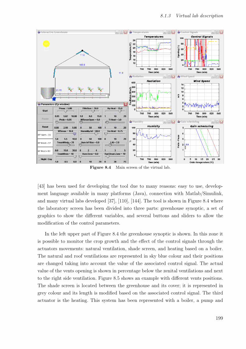
8.1.3 Virtual lab description
Figure 8.4 Main screen of the virtual lab.
[43] has been used for developing the tool due to many reasons: easy to use, develop-
ment language available in many platforms (Java), connection with Matlab/Simulink,
and many virtual labs developed [37], [110], [144]. The tool is shown in Figure 8.4 where
the laboratory screen has been divided into three parts: greenhouse synoptic, a set of
graphics to show the different variables, and several buttons and sliders to allow the
modification of the control parameters.
In the left upper part of Figure 8.4 the greenhouse synoptic is shown. In this zone it
is possible to monitor the crop growth and the effect of the control signals through the
actuators movements: natural ventilation, shade screen, and heating based on a boiler.
The natural and roof ventilations are represented in sky blue colour and their positions
are changed taking into account the value of the associated control signal. The actual
value of the vents opening is shown in percentage below the zenital ventilations and next
to the right side ventilation. Figure 8.5 shows an example with different vents positions.
The shade screen is located between the greenhouse and its cover; it is represented in
grey colour and its length is modified based on the associated control signal. The third
actuator is the heating. This system has been represented with a boiler, a pump and
199

Chapter 8. Other Interactive Tools
several pipes (Figures 8.3 and 8.4). A colour code is used: pump off/on - blue/green;
pipes off/on - grey/based on their temperature. The value of the pipes temperature is
shown next to the boiler, as it can be seen in Figure 8.6, where an example of the heating
is shown. The crop growth is considered as a disturbance for the system being possible
to modify this parameter in the graphic screen. Several plants are shown in the synoptic
and their size is changed based on the value of this disturbance.
(a) Vents and screens closed. (b) Vents and screens open.Figure 8.5 Vents and shade screen operation.
(a) Heating off. (b) Heating on.Figure 8.6 Heating system operation.
Some effects have also been represented to distinguish between the day and the night.
During the day the sun intensity is changed based on the solar radiation (Figure 8.5)
obtained from the model or the disturbances database. During the night the sun changes
to grey colour and several stars appear (Figure 8.6).
Regarding the other parts of the tool, a set of graphics with the different variables
are shown on the right side of Figure 8.4. From left to right and up to down, the graphics
contain the following information:
• Variables related with the temperatures evolution: inside temperature (blue), out-
side temperature (red), and day and night set-points (green and sky blue respec-
tively).
200

8.1.3 Virtual lab description
• Information about the control signals: vents opening (blue), shade screen opening
(red), temperature of the heating pipes (green), and integral signal of the heating
controller to study the antiwindup scheme (orange).
• Information about the radiation: outside PAR radiation (green), inside PAR ra-
diation (blue), radiation set-point (yellow), and the dead-zone for shade screen
controller (pink).
• Wind speed and the relative humidity respectively (both in blue colour). With these
graphics it is possible to analyze the effects of these variables in the temperature
control.
• Information about the gain scheduling controller for the temperature control with
ventilation: the proportional gain changes based on the wind speed and the outside
temperature. Some specific situations and interpretations of these graphics will be
commented in the next section.
The last part of the tool corresponds to the control parameters. This zone is located
below the greenhouse synoptic as seen in Figure 8.4. In the first column of parameters
there are three buttons, three edit fields and one checkbox. The buttons allow initializ-
ing, pausing, and reinitializing the simulation. In the edit fields it is possible to modify
the temperature and radiation set-points. The checkbox is used to start the simulation
during the day or the night. The next two columns contain the control parameters re-
lated to temperature control with ventilation (see Figure 8.7). These parameters are the
maximum (Pmax) and minimum (Pmin) values for the calculation of the proportional
controller (K = P−1) [137]. The next four ones determine the influence of the wind speed
and the outside temperature in the calculation of this proportional constant (WSmax,
TmaxWmin, TminWmin, TWsSize). These parameters are used to set the limit values of
the proportional constant of the controller. The other parameters of these columns allow
setting the maximum opening (WSmaxOpen) for the ventilation when the wind exceeds
the maximum set speed (WSmax), and also modifying the parameters associated to the
set-point modification based on the humidity (Humidity Inf, Hum Inf Max, Hum Desv) as
it will be better described in the next section using an example. With respect to the
last column, the three first parameters are used to modify the PI controller with AW
to control the temperature with heating (KpCal, TiCal, TmCal). The last two parame-
ters allow modifying the effect of the crop growth (LAI-Leaf Area Index) and the dead
zone of the on/off controller for the radiation control with shade screen (Rad Dead-Zone)
respectively.
201

Chapter 8. Other Interactive Tools
Figure 8.7 Gain scheduling controller.
8.1.4 Illustrative Examples
This section shows some illustrative examples of the use of the different controllers avail-
able in the tool, as well as several typical situations encountered when controlling green-
house climate. Real climatic data obtained from industrial greenhouses have been used
in order to simulate the system.
Gain scheduling temperature control with natural ventilation
As commented in previous sections, this kind of control consists in a gain scheduling
proportional controller based on the wind speed and the outside temperature. The con-
figuration of some parameters is required in order to run this control. First, the maximum
and minimum values for the proportional constant must be set using the sliders Pmax
and Pmin respectively. In this example the selected values have been 5 %/oC for Pmax
and 1 %/oC for Pmin. After that, the limits of the outside temperature based on the
wind speed are modified. The maximum and minimum temperatures for the minimum
wind speed (0 m/s) are set to 20 and 10 oC respectively using the sliders TmaxWmin and
TminWmin. In the same way the maximum and minimum temperatures for the maxi-
mum wind speed (Vmax) are calculated adding the value of TWsSize to the temperatures
selected for the minimum wind speed. In this example TWsSize is set to 10 oC, being 30
202

8.1.4 Illustrative Examples
oC and 20 oC the values for the maximum and minimum temperatures with maximum
wind speed. The red and blue lines shown in the graphic Gain Scheduling are calculated,
taking into account these values, to indicate the limits based on the wind speed and the
outside temperature. Once the system is working, a third new line in green colour ap-
pears between the other two lines, to show the effect of the wind speed. The proportional
value is obtained as the ordinate value of a point belonging to this line, the x value of
this point obtained based on the outside temperature at each sample time, as seen in
the plot.
Figure 8.8 Gain scheduling control results.
Figure 8.8 shows an example where the temperature set-point is set to 21 oC. An
increase in the outside temperature and how the inside one is affected is also shown.
Taking into account this fact and with a wind speed relatively constant, the gain schedul-
ing controller decreases the value of the proportional constant (K = 1/Pb, being Pb the
proportional band) to increase the ventilation opening, thus avoiding the increase of the
inside temperature.
Set-point modification based on humidity
The temperature set-point has to be changed when humidity surpasses defined con-
straints, in such a way that it is necessary to set the reference value of the humidity from
which the temperature set-point is influenced (Humidity Inf), and the range where this
change will be performed (Hum Desv). In this example the influence of the humidity has
203
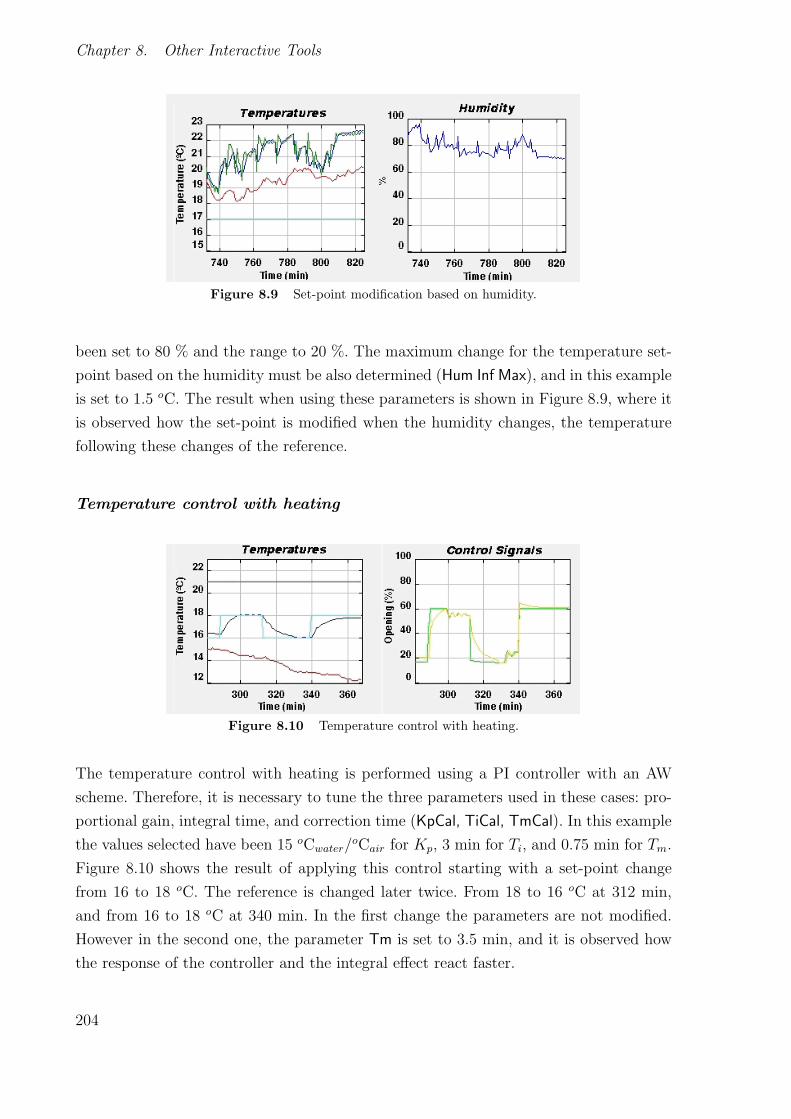
Chapter 8. Other Interactive Tools
Figure 8.9 Set-point modification based on humidity.
been set to 80 % and the range to 20 %. The maximum change for the temperature set-
point based on the humidity must be also determined (Hum Inf Max), and in this example
is set to 1.5 oC. The result when using these parameters is shown in Figure 8.9, where it
is observed how the set-point is modified when the humidity changes, the temperature
following these changes of the reference.
Temperature control with heating
Figure 8.10 Temperature control with heating.
The temperature control with heating is performed using a PI controller with an AW
scheme. Therefore, it is necessary to tune the three parameters used in these cases: pro-
portional gain, integral time, and correction time (KpCal, TiCal, TmCal). In this example
the values selected have been 15 oCwater/oCair for Kp, 3 min for Ti, and 0.75 min for Tm.
Figure 8.10 shows the result of applying this control starting with a set-point change
from 16 to 18 oC. The reference is changed later twice. From 18 to 16 oC at 312 min,
and from 16 to 18 oC at 340 min. In the first change the parameters are not modified.
However in the second one, the parameter Tm is set to 3.5 min, and it is observed how
the response of the controller and the integral effect react faster.
204

8.1.4 Illustrative Examples
Figure 8.11 Radiation control with shade screen.
Radiation control with shade screen
In order to control the radiation with shade screen, an on/off controller with dead zone
has been implemented. In this case there are only two parameters, the value of the dead
zone (Rad Dead-Zone) and the radiation set-point. Initially, the set-point has been set
to 60 W/m2 and the dead zone to 7.5 W/m2. The result of this example is shown in
Figure 8.11 where it can be seen how using these values, the shade screen is closed during
a lot of time. In the minute 895 the dead zone is reduced to 5 W/m2, and the shade
screen remains closed up to minute 945 when the radiation leaves the dead zone causing
several times the opening and closing of the shade screen.
Figure 8.12 Study of extreme conditions.
Extreme situations
The different actions which would be necessary to perform in presence of extreme situa-
tions can be studied in the tool. One of them it is the possibility of limiting the ventilation
opening (WSmaxOpen) when the wind speed exceeds a determined value (WSmax). An
example it is shown in Figure 8.12 where the ventilation opening has been limited to 10
% when the wind speed exceeds 4 m/s. This effect is observed from minute 906.
205

Chapter 8. Other Interactive Tools
8.2 Mobile Robotics Interactive Tool
Mobile robotics involves the problem of moving a mobile robot in any environment
following a free collision path. It involves many tasks related to algorithms in path plan-
ning, knowledge representation, sensing, and reasoning. For this reason, mobile robotics
combines many disciplines, including electrical engineering, automatic control, computer
science, mechanical engineering, artificial intelligent, and others [93]. Mobile robotics
can be understood as a navigation problem, described as the action of directing a mobile
robot to traverse a specific environment. The main aim in any navigation scheme is to
reach a destination without moving away from the goal or crashing with objects [122],
[120]. Navigation is divided into three tasks: mapping, planning, and tracking. If the map
of the environment is considered as an input to the system (the mapping problem has
been solved), the navigation process in mobile robotics involves two kind of problems:
• Path planning. It is a geometric problem related with the robot dimensions and
the obstacles located in the navigation space. Its solution provides a sequence of
positions that joins the initial and goal points defining the free trajectory (without
obstacles) to follow by the robot.
• Path tracking. It is a control problem related with the constraints of the robot
movements, actuators and the time elapsed in the navigation. Its solution provides,
all the time, the set point to each actuator aimed at reaching or following in a
determined time the trajectory obtained when solving the geometric problem.
The solution of the path planning task depends on the knowledge the robot has of
the navigation space. Global algorithms will be used if the dimensions and locations
of all the obstacles are well-known (deliberative navigation). If this information is un-
known, the use of local algorithms (reactive navigation) is required. With both global
and local algorithms it is necessary to know or estimate the robot position at each time.
In real applications different techniques and/or sensors are used to obtain the actual
robot position (odometry, inertial methods, DGPS, etc.). The integration of the robot
kinematics or dynamics provides an approximation to the real position that can be used
for simulation purposes.
Therefore, mobile robotics involves many disciplines and the navigation problem re-
quires several steps that must be well studied and understood by engineering students.
Based on the author’s experience, the teaching and learning of the involved concepts
could be handled using the new interactive methodologies presented in previous chapters.
206
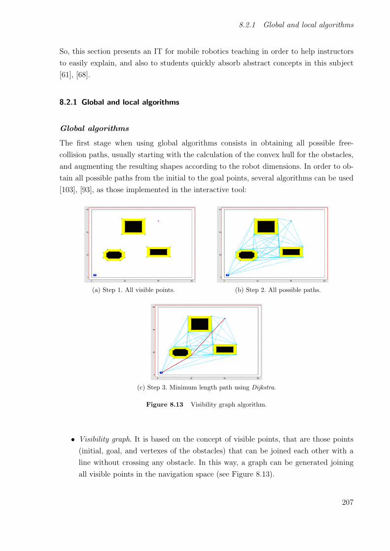
8.2.1 Global and local algorithms
So, this section presents an IT for mobile robotics teaching in order to help instructors
to easily explain, and also to students quickly absorb abstract concepts in this subject
[61], [68].
8.2.1 Global and local algorithms
Global algorithms
The first stage when using global algorithms consists in obtaining all possible free-
collision paths, usually starting with the calculation of the convex hull for the obstacles,
and augmenting the resulting shapes according to the robot dimensions. In order to ob-
tain all possible paths from the initial to the goal points, several algorithms can be used
[103], [93], as those implemented in the interactive tool:
(a) Step 1. All visible points. (b) Step 2. All possible paths.
(c) Step 3. Minimum length path using Dijkstra.
Figure 8.13 Visibility graph algorithm.
• Visibility graph. It is based on the concept of visible points, that are those points
(initial, goal, and vertexes of the obstacles) that can be joined each other with a
line without crossing any obstacle. In this way, a graph can be generated joining
all visible points in the navigation space (see Figure 8.13).
207
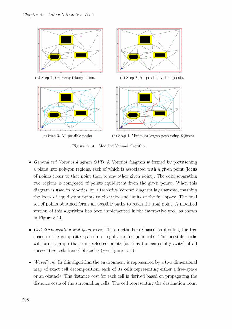
Chapter 8. Other Interactive Tools
(a) Step 1. Delanuay triangulation. (b) Step 2. All possible visible points.
(c) Step 3. All possible paths. (d) Step 4. Minimum length path using Dijkstra.
Figure 8.14 Modified Voronoi algorithm.
• Generalized Voronoi diagram GVD. A Voronoi diagram is formed by partitioning
a plane into polygon regions, each of which is associated with a given point (locus
of points closer to that point than to any other given point). The edge separating
two regions is composed of points equidistant from the given points. When this
diagram is used in robotics, an alternative Voronoi diagram is generated, meaning
the locus of equidistant points to obstacles and limits of the free space. The final
set of points obtained forms all possible paths to reach the goal point. A modified
version of this algorithm has been implemented in the interactive tool, as shown
in Figure 8.14.
• Cell decomposition and quad-trees. These methods are based on dividing the free
space or the composite space into regular or irregular cells. The possible paths
will form a graph that joins selected points (such as the center of gravity) of all
consecutive cells free of obstacles (see Figure 8.15).
• WaveFront. In this algorithm the environment is represented by a two dimensional
map of exact cell decomposition, each of its cells representing either a free-space
or an obstacle. The distance cost for each cell is derived based on propagating the
distance costs of the surrounding cells. The cell representing the destination point
208

8.2.1 Global and local algorithms
(a) Step 1. Cell decomposition. (b) Step 2. Central points.
(c) Step 3. All possible paths. (d) Step 4. Minimum length path using Dijkstra.
Figure 8.15 Cell decomposition algorithm.
is given a distance cost equal to zero. All other cells are initially set to a very high
value. The process is constructed as a two step traversal of the 2D map array: a
forward raster order step (left to right, top to bottom), and a reverse raster order
step (right to left, bottom to top). In each step, each free-space cell (obstacles
are skipped) is assigned a value of one greater than the least value of the four
neighbors previously visited on that step, this assignment occurs only if the new
value is less than the previous value at that cell. Both steps are repeated until
no further changes to cell assignment occur. The final distance cost at each cell
represents the minimum number of cell steps to the destination cell. The optimal
path can be found from any starting point by looking at its 8-neighbor cells and
moving to the one with the lowest distance cost. This process is repeated until the
destination cell is reached (see Figure 8.16) [110].
Once the possible paths have been calculated, the next step consists on calculating the
optimum path according to a certain criteria: minimum distance, minimum curvature,
etc. The criteria selected in the tool has been the minimum distance and the Dijkstra
algorithm has been used to compute it. This algorithm has been modified to achieve
fast computing times admissible for interactive tools. The following step is to calculate
209
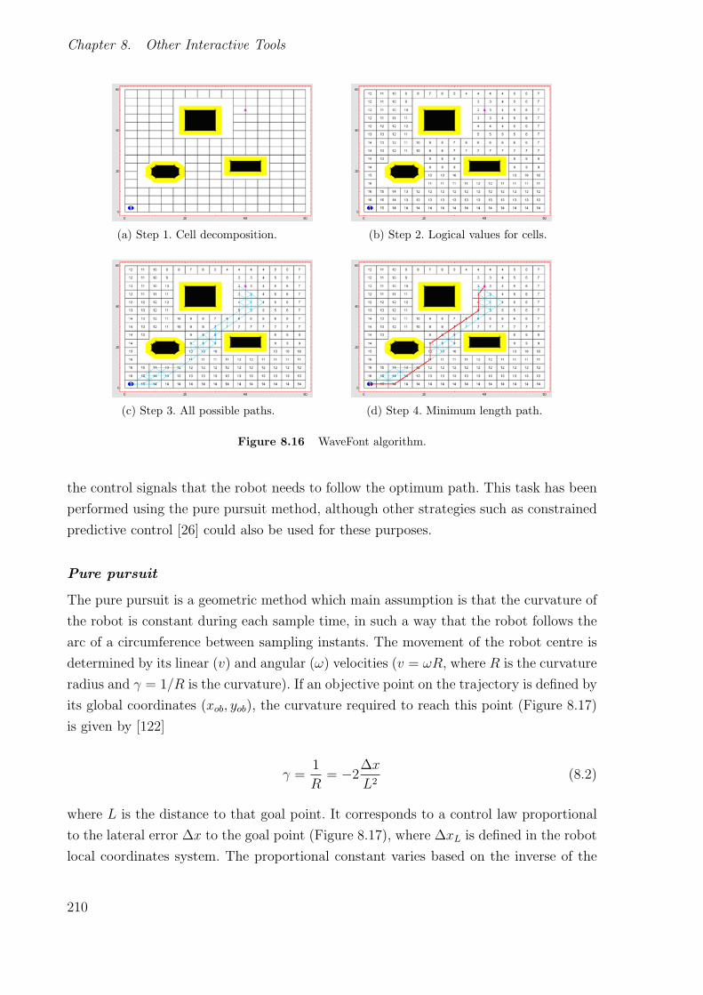
Chapter 8. Other Interactive Tools
(a) Step 1. Cell decomposition. (b) Step 2. Logical values for cells.
(c) Step 3. All possible paths. (d) Step 4. Minimum length path.
Figure 8.16 WaveFont algorithm.
the control signals that the robot needs to follow the optimum path. This task has been
performed using the pure pursuit method, although other strategies such as constrained
predictive control [26] could also be used for these purposes.
Pure pursuit
The pure pursuit is a geometric method which main assumption is that the curvature of
the robot is constant during each sample time, in such a way that the robot follows the
arc of a circumference between sampling instants. The movement of the robot centre is
determined by its linear (v) and angular (ω) velocities (v = ωR, where R is the curvature
radius and γ = 1/R is the curvature). If an objective point on the trajectory is defined by
its global coordinates (xob, yob), the curvature required to reach this point (Figure 8.17)
is given by [122]
γ =1
R= −2
∆x
L2(8.2)
where L is the distance to that goal point. It corresponds to a control law proportional
to the lateral error ∆x to the goal point (Figure 8.17), where ∆xL is defined in the robot
local coordinates system. The proportional constant varies based on the inverse of the
210

8.2.1 Global and local algorithms
square of L. Once the desired curvature has been obtained, the next step will be to obtain
the control signals to the actuators depending on the robot configuration treated in the
next section. As the trajectory coordinates and goal point in the trajectory (xob,yob) are
defined using a global reference system, it is necessary to take into account the robot
orientation φ to obtain ∆x
∆x = (xob − x) cosφ+ (yob − y) sinφ, L =√
(xob − x)2 + (yob − y) (8.3)
Figure 8.17 Pure pursuit method.
A practical method to apply the control law [122], is to determine at each sampling
time the global coordinates of the robot (x, y), to obtain the nearest point to the robot
belonging to the trajectory (xobm, yobm) and to select as next objective point in the
trajectory (xob, yob) placed at a distance d on the path from (xobm, yobm). Then L is
calculated and the control law (8.2) can be applied.
Local algorithms
Local algorithms have as objective to guide the robot through an unknown environment
using only the information provided by its sensors. The main advantage against global
algorithms are that the required computational power is much smaller and are easier to
implement. The main drawback is that, in general, the solution (reaching the goal point)
cannot be guaranteed, even if this exists (only some types of methods like BUG ones can
provide some figures regarding convergence). The following local algorithms have been
considered in the tool [93], [103]:
211

Chapter 8. Other Interactive Tools
(a) Potential algorithm. (b) BUG algorithm.
(c) VISBUG algorithm.
Figure 8.18 Local algorithms.
• Potential function. It is based on the idea that the robot moves within a ”field of
forces”. The goal point acts as an attraction pole while the obstacles are repulsion
surfaces for the robot. A composition of attraction and rejection forces is performed
to obtain the direction of the displacement all the time (see Figure 8.18(a)).
• BUG. The robot is provided with contact sensors when using this method, and
tries to reach the goal point straight forward. The robot surrounds the detected
obstacles until reaching again the straight line joining the initial and goal points,
following it until finding a new obstacle and so on (see Figure 8.18(b)).
• VISBUG. It is a modification to the BUG algorithm but using finite range distance
sensors, in such a way that it is not necessary to contact with the obstacles. So,
direction changes are performed in advance and non-convex zones of the obstacles
are avoided (see Figure 8.18(c)).
It is also possible to combine global and local algorithms, although this fact has not
been implemented in the tool: the first ones can be used to obtain a minimum length
path within a known environment and once the path tracking has started, the local
algorithms can be used to avoid collisions with unknown obstacles.
212

8.2.2 Robot kinematics
(a) Differential. (b) Tricycle. (c) Synchronous.
Figure 8.19 Robot configurations.
8.2.2 Robot kinematics
The implementation of the path planning and tracking tasks requires the estimation of
the robot position in relation to the same absolute reference system where the coor-
dinates of the trajectories are defined. The kinematic model of the robot are used to
estimate the robot position (x, y) and orientation (φ) all the time (at each sampling time
when implementing digital control, with discrete versions of the kinematics, as done in
this work). As has been pointed out in the previous section, in all the cases the robot
displacement is determined by its linear (v) and angular (ω) velocities in such a way
that, if the linear velocity is fixed, knowing the desired curvature from the pure pursuit
(or other) method, ω can be determined and thus the robot displacement. The robot
kinematics are described as discretized versions of the following descriptions[122]:
• Differential mechanism (Figure 8.19(a)). The robot has two motored wheels, so that
the control variables are the angular speed of each one (ωi, ωd). The kinematics
are described by
x′ =−r sinφ
wωi − r sinφ
wωd, y′ =
r cosφ
wωi +
r cosφ
wωd, φ′ =
−rbωi +
r
bωd (8.4)
where x′, y′, and φ′ represents the time derivative of the robot position (x, y) and
orientation φ, r is the wheel radius, and b is the separation of the wheels. The
relation with v and ω is
ωi =v − (b/2)ω
r, ωd =
v + (b/2)ω
r(8.5)
• Tricycle/Ackermann (Figure 8.19(b)). This kind of robots has three/four wheels:
one/two in the front (motorized and directional wheels) and two wheels in the
back. The kinematics are given by the discrete version of
213

Chapter 8. Other Interactive Tools
x′ = −v sinφ, y′ = v cosφ, φ′ = vγ (8.6)
The control signals in this configuration are the direction angle α and the angular
velocity of the directional wheel ωt, given by
ωt =vtr
=
√v2 + ω2l2
r, α = atan(γl) (8.7)
where l is the robot length and r is the radius of the directional wheel.
• Synchronous (Figure 8.19(c)). It contains transmissions to allow positioning all the
wheels with an angular speed ω simultaneously, and moving the robot with a linear
speed v. The kinematics are given by the discretization of
x′ = −v sinφ, y′ = v cosφ, φ′ = ω (8.8)
being the control signal the angular speed ω.
8.2.3 Description of the tool
This section describes the main features of the tool, programmed with SysQuake [125].
The main window of the tool is divided into several sections represented in Figure 8.20
(basic screen of the tool) which are described in what follows:
• Environment : main graphic on the right side of the screen. It represents the envi-
ronment with a set of obstacles where the robot will evolve. It is possible to change
the morphology of the obstacles dragging with the mouse over their corners. The
original objects are shown in black, their convex envelopes are drawn using dotted
lines, and the final object (the convex obstacle enlarged using the robot width) are
presented in yellow. Both the origin point (the robot) and the target point that
the robot will try to reach can be modified over this graphic. The results of the
selected planning algorithm are shown on the environment. The shortest path is
drawn in red (for the global algorithms), and the path followed by the robot in
green colour.
• Operation selection: two operation modes are available in the tool and can be mod-
ified using this option. The Configuration mode allows defining the environment,
algorithms, and robots options before running a simulation. The Algorithm mode
is used in order to calculate the minimum length path and run the simulation.
214

8.2.3 Description of the tool
Figure 8.20 Main window of the tool showing an example.
• Algorithm selection and parameters: these two options allow choosing the desired
planning algorithm and modifying its associated parameters. The parameters of
the pure pursuit algorithm can also be changed.
• Robot parameters and kinematics: the different robot parameters such as size,
speed, orientation, and wheel radio can be modified. On the other hand, it is
possible to choose the robot morphology between differential mechanism, tricycle
and synchronous.
• Obstacle insertion: it allows inserting a new obstacle into the environment, this
option being available on the left-bottom corner of the tool. First, the morphology of
the obstacle is selected between several options: triangle, rectangle, or free polygon.
After this selection, the mouse pointer can be placed on the environment location
in which the obstacle will be inserted, and then a single click on the left mouse
button will perform the action. In the case of the free polygon option, the number
of sides must be selected using the slider Sides.
• Control signals : two graphics on the bottom right of the interface (Figure 8.20)
215

Chapter 8. Other Interactive Tools
show the evolution of the control signals of the selected kinematics (the angular
velocity of the left and right wheels ωi and ωd in Figure 8.20, because the differential
kinematic is chosen). Amplitude and/or rate input constraints can be included by
dragging the red vertical lines shown in the graphs.
• Menu Settings : it is possible to start, pause, and stop the simulation and to show
the results step by step. Also, all the options available in the graphical interface
can also be modified from this menu.
8.2.4 Illustrative Examples
Several examples are shown in this section to demonstrate the main capabilities of the
tool.
(a) Visibility graph. (b) Voronoi diagram.
(c) Cell decomposition. (d) WaveFront.
Figure 8.21 Tracking examples for global algorithms.
Global algorithms
The environment shown in Figures 8.13-8.16 incorporates all the steps related to the
application of global path planning algorithms (calculation of the convex hull, obstacles
enlarging, determination of initial and goal points, and all possible paths), as well as the
minimum path calculation. The minimum length trajectory is obtained using the Dijkstra
216

8.2.4 Illustrative Examples
algorithm and it is shown in red colour. The tracking of this trajectory is performed using
the pure pursuit method after selecting the desired robot kinematics and Run option from
the Setting menu. Figure 8.21 shows the results obtained using differential kinematics for
all global algorithms for the same environment that in Figures 8.13-8.16. The tool allows
studying the differences between the three available global algorithms. For the previous
results, the visibility graph algorithm provides the shortest and smoothest path, while
the modified Voronoi algorithm the longest and most angular one. However, from a safety
point of view, the Voronoi and wavefront algorithms provide the best results.
(a) Visibility graph. (b) WaveFront.
(c) BUG. (d) Potential.
Figure 8.22 Effect of environment modification in different algorithms.
Obstacles insertion
The tool allows modifying, including, and deleting objects in the environment. Once
any of these actions is performed the used algorithm must take into account the new
conditions to find the final point. In the case of global algorithms, it is necessary to
calculate the new possible ways for determining if some of them are more optimal than the
previous path obtained. When using local algorithms the changes are not so important
since the robot has no knowledge of any modification in the environment. Figure 8.22
shows the effect of environment modifications for the examples of Figures 8.13, 8.16, and
8.18, for global and local algorithms.
217
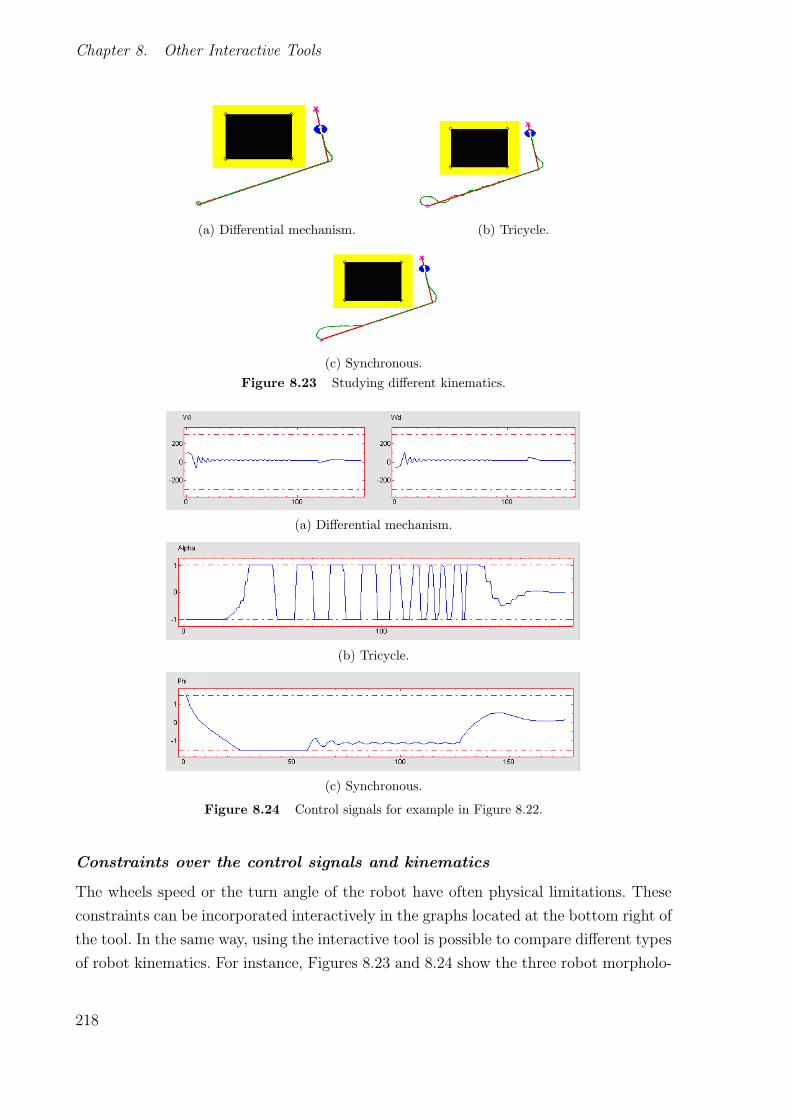
Chapter 8. Other Interactive Tools
(a) Differential mechanism. (b) Tricycle.
(c) Synchronous.Figure 8.23 Studying different kinematics.
(a) Differential mechanism.
(b) Tricycle.
(c) Synchronous.
Figure 8.24 Control signals for example in Figure 8.22.
Constraints over the control signals and kinematics
The wheels speed or the turn angle of the robot have often physical limitations. These
constraints can be incorporated interactively in the graphs located at the bottom right of
the tool. In the same way, using the interactive tool is possible to compare different types
of robot kinematics. For instance, Figures 8.23 and 8.24 show the three robot morpholo-
218
8.3 Conclusions
gies and the control actions associated to each kinematics. In the cases of tricycle and
synchronous kinematics some physical limitations have been taken into account. From
the results, it can be summarized that the differential mechanism kinematics is the only
one that provides turn angle equal to zero. It can also be seen the bad behavior of the
tricycle one, due to its large turn angle (only one free wheel) and the constraints imposed
during the simulation.
8.3 Conclusions
This chapter describes how Interactivity can be applied to other frameworks related with
Automatic Control. There exits several areas where basic control concepts are explained
to the students in short time periods and usually as complementing education. Hence,
Interactivity can play an important role in these cases where theoretical concepts can be
abstracted in Interactive synoptics making the learning more familiar to the students.
In this way, a couple of IT have been developed as support to the education in the
Greenhouse Climatic Control and Mobile Robotics fields.
These tools have been used in university courses during the last two years. Students
have paid a great attention to these IT, their learning being considerably improved. The
feedback obtained from the students has also been used to improve both the design and
performance of the tools.
219

9
Conclusions and future works
The objectives of this thesis were to provide, on one hand, new approaches and outreaches
to the Automatic Control education community by means of a set of IT developed to
help in the dissemination of basic (PID control) and advanced (GPC) control concepts.
A deep reflection about the role of interactivity in Automatic Control education has been
accomplished, as a previous step in the development of methods and tools useful both
for teachers and students. The same applies to other interesting issues such as the use
of examples, the understanding of theory through visualization, etc. On the other hand,
looking for computationally efficient MPC approaches to handle uncertainties, a new ro-
bust suboptimal MPC approach has been developed mixing GPC and QFT, where differ-
ent solutions have been proposed to face robust constrained predictive control problems.
Some of them are based on transfer function representations being both computationally
efficient and useful for industrial applications. Due to the lack of rigorous results about
constrained robust stability using the transfer function representations, the GPC-QFT
approach has also been solved by means of LMI solutions for robust predictive control,
considering input constrains in the inner loop and tracking problems. The LMI-based
solutions have provided efficient results ensuring constrained robust stability. Thus, the
main contributions of the thesis have been done within the framework of these fields of
education and robust MPC.
In the field of Automatic Control education, the contributions can be summarized in
the following IT:
• PID Basics. It is an interactive module designed to make students familiar with
PID control. The module gives time and frequency domain views of the responses
of a closed-loop system consisting of a PID controller and a process model. Many
process models can be selected, controller parameters can be changed interactively,
and the resulting responses can be displayed instantaneously.
• PID LoopShaping. Loop shaping is a design method where it is attempted to choose
a controller such that the loop transfer function fits the desired shape. In this mod-
221
Chapter 9. Conclusions and future works
ule the loop transfer function is illustrated by its Nyquist plot. Free and constrained
designs can be performed where students may study sensitivity properties for the
compensated system.
• PID Windup. Many aspects of PID control can be understood using linear models.
There are, however, some important nonlinear effects that are very common even
in simple loops with PID control. Integral windup can occur in loops where the
process has saturations and the controller has integral action. The purpose of this
module is to easily explain the phenomenon of integral windup and a method for
avoiding it.
• SISO-GPCIT. Its objective is to help the students to learn and understand the
basic concepts involved in GPC. With this tool the student can put into practice
the adquired knowledge on this control technique using simple examples of uncon-
strained cases, effect of plant/model mismatch and robustness issues, disturbance
rejection, effect of constraints in the design and performance of the controller,
stability issues, etc.
• MIMO-GPCIT. It is an IT to facilite the understanding of MIMO systems con-
trolled with GPC. The tool allows working with the main aspects of constrained
predictive control, studying typical problems associated with MIMO and SISO
systems. Students can use the tool to study different problems by means of a
cause-effect relation. Some of the features about multivariable systems which can
be analyzed using the tool are: control parameters effect on the relative time scales
of the different system outputs, feasibility problems that may appear due to con-
straint violation of some variables, how feasibility problems can be avoided studying
the effect of imposing constraints on other system variables, or pole-zero represen-
tation of a transfer matrix for a multivariable system, observing system behaviors
which are usually very difficult to detect (for instance, non-minimum phase).
All these tools have demonstrated to be very useful for Automatic Control education.
The GPC tools have been used in process control courses during the last two years,
receiving a great attention and acceptance by the students, as indicated in surveys and
tests provided to them when finishing the courses. In fact, the combined use of IT with
classical programming lab sessions (using Matlab) has been very successful, as the IT
have become a way to test the correctness of the algorithms and calculus performed
by the students. The repercussion of the IT in the classrooms has been such that we
have been almost forced to developed new tools for the different courses covered by
the Automatic Control unit of our university. In this way, different IT have been also
222

designed and developed to cover aspects such as mobile robotics, climate control, etc.
These IT have been complemented with remote labs and classical lectures. Two of these
IT have been included in this document as a way to demonstrate that the methodology
and concepts involved in the use of interactivity in Automatic Control education are
easily applicable to different educational fields. The references include other works made
by the author in cooperation with other colleagues related to the influence of NICT in
Automatic Control education.
The second contribution within the field of robust MPC has been materialized in
both control structures and methods, and IT:
• A new control approach mixing GPC and QFT has been developed for controlling
a family of linear uncertain plants. A cascaded structure is proposed, combining an
inner loop containing a QFT controller with an outer loop where a GPC controller
provides adequate references for the inner loop. In the approximation proposed in
this thesis, a nominal GPC is used to control a plant with uncertainties, where a
QFT controller is placed in the inner loop to reduce the uncertainties in the family
of the plants, augmenting the robust stability of GPC, which is analyzed using the
RRL method and the SGT.
• Some modifications in the basic structure of GPC have been performed in order
to manage the inner loop input constraints. The proposed structures in the GPC-
QFT approach are based on using GPC as set-point generator combined with
different techniques: AW [5], robust online identification [17], hard constraints, and
constraints softening [107].
• RGPCQFT-IT. It is an IT which implements the GPC-QFT approach presented
in this thesis, being possible to implement a fast robust predictive control solution.
The proposed approach has been implemented in an IT in order to show its low
computational load and study some heuristic parameters involved in it.
• The obtained results in the GPC-QFT approach using transfer function repre-
sentations have the problem that it is quite difficult to formalize the results in
order to ensure constrained robust stability. Hence, a state space representation
for the GPC-QFT approach has been obtained in order to use the results of ro-
bust predictive control by means of LMI. In this way, a robust stable solution for
the GPC-QFT approach solving tracking problems and with input constraints has
been developed.
All the previous works have been materialized in publications in journal and conferences.
223

Chapter 9. Conclusions and future works
9.1 Future works
Nowadays, there is a renewed interest in Automatic Control education. The research
works in this direction should continue in order to help students to learn and improve
the teaching methods. Interactivity has demonstrated to be a very important factor as
support to control education. The objective of IT is to encourage control engineering
students to think and interact with the examples in other way they do in the case of
textbooks or lecture presentations. Because the examples can be used in an unsupervised
environment, simplicity and clarity are key features. The scenario for control education
is changing and teachers must adapt to these changes. Information technology opens a
whole new world of real opportunities. Computers show a great potential to enhance
student achievement, but only if they are used appropriately as part of a coherent edu-
cational approach. Computers do not change in the way books or labs do, they allow us
to go deeper and faster. In order to complete a full course on Automatic Control, a set
of new interactive tools are proposed as future works:
• Interactive Modelling Module, in order to introduce basic concepts about modelling
in relation with Automatic Control.
• PID Design Interactive Module, where different design methods for PID control
can be studied and compared.
• Predictor Interactive Module, in order to study delayed control systems. The idea
would be to work with PID, PPI, Smith Predictor, and predictive algorithms.
• Control Coupled Loops Interactive Module, where the main concepts about multi-
variable control could be introduced.
• Feedforward Interactive Module, in order to introduce how feedforward control can
compensate for measurable disturbances.
• Identification and Adaptive Control Interactive Module, where the main aspects
about model identification and adaptive control will be presented.
In this way, the modules will make the key pictures in the book Advanced PID Control
[5] interactive, obtaining a very rich combination between theoretical concepts (book)
and practical exercises (interactive modules).
On the other hand, the proposed GPC-QFT algorithm has presented a high compu-
tational efficiency and an easy implementation. Different ways have been proposed to
224

9.1 Future works
solve the mixed GPC-QFT approach showing the results via simulations, where some of
them ensure constrained robust stability and others are based on heuristic solutions. So,
such conclusions open possible future works related with this topic:
• Perform real tests in order to verify the low computational load that has been
studied by simulation. Furthermore, comparisons with other techniques could be
performed in order to observe the differences in computational efficiency and per-
formance.
• Application of the proposed approach to bilinear plants. These plants can be ap-
proximated as linear ones by means of feedback linearization approaches. Then,
once the plant is linearized, the proposed GPC-QFT approach could be used to
control the linearized system. A greenhouse [137] and a distributed collector field
[24] are a couple of real processes available for the author in his research group. Such
processes can be approximated by bilinear models where the previous commented
strategy could be implemented.
225

10
Bibliography
[1] J. Adeel. Redes y Educacion. Nuevas Tecnologıas, Comunicacion Audiovisual y
Educacion. Cedecs, 2002.
[2] T. Alamo, J.L. Guzman, M. Berenguel, and S. Dormido. Stable constrained robust
GPC-QFT approach using LMIs. Internal Report. University of Seville/University
of Almerıa/UNED, 2006.
[3] P. Ansay, M. Gevers, and V. Wertz. Enhacing the robustness of GPC via simple
choice of the Youla parameter. European Journal of Control, 4(64-70), 1998.
[4] P. Ansay and V. Wertz. Model uncertainties in GPC: A systematic two-step design.
Proceedings of the European Control Conference ECC97, 1997. Brussels (Belgium).
[5] K.J. Astrom and T. Hagglund. Advanced PID Control. ISA - The Instrumentation,
Systems, and Automation Society. Research Triangle Park, NC 27709, 2005.
[6] K.J. Astrom. Automatic Control - The Hidden Technology in book Advances in
Control, Highlights of ECC99, pages 1–28. Springer, London, 1999.
[7] K.J. Astrom. Introduction to Control. Department of Automatic Control. Lund
Institute of Technology, 2004.
[8] P. Banerjee and S.L. Shah. Tuning guidelines for robust generalized predictive
control. Proceedings of the IEEE Conference on Decision and Control CDC92,
1992. Tucson, Arizona (USA).
[9] P. Banerjee and S.L. Shah. The role of signal processing methods in the robust
design of predictive control. Automatica, 31(5):681–695, 1995.
[10] P. Barker. Designing Interactive Learning, in T. de Jong & L. Sarti (Eds), Design
and Production of Multimedia and Simulation-based Learning Material. Kluwer
Academic Publishers, 1994.
227

Chapter 10. Bibliography
[11] B.R. Barmish and R. Tempo. The Robust Root Locus. Proceedings of the IEEE
Conference on Decision and Control CDC88, 1988. Austin, Texas (USA).
[12] A. Bemporad, F. Borreli, and M. Morari. Model predictive control based on linear
programming. The explicit solution. IEEE Transactions on Automatic Control,
47(12):1974–1985, 2002.
[13] A. Bemporad, M. Morari, V. Dua, and E.N. Pistikopoulos. The explicit linear
quadratic regulator for constrained systems. Automatica, 38(1):3–20, 2002.
[14] A. Bemporad. Reference governor for constrained nonlinear systems. IEEE Trans-
actions on Automatic Control, 43(3):415–419, 1998.
[15] S. Bennett. A Brief history of Automatic Control. IEEE Control System Magazine,
16(3):17–25, 1996.
[16] M. Berenguel, F. Rodrıguez, J.L. Guzman, J. Perez-Parra, and D. Lacasa. Green-
house diurnal temperature control with natural ventilation based on empirical mod-
els. Proceedings of the International Symposium on Greenhouse Cooling: methods,
technologies and plant response, 2006. Almerıa (Spain).
[17] M. Berenguel. Contributions to the Control of Distributed Solar Collectors, (in
Spanish, Contribuciones al Control de Colectores Solares Distribuidos). Phd thesis,
ETSII, University of Seville, Spain (Universidad de Sevilla, Espana), 1995.
[18] H.S. Black. Stabilized Feedback Amplifiers. Bell System Technology Journal, pages
114–120, 1934.
[19] P. Booth. An Introduction to Human-Computer Interaction. Lawrence Erlbaum,
1989.
[20] C. Borghesani, Y. Chait, and O. Yaniv. The QFT Frequency Domain Control
Design Toolbox. User’s Guide. Terasoft, Inc., 2003.
[21] T. Borsook and N. Higginbotham-Wheat. Interactivity: what is it and what can it
do for computer-based instruction. Educational Technology, 31(10):11–17, 1991.
[22] S. Boyd, L. El Ghaoui, E. Feron, and V. Balakrishnan. Linear Matrix Inequalities
in System and Control Theory, volume 15. Society for Industrial and Applied
Mathematics, SIAM, 1994.
[23] D. Bricklin and B. Frankston. VisiCalc ’79. Creative Computing, 1984.
228
[24] E.F. Camacho, M. Berenguel, and F.R. Rubio. Advanced Control of Solar Plants.
Springer, 1997.
[25] E.F. Camacho and M. Berenguel. Robust adaptive model predictive control of a
solar plant with bounded uncertainties. International Journal of Adaptive Control
and Signal Processing, 11(4):311–325, 1997.
[26] E.F. Camacho and C. Bordons. Model Predictive Control. Springer, 2004.
[27] P.J. Campo and M. Morari. Robust model predictive control. Proceedings of the
American Control Conference ACC87, 1987. Minneapolis, Minnesota (USA).
[28] D.W. Clarke, C. Mohtadi, and P.S. Tuffs. Generalized predictive control - parts I
and II. Automatica, 23(2):137–160, 1987.
[29] D.W. Clarke and C. Mohtadi. Properties of generalized predictive control. Auto-
matica, 25(6):859–875, 1989.
[30] D.W. Clarke and R. Scattolini. Constrained receding-horizon predictive control.
IEE Proceedings Part D, Control Theory and Applications, 138(4):347–354, 1991.
[31] D.W. Clarke. Designing robustness into predictive control. Proceedings of the IEE
Colloquium on Industrial Applications of Model Based Predictive Control, 1991.
London (UK).
[32] S.G. Crutchfield and W. J. Rugh. Interactive learning for signal, systems, and
control. IEEE Control Systems Magazine, 18:88–91, 1998.
[33] J.M. Dıaz, S. Dormido, and J. Aranda. Interactive computer-aided control design
using quantitative feedback theory: the problem of vertical movement stabilization
on a high-speed ferry. International Journal of Control, 78(11):813–825, 2005.
[34] J.M. Dıaz, S. Dormido, and J. Aranda. Quantitaive Feedback Theory Interactive
tool for SISO systems. Technical report, UNED, Spain.
[35] K. Diehl, B. Krogh, and M. Nagurka. An interactive control systems simulator.
IEEE Control Systems Magazine, 6(2):20–26, 1986.
[36] Docenweb. Red Tematica de Docencia en Control mediante Web. Accion especial
del MCYT (DPI2002-11505-E), 2003-2004.
[37] S. Dormido and F. Esquembre. The quadruple-tank process: an interactive tool for
control education. Proceedings of the European Control Conference ECC03, 2003.
Cambridge (UK).
229

Chapter 10. Bibliography
[38] S. Dormido, F. Gordillo, S. Dormido Canto, and J. Aracil. An interactive tool for
introductory nonlinear control systems education. Proceedings of the 17th IFAC
World Congress, 2002. Barcelona (Spain).
[39] S. Dormido. Control learning: present and future (Plenary Lecture). Proceedings
of the 17th IFAC World Congress, 2002. Barcelona (Spain).
[40] S. Dormido. The role of interactivity in control learning (Plenary Lecture).
Proceedings of the IFAC Symposium on Advances in Control Education ACE03,
2003. Oulu (Finland).
[41] S. Dormido. Control learning: present and future. Annual Reviews in Control,
28(1):115–136, 2004.
[42] A. Emami-Naeini and G. Franklin. Interactive computer-aided design of control
systems. IEEE Control Systems Magazine, 1(4):31–36, 1981.
[43] F. Esquembre and J. Sanchez. Easy Java Simulations 3.3. How to use Ejs with
Matlab and Simulink. http://fem.um.es/Ejs/, 2004.
[44] H. Fang, Z. Lin, and T. Hu. Analysis of linear systems in the presence of actuator
saturation and L2-disturbances. Automatica, 40:1229–1238, 2004.
[45] D. Frederick, R. Kraft, and T. Sadeghi. Computer-aided control system analysis
and design using interactive computer graphics. IEEE Control Systems Magazine,
2(4):31–36, 1982.
[46] M. Garcıa-Sanz and J.C. Guillen. Smith Predictor for uncertain systems in the
QFT framework. Proceedings of the third European Robotics, Intelligent Systems
and Control Conference EURISCON98, 1998. Athens (Greece).
[47] A.A. Garcıa, M. Berenguel, J.L. Guzman, S. Dormido, and M. Domınguez.
Laboratorio remoto para el proceso de los cuatro tanques y su aplicacion en
docencia de control multivariable. Actas del IV Jornadas de Trabajo ”Ensenanza
Vıa Internet/Web de la Ingenierıa de Sistemas y Automatica”, EIWISA05. Dentro
del I Congreso Espanol de Informatica (CEDI), 2005. Granada (Spain).
[48] A.A. Garcıa, M. Berenguel, J.L. Guzman, S. Dormido, and M. Domınguez. Remote
laboratory for teaching multivariable control techniques. Proceedings of the 7th
IFAC Sympsium on Advances in Control Education ACE06, 2006. Madrid (Spain).
230

[49] D. Gillet, H. A. Latchman, and O.D. Crisalle. Hands-On Laboratory Experiments
in Flexible and Distance Learning. Journal of Engineering Education, pages 187–
191, 2001.
[50] D. Gillet, A. V. Nguyen, and Y. Rekik. Collaborative web-based experimentation
in flexible engineering education. IEEE Transactions on Education, 48(4):696–704,
2005.
[51] R.S. Gilliver, B. Randall, and Y.M. Pok. Learning in cyberspace: shaping the
future. Journal of Computer Assisted Learning, 14(14):212–22, 1998.
[52] J.A. Gil, J.L. Guzman, and V. Ruiz. Una simulacion del procesador MIPS R2000.
Actas de la Jornada sobre Tecnologıas aplicadas a la ensenanza de la Electronica,
TAEE, 2000. Barcelona (Spain).
[53] J.L. Guzman, K.J. Astrom, S. Dormido, T. Hagglund, and Y. Piguet. Interactive
learning modules for PID control. Proceedings of the 7th IFAC Symposium on
Advances in Control Education ACE06, 2006. Madrid (Spain).
[54] J.L. Guzman, M. Berenguel, S. Dormido, and T. Hagglund. A robust constrained
predictive GPC-QFT approach. UAL/UNED/LUND Internal Report, 2006.
[55] J.L. Guzman, M. Berenguel, and S. Dormido. MIMO-GPCIT. Herramienta
interactiva de control predictivo generalizado para sistemas multivariables. Actas
de las XXIV Jornadas de Automatica, 2003. Leon (Espana).
[56] J.L. Guzman, M. Berenguel, and S. Dormido. MIMO-GPCIT. Herramienta
interactiva de control predictivo generalizado para sistemas multivariables. RIAI.
Revista Iberoamericana de Automatica e Informatica Industrial, 1(1):57–69, 2004.
[57] J.L. Guzman, M. Berenguel, and S. Dormido. SISO-GPCIT: Generalized predictive
control interactive tool for SISO systems. http://aer.ual.es/siso-gpcit/, 2004.
UAL/UNED Internal Report.
[58] J.L. Guzman, M. Berenguel, and S. Dormido. Interactive teaching of constrained
generalized predictive control. IEEE Control Systems Magazine, 25(2):79–85, 2005.
Available: http://aer.ual.es/siso-gpcit/.
[59] J.L. Guzman, M. Berenguel, F. Rodrıguez, and S. Dormido. Herramienta interac-
tiva para robotica movil. Actas de las XXIV Jornadas de Automatica, 2003. Leon
(Espana).
231

Chapter 10. Bibliography
[60] J.L. Guzman, M. Berenguel, F. Rodrıguez, and S. Dormido. Web-based remote
control laboratory using a greenhouse scale model. Computer applications in
engineering education, 13(2):111–124, 2005.
[61] J.L. Guzman, M. Berenguel, F. Rodrıguez, and S. Dormido. Interactive teaching
of mobile robotics. Submitted to IEEE Robotics and Automation Magazine, 2006.
[62] J.L. Guzman, M. Berenguel, and F. Rodrıguez. Laboratorio remoto para el control
de una maqueta de invernadero. Actas de las XXIII Jornadas de Automatica, 2002.
Tenerife (Espana).
[63] J.L. Guzman, P. Garcıa, T. Hagglund, S. Dormido, P. Albertos, and M. Berenguel.
Interactive tool for analysis of time-delay systems with dead-time compensators.
Proceedings of the 7th IFAC Sympsium on Advances in Control Education ACE06,
2006. Madrid (Spain).
[64] J.L. Guzman, O. Lopez, M. Berenguel, F. Rodrıguez, and S. Dormido. MRIT
- Mobile Robotics Interactive Tool. http://aer.ual.es/mrit/, 2005. UAL/UNED
Internal Report.
[65] J.L. Guzman, R. Medina, F. Rodrıguez, J. Sanchez-Hermosilla, and M. Berenguel.
Control de la presion de un sistema de pulverizacion movil. Actas del II Congreso
Nacional de Agroingenierıa, 2003. Cordoba (Espana).
[66] J.L. Guzman, R. Medina, F. Rodrıguez, J. Sanchez-Hermosilla, and M. Berenguel.
Pressure control of a mobile spraying system. Spanish Journal of Agricultural
Research, 2(2):181–190, 2004.
[67] J.L. Guzman, F. Rodrıguez, M. Berenguel, and S. Dormido. Laboratorio virtual
para la ensenanza del control climatico de Invernaderos. Actas de las XXV Jornadas
de Automatica, 2004. Ciudad Real (Espana).
[68] J.L. Guzman, F. Rodrıguez, M. Berenguel, and S. Dormido. MRIT: Mobile Robot
Interactive Tool. Proceedings of the IFAC Workshop on Internet-Based Control
Education IBCE04, 2004. Grenoble (France).
[69] J.L. Guzman, F. Rodrıguez, M. Berenguel, and S. Dormido. Laboratorio virtual
para la ensenanza del control climatico de invernaderos. RIAI. Revista Iberoamer-
icana de Automatica e Informatica Industrial, 2(1):82–92, 2005.
[70] J.L. Guzman, F. Rodrıguez, M. Berenguel, and S. Dormido. Virtual lab for teaching
greenhouse climatic control. Proceedings of the 16th IFAC World Congress, 2005.
Prague (Czech Republic).
232

[71] J.L. Guzman, J.F. Sarabia, F. Rodrıguez, J.C. Moreno, and M. Berenguel. Entorno
para programacion remota de robots manipuladores en ACL con realimentacion
visual. Actas de las III Jornadas de Trabajo ”Ensenanza Vıa Internet/Web de
Ingenierıa de Sistemas y Automatica”, EIWISA02, 2002. Alicante (Spain).
[72] T. Hagglund and K.J. Astrom. Revisiting the Ziegler-Nichols tuning rules for PI
control. Asian Journal of Control, 4(4):364–380, 2002.
[73] T. Hagglund and K.J. Astrom. Revisiting the Ziegler-Nichols step response method
for PID control. Journal of Process Control, 14(6):635–650, 2004.
[74] T. Hagglund and K.J. Astrom. Revisiting the Ziegler-Nichols tuning rules for
PI control - part II, the frequency response method. Asian Journal of Control,
6(4):469–482, 2004.
[75] T. Hagglund. An industrial dead-time compensating PI controller. Control Engi-
neering Practice, 4(6):749–756, 1997.
[76] B.S. Heck (editor). Enhancing classical control education via interactive GUI
design. IEEE Control System Magazine, 19(3):35–58, 1999.
[77] I.M. Horowitz and M. Sidi. Optimum synthesis of non-minimum phase systems
with plant uncertainty. International Journal of Control, 27(3):361–386, 1978.
[78] I.M. Horowitz. Synthesis of Feedback Systems. Academic Press, 1963.
[79] I.M. Horowitz. Quantitative synthesis of uncertain multiple input-output feedback
systems. International Journal of Control, 30:81–106, 1979.
[80] I.M. Horowitz. A synthesis theory for a class of saturating systems. International
Journal of Control, 38:169–187, 1983.
[81] I.M. Horowitz. Quantitative feeback design theory (QFT). International Journal
of Robust and Non-linear Control, 11(10):887–921, 2001.
[82] C.H. Houpis and S. Rasmussen. Quantitative Feedback Theory: Fundamentals and
Applications. Marcel Dekker, 1999.
[83] C.H. Houpis, R.R. Sating, S. Rasmussen, and S. Sheldon. Quantitative feeback
design theory technique and applications. International Journal of Control, 59:39–
70, 1992.
233
Chapter 10. Bibliography
[84] Q. Hu and G.P. Rangaiah. Anti-windup schemes for uncertain nonlinear systems.
IEE Proceedings Part D, Control Theory and Applications, 147(3):321–329, May
2000.
[85] IEEECSS. IEEE Control System Society. http://www.ieeecss.org/.
[86] IEEECSS. Technical Committee on Control Education. http://www.math.ku.edu/ksacg/
CSS/tcce.html.
[87] IEEE. Innovation in undergraduate education. Part I. Control System Magazine,
24(5), 2004.
[88] IEEE. Innovation in undergraduate education. Part II. Control System Magazine,
25(1), 2005.
[89] IFAC. Special section on advances in control education. Control Engineering
Practice, 14(2), 2006.
[90] IFAC. International Federation of Automatic Control. http://www.ifac-
control.org/.
[91] IFAC. Technical Committee on Control Education. http://www.gu.edu.au/centre/icsl/
edcom/.
[92] A. Isidori. Nonlinear Control Systems. Springer Verlag, 1989.
[93] M. Jenkin and G. Dudek. Computational Principles of Mobile Robotics. Cambridge
University Press, 2000.
[94] M. Johansson, M. Gafvert, and K.J. Astrom. Interactive tools for education in
automatic control. IEEE Control Systems Magazine, 18(3):33–40, 1998.
[95] D. Jonassen. Instructional Designs for Microcomputer Courseware. Lawrence
Erlbaum, 1988.
[96] J.P. Keller. Interactive control system design. Control Engineering Practice,
14:177–184, 2006.
[97] N. A. Kheir, K. J. Astrom, D. Auslander, and K. Cheok. Control system engineering
education. Automatica, 32(2):147–166, 1996.
[98] M.V. Kothare, V. Balakrishnan, and M. Morari. Robust constrained model
predictive control using linear matrix inequalities. Automatica, 32(10):1361–1379,
1996.
234

[99] B. Kouvaritakis, J.A. Rossiter, and A.O.T. Chang. Stable generalized predictive
control: an algorithm with guaranted stability. IEE Proceedings Part D, Control
Theory and Applications, 139(4):349–362, 1992.
[100] B. Kouvaritakis, J.A. Rossiter, and G.J. Ju. Robust stable generalized predictive
control. International Journal of Control, 67(3):411–434, 1997.
[101] M.J. Kurtz and M.A. Henson. Feedback linearizing control of discrete-time non-
linear systems with input constraints. International Journal of Control, 70(4):603–
616, 1998.
[102] A.G. Kuznetsov and D.W. Clarke. Application of Constrained GPC for Improving
the Performance of Controlled Plants, In D. W. Clarke (Ed.), Advances in Model-
based Predictive Control, pages 318–329. Oxford University Press, 1994.
[103] J.C. Latombe. Robot Motion Planning. Kluwer Academic Publishers, 1991.
[104] J.H. Lee and Z. Ju. Worst-case formulations of model predictive control for systems
with bounded parameters. Automatica, 3(5):763–781, 1997.
[105] D. Limon, T. Alamo, and E.F. Camacho. Stable constrained MPC without terminal
constraint. Proceedings of the American Control Conference ACC03, 2003. Denver,
Colorado (USA).
[106] D. Limon, T. Alamo, and E.F. Camacho. Robust stability of min-max MPC
controllers for nonlinear systems with bounded uncertainties. Proceedings of the
Mathematical Theory of Networks and Systems, 2004. Leuven (Belgium).
[107] J. Maciejowski. Constrained Predictive Control. Academic Press, 2002.
[108] P. Marques Graells. Las TICs y sus aportaciones a la sociedad. http://dewey.uab.es/
pmarques/tic.htm, 2000.
[109] P. Marques Graells. Metodologıa didactica y TIC en la ensenanza universitaria.
http://dewey.uab.es/pmarques/caceres.htm, 2004.
[110] C. Martın, A. Urquıa, J. Sanchez, S. Dormido, F. Esquembre, J.L. Guzman,
and M. Berenguel. Interactive simulation of object-oriented hybrid models, by
combined use of Ejs, Matlab/Simulink and Modelica/Dymola. Proceedings of the
18th European Simulation Multiconference, 2004. Magdeburg (Germany).
[111] A.R. Mcintosh, S.L. Shah, and D.G. Fisher. Analysis and tuning of adaptive
generalized predictive control. The Canadian Journal of Chemical Engineering,
68:97–110, 1991.
235

Chapter 10. Bibliography
[112] D. Megıas, J. Serrano, and C. Prada. Uncertainty treatment in GPC: design
of T polynomial. Proceedings of the European Control Conference ECC97, 1997.
Brussels (Belgium).
[113] M. Morari and E. Zafiriou. Robust Process Control. Prentice Hall, 1989.
[114] J.C. Moreno, A. Banos, and M. Berenguel. A synthesis theory for uncertain linear
systems with saturation. Proceedings of the 4th IFAC Symposium on Robust Control
Design, 2003. Milan (Italy).
[115] J.C. Moreno, A. Banos, and M. Berenguel. Robust control for linear systems with
actuator rate and amplitude saturation using QFT. Proceedings of the 4th IFAC
Symposium on Robust Control Design, 2003. Milan (Italy).
[116] J.C. Moreno, M. Berenguel, F. Rodrıguez, J.F. Sarabia, R. Garrote, J.L. Guzman,
and O. Lopez. Proyecto de aplicacion de telerobotica a un mini-robot movil. Actas
de las II Jornadas de Trabajo ”Ensenanza Vıa Internet/Web de Ingenierıa de
Sistemas y Automatica”, EIWISA01, 2001. Madrid (Spain).
[117] J.C. Moreno. Robust Control Techniques for Input Constrained Systems, (in
Spanish, Control Robusto de Sistemas con Restricciones a la Entrada). Phd thesis,
University of Murcia, Spain (Universidad de Murcia, Espana), 2003.
[118] R.M. Murray, K.J. Astrom, S.P. Boyd, R.W. Brockett, and G. Stein. Future
directions in control in a information-rich world. IEEE Control System Magazine,
9(2):20–33, 2003.
[119] D. Munoz de la Pena Sequedo. Model Predictive Control for Uncertain Systems.
Phd thesis, ETSII, University of Seville, Spain (Universidad de Sevilla, Espana),
2005.
[120] U. Nehmzow. Mobile Robotics. Springer, 2003.
[121] J.E. Normey-Rico, C. Bordons, and E.F. Camacho. Improving the robustness of
dead-time compensating PI controllers. Control Engineering Practice, 5(6):801–
810, 1997.
[122] A. Ollero. Robotica. Manipuladores y Robots Moviles. Marcombo, 2001.
[123] H. Panagopoulos. PID Control. Design, Extension, Application. Phd thesis, Lund
University, 2000.
236

[124] M. Pasamontes, F. Rodrıguez, J.L. Guzman, M. Berenguel, and S. Dormido.
Easy mobile device programming for educational purposes. Proceedings of the 44th
IEEE Conference on Decision and Control and European Control Conference CDC-
ECC05, 2005. Seville (Spain).
[125] Y. Piguet. SysQuake 3 User Manual. Calerga S‘arl, Lausanne (Switzerland), 2004.
[126] RAE. Real Academia Espanola de la Lengua. http://www.rae.es/.
[127] A. Ramırez-Arias, F. Rodrıguez, M. Berenguel, and J.L. Guzman. Control
jerarquico multiobjetivo de crecimiento de cultivos en invernadero. In Actas de
las XXVI Jornadas de Automatica 2005, Alicante, Espana, 2005.
[128] A. Ramırez-Arias, F. Rodrıguez, J.L. Guzman, M. Berenguel, M.R. Arahal, and
J.C. Lopez. Improving efficiency of greenhouse heating systems using model
predictive control. Proceedings of the 16th IFAC World Congress, 2005. Prague
(Czech Republic).
[129] D.R. Ramırez, E.F. Camacho, and M.R. Arahal. Implementation of min-max MPC
using hinging hyperplanes: application to a heat exchanger. Control Engineering
Practice, 12:1197–1205, 2004.
[130] D.M. Rhodes and J.W. Azbell. Designing interactive video instruction profession-
ally. Training and Development Journal, 39(12):31–33, 1985.
[131] J. Richalet, A. Rault, J.L. Testud, and J. Papon. Model predictive heuristic control:
applications to industrial processes. Automatica, 14(1):413–428, 1978.
[132] J. Richalet. Industrial applications of model based predictive control. Automatica,
5(29):1251–1274, 1993.
[133] B.D. Robinson and D.W. Clarke. Robustness effects of a prefilter in generalised
predictive control. IEE Proceedings Part D, Control Theory and Applications,
138(1):1–8, 1991.
[134] F. Rodrıguez, M. Berenguel, and M. R. Arahal. A hierarchical control system
for maximizing profit in greenhouse crop production. Proceedings of the European
Control Conference ECC03, 2003. Cambdridge (UK).
[135] F. Rodrıguez, M. Berenguel, J.L. Guzman, and S. Dormido. A virtual course
on automation of agricultural systems. International Journal of Engineering
Education. To appear in 2006.
237

Chapter 10. Bibliography
[136] F. Rodrıguez, J. Sanchez-Hermosilla, A. Sanchez, M. Berenguel, and J.L. Guzman.
Diseno de una plataforma movil para la pulverizacion de productos fitosanitarios
en invernaderos. Actas del III Congreso de AgroIngenierıa, 2005. Leon (Spain).
[137] F. Rodrıguez. Modeling and Hierarchical Control of Greenhouse Crop Growing,
(in Spanish, Modelado y Control Jerarquıco de Crecimiento de Cultivos en
Invernadero). Phd thesis, University of Almerıa, Spain (Universidad de Almerıa,
Espana), 2002.
[138] P. Rodriguez and D. Dumur. Robustification of GPC controlled system by convex
optimisation of the Youla parameter. Proceedings of the International Conference
on Control Applications, 2002. Glasgow, Scotland (UK).
[139] J.A. Rossiter and B. Kouvaritakis. Reference governors and predictive control. In
Proceedings of the American Control Conference ACC98, pages 3692–3693. AACC,
Philadelphia, Pennsylvania (USA), June 1998.
[140] J.A. Rossiter. Model Based Predictive Control: A Practical Approach. CRC Press,
2003.
[141] F.R. Rubio, M. Fornes, J.L. Guzman, and M. Berenguel. Predictive control for
ABR traffic in ATM Networks. Proceedings of the 7th Portuguese Conference on
Automatic Control, 2006. Lisbon (Portugal).
[142] J. Sanchez-Hermosilla, F. Rodrıguez, M. Berenguel, D.P. Morales, and J.L.
Guzman. Mobile robot for spraying in greenhouses. Proceedings of the 8th
Workshop on Spray Application Techniques in Fruit Growing, 2005. Barcelona
(Spain).
[143] J. Sanchez, S. Dormido, and F. Esquembre. The learning of control concepts using
interactive tools. Computer Applications in Engineering Education, 13(1):84–98,
2005.
[144] J. Sanchez, F. Morilla, S. Dormido, J. Aranda, and P Ruiperez. Virtual control lab
using Java and Matlab: A qualitative approach. IEEE Control Systems Magazine,
22(2):8–20, 2002.
[145] J. Sanchez. A New Methodology for Distance Teaching for Experimental Subjects:
Analysis, Design and Implementation of a virtual and remote lab for Automatic
Control study through Internet, (in Spanish, Un Nuevo Enfoque Metodologico
para la Ensenanza a Distancia de Asignaturas Experimentales: Analisis, Diseno y
Desarrollo de un Laboratorio Virtual y Remoto para el Estudio de la Automatica a
238

traves de Internet). Phd thesis, National University of Distance Education, UNED,
Spain (Universidad Nacional de Educacion a Distancia, UNED, Espana), 2001.
[146] P.O.M. Scokaert and D.Q. Mayne. Min-max feedback model predictive control for
constrained linear systems. IEEE Transactions on Automatic Control, 43(8):1136–
1142, 1998.
[147] P.O.M. Scokaert. Constrained Predictive Control. Phd thesis, University of Oxford,
1994.
[148] D.E. Seborg. A perspective on advanced strategies for process control. Modelling,
Identification and Control. A Norwegian Research Bulletin, 15(3):179–189, 1994.
[149] R. Sims. Interactivity: A Forgotten Art? ITFORUM (Instructional Technology
Forum). http://www2.gsu.edu/ wwwitr/docs/interact/, 1995.
[150] S. Skogestad and I. Postlethwaite. Multivariable Feedback control: Analysis and
Design. Wiley, 1996.
[151] M. Soroush and K. Muske. Analytical Model Predictive Control, in F. Allgower
and A. Zheng (eds.), Nonlinear Model Predictive Control, Progress in Systems and
Control Theory series, volume 26, pages 163–179. Birkhauser Verlag, Basel, 2000.
[152] N. Souleles. Interactivity in Teaching and Learning. Course Leader, Multimedia
Design & Digital Animation, Cumbria Institute of the Arts, Carlisle, Cumbria,
2005.
[153] D. Svanaes. Understanding Interactivity: Steps to a Phenomenology of Human-
Computer Interaction. Phd thesis, NTNU, Trondheim, Norway, 2000. (public
domain: http://dag.idi.ntnu.no/interactivity.pdf).
[154] Y. Tong and N.K. Sinha. A computational technique for the Robust Root Locus.
IEEE Transactions on Industrial Electronics, 41(1):79–85, 1994.
[155] T. Winograd and F. Flores. Understanding Computers and Cognition. Addison-
Wesley, 1986.
[156] B. Wittenmark, H. Hagglund, and M. Johansson. Dynamic pictures and interactive
learning. IEEE Control Systems Magazine, 18(3):26–32, 1998.
[157] O. Yaniv. Quantitative Feedback Design of Linear and Nonlinear Control Systems.
Kluwer Academic Publishers, 1999.
239
Chapter 10. Bibliography
[158] T. Yoon and D.W. Clarke. Observer design in receding-horizon control. Interna-
tional Journal of Control, 61(1):171–191, 1995.
[159] G. Zames and B.A. Francis. Feedback, minimax sensitivity, and optimal robustness.
IEEE Transactions on Automatic Control, 28(5):585–601, 1983.
[160] J. Zhang and Y. Xi. Some GPC stability results. International Journal of Control,
70(5):831–840, 1998.
[161] Z.Q. Zhen and M. Morari. Robust stability of constrained model predictive control.
Proceedings of the American Control Conference ACC93, 1993. San Francisco,
California (USA).
[162] J.G. Ziegler and N.B. Nichols. Optimum settings for automatic controllers.
Transactions of the ASME, 64:759–768, 1942.
[163] J.G. Ziegler and N.B. Nichols. Process lags in automatic-control circuits. Transac-
tions of the ASME, 65(5):433–443, 1943.
240
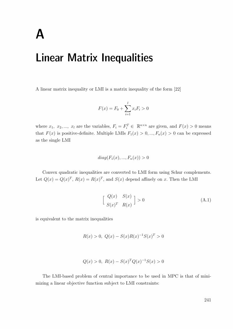
A
Linear Matrix Inequalities
A linear matrix inequality or LMI is a matrix inequality of the form [22]
F (x) = F0 +l∑
i=1
xiFi > 0
where x1, x2, ..., xl are the variables, Fi = F Ti ∈ Rn×n are given, and F (x) > 0 means
that F (x) is positive-definite. Multiple LMIs F1(x) > 0, ..., Fn(x) > 0 can be expressed
as the single LMI
diag(F1(x), ..., Fn(x)) > 0
Convex quadratic inequalities are converted to LMI form using Schur complements.
Let Q(x) = Q(x)T , R(x) = R(x)T , and S(x) depend affinely on x. Then the LMI
[ Q(x) S(x)
S(x)T R(x)
]> 0 (A.1)
is equivalent to the matrix inequalities
R(x) > 0, Q(x) − S(x)R(x)−1S(x)T > 0
Q(x) > 0, R(x) − S(x)TQ(x)−1S(x) > 0
The LMI-based problem of central importance to be used in MPC is that of mini-
mizing a linear objective function subject to LMI constraints:
241

Appendix A. Linear Matrix Inequalities
minimize cTx
subject to F (x) > 0(A.2)
where F is a symmetric matrix that depends affinely on the optimization variable x, and
c is a real vector of appropriate size.
A.1 S-procedure
Let F0, . . . , Fp be quadratic functions of the variable ζ ∈ Rn [22]:
Fi(ζ) ζTTiζ + 2uTi ζ + vi, i = 0, . . . , p
where Ti = T Ti . Consider the following condition on F0, . . . , Fp:
F0(ζ) ≥ 0 ∀ζ s.t. Fi(ζ) ≥ 0, i = 1, . . . , p (A.3)
Obviously if there exits τ1 ≥ 0, . . . , τp ≥ 0 such that for all ζ,
F0(ζ) −p∑i=1
τiFi(ζ) ≥ 0 (A.4)
then (A.3) holds (S-procedure). It is a nontrivial fact that when p = 1, the converse
holds, provided that there is some ζ0 such that F1(ζ0) > 0.
Note that (A.4) can be written as
⎡⎣ T0 u0
uT0 v0
⎤⎦−
p∑i=1
τi
⎡⎣ Ti ui
uTi vi
⎤⎦ ≥ 0
S − procedure can be varied in order to involve quadratic forms and strict inequali-
ties. Let T0, . . . , Tp ∈ Rn×n be symmetric matrices. Consider the following condition on
T0, . . . , Tp:
ζTT0ζ > 0 ∀ζ = 0 s.t. ζTTiζ ≥ 0, i = 1, . . . , p (A.5)
It is obvious that if there exists
242

A.1 S-procedure
τ1 ≥ 0, . . . , τp ≥ 0 | T0 −p∑i=1
τiTi > 0
then (A.5) holds. It is a non trivial fact that when p = 1, the converse holds, provided
that there is some ζ0 such that ζT0 Tiζ0 > 0.
243