Embed Size (px)
Citation preview
. ___---- --
NASA Contmctor Report 3592
Tensile Stress-Strain Behavior of Graphite/ Epoxy Laminates
D. P. Garber
CONTRACT NASl-16000 AUGUST 1982
NASA CR 3592 c-1 >
https://ntrs.nasa.gov/search.jsp?R=19820022692 2018-06-15T19:13:43+00:00Z
SUMMARY
The tensile stress-strain behavior of a variety of graphite/epoxy laminates
was examined. Longitudinal and transverse specimens from eleven different layups
were monotonically loaded in tension to failure. Ultimate strength, ultimate
strain, and stress-strain curves were obtained from four replicate tests in each
case, Polynominal equations were fitted by the method of least squares to the
stress-strain data to determine average curves. Values of Young's modulus and
Poisson's ratio, derived from polynomial coefficients, were compared with laminate
analysis results.
While the polynomials appeared to accurately fit the stress-strain data in.
most cases, the use of polynomial coefficients to calculate elastic moduli appeared
to be of questionable value in cases involving sharp changes in the slope of the
stress-strain data or extensive scatter.
I
TABLE OF CONTENTS
Page
INTRODUCTION . . . . . . . . . . . . . . . . . . . . . . . . . . . . . . 1
SYMBOLS ................................. 2
EXPERIMENTAL PROCEDURES ......................... 3
DATAANALYSIS .............................. 4
DISCUSSION OF RESULTS .......................... 7
SUMMARY OF RESULTS ........................... 15
REFERENCES ............................... 17
TABLES ................................ . 18
FIGURES ................................. 39
ii
INTRODUCTION
The study of the tensile fracture of continuous fiber laminated composites can
be roughly divided into two categories: unnotched fracture and notched fracture.
In unnotched composites, failure appears to be controlled in part by the compli-
cated stress states occurring at the free edges. The edge stresses are determined
not only by the presence of different ply orientations, but by the order of the ply
orientations or stacking sequence. Failure models which are used to predict
unnotched failure require some information about the behavior of the constituent
laminae. Simple models need only elastic constants while more sophisticated models
might use the nonlinear response of the individual laminae. In the fracture of
notched composites, notch geometry plays a predominant role. In this category
stacking sequence is of considerably less importance than flaw shape in determining
failure (ref. 1). Notched composite failure models generally require the laminate
unnotched strength and elastic constants.
The primary objective of this study was to provide elastic constants and
unnotched strengths for analysis of the notched strengths of a wide variety of
graphite/epoxy laminates. In order to achieve this objective, longitudinal and
transverse specimens of each layup were monotonically loaded in tension to
failure. The use of polynomial equations to model the stress-strain curves which
were generated was also explored. Elastic constants were obtained from the
polynomial coefficients and compared with laminate analysis results to evaluate the
effectiveness of this approach.
1
SYMBOLS
a. lxx
aixy
EX
(Etan) x
El
E2
F tu
G12
R2xx
R2xy
vf
E X
“Y
%U
vxY
(Vtan) xy
V 12
ith coefficient of the longitudinal strain polynomial, (GPa)-i
ith coefficient of the transverse strain polynomial, (GPa)-i
Young's modulus, GPa
tangent modulus, GPa
lamina Young's modulus, fiber direction, GPa
lamina Young's modulus, perpendicular to fibers, GPa
ultimate tensile strength, MPa
lamina shear modulus, GPa
adjusted R2 statistic of the longitudinal strain polynomial
adjusted R2 statistic of the transverse strain polynomial
fiber volume fraction
longitudinal strain
transverse strain
ultimate tensile strain
Poisson's ratio
tangent Poisson's ratio
lamina Poisson's ratio
u X
longitudinal stress, MPa
EXPERIMENTAL PROCEDURES
Material and Specimens
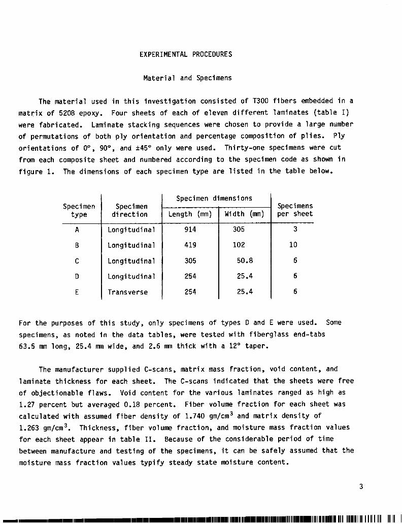
The material used in this investigation consisted of T300 fibers embedded in a
matrix of 5208 epoxy. Four sheets of each of eleven different laminates (table I)
were fabricated. Laminate stacking sequences were chosen to provide a large number
of permutations of both ply orientation and percentage composition of plies. Ply
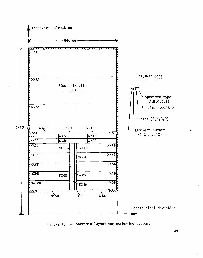
orientations of O", 90°, and 245" only were used. Thirty-one specimens were cut
from each composite sheet and numbered according to the specimen code as shown in
figure 1. The dimensions of each specimen type are listed in the table below.
Specimen Specimen type direction
A Longitudinal
B Longitudinal
C Longitudinal
D Longitudinal
E Transverse
Specimen dimensions
Length (mm) Width (mm)
914 305
419 102
305 50.8
254 25.4
254 25.4
1 Specimens per sheet
3
10
6
6
6
For the purposes of this study, only specimens of types D and E were used. Some
specimens, as noted in the data tables, were tested with fiberglass end-tabs
63.5 nm long, 25.4 mn wide, and 2.6 mn thick with a 12" taper.
The manufacturer supplied C-scans, matrix mass fraction, void content, and
laminate thickness for each sheet. The C-scans indicated that the sheets were free
of objectionable flaws. Void content for the various laminates ranged as high as
1.27 percent but averaged 0.18 percent. Fiber volume fraction for each sheet was
calculated with assumed fiber density of 1.740 gm/cm3 and matrix density of
1.263 gm/cm3. Thickness, fiber volume fraction, and moisture mass fraction values
for each sheet appear in table II. Because of the considerable period of time
between manufacture and testing of the specimens, it can be safely assumed that the
moisture mass fraction values typify steady state moisture content.
Test Procedure and Equipment
Specimens were tested in a single channel, closed loop, servo controlled,
hydraulically activated testing machine equipped with hydraulic grips. Cellulose
acetate shims 1.5 mn thick were placed between the specimen and grip faces, and
gripping pressure was adjusted to prevent damage to the ends of the specimens. The
controller was set to operate with feedback from the load cell and the command
.signal was provided by an external function generator set on ranp mode. The ramp
rate was chosen so as to strain the specimens at approximately 1O-4 mn/mm/second.
Strains were measured by bonded foil strain gages with 3.2 rrm gage length.
One longitudinal and one transverse gage were mounted on each side of the
specimen. The longitudinal gages were wired in series and connected so as to
constitute one arm of a Wheatstone bridge. The transverse gages were similarly
connected to a separate bridge.
Data for each test were sampled and recorded by a digital data acquisition
system (ref. 2). Analogue voltage signals from the load cell conditioner, strain
gage circuits, and a peak meter connected to the load cell conditioner were
sequentially sampled at fixed intervals by a scanner. An integrating digital
voltmeter converted the analogue inputs, and the data were recorded on an
incremental magnetic tape recorder and a digital paper tape printer.
DATA ANALYSIS
Data Reduction
Information recorded on magnetic tape by the data acquisition system was
copied onto a computer file and processed by a data reduction program. Because the
analogue signals varied with time but were sampled sequentially rather than instan-
taneously, data within a scan were interpolated to coincide in time. The linear
interpolation was considered to be sufficiently accurate due to the linear nature
of the command signal supplied to the testing machine controller. All data
recorded prior to loading and after specimen failure were automatically eliminated
by the data reduction program. Load was converted to stress using a
4
cross-sectional area based on an assumed ply thickness of 0.14 mn and the measured
specimen width. The ultimate tensile strength was determined from the maximum
value recorded on the peak meter channel.
Curve Fitting
The stress and strain data were fit to polynomial equations of the form:
Ex = aOxx + alXXaX + 82xX0x2 + l + anxxQxn
ey = aoxy + a1xycJx + a2xyux 2, . . . + anxyuxn
by Gauss' least-squared-error method. The x and y subscripts refer, respec-
tively, to the directions parallel with and perpendicular to the applied load. To
satisfy the requirement that the stress-strain curves have inflection points at
zero load, the coefficients a2xx and a2xy were set to zero prior to initiating
the least squares procedure. The adjusted R2 statistic (ref. 3) was calculated for
polynomials of various orders to provide a quantitative measure for deciding which
order to use. It was decided that a fourth order polynomial gave the best fit with
the fewest parameters. The stress-strain parameters and the associated adjusted R2
statistics for each specimen appear in table III.
Figure 2 shows the stress-strain curve for specimen 2A2E with the data plotted
as symbols and the polynomials drawn as solid lines to give an example of the
accuracy of the method. The rest of the specimens are plotted in groups according
to stacking sequence (fig. 3-27). Data for each specimen are distinguished by the
use of different symbols, and the polynomial curves in each case were determined by
averaging the coefficients of the polynomials fit to each specimen (see table III).
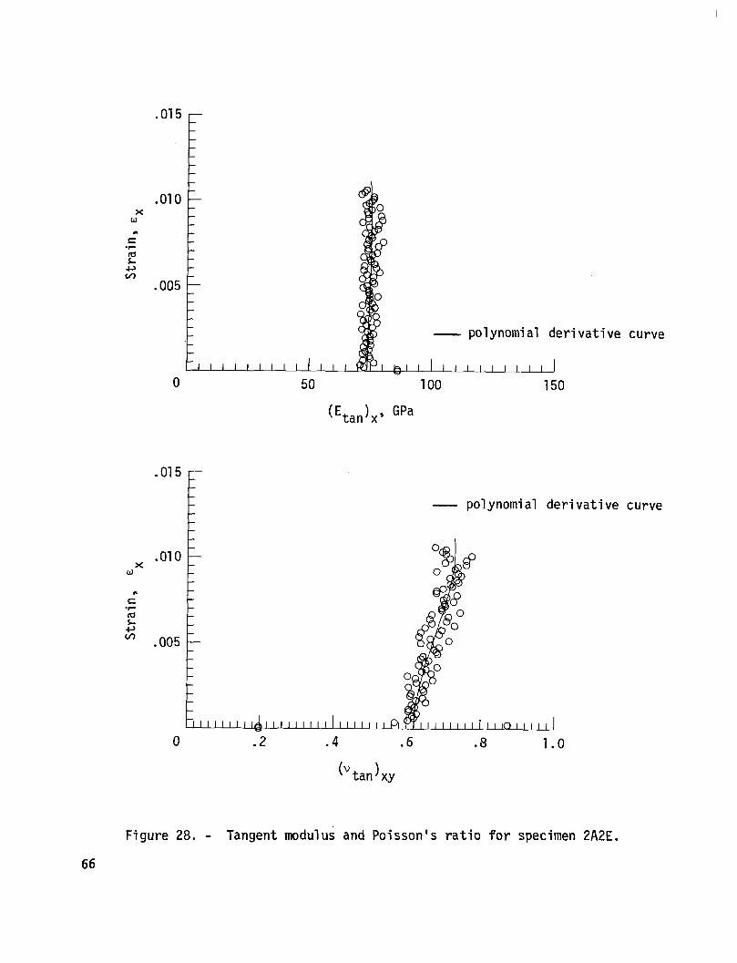
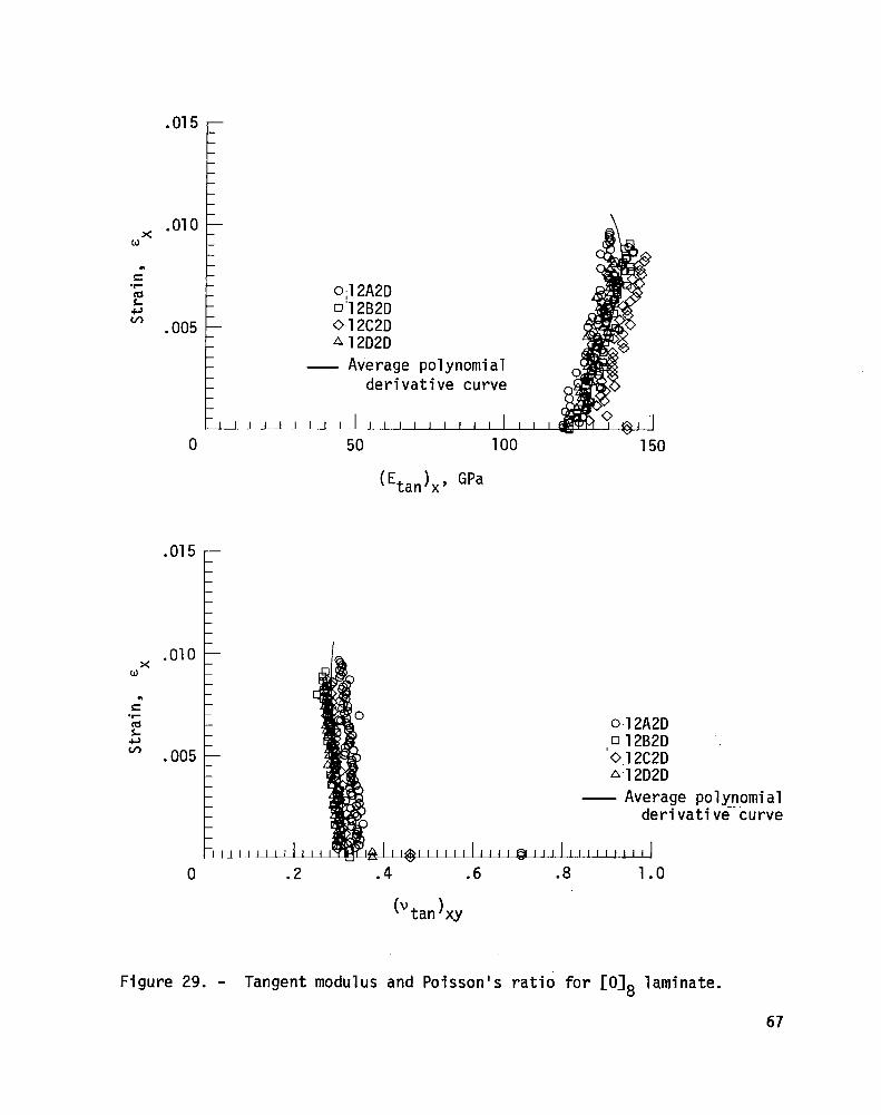
Figure 28 shows the tangent modulus and tangent Poisson's ratio plotted
against longitudinal strain for specimen 2A2E. The polynomial derivative curves:
and (u tan xy = )
are drawn as solid lines while the data, calculated using a first-order backward
difference method, are plotted as symbols. The rest of the specimens are plotted
in groups according to stacking sequence (fig. 29-53). Data for each specimen are
distinguished by the use of different symbols as before and the polynomial deriva-
tive curves in each case are again determined by averaging the coefficients of the
individual derivatives.
Laminate tensile elastic constants were determined from the polynomial
equations which were fit to the digital data. Young's modulus was derived from the
longitudinal strain polynomial:
-1 = alxx
and Poisson's ratio was derived from the longitudinal and transverse strain
polynomials:
vxY = {- (~yl(gg} =-a
uX =o lxy’alxx
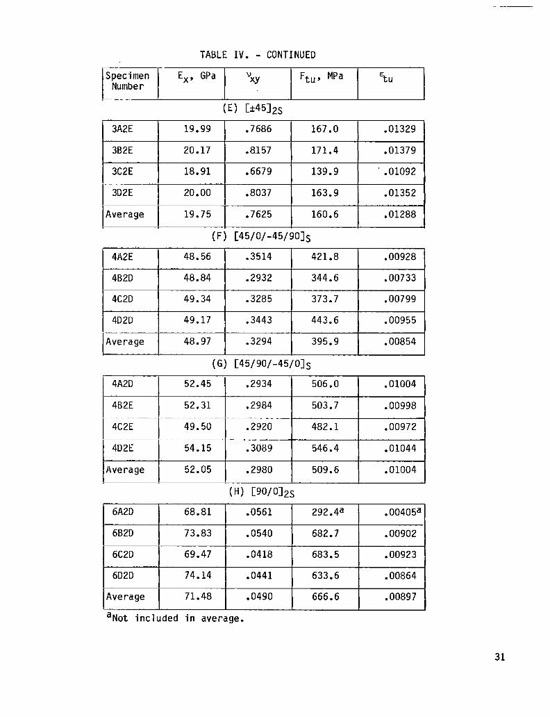
These constants along with the unnotched tensile strength and ultimate strain for
each specimen appear in table IV.
Lamina elastic constants required for a laminate analysis (ref. 4) were
calculated using laminate elastic values (from table III) for [O]s, [901a, and
[+45]231aminates. The lamina shear modulus was determined using Rosen's method
(ref. 5). The constants used in the laminate analysis appear in the table below.
El 1 129.4 GPa
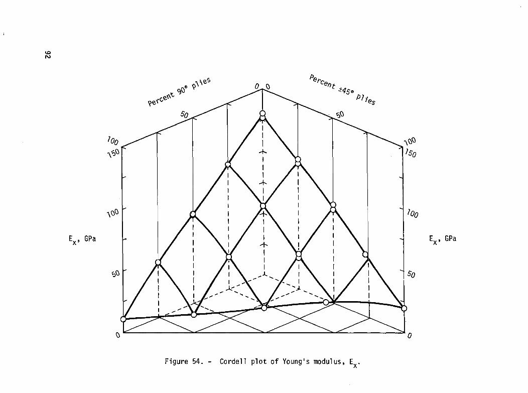
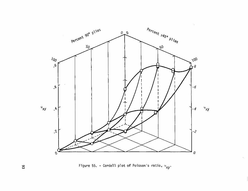
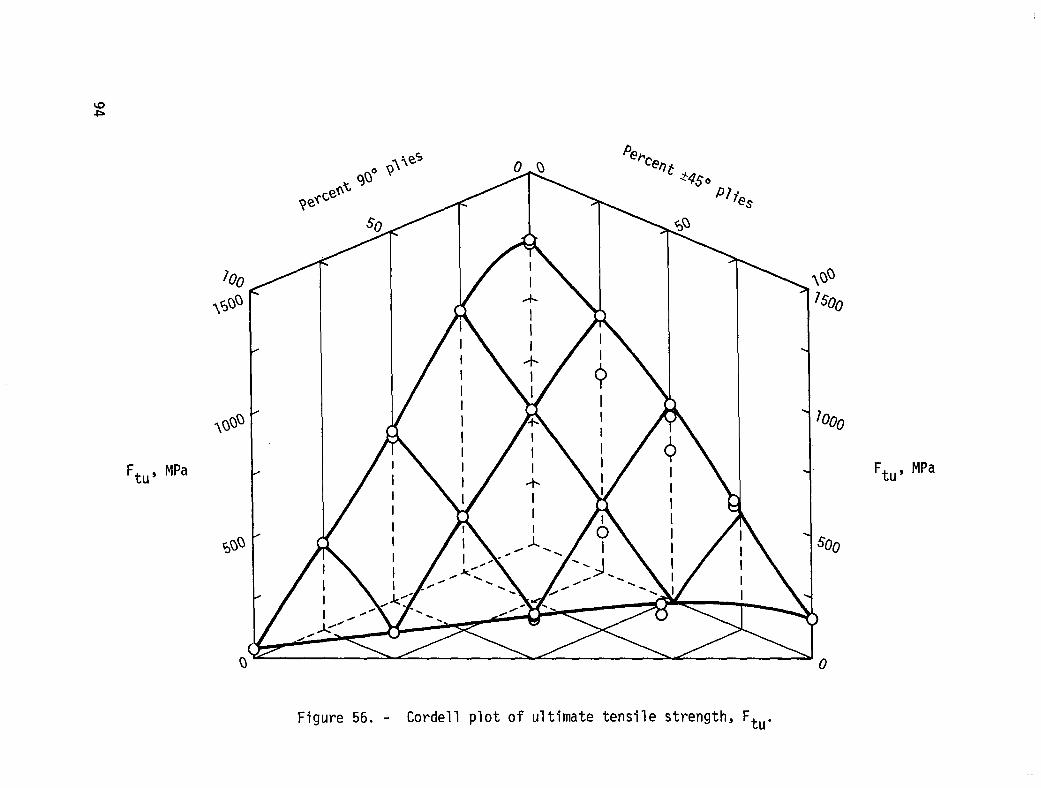
Experimental and theoretical values of Young's modulus and Poisson's ratio
appear in table V for comparison purposes. Cordell plots (ref. 6) have been drawn
for the experimental values of Young's modulus (fig. 54), Poisson's ratio (fig.
55), and the unnotched tensile strength (fig. 56). A fourth order polynomial
surface has been determined for each plot using Gauss' least-squares method to
provide an aid for visualizing the material behavior. Data are plotted as symbols
and the polynomials are plotted as lines of constant ply percentage.
DISCUSSION OF RESULTS
Stress-Strain Curves
Polynomials determined by the least squares method are used to represent the
stress-strain data for several reasons. The primary reason is that the entire
curve can be modeled with only a few parameters. Polynomials from several speci-
mens of the same layup can be averaged quite simply by averaging coefficients,
thereby also simplifying the determination of average elastic moduli. The calcula-
tion of the parameters involves no user bias beyond the selection of the highest
order, and statistics (such as the adjusted R2) are available as indicators of the
accuracy of fit to guide in selecting the highest order. Derivatives are easy to
calculate and the entire procedure can be automated on a digital computer.
Residual plots are desirable for determining whether differences between data and
the polynomial fit are systematic or random. It was decided, however, that the
nature of the stress-strain behavior would yield systematic differences regardless
of polynomial order so the adjusted R2 statistic alone was used. Fourth order
curves were considered to best meet the criterion of maximizing the adjusted R2
while minimizing the number of parameters. Figure 2 shows just one example of
polynomial fits to longitudinal and transverse stress-strain data.
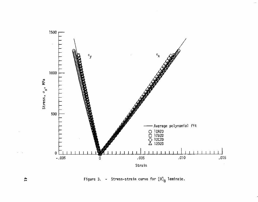
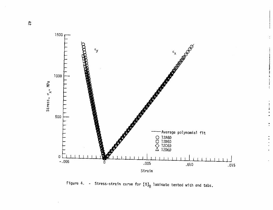
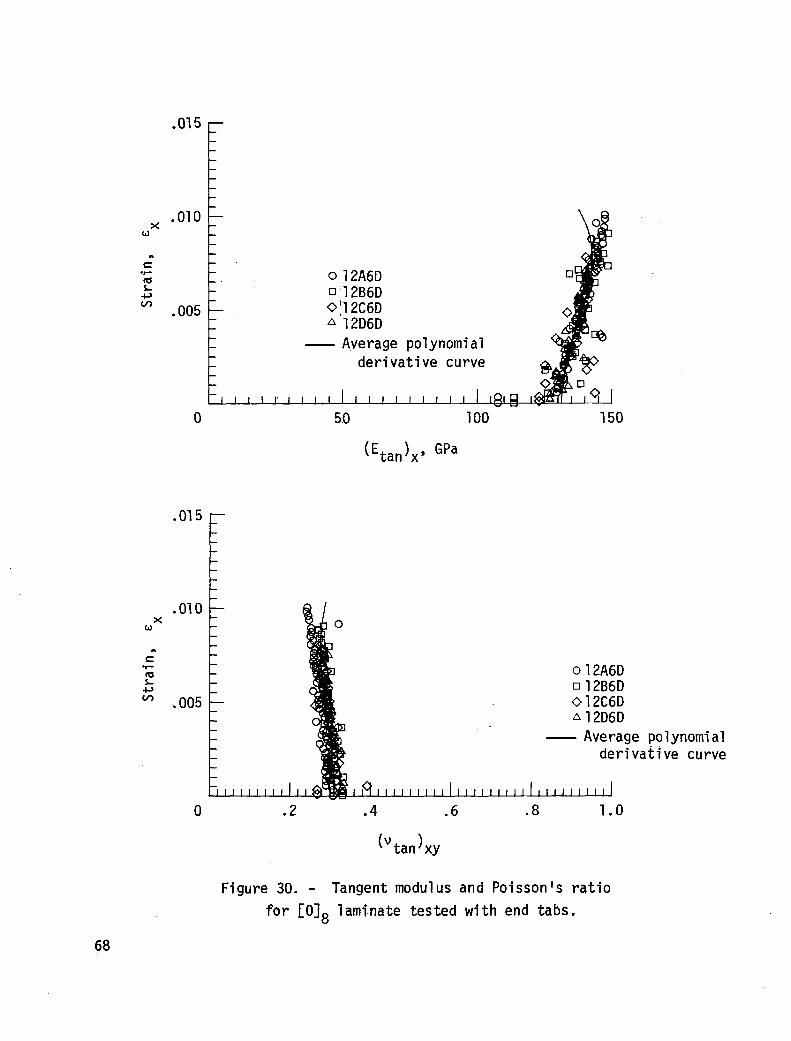
Data and curves for [O]s specimens are shown in figure 3 for tests performed
on un-tabbed specimens and in figure 4 for tests performed on end-tabbed speci-
mens. The low failure strains observed in tests performed without tabs indicated
that the gripping method might have contributed to early failure. Tests run on
specimens with tapered tabs showed no significant differences in ultimate stress or
strain or in polynomial coefficients. One study (ref. 7) has shown that tapered
7
tabs can debond and contribute to early failure. In the case of the [O]s laminate,
the tabs debonded from the specimen but did not appear to affect the failure mode.
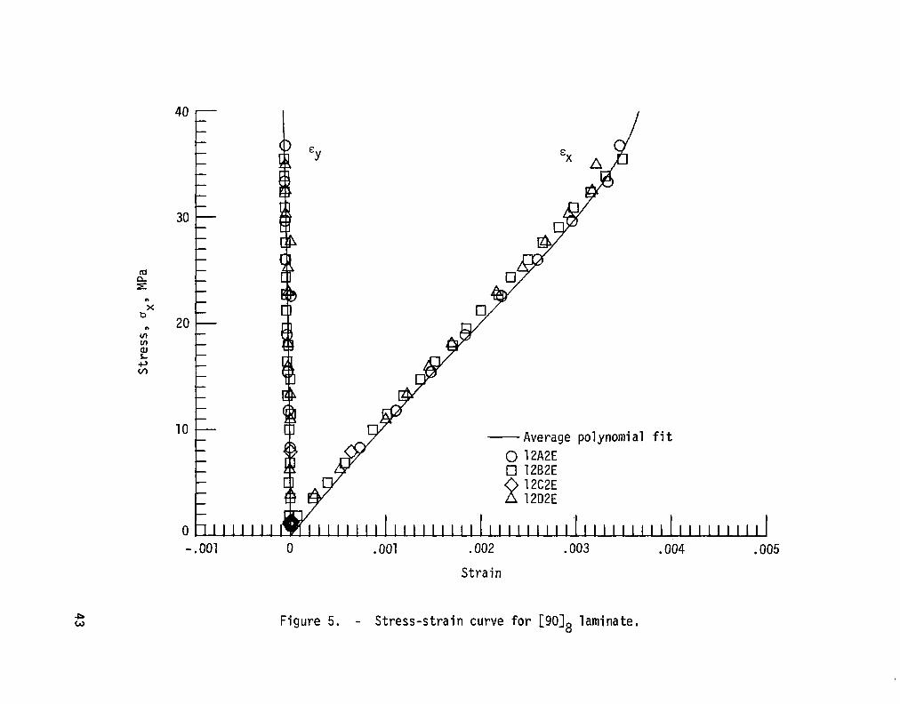
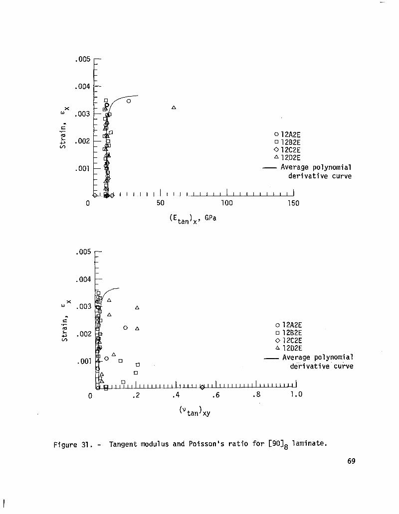
Figure 5 shows the results for tests of the [9O]s laminate. Each specimen
failed neatl, y at a grip edge. While the curves appear to fit the data very well,
examination of the adjusted R2 statistics in table III reveals that transverse
strain data is not fit well. This is due to a very poor signal-to-noise ratio
resulting fr om the extremely small strain levels. The data may also be biased
because the effect of transverse sensitivity was not taken into account. The
transverse sensitivity factor was not recorded when the gages were applied. Curves
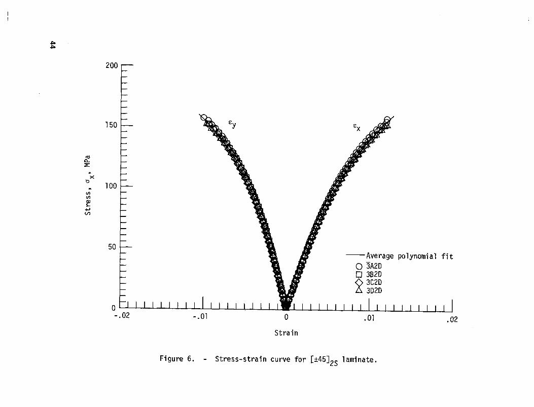
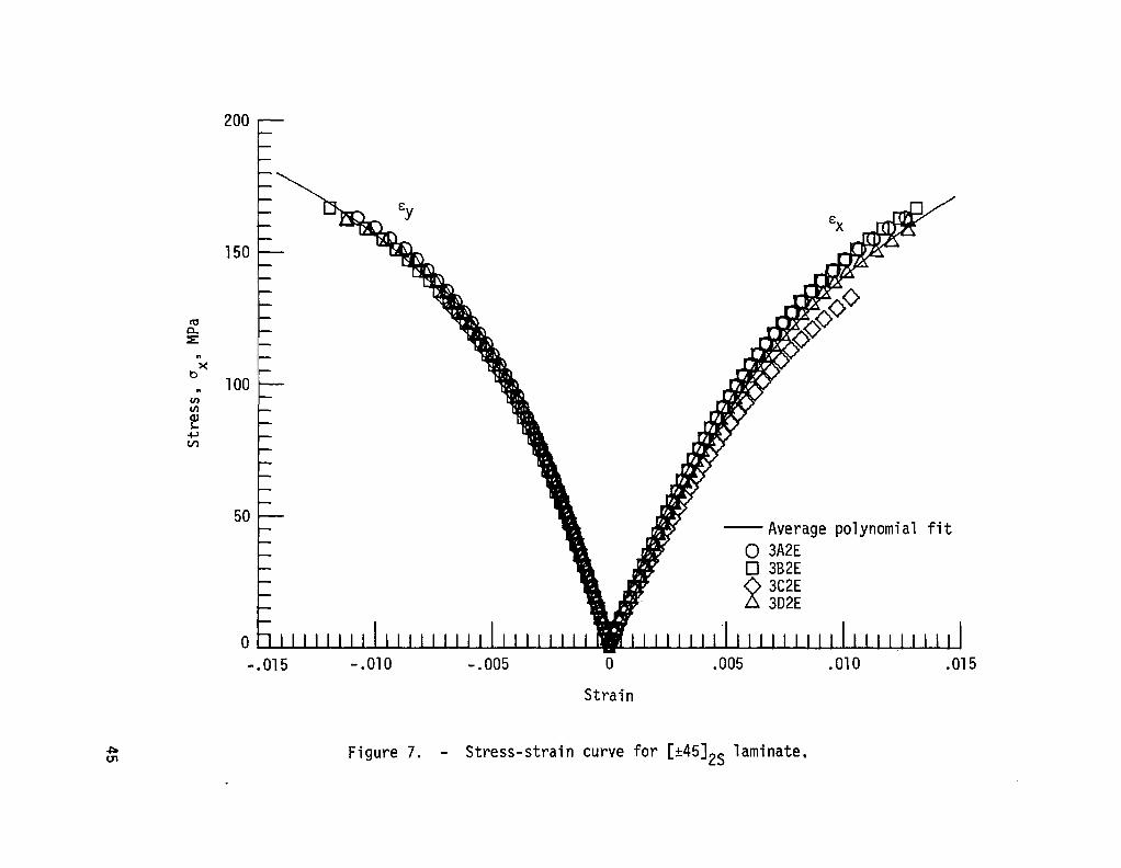
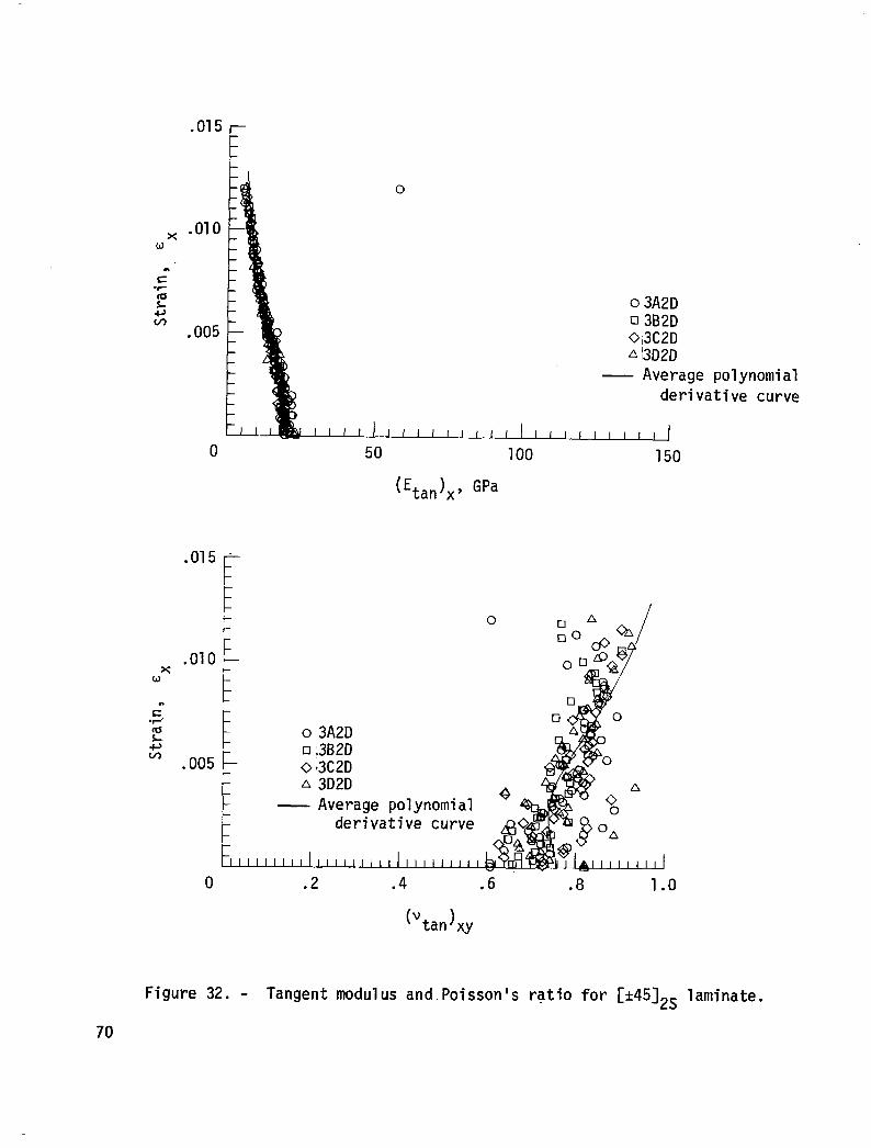
for the [-+45],S laminate shown in figures 6 and 7 are extremely nonlinear but
seem to be well fit by the polynomials.
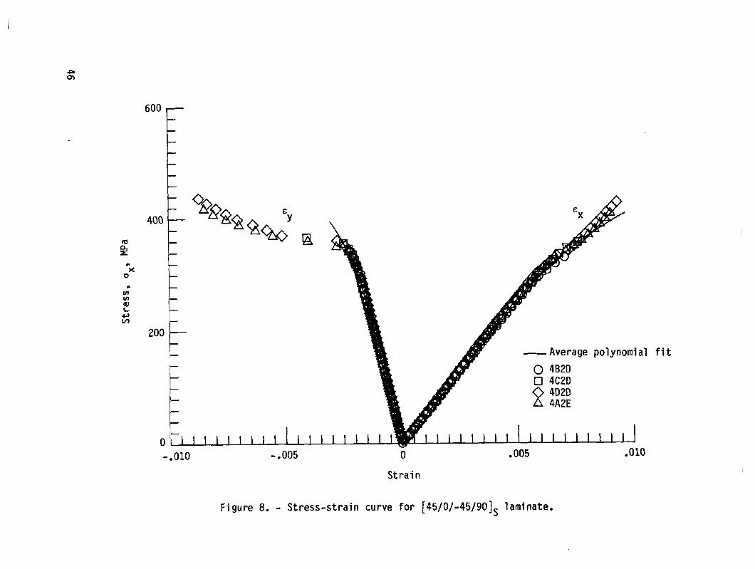
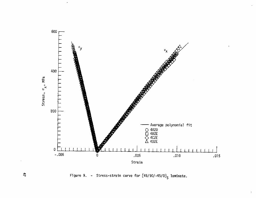
The results of tests on so-called quasi-isotropic laminates, [45/O/-45/9O]S
and [45/90/-45/O]S, are shown in figures 8 and 9. The laminate with 90' plies in
the center exhibits significantly lower failure stresses and strains than the
laminate with O" plies in the center, and shows distinctly nonlinear behavior prior
to failure. Examination of failed specimens revealed extensive delamination of the
-45/90 interfaces for specimens with 90" plies at the center while specimens with
0' plies in the center showed only minor delamination at one 45/90 interface.
Approximate interlaminar stresses were calculated using the method of Pipes and
Pagan0 (ref. 8). Calculations for the [45/O/-45/9O]S laminate show very high
tensile stresses normal to the interface between the -45" and 90" plies.
Calculations for the [45/90/-45/O]S laminate show compressive stresses at every
interface except for the 45/90, which has a very slight tensile stress. The
nonlinear behavior evident in figure 8 is due to extensive delamination growth
which contributed to the low failure stress. In order to obtain more accurate
elastic constants, polynomials were fit only to stress-strain data recorded prior
to the onset of delamination for the [45/O/-45/9O]S laminate.
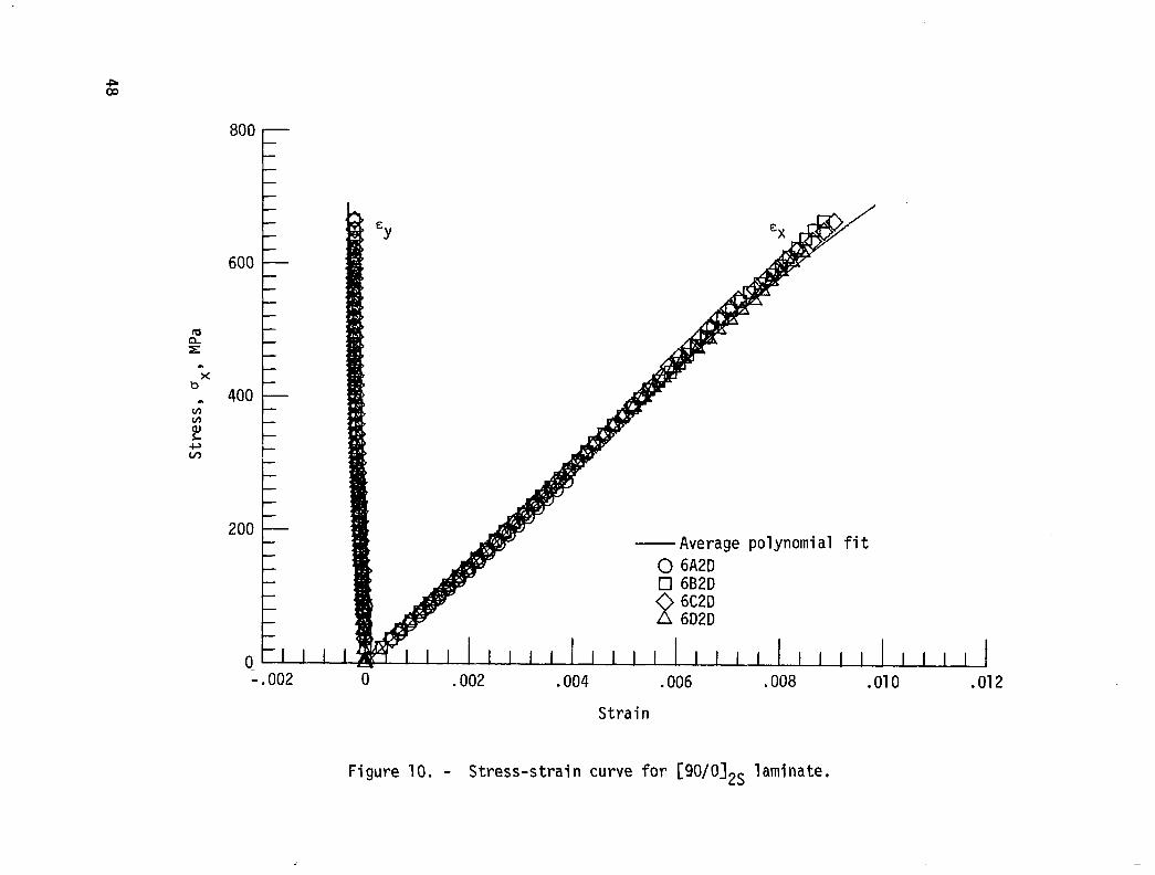
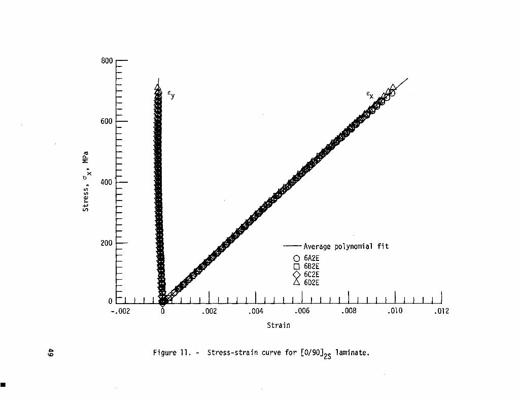
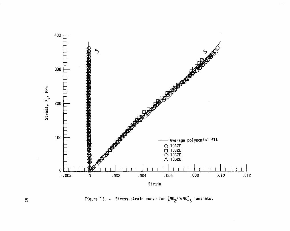
Figures lo-13 show the stress-strain behavior of [90/O12S, [O/90]2S,
[02/9O/O]S, and [902/O/90]S laminates. The transverse strain is small in each
case bacause of the presence of 90" plies and absence of +45' plies. Only one
laminate, [902/O/90]S, figure 13, shows distinct nonlinearity in the longitudinal
strain. All of the specimens of these layups broke in the test section in a nearly
straight line. Specimens of the [0,/9O/O]S layup had very small delaminated
areas at the break.
8
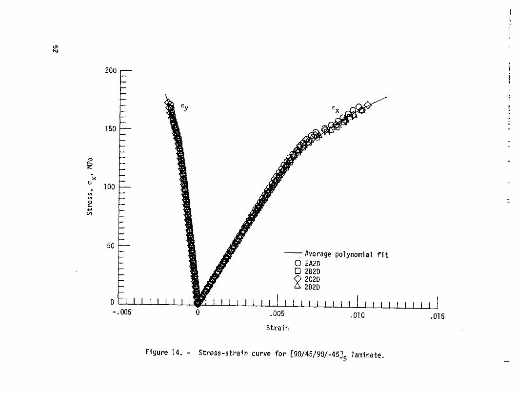
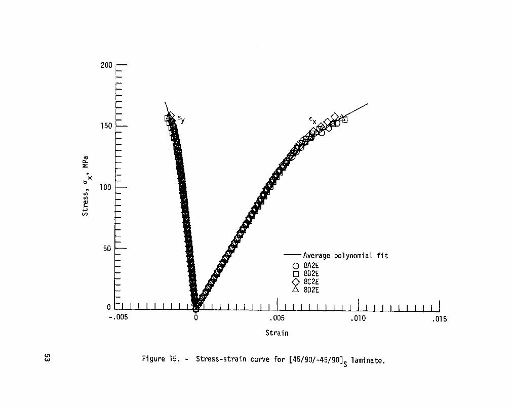
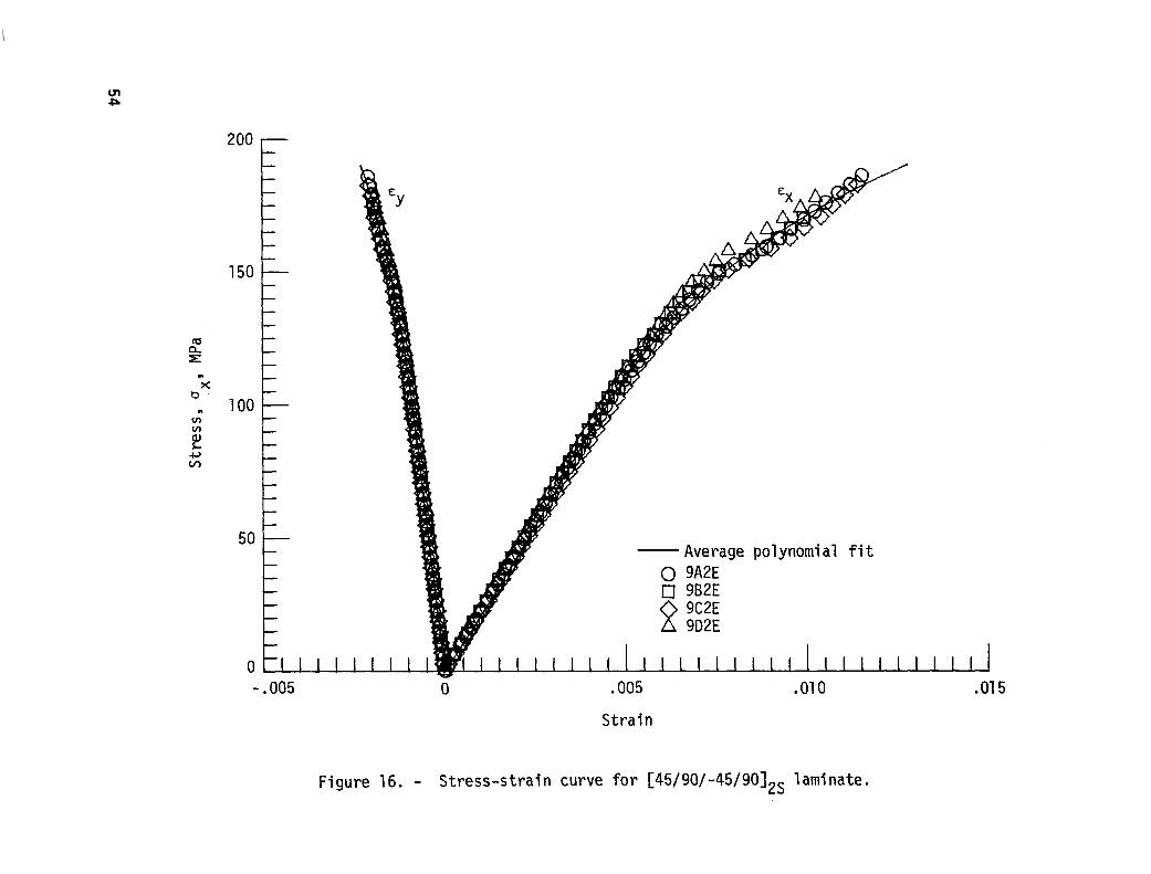
Stress-strain curves for [90/45/90/-45]S, [45/90/-45/9O]S, and
[45/90/-45/9012S laminates shown in figures 14, 15, and 16 exhibit nearly
identical behavior. Failure surfaces for all three laminates appear the same with
straight breaks in 90" plies and pull out in 45" plies.
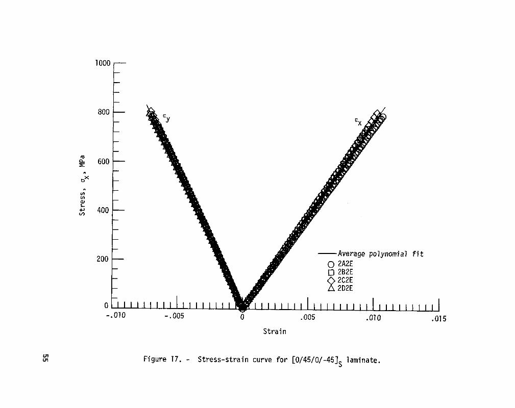
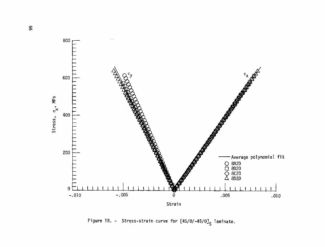
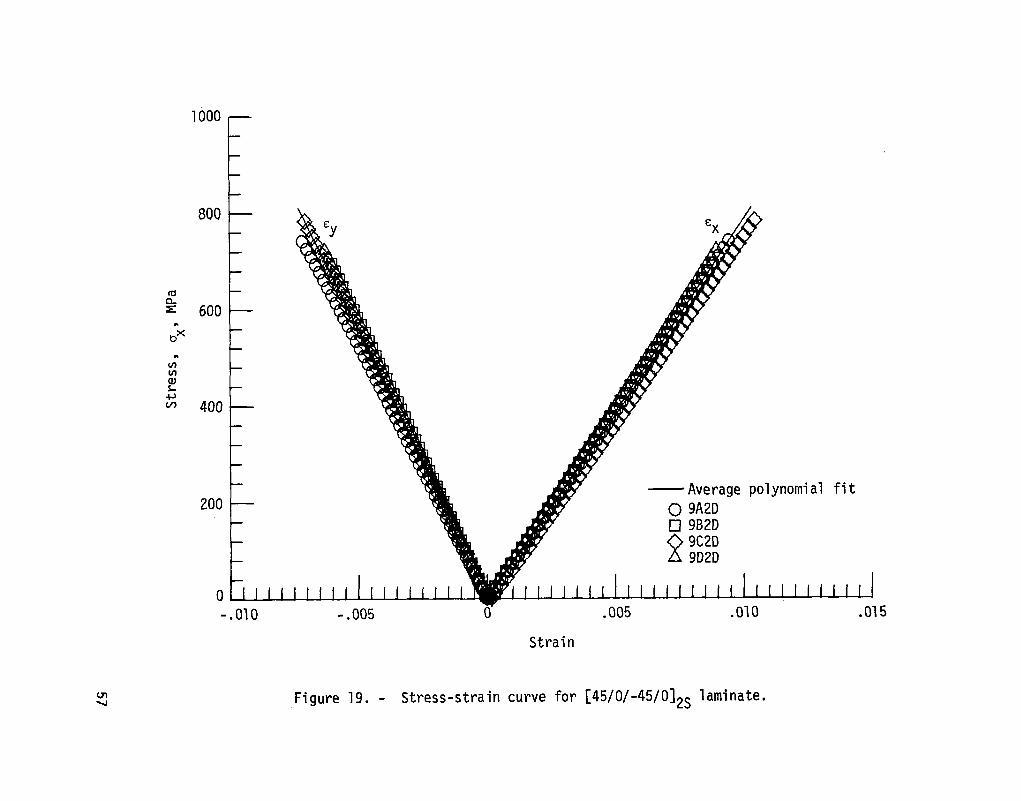
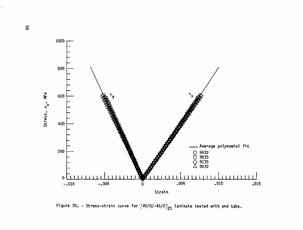
Figures 17-20 show the behavior of [O/45/0/-45]S, [45/O/-45/O]S, and
[45/O/-45/O]2S laminates and the [45/O/-45/O]2S laminate with tapered end
tabs. While all four sets of curves appear to have identical slopes, each laminate
failed at a different strain. Interlaminar normal stresses appear to be the
distinguishing factor. The Pipes and Pagan0 approximation (ref. 8) indicates that
the interlaminar normal stresses in the laminate with the highest failure strain,
[O/45/0/-45]S, are compressive. The same method indicates that normal stresses
in the laminate with the lowest failure strain, [45/O/-45/O]S, are tensile. The
interlaminar stresses in the [45/O/-45/O],S laminate are intermediate in size,
but postmortem examination of the end-tabbed specimens revealed that the end-tabs,
instead of debonding, pulled the outer plies completely free in- the region at the
edge of the tab. All failures of the end-tabbed specimens occurred very near the
tabs. Postmortem examinations revealed that delaminations were present, to some
extent, in the failed region of every specimen in this group. There is no clear
evidence, however, to indicate whether the delaminations contributed to or were
caused by failure of the specimens.
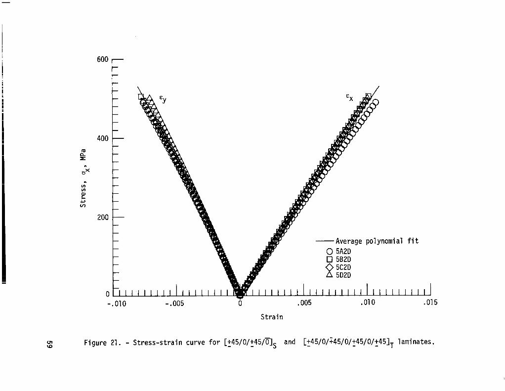
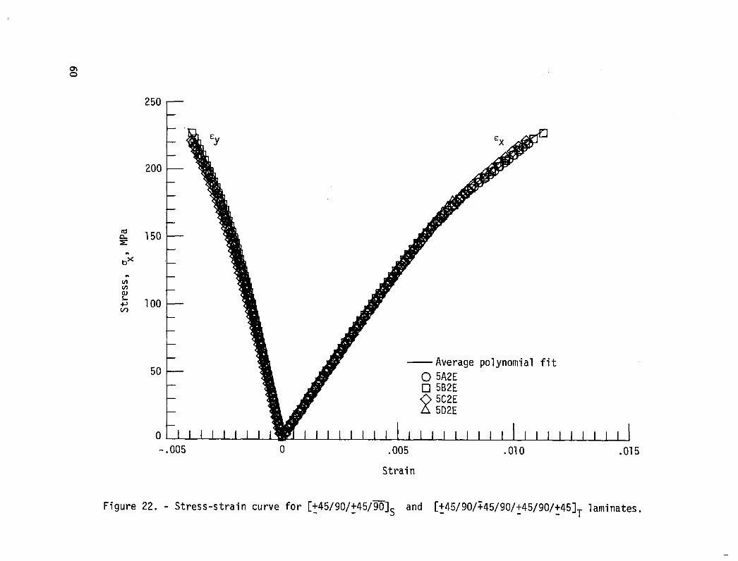
Figures 21 and 22 show the behavior of the [+45/0/*45/01S,
['45/0/r45/0/?45/0/+45]T, [+45/90/+45/9O]S, and [+45/90/745/90/+45/90/+45]T
laminates. Although layup errors occurred for this group of laminates (see table
I), there appear to be no significant differences in behavior between the correctly
and incorrectly stacked laminates. Specimen 5D2E failed at a very low stress and
strain, but no conclusions may be drawn from a single test. The failure surface
shape did not appear to depend on the stacking error.
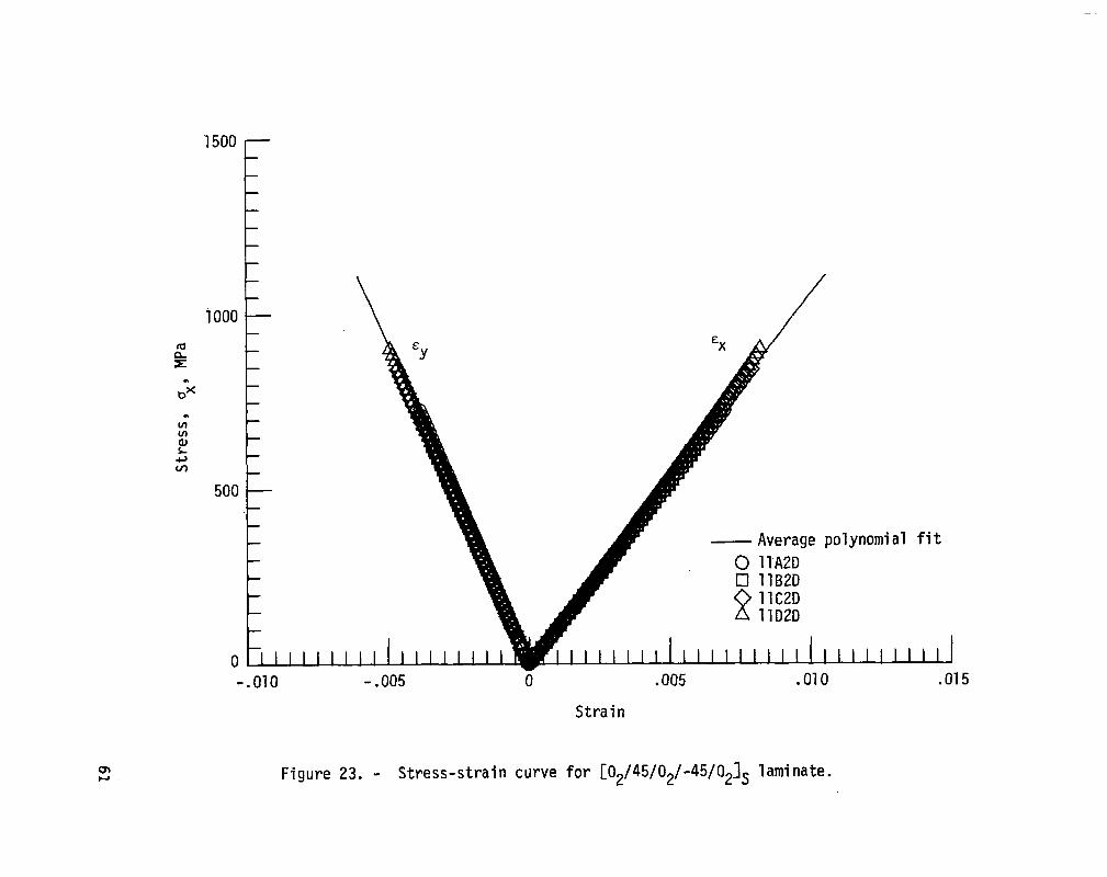
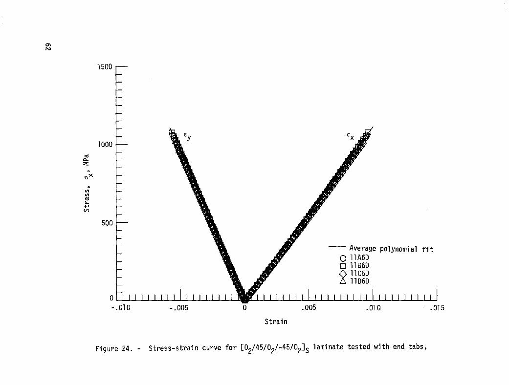
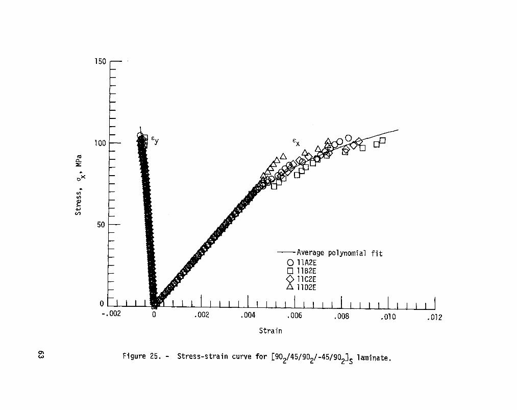
Stress-Strain behavior Of the [02/45/O,/-45/02]S laminate iS shown in figure
23. All four specimens failed in the grip. Figure 24 shows the behavior of the
same laminate tested with end tabs. In this case end tabs solved the gripping
problem; none of the specimens failed in the grips and there was substantial
improvement in the failure stress and strain. The behavior of the
[902/45/902/-45/902]S laminate is shown in figure 25. Although there is little
difference between the failure stresses of the specimens, the range of failure
strains is quite large. Since significant differences between specimens appear
only above a strain of 0.004, approximately the ultimate strain of the [90]s
laminate, it would seem that damage to the 90" plies is responsible.
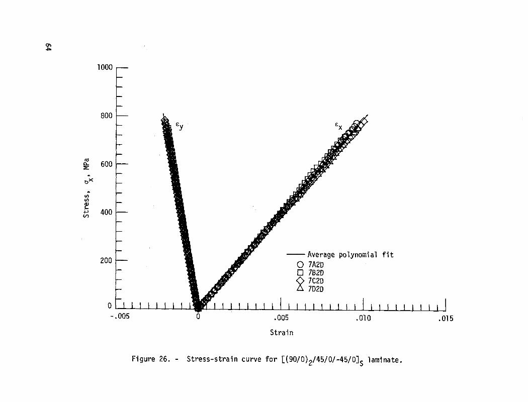
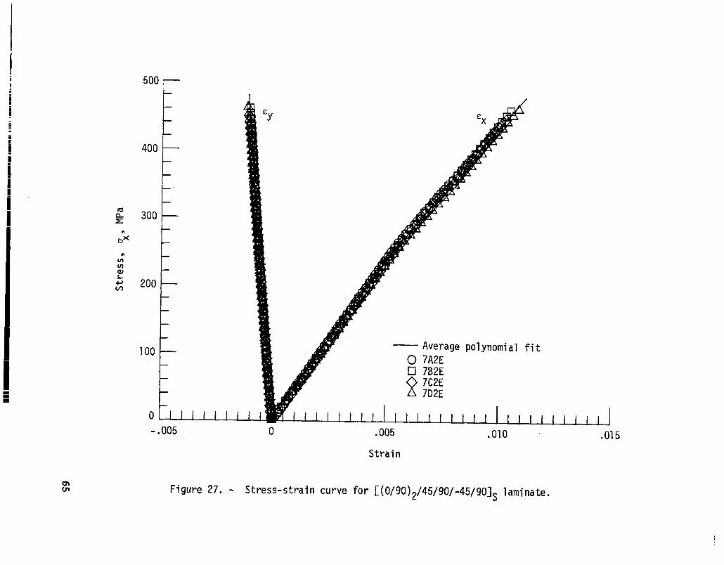
Stress-strain curves for [(90/0)2/45/O/-45/O& and [(O/90)2/45/90/-45/9O]S
laminates appear in figures 26 and 27. There is very little variation in ultimate
stress, ultimate strain, or the appearance of the stress-strain curve between
replicate tests for either laminate configuration.
Stiffness and Poisson's Ratio Curves
In order to display the manner in which stiffness and Poisson's ratio change
with increasing strain, derivatives of the least squares polynomials are plotted.
Figure 28 shows the results for specimen 2A2E. The symbols in that figure and
subsequent figures represent slopes between successive pairs of scans determined by
a first-order backward difference scheme. They show both the degree of agreement
between data and polynomial derivatives, and the extent to which slight scatter in
the raw data can be magnified by a simple finite difference procedure. The least
squares method, it should be noted, does not involve fitting derivatives.
Polynomial coefficients are determined only by minimizing discrepancies between
data and the curve. The polynomial derivative curves should, therefore, be
considered with this limitation in mind.
Tangent modulus and Poisson's ratio curves for the unidirectional laminates
appear in figures 29-31. The [O]s laminate stiffness increases significantly with
increasing strain while Poisson's ratio drops correspondingly. It appears from the
data in figures 29 and 30 that even though the stiffness of the [O]a laminate has
non-zero slope at zero strain, the polynomial adequately models the stiffness of
the [Ola laminate. The results for the [9OJa laminate (fig. 31) indicate a
constant stiffness over nearly the entire strain range, but the lack of transverse
strain sensitivity correction makes the plot of Poisson's ratio suspect. Plots of
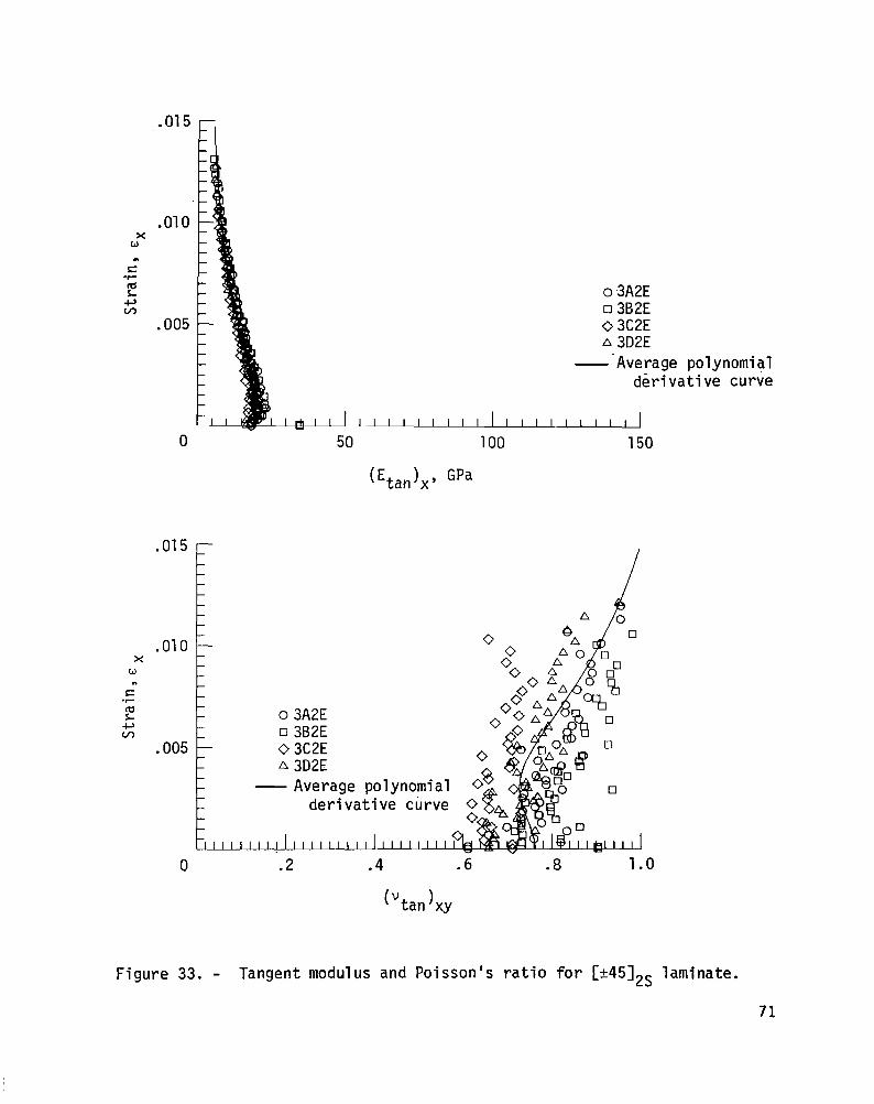
the [*45],S laminate behavior in figures 32 and 33 show stiffness decreasing with
increasing strain, while Poisson's ratio increases to nearly 1. The Poisson's
ratio plots of the [+45]zS laminate show the value of using polynomials to
10 ,
ameliorate the problem of data scatter caused by digital data acquisition.
Although the curve-fittin.g method used is not perfect, it appears to work well for
the [OJa, [9O]a, and [+45],3 laminate stress-strain data from which the lamina
elastic properties are derived.
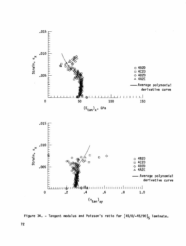
The disparity between the responses of the two different quasi-isotropic
laminates mentioned previously is apparent in the plots of figures 34 and 35. The
[45/O/-45/9015 laminate exhibits an abrupt stiffness drop at 0.004 strain. At
that strain level scatter increases substantially. The ultimate strain of the
[9O]a laminate (table V) is about 0.0036. This suggests that splitting in the 90"
plies may be responsible for the decrease of the laminate stiffness and the scatter
in the data. An edge replicate obtained from one specimen indicates that cracks
were present in the 90° plies at a strain as low as 0.0038. Also, an edge
replicate indicated that delaminations were present at a strain as low as 0.0045.
Although a report by O'Brien, et.al. (ref. 9) suggests that matrix cracking in
off-axis plies contributes relatively little to laminate stiffness loss, it should
be noted that small laminate stiffness changes are more pronounced when the tangent
to the stress-strain curve, rather than the secant, is plotted. The relationship
between tangent modulus and secant modulus is:
E E tan = set
while changes in the tangent modulus are related to changes in the secant modulus
by:
$(Etan)= 2 k(Esec)+ ' 5 (Ese$.
Thus the tangent modulus is more than twice as sensitive to stiffness changes as
the secant modulus.
The failure of the least squares procedure to adequately model the derivatives
is manifest in figure 34. The polynomial derivative curve does not conform to the
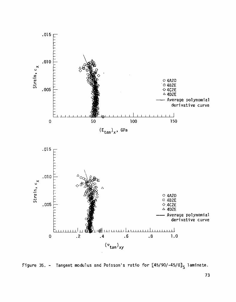
backward difference results. The plots of the [45/90/-45/0]3 laminate response
(fig. 35) show a more gradual stiffness loss and Poisson's ratio change, which
initiates at the 0.006 strain level. Although an initial edge replicate of one
specimen shows the presence of 90° ply cracks at zero stress, possibly due to
specimen machining, the earliest indication of additional splitting in 90° plies
11
occurs in an edge replicate taken at a strain of 0.0063. Delaminations do not
appear below a strain of 0.007 and do not grow extensively at higher strains. For
this laminate, the polynomial derivative curves agree with the finite difference
results. Both quasi-isotropic laminates exhibit splitting in the 90' plies, but
the laminate with the two adjacent 90" plies begins to split at a lower strain than
the one with isolated 90" plies, which are not at the surface.
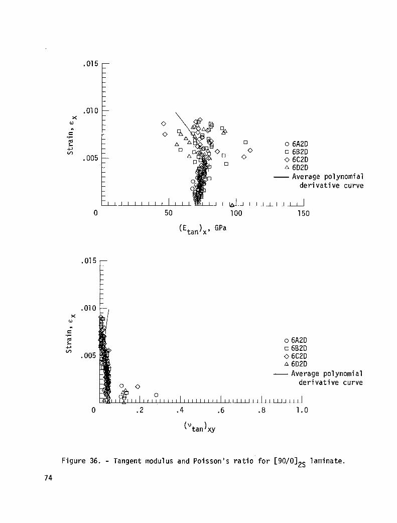
The plot of the tangent modulus for the [90/O]2S laminate (fig. 36) shows a
slight stiffness drop and a great deal of scatter starting at a strain of 0.004,
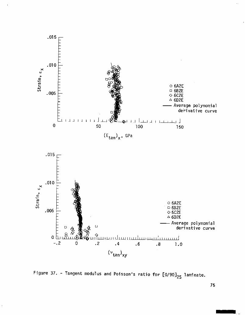
while the corresponding plot for the [0/9O],S laminate (fig. 37) exhibits nearly
the same stiffness loss, but displays comparatively little scatter. The 90" plies
of the [0/90]2S laminate, two of which are adjacent, appear to begin splitting at
the same strain as the 90" plies of the [90/0]2S laminate, each of which is
isolated from the others. Two of the 90" plies in the [90/0]2S laminate are at
the surface, however, and are each constrained by only one adjacent ply. The
relative proximity of the 90° plies to the surface mounted strain gages apparently
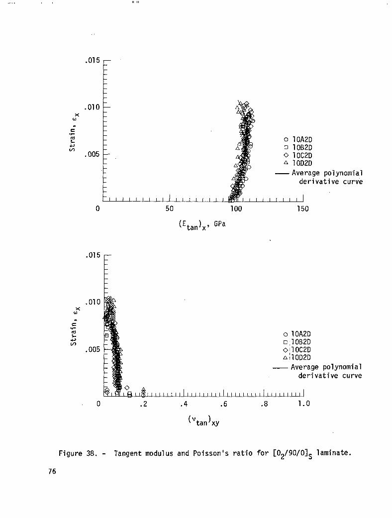
determines the relative magnitude of the scatter. Plots of the [0,/9O/O]S and
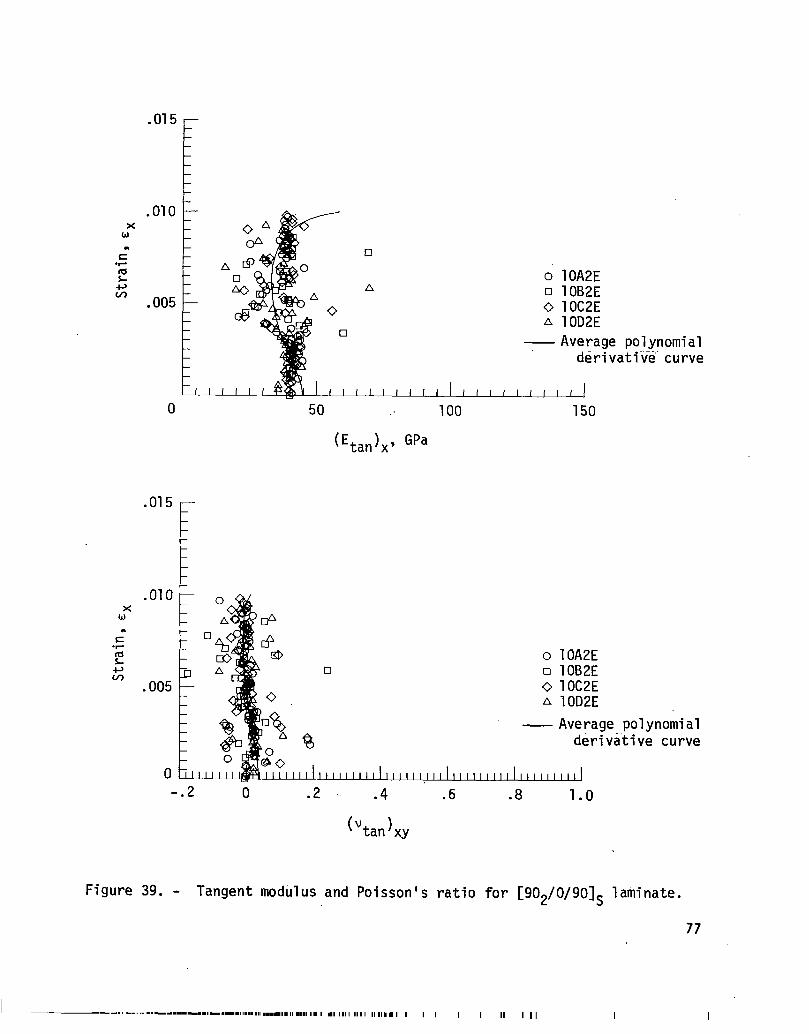
[902/O/90]S tangent moduli shown in figures 38 and 39 appear to support this.
The [902/O/90]S laminate, with two adjacent 90" plies at each surface, shows a
stiffness drop and considerable scatter at a strain of about 0.0035. The tangent
modulus plot in figure 39 indicates the inability of the polynomial to model
derivatives when the data is ill-behaved.
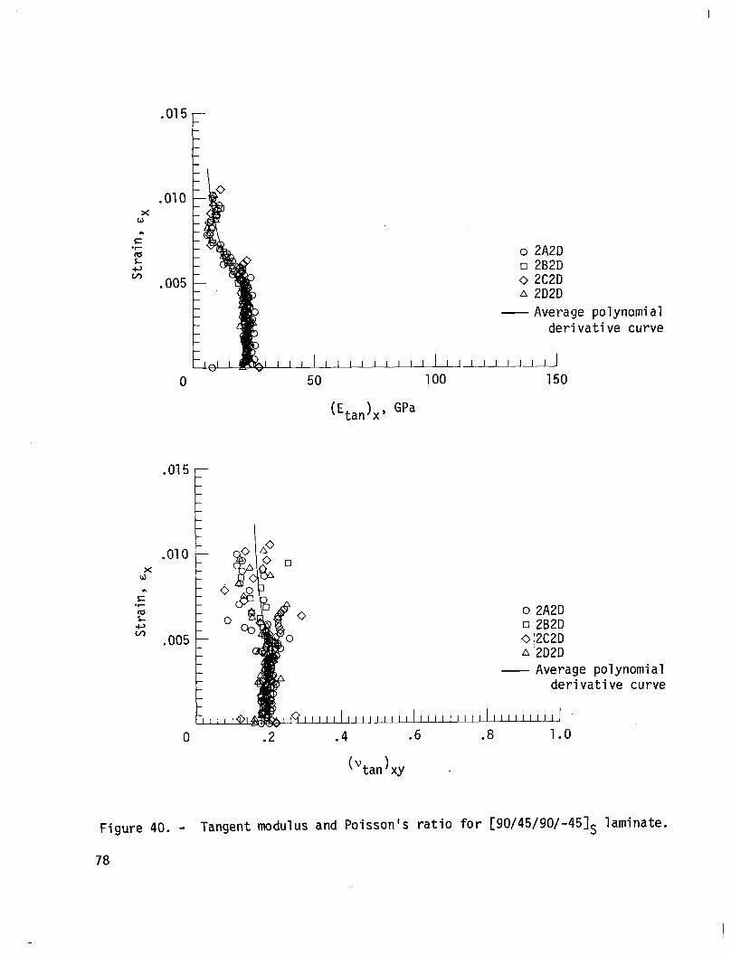
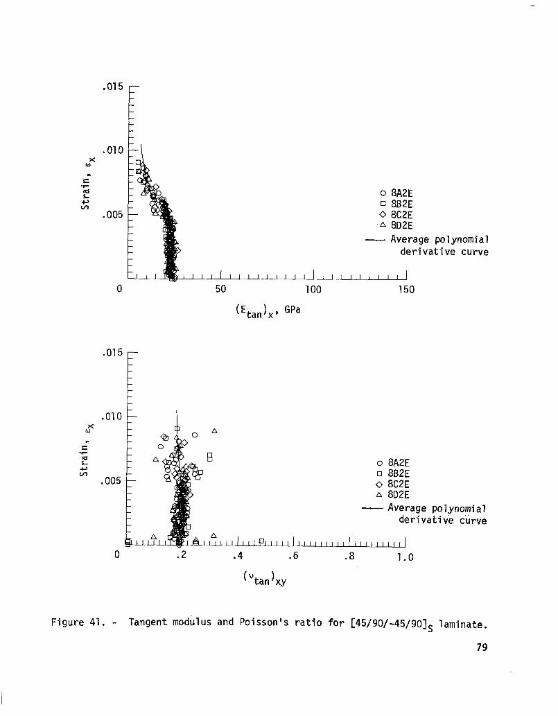
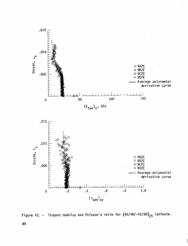
Stiffness and Poisson's ratio plots for the [90/45/90/-45]S,
[45/90/-45/9O]S, and [45/90/-45/9012S laminates shown in figures 40, 41, and 42
exhibit nearly identical behavior. The stiffness of each laminate drops at
approximately the same 0.005 level of strain while scatter increases in the
Poisson's ratio plots at that strain. Two of the laminates have two adjacent 90"
plies at the center while the other has isolated 90' plies at the surface.
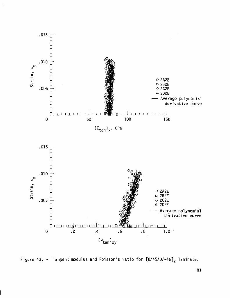
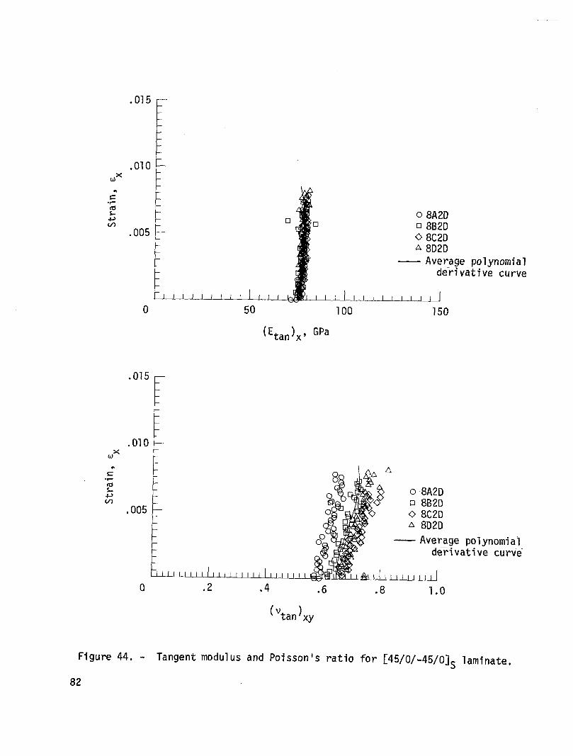
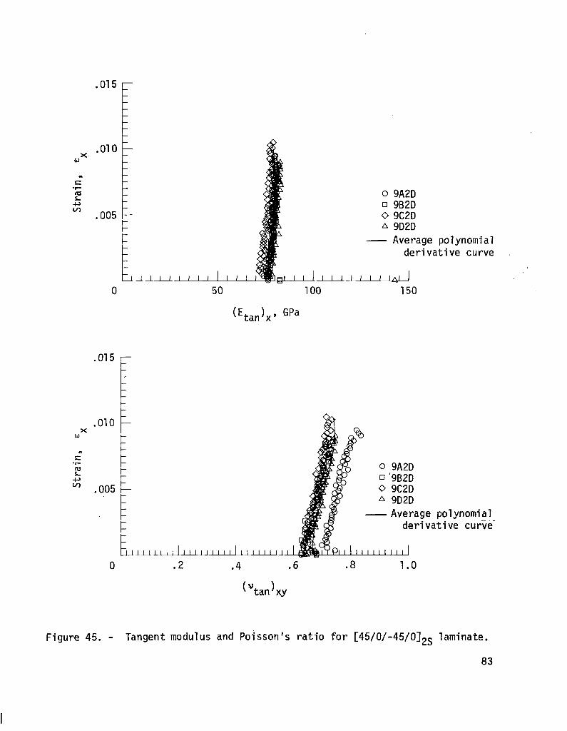
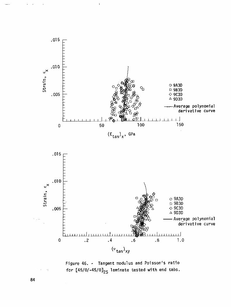
With the exception of the plots for the end-tabbed specimens, the tangent
modulus and Poisson's ratio plots for the [O/45/0/-45]S, [45/O/-45/O]S, and
[45/O/-45/O]2S laminates shown in figures 43, 44, 45, and 46 are similar. The
source of the scatter in the plots of figure 46 is not apparent.
12
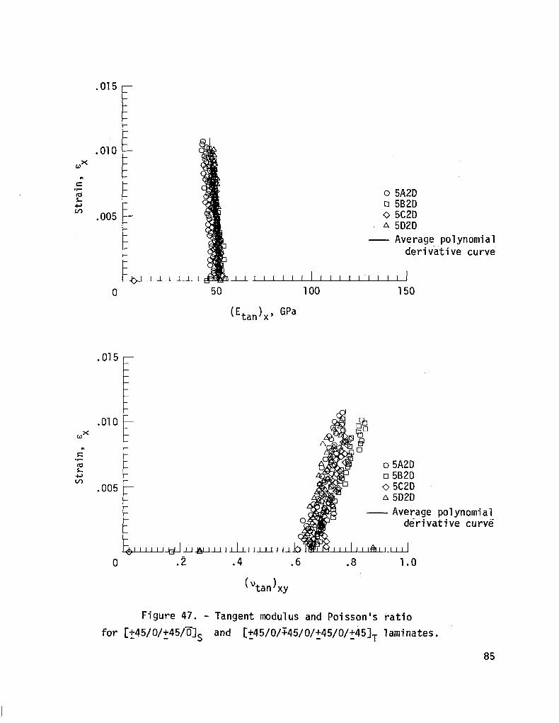
The error in the stacking sequence of laminate number five (see table I) had
no discernable effect on the moduli and Poisson's ratios plotted in figures 47 and
48. In each case the polynomial adequately modeled the material behavior by
smoothing scatter while retaining the essential character of the data. _
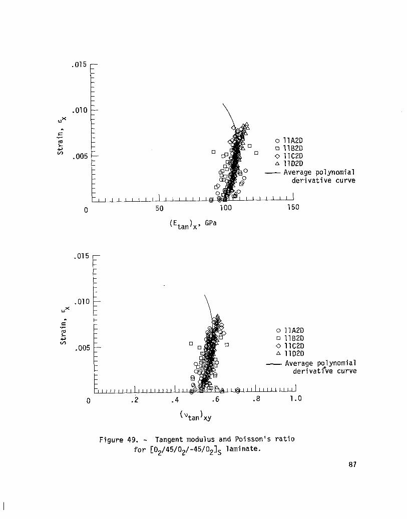
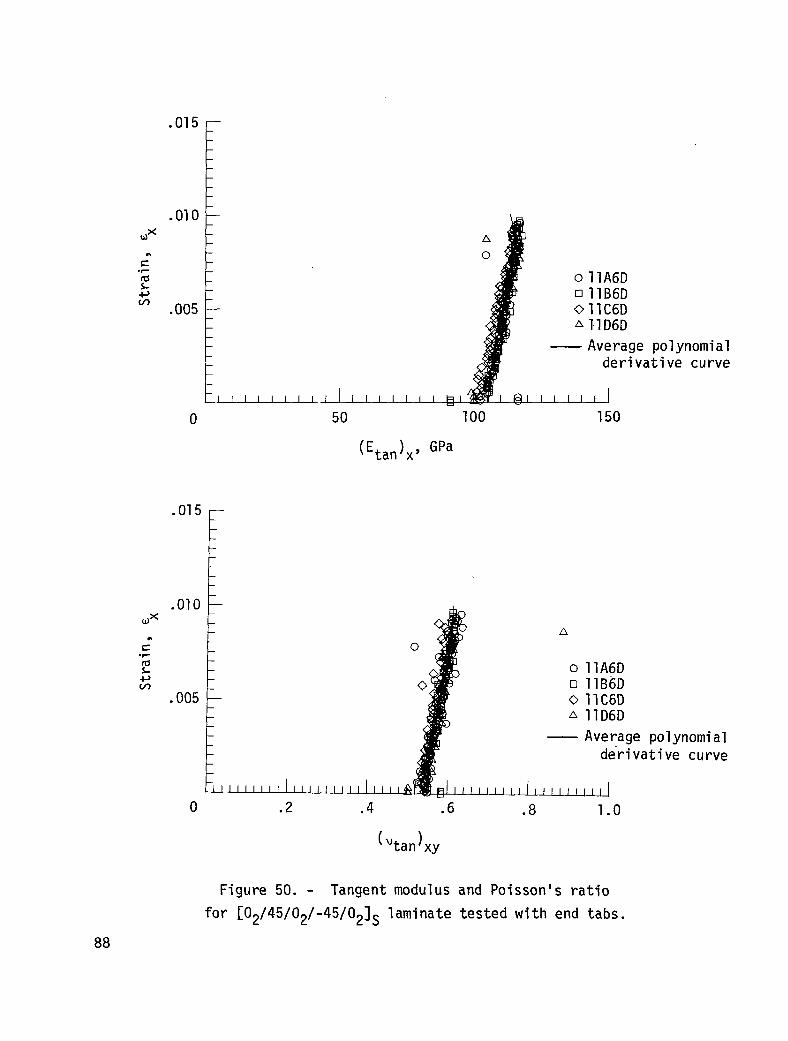
A comparison of figures 49 and 50 shows that end-tabs, in additi.on to
improving strength, reduce data scatter and enable the polynomial to accurately fit
the tangent modulus and POiSSOn's ratio for the [02/45/O,/-45/02]S laminate.
Since this laminate is composed primarily of O" plies, it is not surprising that
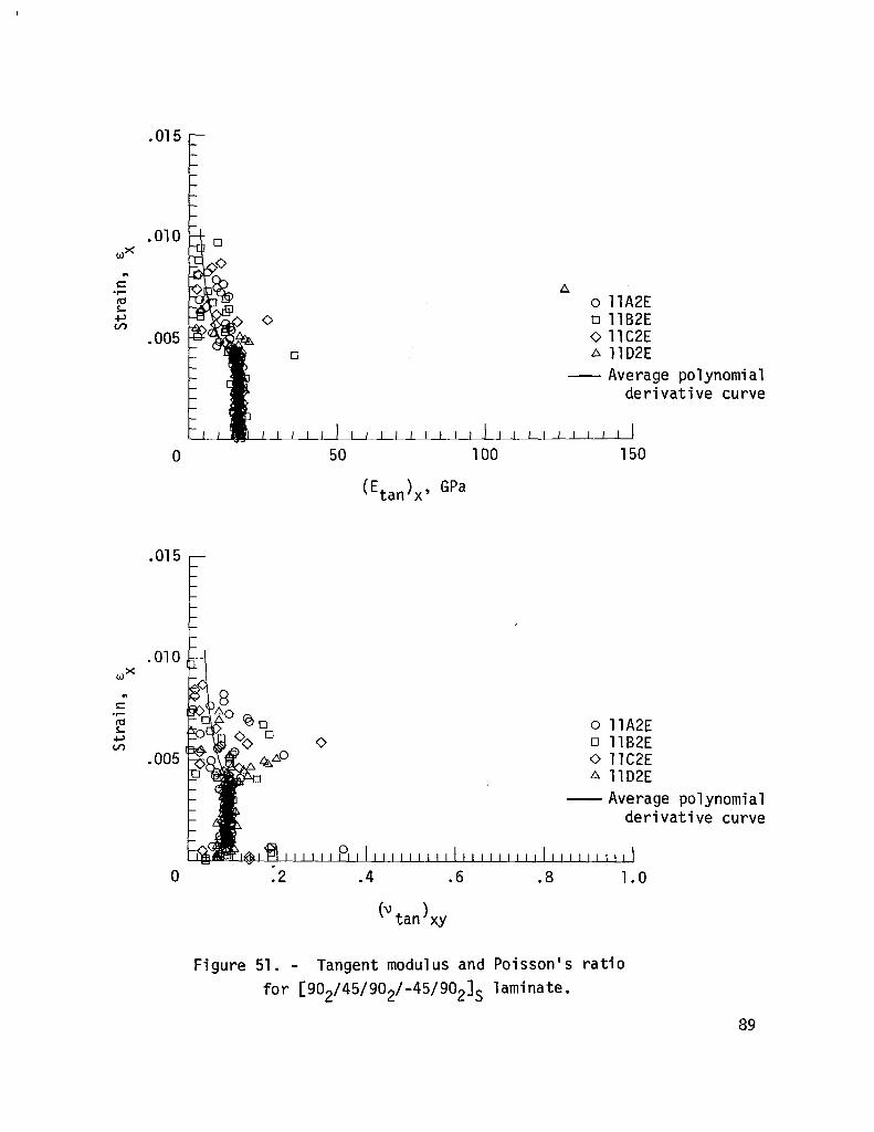
the stiffness increases with increasing strain as in the [O]a laminate. The plots
of the [90,/45/90,/-45/9O,]S stiffness and Poisson's ratio shown in figure 51
show linear behavior to a strain of about 0.0035 at which point the laminate
suffers a substantial stiffness loss. The 90° plies at the surface of the laminate
again contribute to data scatter.
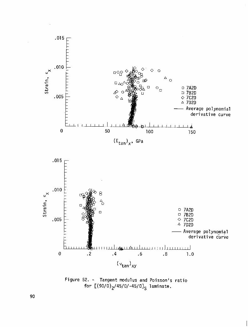
The [(90/O)2/45/O/-45/O]S laminate plots in figure 52 show.stiffness drop
and scatter at a strain of about 0.005 because of the 90" plies at the surface.
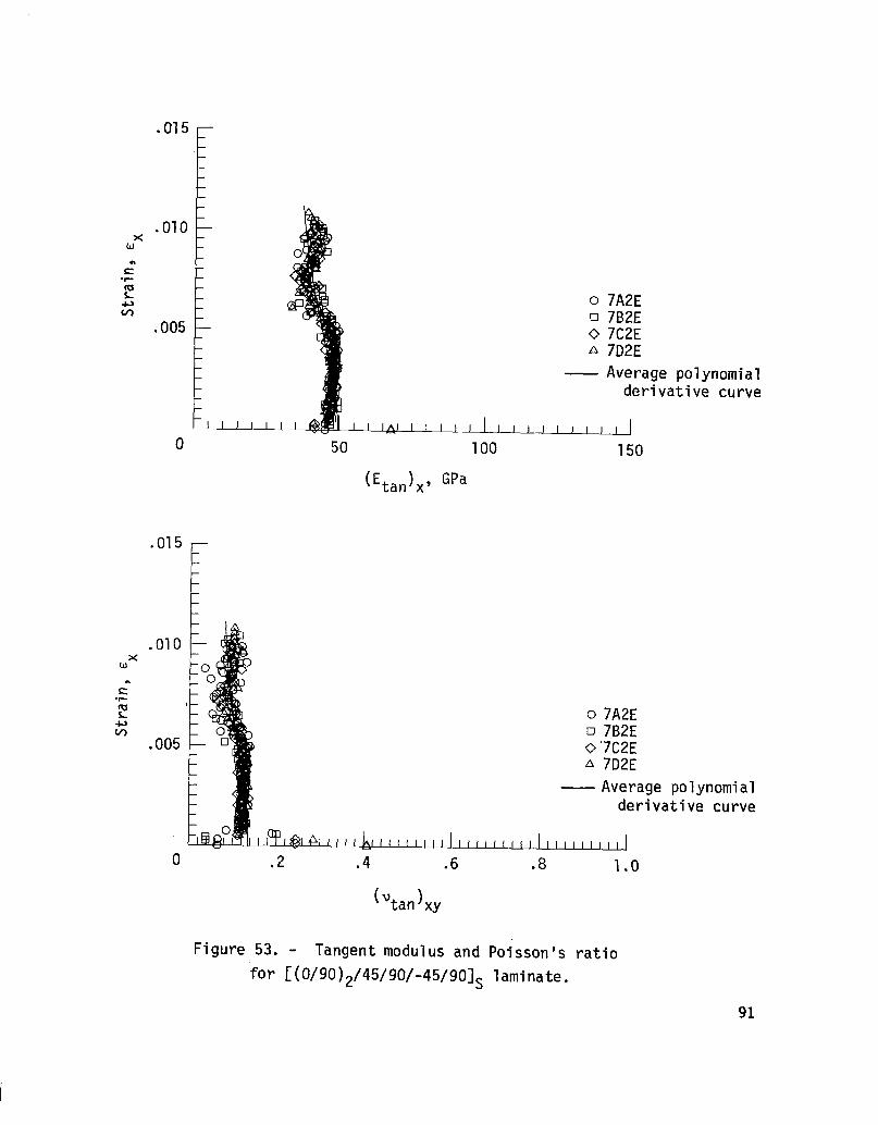
The [(O/90),/45/90/-45/9O]S laminate , with two adjacent 90° plies at the center,
also exhibits a stiffness drop at a strain of 0.005, as seen in figure 53, but
comparatively little scatter.
Experimental values of Young's modulus and Poisson's ratio for each laminate
were calculated using the linear terms of the least squares polynomials for each
specimen. These laminate elastic values and the average ultimate tensile strength
of each laminate are displayed in 'figures 54, 55, and 56 in the form of Cordell
(ref. 6) plots. Cordell plots are two-dimensional projections of three-dimensional
plots presented so as to enable the viewer to visualize the original 3-D form.
Data points in each figure are plotted as symbols. A fourth order polynomial
surface, plotted as solid lines, was determined for each figure by the method of
least squares to aid in visualizing the behavior of the laminate constants
presented. In some cases there are laminates which have different stacking
sequences but possess the same percentages of O" plies, 90' plies, and 245" plies.
In the plots of Young's modulus and Poisson's ratio, the differences between
experimental values in these cases are so slight as to be inconsequential and the
fourth order surfaces were calculated using all the data points. It is obvious
from figure 56, however, that two laminates with the same percentages of 0" plies,
13
90" plies, and +45" plies can have substantially different strengths. The surface
plotted in figure 56 was fit only to the greatest value corresponding to a given
ply composition. Although the plots in figures 54 and 56 appear to have the same
general shape, examination of table V will show that failure strains vary among the
different laminates.
Laminate Analysis
Classical laminate analysis was performed for each laminate in this study.
Values of Young's modulus and Poisson's ratio from the analysis appear in table V
with experimentally determined values. Although classical laminate analysis
predicts laminate constants to within a few percent of measured values in most
cases, there are several substantial deviations which must be explained. The
largest of these, the error in the [9O]s Poisson's ratio prediction, suggests that
the omission of transverse sensitivity corrections may have led to biases in
strain data which appear as incorrect experimental laminate constants. Although
the transverse sensitivity coefficient is unknown, a typical value of 1 percent is
sufficient to account for the Poisson's ratio errors for the [901s, [0,/90/0]9,
[90/45/90/-4513, [45/90/-45/9O]s, [45/90/-45/90]2s, and
[~45/90/745/90/~45/90/+451T 1 ami nates. The Poisson's ratio error for the
[902/45/902/-45/902]s laminate is only halved by a transverse sensitivity of 1
percent and other errors are relatively unaffected.
While the transverse sensitivity of the strain gages appears to be responsible
for at least part of the disagreement between experimental and laminate analysis
values of elastic constants, it is not sufficient to explain all of the errors.
Another possible source of error is the least squares curve fitting procedure from
which experimental laminate constants are determined. As mentioned earlier, there
appear to be cases in which the polynomials poorly model the slopes of the stress-
strain curves. The most obvious examples are the Poisson's ratio plot of the
[45/O/-45/9013 laminate in figure 34 and the tangent modulus plot of the
[902/O/90]s laminate in figure 39 for which the polynomial curves and finite
difference points clearly differ.
14
SUMMARY OF RESULTS
The tensile behavior of a variety of T300/5208 graphite/epoxy laminates was
examined. Stress-strain curves were plotted for each specimen for uniaxial
monotonic loading to failure. Fourth order polynomial curves were fit to the data
in order to get average stress-strain curves. Stiffness and Poisson's ratio,
obtained by differentiating the stress-strain polynomia.ls, were plotted against
longitudinal strain for each laminate. Experimentally determined values of Young's
modulus and Poisson's ratio were compared with classical laminate analysis results.
Except for a few laminates, classical laminate analysis and experiments gave
the same elastic constants. Predictions and measurements of Poisson's ratio
differed for only a few laminates with very low Poisson's ratios. A combination of
low transverse strain and the failure to account for the transverse sensitivity of
the foil strain gages appeared to be primarily responsible for the difference
rather than any inherent limitation of the laminate analysis. Measured and
predicted values of Young's modulus differed in cases where sharp changes in the
slope of the stress-strain curve limited the ability of the polynomial to model the
slope. Overall, the laminate analysis results were within the experimental
accuracy of the measurements.
Sharp changes in the slopes of stress-strain curves occurred only for
laminates containing 90° plies. Laminates with four adjacent 90' plies at the
center or two adjacent 90" plies at the surface exhibited stiffness drops at a
strain approximately equal to the ultimate tensile strain of the [9O]a laminate.
Those with two adjacent 90" plies at the center or isolated 90° plies at the
surface showed stiffness loss at strains between 0.004 and 0.005 while laminates
with isolated 90" plies not at the surface experienced stiffness loss at strains
between 0.006 and 0.007.
While the polynomial method did not adequately model the slopes of ill-behaved
stress-strain curves, it accurately modeled the slopes of the [Ola, [9O]s, and
[?45]2S stress-strain curves from which lamina elastic constants were deter-
mined. Because differences between laminate analysis predictions and experimental
data analysis results appear to be due to data analysis limitations, it is felt
that laminate elastic constants from the laminate analysis should be used when
initial moduli are required.
15
Because of the large variety of laminates, there appears to be no simple
failure model which can accurately predict tensile strength in every case. In
several cases, delamination growth or gripping difficulties caused laminates to
fail at. unexpectedly low strains. Because tapered end-tabs exert tensile stresses
normal to the specimen surfaces, their use improved gripping only for the
[02/45/02/-45/02]s laminate which has compressive interlaminar normal stresses
when tested in tension. In most instances failure strains fell in the range of 0.9
percent to 1.1 percent for both matrix and fiber dominated layups.
16
REFERENCES
1. Whitney, J. M.; and Kim, R. Y.: Effect of Stacking Sequence on the Notched
Strength of Laminated Composites. Composite Materials: Testing and Design (Fourth
Conference). ASTM STP 617, American Society for Testing and Materials, 1977, pp.
229-242.
2. Sova, 3. A.; and Poe, C. C., Jr.: Tensile Stress-Strain Behavior of
Boron/Aluminum Laminates. NASA TP-1117, 1978, p. 26.
3. Draper, N. R.; and Smith, H.: Applied Regression Analysis. Second ed. John
Wiley & Sons, Inc., 1981, pp. 91-92.
4. Jones, R. M.: Mechanics of Composite Materials. Scripta Book Company, 1975.
5. Rosen, B. W.: A Simple Procedure for Experimental Determination of the
Longitudinal Shear Modulus of Unidirectional Composites. Journal of Composite
Materials, Vol. 6, October 1972, pp. 552-554.
6. Cordell, T. M.: The Cordell Plot: A Way to Determine Composite Properties.
SAMPE Journal, Vol. 13, No. 6, Nov/Dec 1977, pp. 14-19.
7. Oplinger, D.: Studies of Tensile Specimens for Composite Material Testing.
Proceedings of the Technical Co-Operation Program (TTCP) Subgroup P - Materials
Technology, Technical Panel 3 - Organic Materials, Ottawa, Canada, May 1978.
8. Pagano, N. J.; and Pipes, R. B.: Some Observations on the Interlaminar
Strength of Compos ite Laminates. International Journal of Mechanical Sciences,
Vol. 15, 1973, pp. 679-688.
9. O'Brien, T. K.; Ryder, J. T.; and Crossman, F. W.: Stiffness, Strength,
Fatigue Life Relationships for Composite Laminates. Proceedings of the 7th Annual
Mechanics of Composites Review, Dayton, Ohio, October 1981, pp. 38-43.
17
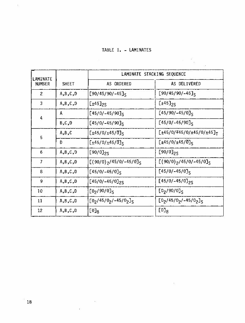
TABLE I. - LAMINATES
t- LAMINATE STACKING SEQUENCE 1 LAMINATE
NUMBER SHEET AS ORDERED
2 A,B,C,D [90/45/90/-451s
3 A,B,C,D [+4512s
A 4
[45/O/-45/9O]s
B,C,D [45/O/-45/9O]s
A,B ,C k45/0/+45/ulS 5
D c+45/0/+45mS
6 A,B,C,D L-WQS 7 A,B,C,D [(90/O) ,/45/%45/Ols
8 A,B,C,D c45/0/-45/01S
9 A,B,C,D [45/%45/01,s
10 A,B,C ,D [02/9w01s
11 A,B,C,D [O~/~~/~~/-~~/~~~s
12 A,B,C,D [o&j
AS DELIVERED
[90/45/90/-451s
[45/90/-45101s
[45/O/-45/9O]s
m[+45/o/+45/8]s I
L-WOI,,
c (90/O) 2/4wv-45/01s I
18
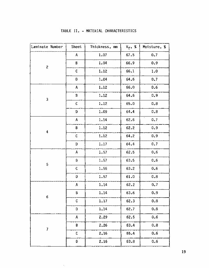
TABLE II. - MATERIAL CHARACTERISTICS
-aminate Number
2
3
4
5
6
7
- Sheet Thickness, mn Vf, % Moisture, %
A 1.07 67.5 0.7
B 1.04 66.9 0.9
C 1.12 66.1 1.0
D 1.04 64.6 0.7
C I 1.55 1 63.2 1 0.6 I I I
D I 1.57 1 61.0 1 0.8
A 1 1.14 1 62.2 1 0.7
B I
1.14 1 63.6 1 0.9
c I 1.17 \ 62.3 \ 0.8 1
D 1 1 62.7 1 0.8
D 1 2.16 1 63.8 1 0.6
19
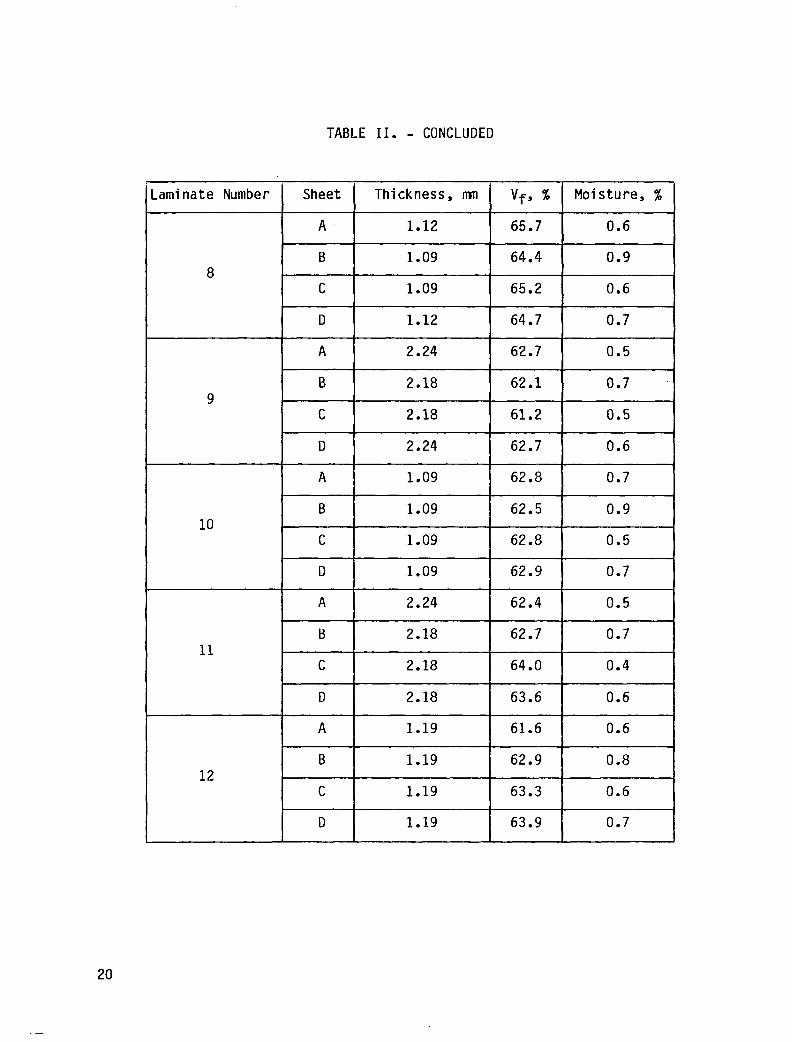
TABLE II. - CONCLUDED
8
A 2.24 62.4 0.5
B 2.18 62.7 0.7 11
C 2.18 64.0 0.4
D 2.18 63.6 0.6
A 1.19 61.6 0.6
B 1.19 62.9 0.8 12
C 1.19 63.3 0.6
D 1.19 63.9 0.7
Laminate Number
20
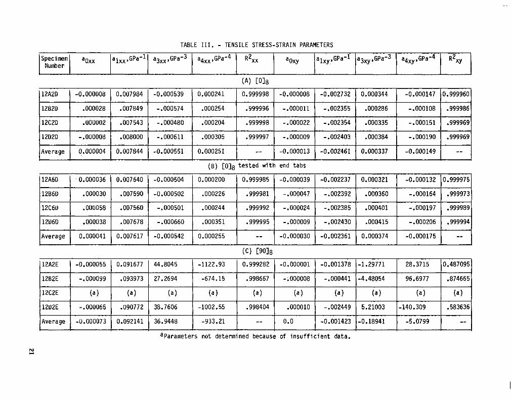
TABLE III. - TENSILE STRESS-STRAIN PARAMETERS
Specimen aoxx alxx,GPaml Number
a3xx,GPa-3 a4xx,GPa-4 R2xx aoxy alxy,GPa-1 a3xy,GPa-3 a4xy,GPa-4 R2xy
(A) co18 12A20 -0.000008 0.007984 -0.000539 0.000241 0.999998 -0.000008 -0.002732 0.000344 -0.000147 0.999960
128213 .000028 .007849 -.000574 .000254 .999996 -.000011 -.002355 .000286 -.000108 .999986
12C20 .000002 .007543 -.000480 .000204 .999998 -.000022 -.002354 .000335 -.000151 .999969
12D20 -.000008 .008000 -.000611 .000305 .999997 - .000009 -.002403 .000384 -.000190 .999969
Average 0 ,. 000004 0.007844 -0.000551 0.000251 -- -0.000013 -0.002461 0.000337 -0.000149 --
(B) [0]8 tested with end tabs
I 12A60 1 0.000036 1 0.007640 1 -0.000504 1 0.000200 1 0.999985 1 -0.000039 ( -0.002237
I 12B60 I .000030 1 .007590 1 -0.000502 ) .000226 ) .999981 1 -.000047 1 -.002392 .000360 1 -.000164 1 .9999731
I 12C6U I .000058 1 .007560 1 -.000501 1 .000244 ) .999992 1 -.000024 1 -.002385
I 12ll6D I .000038 I .007678 I -.000660 I .000351 I .999995 I -.000009 I -.002430
I Average I
0.000041 1 0.007617 1 -0.000542 1 0.000255 1 -- 1 -0.000030 1 -0.002361
(c) [go18 12A2E -0.000055 0.091677 44.8045 -1122.93 0.999282 -0.000001 -0.001378
12B2E -.oouo99 .093973 27.2694 -674.15 .998667 -;000008 -.000441
12C2E (4 (4 (a) (4 (4 (4 (a)
12U2E -.000065 .090772 38.7606 -1002.55 .998404 .000010 -.002449
Average -0.000073 0.092141 36.9448 -933.21 -- 0.0 -0.001423
0.000321 ) -0.000132 lo.9999751
.000401 1 -.000197 1 .999989)
.000415 I -.000206 I .999994 I 0.000374 I -0.000175 -- l I
-1.29771 28.3715 I 0.487095
-4.48054 1 96.6977 1 .874665!
(4 I (a) I (a) I 5.21003 I -140.309 I .583636 I
-0.18941 I -5.0799 I -- I aparameters not determined because of insufficient data.
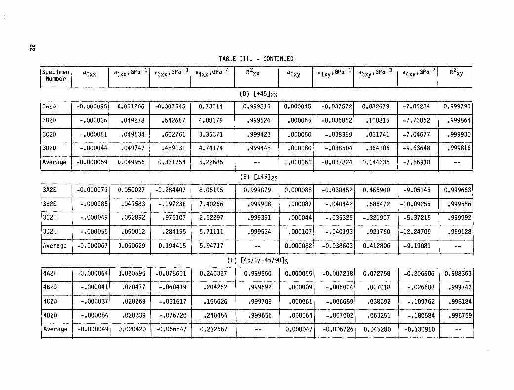
TABLE III. - CONTINUED
Specimen Number
aoxx alxx,GPa-1 a3xx,GPa-3 a4xx,GPa-4 R2xx aoxy a1xys GPa-l a3xy, GPa-3 a4xy,GPa-4 R2xy
(D) [+45h
3A2U -0.uuuo95 0.051266 -0.307545 8.73014 0.999815 0.000045 -0.037572 0.082679 -7.06284 0.999795
3B2U -.UUUO36 .049278 .542667 4.08179 .999526 .000065 -0.036852 .108815 -7.73062 .999864
3C2U -.OOUU61 .049534 .602761 3.35371 .999423 .000050 -.038369 .031741 -7.04677 .999930
3u2u -.ouuu44 .049747 .489131 4.74174 .999448 .000080 -.038504 .354106 -9.63648 .999816
Average -0. uuuo59 0.049956 0.331754 5.22685 -- 0.000060 -0.037824 0.144335 -7.86918 --
3A2E -0.000079 0.050027 -0.284407 8.05195 0.999879 0.000088 -0.038452 0.465900 -9.05145 0.999663
3B2E -.000085 .049583 -. 197236 7.40266 .999908 .000087 -.040442 .585472 -10.09255 .999586
3C2E -.000049 .052892 .975107 2.62297 .999391 .000044 -.035326 -.321907 -5.37215 .999992
3U2E -.000055 .050012 .284195 5.71111 .999534 '.000107 -.040193 .921760 -12.24709 .999128
Average -0.000067 0.050629 0.194415 5.94717 -- 0.000082 -0.038603 0.412806 -9.19081 --
(F) CWW-4WOls 4A2E -0.000064 0.020595 -0.078631 0.240327 0.999560 0.000055 -0.007238 0.072758 -0.206606 0.988363
4B2U -.000041 .020477 - .060419 .204262 .999692 .000009 -.006004 .007018 -.026688 .999743
4C20 -.000037 .020269 -.051617 .165626 .999709 .000061 - .006659 .038092 -.109762 .998184
4020 -.000054 .020339 -.076720 .240454 .999656 .000064 -.007002 .063251 -..180584 .995769
Average -0. ouoo49 0.020420 -0.066847 0.212667 mm 0.000047 -0.006726 0.045280 -0.130910 --
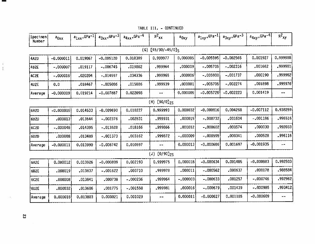
TABLE III. - CONTINUED
Specimen aoxx alxx,GPa-1 a3xx,GPa-3 a4xx,GPa-4 R2xx aoxy alxy,GPa-l a3xy,GPa-3 a4xy,GPa-4 R2xy Number
(G) l?WW-WOls
4A2D -0.000011 0.019067 -0.005120 0.018309 0.999977 0.000005 -0.005595 -0.002565 0.001927 0.999988
4B2E -.000007 .019117 -.006745 .019862 .999964 .000009 -.005705 -.002316 .001662 .999981
4C2E -.OUUO18 .020204 -.014597 .034336 .999965 .000006 -.005900 -.001737 .000190 .999982
4U2E 0.0 .018467 -.005086 .015886 .999939 .000001 -.005705 -.002274 .001898 .999976
Average -0.000009 0.019214 -0.007887 0.022098 -- 0.000005 -0.005726 -0.002223 0.001419 -- +
(HI CWOl2s
6A2D ‘-U.000016 0.014533 -0.009690 0.018227 0.999993 0.000032 -0.000816 0.004268 -0.007112 0.938259
6B2U .000013 .013544 -.002376 .002831 .999931 .000015 -.000732 .001604 -.001186 .996516
6C2D -.000048 .014395 -.013528 .018166 .999866 .000012 -.000602 .000574 .000030 .992033
6D2D .000008 .013489 -.001373 .003162 .999872 -.000009 -.000595 .000341 .000528 .996116
Average -0.000011 0.013990 -0.006742 0.010597 -- 0.000013 -0.000686 0.001697 -0.001935 --
(J) CWOlx 6A2E 0.000012 0.013926 -0.000809 0.002193 0.999975 0.000018 -0.000634 0.001405 -0.000883 0.992503
6B2E .uooo19 .013837 -.001622 .003710 .999978 .000011 -.000562 .000637 .000178 .988584
6C2E .000008 .013841 .000738 -.000236 .999964 -.000003 .-.000633 .001257 -.000746 .992!i62
6D2E .000032 .013606 .001775 -.001550 .999981 .000016 -.000679 .001439 - .000985 .993412
Average 0.000018 0.013803 0.000021 0.001029 -- 0.000011 -0.000627 0.001185 -0.000609 --
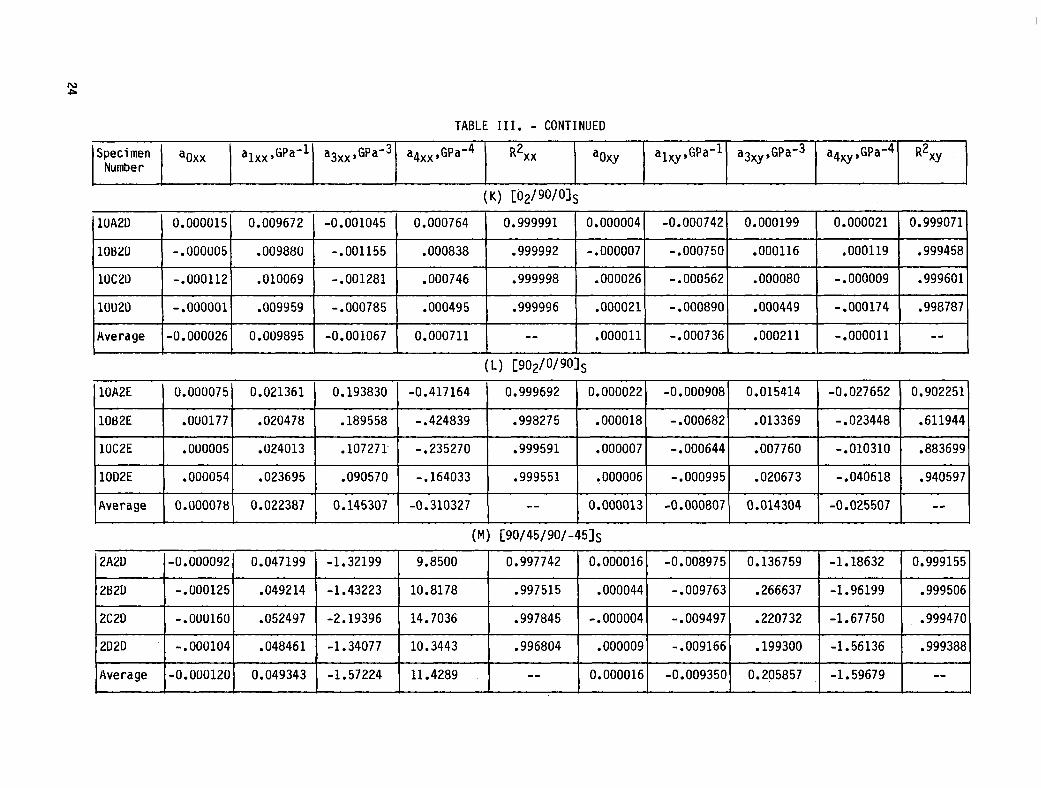
TABLE III. - CONTINUED
Specimen Number
aoxx alxx,GPawl a3xx,GPa-3 a4xx,GPa-4 R2xx aoxy alxy,GPaml a3xy,GPa'3 a4xy,GPa-4 R2xy
(lUA2D 1 0.0000151 0.009672 1 -0.001045 1 0.000764
llOB2U 1 -.0000051 .009880 [ -.001155 1 .000838
llOC2D 1 -.U001121 .010069 1 -.00128l 1 .000746
(lOU2D 1 -.OOOOOll .009959 1 -.000785 1 .000495
I Average I -0.000026 I 0.009895 I -0.001067 I 0.000711
K) [02/90/O]
0.999991
.999992
.999998
.999996
--
,
0.000004 -0.000742 0.000199 0.000021 0.999071
-.000007 -.000750 .000116 .000119 .999458
.000026 -.000562 .000080 -.000009 .999601
.000021 - .000890 .000449 -.000174 .998787
.000011 -.000736 .000211 -.000011 --
(L) [902/0/9OlS
lUA2E u.oouo75 0.021361 0.193830 -0.417164 0.999692 0.000022 -0.000908 0.015414 -0.027652 0.902251
1082E .uuo177 .020478 .189558 -.424839 .998275 .000018 -.000682 .013369 -.023448 .611944
lOC2E .uuuoo5 .024013 .107271' -.235270 .999591 .000007 -.000644 .007760 -.010310 .883699
lOD2E .000054 .023695 .090570 -.I64033 .999551 .000006 -.000995 .020673 -.040618 .940597
Average 0.000078 0.022387 0.145307 -0.310327 -- 0.000013 -0.000807 0.014304 -0.025507 --
(M) [90/45/90/-451s
2A2U -0.000092 0.047199 -1.32199 9.8500 0.997742 0.000016 -0.008975 0.136759 -1.18632 0.999155
2B2D -.000125 .049214 -1.43223 10.8178 .997515 .000044 - .009763 .266637 -1.96199 .999506
1 2C2D 1 -.OUU160( .052497 1 -2.19396 1 14.7036 1 .997845 1 -.0000041 -.0094971 .220732 1 -1.67750 1 .999470(
]2D2D 1 -.oou104~ .048461 1 -1.34077 1 10.3443 1 .996804 1 .0000091 -.009166) .I99300 1 -1.56136 1 .9993881
IAverage I-O.UUO1201 0.049343 I -1.57224 I 11.4289 ] -- I 0.0000161 -0.0093501 0.205857 1 -1.59679 1 -- 1
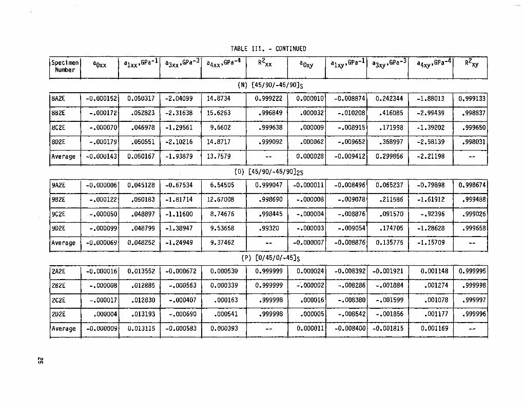
TABLE III. - CONTINUED
Specimen aoxx Number
alxx,GPa-l a3xx,GPa-3 a4xx,GPa-4 R2xx aoxy alxy,GPa-l a3xy,GPa-3 a4xy,GPa-4 R2xy
c (N) [45/90/-45/9O]s
8A2E -0.000152 0.050317 -2.04099 14.8734 0.999222 0.000010 -0.008874 0.242344 -1.88013 0.999133
8B2E -.000172 .052823 -2.31638 15.6263 .996849 .000032 -.010208 .416085 -2.99439 .998837
8C2E -.000070 .046978 -1.29561 9.6602 .999638 .000009 -.008915 .171998 -1.39202 .999650
802E -.000179 .050551 -2.10216 14.8717 .999092 .000062 -.009652 .368997 -2.58139 .998031
Average -0.000143 0.050167 -1.93879 13.7579 -- 0.000028 -0.009412 0.299856 -2.21198 --
(0) c45/90/-w9012s 9A2E -U.UOUOO6 0.045128 -0.67534 6.54505 0.999047
9B2E -.000122 .050183 -1.81714 12.67008 .998690
9C2E -.000050 .048897 -1.11600 8.74676 .998445
9D2E -.000099 .048799 -1.38947 9.53658 .99320
Average -U.U00069 0.048252 -1.24949 9.37462 --
-0.000011 -0.008496 0.065237 -0.79898 0.998674
-.000008 -.009078 .211586 -1.61912 .999488
-.000004 -.008876 .091570 - .92396 .999026
-.000003 -.009054 .I74705 -1.28628 .999658
-0.000007 -0.008876 0.135775 -1.15709 --
(PI [O/45/0/-451s
2A2E -0.000016 0.013552 -0.000672 0.000530 0.999999 0.000024 -0.008392 -0.001921 0.001148 0.999995
2B2E -.000008 .012885 -.000563 0.000339 0.999999 -;000002 -.008286 -.001884 .001274 .999998
2C2E -.ouoo17 .012830 -.000407 .000163 .999998 .000016 -.008380 -.001599 .001078 .999997
2D2E .oouoo4 .013193 -.000690 .000541 .999998 .000005 -.008542 -.001856 .001177 .999996
Average -0.000009 u.013115 -0.000583 0.000393 -- 0.000011 -0.008400 -0.001815 0.001169 --
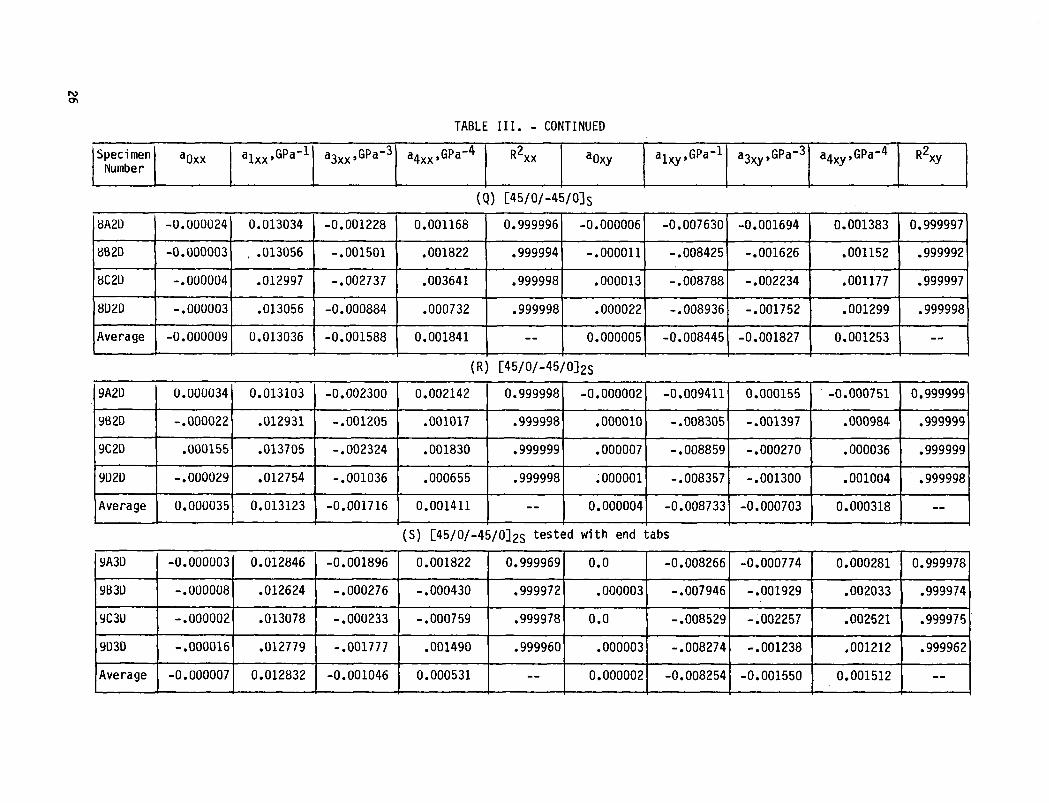
TABLE III. - CONTINUED
Specimen aoxx alxx ,GPa-l a3xx,GPa-3 a4xx,GPa-4 R2xx Number
aoxy alxy,GPa-l a3xy,GPa-3 a4xy,GPa-4 R2xy
(Q) [45/O/-45101s
8A2D -U.OUUU24 0.013034 -0.001228 0.001168 0.999996 -0.000006 -0.007630 -0.001694 0.001383 0.999997
8820 -0.000003 , .U13056 -.001501 .001822 .999994 -.000011 -.008425 -.001626 .001152 .999992
8C2U -.000004 .012997 -.002737 .003641 .999998 .000013 -.008788 -.002234 .001177 .999997
8U2D -.uuuoo3 .013056 -0.000884 .000732 .999998 .000022 -.008936 -.001752 .001299 .999998
Average -0.000009 0.013036 -0.001588 0.001841 -- 0.000005 -0.008445 -0.001827 0.001253 --
9A2D U.UUUU34 0.013103 -0.002300 0.002142 0.999998 -0.000002 -0.009411 0.000155 -0.000751 0.999999
YB2D -.000022 .012931 -.001205 .001017 .999998 .000010 -.008305 -.001397 .000984 .999999
YCPD .uoo155 .013705 -.002324 .001830 .999999 .000007 -.008859 -.000270 .000036 .999999
YD2U -.oouo29 .012754 -.001036 .000655 .999998 ; 000001 -.008357 -.001300 .001004 .999998
Average U.000035 0.013123 -0.001716 0.001411 -- 0.000004 -0.008733 -0.000703 0.000318 --
' (S) [45/O/-45/0]2S tested with end tabs
YA3D -0.000003 0.012846 -0.001896 0.001822 0.999969 0.0 -0.008266 -0.000774 0.000281 0.999978
9830 -.000008 .012624 -.000276 -.000430 .999972 .000003 - .007946 - .001929 .002033 .999974
YC3U -.000002 .013078 -.000233 -.000759 .999978 0.0 - .008529 -.002257 .002521 .999975
9D3D -.000016 .012779 -.001777 .001490 .999960 .000003 -.008274 -.001238 .001212 .999962
Average -0.000007 0.012832 -0.001046 0.000531 -- 0.000002 -0.008254 -0.001550 0.001512 --
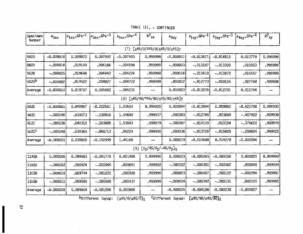
TABLE III. - CONTINUED
Specimen Number
aOxx alxx,GPa-1 a3xx,GPa-3 a4xx,GPa-4 R2xx aoxy alxy,GPa-1 a3xy,GPa-3 a4xy,GPa-4 R2xy 7
(T) [+45/0/~45/0/&45/0/&45]T
5A2U -0.000018 0.020870 0.007992 -0.007403 0.999998 -0.000011 -0.013571 -0.0’14515 0.013779 0.999998
5820 -.000014 .019149 .006166 -.004594 .999999 -.000003 -.013187 -.013300 .010053 .999996
5C2D -.ooouu5 .019648 .004942 -.004224 .999998 .000014 -.013410 -.013872 .015457 .999998
5D2Db -.000002 .019522 .004827 -.004702 .999999 .OOOOl2 -.012773 -.009116 .007768 .999988
Average -0.000010 0.019797 0.005982 -.005231 -- 0.000003 -0.013235 -0.012701 0.011764 --
(u) [+45/90/r45/90/+45/90/~45]T
5A2E -U.UUUUtll 0.040467 -0.222561 1.83689 0.999928 0.000044 -0.013994 0.059080 -0.623788 0.999930
5B2E -.000046 .039073 -.138916 1.54680 .999937 .000003 -.012765 .003680 -.407922 .999930
5C2E -.000036 .040315 -.183805 1.53043 .999979 -.000007 -.014119 .010184 -.375622 .999970
5U2EC -.000040 .039365 -.066713 .85229 .999990 .000036 -.013715 -.015828 -.200684 .999922
Average -0.000051 0.039805 -0.152999 1.44160 -- 0.000019 -0.013648 0.014279 -0.402004 --
(V).jD2/45/02/-45/02IS
llA2U 0.000006 0.009963 -0.001778 0.001488 0.999990 0.000003 -0.005265 -0.000050 0.000020 0.999999
lltJ2U -.000002 .009924 -.000965 .000691 .999982 -;000022 -.005381 -.000062 .000048 .999999
llC2D -.OUUU16 .009744 -.001221 .000926 .999996 .000003 -.005407 .000122 -.000294 .999981
llU2U -.000011 .009585 -.000868 .000437 .999998 -.000004 - .005392 -.000131 .000120 .999995
Average -0.000006 0.009804 -0.001208 0.000886 -- -0.000005 -0.004186 -0.000030 -0.000027 --
bDifferent layup: [&45/0/&45/mS CDifferent layup: Clt45/90/f45/mS
Y
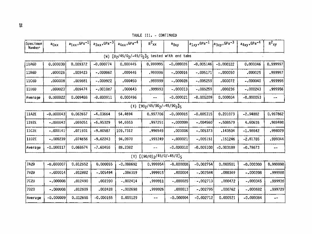
TABLE III. - CONTINUED
Specimen Number
aoxx alxx,GPa-l a3xx,GPa-3 a4xx,GPa-4 R2xx aoxy alxy,GPa-l a3xy,GPa-3 a4xy,GPa-4 R2xy
(W) [02/45/02/-45/02]S tested with end tabs
llA6D 0.000030 0.009372 -0.000774 0.000445 0.999995 -0.000026 -0.005146 -0.000122 0.000046 0.999997
llB6D .UOOO26 .009423 -.000862 .000445 .999996 -.000016 -.005171 -.000050 .000025 .999997
llC6D .000008 .009681 - .000922 .000450 .999999 -.000028 -.005259 .000072 -.000040 .999998
llU6D .OOUU23 .009474 -.001087 .000643 .999993 -.ooooi3 -.005259 .000236 -.000243 .999956
Average 0.000022 0.009488 -0.000911 0.000496 -- -0.000021 -0.005209 0.000034 -0.000053 --
llA2E -0.000043 0.062657 -4.03664 54.4694 0.997706 -0.000015 -0.005315 0.201073 -2.94882 0.997862
llB2E -.UUUU43 .065051 -6.95329 94.6553 .997251 - .000009 -.004560 - .508579 4.60618 .989498
llC2E -.000141 .071931 -9.80587 109.7312 .996549 .000006 -.005373 .I43504 -1.98642 .998029
llU2E -.000239 .074656 -9.62243 94.0970 .991249 -.000021 -.005151 .151246 -2.81785 .9993,44
Average -0.000117 0.068574 -7.60456 88.2382 -- -0.000010 -0.005100 -0.003189 -0.78673 --
(Y) [(90/0)2/45/O/-45/01,
7A2D -U.ODOOO7 0.012652 0.000055 -0.000692 0.999954 -0.000008 -0.002754 0.000501 -0.000300 0.999898
7B2U -.oouo14 .012882 -.005494 .006319 .999915 .000004 -.002584 .000349 -.000208 .999988
7C2U -.000008 .012490 .002390 -.002414 .999911 -.000025 .-.002713 .000472 -.000345 .999936
7D2D -.OOUUO8 .012609 .002428 -.002698 .999926 .000013 -.002795 .000762 -.000682 .999729
Average -0.000009 0.012658 -0.000155 0.000129 -- -0.000004 -0.002712 0.000521 -0.000384 --
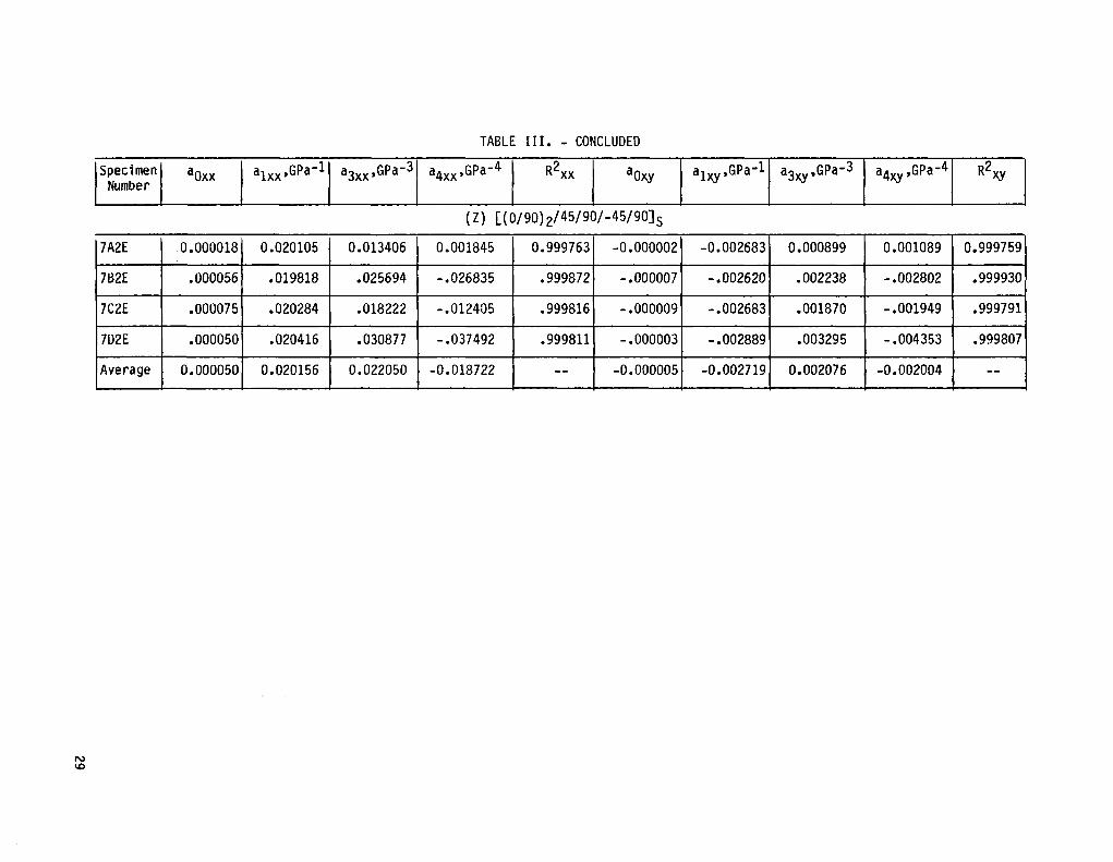
TABLE III. - CONCLUDED
Specimen aOxx alxx,GPa-1 a3xx,GPa-3 a4xx,GPa-4 R2xx Number
aoxy alxy,GPa-1 a3Xy,GPa-3 a4xy,GPa-4 R2xy
(Z) [(0/90)~/45/9~/-~~/9~1~
7A2E 0.000018 0.020105 0.013406 0.001845 0.999763 -0.000002 -0.002683 0.000899 0.001089 0.999759
7B2E .000056 .019818 .025694 -.026835 .999872 -.000007 -.002620 .002238 -.002802 .999930
7C2E .000075 .020284 .018222 -.012405 .999816 - .000009 -.002683 .001870 - .001949 .999791
7D2E .000050 .020416 .030877 - .037492 .999811 -.000003 - .002889 .003295 -.004353 .999807
Average I 0.0000501 0.020156 I 0.022050 I -0.018722 I -- I -0.000005~ -0.002719, 0.002076 I -0.002004 I -- I
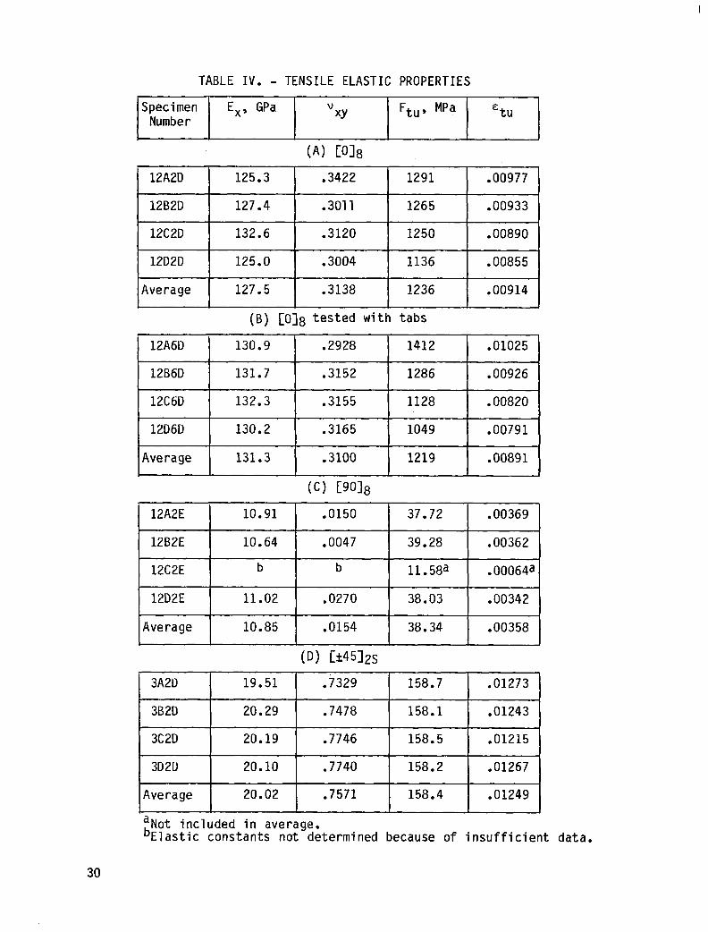
TABLE IV. - TENSILE ELASTIC PROPERTIES
Specimen E,, GPa Number
vxY Ftu, MPa %U
(A) CO18
12AZD I 125.3 I .3422 I
1291 I .00977 I 12B2D I 127.4 I .3011
I 1265 1 .00933 1
12C2D I
132.6 I
.3120 I
1250 1 .0089d 1 I
12D2D 125.0 .3004 1136 .00855
Average 127.5 .3138 1236 .00914
(B) [0]8 tested with tabs
I 12D6D I 130.2 I .3165 I 1049 I .00791 I
I Average I
131.3 I
.3100 I
(c) [go18
I 12A2E I 10.91 I .0150 I 37.72 I .00369 1 I 12B2E I 10.64 1 .0047 I 39.28 I -.00362 1
12C2E b b 11.58a .00064a
I 12D2E I 11.02 I .0270 I 38.03 1 .00342 1
I Average I 10.85 I .0154 I 38.34 I .00358 I (D) ih451zs
1 3A2D 1 19.51 I .7329 1 158.7 1 .01273 1
I 3B2D 1 20.29 1 .7478 1 158.1 -1 ~~ ~~~ .0124fl
3C2D 20.19 .7746 158.5 .01215
3D2D 20.10 .7740 158.2 .01267
Average 20.02 .7571 158.4 .01249
aNot included in average. bElastic constants not determined because of insufficient data.
30
_.--
TABLE IV. - CONTINUED
Specimen E x, GPa vxY Ftu, MPa "tu Number
ii). [-+4512s
I 3A2E 19.99 .7686 167.0 .01329
3B2E 20.17 .8157 171.4 .01379
-3CZE 18.91 .6679 139.9 ’ .01092
20.00 -~ 3D2E .8037 163.9 .01352
Average 19.75 .7625 160.6 .01288
(F > CW%W901s I 4A2E .3514 421.8 .00928 ~~
4BZD.-
I -...
48.56 --..I-
48~.84 ~~
.2932 344.6 .00733
4C2D 49.34 .3285 373.7 .00799
4D2D 49.17 .3443 443.6 .00955
Average 48.97 .3294 395.9 .00854
(‘4 CW9%WOls I 4A2D 52.45 .2934 506.0 .01004
?BZE 52.31 .2984 503.7 .00998
4C2E 49.50 .2920 482.1 .00972
4D2E 54.15 .3089 546.4 .01044 ..- --.-~- .~ Average 52.05 .2980 509.6 .01004
6A2D I 68.81 .0561 292.4a .00405a
6B2D 73.83 .0540 682.7 .00902
6C2D 69.47 .0418 683.5 .00923
--6D2D 74.14 .0441 633.6 .00864
Average 71.48 .0490 666.6 .00897
aNot included in average.
31
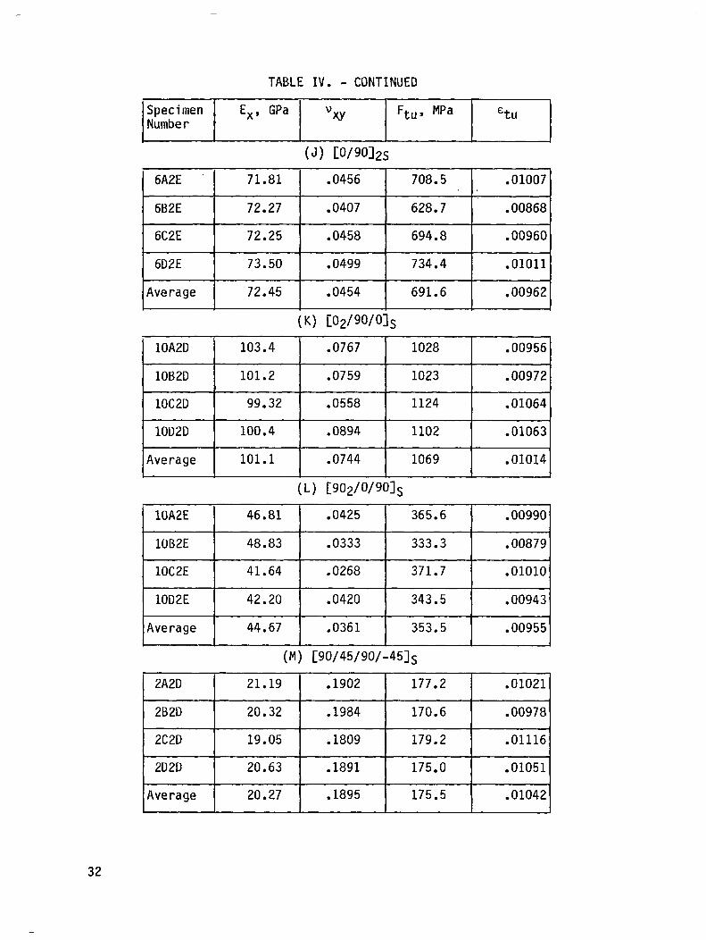
TABLE IV. - CONTINUED
Specimen E,, GPa Number
vxY Ftu, MPa &tu
I 6D2E I 73.50
IAverage I 72.45
(J> CWOlzs .0456 708.5 .01007
.0407 I 628.7 I .00868
I .0458 I 694.8 I .00960
.0499 I 734.4 I .OlOll
.0454 I 691.6 I .00962
(K) CO2/9O/Ols lOA2D 103.4 .0767 1028 .00956
lOB2D 101.2 .0759 1023 .00972
lOC2D 99.32 .0558 1124 .01064
lOD2D 100.4 .0894 1102 .01063
Average 101.1 .0744 1069 .01014
(L) c902/w901s
lOA2E 46.81 .0425 365.6 .00990
lDB2E 48.83 .0333 333.3 .00879
lOC2E 41.64 .0268 371.7 .OlOlO
lOD2E 42.20 .0420 343.5 .00943
Average 44.67 .0361 353.5 .00955
(Mj~ [90/45/90/-451s
32
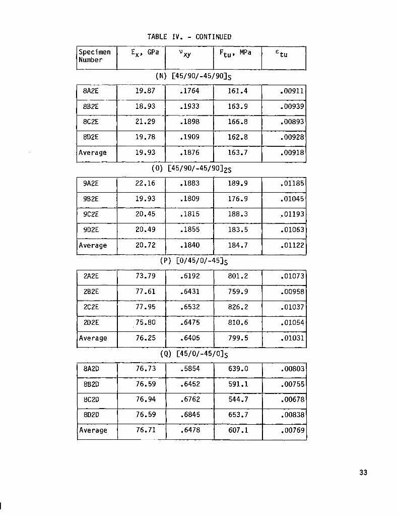
TABLE IV. - CONTINUED
Specimen Number
E x, GPa QY Ft,,, MPa EtU
(N) [45/90/-45/9O]s
8A2E I 19.87
--I .1764 161.4 .00911
.1933 163.9 .00939
.1898 166.8 .00893
.1909 162.8 .00928
.1876 163.7 .00918
(0) cww-w9012s
(V CW45/%4515
(Q) C45/%45/Ols
33
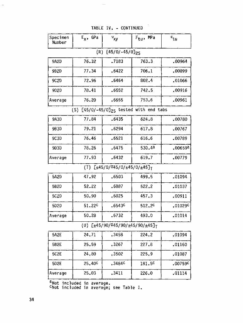
TABLE IV. - CONTINUED
Specimen E Number
x, GPa vxY Ftu, Mia %u
(R) [45/%45/012s
9A2D I
76.32 I
.7183 I
763.3 I
.00964
9B2D I
77.34 1 .6422 I
706.1 I
.00899
9C2D 72.96 .6464 802.4 .01066
9D2D 78.41 .6552 742.5 .00916
Average 76.20 .6655 753.6 .00961
(S) [45/O/-45/0]2S tested with end tabs
9A3D 77.84 .6435 624.8 .00780
9B3D 79.21 .6294 617.8 .00767
9C3D 76.46 .6521 616.6 .00789
9D3D 78.26 .6475 530.4a .00659a
Average 77.93 .6432 619.7 .00779
(T) [&45/0/945/0/&45/0/&45]T
5A2D 1 47.92 1 .6503 I 499.5 I .01094
5B2D 52.22 .6887 522.2 .01037
5C2D 50.90 .6825 457.3 .00911
5D2D I
51.22c I
.6543c I
512.2c I
.01029c
Average I
50.28 I
.6732 .01014
5A2E 24.71 .3458 224.2
5B2E 25.59 .3267 227.8
5C2E 24.80 .3502 225.9
5D2E 25.4Oc .3484c 181.5c
Average 25.03 .3411 226.0
aNot included in average. CNot included in average; see Table I.
.01094
.01160
.01087
.00759c
.01114
34
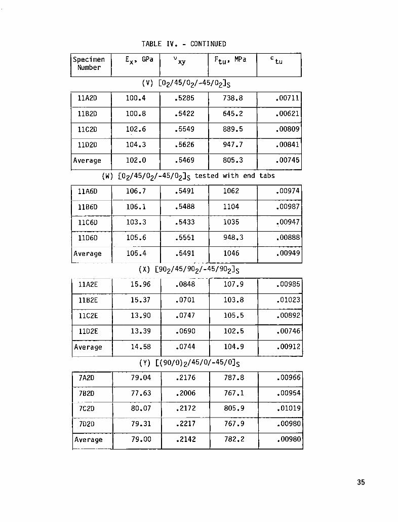
TABLE IV. - CONTINUED
Specimen E x, GPa vxY Ftu, MPa &tu Number
(v) ~02/45/02/-45/021s
llA2D 100.4 .5285 738.8 .00711
llB2D 100.8 .5422 645.2 .00621
llC2D 102.6 .5549 889.5 .00809
ilD2D 104.3 .5626 947.7 .00841
Average 102.0 .5469 805.3 .00745
(W) [02/45/02/-45/02]S tested with end tabs
106.7 .5491 1062 .00974
106.1 .5488 1104 .00987
p&i--I -103.3 .5433 1035 ,00947 -. .----.
llD6D 105.6 .5551 948.3 .00888
Average 105.4 .5491 1046 .00949
(X) c~~~/~~/~~~/-~~/~~~l~ llA2E 15.96 .0848 107.9 .00985
llB2E 15:37 .0701 103.8 .01023
k2E 13.90 .0747 105.5 .00892
llD2E 13.39 .0690 102.5 .00746
pe-Fi;e .I 14.58 .0744 104.9 .00912
(Y) [~90/0)~/45/0~-4~/~1~
7A2D 79.04 .2176 787.8 .00966
--7B2D 77.63 .2006 767.1 .00954
7C2D 80.07 .2172 805.9 .01019
-- 7D2D 79.31 .2217 767.9 .00980
Average 79.00 .2142 782.2 .00980
35
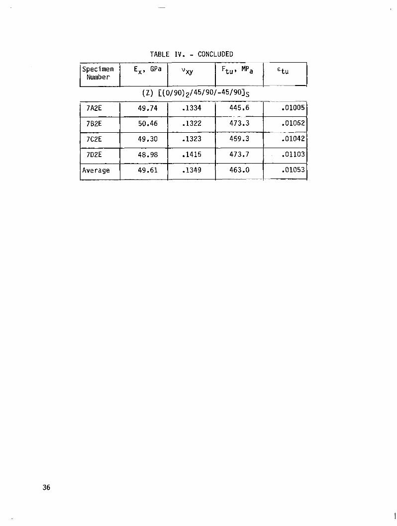
TABLE IV. - CONCLUDED
Specimen E x, GPa v'xY Ftus MPa Number
(Z) [(O/90) 2/45/90/-45/9Ols
3U il .01005
7B2E 50.46 .1322 473.3 .01062
I 7C2E I
49.30 1 .1323 ( 459.3 1 .01042
)iE 1 48.98 1 .1415 1 473.7 1 .01103 I I I r
Average 49.61 .1349 I 463.0 .01053
36
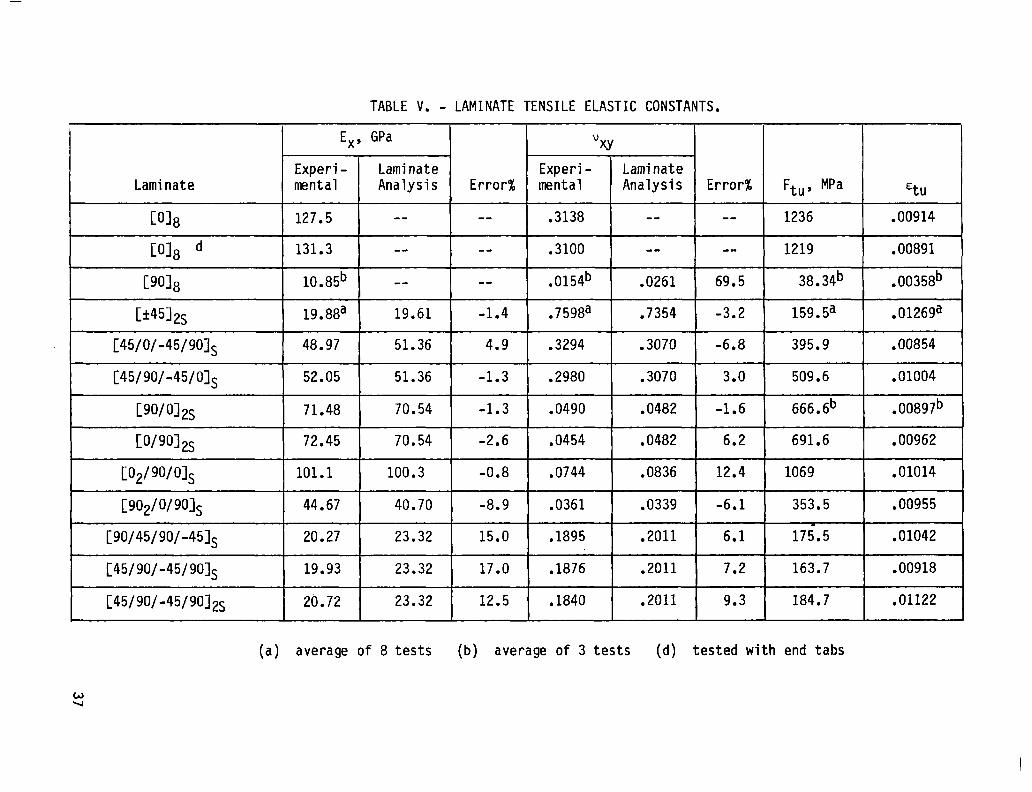
TABLE V. - LAMINATE TENSILE ELASTIC CONSTANTS.
Laminate
co18
co18 d
[go18
[*451pj
[45/O/-45/90&
[45/90/-45101s
CWQS
cw9012s
co,/ go/ 01s
[9O,/W9Ols
[90/45/90/-45]s
[45/90/-45/9O]s
[45/90/-45/90]2s
E x, GPa vxY
Experi- Laminate Experi- Laminate mental Analysis Error% mental Analysis Error% Ftu, MPa %U
127.5 -- -- .3138 -- -- 1236 .00914
131.3 -- -- .3100 -- -- 1219 .00891
10.85b -- -- .0154b .0261 69.5 38.34b .00358b
19.88a 19.61 -1.4 .7598a .7354 -3.2 159.5a . 0126ga
48.97 51.36 4.9 .3294 .3070 -6.8 395.9 .00854
52.05 51.36 -1.3 .2980 .3070 3.0 509.6 .01004
71.48 70.54 -1.3 .0490 .0482 -1.6 666.6b . 00897b
72.45 70.54 -2.6 .0454 .0482 6.2 691.6 .00962
101.1 100.3 -0.8 .0744 .0836 12.4 1069 .01014
44.67 40.70 -8.9 .0361 .0339 -6.1 353.5 .00955
20.27 23.32 15.0 .1895 .2011 6.1 175.5 .01042
19.93 23.32 17.0 .1876 .2011 7.2 163.7 .00918
20.72 23.32 12.5 .1840 .2011 9.3 184.7 .01122
(a) average of 8 tests (b) average of 3 tests (d) tested with end tabs
CA U
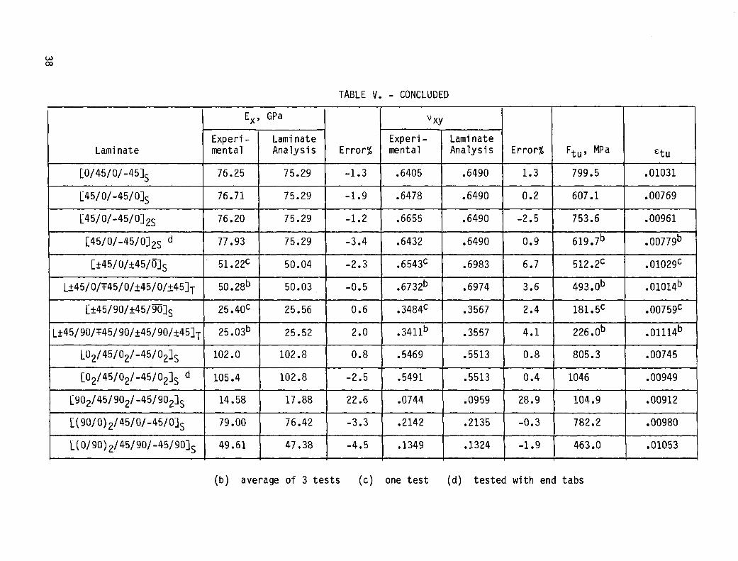
TABLE V. - CONCLUDED
E x, GPa v'xY
Experi- Laminate Experi- Laminate Laminate mental Analysis Error% mental Analysis Error% Ftu, MPa 3U
c0/45/0/-4515 76.25 75.29 -1.3 .6405 .6490 1.3 799.5 .01031
c45/o/-45/035 76.71 75.29 -1.9 .6478 .6490 0.2 607.1 .00769
L45/O/-45/O]2s 76.20 75.29 -1.2 .6655 .6490 -2.5 753.6 .00961
[45/0/-45/012s d 77.93 75.29 -3.4 .6432 .6490 0.9 619.7b .00779b
[f45/0/f45/0]S 51 .22c 50.04 -2.3 .6543c .6983 6.7 512.2c .0102gc
L+45/0/r45/0/+45/0/+45]T 50.28b 50.03, -0.5 .6732b .6974 3.6 493.0b .01014b
[+45/90/+45/x$ 25.40c 25.56 0.6 . 3484c .3567 2.4 181.5c .00759c
L+45/90/r45/90/+45/90/+451T 25 .03b 25.52 2.0 .3411b .3557 4.1 226 .Ob .01114b
&/45/02/-45/02& 102.0 102.8 0.8 .5469 .5513 0.8 805.3 .00745
[0#5/02/-45/02& d 105.4 102.8 -2.5 .5491 .5513 0.4 1046 .00949
s902/45/90,/-45/902]s 14.58 17.88 22.6 .0744 .0959 28.9 104.9 .00912
s(9o/0),/45/0/-45/01s 79.00 76.42 -3.3 .2142 .2135 -0.3 782.2 .00980
1(0/90),/45/90/-45/90$ 49.61 47.38 -4.5 .1349 .1324 -1.9 463.0 .01053
(b) average of 3 tests (c) one test (d) tested with end tabs
ia
t
Transverse direction
k-940 mm-4
~~\\'\\""""""""""""""' NXlA
hlYI)A N
Fiber direction 4Y
\
i
Specimen type
(A,B,C,D,E)
Specimen position
IX1
!
L .Laminate number
(2,3 ,...,12)
N
I -Sheet (A,B,C,D)
Specimen code
Longitudina
L,
1 direction
Figure 1. - Specimen layout and numbering system.
39

1000 -
800 -
rcI 9 600 - m x
b
el
G aJ L 2: 400 -
-polynomial fit
0 .005 .OlO .015
Strain
Figure 2. - Stress-strain curve for specimen 2A2E.
1500 -
1000 -
-Average polynomial fit 0 12A2D IJ 12B2D
12C2D 12D2D
Strain
Figure 3. - Stress-strain curve for [D], laminate,
1500 -
1000 -
-Average polynomial fit
g E; A - x 12C6D , 12D6D
Strain
Figure 4. - Stress-Strain curve for [D], laminate tested with end tabs,
-Average polynomial fit 0 12A2E 0 12B2E
12C2E 12D2E
0 .-I II II II I I IIIIIlll lllllllll llllllIII lllllllll lllllllll -.OOl 0 .OOl .002 .003 .004 .005
Strain
Figure 5. - Stress-strain curve for [go]8 laminate!
n x
b
150 -
100 -
50 - -Average polynomial fit
Strain
Figure 6. - Stress-strain curve for [k45]2s laminate.
n x
b
200
150
100
50
0
-Average polynomial fit
0
Strain
.005 .OlO ,015
Figure 7. - Stress-strain curve for [k45]2s laminate,
L x b
1 200,
t
t i-- 1 ;3 0 iI
-.OlO
-Average polynomi al
Strain
fit
Figure 8. - Stress-strain curve for [45/O/-45/901s laminate.
600 -
-Average polynomial fit
P q 4B2E 4C2E 4D2E
Strain
Figure 9. - Stress-strain curve for [45/90/-45/Ols laminate,
800
600
400
200
8.002 0 .002 .004 .006 .008 .OlO .012
Strain
Figure 10. - Stress-strain curve for [90/O]2s laminate.
800 -
600 -
200 -
0lZLJ-L -.002 ,004 .006 .008 .OlO .012
Strain
Figure 11. - Stress-strain curve for [0/9O],S laminate.

1500 -
1000 -
Ia 52
a x b
UY z L =I
500 -
I I I I I I I I I
-.OlO -.005 0 .005 .OlO
Strain
-Average 0 lOA2D
Y 0 lOB2D
polynomial fit
.015
Figure 12. - Stress-strain curve for [0,/9O/OJ, laminate.
-Average polynomial fit 0 lOA2E q lOB2E 2 lOC2E
lOD2E
I I I I I I I I I I I I I 11 1 11 1 I I 11 j I 11 1 .002 .004 .006 .008 .OlO .012
Strain
Figure 13. - Stress-strain curve for [902/O/90Js laminate.
“Y
150 -
100 -
50 -
O-1 1 I IIL -.005
-Average polynomial fit
? n 2D2D
I II I I I I I I 11 III Ill II I ll111II l I 0 .005 .OlO .015
Strain
Figure 14. - Stress-strain curve for [90/45/90/-451, laminate.
1: 750'
100 -
50 -
OFI1 11 -.005
III 0 ,005
Average polynomial fit 8A2E 8B2E 8C2E 8D2E
III II 1 III1 I1 1 l l .OlO .015
Strain
Figure 15. - Stress-strain curve for [45/90/-45/9OJ laminate.
200 F
150
100
50
0
1 k n/
EY
-Average polynomial fit
q 9B2E 9C2E
.005
Strain
.OlO .015
Figure 16. - Stress-strain curve for [45/90/-45/90]2s laminate.
1000 -
800 -
200 -
0
-Average polynomial fit 0 2A2E j-J 2B2E O2C2E
Strain
Figure 17. - Stress-strain curve for [O/45/0/-451s laminate.
600
200
/
-Average polynomial fit
Strain
Figure 18. - Stress-strain curve for [45/O/-45/Ols laminate.
7000 -
800 -
g 600 -
lx
u; i =I 400 -
-Average polynomial tit
Strain
Figure 19. - Stress-strain curve for [45/O/-45/O]2s laminate.
1000 -
800 -
600 -
400 -
200 -
r- 0
Fi gure 20. - Stress-strain curve for [45/0/-45/O],, laminate tested with end tabs.
-.OlO -.005
Average polynomial fit 0 9A3D 0 9B3D
9C3D 9D3D
IIIIIllllIlllIIIIIIIIIIIII,~ .uu5 .UlU
Strain
-
600
-Average 0 5A2D Cl 5B2D 2 5C2D
5D2D
I I I I I I I I I I I
polynomial fit
I I I I I I I I I .005 .070 .015
Strain
Figure 21. - Stress-strain curve for [~45/O/t45/?lS and [+45/O/i45/O/+45/O/z45]T laminates.
250
E 200 -
CrJ 52 150 -
b--X e
2 i!! =I 100 -
50 -
0 I-L
-Average polynomial fit
A 5D2E
.005
Strain
.OlO .015
Figure 22. - Stress-strain curve for [+45/90/+45/Bjs and [+45/90/i45/90/+45/90/f45]T laminates.
* 2 i?! =I
500 -
0 IIIIIII -.OlO
-Average po 0 ll‘A2D 0 llB2D
Strain
lynomial fit
I I I I I I I ,015
Figure 23. - Stress-strain curve for [02/45/02/-45/02JS laminate.
1000 0 P
3 "
: 2! s
500
- Average polynomial fit
0 .005 .070 .015
Strain
Figure 24. - Stress-strain curve for [02/45/02/-45/02]s laminate tested with end tabs,
-Average polynomial fit 0 llA2E 0 llB2E
-.002 0 .002 .004 .006 .008 ,010 ,012
Strain
Figure 25. - Stress-strain curve for [90,/45/90,/-45/902]S laminate,
1000
i 800
600
-Average polynomial fit
Strain
Figure 26. - Stress-strain curve for [(90/0),/45/0/-45/O], laminate,
- Average polynomial fit
E :E
2 7C2E 7D2E
1 IIll I I l I I I I I I I I I Illllll I I 0 .005 .OlO .015
Strain
Figure 27. - Stress-strain curve for [(O/90)2/45/90/-45/90]s laminate.
.OlO X w
; *r E 3:
.005
(Eta,& GPa
- polynomial deri vative curve
0 .2 .4 .6 .8 1.0
ve curve
50 100 150
Figure 28. - Tangent modulus and Poisson's ratio for specimen 2A2E.
66
.015
.OlO
1
.005
I
0
oi12A2D q 12B2D 0,12C2D A12D2D
- Average polynomial derivative curve
-L
(Eta,.& GPa
0.12A2D q 12B2D
'0,12C2D A12D2D
- Average polynomial derivative-curve
u 'I&I I I@ I I I I I I I I I I c? I I I I I I I I I I I I I I 0 .2 .4 .6 .8 1.0
(v 1 tan xy
Figure 29. - Tangent modulus and Poisson's ratio for [O], laminate.
67
; -F tu L
=: .005
0
012A6D El q 'l2B6D 0]12C6D Al2D6D
0 A
- Average polynomial 4 derivative curve Q
~iiirii~i I I I I I I I I I IRI R IE
(EtanJx, GPa
012A6D '~12B6D 012C6D A12D6D
- Average deriva
0 .2 .4 .6 .8 1.0
Iv 1 tan xy
polynomial tivii curve
Figure 30. - Tangent modulus and Poisson's ratio for [O], lami-nate tested with end tabs.
68
A
012A2E q 12B2E 012C2E A l?D2E
- Average polynomial derivative curve
(EtanIx, GPa
.005
.004
0 lc A
A W x .003
2 -C 2 =I
.002
A
OA
.OOl
0
A O 0
0 cl
012A2E q 12B2E 012C2E A12D2E
- Average polynomial derivative curve
13 , RIIIIII IIIIIIIIIIIIIIILnllIl IIIIIIIl II Ill III III
.2 .4 .6 .8 1.0
(v 1 tan xy
Figure 31. - Tangent modulus and Poisson's ratio for [go], laminate.
69
0
o3A2D q 3B2D 0;3C2D A:3D2D
- Average polynomial derivative curve
50 100 150
(Et-n Ix 3 GPa
o 3A2D q ;3B2D 013C2D A 3D2D
- Average polynomial derivative curve
B A
.4 .6 .8 1.0
(v > tan xy
Figure 32. - Tangent modulus and Poisson's ratio for [H15]2s laminate.
70
o.3A2E q 3B2E o3C2E A3D2E
-'Average polynomial derivative curve
lFblllllllllllll1 I l I l l l ll[
50 100 150
(Eta,.Jxs GPa
.015 F I
.OlO
I .005
1
o 3A2E 0 3B2E o3C2E A 3D2E
- Average polynomial derivative curve
I I I I I I I I I I I I I I I I I I I I I I I I I I I I
0 .2 .4 .6 .8 1.0
(V i tan xy
Figure 33. - Tangent modulus and Poisson's ratio for [~k45]~~ laminate.
71
.015
.OlO X w
2 F 2 x
.005
I LJ 11
o 4B2D q 4C2D 0 4D2D A 4A2E
-Average polynomial derivative curve
I I I I I
(Etan lx, GPa
.015
.OlO x W
; V-
z
3:
.005
0 0 0 4B2D 'o 4C2D 0 4D2D A 4A2E
-Average polynomial derivative curve
I I I I I
0 .2 .4 .6 .8 1.0
("tan)xy
Figure 34. - Tangent modulus and Poisson's ratio for [45/O/-45/901s laminate.
72
> 04A2D
I q 4B2E
$ 04C2E *4D2E
, - Average polynomial derivative curve
I :
IAI I I I I I I I I I I I I I I I
(Eta,Jxs GPa
r -
a 0 4A2D 0 4B2E 0,4C2E A 4D2E
B - Average polynomial
derivative curve
0 .2 .4 .6 .8 1.0
(v 1 tan xy
Figure 35. - Tangent modulus and Poisson's ratio for [45/90/-45/O]s laminate.
73
0 o 6A2D 0 0 0 6B2D
o6C2D A 6D2D
- Average polynomial derivative curve
.OlO X
W
; *r
E!
=: .005
(Etan)xs GPa
o 6A2D q 6B2D o6C2D
a A6D2D
- Average polynomial I
0. 0 derivative curve
i 0
II IlIIIIllI IIIIlIIII IIIIIIIII IIIIIIIII
0 .2 .4 .6 .8 1.0
Figure 36. - Tangent modulus and Poisson's ratio for [90/O],, laminate.
74
.015
.OlO X
W
cl -F I8 L
=: .005
~ 0
I .I -_I I J I I _I 1 I
50
0 6A2E 17 6B2E 06C2E A 6D2E
- Average polynomial derivative curve
I I I I
(EtanIx 3 GPa
, 0 6A2E L 17 6B2E
e 06C2E A6D2E
-Average polynomial derivative curve-
0 I7 I I ??I I I ”
l$i&i+ I l I---& U I.l.llJ~l
-. 2 0 .2 .4 .6 .8 1.0
(v ) tan xy
Figure 37. - Tangent modulus and Poisson's ratio for [O/90],, laminate.
75
.015 r- L
.OlO - X w
; *r 2 z
.005 -
I I I I I I I I I I I I I I I I I
0
.015
0 lOA2D 0 lOB2D 0 lOC2D A lOD2D
-Average polynomial > derivative curve
50 100 150
(EtanIx GPa
o lOA2D q ,lOB2D
E ollOC2D ahOD2D
- Average polynomial derivative curve
0 .2 .4 .6 .8 1.0
(v 1 tan xy
Figure 38. - Tangent modulus and Poisson's ratio for [0,/90/O], laminate.
76
o lOA2E q lOB2E 0 lOC2E
*a$!i?iF ” o$ A lOD2E 0 -Average polynomial
derivatiG$ curve
I I I I I I I I I I I I I I I I I I
0 50 .' 100 150
(EtanIx, GPa
.015
1
o lOA2E 0 •I lOB2E
0 lOC2E 0 A lOD2E
- Average polynomial derivative curve
-. 2 b .2 .4 .6 .8 1.0
(v 1 tan xy
Figure 39. - Tangent modulus and Poisson's ratio for [90,/O/90], laminate.
77
I
o 2A2D q 2B2D o 2C2D A 2D2D
-Average po derivati
lynomial ve curve
LLdLuLLIiIIII 50 100 150
(Eta,& GPa
.015 F
,010 x w "
s SF l-6 L L) O I in
o 2A2D q 2B2D 012C2D A 2D2D
- Average polynomial derivative curve
0 .2- .4 .6 .8 1.0
b 1 tan xy .
Figure 40. - Tangent modulus and Poisson's ratio for [90/45/90/-45]S laminate.
78
L-L
o 8A2E q 8B2E 0 8C2E .A 8D2E
- Average polynomial derivative curve
I I I I
(Eta,.&, GPa
8 %
o 8A2E 0 q 8B2E
o 8C2E i A 8D2E
- Average polynomial derivative ctirve
Ill I I1,,,,,,1,,,,,,,,, 0 .2 .4 .6 .8 1.0
(v 1 tan xy
Figure 41. - Tangent modulus and Poisson's ratio for [45/90/-45/901S laminate.
79
0
.015
! '
o 9A2E q 9B2E 0 9C2E A 9D2E
L- Average polynomial derivative curve
Il~Al’ll”“” 1”“““’
50 100 150
(Eta& GPa
A 0 9A2E 0 9B2E 0 9C2E
> A 9D2E - Average polynomial
derivative curve
, II IIIII~II II IIIIIII III1 III’1 I ‘1 ‘11 ’ 1 l
0 .2 .4 .6 .8 1.0
(v 1 tan xy
Figure 42. - Tangent modulus and Poisson's ratio for [45/90/-45/90]2S laminate.
80
0 2A2E 0 2B2E 0 2C2E * 2D2E
- Average polynomial
~~,',',,',",', derivative curve
(Eta,& GPa
.OlO X
W
; SF-
E’
=: .005
0 2A2E q 2B2E 0 2C2E A 2D2E
- Average polynomial derivative curve
.4 .6 .8 1.0
b 1 tan xy
Figure 43. - Tangent modulus and Poisson's ratio for [O/45/0/-45JS laminate.
81
.015
! ,010 k-
WX L-
2 -I- r- E
I- l-
=: I-
.005
8A2D 8B2D 8C2D 8D2D Average polynomial
derivative curve
(Eta,.& GPa
,010 X
W f
.6 .8
('tan)xy
-8A2D 8B2D 8C2D 8D2D Average po
derivati lynomial ve curve
Figure 44. - Tangent modulus and Poisson's ratio for [45/0/-45/O], laminate.
82
I I I I L
0 9A2D 0 9B2D 0 9C2D A 9D2D
- Average polynomial deriva tive curve
I I IA’
(Etan&, GPa
9A2D '9B2D 9C2D 9D2D Average polynomial
derivative curie-
0 .2 .4 .6 .8 1.0
('tan)xy
Figure 45. - Tangent modulus and POiSSOn's ratio for [45/D/-45/O]2S laminate.
83
---. I I
0 9A3D 0 9B3D 09C3D A 9D3D
-Average polynomial derivative curve
Id 150
(Eta& GPa
.015
.OlO X w / \
o 9A3D q 9B3D o 9C3D A 9D3D
-Average polynomial derivative curve
.4 .6- .8 1.0
(v ) tan xy
84
Figure 46. - Tangent modulus and Poisson's ratio
for [45/0/-45/O]2s laminate tested with end tabs.
o 5A2D u 5B2D 0 5C2D * 5D2D
- Average polynomial derivative curve
I I I I I I I I I I I I I I I I
(Eta,.& GPa
q
o 5A2D 3 q 5B2D
o5C2D I A 5D2D
- Average polynomial ~i,,.,,,,~rivative curve
0 .2 .4 .6 .8 1.0
(Vtan)xy
Figure 47. - Tangent modulus and Poisson's ratio for [f45/0/f45bJJS and [f45/O/i45/O/+45/O/+45]T laminates.
85

1.-L
0 50
(Eta,& GPa
II 100
t 0 -I
I I llJ,ll Id
0 5A2E q 5B2E 0 5C2E A 5D2E
- Average polynomial derivative curve
u 1 ~.lJ 150
o 5A2E q 5B2E o 5C2E A 5D2E
- Average polynomial derivative curve
.4 .6 .8 1.0
(v 1 tan xy
Figure 48. - Tangent modulus and Poisson's ratio
for [f45/90/f45/XWJS and [+45/9O/i45/90/+45/90/+45]T laminates.
86
llA2D llB2D llC2D llD2D Average polynomial
dwivative curve
(EtaJx3 GPa
0 .4 - .5
b 1 tan xy
0 llA2D 0 llB2D 0 llC2D A 11020
- Average polynomial derivatfve curve
,~,I’ IIlIIIIII
.8 1.0
Figure 49. - Tangent modulus and Poisson's ratio
for [02/45/02/-45/02& laminate.
87
.015 F
; -r
2
=5 .005
<,,‘,“, 1 -Average polynomial derivative curve
I I I I I I I I
0 50 100 150
(Et-n)x, GPa
o llA6D q llB6D 0 llC6D A llD6D
- Average polynomial de-rivative curve
0 .2 .4 .6 .8 1.0
(v 1 tan xy
Figure 50. - Tangent modulus and Poisson's ratio
for [02/45/02/-45/02]S laminate tested with end tabs.
88
.OlO WX
; -r
2
x
.005
A o llA2E
0 q llB2E 0 llC2E
I7 A llD2E - Average polynomial
derivative curve
I I I I I I I I I I I I I I I I I I I I I I I I
(Etan)xv GPa
.015
.OlO WX
0 .2 .4 .6 .8 1.0
o llA2E q llB2E 0 llC2E A llD2E
-Average polynomial derivative curve
b 1 tan xy
Figure 51. - Tangent modulus and Poisson's ratio
for [902/45/902/-45/902]S laminate.
89
b&O
A0 0 005 - 0, t
4
0
0 0 q o 7A2D
a 0 0 7B2D 0 7C2D A 7D2D
- Average polynomial derivative curve
+I $ “0 pn 0 0 7A2D 7B2D
0 7C2D ) A 7D2D
- Average polynomial derivative.c%rGe
I’~“‘IIIr~llPIIIIrlrllIIlIIllrIllrIlI
0 .2 .4 .6 .8 1.0
('tan)xy
Figure 52. - Tangent modulus and Poisson's ratio for [(90/0),/45/0/-45/O], laminate.
90
.OlO - X w
; -I-- E z
.005 -
I I I I I I
0
o 7A2E 0
I 7B2E
- 0 7C2E A 7D2E
Average polynomial
; derivative curve
LLugLL_LuI 50 100 150
(Etan)xs GPa
0 .2 .4 .6 .8 1.0
o 7A2E q 7B2E o'7C2E A 7D2E
- Average polynomial derivative curve
(v > tan xy
Figure 53. - Tangent modulus and Poisson's ratio
for [(O/90)2/45/90/-45/90]S laminate.
91
E,, GPa
‘00
E,, GPa
Figure 54. - Cordell plot of Young's modulus, E,.
.6
v*Y 3
3
0
.6
m4 vxY
92
0
Figure 55. - Cordell plot of Poisson's ratio, vxy.
Ftll’ MPa
.
. ‘000
.‘ Ft”’ MPa
Figure 56. - Cordell plot of ultimate tensile strength, Ftu.


![Effect of corrosive solutions on composites laminates ......Stamenovic et al [1] compared, for glass/polyester composites, the effect of alkaline and acid solutions on their tensile](https://img.dokumen.tips/doc/110x75/5fe48274691d776b027d3286/effect-of-corrosive-solutions-on-composites-laminates-stamenovic-et-al-1.jpg)