Embed Size (px)
Citation preview

NASA Contractor Report 3871
Accelerated Viscoelastic
Characterization of T300/5208
Graphite-Epo_w Laminates
M. E. Tuttle and H. F. Brinson
COOFERATiVE AGREEMENT NCC2-71
MARCH 1985
N SA
https://ntrs.nasa.gov/search.jsp?R=19850012961 2019-09-09T15:52:45+00:00Z

NASA Contractor Report 3871
Accelerated Viscoelastic
Characterization of T300/5208
Graphite-Epoxy Laminates
M. E. Tuttle and H. F. Brinson
Virginia Polytechnic Institute and State University
Blacksburg, Virginia
Prepared for
Ames Research Center
under Cooperative Agreement NCC2-71
NILS/XNational Aeronautics
and Space Administration
Scientific and TechnicalInformation Branch
1985
ACCELERATED VISCOELASTIC CHARACTERIZATION
OF T300/5208 GRAPHITE-EPOXY LAMINATES
(ABSTRACT)
The viscoelastic response of polymer-based composite
laminates, which may take years to develop in service, must
De anticipated and a_u_LLodated at _ __ _
Accelerated testing is therefore require_ to allow long-term
compliance predictions for composite laminates of arbitrary
layup, based solely upon short-term tests.
In this study, an accelerated viscoelastic
characterization scheme is applied to T300/5208 graphite-
epoxy laminates. The viscoelastic response of
unidirectional specimens is modeled using the theory
developed by Schapery. The transient component of the
viscoelastic creep compliance is assumed to follow a power
law approximation. A recursive relationship is developed,
based upon the Schapery single-integral equation, which
allows approximation of a continuous time-varying uniaxial
load using discrete steps in stress.
The viscoelastic response of T300/5208 graphite-epoxy at
149C to transverse normal and shear stresses is determined

using 90-deg and 10-deg off-axis tensile specimens,
respectively. In each case the seven viscoelastic material
parameters required in the analysis are determined
experimentally, using a short-term creep/creep recovery
testing cycle. A sensitivity analysis is used to select the
appropriate short-term test cycle. It is shown that an
accurate measure of the power law exponent is crucial for
accurate long-term predictions, and that the calculated
value of the power law exponent is very sensitive to slight
experimental error in recovery data. Based upon this
analysis, a 480/120 minute creep/creep recovery test cycle
is selected, and the power law exponent is calculated using
creep data. A short-term test cycle selection procedure is
proposed, which should provide useful guidelines when other
viscoelastic materials are being evaluated.
Results from the short-term tests on unidirectional
specimens are combined using classical lamination theory to
provide long-term predictions for symmetric composite
laminates. Experimental measurement of the long-term creep
compliance at 149C of two distinct T300/5208 laminates is
obtained. A reasonable comparison between theory and
experiment is observed at time up to 105 minutes.
Discrepancies which do exist are believed to be due to an
insufficient modeling of biaxial stress interactions, to the
accumulation of damage in the form of matrix cracks or
ii

voids, and/or to interlaminar shear deformations which may
occur due to viscoelastic effects or damage accumulation.
iii
Acknowledgements
The authors are indebted to many individuals who have
helped make this work possible. Special acknowledgement is
appropriate for the financial support of the National
Aeronautics and Space Administration through Grant NASA_CC2-
71. The authors are grateful to Dr. H.G. Nelson of NASA-
.Ames for his support and many helpful discussions. The
previous work of Drs. Y.T. Yeow, W.I. Griffith, D.A.
Dillard, C. Hiel. and S.C. Yen while at VPI&SU relative to
the viscoelastic response of composites is gratefully
acknowledged. The technical support of Mr. M. Rochefort,
Mr. B. Barthelemy, and Mr. M. Zhang is also acknowledged.
The authors are especially indebted to Mrs. Peggy Epperly
for typing the equations and Ms. Catherine Brinson for
inking the figures.
iv
TABLEOF CONTENTS
ABSTRACT...........................
ACKNOWLEDGEMENTS.......................
LIST OFFIGURES .......................
I. INTRODUCTION.....................
Previous Research at VPI&SU ............
Objectives of Present Study ............
II. BACKGROUNDINFORMATION................
The Theory of Viscoelasticity ...........
Linear Viscoelasticity .............
Nonlinear Viscoelasticity ............
Classical Lamination Theory ............
III. THESCHAPERYNONLINEARVISCOELASTICTHEORY ......
The Schapery Viscoelastic Model ..........
Experimental Measurementof the SchaperyParameters .....................
Program SCHAPERY................
Program FINDLEY.................
Average Matrix Octahedral Shear Stress .......
Lamination Program VISLAP .............
IV. SENSITIVITYANALYSIS .................
Impact on Long-Term Predictions ..........
Sensitivity to Experimental Error .........
Linear Viscoelastic Analysis ..........
Nonlinear Viscoelastic Analysis .........
PAGE
i
iv
viii
i
5
19
23
23
32
40
52
64
64
77
79
85
85
89
94
97
105
ii0
116
V
Vo
VI.
VII.
Summary of the Sensitivity Analysis ........
SELECTION OF THE TESTING SCHEDULE ...........
Preliminary Considerations .............
Testing Schedule Selected .............
Proposed Test Selection Process ..........
ACCELERATED CHARACTERIZATION OF T300/5208 .......
Specimen Fabrication ................
Equipment Used ...................
Selection of Test Temperature ...........
Tests of 0-deg Specimens ..............
Tests of 90-deg Specimens .............
Analysis Using Creep Data ............
Analysis with Uncorrected Recovery Data .....
Analysis with Recovery Data Corrected Using
Method 1 ....................
Analysis with Recovery Data Corrected Using
Method 2 ....................
Calculation of the Nonlinear Parameters .....
Tests of 10-deg Specimens .............
Linear Analysis .................
Nonlinear Analysis ...............
LONG TERM EXPERIMENTS .................
Selection of the Laminate Layups ..........
Drift Measurements .................
Specimen Performance ................
Page
122
124
124
126
132
134
134
139
142
143
145
156
158
160
162
169
174
179
180
186
186
190
192
vi

Vlll. COMPARISONBETWEENPREDICTIONANDMEASUREMENT.....
IX. SUMMARYANDRECOMMENDATIONS..............
Summaryof Results .................
Recommendations ..................
REFERENCES..........................
Page
194
205
205
209
213
vii
LIST OF FIGURES
Figure
i.i
1.2
1.3
1.4
1.5
2.1
2.2
2.3
2.4
2.5
2.6
2.7
Flow chart of the proposed procedures for laminate
accelerated characterization and failure
prediction [23] ..................
Comparison of predicted and experimental creep
compliance for laminate K ([30/-6014s) at 320°F
(160°C) ......................
Power law parameters for laminate K ([30/-6014s)
at 320°F (160°C) ..................
Creep ruptures of K specimens ([-30/6014s) at
320°F (1600C) ...................
Current accelerated characterization procedure
used at VPI&SU ...................
Stress and strain histories for a creep/creep
recovery test ...................
Strain and stress histories for a stress relaxation
test .......................
Strain and stress histories for a constant strain
rate test .....................
Typical creep/creep recovery behaviour for visco-
elastic solids and viscoelastic fluids .......
Isochronous stress-strain curves illustrating
linear and nonlinear viscoelastic behaviour ....
Simple mechanical analogies used to model visco-
elastic behaviour ................
Typical viscoelastic response for a Kelvin element;o o
t = i, k - i ..................
Generalized viscoelastic models ..........
Schematic representation of a typical retardation
spectrum ....................
13
14
16
18
25
26
27
29
31
33
35
36
38
viii
Fisure
2.10
2 .ii
2.12
2.13
J.5
3.6
4.1
4.2
4.3
4.4
4.5
4.6
4.7
Approximation of an arbitrary stress history using
a series of discrete steps in stress ........
TTSP formation process as given by Rosen [i] ....
Ply orientation for a [0/9012 s composite laminate
Coordinate systems used to describe a composite
laminate ......................
Two-step uniaxial load history ...........
Approximation of ply stress history using discrete
steps in stress ..................
Flow chart for program SCHAPERY - linear analysis
Flow chart for program SCHAPERY - nonlinear
analysis ......................
.L'J.UW ',-U-dt U J-U£ _J.LO_tdiil £ .LZ_.U,L,r'.I ...........
Flow chart for viscoelastic laminated composite
analysis, VISLAP ..................
Percent error in predicted creep strains due to+ 10% error in A or _A-- O vU " " " " • " ° " " " " " " "
Percent error in predicted creep strains due to a
+ 10% error in C, gl' or g2 ............
Percent error in predicted creep strains due to a
+ 10% error in n ..................
Percent error in predicted creep strains due to a
+ 10% error in a .................--
Recovery strain histories used in sensitivity
analysis for a constant + 10% error ........
Recovery strain histories used in sensitivity
analysis for a constant + 5 bin/in offset error
Sensitivity of power law parameters Ao, n, and C topercentage errors in creep strain data; stress =
1750 psi, actual Ao, n, and C values are 0.674,
0.33, and 0.0145, respectively ...........
Page
40
42
54
55
73
75
81
g3
86
91
I00
Iu-
102
103
107
109
iii
ix

Figure
4.8
4.9
4 .I0
4.11
4.12
4.13
4.14
4.15
4.16
4.17
4.18
Sensitivity of power law parameters, Ao, n, and C
to offset errors in creep strain data; stress =
1750 psi, actual Ao, n, and C values 0.674, 0.33,
and 0.0145, respectively ..............
Sensitivity of power law parameters C and n to
percentage errors in recovery strain data; stress
level = 1750 psi, actual C and n values are
0.0145 and 0.33, respectively ...........
Sensitivity of power law parameters C and n to
offset errors in recovery strain data; stress =
1750 psi, actual C and n values 0.0145 and 0.33,
respectively ....................
Sensitivity of go to percentage errors in strain
data; stress = 1750 psi, A o = 0.674, C = 0.0145,n = 0.33 ......................
Sensitivity of gl to percentage errors in strain
data; stress = 1750 psi, Ao = 0.674, C = 0.0145,n = 0.33 ......................
Sensitivity of g2 to percentage errors in strain
data; stress = 1750 psi, A o = 0.674, C = 0.0145,
n = 0.33 ......................
Sensitivity of ao to percentage errors in strain
data; stress = 1750 psi, Ao = 0.674, C = 0.0145,n = 0.33 ......................
Sensitivity of go to offset errors in strain
data; stress = 1750 psi, Ao = 0.674, C = 0.0145,
n = 0.33 ......................
Sensitivity of gl to offset errors in strain
data; stress = 1750 psi, A ° = 0.674, C = 0.0145,n = 0.33 ....................
Sensitivity of g2 to offset errors in strain
data; stress = 1750 psi, A o = 0.674, C = 0.0145,n = 0.33 .....................
Sensitivity of ao to offset errors in strain
data; stress = 1750 psi, Ao = 0.674, C = 0.0145,n = 0.33 .....................
Page
112
114
115
117
117
118
118
120
120
121
121
X
Fisure
5.1
5.2
6.1
6.2
6.3
6_4
6.5
6.6
6.7
6.8
6.9
6 .i0
6 .ii
6.12
Transient creep response predicted for a creep
stress of 12.1 MPa (1750 psi); Ao = 0.674,C = 0.0145 .....................
Predicted recovery response following 480 minutes
of creep at 12.1 MPa (1750 psi); Ao = 0.674,C = 0.0145 .....................
10-deg off-axis tensile specimen, indicating
orientation of the 3-element strain gage rosette
Five minute creep compliance and average creep
rate for T300/5208; stress = 11.4 MPa .......
480/120 minute creep/creep recovery data set and
analytic fit, plotted using the interactive
graphics routine ..................
plotted using the interactive graphics routine
120 minute recovery data and analytic fit, plotted
using the interactive graphics routine .......
Stress-strain curves obtained at 0.5 and 480
minutes _ qn__=g T300/_on_ opecimens .......
Permanent strains recorded following the 480/120
minute creep/creep recovery tests using 90-deg
T300/5208 specimens ................
Values obtained for the linear viscoelastic
parameters Ao, C, and n using the program FINDLEY
Values obtained for the linear viscoelastic
parameters A , C, and n using the program SCHAPERYo
and uncorrected recovery data ...........
Values obtained for the linear viscoelastic
parameters Ao, C and n using the program SCHAPERY
and recovery data corrected using method 1 .....
Comparison of expected recovery curve at 15.6 MPa
(2263 psi) based on creep data and measured recovery
data corrected using method 1 ...........
Comparison of expected recovery curve at 15.6 MPa
(2263 psi) based on creep data and measured
recovery data corrected using method 2 .......
130
131
138
144
148
149
150
IgO.L -# _-
155
157
159
161
163
165
xi
Figure
6.13
6.14
6.15
6.16
6.17
6.18
6.19
6.20
7.1
7.2
8.1
8.2
Values obtained for the linear viscoelastic
parameters Ao, C, and n using the program SCHAPERYand recovery data corrected using method 2 .....
Values obtained for go and gl as functions ofapplied stress and of the average octahedral shear
stress .......................
Values obtained for g2 and ao as functions of
applied stress and of the average matrix octahedral
shear stress ....................
Stress-strain curves obtained at 0.5 and 480
minutes for 10-deg T300/5208 specimens .......
Permanent strains recorded by gages a, b, and c
following the 480/120 minutes creep/creep recovery
tests using lO-deg off-axis T300/5208 specimens
Values obtained for go and gl as functions ofapplied shear stress and of average matrix
octahedral shear stress ..............
Values obtained for g2 as a function of applied
shear stress and of the average matrix octahedral
shear stress ....................
Values obtained for ao as a function of appliedshear stress and of the average octahedral shear
stress .......................
Layup of [0/30/-60/0] s panel, indicating
potential tensile specimen axis defined by sawcut
angle B ....................
Transverse normal and shear stresses induced in
each ply by an applied normal stress Ox as a
function of sawcut angle B .............
Comparison between predicted and measured
compliances for [-80/-50/40/-80] s T300/5208
laminate; creep stress = 76 MPa (ii,000 psi),
T = 149C (300F) .................
Comparison between predicted and measured
compliances for a [-80/-50/40/-80] s T300/5208
laminate; creep stress = 76 MPa (ii,000 psi),
T = 149C (300F) ..................
Page
167
170
173
176
178
181
183
185
189
189
196
197
xii

Figure
8.3
8.4
Comparison between predicted and measured
compliances for a [20/50/-40/20] s T300/5208
laminate; creep stress = 156 MPa (23,000 psi),
T = 149C (300F) ..................
Comparison between predicted and measured
compliances for a [20/50/-40/20]s T300/5208
laminate; creep stress = 156 _a (23,000 psi),
T = 149C (30OF) ..................
Pa__e
198
199
xiii

I. INTRODUCTION
In recent years, the use of advanced continuous fiber
composite materials has expanded into a wide variety of
market places. Products that have been fabricated at least
in part from composite materials include military and
commercial aircraft, space vehicles, rocket motor cases,
turbine blades, automobile comDonents, pressure vessels, and
advanced composites will become an increasingly important
material system, competing favorably with the more
conventional structural materials such as steel or aluminum.
Perhaps the most attractive aspect of advanced composite
materials is their very high strength-to-weight and
stiffness-to-weight ratios. A modern design engineer must
be concerned with total system weight in order to remain
energy-efficient, and therefore composites are often ideal
material systems due to the potential weight savings alone.
However, composites offer other potential advantages over
conventional structural materials as well. As examples,
composites exhibit an improved resistance to fatigue
failure, an improved resistance to corrosion, and composite
laminates can be tailored to meet the strength, stiffness,
and thermal expansion characteristics required for a
specific design application.
The mechanical behaviour of polymer-based composites
differs from the behaviour of conventional structural
materials in a variety of ways, and a great deal of research
involving polymer-based composites is currently being
conducted. For the purposes of the present discussion,
these programs can be loosely grouped as those involving:
Orthotropic Effects. Composite lamina are highly
orthotropic in both stiffness and strength. As a
result, composite laminates may be quasi-isotropic,
orthotropic, or anisotropic, depending on layup.
Conversely, most conventional structural materials can
be considered isotropic in both stiffness and strength.
Environmental Effects. The mechanical behaviour of
composites can be dramatically affected by exposure to
a variety of environmental conditions. Conventional
structural materials can also be affected by
environmental conditions, but they are less sensitive
to many environmental conditions which are detrimental
to composites, e.g., moderately elevated temperatures
or ultraviolet radiation.
Viscoelastic Effects. Epoxy-matrix composites exhibit
significant viscoelastic or time-dependent effects,
again depending upon laminate layup and also upon
applied loading. This viscoelastic behaviour is often
closely related to the environmental effects mentioned
above. Conventional structural materials exhibit
significant viscoelastic behaviour only at very high
temperatures.
An important distinction to be made between these
research programs is that those which involve orthotropic
effects usually con_i_t of a study of some time-independent
phenomenon, whereas those involving environmental effects or
viscoelastic effects consist of a study of a time-dependent
phenomenon.
The orthotropic behaviour of composites has received the
most attention in the literature, and methods to describe
such behaviour have been proposed. As examples, the
orthotropic stiffness properties of a composite laminate of
arbitrary layup can be predicted through the use of
classical lamination theory (CLT). Strength predictions of
an arbitrary laminate can be obtained through the use of CLT
coupled with an orthotropic failure law such as the Tsai-
Hill failure criterion. Research in these areas is
continuing. Some additional topics of current interest are
interlaminar and free edge effects [1-5], buckling of
composite structures [6-8], and the dynamic response of
composite beams and plates [9,101.
4
The effect of environment on composite materials is also
a very active area of current research. Some environmental
factors of concern are temperature, moisture, occasional
exposure to jet fuel or lubricants, and ultraviolet
radiation. Of particular interest at present are the
effects of moisture [11,12] and thermal spikes [13,14] on
the stiffness and strength of composite materials. These
studies are ultimately concerned with the long-term
integrity of composite structures subjected to typical in-
service environments.
The viscoelastic nature of composites is closely related
to the environmental considerations described above, since
many environmental conditions such as temperature or
humidity serve to accelerate the viscoelastic process. This
viscoelastic phenomenon can result in both a gradual
decrease in effective overall structural stiffness (perhaps
resulting in unacceptably large structural deformations) and
also in delayed failures, which might well occur weeks,
months, or years after initial introduction of a composite
structure into service. Thus, possible viscoelastic effects
must be considered over the entire life of a composite
structure.
The present study is the continuation of a combined
research effort by the Materials Science and Applications
Office of the NASA-Ames Research Center and the Engineering
Science and Mechanics Department at Virginia Polytechnic
Institute and State University. The research program has
focused on the last two areas of composite research
described above; environmental effects and viscoelastic
effects in laminated epoxy-matrix composite materials. The
work at NASA-Ames has been directed towards the effects of
moisture on the fatigue life of composites [15-17], while
the VPI&SU studies have been directed towards the
viscoelastic effects [18-22].
The present study will build on much of the previous
work conducted at VPI&SU involving the viscoelastic
characterization of uumpu_ite mate_ial_ _=__ .... _
review of the VPI&SU studies in this area will be presented
in the next section. This is followed by a section
describing the goals of the present study and the
integration of these goals with previous efforts at VPI&SU.
Previous Research at VPI&SU
The viscoelastic nature of composite materials provides
a unique challenge to the design engineer interested in
using these materials in load-bearing structural
applications. Namely, the long-term viscoelastic response
of the composite structure (which may take years to develop
in service) must be anticipated and accomodated at the

design stage. Obviously, it is impractical and
prohibitively expensive to perform prototype testing over
the total service times which might be involved, or even for
all of the laminate layups which might be considered. Some
form of accelerated testing/characterization is therefore
required which would allow long-term stiffness and strength
predictions for a composite laminate of arbitrary layup,
subjected to an arbitrary stress and temperature loading
history.
An accelerated characterization scheme was proposed by
Brinson, Morris, and Yeow in 1978 [23]. As originally
envisioned, the characterization procedure would utilize a
minimal amount of short-term testing, coupled with the time-
temperature superposition principle (TTSP) and CLT, to
predict long-term laminate behaviour. The procedure as
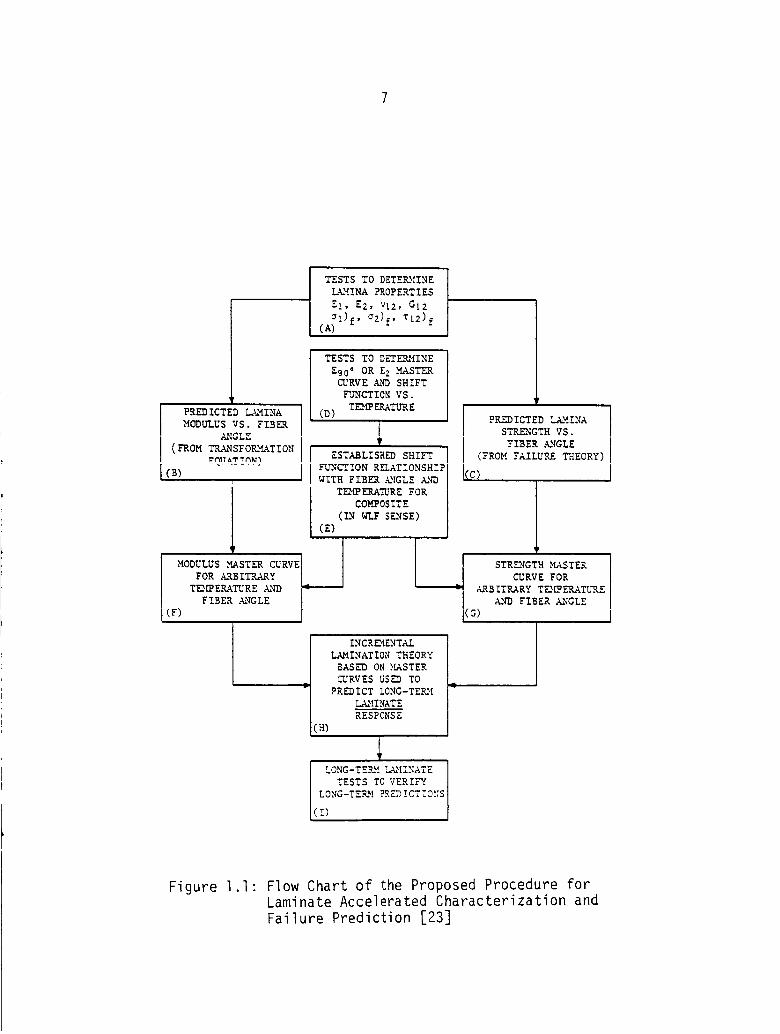
originally proposed is summarized in Figure I.I. The first
step in this proposed characterization process was to
determine the elastic constants of the unidirectional
composite lamina (EI,E2,GI2 , and _12 ) and the lamina failure
strengths (all , a2f ' and _12f) (A). The standard
transformation equations [24] were then used to obtain the
lamina modulii corresponding to any arbitrary fiber angle
(B), while a time independent failure theory was used to
obtain the failure strengths at these arbitrary fiber angles
(C). Creep tests were then performed to obtain the master
I PREDICTED L._INAMODULUS VS. FIB_
(FROM TRANSFORMATION
I(B) ..........
TESTS TO DETERMINELAMINA PROPERTIES
El, E2, vl2, Gl2
_l)f, _z)f, rl=)f(A)
TESTS TO DETEP_MINE
Ego° OR E2 MASTERCURVE AND SHIFTFUNCTION VS.TLMPERATURE
(D)
iT
I ESTABLISHED SHIFT
I FUNCTION RELATIONSHIPWITH FIBER ._TGLE AND
I TEMPERATURE FOR
COMPOSITE
(IN WI.FSENSE)(E)
T
MODULUS .MASTER CURVE I
FOR .A-RBITRARY I_ ITEmPeRATURE _NI)
FIBER ._GLE ]
(F) I
PREDICTED LA_!INA ISTRENGTH VS.
[ FIBER ._GLE 1(FROM FAILURE THEORY)
J
CURVE FORARBITRARY TD_ERATURE
(G) A_N'DFIBER ._NGLE I
iNCRSMENTAILAMINATION THEORYBASED ON }£ASTERCURVES USED TO
PREDICT LONG-TE_!LAMINATERESPONSE
!(H)
LONG-TERM LA_IINATETESTS TO VERIFY
LONG-TE_! ?RED!CT i0._:S
(l)
Figure l.l" Flow Chart of the Proposed Procedure forLaminate Accelerated Characterization andFailure Prediction [23]
8
curves and shift functions vs. temperature associated with
the TTSP (D). These results were used to establish the
functional relationship between fiber angle and shift
function (E). Once the shift function and modulii for any
arbitrary fiber angle were determined, a modulus master
curve for arbitrary temperature and fiber angle was
generated, again using TTSP (F). A strength master curve
was obtained for arbitrary temperature and fiber angle by
using the same shift functions obtained from the modulus
tests, with the implicit assumption that lamina strength
varied in a manner similar to the modulii (G). Finally, the
modulus and strength master curves at arbitrary temperature
and fiber angles were merged in incremental fashion using
CLT (H), which allows prediction of long-term laminate
response. The accuracy of the above analysis was checked by
actual long-term tests of a few selected composite laminates
(1).
A great deal of research involving the accelerated
characterization of composites has been performed since
1978. Extensive creep and creep rupture studies have been
conducted using the graphite-epoxy composite material system
T300/934. These tests were conducted at a variety of stress
levels ranging from a few hundred psi to ultimate strength
levels, and at a variety of temperatures ranging from room
temperature to temperatures near the glass transition

temperature (Tg) of the epoxy matrix. Creep tests for
0-deg, 90-deg and 10-deg off-axis T300/934 specimens have
been performed, as well as tests involving a variety of
symmetric laminate layups. Perhaps the most important
conclusions reached during these studies on T300/934 are:
* The fiber-dominated modulus E1 is essentially time-
independent [25]. Step (D) therefore requires creep
tests to obtain master curves for E2 and GI2 only.
* The principal compliance matrix used in the modulus
transformation equations remains symmetric even after
viscoelastic deformation with time [25]. Step (B) is
therefore valid.
* The shift function associated with the WLF equation 1
(step E) is independent of fiber angle [25]. This same
conclusion has also been reported elsewhere [26].
The assumption that lamina strength varies in a manner
similar to the modulii (step G) remains a reasonable but
unproven assumption for T300/934 graphite-epoxy. A major
difficulty encountered in assessing this concept has been
I. The WLF equation will be defined in Chapter II.
i0
the collection of consistent creep rupture data.
Considerable data have been collected, but excessive scatter
prevents any conclusive interpretations. However, evidence
supporting this assumption has been reported in reference
[27], where experimental data are presented indicating that
the fracture shift factors obtained for both a neat resin
matrix and a graphite-epoxy composite were nearly identical
to the compliance shift factors obtained using the same two
materials.
The overall conclusion reached during the VPI&SU studies
is that the accelerated characterization plan depicted in
Figure I.I can be used to provide reasonably accurate
predictions of long-term laminate response, at least for the
T300/934 material system studied.
During the course of these studies, it became desirable
to modify the proposed characterization plan by replacing
the TTSP with some other viscoelastic modeling technique,
for two reasons. First, Ferry reports [28] that the TTSP
was proposed by Leaderman in 1943 as an empirical curve-
fitting procedure. Since that time a theoretical basis for
the TTSP has been developed, but only for linear
viscoelastic behaviour, and only for temperatures at or
above the T of the material. Composites are used forg
structural applications at temperatures well below their Tg
to preserve structural rigidity. Additionally, nonlinear
ii
viscoelastic behaviour has been observed for composites,
particularily in shear [18,22,29]. Therefore, even though
the TTSP appears to provide reasonably accurate predictions
for composites, the use of the TTSP under the present
conditions is not rigorously justified. Secondly, the
conventional TTSP is a graphical procedure, requiring
horizontal and vertical shifts of the experimental data to
provide smooth uniform master curves. Producing these
master curves is a tedious, time-consuming process which is
subject to graphical error. Also. the amount _n_ type ef
vertical shifting required depends upon the specific
material system being studied, and no general rule exists
for all materials which might be considered [19]. Hence, the
TTSP is unwieldy when compared to other available
viscoelastic models which are readily adapted to computer
automation.
Two viscoelastic models were considered as replacements
for the TTSP. These models were the theory proposed by
Findley [30-32] and the theory proposed by Schapery [33-35].
The Findley theory is essentially empirical, whereas the
Schapery theory can be derived using the concepts of
irreversible thermodynamics. It has recently been pointed
out that the Schapery theory can be considered to be an
analytic form of the Time-Stress Superposition Principle
(TSSP) [22]. Both the Findley and Schapery theories are
12
relatively simple to apply and have been successfully used
to model a variety of materials. The model selected was
eventually determined by the available data base. That is,
the Findley theory requires only creep data to obtain the
various material parameters involved, whereas the Schapery
theory requires both creep and creep recovery data. Since
the existing data base contained only creep data, the
Findley theory was chosen to replace the TTSP, with the
recommendation that the Schapery theory be included in
future research endeavors.
An automated accelerated characterization scheme was
developed [21], and a computer program called VISLAP was
written which incorporates the accelerated characterization
scheme described above. The program provides long-term
predictions of the creep compliance and creep rupture times
for composite laminates of arbitrary layup. VISLAP was
modified for use during the present study, and details of
the program structure will be given in Chapter III.
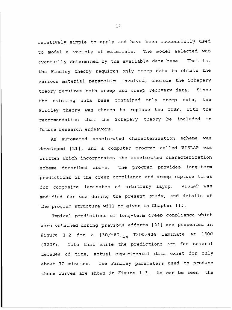
Typical predictions of long-term creep compliance which
were obtained during previous efforts [21] are presented in
Figure 1.2 for a [30/-60]_s T300/934 laminate at 160C
(320F). Note that while the predictions are for several
decades of time, actual experimental data exist for only
about 30 minutes. The Findley parameters used to produce
these curves are shown in Figure 1.3. As can be seen, the
13
(.__01 x)(ndt,_/1 ) 33NVlqd_O3 d_q,3_3
O. _ Q-- -- 0
( __01X ) (ISd/l) 33N?I-ldlAi03 dE_3

14
u-_IN3NO_XE M_'"i _3MOd
o o o
I
i = E
i 1340 ',\
(__01 x ) o__ -a..SNO_IS__ Sr'IO3N'_'..LN'_'.LS NI
o
00
I r f f ! _ I
v
I/)
1,1
F-
I"-'1o
I
0
i i
"Er_
_.. (.D
p.-
o
o-_
_g
g.
i,
(_.01 x) u_ _.LN31::)I__30:) /'A_'"I _3_Oe
15
instantaneous response, Zo' and the power law coefficient,
m, vary in a smooth and uniform manner. The power law
exponent, n, was expected to remain constant with stress but
experimental values show a significant scatter. An average
value for n was eventually used in the study. An analysis
of the power law showed that this instability was due to a
singularity in n [21]. The experimental data fell near this
singularity, and hence the evaluation of the power law
exponent was very sensitive to small errors in the
experimental data.
Predictions for creep rupture times are shown in Figure
I._, again for a [30/-6014 s T300/93_ laminate at 160C [21].
In general, the creep rupture data were characterized by
significant scatter, which was mainly attributed to
differences in the material properties of the composite
panels used in the study. A major contributor may have been
that the same postcure thermal treatment was not used for
all specimens, which would have caused considerable
differences in the viscoelastic response from specimen to
specimen. In most cases, the predicted rupture times were
conservative, although in some cases overly so.
Although the Schapery theory was not used in the
computer program VISLAP, it has since been successfully used
at VPI&SU to characterize the viscoelastic behaviour of
polycarbonate [36], bulk samples of FM-73 structural

16
(Dc:lW) SS3_.LS0 0 0 0 0
I l I l I
0
I I I_" oJ 0 cO
(!s_t) SS3_.LS
m
f'--1
I-,,,_1
C
',,.Ct,,-,-
0
0o,.Ic,")
I'_ e-,
0
W '
I
e-
W "O
o
t_
_D _-0 0 =
_J __
g
I '-"
°r I
I
17
adhesive [37], and unidirectional laminates of T300/93_
[22]. Since the Schapery theory is derived directly from
the principles of irreversible thermodynamics, it is
somewhat more appealing than the purely empirical Findley
equations. In addition, it accounts for some aspects of
nonlinear viscoelastic behaviour which the Findley equations
cannot model. Therefore, one of the objectives of the
present study was to integrate the Schapery theory with the
accelerated characterization scheme, and in particular to
insert the Schapery equations into the computer proqram
VISLAP.
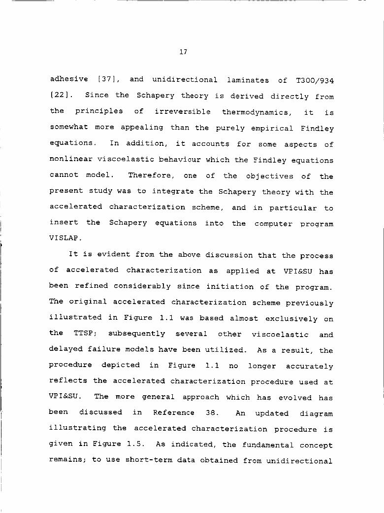
It is evident from the above discussion that the process
of accelerated characterization as applied at VPI&SU has
been refined considerably since initiation of the program.
The original accelerated characterization scheme previously
illustrated in Figure I.I was based almost exclusively on
the TTSP; subsequently several other viscoelastic and
delayed failure models have been utilized. As a result, the
procedure depicted in Figure i.I no longer accurately
reflects the accelerated characterization procedure used at
VPI&SU. The more general approach which has evolved has
been discussed in Reference 38. An updated diagram
illustrating the accelerated characterization procedure is
given in Figure 1.5. As indicated, the fundamental concept
remains; to use short-term data obtained from unidirectional
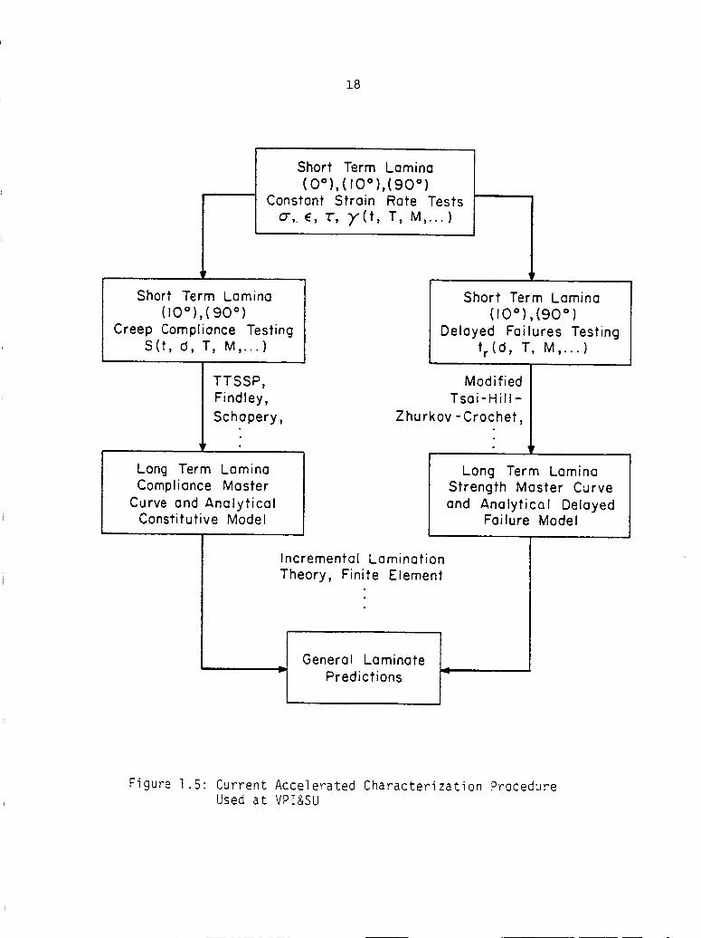
18
IShort Term Lamina
(_0°),(90 o)
Creep Compliance Testing
S(t, O, T, M,...)
Short Term Lamina
(0°),(10°),(90 °)Constant Strain Rate Tests
O-,.E, T, _'(t, T, M,...) lShort Term Lamina
(10°),(90 °)
Delayed Failures Testing
tr(d , T, M,...)
TTSSP,
Findley,
Schapery,
Long Term LaminaCompliance Master
Curve and AnalyticalConstitutive Model
Modified
Tsai-Hill-
Zhurkov-Crochet,
Long Term Lamina
Strength Master Curve
and Analytical DelayedFailure Model
Incremental Lamination
Theory, Finite Element
I General Laminate i= Predictions
Figure 1.5: Current Accelerated Characterization ProcedureUsed at VPI&SU
19
composite specimens to predict the long-term behaviour of
composite laminates of arbitrary layup.
Objectives of Present Study
The present
continuation of
described above.
research project is essentially a
the accelerated characterization study
It was felt that previous studies had
validated the concept of accelerated characterization, but a
further refinement of the technique in terms of a more
accurate compliance model and improved testing procedures
was required. In addition, previous efforts focused
exclusively on T300/934 graphite-epoxy. A different
material system was selected for use in the present study;
T300/5208 graphite-epoxy. This system was used because its
viscoelastic behaviour had not been studied previously at
VPI&SU. The intent was to validate the accelerated
characterization method by ascertaining if it would be
applicable to a new material system. Successful application
would serve to indicate whether the method could be
confidently applied to arbitrary reinforced plastics in
general as well as T300/934 in particular.
Based upon these general guidelines, the following six
program objectives were identified:
2O
(I) The integration of the Schapery nonlinear viscoelastic
theory with the accelerated characterization procedure.
This principally involved modification of the computer
program VISLAP, including additions and improvements to two
subroutines, called INPUT and VISCO, and the creation of a
new subroutine containing the Schapery equations, called
SCHAP.
(2) To perform a numerical study of the sensitivity of the
Findley/Schapery viscoelastic parameters to slight
experimental error in strain measurement. As indicated in
Figure 1.3, the experimentally determined values for the
power law exponent n have been subject to significant
scatter. Similar scatter has also been reported for the
Schapery parameters determined using similar experimental
procedures [37]. While a percentage of this scatter was
undoubtedly due to actual differences in mechanical
behaviour from specimen-to-specimen, there was some
indication that it was also in part due to a very high
sensitivity to experimental error which was accentuated by
the particular creep and/or creep recovery testing schedule
being employed.
(3) To develop a standard methodology in selecting a
creep and/or creep recovery testing schedule. This
methodology was to be based upon the results of objective
21
(2), and it was expected that the procedure developed would
be applicable to any viscoelastic material system, and not
just graphite-epoxy composites.
(4) To apply the accelerated characterization procedure
to the T300/5208 graphite-epoxy material system. The testing
program used was to be based upon the guidelines developed
as objective (3). Short-term creep and creep recovery tests
were to be performed on 90-deg and 10-deg off-axis
specimens, at an ambient temperature of 149C (300F). This
data would then be used with the Droqram VISLAP to Generate
long-term compliance predictions.
(5) To obtain long-term experimental measurement of the
creep compliance of two distinct T300/5208 laminates at 149C
(300F). In previous studies at VPI&SU, compliance
measurements were obtained for a maximum time of only 104
minutes (6.9 days). Therefore, it was felt that compliance
measurements at longer times were required to provide a more
rigorous check of predicted long-term behaviour. The two
distinct laminate layups were to be selected such that the
stress state applied to each layup and hence the
viscoelastic response would be significantly different for
each layup. Since there was no existing equipment available
for such a test, it was also required to design and
fabricate a multiple-station creep frame for this purpose.
22
(6) To compare the long-term experimental measurements
obtained as objective (5) with the long-term predictions
obtained as objective (4). The accuracy of the predictions
at very long times was of particular interest, as was
whether a conservative prediction of compliance at
relatively short times remained a conservative prediction at
very long times.
Background information related to the present study is
given in Chapter II, including brief reviews of viscoelastic
theory and classical lamination theory. The efforts to
achieve each of the above objectives are described in
Chapters III through VIII', followed by a summary and
conclusions discussion presented in Chapter IX.

II. BACKGROUND INFORMATION
The Theory of Viscoelasticity
Viscoelasticity is the study of materials whose
mechanical properties exhibit both a time-dependency and a
memory effect. For example, if a tensile specimen of a
viscoelastic material is subjected to a constant uniaxial
load, the specimen will "creep", and the apparent Young's
modulus will steadily decrease with time (or equivalently,
th_ apparent compliance of the material will steadily
increase with time). The viscoelastic material will
initially remain in a deformed state after unloading, but
will "remember" its original configuration and with time
will tend to "recover" back towards that configuration.
It is apparent from this definition that many time-
dependent phenomena are not necessarily viscoelastic. The
mechanical properties of an epoxy change with time during
the curing process, for example, but this time-dependency is
due to permanent microstructural changes in the molecular
chains of the epoxy. Once the cure is complete, there is no
tendency for the epoxy to return to its former state, and
hence there is no memory effect. Thus, for a phenomenon to
be considered viscoelastic, both time-dependency and memory
effects must be exhibited.
23
24
Three types of experimental tests commonly employed to
characterize viscoelastic materials might be considered for
use during the present study. These are the creep/creep
recovery test, the stress relaxation test, and the constant
strain rate test. The creep/creep recovery test is
illustrated in Figure 2.1. A uniaxial step load is applied
to the specimen, resulting in an axial stress which is held
constant for a time t I. If the test material is
viscoelastic, the specimen "creeps" for times in the range
of 0 < t < t I After time t I the load is removed and the
viscoelastic material "recovers" towards its initial
configuration.
Strain and stress histories for a stress relaxation test
are illustrated in Figure 2.2. In this test, a uniaxial
step deformation is applied to the specimen, resulting in an
axial strain which is held constant for the duration of the
test. The applied deformation induces an initial axial
stress _ which slowly "relaxes" with time.o
The constant strain rate test is illustrated in Figure
2.3. The specimen is subjected to an axial strain which is
increased at some constant rate R, and the axial stress
induced within the specimen is monitored. If the test
material is viscoelastic, the induced stress will not
increase linearly with time, as indicated.
In the present study, the creep/creep recovery test was
25
_=
C_
v I Time
_=
"T=
_0
t I Time
Figure 2.1: Stress and Strain Histories for a Creep/CreepRecovery Test
26
°r---
5..
o
Time
c_
Cz_
(T0
Time
Figure 2.2: Strain and Stress Histories for a Stress RelaxationTest

//
/
27
Tim
Figure 2"3: Strain and Stress
Rate Test Histories
T
for a Constant Strain
28
used almost exclusively to characterize viscoelastic
material behaviour, primarily because creep/creep recovery
tests are the easiest to perform. Constant strain rate tests
were used occasionally to obtain "instantaneous" modulii,
but were not used to obtain any viscoelastic parameters.
The stress relaxation test was not used in this study.
Viscoelastic materials are sometimes loosely grouped as
viscoelastic "solids" or viscoelastic "fluids". The
distinction between these two materi_l types is illustrated
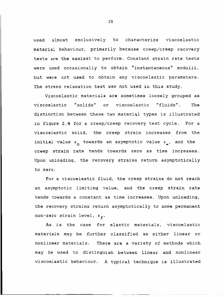
in Figure 2.4 for a creep/creep recovery test cycle. For a
viscoelastic solid, the creep strain increases from the
initial value _ towards an asymptotic value c , and theo
creep strain rate tends towards zero as time increases.
Upon unloading, the recovery strains return asymptotically
to zero.
For a viscoelastic fluid, the creep strains do not reach
an asymptotic limiting value, and the creep strain rate
tends towards a constant as time increases. Upon unloading,
the recovery strains return asymptotically to some permanent
non-zero strain level, Ef.
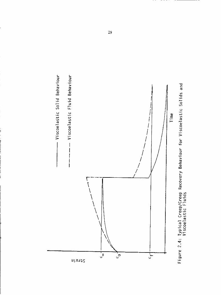
As is the case for elastic materials, viscoelastic
materials may be further classified as either linear or
nonlinear materials. There are a variety of methods which
may be used to distinguish between linear and nonlinear
viscoelastic behaviour. A typical technique is illustrated
29
i. i-
•"_ -x0 0
e- e-
°p .p-
Q
_ u°r...- °r..-
0 QU U
°P- °r.-
IIIII
\
u_e_s
\\\\\
8 obJ
I
////
//
/l /
(.,,.)
V)
0
(,_9
E
0U
°p,,.
i-0q..
i-
0
e"
S,-
O
eY
el m
I_l °r-
_ Q
.r'-'
3O
in Figure 2.5, where "isochronous" (i.e., constant time)
stress-strain curves are shown for both linear and nonlinear
materials. These curves would be generated using data
collected during several creep tests. Nonlinear behaviour
is readily identified using this technique, as shown.
The mathematical modeling of viscoelastic behaviour is
complicated considerably by nonlinear behaviour. As a
result, the theory of linear viscoelasticity is very well
developed and understood, while nonlinear viscoelasticity
theory has received attention only relatively recently and
is not as well developed nor understood.
In the present effort, the theory of viscoelasticity
will be used to characterize the epoxy matrix used in a
composite laminate. An important property which impacts the
viscoelastic behaviour of all polymeric materials is the
glass transition temperature (Tg). As the temperature of a
polymeric material is raised through the Tg, the elastic
modulus can decrease by a factor of 103 or greater. At
temperatures well below the Tg, polymers are generally very
brittle, exhibiting little or no viscoelastic response. At
temperatures above the Tg, polymers are extremely ductile
and "rubbery", exhibiting considerable viscoelastic
behaviour. This dramatic change in material behaviour
occurs over a narrow temperature range, on the order of 6C
(10F). For epoxies, the T is usually about 160C (320F).g
31
0°_
..C
t_Q
U*r-*
t_e--
0
00
.p-
c_
0t-
-J
0
e-
e_
U
0
U
.p-
°r,-
0
II
I
1I
A
ssa_S
c_-lJ
¢.)°_
0U
.f--
t__J
*p-
p--
c-
O
c-t_
.p-
.-S
c-.r--
p--
S..
4JO_!
_J
OO
0 _-
0 0_- .r--
c-O t_0 c-
d
t_
°_,.
32
The amount and type (i.e., linear or nonlinear, solid or
fluid) of viscoelastic behaviour which is exhibited by
polymeric materials is dependent upon a variety of factors,
including stress level, temperature, previous thermal
history, humidity, and molecular structure.
Linear Viscoelasticity.
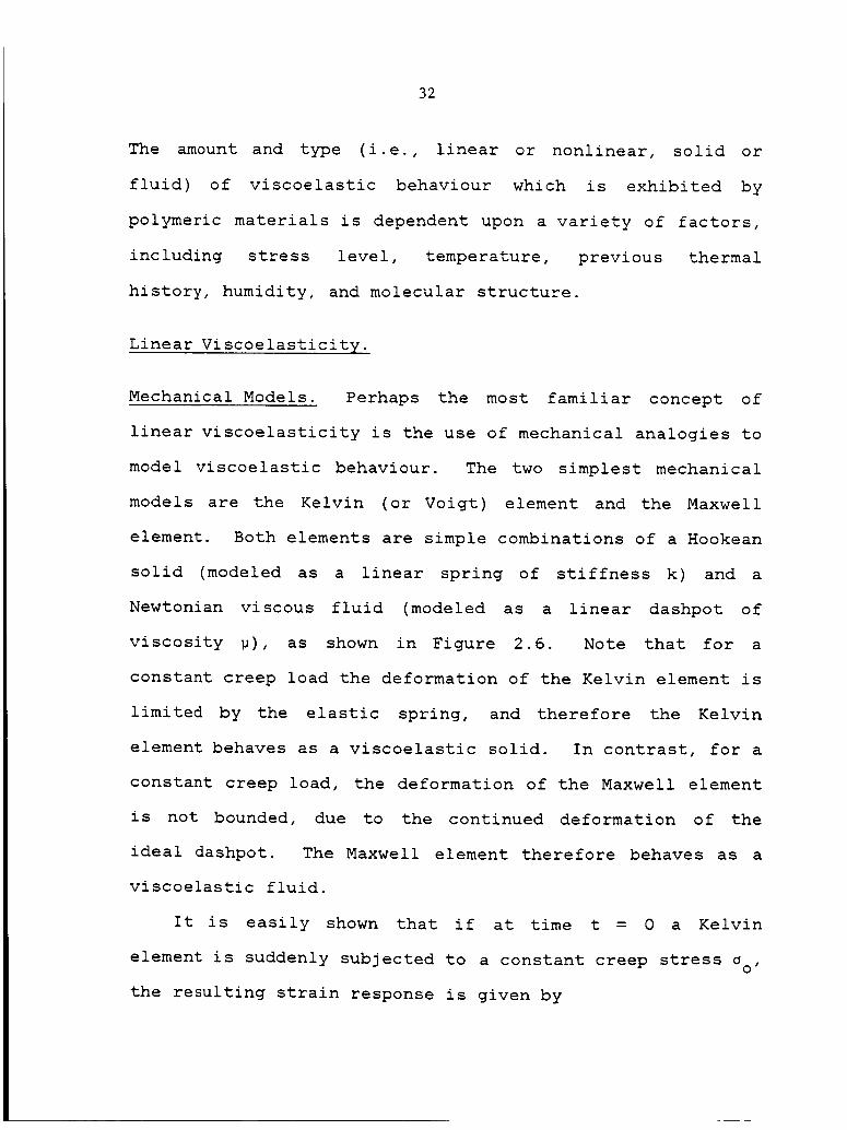
Mechanical Models. Perhaps the most familiar concept of
linear viscoelasticity is the use of mechanical analogies to
model viscoelastic behaviour. The two simplest mechanical
models are the Kelvin (or Voigt) element and the Maxwell
element. Both elements are simple combinations of a Hookean
solid (modeled as a linear spring of stiffness k) and a
Newtonian viscous fluid (modeled as a linear dashpot of
viscosity _), as shown in Figure 2.6. Note that for a
constant creep load the deformation of the Kelvin element is
limited by the elastic spring, and therefore the Kelvin
element behaves as a viscoelastic solid. In contrast, for a
constant creep load, the deformation of the Maxwell element
is not bounded, due to the continued deformation of the
ideal dashpot. The Maxwell element therefore behaves as a
viscoelastic fluid.
It is easily shown that if at time t = 0 a Kelvin
element is suddenly subjected to a constant creep stress _o'
the resulting strain response is given by

33
k
a) Kelvin Viscoelastic Element
k
b) Maxwell Viscoelastic Element
Figure 2.6: Simple Mechanical Analogies Used to ModelViscoelastic Behaviour
34
(_0 -t/T)=-V (i - e
where
- _ - the "retardation time"k
A typical viscoelastic response for a Kelvin element is
shown in Figure 2.7. Note that the retardation time _ is
determined by the viscosity and stiffness values selected
for the dashpot and spring, respectively.
In an analogous fashion, the stress within a Maxwell
element which is induced by a suddenly applied constant
strain ¢o is given by
a(t) = k e eo
where
-- _ -- the "relaxation time"k
Again, the relaxation time is defined by the viscosity and
stiffness values selected.
The behaviour of many viscoelastic materials cannot be
modeled by using a single Kelvin or Maxwell element, but can
be accurately modeled using the "generalized" Kelvin or
Maxwell models. The generalized Kelvin and Maxwell models,
shown in Figure 2.8, are composed of many (in some cases an

35
I
i
IIIIIIIIIIIII
0
0
_JE.r..-
0
0
O
0
c5
II
t)0 .._
II
h_
o_
E
c-
f,...
04_
¢1
c-O
°r.-
0
.t-
.r-e_
I'-"
°0
P_
M
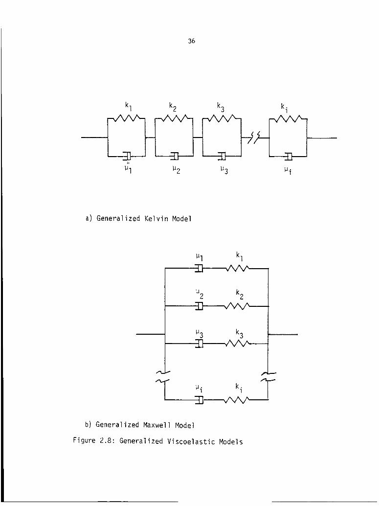
36
k I k 2 k 3 k i
Ii
Ul _2 _3 _i
a) Generalized Kelvin Model
Ul kl
U2 k2
u3 k3
T ui ki T
b) Generalized Maxwell Model
Figure 2.8" Generalized Viscoelastic Models

37
infinite number of) Kelvin or Maxwell elements, acting in
concert. For a generalized Kelvin model there is not a
single retardation time, but rather many retardation times
distributed over several decades in time. Furthermore, a
distinct contribution to compliance can be associated with
each retardation time. The distribution of these compliance
increments over time is called the retardation spectrum and
is usually written L(_), where L(_) has units of area/force.
In an analogous fashion, the generalized Maxwell model
possesses many relaxation times, and a distinct contribution
to stiffness can be associated with each relaxation time.
The distribution of these stiffness increments over time is
called the relaxation spectrum and is usually written H(_),
where H(_) has units of force/area. In principle, the
behaviour of any viscoelastic material can be modeled using
the generalized Kelvin or Maxwell models with an infinite
number of elements by simply imposing the appropriate
retardation or relaxation spectrums. A schematic
representation of a continuous retardation spectrum is shown
in Figure 2.9. There are also several molecular theories
which can be used to approximate the continuous viscoelastic
spectra with discrete spectrum lines [28,39], in which case
a finite number of Kelvin or Maxwell units is used. For
example, the creep response of a generalized Kelvin model
consisting of n Kelvin elements is given by

38
(_o_o)/_e_) (_)7
E
E.r.= _--_'- O
£.
%°r==
i--
q-
0
c-O
r_
t-
.w--
E
c--
(.,'3
d
£.
°r,-
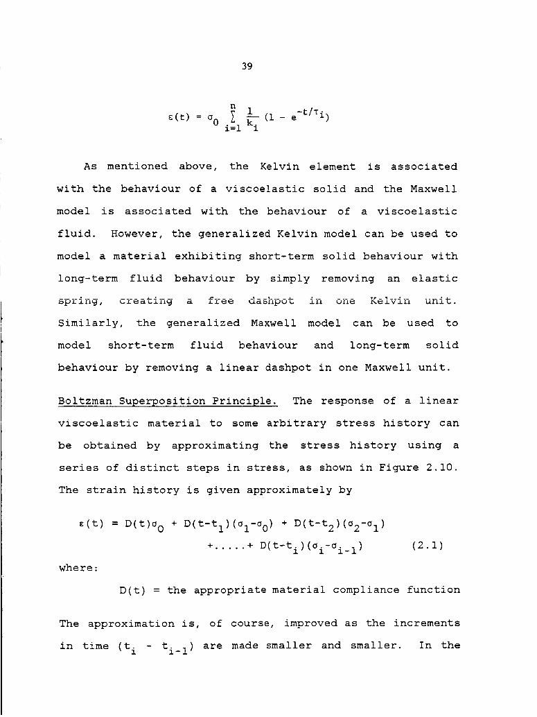
39
n
_(t) --_0 _ k7.1(i - e-t/Ti)i=l I
As mentioned above, the Kelvin element is associated
with the behaviour of a viscoelastic solid and the Maxwell
model is associated with the behaviour of a viscoelastic
fluid. However, the generalized Kelvin model can be used to
model a material exhibiting short-term solid behaviour with
long-term fluid behaviour by simply removing an elastic
_i_, creating = _== dashpot in one Kelvin unit.
Similarly, the generalized Maxwell model can be used to
model short-term fluid behaviour and long-term solid
behaviour by removing a linear dashpot in one Maxwell unit.
Boltzman Superposition Principle. The response of a linear
viscoelastic material to some arbitrary stress history can
be obtained by approximating the stress history using a
series of distinct steps in stress, as shown in Figure 2.10.
The strain history is given approximately by
z(t) = D(t)c 0 + D(t-tl)(Cl-C0) + D(t-t2)(c2-Cl)
+ ..... + D(t-ti)(ci-ci_l)
where:
(2.1)
D(t) = the appropriate material compliance function
The approximation is, of course, improved as the increments
in time (t i - ti_l) are made smaller and smaller. In the
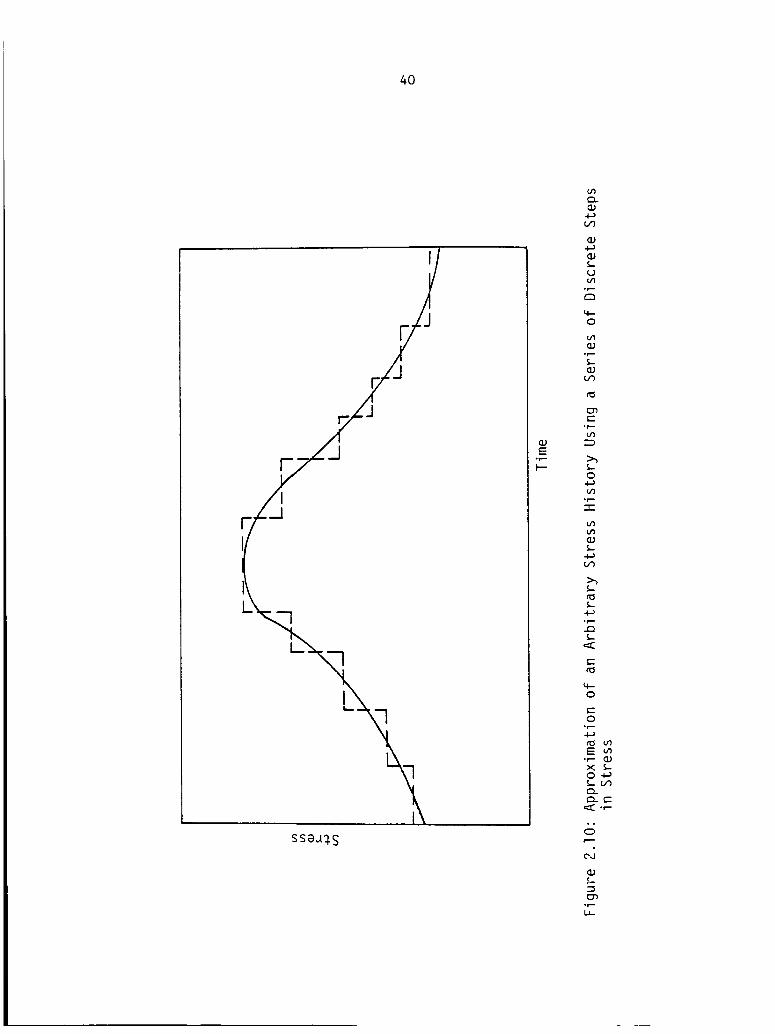
40
F, J
[-.
• :-I
L, ,--1
L
ssaa_s
Eor-
I---

41
limit eq. 2.1 becomes exact and may be written as
e(t) = D(t - T) da0- _- dT
(2.2)
Equation 2.2 is the well-known Boltzman Superpo sition
Principle, which gives the strain response for a linear
viscoelastic material to an arbitrary stress input. Note
that it has been assumed that the material has experienced
no previous stress or strain histories, i.e., o = _ = 0 for
--_ < t < O.
Time-Temperature Superposition Principle. As discussed in
Chapter I, the time-temperature superposition principle
(TTSP) was proposed by Leaderman in 1943 [28]. The TTSP is
also referred to as the "method of reduced variables" by
some researchers. This principle is of fundamental
importance to the present investigation because it is an
accelerated characterization procedure which has been
extensively studied and successfully used for a wide variety
of viscoelastic materials. The validity of the TTSP is
therefore firmly established, lending credibility to the
present efforts to characterize composite materials using an
accelerated characterization scheme.
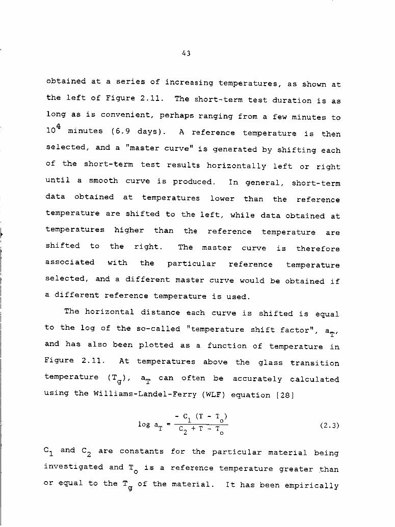
The steps in data reduction involved in the use of the
TTSP are summarized in Figure 2.11 for the case of stress
relaxation [40]. Short-term stress relaxation data are

42
o % o o o o £ o
UJOlseu£p(,_)_-qZ
o
i_..i
o
v_
ul
QJuoL
o-
¢:o
,_-.
oI..t_
o-
I--I--
..
I-..,-
O4
f...
I.l-
43
obtained at a series of increasing temperatures, as shown at
the left of Figure 2.11. The short-term test duration is as
long as is convenient, perhaps ranging from a few minutes to
104 minutes (6.9 days). A reference temperature is then
selected, and a "master curve" is generated by shifting each
of the short-term test results horizontally left or right
until a smooth curve is produced. In general, short-term
data obtained at temperatures lower than the reference
temperature are shifted to the left, while data obtained at
temperatures higher than the reference temperature are
shifted to the right. The master curve is therefore
associated with the particular reference temperature
selected, and a different master curve would be obtained if
a different reference temperature is used.
The horizontal distance each curve is shifted is equal
to the log of the so-called "temperature shift factor", a T ,
and has also been plotted as a function of temperature in
Figure 2.11. At temperatures above the glass transition
temperature (Tg), a T can often be accurately calculated
using the Williams-Landel-Ferry (WLF) equation [28]
- C 1 (T - T )o (2.3)
log a T = C 2 + T - T o
C 1 and C 2 are constants for the particular material being
investigated and T is a reference temperature greater thano
or equal to the T of the material. It has been empiricallyg
44
observed that for many polymeric materials the WLF equation
can be written
- 17.44 (T - T )$ (2.4)log aT = 51.6 + T - T
g
where in equation 2.4:
T > Tg
T, T in degrees Kelving
C1 = 17.44
C2 = 51.6
A material which can be characterized as described above
is referred to as a "thermorheologically simple material"
(TSM). For many materials a master curve cannot be formed
by means of simple horizontal shifting alone, however, and
some vertical shifting of the short-term data prior to
horizontal shifting is required. In these cases, the
material is referred to as a "thermorheologically complex
material" (TCM). Vertical shifting is often associated with
environmental effects such as temperature or humidity and
also with a nonlinear dependence on stress. Vertical and
horizontal shifting procedures have been extensively
reviewed by Griffith, et al [19], and will not be discussed
in greater detail here. It should be noted however that
vertical shifting introduces a significant complication in
the use of the TTSP, and is a major reason why alternate
45
accelerated characterization schemes have been pursued at
VPI&SU.
The Findley Power Law Equation. It has been empirically
observed that the creep compliance function for many
linearly viscoelastic polymeric materials can be accurately
modeled using a power law of the form
where
D(t) = A + Btn
A, B, n = material constants
t = time after creep loading
(2.5)
For a creep test, the stress history may be expressed as
where
c = co H(t), and therefore
dc- c 6(t)
dt o (2.6)
c = constanto
H(t) = the Heaviside unit step
_0, t < 0function
, t > 0
dH(t) _6(t) -
dtthe Kronecker-Delta
_, t = 0function
O, t#O
Substituting equations 2.5 and 2.6 into equation 2.2 results
in the so-called "Findley power law equation":
46
wher e
E(t) = _O + mtn
¢ =A co o
m= B co
Note from these definitions
considered material constants.
(2.7)
that ¢ and m are alsoo
Equation 2.7 has been used by Findley and his co-workers
to successfully characterize the viscoelastic behaviour of a
variety of amorphous, crystalline, and crosslinked polymers.
As presented here, it is valid only for linearly
viscoelastic behaviour. However, Findley has presented a
slightly modified form of eq. 2.7 for use with nonlinear
viscoelastic materials. This nonlinear Findley power law
will be described in the next section.
Nonlinear Viscoelasticity
Mechanical Models. It is theoretically possible to modify
the linear generalized Kelvin or Maxwell models to account
for nonlinear viscoelastic behaviour through the use of
nonlinear springs and/or dashpots. Since the retardation
(relaxation) times _. for the Kelvin (Maxwell) model are1
equal to the ratio _i/ki, this implies that _i is not a
constant for each Kelvin (Maxwell) element but rather a

47
function of stress level. Alternatively, nonlinear behaviour
can be introduced through the use of nonlinearizing
functions of stress as follows
where
n
iI 1 1 e-t/Ti)e(t) = _0 _ (i - fi(OO)
fi(CO) = nonlinearizing functions of stress
Hiel et al report [22] that Bach has used this approach to
model the nonlinear viscoelastic behaviour of wood.
Generalized mechanical models are rather cumbersome even in
the linear case however, and have not been used to model
nonlinear behaviour to any great extent.
Multiple-Integral Approaches. The viscoelastic constitutive
equation relating the strain and stress tensors can be
written in the most general form as
eij(t) = Fijkl [Okl(T)]
T=O
where
zij(t), Ckl(_) = strain and stress tensors,
respectively
Fijkl = continuous nonlinear compliance tensor
t = present time
= arbitrary time
(2 .S)

48
Equation 2.8 implies that the current strain state is
dependent upon the entire previous stress history, i.e.,
from 0 < _ < t. Thus, a material which can be described by
eq. 2.8 exhibits a memory effect and is viscoelastic.
In a series of publications [41-43], Green, Rivlin, and
Spencer presented an analysis which shows that eq. 2.8 can
be approximated to any degree of accuracy by a series of
multiple-integrals. This approach involves the use of
convoluted integrals containing n-th order terms of stress.
The final multiple-integral expression for three-dimensional
stress states is quite lengthy and will not be presented
here. A simpler expression derived by Onaran and Findley
[44] will be used to illustrate the fundamental concept.
Their expression is applicable for a uniaxial stress, and
only two orders of stress are retained. Using this approach
the following relation is obtained
z(t) = (t-_) a(_) d_ +
I t I t _2(t__,t_m) [c(%) ]2 dmd% +0 0
2 (t-_l,t-_2)O(_l)C(_2) d_ld_ 2 (2.9)0
The functions _1 and _2 which appear in eq. 2.9 are called
kernel functions and must be determined experimentally. If
a third order of stress were used in the derivation of eq.
2.9, a triple integral would appear involving a third kernel
49
function _3" Therefore, the number of tests required to
characterize a viscoelastic material using this technique
depends upon both the type of loading and the desired degree
of accuracy. If a general three-dimensional stress state
were assumed and only the first, second, and third orders of
stress terms are retained, there are still thirteen
independent kernel functions which must be evaluated. This
requires over I00 tests involving various combinations of
uniaxial, biaxial, and triaxial loading conditions. Such
extensive and difficult testing is impractical in most
instances. The multiple-integral approach has therefore not
been used to any extent in practice, even though it is
probably one of the most accurate and versatile nonlinear
viscoelastic theories available.
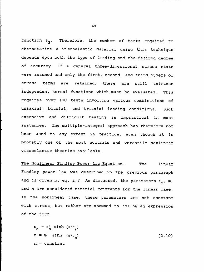
The Nonlinear Findley Power Law Equation. The linear
Findley power law was described in the previous paragraph
and is given by eq. 2.7. As discussed, the parameters _o' m,
and n are considered material constants for the linear case.
In the nonlinear case, these parameters are not constant
with stress, but rather are assumed to follow an expression
of the form
= ' sinh (alaE)E 0 E 0
m = m' sinh (a/am)
n = constant
(2.10)
50
where
¢' o m' o = material constantso' ' ' m
By substituting eqs. 2.10 into eq. 2.7 the nonlinear Findley
power law equation is obtained
!
e(t) = e sinh (o/_ e) + m't n sinh (o/_) (2. ii)O m
In eq. 2.11 the nonlinear dependence upon stress is assumed
to follow a hyperbolic sine variation in stress. Apparently
this assumption was originally based upon empirical
observation, although theoretical justification has since
been suggested [21,34,39]. This approach has been used
successfully by Findley and his coworkers to characterize
the viscoelastic response of many materials, including
canvas, paper, and asbestos laminates [30,31],
polyvinylchloride [32,44,45], and polyethylene,
monochlorotriflouroethylene, and polystyrene [45].
Equation 2.11 was developed for the case of constant
uniaxial creep loadings. Findley has also extended this
concept to account for nonlinear viscoelastic response to a
varying uniaxial load. This technique is called the Modified
Superposition Principle (MSP), and has been applied by
Findley et al to many of the materials mentioned above
[30,32,45]. More recently, MSP has been applied by Dillard
et al to characterize T300/934 graphite/epoxy laminates
[21], and by Yen to characterize SMC-R50 sheet molding
51
compound [46].
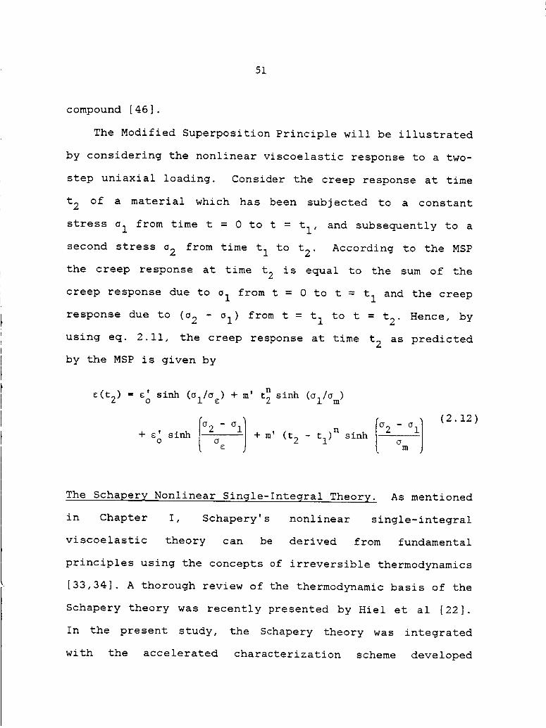
The Modified Superposition Principle will be illustrated
by considering the nonlinear viscoelastic response to a two-
step uniaxial loading. Consider the creep response at time
t 2 of a material which has been subjected to a constant
stress a I from time t = 0 to t = tl, and subsequently to a
second stress a2 from time t I to t 2. According to the MSP
the creep response at time t2 is equal to the sum of the
creep response due to o I from t = 0 to t = t I and the creep
response due to (_2 - al) from t = t I to t = t 2. Hence, by
using eq. 2.11, the creep response at time t 2 as predicted
by the MSP is given by
e(t 2) = e'o sinh (OllOe) + m' t2 sinh (Ol/Om)
+ e' sinho i 2-l-m,sinhi_i _ n _2 - _i]
(2.12)
The Schapery Nonlinear Single-Integral Theory. As mentioned
in Chapter I, Schapery's nonlinear single-integral
viscoelastic theory can be derived from fundamental
principles using the concepts of irreversible thermodynamics
[33,34]. A thorough review of the thermodynamic basis of the
Schapery theory was recently presented by Hiel et al [22].
In the present study, the Schapery theory was integrated
with the accelerated characterization scheme developed
52
during previous research "efforts at VPI&SU [21]. A detailed
description of the Schapery equations and the application of
these equations during the present study will be presented
in Chapter III, so further discussion of the Schapery theory
will be delayed until that point.
Classical Lamination Theory
A composite "lamina" or "ply" is a single membrane of
composite material in which strong and stiff, continuous
(i.e., very long) fibers have been embedded within a
relatively weak and flexible "matrix" material. All fibers
are aligned in the same direction, and the matrix serves to
bind the individual fibers together to form a single unit.
For polymer-matrix composites, laminae thicknesses are
usually on the order of 0.13 mm (0.005 inch). A composite
"laminate" is the bonded assemblage of several layers of
composite laminae. The number of laminae or plies within a
laminate can vary from a very few (say 4 or 5) to very many
(say 150), depending upon application.
Since all fibers within a lamina are orientated in the
same direction, a lamina is highly orthotropic and exhibits
very high strength and stiffness properties parallel to the
fibers and very low strength and stiffness properties
perpendicular to the fiber direction. A composite laminate
53
is therefore normally designed so that fiber orientation
relative to some reference direction varies from ply-to-ply,
providing good overall strength and stiffness
characteristics in more than one direction. An eight-ply
composite laminate is shown schematically in Figure 2.12.
This laminate is described as a [0/9012s laminate, meaning
that the O-deg/90-deg lamina pairs are repeated twice and
symmetrically about the middle surface of the laminate.
Note that the individual ply directions are referenced to
the x-axis.
Since a composite laminate may consist of any number of
plies, and each ply may be orientated in a different
direction, some method of predicting the overall elastic
mechanical properties of the laminate based upon the
properties of a single ply is required. Such a method has
been developed and is known as "classical lamination theory"
(CLT). The principal assumptions made in CLT are the plane-
stress assumption and the Kirchoff hypothesis, i.e., a line
which is initially straight and normal to the laminate
middle surface is assumed to remain straight and normal to
the middle surface after deformation. In addition, no out-
of-plane extensional strains are considered. A brief review
of the conventional equations used in CLT will be given
below. Notation will follow that of Jones [24].
A composite lamina is shown schematically in Figure

54
N
<
\
X
vl
11
t__m
ormEr_
mJ
C_4-)
O
O_J
0
0i l
04--
0
4-)_S
c_°r,-
0
c_r--
c_
_J_b
ottoil

55
<Y
\X
k\\\\\\\1k\\\L\\\_
\\\\\\\\
\
\f
/
Figure 2.13: Coordinate Systems Used to Describe a CompositeLamina

56
2.13. The coordinate systems used to describe the lamina are
the principal material coordinate system, axes 1 and 2, and
the reference coordinate system, axes x and y. The 1,2
coordinate system is rotated an angle 8 away from the x,y
system. Under plane-stress conditions the stress-strain
relations in the 1,2 coordinate system are given by the
orthotropic form of Hooke's law
°i _ QII QI2 o
°2 = L QI2 Q22 0r12 0 0 Q66
111s2
YI2
(2.13)
where
Qij = the "reduced stiffness matrix"
E 1 E 2
QII = i - _12 _21 Q22 = i - _12 v21
v12 E2 v21 E1
Q12 = Q21 = 1 - u12_21 1 - u12 v21
Q66 = GI2
In the x,y coordinate system, the stress-strain relations
are given by
III°x QII
Oy = QI2
Txy QI6
QI2 QI6
Q22 626
626 666
EX
ey
Yxy
(2.14)
where
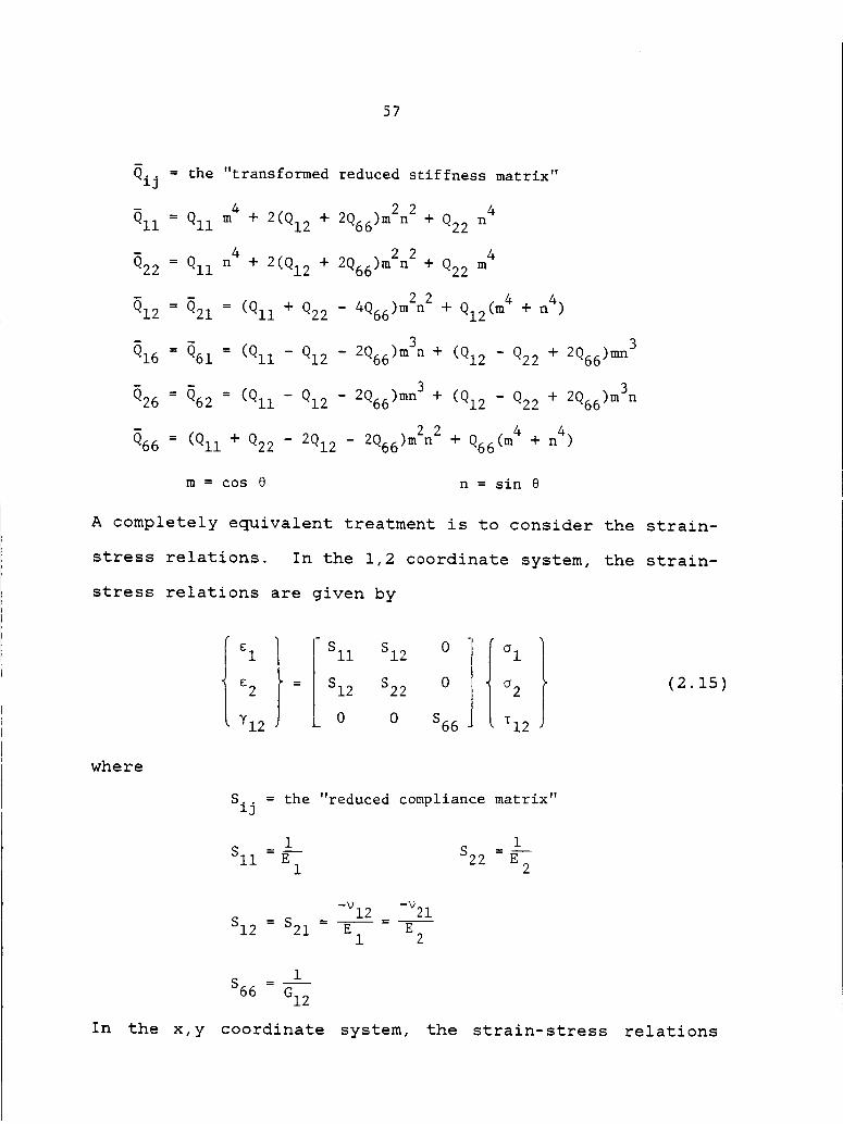
57
Qij = the "transformed reduced stiffness matrix"
m4 4QII = QII + 2(Q12 + 2Q66)m2n2+ Q22n
- n4 4Q22 = QII + 2(Q12 + 2Q66)m2n2+ Q22m
QI2 = Q21 = (QII + Q22 - 4Q66)m2n2+ QI2(m4 + n4)
QI6 = Q61 = (QII - QI2 - 2Q66)m3n+ (QI2 - Q22+ 2Q66)mn3
Q26 = Q62 = (Qll - Q12 - 2Q66)mn3+ (QI2 - Q22+ 2Q66)mBn
Q66 = (QII + Q22- 2Q12 - 2Q66)m2n2+ Q66(m4 + n4)
m = cos 8 n = sin 8
A completely equivalent treatment is to consider the strain-
stress relations. In the 1,2 coordinate system, the strain-
stress relations are given by
e1
a2
YI2i Sll S12 0
= S12 $22 0
0 0 $66[°l}o 2
_12
(2.15)
where
S.. = the "reduced compliance matrix"13
i iSII = _--- $22 = _--
1 2
-v12 -v21
S12 = $21 = --_--- =1 2
i
$66 = GI 2
In the x,y coordinate system, the strain-stress relations
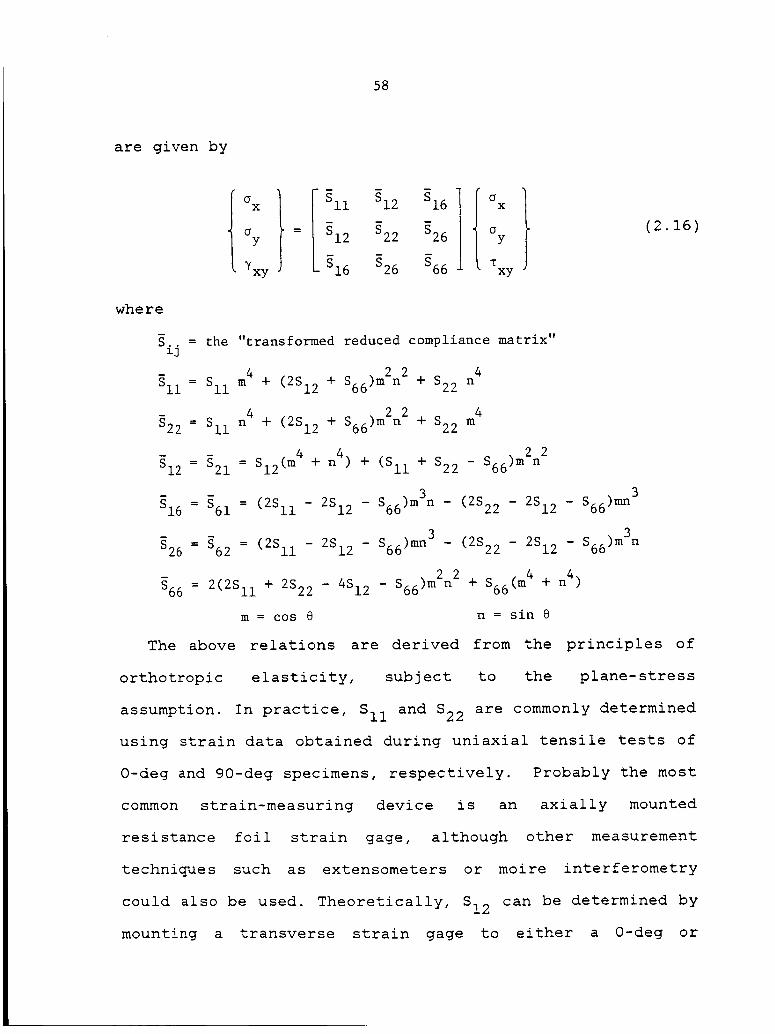
58
are given by
x 1 [ SIIay = I s12Yxy L s16
S12
22
S26
16
S26
$66I _x
ay
Txy
(2.16)
where
S.. = the "transformed reduced compliance matrix"zj
S66)m2n 2 4- = m4 + + + nSll SII (2S12 $22
S66)m2n 2 4n4 + + + m$22 = SII (2S12 $22
S12 = $21 = S12 (m4 + n4) + (SII + $22 - S66)m2n2
3
S16 = $61 = (2SII - 2S12 - S66)m3n - (2S22 - 2S12 - S66)mn
$26 = S62 (2Si I 2S12 S66)mn 3 - n- = - _ - (2S22 2S12 - S66)m 3
$66 = 2(2SII + 2S22 - 4S12 - S66)m2n2 + s66(m4 + n4)
m = cos e n = sin 8
The above relations are derived from the principles of
orthotropic elasticity, subject to the plane-stress
assumption. In practice, SII and $22 are commonly determined
using strain data obtained during uniaxial tensile tests of
O-deg and 90-deg specimens, respectively. Probably the most
common strain-measuring device is an axially mounted
resistance foil strain gage, although other measurement
techniques such as extensometers or moire interferometry
could also be used. Theoretically, S12 can be determined by
mounting a transverse strain gage to either a 0-deg or
59
90-deg specimen. However, the value of _21 is normally in a
range of about 0.01 to 0.05, and consequently the strains
measured using a transverse gage mounted to a 90-deg
specimen are very low. This can lead to relatively high
experimental error. In practice, it is preferable to
determine S12 using a transverse gage mounted on a 0-deg
specimen.
A variety of techniques have been proposed to determine
S66, including the rail-shear tests, picture-frame specimen
tests, and off-axis tensile snecimen t_sts. Tn n_tic1_]_
the 10-deg off-axis tensile test has been proposed by Chamis
and Sinclair [47] as a standard test specimen for
intralaminar shear characterization. Several proposed shear
characterization techniques were reviewed by Yeow and
Brinson [48], and it was concluded that of those methods
reviewed the 10-deg off-axis test was best suited for use,
primarily because it is inexpensive and easily performed,
while still providing an accurate measure of the shear
compliance. This technique was used during the present
study. Additional details of the 10-deg off-axis test will
be presented in Chapter VI.
The mechanical response of a composite lamina to in-
plane external loadings can be described as presented above.
The mechanical response of a composite laminate to external
loading can be described through the use of CLT, in
60
conjunction with the orthotropic elasticity relations
embodied in eqs. 2.13-16. Some results of CLT pertinent to
the present study will now be presented; readers desiring a
more detailed treatment are referred to the text by Jones
[24].
The resultant forces N. and resultant moments M. acting1 1
along the edges of a composite laminate can be expressed in
oterms of the middle surface strains E. and curvatures _.
3 3
as follows
{Ni} Aij1_7=I---_....-I.... (2.17)
where
t/2N. = o. dz
i J-t/2 l
t/2M. = o. z dz
z _-t/2 i
n
Aij = _ (Qij)k (Zk - Zk-l)k=l
i n 2 2
Bij = _ _ (Qij)k (zk - Zk_ I)k=l
I n (z 3 3Dij = 3 _ (Qij)k k - z _i )k=l
oe. = normal and shear strains induced at laminate middle surface3
K. = surface curvatures induced at middle surfaceJ
61
The z-direction is defined in a direction normal to the
middle surface. Hence, the quantity (z k - Zk_l) equals the
thickness of the kth ply within the laminate. The resultant
forces Ni are defined as the force per unit length acting
along the edge of the laminate. Similarly, the resultant
moments Mi are defined as the moment per unit length acting
along the edge of the laminate. The strain state of any ply
within the laminate can be expressed in terms of the middle
surface strains o and curvatures _. [24]] 3
Through inspection of eq. 2.17, it can be seen that a
coupling exists between the in-plane forces N. and the out-1
of-plane curvatures _j, due to the Bij matrix. Similarly, a
coupling exists between the out-of-plane bending moments M.1
O
and the in-plane middle surface strains _j, again due to
the Bij matrix. Such coupling is a major difference between
the behaviour of composite materials and more conventional
isotropic materials, since such coupling between in-plane
and out-of-plane forces and deformations does not occur for
isotropic materials. It can be shown that if a composite
laminate is "symmetric", such as the laminate shown in
Figure 2.12, then all elements of the B.. matrix are zero,13
and no coupling between in-plane and out-of-plane forces and
deformations occurs. During the present study, only
symmetric laminates were considered. In addition, the only
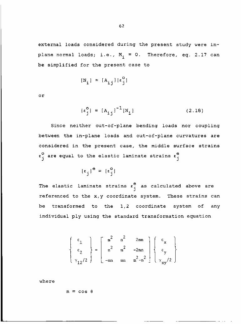
62
external loads considered during the present study were in-
. ., = 0 Therefore, eq 2.17 canplane normal loads; i e Mi .
be simplified for the present case to
{Ni} = [Aij ]{E_}3
or
{ o -Ij} = [Aij] {Ni} (2.18)
Since neither out-of-plane bending loads nor coupling
between the in-plane loads and out-of-plane curvatures are
considered in the present case, the middle surface strainso e
_. are equal to the elastic laminate strains _.3 ]
{_j}e = {oj}
The elastic laminate strains e. as calculated above are]
referenced to the x,y coordinate system. These strains can
be transformed to the 1,2 coordinate system of any
individual ply using the standard transformation equation
{liIm222 n2mn22ran2o22!I1xyY12/2 -mn mn m -n Yxy/2
where
m = cos 8
63
n = sin e
The elastic stresses acting within the kth ply,
referenced to the 1,2 coordinate system, can be calculated
using eq. 2.13
{0i}k ]k e1,2 = [QI2 {_j}1,2
The elastic strains are considered to be the difference
between the total laminate strains ct. and any residualJ
{zj}e = t r1,2 {¢j}1,2 - {cj}1,2
In the present case, the residual strains considered will be
those due to viscoelastic creep. Residual strains can also
be caused by thermal expansion or water absorption
(hygroscopic strains).
Finally, it should be noted that the above relations are
contingent upon the underlying assumptions of CLT, namely
the plane-stress assumption and the Kirchoff hypothesis.
Accordingly, this analysis is not valid for very thick
laminates or for regions near a free-edge. In both of these
latter cases, a three-dimensional stress state is induced,
including interlaminar shear stresses [1-3].
III. THE SCHAPERY NONLINEAR VISCOELASTIC THEORY
One of the objectives of this study was to integrate the
Schapery nonlinear viscoelastic model with the accelerated
characterization scheme previously developed at VPI&SU.
This principally involved the inclusion of the Schapery
equations in an existing computer program called VISLAP,
written by Dillard [21]. The efforts to attain this
objective will be described in this chapter. In the
following section, the Schapery model will be reviewed, and
the methods used to incorporate the appropriate equations
into the present analysis will be described. This
discussion is followed by a section describing the program
VISLAP, as modified for use during the present study.
It should be noted that VISLAP is capable of predicting
both the long-term creep response and creep rupture times of
symmetric composite laminates. In the present study, creep
rupture was not considered, and so in the following
discussion creep rupture will be mentioned only to provide
an overall review of the VISLAP program.
The Schapery Viscoelastic Model
As mentioned in Chapter I, the Schapery nonlinear
viscoelastic theory can be derived from fundamental
principles using the concepts of irreversible thermodynamics
64
65
[33,34], and a comprehensive review of the thermodynamic
basis of the Schapery theory has recently been presented by
Hiel et al [22]. The theory has been successfully applied
to a variety of materials, including glass fiber-epoxy
composites [35], T300/934 graphite-epoxy composites [22],
nitrocellulose film, fiber-reinforced phenolic resin, and
polyisobutylene [49], and FM-73 structural adhesives
[37,50,51].
For the case of uniaxial loading at constant
temperature, the Schapery theory reduces to the following
single-integral expression
t dg2oc(t) = go AoO + gl 0- AA(_-_') _ dT
where
(3.1)
Ao' AA(¢) = initial and transient components of the
linear viscoelastic creep compliance,
respectively
t= ¢(t) = dt
0- ao
T dt= (t) = --0- ao
go' gl' g2' ao = stress-dependent nonlinearizing
material parameters

66
Several points should be noted regarding eq. 3.1.
the initial
compliance, Aostress level.
First,
and transient components of the creep
and AA(_), are assumed to be independent of
That is, at a given temperature both A andO
AA(#) are assumed constant for any stress level, and all
nonlinear behaviour is introduced through the four stress-
dependent nonlinearizing parameters go' gl' g2' and a c-
Secondly, no assumption is implied regarding the form of Ao
and AA(#), and theoretically any form suitable for use with
the material being investigated may be used. It is often
assumed that AA(_) can be approximated by a power law in
time (as will be discussed below), but this is not an
implicit assumption within the Schapery theory. Thirdly, if
the material is linearly viscoelastic, then go = gl = g2 =
a = 1 and eq. 3.1 reduces to the familiar Boltzmanc
Superposition Principle (eq. 2.2). Finally, the effect of
the stress-dependent parameter a c , embedded within the
expressions defining the "reduced time" parameters _ and
_', is to "shift" the viscoelastic time scale, depending
upon stress level. The a parameter can therefore beO
considered to be a "stress shift factor", analogous to the
familiar "temperature shift factor", a T , used in the TTSP
and discussed in Chapter II. In this light the Schapery
theory can be considered to be an analytical form of a Time-
Stress Superposition Principle (TSSP).

67
If closed-form expressions for go' gl' g2' and ac as
functions of stress are available, and if the form of A andO
AA(_) are known, then it is theoretically possible to
integrate eq. 3.1 and obtain an expression for the
viscoelastic response _(t) for any uniaxial stress history
c(t). In general such closed-form expressions are not
available however, and subsequently simple stress histories
must be assumed in order to integrate eq. 3.1. However,
during the present study a procedure was developed whereby
the viscoelastic response to a complex uniaxial stress
history can be approximated to any desired degree of
accuracy by using a series of discrete steps in stress.
This approach will be described below and is similar in
concept to the Modified Superposition Principle proposed by
Findley and his colleagues, which was discussed in Chapter
II.
The first step in the application of the Schapery theory
is to establish an analytic form of the transient component
of the creep compliance, AA(_), which is suitable for use
with the material being investigated. In previous
applications of the Schapery theory, AA(_) has been modeled
using a power law approximation of the form
AA(_) = C_ n (3.2)
This form was also used in the present study. In eq. 3.2
68
both C and n are assumed to be material constants at any
stress level, for a constant temperature. Substituting eq.
3.2 into eq. 3.1 results in
t )n dg2 os(t) = go A a + gl C (_-_' -- dTo 0- dY
(3.3)
Now consider the stress history applied during a creep/creep
recovery test cycle, as previously illustrated in Figure
2.1. This stress history can be expressed mathematically as
o(t) = Oo[H(_) - H(_ - tl)]
and therefore
dg 2 o
dT = g2 °0 [6(_) - _(r - tl)]
For times 0 < t < t I,
therefore
the stress is a constant, c = c o , and
dg 2 c
dT = g2 °0 6(_)
t dt _ t@ = - a a0 o o
=0_' = d-it= 0
0- ao
Substituting these relations into eq. 3.3 results in
69
Ig glg 2 C tn]ec (t) = 0A + n a0
o a
(3
Equation 3.4 is the Schapery equation for creep, and is
applicable for times 0 < t < tI. The values of go' gl' g2'
and a are dependent upon the applied creep load go" The
instantaneous response at time t = 0 will be of interest in
_^ fol I...._ di " _ _ _ A +_ _=_ _ _im_
t = O iS calcu±atea as
A¢(0) = g0AoC0
Now consider the recovery strains during times t > t I.
The current applied stress is now _ = 0, and hence go = gl =
I, and eq. 3.3 becomes
t dg2aer(t) = C (___,)n __ aT (3 5)0- dT
Since the stress history _(t) is discontinuous, eq. 3.5 must
be broken into two parts
- dg2____a° I t )n dg2°er(t) = C tl (___,)n dr + C (_-_' dr
0- dT tl
dT (3.6)
70
for I tl :0- dg2o
d---_= g2oO_(_)
- ItitdtI td +__= aO- ao o t I
_' = I_=0 dta0 o
-0
dt tl---+t- t I
i a
tfor
tI____.__..-.---------
dg2° 6(__tl )d--?-= - g2°O
t dt tl-_+t- tI@ = a
O- ao o
I_=tl dt tl_'= %--= a-_
:0- o
Substituting the above relations into eq. 3.6 results in
gr (t) = g2 C a 0 _ tI j
(3.7)
The following quantities are next defined
t I
O
t - t I
tI
II
4g I = glg 2 C _i °o
71
and equation 3.7 is rewritten in a simpler form as
A_I
r gl[(i + aoX)n - (aox)n] (3.8)
In the
equation in the form of eq. 3.8.
An interesting consequence of
involves the instantaneous change
literature, Schapery has presented the recovery
the
in
Schapery theory
strain following
If the recoveryremoval of the creep load at time t I.
strain predicted immediately after t I (calculated using eq.
3.8) is subtracted from the creep strain predicted
immediately before t I (calculated using eq. 3._), the
following expression is obtained
n
C t1
Ae(tl) = g0Ao°0 + (gl - l)g2 n °0aO
The instantaneous response to the creep load has already
been shown to be
AE(O) = goAoOo
Thus, the instantaneous change in strain following removal
of the creep load at time t I equals the instantaneous
72
response at time t = 0 only if the material is linear, i.e.,
if gl = 1.0. If gl > 1.0, then AE(tl) > _(0), and the
resulting nonlinear recovery curve is "flatter" than the
corresponding linear recovery curve. If gl < 1.0, then
A_(tl) < At(O) and the nonlinear recovery curve is "steeper"
than the linear recovery response.
The viscoelastic response to the two-step loading
illustrated in Figure 3.1 can be derived using similar
mathematical procedures [49]. For example, for times t >
t I, the viscoelastic response is given by
2 2 [glol_n + (g2202_gl(_l)[_ _ _] n]e(t) = g0Ao°2 + gl C 2 (3.9)
where
tI t - t1
=-Y+ 2a a0 o
In eq. 3.9, the superscripts associated with each of the
nonlinearizing parameters denote the stress level at which
these parameters are to be evaluated. For example, g_
indicates that g2 is to be evaluated at stress 02 .
During the present study, the Schapery theory was to be
used to predict the viscoelastic response of individual
plies within a composite laminate. In previous efforts, the
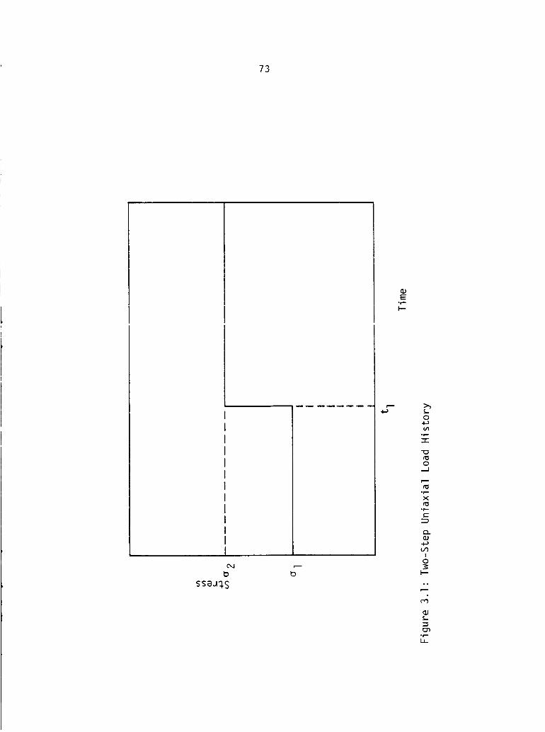
73
Eo1---
I---
,-- >_
o
.I'm
--T-
O.J
%°1_
x
Q.
(._!
ss_J_Sb
O
o°
p--
E_°I--
i,
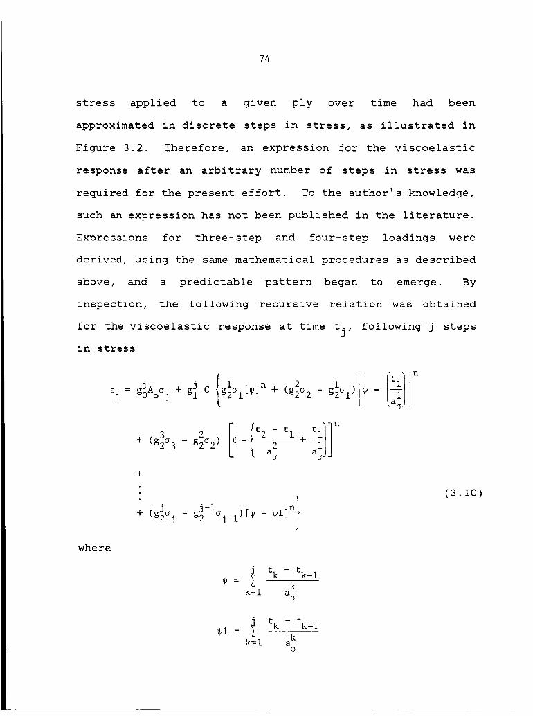
74
stress applied to a given ply over time had been
approximated in discrete steps in stress, as illustrated in
Figure 3.2. Therefore, an expression for the viscoelastic
response after an arbitrary number of steps in stress was
required for the present effort. To the author's knowledge,
such an expression has not been published in the literature.
Expressions for three-step and four-step loadings were
derived, using the same mathematical procedures as described
above, and a predictable pattern began to emerge. By
inspection, the following recursive relation was obtained
for the viscoelastic response at time tj, following j steps
in stress
where
e.= gAo +g Cj oj
i [_]n + (g_o2 g2ol ) -g2°l
(aoJ J
+
l
J-loj_ I) [_ - _l]n I+ (gJoj - g2J
_i =
i tk- tk_ Ik
k=l a
J tk - tk_ I
I kk--1 a
(J
(3.10)

75
l
IIalI
IIIIIIIIIIIIIIII
°_
°_
b
ss_J_S
b b b
q-
C_
E
I.--
°r--
(._
¢_
,f-.
r'h
c-
O
°t..,-
-r
S..
N-
O
e"
O
°r'-
E°f..
X
0
C)..
C_.
_4
°r,-
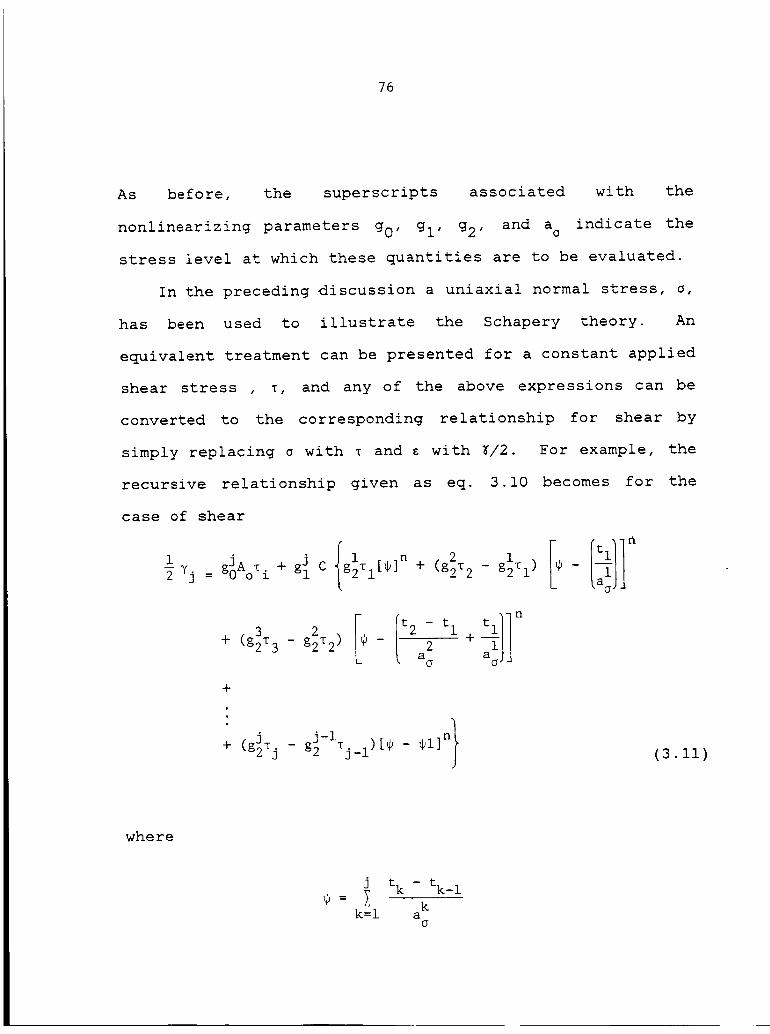
76
As before, the superscripts associated with the
nonlinearizing parameters go' gl' g2' and aa indicate the
stress level at which these quantities are to be evaluated.
In the preceding discussion a uniaxial normal stress, c,
has been used to illustrate the Schapery theory. An
equivalent treatment can be presented for a constant applied
shear stress , _, and any of the above expressions can be
converted to the corresponding relationship for shear by
simply replacing o with _ and _ with _/2. For example, the
recursive relationship given as eq. 3.10 becomes for the
case of shear
{• " i [_]n + (g_ _ g2_l) _1 _ + gl C g2rl 2 [a_J]
Yj = ggAo i
_ It2a _ t--_]]n
3 2 - tl
+ (g2_3 - g2_2 ) - +
o aojj
+
• j-I }+ (g_Tj - g2 Tj-I)[* - _l]n (3.11)
where
J tk - tk_ I
_= _ kk=l a
O
77
_i =j-I tk - tk_ I
kk--i a
Experimental Measurement of the Schapery Parameters
The above presentation has indicated that to
characterize the behaviour of a viscoelastic material using
the Schaoerv theory, s_v_ m_t_i_] m_=m=9_ :_: _:_4_:_
TL_: _: Lh= :i::Li_ _umpiiance nerm ao, _ne power law
parameter C, the power law exponent n, and the four
nonlinearizing functions of stress, go(O), gl(o), g2(o), and
ao(o). These parameters are customarily determined through
a series of creep/creep recovery tests at sequentially
higher creep stress levels. At relatively low stress
levels, linear viscoelastic behaviour is usually observed,
= 1 Therefore at low stressand hence go = gl = g2 = ao "
levels the Schapery single-integral (eq. 3.1) reduces to the
Boltzman Superposition Principle (eq. 2.2), and the Schapery
equation for creep (eq. 3.4) is equivalent to the Findley
power law equation (eq. 2.7). The results of the low stress
level creep tests can therefore be used to determine Ao, C,
and n.
Nonlinear viscoelastic behaviour is often initiated at
relatively high stress levels, and in general go # gl _ g2 _
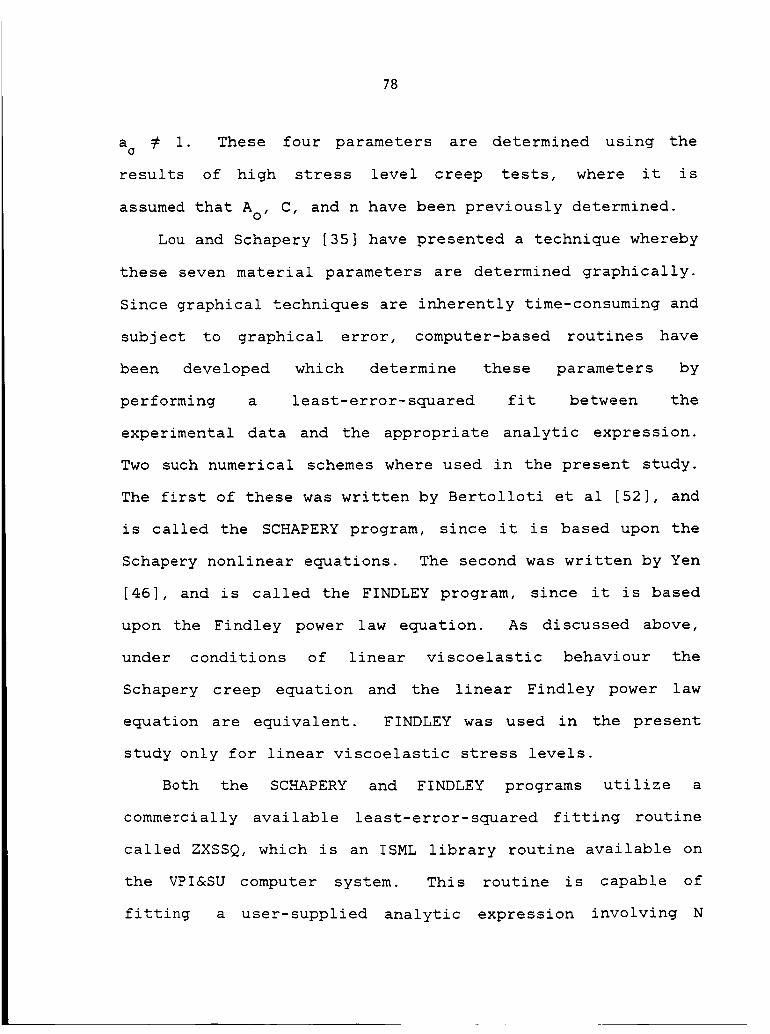
78
a _ I. These four parameters are determined using thea
results of high stress level creep tests, where it is
assumed that A o, C, and n have been previously determined.
Lou and Schapery [35] have presented a technique whereby
these seven material parameters are determined graphically.
Since graphical techniques are inherently time-consuming and
subject to graphical error, computer-based routines have
been developed which determine these parameters by
performing a least-error-squared fit between the
experimental data and the appropriate analytic expression.
Two such numerical schemes where used in the present study.
The first of these was written by Bertolloti et al [52], and
is called the SCHAPERY program, since it is based upon the
Schapery nonlinear equations. The second was written by Yen
[46], and is called the FINDLEY program, since it is based
upon the Findley power law equation. As discussed above,
under conditions of linear viscoelastic behaviour the
Schapery creep equation and the linear Findley power law
equation are equivalent. FINDLEY was used in the present
study only for linear viscoelastic stress levels.
Both the SCHAPERY and FINDLEY programs utilize a
commercially available least-error-squared fitting routine
called ZXSSQ, which is an ISML library routine available on
the VPI&SU computer system. This routine is capable of
fitting a user-supplied analytic expression involving N

79
unknowns to a set of M experimental measurements. The
details of the ZXSSQ routine are proprietary to ISML, and in
any case are irrelevent to the present discussion since
routines which can provide the same function are available
on most computer systems.
Some details regarding the SCHAPERYand FINDLEY programs
are described below.
Program SCHAPERY
The computer program SCHAPERY is used to perform two
distinct analyses, the linear viscoelastic analysis and the
nonlinear viscoelastic analysis. For the linear case three
unknowns are required; namely Ao, C, and n. For the
nonlinear case it is assumed that Ao, C, and n are known,
and the four remaining unknowns go' gl" g2' and a are
required. It is easiest to discuss the program by first
considering a linear analysis and then considering a
nonlinear analysis.
Linear Analysis. For the linear case the Schapery equations
for creep and recovery are reduced to:
_c (t) = Ao_ + Cot n (3.12)
and
_r(t ) = AEI[(I + x)n _ _n] (3.13)

80
where
&Zl = C°tl
t - t1-
t
The three unknowns in these equations are the instantaneous
compliance A o, and the power law parameters C and n.
The SCHAPERY program uses linear creep and recovery data
to determine these parameters as shown in the flow chart
given in Figure 3.3. First information defining the data
set is input. This includes the number of recovery points,
NREC, the number of creep points, NCR, the creep unloading
time, t I, the creep stress level, o, and initial estimates
for the transient creep strain, A_ I, and power law parameter
n. Note that in the linear case the transient creep strain
is directly proportional to the power law parameter C
As 1C = --
n
°0 tI
(3.1_)
Therefore, the initial estimate for Ag I is an initial
estimate for C as well.
Next the recovery data pairs are input, consisting of the
recovery time, TREC(M), and the measured recovery strain,
REC(M). The linear recovery curve, eq. 3.13, is then fit to
the data using ZXSSQ, and estimates for the two unknowns Ag I
81
InputNo. Recovery Data Pts., NREC
No. Creep Data Pts., NCR
Unloading Time, TCRIT = tlCreep Stress, SIGMA
Initial Estimates for
_I , n
IInput Recovery Data Pairs
Call Subroutine 7x_Kn
........ Eq
er(t ) : _l[(l + X) n _ Xn]
Return:
AmI : Cat_ , n
I Input Creep Data Pairs
Call Subroutine ZXSSq
Fit Linear Creep Equation:
_c(t) = _o + Cqtn
Return:
¢0 = Aoa
Figure 3.3: Flow Chart for Program SCHAPERY - Linear Analysis
82
and n are obtained. C is then calculated using eq. 3.14.
The creep data pairs are then input, TCR(M) and CR(M).
Since C and n have been determined using the recovery data,
the only unknown which remains is the instantaneous
compliance A o. The value of A ° is calculated by fitting the
creep data to the linear equation for creep, eq. 3.12, again
using the library routine ZXSSQ.
Nonlinear Analysis. In the nonlinear case, the Schapery
equations for creep and recovery are
glg2(t) = +- C tna
c g0Ao°0 n oaa
(3.15)
and
[(i + aol) n - (a k) n] (3.16)
where, for the nonlinear case,
glg2 n
Ae I = -- C an tlaa
Since it is assumed that a linear analysis has been
performed to determine Ao, C, and n, there are only four
unknowns remaining in eqs. 3.15 and 3.16. These are go' gl'
g2' and aa. Program SCHAPERY uses nonlinear creep and creep
recovery data to determine these parameters as shown in the
flow chart given in Figure 3.4. First, information defining
the data set is input, which includes the number of recovery
83
No. Recovery Data Pts., NRECNo. Creep Data Pts., NCR
Unloading Time, TCRIT = t 1Creep Stress, SIGMAInitial Estimates for
(A_i/g I ) a' 0
I
Input Recovery Data Pairs
I
Call Subroutine ZXSSQ
Fit Nonlinear Recovery Equation:
_r(t) - AcI [(I + a X) n - (aaX) n]gl a
Return:
(A_i/g I ) , aa
IInput Creep Data Pairs
I
Call Subroutine ZXSSQ
Fit Nonlinear Creep Equation:
glg2c(t) : goAoao + _ ctnao_ n
aci
Return:
(goAoao) , (glg2Cao)/(a n)
Figure 3.4: Flow Chart for Program SCHAPERY - Nonlinear Analysis
84
points, NREC, the number of creep points, NCR, the creep
stress unloading time, t I, and initial estimates for the
transient recovery strain, (AEI/gl), and the parameter a •
The recovery data pairs are then input, which consists of
the recovery time, TREC(M), and the measured recovery strain
at that time, REC(M). The nonlinear recovery curve, eq.
3.16, is then fit to the data using ZXSSQ and estimates for
the two curve-fitting parameters, (AZl/g I) and a , are
obtained.
Next, the creep data pairs are input, TCR(M) and CR(M).
The nonlinear creep curve, eq. 3.15, is then fit to the
creep data using ZXSSQ. Estimates for the quantities
n
(g0Ao_) and (glg2C_/a_) are obtained. This completes the
analysis, since all of the Schapery parameters may now be
calculated as follows:
AE1
gl = _(Ael/gl)
g2 = gl C a
85
Program FINDLEY
Since the program FINDLEY is used only for the case of
linear viscoelastic behaviour, there are only three
unknowns, Ao, C, and n. These parameters are determined
using creep data only. The creep data is fit to the Findley
power law equation
where
0+ mt n
c = A cO O
(3.17)
m = Cc
A flow chart for the FINDLEY program is given in Figure 3.5.
Information defining the data set is input first, including
the number of creep data points, initial estimates for ¢O'
m, and n, and the time and creep data sets. The Findley
power law is then fit to the data, and best-fit estimates
for ¢o' m, and n are returned. A ° and C are then calculated
using eqs. 3.17.
Average Matrix Octahedral Shear Stress
A final consideration is the effect of stress
86
No. Creep Data Pts., NCRInitial Estimates for
_o ' m , and n
Input Creep Data Pairs
iCall Subroutine ZXSSQ
Fit Linear Creep Equation:
_c (t) : _o + mtn
Return:
_o , m , and n
Figure 3.5: Flow Chart for Program FINDLEY

87
interaction in the case of multiaxial stress states. During
experimental characterization of a viscoelastic material the
various parameters are often determined under conditions of
a uniaxial normal stress. In the present case the S22(t,c )
compliance term was determined based on a uniaxial stress
_2' for example. However, an individual ply within a
composite laminate is in general subjected to a plane-stress
state consisting of the three stress components 01 , c2, and
_12" The effects of stresses °! and _!2 on viscoelastic
..... _= u,_ _ _ _t_mi_ed under uniaxial stress
a2 only must therefore be considered. Lou and Schapery [35]
and Dillard, Morris, and Brinson [21] have accounted for
such interaction through the use of the "average matrix
octahedral shear stress", _oct" This approach uses a simple
rule of mixtures approximation to calculate _oct" The
resulting expression for _oct is [21]
1
l m2 m 22Toc t : -_ [(o I - o 2) + + + 6(T12) ] (3.17)
mwhere the matrix stresses o_, 02' and _12 are given in
terms of the applied ply stresses 01 , 02, and r12 by
Imlnlo 2 =
mr12
Um- E-_I _J12
0 1
0 0
0
1
o2
r12
(3.18)

88
and
Ell = Efvf + Em(l - vf)
v12 = vfvf + _m(l - vf)
v = matrix Poisson's ratiom
Ef = fiber modulus
E = matrix modulusm
vf = fiber volume fraction
Note that it is assumed that both the ply normal stresses
perpendicular to the fibers and the ply shear stresses are
msupported entirely by the matrix, i.e., c_ = c 2 and _12
= _12"
Some of the above properties were not available for the
graphite-epoxy used in this study, as the manufacturer had
only supplied the volume fraction. The properties required
were obtained by measuring Eli, E22, and _12' and assumimg a
value form
With the additional rule of mixtures relation
E22 =
Ef Em
(i - vf) Ef + vf Em
it was possible to calculate an appropriate value for each
of the required material properties. The values obtained
and used in the analysis were
89
Eli = 132.2 GPa (19.16 X 10⁶ psi)
v12 = 0. 273
v = 0.35m
Ef = 201.3 GPa (29.2 X 10⁶ psi)
E m = 3.42 GPa (0.497 X 10⁶ psi)
vf = 0.65
The ply strain-stress relationships as used in the
I _i(t) }e2(t) =
L YI2 (t)
Sll S12 0
S12 S22(t,Toc t) 0
0 0 S66(t,TOC t
Ol(t)
O2(t)
) LZl2 (t)
(3.19)
Lamination Program VISLAP
The computer program VISLAP provides long-term
predictions of both the creep compliance and the creep
rupture times of composite laminates of symmetric layup.
This program was modified during the present study by
inserting the Schapery viscoelastic model into the program
as described above. The program will be briefly described
90
in this paragraph. The reader is referred to Reference 21
if additional details regarding program structure are
desired.
The analysis performed by VISLAP is based upon classical
lamination theory, either the Findley MSP or the Schapery
viscoelastic model, and the Tsai-Hill failure criterion
[24]. The Tsai-Hill failure criterion is normally applied
to elastic materials, but has been modified for use with
viscoelastic materials during previous research efforts
[21]. A linear cumulative damage law is used to account for
time-varying ply stresses.
A flow diagram of VISLAP is given in Figure 3.6. The
program proceeds as follows: The laminate layup and initial
lamina properties are input, (A). The current elastic
laminate strain is determined using CLT, (B) through (G).
The total laminate strain is then calculated as the sum of
the current elastic laminate strain plus the current
equivalent laminate creep strain, (H). The individual ply
stresses are next calculated, based upon the total laminate
strain minus the individual ply creep strain, (I). If the
ply stresses have changed significantly since the previous
time step, a nonlinear iteration procedure cycles through
steps (B) through (I) to assure that the ply stresses have
converged to the actual current stress state, (J). This
stress state is then stored in a stress history array and
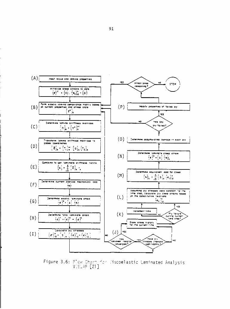
91
(A)
(B)
[(c),
I
(D)
(E)
(F)
(G)
i(H) I
1
(I) i
lnOIlt IOyUl _II1_ I|flllnl II, IOIPTIII
I lfll?llllZI ¢TI19 Ill'GinS ?0 ZlITO
[ {,}: . {°}. r,_,,,,_'"{o}
j _'lll'lII IIIili'1(: Iomlnl ¢111_|111n¢1 m¢llrll OtllllO=I,ITTIIfl& _ml_ll_lll| OI_CI SYrllUL Slqf41
I [,'3,i
_IIIIITIIlIIItl IOllllqll ifl_TIIIIl| PTI4TTICII
IT
TcQnstQfm :Qmlll_ 2tT+PI'IIII l?lOlr1¢ll TQ !
+IOOlll 2.00fO| hOtll I
i+j, ,+-:-++ ' F-"•;',J.LQJ."zJ.
_._mOlnll tO QII& h_lmlflQtl Stlf_Pll1111 _¢It,_l 1
_iII
_IIflITTTIII'III _frlll_ _& 3001110 _l_l¢,'IOTlle'=l IOQ_
_41fllr_ln4l ltO|l'l¢ lOTfllqlOfll StT'_ll_l
_lltllrmll_l TOtal lQmlnOTll strgln !
{,}"{+}'-{,i" Ir
':..IlCu*OTII _17 srreClel i
( _" " . . .• + =' +(_' - " , + ,
p---
fiI
(p) _o:,,, o,:o..,.. °,,.,,.. :.,
--..<,: ,o..o._"T
(o/I-+-. =°+°°.,,.oo o.,t
_lltllfl_lll_ _l_llrlOtll ¢TllllO StTI_ITI
(N) +,,'" .+_'_ , ,
IJ _4&ITml_lll 41QU_VCIIeTI& iO_CI #_r _ llllO
i ,( ° ,(M) , {_},".-'. :i,' :.:/,,"
t•_SSUIS_lflq _ly sTr_ISS41S _llfll =::nS't_l_f +::M" _+'ll
?lffll $_+llr_, _I¢I.lt_[TI _ly =.+_O0 StTCIInS "_QIIM'CI
(L) +" '"" _°"'"'""'" _'"°"°"',,+ .t2
(K)
_t¢ll'll $tTIIIII _vStOry :
! .... :
__o.+(d)"' _ I
Figure 3.6- F_c;.; Sh:-:-- _c, 'iscoelastic Laminated AnalysisVZ_' '_ [21]

92
time is incremented, (K). The current ply creep strains
which would be produced by the stresses stored in the stress
history array are then calculated, (L). The modified
version of VISLAP allows the user to select either the
Findley MSP viscoelastic model or the Schapery viscoelastic
model to calculate these ply creep strains. An "equivalent
mechanical load" which equals the summation of the loads
required to produce ply elastic strains of the same
magnitude as the current ply creep strains is next
calculated (M). This equivalent load is then used to
calculate the equivalent laminate creep strain (N). The
modified Tsai-Hill failure criterion is used to predict any
lamina failures, together with the cumulative damage law and
the stress history array. Should a ply fail, the ply
properties are modified to account for the type of ply
failure (i.e., either a fiber or a matrix failure), (O) and
(P). The entire procedure is repeated until either all
plies have failed or the user-specified maximum time is
reached.
A subtle point in the analysis which should be noted is
that the equivalent laminate creep strains calculated in
step (N) do not in general equal the individual ply creep
strains calculated in step (L). The differences between the
equivalent laminate creep strains and the individual ply
creep strains are added to the original elastic ply strains,

93
resulting in ply stresses which vary with time. As
viscoelastic deformations occur, a greater percentage of the
externally applied loading is supported by the fibers,
whereas the matrix load is decreased. Thus, the ply
stresses change with time even though the externally applied
creep load is constant.
IV. SENSITIVITY ANALYSIS
Early in the experimental portion of this study, it
became apparent that the linear viscoelastic parameters A o,
C and n were very sensitive to small errors in measured
strain data. High sensitivity to measurement errors have
also been reported by Dillard [21], Hiel [22], Rochefort
[37], and Yen [46]. Both Dillard and Yen concluded that a
stable value for the power law exponent n could not be
obtained through short-term creep tests; long-term tests of
a duration of 104 minutes (6.9 days) or greater were
required. The major difficulty encountered by Hiel during
his application of the Schapery theory was that "damage"
accumulated within the test specimen during the creep
portion of the creep/creep recovery testing cycle. This
resulted in a permanent strain reading after the recovery
period, i.e., the recovery strains did not return to zero
but rather approached some permanent strain level in an
asymptotic manner. Similar difficulties have been discussed
by others, including Lou and Schapery [35], Caplan and
Brinson [36], and Peretz and Weitzman [50]. From these
efforts, it appears that damage accumulated during the creep
portion of the testing cycle is the major potential source
of error in application of the Schapery theory. Hiel used
his recovery data to calculate various viscoelastic
94
95
parameters, but could obtain stable values only by first
subtracting the permanent strain from the recovery data
recorded at each point in time. This procedure effectively
translates the entire recovery curve down towards zero
strain.
It should be noted that many researchers subject
viscoelastic specimens to a "mechanical conditioning cycle"
prior to the creep/creep recovery test [35,37,46]. The
assumption is that such a conditioning cycle produces a
stable damage state within the specimen, and no further
damage is accumulated during the creep/creep recovery test.
Apparently this approach avoids the difficulties associated
with permanent recovery strains encountered by Hiel.
However, Hiel argues [22] that mechanical conditioning
results in a fundamental change in the material being
investigated, and therefore results obtained from
mechanically conditioned specimens do not reflect the
behaviour of the material which would occur in a practical
situation. Specifically, it was felt that mechanical
conditioning results in plastic deformation of the matrix
material which alters the initial stress-strain constitutive
relationship of the virgin matrix material. A further
complication arises in the present case, since results
obtained using unidirectional specimens were to be used to
predict the response of laminates with arbitrary layup.
96
Since ply stress states vary with layup, the appropriate
mechanical conditioning cycle would depend upon the specific
laminate being studied. Due to the above considerations, no
mechanical conditioning was performed in the present study.
Two areas of concern arose during the present efforts
due to the above observations. First, the level of accuracy
required when determining the values of the seven Schapery
viscoelastic parameters was not clear. Since these
parameters were to be used to predict long-term viscoelastic
behaviour, such errors could obviously impact the predicted
response. Therefore, until the impact of these errors on
predicted response was evaluated, the severity of such
errors could not be properly appreciated. Secondly, it
appeared that some viscoelastic parameters were more
sensitive to experimental error than others. For example,
the values obtained for the power law exponent n by Dillard
[21] at various stress levels exhibited a significant
scatter, whereas the values for the power law parameter m
(where in the linear case m = Ca) were relatively smooth and
uniform with stress (see Figure 1.3). An attempt was made
to determine the origin of this sensitivity. It was felt
that such information would indicate the level of stability
which could be expected for each parameter during reduction
of actual experimental data, and might also be useful in
selecting appropriate testing cycles and data reduction
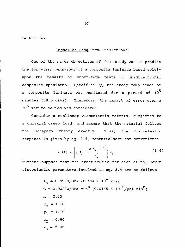
97
techniques.
Impact on Lonq-Term Predictions
One of the major objectives of this study was to predict
the long-term behaviour of a composite laminate based solely
upon the results of short-term tests of unidirectional
composite specimens. Specifically, the creep compliance of
a composite laminate was monitored for a period of 105
minutes (69.6 days). Therefore, the impact of error over a
105 minute period was considered.
Consider a nonlinear viscoelastic material subjected to
a uniaxial creep load, and assume that the material follows
the Schapery theory exactly. Thus, the viscoelastic
response is given by eq. 3.4, restated here for convenience
lg glg 2 C tec(t ) = 0A ° + _ o0 (3.4)
a n
Further suppose that the exact values for each of the seven
viscoelastic parameters involved in eq. 3.4 are as follows
A ° = O.0978/GPa (0.674 X lO-6/psi)
C = O.O0210/GPa-min n (0.0145 X lO-6/psi-min n)
n = 0.33
go = I.i0
gl = I. I0
g2 = 0.90
a = 0.90O
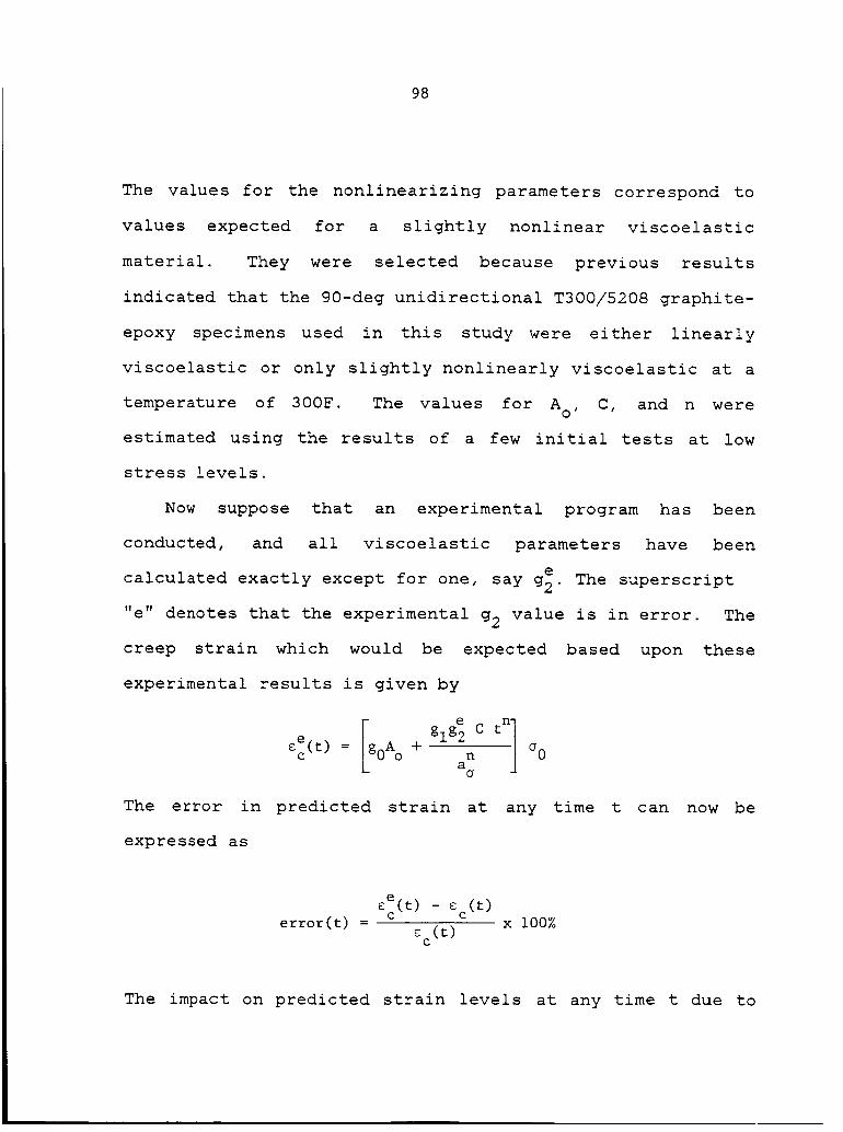
98
The values for the nonlinearizing parameters correspond to
values expected for a slightly nonlinear viscoelastic
material. They were selected because previous results
indicated that the 90-deg unidirectional T300/5208 graphite-
epoxy specimens used in this study were either linearly
viscoelastic or only slightly nonlinearly viscoelastic at a
temperature of 300F. The values for Ao, C, and n were
estimated using the results of a few initial tests at low
stress levels.
Now suppose that an experimental program has been
conducted, and all viscoelastic parameters have been
calculated exactly except for one, say g_. The superscript
"e" denotes that the experimental g2 value is in error. The
creep strain which would be expected based upon these
experimental results is given by
eglg 2 C t_-(t) = +
O 0c- - n
a o
The error in predicted strain at any time t can now be
expressed as
ee(t) - e (t)
error(t) c c= x 100%(t)
C
The impact on predicted strain levels at any time t due to
99
an error in one of the viscoelastic parameters can be
isolated using this approach. Based upon previous results,
a deviation of _I0_ from the average measured value of the
linear viscoelastic parameters is not uncommon, so this
level of error was used in the analysis. A creep stress
level of 13.8 MPA (2000 psi) was assumed.
Note from eq. 3.4 that go and A° are both linearly
related to the creep strain _c(t), and therefore a !I0_
error in either go or A ° has the same affect on _c(t).
Similarly, _I0_ errors in g1' g_' or C affect the predicted
creep strains in identical fashion. Therefore, only four
analyses were required: the first to account for errors in
go or A o, the second to account for errors in gl" g2' or C,
the third to account for errors in n, and the fourth to
account for errors in a
Results are summarized in Figures 4.1-4.4. Figure 4.1
illustrates the error in predicted creep strains due to a
_i0_ error in either go or A o. An error of this type is
confined entirely to the instantaneous creep strain, i.e.,
the transient creep strains are not affected by an error in
either go or A o. Therefore, the percentage error is equal
to !10% at time t = O, and slowly decreases with time as
transient strains develop. After 105 minutes, the error has
been reduced to about _7_.
The effects of a _I0_ error in gl' g2' or C are
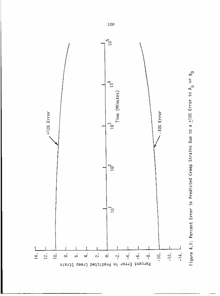
i00
I I
c_
0
-- 0
0_-- 0
-- 0
0
LLJ
0
p....I
I
_" 'T
0
t_0
0
.r,-
0
_,_
0
+1
0
"_,
.r-"
e_
-r--
0
.°

i01
i,i
+
uL_a_S da_a_ pa_paad uL a0aa3 _u_a_d
¢xa
S-0
G
,p-
L0
0
"7",,
0
%
m
0j
u.p-
.r'-
0
E
U
g
.r,-
I.u.
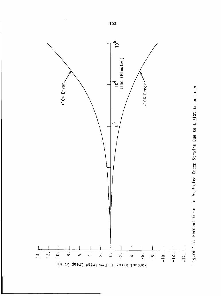
102
I I
oJ
I [ I I I I I I
I I I
u_ea%S da_a3 Pa_Lpaad uL aoaaH _u_Da_ d
I
o_I
I I
C"
.t-
OS..S-L_
0
e--+1
0
E
U.r--
E.i--
0
LIJ
4-_
r_
°.
| ._-.kL

103
u_eJ_S deaa3 pe%9_paad uL _o_J3 _uag_ad
_b
e,-°_
K-0i.K-
0p-.
+1
0
c'-
"V_
_')
t_U
_J-IJ
,p-
c'-
._I
0¢,._
t_
J
L
°r I
104
illustrated in Figure 4.2. Since an error of this type
impacts only the transient component of the total creep
response, the percentage error is very low at short times,
and in fact is zero at time t = 0. As indicated, the
percentage error reaches !3% after 10 5 minutes.
Figure 4.3 illustrates percentage error due to a _I0_
error in n. This error again impacts only the transient
strain response, and hence the error is very low at short
times. At long times however, the error becomes appreciable
and obviously increases dramatically for times greater than
10 5 minutes. A I0% error in n results in a 12% error in
(t) after 10 5 minutes, while a -I0% error in n results inc
a -9% error in _ (t) after 10 5 minutes.c
A _I0% error in a ° is illustrated in Figure 4.4. The
error curve for a is very similar to that for error in n,o
but as indicated the predicted values for _c(t) are much
less sensitive to error in a than to error in n. The erroro
in Ec(t ) due to a +10% error in a° is less than $1% after
10 5 minutes.
It should be noted that Figures 4.1-4.4 are based upon
the specific values selected for A o, C, n, go' gl" g2' and
ao. Different results would obviously be obtained if the
material properties were different, and the results reported
here should not be considered to be representative of the
response of all viscoelastic materials. It is considered

105
that the results presented are reasonably accurate for a
90-deg unidirectional specimen of T300/5208 graphite-epoxy,
however.
Sensitivity to Experimental Error
In this paragraph, efforts to determine which of the
viscoelastic parameters are most sensitive to experimental
error will be described. As presented in Chapter III, these
seven parameters are determined using a two-step process.
First Ao, C, and n are calculated using creep and recovery
data obtained at relatively low stress levels such that
linear viscoelastic behaviour is observed. Once estimates
for Ao, C, and n are obtained the remaining four parameters
go' gl' g2' and a ° are determined using nonlinear data
recorded at higher stress levels. The sensitivity analysis
followed this same format. An analysis was first performed
which considered the sensitivity of Ao, C, and n to errors
in linear viscoelastic data. A second analysis then
considered the sensitivity of gO' gl' g2' and a° to errors
in nonlinear viscoelastic data.
The first step in both analyses was to generate an
"exact" creep and creep recovery data set. This data set
was generated analytically using the Schapery equations.
That is, strain data were calculated at specified times
using eqs. 3.4 and 3.8 and subsequently used as the exact

106
data Set. Values assumed for the various viscoelastic
parameters were the same as those listed in the preceding
paragraph, and as noted are appropriate for a slightly
nonlinear viscoelastic material. A 30 minute/60 minute
creep/creep recovery testing cycle was assumed. A testing
cycle of this duration is typical of those used in previous
studies [18-22,35-37,46,50,51]. During the present study, a
480 minute/120 minute creep/creep recovery test cycle was
used, partially due to the results of the present
sensitivity analysis. Selection of the testing cycle
employed in this study will be further discussed in Chapter
V.
Once the exact data was obtained as described above, it
was neccessary to define the errors within the data set.
Two types of error were considered, a "percentage error" and
an "offset error". For the percentage error case, the
strain data used in the analysis was in error by some
constant percentage of the exact strain value at each point
in time. The +I0% error case for creep recovery is shown in
Figure 4.5. Note that a percentage error causes a change in
shape of the strain history curve, since the numerical value
of the error changes as the value of the exact strain data
changes.
For the case of an offset error, the strain data used in
the analysis was in error by some constant amount at any

107
0 0
. t__ I
(UL/U_n) u_J_S _J_AO_a_
I
//i
/
00 ,---_o +l
c"
_ °r'-
E m•r.,- *
,_ q.I E
-- >°p-
c'-.T,-
m
m
0
m°r,.--'r-
E
-g
O 0
¢.y._
d-;g
*r.--LL
108
time. That is, some constant strain value was added to or
subtracted from the exact data set at all times. The +5
_in/in offset error case is shown for creep recovery in
Figure 4.6. An offset error does not change the shape of
the strain history curve, but rather rigidly translates the
entire curve up or down the vertical axis. Note that Hiel
[22] reduced his recovery data as if an offset error had
occurred. That is, the permanent strain reading recorded
after recovery was subtracted from the recovery strain data
at each point in time, translating the entire curve down the
strain axis.
Both the percentage and offset error types have been
defined as an artificially smooth deviation from exact
behaviour. Simple random error probably occurs most
frequently in practice, where "random error" refers to small
errors in strain measurement which occur in no discernible
pattern and at intermittent times throughout the test
period. Due to their very nature, random errors are
difficult to model. The effects of random error are most
often accounted for through the use of some least-error-
squared smoothing technique. Such techniques were used
during the present study as described in Chapter III, to
minimize the effects of any random experimental error.
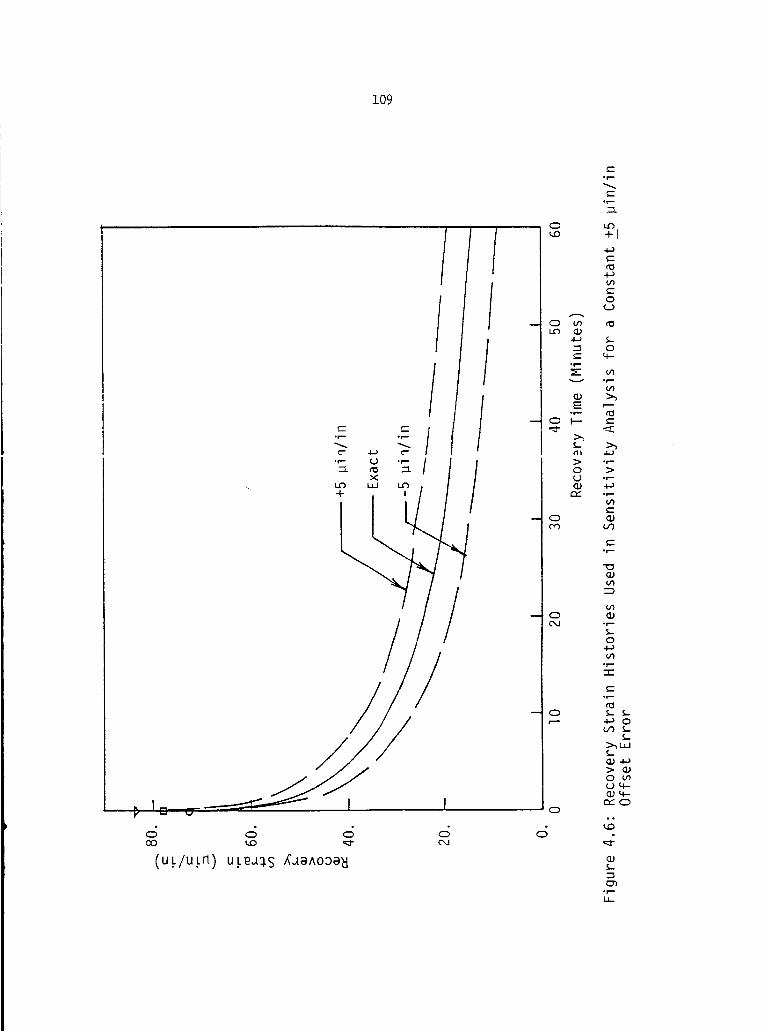
109
//
0
-- 0 ¢n
e-.r-
t-,r--
U_
+I
c-
o0c-O0
i-
0
/
!
c" q--°_
E
-- 0 t--" E
_ .r--0 _¢,J .r-
C--°r"
VI
,p
04--}C_
.r--"r"
o-
r'- 4_ 0
L(l.J -_
c; d:;g
.p

ii0
Linear Viscoelastic Analysis
As discussed in Chapter III, two computer-based fitting
routines were available to obtain the linear viscoelastic
parameters Ao, C, and n. The SCHAPERY program utilizes
linear creep recovery data to calculate C and n, and linear
creep data to calculate A o. The FINDLEY program uses only
linear creep data to calculate A o, C and n. These programs
were used to generate the results presented below.
Calculations Using Creep Data. A o, C, and n were calculated
using creep data which contained percentage errors ranging
from -I0_ to +I0_. The results of these calculations are
summarized in Figure 4.7. It was found that n is completely
independent of percentage errors, as n was calculated
correctly as 0.33 in all cases. A 0 and C were influenced
dramatically by percentage errors, however. Furthermore, it
was found that a percentage error in strain data causes the
same percentage error in A and C. For example, a +i0_o
error in strain measurement causes the same +I0_ error in
both A and C.o
A o, C, and n were next calculated using creep data which
contained offset errors ranging from -I00 _in/in to +I00
_in/in. These results are summarized in Figure 4.8. It was
found that both C and n are independent of offset errors in
creep data, and all error is confined to the estimate for
A o. This is as would be expected, since as previously noted
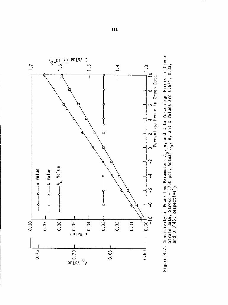
iii
0
III I I I
0
0anL_A V
_0
I
I
0
Q;Q_
c_
rDr--_ or'-,.
_D_
¢.- U "_0 _,--
0_.._
_ "T"I
U
.%_ e'_
l:_.. 0
¢_ .r-
_ mU
4-_ cn
o_
,-- _-
.°r_

112
hO_0
0
'=T
CD
n3 >> >
0¢- __) <
(__OL x)0
r--"
I
P_
I I I
an L_A 2),__
c
0",:::t-
r---
I
[
, I
I
cO0 CO '._o") 0.1 O.J
an L_A u
I I
0an L_A V
L_
O_
0
0CO
°w--
c-.r-
v
e-l 0 ";--
tO
oO
CO
-- 0 c-
O
1,1
-- 04--
' 0
-- 0
I
-- 0
I
-- 0
O0I
00
C,l
C__ r--_0_D
"0c" _"
°r- _
_g
4-_ _
C"
C" C"
¢._
E
r0_J
o
4-o
°_.-
°r-
La_
<
4-_
<
0
II
_') r"-
_- >
_D
113
an offset error does not change the shape of the creep curve
but merely shifts the entire curve up or down the vertical
axis. Hence, only the estimate for the initial compliance
A is affected. These results imply that even in the caseo
of very high offset error accurate measurement of C and n is
possible using creep data.
Calculations Using Recovery Data. The parameters C and n
were calculated using recovery data which contained
percentage errors ranging from -I0_ to +I0_. The results
are summarized in Figure 4.9. As before, it was found that
n is completely independent of percentage errors, while C is
linearly dependent on percentage errors; a +I0_ error in
strain measurement causes a +I0_ error in the calculated
value for C.
In Figure 4.10 the estimates for C and n calculated using
recovery data which contained offset errors ranging from -5
kin/in to +5 _in/in are shown. It is seen that both C and n
are highly sensitive to offset errors in recovery strain
data. This is in direct contrast with the results presented
in Figure 4.8, where it was shown that offset errors
imbedded within linear creep strain data had no effect on
the estimates for C and n, but only on the estimate for A o"
These results indicate that estimates for C and n may be
more stable if obtained by using creep data rather than
recovery data, especially under conditions in which offset
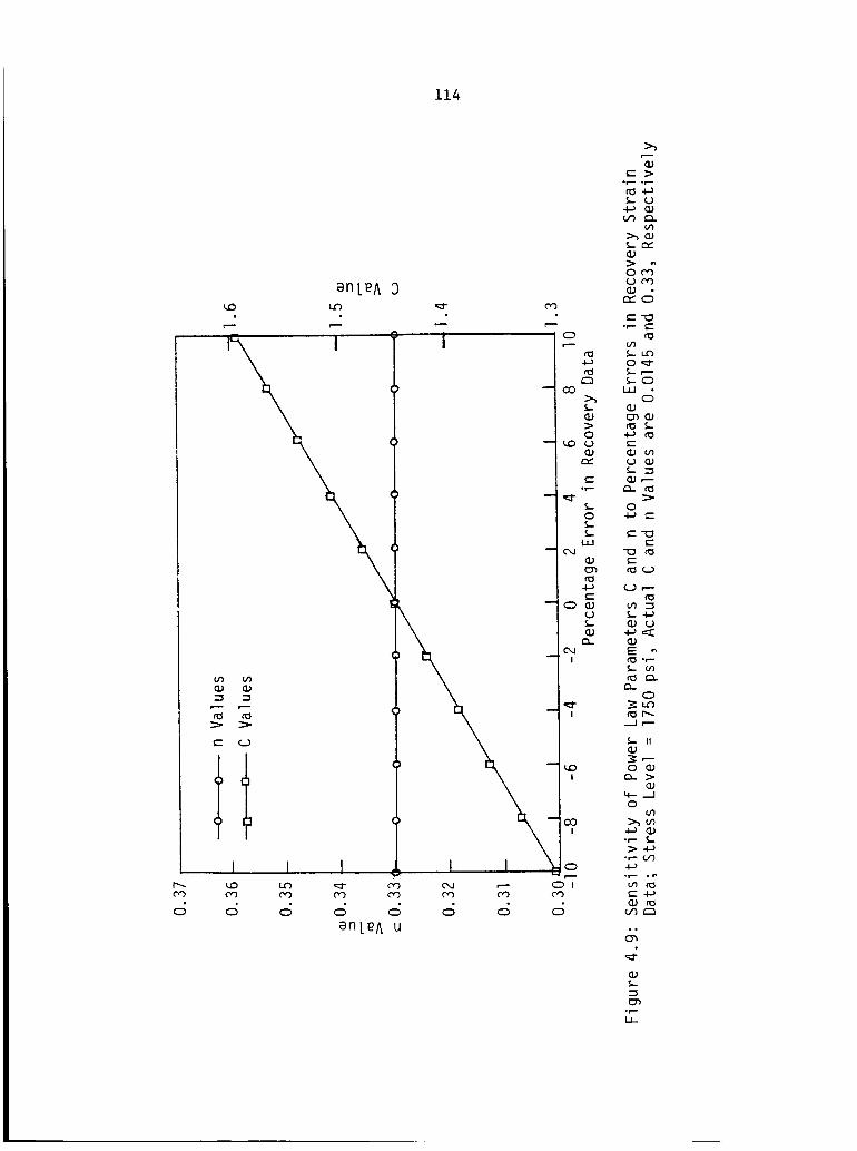
114
oO
an L_A :3
I I I
c; c;
I
I I
an L_A u
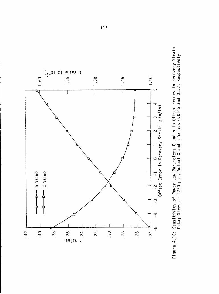
115
C_
X) anL_A O
\
O
I
lIC:0
I
an LeA u
l I
CO
!
¢-
_.l--f,-._0 U
0 Q-U u_0
t_t_
:g°r--
_sQ
__ c-
_4--. O
O m
e-_.--
to E
Em _
E _
L
3m
Qm
_m
°r-- _._-4J
•,- _,,
C¢-) r'-'_
°p-

116
errors may be prevalent.
Nonlinear Viscoelastic Analysis
During the nonlinear viscoelastic analysis, the impact
of measurement error on the four nonlinearizing parameters
go' gl' g2' and a° were investigated. It was assumed that
the exact values for A o, C, and n were known, and the
program SCHAPERY was used to calculate the effects of the
two types of error considered.
Effects of Percentage Errors. The effects of percentage
errors ranging from -I0_ to +I0% are summarized in Figures
4.11-4.14. As indicated, the parameters go and g2 are most
sensitive to percentage errors. The variance of go with
percent error was found to be linear, and is very similar to
the effects on A in the linear case (see Figure 4.7). Thiso
simply reflects that error in the initial response is
embedded entirely within the go parameter. Errors in the
transient response are divided among the gl' g2' and a °
parameters in a manner dictated by the least-squared-error
convergence criteria within the program SCHAPERY. This
accounts for the rather irregular dependence on percent
error exhibited by these three parameters.
Effects of Offset Error. Offset errors were expected to
arise mainly due to accumulated damage within the matrix
material. Such damage becomes apparent during the recovery
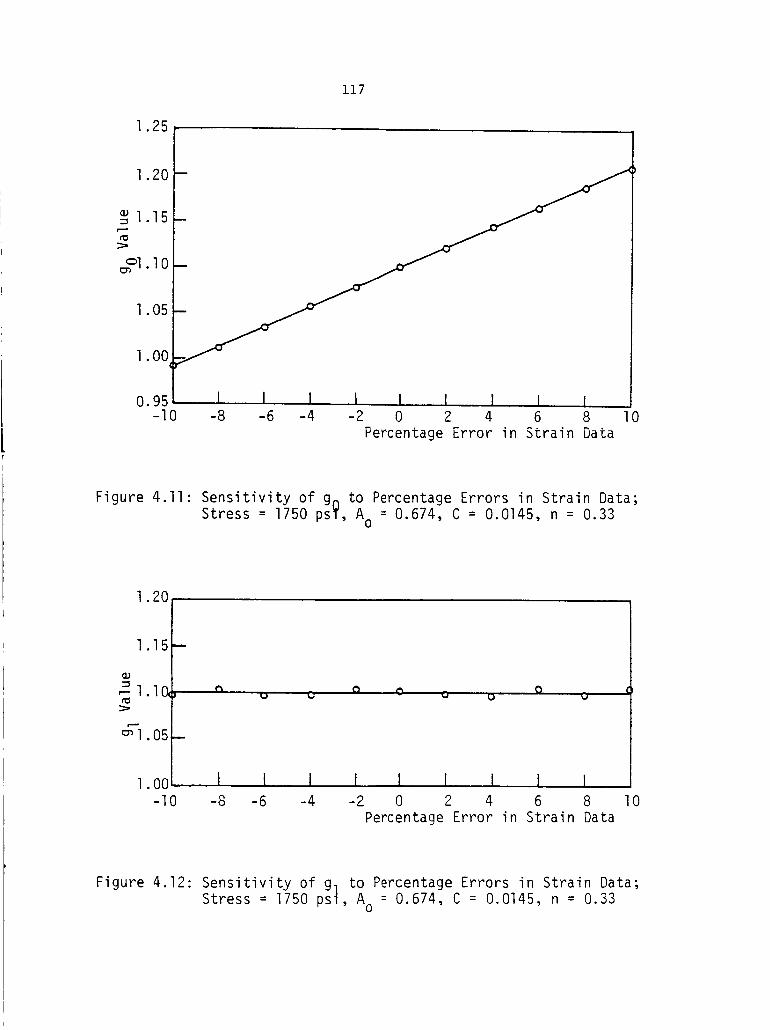
117
1.25
1.20
_1 15
_I lO
l 05
l O0
0.95-I0
; I I I I I l I I-8 -6 -4 -2 0 2 4 6 8 I0
Percentage Error in Strain Data
Figure 4.11: Sensitivity of gn to Percentage Errors in Strain Data;Stress = 1750 psT, A = 0.674, C = 0.0145, n = 0.33
o
1.20
1.15
=I I0_°
_1.05-
1. O0-10
I I I I I I-2 0 2 4 6 8
Percentage Error in Strain Data
Figure 4.12: Sensitivity of gl to Percentage Errors in Strain Data;
Stress = 1750 psi, Ao -- 0.674, C = 0.0145, n = 0.33
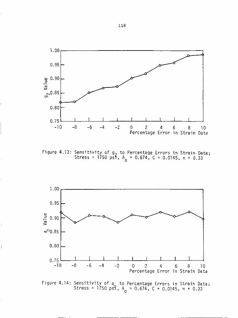
118
1.00
0.95
0.90
i_0.85
0.80
0.75 I I I I
-I0 -8 -6 -4 -2
I l I I I
0 2 4 6 8 I0Percentage Error in Strain Data
Figure 4.13: Sensitivity of g_ to Percentage Errors in Strain Data;
Stress = 1750 pst, A° = 0.674, C = 0.0145, n = 0.33
1.00
0.95
0.90
_0.85
0.80 I
0.75-I0
I i I I-8 -6 -4 -2
I I I I I
0 2 4 6 8 I0Percentage Error in Strain Data
Figure 4.14- Sensitivity of a to Percentage Errors in Strain Data;0145, nStress = 1750 psi, Ao 0.674, C = 0 = 0.33

119
portion of the creep/creep recovery testing cycle in the
form of a permanent strain reading. If this permanent
strain is subsequently removed from the recovery data, the
offset error within the recovery data is presumably
decreased to a relatively low level. However, since the
mechanism by which damage is accumulated during creep is not
apparent, no correction of the creep data has been performed
during previous efforts. The offset error within the creep
data therefore remains relatively high.
These considerations were taken into account by
specifying different levels of offset error in the creep and
creep recovery data. Offset errors ranging from -i00 _in/in
to +I00 bin/in were assumed to exist within the creep data,
while offset errors ranging from -5 _in/in to +5 _in/in were
assumed to exist within the recovery data. While specifying
offset error in this manner is admittedly arbitrary, it is
believed to reflect the qualitative nature of offset errors
which would exist in an experimentally obtained data set.
The results of this analysis are presented in Figures
4.15-4.18. The major impact of the offset errors considered
is embedded within the parameters go and a , although all
four parameters are affected to a greater extent by offset
errors than by percent errors.
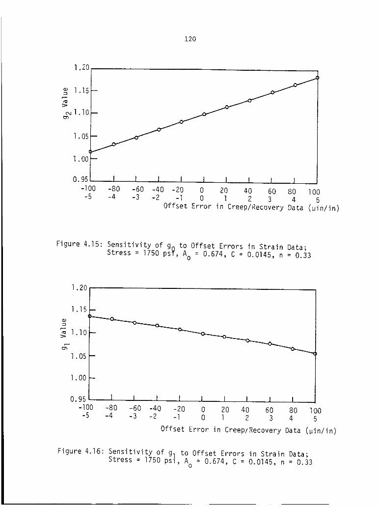
120
1.20
1.15
gl lO
1 05
i
1 O0
0.95 I-I00 -8O
-5 -4
I I I I I I I I
-60 -40 -20 0 20 40 60 80 I00-3 -2 -I 0 1 2 3 4 5
Offset Error in Creep/Recovery Data (_Jn/in)
Figure 4.15: Sensitivity of gn to Offset Errors in Strain Data;
Stress = 1750 psT, Ao = 0.674, C = 0.0145, n = 0.33
1.20
1.15
__1 10
1.05
1.00 -
0.95-I00
-5
m
I
-80-4
I I I I I I I I
-60 -40 -20 0 20 40 60 80 I00-3 -2 -I 0 1 2 3 4 5
Offset Error in Creep/Recovery Data (_in/in)
Figure 4.16" Sensitivity of gl to Offset Errors in Strain Data;Stress = 1750 psi, A = 0.674, C = 0.0145, n = 0.33
0
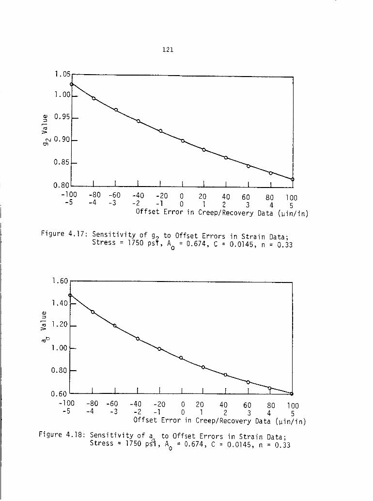
121
1.05
¢
1. O0
0.95
0.90
0.85
0.80
-I00-5
m
I _ I I J 1 l l l_
-80 -60 -40 -20 0 20 40 60 80 I00-4 -3 -2 -I 0 1 2 3 4 5
Offset Error in Creep/Recovery Data (win/in)
Figure 4.17- Sensitivity of ge to Offset Errors in Strain Data;
Stress = 1750 psi, A° = 0.674, C = 0.0145, n = 0.33
1.60
I
1.40
"_ 1.20
1. O0
0.80
0.60
-I00 -80 -60-5 -4 -3
-40 -20 0 20 40 60 80 I00-2 -I 0 1 2 3 4 5
Offset Error in Creep/Recovery Data (win/in)
Figure 4.18: Sensitivity of a to Offset Errors in Strain Data;
Stress = 1750 p_, A° = 0.674, C = 0.0145, n = 0.33
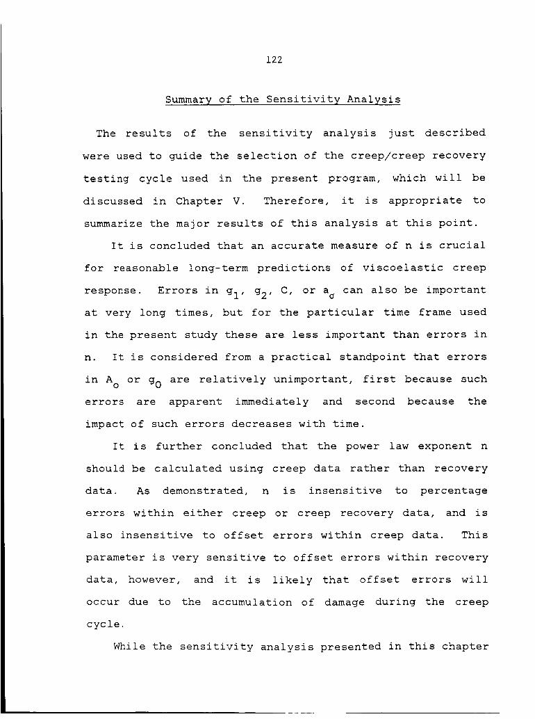
122
Summary of the Sensitivity Analysis
The results of the sensitivity analysis just described
were used to guide the selection of the creep/creep recovery
testing cycle used in the present program, which will be
discussed in Chapter V. Therefore, it is appropriate to
summarize the major results of this analysis at this point.
It is concluded that an accurate measure of n is crucial
for reasonable long-term predictions of viscoelastic creep
response. Errors in gl' g2' C, or a ° can also be important
at very long times, but for the particular time frame used
in the present study these are less important than errors in
n. It is considered from a practical standpoint that errors
in A ° or go are relatively unimportant, first because such
errors are apparent immediately and second because the
impact of such errors decreases with time.
It is further concluded that the power law exponent n
should be calculated using creep data rather than recovery
data. As demonstrated, n is insensitive to percentage
errors within either creep or creep recovery data, and is
also insensitive to offset errors within creep data. This
parameter is very sensitive to offset errors within recovery
data, however, and it is likely that offset errors will
occur due to the accumulation of damage during the creep
cycle.
While the sensitivity analysis presented in this chapter
123
is believed to represent a reasonable approach, it must be
admitted that rather arbitrary and subjective assumptions
have been made. These are necessitated for the most part by
the unknown nature of the damage mechanism believed to be
primarily responsible for experimental error. Until further
information regarding such damage is available, a more
rigorous sensitivity analysis cannot be performed.
V. SELECTION OF THE TESTING SCHEDULE
Preliminary Considerations
The
Schapery
determined
seven viscoelastic parameters involved in the
nonlinear viscoelastic theory are typically
using data obtained during a series of
creep/creep recovery tests. The testing schedule used to
determine these parameters must be selected so as to insure
that the viscoelastic response predicted at long times is
reasonably accurate. This is especially significant in
light of the analysis presented in Chapter IV, where it was
demonstrated that an error in any of the parameters
associated with the transient response (gl' g2' ao" C, or n)
is not apparent at short times but may result in gross error
at long times. This implies that prior to selection of the
creep/creep recovery testing cycle a conscious decision must
be made regarding both the desired length of prediction and
desired accuracy of prediction. A testing cycle which
results in an acceptable prediction at 10 5 minutes may not
result in an acceptable prediction at 10 6 minutes, for
example.
A review of the literature indicates that in general the
creep/creep recovery testing schedules used during previous
applications of the Schapery theory have been of relatively
124
125
short duration. For example, some reported creep/creep
recovery time schedules are 60 minutes/600 minutes [22], 60
min/120 min [35], 30 min/30 min [36], 30 min/60 min [37], 15
min/5 min [50,51], and 25 min/25 min [53]. In all studies
the viscoelastic response was compared to actual
measurements and judged to be an accurate prediction.
However, in all cases the predicted response was compared
over a time span either equal to or only slightly greater
than the original creep time. Thus, it is not clear whether
testing schedules listed are accurate enough to provide
viscoelastic predictions at much longer times, say at times
greater than 104 minutes.
Another consideration is the method of strain
measurement used. In this study (and in most previous
studies) resistance foil strain gages were used to measure
strain. In modern strain gage applications, the strain gage
system (including strain gage, amplifier, and readout
device) will commonly provide a sensitivity of 1 _in/in.
However, there are many inevitable experimental difficulties
involved, including amplifier nonlinearities, instabilities,
and noise; strain gage thermal compensation; strain gage
stability and drift; and tolerances in gage factor and
resistance. When these factors are taken into account,
measurement accuracy under the best of conditions is
126
probably no better than about _5 _in/in. This potential
level of error must also be considered during selection of
the test cycle.
The amount of viscoelastic response expected at the
temperature and stress levels of interest is also of
importance. In general, long-term predictions for highly
viscoelastic materials require a very accurate measure of
the viscoelastic parameters, whereas predictions for mildly
viscoelastic materials require less accurate measurement of
these parameters.
A final consideration is applicable for the specific
case in which the transient compliance is modeled using the
power law (as in the present study). The power law is
merely a good approximation to the actual transient
compliance function. While the power law is reasonably
accurate for many viscoelastic materials, it cannot provide
an exact match with measured results at all points in time.
Since in practice the viscoelastic response at long times is
generally of greatest interest, it is desirable to provide
the best fit between analytic and experimental results at
long times. Accuracy at long times is often accomplished at
the expense of accuracy at short times, however.
Testing Schedule Selected
The test schedule used during this study was selected

127
with several objectives in mind, in light of the above
considerations and the results presented in Chapter IV. The
schedule was keyed towards an accurate measure of the power
law exponent n. The selection process is described below.
Initial estimates for the linear viscoelastic parameters
A o, C, and n were obtained by conducting a few 30 min/60 min
creep/creep recovery tests on a 90-deg specimen of T300/5208
graphite-epoxy. The results of these tests were used in the
sensitivity study presented in Chapter IV, and the estimates
obtained are restated here for convenience
A ° = 0.0978/GPa (0.674 X 10⁻⁶/psi)
C = 0.O0210/GPa-min n (0.0145 X lO-6/psi-min n)
n = 0.33
The linear viscoelastic creep response at any time t is
given by eq. 3.4 (with go = gl = g2 = ao = I)
ec(t) = [A° + C tn] o0 (5.1)
Equation 5.1 can also be rearranged to provide an expression
for n, in terms of Ao, C, n, t, and _(t)
olln =
log t
The approximate creep strain expected at 105 minutes for
(5.2)
T300/5208 was calculated using eq. 5.1 and the initial
estimates for A o, C, and n, at a stress level 12.1MPa (1750
128
psi). The viscoelastic response was expected to be linear
at this stress level. The approximate creep strain was
calculated as
g(105) = 2313 uin/in
Next, an accuracy of !10% at 105 minutes was specified.
That is, the measured value of n was required to produce a
predicted creep response within 110% of the actual creep
strain at 105 minutes. A !10% error implies a predicted
response at 105 minutes of
g(I05)+i0% = 2544 _in/in
_(I05)_i0% = 2082 _in/in
The error bounds on n can now be calculated using eq. 5.2
n+10% = 0.346
n_10% = 0.310
Since the "exact" value of n is assumed to be 0.33, the
specified _I0_ tolerance on predicted creep strain at 105
minutes requires that the error in n range between -6.1% to
+4.8%. Therefore, the creep time used to determine n must
be long enough such that this difference in n can be
distinguished. As previously discussed, the accuracy in
strain gage measurements is perhaps +5 _in/in. It was

129
arbitrarily decided to specify a confidence level in strain
measurement of +20 _in/in for the present study. That is,
the creep time was to be long enough such that a variance of
+20 _in/in away from "exact" behaviour could be measured.
It was reasoned that this rather conservative confidence
level would help to assure an accurate measure of n. The
transient response given by each value of n has been plotted
in Figure 5.1. As indicated a variance of !20 _in/in away
from the response for n = 0.33 occurs at about 480 minutes.
The duration of the creep test chosen for this study was
therefore 480 minutes.
Once the length of the creep test was selected it was
possible to specify a reasonable recovery period. The
predicted recovery curves following 480 minutes of creep at
12 1 MPa are o_ .... in Figure 5 2 Since _..... w....... e material has
been assumed to be linearly viscoelastic, the variance from
the n = 0.33 curve is initially +20 _in/in. After 120
minutes this variance has been reduced to about +13 _in/in.
This was judged to be a reasonable recovery time, and so
recovery strains were monitored for 120 minutes.
In summary, the creep/creep recovery testing cycle used
in this study was keyed towards accurate measure of the
power law exponent n, since a sensitivity analysis had
indicated that errors in long-term predictions would most
likely arise due to errors in n. Based upon the procedure
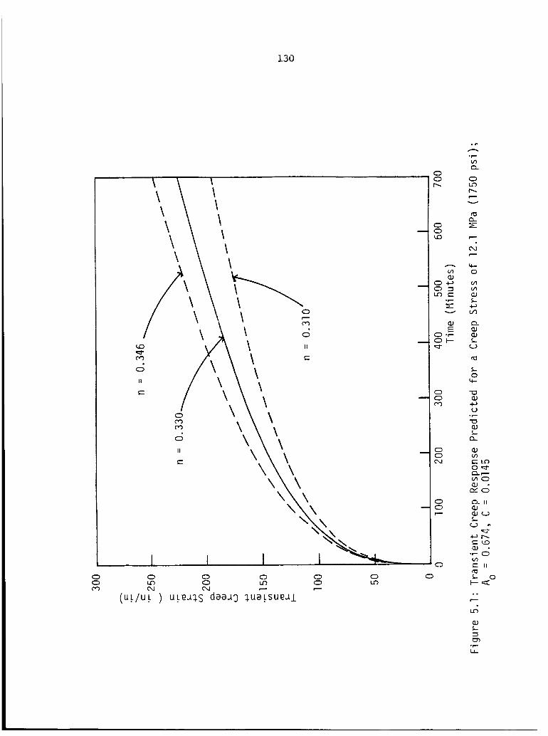
130
0CDo_
\\ ',
0 0 0 0 0
(UL/UL) uLea_S daaa9 _UaLSUeal
00
00
0
_0 c-
or-
0E
OI--
00o')
00O,J
00
0
0
0
v
t_O_
o,J
0
0,10_
0
o")
r_
(D&__._
0q--
(D
0°_
(D
c- LO
_Z. f.-'--
•,-- o
M
S,-
°r,-Is_
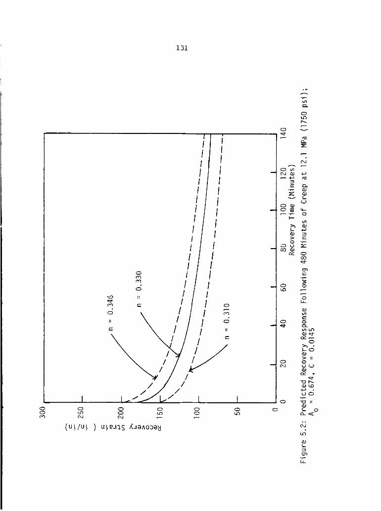
131
C9CDCO
'/III
IIIII
III
II
C) _ 0 _
(u.t/u.t) u.tEa:_S ,_aa^0_a_
iIIIIIIIII
II
I0 _
o_
°_,_(._
0
P_
0 v
rt_r_
°r"- I_
v _
V1
Q .r--
a9 _
.r--
0 0
l..U.
C-
¢'_ r'-
C,.l U_J
o_.,.
M
(D
.,_-.LI_

132
described above, a 480 minute/120
recovery test cycle was selected.
minute creep/creep
Proposed Test Selection Process
The procedures followed in selecting the creep/creep
recovery test schedule were intended to assure accurate
long-term prediction of viscoelastic response. The test
selected depends to a certain extent upon the material being
studied, in the present case T300/5208 graphite-epoxy. It
is likely that a different test schedule would be selected
if a different material were being investigated. Therefore,
the test selection process followed during this study has
been itemized below. This "standard" procedure would serve
to address those variables which are essential for accurate
long-term predictions.
• Obtain initial estimates for the linear viscoelastic
parameters A o, C, and n through a few relatively short
creep/creep recovery tests at low stress levels.
• Determine the desired maximum time of prediction and
desired accuracy at the maximum time. In the present
study these were 105 minutes and !I0%, respectively.
• Using the initial estimates for A o, C, and n, calculate
the expected "exact" response at the maximum time of
prediction (using eq. 5.1) and the acceptable error
bounds in predicted creep strain at that time.
• Calculate the acceptable error bounds for the power law
exponent n (using eq. 5.2).
• Determine the "confidence" level for the strain
measuring system being used. In the present study,
this confidence level was specified as +20 _in/in.
133
• Determine the creep time required to distinguish thecreep response for an n value outside of the acceptablerange in n. In the present study, this creep time wasdetermined to be 480 minutes, using Figure 5.1.
• Select a recovery period based upon the expectedrecovery response after the creep time determinedabove. In the present study, the recovery periodselected was 120 minutes, based upon Figure 5.2.
These general guidelines should be especially helpful to
the researcher studying a viscoelastic material which has
not been previously investigated.
VI. ACCELERATED CHARACTERIZATION OF T300/5208
During this study, the accelerated characterization
scheme described in previous chapters was applied to the
T300/5208 graphite-epoxy material system. The viscoelastic
response of unidirectional 90-deg and 10-deg off-axis
specimens was monitored during 480 minute/120 minute
creep/creep recovery tests, conducted at several stress
levels. These tests were used to characterize the
viscoelastic behaviour of the matrix-dominated properties
$22 and $66. A few tests were conducted using O-deg
specimens to measure the fiber-dominated properties SII and
S12. Specific details including specimen fabrication,
equipment used, data collection techniques, typical data
obtained, data analysis techniques, and results of the
short-term analysis will be presented in this chapter.
Specimen Fabrication
Specimens were fabricated from 8-ply panels of
T300/5208. These panels were layed up by hand, using NARMCO
RIGIDITE 5208 Carbon Fiber Prepreg tape with a fiber volume
fraction of 65_. It is desirable to cure composites in an
autoclave, since the resulting composite laminates are
generally of a higher quality than those produced by other
methods. However, the use of an autoclave could not be
134
135
arranged within the time frame of the present study, and
therefore the panels were cured using the VPI&SU hot press
facility. The heat and pressure cycle used to cure the
panels consisted of the following steps:
• Initial heatup from room temperatures to 135C (275F),at an average rate of 2.8C/min (5F/min), at atmosphericpressure
• Hold temperature at 135C for 30 minutes at atmosphericpressure
• Apply 6.89 kPag (i00 psig) with platens
• Raise temperature to 179C (355F) at 6.89 kPag and holdfor 120 minutes
• Cool in press to 60C (14OF) at 6.89 kPag
• Remove from press and air-cool to room temperature
Nominal panel dimenslons were 0.i0 cm X 30.5 cm X 30.5 cm
(0.04 in X 12.0 in X 12.0 in).
A problem experienced throughout the program was a
shortage of prepreg tape. The experimental portion of the
program was initiated using prepreg on hand, which had a
fiber volume fraction of 65_. After a significant amount of
testing had been completed, it was learned that additional
prepreg with the same fiber volume fraction was not
available. Rather than repeating all of the tests which had
been conducted up until that time, the program was continued
using the limited amount of materials on hand. This caused
some difficulty with respect to selection of the laminates
used during the long-term creep studies. These problems
136
will be further discussed in Chapter VII.
The tensile specimens were sawed from the panels using a
diamond wheel abrasive disk. Nominal specimen width was 1.3
cm (0.50 inch). Specimen length ranged from 17.8 cm to 33.0
cm (7.0 to 13.0 inches).
It has been shown [20-22,39] that previous thermal
history can dramatically affect the viscoelastic behaviour
of polymer-based composite materials. Therefore, after
being sawed from the panels, all specimens were subjected to
a post-cure thermal treatment. This treatment was intended
to erase the influence of any previous thermal histories,
and to bring all specimens to a common thermodynamic (i.e.,
viscoelastic) reference state. The post-cure consisted of
the following steps:
• Initial heatup from room temperatures to 177C (350F) atan average rate of 2°6C/min (4.7F/min)
• Hold temperature at 177C for four hours
• Cooldown from 177C to approximately _9C (12OF) at aclosely controlled rate of 2.SC/hr (5F/hr)
• Remove from oven and air-cool to room temperature
After post-cure, all specimens were placed in a desiccator
at a relative humidity of 21% _ 3% until used in testing.
Specimens were strain gaged using gages mounted back-to-
back and wired in series, as described by Griffith, et al
[20]. Using back-to-back gages in series serves two
purposes. First, the effective resistance of the strain gage
137
is doubled, which allows the use of a relatively high
excitation voltage resulting in high sensitivity, while
still maintaining low gage current and good gage stability.
Secondly, any effects due to specimen bending are
electrically averaged and therefore removed from the strain
gage signal. Micro-Measurement 350_ WK-series strain
gages were used. The WK gage alloy is especially stable and
suited for use at high temperatures [54]. The gages were
mounted to the specimens using the M-BQnd 600 adhesive
system. This is an elevated-temperature adhesive requiring
a cure temperature ranging from about 75C (175F) for 4 hours
to about 175C (350F) for 1 hour [55]. In the present study,
a cure at 82C (18OF) for 8 hours was used to assure complete
cure of the adhesive while still avoiding any perturbation
of the post-cure thermal treatment.
For 0-deg and 90-deg tensile specimens, uniaxial strain
gages were mounted along the major axis of the specimen,
parallel to the load direction. For lO-deg off-axis
specimens, a 3-element strain gage rosette was used,
oriented as shown in Figure 6.1. All gages were mounted
using a magnifying glass to aid in gage alignment.
Since WK-series gages are provided with preattached
leadwire ribbons, lead wires were soldered to the ribbons
rather than directly to the gage tabs. This avoided placing
the soldering iron tip in direct contact with the specimen,
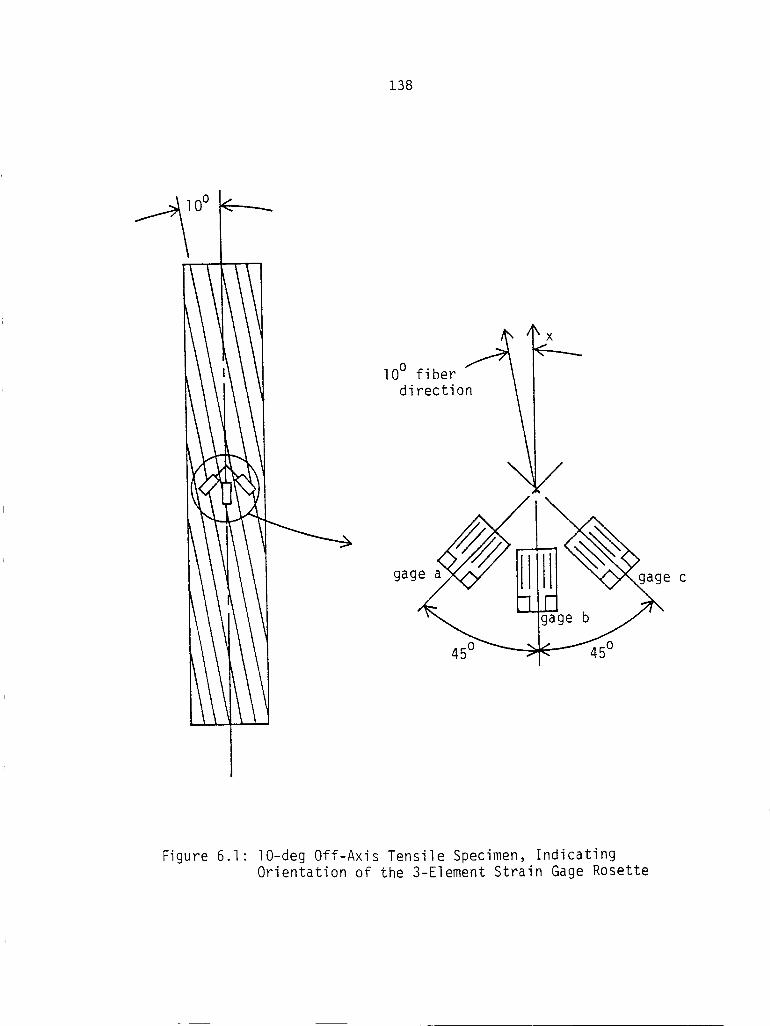
138
<--__._
I\\I
///,!!\!
N_.,.. s Sl
l i v
\/\i i i ,
I0 ° fiber fl
directi°n /
\
gag
45o"---..._
\x
/
e c
Figure 6.1: lO-deg Off-Axis Tensile Specimen, IndicatingOrientation of the 3-Element Strain Gage Rosette
139
which can cause local damage in the form of broken fibers,
damaged epoxy matrix, or both [56]. Micro-Measurements
330-FTE leadwire was used, which is a 3-conductor, stranded
silver-plated copper wire with Teflon insulation, suitable
for use to 260C (500F).
Thermal compensation of the strain gage signal was
accomplished using the dummy gage technique [57]. In this
method, a gaged "dummy" specimen is placed immediately
adjacent to the mechanically-loaded "active" specimen. In
all cases, the dummy specimen was identical to the active
specimen with respect to gage type and gage/fiber
orientation. The two specimens were wired in adjacent arms
of a Wheatstone bridqe circuit. Ideally, the dummy specimen
experiences the same thermal history as the active specimen.
Due to the characteristics of the Wheatstone bridge circuit,
any gage response to temperature is cancelled and the
remaining gage signal is entirely due to the mechanical
load.
Equipment Used
Tensile creep loads were applied using one of three
different dead-weight creep frames. All frames utilize a
lever-arm system to apply the tensile creep load. The
majority of the short-term creep/creep recovery tests were
conducted using an Applied Test Systems (ATS) creep machine
140
either ratio
equipped with an ATS
temperature controller.
within +I.IC (!2.0F).
featuring an automatic loading system and load re-leveler.
The lever arm for this frame is adjustable to either a 3:1
or I0:i load ratio. The maximum applied load capacity at
is 88,964 N (20,000 ibf). The frame is
series 2912 oven and series 230
Oven temperatures are maintained to
A few short-term tests were conducted using a Budd creep
frame, also equipped with a ATS series 2912 oven and series
230 temperature controller. The load ratio for this machine
is fixed at i0:I. The maximum rated load for this frame is
26,690 N (6000 Ibf). This frame was used infrequently and
only when the ATS machine was not available.
The long-term laminate creep tests were performed using
a five-station creep frame. This frame was designed and
built in-house during the present study, specifically for
the long-term creep tests. The supporting structure of this
frame is a channel- and I-beam weldment, produced in the
VPI&SU University Machine Shop. Tool steel, surface treated
to a hardness of R 58-60, was used for all knive edges andc
mating surfaces to reduce the effects of plastic deformation
and friction. Each of the five lever arms has a fixed load
ratio of I0:i, and were designed to apply a maximum load of
13,345 N (3000 lbf) per arm. (Perhaps it should be noted for
further reference that no loads greater than 4448 N were
141
applied during the present study.) Five individually
controlled ovens were constructed using sheet steel and
aluminum angles, and were insulated with a 2.5 cm (I.0 inch)
thickness of Carborundum FIBERFAX ceramic insulation. The
interior cavity of each oven is nominally 15.2 cm X 15.2 cm
X 53.3 cm (6.0 in X 6.0 in X 21.0 in). Heat is introduced
using Watlow resistance heating elements and controlled
using Omega model D921 digital temperature controllers.
Temperatures were maintained to within !l.lC (!2.0F) over
the 105 minute creep period.
Strains were measured using either a Vishay series 2100
amplifier and strain gage conditioning unit with MTS model
408 voltmeter (used with either the ATS or Budd creep
frames), or with a Vishay P-350A portable digital strain
indicator with SB-IK ten-channel switch and balance unit
(used with the five-station creep frame). Strain and time
data pairs were logged by hand and subsequently entered into
the IBM mainframe, housed at the VPI&SU Computing Center.
All further data reduction was accomplished using the IBM
mainframe and FORTRAN programs. Strain data were taken with
an amplifier gage factor setting of 2.0, and were
subsequently corrected for actual gage factor and (where
appropriate) for transverse sensitivity effects.
142
Selection of Test Temperature
As previously noted, the Schapery theory can be
considered to be a Time-Stress Superposition Principle. A
viscoelastic material can therefore be characterized at a
single temperature through a series of creep/creep recovery
tests at several stress levels.
Time-Temperature Superposition
material may be characterized
This is in contrast to the
Principle, in which a
at a single reference
temperature through a series of creep tests at a common
stress level but at several temperatures. Temperature-
dependence was not considered in the present study, and all
tests were conducted at a single test temperature.
Dramatic viscoelastic response was desired so as to
provide a rigorous check of both the Schapery theory and of
the laminate characterization scheme as a whole. Therefore,
a test temperature approaching the T of the epoxy matrixg
was required. The T was determined through a series of 5g
minute creep tests at temperatures ranging from 66C (150F)
to 199C (390F). A 90-deg unidirectional specimen was used
at the relatively low stress level of 11.4 MPa (1650 psi) to
assure a linearly viscoelastic response. The creep strains
at 1 and 5 minutes were recorded, and an "average creep
rate" was defined as
AE _(t) --E(1)At 4

143
Both the 5 minute creep compliance and the average creep
rate have been plotted as functions of temperature in Figure
6.2. As indicated, the 5 minute creep compliance
measurements indicated gave a T of 178C (353F), whileg
average creep rate measurements indicated a Tg of 180C
(356F). This mild discrepancy was considered to be within
experimental error bounds. These results are also in
agreement with results presented elsewhere [II].
A test temperature of 149C (300F) was selected, based
upon Figure 6.2. It was reasoned that adequate viscoelastic
response would occur at this temperature, without severely
reducing specimen strength or rigidity.
Tests of 0-deg Specimens
Two tensile tests were conducted using 0-deg specimens
to determine the fiber-dominated properties Ell and v12 (or
equivalently, SII and S12 ). These properties were assumed
equal in tension and compression. As expected from previous
results [11,18-23], neither Ell nor v12 exhibited
appreciable time-dependent behaviour at a temperature of
149C, and were therefore treated as linear elastic
properties during the laminate analysis. The results
obtained and used in the analysis were
= 132.2 GPa (19.16 X 10⁶ psi)Ell
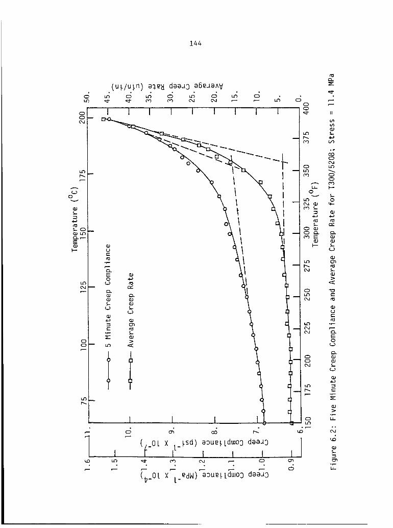
144
LO
CD0 --
¢,4
LO
c_)0v
4_
_-CD__
C_. r--
E
LO(xJ--
oo_
r'_
7_0
I ! I I I I I I 1
I
I
II
c_
(./3
°_
0
t._
0C)
I--
S-0
W-
t_
O._J
(D
>
"0c-
Q.)
t_
00
O.
.t-
>._,.-L:_
Od
145
or,
= 0. 273v12
i
SII = E11= 7.570 x 10 -12 GPa -I (52.19 x 10 -9 psi -1 )
-v12
S12 = E2110 -12--= - 2.067 x GPa -I (-14.25 x 10 -9 psi -1 )
The tensile modulus value can be compared to the results of
Kibler; Ell = 136 GPa [II].
Tests of 90-de_ Specimens
The 90-deg tests were used to characterize the
viscoelastic response of the matrix-dominated modulus E22.
The ultimate strength perpendicular to the fibers at 149C
was inititally estimated to be 31.1 MPa (4500 psi), based
upon a parallel study by Zhang [58]. This ultimate strength
was somewhat lower than expected. Sendeckyj et al [59]
report an ultimate strength of 49.6 MPa (7160 psi) at room
temperatures for T300/5208. Therefore, an ultimate strength
of perhaps 41.4 MPa (6000 psi) had been anticipated at a
temperature of 149C. However, during the present study even
the lower strength levels observed by Zhang were not
attained, as all 90-deg specimens failed at stress levels
greater than 20.7 MPa (3000 psi). This failure occurred for
146
a total of four specimens, two of which had been used in
previous tests and two of which were virgin specimens. All
failures occurred in the specimen grips rather than in the
strain gage area. These specimens were rather delicate, and
it is possible that they were damaged slightly during gaging
and/or mounting in the grips, although care was taken to be
gentle. Further tests with new specimens were not possible
due to the material shortages mentioned above. It should be
noted that in previous viscoelastic studies at VPI&SU 16-ply
specimens were used rather than 8-ply specimens. Perhaps in
future efforts 16-ply specimens should again be used, since
the increased specimen
durability.
Strain data for
thickness may help to improve
the entire 480 min/120 min
creep/recovery test cycle were obtained at seven stress
levels ranging from 10.5 to 20.7 MPa (1528 to 2997 psi).
For each test, a minimum of 26 creep and 21 recovery data
points were taken, at the nominal times listed in Table 6.1.
Following collection, the data were entered into the IBM
mainframe computer and reduced using either the SCHAPERYor
FINDLEY programs described in Chapter III. An interactive
graphics routine was also written which allowed an immediate
plot of the data and analytic fit. Sample plots are shown
in Figures 6.3-6.5. The entire creep/recovery data set is
shown in Figure 6.3. The solid line represents the analytic

147
Table 6.1: Nominal Measurement Times For The 480/120 MinuteCreep/Creep Recovery Tests
Creep Measurement TimeNumber Time (minutes)
Recovery Measurement TimeNumber Time (minutes)
1 0.5 1 O.2 1.0 2 O.3 1.5 3 O.4 2.0 4 I.5 3.0 5 I.6 4,0 6 2.7 5.0 7 3.8 7.0 8 4.9 I0. 9 5.
I0 15. I0 7.II 20. II I0.12 25. 12 15.13 30. 13 20.14 40. 14 25.15 50. 15 30.16 60. 16 40.17 90. 17 50.18 120. 18 60.19 150. 19 80.20 180. 20 I00.21 210. 21 120.22 240.23 300.24 360.25 420.26 480.
255O750500000

148
I I I
6 6 6O O OO (D _0
I I I I I
5 6o o o 6 6 6 6
( NI/NIO_DIW ) NIU_±S
OO
OLDtO
OOCD
OLDLf#
LD
I--o -n
_ z
S z
i,io 5-
I--
0
m
OLDN
oO¢J
OLD
OO
d
O_OCD
mI--
O_0
0O4
0,l
ZI.d
UL,JnU'}
03(:3
I.,13
00£rjI--
I--'
¢,,_
"F_
0
4._°r-I.I,,.
%¢-
&)o'3
t'O
>._S.-
0U
t-
_- 0
U_.) ._-
C_.
E
0 0
L
O_CO _"
°r,-LL

149
6N
( NI/NIOM31W ) NI_IS d33_ 1N31SNW_I
<51.0
(5O1.0
W
('_ i,=4
w
N
O-tO
b.OOm,I--
LOO.0c,40(N
co
zw
uWO.LO
¢oo
u_
0o(7oI-
°_
L
4-J
¢.-
¢.-4J
c-
O.).4-)
0
_7°_
U°r--
f-.
¢..-
¢-
0(D ,"_"
E U• 1" .P"
¢:L0 r_O0 _-
°p-
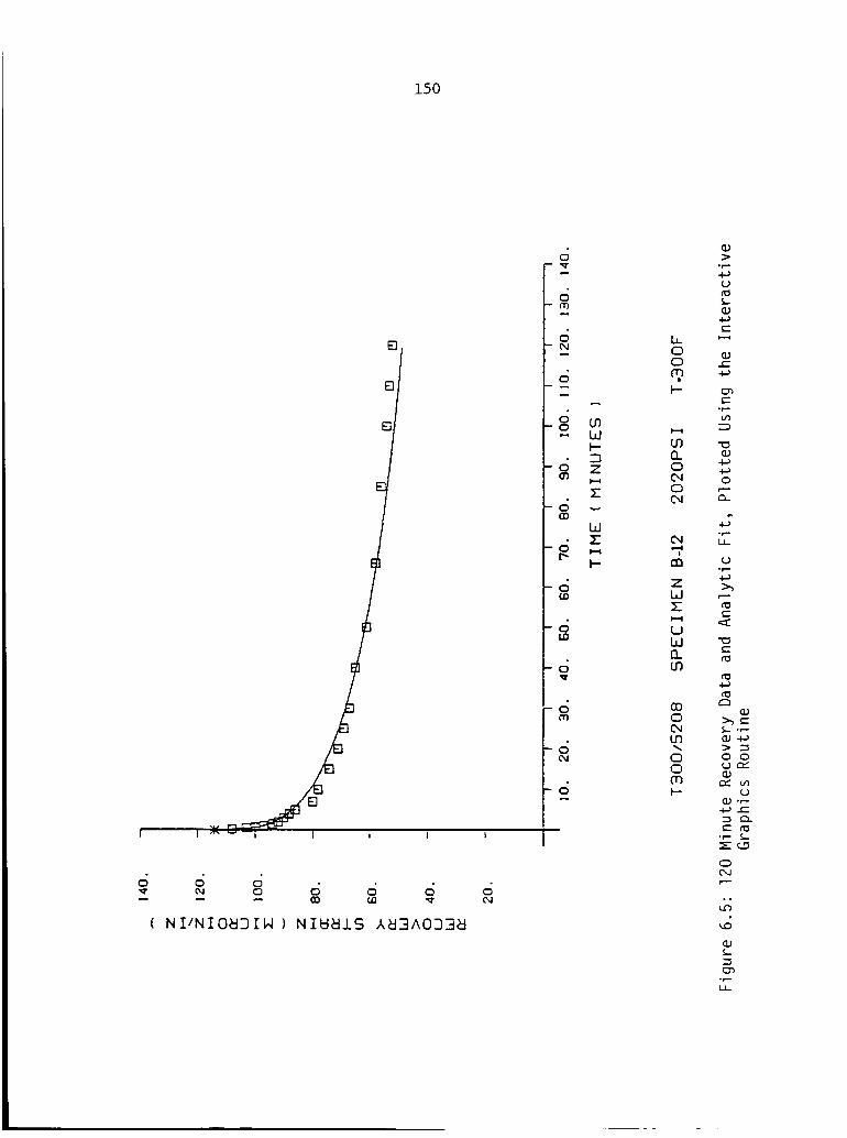
150
E]
E]
I I I
6 6 6N o 6 d 6 6
( NI/NIO_DIN ) NIW_±S _,_-4A0O3_d
6
600
66,1
6
o
O
O(D
"-O1.0
--O
--O00
--O
--O
tOWH-
Z
W5-
L00
m.p-
U3O.0O40O4
O4
t_
ZW
UW8_tO
¢00
C)0O3I--
°r--
Z)
0
t'_
°r-'-
°r-
%c"
t_
.f,-
0 0(Dew"
(D
_"QD
0
._.,.
151
fit provided by the SCHAPERY program. The transient creep
response is shown in Figure 6.4; i.e., the instantaneous
response has been subtracted from the creep data and only
the transient viscoelastic response is shown. Recovery data
and analytic fit are shown in Figure 6.5. This plotting
routine was used to detect any input errors and as a visual
check of the analytic curve fit.
One difficulty associated with the relatively long 480
minute creep period used in this study was the resulting
long time required for specimen recovery. At the lower
stress levels, the recovery response was complete after a
1-2 day period, and a new test could be initiated. At the
higher stress levels, a considerably longer recovery time
was neccessary; at the highest stress levels a recovery
period of i0 days was required. Also, at these higher
stress levels, a permanent non-recoverable strain was
recorded. The permanent strain following recovery will be
further discussed below. In these cases, recovery was
judged "complete" when the strain measurement did not change
appreciably over a 24 hour period.
Stress-strain curves obtained at 0.5 and 480 minutes
during the creep cycle are shown in Figure 6.6. Results
indicate very slight nonlinear behaviour at stress levels
greater than about 15.6 MPa (2250 psi). This result was not
unexpected, since slight nonlinear behaviour for 90-deg
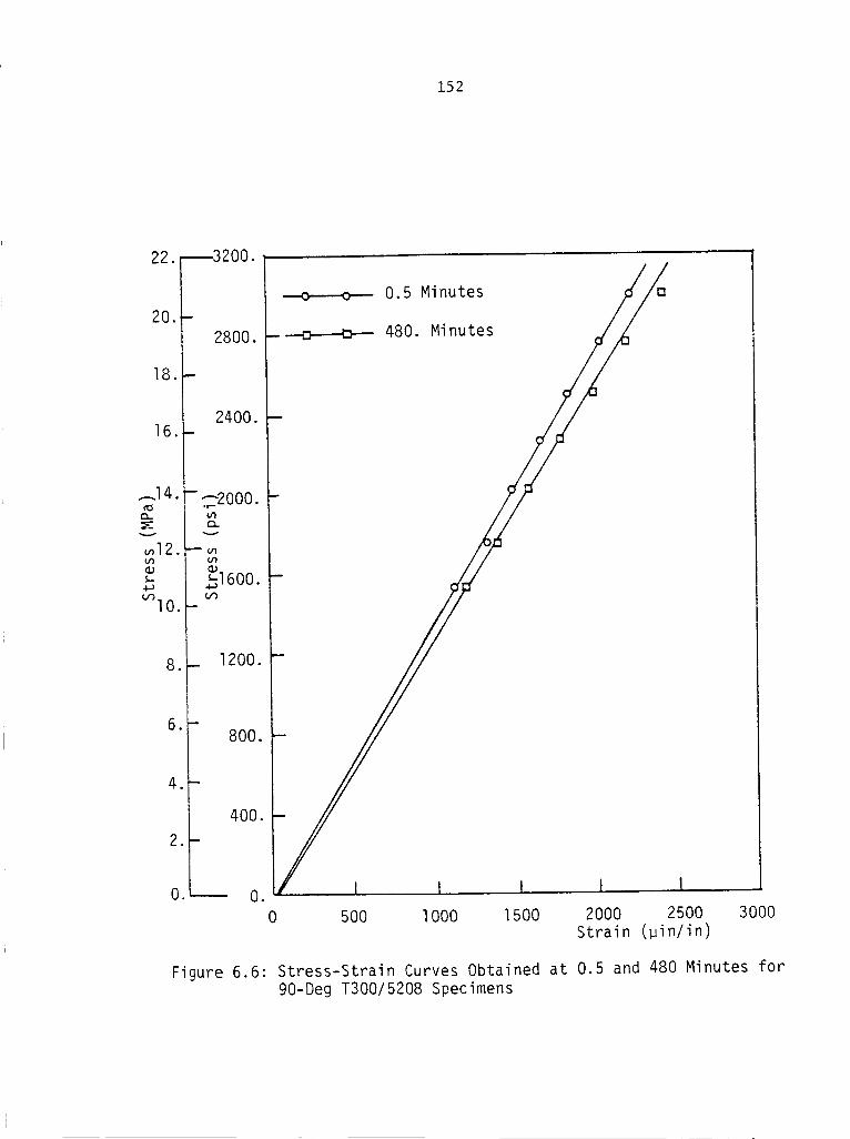
152
22"I--3200"20.
18.
16.
.-.I 4.¢0
r_
v
_12.
_I0.
a
q
,
1
2800.
0.5 Minutes
480. Minutes
2400.
i
2ooo.
_1600.
_ 1200.
800.
400.
I
0.-- O. I ,I
0 500 1000 1500 2000 2500 3000Strain (pin/in)
Figure 6.6: Stress-Strain Curves Obtained at 0.5 and 480 Minutes for90-Deg T300/5208 Specimens

153
specimens of T300/934 had been suspected by Hiel [22],
although the creep/creep recovery cycle he used was not long
enough to distinguish nonlinear behaviour. The results
presented in Figure 6.6 confirm this suspicion and also
raise an interesting question regarding the concept of a
linear/nonlinear distinction in stress level. That is,
while the results obtained at 0.5 minutes indicate linear
behaviour at any stress level, the results obtained at 480
minutes indicate nonlinear behaviour at stress levels
greater than 15.6 MPa. It can be hypothesized that if creep
data had been taken at times greater than 480 minutes
nonlinear behaviour would have been evident at stresses
lower than 15.6 MPa. Therefore, it may be that nonlinear
behaviour occurs at any stress level for T300/5208, but is
not apparent at short times for low stress levels.
From a practical viewpoint, if viscoelastic behaviour is
to be predicted at time t = 0.5 minutes, then nonlinear
effects can be neglected at any stress level. Conversely, if
the prediction is to be made for 480 minutes, then nonlinear
behaviour must be accounted for at stress levels greater
than 15.6 MPa. Thus, the decision as to whether to include
nonlinear effects in an analysis depends upon the desired
length of prediction. This greatly complicates the process
of accelerated characterization, since it implies that
nonlinear effects important at long times cannot be sensed

154
with sufficient accuracy at short times. A possible
solution would be to couple the TSSP (i.e., the Schapery
model) with the TTSP, or in other words accelerate the time
scale using both stress and temperature. This approach was
not used in the present study, but is worthy of further
consideration. For this study it was decided to treat data
obtained at stress levels less than or equal to 15.6 MPa as
linear data, and treat data obtained at the higher stress
levels as nonlinear data.
Another factor which complicated the analysis was that
complete recovery was not observed following each test,
indicating an accumulation of damage within the test
specimen. The permanent non-recoverable strains recorded
for the 90-deg specimen are shown in Figure 6.7. As
previously discussed this problem was also encountered by
Hiel [22], and was treated as an offset error in the
recovery data. In the present case the effects of permanent
strain were investigated by comparing the results of five
separate analyses. The linear viscoelastic parameters Ao,
C, and n were first determined using the linear creep data
and the FINDLEY program. Recall that the sensitivity
analysis presented in Chapter IV indicates this to be the
best approach for calculating the power law exponent n.
Next, Ao, C, and n were determined using the SCHAPERY
program and linear creep and uncorrected recovery data. That

155
¢,4
E_. ¢,J
v
o0
COCO
m
0
-I0
Od
0
0
0
I I I I0 0 0 0
(ULIULd) u£eJ_S _ueuewaBd
0
0
I0
0
c,')
N
0
__ 1.0C',,l
0-- 0
0C_
0
( 0-- 0
0
C,dC) ,--
000
0
p_ c_
4-_
>0
c-"°_
0OJ
0CO
0'_E
or- •_g
0
0
O0
_h"-
m _
• r- |
4-_
c"
_ m(1.1_
_ mE4--_
_.- I---
P_
G
0r,,
LJ-
156
is, the accumulated damage was not accounted for in this
second analysis and the recovery data used contained an
"offset error". This analysis is included to illustrate the
detrimental effects of such errors on the viscoelastic
analysis. In the third and fourth analyses attempts were
made to account for the accumulated damage within the linear
recovery data. Two approaches were used, which will be
referred to as "Method I" and "Method 2". Finally, the
remaining nonlinear parameters go' gl' g2' and a c were
determined using nonlinear data and the SCHAPERY program.
Analysis Using Creep Data
In this section, the results obtained using the program
FINDLEY will be presented. The creep data used were
obtained at stress levels of 10.5, 12.1, 13.9, and 15.6 MPa
(1528, 1748, 2020, and 2263 psi). Note that the creep data
was not corrected for any permanent strain error. The
values obtained for A o, C, and n are shown in Figure 6.8.
The average value and standard deviation for each parameter
were
A = 0.1.062 + 0.00037 ( X I/GPa)o
= 0.7321 t 0.00252 ( X lO-6/psi)
C = 0.00136 Z 0.00016 ( X I/GPa-min n)
= 0.009372 + 0.00111 ( X 10-6/psi-min n)
n = 0.289 + 0.0158

157
v
OJm
m
0m
0
i
0anL_A V
,.-- _
[]
0
> >0
> > >< < ,=_
II
0
0
o D
ItOo'3
''o '
0
Q
0 Q
I I0 _
anl_A u
I,4
4
I0N
,=S
I
0
,:::;
I I I IN 0 CO _0,.-- ,.-- 0 00 0 0 0
_nLeA O
0
NN
EcOc_
0
0-
0"}
o U
m _
_ E
4-_ e._
(1)0U
f,.-
(2;
0-- 0
L_
0uON
l00
c_
.t--
...J
-g=
0_.-
"_
.g
mLs.J
(lJ .-J
/d
158
Recall that all three of these values are expected to remain
constant with stress. Based upon the analysis presented in
Chapter V, it was hoped that the test cycle selected would
result in an accuracy in n ranging from -6.1% to +4.8% of
the actual value. The standard deviation will be used as an
indication of accuracy; thus possible experimental error in
the value obtained for n is +5.5%. Therefore, the expected
accuracy in n was not quite attained. Admittedly, neither
the number of tests nor the number of stress levels used are
of a statistically valid sample size. Nevertheless, these
results exhibit considerably less scatter than those
obtained using a different creep cycle [21]. The possible
error in C (shown in Chapter IV to be less important than
errors in n) is 111.8%, while the possible error in A ° is
+0.3%.
Analysis With Uncorrected Recovery Data
The Ao, C, and n values obtained using the SCHAPERY
program and uncorrected recovery data are shown in Figure
6.9. As indicated a very wide scatter in both C and n was
encountered. This would be expected based upon the analysis
described in Chapter IV, since the recovery data contains a
large offset error due to accumulated damage. The average
value and standard deviation for each parameter are

v
¢0i/1 r-.-
l/1
1-4_O0
I
0
r..- ¸
_O
tl_ tO
¢xJ --
m/..-
0 __e--
0
t.--
I
an L_A °V0'_
159
CO r--
C5
0
0 0 0
tO tl_%. _ t.0 _lJ CD
0
t'-I ¢-_0
o []
I 10 _'_
cO
6
I Ic,J 0
0 0
IIIIIII
II
IIIII1IIiIi °IIIII
iI
u 4
'1 °0 co 0 ¢xJ
an lea u
I1 I I I
0 0 0 00 0 0 0
an LeA 3
0
O,l
0000,1 ----,
"Ev
m
m
m
0
If)
i-....-
E
i.
0i.
c-4-_
"_,
c-
4._
E
°_-
04-10
09
0
0 0
C" 0• _- ¢'w"
0 0c" 4_
4-_ 0
i. t-
O i-_4-- 0
0
C"
-0
0>"
O_l,I
e----t-
°_...Ll-
160
A ° = 0.1068 ± 0.00048 ( X I/GPa)
-6/psi= 0.7363 Z 0.00328 ( X I0 )
C = 0.000986 ± 0.000286 ( X i/GPa-min n)
= 0.006816 ± 0.001970 ( X 10-6/psi-min n
n = 0.342 + 0.0527
The possible error in n and C are therefore _15.4% and
+28.9_, respectively. Note that the estimate for A-- o
obtained using either FINDLEY or SCHAPERY is essentially
equivalent, since in both cases A is determined using theo
creep data.
Analysis With Recovery Data Corrected Usinq Method 1
In this analysis, the accumulated damage recorded
following each test was subtracted from the recovery data.
This approach was used by Hiel [22], and will be referred to
as Method I, to distinguish it from an alternate procedure
described in the next paragraph. The A o, C, and n values
calculated using this approach are presented in Figure 6.10.
The average values and standard deviations are
A ° = 0.1057 _ 0.000398 ( X I/GPa)
-6/psi= 0.7288 ± 0.002746 ( X I0 )
C = 0.001813 Z 0.0004186 ( X I/GPa-min n)
= 0.0125 _ 0.002886 ( X lO-6/psi-min n)
n = 0.257 + 0.0258

161
0 -- _-_,--- _:I
r-_
c-
O
0_,_
C
anl_A °V
i I 1
I
I I
0
o
o
I0
0
0
0 0
0"_ Ont_l t_
0 0
0
a 4
[]
r_
c_
I
IIIIIIIIIIIIII!
I!IiIIII
[]
O,J
,:::;an L_A u
I I I
I
E
0
0 0t_ c-
Od
0o %(M
t_
c_t_ t_
°r'- ¢_._J .,_
,.-- c_ Qj
0_- 0
Q;r_c--
r_O>-
0o I._J
00-0 "_:Z
_(xJ c_ (..)
0 °_"
LID
0 0 0
an L_A O
0
I0
0
,:S

162
The possible error in n and C for this case are _i0.0% and
Z23.1%, respectively. Thus, correcting the recovery data by
Method 1 reduced the scatter in n and C, but not to the
levels obtained by using the creep data.
Analysis With Recovery Data Corrected Using Method 2
Note that since the response is assumed to be linear eq.
3.4 can be used to generate an analytic recovery curve based
upon the creep response. That is, the C and n values
obtained using the creep data (C = 0.009372; n = 0.289) can
be substituted into eq. 3.4 to obtain an expression for the
expected recovery strain at any time t. Based upon this
approach, the recovery curve expected at a stress level of
15.6 MPa is compared with the uncorrected and corrected
recovery data in Figure 6.11. It would appear from this
figure that the difficulty lies in an inaccurate permanent
strain measurement; i.e., the correction used to account for
accumulated damage was too severe, causing the corrected
recovery strains to "overshoot" the expected recovery curve.
Similar calculations indicated an overshoot had occured at
all stress levels. The discrepancy between expected
recovery strains and corrected recovery strains was on the
order of 5-15 _in/in in all cases. While this is a
relatively small error, it has been demonstrated in Chapter

163
oo
0
0
0
0
0
0
0
0
0
0
0
0
0
0
n
0
oco
o o
(u_lu_)
o o o o0,J 0 00 _.o
uLea_S £aeA0na_l
o
Io o
o
o
r.- 0
.r--
0"--_O_
0E
°r"-
oco
o
ooo
o
o
o
o¢'0
oc_J
o
o
t_
t_r-_
o
-_
00t_mm
00
0'3
v_
_- o_- _-
._-
>(.30
tnoX
4--O_
0o9
tO_--
0 c-O
164
IV that errors of this magnitude severly distort the results
obtained using recovery data.
These considerations gave rise to a second approach for
correcting the recovery strain, which was to simply adjust
the measured data so as to match with the expected recovery
response as closely as possible. This is not proposed as a
valid experimental technique, since it requires a priori
knowledge of the recovery response. The intent is rather to
4etermine whether the measured recovery data can be "forced"
to agree with the results obtained from creep. This
procedure will be referred to as Method 2. The optimum
offset shift of the recovery data was determined as follows.
The expected recovery response at each stress level was
calculated and subtracted from the measured strain at each
point in time. The difference was defined as an offset
error for that point in time. The average offset error over
the 120 minute recovery period was then calculated for each
stress level and subtracted from the recovery data as
before. The resulting fit between predicted and corrected
recovery strains is illustrated in Figure 6.12 for a stress
level of 15.6 MPa. Similar results were obtained at all
stress levels. Casual inspection would suggest that a very
good correlation between the C and n values calculated using
creep and corrected recovery data would now be obtained.
However, the correlation did not improve and in fact
165
oo
0
o
0
o
o
o
o
o
o
0
0
0
o00
o o o o o04 o 00
u .tea_S ,QaA03a_l
I Io o o
oJr--
oos-
O
r.- o
o
0 _o o ,'_
E 04°r _
co _- t_ o
o Lr_O_ _-- _
0 >_-)_'_ 0
_-0
',I
0 _-CO 0"_
0
0 _-
0 °°
*r-i,
o
0
166
slightly worsened. The Ao, C, and n values obtained are
presented in Figure 6.13. The average values and standard
deviations are
A ° = 0.1062 ! 0.000786 ( X I/GPa)
= 0.7324 _ 0.00542 ( X 10-6/psi)
C = 0.001426 _ 0.000472 ( X i/GPa-min n)
= 0.00983 ! 0.00326 ( X 10-6/psi-min n)
n = 0.295 + 0.0401
The standard deviations indicate possible errors for n, C,
and A ° of t13.5%, !33.2%, and !0.74%, respectively.
The reasons for this rather suprising result are not
clear, although by careful inspection of Figure 6.12 a
potential explanation is suggested. Note that for times
less than about I0 minutes the corrected recovery data
points lie slightly below the predicted recovery curve,
while at longer times the data points lie slightly above the
predicted curve. This same pattern existed at the other
stress levels. Thus, the experimental data points describe
a slightly "flatter" curve than predicted by linear
viscoelastic theory. This indicates slightly nonlinear
behaviour, which could perhaps explain the erratic results
obtained. Specifically, a flatter recovery curve indicates
that the gl parameter is greater than 1.0, as discussed in
Chapter III. This reasoning also implies that the recovery
167
LO
v
O0
0
I
m
m
_I'
o o
m
I0
0
I
l
0
4
0
I
gnlgA
O
o
0v
kO
c_anIgA u
I0oO
O0
II
III
o D
0 0
I II I
O
I t I I I_O ,m' O J O CO
O O O _ O
an IgA 3
kO
04
O
O ._-
g')u')_J
4_
O
OO
n---
Oko
O,--
c_
kOOO
E
O
_J
c--i,.,-
e-
e-r_
%
S.
¢-_ ¢',4
._--
*r--
(2.1
•_-- _._
0
4-- 00
¢--
._--
,----r-
..
O0
IA.-
168
response is more sensitive to nonlinear effects than is the
creep response, since satisfactory results were obtained
using the creep data and linear theory. This greater
sensitivity to nonlinear effects in the recovery data has
also been observed by Lou and Schapery [35].
Another possible contributing factor would be that the
effects of accumulated damage have not been properly
accounted for. Damage is presumably accumulated through the
formation of voids and/or microcracks which form during the
creep cycle. Such imperfections may occur immediately upon
loading, or may develop gradually during the creep cycle.
In this second case the shape of the creep curve may be
altered due to damage accumulation, ultimately affecting the
calculated values of C and n. Upon unloading, these voids
and microcracks would tend to close and perhaps modify the
shape of the recovery curve as well. The creep/creep
recovery response would therefore depend upon some
combination of viscoelastic, plastic, and fracture
mechanisms. Erratic results may have been obtained because
the Schapery theory does not account for these hypothesized
plastic or fracture mechanisms.
At the least, the above calculations indicate the
extreme sensitivity of n and C to slight errors in the
recovery strain data. This sensitivity tends to confirm the
analysis presented in Chapter IV, where it was concluded
169
that stable values for Ao, C and n can best be obtained
using creep rather than recovery data.
Calculation of the Nonlinear Parameters
The final step in the characterization process was to
calculate the nonlinearizing parameters gO' gl' g2' and a c
at stress levels greater than 15.6 MPa. Specifically, these
parameters were calculated at stress levels of 17.2, 19.0,
and 20.7 MPa (2498, 2755, and 2997 psi). A permanent strain
following recovery was also recorded at these stress levels,
so it was neccessary to correct for accumulated damage by
subtracting the permanent strain from the recovery data
(Method I). Note that since the response was nonlinear it
was not possible to calculate an expected recovery response
based solely upon the creep response, and hence it was not
possible to use Method 2 of the previous section to analyze
the data.
The SCHAPERY program was used to obtain best-fit values
for each parameter. The results obtained for go and gl are
presented in Figure 6.1_, as functions of both the applied
normal stress and of the average matrix octahedral shear
(The average matrix octahedral shear stressstress, _oct"
was discussed in Chapter III.) The go value was calculated
as 1.0 at all stress levels. This implies that the elastic
instantaneous response was linear at all stress levels and
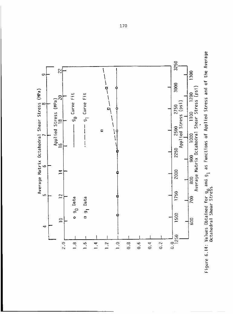
170
Oh
e_
v
u_CO"
S.-
L
LD0
X
eO
t_
' I
_ °r,-
i
r.-
I
O
__ IC CO
£ ,--
.Tin
IIII0
D
I
\
°/
[] 1
I
0
r,m
t_
oO
-- 0 c-
q-0 00 --'-0 • "t_
m__ 0 "_u% ,--- 5- Q.__J ,--- no .,-
00"% c,_
0
-- 0 X.r-.
0
¢0 _-
c_0
00
0;--
0
0°_I
c--
g
._,,.
I..i._
171
that the nonlinear behaviour previously noted in Figure 6.6
was due entirely to the viscoelastic response. The gl
values were somewhat erratic; a value of 1.278 was obtained
at an applied stress level of 17.2 MPa, while values of 1.14
and 1.17 were obtained at stress levels of 19.0 and 20.7
MPa, respectively. The results of Hiel for T300/934
indicate that gl is a gently increasing function of stress
[22], so it was assumed that the gl value obtained at 17.2
MPa was in error and was not used in the analysis.
Recall that an expression for gl as a function of _oct
was required in the lamination program VISLAP. Peretz and
Weitzman [50] have characterized the gl parameter for the
structural adhesive FM-73 using an expression of the form
folS2Io = sI [o0j01" ) !.v
where S I, $2, and o° are material constants determined
experimentally. However, since FM-73 is a highly nonlinear
material, the gl values obtained by Peretz and Weitzman span
a much wider range than in the present case, and the above
expression was not considered compatible with the mildly
nonlinear behaviour observed for T300/5208. Therefore the
following simple bilinear relation was used
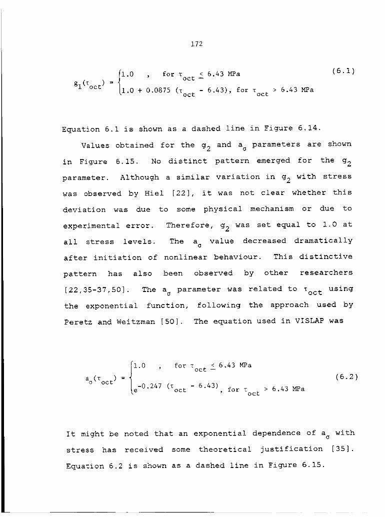
172
< 6.43 MPagl(Toct) = 1.0 , for roct --
1.0 + 0.0875 (r - 6.43), for Toct oct > 6.43 MPa
(6.1)
Equation 6.1 is shown as a dashed line in Figure 6.14.
Values obtained for the g2 and ao parameters are shown
in Figure 6.15. No distinct pattern emerged for the g2
parameter. Although a similar variation in g2 with stress
was observed by Hiel [22], it was not clear whether this
deviation was due to some physical mechanism or due to
experimental error. Therefore, g2 was set equal to 1.0 at
all stress levels. The a ° value decreased dramatically
after initiation of nonlinear behaviour. This distinctive
pattern has also been observed by other researchers
[22,35-37,50]. The a ° parameter was related to _oct using
the exponential function, following the approach used by
Peretz and Weitzman [50]. The equation used in VISLAP was
i , < 6.43 MPa
"i.0 for Toc t _
ao(T°ct) = -0 247 - 6.43)e " (Toct , for T
oct> 6.43 MPa
(6.2)
It might be noted that an exponential dependence of a withc
stress has received some theoretical justification [35].
Equation 6.2 is shown as a dashed line in Figure 6.15.
173
$-
1.0
¢-_0
%$_
4.a
0
x0r-
_J
t.O
_ ¢',J¢,a
n_
_-¢,j
4-_
O3"_r--_J
r.--"
r..'-
0f--
_J
0
4-a
I
III
r_
I I I I
_-- r..- f'-- r--
sanL_A
I
II
o _/
//
o /mII/
=I/I
I ! I I
1.0
0
_0
_J
¢J
0 _0¢-¢0 ,'-,4...)
_0
_J"O
04-a_O_¢,,] _0
e'4.a_o0
0000
_-0d-_-r-
e_4-a
0
e-
_ 0
o_=- _
m XOJ 0r,-
d4

174
Tests of 10-deg Specimens
The 10-deg tests were performed to characterize the
viscoelastic response of T300/5208 to shear stress.
Creep/creep recovery tests were performed at eleven shear
stress levels ranging from 2.9 to 32.5 MPa (426 to 4715
psi). It is well known that end constraints can severely
distort the desired uniaxial stress field when testing off-
axis tensile specimens, particularily near the specimen
grips [60]. Therefore, the 10-deg specimens were 30 cm (12
inches) in length, resulting in a grip-to-grip distance of
approximately 23 cm (9.0 inches). The effective length-to-
width ratio was thus 18, which is considered adequate for
tensile testing. The 480/120 minute creep/creep recovery
test cycle was again utilized, and strain data were recorded
at the nominal times previously listed in Table 6.1. A
3-element strain gage rosette was used to measure three
independent normal strains. The rosette orientation has
been noted in Figure 6.1. For the rosette/fiber orientation
used, the shear strain _12 along the 10-deg fiber direction
can be calculated using the strains measured by gages a, b,
and c as
r12 = -0.598 _a - 0.684 _b + 1.282 _c
175
Note that a different relationship is obtained if an
alternate fiber angle or an alternate rosette/fiber
orientation is used [22,47]. The shear stress _12 along the
fiber direction is related to the applied normal stress oxby
_12 = -0.171 ox
It was found that for an applied tensile normal stress,
gages a and b measured tensile (positive) strains, while
gage c measured compressive (negative) strains. Thus, both
[12 and _12 were negative; for simplicity the results
obtained will be presented herein as positive values.
Stress-strain curves obtained at 0.5 and 480 minutes
during the creep cycle are presented in Figure 6.16. A
comparison of Figs. 6.6 and 6.16 indicates that nonlinear
effects were much more significant in the case of shear
stress than for the case of normal stress. Apparent linear
behaviour with shear was exhibited at the lowest three
stress levels of 2.9, 6.1, and 8.8 MPa (426, 878, and 1279
psi), while nonlinear behaviour was observed at higher
stress levels. It can again be hypothesized that nonlinear
behaviour would have been observed at stress levels less
than 8.8 MPa if the creep response had been monitored for
times greater than 480 minutes. Nevertheless, the data
obtained at shear stress levels of 8.8 MPa or less were
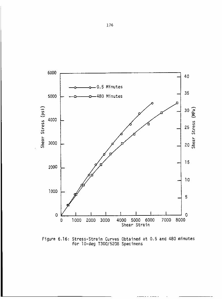
176
6OOO
50OO
A
V
4000
C_
3000
2000
lO00
0.5 Minutes
- _480 Minutes
o I l I0 I000 2000 3000
I I I
4000 5000 6000
Shear Strain
- 40
-- 35
-- 5
I o7000 8000
30 _=
25 •
t._
20 -_
15
lO
Figure 6.16: Stress-Strain Curves Obtained at 0.5 and 480 minutes
for lO-deg T300/5208 Specimens
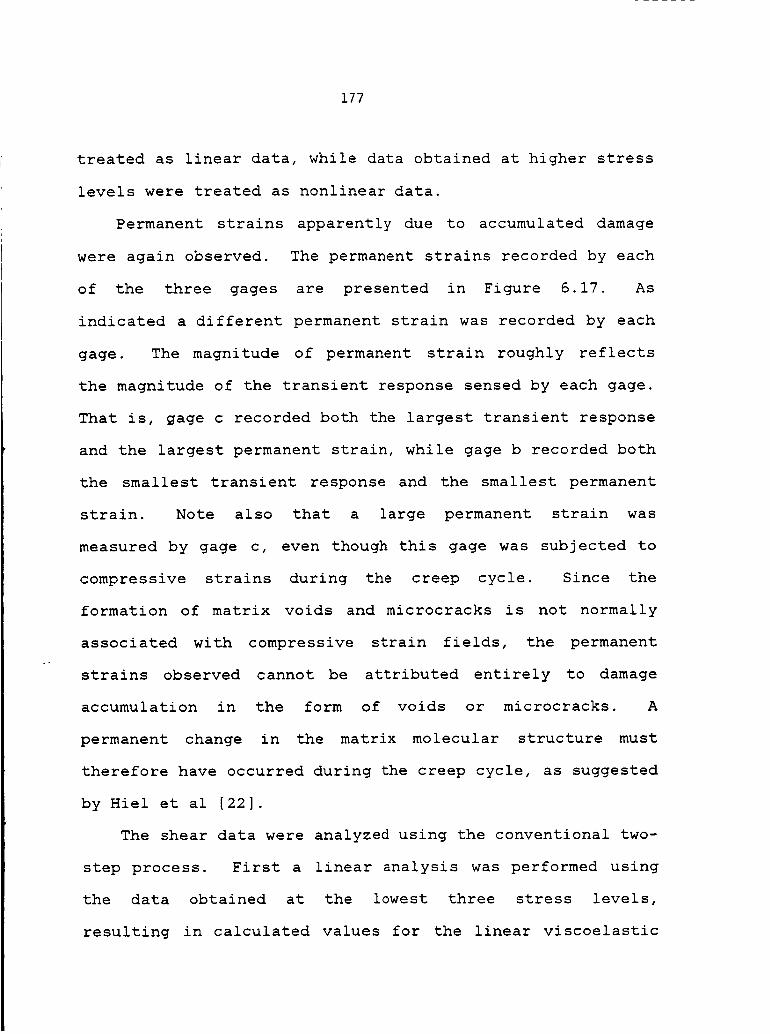
177
treated as linear data, while data obtained at higher stress
levels were treated as nonlinear data.
Permanent strains apparently due to accumulated damage
were again observed. The permanent strains recorded by each
of the three gages are presented in Figure 6.17. As
indicated a different permanent strain was recorded by each
gage. The magnitude of permanent strain roughly reflects
the magnitude of the transient response sensed by each gage.
That is, gage c recorded both the largest transient response
and the largest permanent strain, while gage b recorded both
the smallest transient response and the smallest permanent
strain. Note also that a large permanent strain was
measured by gage c, even though this gage was subjected to
compressive strains during the creep cycle. Since the
formation of matrix voids and microcracks is not normally
associated with compressive strain fields, the permanent
strains observed cannot be attributed entirely to damage
accumulation in the form of voids or microcracks. A
permanent change in the matrix molecular structure must
therefore have occurred during the creep cycle, as suggested
by Hiel et al [22].
The shear data were analyzed using the conventional two-
step process. First a linear analysis was performed using
the data obtained at the lowest three stress levels,
resulting in calculated values for the linear viscoelastic
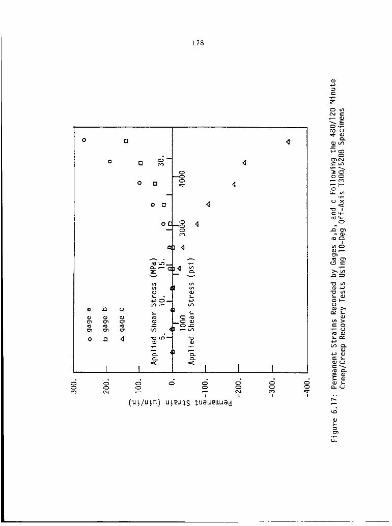
178
0
¢0
o
0
I
Q
4
o
o
,4
I
,S0q,.j!
I,::5
I
4
_S
!
*=se-°_
C',,Ie-'
_E
CO
_¢./3e-+_CO
e-l._
0_
O0
0
_'.4--_tl--
!
mC:_I:D r---
_'_
Ol'--
e- 0
c_ _.
E _
°°
._,=.I.u.
179
parameters Ao, C, and n. The remaining nonlinear parameters
were then calculated using the nonlinear data obtained at
the higher stress levels.
Linear Analysis
A linear analysis was performed using the creep data
obtained at shear stress levels of 2.9, 6.1, and 8.8 MPa.
Unsatisfactory results were obtained for the lowest stress
level of 2.9 MPa. The C and n values calculated using this
data set were 0.01297 X I/GPa-min n and 0.083, respectively,
which do not compare well with the results listed below,
which were obtained at the other two stress levels. This
discrepancy was probably due to the very low viscoelastic
response, since the total transient shear strain measured
over the 480 minute creep period was only 30 _in/in.
Therefore, it was assumed that accurate measurement of C and
n could not be obtained using this data set, and the above
values were not used in the analysis.
The average values for A o, C, and n calculated using the
creep data obtained at 6.1 and 8.8 MPa were
A ° = 0.1561 _ 0.001115 ( X I/GPa)
= 1.0761 + 0.00769 ( X 10-6/psi)
C = 0.00332 + 0.000140 ( X I/GPa-min n)
= 0.0229 t 0.000962 ( X 10-6/psi-min n)
n = 0.247 + 0.0214
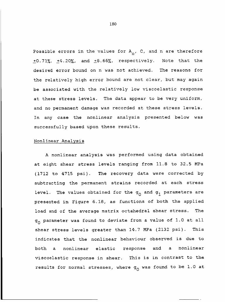
180
Possible errors in the values for Ao, C, and n are therefore
Z0.71%, _4.20_, and ±8.66_, respectively. Note that the
desired error bound on n was not achieved. The reasons for
the relatively high error bound are not clear, but may again
be associated with the relatively low viscoelastic response
at these stress levels. The data appear to be very uniform,
and no permanent damage was recorded at these stress levels.
In any case the nonlinear analysis presented below was
successfully based upon these results.
Nonlinear Analysis
A nonlinear analysis was performed using data obtained
at eight shear stress levels ranging from 11.8 to 32.5 MPa
(1712 to 4715 psi). The recovery data were corrected by
subtracting the permanent strains recorded at each stress
level. The values obtained for the go and gl parameters are
presented in Figure 6.18, as functions of both the applied
load and of the average matrix octahedral shear stress. The
go parameter was found to deviate from a value of 1.0 at all
shear stress levels greater than 14.7 MPa (2132 psi). This
indicates that the nonlinear behaviour observed is due to
both a nonlinear elastic response and a nonlinear
viscoelastic response in shear. This is in contrast to the
results for normal stresses, where go was found to be 1.0 at
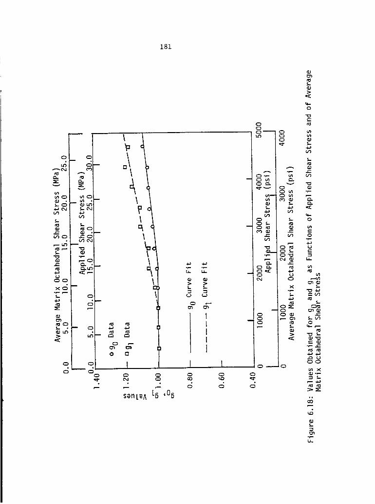
181
o-ol
0o
L-_ 01-
r--O
_JO0
xO
t_ . -- _
0
'l°\
I:l
I_ 0
san LEA 1-6 ,06
> >_= _=
IIIII
I I0 _
v_
x
"[
p. t_
>
o
MI
%=
or}
0_
0
00_
u_=..=_I=_
_=
0
_n x
•-_ L
_d

182
all normal stress levels, i.e., the elastic response was
linear at all normal stress levels. A bilinear fit of the
go data for use with the VISLAP program resulted in
< 12.05 MPa
1.0 , for Toc t _
g0 (Toct)=
1.0 + 5.48 x 10 -3 (Toc t - 12.05), for Toc t > 12.05 MPa
The gl parameter was also found to be stress dependent.
A bilinear fit of the gl data resulted in
< 7 23 MPa
"i.0 , for Toc t _ .
gl (Toct) =
1.0 + 9.79 x 10⁻³ (_oct - 7.23), for Toct > 7.23 MPa
The bilinear curve fits of the go and gl parameters are
shown in Figure 6.18 as solid and dashed lines,
respectively.
The results obtained for the g2 parameter are presented
in Figure 6.19. This parameter was found to be most
sensitive to shear stress, ranging from a value of 1.0 at
linear stress levels to about 3.6 at a shear stress of 32.5
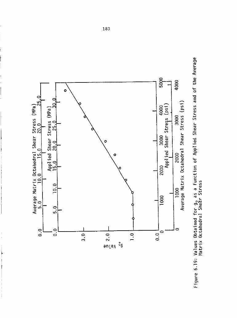
183
v
=_
m
_ ¢_
°f--
-&=C_.LO --•=C r--
0
m
LO
_O_m o
°t__° I I
en LEA Z6
A I
0.,-- I
co.._c_
Q;P
_
v
c'_ L
Q;
C',4_
X
4._
et_
t
<
O
t
O
o*p
_J
0
•_- .._
x_._"_--
_m
g
_J
u..
184
MPa (4715 psi). The g2 data were also fit using a bilinear
function, resulting in
g2octIi° for°ct723 a.0 + 0.124 (Toc t - 7.23), for • > 7.23 MPa
oct
This function is shown as a solid line in Figure 6.19.
The results obtained for a ° are presented in Figure
6.20.The data for a ° exhibited considerable scatter, and
no truly distinctive pattern emerged. As previously noted
the a° function was expected to exhibit an exponential
dependence with stress. Therefore, the data were
characterized using the following exponential function
I < 14.5 MPa
1.0, for Toc t _
so(Toe t) =
-0.0340 (Toct - 14.5),e for roct > 14.5 MPa
The above relation is shown as a solid line in Figure 6.20.

185
v
4-_0
c-O0
c-
U
X
_:Sr--
m •
0 m¢0
v
(./I
s..
or-
Q. LO
• I
m
0l •
0
o
o
I I I
D
anLE A E
0O
Lg') ,.-,-I oQ
_._ ,_ __
i
it'M !
o')r_
(1.1
c.-
4-0
"0<-.
0')
.T,--I-.)
c-.-
c-r._ "1:3
u
I,. u4-_ e-
_ mt_ ¢o
I.
e- c-
¢o4-_ r,.-
U'_ q,l
d:;_M
t_
°,p.

VII. LONG TERM EXPERIMENTS
One of the major objectives of this study was to obtain
experimental measurements of the long-term creep compliance
of composite laminates. In previous studies at VPI&SU,
compliance measurements were obtained for a maximum time of
104 minutes (6.9 days). It was felt that measurements at
longer times were required so as to provide a more rigorous
check of the long-term predictions obtained via the
accelerated characterization scheme described in previous
chapters. The efforts to obtain these long-term
measurements will be described in this chapter.
Selection of the Laminate Layups
Two distinct laminate layups were to be tested during
the long-term tests. The laminates were selected such that
the stress state applied to the individual plies would
differ significantly, so as to produce two distinct
viscoelastic responses. A constraint on laminate selection
was imposed by the material shortages previously mentioned.
Due to these shortages, all long-term specimens had to be
fabricated from a single [0/30/-60/0] s panel of T300/5208
graphite-epoxy. This panel was fabricated in the VPI&SU hot
press facility, using the same NARMCO RIGIDITE 5208 prepreg
tape and heat/pressure cycle used to fabricate the
186

187
unidirectional specimens. Different laminate layups could
only be obtained by sawing specimens from the parent panel
at various angles away from the 0-deg fiber directions.
Thus, potential laminate layups for the tensile specimens
were defined by an angle $ ranging from 0 to 180 degrees, as
depicted in Figure 7.1.
To aid in laminate selection, an analysis of the
potential layups was performed using conventional (elastic)
CLT. The results of this analysis are presented in Figure
7.2, where the transverse normal stress and shear stress
induced in each ply as a function of the angle B are
plotted. The laminate layups selected for testing are
denoted by the dashed lines in Figure 7.2. The first was a
[I00/-50/_0/I00] s laminate, or equivalently, a
[-80/-50/_0/-80] s laminate. This laminate was selected
because all plies were subjected to relatively high
transverse normal and shear stresses, as indicated in Figure
7.2. The [-80/-50/40/-80] s laminate will be referred to as
laminate "A". The second layup chosen was a [20/50/-40/20] s
laminate. This layup results in relatively high shear
stresses in all plies but relatively low transverse normal
stresses. The [20/50/-%0/20] s laminate will be referred to
as laminate "B"
Static tensile tests to failure at a temperature of 149C
(300F) were conducted for both laminates. Ultimate
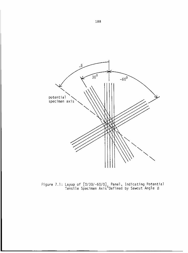
188
\\
potential ._specimen axls
\
_60 o
\\
\\
Figure 7.1- Layup of [0/30/-60/0] Panel, Indicating PotentialTensile Specimen AxisSDefined by Sawcut Angle B

189
x
_00"2520
_ 0.15
t_f..
_ E_ _- O.lOe- o_zL
_- 0.05
N,_
-- 0.00
E
o -0.05Z
0°oP]Ys
.lu Klys-_ -60"Plys
AI
- iB
_ I
0.20
0°_Plys
__ 30_0 Plys-60 Plys
II10 40 80 1(DO 120 140
i B (degrees)
II1I
Figure 7.2: Transverse Normal and Shear Stresses Induced in Each
Ply by an Applied Normal Stress _x as a Function ofSawcut Angle
190
strengths of 136 and 271 MPa (19660 and 39320 psi) were
measured for laminates A and B, respectively. Thus, the
ultimate strength of laminate B was approximately twice as
high as that of laminate A. The long-term creep tests were
conducted at stress levels of 76 and 156 MPa (II000 and
23000 psi) for laminates A and B, respectively. These
stress levels correspond to roughly 60_ of the laminate
static ultimate strengths.
As mentioned in Chapter VI, a five-station creep frame
was used during the long-term study. Hence it was possible
to test five specimens concurrently. Three specimens of
laminate A and two specimens of laminate B were tested.
Drift Measurements
The long-term specimens were strain gaged with gages
mounted back-to-back, as described for the unidirectional
specimens in Chapter VI. Strains were measured using a
Vishay P-350 portable digital strain indicator and a SB-IK
ten channel switch and balance unit. An initial concern was
that electronic "drift" of the gage signal might occur over
the 105 minute test period. Drift can result from a variety
of factors, including a change in strain gage or leadwire
resistance, a change in strain gage gage factor, or
amplifier instabilities. Since the laminate creep rate was
expected to be rather low at long times, it Has possible
that drift could mask the actual viscoelastic response at
191
long times. The effective drift rate was therefore
monitored during testing by placing separate Wheatstone
bridge "drift" circuits within three test ovens, immediately
adjacent to the mechanically-loaded tensile specimens. The
drift specimens were gaged and wired exactly as the tensile
specimens. At the start of the creep test, the drift
circuits were balanced to zero, and the output of each
circuit was monitored throughout the test.
Two of the three circuits indicated very low drift.
After 105 minutes one had measured a total drift of 17
_in/in, while the second had measured 35 _in/in, indicating
an average drift rate of 0.37 _in/in/day. The third drift
circuit initially indicated a very low drift rate as well.
However, after about 20000 minutes (5.5 days) substantially
higher (and unreasonable) drift rates were observed. This
third circuit finally failed after 57900 minutes (40 days).
The final reading taken from this circuit was 734 _in/in,
which was of the same magnitude as the total transient
response measured until that time for the loaded specimens.
Thus, it is concluded that the high drift rate indicated by
this circuit was due to a faulty strain gage or solder
joint, and the data obtained from this circuit were
discarded.
The two drift circuits which did survive the total test
period indicated that drift might account for perhaps 20-50
192
_in/in of the transient response recorded over the 105
minute period. On the other hand, the transient reponse was
on the order of I000 _in/in. The effects of drift were
therefore estimated to be less than 5_ of the transient
response, and were neglected during the data reduction and
analysis.
Specimen Performance
As described above, three specimens of layup A and two
specimens of layup B were tested. After initiation of the
long-term tests, two of the specimens of layup A apparently
failed, the first after 14960 minutes (10.4 days) and the
second after 46915 minutes (32.6 days). Since the ovens are
not equipped with windows, it was not possible to view the
specimens from outside of the test ovens. It was also
undesirable to open the ovens for inspection since the other
tests would likely be disturbed. Therefore, the "failed"
specimens were left undisturbed for the entire 105 minute
testing period. However, upon completion of the test it was
discovered that these specimens had not failed but rather
had merely slipped out of the upper specimen grips. In
retrospect, it would have been advisable to use pins through
the grips and specimens to prevent such slippage. Pins were
used to prevent slippage of the B specimens, since these
were tested at a much higher stress level. Short-term tests
had been conducted at the specimen A stress level (76 MPa)

193
and no slipping had been observed. Therefore, slippage was
not expected.
The third A specimen remained loaded for the entire 105
minute test period, but the strain gage circuit for this
specimen failed after 34895 minutes (24.2 days). Reasonable
strain measurements were obtained for this specimen until
shortly before gage failure. Inspection following test
completion revealed that the solder joint bonding the
preattached leadwire ribbon to the gage tab had failed.
Due to these mechanical and electrical difficulties,
results for the A laminate were obtained for a maximum time
of 46915 minutes. While this was far short of the intended
105 minute test period, it was still a major increase in
previous long-term test times.
Data for the two B laminates were obtained for the
entire test period. Deformation of the B specimens occurred
in a smooth and uniform manner, with no indication of any
gage failures or excessive gage drift. The measured results
for both the A and B laminates will be compared to the long-
term response predicted by the program VISLAP in the
following chapter.

VIII. COMPARISON BETWEEN PREDICTION AND MEASUREMENT
In previous chapters, the accelerated viscoelastic
characterization of unidirectional specimens of T300/5208
graphite-epoxy was described. During characterization, a
series of creep/recovery tests were performed at several
stress levels and at a temperature of 149C (300F), using
both 90-deg and 10-deg off-axis specimens. These short-term
results may be used in conjunction with the lamination
program VISLAP to provide predictions of the long-term
viscoelastic response of T300/5208 composite laminates of
arbitrary layup. To check the accuracy of these
predictions, long-term creep tests were conducted using
specimens with two distinct layups. Laminate A, consisting
of a [-80/-50/40/-80] s layup, was selected because for this
layup all plies are subjected to relatively high transverse
normal and shear stresses. Laminate B, consisting of a
[20/50/-40/20] s layup, was selected because for this layup
all plies are subjected to relatively high shear stresses
but relatively low transverse normal stresses. The ultimate
strength of laminate B was slightly greater than twice that
of laminate A. Both laminates A and B were tested at creep
stress levels of approximately 60_ of ultimate; laminate A
was tested at 76 MPa (II,000 psi), while laminate B was
tested at 156 MPa (23,000 psi). The viscoelastic response
194
195
of laminate A was expected to be significantly greater than
that of laminate B.
The predicted and measured compliances for laminates A
and B are presented in Figures 8.1 through 8.4. The
comparison for laminate A is made in Figures 8.1 and 8.2,
where the vertical compliance scale in Figure 8.2 is
expanded relative to Figure 8.1, to provide a clear
comparison between theory and experiment. The corresponding
comparison for laminate B is presented in Figures 8.3 and
8.4. The comparison is similar for both laminates, in that
a reasonably accurate prediction of the instantaneous
(elastic) response was obtained, but at increased times the
predicted response falls below the measured response. For
laminate A the average measured compliance at 14960 minutes
(the longest time at which all three A laminates were still
functional) was approximately i0_ higher than predicted.
Figure 8.1 indicates that at longer times the differences
between the average and predicted response would have been
greater still. For laminate B, the average measured
compliance at 105 minutes was approximately 12_ higher than
predicted.
Recall that a 480 minute creep time was used during the
accelerated characterization tests using unidirectional
specimens. The Schapery theory was applied to these data,
and in each case the predicted and measured response
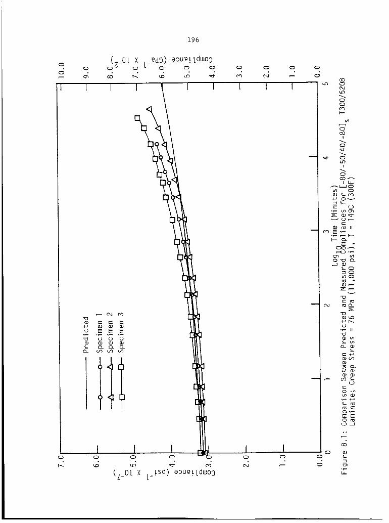
00
0
196
I I
(_ OL X L_0dg) aoU_.LLdwo_)0 0 0 _ 0
I 1 I I
_ E E E• _-- ._,- °7-,- °r--
_ c7 _ e7
<
IO
IO
(z_OL x
0 Cb 0 0
I I I
I I0 0
:.j ,-
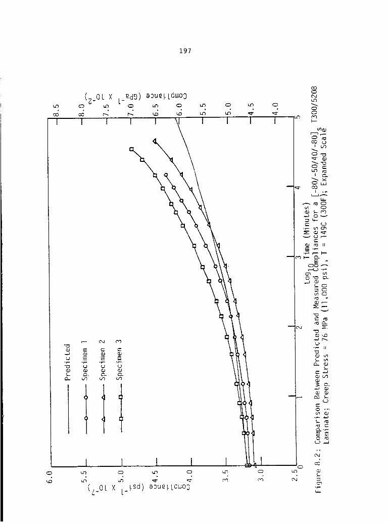
197
CD
LO
I
(z_OL xCD
i _dD) a_ue_Ldwoo
I I I
,,--.- ¢_1 ¢0
°e.- •e.,-, .I.- ,e..-
(,.,0 oO oO
I 1 I I
(/.OL X _sd) _U_L LdtUO0k-"
I 1 I
O00
CD
I--
CO
I __.X
LI-
u_ CD
•_-- _,o 0'_
_ II
_.,.-
_ ,...-
°_'- H
N O-
0 • '"m _
¢._ e'-
_ -.J
.°
d
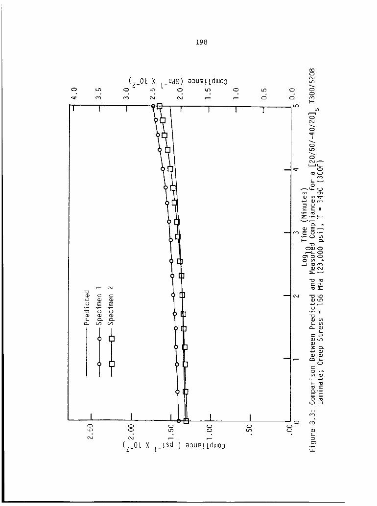
198
0
(__OL0
_4
X L_edg) a_Ue_Ldw0D0
I
c;
I
I I0 0
(z_OL
0L._
r'.--
LsdL-
I I00
aaue L.Ldw0o
0I..0

199
C-J
(_ OL XG- _ L-
_4
I
_ t-- e-
°_-- .r,-- .f--
I I I I
(L_OL X L_.Lsd) _u_.Lld_0D
1 I
v
°1--
_,_ r,,',.,.
0
CO ¢1
0 X
0
0
c- _ II°_,-
U
"_- II
m
mm __0
@
°e-
200
compared favorably. Typical results have been presented in
Figures 6.3-6.5. It had therefore been anticipated that a
good comparison for the laminates would be achieved over at
least this shorter time period. Inspection of Figs. 8.2 and
8.4 indicates discrepancies between the slopes of the
measured and predicted compliance curves even at short
times, however. Although the magnitudes of the predicted
and measured responses at short times are reasonably close,
this simply reflects the accuracy of conventional (elastic)
CLT. Thus, the error observed is mainly due to an
inaccurate modeling of the laminate viscoelastic response.
The long-term laminate tests were conducted using a five
station creep frame which had been fabricated in-house. The
short-term tests on the other hand were conducted using a
commercially available single station ATS creep frame. The
test ovens used with the five station frame were known to
produce relatively high thermal gradients, as compared to
the ATS test oven. Therefore, it was suspected initially
that the long-term specimens had been subjected to test
temperatures higher than the intended test temperature of
149C, which could account for the discrepancies observed
between predicted and measured response. However this is
considered unlikely for two reasons. First, the oven
control thermocouple was mounted to within about 0.64 cm
(0.125 inch) of the strain gage site on each of the

201
mechanically loaded specimens. Even if significant thermal
gradients existed along the length of the specimens, the
material in the vicinity of the strain gage site was
maintained at a temperature very near 149C. Also, nominal
specimen thicknesses were 0.I0 cm (0.04 inch), and so
significant through-thickness thermal gradients were
unlikely. Secondly, there was little discrepancy between
predicted and measured results in initial elastic response.
If the long-term test temperature had been appreciably
higher than desired, a poor comparison between predicted and
measured elastic response would have been observed.
Note that the measured viscoelastic response recorded
for both laminates is very consistent and uniform from
specimen to specimen. The experimental curves could be
shifted up or down to form a distinct response curve for
each laminate type. Discrepancies are due for the most part
to small differences in the inital elastic response. This
repeatable viscoelastic response from specimen to specimen
as well as the very low strain gage drift rates previously
noted tends to increase confidence in the measured results.
Based upon these observations, it must be concluded that
some mechanism impacting the viscoelastic response of
composite laminates has not been properly accounted for in
the VISLAP analysis. It is possible that the viscoelastic
parameters determined during the short-term tests were

202
calculated in error, causing discrepancies at long times.
This would not explain the errors at short times, however.
One portion of the present analysis which may be suspect
is the manner in which the effects of biaxial stress fields
have been accounted for. Recall that the average matrix
octahedral shear stress has been used to account for such
stress interactions, using a mechanics of materials approach
to determine the average matrix stresses. Perhaps this
approach is too simple to characterize the effects of the
complex three-dimensional stress state which exists at the
micromechanics level at all fiber/matrix interfaces. The
problem may be further accentuated at interfaces between
alternating plies within the composite laminate.
Another area of concern is the accumulation of damage
during the creep process, which has been observed during
both the present study and in previous efforts [22].
Evidence suggests that this permanent damage is due to both
the formation of voids and microcracks within the composite
matrix material and permanent changes in the matrix
molecular structure. It has not been possible to correct
the unidirectional creep data for damage accumulation,
although an attempt was made to correct the unidirectional
recovery data by subtracting out any permanent strains
recorded. A portion of the creep response is therefore due
to viscoelastic mechanisms, while a portion is presumably

203
due to fracture mechanisms. This implies that the
viscoelastic parameters calculated using the creep data may
reflect to some extent the initial damage state of the
specimen as well as the amount of damage accumulated during
testing. This problem could be alleviated somewhat if the
unidirectional specimens were mechanically conditioned prior
to testing, but as previously noted this would not
correspond to a practical situation. Furthermore, the
damage which occurs in a unidirectional composite specimen
is not necessarily representative of the damage which occurs
in a composite laminate. Laminate damage may occur in
various combinations of matrix cracking, fiber-matrix
_-_-- =-- delamination ....... p ,_=__, u_cw_ _±_ or local fiber
breakage. Many of these failure modes do not occur in
unidirectional specimens. The type and extent of damage
which occurs in a laminate depends upon stacking sequence,
fabrication techniques, geometry, applied loads, and loading
history [61,62]. Due to these effects, it may not be
possible to characterize damage accumulation within a
laminate based solely upon results obtained from
unidirectional specimens.
Finally, note that the VISLAP analysis is based upon
CLT, with slight modification to account for viscoelastic
behaviour. If the analysis is to be valid, the principal
assumptions associated with CLT must be satisfied. Namely,

204
the plane stress assumption and the Kirchoff hypothesis.
Thus, interlaminar shear deformations are not considered in
the VISLAP analysis. As a result, laminates with three or
more fiber directions possess a theoretical upper bound on
compliance, as pointed out by Dillard et al [22]. In
practice, however, laminates may undergo significant
viscoelastic interlaminar shear deformations and
subsequently may have no upper bound on compliance. This
shortcoming could be resolved if some method to integrate
interlaminar shear deformations within lamination theory
could be formulated. The only alternative would be to
discard the present approach and utilize a more
sophisticated (and more expensive) method such as the finite
element technique.

IX. SUMMARY AND RECOMMENDATIONS
Summary of Results
In this study an accelerated characterization technique
was applied to T300/5208 graphite-epoxy composites. The
study utilized a characterization procedure previously
developed at VPI&SU. The basic concept is to use short-term
test data, obtained from unidirectional specimens, to
predict the long-term behaviour of composite laminates of
arbitrary layup. Previous efforts had focused exclusively
on the T300/934 graphite-epoxy material system. Therefore,
the T300/5208 material system was selected for use in the
present study, to determine if the accelerated
characterization scheme could be confidently applied to
materials other than T300/934. Improvements in the
characterization scheme were also implemented during this
study, in the form of a more accurate viscoelastic
compliance model and in improved short-term testing
procedures.
Each of the six program objectives listed in Chapter I
were achieved during the course of the study. First, the
Schapery nonlinear viscoelastic theory was integrated with
the accelerated characterization scheme. A recursive
relationship was developed, based upon the Schapery theory.
2O5
206
This expression gives the nonlinear viscoelastic response at
time tj, following j-steps in stress. This allows
calculation of the nonlinear viscoelastic response to a
complex uniaxial load history. The complex load may be
approximated to any degree of accuracy by using discrete
steps in stress. The recursive relationship was integrated
with an existing lamination computer program called VISLAP,
allowing predictions of the long-term viscoelastic response
of composite laminates.
The impact on long-term predictions induced by an error
in one of the seven Schapery viscoelastic parameters was
also investigated. The approach used was to calculate the
predicted response using an "incorrect" value for the
parameter of interest but the "correct" value for all other
parameters. The prediction calculated using the erroneous
parameter was then compared with the exact response. It was
concluded that in the present case long-term predictions
were most sensitive to error in the power law exponent n.
It was noted however that this conclusion is contingent upon
the length of prediction desired as well as the viscoelastic
properties of the specific material being investigated. The
above conclusion was based upon typical properties of
T300/5208 and a maximum prediction time of 105 minutes. It
is recommended that a similar analysis be performed if a
different material is studied or if different prediction
207
times are required. However, as a general rule, long-term
predictions are most sensitive to errors in n.
The data reduction techniques used to calculate the
linear viscoelastic parameters Ao, C and n were also
investigated. It was shown that in theory these parameters
can be calculated using either linear creep or linear
recovery data, i.e., the use of either creep or recovery
data is theoretically equivalent. Consideration was then
given to the type of experimental strain measurement errors
likely to occur in practice. It was found that the power
law exponent was sensitive to even small offset errors in
recovery data, but insensitive to offset errors in creep
data. Small offset errors in the recovery data were
considered likely due to damage accumulation and slight
strain gage zero drift _,,_ +_...... _ _,,e creep cycle. Therefore,
it was concluded that the linear viscoelastic parameters
should be calculated using creep data.
A short-term creep/recovery testing cycle was selected
which was keyed towards an accurate measure of the power law
parameter n. The testing cycle was based upon strain gage
accuracy and sensitivity, the expected viscoelastic response
for T300/5208 at 149C, and a specified prediction accuracy
of _I0_ at the maximum prediction time of 105 minutes.
These considerations led to the selection of a 480/120
minute creep/recovery testing cycle. The concepts used in

2O8
selecting this cycle were also collected and listed as a
proposed standard test selection procedure. This standard
process should provide useful guidelines to the researcher
studying a viscoelastic material which has not been
previously investigated.
The 480/120 minute creep/recovery cycle was used to
characterize the viscoelastic response of unidirectional
specimens of T300/5208 graphite-epoxy. The viscoelastic
response to transverse normal stress was characterized using
90-deg off-axis tensile specimens, while the response to
shear stress was characterized using 10-deg off-axis tensile
specimens. For the transverse case, nonlinear behaviour was
observed at stress levels greater than about 15.6 MPa (2250
psi). However, it was also noted that nonlinear behaviour
may occur at lower stress levels but may not become apparent
for very long times. For the case of shear stress nonlinear
behaviour was observed at stress levels greater than about
8.8 MPa (1279 psi). Nonlinear effects were much more
significant in the case of shear stress than in the case of
transverse normal stress.
Predictions obtained using the program VISLAP were
compared to measured results for two distinct laminate
layups. Comparisons were made for a maximum time of 105
minutes. It was found that although the predicted
instantaneous response compared well with measured results,
209
the predicted viscoelastic response was significantly less
than the measured viscoelastic response. Thus, the
predicted response was non-conservative. The discrepancy
between theory and experiment is believed to be due to an
insufficient modeling of stress interaction effects within
individual plies, to damage accumulation within individual
plies, and/or to interlaminar shear deformations which
develop during the viscoelastic creep process.
Although the comparison between theory and experiment
obtained during this study is far from exact, it is believed
that the fundamental approach used is valid. The
accelerated characterization of composite laminates is a
difficult problem, involving elements of lamination theory,
nonlinear viscoelasticity, and fracture mechanics, among
others. Accelerated characterization is an important
research topic, however, due to the potential long-term
viscoelastic response of composite laminates. A variety of
load-bearing structural components fabricated from
composites are being introduced into the marketplace. It is
therefore important that the long-term viscoelastic response
of composites be well understood and anticipated at the
design stage.
Recommendations
A major question during application of the Schapery
210
theory in the present study was how to account for permanent
damage. Damage has been attributed at least in part to the
formation of voids and microcracks in the composite matrix
material during creep. These voids and microcracks are in
turn due in part to the highly heterogeneous nature of
composites at the micromechanics level. Complex three
dimensional stress states exist near fiber-matrix interfaces
and near free edges, resulting in matrix cracks at applied
stress levels far below the effective ultimate strength of
the composite. It is believed that problems with damage
accumulation could be minimized by using a "simpler"
material, i.e., a homogeneous, initially isotropic,
nonlinear viscoelastic material. Also note that in the
present study the validity of the long-term predictions of
the Schapery theory has been obscured since the Schapery
results were not used directly but rather were combined
using lamination theory to predict the long-term response of
a laminate. Therefore, it is suggested that portions of
this study be repeated with a "simple" material.
Specifically, it is suggested that the Schapery analysis be
applied as described herein to a homogeneous viscoelastic
material, e.g., polycarbonate, and compared with long-term
measurements. Such a study would indicate the level of
accuracy possible using accelerated characterization
techniques, and if successful would confirm that the

211
difficulties in long-term prediction encountered herein were
due to the laminate analysis and not due to the short-term
characterization process. Alternatively, the Schapery
theory could be validated by predicting the response to a
time-dependent loading history such as a ramp loading
function or a low-frequency sinusoidal loading function.
Response to such a load history could be approximated using
the recursive relationship presented herein (eq. 3.10), or
by integrating the Schapery single-integral expression (eq.
3.1) directly. If this latter approach were used a closed-
form solution to eq. 3.1 may not be obtainable, requiring
numerical integration. Peretz and Weitsman have used this
approach in their studies on FM-73 [50].
In the present study the average matrix octahedral shear
stress, _oct' has been used to account for the effects of
biaxial stress states on the viscoelastic response, where
_oct was calculated using a mechanics of materials model.
Although this approach has been used in previous studies
[21,35], to the author's knowledge the validity of this
model has not been confirmed. It is suggested that creep
tests be conducted using a biaxial loading state, e.g.,
static loads applied both parallel and perpendicular to the
fiber direction. Although biaxial loading would be more
difficult to apply than uniaxial loads, the test results
would directly prove or disprove the average matrix
212
octahedral shear stress model. An alternate approach would
be to use uniaxial test results for several different off-
axis tensile specimens. In this case, the ratio of the
loads applied parallel and perpendicular to the fibers is
fixed by the specimen fiber angle. Although these tests
would be much easier to perform than an externally applied
biaxial load test, the selection of load ratios would be
somewhat restricted.
A final recommendation involves possible interlaminar
shear deformations which may occur during the viscoelastic
creep process. A finite element analysis should be
conducted for a few laminates to determine the contribution
to creep due to interlaminar shear strains. If interlaminar
effects are appreciable these must be incorporated into the
CLT analysis. Otherwise, the relatively simple and
inexpensive analysis possible using VISLAP must be replaced
with a more complex and expensive procedure, probably based
upon a finite element analysis of each laminate considered.
References
(I) Pikes, R.B., and Pagano, N.J.,"Interlaminar Stresses in
Composite Laminates Under Uniform Axial Extension",
J. Composite Materials , Vol. 4, 1970, pg 538.
(2) Wang, A.S.D., and Crossman, F.W.,"Some New Results on
Edge Effect in Symmetric Composite Laminates",
J. Composite Materials , Vol, II, 1977, pg 92.
(3) Herakovich, C.T.,"On the Relationship Between
Engineering Properties and Delamination of Composite
Materials", J. Composite Materials , Vol. 15, 1981, pg 336.
(4) Quinn, W.J., and Matthews, F.L.,"The Effect of Stacking
Sequence on the Pin-Bearing Strength in Glass-Fibre
Reinforced Plastic", J. Composite Materials , Vol. ii, 1977,
pg 139.
(5) Ford, J.L., Patel, H.P., and Turner, J.L. "Interlaminar
Shear Effects in Cord-Rubber Composites",
Fibre Science and Technology , Vol 17, 1982, pg 255.
(6) Simitses, G.J., and Giri, J.,"Buckling of Rotationally
Restrained Orthotropic Plates Under Uniaxial Compression",
J. Composite Materials , Vol II, 1977, pg 249.
(7) Hewson, p. , '_,c_]i_g.............._f Pl]]truded Glass Fibre-Reinforced
Channel Sections", Composites , Vol 9, 1978, pg 56.
(8) Hyer, M.W.,"Nonlinear Effects of Elastic Coupling in
Unsymmetric Laminates",Presented at the IUTAM Symposium on
Mechanics of Composite Materials, 1982, VPI&SU, Blacksburg,
Virginia.
(9) Crawley, E.F.,"The Natural Modes of Graphite-Epoxy
Cantilever Plates and Shells", J. Composite Materials , Vol
13, 1979, pg 195.
(I0) Chao, C.C., and Lee, J.C.,"Vibration of Eccentrically
Stiffened Laminates", J. Composite Materials , Vol 14, 1980,
pg 233.
(II) Kibler, K.G.,"Effects of Temperature and Moisture on
the Creep Compliance of Graphite-Epoxy Composites", AGARD
Conf Proc No. 288,
Effect of Service Environment on Composite Materials
AGARD-CP-288, 7 Rue Anuelle, 92200 Neuilly, Sur Seine,France.
213

214
(12) Shen, C.H., and springer, G.S. "Effects of Moisture andTemperature on the Tensile Strength'of Composite Materials",j. Composite Materials , Vol II, 1977, pg 2.
(13) Loos, A.C., and springer, G.S.,"Effects of Thermal
Spiking on Graphite-Epoxy Composites",
j. Composite Materials , Vol 13, 1979, Pg 17.
(14) Adamson, M.J.,"A Conceptual Model of the Thermal Spike
Mechanism in Graphite-Epoxy Laminates", Presented at the
ASTM Conference on Long-Term Behaviour of Composite
Laminates, Williamsburg, Virginia, March 1981 (to appear in
the Conference Proceedings)-
(15) Rotem, A., and Nelson, H.G. "Fatigue Behaviour of
Graphite-Epoxy Laminates at Elevated' Temperatures", NASA TM
81150, 1979.
lliams, D.p.,"Effects of
) Sumison, • ",E_ironment H T and Wion the Fatigue of Graphite-Epoxy Composites"
ASTM STP 569, 1975.
(17) Sumison, H.T. ,,Environmental Effects on Graphite-EpoxyFatigue Prop erties'_ j Spacecraft and Rockets , Vol 13, No
3, 1976.
(18) Yeow, Y.T., Morris, D.H., and Brinson, H.F.,"The Time-
Temperature Behaviour of a Unidirectional Graphite-EpoXy
Composite", ASTM STP 674, 1979 (see also VPI&SU Report, VPI-
E-78-_, February, 1978).
19) Griffith, W.I., Morris, D.H., and Brinson, H.F.,"The
_ccelerated Characterization of Viscoelastic Composite5 April 1980.' _ S"Materla_ , VPI&SU Report, VPI-E-80-1 ,
(20) Griffith, W.I., Morris, D.H., and Brinson,
H.F. "Accelerated Characterization of Graphite-Epoxy
Composites", VPI&SU Report VPI-E-80-27, September 1980.
(21) Dillard, D.A., Morris, D.H., and Brinson, H.F., "Creep
and Creep Rupture of Laminated Graphite-Epoxy Composites",
VPI&SU Report, VPI-E-81-3, March 1981.H.F.,"The
(22) Hiel, C., Cardon, A.H., and Brinson,Nonlinear Viscoelastic Response of Resin Matrix Composite
Laminates", VPI&SU Report, VPI-E-83-6, March 1983.
) Brinson, H.F., Morris, D.H., and Yeow, y.T.,"A New
E_erimental Method for the Accelerated Characterization of

215
Composite Materials"• Proc 6th Int Conf on Experimental
Stress Analysis• Munich• 1978, pg 395.
(24) Jones• Robert M., Mechanics of Composite Materials ,McGraw-Hill, New York, 1975.
(25) Morris• D.H., Brinson, H.F.• and Yeow• Y.T.,"The
Viscoelastic Behaviour of the Principal Compliance Matrix of
a Unidirectional Graphite-Epoxy Composite"•
Polymer Composites , Vol I• No. I, 1980, pg 32.
(26) Moehlenpah• A.E.• Isha, 0.• DiBenedetto• A.T.• "The
Effect of Time and Temperature on the Mechanical Behaviour
of Epoxy Composites"• Polymer Engineering and Science • Vol
II, No 2• March 1971• pg 129.
(27) Miyano, Y., and Kansmitsu, M.,"Time and Temperature
Dependence of Flexural Strength in Transversal Direction of
Fibres in CFRP" Fibre Science and Technology , Vol 18
1983, pg 65.
(28) Ferry, J.D., Viscoelastic Properties of Polymers , John
Wiley and Sons, New York, 1970.
(29) Hahn, H.T.,"Nonlinear Behaviour of Laminated
Composites", j. Composite Materials , Voi 7, 1973, pq 257.
(30) Findley, W.N., and Peterson, D.B.•"Prediction of Long-
Time Creep With Ten-Year Creep Data on Four Plastic
Laminates" ASTM Proc , Vol 58, 1958, pg 841* ,
(31) Findley, W.N.,"Prediction of Performance of Plastics
Under Long-Term Static Loads"• Trans Plastics Institute ,
Vol 30, 1962, pg 138.
(32) Findley, W.N., and Lai, J.S.Y.,"A Modified
Superposition Principle Applied to Creep of Nonlinear
Viscoelastic Material Under Abrupt Changes in State of
Combined Stress"• Trans Soc Rheology , Vol ii, No 3, 1967,
pg 361.
(33) Schapery, R.A.,"A Theory of Non-Linear
Thermoviscoelasticity Based on Irreversible Thermodynamics",
Proc 5th U.S. National Congress Appl Mech, ASME (1966), pg511.
(34) Schapery, R.A.,"Further Development of a Thermodynamic
Constitutive Theory: Stress Formulation"• Purdue University
Report, AA&ES 69-2, Feb. 1969.
216
(35) Lou, Y.C., and Schapery, R.A.,"ViscoelasticCharacterization of a Nonlinear Fiber-Reinforced Plastic",J. Composite Materials , Vol 5, 1971 (see also Tech. Report
AFML-TR-70-113, Air Force Materials Laboratory, Wright-
Patterson AFB, May 1970).
(36) Caplan, E.S., and Brinson, H.F.,"Nonlinear Viscoelastic
Characterization of Polycarbonate", VPI&SU Report, VPI-
E-82-7, March 1982.
(37) Rochefort, M.A., and Brinson, H.F.,"NonlinearViscoelastic Characterization of Structural Adhesives",
VPI&SU Report, VPI-E-83-26, July 1983.
(38) Brinson, H.F., and Dillard, D.A.,"The Prediction of
Long Term Viscoelastic Properties of Fiber Reinforced
Plastics", Proc. of the Fourth International Conference on
Composite Materials, Progress in Science and Enqineering
of Composites , Vol I, T. Hayashi, K. Kawata, and S.
Umekawa, editors, pg 795, 1982.
(39) Nielsen, L.E., Mechanical Properties of Polymers
and Composites , Vol. I, Marcel Dekker Inc., NY, 1974.
(40) Rosen, S.L., Fundamental Principles of Polymeric
Materials for Practicinq Engineers , Barnes and Noble Inc.,
NY, 1971.
(41) Green, A.E., and Rivlin, R.S., "The Mechanics of Non-
Linear Materials with Memory, Part I",
Arch Rational Mech Anal , Vol I, No I, pg I, 1957.
(42) Green, A.E., Rivlin, R.S., and Spencer, A.J.M.,"The
Mechanics of Non-Linear Materials with Memory, Part II",
Arch Rational Mech Anal , Vol 3, No I, pg 82, 1959.
(43) Green, A.E., and Rivlin ,R.S.,"The Mechanics of Non-
Linear Materials with Memory, Part III",
Arch Rational Mech Anal , Vol 4, No 5, pg 387, 1960.
(44) Onaran, K., and Findley, W.N.,"Combined Stress-Creep
Experiments on a Nonlinear Viscoelastic Material to
Determine the Kernel Functions for a Multiple Representation
of Creep", Trans Soc Rheol , Vol 9, No 2, pg 299, 1965 (see
also Lawrence Rad. Lab., Univ of California, P.O. Number
5396205, Tech. Report No. I, June 1964).
(45) Findley, W.N., and Khosla, G.,"Application of the
Superposition Principle and Theories of Mechanical Equation
of State, Strain, and Time Hardening to Creep of Plastics

217
Under Changing Loads", Jrnl Appl Physics , Vol 26, No 7, pg
821, 1955.
(46) Yen, S.C.,"The Creep and Creep Rupture of SMC-R50 Under
Different Thermomechanical Conditions", Ph.D Dissertation•
Department of Engineering Science and Mechanics, VPI&SU,
Blacksburg, VA, March 1984.
(47) Chamis , C.C., and Sinclair, J.H.,"Ten-deg Off-axis
Test for Shear Properties in Fiber Composites"•
Experimental Mechanics , Vol 17, No 9, pg 339, 1977.
(48) Yeow, Y.T., and Brinson• H.F.,"A Comparison of Simple
Shear Characterization Methods for Composite Laminates",
Composites , January 1978.
(49) Schapery, R.A.,"On the Characterization of Nonlinear
Viscoelastic Materials", Polymer Engineerinq and Science ,
Vol 9• No 4, pg 295, 1969.
(50) Peretz• D.• and Weitzman, Y.,"Nonlinear Viscoelastic
Characterization of FM-73 Adhesive", Jrnl of Rheology , Vol
26, No 3• pg 245, 1982.
(51) Peretz, D., and Weitzman•Y.•"The Nonlinear
Thermoviscoelastic Characterization of FM-73 Adhesives",
Jrni of R/neology , Vol 27, No 2, p_ 97, 1983.
(52) Bertolotti• A.• Hiel, C.C.• and Brinson, H.F.,
Unpublished research, Experimental Mechanics and Non-
Metallic Characterization of Materials Lab, VPI&SU, 1982.
(53) Tougi, A., Gambi• D., Lagarde, A., and Brinson,
H.F.•"Nonlinear Photoviscoelasticity: Theory and
Measurement", Experimental Mechanics , Vol 23, No 3• pg 314•
Sept. 1983.
(54) M-M Catalog 200
Micro-Measurements,
Raleigh, NC 27611.
Gage_Listing_Section
Measurements Group,
available from
PO Box 27777,
(55) Product information provided with the M-Bond 600
adhesive kit, Micro-Measurements, Measurements Group, PO Box
27777, Raleigh, NC 27611.
(56) Tuttle, M.E., and Brinson, H.F.,"Resistance Foil Strain
Gage Technology as Applied to Orthotropic Composite
Materials", accepted for publication in
Experimental Mechanics , Dec. 1983.
218
(57) Dally, J.W., and Riley, W.F., Experimental
Stress Analysis , McGraw-Hill Book Co., New York, N.Y.,1965.
(58) Zhang, Mao-jiong, Unpublished research, ExperimentalMechanics and Non-Metallic Characterization of Materials
Lab, VPI&SU, 1983.
(59) Sendeckyj, G.P., Richardson, M.D., and Pappas,
J.E.,"Fracture Behaviour of Thornel 300/5208 Graphite-Epoxy
Laminates- Part I: Unnotched Laminates",
Composites Reliability , ASTM STP 500, pg 528, 1974.
(60) Pagano, N.J., and Halpin, J.C.,"Influence of End
Constraint in the Testing of Anisotropic Bodies",
Jrnl Comp Matl's , Vol 2, No I, pg 18, 1968.
(61) Jamison, R.P.,"Advanced Fatigue Damage Development in
Graphite Epoxy Laminates", Ph.D Dissertation, Department of
Engineering Science and Mechanics, VPI&SU, Blacksburg, VA
24061, August 1982.
(62) O'Brien, T.K., and Reifsnider, K.L.,"Fatigue Damage
Evaluation Through Stiffness Measurements in Boron-Epoxy
Laminates", Jrnl Comp Matls , Vol 15, No I, January 1981, pg
55.

I. Report No. 2. Government Accession No. 3. Recipient's Catalog No.
NASA CR-3871
4. Title and Subtitle
Accelerated Viscoelastic Characterization of T300/5208 Graphite-Epoxy Laminates
7. Author(s)
M. E. Tuttle and H. F. Brinson
9. Performing Or_ni:tion Name and _dr_
Department of Engineering Science & MechanicsVirginia Polytechnic Institute and State UniversityBlacksburg, VA 24061
12. S_nsoring A_ncy Name and Addr_s
National Aeronautics and Space AdministrationWashington, D. C. 20546
15. _pplementary Notes
Ames Technical Monitor:
5. Report Date
March 19856. Performing Organization Code
8. Performing Organization Report No.
VPI-E-84-9
10. Work Unit No.
11. Contract or Grant No.
NCC2-71
13. Type of Report and Period Covered
Contractor Report
14. Sponsoring Agency Code505-33-21
Howard G. Nelson, 244-6, NASA-Ames Research Centerrloffett Field, CA 94035, (415)694-6137/FTS 448-6137
16. Abstract
A viscoelastic response scheme for the accelerated character-ization of polymer-based composite laminates is applied toT300/5208 graphite/epoxy. The response of unidirectionalspecimens is modeled using the theory developed by Schapery.transient component of the viscoelastic creep compliance isassumed to follow a power law approximation. A recursiverelationship is developed, based upon the Schapery single-integral equation, which allows approximation of a continuoustime-varying uniaxial load using discrete steps in stress.
The
The viscoelastic response of T300/520_ to traBsverse normal andshear stresses is determined using 90 and i0 off-axis tensilespecimens. In each case the seven viscoelastic materialparameters required in the analysis are determined experimentallyusing short-term creep and creep recovery tests. It is shownthat an accurate measure of the power law exponent is crucial foraccurate long-term prediction. A short term test cycle selectionprocedure is proposed, which should provide useful guidelines forthe evaluation of other viscoelastic materials.
17. Key Words (Suggested by Author(s))
Graphite-epoxy, laminates, nonlinearviscoelasticity, creep testing,accelerated characterization
18. Distribution Statement
Unlimited - Unclassified
Subject Category - 24
19. Security Classif. (of this report)
Unclassified20. Security Classif. (of this page)
Unclassified21. No. of Pages 22. Price
233 All
For sale by the National Technical Information Service, Springfield, Virginia 22161 NASA-Langley, 1985