Embed Size (px)
Citation preview
Neil W. Polhemus, CTO, StatPoint Technologies, Inc.
Implementing Lean Six Sigma
Using Statgraphics
Copyright 2011 by StatPoint Technologies, Inc.
Web site: www.statgraphics.com
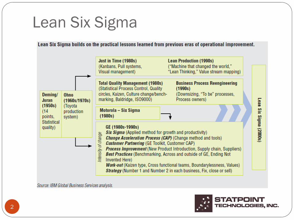
Lean Six Sigma
2
Lean Six Sigma
3
Lean manufacturing – focuses on reducing cost through
process optimization.
Six Sigma – focuses on meeting customer requirements and
stakeholder expectations, and improving quality by
measuring and eliminating defects.
www-935.ibm.com/services/uk/bcs/pdf
/driving_operational_innovation_using_lean_six_sigma.pdf
Statgraphics Software
4
Statgraphics Centurion XVI.I –Windows standalone application
with over 170 basic and advanced statistical methods.
Statgraphics Sigma Express 1.1 – Excel add-in with 70+
procedures covering the needs of Six Sigma green belts and
most black belts. Available for Excel 2003, 2007, 2010.*
*Pre-release evaluation version available by sending contact information to
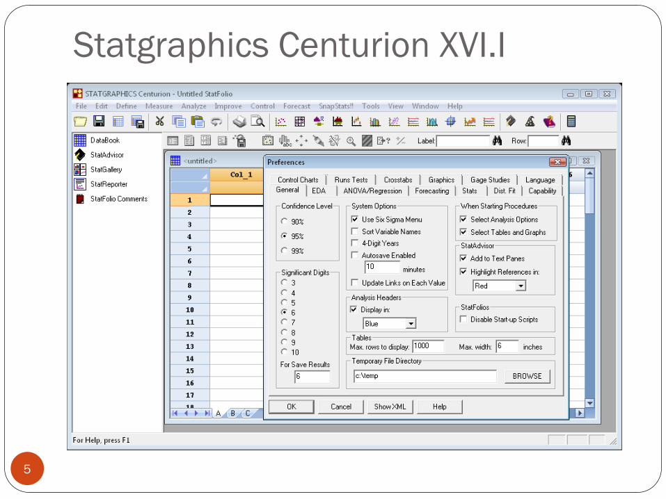
Statgraphics Centurion XVI.I
5

Statgraphics Sigma Express
6

Example #1 (Define) –
Cause-and-Effect Diagram
7
Cause-and-effect diagrams (also called fishbone or Ishikawa diagrams)
illustrate the causes of specific events.
Event: defects
Major causes: material, personnel, environment, machines, …

Input – Analysis Options dialog box
creates diagram
8
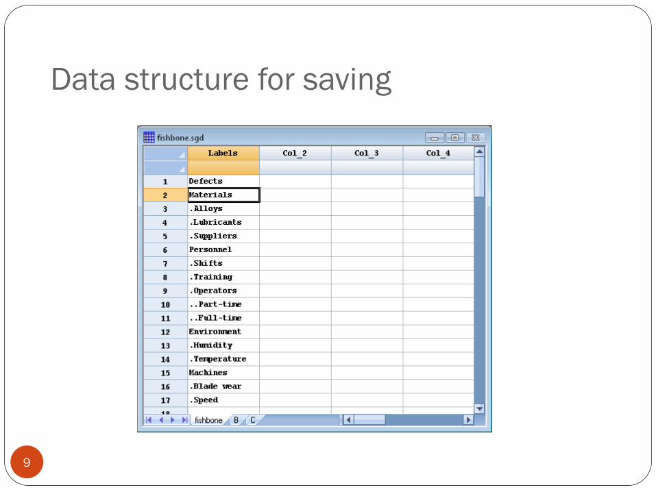
Data structure for saving
9
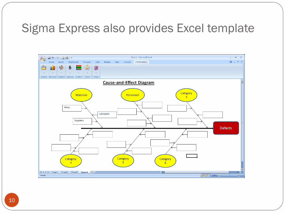
Sigma Express also provides Excel template
10
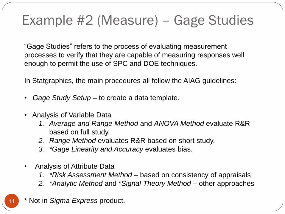
Example #2 (Measure) – Gage Studies
11
“Gage Studies” refers to the process of evaluating measurement
processes to verify that they are capable of measuring responses well
enough to permit the use of SPC and DOE techniques.
In Statgraphics, the main procedures all follow the AIAG guidelines:
• Gage Study Setup – to create a data template.
• Analysis of Variable Data
1. Average and Range Method and ANOVA Method evaluate R&R
based on full study.
2. Range Method evaluates R&R based on short study.
3. *Gage Linearity and Accuracy evaluates bias.
• Analysis of Attribute Data
1. *Risk Assessment Method – based on consistency of appraisals
2. *Analytic Method and *Signal Theory Method – other approaches
* Not in Sigma Express product.

Statistical Model
12
2
.
2
processtmeasuremenproducttotal
22
. ilityreproducibityrepeatabilprocesstmeasuremen
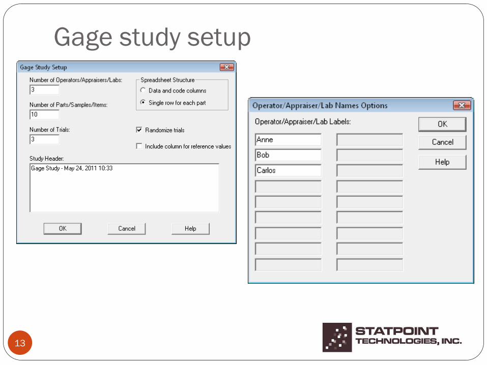
Gage study setup
13
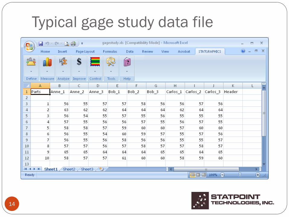
Typical gage study data file
14
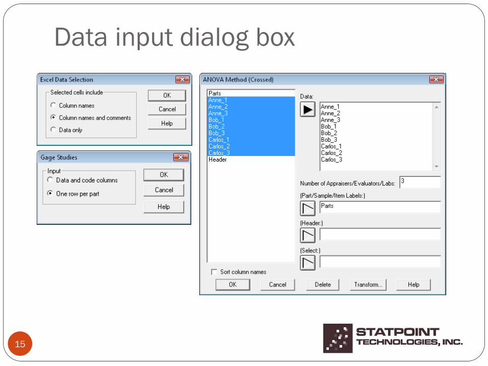
Data input dialog box
15
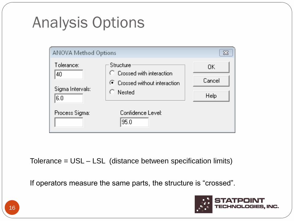
Analysis Options
16
Tolerance = USL – LSL (distance between specification limits)
If operators measure the same parts, the structure is “crossed”.
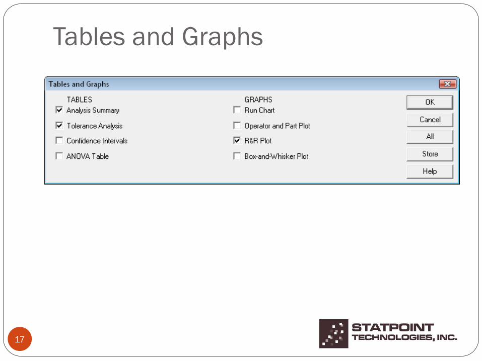
Tables and Graphs
17
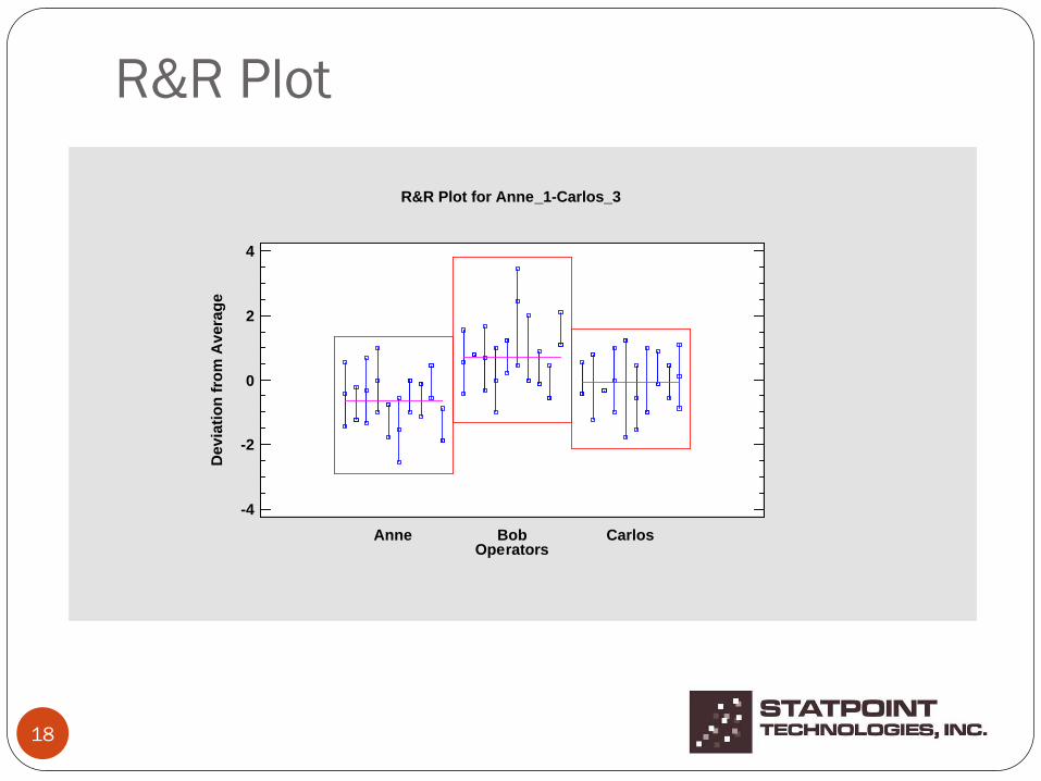
R&R Plot
18
R&R Plot for Anne_1-Carlos_3
Operators
-4
-2
0
2
4
Devia
tio
n f
rom
Avera
ge
Anne Bob Carlos
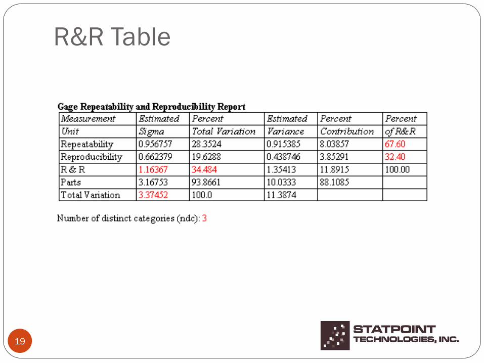
R&R Table
19

Tolerance Analysis
20
%ˆ6
100.
tolerance
processtmeasuremen
Precision-to-tolerance ratio:
Example #3 (Analyze) – Capability Analysis
21
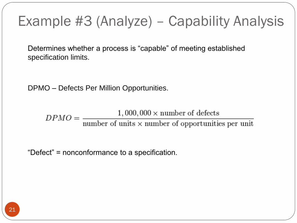
Determines whether a process is “capable” of meeting established
specification limits.
DPMO – Defects Per Million Opportunities.
“Defect” = nonconformance to a specification.
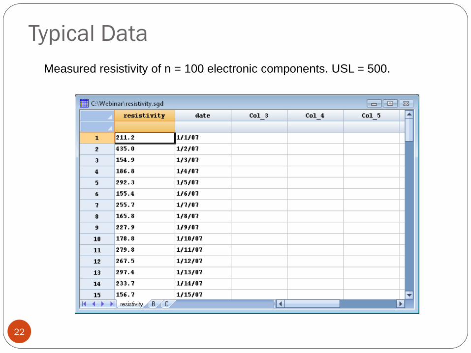
Typical Data
22
Measured resistivity of n = 100 electronic components. USL = 500.
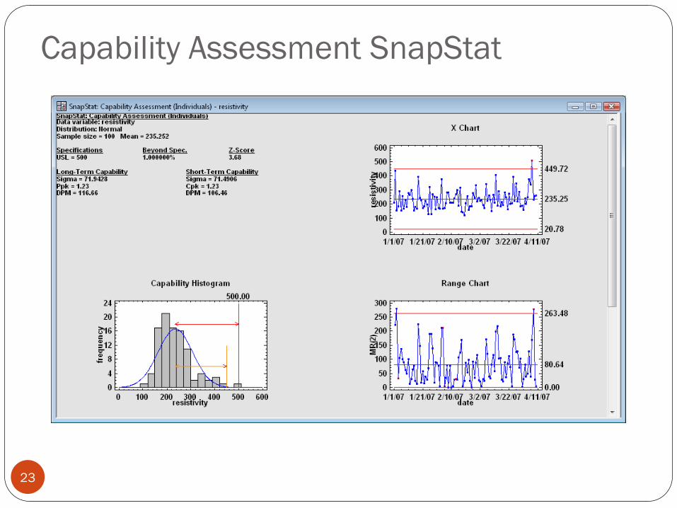
Capability Assessment SnapStat
23
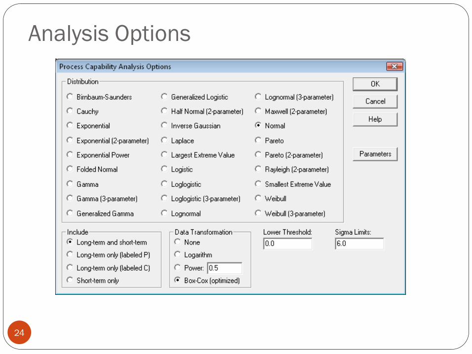
Analysis Options
24
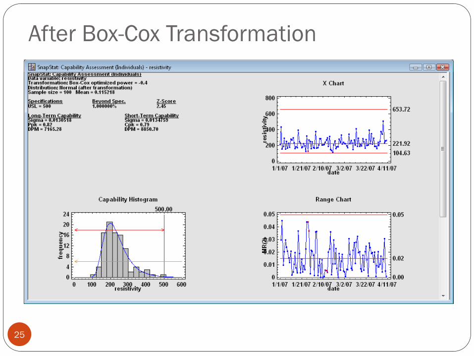
After Box-Cox Transformation
25
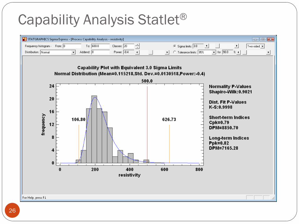
Capability Analysis Statlet®
26
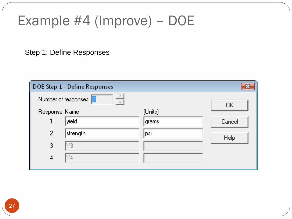
Example #4 (Improve) – DOE
27
Step 1: Define Responses
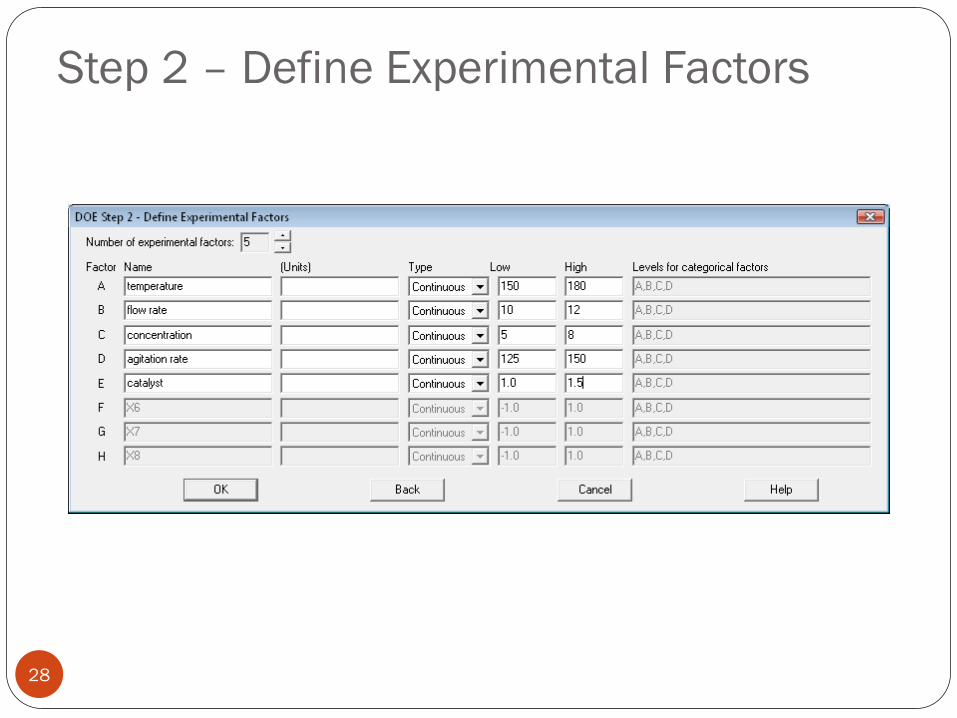
Step 2 – Define Experimental Factors
28
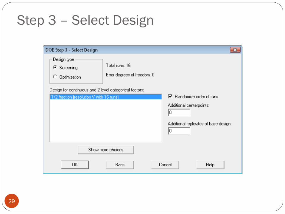
Step 3 – Select Design
29

Step 4 – Paste to Excel Worksheet
30
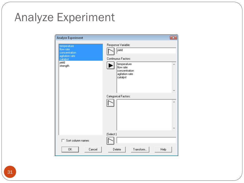
Analyze Experiment
31
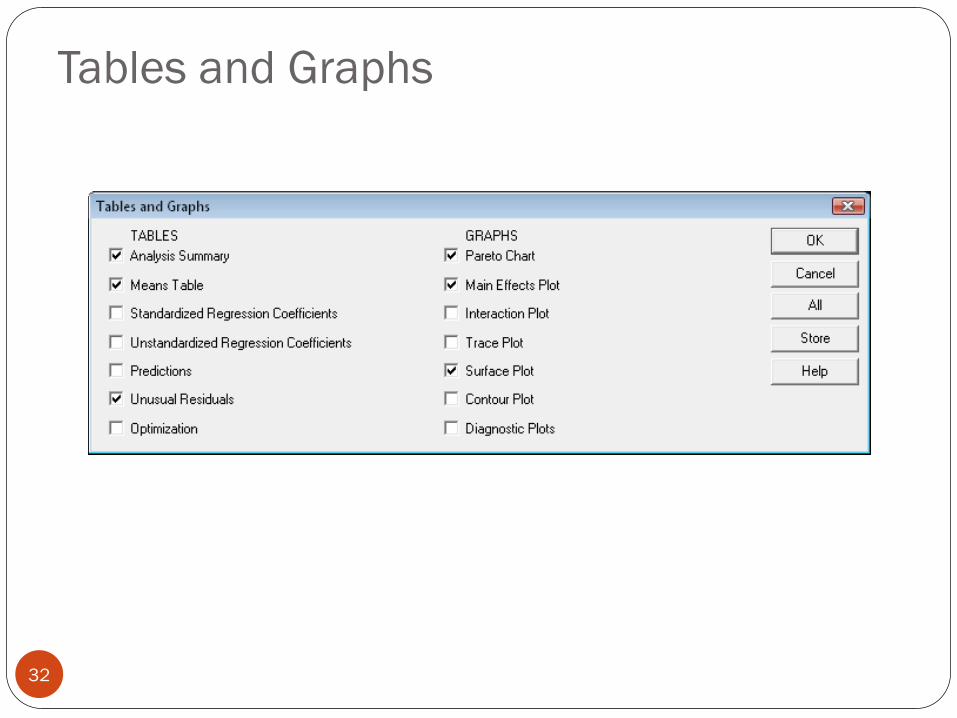
Tables and Graphs
32

Analysis Window
33
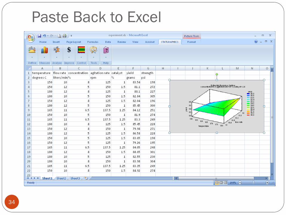
Paste Back to Excel
34
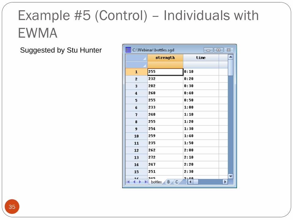
Example #5 (Control) – Individuals with
EWMA
35
Suggested by Stu Hunter
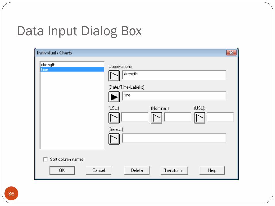
Data Input Dialog Box
36
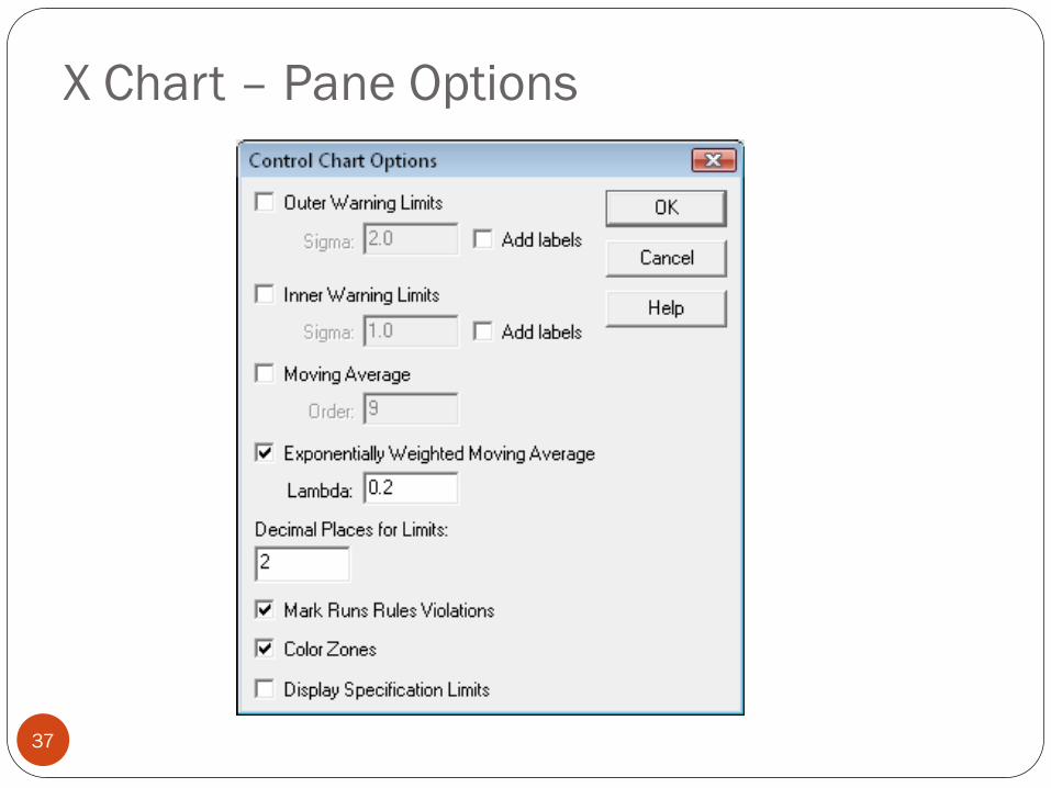
X Chart – Pane Options
37
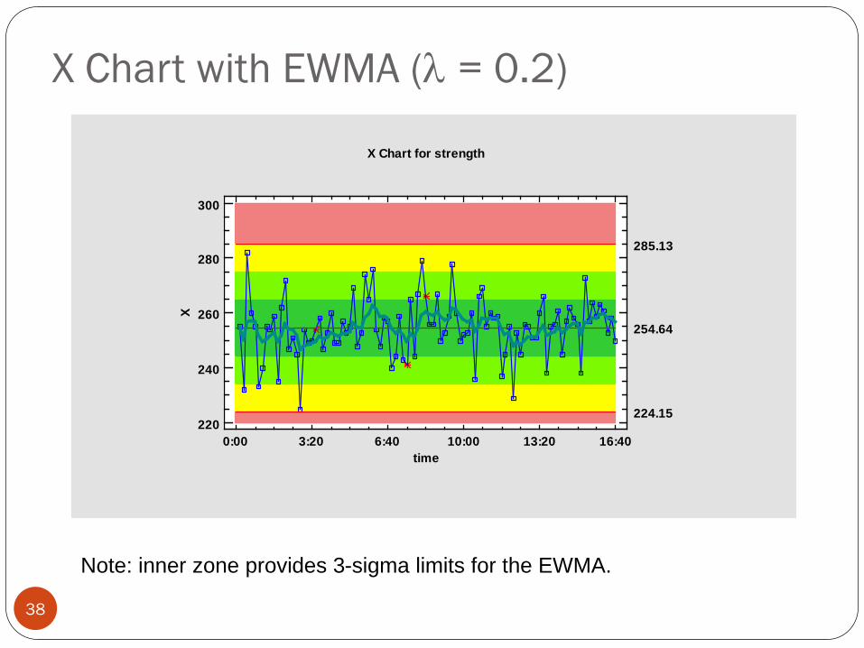
X Chart with EWMA (l = 0.2)
38
285.13
X Chart for strength
0:00 3:20 6:40 10:00 13:20 16:40
time
220
240
260
280
300
X
254.64
224.15
Note: inner zone provides 3-sigma limits for the EWMA.
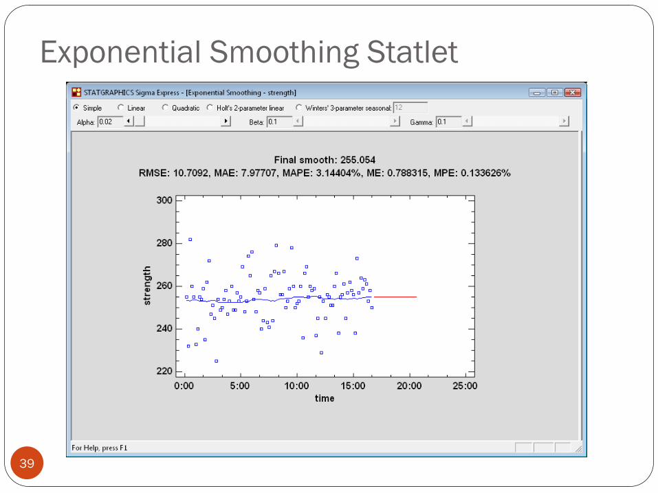
Exponential Smoothing Statlet
39

Example #6 - Monte Carlo Simulation
40
Step 1
Normal (12.1, 1.9)
Step 2
Normal (7.3, 0.5)
Step 3
Exponential (0.2)
Step 4
Uniform (2.0, 6.0)
Cycle time = Step 1 + Step 2 + MAX(Step 3, Step 4)
Cycle
time
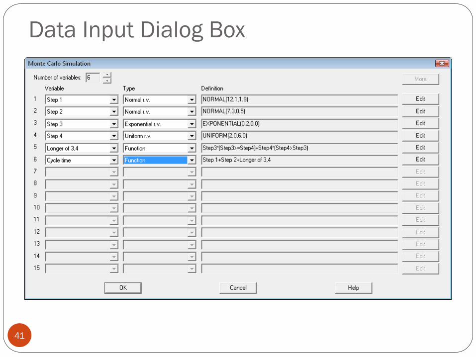
Data Input Dialog Box
41
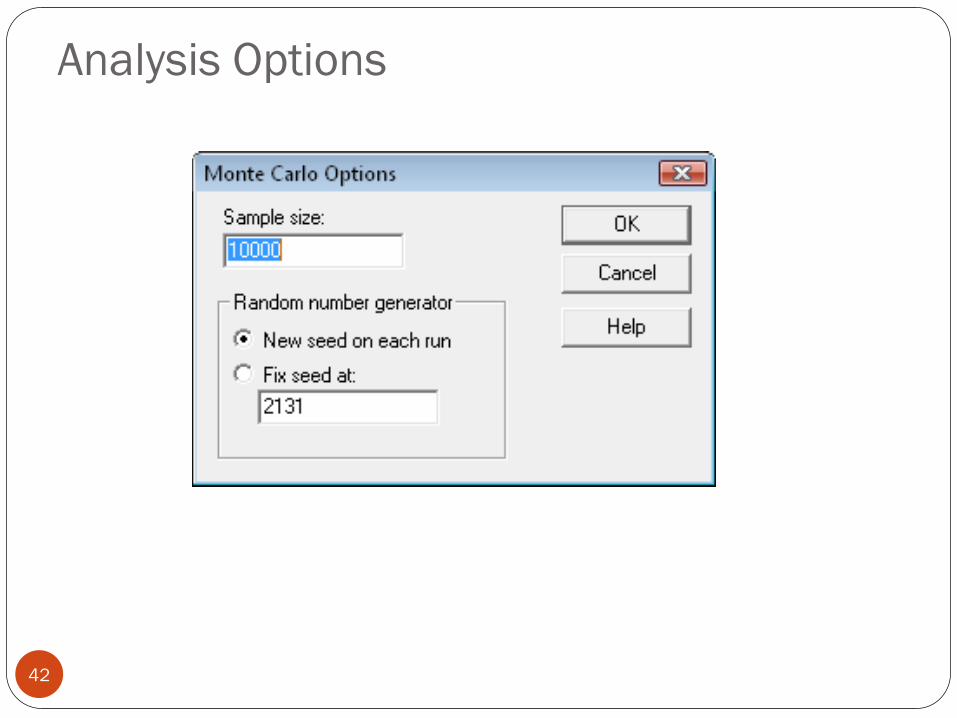
Analysis Options
42
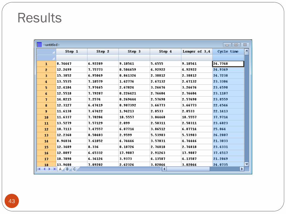
Results
43
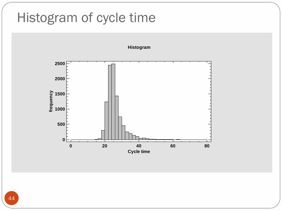
Histogram of cycle time
44
Histogram
0 20 40 60 80
Cycle time
0
500
1000
1500
2000
2500
fre
qu
en
cy