WP/04/234

Technology Shocks and Aggregate Fluctuations: How Well Does the Real Business Cycle Model Fit

Postwar U.S. Data?

Jordi Galí and Pau Rabanal

© 2004 International Monetary Fund WP/04/234

IMF Working Paper

Western Hemisphere Department

Technology Shocks and Aggregate Fluctuations: How Well Does the Real Business Cycle Model Fit Postwar U.S. Data?

Prepared by Jordi Galí and Pau Rabanal1

Authorized for distribution by Tamim Bayoumi

December 2004

Abstract

This Working Paper should not be reported as representing the views of the IMF. The views expressed in this Working Paper are those of the author(s) and do not necessarily represent those of the IMF or IMF policy. Working Papers describe research in progress by the author(s) and are published to elicit comments and to further debate.

Our answer: Not so well. We reached that conclusion after reviewing recent research on the role of technology as a source of economic fluctuations. The bulk of the evidence suggests a limited role for aggregate technology shocks, pointing instead to demand factors as the main force behind the strong positive comovement between output and labor input measures. JEL Classification Numbers: E32 Keywords: Real Business Cycles, Technology Shocks, Nominal Rigidities, Real Frictions Author(s) E-Mail Address: jordi.gali@upf.edu, prabanal@imf.org

1 Prepared for the 19th NBER Annual Conference on Macroeconomics. We are thankful to Susanto Basu, Olivier Blanchard, Yongsung Chang, John Fernald, Albert Marcet, Barbara Rossi, Julio Rotemberg, Juan Rubio-Ramirez, Robert Solow, Jaume Ventura, Lutz Weinke, as well as the editors, Mark Gertler and Ken Rogoff, and discussants, Ellen McGrattan and Valerie Ramey, for useful comments. We have also benefited from comments by participants in seminars at the CREI-UPF Macro Workshop, MIT Macro Faculty Lunch, and Duke University. Anton Nakov provided excellent research assistance. We are grateful to Craig Burnside, Ellen McGrattan, Harald Uhlig, Jonas Fisher, and Susanto Basu for help with the data. Galí acknowledges financial support from DURSI (Generalitat de Catalunya), Fundación Ramón Areces, and the Ministerio de Ciencia y Tecnología (SEC2002–03816).

- 2 -

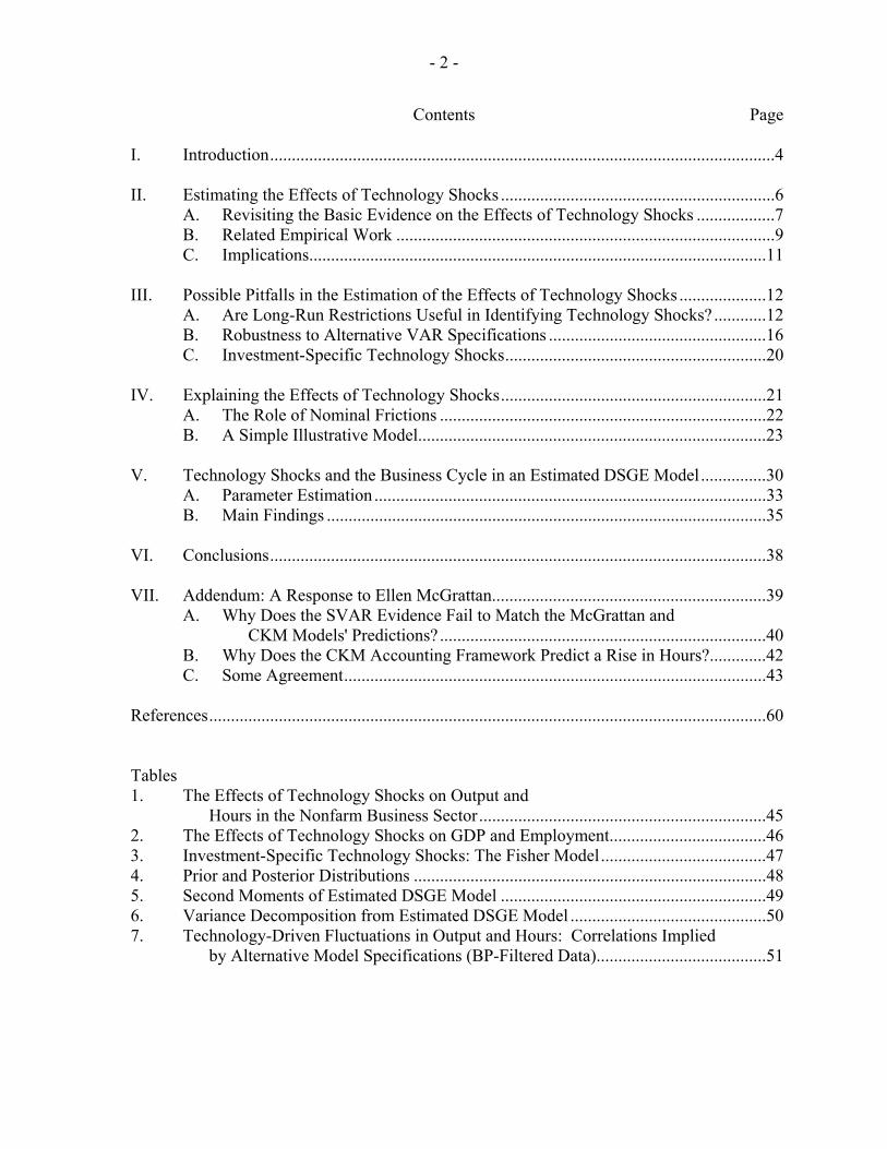
Contents Page I. Introduction....................................................................................................................4 II. Estimating the Effects of Technology Shocks ...............................................................6 A. Revisiting the Basic Evidence on the Effects of Technology Shocks ..................7 B. Related Empirical Work .......................................................................................9 C. Implications.........................................................................................................11 III. Possible Pitfalls in the Estimation of the Effects of Technology Shocks ....................12 A. Are Long-Run Restrictions Useful in Identifying Technology Shocks? ............12 B. Robustness to Alternative VAR Specifications ..................................................16 C. Investment-Specific Technology Shocks............................................................20 IV. Explaining the Effects of Technology Shocks.............................................................21 A. The Role of Nominal Frictions ...........................................................................22 B. A Simple Illustrative Model................................................................................23 V. Technology Shocks and the Business Cycle in an Estimated DSGE Model...............30 A. Parameter Estimation ..........................................................................................33 B. Main Findings .....................................................................................................35 VI. Conclusions..................................................................................................................38 VII. Addendum: A Response to Ellen McGrattan...............................................................39 A. Why Does the SVAR Evidence Fail to Match the McGrattan and CKM Models' Predictions?...........................................................................40 B. Why Does the CKM Accounting Framework Predict a Rise in Hours?.............42 C. Some Agreement.................................................................................................43 References................................................................................................................................60 Tables 1. The Effects of Technology Shocks on Output and Hours in the Nonfarm Business Sector..................................................................45 2. The Effects of Technology Shocks on GDP and Employment....................................46 3. Investment-Specific Technology Shocks: The Fisher Model......................................47 4. Prior and Posterior Distributions .................................................................................48 5. Second Moments of Estimated DSGE Model .............................................................49 6. Variance Decomposition from Estimated DSGE Model .............................................50 7. Technology-Driven Fluctuations in Output and Hours: Correlations Implied by Alternative Model Specifications (BP-Filtered Data).......................................51

- 3 - Figures 1. Business Cycle Fluctuations in Output and Hours.......................................................52 2. The Estimated Effects of Technology Shocks (Difference specification, sample period 1948:01–2002:04)...........................................................................533. Sources of Business Cycle Fluctuations, (Difference specification, sample period 1948:01–2002:04) ..........................................................................54 4. Capital Income Tax Rates............................................................................................55 5. Technology Shocks: VAR versus BFK .......................................................................56 6. Hours Worked (In natural logarithms, 1948–2002).....................................................57 7. Posterior Impulse Responses to a Technology Shock, Estimated DSGE Model ........58 8. The Role of Technology Shocks in U.S. Postwar Fluctuations: Model-Based Estimates .........................................................................................59

- 4 -

I. INTRODUCTION

Since the seminal work of Kydland and Prescott (1982) and Prescott (1986a) proponents of the Real Business Cycle (RBC) paradigm have claimed a central role for exogenous variations in technology as a source of economic fluctuations in industrial economies. Those fluctuations have been interpreted by RBC economists as the equilibrium response to exogenous variations in technology, in an environment with perfect competition and intertemporally optimizing agents, and in which the role of nominal frictions and monetary policy is, at most, secondary. Behind the claims of RBC theory lies what must have been one of the most revolutionary findings in postwar macroeconomics: a calibrated version of the neoclassical growth model augmented with a consumption-leisure choice, and with stochastic changes in total factor productivity as the only driving force, seems to account for the bulk of economic fluctuations in the postwar U.S. economy. In practice, “accounting for observed fluctuations” has meant that calibrated RBC models match pretty well the patterns of unconditional second moments of a number of macroeconomic time series, including their relative standard deviations and correlations. Such findings led Prescott to claim “...that technology shocks account for more than half the fluctuations in the postwar period, with a best point estimate near 75 percent.”2 Similarly, in two recent assessments of the road traveled and the lessons learned by RBC theory after more than a decade, Cooley and Prescott (1995) could confidently claim that “it makes sense to think of fluctuations as caused by shocks to productivity,” while King and Rebelo (1999) concluded that “...[the] main criticisms levied against first-generation real business cycle models have been largely overcome.” While most macroeconomists have recognized the methodological impact of the RBC research program and have adopted its modeling tools, other important, more substantive elements of that program have been challenged in recent years. First, and in accordance with the widely acknowledged importance of monetary policy in industrial economies, the bulk of the profession has gradually moved away from real models (or their near-equivalent frictionless monetary models) when trying to understand short-run macroeconomic phenomena. Second, and most important for the purposes of this paper, the view of technological change as a central force behind cyclical fluctuations has been called into question. In the present paper we focus on the latter development, by providing an overview of the literature that has challenged the central role of technology in business cycles. A defining feature of the literature reviewed here lies in its search for evidence on the role of technology that is “more direct” than just checking whether any given model driven by technology shocks, and more or less plausibly calibrated, can generate the key features of the business cycle. In particular, we discuss efforts to identify and estimate the empirical effects of exogenous changes in technology on different macroeconomic variables, and to evaluate quantitatively the contribution of those changes to business cycle fluctuations. 2 Prescott (1986b).

- 5 -

Much of that literature (and, hence, much of the present paper) focuses on one central, uncontroversial feature of the business cycle in industrial economies—namely, the strong positive comovement between output and labor input measures. That comovement is illustrated graphically in Figure 1, which displays the quarterly time series for hours and output in the U.S. nonfarm business sector over the period 1948:1-2002:4. In both cases the original series have been transformed using the band-pass filter developed in Baxter and King (1999), calibrated to remove fluctuations of periodicity outside an interval between 6 and 32 quarters. As in Stock and Watson (1999), we interpret the resulting series as reflecting fluctuations associated with business cycles. As is well known, the basic RBC model can generate fluctuations in labor input and output of magnitude, persistence, and degree of comovement roughly similar to the series displayed in Figure 1. Furthermore, and as shown in King and Rebelo (1999), when the actual sequence of technology shocks (proxied by the estimated disturbances of an AR process for the Solow residual) is fed as an input into the model, the resulting equilibrium paths of output and labor input track surprisingly well the observed historical patterns of those variables; the latter exercise can be viewed as a more stringent test of the RBC model than the usual moment-matching. The literature reviewed in the present paper asks, however, very different questions: What have been the effects of technology shocks in the postwar U.S. economy? How do they differ from the predictions of standard RBC models? What is their contribution to business cycle fluctuations? What features must be incorporated in business cycle models to account for the observed effects? The remainder of this paper describes the tentative (and sometimes contradictory) answers that the efforts of a growing number of researchers have yielded. Some of that research has exploited the natural role of technological change as a source of permanent changes in labor productivity to identify technology shocks using structural vector autorregressions (VARs); other authors have instead relied on more direct measures of technological change and examined their comovements with a variety of macro variables. It is not easy to summarize in a few words the wealth of existing evidence nor to agree on some definite conclusions of a literature that is still very much ongoing. Nevertheless, it is safe to state that the bulk of the evidence reviewed in the present paper provides little support for the initial claims of the RBC literature on the central role of technological change as a source of business cycles. The remainder of the paper is organized as follows. Section II reviews some of the early papers that questioned the importance of technology shocks, and presents some of the basic evidence regarding the effects of those shocks. Section III discusses a number of criticisms and possible pitfalls of that literature. Section IV presents the case for the existence of nominal frictions as an explanation of the estimated effects of technology shocks, and summarizes some of the real explanations for the same effects found in the literature. Section V lays out and analyzes an estimated dynamic stochastic general equilibrium (DSGE) model that incorporates both nominal and real frictions, and evaluates their respective role. Section VI concludes.

- 6 -

II. ESTIMATING THE EFFECTS OF TECHNOLOGY SHOCKS

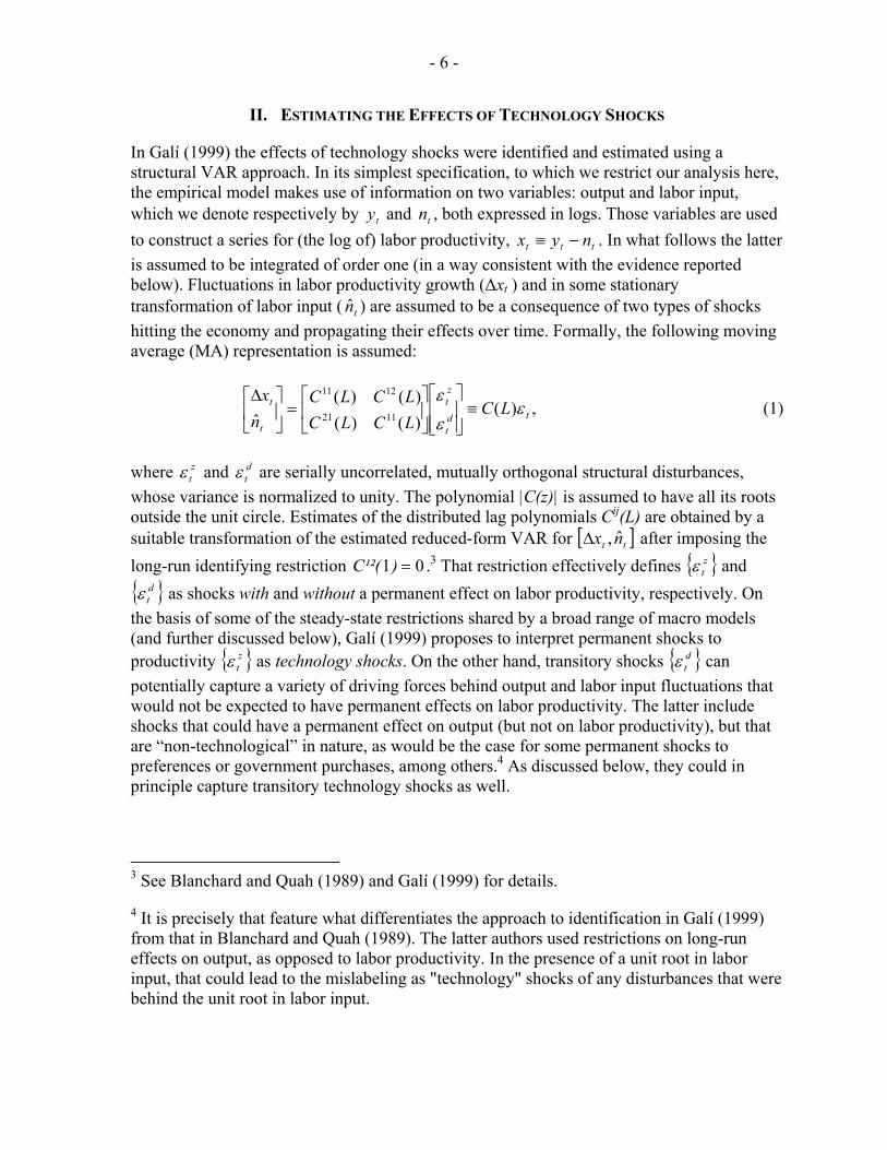
In Galí (1999) the effects of technology shocks were identified and estimated using a structural VAR approach. In its simplest specification, to which we restrict our analysis here, the empirical model makes use of information on two variables: output and labor input, which we denote respectively by ty and tn , both expressed in logs. Those variables are used to construct a series for (the log of) labor productivity, ttt nyx −≡ . In what follows the latter is assumed to be integrated of order one (in a way consistent with the evidence reported below). Fluctuations in labor productivity growth (∆xt ) and in some stationary transformation of labor input ( tn̂ ) are assumed to be a consequence of two types of shocks hitting the economy and propagating their effects over time. Formally, the following moving average (MA) representation is assumed:

,)()()()()(

ˆ 1121

1211

tdt

zt

t

t LCLCLCLCLC

nx

εε

ε≡

⎥⎥⎦

⎤

⎢⎢⎣

⎡⎥⎦

⎤⎢⎣

⎡=⎥

⎦

⎤⎢⎣

⎡∆ (1)

where z

tε and dtε are serially uncorrelated, mutually orthogonal structural disturbances,

whose variance is normalized to unity. The polynomial |C(z)| is assumed to have all its roots outside the unit circle. Estimates of the distributed lag polynomials Cij(L) are obtained by a suitable transformation of the estimated reduced-form VAR for [ ]tt nx ˆ,∆ after imposing the long-run identifying restriction 01 =)C¹²( .3 That restriction effectively defines { }z

tε and { }d

tε as shocks with and without a permanent effect on labor productivity, respectively. On the basis of some of the steady-state restrictions shared by a broad range of macro models (and further discussed below), Galí (1999) proposes to interpret permanent shocks to productivity { }z

tε as technology shocks. On the other hand, transitory shocks { }dtε can

potentially capture a variety of driving forces behind output and labor input fluctuations that would not be expected to have permanent effects on labor productivity. The latter include shocks that could have a permanent effect on output (but not on labor productivity), but that are “non-technological” in nature, as would be the case for some permanent shocks to preferences or government purchases, among others.4 As discussed below, they could in principle capture transitory technology shocks as well.

3 See Blanchard and Quah (1989) and Galí (1999) for details.

4 It is precisely that feature what differentiates the approach to identification in Galí (1999) from that in Blanchard and Quah (1989). The latter authors used restrictions on long-run effects on output, as opposed to labor productivity. In the presence of a unit root in labor input, that could lead to the mislabeling as "technology" shocks of any disturbances that were behind the unit root in labor input.

- 7 -

A. Revisiting the Basic Evidence on the Effects of Technology Shocks

Next, we revisit and update the basic evidence on the effects of technology shocks reported in Galí (1999). Our baseline empirical analysis uses quarterly U.S. data for the period 1948:1-2002:4. Our source is the Haver USECON database, for which we list the associated mnemonics. Our series for output corresponds to nonfarm business sector output (LXNFO). Our baseline labor input series is hours of all persons in the nonfarm business sector (LXNFH). Below we often express the output and hours series in per capita terms, using a measure of civilian noninstitutional population aged 16 and over (LNN). Our baseline estimates are based on a specification of hours in first-differences -i.e., we set

tt nn ∆=ˆ . That choice seems consistent with the outcome of Augmented Dickey-Fuller (ADF) tests applied to the hours series, which do not reject the null of a unit root in the level of hours at a 10 percent significance level, against the alternative of stationarity around a linear deterministic trend. On the other hand, the null of a unit root in the first-differenced series is rejected at a level of less than 1 percent.5 In a way consistent with the previous result, a Kwiatkowski et al. (1992) (KPSS) test applied to tn rejects the stationarity null with a significance level below 1 percent, while failing to reject the same null when applied to

tn∆ . In addition, the same battery of ADF and KPSS tests applied to our tx and tx∆ series support the existence of a unit root in labor productivity, a necessary condition for the identification strategy based on long-run restrictions employed here. Both observations suggest the specification and estimation of a VAR for [ ]tt nx ∆∆ , . Henceforth, we refer to the latter as the difference specification. Figure 2 displays the estimated effects of a positive technology shock, of size normalized to one standard deviation. The graphs on the left show the dynamic responses of labor productivity, output, and hours, together with (±) two standard error bands.6 The corresponding graphs on the right show the simulated distribution of each variable’s response on impact. As in Galí (1999), the estimates point to a significant and persistent decline in hours after a technology shock that raises labor productivity permanently.7 The point estimates suggest that hours do eventually return to their original level (or close to it), but not until more than a year later. Along with that pattern of hours, we observe a positive but muted initial response of output in the face of a positive technology shock.

5 With four lags, the corresponding t-statistics are -2.5 and -7.08 for the level and the first-difference, respectively.

6 That distribution is obtained by means of a Montecarlo simulation based on 500 drawings from the distribution of the reduced-form VAR distribution.

7 Notice that the distribution of the impact effect on hours assigns a zero probability to an increase in that variable.

- 8 -

The estimated responses to a technology shock displayed in Figure 2 contrast starkly with the predictions of a standard calibrated RBC model, which would predict a positive comovement among the three variables plotted in the figure in response to that shock.8 Not surprisingly, the previous estimates have dramatic implications regarding the sources of the business cycle fluctuations in output and hours displayed in Figure 1. This is illustrated in Figure 3, which displays the estimated business cycle components of the historical series for output and hours associated with technology and non-technology shocks. In both cases the estimated components of the (log) levels of productivity and hours have been detrended using the same band-pass filter underlying the series plotted in Figure 1. As in Galí (1999), the picture that emerges is very clear: fluctuations in hours and output driven by technology shocks account for a small fraction of the variance of those variables at business cycle frequencies: 5 and 7 percent, respectively. Furthermore, the comovement at business cycle frequencies between output and hours resulting from technology shocks is shown to be essentially zero (the correlation is -0.08), in contrast with the high positive comovement observed in the data (0.88). Clearly, the pattern of technology-driven fluctuations, as identified in our structural VAR, shows little resemblance with the conventional business cycle fluctuations displayed in Figure 1. The picture changes dramatically if we turn our attention to the estimated fluctuations of output and hours driven by shocks with no permanent effects on productivity (displayed in the bottom graph). Those shocks account for 95 and 93 percent of the variance of the business cycle component of hours and output, respectively. In addition, they generate a nearly perfect correlation (0.96) between the same variables. In contrast with its technology-driven counterpart, this component of output and hours fluctuations displays a far more recognizable business cycle pattern. A possible criticism to the above empirical framework is the assumption of only two driving forces underlying the fluctuations in hours and labor productivity. As discussed in Blanchard and Quah (1989), ignoring some relevant shocks may lead to a significant distortion in the estimated impulse responses. Galí (1999) addresses that issue by estimating a five-variable VAR (including time series on real balances, interest rates, and inflation). That framework allows for as many as four shocks with no permanent effects on productivity, and for which no separate identification is attempted. The estimates generated by that higher-dimensional model regarding the effects of technology shocks are very similar to the ones reported above, suggesting that the focus on two shocks only may not be restrictive for the issue at hand.9

8 See, e.g., King, Plosser, and Rebelo (1988a) and Campbell (1994).

9 See also Francis and Ramey (2003a), among others, for estimates using higher dimensional VARs.

- 9 -

B. Related Empirical Work

The empirical connection between technological change and business cycle fluctuations has been the focus of a rapidly expanding literature. Next we briefly discuss some recent papers providing evidence on the effects of technology shocks, and that reach conclusions similar to those in Galí (1999), while using a different data set or empirical approach. We leave for later a discussion of the papers whose findings relate more specifically to the content of other sections, including those that question the evidence reported above. An early contribution is given by the relatively unknown paper by Blanchard, Solow and Wilson (1995). That paper already spells out some of the key arguments found in the subsequent literature. In particular, it stresses the need to sort out the component of productivity associated with exogenous technological change from the component that varies in response to other shocks that may affect the capital-labor ratio. They adopt a simple instrumental variables approach, with a number of demand-side variables assumed to be orthogonal to exogenous technological change used as instruments for employment growth or the change in unemployment in a regression that features productivity growth as a dependent variable. The fitted residual in that regression is interpreted as a proxy for technology-driven changes in productivity. When they regress the change in unemployment on the filtered productivity growth variable they obtain a positive coefficient—i.e. an (exogenous) increase in productivity drives the unemployment rate up. A dynamic specification of that regression implies that such an effect lasts for about three quarters, after which unemployment starts to fall and returns rapidly to its original value. As mentioned in Galí (1999, footnote 19) and stressed by Valerie Ramey in her discussion, the finding of a decline in hours (or an increase in unemployment) in response to a positive technology shock could also have been detected by an attentive reader in a number of earlier VAR papers, though that finding generally goes unnoticed or is described as puzzling. Blanchard and Quah (1989) and Blanchard (1989) are exceptions in that they provide some explicit discussion of the finding, which they interpret as consistent with a traditional Keynesian model “in which increases in productivity...may well increase unemployment in the short run if aggregate demand does not increase enough to maintain employment”.10 The work of Basu, Fernald, and Kimball (1999; henceforth, BFK) deserves special attention here, given its focus and the similarity of its findings to those in Galí (1999) despite the use of an unrelated methodology. BFK use a sophisticated growth accounting methodology allowing for increasing returns, imperfect competition, variable factor utilization and sectoral compositional effects in order to uncover a time series for aggregate technological change in the postwar U.S. economy. Their approach, combining elements of earlier work by Hall (1988) and Basu and Kimball (1997) among others, can be viewed as an attempt to cleanse the Solow residual (Solow, 1957) of its widely acknowledged measurement error resulting from the strong assumptions underlying its derivation. Estimates of the response of the economy to innovations in their measure of technological change point to a sharp short-run 10 Blanchard (1989, p. 1158).

- 10 -

decline in the use of inputs (including labor) when technology improves, with output showing no significant change (with point estimates suggesting a small decline). After that short-run impact both variables gradually adjust upward, with labor input returning to its original level and with output reaching a permanently higher plateau several years after the shock. Kiley (1997) applies the structural VAR framework in Galí (1999) to data from two-digit manufacturing industries. While he does not report impulse responses, he finds that technology shocks induce a negative correlation between employment and output growth in 12 of the 17 industries considered. When he estimates an analogous conditional correlation for employment and productivity growth, he obtains a negative value for 15 out of 17 industries. Francis (2001) conducts a similar analysis, though he attempts to identify industry-specific technology shocks by including a measure of aggregate technology, which is assumed to be exogenous to each of the industries considered. He finds that, for the vast majority of industries, a sectoral labor input measure declines in response to a positive industry-specific technology shock. Using data from a large panel of 458 manufacturing industries and 35 sectors, Franco and Philippon (2004) estimate a structural VAR with three shocks: technology shocks (with permanent effects on industry productivity), composition shocks (with permanent effects on the industry share in total output), and transitory shocks. They find that technology shocks (i) generate a negative comovement between output and hours within each industry, and (ii) are almost uncorrelated across industries. Accordingly, they conclude that technology shocks can only account for a small fraction of the variance of aggregate hours and output (with two-thirds of the latter accounted for by transitory shocks). Shea (1998) uses a structural VAR approach to model the connection between changes in measures of technological innovation (research and development (R&D) and number of patent applications) and subsequent changes in total factor productivity (TFP) and hired inputs, using industry-level data. For most specifications and industries he finds that an innovation in the technology indicator does not cause any significant change in TFP, but tends to increase labor inputs in the short run. While not much stressed by Shea, however, one of the findings in his paper is particularly relevant for our purposes: in the few VAR specifications for which a significant increase in TFP is detected in response to a positive innovation in the technology indicator, inputs—including labor—are shown to respond in the direction opposite to the movement in TFP, a finding in line with the evidence above.11 Francis and Ramey (2003a) extend the analysis in Galí (1999) in several dimensions. The first modification they consider consists in augmenting the baseline VAR (specified in first differences) with a capital tax rate measure in order to sort out the effects of technology shocks from those of permanent changes in tax rates (more below). Second, they identify technology shocks as those with permanent effects on real wages (as opposed to labor productivity) and/or no long-run effects on hours, both equally robust predictions of a broad class of models that satisfy a balance growth property. Those alternative identifying 11 See the comment on Shea's paper by Galí (1998) for a more detailed discussion of that point.

- 11 -

restrictions are not rejected when combined into a unified (overidentified) model. Francis and Ramey show that both the model augmented with capital tax rates and the model with alternative identifying restrictions (considered separately or jointly) imply impulse responses to a technology shock similar to those in Galí (1999) and, in particular, a drop in hours in response to a positive technology shock. Francis, Owyang, and Theodorou (2003) use a variant of the sign restriction algorithm of Uhlig (1999) and show that the finding of a negative response of hours to a positive technology shock is robust to replacing the restriction on the asymptotic effect of that shock with one imposing a positive response of productivity at a horizon of ten years after the shock. A number of recent papers have provided related evidence based on non-U.S. aggregate data. In Galí (1999) the structural VAR framework discussed above is also applied to the remaining G-7 countries (Canada, the United Kingdom, France, Germany, Italy, and Japan). He uncovers a negative response of employment to a positive technology shock in all countries, with the exception of Japan. Galí (1999) also points out some differences in these estimates relative to those obtained for the United States: in particular, the (negative) employment response to a positive technology shocks in Germany, the United Kingdom, and Italy appears to be larger and more persistent, which could be interpreted as evidence of "hysteresis" in European labor markets. Very similar qualitative results for the euro area as a whole can also be found in Galí (2004), which applies the same empirical framework to the quarterly data set that has recently become available. In particular, technology shocks are found to account for only 5 percent and 9 percent of the variance of the business cycle component of euro-area employment and output, respectively, with the corresponding correlation between their technology-driven components being -0.67. Francis and Ramey (2003b) estimate a structural VAR with long-run identifying restrictions using long-term U.K. annual time series tracing back to the nineteenth century; they find robust evidence of a negative short-run impact of technology shocks on labor in every subsample.12 Finally, Carlsson (2000) develops a variant of the empirical framework in BFK (1999) and Burnside, Eichenbaum, and Rebelo (1995) to construct a time series for technological change, and applies it to a sample of Swedish two-digit manufacturing industries. Most prominently, he finds that positive shocks to technology have, on impact, a contractionary effect on hours and a non-expansionary effect on output, as in BFK (1999).

C. Implications

The implications of the evidence discussed above for business cycle analysis and modeling are manifold. Most significantly, those findings reject a key prediction of the standard RBC paradigm—namely, the positive comovement of output, labor input, and productivity in response to technology shocks. That positive comovement is the single main feature of that 12 The latter evidence contrasts with their analysis of long-term U.S. data, in which the results vary significantly across samples and appear to depend on the specification used (more below).

- 12 -

model that accounts for its ability to generate fluctuations that resemble business cycles. Hence, taken at face value, the evidence above rejects in an unambiguous fashion the empirical relevance of the standard RBC model. It does so in two dimensions. First, it shows that a key feature of the economy's response to aggregate technology shocks predicted by calibrated RBC models cannot be found in the data. Second, and to the extent that one takes the positive comovement between measures of output and labor input as a defining characteristic of the business cycle, it follows as a corollary that technology shocks cannot be a quantitatively important (and, even less, a dominant) source of observed aggregate fluctuations. While the latter implication is particularly damning for RBC theory, given its traditional emphasis on aggregate technology variations as a source of business cycles, its relevance is independent of one's preferred macroeconomic paradigm. III. POSSIBLE PITFALLS IN THE ESTIMATION OF THE EFFECTS OF TECHNOLOGY SHOCKS

This section has two main objectives. First, we try to address a question that is often raised regarding the empirical approach used in Galí (1999): To what extent can we be confident in the economic interpretation given to the identified shocks and, in particular, in the mapping between technology shocks and the nonstationary component of labor productivity? Below we provide some evidence that makes us feel quite comfortable about that interpretation. Second, we describe and address some of the econometric issues that Christiano, Eichenbaum, and Vigfusson (2003) have raised in a recent paper, and which focus on the appropriate specification of hours (levels or first differences). Finally, we discuss a recent paper by Fisher (2003), which distinguishes between two types of technology shocks, neutral and investment-specific.

A. Are Long-Run Restrictions Useful in Identifying Technology Shocks?

The approach to identification proposed in Galí (1999) relies on the assumption that only (permanent) technology shocks can have a permanent effect on (average) labor productivity. That assumption can be argued to hold under relatively weak conditions, satisfied by the bulk of business cycle models currently used by macroeconomists. To review the basic argument consider an economy whose technology can be described by an aggregate production function:13

),,( tttt NAKFY = (2) where Y denotes output, K is the capital stock, N is labor input, and A is an index of technology. Under the assumption that F is homogeneous of degree 1, we have

),1,( tktt

t kFANY

= (3)

13 An analogous but somewhat more detailed analysis can be found in Francis and Ramey (2003a)

- 13 -

where tt

tt NA

Kk = is the ratio of capital to labor (expressed in efficiency units). For a large

class of models characterized by an underlying balanced growth path, the marginal product of capital kF must satisfy, along that path, a condition of the form

)σγδρ)(µ1()1,()τ1( +++=− tk kF (4)

where µ is the price markup, τ is a tax on capital income, ρ is the time discount rate, δ is the depreciation rate, σ is the intertemporal elasticity of substitution, and γ is the average growth rate of (per capita) consumption and output. Under the assumption of decreasing returns to capital, it follows from equation (4) that the capital labor ratio k will be stationary (and will thus fluctuate around a constant mean) so long as all the previous parameters are constant (or stationary). In that case, equation (3) implies that only shocks that have a permanent effect on the technology parameter A can be a source of the unit root in labor productivity, thus providing the theoretical underpinning for the identification scheme in Galí (1999). How plausible are the assumptions underlying that identification scheme? Preference or technology parameters like ρ, δ, σ, and γ are generally assumed to be constant in most examples and applications found in the business cycle literature. The price markup µ is more likely to vary over time, possibly as a result of some embedded price rigidities; in the latter case, however, it is likely to remain stationary, fluctuating around its desired or optimal level. In the event that desired markups (or the preference and technology parameters listed above) displayed some nonstationarity, the latter would more likely take the form of some smooth function of time, which should be reflected in the deterministic component of labor productivity, but not in its fluctuations at cyclical frequencies.14 Finally, it is important to notice that the previous approach to identification of technology shocks requires that (i) kF be decreasing, so that k is uniquely pinned down by equation (4), and (ii) that the technology process { }tA is exogenous (at least with respect to the business cycle). The previous assumptions have been commonly adopted by business cycle modelers.15 Do capital income tax shocks explain permanent changes in labor productivity? The previous argument, however, is much less appealing when applied to the capital income tax rate. As Uhlig (2004) and others have pointed out, the assumption of a stationary capital income tax rate may be unwarranted, given the behavior of measures for that variable over

14 Of course that was also the traditional view regarding technological change, but one that was challenged by the RBC school.

15 Exceptions include stochastic versions of endogenous growth models, as in King, Plosser, and Rebelo (1988b). In those models any transitory shock can in principle have a permanent effect on the level of capital or disembodied technology and, as a result, on labor productivity.

- 14 -

the postwar period. This is illustrated graphically in Figure 4, which displays two alternative measures of the capital income tax rate in the United States. Figure 4.A displays a quarterly series for the average capital income tax rate constructed by Jones (2002) for the period 1958:1-1997:4. Figure 4.B shows an annual measure of the average marginal capital income tax rate constructed by Ellen McGrattan for the period 1958-92 that corresponds to an updated version of the one used in McGrattan (1994).16 Henceforth, we denote those series by J

tτ and Mtτ , respectively. Both series display an apparent non-stationary behavior, with

highly persistent fluctuations. This is confirmed by a battery of ADF tests, which fail to reject the null hypothesis of a unit root in both series, at conventional significance levels. Furthermore, as evidenced in Figures 4.C and 4.D, which display the same series in first differences, the presence of sizable short-run variations in those measures of capital taxes could hardly be captured by means of some deterministic or smooth function of time (their standard deviations being 0.79 percent for the quarterly Jones series, and 2.4 percent for the annual McGrattan series). In fact, in both cases the first-differenced series tτ∆ shows no significant autocorrelation, suggesting that a random walk process can approximate the pattern of capital income tax rates pretty well. The previous evidence, combined with the theoretical analysis above, points to a potential caveat in the identification approach followed in Galí (1999): the shocks with permanent effects on productivity estimated therein could be capturing the effects of permanent changes in tax rates (as opposed to those of genuine technology shocks). That “mislabeling” could potentially account for the empirical findings reported above. Francis and Ramey (2003a) attempt to overcome that potential shortcoming by augmenting the VAR with a capital tax rate variable, in addition to labor productivity and hours. As mentioned above, the introduction of the tax variable is shown not to have any significant influence on the findings: positive technology shocks still lead to short run declines in labor. Here we revisit the hypothesis of a “tax rate shock mistaken for a technology shock” by looking for evidence of some comovement between (i) the “permanent” shock z

tε estimated using the structural VAR discussed in Section II, and (ii) each of the two capital tax series, in first-differences. Given the absence of significant autocorrelation in J

tτ∆ and Mtτ∆ , we

interpret each of those series as (alternative) proxies for the shocks to the capital income tax rate. Also, when using the McGrattan series, we annualize the “permanent” shock series obtained from the quarterly VAR by averaging the shocks corresponding to each natural year. The resulting evidence can be summarized as follows. First, innovations to the capital income tax rate show a near zero correlation with the permanent shocks from the VAR. More precisely, our estimates of the correlation coefficients between )ε,τ( z

tJt∆ and )ε,τ( z

tMt∆ are,

16 We are grateful to Craig Burnside and Ellen McGrattan for providing the data.

- 15 -

respectively, -0.06 and 0.12, neither of which is significant at conventional levels. Thus, it is highly unlikely that the permanent VAR shocks may be capturing exogenous shocks to capital taxes. Secondly, an ordinary least squares (OLS) regression of the Jones tax series J

tτ∆ on current and lagged values of z

tε yields jointly insignificant coefficient estimates: the p-value is 0.54 when four lags are included, 0.21 when we include eight lags. A similar result obtains when we regress the McGrattan tax series M

tτ∆ on current and several lags of ztε , with the p-value

for the null of zero coefficients being 0.68 when four lags are included (0.34 when we use 8 lags). Since the sequence of those coefficients corresponds to the estimated impulse response of capital taxes to the permanent VAR shock, the previous evidence suggests that the estimated effects of the permanent VAR shocks are unlikely to be capturing the impact of a possible endogenous response in capital taxes to whatever exogenous shock underlies the estimated permanent VAR shock. We conclude from the previous exercises that there is no support for the hypothesis that the permanent shocks to labor productivity, interpreted in Galí (1999) as technology shocks, could be instead capturing changes in capital income taxes.17 Do permanent shocks to labor productivity capture variations in technology? Having all but ruled out variations in capital taxes as a significant factor behind the unit root in labor productivity, we next present some evidence that favors the interpretation of the VAR permanent shock as a shift to aggregate technology. In addition, we also provide some evidence against the hypothesis that transitory variations in technology may be a significant force behind the shocks identified as transitory shocks, a hypothesis that cannot be ruled out on purely theoretical grounds. Francis and Ramey (2003a) test a weak form of the hypothesis of permanent shocks as technology shocks, by looking for evidence of Granger-causality between a number of indicators that are viewed as independent of technology on the one hand, and the VAR-based technology shock on the other. The indicators include the Romer and Romer (1989) monetary shock dummy, the Hoover and Perez (1994) oil shock dummies, Ramey and Shapiro's military buildup dates (1998), and the federal funds rate. Francis and Ramey show that none of them have a significant predictive power for the estimated technology shock. Here we provide a more direct assessment by making use of the measure of aggregate technological change obtained by BFK.18 As discussed earlier, those authors constructed that

17 A similar conclusion is obtained by Fisher (2003), using a related approach in the context of the multiple technology shock model described below.

18 In particular, we use their "fully corrected" series from their 1999 paper. When revising the present paper BFK made us aware of an updated version of their technology series, extending

(continued…)

- 16 -

series using an approach unrelated to ours. The BFK variable measures the annual rate of technological change in the U.S. nonfarm private business sector. The series has an annual frequency and covers the period 1950–89. Our objective here is to assess the plausibility of the technology-related interpretation of the VAR shocks obtained above by examining their correlation with the BFK measure. Given the differences in frequencies, we annualize both the “permanent” and “transitory” shock series obtained from the quarterly VAR by averaging the shocks corresponding to each natural year. The main results can be summarized as follows. First, the correlation between the VAR-based permanent shock and the BFK measure of technological change is positive and significant at the 5 percent level, with a point estimate of 0.45. The existence of a positive contemporaneous comovement is apparent in Figure 5, which displays the estimated VAR permanent shock together with the BFK measure (both series have been normalized to have zero mean and unit variance, for ease of comparison). Second, the correlation between our estimated VAR transitory shock and the BFK series is slightly negative, though insignificantly different from zero (the point estimate is -0.04). The bottom graph of Figure 5, which displays both series, illustrates the absence of any obvious comovement between the two. Finally, given that the BFK series is mildly serially correlated, we have also run a simple OLS regression of the (normalized) BFK variable on its own lag, and the contemporaneous estimates of the permanent and transitory shocks from the VAR. The estimated equation, with t-statistics in brackets, is given by:

,ε32.0ε67.029.0)11.1()16.2(1)85.1(

dt

zttt BFKBFK

−− −+=

which reinforces the findings obtained from the simple contemporaneous correlations. In summary, the results from the empirical analysis above suggest that the VAR-based permanent shocks may indeed be capturing exogenous variations in technology, in a way consistent with the interpretation made in Galí (1999). In addition, we cannot find evidence supporting the view that the VAR transitory shocks—which were shown in Section II to be the main source of business cycle fluctuations in hours and output—may be related to changes in technology.

B. Robustness to Alternative VAR Specifications

In a recent paper, Christiano, Eichenbaum, and Vigfusson (2003; henceforth, CEV) have questioned some of the VAR-based evidence regarding the effects of technology shocks

the sample period through to 1996, and incorporating some methodological changes. The results obtained with the updated series were almost identical to the ones reported below.

- 17 -

found in Galí (1999) and Francis and Ramey (2003a), on the basis of the lack of robustness to the transformation of labor input used. In particular, CEV argue that first-differencing the (log) of per capita hours may distort the sign of the estimated response of that variable to a technology shock, if that variable is truly stationary. Specifically, their findings based on a bivariate VAR model in which (per capita) hours are specified in levels ( tt nn =ˆ ) imply that output, hours, and productivity all rise in response to a positive technology shock. On the other hand, when they use a difference specification they obtain results similar to the ones reported above—i.e. a negative comovement between output (or productivity) and hours in response to technology shocks. Perhaps most interesting, CEV discuss the extent to which the findings obtained under the level specification can be accounted for under the assumption that the difference specification is the correct one, and vice versa. Given identical priors over the two specifications, that "encompassing" analysis leads them to conclude that the odds in favor of the level specification relative to the difference specification are about 2 to 1.19 CEV obtain similar results when incorporating additional variables in the VAR. Our own estimates of the dynamic responses to a technology shock when we specify (per capita) hours in levels do indeed point to some qualitative differences. In particular, as shown in an appendix available on request, the point estimate of the impact response of hours worked to a positive technology is now positive, though very small. Yet, and in contrast with the findings in CEV, that impact effect and indeed the entire dynamic response of hours is not significantly different from zero. The sign of the point estimates, however, is sufficient to generate a positive correlation (0.88) between output and hours conditional on the technology shock. Furthermore, as reported in the second row of Table 1, under the level specification, technology shocks still account for a (relatively) small fraction of the variance of output and hours at business cycle frequencies (37 and 11 percent, respectively), though that fraction is larger than the one implied by the difference specification estimates.20 While we find the encompassing approach adopted by CEV enlightening, their strategy of pair wise comparisons with uniform priors (which mechanically assigns a ½ prior to the level specification) may lead to some bias in the conclusions. In particular, a simple look at a plot of the time series for (the log of) per capita hours worked in the United States over the postwar period, displayed in Figure 6, is not suggestive of stationarity, at least in the absence of any further transformation. In particular, and in agreement with the ADF and KPSS tests reported above, the series seems perfectly consistent with a unit root process, though possibly not a pure random walk. On the basis of a cursory look at the same plot, and assuming that one wishes to maintain the assumption of a stationary process for the stochastic component

19 That odds ratio increases substantially when an F-statistic associated with a covariates ADF test is incorporated as part of the encompassing analysis.

20 With the exception of their bivariate model under a level specification, CEV also find the contribution of technology shocks to the variance of output and hours at business cycles to be small (below 20 percent). In their bivariate level specification that contribution is as high as 66 percent for output and 33 percent for hours.

- 18 -

of (the log of) per capita hours, a quadratic function of time would appear to be a more plausible characterization of the trend than just the constant implicit in CEV's analysis. In fact, an OLS regression of that variable on a constant, time and time squared yields a highly significant coefficient associated with both time variables. Furthermore, a test of a unit root on the residual from that regression fails to reject that hypothesis, while the KPSS does not reject the null of stationarity, at a 5 percent significance level in both cases.21 Figure 6 displays the fitted quadratic trend and the associated residual, illustrating graphically that point. When we re-estimate the dynamic responses to a technology shock using the detrended (log of) per capita hours we find again a decline in hours in response to positive technology shock, and a slightly negative (-0.11) conditional correlation between the business cycle components of output and hours. In addition, the estimated contribution of technology shocks to the variance of output and hours is very small (7 and 5 percent, essentially the same as under difference specification; see Table 1).22 To further assess the robustness of the above results, we have also conducted the same analysis using a specification of the VAR using an alternative measure of labor input—namely, (the log of) total hours, without a normalization by working-age population. As it should be clear from the discussion in Section III.A, the identification strategy proposed in Galí (1999) and implemented here should be valid independently of whether labor input is measured in per capita terms or not, since labor productivity is invariant to that normalization.23 The second panel in Table 1 summarizes the results corresponding to three alternative transformations considered (first differences, levels, and quadratic detrending). In the three cases, a positive technology shock is estimated to have a strong and statistically significant negative impact on hours worked, at least in the short run. Interestingly, under the level and detrended transformations that negative response of hours is sufficiently strong to pull down output in the short run, despite the increase in productivity. Note, however, that the estimated decline in output is not significant in either case.24 Furthermore, the estimated contribution of technology shocks to the variance of the business cycle component of output and hours is small in all cases, with the largest share being 36 percent of the variance of hours, obtained under the level and detrended specifications.

21 Given the previous observations one wonders how an identical prior for both specifications could be assumed, as CEV do when computing the odds ratio.

22 Unfortunately, CEV do not include any statistic associated with the null of no trend in hours in their encompassing analysis. While it is certainly possible that one can get a t-statistic as high as 8.13 on the time-squared term with a 13 percent frequency when the true model contains no trend (as their Monte Carlo analysis suggests), it must surely be the case that such a frequency is much higher when the true model contains the quadratic trend as estimated in the data!

23 In fact, total hours was the series used originally in Galí (1999).

24 The finding of a slight short-run decline in output was obtained in BFK (1999).

- 19 -

As an additional check on the robustness of our findings, we have also estimated all the model specifications discussed above using employment as the labor input measure (instead of hours), and real GDP as an output measure. A summary of our results for the six specifications considered using employment and GDP can be seen in Table 2. The results under this specification are much more uniform: independently of the transformation of employment used, our estimates point to a decline in that variable in the short run in response to a positive technology shock, as well as a very limited contribution of technology shocks to the variance of GDP and employment. We should stress that those findings obtain even when we specify employment rate in levels, even though the short-run decline in employment is not statistically significant in that case. In summary, the previous robustness exercise based on postwar U.S. data has shown that, for all but one of the transformations of hours used, we uncover a decline in labor input in response to a positive technology shock, in a way consistent with the literature reviewed in Section II. The exception corresponds to the level specification of per capita hours, but even in that case the estimated positive response of hours does not appear to be significant. In most cases the contribution of technology shocks to the variance of the cyclical component of output and hours is very small, and always below 40 percent. Finally, and possibly with the exception mentioned above, the pattern of comovement of output and hours at business cycle frequencies resulting from technology shocks, fails to resemble the one associated with postwar U.S. business cycles. As further discussed in Valerie Ramey's discussion to this paper, Fernald (2004) makes an important contribution to the debate, by uncovering the most likely source of the discrepancy of the estimates when hours are introduced in levels. In particular, he shows the existence of a low frequency correlation between labor productivity growth and per capita hours. As illustrated through a number of simulations, the presence of such a correlation, while unrelated to the higher frequency phenomena of interest, can significantly distort the estimated short-run responses. Fernald illustrates that point most forcefully by re-estimating the structural VAR in its levels specification (as in CEV), though allowing for two (statistically significant) trend breaks in labor productivity (in 1973:1 and 1997:2): the implied impulse responses point to a significant decline in hours in response to a technology shock, a result that also obtains when the difference specification is used. Additional evidence on the implications of alternative transformations of hours using annual time series spanning more than a century is provided by Francis and Ramey (2003b). Their findings based on U.S. data point to considerable sensitivity of the estimates across subsample periods and the choice of transformation for hours. To assess the validity of the different specifications, they look at the implications for the persistence of the productivity response to a non-technology shock, the plausibility of the patterns of estimated technology shocks, as well as the predictability of the latter (the Hall-Evans test). On the basis of that analysis they concluded that first-differenced and, to a lesser extent, quadratically detrended hours yield the most plausible specification. Francis and Ramey show that in their data those two preferred specifications generate a short-run negative comovement between hours and output in response to a shock that has a permanent effect on technology in the postwar period. In the pre-World War II period, however, the difference specification yields an increase in hours in response to a shock that raises productivity permanently. On the other hand, when they repeat the exercise using U.K. data (and a difference specification) they find

- 20 -

a clear negative comovement of employment and output both in the pre-World War II and postwar sample periods.25 In light of those results and the findings in the literature discussed above, we conclude that there is no clear evidence favoring a conventional RBC interpretation of economic fluctuations as being largely driven by technology shocks, at least when the latter take the form assumed in the standard one-sector RBC model. Next, we consider how the previous assessment is affected once we allow for technology shocks that are investment specific.

C. Investment-Specific Technology Shocks

In a series of papers, Greenwood, Hercowitz, and Huffman (1998), and Greenwood, Hercowitz, and Krusell (1997, 2000; henceforth, GHK) put forward and analyze a version of an RBC model in which the main source of technological change is specific to the investment sector. In the proposed framework, and in contrast with the standard RBC model, a technology shock does not have any immediate impact on the production function. Instead, it affects the rate of transformation between current consumption and productive capital in the future. Thus, any effects on current output must be the result of the ability of that shock in eliciting a change in the quantity of input services hired by firms. GHK (1997, 2000) motivate the interest in studying the potential role of investment-specific technology shocks by pointing to the large variations in measures of the relative price of new equipment constructed by Gordon (1990), both over the long run as well as at business cycle frequencies. In particular, GHK (2000) analyze a calibrated model in which investment-specific technology shocks are the only driving force. They conclude that the latter can account for about 30 percent of U.S. output fluctuations, a relatively modest figure compared with the claim of the earlier RBC literature regarding the contribution of aggregate, sector-neutral technology shocks in calibrated versions of one-sector RBC models. In a recent paper, Fisher (2003) revisits the evidence on the effects of technology shocks and their role in the U.S. business cycle, using an empirical framework that allows for separately identified sector-neutral and investment-specific technology shocks (which, following Fisher, we refer to respectively as N-shocks and I-shocks, for short). In a way consistent with the identification scheme proposed in Galí (1999), both types of technology shocks are allowed to have a permanent effect on labor productivity (in contrast with non-technology shocks). Yet, and in a way consistent with the GHK framework, only investment-specific technology shocks are allowed to affect permanently the relative price of new investment goods. Using times series for labor productivity, per capita hours, and the price of equipment (as a ratio to the consumption goods deflator) constructed by Cummins and Violante (2002), Fisher estimates impulse responses to the two types of shocks, and their relative contribution to business cycle fluctuations. We have conducted a similar exercise on our own, and

25 Pesavento and Rossi (2003) propose an agnostic procedure to estimate the effects of a technology shock that does not require taking a stance on the order of integration of hours. They find that a positive technology shock has a negative effect on hours on impact.

- 21 -

summarized some of the findings in Table 3.26 For each type of technology shock and specification, the table reports its contribution to the variance of the business cycle component of output and hours, as well as the implied conditional correlation between those two variables. The top panel in Table 3 corresponds to three specifications using per capita hours worked, the labor input variable to which Fisher (2003) restricts his analysis. Not surprisingly, our results essentially replicate some of his findings. In particular, we see that under the three transformations of labor input measures considered, N-shocks are estimated to have a negligible contribution to the variance of output and hours at business cycle frequencies, and to generate a very low correlation between those two variables. The results for I-shocks are different in at least two respects. First, and as stressed in Fisher (2003), I-shocks generate a high positive correlation between output and hours. The last column of Table 3 tells us that such a result holds for all labor input measures and transformations considered. As argued in the introduction, that property must be satisfied by any shock that plays a central role as a source of business cycles. Of course, this is a necessary, not a sufficient condition. Whether the contribution of I-shocks to business cycle fluctuations is large or not depends once again on the transformation of labor input used. Table 3 shows that when that variable is specified in levels, it accounts for more than half of the variance of output and hours at business cycle frequencies, a result that appears to be independent of the specific labor input measure used. On the other hand, when hours or employment are specified in first differences or are quadratically detrended, the contribution becomes much smaller, and always remains below one-fourth. What do we conclude from this exercise? First of all, the evidence does not speak with a single voice: whether technology shocks are given a prominent role or not as source of business cycles depends on the transformation of the labor input measure used in the analysis. Perhaps more interesting, the analysis of the previous empirical model makes it clear that if some form of technological change plays a significant role as a source of economic fluctuations, it is not likely to be of the aggregate, sector-neutral kind that the early RBC literature emphasized, but of the investment-specific kind stressed in GHK (2000). Finally, and leaving aside the controversial question of the importance of technology shocks, the previous findings, as well as those in Fisher (2003), raise a most interesting issue: Why do I-shocks appear to generate the sort of strong positive comovement between output and labor input measures that characterizes business cycles, while that property is conspicuously absent when we consider N-shocks? Below we attempt to provide a partial explanation for this seeming paradox.

IV. EXPLAINING THE EFFECTS OF TECHNOLOGY SHOCKS

In this section we briefly discuss some of the economic explanations for the "anomalous" response of labor input measures to technology shocks. As a matter of simple accounting, 26 We thank Jonas Fisher for kindly providing the data on real investment price.

- 22 -

firms' use of inputs (and labor, in particular) will decline in response to a positive technology shock only if they choose (at least on average) to adjust their level of output less than proportionally to the increase in TFP. Roughly speaking, we can think of two broad classes of factors that are absent in the standard RBC model and that could potentially generate this result. The first class involves the presence of nominal frictions, combined with certain monetary policies. The second set of explanations is unrelated to the existence of nominal frictions, so we refer to it as "real" explanations. We discuss them in turn next.

A. The Role of Nominal Frictions

A possible explanation for the negative response of labor to a technology shock, put forward both in Galí (1999) and BFK (1999), relies on the presence of nominal rigidities. As a matter of principle, nominal rigidities should not, in themselves, necessarily be a source of the observed employment response. Nevertheless, when prices are not fully flexible, the equilibrium response of employment (or, for that matter, of any other endogenous variable) to any real shock (including a technology shock) is not invariant to the monetary policy rule in place; in particular, it will be shaped by how the monetary authority reacts to the shock under consideration.27 Different monetary policy rules will thus imply different equilibrium responses of output and employment to a technology shock, ceteris paribus. Galí (1999) provided some intuition behind that result by focusing on a stylized model economy in which the relationship ttt pmy −= holds in equilibrium,28 firms set prices in advance (implying a predetermined price level), and the central bank follows a simple money-supply rule. It is easy to see that, in that context, employment will experience a short-run decline in response to a positive technology shocks, unless the central bank endogenously expands the money supply (at least) in proportion to the increase in productivity. Galí (2003) shows that the previous finding generalizes (for a broad range of parameter values) to an economy with staggered-price setting, and a more realistic interest elasticity of money demand, but still an exogenous money supply. In that case, even though all firms will experience a decline in their marginal cost, only a fraction of them will adjust their prices downward in the short run. Accordingly, the aggregate price level will decline, and real balances and aggregate demand will rise. Yet, when the fraction of firms adjusting prices is sufficiently small, the implied increase in aggregate demand will be less than proportional to the increase in productivity. That, in turn, induces a decline in aggregate employment. Many economists have criticized the previous argument on the grounds that it relied on a specific and unrealistic assumption regarding how monetary policy is conducted—namely, that of a money-based rule (e.g., Dotsey (2002)). 27 See the discussion in McGrattan (1999), Dotsey (2002), and Galí, López-Salido, and Vallés (2003), among others.

28 This would be consistent with any model in which velocity is constant in equilibrium; see Galí (1999) for an example of such an economy.

- 23 -

In the next subsection we address that criticism by analyzing the effects of technology shocks in the context of a simple illustrative model with a more plausible staggered price-setting structure, and a monetary policy characterized by an interest rate rule similar to the one proposed by Taylor (1993). The model is simple enough to generate closed-form expressions for the responses of output and employment to variations in technology, thus allowing us to illustrate the main factors shaping that response and thus generating a negative comovement between the two variables.

B. A Simple Illustrative Model

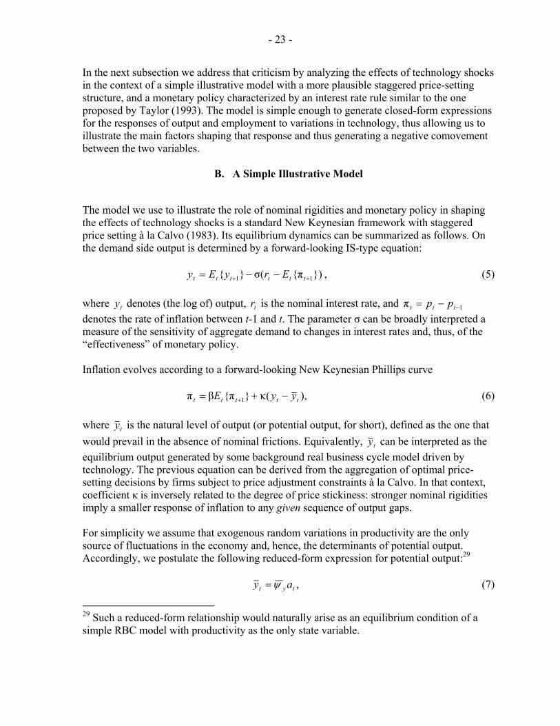
The model we use to illustrate the role of nominal rigidities and monetary policy in shaping the effects of technology shocks is a standard New Keynesian framework with staggered price setting à la Calvo (1983). Its equilibrium dynamics can be summarized as follows. On the demand side output is determined by a forward-looking IS-type equation:

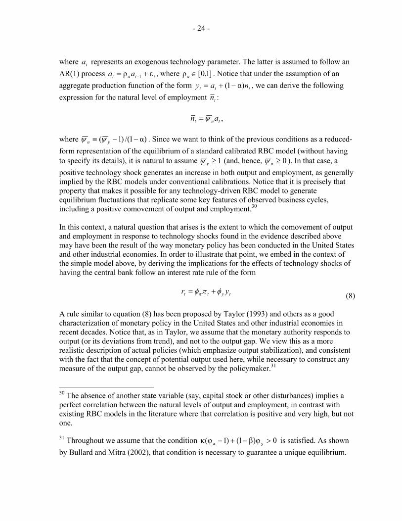
})π{(σ}{ 11 ++ −−= tttttt EryEy , (5) where ty denotes (the log of) output, tr is the nominal interest rate, and 1π −−= ttt pp denotes the rate of inflation between t-1 and t. The parameter σ can be broadly interpreted a measure of the sensitivity of aggregate demand to changes in interest rates and, thus, of the “effectiveness” of monetary policy. Inflation evolves according to a forward-looking New Keynesian Phillips curve

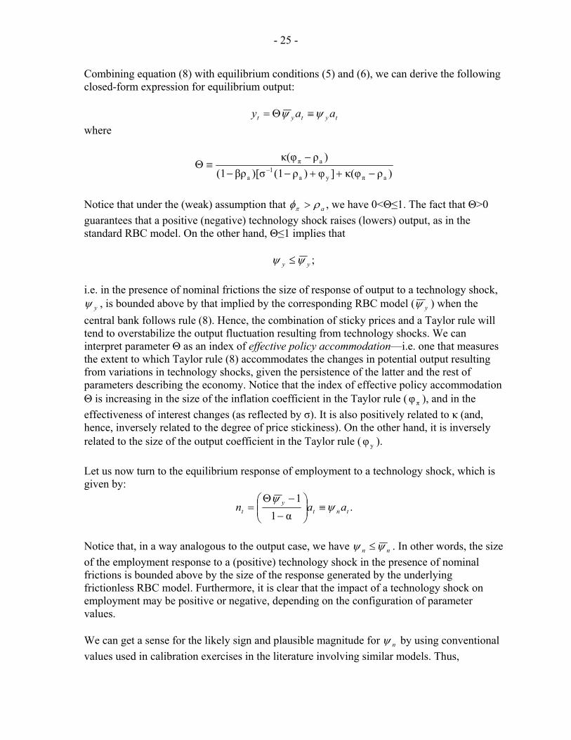
),(κ}π{βπ 1 ttttt yyE −+= + (6) where ty is the natural level of output (or potential output, for short), defined as the one that would prevail in the absence of nominal frictions. Equivalently, ty can be interpreted as the equilibrium output generated by some background real business cycle model driven by technology. The previous equation can be derived from the aggregation of optimal price-setting decisions by firms subject to price adjustment constraints à la Calvo. In that context, coefficient κ is inversely related to the degree of price stickiness: stronger nominal rigidities imply a smaller response of inflation to any given sequence of output gaps. For simplicity we assume that exogenous random variations in productivity are the only source of fluctuations in the economy and, hence, the determinants of potential output. Accordingly, we postulate the following reduced-form expression for potential output:29

,tyt ay ψ= (7)

29 Such a reduced-form relationship would naturally arise as an equilibrium condition of a simple RBC model with productivity as the only state variable.

- 24 -

where ta represents an exogenous technology parameter. The latter is assumed to follow an AR(1) process ttat aa ερ 1 += − , where ]1,0[ρ ∈a . Notice that under the assumption of an aggregate production function of the form ttt nay )α1( −+= , we can derive the following expression for the natural level of employment tn :

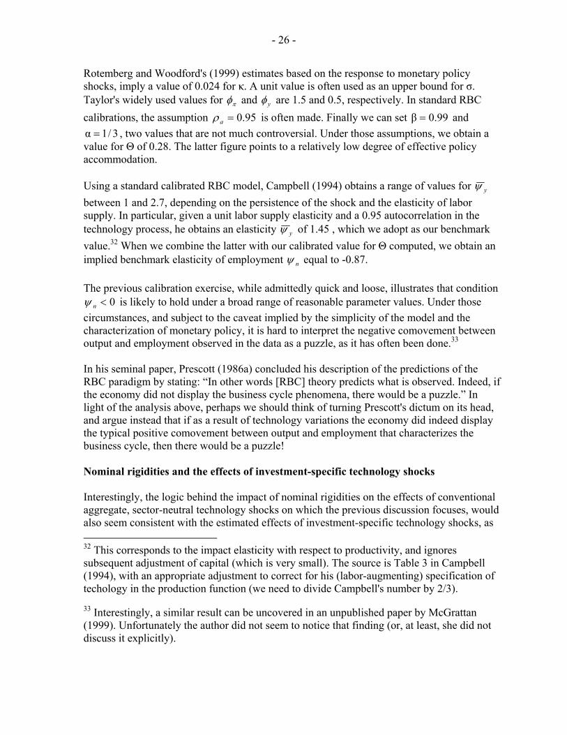
,tnt an ψ= where )α1/()1( −−≡ yn ψψ . Since we want to think of the previous conditions as a reduced-form representation of the equilibrium of a standard calibrated RBC model (without having to specify its details), it is natural to assume 1≥yψ (and, hence, 0≥nψ ). In that case, a positive technology shock generates an increase in both output and employment, as generally implied by the RBC models under conventional calibrations. Notice that it is precisely that property that makes it possible for any technology-driven RBC model to generate equilibrium fluctuations that replicate some key features of observed business cycles, including a positive comovement of output and employment.30 In this context, a natural question that arises is the extent to which the comovement of output and employment in response to technology shocks found in the evidence described above may have been the result of the way monetary policy has been conducted in the United States and other industrial economies. In order to illustrate that point, we embed in the context of the simple model above, by deriving the implications for the effects of technology shocks of having the central bank follow an interest rate rule of the form

tytt yr φπφπ += (8) A rule similar to equation (8) has been proposed by Taylor (1993) and others as a good characterization of monetary policy in the United States and other industrial economies in recent decades. Notice that, as in Taylor, we assume that the monetary authority responds to output (or its deviations from trend), and not to the output gap. We view this as a more realistic description of actual policies (which emphasize output stabilization), and consistent with the fact that the concept of potential output used here, while necessary to construct any measure of the output gap, cannot be observed by the policymaker.31

30 The absence of another state variable (say, capital stock or other disturbances) implies a perfect correlation between the natural levels of output and employment, in contrast with existing RBC models in the literature where that correlation is positive and very high, but not one.

31 Throughout we assume that the condition 0φ)β1()1φ(κ yπ >−+− is satisfied. As shown by Bullard and Mitra (2002), that condition is necessary to guarantee a unique equilibrium.

- 25 -

Combining equation (8) with equilibrium conditions (5) and (6), we can derive the following closed-form expression for equilibrium output:

tytyt aay ψψ ≡Θ= where

)ρκ(φ]φ)ρ(1)[σβρ(1)ρκ(φ

aπya1

a

aπ

−++−−−

≡Θ −

Notice that under the (weak) assumption that aρφπ > , we have 0<Θ≤1. The fact that Θ>0 guarantees that a positive (negative) technology shock raises (lowers) output, as in the standard RBC model. On the other hand, Θ≤1 implies that

;yy ψψ ≤ i.e. in the presence of nominal frictions the size of response of output to a technology shock,

yψ , is bounded above by that implied by the corresponding RBC model ( yψ ) when the central bank follows rule (8). Hence, the combination of sticky prices and a Taylor rule will tend to overstabilize the output fluctuation resulting from technology shocks. We can interpret parameter Θ as an index of effective policy accommodation—i.e. one that measures the extent to which Taylor rule (8) accommodates the changes in potential output resulting from variations in technology shocks, given the persistence of the latter and the rest of parameters describing the economy. Notice that the index of effective policy accommodation Θ is increasing in the size of the inflation coefficient in the Taylor rule ( πφ ), and in the effectiveness of interest changes (as reflected by σ). It is also positively related to κ (and, hence, inversely related to the degree of price stickiness). On the other hand, it is inversely related to the size of the output coefficient in the Taylor rule ( yφ ). Let us now turn to the equilibrium response of employment to a technology shock, which is given by:

.α1

1tnt

yt aan ψ

ψ≡⎟⎟

⎠

⎞⎜⎜⎝

⎛−

−Θ=

Notice that, in a way analogous to the output case, we have nn ψψ ≤ . In other words, the size of the employment response to a (positive) technology shock in the presence of nominal frictions is bounded above by the size of the response generated by the underlying frictionless RBC model. Furthermore, it is clear that the impact of a technology shock on employment may be positive or negative, depending on the configuration of parameter values. We can get a sense for the likely sign and plausible magnitude for nψ by using conventional values used in calibration exercises in the literature involving similar models. Thus,

- 26 -

Rotemberg and Woodford's (1999) estimates based on the response to monetary policy shocks, imply a value of 0.024 for κ. A unit value is often used as an upper bound for σ. Taylor's widely used values for πφ and yφ are 1.5 and 0.5, respectively. In standard RBC calibrations, the assumption 95.0=aρ is often made. Finally we can set 99.0β = and

3/1α = , two values that are not much controversial. Under those assumptions, we obtain a value for Θ of 0.28. The latter figure points to a relatively low degree of effective policy accommodation. Using a standard calibrated RBC model, Campbell (1994) obtains a range of values for yψ between 1 and 2.7, depending on the persistence of the shock and the elasticity of labor supply. In particular, given a unit labor supply elasticity and a 0.95 autocorrelation in the technology process, he obtains an elasticity yψ of 1.45 , which we adopt as our benchmark value.32 When we combine the latter with our calibrated value for Θ computed, we obtain an implied benchmark elasticity of employment nψ equal to -0.87. The previous calibration exercise, while admittedly quick and loose, illustrates that condition

0<nψ is likely to hold under a broad range of reasonable parameter values. Under those circumstances, and subject to the caveat implied by the simplicity of the model and the characterization of monetary policy, it is hard to interpret the negative comovement between output and employment observed in the data as a puzzle, as it has often been done.33 In his seminal paper, Prescott (1986a) concluded his description of the predictions of the RBC paradigm by stating: “In other words [RBC] theory predicts what is observed. Indeed, if the economy did not display the business cycle phenomena, there would be a puzzle.” In light of the analysis above, perhaps we should think of turning Prescott's dictum on its head, and argue instead that if as a result of technology variations the economy did indeed display the typical positive comovement between output and employment that characterizes the business cycle, then there would be a puzzle! Nominal rigidities and the effects of investment-specific technology shocks Interestingly, the logic behind the impact of nominal rigidities on the effects of conventional aggregate, sector-neutral technology shocks on which the previous discussion focuses, would also seem consistent with the estimated effects of investment-specific technology shocks, as 32 This corresponds to the impact elasticity with respect to productivity, and ignores subsequent adjustment of capital (which is very small). The source is Table 3 in Campbell (1994), with an appropriate adjustment to correct for his (labor-augmenting) specification of techology in the production function (we need to divide Campbell's number by 2/3).

33 Interestingly, a similar result can be uncovered in an unpublished paper by McGrattan (1999). Unfortunately the author did not seem to notice that finding (or, at least, she did not discuss it explicitly).

- 27 -

reported in Fisher (2003) and further discussed in Section III above. The argument can be made most clearly in the context of a sticky price version of a model like that in GHK (2000). Once again, let us for simplicity assume that the relationship ttt pmy −= holds in equilibrium, and that both tm and tp are pre-determined relative to the shock. In that case firms will want to produce the same quantity of the good but, in contrast with the case of neutral technology shocks, in order to do so they will need to employ the same level of inputs, since the efficiency of the latter has not been affected (only newly purchased capital goods will enhance that productivity in the future). That property of I-shocks is illustrated in Smets and Wouters (2003a) in the context of a much richer DSGE model. In particular, those authors show that even in the presence of the substantial price and wage rigidities estimated for the U.S. economy, a positive I-shock causes output and labor input to increase simultaneously, in a way consistent with the Fisher (2003) VAR evidence. In fact, as shown in Smets and Wouters (2003a), the qualitative pattern of the joint response of output and hours to an I-shock is not affected much when they simulate the model with all nominal rigidities turned off. Evidence on the role of nominal rigidities A number of recent papers have provided evidence, often indirect, on the possible role of nominal rigidities as a source of the gap between the estimated responses of output and labor input measures to a technology shock and the corresponding predictions of an RBC model. We briefly describe a sample of those papers next. Models with nominal rigidities imply that the response of the economy to a technology shock (or to any other shock, for that matter) will generally depend on the endogenous response of the monetary authority, and should thus not be invariant to the monetary policy regime in place. Galí, López-Salido, and Vallés (2003; henceforth, GLV) exploit that implication, and try to uncover any differences in the estimated response to an identified technology shock across subsample periods. Building on the literature that points to significant differences in the conduct of monetary policy between the pre-Volcker and the Volcker-Greenspan periods, they estimate a four-variable structural VAR with a long-run restriction as in Galí (1999) for each of those subsample periods. Their evidence points to significant differences in the estimated responses to a technology shock. In particular, they show that the decline in hours in response to a positive technology shock is much more pronounced in the pre-Volcker period, being hardly significant in the Volcker-Greenspan. That evidence is consistent with the idea that monetary policy in the latter period has focused more on the stabilization of inflation, and not so much on the stabilization of economic activity.34

34 The analysis in GLV (2003) has been extended by Francis, Owyang, and Theodorou (2004) to other G-7 countries. They uncover substantial differences across countries in the joint response of employment, prices and interest rates to technology shocks, and argue that some of those differences can be grounded in differences in the underlying interest rate rules.

- 28 -

Some evidence at the micro-level is provided by Marchetti and Nucci (2004), who exploit a detailed data set containing information on output, inputs, and price-setting practices for a large panel of Italian manufacturing firms. Using a modified Solow residual approach they construct a time series for TFP at the firm level, and estimate the responses of a number of firm-specific variables to an innovation in the corresponding technology measure. Among other findings, they provide evidence of a negative impact effect of a technology shock on labor input. Most interesting, Marchetti and Nucci (2004) also exploit firm-specific information regarding the frequency of price adjustments. They split the sample of firms according to the frequency of their price revisions: “flexible” price firms (adjust prices every three months or more often) and "sticky" price firms (adjusting every six months or less often). They find that the negative response of employment to a positive technology shock is larger (and significant) in the case of “sticky” price firms, and much weaker (and statistically insignificant) for “flexible” price firms. That evidence suggests that nominal rigidities may be one of the factors underlying the estimated effects of technology shocks.35 Real explanations Several authors have proposed explanations for the evidence described in Section II that do not rely on the presence of nominal rigidities. Such "real" explanations generally involve some modification of the standard RBC model. Next we briefly describe some of those explanations. Francis and Ramey (2003a) propose two modifications of an otherwise standard RBC model that can potentially account for the negative comovement of output and hours in response to a technology shock. The first model incorporates habit formation in consumption and capital adjustment costs. As shown in Francis and Ramey (2003a), a calibrated version of that model can account for many of the estimated effects of technology shocks. In particular, the response to a permanent improvement in technology of consumption, investment and output is more sluggish than in the standard model with no habits or capital adjustment costs. If that dampening effect is sufficiently strong, the increase in output may be smaller than the increase in productivity itself, thus causing a reduction in hours. The latter decline is consistent with the optimal decision of households to consume more leisure (despite the higher wage) as a consequence of a dominant income effect.36 A similar mechanism underlies the modification of the basic RBC model proposed by Wen (2001), who assumes a utility function with a subsistence level of consumption (equivalent to a constant habit).

35 A less favorable assessment is found in Chang and Hong (2003), who conduct a similar exercise using four-digit U.S. manufacturing industries. Relying on evidence of sectoral nominal rigidities based on the work of Bils and Klenow (2002), they find weak evidence of contractionary effects and correlation with measures of price stickiness.

36 See Lettau and Uhlig (2000) for a detailed analysis of the properties of an RBC model with habit formation. As pointed out by Francis and Ramey, Lettau and Uhlig seem to dismiss the assumption of habits on the grounds that it yields “counterfactual cyclical behavior.”

- 29 -

The second modification of the RBC model proposed by Francis and Ramey (2003a) hinges on the assumption of no substitutability between labor and capital in production. In that context the only way to increase output in the short run is by increasing the workweek of capital. Furthermore, hours beyond the standard workweek generate additional disutility. In such a model a permanent increase in labor-augmenting technology is shown to generate a short-run decline in hours. The intuition is simple, and in the final analysis not much different from other modifications proposed. While output increases in the short run (due to increased investment opportunities), that increase is not sufficient to compensate for the fact that any quantity of output can now be produced with less employment (per shift) and a shorter workweek. Rotemberg (2003) develops a version of the RBC model in which technological change diffuses much more slowly than implied by conventional specifications found in the RBC literature. The rate at which technology is adopted is calibrated on the basis of the micro studies on speed of diffusion. Rotemberg shows that when the smooth technology process is embedded in the RBC model it generates small short-run fluctuations in output and employment, which are largely unrelated to the cyclical variations associated with detrended measured of employment and output. In particular, a positive innovation to technology that diffuses very slowly generates a very large wealth effect (relative to the size of the innovation), which in turn leads households to increase their consumption of leisure. As a result, both hours and output experience a short run decline in response to a technology shock of a typical size, before they gradually increase above their initial levels. Because those responses are so smooth, they imply very small movements at cyclical frequencies. It follows that technology shocks with such characteristics will only account for a small fraction of observed cyclical fluctuations in output and hours. Collard and Dellas (2002) emphasize an additional mechanism, specific to an open economy, through which technology shocks may induce short-run negative comovements between output and labor input even in the absence of nominal rigidities. They analyze a two-country RBC model with imperfect substitutability between domestic and foreign consumption goods. If that substitutability is sufficiently low, a positive technology shock in the home country triggers a large deterioration in its terms of trade (i.e., a large decline in the price of domestic goods relative to foreign goods). That change in relative prices may induce households to increase their consumption of leisure at any given product wage, thus contracting labor supply and lowering hours. The quantitative analysis of a calibrated version of their model suggests that while technology shocks may be a non-negligible source of output fluctuations, their role is likely to be very small as a driving force behind hours fluctuations. The papers discussed in this section provide examples of model economies that can account for the evidence regarding the effects of technology shocks without relying on any nominal frictions. On the basis of that evidence it is not possible to sort out the relative role played by "nominal" and "real" frictions in accounting for the evidence. The reason is simple: there is no clear mapping between the estimated coefficients in a structural VAR and the underlying structural parameters that determine the degree of those frictions. As a result, estimated VARs cannot serve as the basis of the sort of counterfactual simulations that would allow us

- 30 -

to uncover the implied effects of technology shocks if either “nominal” or “real” frictions were not present. Such counterfactual exercises require the use of an estimated structural model. In the next section we turn our attention to one such model.

V. TECHNOLOGY SHOCKS AND THE BUSINESS CYCLE IN AN ESTIMATED DSGE MODEL

In this section we try to sort out the merits of the two types of explanations discussed above by estimating and analyzing a framework that incorporates both types of frictions, and that is sufficiently rich to be taken to the data. The features that we incorporate include habit formation in consumption, staggered price and wage-setting à la Calvo, flexible indexation of wages and prices to lagged inflation, and a monetary policy rule of the Taylor type with interest rate smoothing. Several examples of estimated general equilibrium models can be found in the literature. Our framework is most closely related to the one used in Rabanal (2003), with two main differences. First, we allow for a unit root in the technology process in a way consistent with the assumptions underlying the identification strategy pursued in Section II. Second, we ignore the cost channel mechanism allowed for in Rabanal (2003), in light of the evidence in that paper suggesting an insignificant role for that mechanism. We estimate the parameters of the model using Bayesian methods, and focus our analysis on the implications of the estimated model regarding the effects of technology shocks and the contribution of the latter to the business cycle. The use of a structural estimated model allows us to determine, by means of counterfactual simulations, the role played by different factors in accounting for the estimated effects of technology shocks. Last but not least, the estimated model gives us an indication of the nature of the shocks that have played a dominant role as a source of postwar business cycles. The use of Bayesian methods to estimate DSGE models has increased over recent years, in a variety of contexts.37 Fernández-Villaverde and Rubio-Ramírez (2004) show that parameter estimation is consistent in the Bayesian framework even under model misspecification. Smets and Wouters (2003a, 2003b) estimate a model with capital accumulation, and both nominal and real rigidities for the euro area and the United States. Lubik and Schorfheide (2004) use the Bayesian framework to estimate a small-scale model allowing for indeterminacy. Rabanal (2003) estimates a general equilibrium model for the United States and the euro area in search for cost channel effects of monetary policy.38 37 However, the existing literature on estimating general equiilibrium models using Bayesian methods assumes that all shocks are stationary, even when highly correlated. A novelty of this paper is that we introduce a permanent technology shock. Ireland (2004) estimates a general equilibrium model with permanent technology shocks, using maximum likelihood.

38 A somewhat different estimation strategy is the one followed by Christiano, Eichenbaum, and Evans (2003), Altig and others (2003), and Boivin and Giannoni (2003), who estimate general equilibrium models by matching model's implied impulse-response functions to the estimated ones.

- 31 -

Next we summarize the set of equilibrium conditions of the model.39 The demand side of the model is represented by the Euler-like equation

,)1)(ρ1(})π{)(1( 11 tgtttttt gbErbyEyb −−+−−−∆=∆ ++ (9) which modifies equation (5) above by allowing for some external habit formation (indexed by parameter b), and introducing a preference shock }{ tg that follows an AR(1) process with coefficient gρ . Underlying equation (9) is the assumption that preferences are separable between consumption and hours, and logarithmic in the quasidifference of consumption in order to preserve the balanced growth path property.40 Aggregate output and hours are related by the simple log-linear production function

.ttt nay += Equivalently, and using a tilde to denote variables normalized by current productivity (in order to induce stationarity), we have

.~tt ny =

Log-linearization of the optimal price-setting condition around the zero-inflation steady state yields an equation describing the dynamics of inflation as a function of the deviations of the average (log) markup from its steady-state-level, which we denote by p

tµ :41

),µκπγπγπ 11 tptpttftbt u(}{E −−+= +− (11)

where )/( ppb βη1ηγ += , )βηβ/(1γ pf += , )]()/[)(( ppppp βη1θθ1βθ1κ +−−= , pθ is the probability of not adjusting prices in any given period, and ]1,0[η ∈p is the degree of price

indexation to lagged inflation. Notice that ttttpt APW ω~)]/(log[µ −≡−= is the price markup,

where ttt a−= ωω~ is the real wage per efficiency unit. Variable tu denotes exogenous variations in the desired price markup. 39 Details can be found in an appendix available from the authors upon request.

40 Specifically, every household maximizes the following utility function:

∑∞

=

+

− +−−

0

1

1 ]1

)()log([

t

jtj

tj

ttt

oN

bCCGEϕ

βϕ

,

subject to a usual budget constraint. The preference shock evolves, expressed in logarithms, as g

ttggt gGg ερ)ρ1( 1 ++−= − . 41 See Smets and Wouters (2003a) for a derivation of the price- and wage-setting equations.

- 32 -

Log-linearization of the optimal wage-setting condition yields the following equation for the dynamics of the (normalized) real wage:

),µ(β1

κ}π{

β1βπ

β1)βη1(

πβ1

η}{

β1β

β11}ω~{

β1βω~

β11ω~

1

1111

twt

wttt

w

tw

ttttttt

vE

aEaE

−+

−+

++

+−

++∆

++∆

+−

++

+=

+

−++−

(12)

where wθ denotes the fraction of workers that do not re-optimize their wage, ]1,0[η ∈w is the degree of wage indexation to lagged inflation, and )]ε1(θ/[)θ1)(βθ1(κ wwwww ϕ+−−= , where wε is the wage elasticity of labor demand in the steady state. Also notice that

)1

~1

~1

1(ω~µ 1 ttttttwt na

bbgy

bby

bϕ+∆

−+−

−−

−−≡ − is the wage markup. Variable vt denotes

exogenous variations in the desired wage markup. Finally, we close the model by assuming that the monetary authority adjusts interest rates in response to changes in inflation and output growth according to the rule:

,))1()1( t1 ttyrrtrt zyrr +∆−+−+= − φφπφφφ π (13) where zt is an exogenous monetary shock.42 The exogenous driving variables are assumed to evolve as follows:

.1

1

1

1

ztt

vttvt

uttut

gttgt

attt

z

vv

uu

gg

aa

ε

ερ

ερ

ερ

ε

=

+=

+=

+=

+=

−

−

−

−

Notice that while we do not observe tω

~ and ty~ , the two variables are related as follows:

,~~tttt yy −=− ωω

42 Following Erceg and Levin (2003), we assume that the Federal Reserve reacts to output growth rather than to the output gap. An advantage of following such a rule, as Orphanides and Williams (2002) stress, is that mismeasurement of the level of potential output does not affect the conduct of monetary policy (as opposed to using some measure of detrended output to estimate the output gap).

- 33 -

and tt y−ω is an observable variable, which should be stationary in equilibrium. In the next section, we explain how to write the likelihood function in terms of the five observable variables: output growth, inflation, the nominal interest rate, hours, and the real wage-output ratio.

A. Parameter Estimation

Data We estimate the model laid out in the previous section using U.S. quarterly time series for five variables: real output, inflation, real wages, hours, and interest rates. The sample period is 1948:1 to 2002:4. For consistence with the analysis in Section II, we use the same series for output and hours. Our measure of nominal wages is the compensation per hour in the nonfarm business sector (LXNFC), and the measure for the price level is the nonfarm business sector deflator (LXNFI). Finally, we use the quarterly average daily readings of the three-month Treasury bill (FTB3) as the relevant nominal interest rate. To render the series stationary, we detrend hours and the real wage-output ratio using a quadratic trend. We treat inflation, output growth and the nominal interest rate as stationary, and express them in deviations from their sample mean. As is well known from Bayes' rule, the posterior distribution of the parameters is proportional to the product of the prior distribution of the parameters and the likelihood function of the data. Until recently, only well-known and standard distributions could be used. The advent of fast computer processors and Markov Chain Monte Carlo (MCMC) methods has removed this restriction, and a more general class of models and distributions can be used.43 To implement the Bayesian estimation method, we need to be able to evaluate numerically the prior and the likelihood function. Then, we use the Metropolis-Hastings algorithm to obtain random draws from the posterior distribution, from which we obtain the relevant moments of the posterior distribution of the parameters. The likelihood function Let ψ denote the vector of parameters that describe preferences, technology, the monetary policy rule, and the shocks of the model, dt be the vector of endogenous variables (observable or not), zt be the vector of shocks, and εt be the vector of innovations. The system of equilibrium conditions and the process for the exogenous shocks can be written as a second-order difference equation

).ψ()εε( ,ε)ψ(

,)ψ()ψ()ψ()ψ('

1

11

Σ=+=

++=

−

−+

ttttt

ttttt

EzNz

zDdCdBdEA

43 See Fernández-Villaverde and Rubio-Ramírez (2004).

- 34 -

We use standard solution methods for linear models with rational expectations (as in Uhlig, 1999) to write the law of motion in state-space form and the Kalman filter (as in Hamilton, 1994) to evaluate the likelihood of the five observable variables { }',,ω,π, ttttttt ynyrx ∆−= . We denote by )ψ|}({ 1

TttxL = the likelihood function of T

ttx 1}{ = . Priors In this section, we denote by Π(ψ) the prior distribution of the parameters. We present the list of the structural parameters and its associated prior distributions in the first three columns of Table 4. Most of the priors involve uniform distributions for the parameters, which simply restrict the support. We use uniform distributions for the parameter that explains habit formation, for the probabilities of the Calvo lotteries, and for the indexation parameters. The prior for all these parameters has support between 0 and 1, except the probabilities of the Calvo lottery, which are allowed to take values up to 0.9—i.e., we are ruling out average price and wage durations of more than 10 quarters. We try to supplement as much prior information as possible for the model's exogenous shocks. The AR(1) coefficients have uniform prior distributions between 0 and 0.97. Gamma distributions for the standard deviations of the shocks are assumed, to guarantee non-negativity. We select their hyper parameters to match available information for the prior mean standard deviation of the innovations, while allowing reasonable uncertainty in these parameters. For instance, for the monetary policy rule we choose the means of the inflation and output growth coefficients to match the ones proposed by Taylor.44 For the monetary policy shock, we use the standard deviation that comes from running an OLS regression for the Taylor rule equation. In addition, we fix some parameters. The discount factor, we set at β=0.99. The elasticities of product and labor demand are set to 6 (which implying steady state markups of 20 percent). These values are fairly conventional in the literature. Drawing from the posterior From Bayes rule, we obtain the posterior distribution of the parameters as follows:

).ψ()ψ|}({)}{|ψ( 11 Π∝ ==Ttt

Ttt xLxp

The posterior density function is proportional to the product of the likelihood function and the prior joint density function of ψ. Given our priors and the likelihood functions implied by the state-space solution to the model, we are not able to obtain a closed-form solution for the 44 If a random draw of the parameters is such that the model does not deliver a unique and stable solution, we assign a zero likelihood value, which implies that the posterior density will be zero as well. See Lubik and Schorfheide (2003) for an estimated DSGE model allowing for indeterminacy.

- 35 -

posterior distributions. However, we are able to evaluate both expressions numerically. We follow Fernández-Villaverde and Rubio-Ramírez (2004) and Lubik and Schorfheide (2004) and use the random walk Metropolis-Hastings algorithm, to obtain a random draw of size 500,000 from ).}{|ψ( 1

Tttxp = We use the draw to estimate the moments of the posterior

distribution, and to obtain impulse responses and second moments of the endogenous variables.

B. Main Findings

Parameter estimates and second moments The last two columns of Table 4 report the mean and standard deviation of the posterior distributions for all the parameters. Notice that the habit formation parameter is estimated to be 0.42, a value somewhat smaller than that suggested by Christiano, Eichenbaum, and Evans (2003) or Smets and Wouters (2003b). The parameter that measures the elasticity of the marginal disutility of hours, φ, is estimated to be 0.80, which is close to values usually obtained or calibrated in the literature. The average duration of price contracts implied by the point estimate of the price stickiness parameter lies slightly above two quarters. We view this estimate as a “moderate” amount of price stickiness in the economy. Perhaps most surprising is the low degree of wage stickiness uncovered by our estimation method. Such an implausible low estimate may suggest that the Calvo model is not the best formalism to characterize wage dynamics.45 The price indexation coefficient is estimated at a low value, 0.04, suggesting that the pure forward-looking model is a good approximation to inflation dynamics, once we allow for autoregressive price markup shocks. On the other hand, indexation in wage setting is more important, with a posterior mean of 0.42. The coefficients of the interest rate rule suggest a high degree of interest rate smoothing, 0.69, a small response of the interest rate to output growth fluctuations, and a coefficient of the response of the interest rate to inflation of 1.33, which corresponds to a "lean against the wind" monetary policy. The estimated processes for the shocks of the model suggest that all of them are highly auto correlated, with parameters between 0.95 for the price markup shock to 0.91 for the wage markup shock.46

45 Rabanal (2003) finds a similar result for an estimated DSGE model that is only slightly different from the one used here.

46 We have also conducted some subsample stability analysis, splitting the sample into pre-Volcker years and the Volcker-Greenspan era. While there were some small differences in estimated parameters across samples, none of the main conclusions of this section were affected.

- 36 -

Table 5 displays some selected posterior second moments implied by the model estimates and compares them to the data.47 The first two columns present the standard deviation of the observed variables, and their counterparts implied by the estimated model. We can see that the model does a very good job in replicating the standard deviations of output, inflation, and the nominal interest rate. The model also does well in mimicking the unconditional correlation between the growth rates of hours and output: in the data it is 0.75, and in the model it is 0.72. However, it overestimates the standard deviation of hours (3.11 percent in the data and 4.6 percent in the model) and to a lesser extent the real wage-to-output ratio (3.69 percent in the data, 4.44 percent in the model) The effects of technology shocks Next we turn our attention to the estimated model's predictions regarding the effects of technology shocks.48 Figure 7 displays the posterior impulse responses to a permanent technology shock of size normalized to one standard deviation.49 We can observe that the model replicates the VAR-based evidence fairly well, in spite of the differences in the approach. In particular the estimated model implies a persistent decline in hours in response to a positive technology shock, and a gradual adjustment of output to a permanently higher plateau. It takes about four quarters for output to reach its new steady-state level. Hours drop on impact by about 0.4 percentage points and converge monotonically to their initial level afterward.50 The third column of Table 5 reports the second moments of the observed variables conditional on technology shocks being the only driving force. The fourth column shows the fraction of the variance of each variable accounted for by the technology shock.51 We can see that technology shocks do not play a major role in explaining the variability of the five observed variables. They explain 22 percent of the variability of output growth, and 6 percent

47 These second moments were obtained using a sample of 10,000 draws from the 500,000 that were previously obtained with the Metropolis-Hastings algorithm.

48 A related analysis has been carried out independently by Smets and Wouters (2003b), albeit in the context of a slightly different DSGE model.

49 The posterior mean and standard deviations are based on the same sample that was used to obtain the second moments.

50 A similar pattern of responses of output and hours to a technology shock can be found in Smets and Wouters (2003b).

51 We use the method of Ingram, Kocherlakota, and Savin (1994) to recover the structural shocks. This method is a particular case of using the Kalman filter to recover the structural shocks. We assume that the economy is at its steady-state value in the first observation, rather than assuming a diffuse prior. By construction, the full set of shocks replicate perfectly the features of the model.

- 37 -

of the variability of inflation. For the rest of variables, including hours, they explain an insignificant amount of overall volatility. A key result emerges when we simulate the model with technology shocks only: we obtain a correlation between ),( tt ny ∆∆ of -0.49, which contrasts with the high positive correlation between the same variables observed in the data. The last three rows of Table 5 report statistics based on band-pass filtered data. In this case, the series of output growth and hours generated by the estimated model (when all shocks other than technology are turned off) are used to obtain the (log of) levels of hours and output, on which the band-pass filter is applied. Once again we find that technology shocks can only account for a small fraction of the variance of the business cycle component of output and hours. The conditional correlation between those two variables falls to -0.14, from a value of 0.88 for the actual filtered series. The previous findings are illustrated graphically in Figure 7, which displays the business cycle components of log output and log hours associated with technology shocks, according to our estimated model. It is apparent that technology shocks explain only a minor fraction of output fluctuations. This is even more dramatic when we look at fluctuations in hours, in a way consistent with most of the VAR findings. Similar qualitative findings are found in Altig and others (2003), Ireland (2003), and Smets and Wouters (2003b), using slightly different models and/or estimation methods. What are the main sources of economic fluctuations? Which shocks play a more important role in explaining fluctuations in our observed variables? In Table 6 we report the contribution of each shock to the total variance of each variable implied by our model estimates. The shock that explains most of the variance of all variables in our framework is the preference shock, which we can interpret more broadly as a (real) demand shock. It explains above 70 percent of the variance of hours, the real wage-output ratio, and the nominal interest rate. The preference shock also explains 57 percent of the variance of output, and 36 percent of the variance of inflation. On the other hand, the monetary shock only explains approximately 5 percent of output growth and the nominal interest rate, and is an important determinant of inflation variability, contributing to 27 percent of total volatility. Price and wage markup shocks both have some importance in explaining the volatility of all variables, with contributions to the variance that range from 7 percent to 17 percent. Overall, the picture that emerges from Table 6 is that preference shocks are key to explain the volatility of all variables. The monetary and technology shocks have some importance in the sense that they explain about 20 percent of the variance in one of the variables (output growth in the case of technology, inflation in the case of monetary shocks), but their contribution to the remaining variables is very small. The price and wage markup shocks explain a small fraction of variability in all variables. Structural explanations for the estimated effects of technology shocks Finally, we examine which features of the model are driving the negative comovement between hours and output in response to technology shocks. In Table 7 we present the correlation between the business cycle components of output and hours that arises under

- 38 -

several counterfactual scenarios. For each scenario we shut down some of the rigidities of the model and simulate it again while keeping the same value for the remaining parameter estimates. Three features of the model stand out as natural candidates to explain the negative correlation between output and hours: sticky prices, sticky wages, and habit formation. When we shut down each of those we find that the remaining rigidities still induce a large and negative conditional correlation. For instance, in the second row we can see that assuming flexible wages (θw=ηw=0) delivers basically the same correlations. This result is not surprising since nominal wage rigidities do not appear to be important given the parameter estimates. When we assume flexible prices but keep sticky wages and habit formation, things do not change much either. A particular scenario would seem to be of special interest: one with flexible prices and wages, and habit formation. In that case, once again, a similar pattern of correlations emerges. A similar result is obtained by Smets and Wouters (2003b), who interpret it as evidence favorable to some of the real explanations found in the literature. Yet, when we turn off habit formation in our estimated model but keep nominal rigidities operative, we find a qualitatively similar result: the conditional and unconditional correlations between hours and output have the same pattern of signs as that observed in the data. It is only when we shut down all rigidities (nominal and real) that we obtain a positive correlation between hours and output, both conditionally and unconditionally, and in a way consistent with the predictions of the basic RBC model. Finally, we consider a calibration in which the central bank responds exclusively to inflation changes, but not to output. Some authors have argued that the negative comovement of output and hours may be a consequence of an attempt by the monetary authority to overstabilize output. Our results suggest that this cannot be an overriding factor: when we set the coefficient on output growth equal to zero (but keeping both habit formation and nominal rigidities operative) we still obtain a negative conditional correlation between hours and output. In light of the previous findings we conclude that both real rigidities (habit formation, in our model) and nominal rigidities (mostly sticky prices) appear to be relevant factors in accounting for the evidence on the effects of technology shocks. Interestingly, and by way of contrast, both nominal and real rigidities seem to be required in order to account for the empirical effects of monetary policy shocks (see, e.g., Christiano, Eichenbaum, and Evans, 2003) or the dynamics of inflation (e.g., Galí and Gertler, 1999).

VI. CONCLUSIONS

In this paper we have reviewed recent research efforts that seek to identify and estimate the role of technology as a source of economic fluctuations in ways that go beyond the simple unconditional second-moment matching exercises found in the early RBC literature. The number of qualifications and caveats of any empirical exercise that seeks to provide an answer to the above questions is never small. Furthermore, and as is often the case in empirical research in economics, the evidence does not speak with a single voice, even when

- 39 -

similar methods and data sets are used. Those caveats notwithstanding, the bulk of the evidence reported in the paper raises serious doubts about the importance of changes in aggregate technology as a significant (or, even more, a dominant) force behind business cycles, in contrast with the original claims of the RBC literature. Instead it points to demand factors as the main force behind the strong positive comovement between output and labor input measures that is the hallmark of the business cycle.

VII. ADDENDUM: A RESPONSE TO ELLEN MCGRATTAN

In her comments to the present paper, Ellen McGrattan (2004) dismisses the evidence on the effects of technology shocks based on structural vector autoregressions (SVARs) that rely on long-run identifying restrictions. The purpose of this addendum is to explain why we think McGrattan's analysis and conclusions are misleading. Since some of her argument and the evidence she provides is based on her recent working paper with Chari and Kehoe, our discussion often refers directly to that paper (Chari, Kehoe, and McGrattan (2004; henceforth, CKM). Our main point is easy to summarize. McGrattan and CKM study a number of model economies, all of which predict that hours should rise in response to a positive technology shock. Yet, when they estimate a SVAR on data generated by those models, the resulting impulse responses show a decline in hours in response to such a shock (with one exception, to be discussed below). McGrattan presents her findings and those in CKM as an illustration of a general flaw with SVARs. But we find that conclusion unwarranted. What McGrattan and CKM really show is that a misidentified and/or misspecified SVAR often leads to incorrect inference. As McGrattan herself acknowledges, in her example of a "standard" RBC model (as well as in all but one of the examples in CKM) the assumptions underlying the data generating model are inconsistent with the identifying assumption in the VAR: technology is stationary, or non-technology shocks have a permanent effect on productivity, or the order of integration of hours is wrong.52 In those cases the finding of incorrect inference is neither surprising nor novel, since it restates points that have already been made in the literature.53 Furthermore, that conclusion should be contrasted with that of Erceg, Guerrieri, and Gust (2004; EGG, henceforth), who show that when the SVAR is correctly specified and the identifying restrictions are satisfied by the underlying data-generating models, the estimated responses to technology shocks match (at least qualitatively) the theoretical ones. 52 In the one case where the VAR is identified correctly, it yields the correct qualitative responses, though with some quantitative bias resulting from the inability to capture the true dynamics with a low-order VAR. This result has been shown in Erceg, Guerrieri, and Gust (2004).

53 See Cooley and Dwyer (1998) and Christiano, Eichenbaum and Vigfusson (2003), among others.

- 40 -

We think that, when properly used, SVARs provide an extremely useful guide for developing business cycle theories. Evidence on the effects of particular shocks that is shown to be robust to a variety of plausible identification schemes should not be ignored when developing and refining DSGE models that will be used for policy analysis. On the one hand, that requirement imposes a stronger discipline on model builders than just matching the patterns of unconditional second moments of some time series of interest, the approach traditionally favored by RBC economists. On the other hand, it allows one to assess the relevance of alternative specifications without knowledge of all the driving forces impinging on the economy.54 Another finding in CKM that may seem striking to many readers is that their business accounting framework produces a rise in hours in response to a positive technology shock, in contrast with the evidence summarized in Section II of our paper. Below, we conjecture that such a result hinges critically on treating the conventional Solow residual as an appropriate measure of technology, in contrast to the wealth of evidence suggesting the presence of significant procyclical error in that measure of technology. By way of contrast, most of the SVAR-based findings on the effects of technology shocks overviewed in the present paper rely on identifying assumptions that are much weaker than those required for the Solow residual to be a suitable measure of technology. Next, we elaborate on the previous points, as well as on other issues raised by McGrattan's comment. First, we try to shed some light on why the estimated SVARs do not recover the model-generated impulse responses. Second, we provide a conjecture about why CKM's estimated model would predict an increase in hours in response to a positive technology shock, even if the opposite were to be true. Finally, we comment on CKM's proposed alternative to SVARs.

A. Why Does the SVAR Evidence Fail to Match the McGrattan and CKM Models' Predictions?

The reason why the SVAR estimates reported by McGrattan fail to recover the joint response of output and hours implied by her RBC model should not be viewed as reflecting an inherent flaw in the SVAR approach. Instead it is most likely a consequence of misspecification and misidentification of the SVAR used. First, and most flagrantly, the “geometric growth” specification of technology assumed in the McGrattan exercise implies that technology shocks will only have temporary effects on labor productivity. A maintained assumption in Galí (1999) and in Section II.A above, is the existence of a unit root in the technology process, underlying the observed unit root in productivity. It is clear that if a researcher holds an inherent belief in the stationarity of technology she will not want to use that empirical approach to estimate the effects of technology shocks. We find the notion that technology shocks don't have permanent effects 54 See Christiano, Eichenbaum, and Vigfusson (2003) for an illustration of the usefulness of that approach.

- 41 -

hard to believe, but we cannot offer any proof (though we have provided suggestive evidence along those lines in Section III.A). In any event, we find it useful to point out that the literature contains several examples, reviewed in Section II, that do not rely on the unit root assumption, and that yield results similar to those in Galí (1999).55 In principle, CKM appear to overcome the previous misidentification problem by using as a data-generating mechanism an RBC model that assumes a “unit root” in technology. They consider two versions of that model (“preferred” and “baseline”), which we discuss in turn. Their "preferred" specification fails to satisfy the identifying restriction of the VAR in another important dimension: because of the endogeneity of technology in their model (reflected in the non-zero off-diagonal terms in the process describing the driving forces), shocks that are non-technological in nature are going to have an effect on the level of technology and, hence, on productivity. As a result, the identification underlying the SVAR will be incorrect and inference will be distorted. The two misidentification problems just discussed should not affect the CKM “baseline” specification, for technology in the latter is assumed to follow an exogenous random walk process. Yet, when we look at the properties of that model we uncover a misspecification problem in the VAR used. In a nutshell, and as it is the case for most RBC models found in the literature, CKM's baseline model implies that hours worked follow a stationary process, though they estimate the SVAR using first-differenced hours. The potential problems associated with that misspecification were originally pointed out by CEV (2003) and have been discussed extensively in Section III of the present paper.56 Interestingly, CKM provide one example (the “exception” we referred to above) in which the estimated SVAR satisfies both the key long-run identifying restriction (technology is exogenous and contains a unit root) and is correctly specified (hours are introduced in levels). In that case, and not surprisingly, the SVAR makes a correct inference: hours are estimated to rise in response to a technology shock, as the model predicts. While CKM acknowledge that fact, they instead focus on the finding that the estimated impulse response shows a non-negligible bias. This is an interesting point, but it is not central to the controversy regarding the effects of technology shocks: the latter has focused all along on the estimated sign of the comovement of output and hours, not on the size of the responses. Nor is it novel: it is one of the two main findings in EGG, who already point out and analyze the role played by the slow adjustment of capital in generating that downward bias. Unfortunately, neither McGrattan nor CKM emphasize EGG's second main finding, which is highly relevant for their purposes: using both a standard RBC model and a New Keynesian 55 See BFK (1999), Francis, Owyang, and Thedorou (2003), and Pesavento and Rossi (2004).

56 CKM's discussion of that problem is somewhat obscured by their reference to “the insufficient number of lags in the VAR,” as opposed to just stating that hours are over-differenced. See also Marcet (2004) for a more general discussion of the consequences (or lack thereof) of overdifferencing.

- 42 -

model with staggered wage and price setting as data-generating mechanisms, they conclude that the estimated responses to a technology shock, using the same SVAR approach as in Galí (1999), look like the true responses to that shock in both models, at least from a qualitative viewpoint (leading to a rise in hours in the former case, and to a drop in the latter, in a way consistent with the models' predictions).

B. Why Does the CKM Accounting Framework Predict a Rise in Hours?

The framework used by McGrattan in Section II.2 of her comment is unlikely to be recognized by most macroeconomists as a “standard RBC model,” the title of the subsection notwithstanding. Instead, it consists of a version of the business cycle accounting framework originally developed in CKM. That framework consists of a standard RBC model with four driving forces (or “wedges,” in their terminology). One of those driving forces, which enters the production function as a conventional productivity parameter, is interpreted as a technology shock. Two other driving forces are broadly interpreted as a labor market and an investment wedge. The fourth is government spending. After assuming functional forms for preferences and technology as well as a conventional calibration of the associated parameters conventional in the RBC literature, CKM estimates a VAR model for the four driving forces using time series for output, hours, investment, and government consumption. Let us put aside some of the issues regarding the suitability of SVARs discussed in the previous section to turn to a different question: Why does the estimated CKM accounting framework predict an increase in hours in response to a positive technology shock? The interest of the question may be puzzling to some readers: after all, the CKM model looks like a standard RBC model augmented with many shocks. But that description is not accurate in a subtle, but important dimension: the disturbances/wedges in the CKM accounting framework are not orthogonal to each other, having instead a rich dynamic structure. Thus, nothing prevents, at least in principle, some of the nontechnology wedges from responding to a technology shock in such a way as to generate a negative comovement between output and hours in response to that shock. After all, the increase in markups following a positive technology shock is precisely the mechanism through which a model with nominal rigidities can generate a decline in hours. Here, we can only speculate on the sources of the sign of the response of hours predicted by the CKM model. But a cursory look at the structure of the model, and the approach to uncovering its shocks, points to a very likely candidate for that finding: the CKM measure of the technology parameter corresponds to the gap between (the log of) GDP and a weighted average of (the log of) capital and (the log of) hours, with the weights based on average income shares. In other words, the CKM measure of technology corresponds for all practical purposes to the conventional Solow (1957) residual. In adopting that approach to identification of technology, CKM are brushing aside two decades of research pointing to the multiple shortcomings of the Solow residual as a measure of short-run variations to technology, from Hall (1988) to BFK (1999). In the absence of any adjustments for market power, variable utilization of inputs, and other considerations, the Solow residual, as an index of technological change, is known to be ridden with a large (and highly procyclical) measurement error.

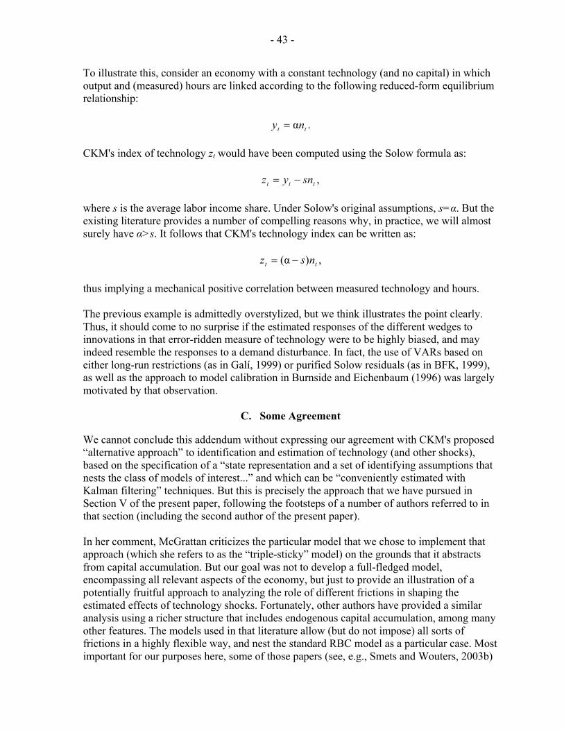
- 43 -

To illustrate this, consider an economy with a constant technology (and no capital) in which output and (measured) hours are linked according to the following reduced-form equilibrium relationship:

.α tt ny = CKM's index of technology zt would have been computed using the Solow formula as:

,ttt snyz −= where s is the average labor income share. Under Solow's original assumptions, s=α. But the existing literature provides a number of compelling reasons why, in practice, we will almost surely have α>s. It follows that CKM's technology index can be written as:

,)α( tt nsz −= thus implying a mechanical positive correlation between measured technology and hours. The previous example is admittedly overstylized, but we think illustrates the point clearly. Thus, it should come to no surprise if the estimated responses of the different wedges to innovations in that error-ridden measure of technology were to be highly biased, and may indeed resemble the responses to a demand disturbance. In fact, the use of VARs based on either long-run restrictions (as in Galí, 1999) or purified Solow residuals (as in BFK, 1999), as well as the approach to model calibration in Burnside and Eichenbaum (1996) was largely motivated by that observation.

C. Some Agreement

We cannot conclude this addendum without expressing our agreement with CKM's proposed “alternative approach” to identification and estimation of technology (and other shocks), based on the specification of a “state representation and a set of identifying assumptions that nests the class of models of interest...” and which can be “conveniently estimated with Kalman filtering” techniques. But this is precisely the approach that we have pursued in Section V of the present paper, following the footsteps of a number of authors referred to in that section (including the second author of the present paper). In her comment, McGrattan criticizes the particular model that we chose to implement that approach (which she refers to as the “triple-sticky” model) on the grounds that it abstracts from capital accumulation. But our goal was not to develop a full-fledged model, encompassing all relevant aspects of the economy, but just to provide an illustration of a potentially fruitful approach to analyzing the role of different frictions in shaping the estimated effects of technology shocks. Fortunately, other authors have provided a similar analysis using a richer structure that includes endogenous capital accumulation, among many other features. The models used in that literature allow (but do not impose) all sorts of frictions in a highly flexible way, and nest the standard RBC model as a particular case. Most important for our purposes here, some of those papers (see, e.g., Smets and Wouters, 2003b)

- 44 -

have analyzed explicitly the effects of technology shocks implied by their estimated models. In a way consistent with our findings above, those effects have been shown to imply a negative response of hours to a positive technology shock. Unfortunately, McGrattan reports no comparable evidence for her “triple-sticky model with investment,” though we conjecture that the latter would imply a similar response.

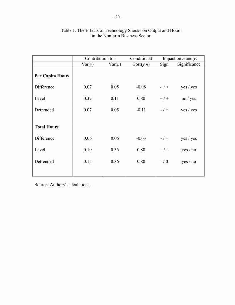
- 45 -

Table 1. The Effects of Technology Shocks on Output and Hours in the Nonfarm Business Sector

Source: Authors’ calculations.

Contribution to: Conditional Impact on n and y: Var(y) Var(n) Corr(y,n) Sign Significance

Per Capita Hours Difference 0.07 0.05 -0.08 - / + yes / yes Level 0.37 0.11 0.80 + / + no / yes Detrended 0.07 0.05 -0.11 - / + yes / yes Total Hours Difference 0.06 0.06 -0.03 - / + yes / yes Level 0.10 0.36 0.80 - / - yes / no Detrended 0.15 0.36 0.80 - / 0 yes / no

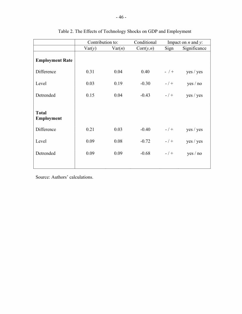
- 46 -

Table 2. The Effects of Technology Shocks on GDP and Employment

Source: Authors’ calculations.

Contribution to: Conditional Impact on n and y: Var(y) Var(n) Corr(y,n) Sign Significance

Employment Rate Difference 0.31 0.04 0.40 - / + yes / yes Level 0.03 0.19 -0.30 - / + yes / no Detrended 0.15 0.04 -0.43 - / + yes / yes Total Employment

Difference 0.21 0.03 -0.40 - / + yes / yes Level 0.09 0.08 -0.72 - / + yes / yes Detrended 0.09 0.09 -0.68 - / + yes / no

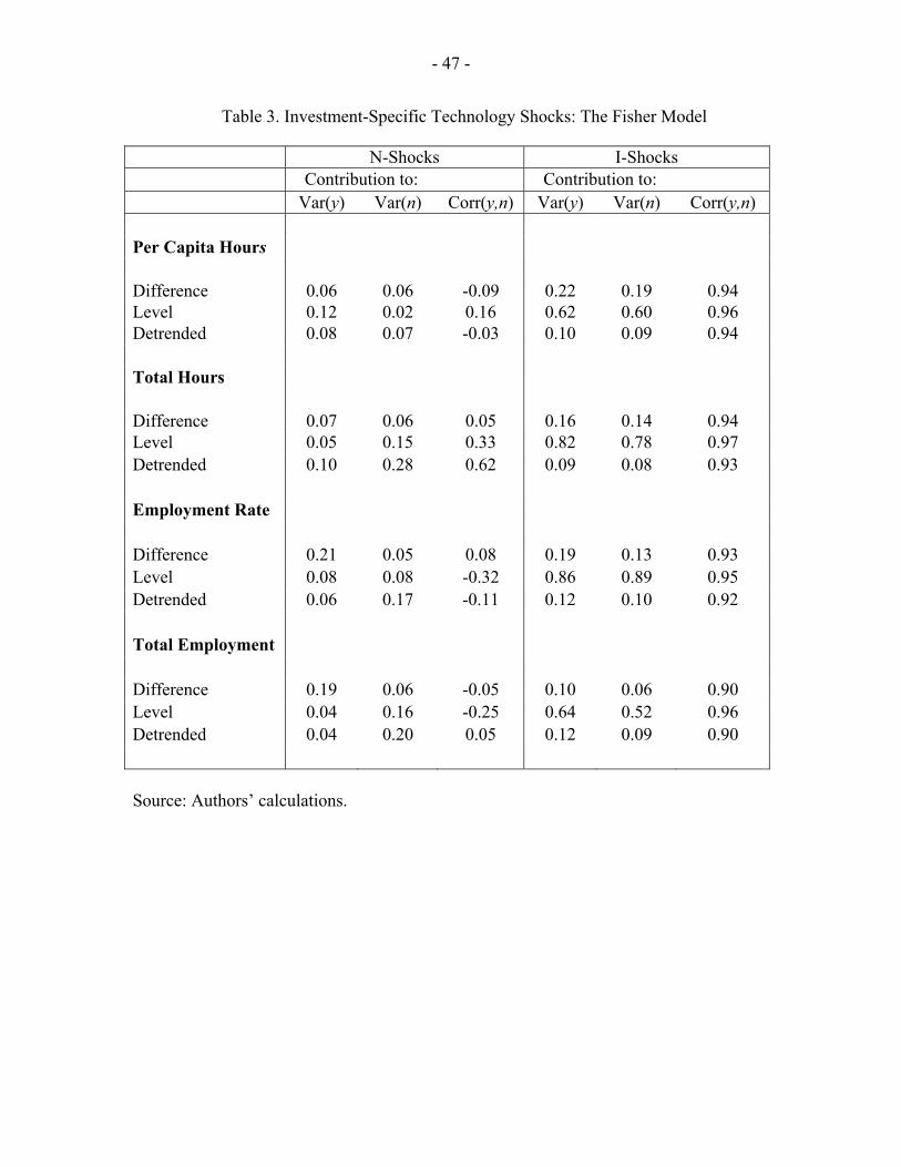
- 47 -

Table 3. Investment-Specific Technology Shocks: The Fisher Model

Source: Authors’ calculations.

N-Shocks I-Shocks Contribution to: Contribution to: Var(y) Var(n) Corr(y,n) Var(y) Var(n) Corr(y,n)

Per Capita Hours Difference 0.06 0.06 -0.09 0.22 0.19 0.94 Level 0.12 0.02 0.16 0.62 0.60 0.96 Detrended 0.08 0.07 -0.03 0.10 0.09 0.94 Total Hours Difference 0.07 0.06 0.05 0.16 0.14 0.94 Level 0.05 0.15 0.33 0.82 0.78 0.97 Detrended 0.10 0.28 0.62 0.09 0.08 0.93 Employment Rate Difference 0.21 0.05 0.08 0.19 0.13 0.93 Level 0.08 0.08 -0.32 0.86 0.89 0.95 Detrended 0.06 0.17 -0.11 0.12 0.10 0.92 Total Employment Difference 0.19 0.06 -0.05 0.10 0.06 0.90 Level 0.04 0.16 -0.25 0.64 0.52 0.96 Detrended 0.04 0.20 0.05 0.12 0.09 0.90

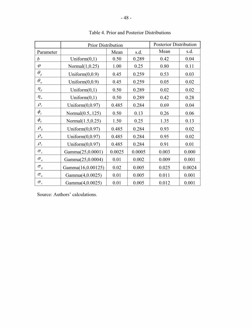
- 48 -

Table 4. Prior and Posterior Distributions

Prior Distribution Posterior Distribution Parameter Mean s.d. Mean s.d. b Uniform(0,1) 0.50 0.289 0.42 0.04 ϕ Normal(1,0.25) 1.00 0.25 0.80 0.11

pθ Uniform(0,0.9) 0.45 0.259 0.53 0.03 wθ Uniform(0,0.9) 0.45 0.259 0.05 0.02 pη Uniform(0,1) 0.50 0.289 0.02 0.02 wη Uniform(0,1) 0.50 0.289 0.42 0.28 rρ Uniform(0,0.97) 0.485 0.284 0.69 0.04 yφ Normal(0.5,.125) 0.50 0.13 0.26 0.06 πφ Normal(1.5,0.25) 1.50 0.25 1.35 0.13 gρ Uniform(0,0.97) 0.485 0.284 0.93 0.02 uρ Uniform(0,0.97) 0.485 0.284 0.95 0.02 vρ Uniform(0,0.97) 0.485 0.284 0.91 0.01 zσ Gamma(25,0.0001) 0.0025 0.0005 0.003 0.000 aσ Gamma(25,0.0004) 0.01 0.002 0.009 0.001 gσ Gamma(16,0.00125) 0.02 0.005 0.025 0.0024 uσ Gamma(4,0.0025) 0.01 0.005 0.011 0.001 vσ Gamma(4,0.0025) 0.01 0.005 0.012 0.001

Source: Authors’ calculations.

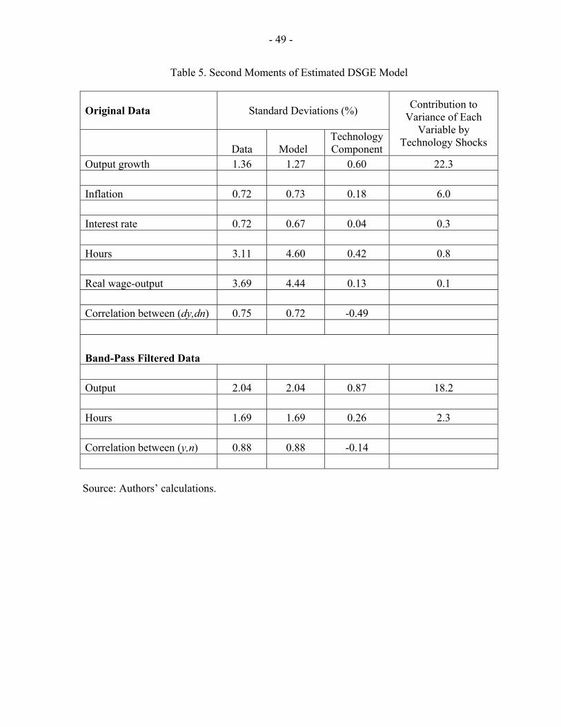
- 49 -

Table 5. Second Moments of Estimated DSGE Model

Source: Authors’ calculations.

Original Data

Standard Deviations (%)

Data Model Technology Component

Contribution to Variance of Each

Variable by Technology Shocks

Output growth 1.36 1.27 0.60 22.3 Inflation 0.72 0.73 0.18 6.0 Interest rate 0.72 0.67 0.04 0.3 Hours 3.11 4.60 0.42 0.8 Real wage-output 3.69 4.44 0.13 0.1 Correlation between (dy,dn) 0.75 0.72 -0.49

Band-Pass Filtered Data Output 2.04 2.04 0.87 18.2 Hours 1.69 1.69 0.26 2.3 Correlation between (y,n) 0.88 0.88 -0.14

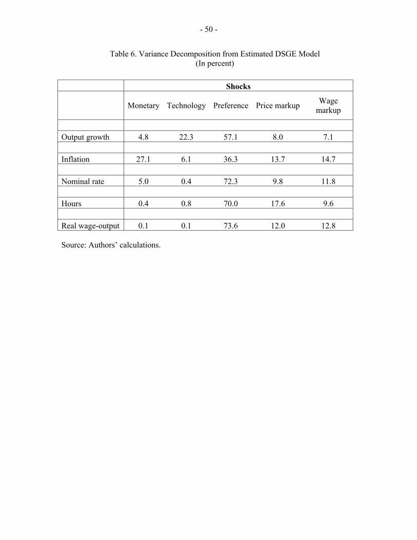
- 50 -

Table 6. Variance Decomposition from Estimated DSGE Model (In percent)

Source: Authors’ calculations.

Shocks

Monetary

Technology

Preference

Price markup Wage markup

Output growth 4.8 22.3 57.1 8.0 7.1 Inflation 27.1 6.1 36.3 13.7 14.7 Nominal rate 5.0 0.4 72.3 9.8 11.8 Hours 0.4 0.8 70.0 17.6 9.6 Real wage-output 0.1 0.1 73.6 12.0 12.8

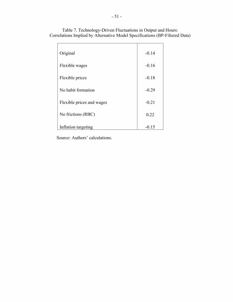
- 51 -

Table 7. Technology-Driven Fluctuations in Output and Hours: Correlations Implied by Alternative Model Specifications (BP-Filtered Data)

Original -0.14 Flexible wages -0.16 Flexible prices -0.18 No habit formation -0.29 Flexible prices and wages -0.21 No frictions (RBC) 0.22 Inflation targeting -0.15

Source: Authors’ calculations.

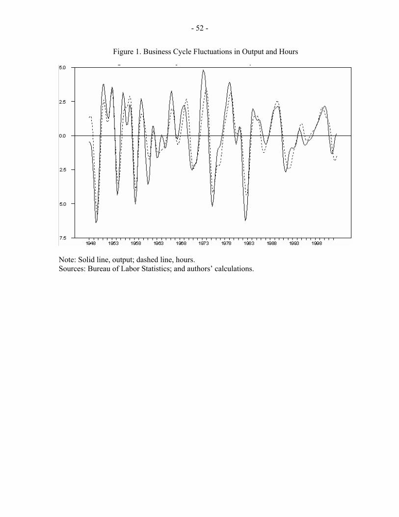
- 52 -

Figure 1. Business Cycle Fluctuations in Output and Hours

Note: Solid line, output; dashed line, hours. Sources: Bureau of Labor Statistics; and authors’ calculations.

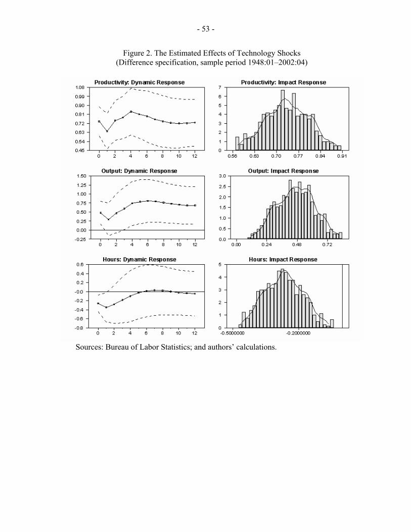
- 53 -

Figure 2. The Estimated Effects of Technology Shocks (Difference specification, sample period 1948:01–2002:04)

Sources: Bureau of Labor Statistics; and authors’ calculations.

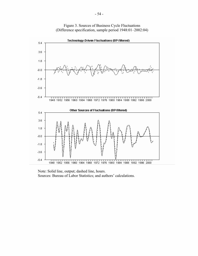
- 54 -

Figure 3. Sources of Business Cycle Fluctuations (Difference specification, sample period 1948:01–2002:04)

Note: Solid line, output; dashed line, hours. Sources: Bureau of Labor Statistics; and authors’ calculations.

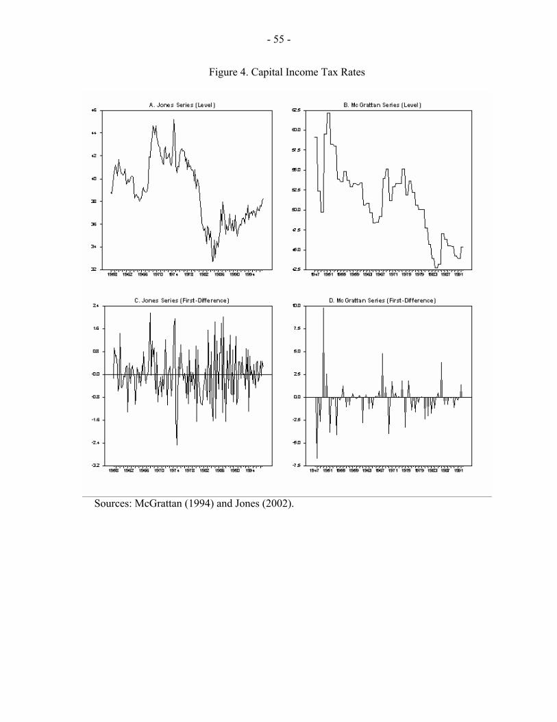
- 55 -

Figure 4. Capital Income Tax Rates

Sources: McGrattan (1994) and Jones (2002).

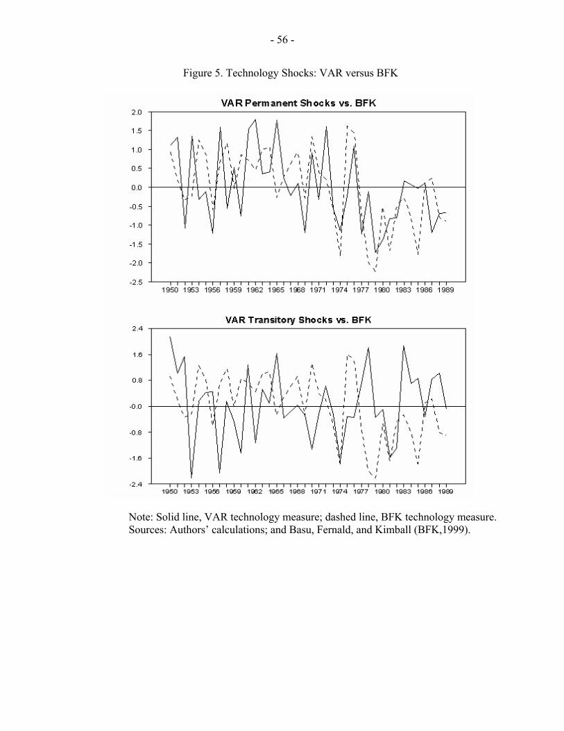
- 56 -

Figure 5. Technology Shocks: VAR versus BFK

Note: Solid line, VAR technology measure; dashed line, BFK technology measure. Sources: Authors’ calculations; and Basu, Fernald, and Kimball (BFK,1999).

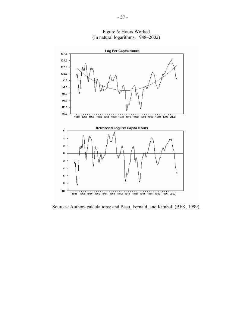
- 57 -

Figure 6: Hours Worked (In natural logarithms, 1948–2002)

Sources: Authors calculations; and Basu, Fernald, and Kimball (BFK, 1999).

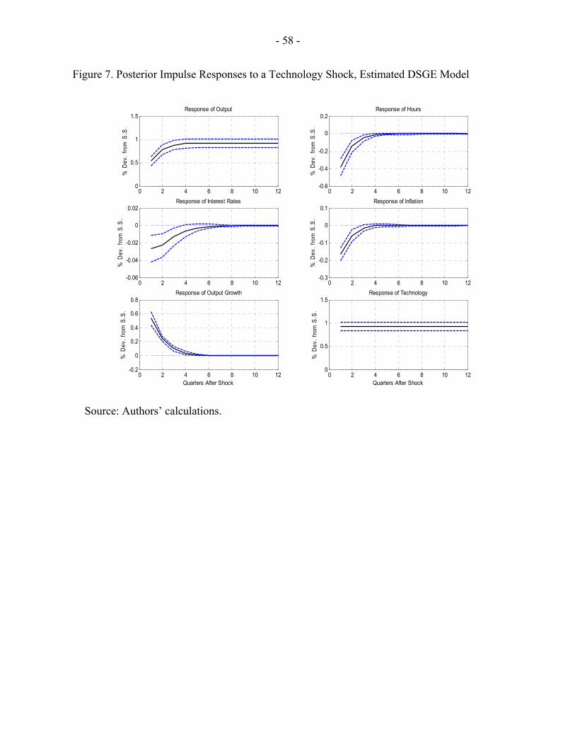
- 58 -

Figure 7. Posterior Impulse Responses to a Technology Shock, Estimated DSGE Model

0 2 4 6 8 10 120

0.5

1

1.5%

Dev

. fro

m S

.S.

Response of Output

0 2 4 6 8 10 12-0.6

-0.4

-0.2

0

0.2

% D

ev. f

rom

S.S

.

Response of Hours

0 2 4 6 8 10 12-0.06

-0.04

-0.02

0

0.02

% D

ev. f

rom

S.S

.

Response of Interest Rates

0 2 4 6 8 10 12-0.3

-0.2

-0.1

0

0.1

% D

ev. f

rom

S.S

.

Response of Inflation

0 2 4 6 8 10 12-0.2

0

0.2

0.4

0.6

0.8

Quarters After Shock

% D

ev. f

rom

S.S

.

Response of Output Growth

0 2 4 6 8 10 120

0.5

1

1.5

Quarters After Shock

% D

ev. f

rom

S.S

.

Response of Technology

Source: Authors’ calculations.

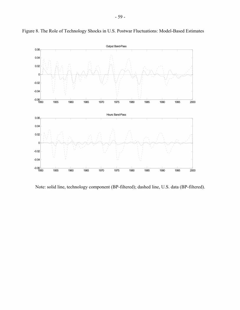
- 59 -

Figure 8. The Role of Technology Shocks in U.S. Postwar Fluctuations: Model-Based Estimates

1950 1955 1960 1965 1970 1975 1980 1985 1990 1995 2000-0.06

-0.04

-0.02

0

0.02

0.04

0.06Output Band-Pass

1950 1955 1960 1965 1970 1975 1980 1985 1990 1995 2000-0.06

-0.04

-0.02

0

0.02

0.04

0.06Hours Band-Pass

Note: solid line, technology component (BP-filtered); dashed line, U.S. data (BP-filtered).

- 60 -

REFERENCES

Altig, D., L. J. Christiano, M. Eichenbaum, and J. Linde, 2003, “Monetary Policy and the Dynamic Effects of Technology Shocks” (unpublished, Evanston: Northwestern University).

Basu, S., J. Fernald, and M. Kimball, 1999, “Are Technology Improvements

Contractionary?,” (unpublished, Ann Arbor: University of Michigan). Basu, S., and M. Kimball, 1997, “Cyclical Productivity with Unobserved Input Variation,”

NBER Working Paper 5915 (Cambridge: National Bureau of Economic Research). Baxter, M. and R. G. King, 1999, “Measuring Business Cycles: Approximate Band-Pass

Filters for Economic Time Series,” The Review of Economics and Statistics, 81(4), pp. 575–93.

Bils, M. and P. J. Klenow, 2002, “Some Evidence on the Importance of Sticky Prices,”

NBER Working Paper 9069 (Cambridge: National Bureau of Economic Research). Blanchard, O., 1989, “A Traditional Interpretation of Macroeconomic Fluctuations,”

American Economic Review, Vol. 79, No. 5, pp. 1146-64. Blanchard, O., and D. Quah, 1989, “The Dynamic Effects of Aggregate Demand and Supply

Disturbances,” American Economic Review, Vol. 79, No. 4, pp. 655-73. Blanchard, O., R. Solow, and B.A. Wilson, 1995, “Productivity and Unemployment”

(unpublished, Cambridge: Massachussets Institute of Technology). Boivin, J. and M, Giannoni, 2003, “Has Monetary Policy Become More Effective?” NBER

Working Paper 9459 (Cambridge: National Bureau of Economic Research). Bullard, J. and K. Mitra, 2002,”"Learning About Monetary Policy Rules”, Journal of

Monetary Economics, Vol. 49, No. 6, pp. 1105–129. Burnside, C., and M. Eichenbaum, 1996, “Factor Hoarding and the Propagation of Business

Cycle Shocks, American Economic Review, Vol. 86, No. 5, pp. 1154-74.

Burnside, C., M. Eichenbaum, and S. Rebelo, 1995, “Capital Utilization and Returns to Scale,” NBER Macroeconomics Annual 1995, Ben S. Bernanke and Julio J. Rotemberg,eds.,Cambridge: MIT Press, pp. 67-110.

Calvo, G., 1983, “Staggered Prices in a Utility Maximizing Framework,” Journal of

Monetary Economics, Vol. 12, No. 3, pp. 383–98. Campbell, J., 1994, "Inspecting the Mechanism: An Analytical Approach to the Stochastic

Growth Model," Journal of Monetary Economics, Vol .33, June, pp. 463-506

- 61 -

Carlsson, M., 2000, “Measures of Technology and the Short-Run Responses to Technology

Shocks: Is the RBC Model Consistent with Swedish Manufacturing Data?,” (unpublished, Uppsala, Sweden: University of Uppsala).

Chang, Y. and J.H. Hong, 2003, “On the Employment Effects of Technology: Evidence from

U.S. Manufacturing for 1958–96” (unpublished, Philadelphia: University of Pennsylvania).

Chari, V.V., P. J. Kehoe, and E. McGrattan,, 2004, “Are Structural VARs Useful Guides for

Developing Business Cycle Theories?,” FRB of Minneapolis Working Paper 631 (Minneapolis: Federal Reserve Bank of Minneapolis).

Christiano, L., M. Eichenbaum, and C. Evans, 2003, “Nominal Rigidities and the Dynamic

Effects of a Shock to a Monetary Policy”, Journal of Political Economy, forthcoming. Christiano, L., M. Eichenbaum, and R. Vigfusson, 2003, “What happens after a Technology

Shock?” (unpublished, Evanston: Northwestern University). ———, 2004, “The Response of Hours to a Technology Shock: Evidence Based on Direct

Measures of Technology,” EEA Meeting Papers and Proceedings, Journal of the European Economic Association (forthcoming).

Collard, F. and H. Dellas, 2002, “Technology Shocks and Employment” (unpublished,

Toulouse, France: Université de Toulouse). Cooley, T. F. and M. Dwyer, 1998, “Business Cycle Analysis Without Much Theory: A

Look at Structural VARs,” Journal of Econometrics, Vol. 83, No. 1, pp. 57–88. Cooley, T. F. and E.C. Prescott, 1995, “Economic Growth and Business Cycles,” Frontiers

of Business Cycle Research (Princeton: Princeton University Press). Cummins, J. and G. Violante, 2002, “Investment-Specific Technical Change in the United

States (1947–2000),” Review of Economic Dynamics, Vol. 5, No. 2, pp. 243–84. Dotsey, M., 2002, “Structure from Shocks,” Economic Quarterly, Vol. 88, No. 4, pp. 1–13,

Federal Reserve Bank of Richmond. Erceg, C.J., L. Guerrieri, and C. Gust, 2004, “Can Long Run Restrictions Identify

Technology Shocks?,” Federal Reserve Board Working Paper 792. Erceg, C.J. and A. Levin, 2003, “Imperfect Credibility and Inflation Persistence,” Journal of

Monetary Economics, Vol. 50, No 4, pp. 915–44. Fernald, J., 2004, “Trend Breaks, Long Run Restrictions, and the Contractionary effects of a

Technology Shock” (unpublished, Chicago: Federal Reserve Bank).

- 62 -

Fernández-Villaverde, J. and J.F. Rubio-Ramírez, 2004, “Comparing Dynamic Equilibrium

Economies to Data: A Bayesian Approach,” Journal of Econometrics, forthcoming. Fisher, J., 2003, “Technology Shocks Matter,” (unpublished; Chicago: Federal Reserve

Bank). Francis, N., 2001, “Sectoral Technology Shocks Revisited,” (unpublished manuscript;

Bethlehem, Pennsylvania: Lehigh University). Francis, N.R., M.T. Owyang, and A.T. Thedorou, ,2003, “The Use of Long Run Restrictions

for the Identification of Technology Shocks,” Federal Reserve Bank of St. Louis Review, November-December, pp. 53–66.

———, 2004, “What explains the Varying Monetary Response to Technology Shocks in G-7

Countries?,” (unpublished, Bethlehem: Lehigh University). Francis, N. and Valerie Ramey, 2003a, “Is the Technology-Driven Real Business Cycle

Hypothesis Dead? Shocks and Aggregate Fluctuations Revisited” (unpublished, San Diego: University of California).

———, 2003b, “The Source of Historical Economic Fluctuations: An Analysis using Long-

Run Restrictions” (unpublished, San Diego: University of California). Franco, F., and T. Philippon, 2004, “Industry and Aggregate Dynamics” (unpublished,

Cambridge: Massachussets Institute of Technology). Galí, J., 1998, "What Do Technology Shocks Do? A Comment?," NBER Macroeconomics

Annual 1998, Bernanke, Ben and Julio Rotemberg, eds., Cambridge: MIT Press, pp. 310-316.

———, 1999, “Technology, Employment, and the Business Cycle: Do Technology Shocks

Explain Aggregate Fluctuations?,” American Economic Review, Vol. 89, No. 1, pp. 249–71.

———, 2003, “New Perspectives on Monetary Policy, Inflation, and the Business Cycle,” in

Advances in Economics and Econometrics, Volume III, edited by M. Dewatripont, L. Hansen, and S. Turnovsky (Cambridge: Cambridge University Press).

———, 2004, “On the Role of Technology Shocks as a Source of Business Cycles: Some

New Evidence,” Journal of the European Economic Association, forthcoming. ———, and Mark Gertler, 1999, “Inflation Dynamics: A Structural Econometric Analysis,”

Journal of Monetary Economics, Vol. 44, No. 2, pp. 195–222.

- 63 -

Galí, J, J. D. López-Salido, and J.Vallés, 2003, “Technology Shocks and Monetary Policy: Assessing the Fed's Performance,” Journal of Monetary Economics, Vol. 50, No. 4, pp. 723–43.

Gordon, R., 1990, “The Measurement of Durable Goods Prices” (Chicago: University of

Chicago Press). Greenwood, J., Z. Hercowitz, and G.W. Huffman, 1998, “Investment, Capacity Utilization,

and the Real Business Cycle,” American Economic Review, Vol. 78, No. 3, pp. 402–17.

Greenwood, J., Z. Hercowitz, and P. Krusell, 1997, “Long-Run Implications of Investment

Specific Technological Change,” American Economic Review, Vol 87, pp. 342–362. ———, 2000, “The Role of Investment-Specific Technical Change in the Business Cycle,”

European Economic Review, Vol 44, pp. 91–115. Hall, R.E,. 1988, “The Relation Between Price and Marginal Cost in U.S. Industry,” Journal

of Political Economy 96, pp. 921–47. Hamilton, J., 1994, Time Series Analysis, Princeton University Press. Hoover, K., and S.J. Perez, 1994, “Post Hoc Ergo Procter Once More: An Evaluation of

‘Does Monetary Policy Matter?’ in the Spirit of James Tobin,” Journal of Monetary Economics, Vol. 34, Issue 1, pp. 47–74.

Ingram, B., N. Kocherlakota, and N.E. Savin, 1994, “Explaining Business Cycles: A

Multiple-shock Approach,” Journal of Monetary Economics, Vol. 34, Issue 3, pp. 415–28 (December).

Ireland, P., 2004, “Technology Shocks in the New Keynesian Model”, (unpublished, Boston:

Boston College). Jones, J.B., 2002, “Has Fiscal Policy Helped Stabilize the U.S. Economy?,” Journal of

Monetary Economics, Vol 49, No. 4, pp. 709–46. Kiley, M.T., 1997, “Labor Productivity in U.S. Manufacturing: Does Sectoral Comovement

Reflect Technology Shocks?” (unpublished, Washington: Federal Reserve Board). King, R., C. Plosser, and S. Rebelo, 1988a, “Production, Growth and Business Cycles I: The

Basic Neoclassical Model,” Journal of Monetary Economics, Vol. 21, March/May, pp. 195-232.

———, 1988b, “Production, Growth and Business Cycles II: New Directions,” Journal of Monetary Economics, Vol. 21, March/May, pp. 309-341.

- 64 -

King, R.G., and S.T. Rebelo, 1999, “Resuscitating Real Business Cycles,” in J.B. Taylor and

M. Woodford (eds.) Handbook of Macroeconomics, Vol. 1B, pp. 928–1002 (also National Bureau of Economic Research Working Paper 7534).

Kwiatkowski, D., P.C.B. Phillips, P. Schmidt and Y. Shin, 1992, “Testing the Null

Hypothesis of Stationarity Against the Alternative of a Unit Root,” Journal of Econometrics, Vol. 54, pp. 159-178.

Kydland, F.E. and E.C. Prescott, 1982, “Time to Build and Aggregate Fluctuations,”

Econometrica, Vol. 50, No. 6 ,pp. 1345–70. Lettau, M. and H. Uhlig, 2000, “Can Habit Formation be Reconciled with Business Cycle

Facts?,” Review of Economic Dynamics, Vol. 3, No. 1, pp. 79–99. Lubik, T. and F. Schorfheide, 2003, “Testing for Indeterminacy: An Application to U.S.

Monetary Policy,” American Economic Review, Vol. 94, no. 1, pp. 190-217 ———, 2004, “Do Central Banks Respond to Exchange Rates? A Structural Investigation?”

(unpublished, Philadelphia: University of Pennsylvania). Marchetti, D.J., and F. Nucci ,2004, “Price Stickiness and the Contractionary Effects of

Technology Shocks,” European Economic Review, forthcoming. Marcet, A., 2004, “Overdifferencing VAR's is OK” (unpublished, Barcelona, Spain:

Universitat Pompeu Fabra). McGrattan, E., 1994, “The Macroeconomic Effects of Distortionary Taxation,” Journal of

Monetary Economics, Vol. 33, No. , pp. 573–601. ———, 1999, “Predicting the Effects of Federal Reserve Policy in a Sticky-Price Model,”

FRB Working Paper 598 (Minneapolis: Federal Reserve Bank). ———, 2004, “Comment to Galí and Rabanal”, in Mark Gertler and Ken Rogoff (eds.),

NBER Macroeconomics Annual 2004, in press. Orphanides, A. and J. Williams, 2002, “Robust Monetary Policy Rules with Unknown

Natural Rates,” Brookings Papers on Economic Activity, Vol. 2002, pp. 63–118 (Washington: Brookings Institutions).

Pesavento, E. and B. Rossi, 2003, “Do Technology Shocks Drive Hours Up or Down: A

Little Evidence from an Agnostic Procedure” (unpublished, Durham: Duke University).

Prescott, E.C., 1986a, “Theory Ahead of Business Cycle Measurement,” Quarterly

Review 10, pp. 9–22, Federal Reserve Bank of Minneapolis.

- 65 -

———, 1986b, “Response to a Skeptic,” Quarterly Review 10, pp. 28–33 (Minneapolis:

Federal Reserve Bank). Rabanal, P., 2003, “The Cost Channel of Monetary Policy: Further Evidence for the United

States and the Euro Area,” IMF Working Paper 03/149 (Washington: International Monetary Fund).

Ramey, V., and M.D. Shapiro, 1998, “Costly Capital Reallocation and the Effects of

Government Spending,” Carnegie-Rochester Conference Series on Public Policy, Vol. 48, pp. 145–194.

Romer, C., and D. Romer, 1989, “Does Monetary Policy Matter? A Test in the Spirit of

Friedman and Schwartz,” NBER Macroeconomics Annual 1998, Bernanke, Ben and Julio Rotemberg, eds., Cambridge: MIT Press, pp. 63–129.

Rotemberg, J.J., 2003, “Stochastic Technical Progress, smooth Trends, and Nearly Distinct

Business Cycles,” American Economic Review, Vol. 93, No. 5, pp. 1543–59. Rotemberg, J.J., and M. Woodford, 1999, “Interest Rate Rules in an Estimated Sticky Price

Model,” in Monetary Policy Rules, J.B. Taylor (ed.), Chicago: University of Chicago Press.

Shea, J., 1998, "What Do Technology Shocks Do?," NBER Macroeconomics Annual 1998,

Bernanke, Ben and Julio Rotemberg, eds., Cambridge: MIT Press, pp. 275-310. Smets, F. and R. Wouters, 2003a, “An Estimated Stochastic Dynamic General Equilibrium

Model of the Euro Area,” Journal of the European Economic Association, Vol 1 (5), pp. 1123–75.

———, 2003b, “Shocks and Frictions in U.S. Business Cycles: A Bayesian DSGE

Approach” (unpublished; Frankfurt: European Central Bank). Solow, R., 1957, “Technical Change and the Aggregate Production Function,” Review of

Economics and Statistics, Vol. 39, pp. 312–20. Stock, J., and M.W. Watson, 1999, “Business Cycle Fluctuations in U.S. Macroeconomic

Time Series,” in J.B. Taylor and M. Woodford (eds.), Handbook of Macroeconomics, Volume 1A, pp. 3–64 (see also National Bureau of Economics Research Working Paper 6528).

Taylor, J.B., 1993, “Discretion versus Policy Rules in Practice,” Carnegie-Rochester Series

on Public Policy, Vol. 39, pp. 195–214.

- 66 -

Uhlig, H., 1999, “A Toolkit for Analyzing Nonlinear Dynamic Stochastic Models Easily,” in Computational Methods for the Study of Dynamic Economies, edited by Ramon Marimon and Andrew Scott (Oxford: Oxford University Press).

———, 2004, “Do Technology Shocks Lead to a Fall in Total Hours Worked?” Journal of

the European Economic Association, forthcoming. Wen, Y., 2001, “Technology, Employment and the Business Cycle: Do Technology Shocks

Explain Aggregate Fluctuations? A Comment”. Cornel University Working Paper No. 01-19 (Ithaca, NY: Cornell University).