Embed Size (px)
Citation preview

AC 2012-3164: TEACHING MULTIBODY SYSTEM SIMULATION: ANAPPROACH WITH MATLAB
Dr. Peter Wolfsteiner, Munich University of Applied Sciences
Peter Wolfsteiner is professor in mechanical engineering at the Munich University of Applied Sciences(HM) in Germany. He received his Ph.D. degree in M.E. from the Technical University Munich. Prior tojoining the faculty at HM, he worked at Knorr-Bremse Group as a Manager in the area of new technologiesfor rail vehicle braking systems. He teaches undergraduate and graduate courses in statics, strength ofmaterials, dynamics, controls, numerics, and simulation of dynamical systems. Research interests includesimulation, nonlinear dynamics, random vibrations, and fatigue. He is currently working as exchangeprofessor at California Polytechnic State University in San Luis Obispo.
c©American Society for Engineering Education, 2012
Page 25.1252.1
Teaching Multibody System Simulation, an Approach with
MATLAB
Abstract
Teaching Multibody Systems needs to cover the related theoretical concepts of advanceddynamics, the application of the necessary numerical methods in a sufficient depth, andneeds to give students the opportunity to model and solve authentic problems on theirown. The last step may only be done with the help of a computer. A variety of highlysophisticated computer programs are available (e.g., Adams), able to solve special problemsfrom the area of Multibody Systems or even nearly every general type of engineeringdynamics problem. The use of such software has some drawbacks for students however.There is a high risk to waste valuable time by learning how to use software that was notdesigned for educational use but was instead designed for large scale problems in industry.And, what is even worse, students do not really see how the software works, because thetransition from the theoretical to numerical concepts is usually not visible in the software.To deal with this challenge, this paper presents a strategy based on the software Matlab,usually known by engineering students. The proposed method is based on doing symbolicmanipulations for the derivations of the equations and on using numerical methods for thesolution. The main idea is not to waste time and effort for getting the equations in a certainform needed for a computer solution, but to offer a procedure allowing students to easilyuse the equations as they are -known from the theoretical concept- and directly use them inMatlab. Furthermore the intention is not to be limited to simple 2D problems with just afew degrees of freedom but to offer the full range of a 3D Multibody System simulation withmodelling, derivation of equations of motion, numerical solution of differential equations,calculation of static equilibrium as well as linearization and calculation of eigenvalues andeigenmodes. Based on a couple of small examples the paper gives a detailed introduction tothe proposed method including all necessary equations and also the related Matlab code.
1 Introduction
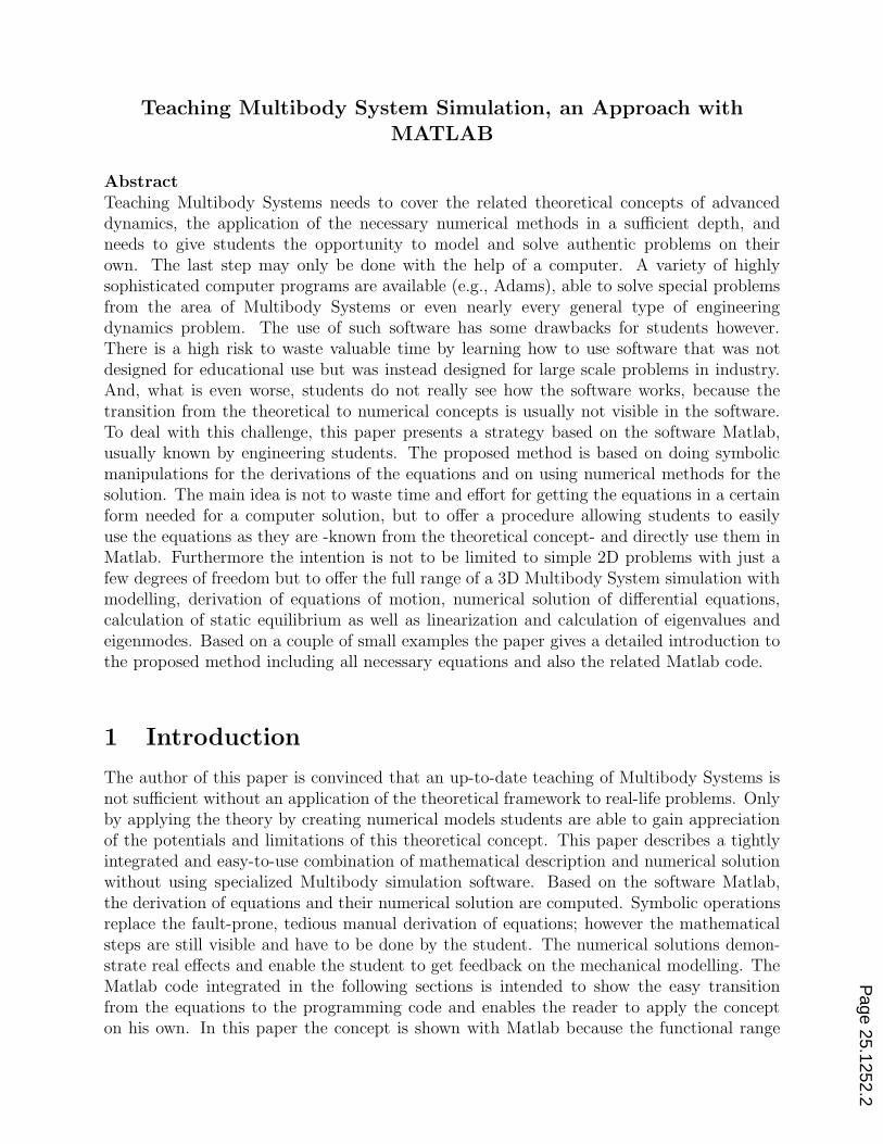
The author of this paper is convinced that an up-to-date teaching of Multibody Systems isnot sufficient without an application of the theoretical framework to real-life problems. Onlyby applying the theory by creating numerical models students are able to gain appreciationof the potentials and limitations of this theoretical concept. This paper describes a tightlyintegrated and easy-to-use combination of mathematical description and numerical solutionwithout using specialized Multibody simulation software. Based on the software Matlab,the derivation of equations and their numerical solution are computed. Symbolic operationsreplace the fault-prone, tedious manual derivation of equations; however the mathematicalsteps are still visible and have to be done by the student. The numerical solutions demon-strate real effects and enable the student to get feedback on the mechanical modelling. TheMatlab code integrated in the following sections is intended to show the easy transitionfrom the equations to the programming code and enables the reader to apply the concepton his own. In this paper the concept is shown with Matlab because the functional range
Page 25.1252.2

(operations with vectors/matrices, symbolic and numerical tools, plentiful numerical rou-tines) of this software meets the needs very well. Similar software tools (e.g.: MAPLE,MATHEMATICA) may also be applied.The approach to the Multibody subject in literature is manifold and varies in structureand notation. The concept used here is derived from1,2,3 and may easily be adapted toalternative concepts. Also the profitable use of numerical tools like Matlab in engineeringeducation is well known and many different proposals have been widely discussed in a highnumber of publications for lots of different fields of engineering activity. However, usefulcombinations of symbolical and numerical tools for engineering applications seem not yet tobe so much accepted. The idea of combining both in Matlab for dynamics is taken from4 , thespecial focus on Multibody Systems shown here seems to be not yet available in engineeringeducation literature.This paper does not intend to explain Multibody system theory nor the basic applicationof Matlab. A basic knowledge in these fields is assumed to be known. The paper also doesnot explain the details of the mathematical derivations nor the Matlab code. It is assumedthat the examples are self-explanatory if they are worked through. The paper keeps its focuson demonstrating the educational concept with some selected ’academic’ examples. Theyare chosen with the idea to be as simple as possible, but also able to show the capability ofthe proposed method. They are part of a complete Multibody Systems teaching concept forgraduate students consisting of lectures with a script provided by the lecturer, homeworkproblems giving an opportunity to practice theoretical skills and lab assignments based on theuse of Matlab as shown in this paper (the knowledge of the Matlab programming languageis a prerequisite for this class). Therefore students usually develop code on their own basedon code examples demonstrating the basic concepts. These code examples also include aselection of library functions providing, for example, an animation function that can be usedto demonstrate the results with a small movie. Figure 1 shows some (animation-) examplesthat have been covered within this class.
0 1 2 3
0
0.5
1
1.5
2
2.5
3
3.5
4
X−Achse
Y−
Ach
se
−0.4
−0.2
0
0.2
0.4
0.6
0.8−0.5
−0.4
−0.3
−0.2
−0.1
0
0.1
0.2
0.3
0.4
0.5
0
0.1
0.2
0.3
Z−
Ach
se
X−Achse
Y−Achse −0.5 0 0.5
−2
−1.5
−1
−0.5
0
0.5
1
X−Achse
Y−
Ach
se
Vehicle Suspension Tricycle Dynamics Reciprocating Engine
Figure 1: Examples of Modelled Multibody Systems
The approach has been developed by the author over the last five years and was successfullyapplied to graduate students at a German university of applied sciences within a mastersprogram focused on Mechatronics. This program is job-oriented and tries to teach pro-fessional skills. The Mechatronics concentration requires a strong emphasis on dynamics,
Page 25.1252.3
modelling, controls, simulations and the application of related software. The use of Matlabfor Multibody Systems tries to serve this need. The student feedback on this class usuallyshows the following three major points:
very demanding: starting with pure dynamics theory and ending with programmingnumerical algorithms a wide range of skills is required,
highly satisfying: students get very satisfied by obtaining the ability to solve real lifenonlinear dynamics problems on their own by applying elementary dynamics theorywithout the help of special dynamics software tools,
good integration in Mechatronics: the ability to model and analyze dynamicsproblems in Matlab fits very well into a framework of a Mechatronics Masters pro-gram which also includes controls and signal analysis in Matlab.
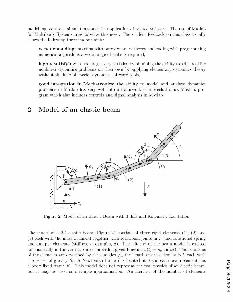
2 Model of an elastic beam
Figure 2: Model of an Elastic Beam with 3 dofs and Kinematic Excitation
The model of a 2D elastic beam (Figure 2) consists of three rigid elements (1), (2) and(3) each with the mass m linked together with rotational joints in Pi and rotational springand damper elements (stiffness c, damping d). The left end of the beam model is excitedkinematically in the vertical direction with a given function u(t) = uo sin(ωt). The rotationsof the elements are described by three angles ϕi, the length of each element is l, each withthe center of gravity Si. A Newtonian frame I is located at 0 and each beam element hasa body fixed frame Ki. This model does not represent the real physics of an elastic beam,but it may be used as a simple approximation. An increase of the number of elements
Page 25.1252.4

improves the quality of approximation to the real behavior. However in this simple formthe model is sufficient to demonstrate a couple of typical tasks relevant to the operationwith Multibody problems. The following sections explain the derivation of the equations ofmotion. Because of its compact theoretical formulation section 2.1 starts with the Lagrangeequation of second kind, section 2.2 demonstrates the more relevant procedure with theNewton-Euler equations.
2.1 Lagrange equation of second kind
For the derivation of equations of motion this section uses the Lagrange equation of secondkind with the vector of minimal coordinates q = (ϕ1, ϕ2, ϕ3)
T , the kinetic energy T , thepotential energy V and the vector of generalized forces u:
d
dt
(
∂T
∂q
)
−∂T
∂q+
∂V
∂q= uT . (1)
The kinetic energy T may be derived for one beam element i with respect to the center ofgravity Si with Equation 2:
Ti =1
2m vT
SivSi
+1
2ωT
i I(Si)i ωi, (2)
with the mass mi, the inertia tensor I(S)i , the velocity vSi
and the angular velocity ωi.The potential energy of the weight forces (index i) and the spring moments (index j) withEquation 3:
Vi = −mi gT rOSi; Vj =
c
2ϕ2
rel,j. (3)
The nonpotential moments (index j) on body i caused by the dampers are presented asEquation 4:
mj = d ϕrel,j ; uij =
(
∂ϕi
∂q
)T
mj. (4)
These equations allow the derivation of the equations of motion in the following form byperforming the derivatives of Equation 1:
M(t, q) q − h(t, q, q) = 0. (5)
The following steps describe the implementation in Matlab.
Symbolic Derivation of Equations of Motion: Listing 1 shows the first section of theMatlab code used for deriving the equations of motion with the above set of equations. Table1 explains the code.
Numerical Evaluation of Symbolic Expressions: The numerical analysis of the equa-tions of motion requires a numerical evaluation of the derived symbolic expressions for M
and h. For this purpose Matlab offers the command subs that performs a substitution ofsymbolic expressions with numerical ones. But the application of the subs command within
Page 25.1252.5

Table 1: Description of Listing 1line: code:
1 to 5 setting of parameters, the inertia tensor is: I(S)i =
0 0 00 0 00 0 m
12l2
7 to 9 definition of symbolic variables necessary for the following derivations (phi1 →
ϕ1, phi1_p → ϕ1, ...)11 to 28 derivation of kinematics:
• the notation of the vector K1rP1P2
(in Matlab: K1_r_P1P2) denotes thevector r pointing from P1 to P2 noted in the frame K1,
• the function A_z(phi) is a separate function calculating the transforma-
tion matrix AIK(ϕ) =
cos ϕ − sin ϕ 0sin ϕ cos ϕ 0
0 0 1
for a rotation of K with
respect to the frame I about the axis Z with the angle ϕ,
• the velocities IvSiof the centers of gravity are calculated with the
time derivatives of the position vectors IvSi= I rSi
, since t is not ex-pressed explicitly in IrOSi
(t, q), the time derivative is calculated withr = d
dtr(t, q) = ∂r
∂q q + ∂r∂t
,
30 to 33 kinetic energy corresponding to Equation 235 to 37 potential energy corresponding to Equation 339 to 45 generalized forces corresponding to Equation 447 to 51 derivation of equations of motion (Equation 5) corresponding to Equation 1:
• since t is not expressed explicitly in T and V , the time derivatives are
calculated symbolically with: ddt
(
∂T
∂q
)T
= ∂
∂q
(
∂T
∂q
)T
q + ∂∂q
(
∂T
∂q
)T
q +
∂∂t
(
∂T
∂q
)T
,
• M(t, q) = ∂
∂q
(
∂T
∂q
)T
,
• h(t, q, q) = −∂
∂q
(
∂T
∂q
)T
q −∂∂t
(
∂T
∂q
)T
+(
∂T∂q
)T−
(∂V∂q
)T+ u,
the framework of numerical integration shows that the computational effort is even for smallequations very high, with the consequence of long simulation times. It seems that the callof subs launches the symbolic toolbox every time subs is called, doing lots of inefficientcomputations! To solve this problem, the author uses the self developed routine sym_2_fun
that generates a callable Matlab-function from a symbolic expression (see Listing 2). In
Page 25.1252.6

Listing 1: Symbolic Derivation of Equations of Motion with Lagrange Equation of SecondKind1 % parameters :2 g = [ 0 ; − 9 . 8 1 ; 0 ] ; m = 1 ;3 l = 1 ; c r o t = 100 ; d rot = 3 ;4 omega 0 = 5∗2∗ pi ; u 0 = . 1 ;5 K I S = [ 0 0 0 ; 0 0 0 ; 0 0 m∗ l ˆ 2/12 ] ;6
7 % d e f i n i t i o n s :8 syms phi1 phi2 phi3 phi1 d phi2 d phi3 d t9 q = [ phi1 ; phi2 ; phi3 ] ; q d = [ phi1 d ; phi2 d ; phi3 d ] ; x = [ q ; q d ] ;
10
11 % kinemat i c s :12 K1 r P1P2 = [ l ; 0 ; 0 ] ; K2 r P2P3 = [ l ; 0 ; 0 ] ;13 K1 r P1S1 = [ l / 2 ; 0 ; 0 ] ; K2 r P2S2 = [ l / 2 ; 0 ; 0 ] ; K3 r P3S3 = [ l / 2 ; 0 ; 0 ] ;14 A IK1 = A z ( phi1 ) ; A IK2 = A z ( phi2 ) ; A IK3 = A z ( phi3 ) ;15
16 I r 0P1 = [ 0 ; u 0 ∗ s i n ( omega 0∗ t ) ; 0 ] ;17 I r 0P2 = I r 0P1 + A IK1∗K1 r P1P2 ;18 I r 0P3 = I r 0P2 + A IK2∗K2 r P2P3 ;19 I r 0S1 = I r 0P1 + A IK1∗K1 r P1S1 ;20 I r 0S2 = I r 0P2 + A IK2∗K2 r P2S2 ;21 I r 0S3 = I r 0P3 + A IK3∗K3 r P3S3 ;22
23 I v S1 = jacob ian ( I r 0S1 , q )∗ q d + d i f f ( I r 0S1 , t ) ;24 I v S2 = jacob ian ( I r 0S2 , q )∗ q d + d i f f ( I r 0S2 , t ) ;25 I v S3 = jacob ian ( I r 0S3 , q )∗ q d + d i f f ( I r 0S3 , t ) ;26 K1 omega IK1 = [ 0 ; 0 ; phi1 d ] ;27 K2 omega IK2 = [ 0 ; 0 ; phi2 d ] ;28 K3 omega IK3 = [ 0 ; 0 ; phi3 d ] ;29
30 % k i n e t i c energy :31 T =(m∗ I v S1 . ’ ∗ I v S1 + K1 omega IK1 . ’ ∗ K I S∗K1 omega IK1 + . . .32 m∗ I v S2 . ’ ∗ I v S2 + K2 omega IK2 . ’ ∗ K I S∗K2 omega IK2 + . . .33 m∗ I v S3 . ’ ∗ I v S3 + K3 omega IK3 . ’ ∗ K I S∗K3 omega IK3 )/2 ;34
35 % po t en t i a l energy :36 V = c r o t /2∗( phi1 ˆ2 + ( phi2−phi1 )ˆ2 + ( phi3−phi2 )ˆ2 ) − . . .37 m∗g . ’ ∗ ( I r 0S1 + I r 0S2 + I r 0S3 ) ;38
39 % non−po t en t i a l f o r c e s ( r ot . dampers ) :40 m p1 = ( phi1 d )∗ d rot ;41 m p2 = ( phi2 d−phi1 d )∗ d rot ;42 m p3 = ( phi3 d−phi2 d )∗ d rot ;43 u = jacob ian ( phi1 , q ) . ’ ∗ ( m p2−m p1 )+ . . .44 j acob ian ( phi2 , q ) . ’ ∗ ( m p3−m p2 )+ . . .45 j acob ian ( phi3 , q ) . ’ ∗ ( −m p3 ) ;46
47 % equat i ons o f motion :48 M = s imp l i f y ( j acob ian ( j acob ian (T, q d ) . ’ , q d ) ) ;49 h = s imp l i f y(− j acob ian ( j acob ian (T, q d ) . ’ , q )∗ q d . . .50 −j acob ian ( j acob ian (T, q d ) . ’ , t ) . . .51 +jacob ian (T, q ) . ’ −j acob ian (V, q ) . ’ + u ) ;
a first step the routine coo_2_vec replaces the elements of the state vector x (phi1, phi2,phi3, phi_1, phi_2, phi_3) by the array x(1:6), this makes the application of the generatedroutine easier. In the second step a Matlab-function is generated with the input variables xand t. The name of the generated function is stored in the variables f.M and f.h. Listing 2shows the procedure for M (t, q) and h(t, q, q) (lines 7 and 8). The functions generated forthe positions and rotations (lines 1 to 6) are needed later for the animation of the results.
Page 25.1252.7

The functions in line 9 and 10 are needed for the calculation of the static equilibrium andthe numerical integration. The transition from symbolic to numeric calculations is done herewith M(t, q) and h(t, q, q), although the expression M−1h is needed within the numericalintegration (see Numerical Integration). This is because the symbolic inversion of M is anextensive operation and produces a very large symbolic expression.
Listing 2: Derivation of Function Handles1 f . r o t {1} = sym 2 fun ( coo 2 vec (A IK1 , x ) , ’x , t ’ ) ;2 f . r o t {2} = sym 2 fun ( coo 2 vec (A IK2 , x ) , ’x , t ’ ) ;3 f . r o t {3} = sym 2 fun ( coo 2 vec (A IK3 , x ) , ’x , t ’ ) ;4 f . pos {1} = sym 2 fun ( coo 2 vec ( I r 0P1 , x ) , ’ x , t ’ ) ;5 f . pos {2} = sym 2 fun ( coo 2 vec ( I r 0P2 , x ) , ’ x , t ’ ) ;6 f . pos {3} = sym 2 fun ( coo 2 vec ( I r 0P3 , x ) , ’ x , t ’ ) ;7 f . h = sym 2 fun ( coo 2 vec (h , x ) , ’x , t ’ ) ;8 f .M = sym 2 fun ( coo 2 vec (M, x ) , ’x , t ’ ) ;9 f . ode f cn = @ode fcn ;
10 f . equ f cn = @e l a s t i c b eam equ i l i b r i um f cn ;
Animation: To make the interpretation of the results easier, the author uses a self de-veloped animation routine (animation), capable of demonstrating the motion of predefined3d-wireframe models on the screen within a Matlab figure. The definition of the bodies usedin the current example is shown in Listing 3. The animation is applied later for the staticequilibrium, the eigenmodes and the numerical integration (see Listing 4, 6, 7). The routineand its interface will not be explained in detail here.
Listing 3: Definitions for the Animation1 body = wi r e f r ame r e c tang l e xy ( l , l / 10 ) ;2 body {1} . geometry = w i r e f r ame o f f s e t ( body , [ l / 2 ; 0 ; 0 ] ) ; body {1} . c o l o r =1;3 body {2} . geometry = body {1} . geometry ; body {2} . c o l o r =2;4 body {3} . geometry = body {1} . geometry ; body {3} . c o l o r =3;
Static Equilibrium: Listings 4 and 5 show the code used for calculating the static equi-librium. The equation
h(t = 0, qo, q = 0) = 0 (6)
(see Listing 5, Line 2) defines a nonlinear set of equations, whose solution vector containsthe angles qo = (ϕ1o, ϕ2o, ϕ3o)
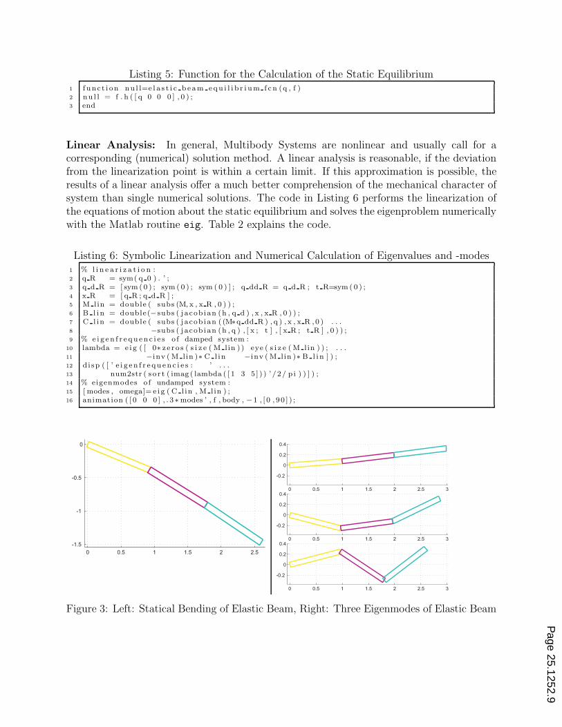
T of the static equilibrium. The Matlab function fsolve isused to find a numerical solution of the nonlinear equations. The function animation showsthe result on the screen (see Figure 3, left).
Listing 4: Numerical Calculation of Static Equilibrium1 q s t a r t = [ 0 0 0 ] ;2 q 0 = f s o l v e ( f . equ fcn , q s ta r t , [ ] , f ) ;3 animation (0 , q 0 , f , body , 0 , [ 0 , 9 0 ] ) ;
Page 25.1252.8
Listing 5: Function for the Calculation of the Static Equilibrium1 f unc t i on nu l l=e l a s t i c b e am equ i l i b r i um f cn (q , f )2 nu l l = f . h ( [ q 0 0 0 ] , 0 ) ;3 end
Linear Analysis: In general, Multibody Systems are nonlinear and usually call for acorresponding (numerical) solution method. A linear analysis is reasonable, if the deviationfrom the linearization point is within a certain limit. If this approximation is possible, theresults of a linear analysis offer a much better comprehension of the mechanical character ofsystem than single numerical solutions. The code in Listing 6 performs the linearization ofthe equations of motion about the static equilibrium and solves the eigenproblem numericallywith the Matlab routine eig. Table 2 explains the code.
Listing 6: Symbolic Linearization and Numerical Calculation of Eigenvalues and -modes1 % l i n e a r i z a t i o n :2 q R = sym( q 0 ) . ’ ;3 q d R = [ sym ( 0 ) ; sym ( 0 ) ; sym ( 0 ) ] ; q dd R = q d R ; t R=sym ( 0 ) ;4 x R = [ q R ; q d R ] ;5 M lin = double ( subs (M, x , x R , 0 ) ) ;6 B l i n = double(−subs ( j acob ian (h , q d ) , x , x R , 0 ) ) ;7 C l in = double ( subs ( j acob ian ( (M∗q dd R ) , q ) , x , x R , 0 ) . . .8 −subs ( j acob ian (h , q ) , [ x ; t ] , [ x R ; t R ] , 0 ) ) ;9 % e i g en f r e qu en c i e s o f damped system :
10 lambda = e i g ( [ 0∗ z e r o s ( s i z e ( M lin ) ) eye ( s i z e ( M lin ) ) ; . . .11 −inv ( M lin )∗ C l in −inv ( M lin )∗ B l i n ] ) ;12 di sp ( [ ’ e i g e n f r e qu en c i e s : ’ . . .13 num2str ( s o r t ( imag ( lambda ( [ 1 3 5 ] ) ) ’ / 2/ p i ) ) ] ) ;14 % eigenmodes o f undamped system :15 [ modes , omega]= e i g ( C l in , M lin ) ;16 animation ( [ 0 0 0 ] , . 3 ∗ modes ’ , f , body , −1 , [ 0 , 90 ] ) ;
Figure 3: Left: Statical Bending of Elastic Beam, Right: Three Eigenmodes of Elastic Beam
Page 25.1252.9

Table 2: Description of Listing 6line: code:
1 to 4 definition of reference motion (index R): the position is the static equilibrium(qR = qo), velocity, acceleration and time are set to zero (qR = qR = 0, tR = 0),for the following subs command these variables have to be defined symbolically!
5 to 8 the deviations from the reference motion (q = qR +y, q = qR + y, q = qR + y)are linearized with a taylor series, the resulting linear differential equation is:M(t) y + B(t) y + C(t) y = 0:
• M(q, t) q ≈ M(qR, t) qR +∂(M (q, t) q)
∂q
∣∣∣∣R
y(t) +∂(M (q, t) q)
∂q
∣∣∣∣R
y(t)
• h(q, q, t) ≈ h(qR, qR, t) +∂h(q, q, t)
∂q
∣∣∣∣R
y(t) +∂h(q, q, t)
∂q
∣∣∣∣R
y(t)
• M(t) = M(qR, t)
• B(t) = −∂h(q, q, t)
∂q
∣∣∣∣R
• C(t) =∂M (q, t) qR
∂q
∣∣∣∣R
−∂h(q, q, t)
∂q
∣∣∣∣R
• with: . . .
∣∣∣∣∣R
= . . .
∣∣∣∣∣ q=qR
q=qR
q=qR
9 to 13 calculation of eigenfrequencies of damped system by solving the eigenproblemof the state transformed system with x = (y, y)T :
• differential equation: x =
(
0 E
−M−1 C −M−1 B
)
︸ ︷︷ ︸
A
x
• equation for eigenvalues λ: (A − λE) = 0 (with conjugate-complex λ)
• equation for eigenvectors x: λx = Ax
14 to 16 calculation of eigenmodes with original differential equation without dampingand displaying the modes with animation (see Figure 3, right):
• equation for eigenvalues ω: (C − ω2M) = 0
• equation for eigenvectors x: ω2Mq = Cq
Page 25.1252.10

Numerical Integration: The time solution of the nonlinear differential equations is per-formed numerically with one of the ode routines of Matlab; they require a function withthe differential equations transformed to state space (see function ode_fcn, Listing 8). Thecalculated results are plotted with the Matlab plot command (representative results seeFigure 4), the motion is shown on the screen with animation routine already described (seeListing 7). Table 3 explains the code.
Listing 7: Numerical Integration with Plots and Animation1 % numer ical i n t e g r a t i o n :2 x 0 = [10 0 −10 0 0 0 ]∗ pi /180;3 t end = 10 ;4 f i g u r e ; opt = odeset ( ’ OutputFcn ’ , @odeplot ) ;5 [ t num , x num ] = ode23 ( f . ode fcn , [ 0 t end ] , x 0 , opt , f ) ;6 % plo t r e s u l t s :7 subp lot ( 1 , 2 , 1 ) ; p l o t ( t num , x num ( : , 1 : 3 )∗180/2/ p i ) ; x l abe l ( ’ t i n s ’ ) ;8 g r i d on ; l egend ( ’ 1 ’ , ’ 2 ’ , ’ 3 ’ ) ; y l abe l ( ’ angle in degree ’ ) ;9 subp lot ( 1 , 2 , 2 ) ; p l o t ( t num , x num ( : , 4 : 6 )∗180/2/ p i ) ; x l abe l ( ’ t i n s ’ ) ;
10 g r i d on ; l egend ( ’ 1 ’ , ’ 2 ’ , ’ 3 ’ ) ; y l abe l ( ’ angular v e l . i n ˆo/s ’ ) ;11 % animation :12 dt = 0 . 0 1 ;13 t i n t e r p =0: dt : t num( end ) ; x i n t e r p=in t e r p1 ( t num , x num , t i n t e r p ) ;14 animation ( t i n t e r p , x interp , f , body , dt , [ 0 , 9 0 ] ) ;
Listing 8: Function for Ode-Solver1 f unc t i on dxdt=ode f cn ( t , x , f )2 h = f . h (x , t ) ; M = f .M(x , t ) ;3 dxdt = [ x ( ( end /2)+1: end ) ; M\h ] ;4 end
Table 3: Numerical Integrationline: description of Listing 7:
1 to 5 numerical integration with ode23
6 to 10 plot of results11 to 14 animation with equidistant time steps
description of Listing 8:2 calculation of h(t, x) and M(t, x) with x = (q, q)T
3 calculation of x(t, x) =
(
q
M−1(t, q) h(t, q, q)
)
Complete Code: Now the parts of the code may be put together in one Matlab functiondoing the symbolic derivation (Listing 1), the generation of functions (Listing 2), the defi-nition of animation parameters (Listing 3), the calculation of the static equilibrium (Listing4), the linear analysis (Listing 6) and the numerical integration (Listing 7). For this exam-ple the numerical integration in Matlab on a modern PC works without using significant
Page 25.1252.11

Figure 4: Typical Simulation Results
CPU time. With stiff systems or a growing number of degrees of freedom the computationaltime grows fast to an impractical limit. This is mainly caused by the inefficient operationmode of Matlab. However, the performance is sufficient for examples with an educationalbackground. Practical problems with a high number of dofs need appropriate software. Thederivation with the Lagrange equation of second kind is also a very limited method for deriv-ing the equations of motion, because the computation time for calculating symbolically thederivatives of T and V (Equation 1) may grow extremely with an increasing number of dofsin combination with a complex kinematic structure. Therefore usually the Newton-Eulermethod is used, since it does not have this limitation. The equations of motion may bederived separately for every body. The next section shows this procedure.
2.2 Newton-Euler Equation
n∑
i=1
[
JTT i(pi − f e
i ) + JTRi(li − me
i )]
= 0 (7)
The basic Equation 7 for an Multibody system is based on the Jacobian matrices for trans-lational and rotational motion (JT i and JRi), and the principles of linear (pi − f e
i = 0) andangular (li − me
i = 0) momentum (with linear and angular momentum pi and li, appliedforces and moments f e
i and mei ) of all n bodies. Noting the translational parts in frame I and
the rotational ones in the corresponding body reference frame Ki (with KiI
(Si)i noted in the
corresponding reference frame Ki) and choosing the centers of gravity Si as reference points,Equation 7 may be rewritten to Equation 9 with the relations corresponding to Equation 8(the cross product is replaced by a matrix operation: ω × r = ωr).
I pi = mi I rSi; Ki
l(Si)
i = KiI
(Si)i Ki
ωIKi+ Ki
ωIKiKiI
(Si)i Ki
ωIKi(8)
n∑
i=1
IJTT i [mi I rSi
− Ifei ] +
KiJT
Ri
[
KiI
(Si)i Ki
ωIKi + KiωIKi Ki
I(Si)i Ki
ωIKi− Ki
me(Si)i
]
= 0 (9)
Page 25.1252.12

Together with the kinematics of the bodies expressed by generalized coordinates q (Equa-tion 10), Equation 9 may be rearranged to Equation 11 and then to Equation 12 with anexpression for M(t, q) and h(t, q, q).
I rSi = IJT i q + I ιT i ; KiωIKi
= KiJRi q + Ki
ιRi (10)n∑
i
{
IJTT i [mi (IJT i q + I ιT i) − If
ei ] + (11)
KiJT
Ri
[
KiI
(Si)i (Ki
JRi q + KiιRi) + Ki
ωIKi KiI
(Si)i Ki
ωIKi− Ki
me(Si)i
]}
= 0
n∑
i
{
mi IJTT i IJT i + Ki
JTRi Ki
I(Si)i Ki
JRi
}
︸ ︷︷ ︸
M(q, t)
q − (12)
n∑
i
{
−IJTT i [mi I ιT i − If
ei ] −
KiJT
Ri
[
KiI
(Si)i Ki
ιRi + KiωIKi Ki
I(Si)i Ki
ωIKi− Ki
me(Si)i
]}
︸ ︷︷ ︸
h(q, q, t)
= 0
With these basics the equations of motion of the example of Figure 2 may be derived again.The applied forces are given by the weight of the beam elements and the applied momentsby the rotational springs and dampers.
Symbolic Derivation of Equations of Motion: Listing 9 shows the section of theMatlab code used for deriving the equations of motion with the above set of equations. Thiscode replaces the derivation with the Lagrange equation of second kind, Listing 1. The resultsare identical. As explained previously, the computational time for this symbolic derivationgrows slower with the number of dofs compared to the Lagrange equation of second kind.Table 4 explains the code. This code may be written more compact e.g. by introducing asubfunction for deriving M and h for every single body. This was not done here, to keepthe code easily readable and as close as possible to the original equations.
2.3 Elastic Beam with Contact
Figure 5: Model of the Elastic Beam with a Unilateral Spring Contact in P4
Page 25.1252.13

Listing 9: Symbolic Derivation of Equations of Motion with Newton-Euler Equation1 % parameters :2 g = [ 0 ; − 9 . 8 1 ; 0 ] ; m = 1 ;3 l = 1 ; c r o t = 100 ; d rot = 3 ;4 omega 0 = 5∗2∗ pi ; u 0 = . 1 ;5 K I S = [ 0 0 0 ; 0 0 0 ; 0 0 m∗ l ˆ 2/12 ] ;6
7 % d e f i n i t i o n s :8 syms phi1 phi2 phi3 phi1 d phi2 d phi3 d t9 q = [ phi1 ; phi2 ; phi3 ] ; q d = [ phi1 d ; phi2 d ; phi3 d ] ; x = [ q ; q d ] ;
10
11 % kinemat i c s body 1 :12 I r 0P1 = [ 0 ; u 0∗ s i n ( omega 0∗ t ) ; 0 ] ; A IK1 = A z ( phi1 ) ;13 K1 r P1S1 = [ l / 2 ; 0 ; 0 ] ; I r 0S1 = I r 0P1 + A IK1∗K1 r P1S1 ;14 I J S1 = jacob ian ( I r 0S1 , q ) ; I v S1 = I J S1 ∗q d + d i f f ( I r 0S1 , t ) ;15 I j b a r S 1 = jacob ian ( I v S1 , q )∗ q d + d i f f ( I v S1 , t ) ;16 K1 omega IK1 = [ 0 ; 0 ; phi1 d ] ; K J R1 = jacob ian (K1 omega IK1 , q d ) ;17 K j bar R1 = jacob ian (K1 omega IK1 , q )∗ q d + d i f f (K1 omega IK1 , t ) ;18
19 % kinemat i c s body 2 :20 K1 r P1P2 = [ l ; 0 ; 0 ] ; I r 0P2 = I r 0P1+A IK1∗K1 r P1P2 ;21 K2 r P2S2 = [ l / 2 ; 0 ; 0 ] ; A IK2 = A z ( phi2 ) ;22 I r 0S2 = I r 0P2 + A IK2∗K2 r P2S2 ;23 I J S2 = jacob ian ( I r 0S2 , q ) ; I v S2=I J S2 ∗q d + d i f f ( I r 0S2 , t ) ;24 I j b a r S 2 = jacob ian ( I v S2 , q )∗ q d + d i f f ( I v S2 , t ) ;25 K2 omega IK2 = [ 0 ; 0 ; phi2 d ] ; K J R2 = jacob ian (K2 omega IK2 , q d ) ;26 K j bar R2 = jacob ian (K2 omega IK2 , q )∗ q d + d i f f (K2 omega IK2 , t ) ;27
28 % kinemat i c s body 3 :29 K2 r P2P3 = [ l ; 0 ; 0 ] ; I r 0P3 = I r 0P2 + A IK2∗K2 r P2P3 ;30 K3 r P3S3 = [ l / 2 ; 0 ; 0 ] ; A IK3 = A z ( phi3 ) ;31 I r 0S3 = I r 0P3 + A IK3∗K3 r P3S3 ;32 I J S3 = jacob ian ( I r 0S3 , q ) ; I v S3=I J S3 ∗q d + d i f f ( I r 0S3 , t ) ;33 I j b a r S 3 = jacob ian ( I v S3 , q )∗ q d + d i f f ( I v S3 , t ) ;34 K3 omega IK3 = [ 0 ; 0 ; phi3 d ] ; K J R3 = jacob ian (K3 omega IK3 , q d ) ;35 K j bar R3 = jacob ian (K3 omega IK3 , q )∗ q d + d i f f (K3 omega IK3 , t ) ;36
37 % appl i ed f o r c e s /moments :38 I f 1 = m∗g ; I f 2 = m∗g ; I f 3 = m∗g ;39 m p1 = ( phi1 )∗ c r o t + ( phi1 d )∗ d rot ;40 m p2 = ( phi2 −phi1 )∗ c r o t + ( phi2 d−phi1 d )∗ d rot ;41 m p3 = ( phi3 −phi2 )∗ c r o t + ( phi3 d−phi2 d )∗ d rot ;42 K1 m 1 = [ 0 ; 0 ; −m p1+m p2 ] ;43 K2 m 2 = [ 0 ; 0 ; −m p2+m p3 ] ;44 K3 m 3 = [ 0 ; 0 ; −m p3 ] ;45
46 % equat i ons o f motion :47 M = s imp l i f y ( . . .48 m∗ I J S1 . ’ ∗ I J S1 + K J R1 . ’ ∗ K I S∗K J R1 + . . . ;49 m∗ I J S2 . ’ ∗ I J S2 + K J R2 . ’ ∗ K I S∗K J R2 + . . . ;50 m∗ I J S3 . ’ ∗ I J S3 + K J R3 . ’ ∗ K I S∗K J R3 ) ;51 h = s imp l i f y ( . . .52 − I J S1 . ’ ∗ (m∗ I j ba r S1 −I f 1 ) − K J R1 . ’ ∗ ( K I S ∗K j bar R1 . . .53 + t i l d e (K1 omega IK1 )∗ K I S ∗K1 omega IK1−K1 m 1 ) . . .54 − I J S2 . ’ ∗ (m∗ I j ba r S2 −I f 2 ) − K J R2 . ’ ∗ ( K I S ∗K j bar R2 . . .55 + t i l d e (K2 omega IK2 )∗ K I S ∗K2 omega IK2−K2 m 2 ) . . .56 − I J S3 . ’ ∗ (m∗ I j ba r S3 −I f 3 ) − K J R3 . ’ ∗ ( K I S ∗K j bar R3 . . .57 + t i l d e (K3 omega IK3 )∗ K I S ∗K3 omega IK3−K3 m 3 ) ) ;
Page 25.1252.14

Table 4: Description of Listing 9line: code:
1 to 5 setting of parameters7 to 9 definition of symbolic variables necessary for the following derivations (phi1 →
ϕ1, phi1_p → ϕ1, ...)11 to 17 derivation of kinematics for body 1:
• the velocities IvSiare calculated with the time derivatives of the position
vectors IvSi= I rSi
, since t is not expressed explicitly in IrOSi(t, q), the
time derivative is calculated with v = r = ddt
r(q, t) =∂r
∂q︸︷︷︸
J
q +∂r
∂t︸︷︷︸
ι
,
• using the same argument ι for translational and rotational motion is cal-
culated with: a = v = ddt
v(q, q, t) =∂r
∂q︸︷︷︸
J
q +∂v
∂qq +
∂v
∂t︸ ︷︷ ︸
ι
19 to 26 same procedure for body 228 to 35 same procedure for body 337 to 44 calculation of applied forces and moments46 to 57 derivation of equation of motion M(t, q) q − h(t, q, q) = 0 corresponding to
Equation 12
To demonstrate the modeling of a force law that may not be expressed symbolically, thebeam model is extended with a unilateral contact with a spring. Figure 5 shows the examplewith the spring cP4
applying a vertical force on body 3 at point P4 if its vertical position isunder a certain level. The Matlab code needs a couple of small modifications:
1. The derivation of applied forces and moments (Listing 9, line 37 to 44) is extended bya force f_P4 applied in P4 in vertical direction on body 3 (see Listing 10).
2. The derivation of function handles is extended by a routine I_r_0P4 for the calculationof the position of P4. The function for calculating h(t, x) is extended to h(t, x, fP4
)because the value of h now depends on the force fP4
(see Listing 11).
3. For the calculation of static equilibrium a modified routine is used considering thenonlinear force element (see Listing 12).
4. For the numerical integration a modified routine is used that considers the nonlinearforce element (see Listing 13).
Page 25.1252.15
Listing 10: Symbolic Derivation of Applied Forces and Moments for Example with UnilateralSpring (replace line 37 to 44 of Listing 9)1 % appl i ed f o r c e s /moments :2 syms f P4 ; I f P4 = [ 0 ; f P4 ; 0 ] ; K3 r S3P4 = [ l / 2 ; 0 ; 0 ] ;3 I r 0P4 = I r 0S3 + A IK3∗K3 r S3P4 ;4 I f 1 = m∗g ; I f 2 = m∗g ; I f 3 = m∗g + I f P4 ;5 m p1 = ( phi1 )∗ c r o t + ( phi1 d )∗ d rot ;6 m p2 = ( phi2 −phi1 )∗ c r o t + ( phi2 d−phi1 d )∗ d rot ;7 m p3 = ( phi3 −phi2 )∗ c r o t + ( phi3 d−phi2 d )∗ d rot ;8 K1 m 1 = [ 0 ; 0 ; −m p1+m p2 ] ;9 K2 m 2 = [ 0 ; 0 ; −m p2+m p3 ] ;
10 K3 m 3 = [ 0 ; 0 ; −m p3 ] + t i l d e ( K3 r S3P4 )∗A IK3 . ’ ∗ I f P4 ;
Listing 11: Derivation of Function Handles Extended with Contact Force1 f . r o t {1} = sym 2 fun ( coo 2 vec (A IK1 , x ) , ’x , t ’ ) ;2 f . r o t {2} = sym 2 fun ( coo 2 vec (A IK2 , x ) , ’x , t ’ ) ;3 f . r o t {3} = sym 2 fun ( coo 2 vec (A IK3 , x ) , ’x , t ’ ) ;4 f . pos {1} = sym 2 fun ( coo 2 vec ( I r 0P1 , x ) , ’ x , t ’ ) ;5 f . pos {2} = sym 2 fun ( coo 2 vec ( I r 0P2 , x ) , ’ x , t ’ ) ;6 f . pos {3} = sym 2 fun ( coo 2 vec ( I r 0P3 , x ) , ’ x , t ’ ) ;7 f . h = sym 2 fun ( coo 2 vec (h , x ) , ’x , t , f P4 ’ ) ;8 f .M = sym 2 fun ( coo 2 vec (M, x ) , ’x , t ’ ) ;9 f . I r 0P4 = sym 2 fun ( coo 2 vec ( I r 0P4 , x ) , ’ x , t ’ ) ;
10 f . ode f cn = @e l a s t i c b eam ode f cn w i th con tac t ;11 f . equ f cn = @e l a s t i c b eam equ i l i b r i um f cn w i th con tac t ;
Listing 12: Calculation of Static Equilibrium Extended with Contact Force1 f unc t i on nu l l=e l a s t i c b e am equ i l i b r i um f cn w i t h c on t a c t (q , f )2 c P4 = 100000; f P4 = 0 ;3 x = [ q 0 0 0 ] ; I r 0P4 = f . I r 0P4 (x , 0 ) ;4 i f I r 0P4 (2)<05 f P4 = −c P4∗ I r 0P4 ( 2 ) ;6 end7 nu l l = f . h (x , 0 , f P4 ) ;8 end
Listing 13: Modified Function for Ode-Solver1 f unc t i on dxdt=e l a s t i c b eam ode f cn w i th con tac t ( t , x , f )2 c P4 = 100000; f P4=0;3 I r 0P4 = f . I r 0P4 (x , t ) ;4 i f I r 0P4 (2)<05 f P4 = −c P4∗ I r 0P4 ( 2 ) ;6 end7 h = f . h (x , t , f P4 ) ; M=f .M(x , t ) ;8 dxdt = [ x ( 4 : 6 ) ; M\h ] ;9 end
Page 25.1252.16

2.4 Elastic Beam with Kinematic Loop
Figure 6: Model of the Elastic Beam with a Kinematic Loop
Another relevant task for a Multibody simulation concerns a kinematic structure with aclosed loop. To demonstrate this approach the model of the elastic beam of Figure 2 isextended by an additional joint on its right end P4 (see Figure 6). This constraint reducesthe number of dofs of the elastic beam model from 3 to 2. To avoid the challenge of a realreduction of the dimension of the vector of minimal coordinates q from 3 to 2, usually thesystem is opened at joint A to get it back to an opened kinematic structure. The artificiallyopened joint is then closed again with a constraint force λ under the mathematical conditiong = 0 (see Figure 6). In general this leads to a differential-algebraic problem (DAE),which we do not solve here, although Matlab offers special solvers. Therefore we use amethod to reduce the problem to a typical ODE task. The DAE is defined by the extendeddifferential equation (Equation 13) and the algebraic condition (Equation 14), with M andh corresponding to Equation 5.
M(t, q) q − h(t, q, q) − W (q)λ = 0 (13)
g(t, q) = 0 (14)
The second time derivative of the condition 14 allows a calculation of λ and consequently anumerical solution of Equation 13:
g(t, q) = 0 =⇒ g = W T (q)q + w(t, q, q) = 0 (15)
M(t, q) q − h(t, q, q) − W (q)λ = 0 =⇒ q = M−1(h + W λ) (16)
=⇒ λ = −(W T M−1W )−1(W T M−1h + w) (17)
It is important to consider the consequence of modeling the algebraic condition for the accel-eration g instead of the position g: only the relative acceleration g is zero. Approximationsduring the numerical integration may cause deviations in g and g. Also, initial values notsatisfying the conditions g = 0 and g = 0 will cause a violation of the algebraic condition.The following shows the necessary modifications to the code based on the initial example.
Symbolic Derivation: The symbolic derivations (Listing 1 or 9) have to be extended withthe code for the calculation of W (q) and w(t, q, q) corresponding to equations 15 and 18,
Page 25.1252.17

see Listing 14.
g =∂g
∂q︸︷︷︸
WT
q +∂g
∂t︸︷︷︸
w
; g =∂g
∂q︸︷︷︸
WT
q +∂g
∂qq +
∂g
∂t︸ ︷︷ ︸
w
(18)
Listing 14: Symbolic Derivation of Equations of Motion, Extension for Constraint Expres-sions1 % kinematic loop at P4 :2 K3 r P3P4 = [ l ; 0 ; 0 ] ; I r 0P4 = I r 0P3 + A IK3∗K3 r P3P4 ;3 I r 0A = [ 3 ; 0 ; 0 ] ; g = I r 0P4 − I r 0A ; g = g ( 2 ) ;4 W = jacob ian (g , q ) . ’ ; g d = W. ’ ∗ q d + d i f f ( g , t ) ;5 w bar = jacob ian ( g d , q )∗ q d + d i f f ( g d , t ) ;
Function Handles: see Listing 15.
Listing 15: Derivation of Function Handles Extended with Constraint Expressions1 f . r o t {1} = sym 2 fun ( coo 2 vec (A IK1 , x ) , ’x , t ’ ) ;2 f . r o t {2} = sym 2 fun ( coo 2 vec (A IK2 , x ) , ’x , t ’ ) ;3 f . r o t {3} = sym 2 fun ( coo 2 vec (A IK3 , x ) , ’x , t ’ ) ;4 f . pos {1} = sym 2 fun ( coo 2 vec ( I r 0P1 , x ) , ’ x , t ’ ) ;5 f . pos {2} = sym 2 fun ( coo 2 vec ( I r 0P2 , x ) , ’ x , t ’ ) ;6 f . pos {3} = sym 2 fun ( coo 2 vec ( I r 0P3 , x ) , ’ x , t ’ ) ;7 f . h = sym 2 fun ( coo 2 vec (h , x ) , ’x , t ’ ) ;8 f .M = sym 2 fun ( coo 2 vec (M, x ) , ’x , t ’ ) ;9 f .W = sym 2 fun ( coo 2 vec (W, x ) , ’x , t ’ ) ;
10 f . w bar = sym 2 fun ( coo 2 vec (w bar , x ) , ’x , t ’ ) ;11 f . g = sym 2 fun ( coo 2 vec (g , x ) , ’x , t ’ ) ;12 f . ode f cn = @ode f cn wi th l oop ;13 f . equ f cn = @e l a s t i c b eam equ i l i b r i um f cn w i th l oop ;
Static Equilibrium: The nonlinear Equation 6 from the initial problem needs to be ex-tended by the additional constraint condition to the following set of equations f(xo) withthe vector of unknowns xo = (qT
o λTo )T .
g(t = 0, qo) = 0
h(t = 0, qo, q = 0) − W (qo) λo︸ ︷︷ ︸
f (xo)
= 0 (19)
The code to Equation 19 is shown in Listing 17 (compare to Listing 5), its solution withfsolve (Listing 16) needs an extended initial condition corresponding to the dimension ofg (see line 1).
Numerical Integration: For the numerical integration the code from Listing 7 is used,but the routine called by ode23 has to be modified based on Equations 13 and 17 (see Listing18).
Page 25.1252.18

Listing 16: Numerical Calculation of Static Equilibrium Extended with Constraint Force1 q and lambda s tar t = [ 0 0 0 ze r o s ( s i z e ( g ) ) ’ ] ;2 q 0 = f s o l v e ( f . equ fcn , q and lambda start , [ ] , f ) ;3 animation (0 , q 0 ( 1 : 3 ) , f , body , 0 , [ 0 , 9 0 ] ) ;
Listing 17: Function for Calculation of Static Equilibrium Extended with Constraint Ex-pressions1 f unc t i on nu l l=e l a s t i c b e am equ i l i b r i um f cn w i t h l o op ( q and lambda , f )2 x = [ q and lambda ( 1 : 3 ) 0 0 0 ] ;3 lambda = q and lambda ( 4 : end ) ’ ; t =5/4;4 g = f . g (x , t ) ;5 nu l l = [ f . h (x , t)+ f .W(x , t )∗ lambda ; g ] ;6 end
Listing 18: Function for Ode-Solver Extended with Constraint Force1 f unc t i on dxdt=ode f cn w i th l oop ( t , x , f )2 h = f . h (x , t ) ; M = f .M(x , t ) ;3 W = f .W(x , t ) ; w bar = f . w bar (x , t ) ;4 M inv = inv (M) ;5 lambda = −inv (W’∗M inv∗W)∗ (W’∗M inv∗h+w bar ) ;6 dxdt = [ x ( ( end /2)+1: end ) ; M inv ∗(h+W∗ lambda ) ] ;7 end
Complete Code: Now the different parts of the code may be put together in one Mat-lab function doing the symbolic derivation (Listings 9 and 14), the generation of functions(Listing 15), the definition of animation parameters (Listing 3), the calculation of the staticequilibrium (Listing 16) and the numerical integration (Listing 7). This simulation modeloffers the possibility of an easy modification to the constraint conditions (for example: mod-ify g=g(2), Listing 14, line 3 to g=g(1:2), this locks the horizontal degree of freedom of thejoint in A, see Figure 6).
3 Gyroscope Model
As a last example the model of two linked gyroscopes is presented to demonstrate a taskin three dimensional space with a gyro effect. The model shown in Figure 7 (left) with twogyroscopes (1) and (2) linked together at B with a ball joint and linked to the XI-YI-plane inA has 6 dofs: q = (xa, ya, α1, β1, α2, β2)
T . The position of A is described by the coordinatesxa and ya, the inclination of the gyroscopes (1) and (2) is α1, β1 and α2, β2. The rotationof the gyroscopes with respect to their own axis is given by the constant angular velocitiesω1 and ω2. In addition, A is linked with the springs c. The orientation of the frames B1 andB2 with respect to I is described by AIBi
= Ax(αi) Ay(βi) with
Ax(α) =
1 0 00 cos α − sin α
0 sin α cos α
; Ay(β) =
cos β 0 sin β
0 1 0− sin β 0 cos β
(20)
The derivation of the equations of motion with the Newton-Euler equations is widely identicalto the beam example except the angular velocities and accelerations: the angular velocity of
Page 25.1252.19

Figure 7: Model and Matlab Animation of two Linked Gyroscopes
a gyroscope i results from Equation 21, where BiωIKi
is the total angular velocity noted inBi-frame.
BiωIKi
= BiωIBi
+ BiωBiKi
; (21)
with: BiωIBi
= Ay(βi)T
αi
00
+
0
βi
0
; Bi
ωBiKi=
00ωi
The angular acceleration results from the following equation:
BiαIKi
= BiωIBi Bi
ωIKi+
d
dt(Bi
ωIKi) (22)
Listing 19 shows the symbolic derivation of the equations of motion, based on the presentedequations. Together with the derivation of the function handles (Listing 20), the definitionof the animation (Listing 21), the numerical integration (Listing 22) and the previously usedfunction for the ode routine (Listing 8) a simulation may be driven; an exemplary plot ofthe animation is shown in Figure 7 (right).
Page 25.1252.20

Listing 19: Symbolic Derivation of Equations of Motion of Linked Gyroscopes with Newton-Euler Equation1 % parameters :2 g = [ 0 ; 0 ; − 9 . 8 1 ] ; m = 1 ;3 l = 1 . 5 ; r = 1 ; b = . 1 ; c = 10 ;4 omega 1 = 10∗2∗ pi ; omega 2 = 10∗2∗ pi ;5 I xx = m∗ ( ( r ˆ2)/4 + (bˆ2 )/12 ) ;6 B I S = [ I xx 0 0 ; 0 I xx 0 ; 0 0 m∗( r ˆ 2 ) / 2 ] ;7
8 % d e f i n i t i o n s :9 syms xa ya a l f a 1 beta1 a l f a 2 beta2 t
10 q = [ xa ya a l f a 1 beta1 a l f a 2 beta2 ] . ’ ;11 syms xa d ya d a l f a 1 d beta1 d a l f a 2 d beta2 d12 q d = [ xa d ya d a l f a 1 d beta1 d a l f a 2 d beta2 d ] . ’ ; x = [ q ; q d ] ;13
14 % kinemat i c s body 1 :15 A IB1 = A x ( a l f a 1 )∗A y( beta1 ) ;16 I r OA = [ xa ; ya ; 0 ] ; B1 r AS1 = [ 0 ; 0 ; l / 2 ] ;17 I r OS1 = I r OA + A IB1∗B1 r AS1 ; I J T1 = jacob ian ( I r OS1 , q ) ;18 I v S1 = I J T1 ∗q d + d i f f ( I r OS1 , t ) ;19 I j ba r T1 = jacob ian ( I v S1 , q )∗ q d + d i f f ( I v S1 , t ) ;20 B1 omega IB1 = [ 0 ; beta1 d ; 0 ] + A y( beta1 ) . ’ ∗ [ a l f a 1 d ; 0 ; 0 ] ;21 B1 omega B1K1 = [ 0 ; 0 ; omega 1 ] ;22 B1 omega IK1 = B1 omega IB1 + B1 omega B1K1 ;23 B1 J R1 = jacob ian ( B1 omega IK1 , q d ) ;24 B1 j bar R1 = jacob ian ( B1 omega IK1 , q )∗ q d + . . .25 d i f f ( B1 omega IK1 , t ) + t i l d e ( B1 omega IB1 )∗B1 omega IK1 ;26
27 % kinemat i c s body 2 :28 A IB2 = A x ( a l f a 2 )∗A y( beta2 ) ;29 B1 r AB = [ 0 ; 0 ; l ] ; I r OB = I r OA + A IB1∗B1 r AB ;30 B2 r BS2 = [ 0 ; 0 ; l / 2 ] ; I r OS2 = I r OB + A IB2∗B2 r BS2 ;31 I J T2 = jacob ian ( I r OS2 , q ) ; I v S2 = I J T2 ∗q d+d i f f ( I r OS2 , t ) ;32 I j ba r T2 = jacob ian ( I v S2 , q )∗ q d + d i f f ( I v S2 , t ) ;33 B2 omega IB2 = [ 0 ; beta2 d ; 0 ] + A y( beta2 ) . ’ ∗ [ a l f a 2 d ; 0 ; 0 ] ;34 B2 omega B2K2 = [ 0 ; 0 ; omega 2 ] ;35 B2 omega IK2 = B2 omega IB2 + B2 omega B2K2 ;36 B2 J R2 = jacob ian ( B2 omega IK2 , q d ) ;37 B2 j bar R2 = jacob ian ( B2 omega IK2 , q )∗ q d + . . .38 d i f f ( B2 omega IK2 , t ) + t i l d e ( B2 omega IB2 )∗B2 omega IK2 ;39
40 % appl i ed f o r c e s /moments :41 I f g = −m∗g ;42 I f A = −[c 0 0 ; 0 c 0 ; 0 0 0 ]∗ I r OA ;43 I f 1 = I f g+I f A ;44 I f 2 = I f g ;45 B1 m 1 = t i l d e (−B1 r AS1 )∗A IB1 . ’ ∗ I f A ;46 B2 m 2 = [ 0 ; 0 ; 0 ] ;47
48 % equat i ons o f motion :49 M = s imp l i f y ( . . .50 m∗ I J T1 . ’ ∗ I J T1 + B1 J R1 . ’ ∗ B I S ∗B1 J R1 + . . . ;51 m∗ I J T2 . ’ ∗ I J T2 + B2 J R2 . ’ ∗ B I S ∗B2 J R2 ) ;52 h = s imp l i f y ( . . .53 − I J T1 . ’ ∗ (m∗ I j bar T1−I f 2 ) − B1 J R1 . ’ ∗ ( B I S ∗B1 j bar R1 . . .54 + t i l d e ( B1 omega IB1 )∗ B I S ∗B1 omega IB1−B1 m 1 ) . . .55 − I J T2 . ’ ∗ (m∗ I j bar T2−I f 2 ) − B2 J R2 . ’ ∗ ( B I S ∗B2 j bar R2 . . .56 + t i l d e (B2 omega IK2 )∗ B I S ∗B2 omega IK2−B2 m 2 ) ) ; P
age 25.1252.21

Listing 20: Derivation of Function Handles for Gyroscope Example1 A IK1 = A IB1∗A z ( omega 1∗ t ) ; A IK2 = A IB2∗A z ( omega 2∗ t ) ;2 f . r o t {1} = sym 2 fun ( coo 2 vec (A IK1 , x ) , ’ x , t ’ ) ;3 f . r o t {2} = sym 2 fun ( coo 2 vec (A IK2 , x ) , ’ x , t ’ ) ;4 f . pos {1} = sym 2 fun ( coo 2 vec ( I r OA , x ) , ’ x , t ’ ) ;5 f . pos {2} = sym 2 fun ( coo 2 vec ( I r OB , x ) , ’ x , t ’ ) ;6 f . h = sym 2 fun ( coo 2 vec (h , x ) , ’ x , t ’ ) ;7 f .M = sym 2 fun ( coo 2 vec (M, x ) , ’ x , t ’ ) ;8 f . ode f cn = @ode fcn ;
Listing 21: Definitions for Animation for Gyroscope Example1 wheel = w i r e f r ame cy l i n d e r z a x i s ( r , b , 3 , 20 , 5 ) ;2 rod = w i r e f r ame cy l i n d e r z a x i s ( r /20 , l , 5 , 10 , 5 ) ;3 gyroscope = wiref rame add ({ rod wheel } ) ;4 gyroscope = w i r e f r ame o f f s e t ( gyroscope , [ 0 0 l / 2 ] ’ ) ;5 body {1} . geometry = gyroscope ;6 body {2} . geometry = body {1} . geometry ;7 body {1} . c o l o r =2; body {2} . c o l o r =3;
Listing 22: Numerical Integration of Gyroscope Example1 % numer ical i n t e g r a t i o n :2 x 0 = [ 0 0 0 . 2 0 0 0 . 2 0 0 0 0 0 0 ] ;3 t end = 10 ;4 f i g u r e ; opt = odeset ( ’ OutputFcn ’ , @odeplot ) ;5 [ t num , x num ] = ode23 ( f . ode fcn , [ 0 t end ] , x 0 , opt , f ) ;6 % plo t r e s u l t s :7 subp lot ( 2 , 2 , 1 ) ; p l o t ( t num , x num ( : , 1 : 2 ) ) ; g r i d on ;8 x l abe l ( ’ time t in s ’ ) ; y l abe l ( ’ d i splacement in m’ ) ;9 l egend ( ’ x a ’ , ’ y a ’ ) ;
10 subp lot ( 2 , 2 , 2 ) ; p l o t ( t num , x num ( : , 3 : 6)∗180/2/ p i ) ; g r i d on ;11 x l abe l ( ’ time t in s ’ ) ; y l abe l ( ’ angle in ˆo ’ ) ;12 l egend ( ’ a l f a 1 ’ , ’ beta 1 ’ , ’ a l f a 2 ’ , ’ beta 2 ’ ) ;13 subp lot ( 2 , 2 , 3 ) ; p l o t ( t num , x num ( : , 7 : 8 ) ) ; g r i d on ;14 x l abe l ( ’ time t in s ’ ) ; y l abe l ( ’ v e l o c i t y in m/s ’ ) ;15 l egend ( ’ x a d ’ , ’ y a d ’ ) ;16 subp lot ( 2 , 2 , 4 ) ; p l o t ( t num , x num ( : , 9 : 12 )∗180/2/ p i ) ; g r i d on ;17 x l abe l ( ’ time t in s ’ ) ; y l abe l ( ’ angular v e l . i n ˆo/s ’ ) ;18 l egend ( ’ a l f a 1 d ’ , ’ beta 1 d ’ , ’ a l f a 2 d ’ , ’ beta 2 d ’ ) ;19 % animation :20 dt = 0 . 0 1 ;21 t i n t e r p =0: dt : t num( end ) ; x i n t e r p=in t e r p1 ( t num , x num , t i n t e r p ) ;22 animation ( t i n t e r p , x interp , f , body , dt , [ 4 0 , 4 0 ] ) ; P
age 25.1252.22
4 Conclusion
The paper presents an up-to-date way of teaching Multibody Systems combining the the-ory with its basic equations and the numerical solution with corresponding methods in oneprocedure. The examples demonstrate how the basic equations like the Lagrange equationof second kind or the Newton-Euler equations may be taken directly to derive the necessaryequations for the subsequent numerical steps. The procedure was demonstrated with thesoftware Matlab which is capable of performing symbolic and numeric operations. The ad-vantage of such a programming language is that it offers a huge variety of different numericalmethods. The user is not restricted to predefined steps given by a certain software. Thederived models may for example be used directly for the analysis and design of a controllerwithin the same software.
References
[1] Bremer, H., Dynamik und Regelung mechanischer Systeme. B.G. Teubner, Stuttgart (1988)
[2] Pfeiffer, F., Einfuhrung in die Dynamik. B.G. Teubner, Stuttgart (1998)
[3] Pfeiffer, F.; Glocker, Ch., Multibody Dynamics with Unilateral Contacts. John Wiley & Sons(2008)
[4] Pietruszka, W. D., Matlab in der Ingenieurpraxis. Teubner, Wiesbaden (2005)
[5] Wolfsteiner, P., lecture notes Multibody Systems. Munich University of Applied Sciences, Mu-nich (2010)
Page 25.1252.23