Embed Size (px)
Citation preview
Neweul-M2
Symbolic multibody simulation
in Matlab
Wiki of the ITM, University of Stuttgart
Dipl.-Ing. T. Kurz
University of StuttgartInstitute of Engineering and Computational Mechanics
Prof. Dr.–Ing. Prof. E.h. P. Eberhard
11. November 2011
Introduction
This document is an export of the documentation to the multibody system simu-lation environment Neweul-M2. The program is a research software developed atthe Institute of Engineering and Computational Mechanics, University of Stutt-gart. The main source of documentation is kept in a Wiki, which allows all usersat the institute to add information or edit existing articles. To make this docu-mentation available for users not connected to the ITM computer network, allpages have been exported and collected in this file.
For further information about the program you can contact the institute:
Institute for Engineering and Computational MechanicsProf. Dr.-Ing. Prof. E.h. P. EberhardPfaffenwaldring 970569 StuttgartGermanyTel +49 711 685-66388Fax +49 711 685-66400http://www.itm.uni-stuttgart.de/
Or the current supervisor of this software program
Dipl.-Ing. Thomas Kurz+49 711 / 685 [email protected]
2
Contents
This document has the same structure as our Wiki.
General information Information on how the program can be started, over-view over the files, ...
Getting started A short introduction, where three simple examples are explai-ned step by step.
List of files An alphabetical list of all files in the main folder.
System definition Commands necessary for the definition of the system.
Equations of motion Function calls to set up the equations of motion.
Simulation and animation Available functions to be applied to the equatiosof motion. This includes possibilities for the simulation and analysis of thesystem, as well as optimization. Displaying the results in a convenient wayalso belongs to this part.
Exporting the system If you want to use your equations for a specific purposeoutside of Neweul-M2, this might be an interesting part for you.
Programming tips Some programming tips on how to achieve a well structu-red, readable program code.
FAQs Very short collection of frequently asked questions.
Release notes Short overview of the major changes.
3
Neweulm2
From ITM Wiki
Contents
1 Simulation of Multibody Systems using Neweul-M²2 Getting started
2.1 Getting Started: Step-by-Step2.1.1 Getting Started in German2.1.2 Graphical Getting started
2.2 Cheat sheet3 General information
3.1 Compatible Matlab versions4 Symbolic - Numeric - What?5 Using Neweul-M² at the ITM
5.1 Ways to use Neweul-M²5.2 Server version5.3 Local version5.4 Starting Matlab
6 Neweul-M² - neweulm2 - SYMBS - NEWEUL7 Release notes8 Available Models9 Structure of the Software
9.1 Graphical User Interface10 Help11 Function reference
11.1 Structure of the documentation11.1.1 Contents of this wiki11.1.2 Contents of the function help header
11.2 Overview over the wiki documentation12 Notes for programers13 See also
13.1 ITM Wiki13.1.1 Explanation of the functions13.1.2 Other topics
13.2 ITM Server13.3 Literature
Neweulm2 - ITM Wiki
1 von 16 30.08.2011 17:24
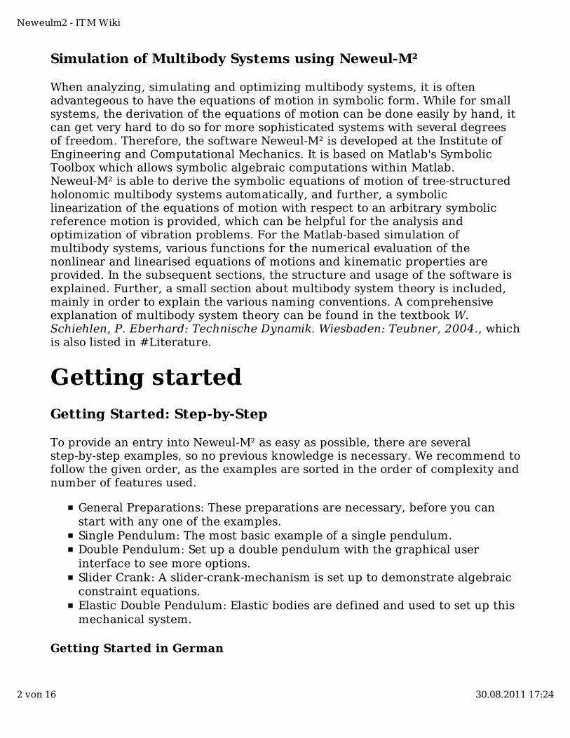
Simulation of Multibody Systems using Neweul-M²
When analyzing, simulating and optimizing multibody systems, it is oftenadvantegeous to have the equations of motion in symbolic form. While for smallsystems, the derivation of the equations of motion can be done easily by hand, itcan get very hard to do so for more sophisticated systems with several degreesof freedom. Therefore, the software Neweul-M² is developed at the Institute ofEngineering and Computational Mechanics. It is based on Matlab's SymbolicToolbox which allows symbolic algebraic computations within Matlab.Neweul-M² is able to derive the symbolic equations of motion of tree-structuredholonomic multibody systems automatically, and further, a symboliclinearization of the equations of motion with respect to an arbitrary symbolicreference motion is provided, which can be helpful for the analysis andoptimization of vibration problems. For the Matlab-based simulation ofmultibody systems, various functions for the numerical evaluation of thenonlinear and linearised equations of motions and kinematic properties areprovided. In the subsequent sections, the structure and usage of the software isexplained. Further, a small section about multibody system theory is included,mainly in order to explain the various naming conventions. A comprehensiveexplanation of multibody system theory can be found in the textbook W.Schiehlen, P. Eberhard: Technische Dynamik. Wiesbaden: Teubner, 2004., whichis also listed in #Literature.
Getting started
Getting Started: Step-by-Step
To provide an entry into Neweul-M² as easy as possible, there are severalstep-by-step examples, so no previous knowledge is necessary. We recommend tofollow the given order, as the examples are sorted in the order of complexity andnumber of features used.
General Preparations: These preparations are necessary, before you canstart with any one of the examples.Single Pendulum: The most basic example of a single pendulum.Double Pendulum: Set up a double pendulum with the graphical userinterface to see more options.Slider Crank: A slider-crank-mechanism is set up to demonstrate algebraicconstraint equations.Elastic Double Pendulum: Elastic bodies are defined and used to set up thismechanical system.
Getting Started in German
Neweulm2 - ITM Wiki
2 von 16 30.08.2011 17:24
Allgemeine Vorbereitungen: Vorbereitungen, die vor den Beispielennotwendig sind.Einfachpendel: Einfaches EinstiegsbeispielDoppelpendel: Doppelpendel, an dem mehr Optionen gezeigt werden.Schubkurbeltrieb: Ein Schubkurbeltrieb, um algebraischeNebenbedingungen zu erklären.Elastisches Doppelpendel: Definition von elastischen Körpern undEinbindung davon in ein Mehrkörpersystem.
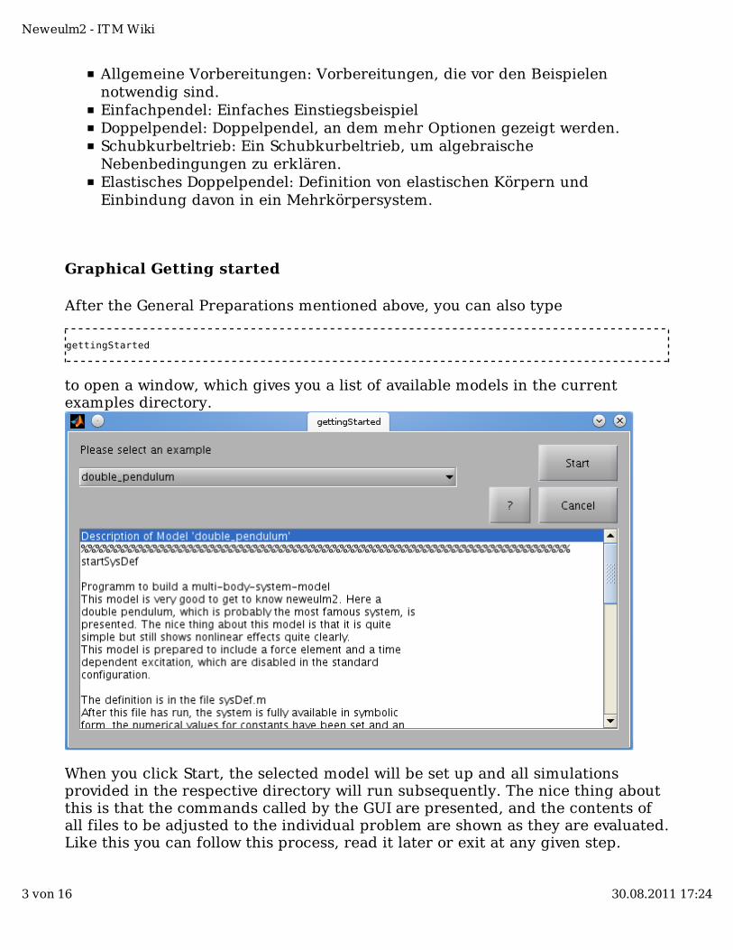
Graphical Getting started
After the General Preparations mentioned above, you can also type
gettingStarted
to open a window, which gives you a list of available models in the currentexamples directory.
When you click Start, the selected model will be set up and all simulationsprovided in the respective directory will run subsequently. The nice thing aboutthis is that the commands called by the GUI are presented, and the contents ofall files to be adjusted to the individual problem are shown as they are evaluated.Like this you can follow this process, read it later or exit at any given step.
Neweulm2 - ITM Wiki
3 von 16 30.08.2011 17:24
Cheat sheet
If you already know something about the possibilities of Neweul-M² and justneed a very short summary of the main commands and there option, you maywant to look at our cheat sheet (http://www.itm.uni-stuttgart.de/itmwiki/wikidata/cheatSheet.pdf) .
General information
Compatible Matlab versions
The software is currently being developed under Matlab R2007b and R2010b.The software has been tested under matlabR2006a, but there is one importantissue. When using Neweul-M² outside of the institute, the files have beenprecompiled and are thus unreadable. This precompilation is notdown-compatible. So when you want to use e.g. Matlab version R2006a, pleaseask your contact person at the ITM for a suitable version of the software.
If you are using a Matlab of Version R2007b+ and newer, the Symbolic MathToolbox is no longer using a Maple kernel. Instead MuPad is used for symboliccalculations. For such commands, wrapper functions have been introduced,called mapleSimplify and mapleSubs. Usually it is faster and provides moreoptions when Maple is called directly instead of using the built-in Matlabfunctions. In a recent update, these wrapper functions should be able todetermine the symbolic engine and use the correct commands. Before this itwas necessary to adjust both of these wrapper functions to use the appropriatecode. It is not so easy to determine, which way of calling is faster, because thespeed depends strongly on the size and type of expressions. Therefore the usercould try to use one of the other provided algorithms for special cases. Thesefunctions should be excluded from the precompilation and you can thereforeread and adjust them to your needs.
MuPad reserved some parameter names like beta or I for internal functions.Please be careful when moving models from one symbolic engine to another. Formore information see Restrictions for Names
Symbolic - Numeric - What?Neweul-M² calculates the equations of motion symbolically. This means it usesnames like m1 for the parameters and not numbers 5 [kg] to set up theequations. This has several advantages, allowing the user to read and understandthe expressions and allowing an explicit formulation. Also you can change valueswithout recalculating the equations of motion. As not everything can be done
Neweulm2 - ITM Wiki
4 von 16 30.08.2011 17:24
symbolically, the numbers come in at some point in the simulation. But alwayswhen you have two uses (symbolic and numeric) of the same things, there aresome problems. To keep these as small as possible the complete data is stored intwo ways simultaneously:
the symbolic expressions are stored in the structure sys, available in theworkspace.files containing source code, which will evaluate numerical values.
Even if you only want the files to calculate numerical values, it might be good tosave the system after modeling. When doing so in the menu of the GUI, it willsave the figure and the data structure containing the symbolic expressions. Theadvantage is that you can load the data structure, change something andrecreate the files. If you forgot to save before closing or the program crashed,you can still hope for the autosave. Every few minutes, your system is savedautomatically to examples/sandbox/autosave.mat. In this case you should make acopy of the autosave files, otherwise they might be overwritten, the next timeyou do anything in Neweul-M².
Using Neweul-M² at the ITMThe following part is dedicated to using the software package at the ITM,University of Stuttgart. Probably they are of no importance when using thesoftware somewhere else, but these explanations are available internally as awiki and externally as a pdf export of the very same text.
Ways to use Neweul-M²
There are two versions available, one running on the server and stored locally.Who should use which version?With both versions, you can model a system, run simulations and analysis. Pleaseanswer the following questions:
Do I want to write a new feature?Do I want to improve the current program?Do I want to work on a computer without connection to the ITM-Network?
If you answered at least one question with 'yes', then please get a local versionwith SVN. Otherwise please use the server-version.
Do NOT copy the files manually to get a local version!!!This will cause you to miss all updates from this day on. And if you changedsomething it is a hell of a job to insert these changes in the current version.
Neweulm2 - ITM Wiki
5 von 16 30.08.2011 17:24
Server version
For most users located at the ITM, the best way to call Neweul-M² is to use theserver version. If you already have a model or just don't need the examples allyou have to do is type
addpathNeweulm2
This is a file available in your search path, which will make sure all necessaryfiles are available. This basically is an abbreviation of the command
addpath(genpath('/home/itm/itmsw/neweulm2/currentVersion/neweulm2/'));
This makes all functions available for you. If you don't want to have to rememberthis, you can add this line to the file ~/matlab/startup.m which executes ateach start of Matlab.
If you are using the Matlab command restoredefaultpath, you will need tospecify the path again explicitly.
When using the server version you can store the model folders with your input orsimulation data and all the routines can stay on the server. Like this you will notbe able to change anything at the code, but can edit and create models in yourlocal folder. You can find this version at /home/itm/itmsw/neweulm2/currentVersion/ (Before renaming /home/itm/itmsw/symbs/symbsServer/). Thisfolder contains a complete set of all files. The best way to start is to copy theexamples folder to your account or a scratch partition on your PC. Then you canhave a look at prepared examples and adjust them to your needs. You can do thisby opening a shell, changing to the desired folder in your account and enter thefollowing command:
cp -r /home/itm/itmsw/neweulm2/currentVersion/examples/ .
By this you will get a few examples, both for input files and for the graphic userinterface (GUI). In the folder sandbox/ you will find a file called Readme.txtgiving you an explanation on how to get started. To start the GUI, please call thefile link_neweulm2.m in Matlab, which you find in the sandbox/ folder.
Local version
If you want to change the routines of Neweul-M² or extend the functionality, e.g.for your research paper, you need a local copy. For this please follow thefollowing steps:1.) Please contact your system administrator in order to get the necessary
Neweulm2 - ITM Wiki
6 von 16 30.08.2011 17:24
permissions.2.) Open a shell (also called Console) and change to the folder, where you wantNeweul-M² in and type the following command. This will create a new foldercalled "neweulm2_local" containing all files. Then you are ready to go. In thisnewly created folder you will find a file called "Readme.txt" containinginformation on how to start Neweul-M² from Matlab.
git clone [email protected]:neweulm2.git
If you are asked for a password of itmgit, probably something went wrong withstep one.
At the beginning of each modeling with commands it has to be ensured that theroutines of Neweul-M² are available by adding the necessary path. If youreceived a copy of Neweul-M² and did not change too much in the directorystructure, you can also use the file
addpathNeweulm2
This is usually located at examples/addpathNeweulm2 and should cover mostcases of where your neweulm2/ directory is located. Otherwise, please type helpaddpathNeweulm2 for information on how to specify the path manually.
An explanation on how to use GIT can be found here: Git - Distributed VersionControl. To use a GIT-command, open a shell and change to the directory, whereyour local copy is located. The most important command, which should be calledfrom time to time is
git pull
which will update your local copy with the files from the server. If you changedsome files, which were changed on the server as well, GIT will tell you that andask you to resolve these conflicts.
If you programmed some new functions or made other improvements you wantto share with the other users please contact Thomas Kurz.
Starting Matlab
Neweul-M² is running under Matlab. At the institute there are several versions ofMatlab available, which can be seen, when opening a Command Shell, typing'matlab' and hitting the [Tab] Key twice. The program should run withoutproblems in all versions starting with 'matlabR20', while there are some knownproblems in lower versions up to '7.2'. If unsure which version to use, just call
Neweulm2 - ITM Wiki
7 von 16 30.08.2011 17:24
matlab which usually opens the newest version.
Neweul-M² - neweulm2 - SYMBS -NEWEULThe multibody program described here, started under the name SYMBS. Afterit appeared to be quite promissing it has been renamed to Neweul-M². Thisname is meant to underline that this program is successor of the FORTRANCode called NEWEUL. Because of this, some misleading names may occur. TheM² is a tribute to its two used math programs MATLAB and Maple. As thename Neweul-M² contains non-standard characters its function call isneweulm2, which is also used for the wiki pages here.
For HTML pages: The sign ² has the ASCII-Code &# 178; without the space.For LaTeX documents: it is most convenient to add this line to the Masterdocument
\newcommand{\neweulm}{\mbox{Neweul-M$^2$}}
Then the correct name is achieved by typing \neweulm{} in the document,where the brackets {} are necessary to ensure the correct spacing.
Release notesSome information on important new features can be found here: neweulm2 -Release notes
At each version you will find a file, which is called VersionLogfile.txt orpreviously symbs_CVS_Logfile.txt, which contains a more detailed decription ofthe changes.
Available ModelsTo get started with the program there are some easy models available:
Double Pendulum (directory: double_pendulum)Slider Crank (directory: slider_crank)Elastic Pendulum (directory: elasticPendulum)Half-car model (directory: car_half)An inverse modeled slider crank (directory: slider_crank_inverse)
Neweulm2 - ITM Wiki
8 von 16 30.08.2011 17:24
An example to demonstrate different force elements (directory:testForceElements)
The first three models are very good to get to know the software. You canobserve which files are in use, how to define different modeling elements, howto set up equations and how to start simulations. The other three models have aslightly different aim and are not as clearly documented as the first three. Thehalf-car is a fairly realistic model especially containing state dependentparameters to model nonlinear springs. The inverse modeled slider crank hasthe main goal to investigate different modeling techniques for systems withconstraint equations on a model with distinct singular configurations. The lastmodel-directory offers different models to investigate the behavior of forceelements. All of these models are also used for automated testing, which shouldhelp to detect errors in the software.
When during a student research paper or some other non-confidential project amodel is created it will be put in the following folder
/home/itm/itmsw/neweulm2/models/
The goal of this is to make more complex models available for the rest of theusers. Also this is meant as a kind of knowledge base, e.g. if you want to knowhow to use flexible bodies, gradients or some other feature, you find someexamples there.
To upload a model into this folder, you should make sure that it is runningunder the current version. There is no guarantee that they are up to date, sosome adjustments may be necessary before they run properly. Please insert aREADME.txt in each model folder with a short description of the model, whichalso contains the name of the printed research paper. Depending on the size andmode of creation this folder should contain:
sysDef.msetUserVar.m (if numeric values were not set in sysDef.m)defineGraphics.mThe folder userFunctions/ with all necessary functions for time- and state-dependent parameters.Any file to run a simulation tested by you, e.g. runTimeInt.mOptionally a .mat and .fig file of the saved system. Please check the size ofit before copying it there and maybe remove all results from the structure.
It should not contain
Badly commented filesFiles which produce errors even under the then current version.
Neweulm2 - ITM Wiki
9 von 16 30.08.2011 17:24
Analysis results
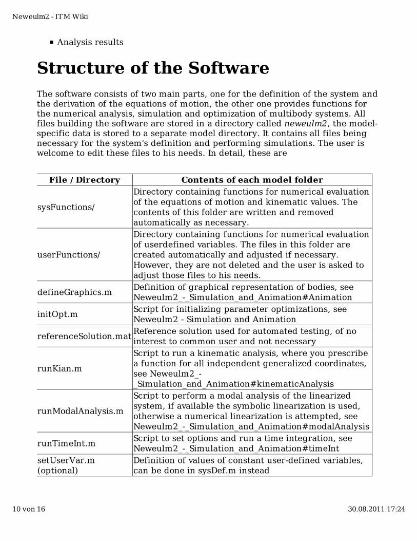
Structure of the SoftwareThe software consists of two main parts, one for the definition of the system andthe derivation of the equations of motion, the other one provides functions forthe numerical analysis, simulation and optimization of multibody systems. Allfiles building the software are stored in a directory called neweulm2, the model-specific data is stored to a separate model directory. It contains all files beingnecessary for the system's definition and performing simulations. The user iswelcome to edit these files to his needs. In detail, these are
File / Directory Contents of each model folder
sysFunctions/
Directory containing functions for numerical evaluationof the equations of motion and kinematic values. Thecontents of this folder are written and removedautomatically as necessary.
userFunctions/
Directory containing functions for numerical evaluationof userdefined variables. The files in this folder arecreated automatically and adjusted if necessary.However, they are not deleted and the user is asked toadjust those files to his needs.
defineGraphics.mDefinition of graphical representation of bodies, seeNeweulm2_-_Simulation_and_Animation#Animation
initOpt.mScript for initializing parameter optimizations, seeNeweulm2 - Simulation and Animation
referenceSolution.matReference solution used for automated testing, of nointerest to common user and not necessary
runKian.m
Script to run a kinematic analysis, where you prescribea function for all independent generalized coordinates,see Neweulm2_-_Simulation_and_Animation#kinematicAnalysis
runModalAnalysis.m
Script to perform a modal analysis of the linearizedsystem, if available the symbolic linearization is used,otherwise a numerical linearization is attempted, seeNeweulm2_-_Simulation_and_Animation#modalAnalysis
runTimeInt.mScript to set options and run a time integration, seeNeweulm2_-_Simulation_and_Animation#timeInt
setUserVar.m(optional)
Definition of values of constant user-defined variables,can be done in sysDef.m instead
Neweulm2 - ITM Wiki
10 von 16 30.08.2011 17:24
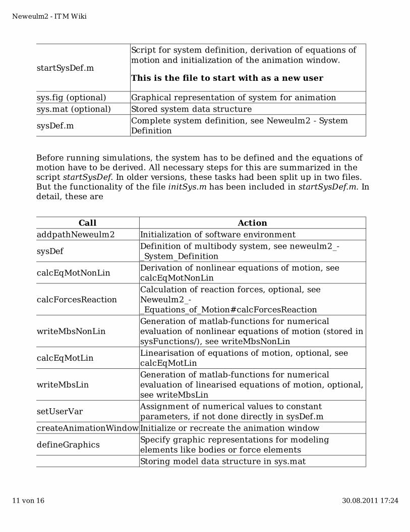
startSysDef.m
Script for system definition, derivation of equations ofmotion and initialization of the animation window.
This is the file to start with as a new user
sys.fig (optional) Graphical representation of system for animationsys.mat (optional) Stored system data structure
sysDef.mComplete system definition, see Neweulm2 - SystemDefinition
Before running simulations, the system has to be defined and the equations ofmotion have to be derived. All necessary steps for this are summarized in thescript startSysDef. In older versions, these tasks had been split up in two files.But the functionality of the file initSys.m has been included in startSysDef.m. Indetail, these are
Call ActionaddpathNeweulm2 Initialization of software environment
sysDefDefinition of multibody system, see neweulm2_-_System_Definition
calcEqMotNonLinDerivation of nonlinear equations of motion, seecalcEqMotNonLin
calcForcesReactionCalculation of reaction forces, optional, seeNeweulm2_-_Equations_of_Motion#calcForcesReaction
writeMbsNonLinGeneration of matlab-functions for numericalevaluation of nonlinear equations of motion (stored insysFunctions/), see writeMbsNonLin
calcEqMotLinLinearisation of equations of motion, optional, seecalcEqMotLin
writeMbsLinGeneration of matlab-functions for numericalevaluation of linearised equations of motion, optional,see writeMbsLin
setUserVarAssignment of numerical values to constantparameters, if not done directly in sysDef.m
createAnimationWindow Initialize or recreate the animation window
defineGraphicsSpecify graphic representations for modelingelements like bodies or force elementsStoring model data structure in sys.mat
Neweulm2 - ITM Wiki
11 von 16 30.08.2011 17:24
After these steps the system will be fully defined and ready for simulations.Neweul-M² offers many possibilities to perform simulations and analysis of thesystem, see neweulm2 - Simulation and Animation.
Graphical User Interface
A graphic user interface (GUI) can be found in neweulm2/gui/ and has beencreated with the Matlab GUI layout editor guide. It is created not independentlybut as a front-end to the existing version, which is controlled by input files.Therefore, it calls the same functions for the actual modeling and simulation.There are different ways to start it. If you've just started Matlab the best is tomove to the folder examples/sandbox/ and run the file link_neweulm2.m.This will then set up the Matlab path so the file neweulm2.m andstartneweulm2.m in the folder neweulm2/gui/ are found. There is a smalldifference between these two files.
When you call startneweulm2.m, the workspace is cleared, figures are closedand the gui is started. This means you are ready to go, but your workspace isempty. When running link_neweulm2.m also this startneweulm2 is called. Ifstill this is not convenient for you, you can call the functionwriteneweulm2link.m after starting the GUI. This will create a file also calledlink_neweulm2.m, but this time with the absolute path stored inside, thereforemaking it possible to start the GUI from any given folder. Many of the input filescan be created from the GUI under the menu entry Export System to ensurecompatibility in both ways.
When you call neweulm2 directly the workspace as well as all figures are keptand only the GUI is started. Therefore, this presents the easiest way to switchfrom input files to the GUI. You simply run the input files, type neweulm2 andthen you can work on the current model. Also, you can type Neweul-M²commands or close the GUI at any time and continue working solely withcommands. With the only exception that, if you select Exit from the File menu,then the workspace will be cleared. In order to keep the model you should selectClose Menu or click on the little cross in the upper right corner.
Another way of switching the way to control Neweul-M² is to save your model asa .mat file and load it in the other mode. Sometimes it happens that strangeerrors occur when some elements like bodies are deleted in the GUI. If that isthe case, simply open Export System from the File menu and create the Inputfiles. This will create one file containing all definitions which can be used toeasily rebuild your model from scratch.
HelpThere are a few possibilities on how to get help on neweulm2, before asking
Neweulm2 - ITM Wiki
12 von 16 30.08.2011 17:24
someone, see #See also.
ZB-149: This was the first documentation of Symbs and marks the firstappearance.Readme.txt: In each version of Symbs contains a Readme.txt whichexplains the most important things.VersionLogfile.txt or formerly symbs_CVS_Logfile.txt: This is a log-file ofall files that changed during the evolution of Symbs/Neweul-M². If you'renot sure which version you run, check this file.Online help in the GUI: In each window of the GUI you will find a buttonlabeled [?] which will display a help if there is one available. These helpmessages are stored in the folder neweulm2/gui/Definition/ in a file calledneweulm2HelpMsgs.m.This wiki: This is the most extensive ressource on Neweul-M². From time totime I export the contents of this wiki to a pdf-file, which can be foundunder
/home/itm/itmsw/neweulm2/currentVersion/NeweulM2_Manual.pdf
If you already know something about the possibilities of Neweul-M² and justneed a very short summary of the main commands and the their options,you may want to look at our cheat sheet (http://www.itm.uni-stuttgart.de/itmwiki/wikidata/cheatSheet.pdf) .
If you think there are some important things missing or could be explainedbetter in any of the still updated help channels, please help! Edit the entries inthis wiki, edit/change/create any help you think you can improve and send it tothe current supervisor of Neweul-M²!
There will be other users after you and probably they will encounter thesame problems if you don't fix them!
Function reference
Structure of the documentation
Experience showed that a wiki is a great vehicle to keep the documentation of asoftware project up to date. This bases on the fact that many people can updateand extend it. Still every single file, function and subfunction is to receive aheader containing information which can be accessed via Matlab's helpcommand or the F1 key. It is not helpful for anyone to store documentationredundantly, because then usually one source will be out of date.
Neweulm2 - ITM Wiki
13 von 16 30.08.2011 17:24
Contents of this wiki
A wiki provides an easy overview over available functions, the structure of thesoftware and comments on how to start. This makes it the place e.g. for thestep-by-step tutorials. In a wiki, pictures, formated text and formulae can beeasily displayed, which is very useful, e.g. for the detailed explanation of appliedforces. So the wiki shall provide the following contents:
overview over the software and implemented featuresstep-by-step introductioncurrent changes and new featuresreferences to how the theory works or where you can get furtherinformationdetailed explanations of topics too long or too complicated for the helpsection in a function
Contents of the function help header
As it is contained right inside the actual function, a short description of itspurpose and functionality have to be contained. This is also the easiest locationto keep information about in- and output arguments up to date. Therefore, thesethings together with all possible options are to be documented there. Eachfunction's help message shall provide the following contents:
Syntax of the function callwhat are available options and how to choose themwhat are the data types going in and coming out of the functionstandard values if you don't specify optionscontained subfunctions and links to related functionsgeneral information like the system data structure, file creation, ...
Overview over the wiki documentation
A more detailed description of the different functions can be found here:
neweulm2 - System Definitionneweulm2 - Equations of Motionneweulm2 - Simulation and Animationneweulm2 - Exporting
Or a neweulm2 - List of files is available to search in the other direction, by filename.
There is a list of Frequently Asked Questions neweulm2 - FAQ. However, theyare not intended to get into the software but to help when you started
Neweulm2 - ITM Wiki
14 von 16 30.08.2011 17:24
successfully and are now facing some problems.
Notes for programersIf you want to contribute to Neweul-M², please feel free to do so. On thefollowing page you can find a few hints on how you can make your program fitto all the rest. neweulm2 - Programming tips
See also
ITM Wiki
Explanation of the functions
Function reference: Search by topicneweulm2 - System Definitionneweulm2 - Equations of Motionneweulm2 - Simulation and Animationneweulm2 - Exporting
neweulm2 - List of files: Search by filename
Other topics
Neweulm2 - Getting Started: Step by step explanations for simple examples.neweulm2 - FAQ: Frequently asked questions and some tips that just don'tfit in other categories.Neweulm2 - Release notes: Short summary of every change.
ITM Server
PDF Export of these Wiki pages:/home/itm/itmsw/neweulm2/currentVersion/info/Neweulm2_Manual.pdf
STUD-344: Untersuchungen zur Auslegung und Realisierung einesParallelkinematik-Prüfstands, 2010./home/itm/institut/studdipl/STUD/STUD_344_FelixGeibel/stud_344.pdf
STUD-338: Erweiterung von Neweul-M² um die Berechnung vonReaktionskräften, 2010./home/itm/institut/studdipl/STUD/STUD_338_BernhardFeistle/stud_338.pdf
STUD-323: Programmvergleich für die Simulation elastischer
Neweulm2 - ITM Wiki
15 von 16 30.08.2011 17:24
Mehrkörpersysteme, 2010./home/itm/institut/studdipl/STUD/STUD_323_BernhardZeumer/stud_323.pdf
STUD-309: Kosimulation von Tankfahrzeugen mit Neweul-M² und Pasimodo,2009./home/itm/institut/studdipl/STUD/STUD_309_FrankSandner/stud_309.pdf
STUD-292: Implementierung flexibler Mehrkörpersysteme inMATLAB/SIMULINK auf Basis von Neweul-M², 2008./home/itm/institut/studdipl/STUD/STUD_292_MarkusBurkhardt/stud_292.pdf
DIPL-122: Entwicklung eines Optimierungsmoduls mit Sensitivitätsanalysefür die symbolische Mehrkörpersimulationsumgebung SYMBS, 2007./home/itm/institut/studdipl/DIPL/DIPL_122_ThomasKurz/dipl_122.pdf
STUD-263: Erstellung einer symbolischenMehrkörpersimulationsumgebung in MATLAB mit graphischerBenutzeroberfläche und verschiedenen Schnittstellen, 2007./home/itm/institut/studdipl/STUD/STUD_263_MarkusLutz/stud_263.pdf
ZB-149: SYMBS eine Matlab-Umgebung zur Simulation vonMehrkörpersystemen, 2007./home/itm/institut/studdipl/ZB/ZB_149_Henninger/symbs_doku.pdf
Literature
W. Schiehlen, P. Eberhard: Technische Dynamik. Wiesbaden: Teubner,2004.
Retrieved from "http://www.itm.uni-stuttgart.de/itmwiki/index.php/Neweulm2"
This page was last modified 11:15, 26 August 2011.
Neweulm2 - ITM Wiki
16 von 16 30.08.2011 17:24
Neweulm2 - Getting StartedPreparations
From ITM Wiki
If you are using the server version at the ITM, please enter the followingcommands in the console:
cp -r /home/itm/itmsw/neweulm2/currentVersion/examples/ $HOME/ cd $HOME/examples/ matlab &
This will copy the examples folder from the server to your home directory,change to this folder and start matlab. If you are using Neweul-M² outside of theITM or a local version, please start matlab and move to the directory where yourcopy of the software is stored and go into the directory called examples. Fromnow on, all commands should be entered directly in the Matlab commandwindow.
An initialization of the search path is necessary by typing:
addpathNeweulm2
This command usually finds all necessary files by itself. You will only get aresponse if there has been any problem. When setting up a model andperforming some simulations, the software has to store some files. Therefore itis very convenient to create separate folders for each model you want to keep. Ifyou only want to try some things, e.g. like the getting started examples, youcould use the sandbox folder instead. So if you want to continue with theGetting-Started, we recommend to change to the sandbox folder.
cd sandbox
The next time you want to use Neweul-M², you just have to change to the correctfolder (e.g. cd $HOME/examples/sandbox) again and start Matlab by yourselfand call addpathNeweulm2.
Here is a link to a list of all Getting Started Examples.
Retrieved from "http://www.itm.uni-stuttgart.de/itmwiki/index.php/Neweulm2_-_Getting_Started_Preparations"
Neweulm2 - Getting Started Preparations - ITM Wiki
1 von 2 01.09.2011 15:24

This page was last modified 10:57, 18 August 2011.
Neweulm2 - Getting Started Preparations - ITM Wiki
2 von 2 01.09.2011 15:24
Neweulm2 - Getting StartedSinglePendulum
From ITM Wiki
Contents
1 Single pendulum1.1 System definition1.2 Setting up the equations of motion1.3 Time integration1.4 Display and interpretation of results1.5 Additional information and help1.6 Commands learned in this example1.7 Links
Single pendulum
Please make sure that you performed the General Preparations before startingwith this example.
In the first example we will show you how to use the Matlab command window togenerate a pendulum model with a minimum number of parameters inNeweul-M². The commands can be typed directly within the command window ofmatlab so that we can get the desired results.
System definition
With the command 'newSys' you define a new multibody system.
newSys
The system, which shall be set up is shown in the following sketch
Neweulm2 - Getting Started SinglePendulum - ITM Wiki
1 von 7 01.09.2011 15:25
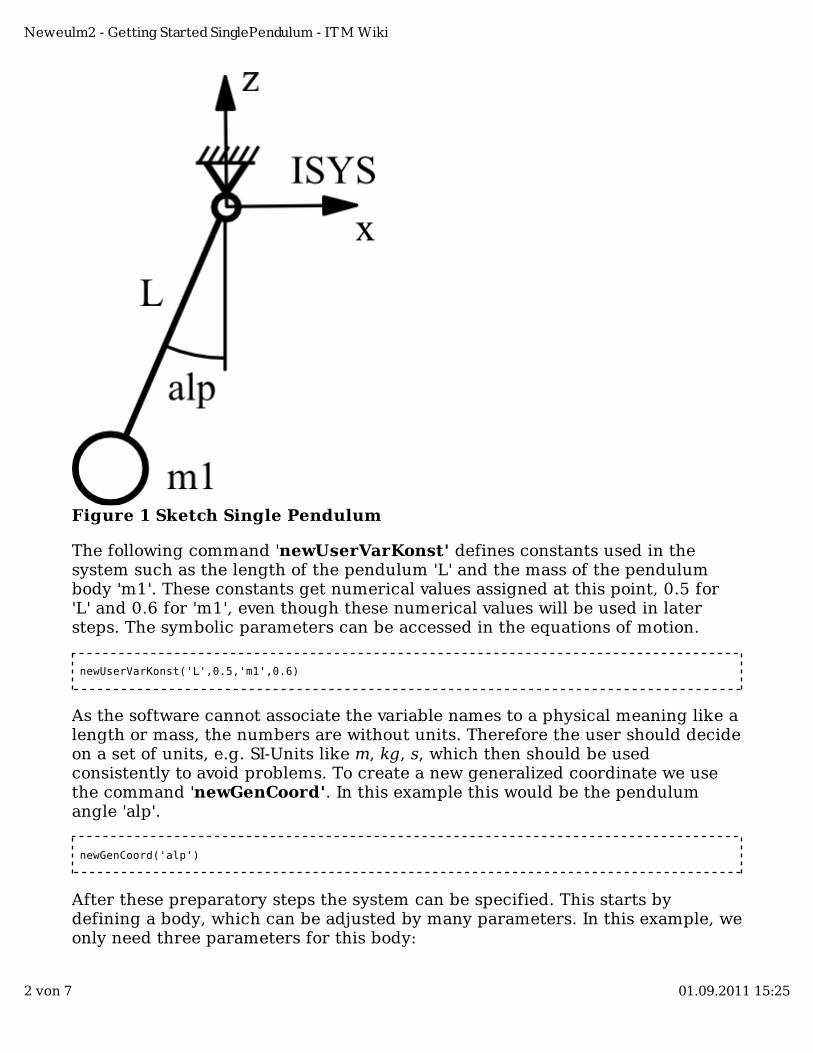
Figure 1 Sketch Single Pendulum
The following command 'newUserVarKonst' defines constants used in thesystem such as the length of the pendulum 'L' and the mass of the pendulumbody 'm1'. These constants get numerical values assigned at this point, 0.5 for'L' and 0.6 for 'm1', even though these numerical values will be used in latersteps. The symbolic parameters can be accessed in the equations of motion.
newUserVarKonst('L',0.5,'m1',0.6)
As the software cannot associate the variable names to a physical meaning like alength or mass, the numbers are without units. Therefore the user should decideon a set of units, e.g. SI-Units like m, kg, s, which then should be usedconsistently to avoid problems. To create a new generalized coordinate we usethe command 'newGenCoord'. In this example this would be the pendulumangle 'alp'.
newGenCoord('alp')
After these preparatory steps the system can be specified. This starts bydefining a body, which can be adjusted by many parameters. In this example, weonly need three parameters for this body:
Neweulm2 - Getting Started SinglePendulum - ITM Wiki
2 von 7 01.09.2011 15:25
the rotation around the y-axis relative to the inertial reference frame withthe generalized coordinate 'alp': 'RelRot','[0;alp;0]'
1.
the relative position of the center of gravity: 'CgPos','[0;0;-L]'2.the mass of the body: 'Mass','m1'.3.
newBody('RelRot','[0;alp;0]', 'CgPos','[0;0;-L]','Mass','m1')
Setting up the equations of motion
Now, as the single pendulum has already been defined completely, we cangenerate the nonlinear equations of motion using the command'calcEqMotNonLin'. The data is then stored in the global structure 'sys' andcan be accessed there.
calcEqMotNonLin
To write files for the numerical evaluation of these nonlinear equations ofmotion, the function 'writeMbsNonLin' is called.
writeMbsNonLin
To perform the simulation, numerical values are necessary. To show how thiscan be done at the current state, we change the pendulum length 'L' to 0.8 bythe command
sys.userVar.data.L = 0.8;
The last command was only used to demonstrate how to change a parametervalue. Of course, the value could be set correctly right at the definition of thevariable.
Time integration
Now we can perform the time integration. Therefore the initial condition 'y0 =0.5' has to be set. Now we can start the time integration with the command'timeInt(y0)'. All optional parameters are kept to their default values.
y0 = 0.5; result1 = timeInt(y0)
The results are stored in the data structure 'result1'. We can then start anothertime integration with other initial conditions such as 'y0_2 = 3.05'. The new
Neweulm2 - Getting Started SinglePendulum - ITM Wiki
3 von 7 01.09.2011 15:25
results are saved in the data structure 'result2'.
y0_2 = 3.05; result2 = timeInt(y0_2)
Display and interpretation of results
The results can be displayed using the following command:
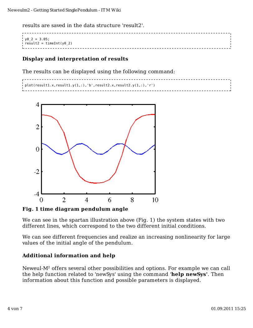
plot(result1.x,result1.y(1,:),'b',result2.x,result2.y(1,:),'r')
Fig. 1 time diagram pendulum angle
We can see in the spartan illustration above (Fig. 1) the system states with twodifferent lines, which correspond to the two different initial conditions.
We can see different frequencies and realize an increasing nonlinearity for largevalues of the initial angle of the pendulum.
Additional information and help
Neweul-M² offers several other possibilities and options. For example we can callthe help function related to 'newSys' using the command 'help newSys'. Theninformation about this function and possible parameters is displayed.
Neweulm2 - Getting Started SinglePendulum - ITM Wiki
4 von 7 01.09.2011 15:25
help newSys
By typing the command 'sys.eqm.qa' we can display the elements of the appliedforces. This is a cell array, referenced by curly braces {}, which contains onevector for each body. In our case, we have only one entry, which consists of thethree elements for the translation and three elements for the rotation, resultingin a 6x1 vector.
sys.eqm.qa{1}
If we were to start a time integration without specifying where to store theresults
timeInt(y0)
They are stored at the default location sys.results.timeInt. This is very useful, aswe could plot the generalized coordinate by typing
plotStandardResults
The advantage of this is that we don't have to worry about storage location ordimensions, as this is done automatically. If you stored the results at the defaultlocation, and you want to see an animation, you only need to type
createAnimationWindow
which will create an animation window and start the animation with thecommand
animTimeInt
In order to store this model, you only need to save the system data structure
save pendulum.mat sys
You can easily load the model, e.g. after a restart, by typing
load pendulum.mat
We are now at the end of the first demonstrative example. The following system
Neweulm2 - Getting Started SinglePendulum - ITM Wiki
5 von 7 01.09.2011 15:25
will be more complicated and we will use the graphical user interface (GUI). Thepurpose of the first example was to introduce you to how to use the commandwindow to build and simulate a simple model.
Commands learned in this example
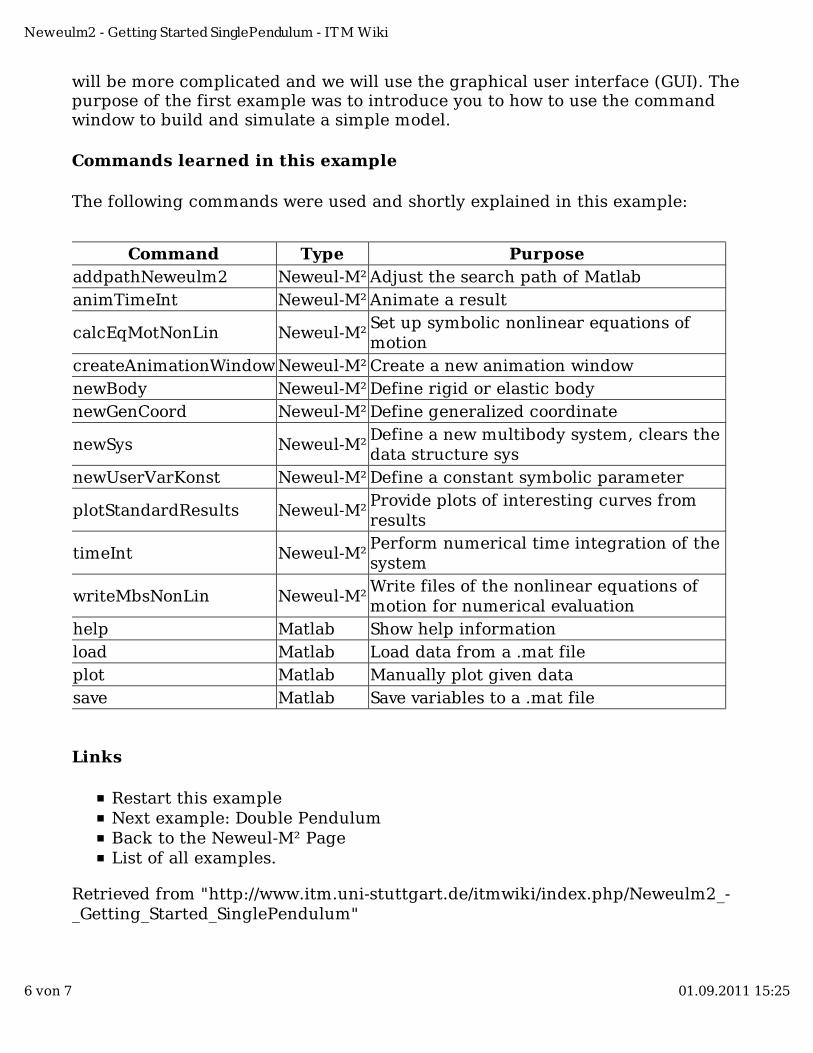
The following commands were used and shortly explained in this example:
Command Type PurposeaddpathNeweulm2 Neweul-M² Adjust the search path of MatlabanimTimeInt Neweul-M² Animate a result
calcEqMotNonLin Neweul-M²Set up symbolic nonlinear equations ofmotion
createAnimationWindow Neweul-M² Create a new animation windownewBody Neweul-M² Define rigid or elastic bodynewGenCoord Neweul-M² Define generalized coordinate
newSys Neweul-M²Define a new multibody system, clears thedata structure sys
newUserVarKonst Neweul-M² Define a constant symbolic parameter
plotStandardResults Neweul-M²Provide plots of interesting curves fromresults
timeInt Neweul-M²Perform numerical time integration of thesystem
writeMbsNonLin Neweul-M²Write files of the nonlinear equations ofmotion for numerical evaluation
help Matlab Show help informationload Matlab Load data from a .mat fileplot Matlab Manually plot given datasave Matlab Save variables to a .mat file
Links
Restart this exampleNext example: Double PendulumBack to the Neweul-M² PageList of all examples.
Retrieved from "http://www.itm.uni-stuttgart.de/itmwiki/index.php/Neweulm2_-_Getting_Started_SinglePendulum"
Neweulm2 - Getting Started SinglePendulum - ITM Wiki
6 von 7 01.09.2011 15:25

This page was last modified 11:33, 31 August 2011.
Neweulm2 - Getting Started SinglePendulum - ITM Wiki
7 von 7 01.09.2011 15:25
Neweulm2 - Getting StartedDoublePendulum
From ITM Wiki
Contents
1 Double pendulum1.1 System definition (GUI)1.2 Setting up the equations of motion (GUI)1.3 Time integration and plot of states1.4 Graphic objects for the animation1.5 Linearization of the equations of motion1.6 Saving1.7 Commands learned in this example1.8 Links
Double pendulum
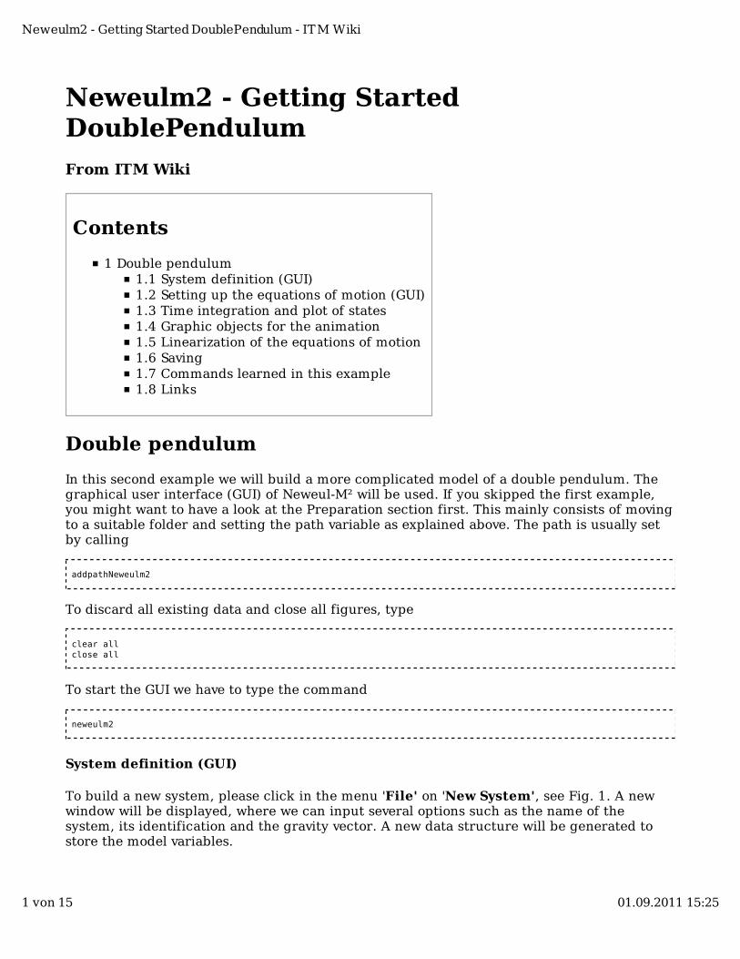
In this second example we will build a more complicated model of a double pendulum. Thegraphical user interface (GUI) of Neweul-M² will be used. If you skipped the first example,you might want to have a look at the Preparation section first. This mainly consists of movingto a suitable folder and setting the path variable as explained above. The path is usually setby calling
addpathNeweulm2
To discard all existing data and close all figures, type
clear all close all
To start the GUI we have to type the command
neweulm2
System definition (GUI)
To build a new system, please click in the menu 'File' on 'New System', see Fig. 1. A newwindow will be displayed, where we can input several options such as the name of thesystem, its identification and the gravity vector. A new data structure will be generated tostore the model variables.
Neweulm2 - Getting Started DoublePendulum - ITM Wiki
1 von 15 01.09.2011 15:25
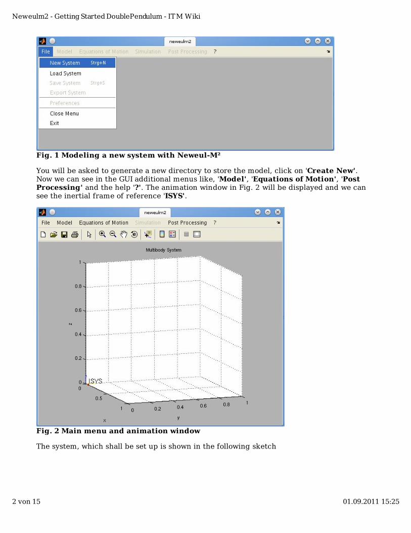
Fig. 1 Modeling a new system with Neweul-M²
You will be asked to generate a new directory to store the model, click on 'Create New'.Now we can see in the GUI additional menus like, 'Model', 'Equations of Motion', 'PostProcessing' and the help '?'. The animation window in Fig. 2 will be displayed and we cansee the inertial frame of reference 'ISYS'.
Fig. 2 Main menu and animation window
The system, which shall be set up is shown in the following sketch
Neweulm2 - Getting Started DoublePendulum - ITM Wiki
2 von 15 01.09.2011 15:25
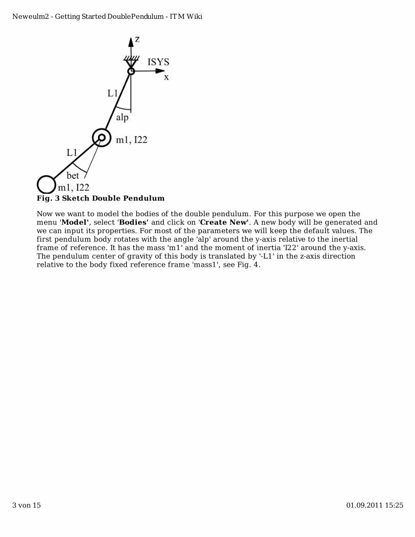
Fig. 3 Sketch Double Pendulum
Now we want to model the bodies of the double pendulum. For this purpose we open themenu 'Model', select 'Bodies' and click on 'Create New'. A new body will be generated andwe can input its properties. For most of the parameters we will keep the default values. Thefirst pendulum body rotates with the angle 'alp' around the y-axis relative to the inertialframe of reference. It has the mass 'm1' and the moment of inertia 'I22' around the y-axis.The pendulum center of gravity of this body is translated by '-L1' in the z-axis directionrelative to the body fixed reference frame 'mass1', see Fig. 4.
Neweulm2 - Getting Started DoublePendulum - ITM Wiki
3 von 15 01.09.2011 15:25
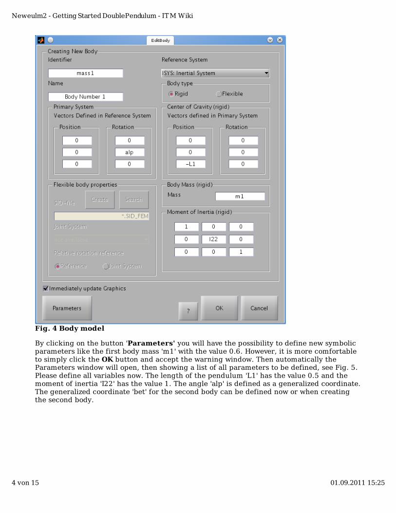
Fig. 4 Body model
By clicking on the button 'Parameters' you will have the possibility to define new symbolicparameters like the first body mass 'm1' with the value 0.6. However, it is more comfortableto simply click the OK button and accept the warning window. Then automatically theParameters window will open, then showing a list of all parameters to be defined, see Fig. 5.Please define all variables now. The length of the pendulum 'L1' has the value 0.5 and themoment of inertia 'I22' has the value 1. The angle 'alp' is defined as a generalized coordinate.The generalized coordinate 'bet' for the second body can be defined now or when creatingthe second body.
Neweulm2 - Getting Started DoublePendulum - ITM Wiki
4 von 15 01.09.2011 15:25
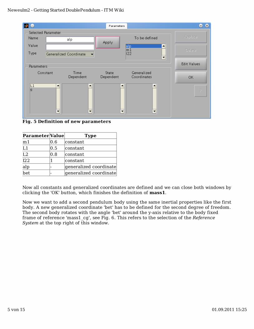
Fig. 5 Definition of new parameters
Parameter Value Typem1 0.6 constantL1 0.5 constantL2 0.8 constantI22 1 constantalp - generalized coordinatebet - generalized coordinate
Now all constants and generalized coordinates are defined and we can close both windows byclicking the 'OK' button, which finishes the definition of mass1.
Now we want to add a second pendulum body using the same inertial properties like the firstbody. A new generalized coordinate 'bet' has to be defined for the second degree of freedom.The second body rotates with the angle 'bet' around the y-axis relative to the body fixedframe of reference 'mass1_cg', see Fig. 6. This refers to the selection of the ReferenceSystem at the top right of this window.
Neweulm2 - Getting Started DoublePendulum - ITM Wiki
5 von 15 01.09.2011 15:25
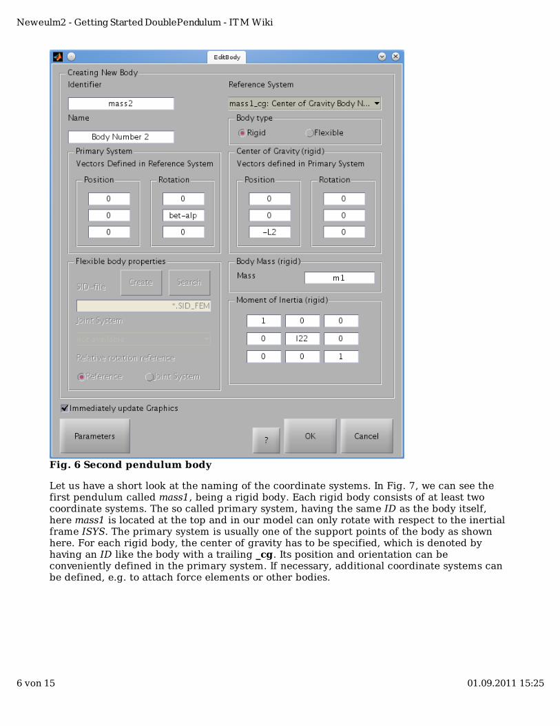
Fig. 6 Second pendulum body
Let us have a short look at the naming of the coordinate systems. In Fig. 7, we can see thefirst pendulum called mass1, being a rigid body. Each rigid body consists of at least twocoordinate systems. The so called primary system, having the same ID as the body itself,here mass1 is located at the top and in our model can only rotate with respect to the inertialframe ISYS. The primary system is usually one of the support points of the body as shownhere. For each rigid body, the center of gravity has to be specified, which is denoted byhaving an ID like the body with a trailing _cg. Its position and orientation can beconveniently defined in the primary system. If necessary, additional coordinate systems canbe defined, e.g. to attach force elements or other bodies.
Neweulm2 - Getting Started DoublePendulum - ITM Wiki
6 von 15 01.09.2011 15:25
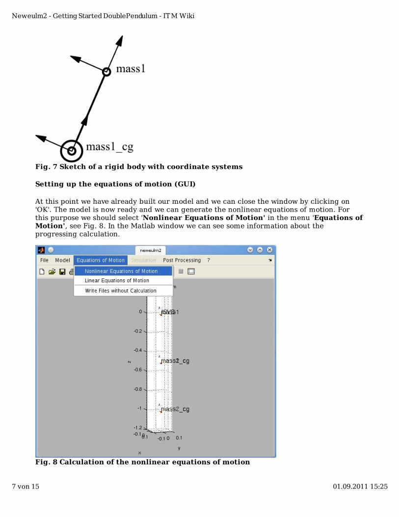
Fig. 7 Sketch of a rigid body with coordinate systems
Setting up the equations of motion (GUI)
At this point we have already built our model and we can close the window by clicking on'OK'. The model is now ready and we can generate the nonlinear equations of motion. Forthis purpose we should select 'Nonlinear Equations of Motion' in the menu 'Equations ofMotion', see Fig. 8. In the Matlab window we can see some information about theprogressing calculation.
Fig. 8 Calculation of the nonlinear equations of motion
Neweulm2 - Getting Started DoublePendulum - ITM Wiki
7 von 15 01.09.2011 15:25
Time integration and plot of states
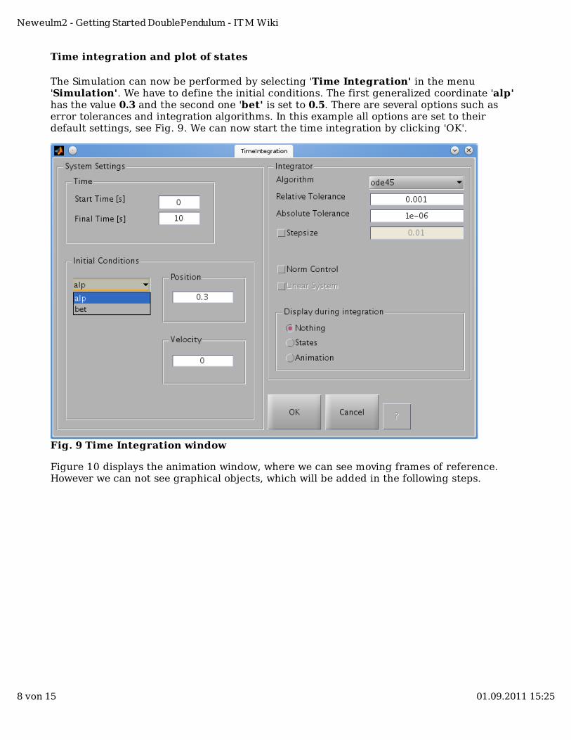
The Simulation can now be performed by selecting 'Time Integration' in the menu'Simulation'. We have to define the initial conditions. The first generalized coordinate 'alp'has the value 0.3 and the second one 'bet' is set to 0.5. There are several options such aserror tolerances and integration algorithms. In this example all options are set to theirdefault settings, see Fig. 9. We can now start the time integration by clicking 'OK'.
Fig. 9 Time Integration window
Figure 10 displays the animation window, where we can see moving frames of reference.However we can not see graphical objects, which will be added in the following steps.
Neweulm2 - Getting Started DoublePendulum - ITM Wiki
8 von 15 01.09.2011 15:25
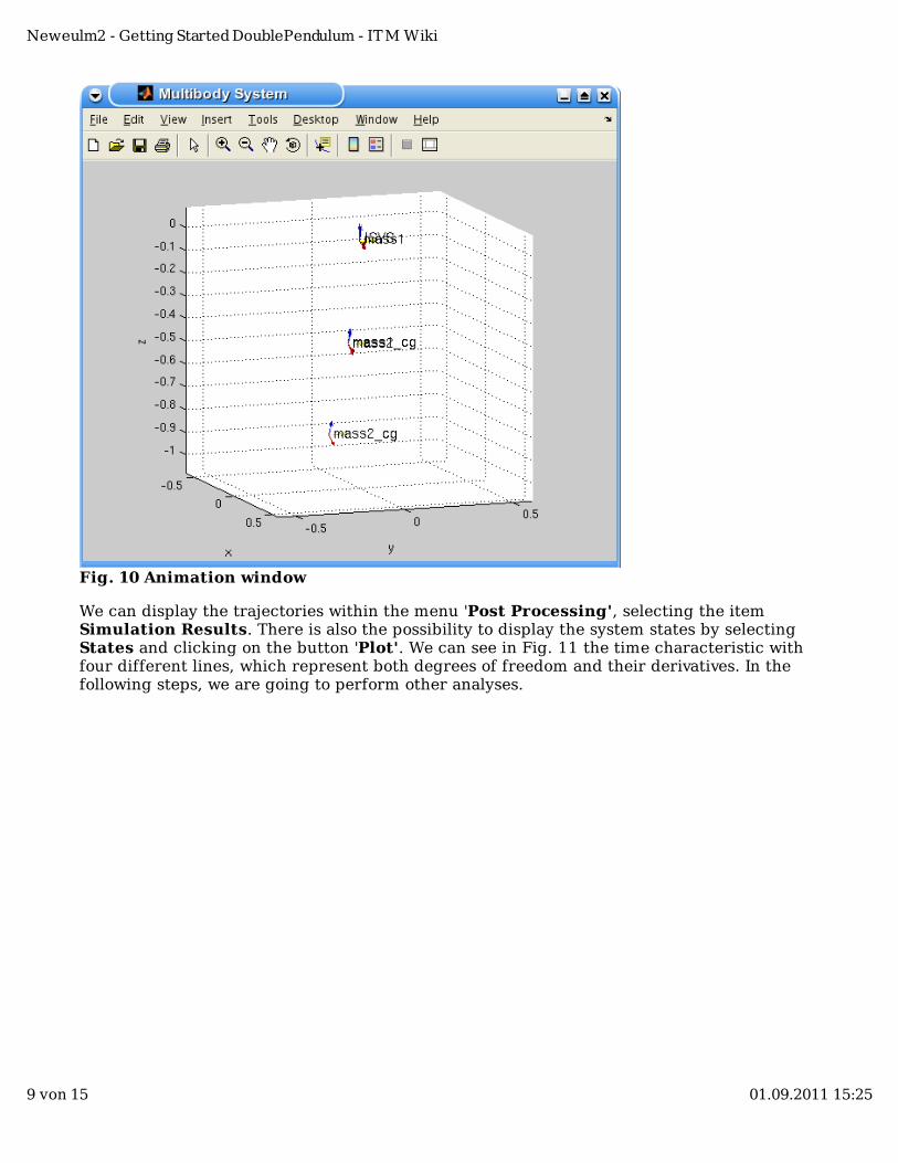
Fig. 10 Animation window
We can display the trajectories within the menu 'Post Processing', selecting the itemSimulation Results. There is also the possibility to display the system states by selectingStates and clicking on the button 'Plot'. We can see in Fig. 11 the time characteristic withfour different lines, which represent both degrees of freedom and their derivatives. In thefollowing steps, we are going to perform other analyses.
Neweulm2 - Getting Started DoublePendulum - ITM Wiki
9 von 15 01.09.2011 15:25
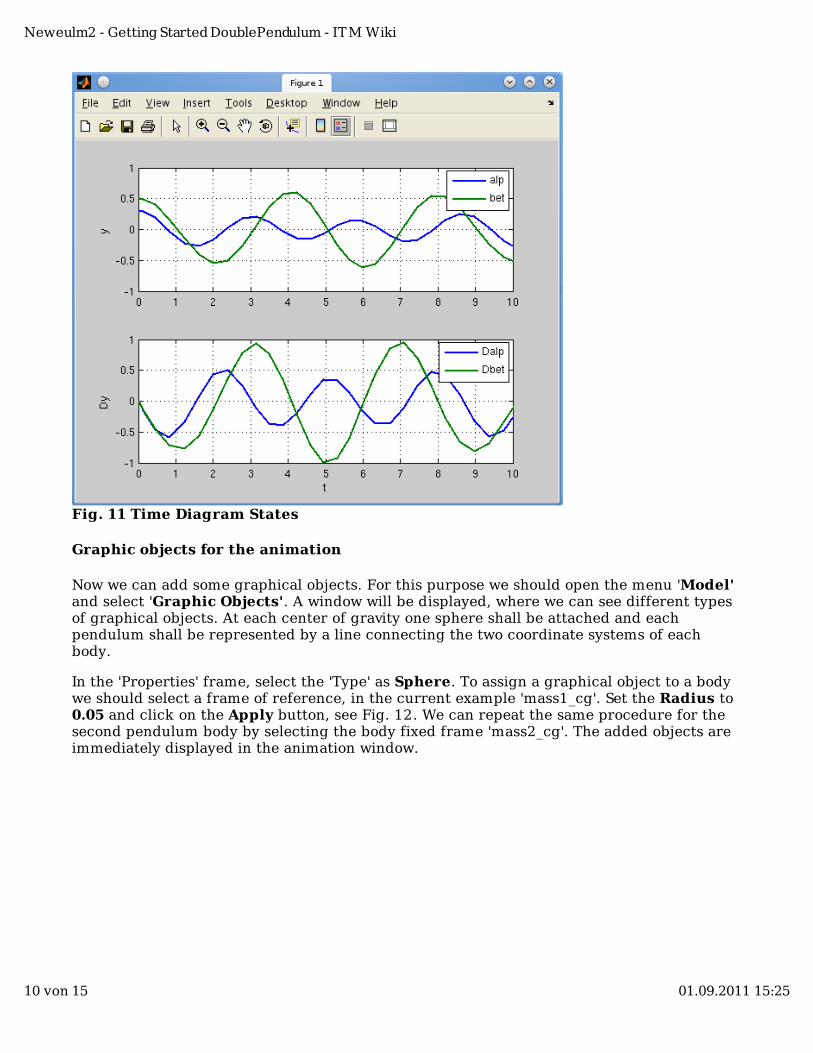
Fig. 11 Time Diagram States
Graphic objects for the animation
Now we can add some graphical objects. For this purpose we should open the menu 'Model'and select 'Graphic Objects'. A window will be displayed, where we can see different typesof graphical objects. At each center of gravity one sphere shall be attached and eachpendulum shall be represented by a line connecting the two coordinate systems of eachbody.
In the 'Properties' frame, select the 'Type' as Sphere. To assign a graphical object to a bodywe should select a frame of reference, in the current example 'mass1_cg'. Set the Radius to0.05 and click on the Apply button, see Fig. 12. We can repeat the same procedure for thesecond pendulum body by selecting the body fixed frame 'mass2_cg'. The added objects areimmediately displayed in the animation window.
Neweulm2 - Getting Started DoublePendulum - ITM Wiki
10 von 15 01.09.2011 15:25
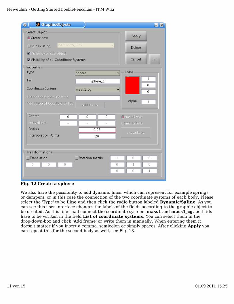
Fig. 12 Create a sphere
We also have the possibility to add dynamic lines, which can represent for example springsor dampers, or in this case the connection of the two coordinate systems of each body. Pleaseselect the 'Type' to be Line and then click the radio button labeled Dynamic/Spline. As youcan see this user interface changes the labels of the fields according to the graphic object tobe created. As this line shall connect the coordinate systems mass1 and mass1_cg, both idshave to be written in the field List of coordinate systems. You can select them in thedrop-down-box and click 'Add frame' or write them in manually. When entering them itdoesn't matter if you insert a comma, semicolon or simply spaces. After clicking Apply youcan repeat this for the second body as well, see Fig. 13.
Neweulm2 - Getting Started DoublePendulum - ITM Wiki
11 von 15 01.09.2011 15:25
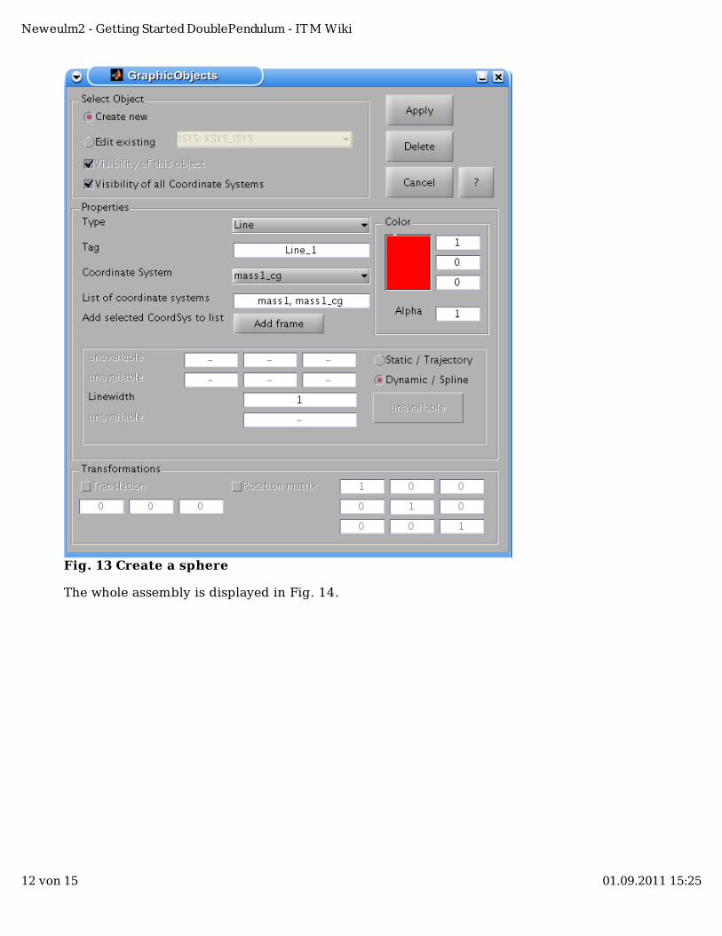
Fig. 13 Create a sphere
The whole assembly is displayed in Fig. 14.
Neweulm2 - Getting Started DoublePendulum - ITM Wiki
12 von 15 01.09.2011 15:25
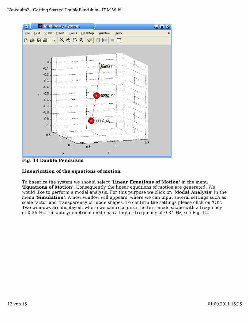
Fig. 14 Double Pendulum
Linearization of the equations of motion
To linearize the system we should select 'Linear Equations of Motion' in the menu'Equations of Motion'. Consequently the linear equations of motion are generated. Wewould like to perform a modal analysis. For this purpose we click on 'Modal Analysis' in themenu 'Simulation'. A new window will appears, where we can input several settings such asscale factor and transparency of mode shapes. To confirm the settings please click on 'OK'.Two windows are displayed, where we can recognize the first mode shape with a frequencyof 0.25 Hz, the antisymmetrical mode has a higher frequency of 0.34 Hz, see Fig. 15.
Neweulm2 - Getting Started DoublePendulum - ITM Wiki
13 von 15 01.09.2011 15:25
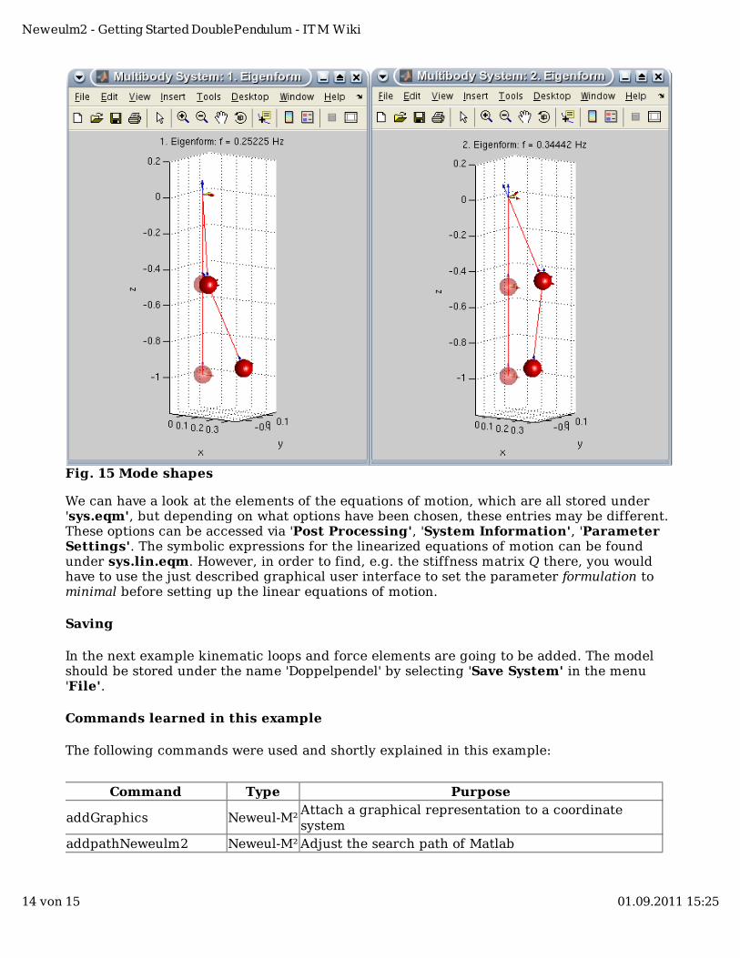
Fig. 15 Mode shapes
We can have a look at the elements of the equations of motion, which are all stored under'sys.eqm', but depending on what options have been chosen, these entries may be different.These options can be accessed via 'Post Processing', 'System Information', 'ParameterSettings'. The symbolic expressions for the linearized equations of motion can be foundunder sys.lin.eqm. However, in order to find, e.g. the stiffness matrix Q there, you wouldhave to use the just described graphical user interface to set the parameter formulation tominimal before setting up the linear equations of motion.
Saving
In the next example kinematic loops and force elements are going to be added. The modelshould be stored under the name 'Doppelpendel' by selecting 'Save System' in the menu'File'.
Commands learned in this example
The following commands were used and shortly explained in this example:
Command Type Purpose
addGraphics Neweul-M²Attach a graphical representation to a coordinatesystem
addpathNeweulm2 Neweul-M² Adjust the search path of Matlab
Neweulm2 - Getting Started DoublePendulum - ITM Wiki
14 von 15 01.09.2011 15:25
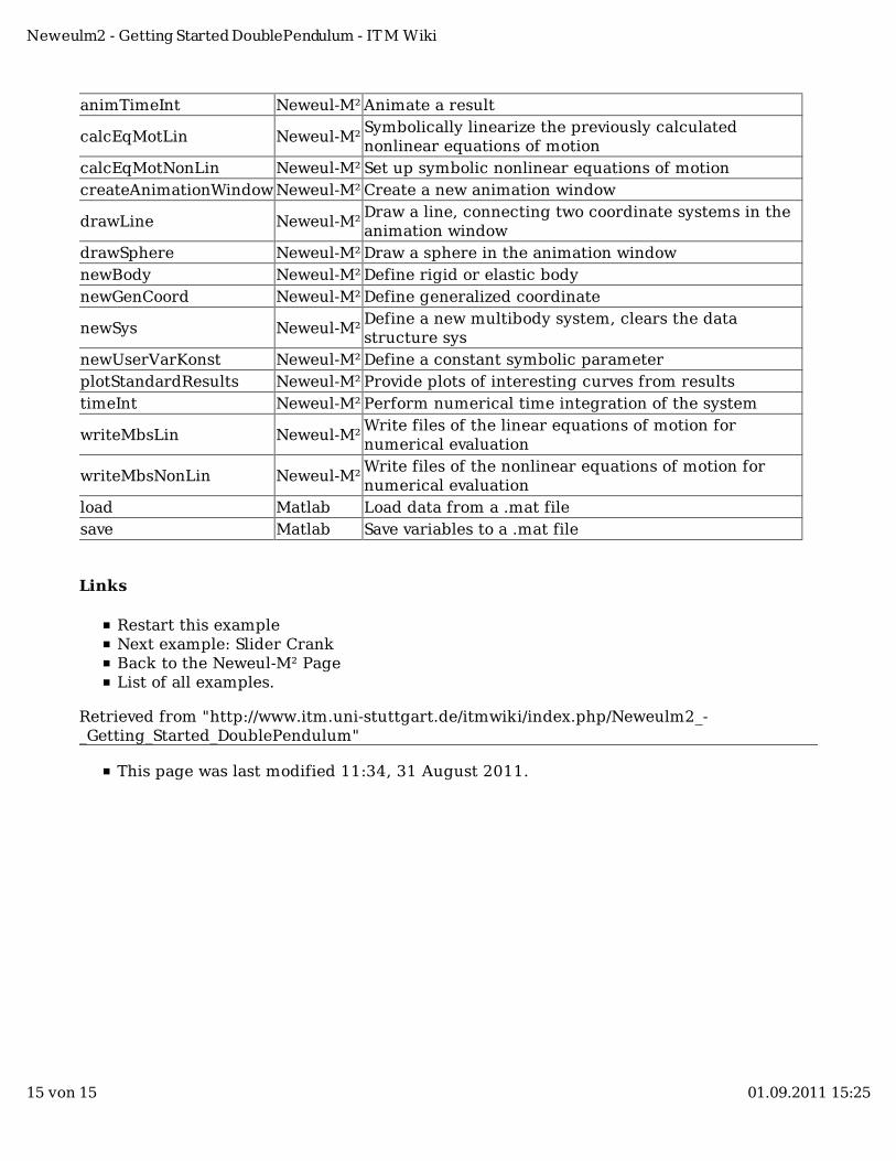
animTimeInt Neweul-M² Animate a result
calcEqMotLin Neweul-M²Symbolically linearize the previously calculatednonlinear equations of motion
calcEqMotNonLin Neweul-M² Set up symbolic nonlinear equations of motioncreateAnimationWindow Neweul-M² Create a new animation window
drawLine Neweul-M²Draw a line, connecting two coordinate systems in theanimation window
drawSphere Neweul-M² Draw a sphere in the animation windownewBody Neweul-M² Define rigid or elastic bodynewGenCoord Neweul-M² Define generalized coordinate
newSys Neweul-M²Define a new multibody system, clears the datastructure sys
newUserVarKonst Neweul-M² Define a constant symbolic parameterplotStandardResults Neweul-M² Provide plots of interesting curves from resultstimeInt Neweul-M² Perform numerical time integration of the system
writeMbsLin Neweul-M²Write files of the linear equations of motion fornumerical evaluation
writeMbsNonLin Neweul-M²Write files of the nonlinear equations of motion fornumerical evaluation
load Matlab Load data from a .mat filesave Matlab Save variables to a .mat file
Links
Restart this exampleNext example: Slider CrankBack to the Neweul-M² PageList of all examples.
Retrieved from "http://www.itm.uni-stuttgart.de/itmwiki/index.php/Neweulm2_-_Getting_Started_DoublePendulum"
This page was last modified 11:34, 31 August 2011.
Neweulm2 - Getting Started DoublePendulum - ITM Wiki
15 von 15 01.09.2011 15:25
Neweulm2 - Getting StartedSliderCrank
From ITM Wiki
Contents
1 Slider crank1.1 Load system1.2 System definition: force element, loop1.3 Time integration with kinematic loop1.4 Static Equilibrium1.5 Commands learned in this example1.6 Links
Slider crank
In this third example we are going to add a kinematic loop to the double pendulumabove. This means that the ordinary differential equations of motion will bechanged to algebraic differential equations. We will show you also how to add aforce element and how to calculate the static equilibrium. If you skipped theprevious example, you might want to have a look at the Preparation section first.This mainly consists of moving to a suitable folder and setting the path variable asexplained above.
Load system
For this purpose let’s call the GUI and from the menu 'File' select 'Load System'.The previous example (double pendulum) should be opened.
System definition: force element, loop
To add a force element we should select from the menu 'Model' the entry 'ForceElements', see Fig. 1.
Neweulm2 - Getting Started SliderCrank - ITM Wiki
1 von 9 01.09.2011 15:26
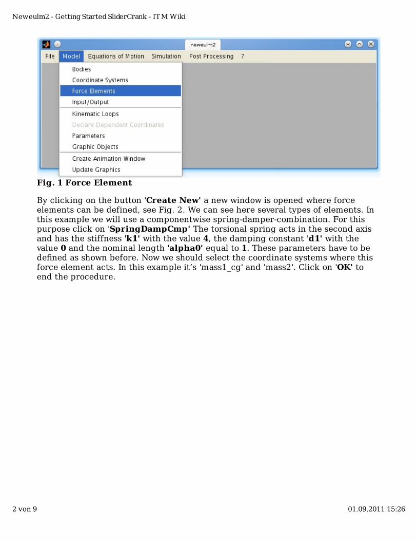
Fig. 1 Force Element
By clicking on the button 'Create New' a new window is opened where forceelements can be defined, see Fig. 2. We can see here several types of elements. Inthis example we will use a componentwise spring-damper-combination. For thispurpose click on 'SpringDampCmp' The torsional spring acts in the second axisand has the stiffness 'k1' with the value 4, the damping constant 'd1' with thevalue 0 and the nominal length 'alpha0' equal to 1. These parameters have to bedefined as shown before. Now we should select the coordinate systems where thisforce element acts. In this example it’s 'mass1_cg' and 'mass2'. Click on 'OK' toend the procedure.
Neweulm2 - Getting Started SliderCrank - ITM Wiki
2 von 9 01.09.2011 15:26
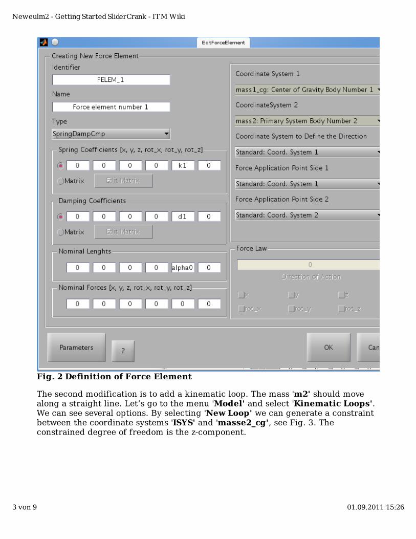
Fig. 2 Definition of Force Element
The second modification is to add a kinematic loop. The mass 'm2' should movealong a straight line. Let’s go to the menu 'Model' and select 'Kinematic Loops'.We can see several options. By selecting 'New Loop' we can generate a constraintbetween the coordinate systems 'ISYS' and 'masse2_cg', see Fig. 3. Theconstrained degree of freedom is the z-component.
Neweulm2 - Getting Started SliderCrank - ITM Wiki
3 von 9 01.09.2011 15:26
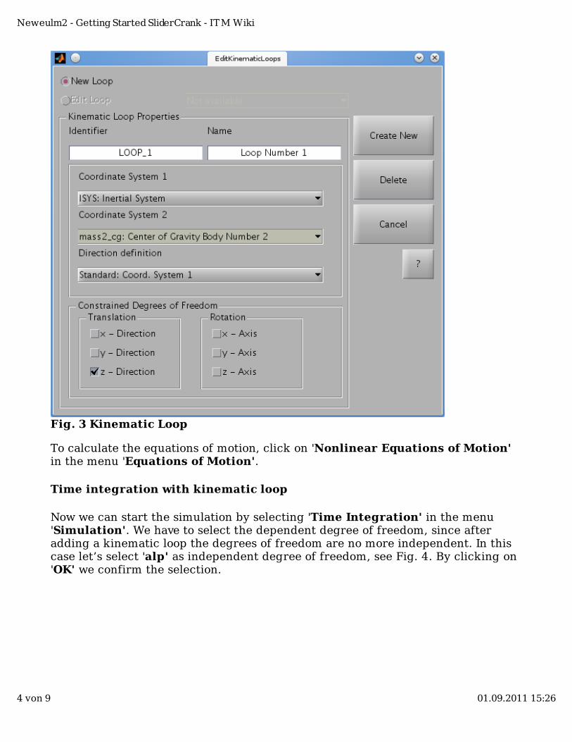
Fig. 3 Kinematic Loop
To calculate the equations of motion, click on 'Nonlinear Equations of Motion'in the menu 'Equations of Motion'.
Time integration with kinematic loop
Now we can start the simulation by selecting 'Time Integration' in the menu'Simulation'. We have to select the dependent degree of freedom, since afteradding a kinematic loop the degrees of freedom are no more independent. In thiscase let’s select 'alp' as independent degree of freedom, see Fig. 4. By clicking on'OK' we confirm the selection.
Neweulm2 - Getting Started SliderCrank - ITM Wiki
4 von 9 01.09.2011 15:26
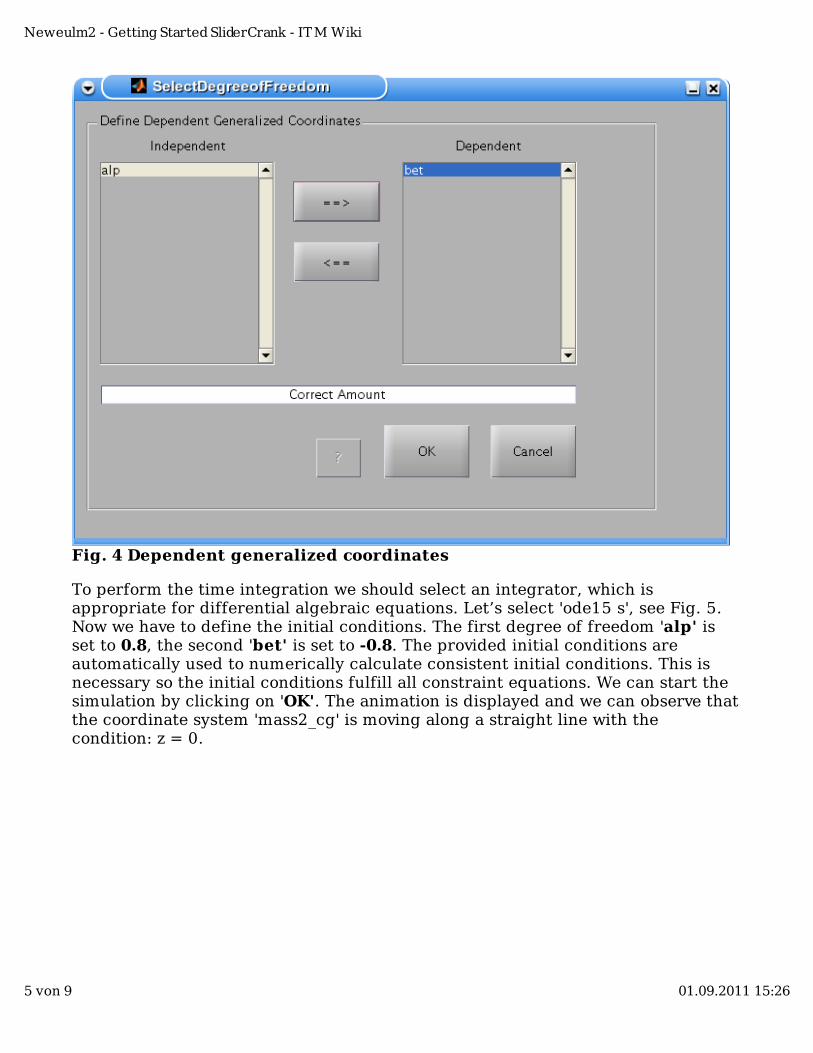
Fig. 4 Dependent generalized coordinates
To perform the time integration we should select an integrator, which isappropriate for differential algebraic equations. Let’s select 'ode15 s', see Fig. 5.Now we have to define the initial conditions. The first degree of freedom 'alp' isset to 0.8, the second 'bet' is set to -0.8. The provided initial conditions areautomatically used to numerically calculate consistent initial conditions. This isnecessary so the initial conditions fulfill all constraint equations. We can start thesimulation by clicking on 'OK'. The animation is displayed and we can observe thatthe coordinate system 'mass2_cg' is moving along a straight line with thecondition: z = 0.
Neweulm2 - Getting Started SliderCrank - ITM Wiki
5 von 9 01.09.2011 15:26
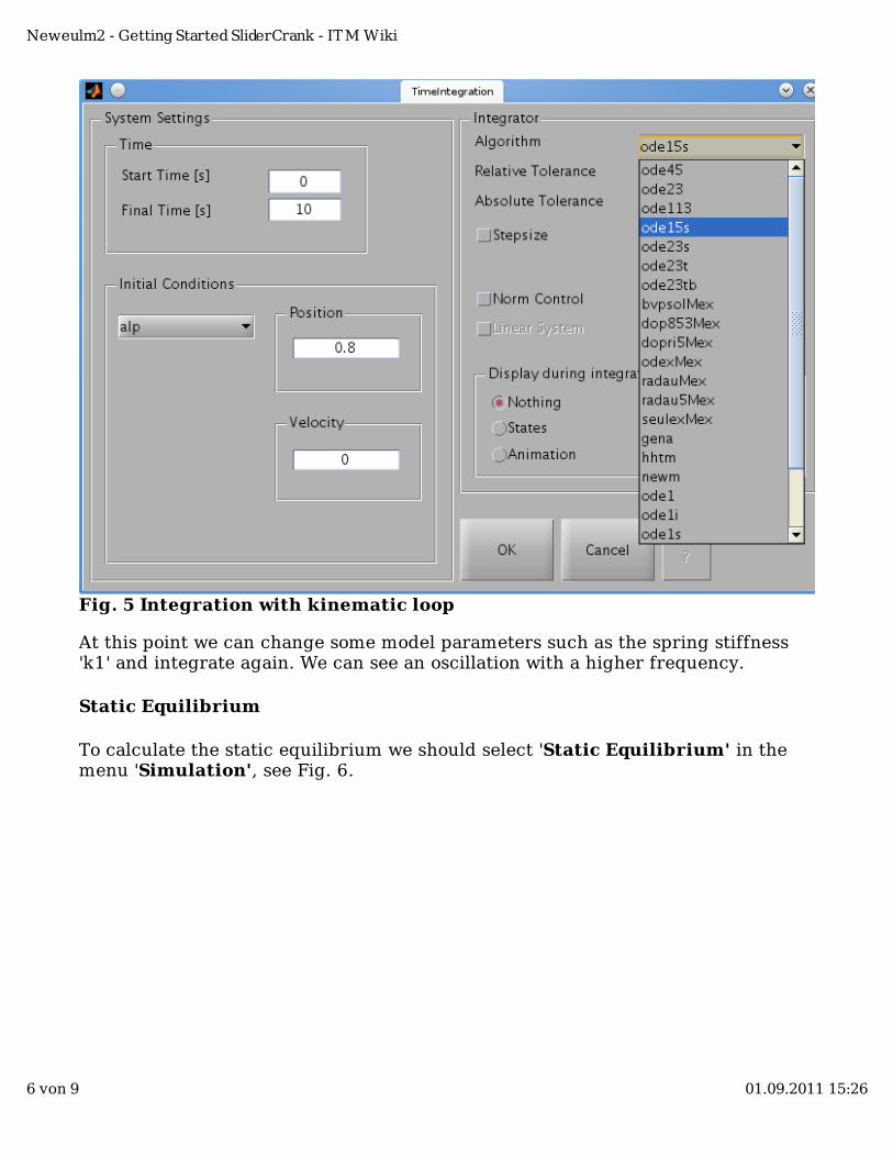
Fig. 5 Integration with kinematic loop
At this point we can change some model parameters such as the spring stiffness'k1' and integrate again. We can see an oscillation with a higher frequency.
Static Equilibrium
To calculate the static equilibrium we should select 'Static Equilibrium' in themenu 'Simulation', see Fig. 6.
Neweulm2 - Getting Started SliderCrank - ITM Wiki
6 von 9 01.09.2011 15:26

Fig. 6 Static Equilibrium
To perform the calculation we have to define a start value for the degree offreedom 'alp', see Fig. 7. The initial value should be near to the static equilibrium,so that the calculation does not require a high numerical expense.
Fig. 7 Start value for static equilibrium
By clicking on 'Static Equilibrium' the static equilibrium is calculated. Thegraphics is updated automatically or when changing a value.
Neweulm2 - Getting Started SliderCrank - ITM Wiki
7 von 9 01.09.2011 15:26
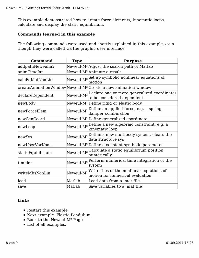
This example demonstrated how to create force elements, kinematic loops,calculate and display the static equilibrium.
Commands learned in this example
The following commands were used and shortly explained in this example, eventhough they were called via the graphic user interface:
Command Type PurposeaddpathNeweulm2 Neweul-M² Adjust the search path of MatlabanimTimeInt Neweul-M² Animate a result
calcEqMotNonLin Neweul-M²Set up symbolic nonlinear equations ofmotion
createAnimationWindow Neweul-M² Create a new animation window
declareDependent Neweul-M²Declare one or more generalized coordinatesto be considered dependent
newBody Neweul-M² Define rigid or elastic body
newForceElem Neweul-M²Define an applied force, e.g. a spring-damper combination
newGenCoord Neweul-M² Define generalized coordinate
newLoop Neweul-M²Define a new algebraic constraint, e.g. akinematic loop
newSys Neweul-M²Define a new multibody system, clears thedata structure sys
newUserVarKonst Neweul-M² Define a constant symbolic parameter
staticEquilibrium Neweul-M²Calculate a static equilibrium positionnumerically
timeInt Neweul-M²Perform numerical time integration of thesystem
writeMbsNonLin Neweul-M²Write files of the nonlinear equations ofmotion for numerical evaluation
load Matlab Load data from a .mat filesave Matlab Save variables to a .mat file
Links
Restart this exampleNext example: Elastic PendulumBack to the Neweul-M² PageList of all examples.
Neweulm2 - Getting Started SliderCrank - ITM Wiki
8 von 9 01.09.2011 15:26

Retrieved from "http://www.itm.uni-stuttgart.de/itmwiki/index.php/Neweulm2_-_Getting_Started_SliderCrank"
This page was last modified 11:34, 31 August 2011.
Neweulm2 - Getting Started SliderCrank - ITM Wiki
9 von 9 01.09.2011 15:26
Neweulm2 - Getting Started ElasticDoublePendulum
From ITM Wiki
Contents
1 Double pendulum with flexible bodies1.1 System definition (GUI)1.2 Setting up the equations of motion (GUI)1.3 Time integration and plot of states1.4 Analyzing the results
1.4.1 Commands learned in this example1.5 Links
Double pendulum with flexible bodies
In this example we build a double pendulum made up of two flexible beams, which will be animated by a shock. Therefore we use thegraphical user interface (GUI) of Neweul-M² again. The first step is to start Matlab again. If you skipped the first example, set the pathvariable as explained in the General Preparations, as a default:
addpathNeweulm2
To start the GUI we have to type the command
neweulm2
System definition (GUI)
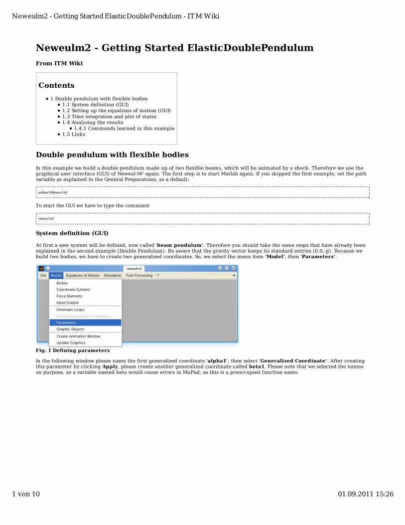
At first a new system will be defined, now called 'beam pendulum'. Therefore you should take the same steps that have already beenexplained in the second example (Double Pendulum). Be aware that the gravity vector keeps its standard entries (0,0,-g). Because webuild two bodies, we have to create two generalized coordinates. So, we select the menu item 'Model', then 'Parameters'.
Fig. 1 Defining parameters
In the following window please name the first generalized coordinate 'alpha1', then select 'Generalized Coordinate'. After creatingthis parameter by clicking Apply, please create another generalized coordinate called beta1. Please note that we selected the nameson purpose, as a variable named beta would cause errors in MuPad, as this is a preoccupied function name.
Neweulm2 - Getting Started ElasticDoublePendulum - ITM Wiki
1 von 10 01.09.2011 15:26
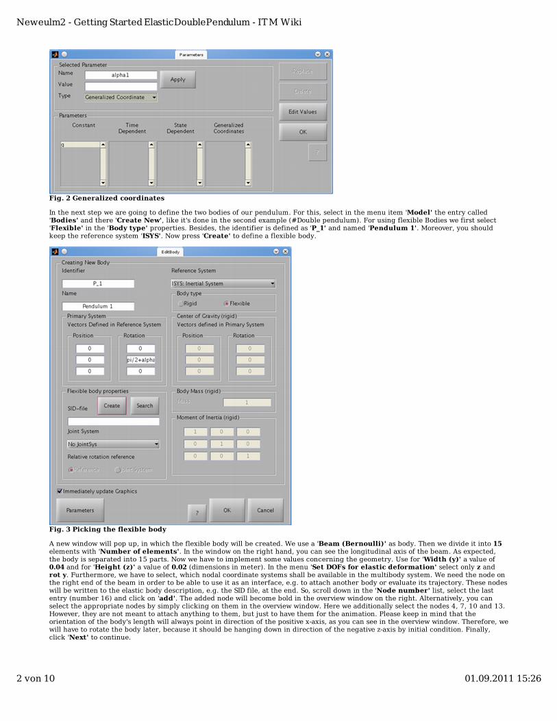
Fig. 2 Generalized coordinates
In the next step we are going to define the two bodies of our pendulum. For this, select in the menu item 'Model' the entry called'Bodies' and there 'Create New', like it's done in the second example (#Double pendulum). For using flexible Bodies we first select'Flexible' in the 'Body type' properties. Besides, the identifier is defined as 'P_1' and named 'Pendulum 1'. Moreover, you shouldkeep the reference system 'ISYS'. Now press 'Create' to define a flexible body.
Fig. 3 Picking the flexible body
A new window will pop up, in which the flexible body will be created. We use a 'Beam (Bernoulli)' as body. Then we divide it into 15elements with 'Number of elements'. In the window on the right hand, you can see the longitudinal axis of the beam. As expected,the body is separated into 15 parts. Now we have to implement some values concerning the geometry. Use for 'Width (y)' a value of0.04 and for 'Height (z)' a value of 0.02 (dimensions in meter). In the menu 'Set DOFs for elastic deformation' select only z androt y. Furthermore, we have to select, which nodal coordinate systems shall be available in the multibody system. We need the node onthe right end of the beam in order to be able to use it as an interface, e.g. to attach another body or evaluate its trajectory. These nodeswill be written to the elastic body description, e.g. the SID file, at the end. So, scroll down in the 'Node number' list, select the lastentry (number 16) and click on 'add'. The added node will become bold in the overview window on the right. Alternatively, you canselect the appropriate nodes by simply clicking on them in the overview window. Here we additionally select the nodes 4, 7, 10 and 13.However, they are not meant to attach anything to them, but just to have them for the animation. Please keep in mind that theorientation of the body's length will always point in direction of the positive x-axis, as you can see in the overview window. Therefore, wewill have to rotate the body later, because it should be hanging down in direction of the negative z-axis by initial condition. Finally,click 'Next' to continue.
Neweulm2 - Getting Started ElasticDoublePendulum - ITM Wiki
2 von 10 01.09.2011 15:26
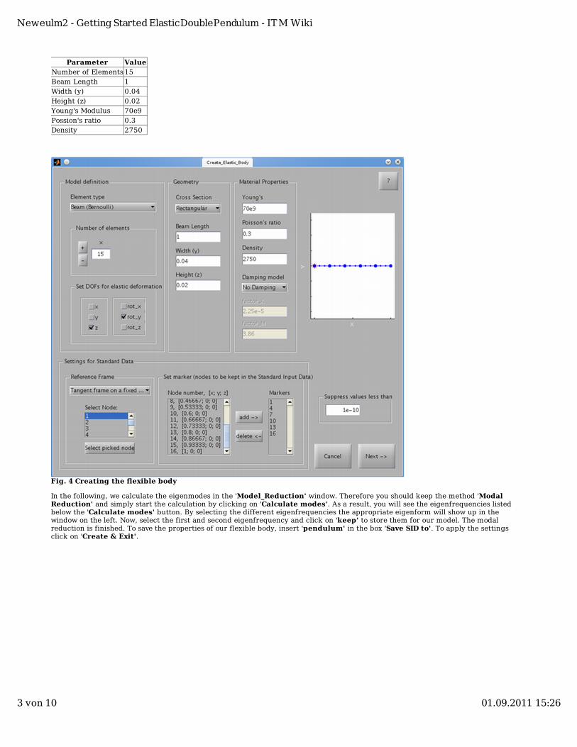
Parameter ValueNumber of Elements 15Beam Length 1Width (y) 0.04Height (z) 0.02Young's Modulus 70e9Possion's ratio 0.3Density 2750
Fig. 4 Creating the flexible body
In the following, we calculate the eigenmodes in the 'Model_Reduction' window. Therefore you should keep the method 'ModalReduction' and simply start the calculation by clicking on 'Calculate modes'. As a result, you will see the eigenfrequencies listedbelow the 'Calculate modes' button. By selecting the different eigenfrequencies the appropriate eigenform will show up in thewindow on the left. Now, select the first and second eigenfrequency and click on 'keep' to store them for our model. The modalreduction is finished. To save the properties of our flexible body, insert 'pendulum' in the box 'Save SID to'. To apply the settingsclick on 'Create & Exit'.
Neweulm2 - Getting Started ElasticDoublePendulum - ITM Wiki
3 von 10 01.09.2011 15:26
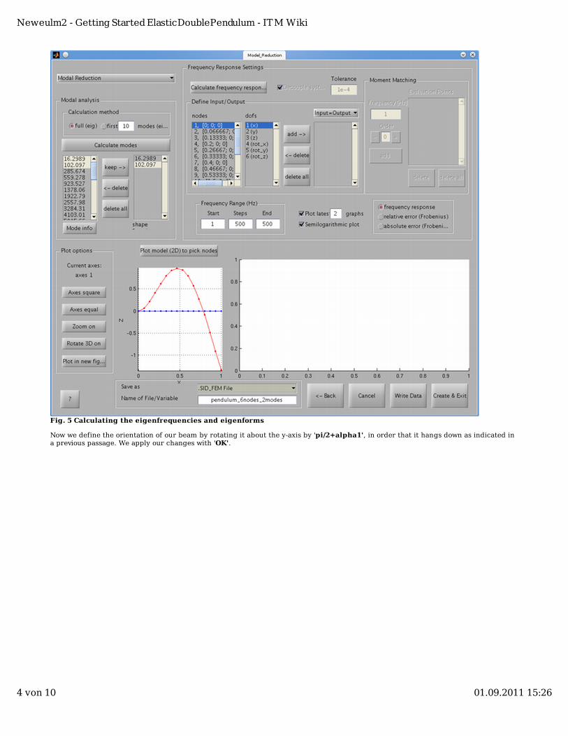
Fig. 5 Calculating the eigenfrequencies and eigenforms
Now we define the orientation of our beam by rotating it about the y-axis by 'pi/2+alpha1', in order that it hangs down as indicated ina previous passage. We apply our changes with 'OK'.
Neweulm2 - Getting Started ElasticDoublePendulum - ITM Wiki
4 von 10 01.09.2011 15:26
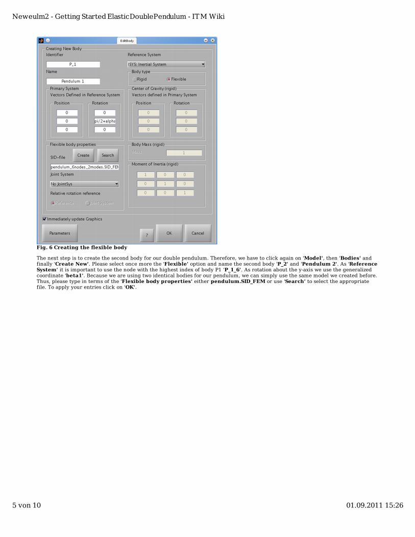
Fig. 6 Creating the flexible body
The next step is to create the second body for our double pendulum. Therefore, we have to click again on 'Model', then 'Bodies' andfinally 'Create New'. Please select once more the 'Flexible' option and name the second body 'P_2' and 'Pendulum 2'. As 'ReferenceSystem' it is important to use the node with the highest index of body P1 'P_1_6'. As rotation about the y-axis we use the generalizedcoordinate 'beta1'. Because we are using two identical bodies for our pendulum, we can simply use the same model we created before.Thus, please type in terms of the 'Flexible body properties' either pendulum.SID_FEM or use 'Search' to select the appropriatefile. To apply your entries click on 'OK'.
Neweulm2 - Getting Started ElasticDoublePendulum - ITM Wiki
5 von 10 01.09.2011 15:26

Fig. 7 Setting up the second body
The elastic beams have been created in the GUI and thus contain information for their graphical representation. The next job is toanimate our newly created system. We shock the lower end of the second body figuratively with a hammer. Thus, we need to insert theappropriate force element. Under 'Model' choose the entry 'Force Elements' and open the window shown in Figure 8 with 'CreateNew'. We identify our force element with 'Shock'. By using 'General' as type, we have the possibility to set up our own individualanimation in the box 'Force Law', in this example:
1/(0.001*sqrt(2*pi))*exp(-(t-0.005)^2/(2*0.001^2))
In addition, we click on 'x' for the direction of our hammer animation. Now set up 'P_2_6' as 'CoordinateSystem 2' to realize the lowerend as point of impact. Apply with 'OK'.
Neweulm2 - Getting Started ElasticDoublePendulum - ITM Wiki
6 von 10 01.09.2011 15:26
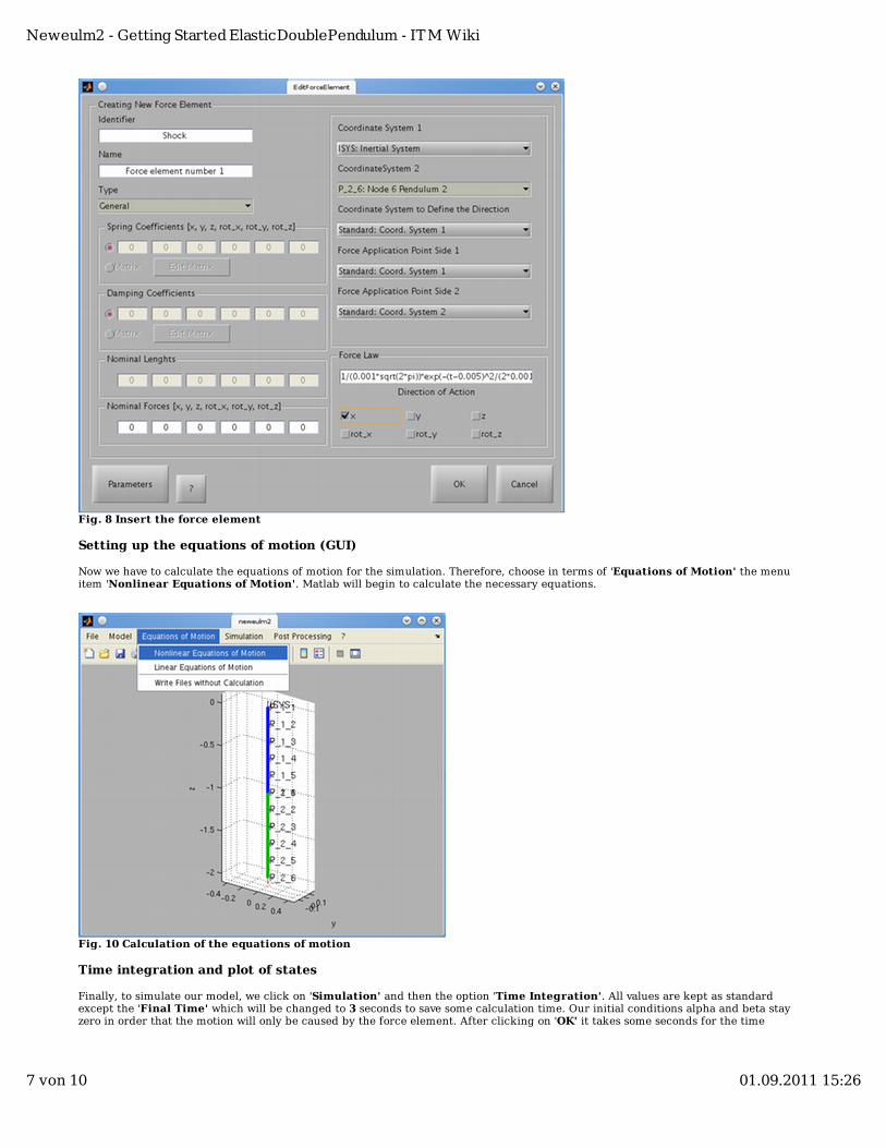
Fig. 8 Insert the force element
Setting up the equations of motion (GUI)
Now we have to calculate the equations of motion for the simulation. Therefore, choose in terms of 'Equations of Motion' the menuitem 'Nonlinear Equations of Motion'. Matlab will begin to calculate the necessary equations.
Fig. 10 Calculation of the equations of motion
Time integration and plot of states
Finally, to simulate our model, we click on 'Simulation' and then the option 'Time Integration'. All values are kept as standardexcept the 'Final Time' which will be changed to 3 seconds to save some calculation time. Our initial conditions alpha and beta stayzero in order that the motion will only be caused by the force element. After clicking on 'OK' it takes some seconds for the time
Neweulm2 - Getting Started ElasticDoublePendulum - ITM Wiki
7 von 10 01.09.2011 15:26
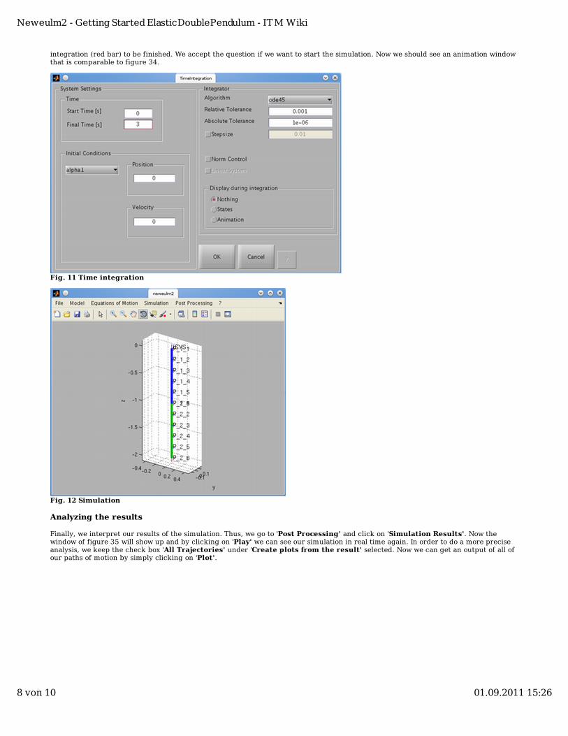
integration (red bar) to be finished. We accept the question if we want to start the simulation. Now we should see an animation windowthat is comparable to figure 34.
Fig. 11 Time integration
Fig. 12 Simulation
Analyzing the results
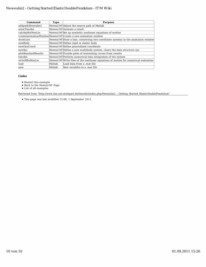
Finally, we interpret our results of the simulation. Thus, we go to 'Post Processing' and click on 'Simulation Results'. Now thewindow of figure 35 will show up and by clicking on 'Play' we can see our simulation in real time again. In order to do a more preciseanalysis, we keep the check box 'All Trajectories' under 'Create plots from the result' selected. Now we can get an output of all ofour paths of motion by simply clicking on 'Plot'.
Neweulm2 - Getting Started ElasticDoublePendulum - ITM Wiki
8 von 10 01.09.2011 15:26
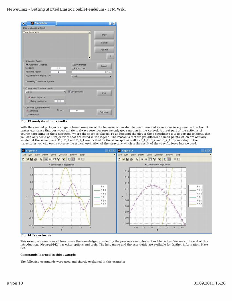
Fig. 13 Analysis of our results
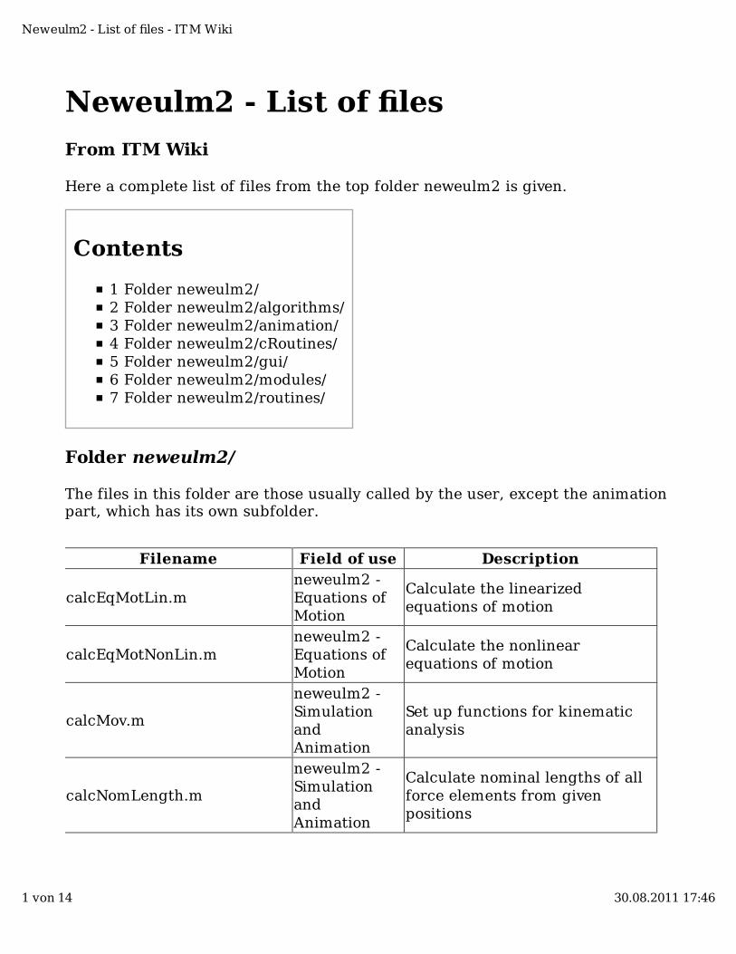
With the created plots you can get a broad overview of the behavior of our double pendulum and its motions in x-,y- and z-direction. Itmakes e.g. sense that our y-coordinate is always zero, because we only got a motion in the xz-level. A great part of the action is ofcourse happening in the x-direction, where the shock is placed. To understand the plot of the x-coordinate it is important to know, thatyou can only see 3 of 6 trajectories that are listed in the legend. The reason is that we got different named points which are actuallylocated at the same place. E.g. P_1 and P_1_1 are located on the same spot as well as P_1_2, P_2 and P_2_1. By zooming in thetrajectories you can easily observe the typical oscillation of the structure which is the result of the specific force law we used.
Fig. 14 Trajectories
This example demonstrated how to use the knowledge provided by the previous examples on flexible bodies. We are at the end of thisintroduction. 'Neweul-M2' has other options and tools. The help menu and the user guide are available for further information. Havefun!
Commands learned in this example
The following commands were used and shortly explained in this example:
Neweulm2 - Getting Started ElasticDoublePendulum - ITM Wiki
9 von 10 01.09.2011 15:26
Command Type PurposeaddpathNeweulm2 Neweul-M² Adjust the search path of MatlabanimTimeInt Neweul-M² Animate a resultcalcEqMotNonLin Neweul-M² Set up symbolic nonlinear equations of motioncreateAnimationWindow Neweul-M² Create a new animation windowdrawLine Neweul-M² Draw a line, connecting two coordinate systems in the animation windownewBody Neweul-M² Define rigid or elastic bodynewGenCoord Neweul-M² Define generalized coordinatenewSys Neweul-M² Define a new multibody system, clears the data structure sysplotStandardResults Neweul-M² Provide plots of interesting curves from resultstimeInt Neweul-M² Perform numerical time integration of the systemwriteMbsNonLin Neweul-M² Write files of the nonlinear equations of motion for numerical evaluationload Matlab Load data from a .mat filesave Matlab Save variables to a .mat file
Links
Restart this exampleBack to the Neweul-M² PageList of all examples
Retrieved from "http://www.itm.uni-stuttgart.de/itmwiki/index.php/Neweulm2_-_Getting_Started_ElasticDoublePendulum"
This page was last modified 12:06, 1 September 2011.
Neweulm2 - Getting Started ElasticDoublePendulum - ITM Wiki
10 von 10 01.09.2011 15:26
Neweulm2 - List of files
From ITM Wiki
Here a complete list of files from the top folder neweulm2 is given.
Contents
1 Folder neweulm2/2 Folder neweulm2/algorithms/3 Folder neweulm2/animation/4 Folder neweulm2/cRoutines/5 Folder neweulm2/gui/6 Folder neweulm2/modules/7 Folder neweulm2/routines/
Folder neweulm2/
The files in this folder are those usually called by the user, except the animationpart, which has its own subfolder.
Filename Field of use Description
calcEqMotLin.mneweulm2 -Equations ofMotion
Calculate the linearizedequations of motion
calcEqMotNonLin.mneweulm2 -Equations ofMotion
Calculate the nonlinearequations of motion
calcMov.m
neweulm2 -SimulationandAnimation
Set up functions for kinematicanalysis
calcNomLength.m
neweulm2 -SimulationandAnimation
Calculate nominal lengths of allforce elements from givenpositions
Neweulm2 - List of files - ITM Wiki
1 von 14 30.08.2011 17:46
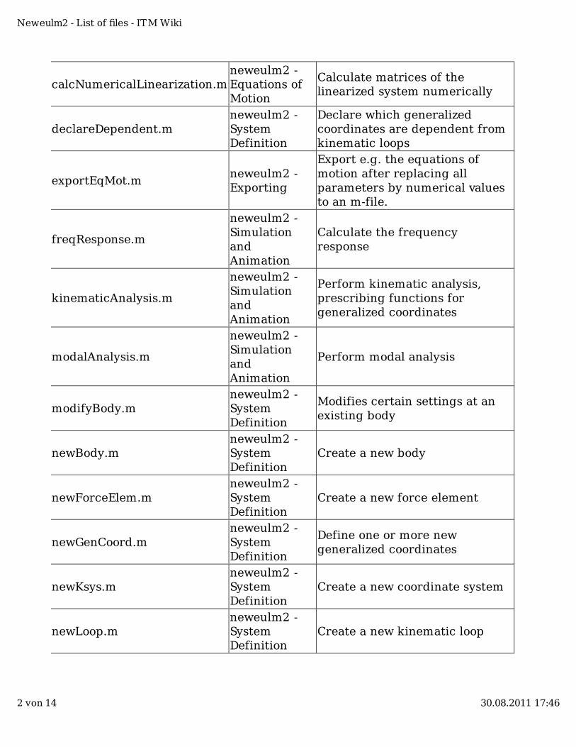
calcNumericalLinearization.mneweulm2 -Equations ofMotion
Calculate matrices of thelinearized system numerically
declareDependent.mneweulm2 -SystemDefinition
Declare which generalizedcoordinates are dependent fromkinematic loops
exportEqMot.mneweulm2 -Exporting
Export e.g. the equations ofmotion after replacing allparameters by numerical valuesto an m-file.
freqResponse.m
neweulm2 -SimulationandAnimation
Calculate the frequencyresponse
kinematicAnalysis.m
neweulm2 -SimulationandAnimation
Perform kinematic analysis,prescribing functions forgeneralized coordinates
modalAnalysis.m
neweulm2 -SimulationandAnimation
Perform modal analysis
modifyBody.mneweulm2 -SystemDefinition
Modifies certain settings at anexisting body
newBody.mneweulm2 -SystemDefinition
Create a new body
newForceElem.mneweulm2 -SystemDefinition
Create a new force element
newGenCoord.mneweulm2 -SystemDefinition
Define one or more newgeneralized coordinates
newKsys.mneweulm2 -SystemDefinition
Create a new coordinate system
newLoop.mneweulm2 -SystemDefinition
Create a new kinematic loop
Neweulm2 - List of files - ITM Wiki
2 von 14 30.08.2011 17:46
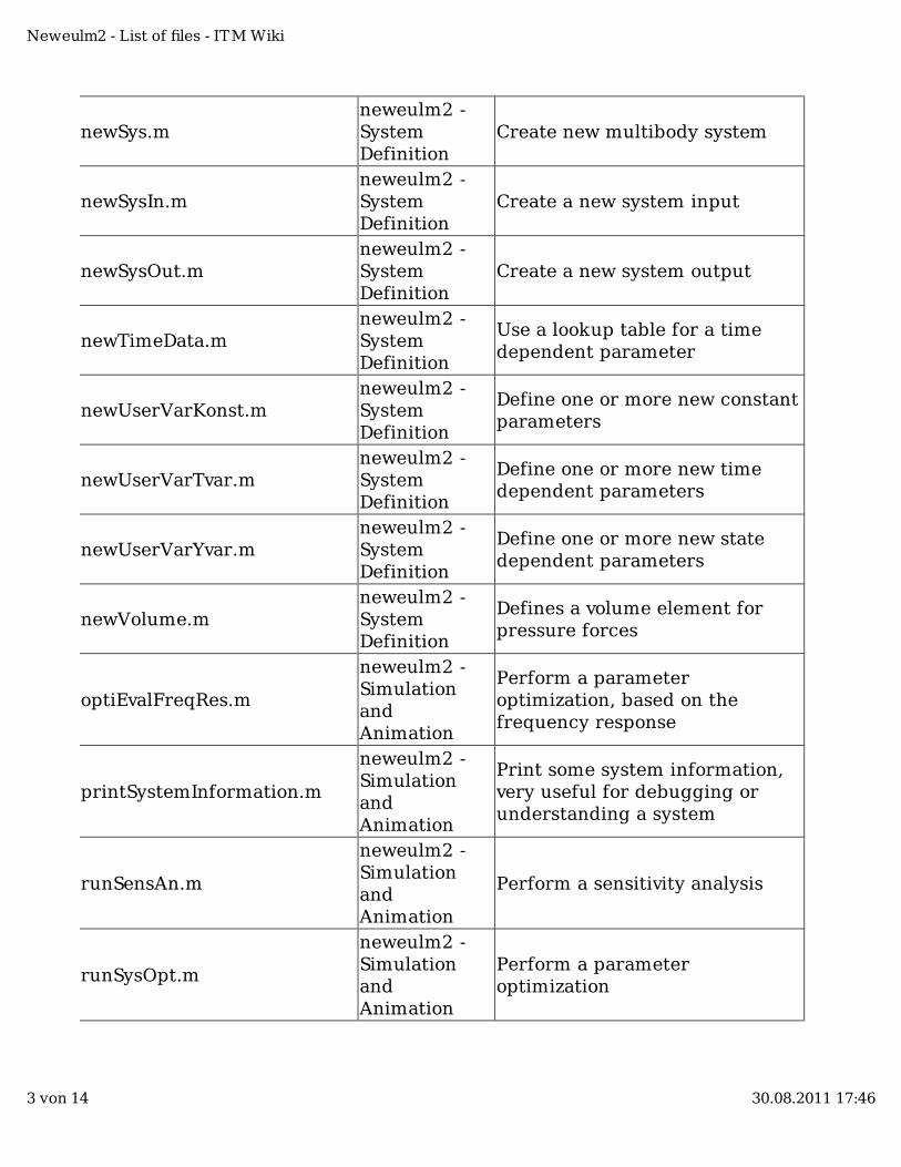
newSys.mneweulm2 -SystemDefinition
Create new multibody system
newSysIn.mneweulm2 -SystemDefinition
Create a new system input
newSysOut.mneweulm2 -SystemDefinition
Create a new system output
newTimeData.mneweulm2 -SystemDefinition
Use a lookup table for a timedependent parameter
newUserVarKonst.mneweulm2 -SystemDefinition
Define one or more new constantparameters
newUserVarTvar.mneweulm2 -SystemDefinition
Define one or more new timedependent parameters
newUserVarYvar.mneweulm2 -SystemDefinition
Define one or more new statedependent parameters
newVolume.mneweulm2 -SystemDefinition
Defines a volume element forpressure forces
optiEvalFreqRes.m
neweulm2 -SimulationandAnimation
Perform a parameteroptimization, based on thefrequency response
printSystemInformation.m
neweulm2 -SimulationandAnimation
Print some system information,very useful for debugging orunderstanding a system
runSensAn.m
neweulm2 -SimulationandAnimation
Perform a sensitivity analysis
runSysOpt.m
neweulm2 -SimulationandAnimation
Perform a parameteroptimization
Neweulm2 - List of files - ITM Wiki
3 von 14 30.08.2011 17:46
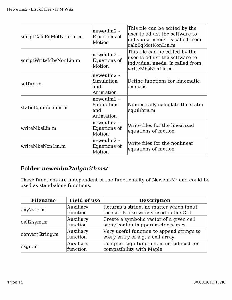
scriptCalcEqMotNonLin.mneweulm2 -Equations ofMotion
This file can be edited by theuser to adjust the software toindividual needs. Is called fromcalcEqMotNonLin.m
scriptWriteMbsNonLin.mneweulm2 -Equations ofMotion
This file can be edited by theuser to adjust the software toindividual needs. Is called fromwriteMbsNonLin.m
setfun.m
neweulm2 -SimulationandAnimation
Define functions for kinematicanalysis
staticEquilibrium.m
neweulm2 -SimulationandAnimation
Numerically calculate the staticequilibrium
writeMbsLin.mneweulm2 -Equations ofMotion
Write files for the linearizedequations of motion
writeMbsNonLin.mneweulm2 -Equations ofMotion
Write files for the nonlinearequations of motion
Folder neweulm2/algorithms/
These functions are independent of the functionality of Neweul-M² and could beused as stand-alone functions.
Filename Field of use Description
any2str.mAuxiliaryfunction
Returns a string, no matter which inputformat. Is also widely used in the GUI
cell2sym.mAuxiliaryfunction
Create a symbolic vector of a given cellarray containing parameter names
convertString.mAuxiliaryfunction
Very useful function to append strings toevery entry of e.g. a cell array
csgn.mAuxiliaryfunction
Complex sign function, is introduced forcompatibility with Maple
Neweulm2 - List of files - ITM Wiki
4 von 14 30.08.2011 17:46
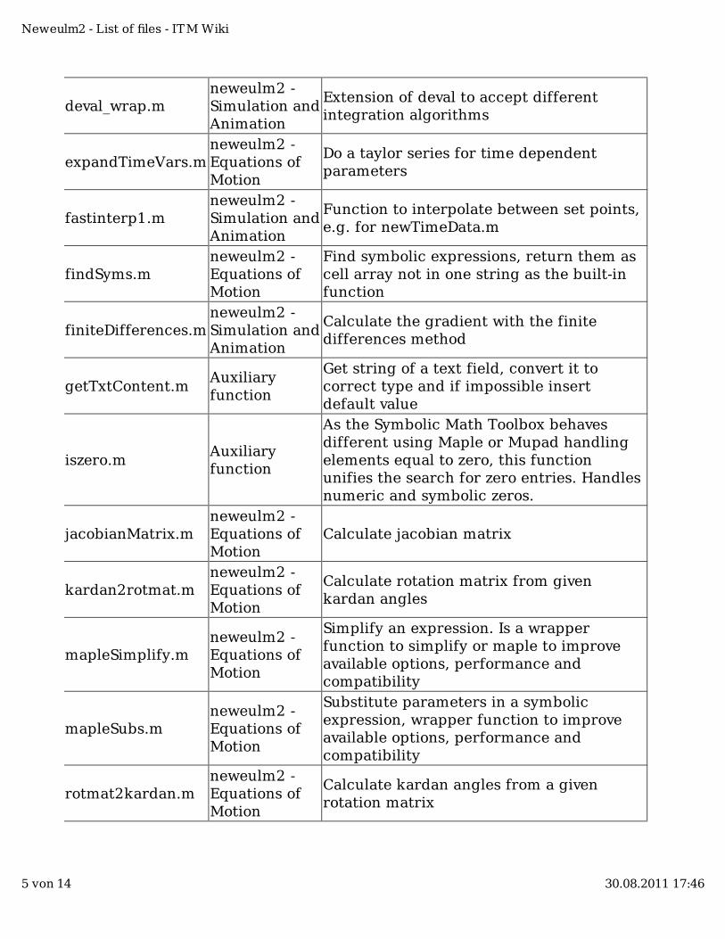
deval_wrap.mneweulm2 -Simulation andAnimation
Extension of deval to accept differentintegration algorithms
expandTimeVars.mneweulm2 -Equations ofMotion
Do a taylor series for time dependentparameters
fastinterp1.mneweulm2 -Simulation andAnimation
Function to interpolate between set points,e.g. for newTimeData.m
findSyms.mneweulm2 -Equations ofMotion
Find symbolic expressions, return them ascell array not in one string as the built-infunction
finiteDifferences.mneweulm2 -Simulation andAnimation
Calculate the gradient with the finitedifferences method
getTxtContent.mAuxiliaryfunction
Get string of a text field, convert it tocorrect type and if impossible insertdefault value
iszero.mAuxiliaryfunction
As the Symbolic Math Toolbox behavesdifferent using Maple or Mupad handlingelements equal to zero, this functionunifies the search for zero entries. Handlesnumeric and symbolic zeros.
jacobianMatrix.mneweulm2 -Equations ofMotion
Calculate jacobian matrix
kardan2rotmat.mneweulm2 -Equations ofMotion
Calculate rotation matrix from givenkardan angles
mapleSimplify.mneweulm2 -Equations ofMotion
Simplify an expression. Is a wrapperfunction to simplify or maple to improveavailable options, performance andcompatibility
mapleSubs.mneweulm2 -Equations ofMotion
Substitute parameters in a symbolicexpression, wrapper function to improveavailable options, performance andcompatibility
rotmat2kardan.mneweulm2 -Equations ofMotion
Calculate kardan angles from a givenrotation matrix
Neweulm2 - List of files - ITM Wiki
5 von 14 30.08.2011 17:46
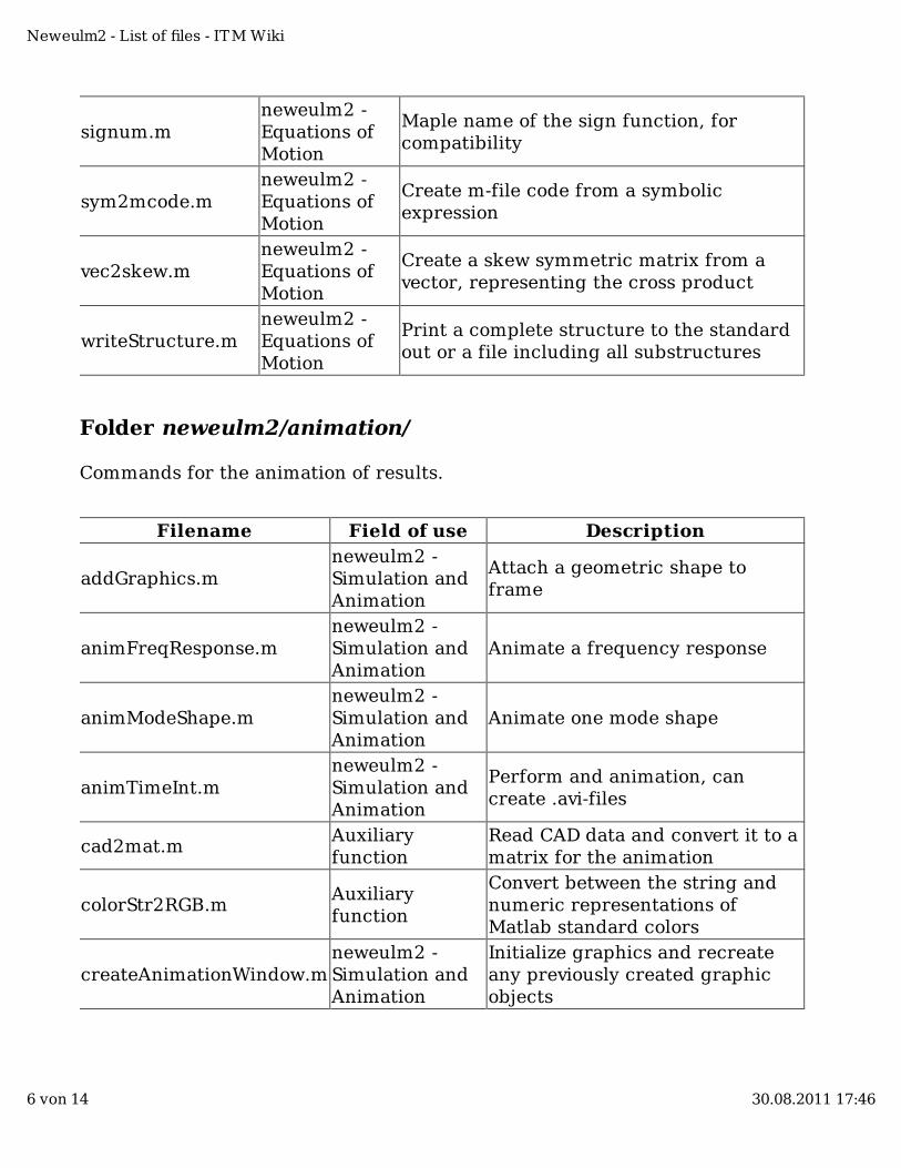
signum.mneweulm2 -Equations ofMotion
Maple name of the sign function, forcompatibility
sym2mcode.mneweulm2 -Equations ofMotion
Create m-file code from a symbolicexpression
vec2skew.mneweulm2 -Equations ofMotion
Create a skew symmetric matrix from avector, representing the cross product
writeStructure.mneweulm2 -Equations ofMotion
Print a complete structure to the standardout or a file including all substructures
Folder neweulm2/animation/
Commands for the animation of results.
Filename Field of use Description
addGraphics.mneweulm2 -Simulation andAnimation
Attach a geometric shape toframe
animFreqResponse.mneweulm2 -Simulation andAnimation
Animate a frequency response
animModeShape.mneweulm2 -Simulation andAnimation
Animate one mode shape
animTimeInt.mneweulm2 -Simulation andAnimation
Perform and animation, cancreate .avi-files
cad2mat.mAuxiliaryfunction
Read CAD data and convert it to amatrix for the animation
colorStr2RGB.mAuxiliaryfunction
Convert between the string andnumeric representations ofMatlab standard colors
createAnimationWindow.mneweulm2 -Simulation andAnimation
Initialize graphics and recreateany previously created graphicobjects
Neweulm2 - List of files - ITM Wiki
6 von 14 30.08.2011 17:46
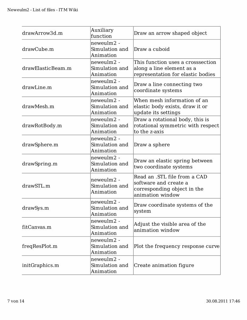
drawArrow3d.mAuxiliaryfunction
Draw an arrow shaped object
drawCube.mneweulm2 -Simulation andAnimation
Draw a cuboid
drawElasticBeam.mneweulm2 -Simulation andAnimation
This function uses a crosssectionalong a line element as arepresentation for elastic bodies
drawLine.mneweulm2 -Simulation andAnimation
Draw a line connecting twocoordinate systems
drawMesh.mneweulm2 -Simulation andAnimation
When mesh information of anelastic body exists, draw it orupdate its settings
drawRotBody.mneweulm2 -Simulation andAnimation
Draw a rotational body, this isrotational symmetric with respectto the z-axis
drawSphere.mneweulm2 -Simulation andAnimation
Draw a sphere
drawSpring.mneweulm2 -Simulation andAnimation
Draw an elastic spring betweentwo coordinate systems
drawSTL.mneweulm2 -Simulation andAnimation
Read an .STL file from a CADsoftware and create acorresponding object in theanimation window
drawSys.mneweulm2 -Simulation andAnimation
Draw coordinate systems of thesystem
fitCanvas.mneweulm2 -Simulation andAnimation
Adjust the visible area of theanimation window
freqResPlot.mneweulm2 -Simulation andAnimation
Plot the frequency response curve
initGraphics.mneweulm2 -Simulation andAnimation
Create animation figure
Neweulm2 - List of files - ITM Wiki
7 von 14 30.08.2011 17:46
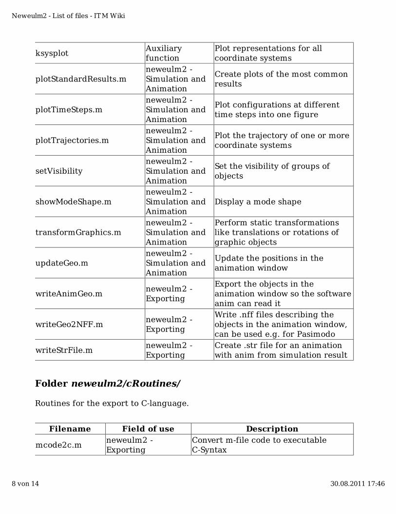
ksysplotAuxiliaryfunction
Plot representations for allcoordinate systems
plotStandardResults.mneweulm2 -Simulation andAnimation
Create plots of the most commonresults
plotTimeSteps.mneweulm2 -Simulation andAnimation
Plot configurations at differenttime steps into one figure
plotTrajectories.mneweulm2 -Simulation andAnimation
Plot the trajectory of one or morecoordinate systems
setVisibilityneweulm2 -Simulation andAnimation
Set the visibility of groups ofobjects
showModeShape.mneweulm2 -Simulation andAnimation
Display a mode shape
transformGraphics.mneweulm2 -Simulation andAnimation
Perform static transformationslike translations or rotations ofgraphic objects
updateGeo.mneweulm2 -Simulation andAnimation
Update the positions in theanimation window
writeAnimGeo.mneweulm2 -Exporting
Export the objects in theanimation window so the softwareanim can read it
writeGeo2NFF.mneweulm2 -Exporting
Write .nff files describing theobjects in the animation window,can be used e.g. for Pasimodo
writeStrFile.mneweulm2 -Exporting
Create .str file for an animationwith anim from simulation result
Folder neweulm2/cRoutines/
Routines for the export to C-language.
Filename Field of use Description
mcode2c.mneweulm2 -Exporting
Convert m-file code to executableC-Syntax
Neweulm2 - List of files - ITM Wiki
8 von 14 30.08.2011 17:46
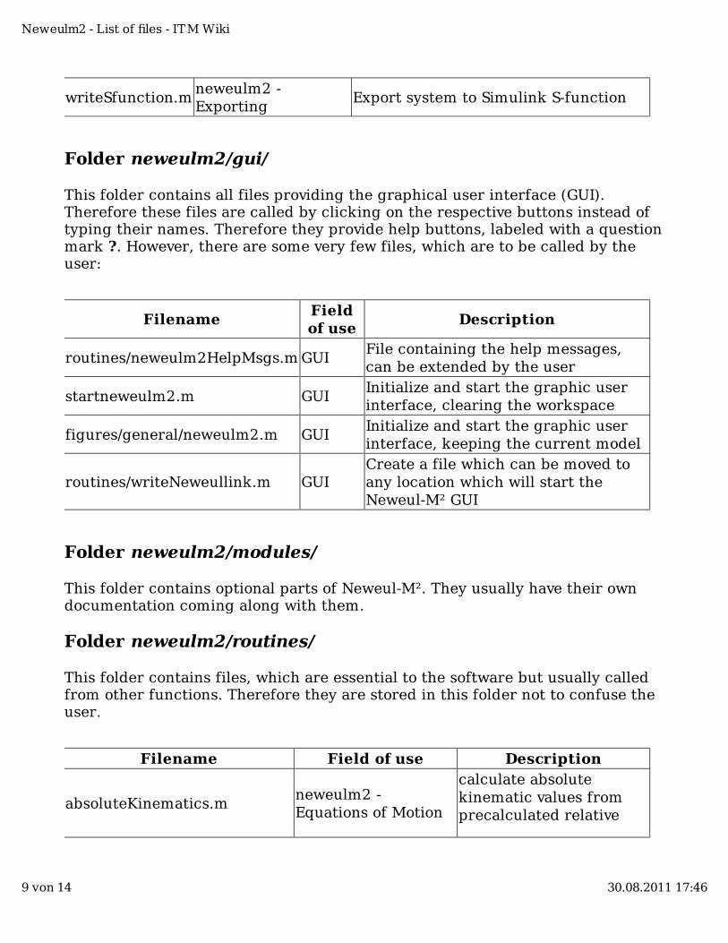
writeSfunction.mneweulm2 -Exporting
Export system to Simulink S-function
Folder neweulm2/gui/
This folder contains all files providing the graphical user interface (GUI).Therefore these files are called by clicking on the respective buttons instead oftyping their names. Therefore they provide help buttons, labeled with a questionmark ?. However, there are some very few files, which are to be called by theuser:
FilenameFieldof use
Description
routines/neweulm2HelpMsgs.m GUIFile containing the help messages,can be extended by the user
startneweulm2.m GUIInitialize and start the graphic userinterface, clearing the workspace
figures/general/neweulm2.m GUIInitialize and start the graphic userinterface, keeping the current model
routines/writeNeweullink.m GUICreate a file which can be moved toany location which will start theNeweul-M² GUI
Folder neweulm2/modules/
This folder contains optional parts of Neweul-M². They usually have their owndocumentation coming along with them.
Folder neweulm2/routines/
This folder contains files, which are essential to the software but usually calledfrom other functions. Therefore they are stored in this folder not to confuse theuser.
Filename Field of use Description
absoluteKinematics.mneweulm2 -Equations of Motion
calculate absolutekinematic values fromprecalculated relative
Neweulm2 - List of files - ITM Wiki
9 von 14 30.08.2011 17:46
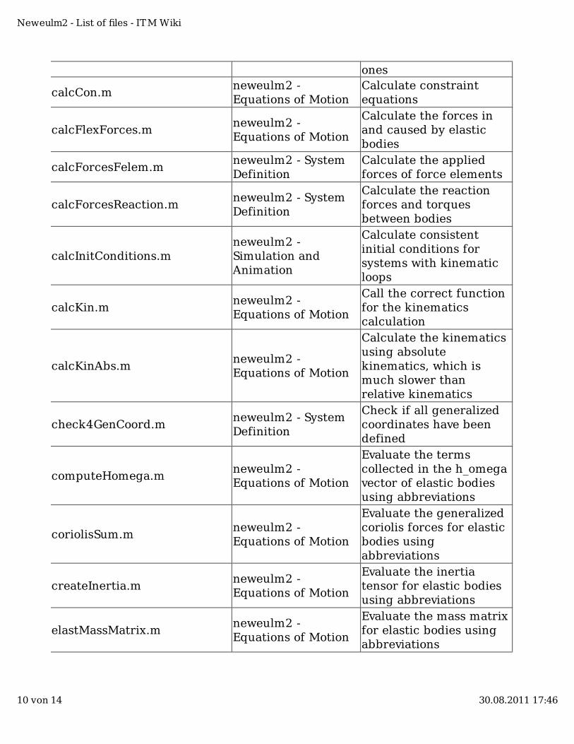
ones
calcCon.mneweulm2 -Equations of Motion
Calculate constraintequations
calcFlexForces.mneweulm2 -Equations of Motion
Calculate the forces inand caused by elasticbodies
calcForcesFelem.mneweulm2 - SystemDefinition
Calculate the appliedforces of force elements
calcForcesReaction.mneweulm2 - SystemDefinition
Calculate the reactionforces and torquesbetween bodies
calcInitConditions.mneweulm2 -Simulation andAnimation
Calculate consistentinitial conditions forsystems with kinematicloops
calcKin.mneweulm2 -Equations of Motion
Call the correct functionfor the kinematicscalculation
calcKinAbs.mneweulm2 -Equations of Motion
Calculate the kinematicsusing absolutekinematics, which ismuch slower thanrelative kinematics
check4GenCoord.mneweulm2 - SystemDefinition
Check if all generalizedcoordinates have beendefined
computeHomega.mneweulm2 -Equations of Motion
Evaluate the termscollected in the h_omegavector of elastic bodiesusing abbreviations
coriolisSum.mneweulm2 -Equations of Motion
Evaluate the generalizedcoriolis forces for elasticbodies usingabbreviations
createInertia.mneweulm2 -Equations of Motion
Evaluate the inertiatensor for elastic bodiesusing abbreviations
elastMassMatrix.mneweulm2 -Equations of Motion
Evaluate the mass matrixfor elastic bodies usingabbreviations
Neweulm2 - List of files - ITM Wiki
10 von 14 30.08.2011 17:46
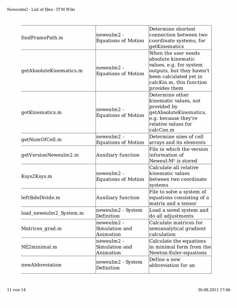
findFramePath.mneweulm2 -Equations of Motion
Determine shortestconnection between twocoordinate systems, forgetKinematics
getAbsoluteKinematics.mneweulm2 -Equations of Motion
When the user needsabsolute kinematicvalues, e.g. for systemoutputs, but they haven'tbeen calculated yet incalcKin.m, this functionprovides them
getKinematics.mneweulm2 -Equations of Motion
Determine otherkinematic values, notprovided bygetAbsoluteKinematics,e.g. because they'rerelative values forcalcCon.m
getNumOfCell.mneweulm2 -Equations of Motion
Determine sizes of cellarrays and its elements
getVersionNeweulm2.m Auxiliary functionFile in which the versioninformation ofNeweul-M² is stored
Ksys2Ksys.mneweulm2 -Equations of Motion
Calculate all relativekinematic valuesbetween two coordinatesystems
leftSideDivide.m Auxiliary functionFile to solve a system ofequations consisting of amatrix and a tensor
load_neweulm2_System.mneweulm2 - SystemDefinition
Load a saved system anddo all adjustments
Matrices_grad.mneweulm2 -Simulation andAnimation
Calculate matrices forsemianalytical gradientcalculation
NE2minimal.mneweulm2 -Simulation andAnimation
Calculate the equationsin minimal form from theNewton-Euler-equations
newAbbreviationneweulm2 - SystemDefinition
Define a newabbreviation for an
Neweulm2 - List of files - ITM Wiki
11 von 14 30.08.2011 17:46
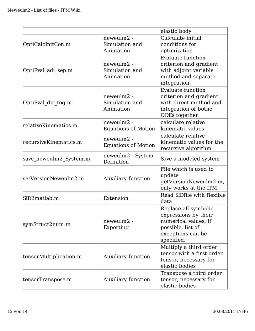
elastic body
OptiCalcInitCon.mneweulm2 -Simulation andAnimation
Calculate initialconditions foroptimization
OptiEval_adj_sep.mneweulm2 -Simulation andAnimation
Evaluate functioncriterion and gradientwith adjoint variablemethod and separateintegration.
OptiEval_dir_tog.mneweulm2 -Simulation andAnimation
Evaluate functioncriterion and gradientwith direct method andintegration of botheODEs together.
relativeKinematics.mneweulm2 -Equations of Motion
calculate relativekinematic values
recursiveKinematics.mneweulm2 -Equations of Motion
calculate relativekinematic values for therecursive algorithm
save_neweulm2_System.mneweulm2 - SystemDefinition
Save a modeled system
setVersionNeweulm2.m Auxiliary function
File which is used toupdategetVersionNeweulm2.m,only works at the ITM
SID2matlab.m ExtensionRead SIDfile with flexibledata
symStruct2num.mneweulm2 -Exporting
Replace all symbolicexpressions by theirnumerical values, ifpossible, list ofexceptions can bespecified.
tensorMultiplication.m Auxiliary function
Multiply a third ordertensor with a first ordertensor, necessary forelastic bodies
tensorTranspose.m Auxiliary functionTranspose a third ordertensor, necessary forelastic bodies
Neweulm2 - List of files - ITM Wiki
12 von 14 30.08.2011 17:46
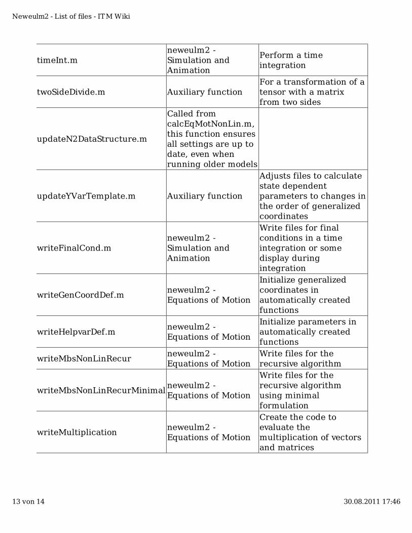
timeInt.mneweulm2 -Simulation andAnimation
Perform a timeintegration
twoSideDivide.m Auxiliary functionFor a transformation of atensor with a matrixfrom two sides
updateN2DataStructure.m
Called fromcalcEqMotNonLin.m,this function ensuresall settings are up todate, even whenrunning older models
updateYVarTemplate.m Auxiliary function
Adjusts files to calculatestate dependentparameters to changes inthe order of generalizedcoordinates
writeFinalCond.mneweulm2 -Simulation andAnimation
Write files for finalconditions in a timeintegration or somedisplay duringintegration
writeGenCoordDef.mneweulm2 -Equations of Motion
Initialize generalizedcoordinates inautomatically createdfunctions
writeHelpvarDef.mneweulm2 -Equations of Motion
Initialize parameters inautomatically createdfunctions
writeMbsNonLinRecurneweulm2 -Equations of Motion
Write files for therecursive algorithm
writeMbsNonLinRecurMinimalneweulm2 -Equations of Motion
Write files for therecursive algorithmusing minimalformulation
writeMultiplicationneweulm2 -Equations of Motion
Create the code toevaluate themultiplication of vectorsand matrices
Neweulm2 - List of files - ITM Wiki
13 von 14 30.08.2011 17:46
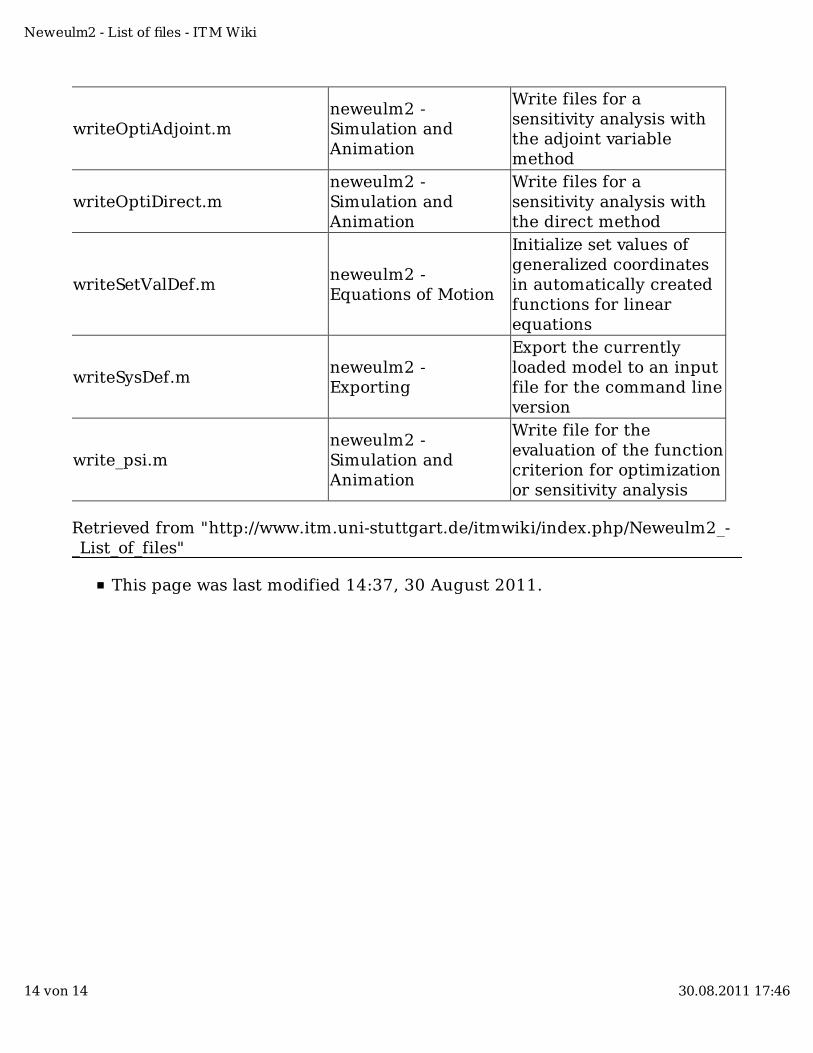
writeOptiAdjoint.mneweulm2 -Simulation andAnimation
Write files for asensitivity analysis withthe adjoint variablemethod
writeOptiDirect.mneweulm2 -Simulation andAnimation
Write files for asensitivity analysis withthe direct method
writeSetValDef.mneweulm2 -Equations of Motion
Initialize set values ofgeneralized coordinatesin automatically createdfunctions for linearequations
writeSysDef.mneweulm2 -Exporting
Export the currentlyloaded model to an inputfile for the command lineversion
write_psi.mneweulm2 -Simulation andAnimation
Write file for theevaluation of the functioncriterion for optimizationor sensitivity analysis
Retrieved from "http://www.itm.uni-stuttgart.de/itmwiki/index.php/Neweulm2_-_List_of_files"
This page was last modified 14:37, 30 August 2011.
Neweulm2 - List of files - ITM Wiki
14 von 14 30.08.2011 17:46
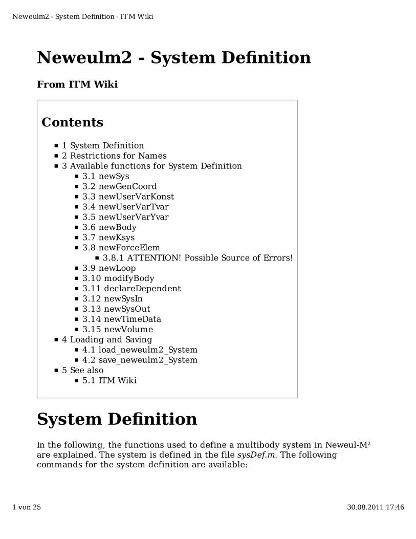
Neweulm2 - System Definition
From ITM Wiki
Contents
1 System Definition2 Restrictions for Names3 Available functions for System Definition
3.1 newSys3.2 newGenCoord3.3 newUserVarKonst3.4 newUserVarTvar3.5 newUserVarYvar3.6 newBody3.7 newKsys3.8 newForceElem
3.8.1 ATTENTION! Possible Source of Errors!3.9 newLoop3.10 modifyBody3.11 declareDependent3.12 newSysIn3.13 newSysOut3.14 newTimeData3.15 newVolume
4 Loading and Saving4.1 load_neweulm2_System4.2 save_neweulm2_System
5 See also5.1 ITM Wiki
System DefinitionIn the following, the functions used to define a multibody system in Neweul-M²are explained. The system is defined in the file sysDef.m. The followingcommands for the system definition are available:
Neweulm2 - System Definition - ITM Wiki
1 von 25 30.08.2011 17:46
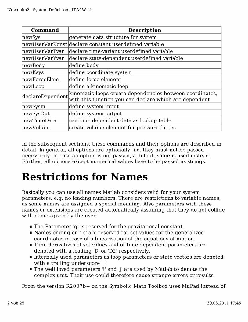
Command DescriptionnewSys generate data structure for systemnewUserVarKonst declare constant userdefined variablenewUserVarTvar declare time-variant userdefined variablenewUserVarYvar declare state-dependent userdefined variablenewBody define bodynewKsys define coordinate systemnewForceElem define force elementnewLoop define a kinematic loop
declareDependentkinematic loops create dependencies between coordinates,with this function you can declare which are dependent
newSysIn define system inputnewSysOut define system outputnewTimeData use time dependent data as lookup tablenewVolume create volume element for pressure forces
In the subsequent sections, these commands and their options are described indetail. In general, all options are optionally, i.e. they must not be passednecessarily. In case an option is not passed, a default value is used instead.Further, all options except numerical values have to be passed as strings.
Restrictions for NamesBasically you can use all names Matlab considers valid for your systemparameters, e.g. no leading numbers. There are restrictions to variable names,as some names are assigned a special meaning. Also parameters with thesenames or extensions are created automatically assuming that they do not collidewith names given by the user.
The Parameter 'g' is reserved for the gravitational constant.Names ending on '_s' are reserved for set values for the generalizedcoordinates in case of a linearization of the equations of motion.Time derivatives of set values and of time dependent parameters aredenoted with a leading 'D' or 'D2' respectively.Internally used parameters as loop parameters or state vectors are denotedwith a trailing underscore '_'.The well loved parameters 'i' and 'j' are used by Matlab to denote thecomplex unit. Their use could therefore cause strange errors or results.
From the version R2007b+ on the Symbolic Math Toolbox uses MuPad instead of
Neweulm2 - System Definition - ITM Wiki
2 von 25 30.08.2011 17:46
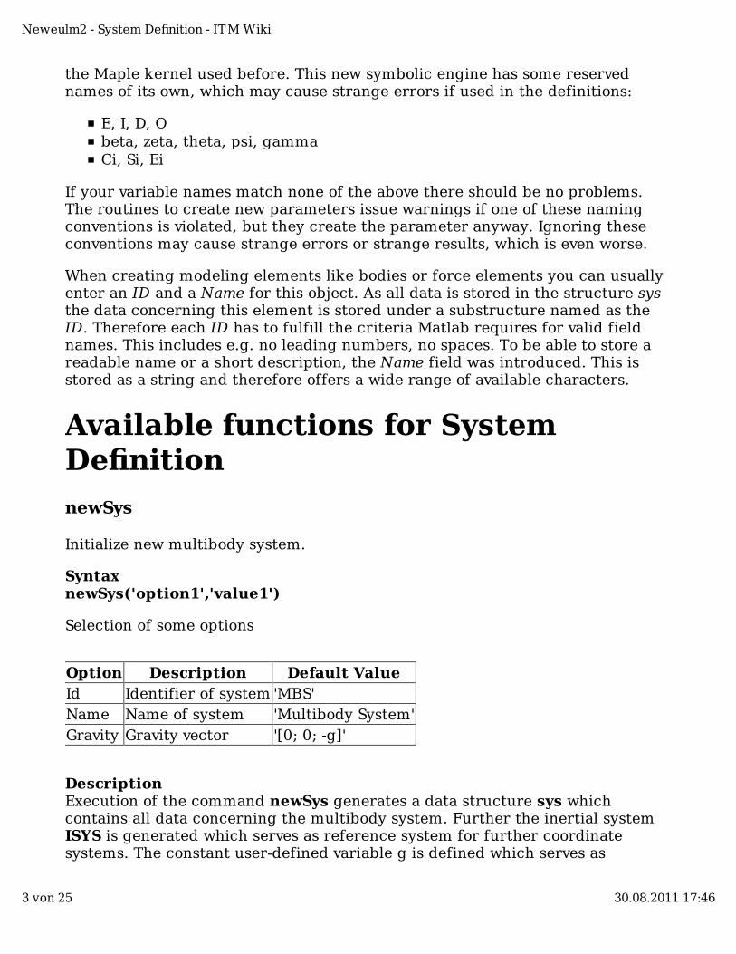
the Maple kernel used before. This new symbolic engine has some reservednames of its own, which may cause strange errors if used in the definitions:
E, I, D, Obeta, zeta, theta, psi, gammaCi, Si, Ei
If your variable names match none of the above there should be no problems.The routines to create new parameters issue warnings if one of these namingconventions is violated, but they create the parameter anyway. Ignoring theseconventions may cause strange errors or strange results, which is even worse.
When creating modeling elements like bodies or force elements you can usuallyenter an ID and a Name for this object. As all data is stored in the structure systhe data concerning this element is stored under a substructure named as theID. Therefore each ID has to fulfill the criteria Matlab requires for valid fieldnames. This includes e.g. no leading numbers, no spaces. To be able to store areadable name or a short description, the Name field was introduced. This isstored as a string and therefore offers a wide range of available characters.
Available functions for SystemDefinition
newSys
Initialize new multibody system.
SyntaxnewSys('option1','value1')
Selection of some options
Option Description Default ValueId Identifier of system 'MBS'Name Name of system 'Multibody System'Gravity Gravity vector '[0; 0; -g]'
DescriptionExecution of the command newSys generates a data structure sys whichcontains all data concerning the multibody system. Further the inertial systemISYS is generated which serves as reference system for further coordinatesystems. The constant user-defined variable g is defined which serves as
Neweulm2 - System Definition - ITM Wiki
3 von 25 30.08.2011 17:46
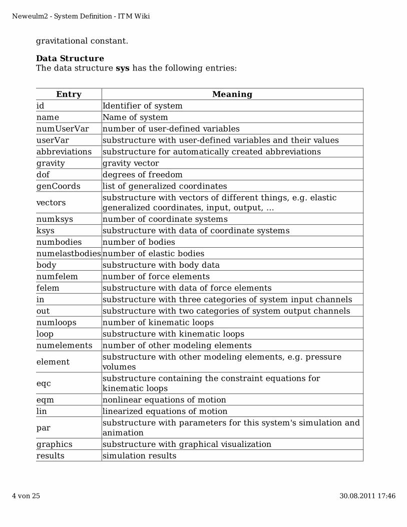
gravitational constant.
Data StructureThe data structure sys has the following entries:
Entry Meaningid Identifier of systemname Name of systemnumUserVar number of user-defined variablesuserVar substructure with user-defined variables and their valuesabbreviations substructure for automatically created abbreviationsgravity gravity vectordof degrees of freedomgenCoords list of generalized coordinates
vectorssubstructure with vectors of different things, e.g. elasticgeneralized coordinates, input, output, ...
numksys number of coordinate systemsksys substructure with data of coordinate systemsnumbodies number of bodiesnumelastbodies number of elastic bodiesbody substructure with body datanumfelem number of force elementsfelem substructure with data of force elementsin substructure with three categories of system input channelsout substructure with two categories of system output channelsnumloops number of kinematic loopsloop substructure with kinematic loopsnumelements number of other modeling elements
elementsubstructure with other modeling elements, e.g. pressurevolumes
eqcsubstructure containing the constraint equations forkinematic loops
eqm nonlinear equations of motionlin linearized equations of motion
parsubstructure with parameters for this system's simulation andanimation
graphics substructure with graphical visualizationresults simulation results
Neweulm2 - System Definition - ITM Wiki
4 von 25 30.08.2011 17:46
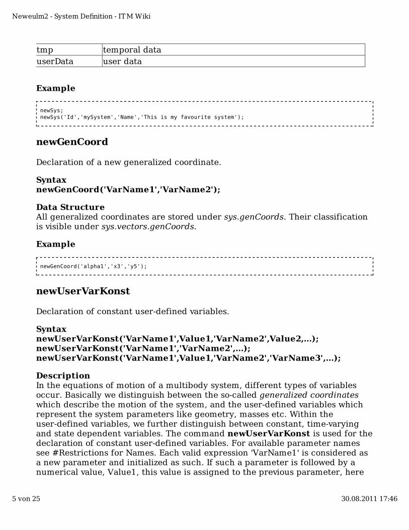
tmp temporal datauserData user data
Example
newSys; newSys('Id','mySystem','Name','This is my favourite system');
newGenCoord
Declaration of a new generalized coordinate.
SyntaxnewGenCoord('VarName1','VarName2');
Data StructureAll generalized coordinates are stored under sys.genCoords. Their classificationis visible under sys.vectors.genCoords.
Example
newGenCoord('alpha1','x3','y5');
newUserVarKonst
Declaration of constant user-defined variables.
SyntaxnewUserVarKonst('VarName1',Value1,'VarName2',Value2,...);newUserVarKonst('VarName1','VarName2',...);newUserVarKonst('VarName1',Value1,'VarName2','VarName3',...);
DescriptionIn the equations of motion of a multibody system, different types of variablesoccur. Basically we distinguish between the so-called generalized coordinateswhich describe the motion of the system, and the user-defined variables whichrepresent the system parameters like geometry, masses etc. Within theuser-defined variables, we further distinguish between constant, time-varyingand state dependent variables. The command newUserVarKonst is used for thedeclaration of constant user-defined variables. For available parameter namessee #Restrictions for Names. Each valid expression 'VarName1' is considered asa new parameter and initialized as such. If such a parameter is followed by anumerical value, Value1, this value is assigned to the previous parameter, here
Neweulm2 - System Definition - ITM Wiki
5 von 25 30.08.2011 17:46
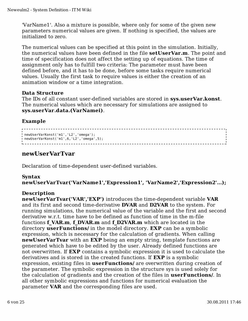
'VarName1'. Also a mixture is possible, where only for some of the given newparameters numerical values are given. If nothing is specified, the values areinitialized to zero.
The numerical values can be specified at this point in the simulation. Initially,the numerical values have been defined in the file setUserVar.m. The point andtime of specification does not affect the setting up of equations. The time ofassignment only has to fulfill two criteria: The parameter must have beendefined before, and it has to be done, before some tasks require numericalvalues. Usually the first task to require values is either the creation of ananimation window or a time integration.
Data StructureThe IDs of all constant user-defined variables are stored in sys.userVar.konst.The numerical values which are necessary for simulations are assigned tosys.userVar.data.(VarNamei).
Example
newUserVarKonst('m1','L2','omega'); newUserVarKonst('m1',6,'L2','omega',5);
newUserVarTvar
Declaration of time-dependent user-defined variables.
SyntaxnewUserVarTvar('VarName1','Expression1', 'VarName2','Expression2'...);
DescriptionnewUserVarTvar('VAR','EXP') introduces the time-dependent variable VARand its first and second time-derivative DVAR and D2VAR to the system. Forrunning simulations, the numerical value of the variable and the first and secondderivative w.r.t. time have to be defined as function of time in the m-filefunctions f_VAR.m, f_DVAR.m and f_D2VAR.m which are located in thedirectory userFunctions/ in the model directory. EXP can be a symbolicexpression, which is necessary for the calculation of gradients. When callingnewUserVarTvar with an EXP being an empty string, template functions aregenerated which have to be edited by the user. Already defined functions arenot overwritten. If EXP contains a symbolic expression it is used to calculate thederivatives and is stored in the created functions. If EXP is a symbolicexpression, existing files in userFunctions/ are overwritten during creation ofthe parameter. The symbolic expression in the structure sys is used solely forthe calculation of gradients and the creation of the files in userFunctions/. Inall other symbolic expressions and functions for numerical evaluation theparameter VAR and the corresponding files are used.
Neweulm2 - System Definition - ITM Wiki
6 von 25 30.08.2011 17:46
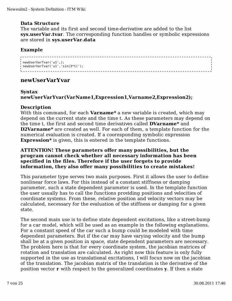
Data StructureThe variable and its first and second time-derivative are added to the listsys.userVar.tvar. The corresponding function handles or symbolic expressionsare stored in sys.userVar.data
Example
newUserVarTvar('u1',); newUserVarTvar('u1','sin(3*t)');
newUserVarYvar
SyntaxnewUserVarYvar(VarName1,Expression1,Varname2,Expression2);
DescriptionWith this command, for each Varname* a new variable is created, which maydepend on the current state and the time t. As these parameters may depend onthe time t, the first and second time derivatives called DVarname* andD2Varname* are created as well. For each of them, a template function for thenumerical evaluation is created. If a cooresponding symbolic expressionExpression* is given, this is entered in the template functions.
ATTENTION! These parameters offer many possibilities, but theprogram cannot check whether all necessary information has beenspecified in the files. Therefore if the user forgets to provideinformation, they also offer many possibilities to create mistakes!
This parameter type serves two main purposes. First it allows the user to definenonlinear force laws. For this instead of a constant stiffness or dampingparameter, such a state dependent parameter is used. In the template functionthe user usually has to call the functions providing positions and velocities ofcoordinate systems. From these, relative position and velocity vectors may becalculated, necessary for the evaluation of the stiffness or damping for a givenstate.
The second main use is to define state dependent excitations, like a street-bumpfor a car model, which will be used as an example in the following explanations.For a constant speed of the car such a bump could be modeled with timedependent parameters. But if the car may have varying velocity and the bumpshall be at a given position in space, state dependent parameters are necessary.The problem here is that for every coordinate system, the jacobian matrices ofrotation and translation are calculated. As right now this feature is only fullysupported in the use as translational excitations, I will focus now on the jacobianof the translation. The jacobian matrix of the translation is the derivative of theposition vector r with respect to the generalized coordinates y. If then a state
Neweulm2 - System Definition - ITM Wiki
7 von 25 30.08.2011 17:46
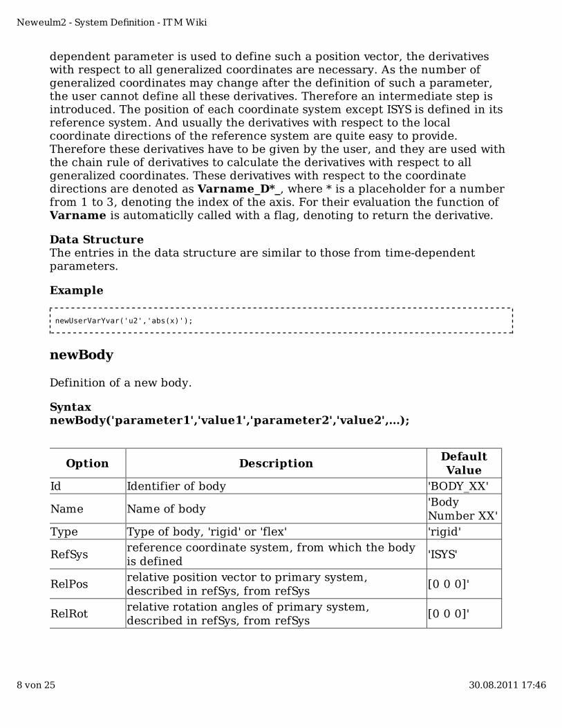
dependent parameter is used to define such a position vector, the derivativeswith respect to all generalized coordinates are necessary. As the number ofgeneralized coordinates may change after the definition of such a parameter,the user cannot define all these derivatives. Therefore an intermediate step isintroduced. The position of each coordinate system except ISYS is defined in itsreference system. And usually the derivatives with respect to the localcoordinate directions of the reference system are quite easy to provide.Therefore these derivatives have to be given by the user, and they are used withthe chain rule of derivatives to calculate the derivatives with respect to allgeneralized coordinates. These derivatives with respect to the coordinatedirections are denoted as Varname_D*_, where * is a placeholder for a numberfrom 1 to 3, denoting the index of the axis. For their evaluation the function ofVarname is automaticlly called with a flag, denoting to return the derivative.
Data StructureThe entries in the data structure are similar to those from time-dependentparameters.
Example
newUserVarYvar('u2','abs(x)');
newBody
Definition of a new body.
SyntaxnewBody('parameter1','value1','parameter2','value2',...);
Option DescriptionDefaultValue
Id Identifier of body 'BODY_XX'
Name Name of body'BodyNumber XX'
Type Type of body, 'rigid' or 'flex' 'rigid'
RefSysreference coordinate system, from which the bodyis defined
'ISYS'
RelPosrelative position vector to primary system,described in refSys, from refSys
[0 0 0]'
RelRotrelative rotation angles of primary system,described in refSys, from refSys
[0 0 0]'
Neweulm2 - System Definition - ITM Wiki
8 von 25 30.08.2011 17:46
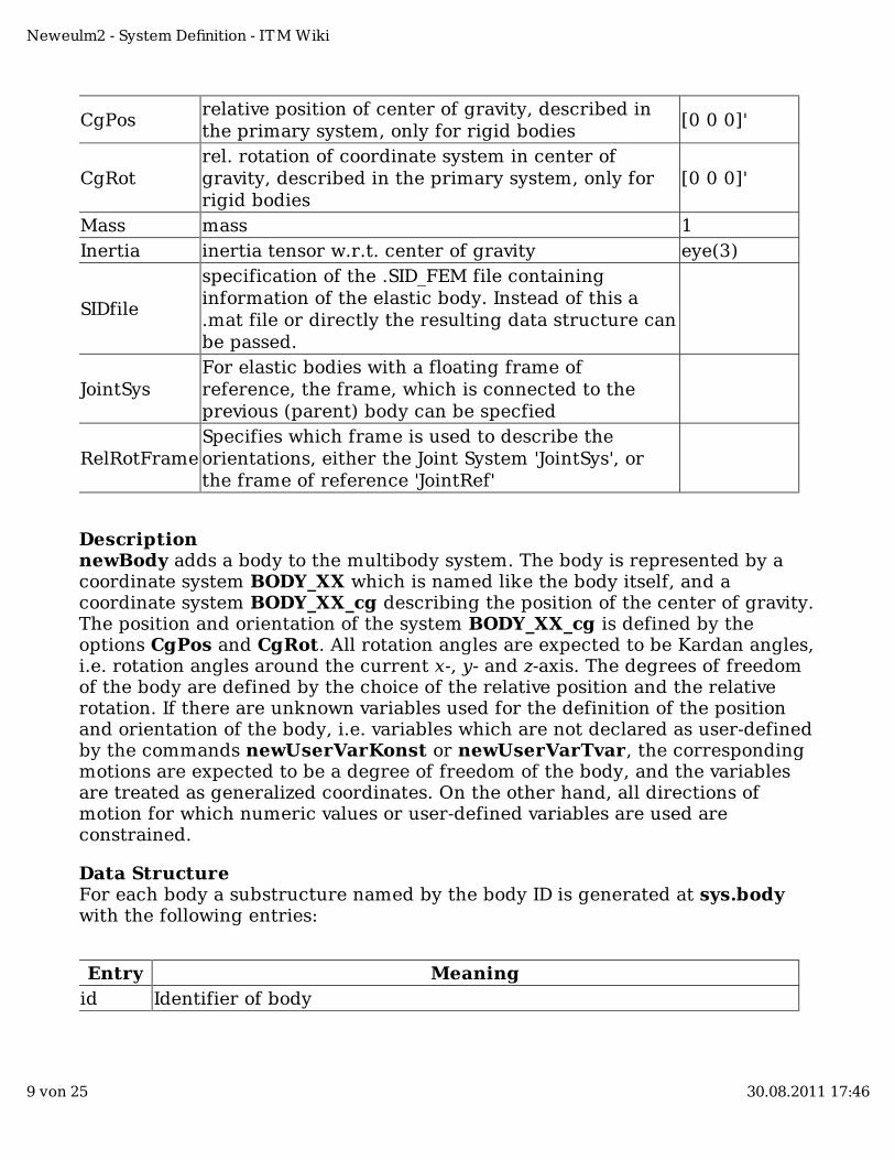
CgPosrelative position of center of gravity, described inthe primary system, only for rigid bodies
[0 0 0]'
CgRotrel. rotation of coordinate system in center ofgravity, described in the primary system, only forrigid bodies
[0 0 0]'
Mass mass 1Inertia inertia tensor w.r.t. center of gravity eye(3)
SIDfile
specification of the .SID_FEM file containinginformation of the elastic body. Instead of this a.mat file or directly the resulting data structure canbe passed.
JointSysFor elastic bodies with a floating frame ofreference, the frame, which is connected to theprevious (parent) body can be specfied
RelRotFrameSpecifies which frame is used to describe theorientations, either the Joint System 'JointSys', orthe frame of reference 'JointRef'
DescriptionnewBody adds a body to the multibody system. The body is represented by acoordinate system BODY_XX which is named like the body itself, and acoordinate system BODY_XX_cg describing the position of the center of gravity.The position and orientation of the system BODY_XX_cg is defined by theoptions CgPos and CgRot. All rotation angles are expected to be Kardan angles,i.e. rotation angles around the current x-, y- and z-axis. The degrees of freedomof the body are defined by the choice of the relative position and the relativerotation. If there are unknown variables used for the definition of the positionand orientation of the body, i.e. variables which are not declared as user-definedby the commands newUserVarKonst or newUserVarTvar, the correspondingmotions are expected to be a degree of freedom of the body, and the variablesare treated as generalized coordinates. On the other hand, all directions ofmotion for which numeric values or user-defined variables are used areconstrained.
Data StructureFor each body a substructure named by the body ID is generated at sys.bodywith the following entries:
Entry Meaningid Identifier of body
Neweulm2 - System Definition - ITM Wiki
9 von 25 30.08.2011 17:46
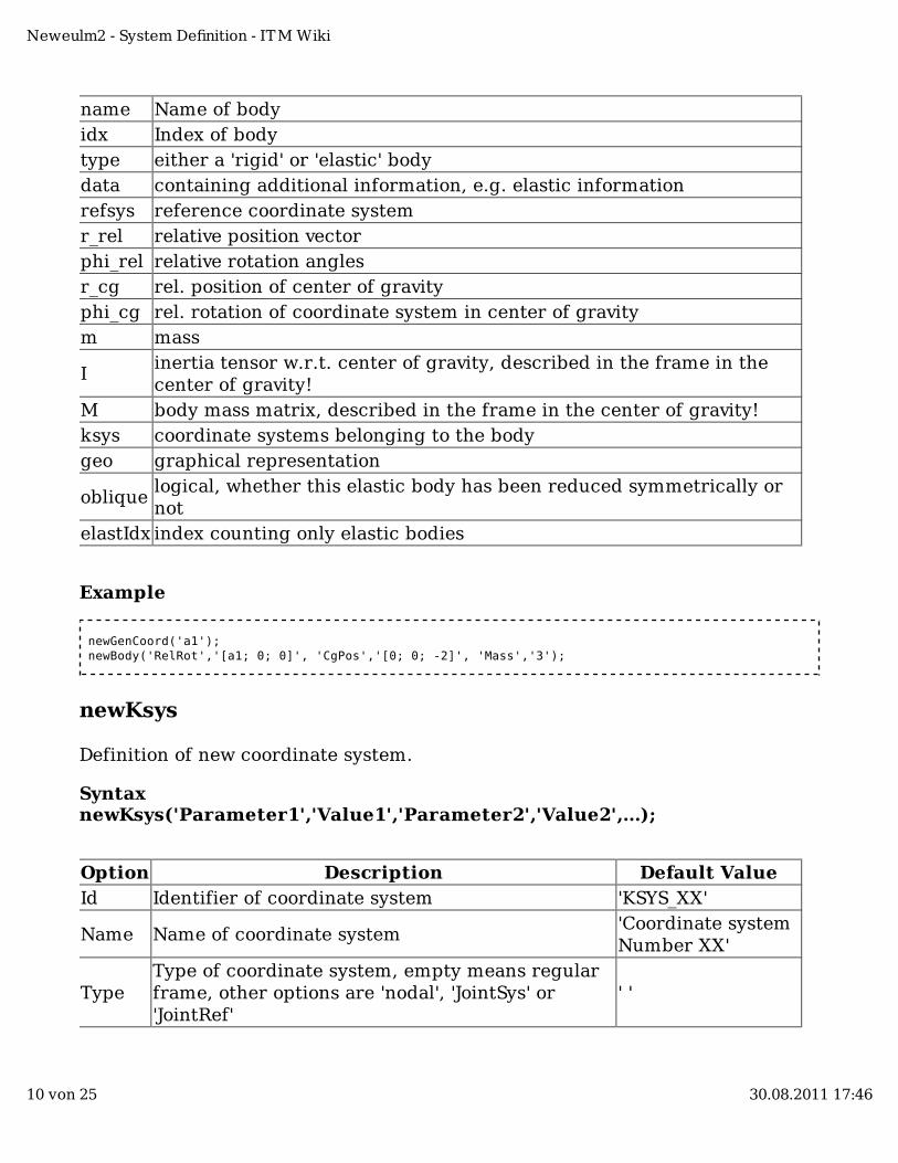
name Name of bodyidx Index of bodytype either a 'rigid' or 'elastic' bodydata containing additional information, e.g. elastic informationrefsys reference coordinate systemr_rel relative position vectorphi_rel relative rotation anglesr_cg rel. position of center of gravityphi_cg rel. rotation of coordinate system in center of gravitym mass
Iinertia tensor w.r.t. center of gravity, described in the frame in thecenter of gravity!
M body mass matrix, described in the frame in the center of gravity!ksys coordinate systems belonging to the bodygeo graphical representation
obliquelogical, whether this elastic body has been reduced symmetrically ornot
elastIdx index counting only elastic bodies
Example
newGenCoord('a1'); newBody('RelRot','[a1; 0; 0]', 'CgPos','[0; 0; -2]', 'Mass','3');
newKsys
Definition of new coordinate system.
SyntaxnewKsys('Parameter1','Value1','Parameter2','Value2',...);
Option Description Default ValueId Identifier of coordinate system 'KSYS_XX'
Name Name of coordinate system'Coordinate systemNumber XX'
TypeType of coordinate system, empty means regularframe, other options are 'nodal', 'JointSys' or'JointRef'
' '
Neweulm2 - System Definition - ITM Wiki
10 von 25 30.08.2011 17:46
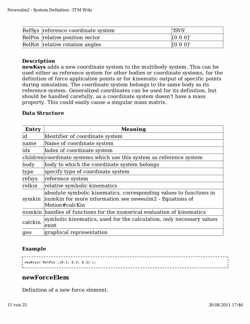
RefSys reference coordinate system 'ISYS'RelPos relative position vector [0 0 0]'RelRot relative rotation angles [0 0 0]'
DescriptionnewKsys adds a new coordinate system to the multibody system. This can beused either as reference system for other bodies or coordinate systems, for thedefinition of force application points or for kinematic output of specific pointsduring simulation. The coordinate system belongs to the same body as itsreference system. Generalized coordinates can be used for its definition, butshould be handled carefully, as a coordinate system doesn't have a massproperty. This could easily cause a singular mass matrix.
Data Structure
Entry Meaningid Identifier of coordinate systemname Name of coordinate systemidx Index of coordinate systemchildren coordinate systems which use this system as reference systembody body to which the coordinate system belongstype specify type of coordinate systemrefsys reference systemrelkin relative symbolic kinematics
symkinabsolute symbolic kinematics, corresponding values to functions innumkin for more information see neweulm2 - Equations ofMotion#calcKin
numkin handles of functions for the numerical evaluation of kinematics
calckinsymbolic kinematics, used for the calculation, only necessary valuesexist
geo graphical representation
Example
newKsys('RelPos',[0.1; 0.2; 0.3]');
newForceElem
Definition of a new force element.
Neweulm2 - System Definition - ITM Wiki
11 von 25 30.08.2011 17:46
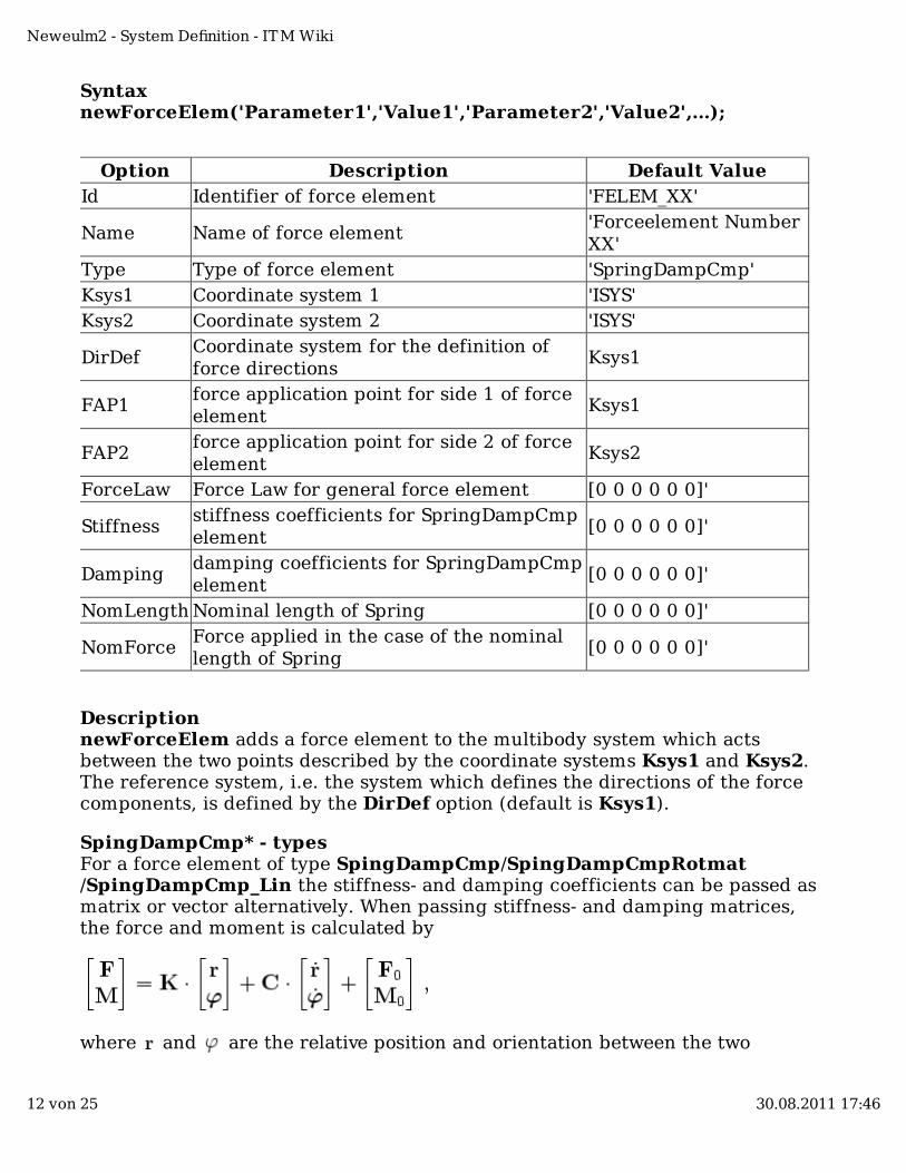
SyntaxnewForceElem('Parameter1','Value1','Parameter2','Value2',...);
Option Description Default ValueId Identifier of force element 'FELEM_XX'
Name Name of force element'Forceelement NumberXX'
Type Type of force element 'SpringDampCmp'Ksys1 Coordinate system 1 'ISYS'Ksys2 Coordinate system 2 'ISYS'
DirDefCoordinate system for the definition offorce directions
Ksys1
FAP1force application point for side 1 of forceelement
Ksys1
FAP2force application point for side 2 of forceelement
Ksys2
ForceLaw Force Law for general force element [0 0 0 0 0 0]'
Stiffnessstiffness coefficients for SpringDampCmpelement
[0 0 0 0 0 0]'
Dampingdamping coefficients for SpringDampCmpelement
[0 0 0 0 0 0]'
NomLength Nominal length of Spring [0 0 0 0 0 0]'
NomForceForce applied in the case of the nominallength of Spring
[0 0 0 0 0 0]'
DescriptionnewForceElem adds a force element to the multibody system which actsbetween the two points described by the coordinate systems Ksys1 and Ksys2.The reference system, i.e. the system which defines the directions of the forcecomponents, is defined by the DirDef option (default is Ksys1).
SpingDampCmp* - typesFor a force element of type SpingDampCmp/SpingDampCmpRotmat/SpingDampCmp_Lin the stiffness- and damping coefficients can be passed asmatrix or vector alternatively. When passing stiffness- and damping matrices,the force and moment is calculated by
where and are the relative position and orientation between the two
Neweulm2 - System Definition - ITM Wiki
12 von 25 30.08.2011 17:46
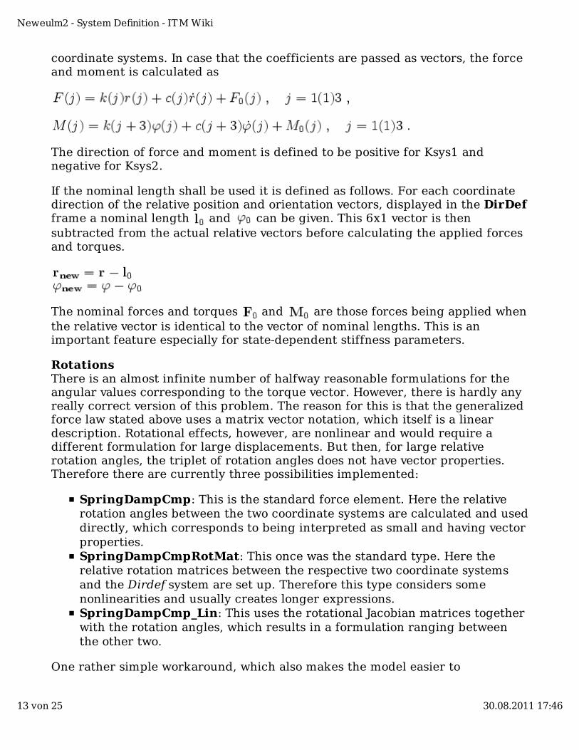
coordinate systems. In case that the coefficients are passed as vectors, the forceand moment is calculated as
The direction of force and moment is defined to be positive for Ksys1 andnegative for Ksys2.
If the nominal length shall be used it is defined as follows. For each coordinatedirection of the relative position and orientation vectors, displayed in the DirDefframe a nominal length and can be given. This 6x1 vector is thensubtracted from the actual relative vectors before calculating the applied forcesand torques.
The nominal forces and torques and are those forces being applied whenthe relative vector is identical to the vector of nominal lengths. This is animportant feature especially for state-dependent stiffness parameters.
RotationsThere is an almost infinite number of halfway reasonable formulations for theangular values corresponding to the torque vector. However, there is hardly anyreally correct version of this problem. The reason for this is that the generalizedforce law stated above uses a matrix vector notation, which itself is a lineardescription. Rotational effects, however, are nonlinear and would require adifferent formulation for large displacements. But then, for large relativerotation angles, the triplet of rotation angles does not have vector properties.Therefore there are currently three possibilities implemented:
SpringDampCmp: This is the standard force element. Here the relativerotation angles between the two coordinate systems are calculated and useddirectly, which corresponds to being interpreted as small and having vectorproperties.SpringDampCmpRotMat: This once was the standard type. Here therelative rotation matrices between the respective two coordinate systemsand the Dirdef system are set up. Therefore this type considers somenonlinearities and usually creates longer expressions.SpringDampCmp_Lin: This uses the rotational Jacobian matrices togetherwith the rotation angles, which results in a formulation ranging betweenthe other two.
One rather simple workaround, which also makes the model easier to
Neweulm2 - System Definition - ITM Wiki
13 von 25 30.08.2011 17:46
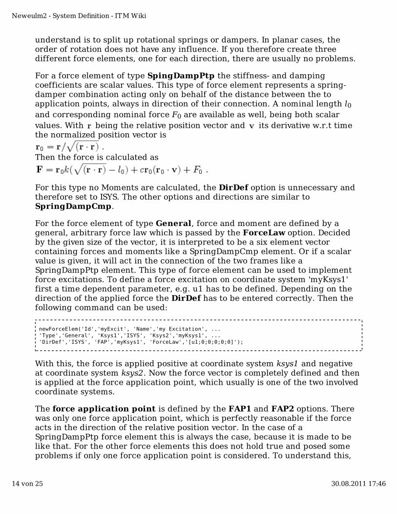
understand is to split up rotational springs or dampers. In planar cases, theorder of rotation does not have any influence. If you therefore create threedifferent force elements, one for each direction, there are usually no problems.
For a force element of type SpingDampPtp the stiffness- and dampingcoefficients are scalar values. This type of force element represents a spring-damper combination acting only on behalf of the distance between the toapplication points, always in direction of their connection. A nominal length l0and corresponding nominal force F0 are available as well, being both scalarvalues. With being the relative position vector and its derivative w.r.t timethe normalized position vector is
Then the force is calculated as
For this type no Moments are calculated, the DirDef option is unnecessary andtherefore set to ISYS. The other options and directions are similar toSpringDampCmp.
For the force element of type General, force and moment are defined by ageneral, arbitrary force law which is passed by the ForceLaw option. Decidedby the given size of the vector, it is interpreted to be a six element vectorcontaining forces and moments like a SpringDampCmp element. Or if a scalarvalue is given, it will act in the connection of the two frames like aSpringDampPtp element. This type of force element can be used to implementforce excitations. To define a force excitation on coordinate system 'myKsys1'first a time dependent parameter, e.g. u1 has to be defined. Depending on thedirection of the applied force the DirDef has to be entered correctly. Then thefollowing command can be used:
newForceElem('Id','myExcit', 'Name','my Excitation', ... 'Type','General', 'Ksys1','ISYS', 'Ksys2','myKsys1', ... 'DirDef','ISYS', 'FAP','myKsys1', 'ForceLaw','[u1;0;0;0;0;0]');
With this, the force is applied positive at coordinate system ksys1 and negativeat coordinate system ksys2. Now the force vector is completely defined and thenis applied at the force application point, which usually is one of the two involvedcoordinate systems.
The force application point is defined by the FAP1 and FAP2 options. Therewas only one force application point, which is perfectly reasonable if the forceacts in the direction of the relative position vector. In the case of aSpringDampPtp force element this is always the case, because it is made to belike that. For the other force elements this does not hold true and posed someproblems if only one force application point is considered. To understand this,
Neweulm2 - System Definition - ITM Wiki
14 von 25 30.08.2011 17:46
let's have a look at what the force application point is actually used for.
If a force is applied at a body in a way that its line of action does not passthrough the center of gravity, it will cause a moment. Let's consider aSpringDampCmp force element which connects two bodies. If its two coordinatesystems have a distance only in one coordinate direction, in which the forceelement will produce a force, everything works fine. If this displacement is, e.g.because of the choice of DirDef, to be separated in two coordinate directionswith a stiffness parameter each, the trouble begins as soon as these twoparameters are different. If the stiffness parameters are different, the force willno longer point into the direction of the relative position vector between the twocoordinate systems. Then it makes a difference which of the two coordinatesystems involved is used to calculate the moment, as they are no longerconnected by the line of action of the force. But the two coordinate systems haveto be on two different bodies for the force to appear in the equations of motion.Therefore for each of the involved bodies its respective coordinate system shouldbe considered as the force application point. On the other hand, one should beaware that such a force element may result in an unwanted moment withrespect to the center of gravity. But it is reasonable and in some case necessaryto use two different force application points. This effect could be easily avoidedby defining both force application points on the same coordinate system.
ATTENTION! Possible Source of Errors!
When using rotational springs there is a possibility of producing uncheckederrors. As long as possible, relative rotation angles between two coordinatesystems are set up using the relative angles of all coordinate systems inbetween. However, in some spatial cases this is not possible. Then the relativerotation angles will be extracted out of the relative rotation matrix. As soon as arotation matrix is involved, expressions like asin(sin(alpha)) will appear bystarting with the angle alpha, setting up the rotation matrix, causing asin(alpha) and attempting the inverse function. However, sometimes thesymbolic engine is unable to identify all of these expressions. The problem is,that basically asin(sin(alpha)) should be the same as alpha. However the range ofpossible values is different. The parameter alpha can take any real numberedvalue, asin(sin(alpha)) however is restricted to [-pi/2; pi/2]. This may cause somereally strange errors as they are very difficult to spot. The best way to avoidthem is to make sure that rotational springs and similar force elements alwaysuse angles inside the interval [-pi/2; pi/2], where there is no difference.
Data StructureFor each force element an entry in sys.felem with the ID of the force element iscreated. The data structure of a force element has the following entries:
Neweulm2 - System Definition - ITM Wiki
15 von 25 30.08.2011 17:46
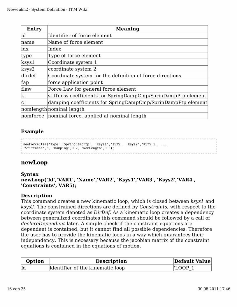
Entry Meaningid Identifier of force elementname Name of force elementidx Indextype Type of force elementksys1 Coordinate system 1ksys2 coordinate system 2dirdef Coordinate system for the definition of force directionsfap force application pointflaw Force Law for general force elementk stiffness coefficients for SpringDampCmp/SprinDampPtp elementc damping coefficients for SpringDampCmp/SprinDampPtp elementnomlength nominal lengthnomforce nominal force, applied at nominal length
Example
newForceElem('Type','SpringDampPtp', 'Ksys1','ISYS', 'Ksys2','KSYS_1', ... 'Stiffness',5, 'Damping',0.2, 'NomLength',0.3);
newLoop
SyntaxnewLoop('Id','VAR1', 'Name','VAR2', 'Ksys1','VAR3', 'Ksys2','VAR4','Constraints', VAR5);
DescriptionThis command creates a new kinematic loop, which is closed between ksys1 andksys2. The constrained directions are defined by Constraints, with respect to thecoordinate system denoted as DirDef. As a kinematic loop creates a dependencybetween generalized coordinates this command should be followed by a call ofdeclareDependent later. A simple check if the constraint equations aredependent is contained, but it cannot find all possible dependencies. Thereforethe user has to provide the kinematic loops in a way which guarantees theirindependency. This is necessary because the jacobian matrix of the constraintequations is contained in the equations of motion.
Option Description Default ValueId Identifier of the kinematic loop 'LOOP_1'
Neweulm2 - System Definition - ITM Wiki
16 von 25 30.08.2011 17:46
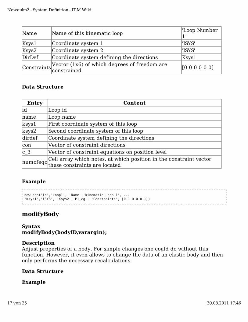
Name Name of this kinematic loop'Loop Number1'
Ksys1 Coordinate system 1 'ISYS'Ksys2 Coordinate system 2 'ISYS'DirDef Coordinate system defining the directions Ksys1
ConstraintsVector (1x6) of which degrees of freedom areconstrained
[0 0 0 0 0 0]
Data Structure
Entry Contentid Loop idname Loop nameksys1 First coordinate system of this loopksys2 Second coordinate system of this loopdirdef Coordinate system defining the directionscon Vector of constraint directionsc_3 Vector of constraint equations on position level
numofeqcCell array which notes, at which position in the constraint vectorthese constraints are located
Example
newLoop('Id','Loop1', 'Name','kinematic Loop 1', ... 'Ksys1','ISYS', 'Ksys2','P1_cg', 'Constraints', [0 1 0 0 0 1]);
modifyBody
SyntaxmodifyBody(bodyID,varargin);
DescriptionAdjust properties of a body. For simple changes one could do without thisfunction. However, it even allows to change the data of an elastic body and thenonly performs the necessary recalculations.
Data Structure
Example
Neweulm2 - System Definition - ITM Wiki
17 von 25 30.08.2011 17:46
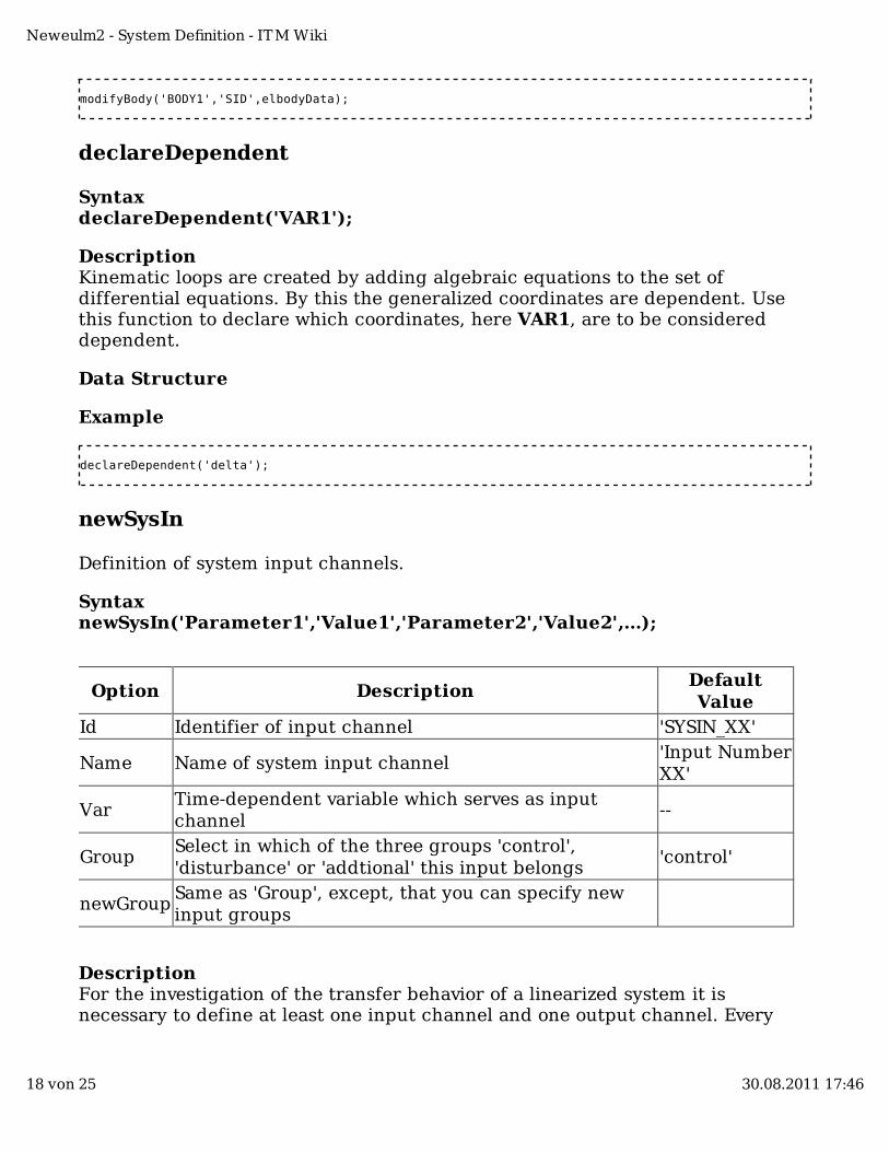
modifyBody('BODY1','SID',elbodyData);
declareDependent
SyntaxdeclareDependent('VAR1');
DescriptionKinematic loops are created by adding algebraic equations to the set ofdifferential equations. By this the generalized coordinates are dependent. Usethis function to declare which coordinates, here VAR1, are to be considereddependent.
Data Structure
Example
declareDependent('delta');
newSysIn
Definition of system input channels.
SyntaxnewSysIn('Parameter1','Value1','Parameter2','Value2',...);
Option DescriptionDefaultValue
Id Identifier of input channel 'SYSIN_XX'
Name Name of system input channel'Input NumberXX'
VarTime-dependent variable which serves as inputchannel
--
GroupSelect in which of the three groups 'control','disturbance' or 'addtional' this input belongs
'control'
newGroupSame as 'Group', except, that you can specify newinput groups
DescriptionFor the investigation of the transfer behavior of a linearized system it isnecessary to define at least one input channel and one output channel. Every
Neweulm2 - System Definition - ITM Wiki
18 von 25 30.08.2011 17:46
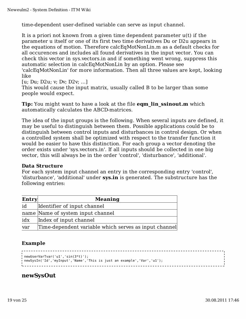
time-dependent user-defined variable can serve as input channel.
It is a priori not known from a given time dependent parameter u(t) if theparameter u itself or one of its first two time derivatives Du or D2u appears inthe equations of motion. Therefore calcEqMotNonLin.m as a default checks forall occurences and includes all found derivatives in the input vector. You cancheck this vector in sys.vectors.in and if something went wrong, suppress thisautomatic selection in calcEqMotNonLin by an option. Please see'calcEqMotNonLin' for more information. Then all three values are kept, lookinglike[u; Du; D2u; v; Dv; D2v; ...]This would cause the input matrix, usually called B to be larger than somepeople would expect.
Tip: You might want to have a look at the file eqm_lin_ssinout.m whichautomatically calculates the ABCD-matrices.
The idea of the input groups is the following. When several inputs are defined, itmay be useful to distinguish between them. Possible applications could be todistinguish between control inputs and disturbances in control design. Or whena controlled system shall be optimized with respect to the transfer function itwould be easier to have this distinction. For each group a vector denoting theorder exists under 'sys.vectors.in'. If all inputs should be collected in one bigvector, this will always be in the order 'control', 'disturbance', 'additional'.
Data StructureFor each system input channel an entry in the corresponding entry 'control','disturbance', 'additional' under sys.in is generated. The substructure has thefollowing entries:
Entry Meaningid Identifier of input channelname Name of system input channelidx Index of input channelvar Time-dependent variable which serves as input channel
Example
newUserVarTvar('u1','sin(3*t)'); newSysIn('Id','myInput','Name','This is just an example','Var','u1');
newSysOut
Neweulm2 - System Definition - ITM Wiki
19 von 25 30.08.2011 17:46
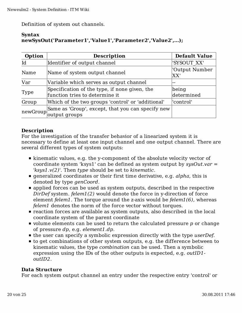
Definition of system out channels.
SyntaxnewSysOut('Parameter1','Value1','Parameter2','Value2',...);
Option Description Default ValueId Identifier of output channel 'SYSOUT_XX'
Name Name of system output channel'Output NumberXX'
Var Variable which serves as output channel --
TypeSpecification of the type, if none given, thefunction tries to determine it
beingdetermined
Group Which of the two groups 'control' or 'additional' 'control'
newGroupSame as 'Group', except, that you can specify newoutput groups
DescriptionFor the investigation of the transfer behavior of a linearized system it isnecessary to define at least one input channel and one output channel. There areseveral different types of system outputs:
kinematic values, e.g. the y-component of the absolute velocity vector ofcoordinate system 'ksys1' can be defined as system output by sysOut.var ='ksys1.v(2)'. Then type should be set to kinematic.generalized coordinates or their first time derivative, e.g. alpha, this isdenoted by type genCoord.applied forces can be used as system outputs, described in the respectiveDirDef system. felem1(2) would denote the force in y-direction of forceelement felem1. The torque around the z-axis would be felem1(6), whereasfelem1 denotes the norm of the force vector without torques.reaction forces are available as system outputs, also described in the localcoordinate system of the parent coordinatevolume elements can be used to return the calculated pressure p or changeof pressure dp, e.g. element1.dp.the user can specify a symbolic expression directly with the type userDef.to get combinations of other system outputs, e.g. the difference between tokinematic values, the type combination can be used. Then a symbolicexpression using the IDs of the other outputs is expected, e.g. outID1-outID2.
Data StructureFor each system output channel an entry under the respective entry 'control' or
Neweulm2 - System Definition - ITM Wiki
20 von 25 30.08.2011 17:46
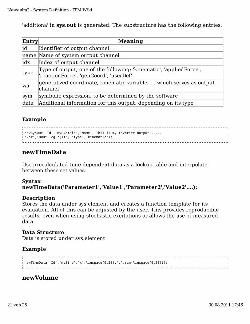
'additiona' in sys.out is generated. The substructure has the following entries:
Entry Meaningid Identifier of output channelname Name of system output channelidx Index of output channel
typeType of output, one of the following: 'kinematic', 'appliedForce','reactionForce', 'genCoord', 'userDef'
vargeneralized coordinate, kinematic variable, ... which serves as outputchannel
sym symbolic expression, to be determined by the softwaredata Additional information for this output, depending on its type
Example
newSysOut('Id','myExample','Name','This is my favorite output', ... 'Var','BODY1_cg.r(1)', 'Type','kinematic');
newTimeData
Use precalculated time dependent data as a lookup table and interpolatebetween these set values.
SyntaxnewTimeData('Parameter1','Value1','Parameter2','Value2',...);
DescriptionStores the data under sys.element and creates a function template for itsevaluation. All of this can be adjusted by the user. This provides reproducibleresults, even when using stochastic excitations or allows the use of measureddata.
Data StructureData is stored under sys.element
Example
newTimeData('Id','mySine','x',linspace(0,20),'y',sin(linspace(0,20)));
newVolume
Neweulm2 - System Definition - ITM Wiki
21 von 25 30.08.2011 17:46
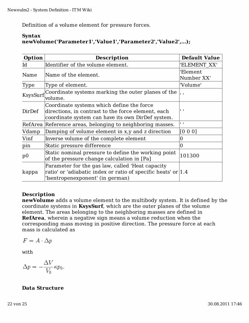
Definition of a volume element for pressure forces.
SyntaxnewVolume('Parameter1','Value1','Parameter2','Value2',...);
Option Description Default ValueId Identifier of the volume element. 'ELEMENT_XX'
Name Name of the element.'ElementNumber XX'
Type Type of element. 'Volume'
KsysSurfCoordinate systems marking the outer planes of thevolume.
' '
DirDefCoordinate systems which define the forcedirections, in contrast to the force element, eachcoordinate system can have its own DirDef system.
' '
RefArea Reference areas, belonging to neighboring masses. ' 'Vdamp Damping of volume element in x,y and z direction [0 0 0]Vinf Inverse volume of the complete element 0pin Static pressure difference 0
p0Static nominal pressure to define the working pointof the pressure change calculation in [Pa]
101300
kappaParameter for the gas law, called 'Heat capacityratio' or 'adiabatic index or ratio of specific heats' or'Isentropenexponent' (in german)
1.4
DescriptionnewVolume adds a volume element to the multibody system. It is defined by thecoordinate systems in KsysSurf, which are the outer planes of the volumeelement. The areas belonging to the neighboring masses are defined inRefArea, wherein a negative sign means a volume reduction when thecorresponding mass moving in positive direction. The pressure force at eachmass is calculated as
with
Data Structure
Neweulm2 - System Definition - ITM Wiki
22 von 25 30.08.2011 17:46
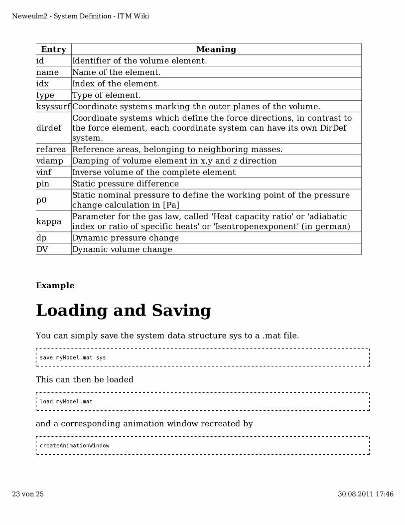
Entry Meaningid Identifier of the volume element.name Name of the element.idx Index of the element.type Type of element.ksyssurf Coordinate systems marking the outer planes of the volume.
dirdefCoordinate systems which define the force directions, in contrast tothe force element, each coordinate system can have its own DirDefsystem.
refarea Reference areas, belonging to neighboring masses.vdamp Damping of volume element in x,y and z directionvinf Inverse volume of the complete elementpin Static pressure difference
p0Static nominal pressure to define the working point of the pressurechange calculation in [Pa]
kappaParameter for the gas law, called 'Heat capacity ratio' or 'adiabaticindex or ratio of specific heats' or 'Isentropenexponent' (in german)
dp Dynamic pressure changeDV Dynamic volume change
Example
Loading and SavingYou can simply save the system data structure sys to a .mat file.
save myModel.mat sys
This can then be loaded
load myModel.mat
and a corresponding animation window recreated by
createAnimationWindow
Neweulm2 - System Definition - ITM Wiki
23 von 25 30.08.2011 17:46
load_neweulm2_System
Syntaxload_neweulm2_System(filename, filepath, CallMode_);
DescriptionAs a difference to simply saving the system data structure, the figure andsettings of the graphical user interface (if available) are stored. Then theanimation window will look exactly the same and not just almost.
All of these arguments are optional. A filename and its path (filepath) can bepassed to the function. If they are ommitted the standard dialog to select a filefor loading is opened. The parameter CallMode_ can be used if the function shallbe called from the command line. As a default the structure gui and theuser-interface neweulm2 are adjusted. For more information type helpload_neweulm2_System. This function was created to be called from the GUI, butis also available for the batch mode.
Example
load_neweulm2_System;load_neweulm2_System('mysystem.mat');
save_neweulm2_System
Syntaxsave_neweulm2_System(filename,filepath,IncludeResults_);
DescriptionAll of these arguments are optional. This function allows the user to save asystem and its corresponding figure if available. The file will be called filenameand located in the folder filepath. With the boolean parameter IncludeResults_the user can decide if simulation results shall be included in the saved file. If thefilename is not specified, the standard dialog box to save files will be openedwhere the user can enter a filename. This function was created to be called fromthe GUI, but is also available for the batch mode.
Example
save_neweulm2_System;
See also
Neweulm2 - System Definition - ITM Wiki
24 von 25 30.08.2011 17:46
ITM Wiki
neweulm2neweulm2#Function reference
neweulm2 - Equations of Motionneweulm2 - Simulation and Animationneweulm2 - Exporting
Retrieved from "http://www.itm.uni-stuttgart.de/itmwiki/index.php/Neweulm2_-_System_Definition"
This page was last modified 14:51, 30 August 2011.
Neweulm2 - System Definition - ITM Wiki
25 von 25 30.08.2011 17:46
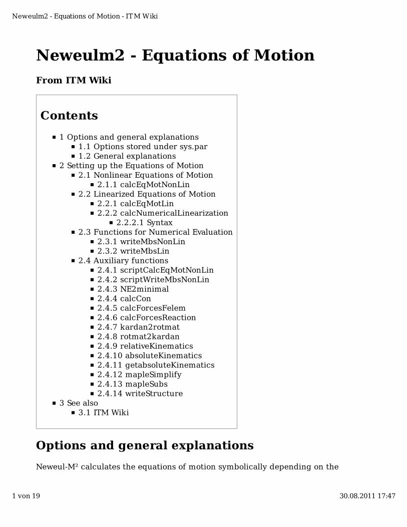
Neweulm2 - Equations of Motion
From ITM Wiki
Contents
1 Options and general explanations1.1 Options stored under sys.par1.2 General explanations
2 Setting up the Equations of Motion2.1 Nonlinear Equations of Motion
2.1.1 calcEqMotNonLin2.2 Linearized Equations of Motion
2.2.1 calcEqMotLin2.2.2 calcNumericalLinearization
2.2.2.1 Syntax2.3 Functions for Numerical Evaluation
2.3.1 writeMbsNonLin2.3.2 writeMbsLin
2.4 Auxiliary functions2.4.1 scriptCalcEqMotNonLin2.4.2 scriptWriteMbsNonLin2.4.3 NE2minimal2.4.4 calcCon2.4.5 calcForcesFelem2.4.6 calcForcesReaction2.4.7 kardan2rotmat2.4.8 rotmat2kardan2.4.9 relativeKinematics2.4.10 absoluteKinematics2.4.11 getabsoluteKinematics2.4.12 mapleSimplify2.4.13 mapleSubs2.4.14 writeStructure
3 See also3.1 ITM Wiki
Options and general explanations
Neweul-M² calculates the equations of motion symbolically depending on the
Neweulm2 - Equations of Motion - ITM Wiki
1 von 19 30.08.2011 17:47
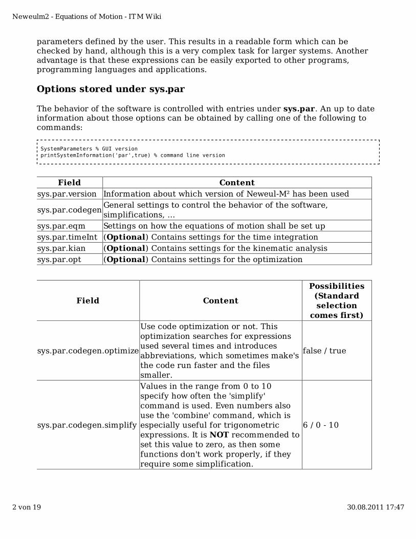
parameters defined by the user. This results in a readable form which can bechecked by hand, although this is a very complex task for larger systems. Anotheradvantage is that these expressions can be easily exported to other programs,programming languages and applications.
Options stored under sys.par
The behavior of the software is controlled with entries under sys.par. An up to dateinformation about those options can be obtained by calling one of the following tocommands:
SystemParameters % GUI version printSystemInformation('par',true) % command line version
Field Contentsys.par.version Information about which version of Neweul-M² has been used
sys.par.codegenGeneral settings to control the behavior of the software,simplifications, ...
sys.par.eqm Settings on how the equations of motion shall be set upsys.par.timeInt (Optional) Contains settings for the time integrationsys.par.kian (Optional) Contains settings for the kinematic analysissys.par.opt (Optional) Contains settings for the optimization
Field Content
Possibilities(Standardselection
comes first)
sys.par.codegen.optimize
Use code optimization or not. Thisoptimization searches for expressionsused several times and introducesabbreviations, which sometimes make'sthe code run faster and the filessmaller.
false / true
sys.par.codegen.simplify
Values in the range from 0 to 10specify how often the 'simplify'command is used. Even numbers alsouse the 'combine' command, which isespecially useful for trigonometricexpressions. It is NOT recommended toset this value to zero, as then somefunctions don't work properly, if theyrequire some simplification.
6 / 0 - 10
Neweulm2 - Equations of Motion - ITM Wiki
2 von 19 30.08.2011 17:47
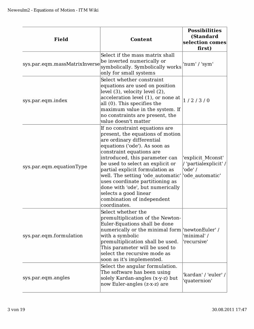
Field Content
Possibilities(Standard
selection comesfirst)
sys.par.eqm.massMatrixInverse
Select if the mass matrix shallbe inverted numerically orsymbolically. Symbolically worksonly for small systems
'num' / 'sym'
sys.par.eqm.index
Select whether constraintequations are used on positionlevel (3), velocity level (2),acceleration level (1), or none atall (0). This specifies themaximum value in the system. Ifno constraints are present, thevalue doesn't matter
1 / 2 / 3 / 0
sys.par.eqm.equationType
If no constraint equations arepresent, the equations of motionare ordinary differentialequations ('ode'). As soon asconstraint equations areintroduced, this parameter canbe used to select an explicit orpartial explicit formulation aswell. The setting 'ode_automatic'uses coordinate partitioning asdone with 'ode', but numericallyselects a good linearcombination of independentcoordinates.
'explicit_Mconst'/ 'partialexplicit' /'ode' /'ode_automatic'
sys.par.eqm.formulation
Select whether thepremultiplication of the Newton-Euler-Equations shall be donenumerically or the minimal formwith a symbolicpremultiplication shall be used.This parameter will be used toselect the recursive mode assoon as it's implemented.
'newtonEuler' /'minimal' /'recursive'
sys.par.eqm.angles
Select the angular formulation.The software has been usingsolely Kardan-angles (x-y-z) butnow Euler-angles (z-x-z) are
'kardan' / 'euler' /'quaternion'
Neweulm2 - Equations of Motion - ITM Wiki
3 von 19 30.08.2011 17:47
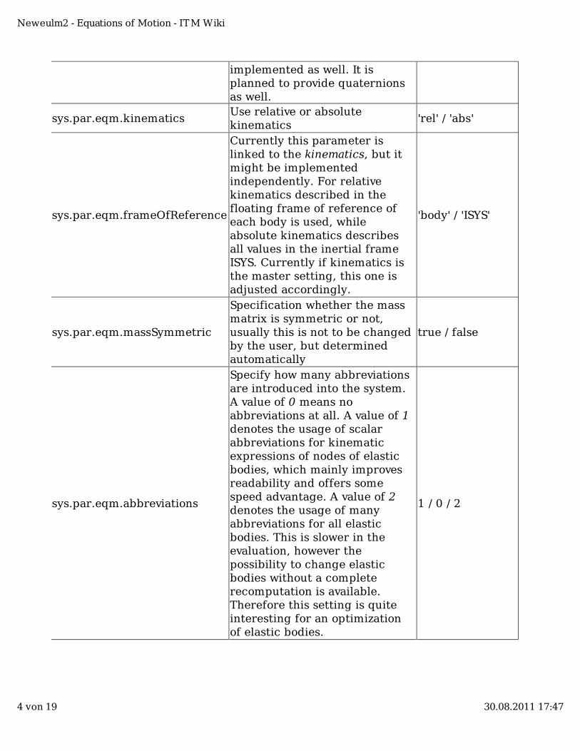
implemented as well. It isplanned to provide quaternionsas well.
sys.par.eqm.kinematicsUse relative or absolutekinematics
'rel' / 'abs'
sys.par.eqm.frameOfReference
Currently this parameter islinked to the kinematics, but itmight be implementedindependently. For relativekinematics described in thefloating frame of reference ofeach body is used, whileabsolute kinematics describesall values in the inertial frameISYS. Currently if kinematics isthe master setting, this one isadjusted accordingly.
'body' / 'ISYS'
sys.par.eqm.massSymmetric
Specification whether the massmatrix is symmetric or not,usually this is not to be changedby the user, but determinedautomatically
true / false
sys.par.eqm.abbreviations
Specify how many abbreviationsare introduced into the system.A value of 0 means noabbreviations at all. A value of 1denotes the usage of scalarabbreviations for kinematicexpressions of nodes of elasticbodies, which mainly improvesreadability and offers somespeed advantage. A value of 2denotes the usage of manyabbreviations for all elasticbodies. This is slower in theevaluation, however thepossibility to change elasticbodies without a completerecomputation is available.Therefore this setting is quiteinteresting for an optimizationof elastic bodies.
1 / 0 / 2
Neweulm2 - Equations of Motion - ITM Wiki
4 von 19 30.08.2011 17:47
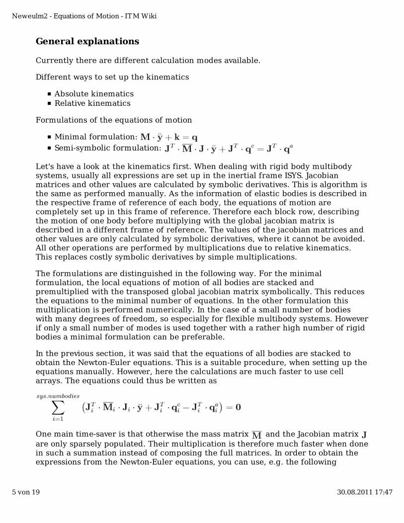
General explanations
Currently there are different calculation modes available.
Different ways to set up the kinematics
Absolute kinematicsRelative kinematics
Formulations of the equations of motion
Minimal formulation:
Semi-symbolic formulation:
Let's have a look at the kinematics first. When dealing with rigid body multibodysystems, usually all expressions are set up in the inertial frame ISYS. Jacobianmatrices and other values are calculated by symbolic derivatives. This is algorithm isthe same as performed manually. As the information of elastic bodies is described inthe respective frame of reference of each body, the equations of motion arecompletely set up in this frame of reference. Therefore each block row, describingthe motion of one body before multiplying with the global jacobian matrix isdescribed in a different frame of reference. The values of the jacobian matrices andother values are only calculated by symbolic derivatives, where it cannot be avoided.All other operations are performed by multiplications due to relative kinematics.This replaces costly symbolic derivatives by simple multiplications.
The formulations are distinguished in the following way. For the minimalformulation, the local equations of motion of all bodies are stacked andpremultiplied with the transposed global jacobian matrix symbolically. This reducesthe equations to the minimal number of equations. In the other formulation thismultiplication is performed numerically. In the case of a small number of bodieswith many degrees of freedom, so especially for flexible multibody systems. Howeverif only a small number of modes is used together with a rather high number of rigidbodies a minimal formulation can be preferable.
In the previous section, it was said that the equations of all bodies are stacked toobtain the Newton-Euler equations. This is a suitable procedure, when setting up theequations manually. However, here the calculations are much faster to use cellarrays. The equations could thus be written as
One main time-saver is that otherwise the mass matrix and the Jacobian matrix are only sparsely populated. Their multiplication is therefore much faster when donein such a summation instead of composing the full matrices. In order to obtain theexpressions from the Newton-Euler equations, you can use, e.g. the following
Neweulm2 - Equations of Motion - ITM Wiki
5 von 19 30.08.2011 17:47
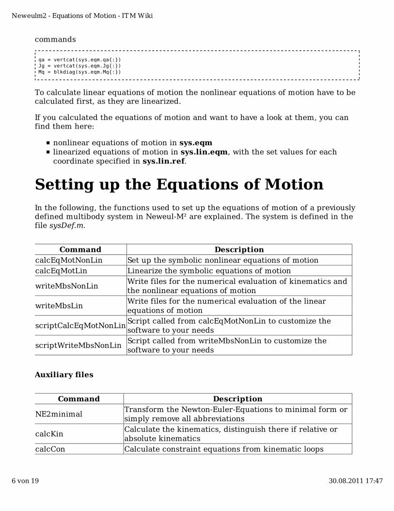
commands
qa = vertcat(sys.eqm.qa{:}) Jg = vertcat(sys.eqm.Jg{:}) Mq = blkdiag(sys.eqm.Mq{:})
To calculate linear equations of motion the nonlinear equations of motion have to becalculated first, as they are linearized.
If you calculated the equations of motion and want to have a look at them, you canfind them here:
nonlinear equations of motion in sys.eqmlinearized equations of motion in sys.lin.eqm, with the set values for eachcoordinate specified in sys.lin.ref.
Setting up the Equations of MotionIn the following, the functions used to set up the equations of motion of a previouslydefined multibody system in Neweul-M² are explained. The system is defined in thefile sysDef.m.
Command DescriptioncalcEqMotNonLin Set up the symbolic nonlinear equations of motioncalcEqMotLin Linearize the symbolic equations of motion
writeMbsNonLinWrite files for the numerical evaluation of kinematics andthe nonlinear equations of motion
writeMbsLinWrite files for the numerical evaluation of the linearequations of motion
scriptCalcEqMotNonLinScript called from calcEqMotNonLin to customize thesoftware to your needs
scriptWriteMbsNonLinScript called from writeMbsNonLin to customize thesoftware to your needs
Auxiliary files
Command Description
NE2minimalTransform the Newton-Euler-Equations to minimal form orsimply remove all abbreviations
calcKinCalculate the kinematics, distinguish there if relative orabsolute kinematics
calcCon Calculate constraint equations from kinematic loops
Neweulm2 - Equations of Motion - ITM Wiki
6 von 19 30.08.2011 17:47
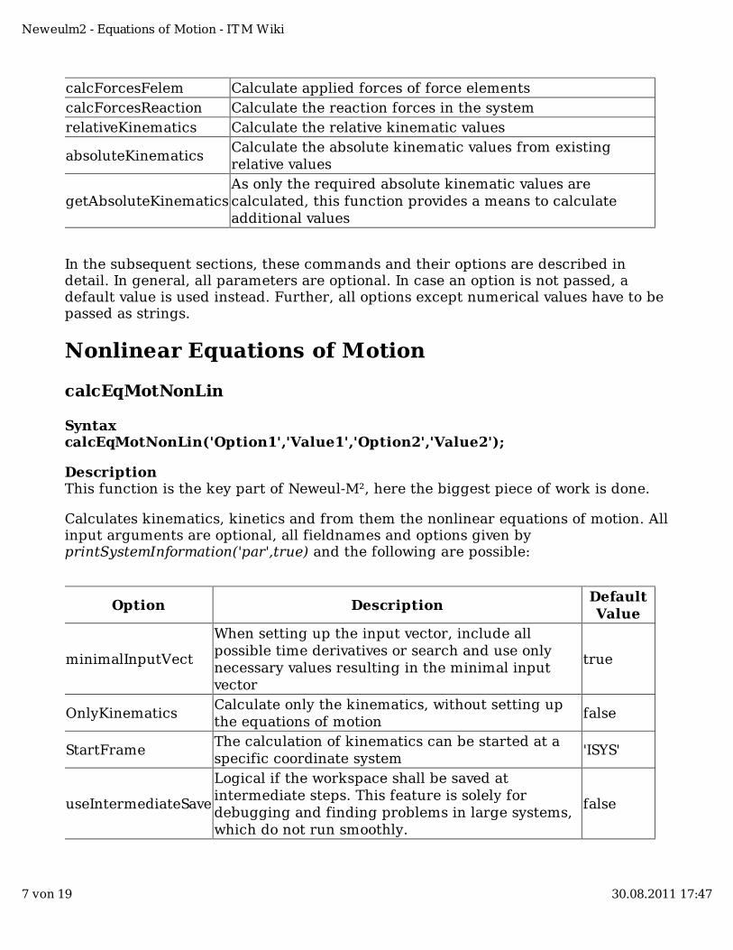
calcForcesFelem Calculate applied forces of force elementscalcForcesReaction Calculate the reaction forces in the systemrelativeKinematics Calculate the relative kinematic values
absoluteKinematicsCalculate the absolute kinematic values from existingrelative values
getAbsoluteKinematicsAs only the required absolute kinematic values arecalculated, this function provides a means to calculateadditional values
In the subsequent sections, these commands and their options are described indetail. In general, all parameters are optional. In case an option is not passed, adefault value is used instead. Further, all options except numerical values have to bepassed as strings.
Nonlinear Equations of Motion
calcEqMotNonLin
SyntaxcalcEqMotNonLin('Option1','Value1','Option2','Value2');
DescriptionThis function is the key part of Neweul-M², here the biggest piece of work is done.
Calculates kinematics, kinetics and from them the nonlinear equations of motion. Allinput arguments are optional, all fieldnames and options given byprintSystemInformation('par',true) and the following are possible:
Option DescriptionDefaultValue
minimalInputVect
When setting up the input vector, include allpossible time derivatives or search and use onlynecessary values resulting in the minimal inputvector
true
OnlyKinematicsCalculate only the kinematics, without setting upthe equations of motion
false
StartFrameThe calculation of kinematics can be started at aspecific coordinate system
'ISYS'
useIntermediateSave
Logical if the workspace shall be saved atintermediate steps. This feature is solely fordebugging and finding problems in large systems,which do not run smoothly.
false
Neweulm2 - Equations of Motion - ITM Wiki
7 von 19 30.08.2011 17:47
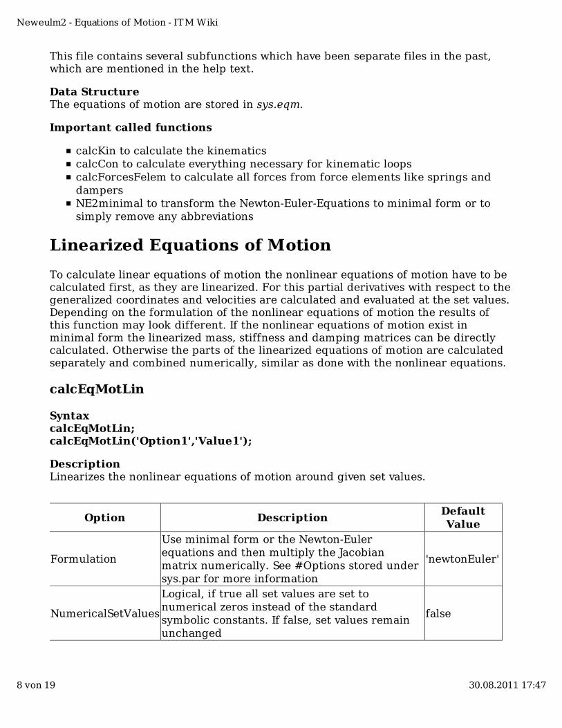
This file contains several subfunctions which have been separate files in the past,which are mentioned in the help text.
Data StructureThe equations of motion are stored in sys.eqm.
Important called functions
calcKin to calculate the kinematicscalcCon to calculate everything necessary for kinematic loopscalcForcesFelem to calculate all forces from force elements like springs anddampersNE2minimal to transform the Newton-Euler-Equations to minimal form or tosimply remove any abbreviations
Linearized Equations of Motion
To calculate linear equations of motion the nonlinear equations of motion have to becalculated first, as they are linearized. For this partial derivatives with respect to thegeneralized coordinates and velocities are calculated and evaluated at the set values.Depending on the formulation of the nonlinear equations of motion the results ofthis function may look different. If the nonlinear equations of motion exist inminimal form the linearized mass, stiffness and damping matrices can be directlycalculated. Otherwise the parts of the linearized equations of motion are calculatedseparately and combined numerically, similar as done with the nonlinear equations.
calcEqMotLin
SyntaxcalcEqMotLin;calcEqMotLin('Option1','Value1');
DescriptionLinearizes the nonlinear equations of motion around given set values.
Option DescriptionDefaultValue
Formulation
Use minimal form or the Newton-Eulerequations and then multiply the Jacobianmatrix numerically. See #Options stored undersys.par for more information
'newtonEuler'
NumericalSetValues
Logical, if true all set values are set tonumerical zeros instead of the standardsymbolic constants. If false, set values remainunchanged
false
Neweulm2 - Equations of Motion - ITM Wiki
8 von 19 30.08.2011 17:47
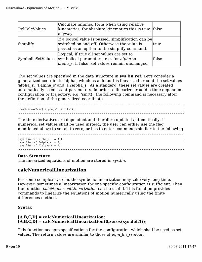
RelCalcValuesCalculate minimal form when using relativekinematics, for absolute kinematics this is trueanyway
false
SimplifyIf a logical value is passed, simplification can beswitched on and off. Otherwise the value ispassed as an option to the simplify command.
true
SymbolicSetValuesLogical, if true all set values are set tosymbolical parameters, e.g. for alpha toalpha_s. If false, set values remain unchanged
false
The set values are specified in the data structure in sys.lin.ref. Let's consider ageneralized coordinate 'alpha', which as a default is linearized around the set values'alpha_s', 'Dalpha_s' and 'D2alpha_s'. As a standard, these set values are createdautomatically as constant parameters. In order to linearize around a time dependentconfiguration or trajectory, e.g. 'sin(t)', the following command is necessary afterthe definition of the generalized coordinate
newUserVarTvar('alpha_s','sin(t)');
The time derivatives are dependent and therefore updated automatically. Ifnumerical set values shall be used instead, the user can either use the flagmentioned above to set all to zero, or has to enter commands similar to the following
sys.lin.ref.alpha_s = 0.1; sys.lin.ref.Dalpha_s = 0; sys.lin.ref.D2alpha_s = 0;
Data StructureThe linearized equations of motion are stored in sys.lin.
calcNumericalLinearization
For some complex systems the symbolic linearization may take very long time.However, sometimes a linearization for one specific configuration is sufficient. Thenthe function calcNumericalLinearization can be useful. This function providescommands to linearize the equations of motion numerically using the finitedifferences method.
Syntax
[A,B,C,D] = calcNumericalLinearization;[A,B,C,D] = calcNumericalLinearization(0,zeros(sys.dof,1));
This function accepts specifications for the configuration which shall be used as setvalues. The return values are similar to those of eqm_lin_ssinout.
Neweulm2 - Equations of Motion - ITM Wiki
9 von 19 30.08.2011 17:47
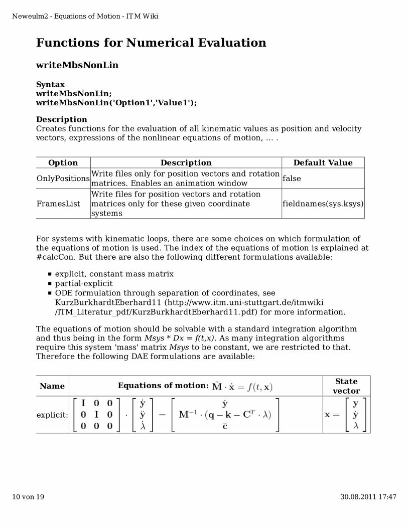
Functions for Numerical Evaluation
writeMbsNonLin
SyntaxwriteMbsNonLin;writeMbsNonLin('Option1','Value1');
DescriptionCreates functions for the evaluation of all kinematic values as position and velocityvectors, expressions of the nonlinear equations of motion, ... .
Option Description Default Value
OnlyPositionsWrite files only for position vectors and rotationmatrices. Enables an animation window
false
FramesListWrite files for position vectors and rotationmatrices only for these given coordinatesystems
fieldnames(sys.ksys)
For systems with kinematic loops, there are some choices on which formulation ofthe equations of motion is used. The index of the equations of motion is explained at#calcCon. But there are also the following different formulations available:
explicit, constant mass matrixpartial-explicitODE formulation through separation of coordinates, seeKurzBurkhardtEberhard11 (http://www.itm.uni-stuttgart.de/itmwiki/ITM_Literatur_pdf/KurzBurkhardtEberhard11.pdf) for more information.
The equations of motion should be solvable with a standard integration algorithmand thus being in the form Msys * Dx = f(t,x). As many integration algorithmsrequire this system 'mass' matrix Msys to be constant, we are restricted to that.Therefore the following DAE formulations are available:
Name Equations of motion: Statevector
explicit:
Neweulm2 - Equations of Motion - ITM Wiki
10 von 19 30.08.2011 17:47
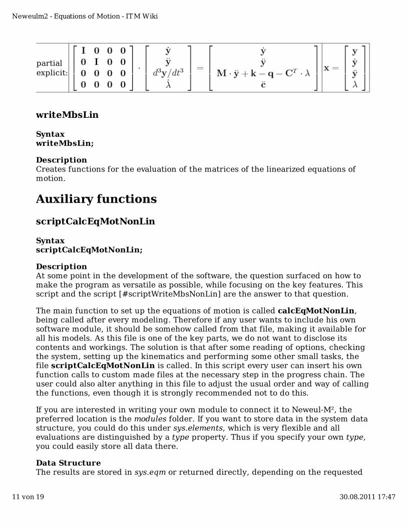
partialexplicit:
writeMbsLin
SyntaxwriteMbsLin;
DescriptionCreates functions for the evaluation of the matrices of the linearized equations ofmotion.
Auxiliary functions
scriptCalcEqMotNonLin
SyntaxscriptCalcEqMotNonLin;
DescriptionAt some point in the development of the software, the question surfaced on how tomake the program as versatile as possible, while focusing on the key features. Thisscript and the script [#scriptWriteMbsNonLin] are the answer to that question.
The main function to set up the equations of motion is called calcEqMotNonLin,being called after every modeling. Therefore if any user wants to include his ownsoftware module, it should be somehow called from that file, making it available forall his models. As this file is one of the key parts, we do not want to disclose itscontents and workings. The solution is that after some reading of options, checkingthe system, setting up the kinematics and performing some other small tasks, thefile scriptCalcEqMotNonLin is called. In this script every user can insert his ownfunction calls to custom made files at the necessary step in the progress chain. Theuser could also alter anything in this file to adjust the usual order and way of callingthe functions, even though it is strongly recommended not to do this.
If you are interested in writing your own module to connect it to Neweul-M², thepreferred location is the modules folder. If you want to store data in the system datastructure, you could do this under sys.elements, which is very flexible and allevaluations are distinguished by a type property. Thus if you specify your own type,you could easily store all data there.
Data StructureThe results are stored in sys.eqm or returned directly, depending on the requested
Neweulm2 - Equations of Motion - ITM Wiki
11 von 19 30.08.2011 17:47
evaluations.
scriptWriteMbsNonLin
SyntaxscriptWriteMbsNonLin;
DescriptionSimilar to scriptCalcEqMotNonLin, this script is called from writeMbsNonLin,which is the main function to write files after the equations have been set up. Pleasefeel free to insert your own calls.
Data StructureNo entry
NE2minimal
Syntaxresult = NE2minimal(varargin);
DescriptionThis functio started as a nice way to obtain the minimal formulation if the Newton-Euler-Equations have already been set up. As the expressions of the equations ofmotion may contain non-scalar abbreviations, which then alter the dimensions visiblefor the user, this function provides additional functionality. It can remove allabbreviations, which is partly necessary for the minimal form and completelynecessary for the symbolic linearization of the equations of motion. However, thisfunction can also provide the expressions of the Newton-Euler-Equations as symbolicmatrices and not as cell arrays as stored under sys.eqm. For any options on how tocall the function to obtain the result you need, please have a look at the helpmessage of this file.
Data StructureThe results are stored in sys.eqm or returned directly, depending on the requestedevaluations.
calcCon
SyntaxcalcCon(y,Dy,D2y);
DescriptionCalculates the constraint equations for kinematic loops. The subfunction 'comcon'checks for redundant constraint equations and tries to assure their independency. Itdoes not cover all cases, so the user has some responsibility to define independentconstraints. The subfunction 'con2loop' assigns the constraint equations to the loops.
Neweulm2 - Equations of Motion - ITM Wiki
12 von 19 30.08.2011 17:47
There is a parameter under sys.par.eqm.constraints.index which specifies the indexof the system of equations. If this index is set to 1, the constraint equations are usedon acceleration level, for 2 on velocity and for 3 on position level. However, the userhas to ensure that the integration algorithm can handle the selected constraints.This function only calculates the necessary derivatives of the constraint equationsand will skip the remaining part. Under #writeMbsNonLin the parameterformulation is described, which is closely related to the index.
Data StructureThe results are stored in sys.eqc.
Contained subfunctions
comconcon2loop
calcForcesFelem
Syntax[qa, felemStruct_, Data_] = calcForcesFelem(varargin);
DescriptionCalculates all forces from force elements like spring-damper combinations, i.e.everything stored under sys.felem. If nothing is specified, this function does exactlythat. However, the user may explicitly give a structure of force elements, then this isused and only the contained force elements are considered for the force calculation.
Data StructureEntries have to be made by the user to the system data structure, so it is moreversatile.
Example
calcForcesFelem;
calcForcesReaction
Syntax[qr, allRfelem] = calcForcesReaction(varargin);
DescriptionCalculate the necessary values for the evaluation of reaction forces. Depending onthe options specified, the reaction forces are calculated symbolically in therespective frame of reference, or they are only calculated as in the Newton-Euler-equations and further evaluations are done numerically.
Input parameters, all optional and pairwise, are
Neweulm2 - Equations of Motion - ITM Wiki
13 von 19 30.08.2011 17:47
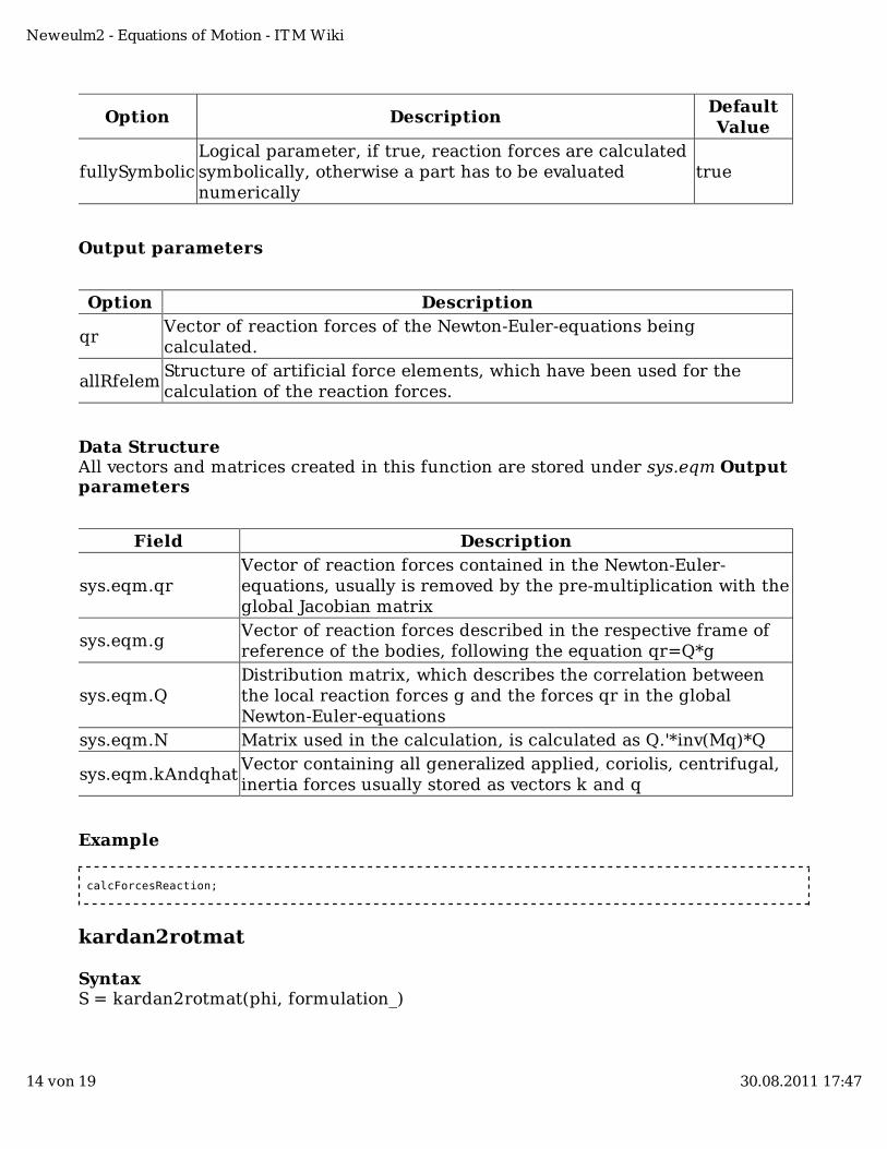
Option DescriptionDefaultValue
fullySymbolicLogical parameter, if true, reaction forces are calculatedsymbolically, otherwise a part has to be evaluatednumerically
true
Output parameters
Option Description
qrVector of reaction forces of the Newton-Euler-equations beingcalculated.
allRfelemStructure of artificial force elements, which have been used for thecalculation of the reaction forces.
Data StructureAll vectors and matrices created in this function are stored under sys.eqm Outputparameters
Field Description
sys.eqm.qrVector of reaction forces contained in the Newton-Euler-equations, usually is removed by the pre-multiplication with theglobal Jacobian matrix
sys.eqm.gVector of reaction forces described in the respective frame ofreference of the bodies, following the equation qr=Q*g
sys.eqm.QDistribution matrix, which describes the correlation betweenthe local reaction forces g and the forces qr in the globalNewton-Euler-equations
sys.eqm.N Matrix used in the calculation, is calculated as Q.'*inv(Mq)*Q
sys.eqm.kAndqhatVector containing all generalized applied, coriolis, centrifugal,inertia forces usually stored as vectors k and q
Example
calcForcesReaction;
kardan2rotmat
SyntaxS = kardan2rotmat(phi, formulation_)
Neweulm2 - Equations of Motion - ITM Wiki
14 von 19 30.08.2011 17:47
DescriptionWhen the user specifies a three parametric angular description, this function is usedto obtain the rotation matrix. As a standard, kardan angles (rotation order: x-y-z) areused. However, any description using three parameters can be used by specifyingthe order of the rotation axis, e.g. 'zxz', [1 2 3]. The function rotmat2kardan coversthe inverse operation.
Data StructureNo entry
Example
S = kardan2rotmat(sym('[a1;b1;c1]'), 'xyz');
rotmat2kardan
Syntaxphi = rotmat2kardan(S, useSimplify, formulation_)
DescriptionFrom a given rotation matrix, this function extracts the three parameter angulardescription. As a standard, kardan angles (rotation order: x-y-z) are used. However,any description using three parameters can be used by specifying the order of therotation axis, e.g. 'zxz', [1 2 3]. The function kardan2rotmat covers the inverseoperation.
Data StructureNo entry
Example
phi = rotmat2kardan(sym('[1,0,0;0,cos(a1),-sin(a1);0,sin(a1),cos(a1)]'), true, 'xyz')
relativeKinematics
SyntaxrelativeKinematics(y,Dy,D2y,Yvars_,Yvars_D_,ksys)
DescriptionCalculates the relative kinematic values of all coordinate systems recursively,y,Dy,D2y are symbolic vectors containing the generalized coordinates, their timederivatives respectively. yt is a taylor-series expansion up to the second order termsof the generalized coordinates. Yvars_, Yvars_D_ contain the state dependentparameters and their directional derivatives. ksys has to be passed as the startcoordinate system because of the recursive algorithm. Depending on the type of thecoordinate system the subfunctions calcKinRel, calcKinRelNode are called.
Neweulm2 - Equations of Motion - ITM Wiki
15 von 19 30.08.2011 17:47
Data StructureThe results are stored in the respective coordinate systems under sys.ksys.(...).relkin
absoluteKinematics
SyntaxabsoluteKinematics(ksys)
DescriptionStarting from the relative kinematic values calculated by relativeKinematics absolutekinemativ values and values necessary for the equations of motion are calculated.Some interesting kinematic values can be obtained via the functiongetAbsoluteKinematics at need. This has been introduced to calculate them onlywhen necessary and not always.
Data StructureThe results are stored in the respective coordinate systems. Depending on thecalculation mode and the frame type the respective reference system is different.Let's have a look at the coordinate system named ksys with the reference systemrefsys and ISYS shall denote the inertial system. For flexible bodies refsys denotesthe frame which describes the nonlinear reference motion. The first column givesthe name of the substructure in 'sys.ksys.ksys '. The second column denotes thefields of these substructures, whereas in the remaining columns the coordinatesystems in which the vector/matrix is described are given. If a field is left empty,this means that this value is not calculated by default.
Structureentry
Value
AbsoluteKinematics
'abs'
RelativeKinematics
'rel'
Nodalframe'rel'
symkin r_rel refsys refsys refsyssymkin phi_rel refsys refsys refsyssymkin/numkin r ISYS ISYS ISYSsymkin/numkin S ISYS ISYS ISYSsymkin/numkin S_rel refsys refsys refsyssymkin/numkin v ISYS ISYS ISYSsymkin/numkin a ISYS ISYS ISYSsymkin/numkin omega ISYS ISYS ISYSsymkin/numkin alpha ISYS ISYS ISYScalckin v ISYS ksys ksyscalckin a ISYS ksys ksyscalckin omega ISYS ksys ksyscalckin alpha ISYS ksys ksyscalcKin phi ISYS ksys ksys
Neweulm2 - Equations of Motion - ITM Wiki
16 von 19 30.08.2011 17:47
calckin vq ISYS ksys ksyscalckin aq ISYS ksys ksyscalckin omegaq ISYS ksys ksyscalckin alphaq ISYS ksys ksyscalckin Jt ISYS ksys ksyscalckin Jr ISYS ksys ksyscalckin Je ksyscalckin Jges ksyscalckin Tt ksyscalckin Tr ksys
If the relative kinematics are selected the equations of motion are set up in eachlocal coordinate system. For a rigid body this means in the frame in the center ofgravity. For a flexible body this means in the reference frame. The reason why thevalues just mentioned are in this case all described in ksys itself is to ensure aneasier code. If a body is defined from a nodal frame, this body will require the valuesof its reference frame, like velocity or jacobian matrix. If there were a differencebetween a rigid and a flexible body in the way in which the kinematical data isstored, this would require some distinction at this point.
getabsoluteKinematics
Syntax[result_,commonCSys] = getAbsoluteKinematics(kinematic, ksysFrom, ksysTo)
DescriptionIt is reasonable to calculate only those absolute kinematic values which are actuallynecessary. This function provides the possibility to calculate symbolic expressionswhich are not calculated as a standard. Please see the function itself for whichvalues are available, as this is still growing. The kinematic value should be specifiedas kinematic, and the two coordinate systems from and to which this value shall beevaluated symbolically. As the shortest available connection via the organizationaltree of the coordinate systems is used, they are discribed in the commonCSys, whichdenotes the first coordinate system, where the two branches meet. If ISYS is one ofthe given coordinate systems, it will always be commonCSys as well.
Data StructureIf one of the two coordinate systems is ISYS the resulting absolute values will bestored under sys.ksys.(...).symkin.
Example
[r, commonCSys] = getAbsoluteKinematics('r', 'ISYS', 'ksys1');
Neweulm2 - Equations of Motion - ITM Wiki
17 von 19 30.08.2011 17:47
mapleSimplify
Syntaxres = mapleSimplify(expr,varargin)
DescriptionWrapper function to call the simplify command. The existance of this file enables theseamless switching between using Maple or MuPad as symbolic engine.
Data StructureNo entry
Example
res = mapleSimplify(sym('x1^2+6*x1+9'))
mapleSubs
Syntaxres = mapleSubs(expr,old,new)
DescriptionWrapper function to call the subs or eval command to either replace symbolicparameters or to evaluate symbolic expressions. The existance of this file enables theseamless switching between using Maple or MuPad as symbolic engine.
Data StructureNo entry
Example
res = mapleSubs(sym('x1^2+6*x1+9'),sym('x1'),sym('y2'))
writeStructure
SyntaxwriteStructure(structure)
DescriptionHandy function to simply write a structure. If nothing is specified, STDOUT is usedfor the fprintf commands. Can also be written to a file. The result is a printout of allsubstructures and fields together with its values so it could be evaluated to obtainthe original data structure.
Data StructureNo entry
Neweulm2 - Equations of Motion - ITM Wiki
18 von 19 30.08.2011 17:47
Example
writeStructure(sys.par.eqm)
See also
ITM Wiki
neweulm2neweulm2#Function reference
neweulm2 - System Definitionneweulm2 - Simulation and Animationneweulm2 - Exporting
Retrieved from "http://www.itm.uni-stuttgart.de/itmwiki/index.php/Neweulm2_-_Equations_of_Motion"
This page was last modified 15:09, 30 August 2011.
Neweulm2 - Equations of Motion - ITM Wiki
19 von 19 30.08.2011 17:47
Neweulm2 - Simulation andAnimation
From ITM Wiki
Neweul-M² can be used just to create equations of motion and the correspondingm-files. But it also offers a great variety of possibilities for simulation andanimation which will be presented in this paragraph.
Contents
1 Simulation and Analysis1.1 freqResPlot1.2 fullModelRun1.3 newOpt1.4 optiEvalFreqRes1.5 plotStandardResults1.6 printSystemInformation1.7 runKiAn1.8 runModalAnalysis1.9 runTimeInt1.10 runSensAn1.11 runSysOpt
2 Auxiliary functions for the simulation2.1 calcNomLength2.2 freqResponse2.3 initOpt2.4 kinematicAnalysis2.5 modalAnalysis2.6 staticEquilibrium2.7 timeInt2.8 writeFinalCond
3 Animation3.1 Functions to be called directly by the user
3.1.1 addGraphics3.1.2 animFreqResponse3.1.3 animModeShape3.1.4 animTimeInt
Neweulm2 - Simulation and Animation - ITM Wiki http://www.itm.uni-stuttgart.de/itmwiki/index.php?ti...
1 von 26 11.11.2011 18:06
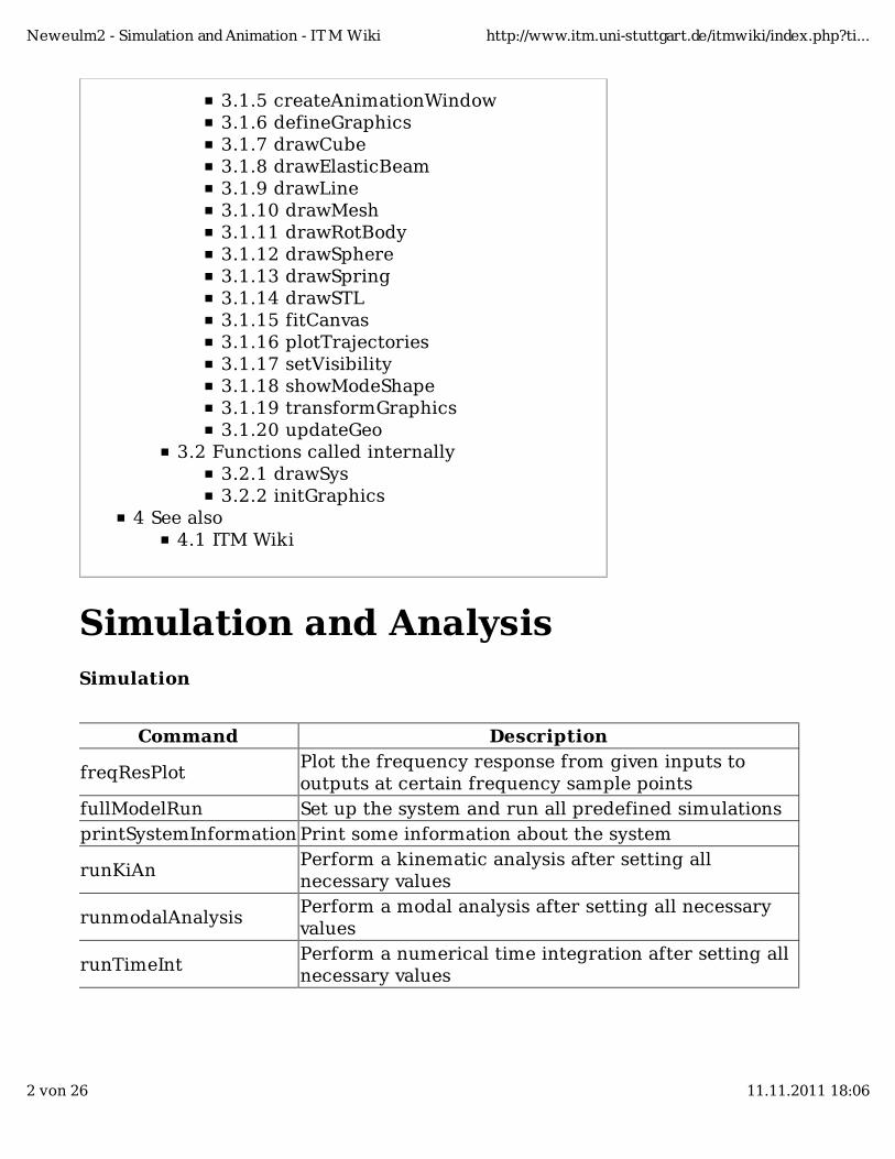
3.1.5 createAnimationWindow3.1.6 defineGraphics3.1.7 drawCube3.1.8 drawElasticBeam3.1.9 drawLine3.1.10 drawMesh3.1.11 drawRotBody3.1.12 drawSphere3.1.13 drawSpring3.1.14 drawSTL3.1.15 fitCanvas3.1.16 plotTrajectories3.1.17 setVisibility3.1.18 showModeShape3.1.19 transformGraphics3.1.20 updateGeo
3.2 Functions called internally3.2.1 drawSys3.2.2 initGraphics
4 See also4.1 ITM Wiki
Simulation and AnalysisSimulation
Command Description
freqResPlotPlot the frequency response from given inputs tooutputs at certain frequency sample points
fullModelRun Set up the system and run all predefined simulationsprintSystemInformation Print some information about the system
runKiAnPerform a kinematic analysis after setting allnecessary values
runmodalAnalysisPerform a modal analysis after setting all necessaryvalues
runTimeIntPerform a numerical time integration after setting allnecessary values
Neweulm2 - Simulation and Animation - ITM Wiki http://www.itm.uni-stuttgart.de/itmwiki/index.php?ti...
2 von 26 11.11.2011 18:06
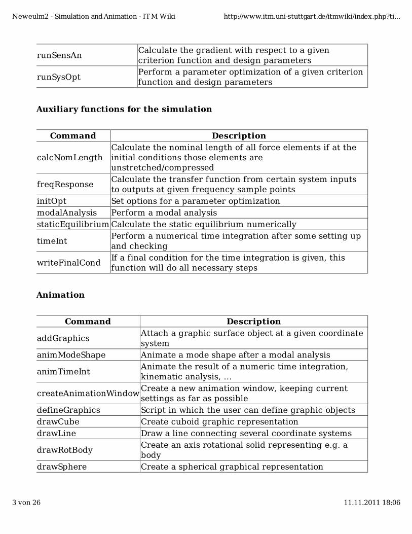
runSensAnCalculate the gradient with respect to a givencriterion function and design parameters
runSysOptPerform a parameter optimization of a given criterionfunction and design parameters
Auxiliary functions for the simulation
Command Description
calcNomLengthCalculate the nominal length of all force elements if at theinitial conditions those elements areunstretched/compressed
freqResponseCalculate the transfer function from certain system inputsto outputs at given frequency sample points
initOpt Set options for a parameter optimizationmodalAnalysis Perform a modal analysisstaticEquilibrium Calculate the static equilibrium numerically
timeIntPerform a numerical time integration after some setting upand checking
writeFinalCondIf a final condition for the time integration is given, thisfunction will do all necessary steps
Animation
Command Description
addGraphicsAttach a graphic surface object at a given coordinatesystem
animModeShape Animate a mode shape after a modal analysis
animTimeIntAnimate the result of a numeric time integration,kinematic analysis, ...
createAnimationWindowCreate a new animation window, keeping currentsettings as far as possible
defineGraphics Script in which the user can define graphic objectsdrawCube Create cuboid graphic representationdrawLine Draw a line connecting several coordinate systems
drawRotBodyCreate an axis rotational solid representing e.g. abody
drawSphere Create a spherical graphical representation
Neweulm2 - Simulation and Animation - ITM Wiki http://www.itm.uni-stuttgart.de/itmwiki/index.php?ti...
3 von 26 11.11.2011 18:06
drawSTLRead data from a CAD geometry file (.stl) and createa graphical representation from it
fitCanvasAdjust the axis scaling so the animation will stayvisible during its run
plot_trajectoriesFunction to create and update trajectories ofcoordinate systems
setVisibilityChange visibility settings of all objects or classes ofobjects in the animation window
showModeShape Statically display mode shapes of a modal analysis
transformGraphicsBefore attaching graphic representations to acoordinate system, this function can give them aconstant translational or rotational offset
updateGeoUpdate the animation window to a certain time andset of generalized coordinates
Auxiliary functions for the animation
Command Description
drawSysCreate all necessary representations for a system in theanimation window, called from createAnimationWindow
initGraphicsInitialize settings and create an animation window, called fromcreateAnimationWindow
freqResPlot
Syntax[fh,ah,g] = freqResPlot(t,in,out,freqs,varargin);
DescriptionCreates a bode plot of the frequency response at given time t, from input in tooutput out for frequencies freqs. In varargin other options can be passed. Itreturns the figure fh, axes handles ah and the frequency response matrix g.Uses the function frequencyResponse to evaluate the transfer functions.Optional input arguments provide access to several settings like using certaingroups of in- or outputs.
Data StructureNo entry
Neweulm2 - Simulation and Animation - ITM Wiki http://www.itm.uni-stuttgart.de/itmwiki/index.php?ti...
4 von 26 11.11.2011 18:06
Example
freqRespPlot;freqRespPlot(0,'MyInput','MyOutput',[1:10:100]);
fullModelRun
SyntaxfullModelRun(varargin);
DescriptionWhen a user does not yet know exactly how to use the software, this command isvery useful. When it is called from an examples folder, first the system definitionis called and the equations are set up. Then all available simulations for thismodel are called. This allows the user to easily call the provided files and toinvestigate the system later. This function is also called by the graphicalgettingStarted user interface.
Data StructureNo entry
Example
fullModelRun;fullModelRun('DisplayCommands',true);
newOpt
Syntax[res_, opts] = newOpt(varargin);
DescriptionThis function combines all currently available ways for a parameter optimizationor sensitivity analysis in one function. This incorporates the previously usedfunctions optiEvalFreqRes, runSensAn and runSysOpt. Here all options storedunder sys.par.opt are used, but the user can specify options in the usualpairwise manner.
Data Structuresys.results.opt
Example
newOpt;
Neweulm2 - Simulation and Animation - ITM Wiki http://www.itm.uni-stuttgart.de/itmwiki/index.php?ti...
5 von 26 11.11.2011 18:06
optiEvalFreqRes
Syntaxres_ = optiEvalFreqRes(varargin);
DescriptionThere are many ways to conduct a parameter optimization of a mechanicalsystem. One very fast and useful way is to use the transfer functions betweensystem in- and outputs. Of course this uses a linear system formulation, which isnot always suitable. But the great advantage is the speed and the simple usageof many transfer functions at once. As a standard, all available transferfunctions are evaluated at the given frequencies, then for each frequency themaximum amplitude of all functions is determined. Over the complete set offrequency points, a certain number of maximum values is selected. These pointsrepresent the most critical combinations of transfer function and frequency. Thedouble selection is necessary to avoid a certain independency from the numberof system in- and outputs and frequency set points. For the selected points, theamplitudes of the transfer functions is summed and used as a criterion. Thisselection process is conducted in every optimization step, which has shown to bequite a good way to cover even complex systems. The design parameters arescaled to ensure good behavior of the optimization algorithm. All options are setin initOpt.m or any other options file, then being specified explicitly.
Data Structuresys.results.opt
Example
optiEvalFreqRes;
plotStandardResults
SyntaxplotStandardResults('Option1','Value1');
DescriptionIf you want to plot any curve derived from a result in Neweul-M², thisfunction is the place to try first.
Very often similar calculations and plots are carried out with Neweul-M². Thisfunction provides a selection of the plots which are created most often. Thisincludes plots of the states, trajectories of coordinate systems, system outputsand others. A complete list can be found in its help commentary. This function
Neweulm2 - Simulation and Animation - ITM Wiki http://www.itm.uni-stuttgart.de/itmwiki/index.php?ti...
6 von 26 11.11.2011 18:06
provides a large number of options, concerning both, the data to plot and itsformatting and output. A very useful feature is that the calculated data isavailable as second output argument. This provides a very simple way to obtaintrajectories, system outputs and other data at specific time points.
Data Structureno entry
Example
plotStandardResults;plotStandardResults('Type','constraints','subplot',true);
printSystemInformation
SyntaxprintSystemInformation('Option1','Value1');
DescriptionEven though Neweul-M² can handle very different types of systems, there aresome things which are good to know about systems. So this function wasdeveloped as a collection of commands to display information which I used tolook up for systems I could lay my hands on. For example when one of the usershad a problem with a model, then I used to look for some structure of thecoordinate systems, the generalized coordinates have been used in whichdefinitions, where do we have force elements, ... . At some point we created afunction which would display all this information with just one command. At alater point in time, this function was extended to also provide numericalinformation about the system, meaning positions, orientations, mass properties,... for given states. This is especially useful when a system has been modeled in adifferent software before or measured from a real structure. Then one can easilyverify the model by comparing the positions of some coordinate systems. Pleasetype help printSystemInformation for more information on how to adjust thefunction to your needs. This function can be called from the GUI from theSystem Information menu item.
Data Structureno entry
Example
printSystemInformation;printSystemInformation('all');printSystemInformation('numerical',true,'y0',0.1*ones(sys.dof,1));
Neweulm2 - Simulation and Animation - ITM Wiki http://www.itm.uni-stuttgart.de/itmwiki/index.php?ti...
7 von 26 11.11.2011 18:06
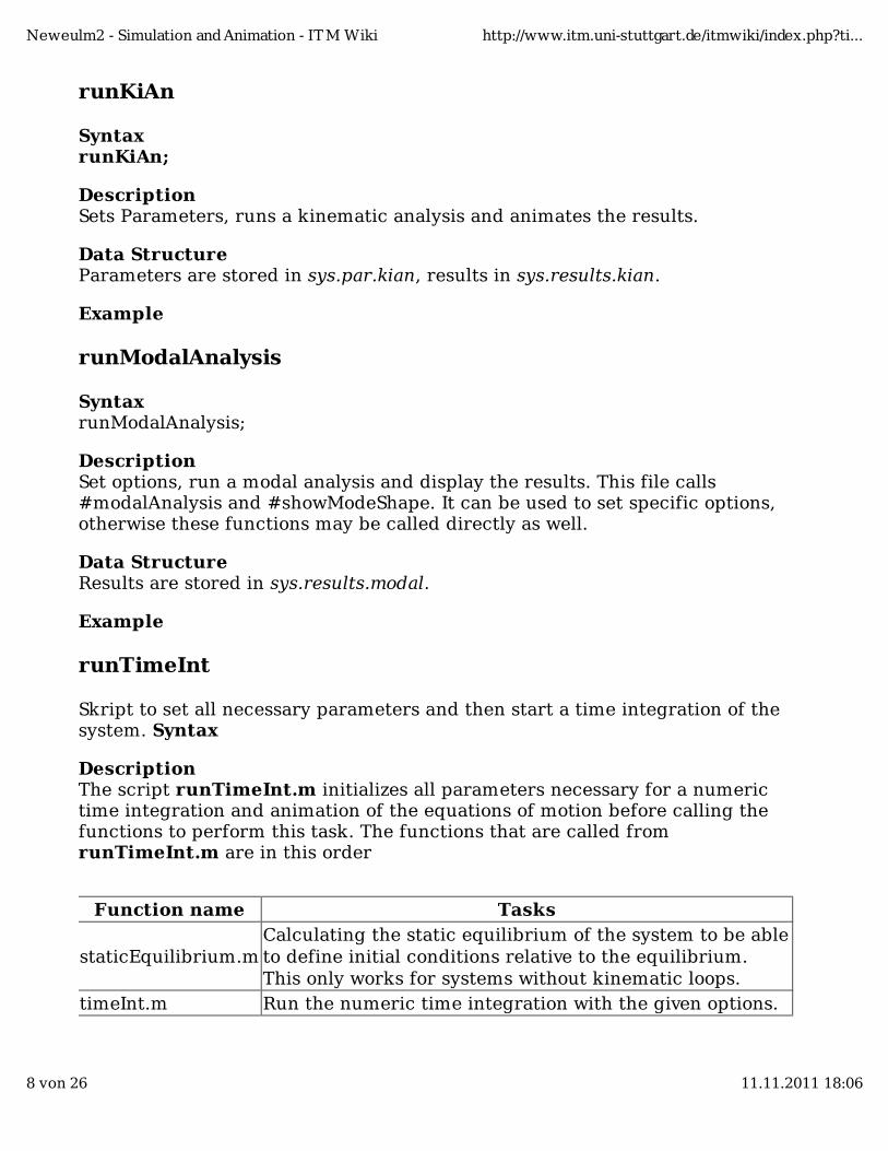
runKiAn
SyntaxrunKiAn;
DescriptionSets Parameters, runs a kinematic analysis and animates the results.
Data StructureParameters are stored in sys.par.kian, results in sys.results.kian.
Example
runModalAnalysis
SyntaxrunModalAnalysis;
DescriptionSet options, run a modal analysis and display the results. This file calls#modalAnalysis and #showModeShape. It can be used to set specific options,otherwise these functions may be called directly as well.
Data StructureResults are stored in sys.results.modal.
Example
runTimeInt
Skript to set all necessary parameters and then start a time integration of thesystem. Syntax
DescriptionThe script runTimeInt.m initializes all parameters necessary for a numerictime integration and animation of the equations of motion before calling thefunctions to perform this task. The functions that are called fromrunTimeInt.m are in this order
Function name Tasks
staticEquilibrium.mCalculating the static equilibrium of the system to be ableto define initial conditions relative to the equilibrium.This only works for systems without kinematic loops.
timeInt.m Run the numeric time integration with the given options.
Neweulm2 - Simulation and Animation - ITM Wiki http://www.itm.uni-stuttgart.de/itmwiki/index.php?ti...
8 von 26 11.11.2011 18:06
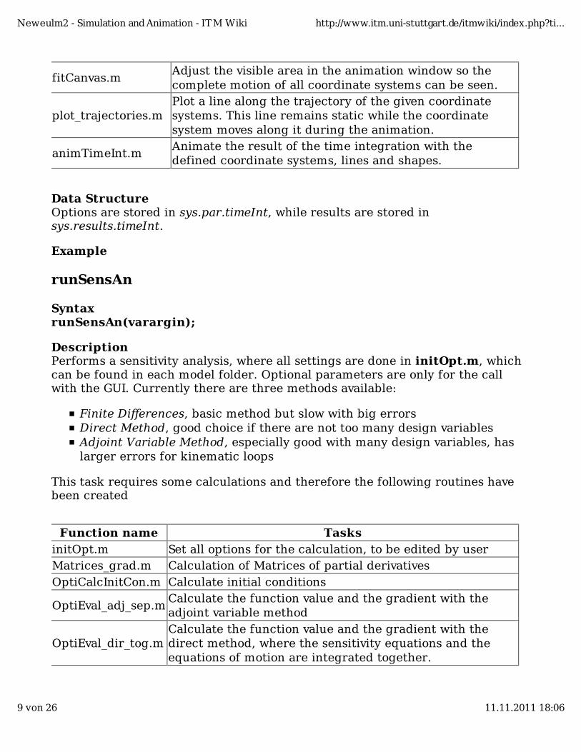
fitCanvas.mAdjust the visible area in the animation window so thecomplete motion of all coordinate systems can be seen.
plot_trajectories.mPlot a line along the trajectory of the given coordinatesystems. This line remains static while the coordinatesystem moves along it during the animation.
animTimeInt.mAnimate the result of the time integration with thedefined coordinate systems, lines and shapes.
Data StructureOptions are stored in sys.par.timeInt, while results are stored insys.results.timeInt.
Example
runSensAn
SyntaxrunSensAn(varargin);
DescriptionPerforms a sensitivity analysis, where all settings are done in initOpt.m, whichcan be found in each model folder. Optional parameters are only for the callwith the GUI. Currently there are three methods available:
Finite Differences, basic method but slow with big errorsDirect Method, good choice if there are not too many design variablesAdjoint Variable Method, especially good with many design variables, haslarger errors for kinematic loops
This task requires some calculations and therefore the following routines havebeen created
Function name TasksinitOpt.m Set all options for the calculation, to be edited by userMatrices_grad.m Calculation of Matrices of partial derivativesOptiCalcInitCon.m Calculate initial conditions
OptiEval_adj_sep.mCalculate the function value and the gradient with theadjoint variable method
OptiEval_dir_tog.mCalculate the function value and the gradient with thedirect method, where the sensitivity equations and theequations of motion are integrated together.
Neweulm2 - Simulation and Animation - ITM Wiki http://www.itm.uni-stuttgart.de/itmwiki/index.php?ti...
9 von 26 11.11.2011 18:06
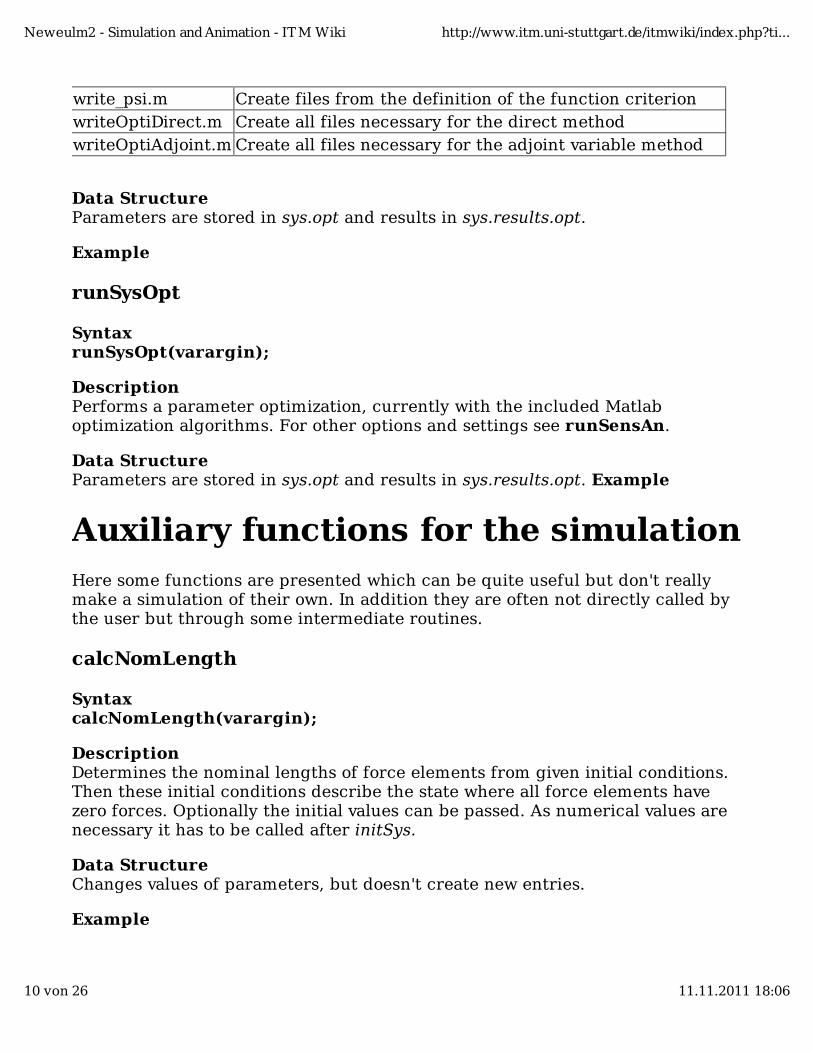
write_psi.m Create files from the definition of the function criterionwriteOptiDirect.m Create all files necessary for the direct methodwriteOptiAdjoint.m Create all files necessary for the adjoint variable method
Data StructureParameters are stored in sys.opt and results in sys.results.opt.
Example
runSysOpt
SyntaxrunSysOpt(varargin);
DescriptionPerforms a parameter optimization, currently with the included Matlaboptimization algorithms. For other options and settings see runSensAn.
Data StructureParameters are stored in sys.opt and results in sys.results.opt. Example
Auxiliary functions for the simulationHere some functions are presented which can be quite useful but don't reallymake a simulation of their own. In addition they are often not directly called bythe user but through some intermediate routines.
calcNomLength
SyntaxcalcNomLength(varargin);
DescriptionDetermines the nominal lengths of force elements from given initial conditions.Then these initial conditions describe the state where all force elements havezero forces. Optionally the initial values can be passed. As numerical values arenecessary it has to be called after initSys.
Data StructureChanges values of parameters, but doesn't create new entries.
Example
Neweulm2 - Simulation and Animation - ITM Wiki http://www.itm.uni-stuttgart.de/itmwiki/index.php?ti...
10 von 26 11.11.2011 18:06
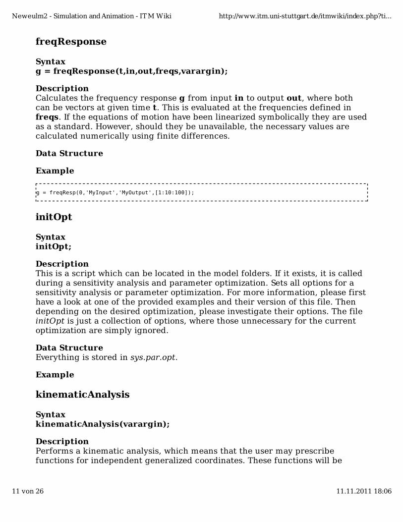
freqResponse
Syntaxg = freqResponse(t,in,out,freqs,varargin);
DescriptionCalculates the frequency response g from input in to output out, where bothcan be vectors at given time t. This is evaluated at the frequencies defined infreqs. If the equations of motion have been linearized symbolically they are usedas a standard. However, should they be unavailable, the necessary values arecalculated numerically using finite differences.
Data Structure
Example
g = freqResp(0,'MyInput','MyOutput',[1:10:100]);
initOpt
SyntaxinitOpt;
DescriptionThis is a script which can be located in the model folders. If it exists, it is calledduring a sensitivity analysis and parameter optimization. Sets all options for asensitivity analysis or parameter optimization. For more information, please firsthave a look at one of the provided examples and their version of this file. Thendepending on the desired optimization, please investigate their options. The fileinitOpt is just a collection of options, where those unnecessary for the currentoptimization are simply ignored.
Data StructureEverything is stored in sys.par.opt.
Example
kinematicAnalysis
SyntaxkinematicAnalysis(varargin);
DescriptionPerforms a kinematic analysis, which means that the user may prescribefunctions for independent generalized coordinates. These functions will be
Neweulm2 - Simulation and Animation - ITM Wiki http://www.itm.uni-stuttgart.de/itmwiki/index.php?ti...
11 von 26 11.11.2011 18:06
evaluated, which can be used to investigate special configurations, reachablespace of a robot or other such things. Please note, that here only the kinematicsis investigated, meaning that all forces, torques or other effects are neglected.Constraint equations are respected.
Data Structuresys.results.kian
Example
kinematicAnalysis;
modalAnalysis
SyntaxmodalAnalysis(t,varargin);
DescriptionPerforms a modal analysis of the system with the default settings and withoutdisplay. For a display of the Eigenmodes please see showModeShape. TheParameter t defines the time at which the matrices are evaluated. No optionalparameters available yet.
Data Structuresys.results.modal
Example
modalAnalysis(0);
staticEquilibrium
Syntax[ye,res] = staticEquilibrium(t,ys,Options);
DescriptionCalculates the static equilibrium ye of the system at time t to initial guess ys.The residual of this root finding is returned as res, which should be zeros. InOptions additional options for the root finding can be passed. All parametersare optional.
Data StructureResults are to be stored in sys.results.statEq, has to be selected by the user.
Example
Neweulm2 - Simulation and Animation - ITM Wiki http://www.itm.uni-stuttgart.de/itmwiki/index.php?ti...
12 von 26 11.11.2011 18:06
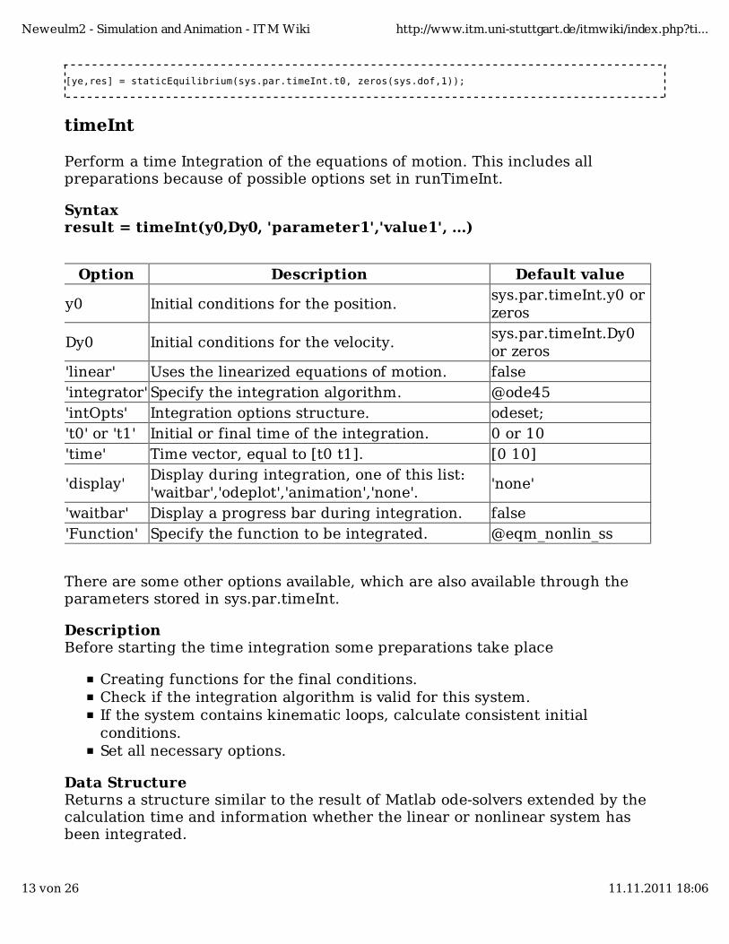
[ye,res] = staticEquilibrium(sys.par.timeInt.t0, zeros(sys.dof,1));
timeInt
Perform a time Integration of the equations of motion. This includes allpreparations because of possible options set in runTimeInt.
Syntaxresult = timeInt(y0,Dy0, 'parameter1','value1', ...)
Option Description Default value
y0 Initial conditions for the position.sys.par.timeInt.y0 orzeros
Dy0 Initial conditions for the velocity.sys.par.timeInt.Dy0or zeros
'linear' Uses the linearized equations of motion. false'integrator' Specify the integration algorithm. @ode45'intOpts' Integration options structure. odeset;'t0' or 't1' Initial or final time of the integration. 0 or 10'time' Time vector, equal to [t0 t1]. [0 10]
'display'Display during integration, one of this list:'waitbar','odeplot','animation','none'.
'none'
'waitbar' Display a progress bar during integration. false'Function' Specify the function to be integrated. @eqm_nonlin_ss
There are some other options available, which are also available through theparameters stored in sys.par.timeInt.
DescriptionBefore starting the time integration some preparations take place
Creating functions for the final conditions.Check if the integration algorithm is valid for this system.If the system contains kinematic loops, calculate consistent initialconditions.Set all necessary options.
Data StructureReturns a structure similar to the result of Matlab ode-solvers extended by thecalculation time and information whether the linear or nonlinear system hasbeen integrated.
Neweulm2 - Simulation and Animation - ITM Wiki http://www.itm.uni-stuttgart.de/itmwiki/index.php?ti...
13 von 26 11.11.2011 18:06
Example
sys.results.timeInt = timeInt(y0, Dy0);sys.results.timeInt = timeInt(ones(sys.dof,1),zeros(sys.dof,1), 'integrator',@ode45, ... 'intOpts',odeset, 'time',[0,10], 'linear',' ');
writeFinalCond
SyntaxwriteFinalCond
DescriptionUsually the time integration goes over the complete time interval [t0, t1]. Thisfunction enables the user to define a condition, so the integration can bestopped when a certain condition changes its sign. If a final condition for thetime integration is stored in the structure sys, this creates the necessary file(sysFunctions/finalCond.m) and options.
Data StructureThe final condition is stored in sys.par.timeInt.finalCond
Example
Animation
Functions to be called directly by the user
addGraphics
SyntaxaddGraphics(CoordSys, ObjectHandle, createEntry);
DescriptionAttaches created primitives with handle ObjectHandle to a given coordinatesystem CoordSys. With the boolean parameter createEntry the insertion intothe system data structure can be avoided. Otherwise all surface or patch objectsare stored in sys.graphics.surfaces
Data Structuresys.graphics.surfaces
Example
Neweulm2 - Simulation and Animation - ITM Wiki http://www.itm.uni-stuttgart.de/itmwiki/index.php?ti...
14 von 26 11.11.2011 18:06
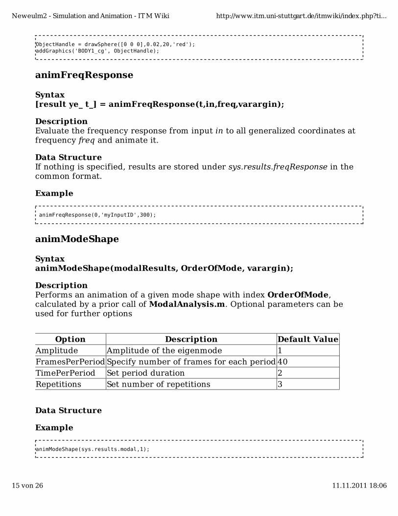
ObjectHandle = drawSphere([0 0 0],0.02,20,'red');addGraphics('BODY1_cg', ObjectHandle);
animFreqResponse
Syntax[result ye_ t_] = animFreqResponse(t,in,freq,varargin);
DescriptionEvaluate the frequency response from input in to all generalized coordinates atfrequency freq and animate it.
Data StructureIf nothing is specified, results are stored under sys.results.freqResponse in thecommon format.
Example
animFreqResponse(0,'myInputID',300);
animModeShape
SyntaxanimModeShape(modalResults, OrderOfMode, varargin);
DescriptionPerforms an animation of a given mode shape with index OrderOfMode,calculated by a prior call of ModalAnalysis.m. Optional parameters can beused for further options
Option Description Default ValueAmplitude Amplitude of the eigenmode 1FramesPerPeriod Specify number of frames for each period 40TimePerPeriod Set period duration 2Repetitions Set number of repetitions 3
Data Structure
Example
animModeShape(sys.results.modal,1);
Neweulm2 - Simulation and Animation - ITM Wiki http://www.itm.uni-stuttgart.de/itmwiki/index.php?ti...
15 von 26 11.11.2011 18:06
animTimeInt
Animation of results of a time integration or similarly stored results.
SyntaxanimTimeInt(tisol, 'Parameter1','Value1', 'Parameter2','Value2')
DescriptionAnimates the motion described by a result as from a time integration. Thereforealso the result of a kinematic analysis can be used.
Parameter DescriptionDefaultvalue
tisol Structure with integration result as of ode45 -'TimeStep' Stepsize for animation time 'Optimal''Stride' Real time factor, e.g. slow motion 1
'CenterCS'Centers the view during the animation to thisCoordinate system
-
'Record_avi'Records animation, i.e. a movie, to the.avi-filename passed as argument
-
'Print_frames'Print all frames of the animation to the folderspecified as second value
-
'Resolution' Set resolution for 'Print_frames' in dpi 600
'plot_trajectories'Usually the trajectories are updatedautomatically, but can be switched off
true
If 'TimeStep' is passed with 'Optimal' as an argument the optimal time step sizeis decided automatically. If nothing is specified, the result of the timeintegration is used.
Data Structure
Example
animTimeInt;
createAnimationWindow
SyntaxcreateAnimationWindow(varargin);
Description
Neweulm2 - Simulation and Animation - ITM Wiki http://www.itm.uni-stuttgart.de/itmwiki/index.php?ti...
16 von 26 11.11.2011 18:06
If an animation window exists, it is closed. All other plot windows are unaffected.Then a new animation window is made, including any previously defined graphicobjects, no matter if lines, markers, surfaces, patches, ... . This function wascreated to simplify the creation of an animation window. Therefore no matterwhat is available, exists or has been defined previously, this function is meant torecreate it as close as possible. Therefore all settings should be checked so italways works. Currently no options are available.
Data Structure
Example
createAnimationWindow;
defineGraphics
SyntaxdefineGraphics
DescriptionScript which the user has to write, to define graphic visualizations of the bodies.This includes the creation of primitives described below, e.g.
drawCube Draw cuboidsdrawLine Draw lines connecting two coordinate systemsdrawRotBody Draw rotational bodies, open or closeddrawSphere Draw spheresdrawSTL Read .stl files from CAD-softwares and draw corresponding shapestransformGraphics Transform graphic objects in position and orientationwith respect to their governing coordinate system. This function is forconstant offsets not for an animation.
Data Structure
Example
drawCube
Syntaxh = drawCube(CenterVect,dx,dy,dz,color,varargin);
DescriptionCreates a cuboid in the animation window with handle h. This cuboid is centeredat CenterVect(1x3), with the side lengths dx, dy, dz and a given color. It has tobe attached to a coordinate system with addGraphics.
Neweulm2 - Simulation and Animation - ITM Wiki http://www.itm.uni-stuttgart.de/itmwiki/index.php?ti...
17 von 26 11.11.2011 18:06
As optional input arguments the following are possible
Option DescriptionDefaultValue
Tag Specify the tag of this object 'Cube'
FaceColorColor of the faces, overwrites the previously givencolor, available to unify creation of shapes.
[0 0 1]
EdgeColor Color of the edges 'none'Color Set face and edge color -FaceAlpha Set transparency of the faces 1EdgeAlpha Set transparency of the edges 1
Data StructureNo entry
Example
h = drawCube([0 0 0], 0.3,0.1,0.1, 'blue');
drawElasticBeam
Syntaxhandle = drawElasticBeam(lineID, varargin);
DescriptionAfter adding a line element with drawLine this function can be used to asign acertain crosssection to this line. The crosssection can be specified arbitrarily orone of the predefined ones (rectangle, circle or triangle can be used. If desiredthe faces can be removed by setting the 'FaceColor' option to 'none' or they canbe transparent. As is common, non-required options are to be given inargument/value pairs.
Data StructureSee sys.graphics.surfaces.
Example
drawElasticBeam('myLine','Sidelengths',0.1);drawElasticBeam('myLine','Triangle',0.15,'FaceColor','none');
drawLine
Neweulm2 - Simulation and Animation - ITM Wiki http://www.itm.uni-stuttgart.de/itmwiki/index.php?ti...
18 von 26 11.11.2011 18:06
Syntax[handle, error_msg] = drawLine(ListofFrames, ID, varargin);
DescriptionAdds a line object to the animation window, which connects the coordinatesystems specified in ListofFrames. If two are given, they are connected with astraight line, more coordinate systems are connected by splines. Foridentification it is assigned an ID, other options are optional in varargin. Theseadditional options are to be given pairwise and all of Matlab's line options areavailable, as they are passed straight through.
Data StructureSee sys.graphics.line.
Example
drawLine({'BODY1', 'BODY2_cg'}, 'MyLine','Color',[0 1 1]);
drawMesh
Syntaxh = drawMesh(ID_,varargin)
DescriptionDepending on the software used to model the elastic bodies and perform themodel reduction, so called 'mesh' data is available. This is usually the completeouter surface of the elastic body, which can then be used for an animation. Ifsuch data is available, this function is called automatically at body definition.This function also provides options to change settings like the color of thegraphical representation.
Data StructureSee sys.graphics.surfaces.Mesh_1.
Example
drawMesh('BODY1','FaceColor',[1 0 0])
drawRotBody
Syntaxh = drawRotBody(rvec,zvec,varargin)
DescriptionCreates a rotational solid in the animation window with handle h. The
Neweulm2 - Simulation and Animation - ITM Wiki http://www.itm.uni-stuttgart.de/itmwiki/index.php?ti...
19 von 26 11.11.2011 18:06
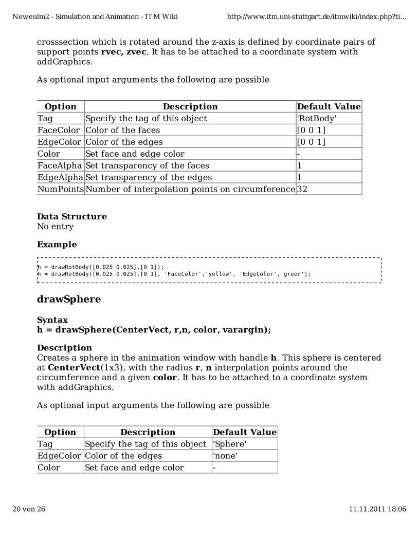
crosssection which is rotated around the z-axis is defined by coordinate pairs ofsupport points rvec, zvec. It has to be attached to a coordinate system withaddGraphics.
As optional input arguments the following are possible
Option Description Default ValueTag Specify the tag of this object 'RotBody'FaceColor Color of the faces [0 0 1]EdgeColor Color of the edges [0 0 1]Color Set face and edge color -FaceAlpha Set transparency of the faces 1EdgeAlpha Set transparency of the edges 1NumPoints Number of interpolation points on circumference 32
Data StructureNo entry
Example
h = drawRotBody([0.025 0.025],[0 1]);h = drawRotBody([0.025 0.025],[0 1], 'FaceColor','yellow', 'EdgeColor','green');
drawSphere
Syntaxh = drawSphere(CenterVect, r,n, color, varargin);
DescriptionCreates a sphere in the animation window with handle h. This sphere is centeredat CenterVect(1x3), with the radius r, n interpolation points around thecircumference and a given color. It has to be attached to a coordinate systemwith addGraphics.
As optional input arguments the following are possible
Option Description Default ValueTag Specify the tag of this object 'Sphere'EdgeColor Color of the edges 'none'Color Set face and edge color -
Neweulm2 - Simulation and Animation - ITM Wiki http://www.itm.uni-stuttgart.de/itmwiki/index.php?ti...
20 von 26 11.11.2011 18:06
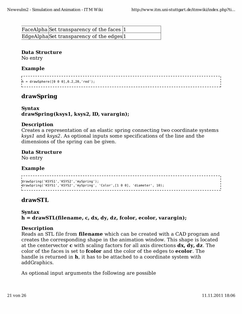
FaceAlpha Set transparency of the faces 1EdgeAlpha Set transparency of the edges 1
Data StructureNo entry
Example
h = drawSphere([0 0 0],0.2,20,'red');
drawSpring
SyntaxdrawSpring(ksys1, ksys2, ID, varargin);
DescriptionCreates a representation of an elastic spring connecting two coordinate systemsksys1 and ksys2. As optional inputs some specifications of the line and thedimensions of the spring can be given.
Data StructureNo entry
Example
drawSpring('KSYS1','KSYS2','mySpring');drawSpring('KSYS1','KSYS2','mySpring', 'Color',[1 0 0], 'diameter', 10);
drawSTL
Syntaxh = drawSTL(filename, c, dx, dy, dz, fcolor, ecolor, varargin);
DescriptionReads an STL file from filename which can be created with a CAD program andcreates the corresponding shape in the animation window. This shape is locatedat the centervector c with scaling factors for all axis directions dx, dy, dz. Thecolor of the faces is set to fcolor and the color of the edges to ecolor. Thehandle is returned in h, it has to be attached to a coordinate system withaddGraphics.
As optional input arguments the following are possible
Neweulm2 - Simulation and Animation - ITM Wiki http://www.itm.uni-stuttgart.de/itmwiki/index.php?ti...
21 von 26 11.11.2011 18:06
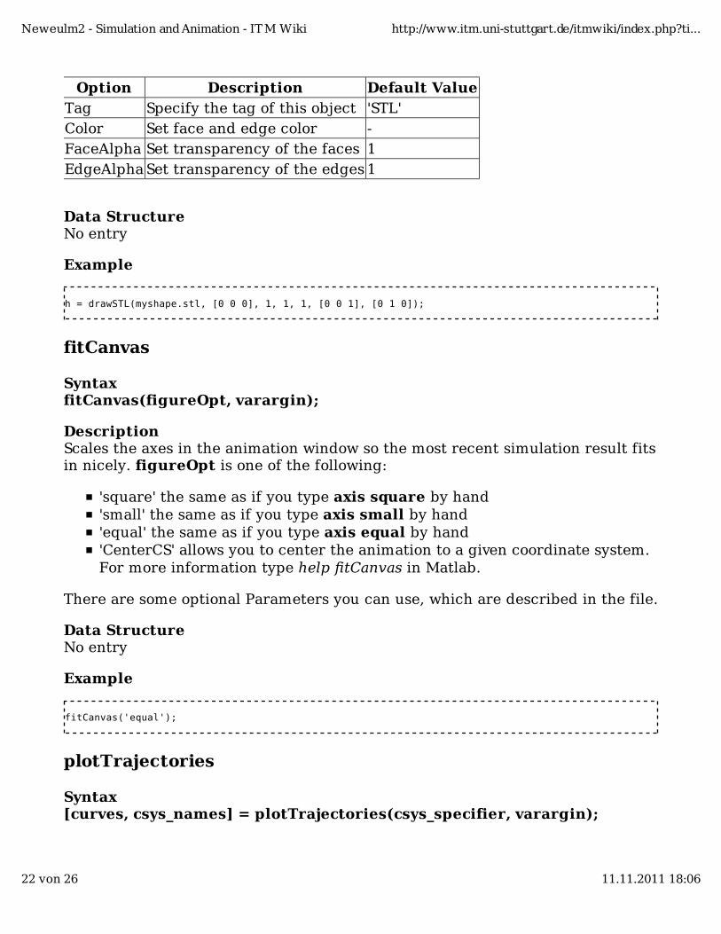
Option Description Default ValueTag Specify the tag of this object 'STL'Color Set face and edge color -FaceAlpha Set transparency of the faces 1EdgeAlpha Set transparency of the edges 1
Data StructureNo entry
Example
h = drawSTL(myshape.stl, [0 0 0], 1, 1, 1, [0 0 1], [0 1 0]);
fitCanvas
SyntaxfitCanvas(figureOpt, varargin);
DescriptionScales the axes in the animation window so the most recent simulation result fitsin nicely. figureOpt is one of the following:
'square' the same as if you type axis square by hand'small' the same as if you type axis small by hand'equal' the same as if you type axis equal by hand'CenterCS' allows you to center the animation to a given coordinate system.For more information type help fitCanvas in Matlab.
There are some optional Parameters you can use, which are described in the file.
Data StructureNo entry
Example
fitCanvas('equal');
plotTrajectories
Syntax[curves, csys_names] = plotTrajectories(csys_specifier, varargin);
Neweulm2 - Simulation and Animation - ITM Wiki http://www.itm.uni-stuttgart.de/itmwiki/index.php?ti...
22 von 26 11.11.2011 18:06
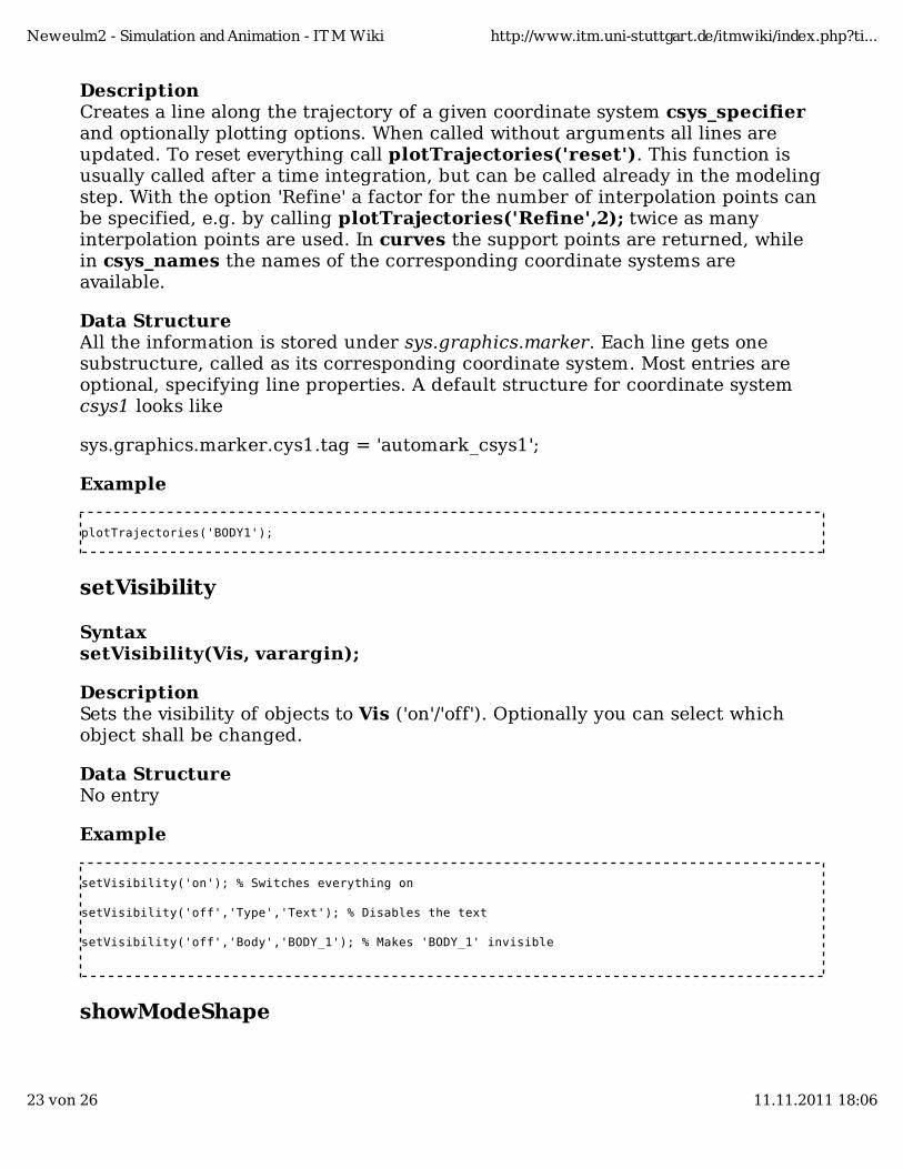
DescriptionCreates a line along the trajectory of a given coordinate system csys_specifierand optionally plotting options. When called without arguments all lines areupdated. To reset everything call plotTrajectories('reset'). This function isusually called after a time integration, but can be called already in the modelingstep. With the option 'Refine' a factor for the number of interpolation points canbe specified, e.g. by calling plotTrajectories('Refine',2); twice as manyinterpolation points are used. In curves the support points are returned, whilein csys_names the names of the corresponding coordinate systems areavailable.
Data StructureAll the information is stored under sys.graphics.marker. Each line gets onesubstructure, called as its corresponding coordinate system. Most entries areoptional, specifying line properties. A default structure for coordinate systemcsys1 looks like
sys.graphics.marker.cys1.tag = 'automark_csys1';
Example
plotTrajectories('BODY1');
setVisibility
SyntaxsetVisibility(Vis, varargin);
DescriptionSets the visibility of objects to Vis ('on'/'off'). Optionally you can select whichobject shall be changed.
Data StructureNo entry
Example
setVisibility('on'); % Switches everything on
setVisibility('off','Type','Text'); % Disables the text
setVisibility('off','Body','BODY_1'); % Makes 'BODY_1' invisible
showModeShape
Neweulm2 - Simulation and Animation - ITM Wiki http://www.itm.uni-stuttgart.de/itmwiki/index.php?ti...
23 von 26 11.11.2011 18:06
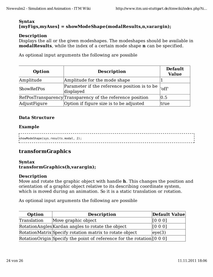
Syntax[myFigs,myAxes] = showModeShape(modalResults,n,varargin);
DescriptionDisplays the all or the given modeshapes. The modeshapes should be available inmodalResults, while the index of a certain mode shape n can be specified.
As optional input arguments the following are possible
Option DescriptionDefaultValue
Amplitude Amplitude for the mode shape 1
ShowRefPosParameter if the reference position is to bedisplayed
'off'
RefPosTransparency Transparency of the reference position 0.5AdjustFigure Option if figure size is to be adjusted true
Data Structure
Example
showModeShape(sys.results.modal, 2);
transformGraphics
SyntaxtransformGraphics(h,varargin);
DescriptionMove and rotate the graphic object with handle h. This changes the position andorientation of a graphic object relative to its describing coordinate system,which is moved during an animation. So it is a static translation or rotation.
As optional input arguments the following are possible
Option Description Default ValueTranslation Move graphic object [0 0 0]RotationAngles Kardan angles to rotate the object [0 0 0]RotationMatrix Specify rotation matrix to rotate object eye(3)RotationOrigin Specify the point of reference for the rotation [0 0 0]
Neweulm2 - Simulation and Animation - ITM Wiki http://www.itm.uni-stuttgart.de/itmwiki/index.php?ti...
24 von 26 11.11.2011 18:06
Data StructureNo entry
Example
transformGraphics(h,'RotationAngles',[0,-0.5*pi, 0]);
updateGeo
SyntaxupdateGeo(t,y);
DescriptionDynamically update the animation window to a given time t and a position vectory. If no input arguments are specified but an animation window exists, the sameconfiguration is used, otherwise all values are initialized with zeros.
Data StructureNo entry
Example
updateGeo(0,zeros(sys.dof));
Functions called internally
drawSys
SyntaxdrawSys(ksyslist);
DescriptionCreates coordinate systems and assigns them to the hggroups created byinitGraphics. A list of coordinate systems can be specified, otherwise all areused. In former versions this function has been called directly by the user, nowthis task is done by #createAnimationWindow.
Data Structure
initGraphics
SyntaxinitGraphics(varargin);
Neweulm2 - Simulation and Animation - ITM Wiki http://www.itm.uni-stuttgart.de/itmwiki/index.php?ti...
25 von 26 11.11.2011 18:06
DescriptionCreates and initializes a figure window. This function is the first to be called. Informer versions this function has been called directly by the user, now this taskis done by #createAnimationWindow.
As optional input arguments the following are possible
Option Description Default Value
KsysArrowSizeSize of the arrays of coordinatesystems
0.08
KsysArrowColors Colors of the vectors {'red','yellow','blue'}
KsysArrowNumPointsNumber of points oncircumference
10
KsysArrowShapeRatio Ration length/thickness of arrows 1/20KsysFontSize Fontsize for labels 12
Data Structuresys.graphics
Example
initGraphics;
See also
ITM Wiki
neweulm2neweulm2#Function reference
neweulm2 - System Definitionneweulm2 - Equations of Motionneweulm2 - Exporting
Retrieved from "http://www.itm.uni-stuttgart.de/itmwiki/index.php/Neweulm2_-_Simulation_and_Animation"
This page was last modified 12:13, 10 November 2011.
Neweulm2 - Simulation and Animation - ITM Wiki http://www.itm.uni-stuttgart.de/itmwiki/index.php?ti...
26 von 26 11.11.2011 18:06
Neweulm2 - Exporting
From ITM Wiki
Neweul-M² offers a few possibilities to create files to export some parts of themodel.
Contents
1 Export data from Neweul-M²2 Functions to be called by the user
2.1 exportEqMot2.2 writeAnimGeo2.3 writeSfunction2.4 writeStrFile2.5 writeSysDef2.6 Loading and Saving
3 Auxiliary functions3.1 mcode2c3.2 symStruct2num
4 See also4.1 ITM Wiki
Export data from Neweul-M²Overview over available files:
Command Description
exportEqMotExport equations of motion to be independent of the systemdata structure
writeAnimGeo For an animation in Anim, write the geometry fileswriteSfunction Write the equations of motion to a Simulink S-function in C
writeStrFileFor an animation in Anim, write the simulation specificdata
writeSysDef Write the inputfile sysDef.m for the current model
Neweulm2 - Exporting - ITM Wiki
1 von 6 30.08.2011 17:48
Loading andSaving
Loading and saving of systems is described under systemdefinition
Auxiliary files
Command Description
symStruct2numReplace symbolic constants by numerical values in a givendata structure
mcode2c Convert Matlab Syntax of symbolic expressions to C-code
Functions to be called by the user
exportEqMot
SyntaxexportEqMot(varargin);
DescriptionWrite the equations of motion, or some interesting values to a file, where allparameter values are defined in the file itself. This makes it independent of theglobal structure sys. Therefore it is called export, because there is no way backto the actual system.
Data StructureNo entry
Example
exportEqMot;exportEqMot('Linear',true,'Symbolic',false);exportEqMot('Expression',sys.lin.eqm,'Symbolic',false,'WhiteList',{'alpha_s','Dalpha_s'});
writeAnimGeo
SyntaxwriteAnimGeo;
DescriptionIn order to perform an animation with Anim some files are necessary. Oneshould create representations for the bodies (*.geo), a file with a list of all those
Neweulm2 - Exporting - ITM Wiki
2 von 6 30.08.2011 17:48
representations (*.geoall) and one file containing the positions and orientationsof the corresponding frames of reference. This function creates all simulationindependent files, meaning the first two of this list for the geometry. For thesimulation data, please have a look at writeStrFile. Currently there are no inputparameters available. The list of all geometries is called [sys.id,'.geoall'] and forevery surface object in the animation window one .geo file is created with thename of the corresponding data substructure being the filename followed by.geo. These names are not too clear, as they are called e.g. 'Cube_1.geo', butthey are definitely unique.
Data StructureNo entries
Example
writeAnimGeo;
writeSfunction
SyntaxwriteSfunction(S_name, mode);
DescriptionExports the equations of motion to a Simulink S-Function, which is written in C.Therefore the filename S_name has to be passed and the file will be created inthe folder sysFunctions and readily compiled. Another file for the initializationwill also be created but the function will print an explanation during its call. Theparameter mode can be either 'linear' or 'nonlinear' describing which equationsof motion are to be exported.
In Simulink there are quite a few parameter names which are alreadyassigned a specific value and purpose. This can cause problems, as thisincludes names like 'm' or 'S'. But there is no list of these namesavailable.
Currently this functionality is under development, so check for changes in therelease notes.
Data StructureNo entry
Example
writeSfunction('MySFunction.c', 'nonlinear');
Neweulm2 - Exporting - ITM Wiki
3 von 6 30.08.2011 17:48
writeStrFile
SyntaxwriteStrFile(tisol, deltat, varargin);
DescriptionCreates a .str file for an animation with anim. The other files, e.g. geometry,have to be provided by the user. As input a result of a time integration or othermotion tisol has to be provided. A time stepsize deltat for the animation has tobe given. If nothing else is specified the file has the name of the system ID.Optional input arguments are:
'Filename','MyFile.str' Sets the filename to MyFile.str'CoordinateSystems',{'CSYS1','BODY1_cg'} Writes data only for thesecoordinate systems'CoordinateSystems','cg' Writes data only for centers of gravity of all bodies
Data StructureNo entries
Example
writeStrFile(sys.results.timeInt, 0.05, 'CoordinateSystems','cg')
writeSysDef
SyntaxwriteSysDef(sysDefName);
DescriptionFrom the data stored in the structure sys this function creates the necessaryinput file to recreate the system. In a former version two files have been created,but now only sysDef.m is written containing all system definitions (bodies, forceelements, ...). This allows the user to switch from the GUI to the command orinput file based mode. The filename to which the system is exported can bespecified in sysDefName. Now also all graphic objects, meaning surface/patchobjects, dynamic lines and trajectories are exported to this file. This is possiblebecause constants can be given a numerical value immediately and informationon graphic objects is available in the data structure. So then only one file isnecessary to store the complete information in one file.
Data StructureNo entries
Example
Neweulm2 - Exporting - ITM Wiki
4 von 6 30.08.2011 17:48
writeSysDef;
Loading and Saving
To load or save a system to a .mat file and its animation window to a .fig file,please see neweulm2 - System Definition#Loading and Saving
Auxiliary functions
mcode2c
Syntaxoutputvect = mcode2c(inputvect);
DescriptionFor a given symbolic array inputvect this function returns C-code syntaxevaluating this expression. This includes e.g. changing power signs and ensuringthat all numerical values are of type double.
Data StructureNo entry
Example
outputvect = mcode2c(sys.eqm.M);outputvect = mcode2c(sys.eqm.M(1,1));
symStruct2num
SyntaxexprStruct_ = symStruct2num(exprStruct_, whiteList_);
DescriptionIn the data structure exprStruct_ all symbolic parameters previously declaredas constants are replaced by their corresponding numerical values, unless thoseparameters in the cell array whiteList_, which are kept. A similar datastructure is returned as exprStruct_. If the input data structure is only onearray, the output has the same dimensions and data type.
Data StructureNo entry
Example
Neweulm2 - Exporting - ITM Wiki
5 von 6 30.08.2011 17:48
exprStruct_ = symStruct2num(sys.eqm, {'g','alpha'});
See also
ITM Wiki
neweulm2neweulm2#Function reference
neweulm2 - System Definitionneweulm2 - Equations of Motionneweulm2 - Simulation and Animation
Retrieved from "http://www.itm.uni-stuttgart.de/itmwiki/index.php/Neweulm2_-_Exporting"
This page was last modified 15:40, 30 June 2011.
Neweulm2 - Exporting - ITM Wiki
6 von 6 30.08.2011 17:48
Neweulm2 - Programming tips
From ITM Wiki
Contents
1 Programming tips1.1 Comments1.2 Variable names1.3 File names1.4 Conditionals and loops1.5 Graphic user interfaces
1.5.1 Useful hints to design a new GUI2 See also
Programming tipsThe most important rule is:Upload only files on the server, that run without errors!There will always be some bugs left to be found later when adding newfeatures, but please test your files before commiting them.Do a spell checking on all your prompts, printouts and labels.Remember that the program has to run not only on the institutes Linuxcomputers, but on other ones, e.g. with Windows as well. A usefulcommand in Matlab for this is 'filesep', which gives you the correct divider(/ or \) for the current machine. Please avoid calling any non-Matlabcommands, as they are usually not portable between different operatingsystems.A difficult thing to check is whether you are using a certain toolbox. If youare using a toolbox which not everyone might have, a fallback solution isvery useful, which can run without the special features. Of course thisfallback will offer less functionalities.Try to write the program so it checks if all information exists properly.Examples for this is ensuring linearized equations of motion for a modalanalysis, or missing entries in the global variable gui for graphicapplications.
Neweulm2 - Programming tips - ITM Wiki http://www.itm.uni-stuttgart.de/itmwiki/index.php?ti...
1 von 6 30.08.2011 17:48
Comments
Please comment your files extensively, you can hardly have too many comments.Without comments, not even you will understand the program after a month.The preferable language for comments is english although there are still somegerman comments left.
In a file containing a function myfunction the commented block from line 2 isdisplayed when entering help myfunction in Matlab. Describe the purpose of thisfile and all in-/output variables. An extensive help comment can be found in thefunction finiteDifferences. It doesn't have to be always this long, but this textshould be enough to know where this function fits in the complete program. Thehelp comment however has to fulfill some criteria:
The first line has to be the complete syntax of this function including alloutput and input arguments as written after the function command. This isvital as when this software is passed on to users outside the institute theycannot read the source code, but only the help messages. Therefore theyneed these informations.Following this, a short explanation has to follow what this function does.This section, as all other comments too, should be in english to ensure,everyone can understand it.Then write a list of all required input arguments in the order of theirappearance together with explanations. These explanations should containthe required data type. However as soon as there is some standard value,which will usually be passed, you should check this argument in your code.If an empty expression is passed, or the user called the function with toofew arguments, you should use this standard value. In the help text, thisstandard value should appear in curly brackets {}.Then write a list of all optional input parameters, usually to be given inargument/value pairs. Again, include the data type and the standard value.Then a list of all return values should follow so the user knows what hewill get back and in which form.Depending on the file, you might want to include your name, so if someonehas questions they can contact you.
Variable names
Please use telling names, so someone else can understand what thisparameter is for, e.g. to determine if the linear or nonlinear equations areto be used, use islinear instead of flag.Name logical parameters so people understand them, islinear would bemuch better than only linear. Most often the prefixes is or use are veryhelpful. Try calling them affirmative like isFound not isNotFound.
Neweulm2 - Programming tips - ITM Wiki http://www.itm.uni-stuttgart.de/itmwiki/index.php?ti...
2 von 6 30.08.2011 17:48
Try to avoid the parameters i and j. Many people like to use them,especially for loops, but in Matlab they represent the complex unit! Forinternal parameters, try using parameters with trailing underscores like g_,h_ to avoid name conflicts. They look strange at first, but that's whyprobably most users won't type them.Do not introduce new global variables! Should it be unavoidable, createa new global structure. Never create single global parameters.
File names
When thinking of filenames, the most important rule is that it needs to be atelling name! If nobody understands what this file will do, it's no use.Please try to start them with lower case letters, which makes typing easierwhen using the [Tab] key.If the name consists of several words, it is easier to read when new wordsonly start with capital letters, e.g. finiteDifferences.m. Use underscoresonly if necessary.If you write a file under a very general name, your code should live up tothis task. E.g. when you call your file finiteDifferences orfrequencyResponse it cannot be restricted to a very specialized case ofapplication. Otherwise you would block other filenames or provokeproblems when two functions have the same name.If you wrote a function which will only be called from one file, insert it as asubfunction to this file. This avoids quadrillions of files and keeps thisnumber to a reasonable amount. At the end of each subfunction write ashort comment likeend % END OF myFunction
Conditionals and loops
Every if() statement ought to provide an else case, so nothing is forgotten,as well as every switch needs its otherwise. In the first appearance of suchconditionals, you should throw errors if some input is not understood. Theidea is to produce the error at the first possibility, especially beforesomething would be changed at the system data structure.Try distinguishing your cases without respect to the case of characters byusing strcmpi and switch lower(myCrit).In order to get Matlab as fast as possible, you should use vector operationsas often as possible. Instead of 'for h_=1:10; myVect(h_) = h_; end' type'myVect=[1:10];', which is much faster.When you need to make a loop over a matrix like 'for h_=1:5; g_=1:10;myMatrix(g_,h_)=...; end; end' it is better to have the inner index (here 'g_')to run columnwise as shown in the example. This usually contradicts the
Neweulm2 - Programming tips - ITM Wiki http://www.itm.uni-stuttgart.de/itmwiki/index.php?ti...
3 von 6 30.08.2011 17:48
rule to use the loop parameters in alphabetical order at some point, butimproves speed.
Graphic user interfaces
The only way to ascertain user expectations is to do user testing. No amountof study and debate will substitute, so use your GUI a few times or asksomeone to use it.Try to provide default values which can be changed later and call thissetting Standard.Write help messages tightly and make them responsive to the problem:good writing pays off big in comprehension and efficiency.Write Tooltip Messages whenever possible, this are the messages displayedwhen moving the mouse over this uicontrol.Make Actions reversible. Always allow "Undo". To close a GUI with saving allsettings use "OK" button, without saving "Cancel".Spell check all labels visible in the GUI.When something takes longer, try to make some progress information. Orat least show that the program is busy and not dead.Print information on what is being done in the standard output (Matlabwindow).Menu and button labels should have the key word(s) first.
Example from a fictitious word processor:
Wrong:
Insert page break1.Add Footnote2.Update Table of Contents3.
Right:Insert:
Page break1.Footnote2.Table of contents3.
Useful hints to design a new GUI
The eaiest way to design a GUI in Matlab is by typing guide, which is a graphicaltool for this purpose. Here are some hints on how to proceed, based on ourexperience.
Make a rough draft of your GUI on a paper first. It saves an incredible
Neweulm2 - Programming tips - ITM Wiki http://www.itm.uni-stuttgart.de/itmwiki/index.php?ti...
4 von 6 30.08.2011 17:48
amount of time and work.From the paper draft, you will know the following things:
which information shall be entered and displayed in this GUIthe arrangement of your control elementswhich types of control elements you want to use, e.g. several radiobuttons or one popup menuis there a way to structure your elements, e.g. by combining them inframes, which are just boxes with titles, to make the GUI easier tounderstand
insert the control elements in the order in which they shall be used. Thisautomatically sets up the correct order when using the TAB key. When youinsert the control elements, immediately specify the Tag property. This isthe identification with which you can access the control elements. The Tagshould always consist of two parts. First there should be the information ofthe type of control element, then a telling specification of its purpose. Thismakes the code easy to write, to read and to understand. In addition, itsaves time, because the tags all follow the same pattern, so you don't haveto think about them while programming. Examples for this arebutton_apply, popup_groups, radio_input, edit_id, text_id,panel_centerOfGravityas soon as you save the first time, an m-File is created. This containsfunctions called according to the used Tags. As soon as you change a Tag, asearch and replace command is used, so be careful if your Tags have beentoo short or could also appear as variable namesadjust the dimensions of the elements. For all text elements, a height of1.5 appears quite good. Don't choose the width of the elements too tight, asthe sizes vary slightly between different Matlab versions and operatingsystems. The best is to select a standard width for each part of the GUI andassign it to all elements, regardless if they need or not. Choose oneappropriate size for all buttonsarrange the elements using the provided toolthe Opening function should do all adjustments to update the GUI tocurrent settings. Then you can simply call the GUI without closing aftereach significant change. Then the GUI will reappear at the current position.If some settings should be performed only the very first time, this GUI iscalled, insert them in the respective CreateFcn of the element.when some data shall be stored, e.g. to check whether the user changed theID of the modeling element under consideration, store this underhandles.data and don't forget the command guidata(hObject, handles); tostore this data after the insertion.check whether all data is available to avoid errorsuse the function getTxtContent to ensure all entered information is valid
Neweulm2 - Programming tips - ITM Wiki http://www.itm.uni-stuttgart.de/itmwiki/index.php?ti...
5 von 6 30.08.2011 17:48
See alsoWeb:
http://www.asktog.com/basics/firstPrinciples.htmlhttp://www.usabilitynet.org/management/b_design.htmhttp://www.datatool.com/downloads/matlab_style_guidelines.pdf
Retrieved from "http://www.itm.uni-stuttgart.de/itmwiki/index.php/Neweulm2_-_Programming_tips"
This page was last modified 08:25, 2 August 2011.
Neweulm2 - Programming tips - ITM Wiki http://www.itm.uni-stuttgart.de/itmwiki/index.php?ti...
6 von 6 30.08.2011 17:48
Neweulm2 - FAQ
From ITM Wiki
Here a list of frequently asked questions could evolve. It is also meant for a placefor useful comments, that somehow don't fit in a category.
Contents
1 Frequently asked Questions1.1 Are there any restrictions to the complexity of the systems?1.2 Are there any names reserved for special purposes?1.3 I modeled something, where can I find the data?1.4 I ran a simulation, where did the results go?1.5 Is there a way to access the equations of motion?1.6 I didn't specify any parameters, what did the program use?1.7 I found a .m and .p file with the same name?1.8 An error occurred or the program crashed, what shall I do?1.9 Is there a difference between commands and the GUI?
2 My system is too complex, what can I do?2.1 I use only absolute coordinates and it still takes forever!2.2 To simplify or not to simplify, that is the question.2.3 Calculate fully symbolic or rather do some work numerically?2.4 There are so many options, where can I find which I chose?2.5 Nonlinear equations work, but it always crashes at thelinearization.2.6 Symbolic modeling is the best!2.7 Can I split up my system in simple parts?2.8 What is the orientation of my force elements?2.9 When I open a file, the Matlab editor crashes!2.10 I've done everything and nothing helped!
Frequently asked Questions
Are there any restrictions to the complexity ofthe systems?
Neweulm2 - FAQ - ITM Wiki
1 von 8 30.08.2011 17:49
Yes, there are some restrictions. When entering really big systems Maple orMuPad require quite a lot of time to come up with a result. The operation thatneeds the most effort is to simplify expressions with mapleSimplify.
There is another known problem. Because of the currently used explicitformulation, many rotations can bust the algorithm. Especially if these rotationsare to be executed in a row, in a chain-like structure, the rotation matrices growimmensely. Up to approximately six rotations it usually works, above this theprogram cannot solve it. If you encounter problems have a look further down at#My system is too complex, what can I do?, where possible cures are presented.
Are there any names reserved for specialpurposes?
Yes, there are. See neweulm2 - System Definition#Restrictions for Names formore details.
I modeled something, where can I find the data?
Every modeling element is stored with its complete input data in the system datastructure sys. For each type of modeling element you can find a substructurewhich is then separated by the IDs of these elements. If you want to know whereto search, please have a look at Neweulm2_-_System_Definition#newSys.
I ran a simulation, where did the results go?
All simulation routines are written so they have to modes of calling them. If youspecify a return argument, e.g.
result1 = timeInt(0, ones(sys.dof,1));
the result is only written to that variable. If nothing is specified, e.g.
timeInt(0, ones(sys.dof,1));
all results go in their default location in sys.results, here sys.results.timeInt.
Is there a way to access the equations of motion?
Yes, this is one main advantage of this program. You can find the nonlinearequations of motion in sys.eqm and the linearized equations of motion in
Neweulm2 - FAQ - ITM Wiki
2 von 8 30.08.2011 17:49
sys.lin.eqm. However, if you need numerical values for these expressions pleasehave a look at the files in the folder sysFunctions, because for each of theexpressions you can find at the locations mentioned above, one m-file function iscreated exactly for this purpose.
I didn't specify any parameters, what did theprogram use?
All functions are written so they can run with only the most essential input data.If parameters are not specified, standard values are taken instead, e.g. youcould start a time integration by typing timeInt;. If you wonder what thesestandard values are, please type help Functionname or just open the functionand have a look in there. Always at the very top of the file you first find acomment containing the help explanations. And usually right under this, thedefault values are set, then optional input arguments read and their propertieschecked.
I found a .m and .p file with the same name?
Matlab offers a function called pcode whose purpose is to hide source code fromusers. It does not compile the given file but creates an intermediate stagekeeping platform independency. The resulting file then gets the file extension .pbut cannot contain any comments. That's why for each .p file you will find a .mfile with the same name containing the help message displayed when typinghelp functionname. We started to use these p-functions to distribute our codemore easily without having the fear that someone starts his own developmentfrom there. If you have questions on what happens in those functions, think thatthere are some errors contained, please contact your contact person at the ITM.
An error occurred or the program crashed, whatshall I do?
In the case you were trying something, when the error came, do it different ;-).However, if you were actually working with the program you might want tofollow the following checklist:
Save your work.If it is any error related to the graphical animation, create a new animationwindow by typing createAnimationWindow and try the task again, thatcrashed the program before.Check your entry, if you made some mistake. If you're not sure, how youwere supposed to enter the information, type help FUNCTION were
Neweulm2 - FAQ - ITM Wiki
3 von 8 30.08.2011 17:49
FUNCTION stands for the function causing the error, or in the GUI, click on'?'. If this is the case, but you think this wrong way was more inuitive,please tell your contact person or developer!With every error, you get a link to the line in the file, where the erroroccurred. If it's in an m-file, try clicking that link and see if you find out,why the program crashed.Try, if the error is reproducible. If so, find out what you have to do, to causeit and inform your contact person for the software about it.Please do not leave any reproducible errors be without telling yourcontact person or developer!Sometimes, when deleting and editing elements with the GUI some thingsare left over and not cleaned up properly. So if you were working on thesystem for some time with the GUI you can try exporting it to an input filethrough the [File][Export System] menu or by calling writeSysDef. Aftercreating this input file, please save all your data to a .mat file and clear theworkspace. Then run the input file you just created and calculate theequations of motion. Then your system has been built from scratch andshould work again. If this didn't help, you probably encountered a moreserious problem.
Is there a difference between commands and theGUI?
The graphical user interface (GUI) is only used to compose commands whichalready exist. Therefore the GUI does not provide any additional functionalityexcept to provide the commands more easily. On the other hand, this means thatall new developments appear in the command line version first, before beingintegrated into the GUI. And the GUI usually does not provide all possible optionsto make things more simple.
My system is too complex, what can Ido?There might be some situations like the following:If you want to set up the equations of motion and it takes very long time, youmight want to know what you can try to speed things up. If your system quitswith the message 'Out of memory!' you're looking for a solution. Or if you haveany other problems with the way the equations are set up and you just wanteverything to be simpler you are in need of some tweaks. This section shallexplain a few 'screws' which you can turn and they might change the programsbehavior the way you like, without changing the result. As there are many
Neweulm2 - FAQ - ITM Wiki
4 von 8 30.08.2011 17:49
possibilities which cause you to look for such a solution, all questions are veryvague. But their main purpose is to let you know in which direction you caninvestigate.
I use only absolute coordinates and it still takes forever!
The program offers two ways to calculate the kinematics, relative andabsolute. When using absolute kinematics, the absolute position vectors areset up and symbolically differentiated with respect to the generalizedcoordinates and time. This is repeated to obtain the accelerations, and therotations are calculated similarly. This mode works only for rigid bodies, as soonas you have at least one elastic body in the system, the program changes to theother mode. The main reason for this is that in absolute mode, all equations areset up in the intertial frame ISYS, which is very inconvenient for elastic bodies.When using relative kinematics, velocities and accelerations are mostlycalculated by adding and multiplying the necessary expressions to obtain thederivatives. Only where absolutely necessary, symbolic derivatives are used.Another difference is that all equations are set up, described in the frame ofreference of each single body, except for some elastic bodies in the center ofgravity.
These two aspects, the describing frame of reference and the way to obtain theaccelerations may make quite a difference in the look of the equations ofmotion. This leads to two conclusions:
'Use relative kinematics for relative coordinates and absolute kinematics forabsolute coordinates.''For long chains of bodies, relative kinematics is better.'
At this point it might be good to just think and analyze whether you preferrelative or absolute descriptions. Sometimes, one defines the system in onespecific way without thinking about possibilities of how to do it different.
To simplify or not to simplify, that is the question.
The function calcEqMotNonLin.m offers an option to control the waysimplifications are attempted. Most often, it is better to use the 'simplify'command. But especially when the expressions get long, this can take a lot oftime, so you might want to try it without simplification. In the past, you couldonly switch the simplifications on or off, now you have more control. Theparameter to control this setting is sys.par.codegen.simplify which can takeinteger values from 0 to 10. The value 10, which is the default, means simplifyat every opportunity. The value 0 means do not simplify at all. Therefore youshould be extremly careful to set this parameter to 0, as then some algorithmswill not work properly anymore. For all even values (2,4,6,8,10) when Maple is
Neweulm2 - FAQ - ITM Wiki
5 von 8 30.08.2011 17:49
used as symbolic engine, the combine command is called. For all odd numbersand zero, this command is omitted. The combine command helps recognize e.g.trigonometric addition formulas. If you run into problems, just try switching itoff. So you can try reducing this value e.g. to 4, which will still simplify whereit's probably quite useful, but mostly the expressions are simply kept.
Calculate fully symbolic or rather do some work numerically?
When using the relative kinematics, one can use the minimal form of theequations of motion (M*D2y+k=q) with the Mass matrix M beingtranspose(J)*Mq*J or do this multiplication with the transposed global jacobianmatrix J numerically. To judge which way is preferable, we should have a look atthe dimensions of these matrices. The matrix Mq is quadratic and has thedimension 6*p, where the system contains p rigid bodies. Of course if thesystem contains elastic bodies, the size will still increase. The jacobian matrix Jhas dof columns, where dof represents the number of degrees of freedom.
When having a small number of bodies, but comparably many degrees offreedom such a partial symbolic formulation may be useful. This comes from thefact that this would probably cause a complex jacobian matrix. If you have manybodies, but a comparably small number of degrees of freedom, the minimalform should be better, because the jacobian matrix would contain a lot of zeros,vanishing during the multiplication.
There are so many options, where can I find which I chose?
Parameters to determine how the software handles your system are stored undersys.par. So you can either have a look directly into the data structure, or you canchoose one of two much more comfortable ways.
SystemParameters: This opens a GUI which lets you inspect and change theparameter settings graphically. You also are shown all possibilities togetherwith some explanations.printSystemInformation: This is a very useful function to give youinformation about your system. It currently offers three sets of information:general, numerical and parameter. Here the parameter is the one you arelooking for as it will print all current choices together with explanations.The other two present either numerical data like positions, inertia, ... orgeneral information about the system structure, like the structure ofcoordinate systems.
Nonlinear equations work, but it always crashes at thelinearization.
When linearizing the equations of motion, as a default, for each generalized
Neweulm2 - FAQ - ITM Wiki
6 von 8 30.08.2011 17:49
coordinate and its time derivatives symbolic set values are introduced. If youalready know that you will only linearize around set values being zeros, you cansave quite some space and time by telling this to the program. For this purposecalcEqMotLin.m offers an option called NumericalSetValues, which willexactly do that.
There is the possibility to do a numerical linearization. If you need the equationslinearized only for one configuration, you might want to look atcalcNumericalLinearization.
Symbolic modeling is the best!
Of course symbolic modeling and setting up of equations has many advantages.But if you define a parameter for everything, the expressions have to get verylong. For small models this doesn't pose a problem, but if your PC cannot copewith the resulting amount of data, you should think about a change. Dependingon the point, where the expressions you have different choices.
If only the linearization gets stuck, you can set up the equations of motionsymbolically and then have a look at the function symStruct2num.m. It allowsyou to replace constants by their values and keep desired parameterssymbolically for any given structure. By this you could perform only thelinearization with numerical values.
If the system is already difficult to set up nonlinear, you could check whichparameter values you can insert immediately at the definition. For this youmight introduce parameters in sysDef.m but when creating modeling elementslike bodies, you could directly pass those parameters' values.
Can I split up my system in simple parts?
A powerful one is to think if you can split up your system in substructures. Ifyou can separate your system and model parts of it separately, you can savequite some time. For example, if your system contains a lot of linear forceelements connecting two bodies, it is quite easy to split up the model. In a firststep you only model those two bodies, where one of them is even unmovable,then you add all force elements. If you then calculate the equations of motionand linearize them, the resulting stiffness matrix, can directly used to representall of those force elements. Meaning, you can store the numerical values of thisstiffness matrix and simply insert it in the full model. Then the program onlyhas to consider one force element and not the complete huge number.
What is the orientation of my force elements?
A bit similar to the last part, where it was proposed to insert numerical values
Neweulm2 - FAQ - ITM Wiki
7 von 8 30.08.2011 17:49
instead of symbolic parameters, where possible, another trick exists. If you havemany force elements in some orientation, it may be possible to rotate theirstiffness, damping and other properties numerically to one governing frame andinsert them then in the equations of motion. Especially, if you can transformthem to the frame of reference of the attached body, it is possible to save somecalculation time.
When I open a file, the Matlab editor crashes!
Unfortunately the Matlab editor can only handle files up to a certain file size,which can be topped quite easily. But don't worry, other editors like the Emacsor Vi don't have any problems up to significantly larger sizes. So please just try adifferent editor first.
It can happen, that the files get so big, it slows down the simulationssignificantly. If you are using Maple for the symbolic calculation, you can try anoption of newSys called CodeOptimize, which setssys.par.codegen.optimize=true;. This changes the creation of files for thenumerical evaluation. It causes the program to search in the expressions forrepeating elements. Those are then evaluated at the top of the function and thefull expressions are set together by these precalculated parts. Matlab doessomething a bit similar at runtime anyway, but for some systems it still has a bigimpact. One disadvantage is that you lose any readability in those files.
I've done everything and nothing helped!
First remark, please consider all the things mentioned here to be tricks worthtrying. They depend strongly on the system under consideration and itsdescription. So if you simply used all of them, you probably went from bad toworse. Please think about, which might help you or simply try them one by one,but they are no universal remedies!
If you still get problems, don't worry, there are always some tricks left in thebox. If they are not written here, they are either simply not documented, ormaybe not even implemented. But if you still have some problems, pleasecontact one of the persons developing this software and ask if they have an idea.
Retrieved from "http://www.itm.uni-stuttgart.de/itmwiki/index.php/Neweulm2_-_FAQ"
This page was last modified 17:58, 14 March 2011.
Neweulm2 - FAQ - ITM Wiki
8 von 8 30.08.2011 17:49
Neweulm2 - Release notes
From ITM Wiki
Here a list shall be maintained with all major changes. This is mostly to allow theusers to get informed of new features. It is kept in an anti-chronological order,so recent changes appear on top.
This is a research software, this means that there can always be some errors inthe code. New features are especially vulnerable for them! Please alwayscritically estimate if your results are reasonable.
10.11.2011: Introduced newOpt for the optimization/sensitivity analysis,fixed some other issues28.10.2011: Change in coriolisSum for elastic bodies21.10.2011: Bugfix for the evaluation of omega07.10.2011: Implemented better checking if variable names are valid06.10.2011: Fixed modal analysis for kinematic loops*04.10.2011:Introduced fullModelRun to model the system and simulate everything.Introduced rotateElBody to include constant rotations in the data structureof elastic bodies.15.09.2011: Improved drawRotBody, improved performance for forceelements14.09.2011: Added a new example chain for the recursive algorithm09.09.2011: Fixed quite a few bugs. Introduced a way for restrictedlicensing.04.09.2011: Improved C-export and added many new features for it30.08.2011: Introduced automatic representation of elastic bodies withmeshes, see drawMesh. Updated newmark-type integrators24.08.2011: Changed animation objects to all being patches.17.08.2011: Changed angular description for SpringDampCmp forceelements. Now using very simple way. Old formulation is available asSpringDampCmp_Rotmat.04.08.2011: Updates in several GUIs.02.08.2011: Added Newmark Integrators by Andreas Hanselowski.25.07.2011: Reworked C-export.22.07.2011: Now supporting all three parameter angular descriptions.21.06.2011: Enabled constant orientation offest for nodes of elastic bodies.10.06.2011: Improved GUI for graphic objects to be able to edit objects.31.05.2011: Introduced the possibility to include general (meaninguser-defined) surface and patch objects in the animation window.30.05.2011: Extended functionality of constraint equations, introduced
Neweulm2 - Release notes - ITM Wiki http://www.itm.uni-stuttgart.de/itmwiki/index.php?ti...
1 von 6 11.11.2011 18:07
modifyBody to edit bodies. Animation uses orientation of g-vector.24.05.2011: Automated abbreviations can now be selected in desired levelvia sys.par.eqm.abbreviations. Compatibility with MatlabR2010a wasincreased.18.05.2011: Changed storage of equations of motion to cell arrays.06.05.2011: Fixed the implementation of Joint Systems for elastic bodies.20.04.2011: Reintroduced absolute kinematics, as default using relative, asit's much faster.15.04.2011: Using abbreviations of values for elastic bodies.18.04.2011: Graphical user interface to get started. This shows commandswhich are necessary for simple examples.31.03.2011: Introduced animFreqResponse, allowing the animation of onespecific frequency response, now using numerical linearization if symbolicis unavailable. Using findroot if fsolve is not available. Rewrote kinematicanalysis to respect initial conditions.24.03.2011: Introduced drawSpring, improved calculation of phi angles,especially for rotational springs22.03.2011: The functions to define graphic objects now accept symbolicconstants in use in neweulm2.21.03.2011: Introduced the possibility to use the complete FE mesh for ananimation15.03.2011: Introduced scripts in calcEqMotNonlin and writeMbsNonlin toallow users to write their own modules14.03.2011: Rewrote kinematics to strictly distinguish between relative andabsolute values, hopefully improves speed14.03.2011: Fixed time interpolation in plotStandardResults, allowcombinations of symbolic parameters as set values05.03.2011: Improved mapleSimplify and mapleSubs23.02.2011: Added our own rootsearch algorithm 'findroot', then theOptimization Toolbox is not necessary to calculate an equilibrium.Generalized writeAnimGeo so it can be used without neweulm218.02.2011: Fixed calculation of reaction forces for elastic bodies11.02.2011: Improved the recreation of the animation window by storingthe current configuration in the axes10.02.2011: Added the GUI SystemParameters to inspect and setparameters to control the behavior of the software. Introduced automaticcalculation of Lagrange Multipliers for the QR and SVD method04.02.2011: Added the reverse modeled slider crank which sports nicesingular configurations to compare system descriptions03.02.2011: Implemented non orthogonal reduced bodies which may causenon-symmetric mass matrices20.01.2011: Introduced drawElasticBody for the graphical representationof elastic beams (no animation of torsion)20.01.2011: Modularized calcEqMotNonLin.m, finished DAE to ODE
Neweulm2 - Release notes - ITM Wiki http://www.itm.uni-stuttgart.de/itmwiki/index.php?ti...
2 von 6 11.11.2011 18:07
conversion via SVD and QR method19.01.2011: Generalized the possible angular descriptions12.01.2011: Added a new formulation for systems with kinematic loops03.01.2011: Added some fixed step solvers17.12.2010: Function plotStandardResults introduced to create the mostcommon plots16.12.2010: Options can be displayed byprintSystemInformation('Parameter',true)16.12.2010: A cheat sheet, meaning a very short explanation is availableunder info/cheatSheet.pdf13.12.2010: Unified the option parameters substructures sys.par08.12.2010: Now only one set of constraint functions for DAE systems isbeing used, no special ones to calculate initial conditions.07.12.2010: Generalized kinematic loops and constraint equations to evenallow nonholonomic constraints.10.11.2010: Fixed a few bugs. Removed initSys.m, its functionality is nowincluded in startSysDef.m.03.11.2010: Another update for the linearization. The search path is nowhandled by addpathNeweulm2.m. The SHA1 Hash-keys from GIT are nowstored to identify program versions.26.10.2010: Unified the syntax for system outputs. Changed to GIT asversion control system.25.10.2010: Reworked the GUI to define elastic bodies, fixed calls forKrylov reduction of elastic bodies.15.10.2010: Linearization has completely changed, now being able tolinearize DAE systems with kinematic loops.14.10.2010: Added the type combination for system outputs, freqResPlotallows all states to be considered outputs.01.10.2010: The function timeInt.m offers stabilization for systems withconstraint equations. Recently updated some functions for kinematicanalysis.17.09.2010: Fixed a bug in iszero.m, inertia tensors are checked forsymmetry in newBody, separation of coordinates for kinematic loops worksnow also for absolute kinematics.09.09.2010: Included separation of coordinates for kinematic loops,introduced iszero.m26.08.2010: Fixed some issue for reaction forces. Updated system outputsin GUI.23.08.2010: printSystemInformation now also provides numericalinformation.16.08.2010: For elastic bodies the information can be given directly as astruct-variable.09.08.2010: Introduced version numbers. More possibilities to choose thesystem description with kinematic loops.
Neweulm2 - Release notes - ITM Wiki http://www.itm.uni-stuttgart.de/itmwiki/index.php?ti...
3 von 6 11.11.2011 18:07
05.08.2010: Runtime optimization now available under MuPad.09.07.2010: In the last few days, some bugs have been fixed.22.06.2010: Matmorembs is now called via a symbolic link, using the newdata structure of Matmorembs.17.06.2010: Included 'See also' in help messages.01.06.2010: Included integration algorithms (for research use only).31.05.2010: New folder structure.28.05.2010: Several bugfixes and improvements to the recent changes.26.05.2010: Implemented some big changes. The storage of in- and outputsis different, offering more types and possibilities. Removed many files byincluding their funcionality as subfunctions in their calling files.05.05.2010: Included the preprocessor implemented by Nicolai Wengert todefine elastic bodies directly in Matlab.22.03.2010: The use of the simplify command can be controlled by theparameter sys.par.codegen.simplify varying in the integer range [0,10].The value 10 representing the most frequent use and 0 avoiding everysingle call of mapleSimplify.17.03.2010: Tested compatibility with Matlab 2010a. Introduced a gui forfrequency response curves.15.02.2010: Recently many help messages have been rewritten andextended.14.01.2010: Improved behavior for zero entries in rotmat2kardan.m. Fixedsome bugs05.11.2009: Sped up the independency checking for kinematic loops.Added the automated export of geometries to Anim by writeAnimGeo.m.21.10.2009: Fixed a bug from the last update concerning the SplineToolbox and some minor issues. Found the replacement of set values for thesecond derivatives was missing in calcEqMotLin.m.08.10.2009: The Spline and System Control Toolbox were necessary forsome tasks. Now the Spline Toolbox is not used anymore and the SystemControl Toolbox is used only if available. Otherwise the frequency responseis calculated manually, which is often slower than with the toolbox.25.09.2009: Improved the change between Maple and MuPad. Implementedadditional features in animTimeInt.m.11.08.2009: Improved the use of the assume command of the last update.06.08.2009: In calcEqMotNonLin.m Maple (not MuPad) is told to assumesmall values for all parameters. This basically only make a difference forinverse trigonometric functions. Then asin(sin(alpha)) can be reduced toalpha.04.08.2009: Introduced automatic checking, which symbolic engine isused. Now both, Maple and MuPad should work without adjustments.23.07.2009: Over the time several small changes have been appliedimproving comfort, error prevention, comments. In the meanwhile allgraphic objects, meaning surface objects and both types of lines can be
Neweulm2 - Release notes - ITM Wiki http://www.itm.uni-stuttgart.de/itmwiki/index.php?ti...
4 von 6 11.11.2011 18:07
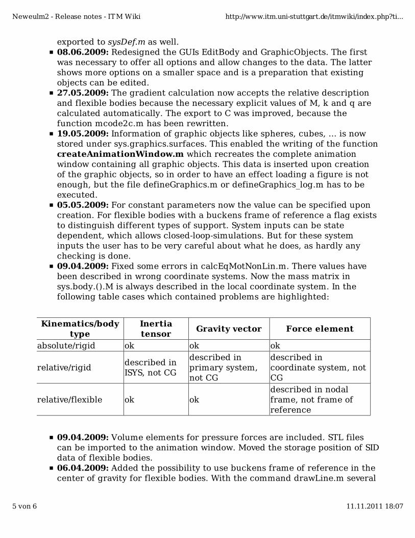
exported to sysDef.m as well.08.06.2009: Redesigned the GUIs EditBody and GraphicObjects. The firstwas necessary to offer all options and allow changes to the data. The lattershows more options on a smaller space and is a preparation that existingobjects can be edited.27.05.2009: The gradient calculation now accepts the relative descriptionand flexible bodies because the necessary explicit values of M, k and q arecalculated automatically. The export to C was improved, because thefunction mcode2c.m has been rewritten.19.05.2009: Information of graphic objects like spheres, cubes, ... is nowstored under sys.graphics.surfaces. This enabled the writing of the functioncreateAnimationWindow.m which recreates the complete animationwindow containing all graphic objects. This data is inserted upon creationof the graphic objects, so in order to have an effect loading a figure is notenough, but the file defineGraphics.m or defineGraphics_log.m has to beexecuted.05.05.2009: For constant parameters now the value can be specified uponcreation. For flexible bodies with a buckens frame of reference a flag existsto distinguish different types of support. System inputs can be statedependent, which allows closed-loop-simulations. But for these systeminputs the user has to be very careful about what he does, as hardly anychecking is done.09.04.2009: Fixed some errors in calcEqMotNonLin.m. There values havebeen described in wrong coordinate systems. Now the mass matrix insys.body.().M is always described in the local coordinate system. In thefollowing table cases which contained problems are highlighted:
Kinematics/bodytype
Inertiatensor
Gravity vector Force element
absolute/rigid ok ok ok
relative/rigiddescribed inISYS, not CG
described inprimary system,not CG
described incoordinate system, notCG
relative/flexible ok okdescribed in nodalframe, not frame ofreference
09.04.2009: Volume elements for pressure forces are included. STL filescan be imported to the animation window. Moved the storage position of SIDdata of flexible bodies.06.04.2009: Added the possibility to use buckens frame of reference in thecenter of gravity for flexible bodies. With the command drawLine.m several
Neweulm2 - Release notes - ITM Wiki http://www.itm.uni-stuttgart.de/itmwiki/index.php?ti...
5 von 6 11.11.2011 18:07
coordinate systems can be connected by cubic splines to represent flexiblebodies.26.02.2009: Changed the names and folders on the server to Neweul-M²19.02.2009: Linearization of systems with flexible bodies available on twoways: Calculate M,k,q or use partial derivatives.06.02.2009: With the 'combine' command, addition theorems of sine/cosineare available. State dependent parameters support linearization, introducedtwo force-application points.08.01.2009: Force Elements offer a nominal force, which is applied at thenominal length.22.12.2008: Instantaneous update of the animation window in the GUI.19.12.2008: System can be changed to semi-symbolic formulation, exportto m-files (independent of sys) is possible.16.12.2008: Flexible bodies are supported in the GUI.05.12.2008: Flexible bodies are implemented, no buckens frame supportedyet. Introduced the function printSystemInformation. Added the filefiniteDifferences.24.11.2008: Explicit definition of generalized coordinates wanted.11.10.2007: First available log entry.2006: Project has been started under the name of Symbs.
Retrieved from "http://www.itm.uni-stuttgart.de/itmwiki/index.php/Neweulm2_-_Release_notes"
This page was last modified 16:28, 10 November 2011.
Neweulm2 - Release notes - ITM Wiki http://www.itm.uni-stuttgart.de/itmwiki/index.php?ti...
6 von 6 11.11.2011 18:07