Embed Size (px)
Citation preview
SYMMETRY GROUP SOLUTIONS TO DIFFERENTIALEQUATIONS–A
HISTORICAL PERSPECTIVE
JACOB HARRY BURKMAN
My thanks to Professor George Wilkens for putting up with me during the lastyear while working through this project and its background material. I would alsolike to thank Professor Matt Richey of St. Olaf College, Northfield, MN for first
introducing me to the joys of differential equations.
Abstract. In this project we will be looking at Sophus Lie’sdesire (his so called idee fixe) to apply Contact Transformations(what would eventually develop into the modern idea of a Lie Al-gebra) in order to arrive at symmetries of differential equations,and thus certain solutions. Our goal—as well as Lie’s—is to de-velop a more universal method for solving differential equationsthan the familiar cook-book methods we learn in an introductoryordinary or partial differential equations class. We answer threequestions. What was the historical underpinning of Sophus Lie’stheory? How do we find the symmetry Lie algebras? How do weuse the symmetry Lie algebras to find solutions to the differentialequation? (In order to answer these questions we will need to fillin some background material and our answers will also result in anovel derivation of the “Fundamental Source Solution.”) Our sec-ond objective will be to establish a connection between solvabilityin Galois Theory and in Differential Equations. We will assume afamiliarity with certain concepts from Abstract Algebra.
Date: April 19, 2007.Master’s Plan B Project: In partial fulfillment of the the degree of Master of
Arts in Mathematics.1

2 JACOB HARRY BURKMAN
1. Algebraic Background
The desire to solve algebraic equations is something that has datedback to the time of the ancient Greeks and even before. However, likealmost everything (except somewhat superstitious theology) algebra—and mathematics—didn’t advance very far in western Europe duringthe Dark Ages. There was, however, a great deal of advancement inthe Arab world, especially in Algebra. Following a pattern similar tomany academic pursuits, mathematics came back into vogue (at leastwith some in academia) by the 18th century in Europe. This devel-opment was spurred on by the rethinking that took place during theRenaissance. Aiding this was the discovery of the work of the Arabmathematicians of the preceding centuries as well as the work of theGreeks—which had essentially been lost to the western world.
We later deal with other historical influences on Lie’s theory (c.f.Section (5)). Here, we focus on some of the algebraic material and in-fluences. We begin this with the work of Evariste Galois, culminatingin his Fundamental Theorem of Galois Theory (see [Hun80] p. 245-246).
Theorem 1. Fundamental Theorem of Galois Theory. If F isa finite dimensional Galois extension of K, then there is a one-to-onecorrespondence between the set of all intermediate fields of the exten-sion and the set of subgroups of the Galois group AutKF (given byE 7→ E ′ = AutEF ) such that:
(1) the relative dimension of two intermediate fields is equal tothe relative index of the corresponding subgroups; in particular,AutKF has order [F : K];
(2) F is Galois over every intermediate field E, but E is Galoisover K if and only if the corresponding subgroup E ′ = AutEFis normal in G = AutKF ; in this case G/E ′ is (isomorphic to)the Galois group AutKE of E over K.
In a standard course,1 this theorem receives much more attentionthan we are giving it here. However, our intention is not to cover Ab-stract Algebra, but merely to point out the connection that was soughtbetween the polynomial algebra related to Galois Theory (in partic-ular that it is possible to find some sort of correspondence between
1I would like to thank Professor Ron Brown for his encouragement and for twowonderful years of Algebra.

SYMMETRIES OF DIFFERENTIAL EQUATIONS 3
intermediate fields of a field extension K ⊂ F and the subgroups ofthe Galois group AutKF ), and the desired method of dealing with dif-ferential equations. See Section (8) for a connection between the twoideas.
An important Abstract Algebra topic is the concept of a group ac-tion. We define various results from this below (see [Hun80] ChapterII section 4).
Definition 1. An action of a group G on a set S is a function G×S →S denoted by (g, x) 7→ gx such that for all x ∈ S and g1, g2 ∈ G:
ex = x and (g1g2)x = g1(g2x)
(where e is the identity element of the group). When such an action isgiven, we say that G acts on the set S.
Now that we have a group action, the key part of this, for us, is theconcept of an orbit. (We are, at this point, not particularly interestedin the other important results, such as the Class Equation, that arisein an Abstract Algebra sense.)
Definition 2. Suppose that G is a group that acts on a set S. Thenthe relation defined on S by
x ∼ x′ ⇔ gx = x′ for some g ∈ Gis an equivalence relation. The equivalence classes of this equivalencerelation are called the orbits of G on S.
Perhaps the most important connection between Galois theory andtheory regarding symmetries of differential equations is the conceptof a solvable group (see [Hun80] p. 102). Again, we will mention itsimportance in Algebra, and realize this connection at the end of Section(7).
Definition 3. Let G be a group. The subgroup of G generated by theset aba−1b−1|a, b ∈ G is called the commutator subgroup and isdenoted by G′. Now, if we let G(1) = G′, then for each i ≥ 1, defineG(i) = (G(i−1))′ (where G(i) is called the ith derived subgroup of G).We then say that G is solvable if G(n) = 〈e〉 for some n.
Another way that solvability can be viewed is in terms of a series(see [Hun80] p 108).
Definition 4. A subnormal series of a group G is a chain of sub-groups G = G0 > G1 > · · · > Gn such that Gi+1 is normal in Gi
for 0 ≤ i ≤ n. The factors of the series are the quotient groupsGi/Gi+1. If Gn = 〈e〉 and each of the factors is abelian, the series iscalled solvable .
4 JACOB HARRY BURKMAN
Proposition 1. A group G is solvable if and only if it has a solvableseries.
The final algebraic connection we need is contained in the followingconcepts from Abstract Algebra, which we state without proof. Forproofs, see [Hun80] Chapter V, Section 9.
Definition 5. (1) LetK be a field. The Galois group of a poly-nomial f ∈ K[x] is the group AutKF , where F is a splittingfield of f over K.
(2) An extension field F of a field K is a radical extension of Kif F = K(u1, . . . , un), some power of u1 lies in K and for eachi ≥ 2, some power of ui lies in K(u1, . . . , ui−1).
(3) Let K be a field and f ∈ K[x]. The equation f(x) = 0 issolvable by radicals if there exists a radical extension F ofK and a splitting field E of f over K such that K ⊂ E ⊂ F .
Theorem 2. If F is a radical extension field of K and E is an inter-mediate field, then AutKE is a solvable group.
Theorem 3. Let K be a field and f ∈ K[x]. If f(x) is solvable byradicals, then the Galois group of f is a solvable group.
The previous theorem is half of our desired result. However, we needa technical proposition in order to get the converse. (Alternatively, wecould define a radical extension in a slightly different way. We will notpursue that here; Hungerford covers it in exercise 2 p. 309.)
Theorem 4. Let E be a finite dimensional Galois extension field of Kwith solvable Galois group AutKE. Assume that the char K does notdivide [E : K]. Then there exists a radical extension F of K, such thatK ⊂ E ⊂ F .
The following theorem is the result we really want, for it is thistheorem that has a very important parallel in the case of differentialequations (see Theorem 20).
Theorem 5. Let K be a field and f ∈ K[x] a polynomial of degreen > 0, where char K does not divide n! (which is always true whenchar K = 0). Then the equation f(x) = 0 is solvable by radicals if andonly if the Galois group of f is solvable.
SYMMETRIES OF DIFFERENTIAL EQUATIONS 5
2. Sophus Lie Background
Marius Sophus Lie was born on December 17, 1842 in Nordfjordeide,Norway to a Lutheran minster, or perhaps a farmer (see [Hel90]), Jo-hann Herman Lie. (It would not be beyond the scope of possibilitiesif he were both.) Lie attended the University of Christiania (later thecity was renamed Kristiania and then finally Oslo) studying a broadscience course. During his time at the University, Lie showed relativelylittle interest in mathematics (see [OR]). What little interest in math-ematics Lie showed was in Geometry (as we shall see, his geometricinterpretation permeated much of his work). There was, however, anexperience at the University that turned—albeit somewhat slowly—Lie’s direction in life toward our interest. Lie attended some lecturesby Ludwig Sylow in 1862-1863. The topic of these lectures was theaforementioned Galois Theory–see Section (1). However, it was notuntil considerably later (1870) after consultation with his long-timefriend and colleague Felix Klein that Lie decided it would be possibleto develop an analogue for differential equations to Galois’s theory foralgebraic equations (see [Hel90]).
We would be remiss in our duties if we failed to mention a veryinteresting event that took place in Lie’s life. Klein (a German) andLie had moved to Paris in the spring of 1870 (they had earlier beenworking in Berlin). However, in July 1870, the Franco-Prussian warbroke out. Being a German alien in France, Klein decided that itwould be safer to return to Germany; Lie also decided to go home toNorway. However (in a move that brings his geometric abilities intoquestion), Lie decided that to go from Paris to Norway, he would walkto Italy (and then presumably take a ship to Norway). The trip did notgo as Lie had planned. On the way, Lie ran into some trouble—firstsome rain, and he had a habit of taking off his clothes and puttingthem in his backpack when he walked in the rain (so he was walkingto Italy in the nude). Second, he ran into the French military (quitepossibly while walking in the nude) and they discovered in his sack(in addition to his hopefully dry clothing) letters written to Klein inGerman containing the words “lines” and “spheres” (which the Frenchinterpreted as meaning “infantry” and “artillery”). Lie was arrestedas a (insane) German spy. However, due to intervention by GastonDarboux, he was released four weeks later and returned to Norway tofinish his doctoral dissertation (see [Haw00] p. 26).

6 JACOB HARRY BURKMAN
3. Differential Equations as Usually Encountered
Before we proceed much farther, we introduce a definition and somenotation that may be helpful (note that this will apply to both ordinaryand partial differential equations) (see [Olv93] p. 96).
Definition 6. The order of a differential equation (be it ordinary orpartial) is the highest order derivative that occurs in the equation.
Notation 1. A differential equation ∆ having p independent variablesand q dependent variables is of the form ∆(x, u(n)) = 0 wherex = (x1, x2, . . . , xp), u = (u1, u2, . . . , uq) (each uj can be a function ofx), and contained in u(n) is the set of all partial derivatives of u up tothe nth order.
All students of mathematics encounter differential equations early intheir mathematical careers–usually by the second semester of Calculus.In fact, when we introduce the concept of an antiderivative, we are re-ally solving a differential equation. This introduces us to the first basicmethod of solving an ordinary differential equation—by integrating. Itdoes not (hopefully) take calculus students very long to discover thatthe differential equation by itself has an infinite number of solutions,each differing from the other by an additive constant. They also realizefairly quickly that, if a suitable number of initial conditions are added,the solution is unique. This is an example of the Uniqueness Theoremof solutions to linear differential equations, which we do not prove here.
Often the above is the extent of students’ encounters with differ-ential equations in an introductory calculus course. However, if theycontinue their studies, they begin to realize that there are a large num-ber of categories into which differential equations fit. Namely are theequations ordinary or partial; linear or non-linear; constant coefficientor variable coefficient? We initially encounter linear ordinary differen-tial equations of the first order (that is ones that contain no partialderivatives), the most general form being
(1)du
dx+ p(x)u = g(x).
We are told (see [BD97] p. 19-20) that in order to solve this equation,we need to find an integrating factor, namely
(2) µ(x) = eR
p(x)dx

SYMMETRIES OF DIFFERENTIAL EQUATIONS 7
and arrive at the general solution to Equation (1):
(3) u =
∫µ(x)g(x) dx+ c
µ(x).
Of course, anyone who has experience with integration can see thatevaluating the numerator of Equation (3) may not be the most directcalculation. However, if we adopt the convention that the differentialequation is solved once we have reduced it to quadrature, we are fin-ished with this solution. But, if we insist that we need to actuallyevaluate this antiderivative, we may be in trouble since an elementaryantiderivative of µ(x)g(x) may not exist.
Another first order equation that is “easy” to solve, especially if weagain solve only to reduction to quadrature, is a separable equation,that is, if we can write the equation in the form (see [BD97] p. 33)
(4) M(x) +N(u)du
dx= 0.
Again, Boyce (see [BD97] p. 34-35) provides a “cookbook” methodfor solving the separable equation. Provided that we can actually eval-uate the antiderivatives
∫M(x) dx and
∫N(y) dy, we have the implicit
solution
(5) H1(x) +H2(u) = c,
where c is an arbitrary constant and H1, H2 are arbitrary antideriva-tives of M,N respectively.
Example 1. 2 Solve the differential equation
(6) 2x+ u2 + 2xuu′ = 0.
Solution: Note that this equation is not linear nor is it separable(it is actually what is know as an exact equation), so the methods thatwe learned to solve linear and separable equations will not work. Weneed the method to solve exact equations. In particular, note that ifwe define a function ψ(x, u) = x2 + xu2, ψ satisfies the conditions that
2x+ u2 =∂ψ
∂x, and 2xu =
∂ψ
∂u.
Hence we can rewrite Equation (6) as
(7)∂
∂x(x2 + xu2) +
∂
∂u(x2 + xu2)
du
dx= 0.
2See [BD97] p. 83.

8 JACOB HARRY BURKMAN
But in order for this example to really have any meaning, we wouldwant u to be a function of x, so by the chain rule, we can rewriteEquation (7) as
d
dx(x2 + xu2) = 0.
which leads us to the conclusion that x2 + xu2 = c for some arbitraryconstant c is a solution of Equation (6).
Notice in the above example it was necessary to find a suitable func-tion ψ; this is the crux of solving exact differential equations. Non-linear equations such as the exact equation, can become messy (exactequations are actually very nice nonlinear equations). Perhaps this isthe reason that when we initially encounter differential equation (espe-cially nonlinear ones), the equations are very contrived examples thatfit into these various categories. We discuss several other methods andcategories below. Beside the method of solving exact equations above,another means that can possibly be used to find solutions to a nonlinearequation
M(x, u)dx+N(x, u)du = 0
is to consider integrating factors as was done in the case of linear equa-tions. This is not really our emphasis, so we continue with anotherexample of a nonlinear equation that also fits well into our box of well-behaved equations.
Definition 7. An equation of the form dudx
= f(x, u) is said to behomogeneous whenever the function f does not depend on x and useparately, but only on their ratios; that is, f is actually a function ofxu
or ux. Thus homogeneous equations are of the form du
dx= F
(ux
).
The method for solving homogeneous systems involves a change ofvariable, as we consider in the following example:
Example 2. 3 Solve the differential equation
(8)du
dx=u2 + 2xu
x2.
Solution: By isolating the denominator, we can see that we canreally write Equation (8) as
du
dx=
(ux
)2
+ 2u
x
3See [BD97] p. 91-92.

SYMMETRIES OF DIFFERENTIAL EQUATIONS 9
which shows that the equation is actually homogeneous. While it ishomogeneous, it is not linear, separable, nor exact. Thus we mustfind another method for solving the equation. Here, we consider thesubstitution u = xv, and with this, we can rewrite Equation (8) as
(9) xdv
dx= v2 + v.
Notice that Equation (9) clearly has the constant solutions v = 0,−1.These give us solutions u = 0,−x of Equation (8). Therefore let usassume that v 6= 0, v 6= −1, in which case, we can rewrite Equation (9)using partial fractions as
dx
x=
(1
v− 1
v + 1
)dv.
This is separable, so we solve it by integrating, arriving at
ln |x|+ ln |c| = ln |v| − ln |v + 1|where c is the arbitrary constant of integration. Using rules of loga-rithms and by taking the exponential of each side, we arrive at
cx =v
v + 1.
But, recall that v = ux, so we get the implicit solution
cx =ux
ux
+ 1=
u
u+ x
to Equation (8). However, the above is actually nice enough that wecan solve for u, namely the general solution
(10) u =cx2
1− cx.
Just as a point of reference, notice that the solutions u = 0 andu = −x are included in Equation (10); the former when c is chosen tobe 0, and the latter as a limit when c→ ±∞.
We now do a foray into partial differential equations. Very often(as is the case in Bleecker & Csordas [BC96]),4 the first named partialdifferential equation that we see is the heat equation: ut = uxx.
5 ForBleecker & Csordas this happens at the beginning of Chapter 3. Af-ter a slight physical interpretation introduction to the heat equation
4My thanks to Professor Bleecker for agreeing to be on my committee, and forProfessor Csordas for his invigorating teaching.
5If one goes precisely off what Bleecker & Csordas have as the heat equation,there is a positive parameter k such that ut = kuxx. By a change of coordinates,we assume without loss of generality that k = 1 in our calculations.

10 JACOB HARRY BURKMAN
(where the authors actually derive the heat equation from elementaryprinciples), we, the readers, are told that the function
u(x, t) =1√4πt
e−x2
4t , t > 0,−∞ < x <∞
is a special solution to the heat equation called the “FundamentalSource Solution” (see [BC96] p. 124). The authors, and presumablythe readers, then show that this is a solution by using logarithmic dif-ferentiation. Bleecker & Csordas later derive (see [BC96] p. 460-461)the “Fundamental Source Solution” using the method of Fourier trans-forms.6 We also derive this solution in Section (5) using the alternativemethod of symmetry groups.
Following this, Bleecker & Csordas introduce us to what is presum-ably (at least from reading them) the most common analytical way ofsolving partial differential equations, and that is to use the method ofSeparation of Variables by seeking product solutions. In separation ofvariables we seek solutions of the form u(x, t) = X(x)T (t). Applyingthis to the heat equation, we get the result that
T ′(t)
T (t)=X ′′(x)
X(x).
But, since the left hand side is a function of t and the right handside is a function of x, the only way this can happen is if they are aconstant, c. We are then left with two ordinary differential equations:T ′(t)−cT (t) = 0, andX ′′(x)−cX(x) = 0, which we solve using ordinarydifferential equation methods, giving us the following solutions.
(1) If c = −λ2 < 0, then the product solution is of the form:
u(x, t) = e−λ2t(c1 sin(λx) + c2 cos(λx)
).
(2) If c = λ2 > 0, then the product solution is of the form:
u(x, t) = eλ2t(c1eλx + c2e
−λx).
(3) If c = 0, then the product solution is of the form:
u(x, t) = c1x+ c2.
6In Exercise 13 p. 139, Bleecker & Csordas also describe a way by which the“Fundamental Source Solution” can be derived using a probabilistic method similarto a random walk. There are additional means by which this can be derived; someare very elementary. However, our goal here is neither to discover all means bywhich one can derive the “Fundamental Source Solution,” nor the easiest.

SYMMETRIES OF DIFFERENTIAL EQUATIONS 11
As the reader progresses through Bleecker & Csordas, we begin tosee the work of Fourier applied to partial differential equations. In thisprocess, one combines the use of product solutions and the superposi-tion principle (that a linear combination of solutions are solutions) inorder to arrive at solutions that can be represented by a finite sum ofproduct solutions. In most applications, we really want to know whathappens when there are certain specified initial conditions. In the casepreviously mentioned, the initial conditions of the finite sum of productsolutions are trigonometric polynomials. Now suppose that we have asan initial condition a function f that is continuous and piecewise C1.Fourier’s goal was to show that f could be approximated by a sum,which need not necessarily finite, of these trigonometric polynomials.In the case that it is not finite, we call it a Fourier series. We can thenshow that a sequence of solutions coming from partial sums convergesto an actual solution (this is done merely formally). As we proceed intothe later part of Bleecker & Csordas, we get to perhaps the most directanalytical means to solve partial differential equations and that is touse Fourier transforms (as mentioned earlier, it is by means of Fouriertransforms that one can derive the “Fundamental Source Solution”).

12 JACOB HARRY BURKMAN
4. Lie Groups and Differential Geometry
While it is not our emphasis here, we need to do a slight overview ofsome topics in Differential Geometry and Lie Groups, since these willbe important to our understanding of the culmination of Lie’s inter-pretation of how to analyze solution spaces for differential equations.The basic structure is a manifold (see [Olv93] p. 3).
Definition 8. An m-dimensional smooth manifold is a nonemptyset M , together with a countable collection of subsets Uα ⊂M , calledcoordinate charts, and one-to-one functions χα : Uα → Vα onto openconnected subsets Vα ⊂ Rm, called local coordinate maps which sat-isfy the following properties.
(1) The coordinate charts cover M ; that is⋃α
Uα = M.
(2) On the overlap of any pair of coordinate charts Uα ∩ Uβ, thecomposite map
χβ χ−1α : χα(Uα ∩ Uβ)→ χβ(Uα ∩ Uβ)
is a smooth (meaning infinitely differentiable) function.(3) If x ∈ Uα, y ∈ Uβ are distinct points in M , then there exist
open subsets W ⊂ Vα, Y ⊂ Vβ, with χα(x) ∈ W,χβ(y) ∈ Y ,satisfying
χ−1α (W ) ∩ χ−1
β (Y ) = ∅.
Once we have manifolds (which we will, by means of the coordinatemaps, consider to be essentially some subset of Euclidean space), wecan define (see [Olv93] p. 7-8) the following.
Definition 9. If M and N are smooth manifolds, a map F : M → Nis said to be smooth if its local coordinate expression is a smooth mapin every coordinate chart.
Definition 10. Let F : M → N be a smooth mapping from an m-dimensional manifold M to an n-dimensional manifold N . The rankof F at a point x ∈ M is the rank of the n × m Jacobian matrix(∂F i/∂xj) at x, where y = F (x) is expressed in any local coordinatesnear x. The mapping F is of maximal rank on a subset S ⊂ M if
SYMMETRIES OF DIFFERENTIAL EQUATIONS 13
for each x ∈ S, the rank of F is as large as possible (i.e. the minimumof m and n).
Note that the rank mentioned in Definition 10 is independent of thechoice of coordinates on the manifolds.
We now move on to the important concept of vectors in DifferentialGeometry. Connected with each point x ∈M are tangent vectors (ba-sically in the usual calculus sense). We consider these in the followingdefinitions.
Definition 11. The collection of all tangent vectors to all possiblecurves passing through a given point x ∈ M is called the tangentspace to M at x.
Notation 2. We denote the tangent space to M at x by TM |x.
Note that if M is an m-dimensional manifold, then TM |x is an m-dimensional vector space with basis ∂/∂x1, . . . ∂/∂xm in the localcoordinates (x1, . . . , xm).
Definition 12. The set
TM :=⋃
x∈M
TM |x
is the tangent bundle of M . This set has a natural manifold struc-ture of dimension 2m.
One of the most important concepts that we will need is that of avector field.
Definition 13. A vector field v on M is a function that assignsa tangent vector v|x ∈ TM |x to each point x ∈ M , where v|x variessmoothly from point to point.
We will follow Olver’s (see [Olv93] p. 26) notation for a vector field,namely if we have local coordinates (x1, x2, . . . xm), the vector field hasthe form
v|x = ξ1(x)∂
∂x1+ ξ2(x)
∂
∂x2+ · · ·+ ξm(x)
∂
∂xm
where each ξi(x) is a smooth function of x (and we are using super-scripts as indices).
Proposition 2. Vector fields are first order linear differential operatorson smooth functions which operate by the action
(v · f)(x) = ξ1 ∂f
∂x1(x) + · · ·+ ξm ∂f
∂xm(x)
14 JACOB HARRY BURKMAN
for any smooth function f : M → R.
One of the primary operations on vector fields that we will use isknown as the Lie Bracket.
Definition 14. If v,w are vector fields onM , then their Lie Bracket ,which we denote by [v,w], is the unique vector field satisfying
[v,w] · (f) = v(w · (f)
)−w
(v · (f)
)for all smooth functions f : M → R.
Proposition 3. The Lie Bracket satisfies the following properties.
(1) Bilinearity: If v1,v2,w1,w2 are vector fields and c1, c2, c3, c4are constants, then
[c1v1+c2v2, c3w1+c4w2] = c1c3[v1,w1]+c1c4[v1,w2]+c2c3[v2,w1]+c2c4[v2,w2].
(2) Skew-Symmetry: If v,w are vector fields, then
[v,w] = −[w,v].
(3) Jacobi Identity: If v,w,u are vector fields, then[u, [v,w]
]+
[w, [u,v]
]+
[v, [w,u]
]= 0.
Now suppose that we have two vector fields, a(x, y) ∂∂x
and b(x, y) ∂∂y
,
then we can find their Lie Bracket by
(11)[a(x, y)
∂
∂x, b(x, y)
∂
∂y
]= a(x, y)
∂
∂xb(x, y)
∂
∂y− b(x, y) ∂
∂ya(x, y)
∂
∂x.
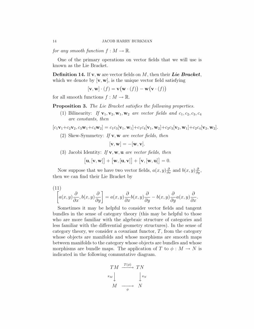
Sometimes it may be helpful to consider vector fields and tangentbundles in the sense of category theory (this may be helpful to thosewho are more familiar with the algebraic structure of categories andless familiar with the differential geometry structures). In the sense ofcategory theory, we consider a covariant functor, T , from the categorywhose objects are manifolds and whose morphisms are smooth mapsbetween manifolds to the category whose objects are bundles and whosemorphisms are bundle maps. The application of T to φ : M → N isindicated in the following commutative diagram.
TMT (φ)−−−→ TN
πM
y yπN
M −−−→φ
N

SYMMETRIES OF DIFFERENTIAL EQUATIONS 15
We can then define a vector field to be a special function, v : M →TM such that the πM v is the identity map on M . (We may also call va section of the bundle.) Furthermore, the map T (φ) is the differentialof the map φ.
One important theorem in vector fields and coordinates is what isknown as the “Flow Box Theorem” (see [Olv93] p. 30).
Theorem 6. Flow Box Theorem. Let
v|x = ξ1(x)∂
∂x1+ ξ2(x)
∂
∂x2+ · · ·+ ξn(x)
∂
∂xn
be a vector field. Let m ∈ M (where M , of course, is a manifold)such that v|x(m) 6= 0. Then there is a local coordinate chart y =(y1, y2, . . . , yn) at m such that in these coordinates, we have thatv|y = ∂
∂y1 .
What this theorem does is enable us to make a suitable change ofcoordinates and make the vector field much easier to deal with; ineffect, we can straighten out the flow. (We have not defined flow here,but one can essentially think of it as the path a particle would takethrough a vector field as encountered in an introductory differentialequations course.)
Now that we have at least some definitions available we can finallydefine a Lie Group (see [Olv93] p. 15).
Definition 15. An r-parameter Lie group is a group G which alsocarries the structure of an r-dimensional manifold in such a way asboth the group operation
m : G×G→ G, m(g, h) = g · h, g, h ∈ G,and the inversion
i : G→ G, i(g) = g−1, g ∈ G,are smooth maps between manifolds.
Almost all properties we will be interested in are actually local.Hence we are usually interested only in a local Lie Group (see [Olv93]p. 18).
Definition 16. An r-parameter local Lie group consists of opensubsets V0 ⊂ V ⊂ Rr containing the origin 0, and smooth maps
m : V × V → Rr,

16 JACOB HARRY BURKMAN
defining the group operation, and
i : V0 → V
defining the group inversion which has the following properties.
(1) Associativity: If x, y, z ∈ V , and m(x, y),m(y, z) ∈ V , then
m(x,m(y, z)
)= m
(m(x, y), z
).
(2) Identity Element: For all x ∈ V , m(0, x) = x = m(x, 0).(3) Inverses: For each x ∈ V0, m
(x, i(x)
)= 0 = m
(i(x), x
).
The previous two definitions have to do with a modern interpreta-tion. However when Lie would consider a group, he actually wouldbe considering what we could call a Lie Algebra, not what has todaybecome known as a Lie Group. We will adopt the more modern termi-nology.
Throughout this, let G be a Lie Group with right multiplication mapRg : G→ G defined by Rg(h) = hg for all h ∈ G. We then say that vis a right invariant vector field if T (Rg) v Rg−1 = v for all g ∈ G.
Proposition 4. The Lie Bracket of two right invariant vector fields isright invariant.
The proof of this proposition follows directly from appropriate ap-plications of definitions. But, once we have it, we can define a LieAlgebra.
Definition 17. A Lie algebra is a vector space g together with theoperation of the Lie Bracket (c.f. Definition 14) satisfying conditions1, 2, and 3 of Proposition 3.
An example of a Lie Algebra is the vector space of all right invariantvector fields on G with the operation of the Lie Bracket. One thingto note is that we often do not consider g as we have defined it. Theway we consider the Lie Algebra is actually that g = TG|e, that is, itis the tangent space to the identity. One considers the set of vectorfields to be the infinitesimal generators of a Lie Algebra, so supposethat v1, . . . ,vr forms a basis for g. Then by closure, [vi,vj] ⊂ g.
Definition 18. From this, we arrive at some very important constants,ckij, i, j, k = 1, . . . , r, the so called structure constants. They aredefined by the relationship
[vi,vj] =r∑
k=1
ckijvk, i, j = 1, . . . , r.
SYMMETRIES OF DIFFERENTIAL EQUATIONS 17
Proposition 5. From the properties of the Lie Bracket, we can clearlysee that the structure constants also satisfy the following properties.
(1) Skew Symmetry: ckij = −ckji, and(2) Jacobi Identity:
r∑k=1
(ckijc
mkl + cklic
mkj + ckjlc
mki
)= 0 m = 1, . . . , r.
Definition 19. A Lie Algebra g is a abelian if [v,w] = 0 for everyv,w ∈ g.
Proposition 6. A Lie subgroup H of a Lie group G is normal if anonly if its Lie algebra h ⊂ g has the property that [v,w] ∈ h wheneverv ∈ g and w ∈ h; in other words, it satisfies the ideal property.
In fact, we can actually completely reduce our study to any one ofthe following: a Lie Group G, a Lie Algebra g, or a set of structureconstants. For instance a set of constants satisfy the results of Propo-sition 5 if and only if they are the structure constants for some LieAlgebra g. Similarly given any Lie Group, we can find a Lie Algebra,and given any Lie Algebra, h,we can find a Lie Group that has h as itsLie Algebra.7
Before we start talking about how Lie saw differential equations, weneed more concepts. The first of these is prolongation. While prolonga-tion is actually something that can occur with diffeomorphisms, vectorfields, group actions and flows, we will, for the sake of some brevity,primarily focus on the prolongation of a vector field. Since a vectorfield is really a function, we first introduce the idea of the prolongationof a function. We then extend this to the idea of the prolongation ofa vector field. However, we need to build up some background beforewe can get to prolongation. Here, we consider the manifold to simplybe Euclidean space.
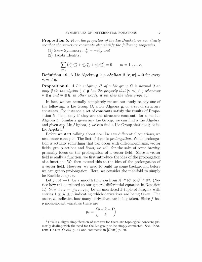
Let f : X → U be a smooth function from X ∼= Rp to U ∼= Rq. (No-tice how this is related to our general differential equation in Notation1.) Now let J = (j1, . . . , jk) be an unordered k-tuple of integers withentries 1 ≤ jk ≤ p indicating which derivatives are being taken. Theorder, k, indicates how many derivatives are being taken. Since f hasp independent variables there are
pk ≡(p+ k − 1
k
)7This is a slight simplification of matters for there are topological concerns pri-
marily dealing with the need for the Lie group to be simply-connected. See Theo-rem 1.54 in [Olv93] p. 47 and comments in [Olv93] p. 50.

18 JACOB HARRY BURKMAN
different kth order partial derivatives of f .
Notation 3. We denote these derivatives by
uαJ = ∂Jf
α(x) =∂kfα(x)
∂xj1∂xj2 · · · ∂xjk
where α = 1, . . . , q.
Note that there are q · pk such derivatives.
Notation 4. Let us denote the Euclidean space Rq·pk by Uk.
Furthermore, let us endow the space Uk with coordinates uαJ which
represent the derivatives in Notation 3.
Notation 5. Set U (n) := U×U1×· · ·×Un to be the cartesian productspace. The coordinates of the space U (n) represent all the derivativesof functions u = f(x) of all orders from 0 to n.
Note that U (n) is a Euclidean space with dimension q(
p+nn
)≡ qp(n).
Notation 6. We will denote by u(n) a typical point in the space U (n);the components of u(n) are the aforementioned uα
J where 0 ≤ k ≤n, 1 ≤ α ≤ q.
Definition 20. Let u = f(x) be a smooth function from X to U .Then there is an induced function, u(n) = pr(n) f(x), called the nth
prolongation of f , which is defined by the equations uαJ = ∂Jf
α(x).
Example 3. Suppose we have the heat equation
(12) ut − uxx = 0.
Here, note that there are two independent variables, x, t, one depen-dent variable, u, so we have the underlying space X×U ∼= R2×R withcoordinates (x, t, u). Since Equation (12) contains a second order par-tial derivative, we will want to consider the prolongation to the 2-jet,namely to the setX×U (2), which has coordinates (x, t, u, ux, ut, uxx, uxt,utt). We return to this example later.
Definition 21. The set X × U (n) is the nth order jet space of theunderlying space X × U .
In considering prolongations of functions, the key idea is to identifythe function u with its graph in X×U . We can now generalize the ideato that of a vector field, v. Note that a vector field will operate on thespace X × U ∼= M , and it will prolong up to a function operating onX × U (n) ∼= M (n).

SYMMETRIES OF DIFFERENTIAL EQUATIONS 19
M (n) pr(n) v−−−−→ TM (n)
π
y yT (π)
M −−−→v
TM
The prolongation is a lifting of the vector field in the sense that theabove diagram commutes, i.e. v π = T (π) pr(n) v.
Here we shall calculate a simple prolongation of a vector field. (Wedo another calculation in Example 6, where there are more independentvariables.)
Example 4. Find the 1st prolongation of the most general vector fieldover a X × U where there is only one independent variable, in otherwords, find pr(1) v where
v = ξ(x, u)∂
∂x+ φ(x, u)
∂
∂u.
To solve this, first note that the prolongation will be a vector field
pr(1) v = ξ(x, u)∂
∂x+ φ(x, u)
∂
∂u+ φx(x, u, ux)
∂
∂ux
.
By the lifting and covering mentioned above, all we need to do isto find the coefficient function φx (we assume that we are given thefunctions ξ and φ). For notation, we will follow Olver and have thesuperscripts of the function φ match with the basis element of thecoordinate map. We can solve this several ways. Here we find theprolongation using Lie Derivatives and the invariance of a certain 1-form. (We use an alternate method in Example 6.)
Definition 22. Let v be a vector field on M with flow ϕε and σ avector field or differential form defined on M . The Lie Derivative ofσ with respect to v is the object whose value at x ∈M is
(Lvσ)|x = limε→0
ϕ∗ε(σ|ϕε(x))− σ|xε
.
This definition is even more ungainly than the corresponding def-inition for regular derivatives which nearly every Calculus 1 studenthas difficulty grasping. And, as in the case of Calculus 1, where soonthe student learns the various rules for differentiating a function of areal variable, we skip ahead to some important properties of the LieDerivative.
(1) The Lie Derivative is linear over the reals (as any good deriva-tive should be).
20 JACOB HARRY BURKMAN
(2) If f is a function (note that a function is a differential form),then Lvf = v · f ; that is, apply the vector field to the functionf .
(3) If df is the differential of a function f , then Lvdf = d(Lvf) =d(v · f).
(4) The Lie derivative obeys the product rule.
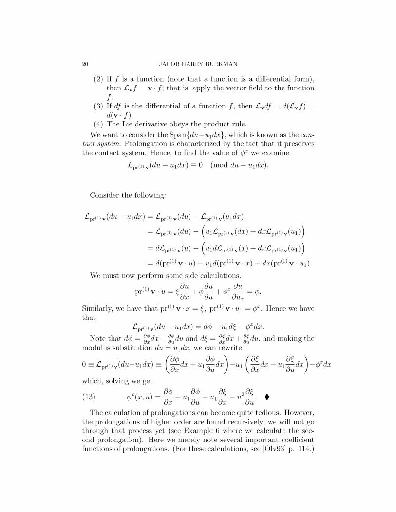
We want to consider the Spandu−u1dx, which is known as the con-tact system. Prolongation is characterized by the fact that it preservesthe contact system. Hence, to find the value of φx we examine
Lpr(1) v(du− u1dx) ≡ 0 (mod du− u1dx).
Consider the following:
Lpr(1) v(du− u1dx) = Lpr(1) v(du)− Lpr(1) v(u1dx)
= Lpr(1) v(du)−(u1Lpr(1) v(dx) + dxLpr(1) v(u1)
)= dLpr(1) v(u)−
(u1dLpr(1) v(x) + dxLpr(1) v(u1)
)= d(pr(1) v · u)− u1d(pr(1) v · x)− dx(pr(1) v · u1).
We must now perform some side calculations.
pr(1) v · u = ξ∂u
∂x+ φ
∂u
∂u+ φx ∂u
∂ux
= φ.
Similarly, we have that pr(1) v · x = ξ, pr(1) v · u1 = φx. Hence we havethat
Lpr(1) v(du− u1dx) = dφ− u1dξ − φxdx.
Note that dφ = ∂φ∂xdx+ ∂φ
∂udu and dξ = ∂ξ
∂xdx+ ∂ξ
∂udu, and making the
modulus substitution du = u1dx, we can rewrite
0 ≡ Lpr(1) v(du−u1dx) ≡(∂φ
∂xdx+ u1
∂φ
∂udx
)−u1
(∂ξ
∂xdx+ u1
∂ξ
∂udx
)−φxdx
which, solving we get
(13) φx(x, u) =∂φ
∂x+ u1
∂φ
∂u− u1
∂ξ
∂x− u2
1
∂ξ
∂u.
The calculation of prolongations can become quite tedious. However,the prolongations of higher order are found recursively; we will not gothrough that process yet (see Example 6 where we calculate the sec-ond prolongation). Here we merely note several important coefficientfunctions of prolongations. (For these calculations, see [Olv93] p. 114.)

SYMMETRIES OF DIFFERENTIAL EQUATIONS 21
Here we look at the case where there are two independent variables,namely we have a vector field over X × U ∼= R2 × R which has thegeneral form
(14) v = ξ(x, t, u)∂
∂x+ τ(x, t, u)
∂
∂t+ φ(x, t, u)
∂
∂u.
Recalling what happens when we make prolongations, we can seedirectly that (here, for the sake of space, we remove the argumentsfrom the coefficient functions, which is a practice we will continue tofollow provided it does not cause confusion)
(15) pr(1) v = ξ∂
∂x+ τ
∂
∂t+ φ
∂
∂u+ φx ∂
∂ux
+ φt ∂
∂ut
and that
(16)
pr(2) v = ξ∂
∂x+τ
∂
∂t+φ
∂
∂u+φx ∂
∂ux
+φt ∂
∂ut
+φxx ∂
∂uxx
+φxt ∂
∂uxt
+φtt ∂
∂utt
.
In Equations (15) and (16), we have that
(17) φx = φx + (φu − ξx)ux − τxut − ξuu2x − τuuxut,
(18) φt = φt − ξtux + (φu − τt)ut − ξuuxut − τuu2t ,
(19)
φxx = φxx +(2φxu−ξxx)ux−τxxut +(φuu−2ξxx)u2x−2τxuuxut−ξuuu
3x
− τuuu2xut + (φu− 2ξx)uxx− 2τxuxt− 3ξuuxuxx− τuutuxx− 2τuuxuxt.
We will return to these when we discuss the heat equation.

22 JACOB HARRY BURKMAN
5. Sophus Lie and Differential Equations
Recall from Section (2) that Sophus Lie was at heart a geometer,and it was through this lens that he viewed much of his work. Wehad previously mentioned (again see Section (2)) that Lie had a closeassociation with the German mathematician Felix Klein (who was astudent of Julius Plucker), and it was through studies of Plucker’s linegeometry that Klein and Lie’s association began.8 While it is not com-pletely relevant to the topic, we will spend a little bit of time dealingwith this initial topic of Klein and Lie’s since we see a similar approachlater in Lie’s approach to differential equations.
Let ∆ denote a fixed tetrahedron, with faces determined by planesπ1, π2, π3, π4. Then we clearly have that each ` in P3(C) meets ∆ infour places. A tetrahedral line complex T is the set of lines ` for whichthe cross ratio of these points is the same.
Notation 7. Let B denote the totality of all projective transformationsof the space that fixes the vertices of the tetrahedron ∆. We essentiallythink of the elements of B as coordinate changes.
What was unique (and for our sake informative) about Lie’s ap-proach to these tetrahedral line complexes was (see [Haw00] p. 6) thatto him a tetrahedral complex was the orbit (in the sense of a groupaction) of some fixed line under the transformations of B. For us, thisis informative since he tried to understand differential equations in asimilar way.
Lie’s study of differential equations in this sense became his idee fixe.To get into this, let us suppose that we have a point p in our space.From this point p, we can arrive at the complex cone with vertex p,which we will denote by C(p). This is the set of all lines of T that passthrough the point p.
Problem: Determine all surfaces S with the property that at eachpoint p ∈ S, the cone C(p) touches S at p. In other words, the tangentplane to S meets the cone C(p) in exactly one straight line.
8One important connection was Klein’s Erlanger Programm which “consisted inimplicitly regarding all the geometries or geometrical modes of treatment...[as being]completely determined by specifying a manifold of elements and a distinguishedset of transformations acting on the elements of the manifold and defining thepermissible geometrical operations” (see [Haw00] p. 35). One then considers thoseelements of the manifold that are invariant under the operations.

SYMMETRIES OF DIFFERENTIAL EQUATIONS 23
Since the geometrical condition on S can be translated into an equa-tion of the form
(20) f(x, y, z, p, q) = 0, p =∂z
∂x, q =
∂z
∂y,
the solution to this problem (according to Lie) (see [Haw00] p. 21-22),amounts to solving a first order partial differential equation. We canclearly note that geometrically any T ∈ B will take one solution surfaceinto another; Lie would later describe this as saying that the differentialequation admits the transformations of B. Lie’s actual solution to theproblem involved the maps
X = log x, Y = log y, Z = log z.
But since the differential equation noted admits all elements of B, Lieconcluded that the differential equation could actually be reduced toone of the form f(p, q) = 0 which could be solved directly. His reasonfor this is contained in Theorem 7.
When Lie shared this result with Klein (who apparently had morealgebraic knowledge or possibly interest), he noticed that there was ananalogy between Lie’s method of integrating differential equations ad-mitting a 3-parameter group of commuting transformations (as in theproblem above) and in Abel’s work on abelian polynomial equations.Recall that in polynomial Galois theory the elements of the Galoisgroup permute the roots of the associated polynomial; that is, theytake solutions into solutions. The above problem and Lie’s solution toit seemed to indicate a similar result may happen here: knowing some-thing about the group admitted yields information about the solution.
We can see another example of this in the case of Equation (8), thehomogeneous equation example mentioned in Section (3), which admitsthe 1-parameter group of commuting transformations x′ = ax and y′ =ay. (That is, the homogeneous equation admits a scaling symmetry—see Example 7.) Lie felt this was the reason we could solve Equation(8) by using a change of variables. With these in hand, we see thatLie felt that “knowledge of transformations, ‘finite’ or infinitesimal,admitted by a differential equation was the true basis for its solutionor at least for its reduction to a simpler equation. . . . It thus seemedplausible that a bona fide theory of differential equations admittingknown, commuting, infinitesimal transformations could be developedthat would serve a function analogous to that served by Galois’s theoryfor polynomial equations.”9 To this end, Lie came up with the followingtheorem (see [Haw00] p. 24).
9See [Haw00] p. 24.

24 JACOB HARRY BURKMAN
Theorem 7. Lie, ca. 1870.
(1) If f(x, y, z, p, q) = 0 admits three commuting infinitesimal pro-jective transformations, then it can be transformed intoF (P,Q) = 0.
(2) If f(x, y, z, p, q) = 0 admits two commuting infinitesimal pro-jective transformations, then it can be transformed intoF (Z, P,Q) = 0.
(3) If f(x, y, z, p, q) = 0 admits one commuting infinitesimal projec-tive transformation, then it can be transformed into an equationwithout the third coordinate F (X, Y, P,Q) = 0.
As is the case with much of Lie’s work, his proof to this theorem wasnot very rigorous (such as obtaining an unlimited number of differen-tial equations for which it applied). The theorem also has a number ofproblems with its lack of generality. Lie’s idee fixe was that the resultsof this theorem could be expanded and developed on a far greater scaleand generality than implied in this theorem. However, because of thevastness of differential equations (compared to polynomial equations)the full extent of Lie’s idee fixe has yet to be realized. But Lie’s interestin differential equations was kindled, and many mathematicians sinceLie have attempted to expand on his idee fixe.
As we saw above, Lie became fascinated with differential equations.We would like to take a little bit of time to go over other motivationsof his as well as knowledge that he would have had of differential equa-tions. We had previously mentioned the geometric impetus given toLie by Felix Klein. Much of Lie’s formative knowledge on differentialequations came from an essay written by V. G. Imschenetsky in 1869.Imschenetsky was inspired by the work of one of the greatest mathe-maticians of all time, Carl Gustav Jacob Jacobi. Jacobi, who did hiswork primarily in the 1830’s, did not publish many of his results, forthe results were published posthumously by Clebsch in the 1860’s. Itwas Jacobi, “the quintessential analyst, [who] provided the analyticalframework for Lie’s geometrical ideas.”10 As a basis for Jacobi’s (andhence Lie’s) work, we start with a result of Lagrange (see [Haw00] p.45) that is essentially the Flow Box Theorem (c.f. Theorem 6).
Theorem 8. Lagrange’s Theorem. The problem of determining allsolutions f = f(x1, . . . , xn) to a linear homogeneous equation
ξ1∂f
∂x1
+ · · ·+ ξn∂f
∂xn
= 0, ξi = ξi(x1, . . . , xn)
10See [Haw00] p. 46.
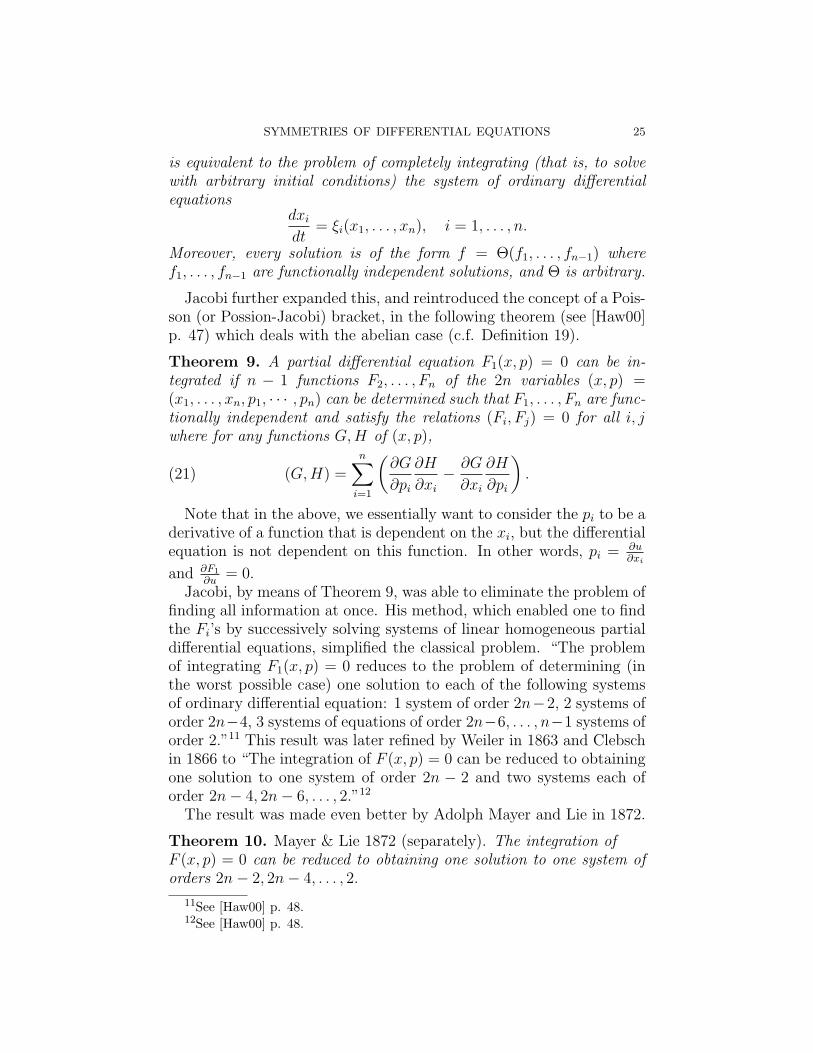
SYMMETRIES OF DIFFERENTIAL EQUATIONS 25
is equivalent to the problem of completely integrating (that is, to solvewith arbitrary initial conditions) the system of ordinary differentialequations
dxi
dt= ξi(x1, . . . , xn), i = 1, . . . , n.
Moreover, every solution is of the form f = Θ(f1, . . . , fn−1) wheref1, . . . , fn−1 are functionally independent solutions, and Θ is arbitrary.
Jacobi further expanded this, and reintroduced the concept of a Pois-son (or Possion-Jacobi) bracket, in the following theorem (see [Haw00]p. 47) which deals with the abelian case (c.f. Definition 19).
Theorem 9. A partial differential equation F1(x, p) = 0 can be in-tegrated if n − 1 functions F2, . . . , Fn of the 2n variables (x, p) =(x1, . . . , xn, p1, · · · , pn) can be determined such that F1, . . . , Fn are func-tionally independent and satisfy the relations (Fi, Fj) = 0 for all i, jwhere for any functions G,H of (x, p),
(21) (G,H) =n∑
i=1
(∂G
∂pi
∂H
∂xi
− ∂G
∂xi
∂H
∂pi
).
Note that in the above, we essentially want to consider the pi to be aderivative of a function that is dependent on the xi, but the differentialequation is not dependent on this function. In other words, pi = ∂u
∂xi
and ∂F1
∂u= 0.
Jacobi, by means of Theorem 9, was able to eliminate the problem offinding all information at once. His method, which enabled one to findthe Fi’s by successively solving systems of linear homogeneous partialdifferential equations, simplified the classical problem. “The problemof integrating F1(x, p) = 0 reduces to the problem of determining (inthe worst possible case) one solution to each of the following systemsof ordinary differential equation: 1 system of order 2n−2, 2 systems oforder 2n−4, 3 systems of equations of order 2n−6, . . . , n−1 systems oforder 2.”11 This result was later refined by Weiler in 1863 and Clebschin 1866 to “The integration of F (x, p) = 0 can be reduced to obtainingone solution to one system of order 2n − 2 and two systems each oforder 2n− 4, 2n− 6, . . . , 2.”12
The result was made even better by Adolph Mayer and Lie in 1872.
Theorem 10. Mayer & Lie 1872 (separately). The integration ofF (x, p) = 0 can be reduced to obtaining one solution to one system oforders 2n− 2, 2n− 4, . . . , 2.
11See [Haw00] p. 48.12See [Haw00] p. 48.

26 JACOB HARRY BURKMAN
Adolph Mayer (whose specialty was in differential equations) wasmuch more of an analyst than Lie. Mayer arrived at the above resultusing analytical means; Lie, by his somewhat typically inspirationalmeans, arrived at the result geometrically. It was, however, throughMayer that Lie gained the Jacobian analytical view of differential equa-tions.
The above mentioned results were critical in Lie’s realization of hisidee fixe. These theorems, particularly the Mayer/Lie Theorem, mademore specific the manner in which knowledge that a differential equa-tion admits a group of transformations should yield information aboutits integration by translating into the number and order of systemsof ordinary differential equations needed to integrate the original par-tial differential equation. In this sense, we are finally beginning to seethe connection between the way Lie saw differential equations and theresults for Galois theory of polynomials. “The system of ordinary dif-ferential equations played somewhat the role of the auxiliary polynomialequations associated to the composition series of the Galois group of apolynomial equation and utilized to analyze its algebraic resolution.”13
Lie needed a little bit more before he could really do this—he neededto translate group related information into auxiliary systems.
Jacobi, as mentioned, failed to publish his later results (largely dueto failing health), and also failed to provide justification for his results.Many did not believe his claims regarding the general case of Theo-rem 9—it is a generalization since it removes the abelian condition—resulting in what is known as “Jacobi’s Problem” (see [Haw00] p. 51).
Jacobi’s Problem. Suppose that f = F1, . . . , Fr are r functionallyindependent solutions to (F1, f) = 0 with the property that the brack-eting produces no more solutions in the sense that for all i, j, (Fi, Fj)is functionally dependent upon F1, . . . , Fr, so that functions Ωij of rvariables exist for which
(Fi, Fj) = Ωij(F1, . . . , Fr), i, j = 1, . . . , r.
How does knowledge of F1, . . . , Fr simplify the problem of solvingF1(x, p) = 0?
While several mathematicians between Jacobi and Lie had dealt withthis problem, it was Lie who “was the first to tackle the general prob-lem, inspired by the fact that for him, it was an expression of his ideefixe.”14 In fact, we can even express the problem in terms of the idee
13See [Haw00] p. 50.14See [Haw00] p. 51.

SYMMETRIES OF DIFFERENTIAL EQUATIONS 27
fixe: “Given that the partial differential equation F1(x, p) = 0 admitsthe group gF , how does knowledge of gF simplify the problem of solv-ing F1(x, p) = 0?”15
In realizing a solution similar to what Lie would have envisioned, weneed several key theorems and definitions (see [Olv93] p. 93, 100-101).
Definition 23. Let S be a system of differential equations. A sym-metry group of the system S is a local group of transformations Gacting on an open subset M of the space of independent and dependentvariables for the system with the property that whenever u = f(x) is asolution of S, and whenever g · f is defined for g ∈ G, then u = g · f(x)is also a solution of the system.
Notation 8. Let ∆(x, u(n)) = 0 be an nth order differential equation.Denote by S∆ the subvariety of X × U (n) that is ∆−1(0).
Theorem 11. Let M be an open subset of X × U and suppose that∆(x, u(n)) = 0 is an nth order system of differential equations definedover M , with corresponding sub-variety S∆ ⊂ M (n). Suppose that Gis a local group of transformations acting on M whose prolongationleaves S∆ invariant, meaning that whenever (x, u(n)) ∈ S∆, we havepr(n) g · (x, u(n)) ∈ S∆ for all g ∈ G such that this is defined. Then G isa symmetry group of the system of differential equations in the senseof definition (23).
The theorem that we will primarily use is the following (usually withl = 1) (see [Olv93] p. 104).
Theorem 12. Suppose that ∆v(x, u(n)) = 0 for v = 1, . . . , l is a system
of differential equations of maximal rank defined over M ⊂ X × U . IfG is a local group of transformations acting on M andpr(n) v
(∆v(x, u
(n)))
= 0, v = 1, . . . , l whenever ∆v(x, u(n)) = 0 for
every infinitesimal generator v of G, then G is a symmetry group ofthe system.
We can also interpret Theorem 12 in terms of the Lie algebra.
Theorem 13. G is a symmetry group for ∆ if and only if g(n) istangent to S∆.
15See [Haw00] p. 59.

28 JACOB HARRY BURKMAN
6. The Heat and Wave Equations
Example 5. 16 The Heat Equation. Recall that the heat equation(c.f. Equation (12)) is ut − uxx = 0. Since there are two independentvariables and the differential equation is second order, we represent theequation by the sub-variety of X×U (2) on which ∆(x, t, u(2)) = ut−uxx
vanishes.Let us now find the symmetry group for the heat equation. Recall
that the second prolongation formula for a general vector field on X×Uis Equation (16),
pr(2) v = ξ∂
∂x+τ
∂
∂t+φ
∂
∂u+φx ∂
∂ux
+φt ∂
∂ut
+φxx ∂
∂uxx
+φxt ∂
∂uxt
+φtt ∂
∂utt
.
We find the infinitesimal condition by means of Theorem 12; thatis, we evaluate Equation (16), or in other words we let Equation (16)differentiate, the function ∆ = ut − uxx. What happens here is thatut picks off the coefficient function φt of ∂
∂utin Equation (16), and
similarly, uxx picks off the coefficient function φxx of ∂∂uxx
. Hence byTheorem 12, we have that v is an infinitesimal symmetry if and only if
(22) φt − φxx = 0 whenever ut − uxx = 0.
(For future reference, we may want to consider the equivalent conditionthat φt = φxx whenever ut = uxx.)
We are fortunate, for we have equations for φt and φxx, Equations(18) and (19) respectively. Our task is then to equate coefficients ofmonomials of partial derivatives of u, and use this to arrive at variousconclusions about the functions ξ, τ, φ.
Since anything that satisfies the heat equation must satisfy ut = uxx,we make our restriction in this case by replacing ut by uxx in Equations(18) and (19), arriving at (where the results are simplified)
φt = φt − ξtux + (φu − τt)uxx − ξuuxuxx − τuu2xx
and
φxx = φxx + (2φxu − ξxx)ux + (φu − 2ξx − τxx)uxx + (φuu − 2ξxu)u2x
− (2τxu + 3ξu)uxuxx − ξuuu3x − τuuu
2xuxx − 2τxuxt − τuu2
xx − 2τuuxuxt.
Then, by Equation (22), we have that these two are actually equal.Hence, by equating the coefficients of the partial derivatives of u in theabove equations for φt and φxx, we have the following partial differentialequations:
16See [Olv93] p. 117-9. (Here it is expanded.)

SYMMETRIES OF DIFFERENTIAL EQUATIONS 29
Monomial Coefficient Reference
uxuxt 0 = −2τu (a)uxt 0 = −2τx (b)u2
xx −τu = −τu (c)u2
xuxx 0 = −τuu (d)uxuxx −ξu = −2τxu − 3ξu (e)uxx φu − τt = −τxx + φu − 2ξx (f)u3
x 0 = −ξuu (g)u2
x 0 = φuu − 2ξxu (h)ux −ξt = 2φxu − ξxx (j)1 φt = φxx (k)
The goal is now to solve these elementary partial differential equa-tions and by so doing, simplify the remaining equations, and thus de-termine equations for the unknown functions ξ, τ, φ. This will enableus to find the Lie algebra of infinitesimal symmetries, and from thisthe symmetry group, and finally, given that u is a solution, we can eas-ily determine other solutions. Furthermore, recall that knowing ξ, τ, φis all that is needed in order to determine the coefficient functions ofpr(2) v. (In actuality, we really are not that interested in them specifi-cally; they are just the means by which we analyze the solution spaceof the differential equation.)
We solve as follows. Note that conditions (a) and (b) require τ to bea function only of t. Therefore, in (e), we have that −2τxu = 0 whichimplies that ξu = 3ξu and this is possibly only if ξ is not a function ofu, i.e ξu = 0. Also using the fact that τ(t), we know that −τxx = 0, sotherefore, from (f), we have that τt = 2ξx, which we solve by integrationwith respect to x, giving us the relation that
ξ(x, t) =1
2τtx+ σ(t),
where σ(t) is an arbitrary function of t (recall that when doing this typeof problem we arrive at an arbitrary function of the non-integrationvariable). Furthermore since we have that ξ is not a function of u,equation (h) tells us that φ is at most linear in u, so there exist functionsα, β such that
φ(x, t, u) = β(x, t)u+ α(x, t).
Hence, by applying condition (j) (and remembering that ξ is at mostlinear in x so that ξxx = 0), we have that ξt = −2βx. If we differentiateξt = −2βx twice with respect to x, we have that 0 = ξtxx = −2βxxx.Hence we must have that β is at most quadratic in x. In fact, byusing the fact that ξ(x, t) = 1
2τtx + σ(t) and ξt = −2βx (by means of

30 JACOB HARRY BURKMAN
differentiating ξ with respect to t and then integrating with respect tox) we actually arrive at
β = −1
8τttx
2 − 1
2σtx+ ρ(t)
(again ρ(t) is an arbitrary function of integration).
Now, condition (k) says that φ satisfies the heat equation; therefore,we must also have that α and β (in the definition of φ) satisfy the heatequation. Since β satisfies the heat equation, we have that
−1
8τtttx
2 − 1
2σttx+ ρt = −1
4τtt.
So, by equating coefficients of x, we arrive at the facts that τttt = 0,σtt = 0, ρt = −1
4τtt. Hence we have the following general equations:
τ(t) = at2 + bt+ c, σ(t) = dt+ e, ρ(t) = −1
4(2a)t+ k
where a, b, c, d, e, k are arbitrary constants. By substituting these intothe already established general formulas for ξ and φ, we have
τ(t) = at2 + bt+ c, ξ(x, t) = atx+1
2bx+ dt+ e,(23)
φ(x, t, u) =
(−1
4ax2 − 1
2dx− 1
2at+ k
)u+ α(x, t).(24)
In the interest of making things a little simpler for future calcula-tions, we will now make a slight adjustment to the arbitrary constantsabove (but note if we compare the coefficients in the expressions to eachother, the relation remains the same, for instance the coefficient of x isξ is half the coefficient of t in τ) arriving at the following equations:
ξ(x, t) = c1 + c4x+ 2c5t+ 4c6xt,(25)
τ(t) = c2 + 2c4t+ 4c6t2,(26)
φ(x, t, u) = (c3 − c5x− 2c6t− c6x2)u+ α(x, t).(27)
The purpose of renumbering the constants (in this perhaps unnaturalway) will become clear in the following. We wish to find a spanning set(it will actually be an infinite dimensional basis) of the Lie algebra ofthe infinitesimal symmetries. In order to find this set, we successivelyset each constant equal to 1 and the rest equal to 0. For the firstbasis element, v1, we will set c1 = 1 and c2, . . . , c6, α = 0 (note thatthis implies that ξ = 1, τ = 0, φ = 0). Proceed similarly with
SYMMETRIES OF DIFFERENTIAL EQUATIONS 31
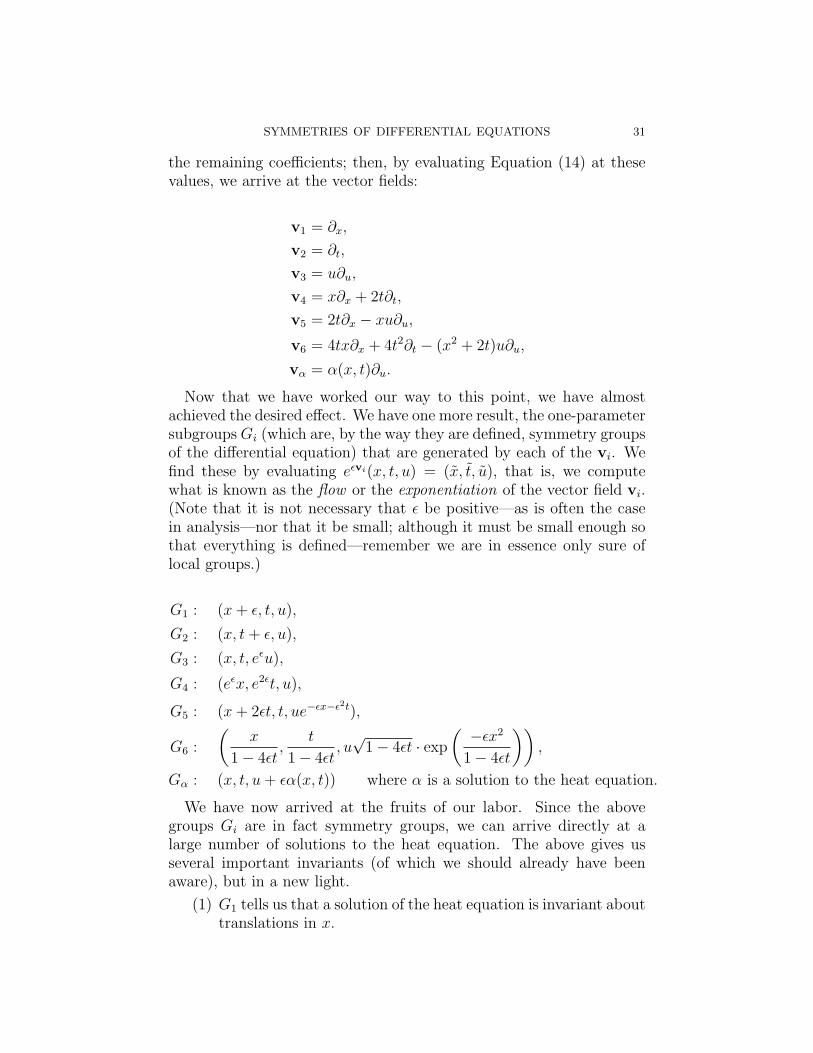
the remaining coefficients; then, by evaluating Equation (14) at thesevalues, we arrive at the vector fields:
v1 = ∂x,
v2 = ∂t,
v3 = u∂u,
v4 = x∂x + 2t∂t,
v5 = 2t∂x − xu∂u,
v6 = 4tx∂x + 4t2∂t − (x2 + 2t)u∂u,
vα = α(x, t)∂u.
Now that we have worked our way to this point, we have almostachieved the desired effect. We have one more result, the one-parametersubgroupsGi (which are, by the way they are defined, symmetry groupsof the differential equation) that are generated by each of the vi. Wefind these by evaluating eεvi(x, t, u) = (x, t, u), that is, we computewhat is known as the flow or the exponentiation of the vector field vi.(Note that it is not necessary that ε be positive—as is often the casein analysis—nor that it be small; although it must be small enough sothat everything is defined—remember we are in essence only sure oflocal groups.)
G1 : (x+ ε, t, u),
G2 : (x, t+ ε, u),
G3 : (x, t, eεu),
G4 : (eεx, e2εt, u),
G5 : (x+ 2εt, t, ue−εx−ε2t),
G6 :
(x
1− 4εt,
t
1− 4εt, u√
1− 4εt · exp
(−εx2
1− 4εt
)),
Gα : (x, t, u+ εα(x, t)) where α is a solution to the heat equation.
We have now arrived at the fruits of our labor. Since the abovegroups Gi are in fact symmetry groups, we can arrive directly at alarge number of solutions to the heat equation. The above gives usseveral important invariants (of which we should already have beenaware), but in a new light.
(1) G1 tells us that a solution of the heat equation is invariant abouttranslations in x.

32 JACOB HARRY BURKMAN
(2) G2 gives the analogous result for translations in t.(3) G3 tells us that at least any positive multiple of a solution is
also a solution.(4) G4 gives us a well known scaling symmetry.(5) G5 is something that may not be entirely recognizable. (It is a
Galilean boost to a moving coordinate frame).17
(6) G6 is unnatural (being a full-fledged local group of transforma-tions), but has many nice consequences including the possiblyunintuitive “Fundamental Source Solution.”
(7) Gα is the superposition principle.
One thing to note is that every homogeneous linear differential equa-tion will have the symmetries of scaling (3) and superposition (7); sothese clearly are not unique to the heat equation.
In Bleecker & Csordas Exercise 1 p. 135, we are asked to show thatgiven a solution u(x, t) of the heat equation, various transformations ofu(x, t) provide new solutions. While these solutions can be verified in astraight forward manner using differentiation, they can also be shownby making use of the above symmetry groups.
We now derive the solution
u(x, t) =1√4πt
e−x2
4t , t > 0, −∞ < x <∞
of Equation (12) using the above results (see [Olv93] p. 120).
Proof. From G6, we see that if an arbitrary function u = f(x, t) is asolution of the heat equation, so is
v = g(x, t) =1√
1 + 4εte−εx2
1+4εtf
(x
1 + 4εt,
t
1 + 4εt
)for any ε in a proper neighborhood of the origin. Now clearlyu = f(x, t) = c is a solution of the heat equation for any constant c.Hence we have that
v1 =c√
1 + 4εte−εx2
1+4εt
17This symmetry group gives the standard product solutions if we let ε be com-plex, see [BC96] exercise 7 and 8 p. 137

SYMMETRIES OF DIFFERENTIAL EQUATIONS 33
is a solution of the heat equation. But this holds for any value of c, soin particular, it holds if we set c =
√επ, giving the solution
v2 =
√ε
π(1 + 4εt)e−εx2
1+4εt .
We can see that v2 is algebraically equivalent to
v3 =1√
4π(t+ 1
4ε
)e −x2
4(t+ 14ε)
by multiplying surreptitiously by14ε14ε
. We now apply G2 and translate
v3 “right” 14ε
in t. This gives us the Fundamental Source Solution tothe heat equation.
In a previous example (c.f. Example 4), we had derived the functionφx using Lie Derivatives. The method of Lie Derivatives has certainadvantages, but it has one major disadvantage for finding the prolonga-tion formulas—it is necessary to have foreknowledge of the differentialform that remains invariant. There is a method that does not ac-tually require this foreknowledge; for the next example, we will usethis method in computing the prolongation formulas (in the interest ofspace and not including too many excess calculations, only a completederivation for x is included). The example will be the wave equation,but before we get into that we introduce the notion of a total derivative.
Definition 24. Let P (x, u(n)) be a smooth function of x, u and thederivatives of u up to order n, defined on an open subset M (n) ⊂X ×U (n). The total derivative of P with respect to xi is the uniquesmooth function (DiP )(x, u(n+1)) defined on M (n+1) and depending onderivatives of u up to order n+1, with the property that if u = f(x) is
any smooth function, (DiP )(x, pr(n+1) f(x)) = ∂∂xi
(P (x, pr(n) f(x))
).
There are several comments that should be made in regards to thisdefinition. First remember that by X we are referring to the entirespace of independent variables. Second, if φ is a function on an n-jet,then Diφ is actually a function on an (n + 1)-jet. Finally, the totalderivative is a generalization of the chain rule; for instance, supposewe have a function ξ(x, y, t, u) defined on the 0-jet (which is locallydiffeomorphic to the space R3 × R), then
D1ξ = Dxξ =∂ξ
∂x+ ux
∂ξ
∂u.
34 JACOB HARRY BURKMAN
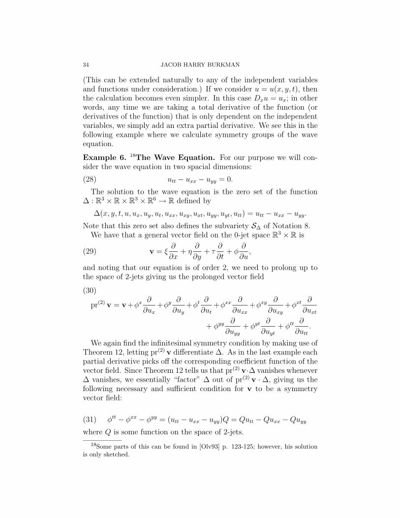
(This can be extended naturally to any of the independent variablesand functions under consideration.) If we consider u = u(x, y, t), thenthe calculation becomes even simpler. In this case Dxu = ux; in otherwords, any time we are taking a total derivative of the function (orderivatives of the function) that is only dependent on the independentvariables, we simply add an extra partial derivative. We see this in thefollowing example where we calculate symmetry groups of the waveequation.
Example 6. 18The Wave Equation. For our purpose we will con-sider the wave equation in two spacial dimensions:
(28) utt − uxx − uyy = 0.
The solution to the wave equation is the zero set of the function∆ : R3 × R× R3 × R6 → R defined by
∆(x, y, t, u, ux, uy, ut, uxx, uxy, uxt, uyy, uyt, utt) = utt − uxx − uyy.
Note that this zero set also defines the subvariety S∆ of Notation 8.We have that a general vector field on the 0-jet space R3 × R is
(29) v = ξ∂
∂x+ η
∂
∂y+ τ
∂
∂t+ φ
∂
∂u,
and noting that our equation is of order 2, we need to prolong up tothe space of 2-jets giving us the prolonged vector field
(30)
pr(2) v = v+φx ∂
∂ux
+φy ∂
∂uy
+φt ∂
∂ut
+φxx ∂
∂uxx
+φxy ∂
∂uxy
+φxt ∂
∂uxt
+ φyy ∂
∂uyy
+ φyt ∂
∂uyt
+ φtt ∂
∂utt
.
We again find the infinitesimal symmetry condition by making use ofTheorem 12, letting pr(2) v differentiate ∆. As in the last example eachpartial derivative picks off the corresponding coefficient function of thevector field. Since Theorem 12 tells us that pr(2) v·∆ vanishes whenever∆ vanishes, we essentially “factor” ∆ out of pr(2) v · ∆, giving us thefollowing necessary and sufficient condition for v to be a symmetryvector field:
(31) φtt − φxx − φyy = (utt − uxx − uyy)Q = Qutt −Quxx −Quyy
where Q is some function on the space of 2-jets.
18Some parts of this can be found in [Olv93] p. 123-125; however, his solutionis only sketched.

SYMMETRIES OF DIFFERENTIAL EQUATIONS 35
We will now, as promised, calculate the prolongations. But first weneed a definition.
Definition 25. The characteristic of v (c.f. Equation (29)) in thecase where X × U ∼= R3 × R (suitable changes can easily be madedepending on the number of independent variables) is the functionφ− ξux − ηuy − τut.
In the prolongation formula (see [Olv93] p. 110), we are told that,in the wave equation,
φx = Dx(φ− ξux − ηuy − τut) + ξuxx + ηuxy + τuxt.
Remember that φx is a function on the 1-jets, and thus should only bedependent up to first order derivatives; however, also remember thatDx pushes the function up the the next jet. We perform the abovecalculation, remembering the above comments on how Dx works andrealizing that it obeys linearity and the product rule.
φx = Dx(φ− ξux − ηuy − τut) + ξuxx + ηuxy + τuxt
= Dxφ− (ξDxux + uxDxξ)− (ηDxuy + uyDxη)
− (τDxut + utDxτ) + ξuxx + ηuxy + τuxt
= Dxφ− ξuxx − uxDxξ − ηuxy − uyDxη − τuxt − utDxτ
+ ξuxx + ηuxy + τuxt
= Dxφ− uxDxξ − uyDxη − utDxτ
=
(∂φ
∂x+ ux
∂φ
∂u
)− ux
(∂ξ
∂x+ ux
∂ξ
∂u
)− uy
(∂η
∂x+ ux
∂η
∂u
)− ut
(∂τ
∂x+ ux
∂τ
∂u
)= φx + φuux − ξxux − ξuu2
x − ηxuy − ηuuxuy − τxut − τuuxut
= φx + (φu − ξx)ux − ηxuy − τxut − ξuu2x − ηuuxuy − τuuxut.
Notice that indeed we do get that φx is really only a function on the1-jet (despite it looking like it may not be originally). We will wishto consider all of these prolongation formulas as “polynomials” withindeterminants being the partial derivatives of u.
The remaining 1st prolongation formulas are
φy = Dy(φ− ξux − ηuy − τut) + ξuxy + ηuyy + τuyt
= φy − ξyux + (φu − ηy)uy − τyut − ξuuxuy − ηuu2y − τuuyut

36 JACOB HARRY BURKMAN
and
φt = Dt(φ− ξux − ηuy − τut) + ξuxt + ηuyt + τutt
= φt − ξtux − ηtuy + (φu − τt)ut − ξuuxut − ηuutuy − τuu2t .
We now calculate the second prolongation, φxx, recalling the recur-sive nature of prolongation.
φxx = Dx(φx − ξuxx − ηuxy − τuxt) + ξuxxx + ηuxxy + τuxxt
(32)
= Dxφx − (ξDxuxx + uxxDxξ)− (ηDxuxy + uxyDxη)
− (τDxuxt + uxtDxτ) + ξuxxx + ηuxxy + τuxxt
= Dxφx − ξuxxx − uxxDxξ − ηuxxy − uxyDxη − τuxxt − uxtDxτ
+ ξuxxx + ηuxxy + τuxxt
= Dxφx − uxxDxξ − uxyDxη − uxtDxτ
=
(∂φx
∂x+ ux
∂φx
∂u
)− uxx
(∂ξ
∂x+ ux
∂ξ
∂u
)− uxy
(∂η
∂x+ ux
∂η
∂u
)− uxt
(∂τ
∂x+ ux
∂τ
∂u
)= φx
x + φxuux − ξxuxx − ξuuxuxx − ηxuxy − ηuuxuxy − τxuxt − τuuxuxt
=(φxx + φuuxx − ξxuxx + φxuux − ξxxux − ηxuxy − ηxxuy − τxuxt
− τxxut − 2ξuuxuxx − ξxuu2x − ηuuxuxy − ηuuyuxx − ηuuyuxx
− ηxuuxuy − τuuxuxt − τuutuxx − τxuuxut
)+
(φxuux + φuuu
2x
− ξxuu2x − ηxuuxuy − τxuuxut − ξuuu
3x − ηuuu
2xuy − τuuu
2xut
)− ξxuxx − ξuuxuxx − ηxuxy − τxuxt − τuuxuxt
= φxx + (2φxu − ξxx)ux − ηxxuy − τxxut + (φuu − 2ξxu)u2x − 2ηxuuxuy
− 2τxuuxut + (φu − 2ξx)uxx − 2τxuxt − 2ηxuxy − ξuuu3x − ηuuu
2xuy
− τuuu2xut − 3ξuuxuxx − ηuuyuxx − τutuxx − 2ηuuxuxy − 2τuuxuxt.
Since the calculations for φyy and φtt are essentially identical to thatfor φxx above, we will not include these values here. Also, there is apattern in the calculation of these prolongations, so once one discoversthis pattern, actually computing them is unnecessary. However, we areinterested in the left hand side of Equation (31), so we include thathere (even though it is very ungainly).

SYMMETRIES OF DIFFERENTIAL EQUATIONS 37
φtt − φxx − φyy = (φtt − φxx − φyy) + (−ξtt − 2φxu + ξxx + ξyy)ux
(33a)
+(−ηtt + ηxx − 2φyu + ηyy)uy + (2φtu − τtt + τxx + τyy)ut(33b)
−(φuu − 2ξxu)u2x − (φuu − 2ηyu)u
2y + (φuu − 2τtu)u
2t(33c)
+(2ηxu + 2ξyu)uxuy + (τxu − 2ξtu)uxut + (2τyu − 2ηtu)uyut(33d)
−(φu − 2ξx)uxx − (φu − 2ηy)uyy + (φu − 2τt)utt(33e)
+(2τx − 2ξt)uxt + (2ηx + 2ξy)uxy + (2τy − 2ηt)uyt(33f)
+ξuuu3x + ηuuu
3y − τuuu
3t(33g)
+ηuuu2xuy + τuuu
2xut + ξuuuxu
2y + τuuutu
2y − ηuuuyu
2t − ξuuuxu
2t(33h)
+3ξuuxuxx + 3ηuuyuyy − 3τuututt + ηuuyuxx + τuutuxx(33i)
+ξuuxuyy + τuutuyy − ηuuyutt − ξuuxutt + 2ηuuxuxy + 2τuuxuxt(33j)
+2ξuuyuxy + 2τuuyuyt − 2ηuutuyt − 2ξuutuxt.(33k)
Recalling that φtt− φxx− φyy = (utt− uxx− uyy)Q = Qutt−Quxx−Quyy, we eventually see that almost all of the terms in Equation (33)are actually 0. When we identified the symmetry Lie algebra for theheat equation in the last example, we dealt with it as a whole. In thiscase, we will do what is more commonly the practice in dealing withthis type of problem, namely to “tackle the solution of the symme-try equations in stages, first extracting information from higher orderderivatives appearing in them, and then using this information to sim-plify the prolongation formulas.”19 This is often the most efficient wayto analyze such problems (for the wave equation, as far as differen-tial equations go, is fairly straightforward), and we already have anequation that is very long, and attempting to write down all the corre-sponding partial differential equations we would need to solve would beeven longer. In this case, we first consider the coefficients of the secondorder derivatives, uxy, uxt, uyt, uxx, uyy, utt (these are in lines (33f), (33j)and (33k) of Equation (33)). Since everything on the right hand sideof Equation (31) needs to contains at least uxx, uyy, utt, the coefficientfunctions of uxy, uxt, uyt must be 0. With these, we see
19See [Olv93] p. 121.

38 JACOB HARRY BURKMAN
uxt : (2τx − 2ξt) + 2τuux − 2ξuut = 0,
uxy : (2ηx + 2ξy) + 2ηuux + 2ξuuy = 0,
uyt : (2τy − 2ηt) + 2τuuy − 2ηuut = 0.
If we consider the above to be functions on the 1-jets, we noticethat they are linear “polynomials.” Since they are equal to 0, we cansee from basic polynomial facts each of the coefficients are 0 (the onlyway to have the 0 polynomial is for all of its coefficients to be 0). Inparticular, for the constant terms, we have
(34) τx − ξt = 0, ηx + ξy = 0, τy − ηt = 0.
If we look at the other terms, we see that τu = 0, ξu = 0, ηu = 0.This implies that none of these are a function of u, hence we havethat ξ = ξ(x, y, t), η = η(x, y, t), τ = τ(x, y, t). Note that this resultmeans that all the terms in lines (33g), (33h), (33i), (33j), and (33k) ofEquation (33) are 0. This is a major simplification of Equation (33),and that is our (and Lie’s) goal in using this method to understanddifferential equations.
We can also see that the coefficients of uxx, uyy, utt imply that
Q = φu − 2ξx = φu − 2ηy = φu − 2τt.
So clearly we have the result that
(35) τt = ξx = ηy.
The reader may recognize that Equations (34) and (35) are the equa-tions for an infinitesimal conformal transformation on R3 with Lorentzmetric dt2 − dx2 − dy2 (see [Olv93] p. 123).
Using substitutions from Equations (34) and (35) and taking deriva-tives, we can see that (the first is from Olver, we do two other calcula-tions)
ξxxx = ηxxy = −ξxyy = −τyyt = −ηytt = −ξxtt = −τxxt = −ξxxx,
ηyyy = ξxyy = −ηxxy = −τxxt = −ξxtt = −ηytt = −τyyt = −ηyyy,
ξyyy = −ηxyy = −τxyt = −ξtty = ηttx = τytx = ηyyx(= −ξyyy).
The last equality in the third line is included only to continue thepattern, for by saying that −ηxyy = ηyyx we already have that theentire string, including ξyyy, is equal to 0.
Doing similar calculations, i.e. showing that all the possible thirdorder derivatives of ξ, τ, η are actually equal to their opposite, we can

SYMMETRIES OF DIFFERENTIAL EQUATIONS 39
see that they are all 0. Hence ξ, τ, η are at most quadratic in each ofx, y, t. Hence, by using the relations in Equations (34) and (35), wecan actually find that
ξ = c1 + c4x− c5y + c6t+ c8(x2 − y2 + t2) + 2c9xy + 2c10xt,
η = c2 + c5x+ c4y + c7t+ 2c8xy + c9(−x2 + y2 + t2) + 2c10yt,
τ = c3 + c6x+ c7y + c4t+ 2c8xt+ 2c9yt+ c10(x2 + y2 + t2),
where c1, . . . , c10 are arbitrary constants.Now since all of the indeterminants u2
x, u2y, u
2t do not appear in the
right hand side of Equation (31), we must have that the coefficientsof u2
x, u2y, u
2t in Equation (33) must be 0 (that is all the coefficients in
(33c) are 0); since we have already shown that none of ξ, η, τ dependon u, it follows that φuu = 0. Hence φ is at most linear in u, so we canwrite
φ(x, y, t, u) = β(x, y, t)u+ α(x, y, t).
We then finally examine the constant terms and the first order deriva-tives of Equation (33) (they’re in line (33a)), finding the following re-lations:
2βx = ξxx + ξyy − ξtt,2βy = ηxx + ηyy − ηtt,
2βt = τtt − τxx − τyy,
αtt − αxx − αyy = 0.
Hence we can see that α is an (arbitrary) solution to the wave equa-tion, and by making use of our previous definitions of ξ, η, τ , we cansee that
β = c11 − c8x− c9y − c10t.
We find the infinitesimal symmetries in the same way as we did inthe example of the heat equation—by successively setting the constantsequal to 1 and the rest equal to 0. The first 10 generate the conformalalgebra for R3 with the given Lorentz metric.
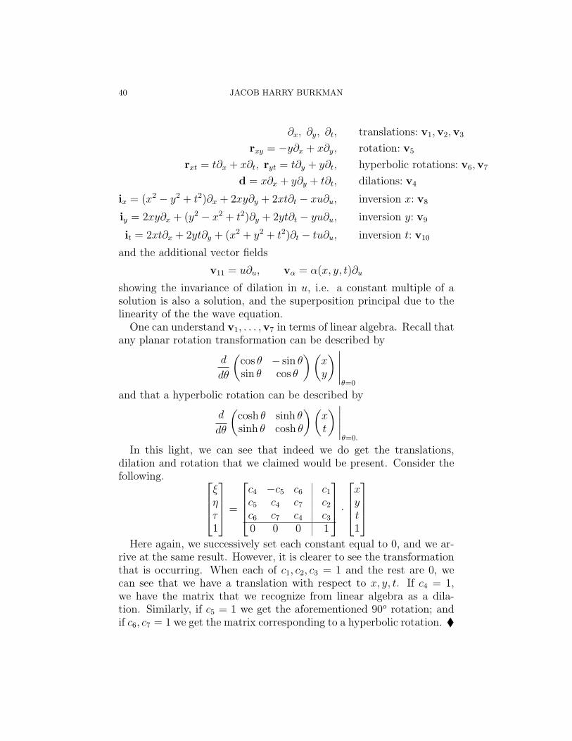
40 JACOB HARRY BURKMAN
∂x, ∂y, ∂t, translations: v1,v2,v3
rxy = −y∂x + x∂y, rotation: v5
rxt = t∂x + x∂t, ryt = t∂y + y∂t, hyperbolic rotations: v6,v7
d = x∂x + y∂y + t∂t, dilations: v4
ix = (x2 − y2 + t2)∂x + 2xy∂y + 2xt∂t − xu∂u, inversion x: v8
iy = 2xy∂x + (y2 − x2 + t2)∂y + 2yt∂t − yu∂u, inversion y: v9
it = 2xt∂x + 2yt∂y + (x2 + y2 + t2)∂t − tu∂u, inversion t: v10
and the additional vector fields
v11 = u∂u, vα = α(x, y, t)∂u
showing the invariance of dilation in u, i.e. a constant multiple of asolution is also a solution, and the superposition principal due to thelinearity of the the wave equation.
One can understand v1, . . . ,v7 in terms of linear algebra. Recall thatany planar rotation transformation can be described by
d
dθ
(cos θ − sin θsin θ cos θ
) (xy
) ∣∣∣∣∣θ=0
and that a hyperbolic rotation can be described by
d
dθ
(cosh θ sinh θsinh θ cosh θ
) (xt
) ∣∣∣∣∣θ=0.
In this light, we can see that indeed we do get the translations,dilation and rotation that we claimed would be present. Consider thefollowing.
ξητ1
=
c4 −c5 c6 c1c5 c4 c7 c2c6 c7 c4 c30 0 0 1
·xyt1
Here again, we successively set each constant equal to 0, and we ar-
rive at the same result. However, it is clearer to see the transformationthat is occurring. When each of c1, c2, c3 = 1 and the rest are 0, wecan see that we have a translation with respect to x, y, t. If c4 = 1,we have the matrix that we recognize from linear algebra as a dila-tion. Similarly, if c5 = 1 we get the aforementioned 90o rotation; andif c6, c7 = 1 we get the matrix corresponding to a hyperbolic rotation.
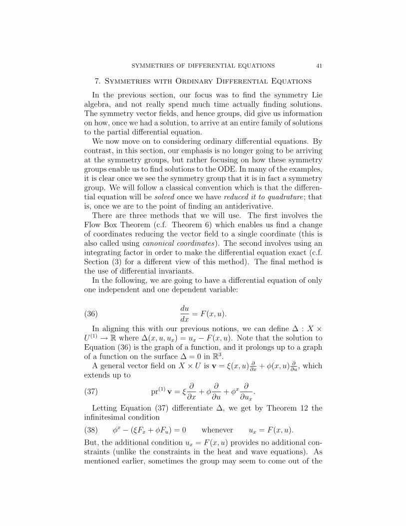
SYMMETRIES OF DIFFERENTIAL EQUATIONS 41
7. Symmetries with Ordinary Differential Equations
In the previous section, our focus was to find the symmetry Liealgebra, and not really spend much time actually finding solutions.The symmetry vector fields, and hence groups, did give us informationon how, once we had a solution, to arrive at an entire family of solutionsto the partial differential equation.
We now move on to considering ordinary differential equations. Bycontrast, in this section, our emphasis is no longer going to be arrivingat the symmetry groups, but rather focusing on how these symmetrygroups enable us to find solutions to the ODE. In many of the examples,it is clear once we see the symmetry group that it is in fact a symmetrygroup. We will follow a classical convention which is that the differen-tial equation will be solved once we have reduced it to quadrature; thatis, once we are to the point of finding an antiderivative.
There are three methods that we will use. The first involves theFlow Box Theorem (c.f. Theorem 6) which enables us find a changeof coordinates reducing the vector field to a single coordinate (this isalso called using canonical coordinates). The second involves using anintegrating factor in order to make the differential equation exact (c.f.Section (3) for a different view of this method). The final method isthe use of differential invariants.
In the following, we are going to have a differential equation of onlyone independent and one dependent variable:
(36)du
dx= F (x, u).
In aligning this with our previous notions, we can define ∆ : X ×U (1) → R where ∆(x, u, ux) = ux − F (x, u). Note that the solution toEquation (36) is the graph of a function, and it prolongs up to a graphof a function on the surface ∆ = 0 in R3.
A general vector field on X × U is v = ξ(x, u) ∂∂x
+ φ(x, u) ∂∂u
, whichextends up to
(37) pr(1) v = ξ∂
∂x+ φ
∂
∂u+ φx ∂
∂ux
.
Letting Equation (37) differentiate ∆, we get by Theorem 12 theinfinitesimal condition
(38) φx − (ξFx + φFu) = 0 whenever ux = F (x, u).
But, the additional condition ux = F (x, u) provides no additional con-straints (unlike the constraints in the heat and wave equations). Asmentioned earlier, sometimes the group may seem to come out of the

42 JACOB HARRY BURKMAN
blue. This is because “solving Equation (38) is often much more dif-ficult that solving Equation (36). However, led on by inspired-guesswork, or geometric intuition, we may be able to ascertain a particularsolution to Equation (38) which will allow us to integrate Equation(36). Herein lies the art of Lie’s method.”20 As we have seen earlier,Lie was someone who would often make some leaps; here we have todo the same.
We now specifically consider the result using the Flow Box Theorem(c.f. Theorem 6). According to this theorem, we can find a change ofcoordinates (in this case the independent variable y = η(x, u) and thedependent variable w = ζ(x, u)) so that the vector field v also changescoordinates into v∗ = ∂
∂w. Since the prolongations involve derivatives
(in this case total derivatives) and the coefficient functions of ∂∂y
and ∂∂w
in v∗ are 0 and 1 respectively, we see that v∗ actually prolongs to itself,i.e. pr(1) v∗ = ∂
∂w. We can further re-express Equation (36) in terms
of the new variables ∆∗ = wy −H(y, w), and letting the prolongationdifferentiate this function, we find the infinitesimal condition
pr(1) v∗ ·∆∗ = −∂H∂w
(y, w) = 0 whenever wy = H(y, w).
This, of course, implies that H does not depend on w; thus we canreduce the differential equation to
dw
dy= H(y) =⇒ w =
∫H(y) dy.
We now look at this in an example.
Example 7. 21 Recall from Section (3) (where we do an alternativetreatment) that a homogeneous equation is a differential equation forwhich F is dependent only on the ration u
x, i.e.
du
dx= F
(ux
).
By inspection, we can see that the 1-parameter group of scalingtransformations Gλ : (x, u) 7→ (λx, λu) (where λ > 0) is a symmetrygroup (let G act on the differential equation, which will replace x withλx and u with λu, and see that the λ′s cancel leaving the equation un-changed). Let λ0 denote the parameter corresponding the the identity
20See [Olv93] p. 131.21See [Olv93] p. 133.
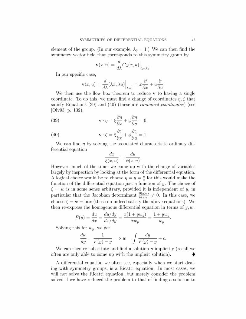
SYMMETRIES OF DIFFERENTIAL EQUATIONS 43
element of the group. (In our example, λ0 = 1.) We can then find thesymmetry vector field that corresponds to this symmetry group by
v(x, u) =d
dλGλ(x, u)
∣∣∣λ=λ0
.
In our specific case,
v(x, u) =d
dλ(λx, λu)
∣∣∣λ=1
= x∂
∂x+ u
∂
∂u.
We then use the flow box theorem to reduce v to having a singlecoordinate. To do this, we must find a change of coordinates η, ζ thatsatisfy Equations (39) and (40) (these are canonical coordinates) (see[Olv93] p. 132).
(39) v · η = ξ∂η
∂x+ φ
∂η
∂u= 0,
(40) v · ζ = ξ∂ζ
∂x+ φ
∂ζ
∂u= 1.
We can find η by solving the associated characteristic ordinary dif-ferential equation
dx
ξ(x, u)=
du
φ(x, u).
However, much of the time, we come up with the change of variableslargely by inspection by looking at the form of the differential equation.A logical choice would be to choose η = y = u
xfor this would make the
function of the differential equation just a function of y. The choice ofζ = w is in some sense arbitrary, provided it is independent of y, in
particular that the Jacobian determinant ∂(y,w)∂(x,u)
6= 0. In this case, we
choose ζ = w = ln x (these do indeed satisfy the above equations). Wethen re-express the homogenous differential equation in terms of y, w.
F (y) =du
dx=du/dy
dx/dy=x(1 + ywy)
xwy
=1 + ywy
wy
.
Solving this for wy, we get
dw
dy=
1
F (y)− y=⇒ w =
∫dy
F (y)− y+ c.
We can then re-substitute and find a solution u implicitly (recall weoften are only able to come up with the implicit solution).
A differential equation we often see, especially when we start deal-ing with symmetry groups, is a Ricatti equation. In most cases, wewill not solve the Ricatti equation, but merely consider the problemsolved if we have reduced the problem to that of finding a solution to

44 JACOB HARRY BURKMAN
a Ricatti equation. Various sources have a variety of equations that onthe surface appear different (but in many senses are very similar) thatthey call Ricatti equations. Bluman has perhaps the simplest form,dudx
= A+Bu+Cu2 (see [BK89] p. 105). Olver relaxes the condition onconstant coefficients and calls the expression zx = −z2 − p(x)z − q(x)a Ricatti equation (see [Olv93] p. 139). We then would consider thata Ricatti equation is one with du
dxbeing quadratic in u. The following
two examples look at solving specific Ricatti equations using canonicalcoordinates.
We earlier concluded symmetry groups must act on solutions by send-ing them to solutions. We will adopt Hydon’s notation (see [Hyd00]p. 8), which is slightly different than Olver’s, for parts of these nextexamples. For instance, we will denote by (x, u) the image of (x, u) un-der the symmetry map. The reader can clearly see that the results arethe same as our earlier approaches. We have previously talked aboutsymmetry conditions of Equation (36) and other differential equations,so here we will skip some of the preliminaries; however, note that thepreviously mentioned methods get us to the equivalent condition (see[Hyd00] p. 8)
(41) F (x, u) =ux + F (x, u)uu
xx + F (x, u)xu
.
Example 8. 22 Solve the Ricatti equation
(42)du
dx= xu2 − 2u
x− 1
x3, (x 6= 0).
Equation (42) has a scaling symmetry
(43) (x, u) = (eεx, e−2εu).
This is easy to see by either using Equation (41), or by simply substi-tuting Equation (43) into Equation (42) and seeing that it is unchangedafter simplification. Noting our previously mentioned methods for de-termining the vector field corresponding to the symmetry (find thevalue of the parameter that is the identity, and then differentiate thiswith respect to the parameter, and then set the parameter equal tothe identity), we find that the symmetry vector field generated by the1-parameter group in Equation (43) is
v = x∂
∂x− 2u
∂
∂u.
22See [Hyd00]. This is a running example in Chapter 2.

SYMMETRIES OF DIFFERENTIAL EQUATIONS 45
As an aside, we can then find what Hydon calls the reduced charac-teristic (see [Hyd00] p. 21),
(44) Q = (φ− uxξ)|(ux=F (x,u)) = φ− Fξ.In the case of Equation (42), we can see that it has reduced character-istic
Q =1
x2− x2u2.
The values of umaking Q = 0 are solutions to Equation (42). We canclearly see that this occurs when u = ±x−2. However, these are not theonly solutions to Equation (42). We will now compute the complete setof solutions for Equation (42). From the above, we already have the twosolutions u = ±x−2. Furthermore, we can get canonical coordinates
(η, ζ) = (x2u, ln |x|)for Equation (42) (c.f. Equations (39) and (40)).
We can then use these to change the coordinates, in line with theFlow Box Theorem, of Equation (42) to the simpler form
dζ
dη=
1
η2 − 1=⇒ ζ =
∫1
η2 − 1dη.
Evaluating this is straightforward, and after re-substituting back tox and u, we arrive at the general solution
u =c+ x2
x2(c− x2).
(In this solution, we see that the solutions of u = ±x−2 are present;u = x−2 is the limit as c → ∞, and u = −x−2 corresponds to thesolution when c = 0.
Hydon also includes another example of a Ricatti equation that wesolve in the next example.
Example 9. 23 Solve the Ricatti Equation
(45)du
dx=u+ 1
x+u2
x3, (x 6= 0).
We claim that one of the symmetries of Equation (45) is
(46) (x, u) =
(x
1− εx,
u
1− εx
).
23See [Hyd00] p. 10-11, 28.

46 JACOB HARRY BURKMAN
This is directly proven by substituting Equation (46) and Equation(45) into Equation (41), and is purely computation, so we do not in-clude it here. (Of course, how it was determined that this was in facta symmetry is a little more mysterious.) One thing of interest to noteis that this symmetry Equation (45) is indeed local—it is not definedfor ε > 1
|x| . This is similar to the case of the inversions that we have
encountered previously (like in the wave equation example).The tangent vector field corresponding to Equation (46) is
v = x2 ∂
∂x+ xu
∂
∂u.
Once we have established the vector field, we can find the canonicalcoordinates
(47) (η, ζ) =
(u
x,−1
x
), (x 6= 0)
for Equation (45) (c.f. Equations (39) and (40)).Using this, we can again change coordinates, reducing Equation (45)
to the ODEdζ
dη=
1
1 + η2.
This now has an obvious solution (we would want our Calculus 1students to recognize it—although many do not)
ζ = tan−1 η + c,
or in terms of x, u:
u = −x tan
(1
x+ c
).
In Section (3) we looked at an example of an exact equation. Wenow do a slightly more general interpretation of this. We first considera total differential equation, that is, an equation of the form
(48) P (x, u)dx+Q(x, u)du = 0.
Equation (48) is exact if there is some function g(x, u) so thatdg = P (x, u)dx + Q(x, u)du. The condition ∂P
∂u= ∂Q
∂xis a necessary
and sufficient condition for the equation P dx +Qdu being exact (see[Olv93] p. 135).
We now consider the case of using an integrating factor.
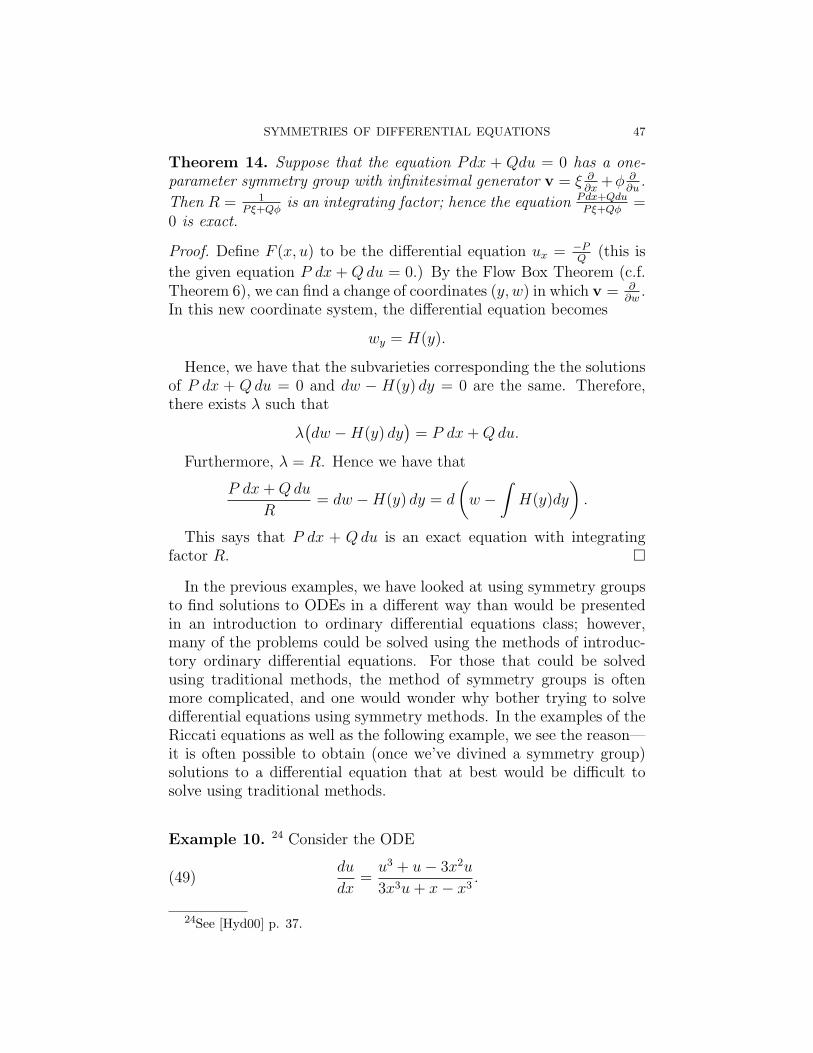
SYMMETRIES OF DIFFERENTIAL EQUATIONS 47
Theorem 14. Suppose that the equation Pdx + Qdu = 0 has a one-parameter symmetry group with infinitesimal generator v = ξ ∂
∂x+φ ∂
∂u.
Then R = 1Pξ+Qφ
is an integrating factor; hence the equation Pdx+QduPξ+Qφ
=0 is exact.
Proof. Define F (x, u) to be the differential equation ux = −PQ
(this is
the given equation P dx +Qdu = 0.) By the Flow Box Theorem (c.f.Theorem 6), we can find a change of coordinates (y, w) in which v = ∂
∂w.
In this new coordinate system, the differential equation becomes
wy = H(y).
Hence, we have that the subvarieties corresponding the the solutionsof P dx + Qdu = 0 and dw − H(y) dy = 0 are the same. Therefore,there exists λ such that
λ(dw −H(y) dy
)= P dx+Qdu.
Furthermore, λ = R. Hence we have that
P dx+Qdu
R= dw −H(y) dy = d
(w −
∫H(y)dy
).
This says that P dx + Qdu is an exact equation with integratingfactor R.
In the previous examples, we have looked at using symmetry groupsto find solutions to ODEs in a different way than would be presentedin an introduction to ordinary differential equations class; however,many of the problems could be solved using the methods of introduc-tory ordinary differential equations. For those that could be solvedusing traditional methods, the method of symmetry groups is oftenmore complicated, and one would wonder why bother trying to solvedifferential equations using symmetry methods. In the examples of theRiccati equations as well as the following example, we see the reason—it is often possible to obtain (once we’ve divined a symmetry group)solutions to a differential equation that at best would be difficult tosolve using traditional methods.
Example 10. 24 Consider the ODE
(49)du
dx=u3 + u− 3x2u
3x3u+ x− x3.
24See [Hyd00] p. 37.

48 JACOB HARRY BURKMAN
The reader familiar with ODE’s can see that this is not reasonablysolvable by any traditional method, such as we have mentioned aboveand in Section (3).
However, note that Equation (49) has an infinitesimal symmetryvector field
v = (u3 + u− 3x2u)∂
∂x+ (x3 − x− 3xu2)
∂
∂u.
We then find that the characteristic equation is
(50)du
dx=x3 − x− 3xu2
u3 + u− 3x2y.
This does not appear to be any more easily solvable than Equation(49). However, we can use an integrating factor (see Theorem 14),noting that ∫
du− Fdxφ− Fξ
= c.
Applying this to Equation (50), we get after doing some calculations∫(x3 − x− 3xu2)du+ (u3 + u− 3x2u)dx
(u2 + x2)(u2 + (x+ 1)2)(u2 + (x− 1)2)= c,
which, finally can be evaluated relatively easily, using partial fractions,to yield the result
1
2tan−1
(u
x+ 1
)+
1
2tan−1
(u
x− 1
)− tan−1
(ux
)= c.
We can use trigonometric identities to reduce the above to the sim-pler form
(u2 + x2)2 + u2 − x2
xu= k
where k is a constant. (We would have been extremely hard pressed tocome up with this by traditional methods.)
As we have seen in these examples, using symmetry groups to solveequations really does have advantages—one can solve certain equationsthat would have been very difficult or impossible with traditional meth-ods.
Another important method for integrating differential equations isto make use of the concept of a differential invariant which we definebelow, but to understand what is going on with these differential in-variants, let us first look at the invariants of group actions.

SYMMETRIES OF DIFFERENTIAL EQUATIONS 49
As an example of this, consider the actions of the group SO(2) onR2. Since SO(2) is a group of matrices that induces rotations on theplane, we can see that the orbit of an element (x, u) ∈ R2 will be acircle about the origin with radius r(x, u) =
√x2 + u2. Notice that on
each orbit the function r(x, u) is constant. That makes r an invariantof this group action. Furthermore, r separates the orbits, that is, if(x, u) and (x, u) are such that they are not on the same orbit, thenr(x, u) 6= r(x, u).
Definition 26. Let G be a local group of transformations acting onM ⊂ X × U . An nth order differential invariant of G is a smoothfunction η : M (n) → R, depending on x, u and the derivatives of u upto order n, such that η is an invariant of the prolonged group actionpr(n) G, that is
η(pr(n) g · (x, u(n))) = η(x, u(n)), (x, u(n)) ∈M (n)
(or that η pr(n) g = η) for all g ∈ G for which pr(n) g · (x, u(n)) isdefined.
Dimensions worked nicely in the case of SO(2) acting on R2 to thepoint that we didn’t need to prolong the group action. However, this isnot always the case. We may need to prolong the group action to thejet spaces in order to get a dimension greater than that of the group,for the orbits foliate the jet space by defining submanifolds that havethe same dimension as the group. This enables us to find independentfunctions that are constant on orbits and jointly obtain different valuesfor different orbits.
There are several theorems which enable us to determine differentialinvariants. We note these here (see [Olv93] p. 140-142).
Theorem 15. Let G be a group of transformations acting on M ⊂X × U ∼= R2. Suppose that y = η(x, u(n)) and w = ζ(x, u(n)) are nth
order differential invariants of G. Then the derivative
dw
dy=dw/dx
dy/dx=Dxζ
Dxη
(where Dx is the total derivative) is an (n + 1)st order differential in-variant of G.
Definition 27. A set h1, h2, . . . , hn forms a complete set offunctionally independent invariants for a prolongations if theyare invariants for which there does not exist a function f such thatf(h1, h2, . . . , hn) = 0 (that is they are functionally independent), and

50 JACOB HARRY BURKMAN
if g is any other invariant, then there exists a function F , such thatF (g, h1, . . . , hn) = 0.
Theorem 16. Suppose that G is a one-parameter group of transforma-tions acting on M ⊂ X ×U ∼= R2. Let y = η(x, u) and w = ζ(x, u, ux)be a complete set of functionally independent invariants of the firstprolongation pr(1)G. Then the derivatives
y, w,dw
dy, . . . ,
dn−1w
dyn−1
provide a complete set of functionally independent invariants for thenth prolongation pr(n)G for n ≥ 1.
Example 11. As an example of how this theorem works, consider theexample of SO(2) acting on the plane. Then clearly the function y =√x2 + u2 is a zero order differential invariant (that is, it is invariant on
the 0-jet). Furthermore, we can construct a second differential invariant(which will be on the 1-jets) by considering that for SO(2),
pr(1) v = −u ∂∂x
+ x∂
∂u+ (1 + u2
x)∂
∂ux
.
From this, we can see that the characteristic equation is
dx
−u=du
x=
dux
1 + u2x
.
Incorporating the known invariant r via the relation x =√r2 − u2, we
can restate this characteristic equation as a separable equation
du√r2 − u2
=dux
1 + u2x
,
which shows us that
sin−1(ur
)= tan−1 ux + k
where k is a constant. We can use right triangle trigonometry to showthat we have the relation
tan−1 ux − tan−1(ux
)= k.
Then, we take the tangent of each side, and make use of the formulatan(α− β) = tan α−tan β
1+tan α tan β, we see that
(51) w :=xux − ux+ uux
= constant.
This shows us that the left hand side of equation (51) is actually aninvariant of pr(1) SO(2) that is a function on the 1-jet. Furthermore, it

SYMMETRIES OF DIFFERENTIAL EQUATIONS 51
is independent from√x2 + u2 since the former is clearly dependent on
ux whereas the latter is not.Geometric intuition tells us that the curvature, κ, is also invariant
under SO(2). What Theorem 16 tells us is that we should be able toexpress the curvature,
κ =uxx
(1 + u2x)
(3/2)
which is a function on the 2-jets (and hence invariant under the second
prolongation), as a function κ = κ(y, w, dw
dy
). We compute this latter
derivative.
wy =dw
dy=dw/dx
dy/dx=
√x2 − u2
(x+ uux)3
((x2 + u2)uxx − (1 + u2
x)(xux − u)).
Again, it is clear that this is functionally independent from y, w. Onecan readily check that
κ =uxx
(1 + u2x)
(3/2)=
wy
(1 + w2)(3/2)+
w
y(1 + w2)(1/2).
(Equivalently, we could have written wy as a function of y, w, κ.) It is astraightforward calculation to show that κ and wy are in fact invariantsby letting pr(2) v differentiate either of these and seeing that the resultis 0.
This shows us that once we have a compete set of independent in-variants for a particular prolongation (we use dimensions to determinehow many there should be), then any other invariant must be able tobe written as a function of those invariants.
For instance, the most general first order ordinary differential equa-tion admitting SO(2) is
xux − ux+ uux
= H(√x2 + u2)
where H is an arbitrary function (see [BK89] p. 107).
One more theorem completes our list. This theorem deals with reduc-tion of order, and as such, is very similar to Lie’s Theorem 7; however,it includes some of the formality that was absent in that theorem.
Theorem 17. Let G be a local group of transformations acting onM ⊂ X × U . Assume pr(n)G acts in such a way that all orbits ofthe action have the same dimension on an open subset of M (n), andlet η1(x, u(n)), . . . , ηk(x, u(n)) be a complete set of functionally indepen-dent nth order differential invariants. An nth order differential equation
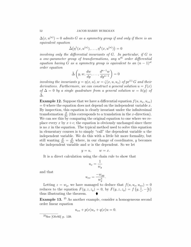
52 JACOB HARRY BURKMAN
∆(x, u(n)) = 0 admits G as a symmetry group if and only if there is anequivalent equation
∆(η1(x, u(n)), . . . , ηk(x, u(n))
)= 0
involving only the differential invariants of G. In particular, if G isa one-parameter group of transformations, any nth order differentialequation having G as a symmetry group is equivalent to an (n − 1)st
order equation
∆
(y, w,
dw
dy, . . . ,
dn−1w
dyn−1
)= 0
involving the invariants y = η(x, u), w = ζ(x, u, ux) of pr(1)G and theirderivatives. Furthermore, we can construct a general solution u = f(x)of ∆ = 0 by a single quadrature from a general solution w = h(y) of∆.
Example 12. Suppose that we have a differential equation f(u, ux, uxx)= 0 where the equation does not depend on the independent variable x.By inspection, this equation is clearly invariant under the infinitesimaltransformation ∂
∂x(this corresponds to a translation in the x-direction).
We can see this by comparing the original equation to one where we re-place every x by x+ ε; the equation is obviously unchanged since thereis no x in the equation. The typical method used to solve this equationin elementary courses is to simply “call” the dependent variable u theindependent variable. We do this with a little bit more formality, butstill wanting ∂
∂x= ∂
∂wwhere, in our change of coordinates, y becomes
the independent variable and w is the dependent. So we let
y = u, w = x.
It is a direct calculation using the chain rule to show that
ux =1
wy
and that
uxx =−wyy
w3y
.
Letting z = wy, we have managed to deduce that f(u, ux, uxx) = 0reduces to the equation F (y, z, zy) = 0, by F (y, z, zy) = f
(y, 1
z,− zy
z3
)thus illustrating the theorem.
Example 13. 25 As another example, consider a homogeneous secondorder linear equation
uxx + p(x)ux + q(x)u = 0.
25See [Olv93] p. 139.

SYMMETRIES OF DIFFERENTIAL EQUATIONS 53
Again, by inspection, we see that this has a symmetry group, namelythe group
Gλ : (x, u) 7→ (x, λu),
since replacing all the u’s by λu leaves the equation unchanged (sinceit is homogeneous linear). This scaling has an infinitesimal generator
v = u∂
∂u.
Noting that the characteristic equation is
dx
0=du
u= d(log u),
we see that x is constant, and that a suitable change of coordinates(in line with Theorem 6) is y = x and w = log u ⇒ u = ew (providedthat u 6= 0, in which case the equation is trivial). With this change ofcoordinates, we can see that
v =∂
∂w.
Furthermore, by differentiation of the change of variable results, wecan see that
ux = ewwy, and uxx = (wyy + w2y)e
w.
Now, we substitute these results back into our equation, arriving atthe equation
ew(wyy + w2y) + p(y)wye
w + q(y)ew = 0
and noting that ew 6= 0 ∀w, we rewrite this as
wyy + w2y + p(y)wy + q(y) = 0
which does not explicitly depend on w, like in the previous example.So, as in that example, we make use of the substitution z = wy arrivingat the new equation
zy + z2 + p(y)z + q(y) = 0
or equivalently, the first order Riccati equation
(52) zy = −z2 − p(y)z − q(y).
We make only a slight foray into equations that admit multi-paramet-er symmetry groups, since much of the analysis is similar to that abovewhere the equation admits a single parameter symmetry group. Inthat case, we are able to reduce the order of the equation by one. Now

54 JACOB HARRY BURKMAN
suppose that ∆(x, u(n)) = 0 admits an r-dimensional (or parameter)symmetry group G. Our intuition tells us that we should be able toreduce the order to an (n− r)th order differential equation. In general,this is true; however, it may not be possible to reconstruct the solutionsto the nth order original equation from these by quadrature alone (re-member that in order for us to consider a differential equation “solved”we must be left only with evaluating an antiderivative). In our case, wewill assume that the rth prolongation pr(r)G has r-dimensional orbitson X×U (r); we make this assumption to avoid some technically compli-cated degenerate cases. This will imply that there are two independentrth order differential invariants
(53) y = η(x, u(r)), w = ζ(x, u(r)).
Furthermore, by noting that r = dimension of orbits ≤ dimension G =r, we see that the orbits will remain r-dimensional for any further pro-longations. Hence by Theorem 16, we can arrive at a complete set ofindependent invariants
y, w,dw
dy,d2w
dy2, . . . ,
dn−rw
dyn−r.
By Theorem 17, since ∆(x, u(n)) = 0 by assumption, we have that thereexists an equivalent ODE, ∆, such that
(54) ∆
(y, w,
dw
dy, . . . ,
dn−rw
dyn−r
)= 0.
So, here we have, in Equation (54), essentially reduced the problemto solving an (n−r)th order equation. However, “the principle problemat this juncture is that it is unclear how we determine the solutionu = f(x) of the original system from the general solution w = h(y) ofthe reduced system (54).”26 We consider this in the following example.
Example 14. Let SL(2) act on R×R by the action of linear fractionaltransformation on the first factor,
(x, u) 7→(αx+ β
γx+ δ, u
).
Note, that since (α βγ δ
)∈ SL(2),∣∣∣∣α β
γ δ
∣∣∣∣ = 1.
26See [Olv93] p. 145.

SYMMETRIES OF DIFFERENTIAL EQUATIONS 55
This determinant condition gives a restriction on the parametersα, β, γ, δ; thus we consider SL(2) to be a 3-parameter group.
This action has the generators corresponding to the transformations
v1 =∂
∂x
(1 β0 1
)translation,
v2 = 2x∂
∂x
(α 00 α−1
)dilation,
v3 = x2 ∂
∂x
(1 0−γ 1
)inversion.
The space X ×U (3) has general coordinates (x, u, ux, uxx, uxxx), so itis five dimensional. Furthermore SL(2) is three dimensional, so it hasorbits that are three dimensional. Hence there are two invariants. (Thenumber of invariants is the codimension of the orbits.) The invarianty = u on the 0-jet is obvious. Much less obvious is the Schwarzianderivative
w = 2u−3x uxxx − 3u−4
x u2xx.
How this is arrived at is a bit of a mystery (it is a rather involved pro-cess that follows from the linear fractional transformation); however, itis computational (and the calculation is not particularly informative)to check that it is invariant under pr(3) vi, i = 1, 2, 3. Since y, w areclearly independent, and there are only two differential invariants, itfollows that these two form a complete set of functionally independentinvariants for the prolongation of pr(3) SL(2).
Hence if ∆(x, u(n)) = 0 is invariant under this action, we must havethat ∆ is equivalent to a (n− 3)rd order equation
(55) ∆
(y, w,
dw
dy, . . . ,
dn−3w
dyn−3
)= 0
involving only the invariants of pr(n) SL(2). Suppose that we havearrived at a solution w = h(y) for Equation (55). Then by using thefact that the Schwarzian derivative is an invariant, we must have that
(56) 2u−3x uxxx − 3u−4
x u2xx = h(u),
which is equivalent to
(57) 2uxuxxx − 3u2xx = u4
xh(u).
In order to find a solution u = f(x) of ∆(x, u(n)) = 0, we must finda solution, u = f(x), of Equation (57). Note that Equation (57) isinvariant under SL(2) since it is equivalent to Equation (56) which canbe written entirely in terms of the invariants. So, we can try to use

56 JACOB HARRY BURKMAN
this knowledge to integrate it. Letting y = u, z = ux, we can rewriteequation (57) as
(58) 2zd2z
dy2−
(dz
dy
)2
= z2h(y)
which is clearly invariant under the scaling (y, z) 7→ (y, λz), and soEquation (58) can be reduced to the first order Riccati equation
(59) 2dv
dy+ v2 = h(y)
where v = (log z)y = zy
z.
But now we are stuck. We have used v1 and v2 already, and theRiccati Equation (59) does not admit v3; so this symmetry is uselessto us at this stage. Hence all we can really say is “that the solution ofan nth order differential equation invariant under the projective groupcan be found from the general solution of a reduced (n − 3)rd orderequation using two quadratures and the solution of an auxiliary firstorder Riccati equation.”27
“This whole example is illustrative of an important point. If we re-duce the order of an ordinary differential equation using only a subgroupof a full symmetry group, we may very well lose any additional symme-try properties present in the full group.”28 In order to solve this problem,we must in fact use normal subgroups (where we consider “normal” inthe usual algebraic sense). This result is exemplified in the followingtheorem (see [Olv93] p. 148).
Theorem 18. Let H ⊂ G be an s-parameter normal subgroup of aLie Group of transformations acting on M ⊂ X × U ∼= R2 such thatpr(s)H has s dimensional orbits in M (s). Let ∆(x, u(n)) = 0 be an nth
order ordinary differential equation admitting H as a symmetry group,with corresponding reduced equation ∆(y, w(n−s)) = 0 for the invariantsy = η(x, u(s)), w = ζ(x, u(s)) of H. There is an induced action of thequotient group G/H on M ⊂ Y ×W (where M is the image of M (s)
under the map (η, ζ) : M (s) → Y ×W ) and ∆ admits all of G as asymmetry group if and only if the H-reduced equation ∆ admits thequotient group G/H as a symmetry group.
We indicate this theorem in the following diagram.
27See [Olv93] p. 147.28See [Olv93] p. 147.
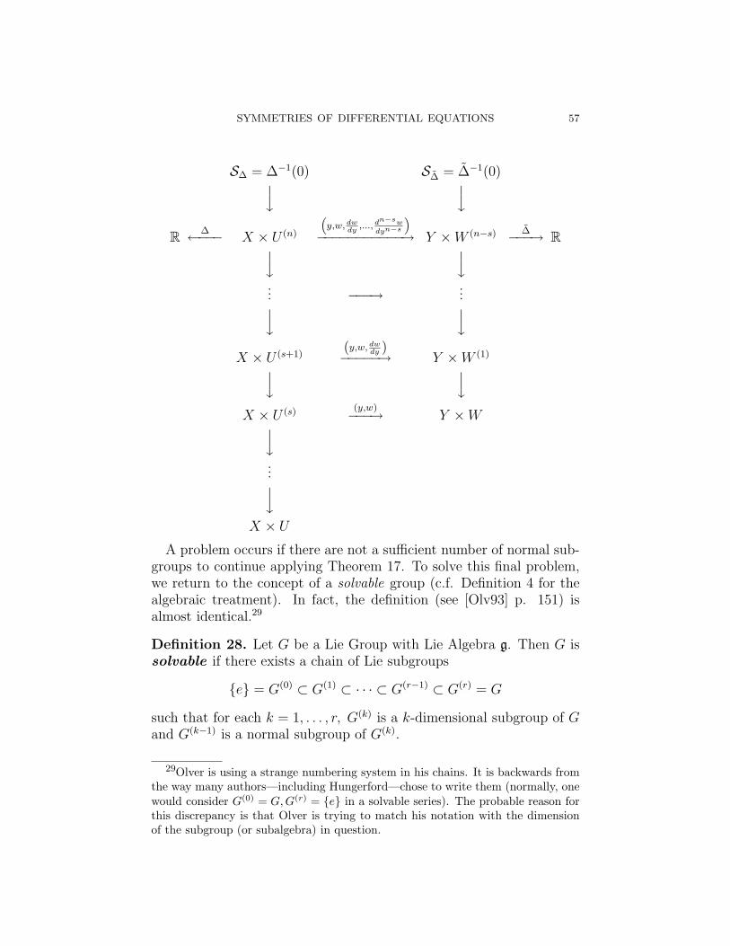
SYMMETRIES OF DIFFERENTIAL EQUATIONS 57
S∆ = ∆−1(0) S∆ = ∆−1(0)y yR ∆←−−− X × U (n)
“y,w, dw
dy,..., dn−sw
dyn−s
”−−−−−−−−−−−→ Y ×W (n−s) ∆−−−→ Ry y
... −−−→ ...y yX × U (s+1)
(y,w, dwdy )
−−−−−→ Y ×W (1)y yX × U (s) (y,w)−−−→ Y ×Wy
...yX × U
A problem occurs if there are not a sufficient number of normal sub-groups to continue applying Theorem 17. To solve this final problem,we return to the concept of a solvable group (c.f. Definition 4 for thealgebraic treatment). In fact, the definition (see [Olv93] p. 151) isalmost identical.29
Definition 28. Let G be a Lie Group with Lie Algebra g. Then G issolvable if there exists a chain of Lie subgroups
e = G(0) ⊂ G(1) ⊂ · · · ⊂ G(r−1) ⊂ G(r) = G
such that for each k = 1, . . . , r, G(k) is a k-dimensional subgroup of Gand G(k−1) is a normal subgroup of G(k).
29Olver is using a strange numbering system in his chains. It is backwards fromthe way many authors—including Hungerford—chose to write them (normally, onewould consider G(0) = G, G(r) = e in a solvable series). The probable reason forthis discrepancy is that Olver is trying to match his notation with the dimensionof the subgroup (or subalgebra) in question.

58 JACOB HARRY BURKMAN
There are several equivalent ways that we can express this concept,dealing with the Lie algebra and vector fields. For instance, we canequivalently say that there exists a chain of subalgebras
0 = g(0) ⊂ g(1) ⊂ · · · ⊂ g(r−1) ⊂ g(r) = g
such that for each k, dim g(k) = k and g(k−1) is a normal subalgebra ofg(k), i.e. [g(k−1), g(k)] ⊂ g(k−1). Furthermore, we could also consider itto be equivalent to the existence of a basis v1, . . . ,vr of g such that
[vi,vj] =
j−1∑k=1
ckijvk, whenever i < j.
As a note, clearly we have that any abelian Lie algebra is solvable(this makes sense since any abelian group is solvable). “Also every twodimensional Lie algebra is solvable. The simplest Lie algebra that isnot solvable is the three-dimensional algebra sl(2), the Lie algebra ofSL(2).”30
We are about to finally arrive at the fruits of our labor. We soughta connection between the Abstract Algebra result that solvability ofthe Galois group leads to the polynomial equation being solvable byradicals (c.f. Theorem 5) and the result in the Lie version of Differen-tial Equations that an equation admitting a solvable symmetry groupleads to the equation being solvable by quadrature (c.f. Theorem 20).However, as in the case with the result in Abstract Algebra, we willbootstrap our way to this result, starting with an elementary proposi-tion.
Proposition 7. Suppose that G is a two-parameter group with a non-abelian Lie algebra g. There there exists a basis v,w for g such that[v,w] = v.
Proof. Suppose that G is a two-parameter group with non-abelian Liealgebra g having basis e1, e2. Since g is not abelian, we may define
v = [e1, e2] 6= 0.
Furthermore, since e1, e2 form a basis, we can write
v = ae1 + be2, a2 + b2 6= 0.
Now let w = −be1 + ae2.
30See [Olv93] p. 151.

SYMMETRIES OF DIFFERENTIAL EQUATIONS 59
Then it is clear that the matrix of coefficients is not singular; there-fore, v, w forms a basis for g. Furthermore, by Equation (11), wecan see that
[v, w] = (a2 + b2)v.
Now, if we let w = 1a2+b2
w,v = v, we see that indeed
[v,w] = v.
We begin with the simple case (see [Olv93] p. 149)–recalling that all2-parameter Lie groups are solvable.
Theorem 19. Let ∆(x, u(n)) = 0 be an nth order ordinary differentialequation invariant under a two-parameter (and hence solvable) symme-
try group G. Then there is an (n−2)nd order equation ∆(z, v(n−2)) = 0with the property that the general solution to ∆ can be found by a pairof quadratures from the general solution to ∆.
Proof. Let ∆(x, u(n)) = 0 be an nth order differential equation that hasa two-parameter symmetry group G. Then, by Proposition 7, we canfind a basis v,w for g with the property that
[v,w] =
0 if g is abelian,
v otherwise.
This result shows us that [v,w] ⊂ Spanv. Hence the one-parametersubgroup H generated by v is a normal subgroup of G (see Proposi-tion 6), with one-parameter quotient group G/H. To effect the reduc-tion of ∆, we begin by determining first order differential invariantsy = η(x, u), w = ζ(x, u, ux) for H using our earlier methods. By The-orem 17, our nth order equation is equivalent to an (n − 1)st orderequation
∆(y, w(n−1)) = 0;
moreover, once we know the solution w = h(y) of this latter equation,we can reconstruct the solution to ∆ by solving
ζ(x, u, ux) = h(η(x, u)
)with a single quadrature.
Since H is normal, by Theorem 18, the reduced equation ∆ is in-variant under the action of G/H on the variables (y, w), and hence wecan employ our earlier methods for one-parameter symmetry groups toreduce the order yet again by one to
60 JACOB HARRY BURKMAN
∆
(z, v,
dv
dz, . . . ,
dn−2v
dzn−2
)= 0.
Now, suppose that we can find a solution v = g(z) of ∆ = 0. Thenby Theorem 17, we can construct a solution w = h(y) of ∆ by a singlequadrature from v(y, w, wy) = g(z(y, w)). But as noted above, once we
have a solution of ∆, we can find a solution u = f(x) for ∆ by a single
quadrature. Thus we can go from a solution of ∆ to a solution of ∆by two quadratures.
Before we can get to the final result, we need to cover one other idea(see [Olv93] p. 147). Let G be an r-parameter Lie Group acting on anm-dimensional manifold, M . Suppose that H is an s-parameter normalsubgroup of G with η(x) = (η1(x), . . . , ηm−s(x)) forming a complete setof functionally independent invariants. Then there is an induced actionof G on M ⊂ Rm−s having invariants y = (y1, . . . , y(m−s)) = η(x). Notethat H clearly will act trivially on the set M . Furthermore, we can,in an essentially arbitrary manner, complete the coordinate system onM by adjoining to the set y further variables x = (x1, . . . , xs), givingus a coordinate system (y, x) for M . Therefore, by making use ofProposition 6, we have that each infinitesimal generator of G must beof the form
(60) vk =m−s∑i=1
ηik(y)
∂
∂yi+
s∑j=1
ξjk(y, x)
∂
∂xj
in the coordinates (y, x). Furthermore, in these coordinates ηi is inde-pendent of the parametric variables x. Since H acts trivially on M , vk
reduces to
vk =s∑
i=1
ηik(y)
∂
∂yi,
which is a well defined vector field generating the reduced action of Gon M .
We are now ready to state and prove the final major result (see[Olv93] p. 151-152).
Theorem 20. Let ∆(x, u(n)) = 0 be an nth order ordinary differentialequation. If ∆ admits a solvable r-parameter group of symmetries Gwith subnormal series G(0) < G(1) < · · ·G(r) as in Definition 28 suchthat for 1 ≤ k ≤ r the orbits of pr(k)G(k) have dimension k, then

SYMMETRIES OF DIFFERENTIAL EQUATIONS 61
the general solution of ∆ can be found by quadratures from the generalsolution of an (n− r)th order differential equation ∆(y, w(n−r)) = 0. Inparticular, if ∆ admits an n-parameter solvable group of symmetries,then (subject to the above technical restrictions), the general solutionto ∆ can be found by quadratures alone.
Proof. The proof proceeds by induction along the chain of subalgebrasin the equivalent condition of solvability (that is that there exists aseries of subnormal algebras g(0) ⊂ g(1) ⊂ · · · ⊂ g(k) ⊂ g(k+1) ⊂ · · · ⊂g(r)) of G (c.f. Definition 28). The initial stage of the induction ar-gument was Theorem 19. Now assume the induction hypothesis: thatthe result of the theorem holds for the kth stage. In other words, wehave that ∆ is invariant under the k-dimensional subalgebra g(k); thus,it can be reduced to an (n− k)th order equation
∆(k)(y, w(n−k)) = 0
in which y, w, dwdy, . . . , dn−kw
dyn−k form a complete set of functionally inde-
pendent differential invariants for the nth prolongation pr(n)G(k); inparticular, y = η(x, u(k)), w = ζ(x, u(k)) form a complete set of invari-ants of the kth prolongation of G(k). (Recall that we are assuming thatthe orbits of G(k) are k-dimensional.) Furthermore, we also assumethat we can construct the general solution u = f(x) from the generalsolution w = h(y) of ∆(k) by a series of k quadratures.
We must now show that the result holds for the (k + 1)st stage. Inorder to do this, consider a generator vk+1 of g(k+1) which does not liein g(k). Since g(k) is a normal subalgebra (in other words, an ideal) ofg(k+1), pr(k) vk+1 takes the form (see Equation 60)
pr(k) vk+1 = pr(k−2) vk+1+α(y, w)∂
∂y+ψ(y, w)
∂
∂w≡ pr(k−2) vk+1+vk+1
in which pr(k−2) vk+1 depends on the non-invariant coordinates x, u, . . . ,uk−2 needed to complete y, w to a coordinate system on M (k). (Onecan further see this by assuming that the coordinates can be selected inthat manner, and then seeing that all of the functions of the first k− 2prolongations do not change with the change of variables. The onlyplace there is something happening is with the coefficient functions of∂y, ∂w.)
Then, Theorem 18 says (if we interpret it in terms of infinitesimals)that the original equation ∆ is invariant under all of g(k+1) if and onlyif the reduced equation ∆(k) is invariant under the reduced vector fieldvk+1 which allows us to implement our reduction procedure for ∆(k)

62 JACOB HARRY BURKMAN
using the vector field vk+1. Namely, we set
y = η(y, w), w = ζ(y, w, wy)
to be independent invariants of the first prolongation pr(1) vk+1. Then
y, w, dwdy, . . . , dn−k−1w
dyn−k−1 form a set of invariants for the (n−k)th prolonga-
tion pr(n−k) vk+1. Since ∆(k) determines an invariant subvariety of thisgroup, there is an equivalent equation
∆(k+1)(y, w(n−k−1)) = 0
depending only on the invariants of pr(n−k) vk+1. Moreover, to recon-
struct the solutions to ∆(k) from those, w = h(y), to ∆(k+1), we needonly solve the first order equation
ζ(y, w, wy) = h(η(y, w)
).
This is invariant under the one-parameter group generated by vk+1
and hence can be integrated by quadrature. This completes the induc-tion step, and thus the proof to the theorem.
We close this by considering an example.
Example 15. 31 Consider the third order equation
(61) u5xuxxx = 3u4
xu2xx + u3
xx.
There is a three-parameter group of symmetries, generated by thevector fields
v1 =∂
∂u, v2 =
∂
∂x, v3 = u
∂
∂x.
This group is solvable since
[v1,v2] = 0, [v1,v3] = v2, [v2,v3] = 0,
i.e. its derived algebra is v2 which is abelian.Hence, by Theorem 20, we have that Equation (61) can be solved by
quadratures. First for g(1), which is generated by v1, we have invariantsx, v = ux. (We need to choose the first one so that it is abelian in orderfor the series to be solvable.) Using these invariants, we can reduceEquation (61) to
(62) v5vxx = 3v4v2x + v3
x.
31See [Olv93] p. 152-154.

SYMMETRIES OF DIFFERENTIAL EQUATIONS 63
Now, the vector field v2 maintains its form v2 = ∂∂x
when written
using the invariants of g(1), so to reduce Equation (62), for g(2) =Spanv1,v2 we need the invariants
y = v, w = vx, wy =vxx
vx
,
of pr(2) v2. In terms of these, we can then reduce Equation (62) to thefirst order equation
(63) y5wy = 3y4w + w2.
This is a Ricatti equation. However, in contrast to Example 14,Equation (63) should still retain a symmetry corresponding the vectorfield v3 that we have not yet used in any reduction. Indeed, in termsof x, y = ux, w = uxx,
pr(2) v3 = u∂
∂x− y2 ∂
∂y− 3yw
∂
∂w
and the reduced vector field
v3 = −y2 ∂
∂y− 3yw
∂
∂w
is a symmetry of Equation (63). We now perform a change of variablesin Equation (63) by setting t = −1
y, z = w
y3 . (Here we are essentially
using Theorem 6.) Using this change of variables, we can see thatv3 = − ∂
∂t, and hence reduce Equation (63) to
dz
dt= z2, ⇒ z =
1
c− tfor some constant c. Of course, what we really want is a solution ofthe original Equation (61). In many of the previous examples, workingbackwards was difficult to impossible. However, here we can. If were-express the previous in terms of the invariants of v2,
w =y4
cy + 1.
Now, going farther back to find v, we need to solve the autonomous(and separable) equation
dv
dx=
v4
cv + 1.
From this, we can find an implicit solution for v = ux.
6(x− k)v3 + 3cv + 2 = 6(x− k)u3x + 3cux + 2 = 0
where k is another constant of integration.

64 JACOB HARRY BURKMAN
We then solve the above equation for ux. This is not direct, andmay be very difficult (but remember there is a general form for a cubicequation), but once we do, we have reduced the solution of Equation(61) to quadrature.
Before we close, several comments should be made about the resultsof the previous example. First of all, note that it is possible for asymmetry to disappear and then reappear. Note that there is no cor-responding symmetry to v3 for Equation (62). Therefore, we have that“in the general reduction procedure, it is important to wait until wehave the invariants for g(k) before trying to reduce the next vector fieldvk+1; one cannot expect vk+1 to naturally reduce relative to an earliersubalgebra g(j) if j < k.”32
32See [Olv93] p. 154.

SYMMETRIES OF DIFFERENTIAL EQUATIONS 65
8. Differential Galois Theory and Picard-VissiotExtensions
Recall, from Abstract Algebra, and from Section (1), the basics ofGalois Theory for polynomial equations. Here we establish a slightparallel with differential equations. Let R denote a commutative ring(often we will actually want a field). We then can define the following(see [San98] p. 58).
Definition 29. An additive map d : R→ R is called a derivation ifd satisfies the Leibnitz rule, namely that d(ab) = a · d(b) + d(a) · b.
If R is actually an integral domain, then we can extend it to its fieldof quotients K and extend the map d to a map d : K → K (where wefollow the traditional notation of referring to the extension by the samename) that obeys something similar to the quotient rule. Of course, ifR is actually a field, R is its own field of quotients. Once we have this,we can define the following.
Definition 30. The pair (K, d) described above is called a differen-tial field .
Now, let L = Y (n) +a1Y(n−1) + · · ·+anY
(0) be a differential operatorwhere the aj ∈ (F, d) (where F is a field).
Notation 9. We denote by FY the adjoining to F a differentialindeterminate Y .
(The reader should recognize this is similar to the notation estab-lished for the polynomial ring R[x].)
We are now ready to define a Picard-Vessiot extension (see [San98]p. 61-62).
Definition 31. Let (F, d) be a differential field and let L ∈ FY bea monic linear homogeneous differential operator. A differential fieldextension E of F is said to be a Picard-Vessiot extension of Ffor L, if the following are satisfied.
(1) The field of constants of F is the same as the field of constantsof E.
(2) E is generated over F by the vector space V of all solutions ofL = 0 in E.
(3) E contains a full set of solutions to the differential equationL = 0. In other words, there exist yi, i = 1, 2, . . . , n where n isthe order of L in V such that the Wronskian of y1, y2, . . . , yn isnot zero.
66 JACOB HARRY BURKMAN
(Again the reader should have some inkling that this definition issimilar to an extension of a polynomial ring up to the splitting field ofsome polynomial over that ring.)
With one more definition (that of a linear algebraic group), we canestablish the Fundamental Theorem of Differential Galois Theory (see[Mag99] p. 1043).
Definition 32. A linear algebraic group over C is a subgroup ofsome general linear group GLn(C) that is the zero locus of a set ofpolynomials in the matrix entries.
Theorem 21. Fundamental Theorem of Differential Galois The-ory: Let E ⊃ F be a Picard-Vessiot extension with common alge-braically closed field C as the field of constants of both E and F . LetG be a group of differential automorphisms of E over F . Then G hasstructure of a linear algebraic group over C, and there is a one-to-oneinclusion reversing correspondence between the intermediate differen-tial field extensions E ⊃ K ⊃ F and closed subgroups H of G, with Kcorresponding to
g ∈ G|g(k) = k for all k ∈ Kand H corresponding to
x ∈ E|h(x) = x for all h ∈ H.Moreover, H is a normal subgroup of G if and only if the corre-
sponding extension K is a Picard-Vessiot extension of F , and if so,then the group of differential automorphisms of K over F is identifiedwith G/H.
Of course, a reader familiar with the Fundamental Theorem of GaloisTheory (c.f. Theorem 1) should see that these theorems are basicallyidentical, with the group mentioned being the Galois Group in Theorem1, and the differential Galois group in Theorem 21. The choice ofthis name is “appropriate and historical, Lie having pointed out theanalogy in 1895.” 33 This connects back to differential equations for“the solvability of this group is then a necessary and sufficient conditionfor the [differential] equation to be solvable by quadratures.”34
33See [Mag99] p. 1043.34See [Hel94] p. 18.

SYMMETRIES OF DIFFERENTIAL EQUATIONS 67
9. Conclusion
We have seen that Sophus Lie, in his somewhat unique view of differ-ential equations, created a means to examine the differential equationsin a method that is not very familiar. Using this method of symme-tries we are able to examine the differential equations and their solu-tions in a new light by obtaining an understanding of the underlyingspace. However, despite the seeming utility of this method, we haveseen that the process of calculating the symmetries can become verycumbersome—perhaps this is why we are not as familiar with themas we are with the other methods that we have all seen in differentialequations classes. However, exploring this method, has provided a newinsight into differential equations and a better understanding of whatis occurring in them. Furthermore, we have reached one of the majorconnections between differential equations and abstract algebra—onethat is not commonly emphasized. This connection is related to thesolvability of the equation. In the case of abstract algebra, we have theresult that the polynomial equation is solvable by radicals if and only ifthe Galois group of the polynomial is a solvable group. The differentialequation result is that if the equation admits a solvable group, then itis solvable by quadratures.
The field that Sophus Lie began as an attempt to better understanddifferential equations is one that has branched greatly. We have barelytouched on all of the aspects here. Lie’s “group” (what today we wouldcall a Lie Algebra), and the real group that we call a Lie Group havebecome fundamental subjects in their own right. There are many math-ematicians studying these topics (and making new discoveries) today.(Several have been cited herein: Peter Olver at the University of Min-nesota, Sigurdur Helgason at MIT, and Thomas Hawkins at BostonUniversity.) In the interest of not having too many sources say thesame thing, and to keep this from becoming a real book, we have, how-ever, focused primarily on those found in Olver. Other sources includeworks by Peter Hydon from the University of Surrey and Hans Stephaniat Friedrich-Schiller-Universitat dealing with differential equations andtheir symmetries. The text mentioned by Bluman in the bibliographyis also an excellent work on this topic (which is more readable thanOlver). While we just mentioned it very briefly, the field of differentialGalois Theory is also a large field, with recent and authoritative worksby Andy Magid at the University of Oklahoma and J.F. Pommaret, theDocteur es-Sciences Ancien eleve de l’Elcole Polytechnique Ingenieur

68 JACOB HARRY BURKMAN
des Ponts et Chaussees. So, needless to say, we have seen the classi-cal underpinnings of this theory, and there is definitely modern workcontinuing on many of the topics that are a result of Sophus Lie’s ideefixe.

SYMMETRIES OF DIFFERENTIAL EQUATIONS 69
References
[BC96] David Bleecker and George Csordas, Basic partial differential equations,International Press, Cambridge, MA, 1996. MR MR1606155 (98m:35001)
[BD97] William E. Boyce and Richard C. DiPrima, Elementary differential equa-tions and boundary value problems, sixth ed., John Wiley & Sons Inc.,New York, 1997. MR MR0179403 (31 #3651)
[BK89] George W. Bluman and Sukeyuki Kumei, Symmetries and differentialequations, Applied Mathematical Sciences, vol. 81, Springer-Verlag, NewYork, 1989. MR MR1006433 (91b:58284)
[Haw00] Thomas Hawkins, Emergence of the theory of Lie groups, Sources andStudies in the History of Mathematics and Physical Sciences, Springer-Verlag, New York, 2000, An essay in the history of mathematics 1869–1926. MR MR1771134 (2001f:01031)
[Hel90] Sigurdur Helgason, Sophus Lie and the role of Lie Groups in Mathematics,Report of the 14. Nordic LMFK-Conference (Reykjavik), 1990.
[Hel94] , Sophus Lie, the mathematician, The Sophus Lie MemorialConference (Oslo, 1992), Scand. Univ. Press, Oslo, 1994, pp. 3–21.MR MR1456457 (98g:01061)
[Hun80] Thomas W. Hungerford, Algebra, Graduate Texts in Mathematics,vol. 73, Springer-Verlag, New York, 1980, Reprint of the 1974 original.MR MR600654 (82a:00006)
[Hyd00] Peter E. Hydon, Symmetry methods for differential equations, CambridgeTexts in Applied Mathematics, Cambridge University Press, Cambridge,2000, A beginner’s guide. MR MR1741548 (2001c:58036)
[Mag99] Andy R. Magid, Differential Galois theory, Notices Amer. Math. Soc. 46(1999), no. 9, 1041–1049. MR MR1710665 (2001c:12007)
[Olv93] Peter J. Olver, Applications of Lie groups to differential equations, seconded., Graduate Texts in Mathematics, vol. 107, Springer-Verlag, New York,1993. MR MR1240056 (94g:58260)
[OR] J. J. O’Connor and E.F. Robertson, Marius Sophus Lie, on-line http://www.history.mcs.st-andrews.ac.uk/Biographies/Lie.html, Ac-cessed on 11/21/06.
[San98] N. Sankaran, Galois theory of differential fields—a survey, Bull. AllahabadMath. Soc. 12/13 (1997/98), 57–83. MR MR1761034 (2001f:12010)
Department of Mathematics, University of Hawai‘i at Manoa, Hon-olulu, HI 96822
E-mail address: [email protected]