Commun. Theor. Phys. (Beijing, China) 51 (2009) pp. 973–978c© Chinese Physical Society and IOP Publishing Ltd Vol. 51, No. 6, June 15, 2009

Symmetry and Exact Solutions of (2+1)-Dimensional Generalized Sasa–Satsuma

Equation via a Modified Direct Method∗

LU Chang-Cheng1 and CHEN Yong1,2,†

1Nonlinear Science Center and Department of Mathematics, Ningbo University, Ningbo 315211, China

2Shanghai Key Laboratory of Trustworthy Computing, East China Normal University, Shanghai 200062, China

(Received May 19, 2008)

Abstract In this paper, first, we employ classic Lie symmetry groups approach to obtain the Lie symmetry groupsof the well-known (2+1)-dimensional Generalized Sasa–Satsuma (GSS) equation. Second, based on a modified directmethod proposed by Lou [J. Phys. A: Math. Gen. 38 (2005) L129], more general symmetry groups are obtained andthe relationship between the new solution and known solution is set up. At the same time, the Lie symmetry groupsobtained are only special cases of the more general symmetry groups. At last, some exact solutions of GSS equationsare constructed by the relationship obtained in the paper between the new solution and known solution.

PACS numbers: 02.30.JrKey words: classic Lie symmetry groups approach, modified CK’s direct method, generalized Sasa–Satsuma

equation

1 IntroductionLie symmetry is one of the most powerful methods

in every branch of natural science especially in integrablesystems.[1,2,3] To find the Lie point symmetry group ofa nonlinear system, there is a standard method to findsymmetry algebras and groups for almost all the knownintegrable systems. In previous paper,[4] Clarkson andKruskal (CK) introduced a simple direct method to de-rive symmetry reductions of a nonlinear system withoutusing any group theory. For many types of nonlinear sys-tems, those symmetry gained by CK’s direct method canalso be generated via the classical and nonclassic Lie groupapproach.[5] In previous paper,[6] the conditional similar-ity reducation solution can also be obtained by the mod-ified CK’s direct method. These facts hint that there isa simple method to find generalized symmetry groups formany types of nonlinear equations.

In this paper, we consider the Generalized Sasa–Satsuma (GSS) equation,[7] which has this following form:

∆1 ≡ qt + qxxx + 6qxU + 3qUx = 0 , (1)

∆2 ≡ rt + rxxx + 6rxU + 3rUx = 0 , (2)

∆3 ≡ Uy − (qr)x = 0 , (3)

and is a generalization of the Sasa–Satsuma equation in-troduced recently:[8]

qt + qxxx + 6qxU + 3qUx = 0 , (4)

Uy − (|q|2)x = 0 , (5)

where q is the complex physical field and U is the real po-tential for Eqs. (1)–(3). When r is taken as the complexconjugate of q, Eqs. (1)–(3) become the Eqs. (4) and (5).

This paper is arranged as follows: In Sec. 2, first, with

the method of classic Lie group, the Lie point symmetry

of GSS equation can be obtained, then by using the modi-

fied direct method, we get a relationship between the new

solution and known solution of the GSS equation. Taking

some special case, the Lie symmetry of the GSS equation

also can be gained, by solving the corresponding charac-

teristic equation, then the reduced equations can be ob-

tained. In Sec. 3, some explict solutions of GSS equation

are presented via choosing different parameters. Finally,

some conclusions and discussions are given in Sec. 4.

2 Symmetry and Reduction of GSS Equation

In this section, we look for the symmetry of

Eqs. (1)–(3) by using the classical Lie method. Let us

consider a one-parameter Lie group of infinitesimal trans-

formation

x → x + εξ(x, u, t, q, r, U) ,

y → y + εη(x, u, t, q, r, U) ,

t → t + ετ (x, u, t, q, r, U) ,

q → q + εφ1(x, u, t, q, r, U) ,

r → r + εφ2(x, u, t, q, r, U) ,

U → U + εφ3(x, u, t, q, r, U) ,

with a small parameter ε, the corresponding vector field

associated with the above group of transformations to GSS

equation can be written as

V = ξ∂

∂x+ η

∂

∂y+ τ

∂

∂t+ φ1

∂

∂q

∗Supported by the National Natural Science Foundation of China under Grant No. 10735030, Shanghai Leading Academic Discipline

Project under Grant No. B412, National Natural Science Foundation of China under Grant No. 90718041, Program for Changjiang Scholars

and Innovative Research Team in University under Grant No. IRT0734 and K.C. Wong Magna Fund in Ningbo University†E-mail: chenyong@nbu.edu.cn

974 LU Chang-Cheng and CHEN Yong Vol. 51

+ φ2∂

∂r+ φ3

∂

∂U,

where ξ, η, τ , φ1, φ2, and φ3 are the funcations with

respect to {x, y, t, q, r, U}, the prolongation of the vector

field is

pr(3)V = V + φx1

∂

∂qx+ φt

1

∂

∂qt+ φxxx

1

∂

∂qxxx+ φx

2

∂

∂rx

+ φt2

∂

∂qt+ φxxx

2

∂

∂rxxx+ φx

3

∂

∂Ux+ φy

3

∂

∂Uy,

where

φx1 = Dx(φ1 − ξqx − ηqy − τqt)

+ ξqxx + ηqxy + τqxt ,

φt1 = Dt(φ1 − ξqx − ηqy − τqt)

+ ξqxt + ηqyt + τqtt ,

φxxx1 = Dxxx(φ1 − ξqx − ηqy − τqt)

+ ξqxxxx + ηqxxxy + τqxxxt ,

φx2 = Dx(φ2 − ξrx − ηry − τrt)

+ ξrxx + ηrxy + τrxt ,

φt2 = Dt(φ2 − ξrx − ηry − τrt)

+ ξrxt + ηryt + τrtt ,

φxxx2 = Dxxx(φ2 − ξrx − ηry − τrt)

+ ξxxxx + ηrxxxy + τrxxxt ,

φx3 = Dx(φ3 − ξUx − ηUy − τUt)

+ ξUxx + ηUxy + τUxt ,

φy3 = Dy(φ3 − ξUx − ηUy − τUt)

+ ξUxy + ηUyy + τUyt .

By using these extensions and applying the prolonga-

tion to the GSS equation, the infinitesimal criteria for the

invariance of Eqs. (1)–(3) under the group is given by

pr(3)V∆i|∆j=0 = 0 (i, j = 1, 2, 3) . (6)

After substituting Eqs. (1)–(3) into Eq. (6) for i, j =

1, 2, 3, comparing the coefficients of linearly independent

expressions of {q, r, U} and let their derivatives be zero

(qt, rt, Uy and their derivatives have been cancelled by ∆i

(i = 1, 2, 3)), we obtain various constraint equations. And

solving these equations, one can obtain

ξ =F1(t)x

3+ F4(t), η = F2(y), τ = F1(t) ,

φ1 = −1

6q(6F2(y) + F1(t) + 6F3(y)) ,

φ2 =(

− F1(t)

6+ F3(y)

)

r ,

φ3 =F1(t)

18x +

F4(t)

6− 2F1(t)

3U .

If we want to obtain the relation between the new so-

lution and known solution of GSS equation, one has to

solve the following ODEs

dx

dε= ξ(x, y, t, q, r, U) ,

dy

dε= η(x, y, t, q, r, U) ,

dt

dε= τ (x, y, t, q, r, U) , (7)

dq

dε= φ1(x, y, t, q, r, U) ,

dr

dε= φ2(x, y, t, q, r, U) ,

dU

dε= φ(x, y, t, q, r, U) , (8)

with initial solution conditions

x|ε=0 = x, y|ε=0 = y, t|ε=0 = t ,

q|ε=0 = q, r|ε=0 = r, U |ε=0 = U . (9)

Solving the Eqs. (7)–(9) is difficult,[9] because the

equations inclued some arbitrary functions, such as F1(t),

F4(t), F2(y), F3(y). If we want to get the transforma-

tion between the new solution and known solution of GSS

equation, one may use the modified direct method.

For the GSS equation, in order to search the trans-

formation between the new solution and known solution,

it is enough to seek the symmetry reductions in a simple

form[10]

q = α + βQ(ξ, η, τ) , (10)

r = γ + θR(ξ, η, τ) , (11)

U = ζ + φW (ξ, η, τ) , (12)

where α = α(x, y, t), β = β(x, y, t), γ = γ(x, y, t),

θ = θ(x, y, t), ζ = ζ(x, y, t), φ = φ(x, y, t) and ξ, η, τ

are functions of {x, y, t} to be determined later, under the

transformations

{x, y, t, q(x, y, t), r(x, y, t), U(x, y, t)}→ {ξ, η, τ, Q(ξ, η, τ), R(ξ, η, τ), W (ξ, η, τ)} ,

and satisfy the same PDEs

Qτ + Qξξξ + 6QξW + 3QWξ = 0 , (13)

Rτ + Rξξξ + 6RξW + 3RWξ = 0 , (14)

Wη − (QR)ξ = 0 . (15)

Substituting Eqs. (10)–(12) along with Eqs. (13)–(15)

into Eqs. (1)–(3) and eliminating Qτ , Rτ , Wη and their

higher order derivatives by means of the Eqs. (13)–(15).

Let the coefficients of U , V , W and their derivatives be

zero, we arrive at some PDEs which are omitted in this

paper. By solving the above PDEs, we have the following

results:

ξ = f1(t)2x − 6

∫

f2(t)f1(t)dt ,

η =

∫

f3(y)f4(y)dy ,

τ =

∫

f1(t)6dt, α = 0, γ = 0 ,

β = f3(y)f1(t), θ = f4(y)f1(t) ,

ζ = − f1(t)x

3f1(t)+ f2(t), φ = f1(t)

4 .

No. 6 Symmetry and Exact Solutions of (2+1)-Dimensional Generalized Sasa–Satsuma Equation · · · 975

In summary, by using Eqs. (10)–(12), the following theo-

rem holds:

Theorem 1 If Q(ξ, η, τ), R(ξ, η, τ), W (ξ, η, τ) are the

solutions of the GSS equation, then the GSS equation also

has solutions as follow:

q(x, y, t) = f3(y)f1(t)Q(ξ, η, τ) ,

r(x, y, t) = f4(y)f1(t)R(ξ, η, τ) ,

U(x, y, t) = − f1(t)

3f1(t)x + f2(t) + f1(t)

4W (ξ, η, τ) .

To obtain the Lie point symmetry group obtained from

Theorem 1, we restrict:

f1(t) = 1 + εf(t), f2(t) = εF2(t) ,

f3(y) = 1 + εF3(y), f4(y) = 1 + εF4(y)

with an infinitesimal parameter ε, then equations in The-

orem 1 can be written as:

q = Q + εδ(Q), r = R + εδ(R), U = W + εδ(W ) .

Furthermore if setting

f(t) =F1(t)

6, f2(t) = −H4(t)

6,

f3(y) + f4(y) = G4(y) ,

we also obtain the symmetry

δ(q) =( F1(t)x

3+ H4(t)

)

Qx + G4(y)Qy

+ F1(t)Qt +( F1(t)

6+ F3(y)

)

Q , (16)

δ(r) =( F1(t)x

3+ H4(t)

)

Rx + G4(y)Ry

+ F1(t)Rt +( F1(t)

6+ F4(y)

)

R , (17)

δ(U) =( F1(t)x

3+ H4(t)

)

Wx + G4(y)Wy

+ F1(t)Wt −F1(t)x

18− H4(t)

6

+2F1(t)

3W . (18)

If one set some constraint conditions, the Eqs. (16)–

(18) are equal to the vector field obtained by classic Lie

point group.

The solutions of Eqs. (16)–(18) are obtained by solving

the characteristic equation,[5] then one obtain the similar-

ity form of the solution as

q = F1(x, y, t, Φ1(X, Y )) ,

r = F2(x, y, t, Φ2(X, Y )) ,

U = F3(x, y, t, Φ3(X, Y )) , (19)

where X and Y are similarity variables, the others

Φ1(X, Y ), Φ2(X, Y ), Φ3(X, Y ) are dependent variables.

Substituting Eqs. (19) into Eqs. (1)–(3), then we can ob-

tain the reduction equations of GSS equation.

By setting F1(t) = t, H4(t) = t, G4(y) = y, F3(y) = 0,

F4(y) = 1 as an example, the invariant surface conditions

become(x

3+ t

)

Qx + yQx + tQx +1

6Q = 0 , (20)

(x

3+ t

)

Rx + yRx + tRx +7

6Q = 0 , (21)

(x

3+ t

)

Wx + yWx + tWx − 1

6+

2

3W = 0 . (22)

The corresponding characteristic equation is

dx

x/3 + t=

dy

y=

dt

t=

dq

−1/6=

dr

−7/6

=dW

1/6 − (2/3)W. (23)

Solving the characteristic Eq. (23), we obtain

q = t7/6Φ1(X, Y ), r = t1/6Φ2(X, Y ) ,

U =1

5t + t−2/3Φ3(X, Y ) , (24)

X =5x − 3t2

5t1/3, Y =

y

t. (25)

Substituting Eqs. (24) and (25) into Eqs. (1)–(3), the re-

duction of GSS equation read

7Φ1 + 2XΦ1X + 6Y Φ1Y − 6Φ1XXX

− 36Φ1XΦ3 − 18Φ1Φ3X = 0 , (26)

Φ2 + 2XΦ2X + 6Y Φ2Y − 6Φ2XXX

− 36Φ2XΦ3 − 18Φ2Φ3X = 0 , (27)

Φ3Y − Φ1XΦ2 − Φ2XΦ1 = 0 . (28)

As we see, the reduced GSS equation are still complex

and to solve the Eqs. (26)–(28) is difficult. However, the

above results and discussion set up the relations between

new and the known solution, which can construct new so-

lutions. In addition, the more general symmetry group

are obtained, which include the classical point symmetry

group.

3 Solution of (2+1)-Dimensional GSS Equa-tion

In the paper,[7] the author solve the GSS equation by

the Painleve approach and the final solutions can be given

in terms of arbitrary functions as follow

q = −√

φ2xφ1y

2F (φ1 + φ2), (29)

r =F√

φ2x

φ1 + φ2, (30)

U = − φ22x

2(φ1 + φ2)2+

φ2xx

2(φ1 + φ2)

− φ2t + φ2xxx

6φ2x+

φ22xx

8φ22x

, (31)

where φ2 is an arbitrary function of {x, t} and φ1 and F

are arbitrary functions of y. Also the Eqs. (13)–(15) have

976 LU Chang-Cheng and CHEN Yong Vol. 51

the same form solutions:

Q = −√

φ2ξφ1η

2F (φ1 + φ2), (32)

R =F

√

φ2ξ

φ1 + φ2, (33)

W = −φ2

2ξ

2(φ1 + φ2)2+

φ2ξξ

2(φ1 + φ2)

− φ2τ + φ2ξξξ

6φ2ξ+

φ22ξξ

8φ22ξ

, (34)

where φ2 is an arbitrary function of {ξ, τ} and φ1 and F

are arbitrary functions of η.

Here, applying the symmetry group Theorem 1 on

Eqs. (32)–(34), one can obtain some solutions when the

seed solutions of GSS equation are given,

q = −f3(y)f1(t)

√

φ2ξφ1η

2F (φ1 + φ2), (35)

r = f4(y)f1(t)F

√

φ2ξ

φ1 + φ2, (36)

U = − f1(t)

3f1(t)x + f2(t) − f1(t)

4( φ2

2ξ

2(φ1 + φ2)2− φ2ξξ

2(φ1 + φ2)+

φ2τ − φ2ξξξ

6φ2ξ−

φ22ξξ

8φ22ξ

)

, (37)

where ξ = f1(t)2x − 6

∫

f2(t)f1(t)dt, η =∫

f3(y)f4(y)dy, and τ =∫

f1(t)6dt are given in Sec. 2.

In order to get some explicit results, we choose the arbitrary functions φ1 and φ2 as simple as

φ1 = a3eη, φ2 = a0 + a1e

k1ξ−ω1τ ,

where a0, a1, a3, k1, ω1 are arbitrary constants.

Fig. 1 Plots of the GSS equation given by Eqs. 35(a), 36(b), and 37(c) with parameter choice Eqs. (38) and (39) allat time t = 0.05.

Figure 1 displays the solutions structure of Eqs. (36) and (37), with the parameter selections

a0 = 20, a1 = 20, a3 = −1, k1 = 3, ω1 = −2, k3 = −1

2, (38)

No. 6 Symmetry and Exact Solutions of (2+1)-Dimensional Generalized Sasa–Satsuma Equation · · · 977

f1(t) = cos(t)1/6, f2(t) = 0, f3(y) = 1, f4(y) = y, F (η) = 1 . (39)

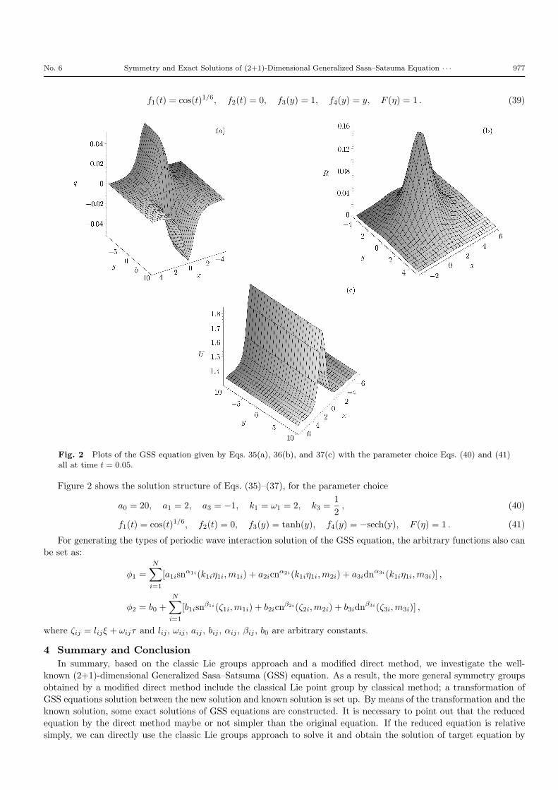
Fig. 2 Plots of the GSS equation given by Eqs. 35(a), 36(b), and 37(c) with the parameter choice Eqs. (40) and (41)all at time t = 0.05.

Figure 2 shows the solution structure of Eqs. (35)–(37), for the parameter choice

a0 = 20, a1 = 2, a3 = −1, k1 = ω1 = 2, k3 =1

2, (40)

f1(t) = cos(t)1/6, f2(t) = 0, f3(y) = tanh(y), f4(y) = −sech(y), F (η) = 1 . (41)

For generating the types of periodic wave interaction solution of the GSS equation, the arbitrary functions also can

be set as:

φ1 =

N∑

i=1

[a1isnα1i(k1iη1i, m1i) + a2icn

α2i(k1iη1i, m2i) + a3idnα3i(k1iη1i, m3i)] ,

φ2 = b0 +

N∑

i=1

[b1isnβ1i(ζ1i, m1i) + b2icn

β2i(ζ2i, m2i) + b3idnβ3i(ζ3i, m3i)] ,

where ζij = lijξ + ωijτ and lij , ωij , aij , bij , αij , βij , b0 are arbitrary constants.

4 Summary and Conclusion

In summary, based on the classic Lie groups approach and a modified direct method, we investigate the well-

known (2+1)-dimensional Generalized Sasa–Satsuma (GSS) equation. As a result, the more general symmetry groups

obtained by a modified direct method include the classical Lie point group by classical method; a transformation of

GSS equations solution between the new solution and known solution is set up. By means of the transformation and the

known solution, some exact solutions of GSS equations are constructed. It is necessary to point out that the reduced

equation by the direct method maybe or not simpler than the original equation. If the reduced equation is relative

simply, we can directly use the classic Lie groups approach to solve it and obtain the solution of target equation by

978 LU Chang-Cheng and CHEN Yong Vol. 51

the transformation between the new solution and the solution of reduced equation. The method reported here can be

applied in principle to all nonlinear systems including both integrable and non-integrable ones and more details will

be reported in future.

References

[1] MA Hong-Cai and LOU Sen-Yue, Commun. Theor. Phys.44 (2005) 193.

[2] P.J. Olver, Application of Lie Group to Differential Equa-

tions, Springer, Berlin (1986).

[3] G.W. Bluman and J.D. Cole, Similarity Methods for

Differential Equations, Applied Mathematical Sciences,Vol. 13, Springer, Berlin (1974).

[4] P.A. Clarkson and M.D. Kruskal, J. Math. Phys. 33

(1989) 2201.

[5] Sen-Yue Lou, J. Math. Phys. 33 (1992) 4300.

[6] Sen-Yue Lou, Xiao-Yan Tang, and Ji Lin, J. Math. Phys.41 (2000) 8286.

[7] R. Radha and S.Y. Lou, Physica Scripta 72 (2005) 432.

[8] C. Gilson, J. Hietarinta, J. Nimmo, and Y. Ohta, Phys.Rev. E 68 (2003) 016614.

[9] D. David, N. Kamran, D. Levi, and P. Winternitz, J.Math. Phys. 27 (1986) 1225.

[10] H.C. Ma, Commun. Theor. Phys. 43 (2005) 1047.