Switchgrass as an Income Stabilizing Crop for Cow-calf Producers Impacted by

Drought

Jennifer Lutes and Michael Popp

J. Lutes and M. Popp are Graduate Research Assistant and Professor in the Department of Agricultural Economics and Agribusiness, University of Arkansas, Fayetteville, AR. Corresponding author is Dr. M. Popp, email: mpopp@uark.edu, ph: 479-575-6838, fax: 479-575-5306 Selected Paper prepared for presentation at the 2015 Agricultural & Applied Economics Association and

Western Agricultural Economics Association Annual Meeting, San Francisco, CA, July 26-28 Copyright 2015 by J. Lutes and M. Popp. All rights reserved. Readers may make verbatim copies of this document for non-commercial purposes by any means, provided that this copyright notice appears on all such copies.

ii

ABSTRACT

Cow-calf producers in Arkansas experience annual fluctuations in their farm returns and are

increasingly scrutinized for their role in climate change. Increasing farm efficiency can increase farm

returns and either increase or decrease net greenhouse gas emissions, but often these practices also

increase income risk. Diversifying enterprise choices, the addition of switchgrass production grown on

converted pasture land, in this case, is thought to lower income risk by providing a drought hardy crop

while at the same time a supply of lignocellulosic biomass for potential bio-refineries. Adopting

rotational grazing, compared to a baseline of continuous grazing, frees pasture acreage to either

increase beef output or to the production of a dedicated energy crop. The objectives are to determine

what switchgrass price is needed to be income neutral and whether adoption of switchgrass does in fact

impact income risk without affecting feed or food supply. Decision support software, the Forage and

Cattle Planner (FORCAP), is used to compare financial returns, along with GHG emissions, across

multiple farm management strategies. The study reveals that the addition of switchgrass production,

when compared to increased beef production, offers lower income risk but the needed switchgrass

price to break even is higher than the price needed to compete with the least intensive continuous

grazing option and lowest stocking rate. Net GHG emissions implications of changes are quite small.

1

Switchgrass as an Income Stabilizing Crop for Cow-calf Producers Impacted by Drought

INTRODUCTION

Cow-calf producers in Arkansas experience annual fluctuations in their farm returns and are

increasingly scrutinized for their role in climate change. Their annual returns are often a reflection of

their reliance on weather, for forage production, and the national cattle supply and demand, for cattle

prices. Many different management practices exist for the purpose of increasing producer efficiency

which may or may not increase returns and or curtail cow-calf production impacts on the environment.

Risk implications of modified management practices on producer returns and greenhouse gas (GHG)

emissions are also an important consideration for producer adoption of alternative management

practices. Diversification of enterprise choices is often a method suggested to decrease overall risk. As

such, a potential diversification approach for cow-calf producers is the addition of growing a

lignocellulosic energy crop for bio-fuel production.

Switchgrass, as a dedicated energy crop, is proposed within as it has a perennial growth habit,

an extensive root system and single fall harvest that make its yield fluctuation due to climatic conditions

from year to year less variable than pasture or hay production, for example. A potential added benefit is

soil carbon sequestration and relative ease of adoption as producers already have the necessary

equipment for harvest. While biofuel, sourced from plant material, is a potentially growing industry in

the United States, this analysis attempts to determine under what conditions beef producers might set

aside some of their pasture acreage to switchgrass production as a dedicated energy crop. At the same

time, enhanced pasture productivity by switching from continuous to rotational grazing is expected to

allow beef output to remain the same. A second risk/return comparison entails an operation that has

changed to rotational grazing and switchgrass production holding beef output constant vs. an operation

2

that also changes to rotational grazing but uses the added efficiency to increase beef production rather

than diversifying to switchgrass.

The objectives of this paper are thus to determine if switchgrass, grown on pastures, would

serve the following purposes: i) to increase supply for alternative energy production without affecting

feed or food supply and at what switchgrass price; ii) provide motive for cattle producers to enhance

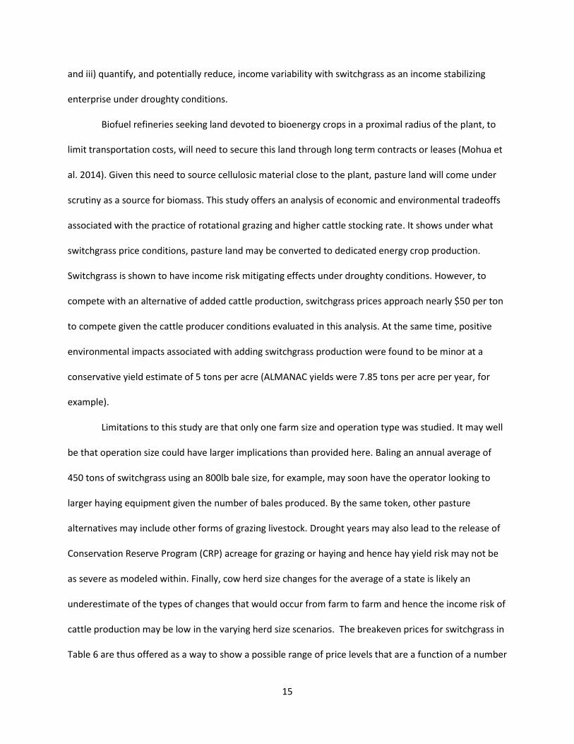
pasture use efficiency; and iii) quantify, and potentially reduce, income variability with switchgrass as an

income stabilizing enterprise under droughty conditions.

LITERATURE REVIEW

Beef Cattle Production

Beef cattle production methods tend to vary across climatic regions given differences in forage

type and seasonal availability. This study focuses on a production region in northwest Arkansas given

access to both warm season and cool season grasses with significant annual rainfall but also high

likelihood of summertime drought. Management of forage resources is thus key to limiting the amount

of costly hay feeding during the production season. This topic has received significant attention with

extension efforts targeting an extended grazing season (Jennings and Jones, n.d.). To enhance pasture

use efficiency, recommendations range from rotational grazing, to stockpiling fescue or bermudagrass,

to fertilizing based on soil testing, to over seeding legumes, to planting winter forages, to harvesting

excess forage for hay, and to reducing hay waste during storage and feeding. The focus of these

recommendations is to increase producer returns by increasing farm efficiency and such strategy

recommendations are common throughout the southeastern U.S.

Different stocking rate strategies have also been offered as a means to mitigate drought risk to

cow-calf producers. One of the main problems cow-calf producers face is an uneven, seasonal growing

pattern of forages. Many farms face dormant forage in the winter, excessive forage in late spring and

3

early summer, and barely sufficient forage to meet cattle nutrient needs in late summer and fall.

Producers often harvest the excess forage in spring for late summer and winter feeding. Varying

stocking rates to match available forage is thus a method to reduce excess forage. Torell, Murugan and

Ramirez (2010) studied the economics of flexible versus conservative stocking rates as a way to mitigate

drought risk. They determined that a conservative cow-calf stocking rate along with a flexible feeder calf

stocking rate would assist producers with managing the whole farm under both drought and non-

drought conditions. However, this also exposes the producer to additional risk due to the fluctuations in

cattle prices associated with buying and selling of feeder cattle. Stocking rate also has implications on

GHG emissions. A study in Texas found more efficient farms produce less GHG emission per unit of beef

produced and per hectare than less efficient farms (Wang et al., 2013). Zilverberg et al. (2011) studied

energy use per cow and per hectare and recommended use of locally adapted forages with high N

efficiency, and replacement of feeding hay with grazing unfertilized dormant forage to reduce cow-calf

energy use. The literature demonstrates that the use of intensive pasture management requires less

land and promotes positive environmental and economic changes on cow-calf farms.

Switchgrass Production

Switchgrass was introduced as a potential, cultivated herbaceous bioenergy crop in the early

1990’s “due to the close compatibility of crop management strategies with existing farming practices”

along with its perennial nature and ability to produce a large amount of cellulosic material (McLaughlin

and Kszos, 2005). Much of the early research, as directed by the US Department of Energy (DOE),

focused on the use of marginal land for switchgrass production (McLaughlin and Kszos, 2005). The DOE

recommended the use of marginal land so that dedicated energy crops did not compete with land used

for food production. Recent research has compared the profitability and positive environmental aspects

of switchgrass production to other dedicated energy crops, namely willow and poplar (Kells and

Swinton, 2014), wheat production (Debnath, Stoecker, and Epplin, 2014), land in corn (Bonner et al.,

4

2014; Kells and Swinton, 2014; Raneses, Kenneth, and Shapouri, 1998; Sharp and Miller, 2014; Vadas,

Barnett, and Undersander, 2008; Walsh et al., 2003), along with land in pasture and hay production

(Kells & Swinton, 2014; Raneses et al., 1998; Walsh et al., 2003). Within these studies, Bonner et al.

(2014) focuses on subfield plantings of switchgrass, on sections of the field where corn is modeled to

return a net loss. Raneses et al. (1998) found that at a price of $24 per ton and yield of 7.9 tons per acre,

switchgrass would compete for pasture and hay land but not with crop production. In contrast, using an

agriculture policy simulation model (POLYSYS) Walsh et al. (2003) conclude that more crop land will be

converted to dedicated energy crops than pasture land at both $33 and $44 per dry metric ton. Spatial

adoption on the basis of switchgrass’ profitability relative to other crops has also been analyzed by Popp

& Nalley (2011) in the context of analyzing tradeoffs with respect to declining irrigation water resources,

potential access to a carbon offset market and to estimate dedicated energy crop supply. Monti et al.

(2012) studied switchgrass and its ability to reduce GHG emissions in different land environments. Ma et

al. (2000a) studied switchgrass and its ability to positively affect the environment by sequestering

carbon to the soil. Hence, not only cost of production but GHG impact, water use and the opportunity

cost of alternative land use choices need to be considered. Harvest method (Popp and Hogan, 2007),

moisture content at time of harvest (Popp et al., 2015), and nutrient removal at time of harvest

(Gouzaye et al., 2014) have also been studied. Vadas et al. (2008) focus on a net benefit approach

between corn, an alfalfa-corn rotation, and switchgrass for ethanol production and found that

switchgrass had the greatest net energy production (outputs-inputs) and was the most energy efficient

(outputs/inputs). Cost of production, profit, soil erosion, and N leaching are all factors of their net

benefit approach. Thus, switchgrass is a crop alternative to traditional crops and pasture but subject to

the farm-gate price bio-refineries are willing and able to pay, along with the farm proximity to a

cellulosic biofuels processing plant (Qualls et al., 2012).

5

Drought Impacts

Switchgrass is also described as being drought tolerant given its extensive root system’s ability

to source water from greater depth than conventional hay and pasture forage species. Multiple studies

have focused on yield effects of drought and found, that while yield is decreased during drought, the

roots survive (Barney et al., 2009; Stroup et al., 2003). This is an important trait for switchgrass grown in

Arkansas. In the period of 2004-2013, Arkansas experienced two major droughts, in 2006 and again in

2011-2012. The United States Drought Monitor (USDM), “produced jointly by the National Drought

Mitigation Center at the University of Nebraska-Lincoln, the United States Department of Agriculture,

and the National Oceanic and Atmospheric Administration,” tracks and classifies drought weekly in the

United States as a percent of area that is abnormally dry (D0), or experiencing: moderate drought (D1),

severe drought (D2), extreme drought (D3), or exceptional drought (D4) (NDMC, n.d.). Figure 1 depicts

the percent of Arkansas that experienced drought from 2004-2013 and Figure 2 depicts the number of

weeks spent in drought categories D1-D4 in each calendar year.

The drought of 2012, in particular, was widespread throughout the southern U.S. and has led to

a significant reduction in the U.S. cow herd as cow calf operations with inadequate water resources had

to sell cows given a lack of both pasture forage production, having to transport drinking water, and

buying expensive hay. Restocking the herd at cyclically increasing cattle prices in the following year

along with reestablishing pastures proved a major capital barrier. Hence, it is anticipated that producers

are keen to entertain strategies that might lessen drought risk.

MATERIALS AND METHODS

Cost, returns and net GHG emissions of cow-calf production

In part as a response to these weather events, but also in an effort to model economic and

environmental tradeoffs associated with forage and cattle management strategies, decision support

6

software for cow calf producers and researchers was developed at the University of Arkansas. The

Forage and Cattle Planner (FORCAP), a spreadsheet based tool available via internet, allows the user to

estimate their farm’s net returns (NR) and GHG emissions and compare across a range of decision

parameters that relate to: i) pasture management (rotational vs. continuous grazing as well as matching

forage species and their production potential to calving season dependent cattle feed needs); ii) pasture

and hay fertility management to allow varying stocking rates and hay harvest by modifying fertilizer

application; iii) differences in herd size and equipment complement; iv) cattle genetics; v) weaning age;

and vi) a host of default and user-specifiable cost and price choices. GHG emissions are estimated from

cattle (respiration, enteric fermentation, urine and manure), forage production (soil carbon

sequestration as a result of hay and pasture production), and agricultural input use (direct emissions:

fuel, fertilizers and twine; indirect emissions: fertilizers) as outlined in Smith, Popp, and Keeton (2013).

The model was designed to operate in a steady state environment assuming no change in cow

herd size over time. Forage production and nutrient needs are calculated on a monthly time step with

the ability to modify monthly forage production to model drought impact. Model modifications for this

analysis were thus needed to estimate returns and GHG emissions under user-specified conditions of

herd growth or decline over time. A 100 calving cow herd size was chosen as producers of this size often

have equipment necessary for hay production, and to allow replenishment of the breeding herd from

replacement heifers raised on the farm rather than having to purchase cattle for herd size

replenishment.

Drought Impacts

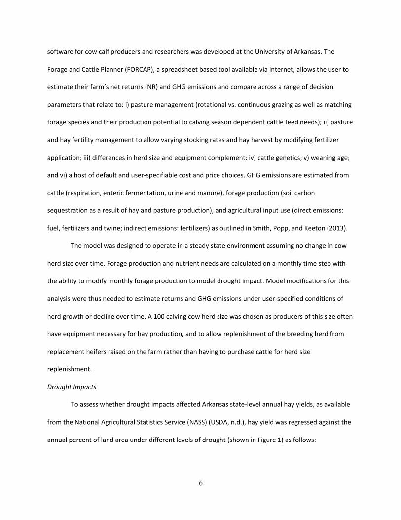
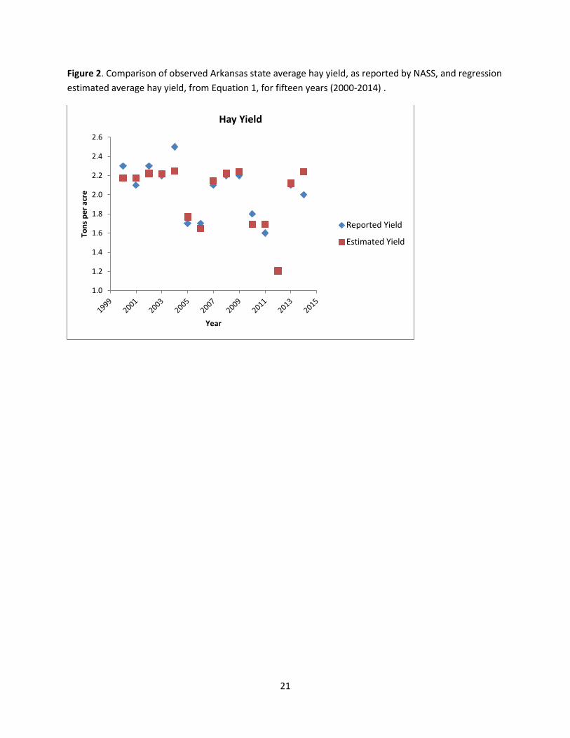
To assess whether drought impacts affected Arkansas state-level annual hay yields, as available

from the National Agricultural Statistics Service (NASS) (USDA, n.d.), hay yield was regressed against the

annual percent of land area under different levels of drought (shown in Figure 1) as follows:

7

(1) Yi = 2.25 - 0.0046 xi0 + 0.0248 xi1 - 0.0716 xi2 + 0.0499 xi3 - 0.1548 xi4 Adj. R2 = 0.82

(0.10)*** (0.0085) (0.0215) (0.0259)** (0.0304) (0.072)*

where Yi is the annual hay yield in year i, xi is percent area in drought in year i and the second subscript

on x is zero through four as per drought levels from Figure 1. Numbers in parentheses on the second line

are standard errors with *, ** and *** indicating level of significance at the 10, 5 and 1% levels,

respectively. Figure 3 depicts actual and estimated hay yield for 2000-2014 and suggested that drought

stress explained a large proportion of the variation in yield in the absence of available data on fertilizer

and hay production practices that might otherwise explain variation in yield.

Therefore, the ratio of estimated yields in Figure 3 to the steady state annual hay yield

assumption in FORCAP of 2.1 ton/acre, to adjust monthly forage production in the model over time, was

deemed a reasonable method to account for drought impact on the yield performance of pastures and

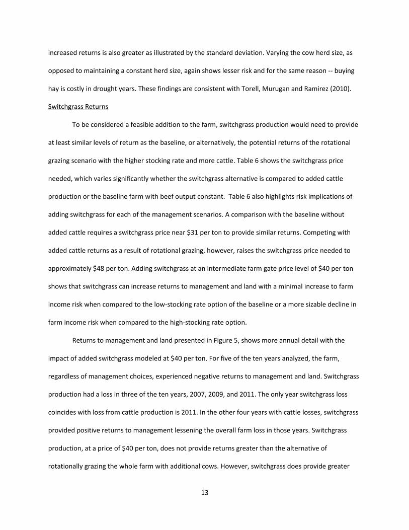
hay land used for cow-calf production. As an example, in a severe drought year, 2011, forage production

in each month as shown in Figure 4 was adjusted downward by 43% to account for risk associated with

droughty conditions. As shown in the bottom two panels of Figure 4, the red bars indicate hay feeding.

While nutrition needs remained constant, pasture forage production to be grazed by animals, needed to

be supplemented to a much larger extent with supplemental hay in a droughty vs. normal year.

To arrive at similar yield implications of drought for Alamo switchgrass, Dr. Rocateli (Rocateli,

2014), a recent Ph.D. graduate at Texas Tech University, was approached to simulate switchgrass yields

from 2004 to 2013 using recent model modifications to ALMANAC, a biophysical crop growth model for

switchgrass initially developed by Kiniry et al. (1996). He used a common soil profile (Captina silt loam)

for pasture conditions in northwest Arkansas along with daily Fayetteville, AR weather data to arrive at

switchgrass yield estimates of a stand that was modeled to be established in 2003.

Using switchgrass cost of production information and methods as shown in Table 1 with a

conservative expectation of a prorated, average yield of 5.01 tons per acre, annual variation in

8

harvesting cost and yields was calculated by adjusting annual yields by the ratio of the annually

estimated ALMANAC yield to the average ALMANAC yield from 2004 to 2013. Table 2 shows annual net

returns to 90 acres of switchgrass as a function of yield and attendant harvest cost fluctuations including

fertilizer price risk, that are summarized as the net future value (NFVS) of earnings due to switchgrass

production as of 2014 as follows:

(2) 𝑁𝐹𝑉𝑆 = ∑ {(𝑝𝑆 ∙ 𝑌𝑆,𝑡 − 𝐶𝑆,𝑡) ∙ (1 + 𝑘)−(𝑡−2014)}2013

𝑡=2004

where pS is the price of switchgrass that would be contractually set with the bio-refinery over the life of

the stand or 10 years, YS,t is the time-varying yield of switchgrass as described above, CS,t are yield- and

fertilizer price-dependent cost of production in constant 2014 dollars as shown in Table 4 and k is the

compounding rate set at 6% p.a.

Modifying the switchgrass price used to arrive at NFVS in Eq. 2, allows estimation of a breakeven

price where the sum of NFVS and the net future value of net returns from cattle and forage production

as calculated annually in FORCAP and summed over time in a similar fashion as shown in Eq. 2 across

different combinations of cattle and switchgrass management practices are the same, or:

(3) 𝑁𝐹𝑉𝑠 + 𝑁𝐹𝑉𝐶𝑎𝑙𝑡= 𝑁𝐹𝑉𝐶𝑏𝑎𝑠𝑒

where 𝑁𝐹𝑉𝐶𝑎𝑙𝑡 is the net future value associated with a cattle management strategy that includes

switchgrass production and 𝑁𝐹𝑉𝐶𝑏𝑎𝑠𝑒 is the net future value of production strategies that do not include

switchgrass production (one option with continuous grazing and a low stocking rate and one option with

rotational grazing and a higher stocking rate).

Cow-calf Baseline Scenario and Alternatives to Compare

Baseline

9

To determine the economic and GHG effects of adding switchgrass production or additional

cattle, to a baseline cattle operation, the following parameters were chosen in FORCAP:

525 acres are divided into 125 hay acres and 400 pasture acres;

Pastures are perimeter fenced with barbed wire with fence corners constructed of steel pipe;

Forage species on pasture land consist of 65 percent fescue, 25 percent bermudagrass and 10

percent clover by area;

Forage species on hay land consist of 40 percent fescue, 50 percent bermudagrass and 10

percent clover by area;

Hay land is fertilized annually with poultry litter applied at two tons per acre and 1 ton per acre

of lime is applied every four years;

Pasture land receives no fertilizer but lime is applied at the same rate as on hay land;

No stockpiling, planting of winter forages, or strip grazing takes place on the farm;

The pastures are continuously grazed;

The cow herd consists of 83 commercial white cows with an average weight of 1,200 pounds

and 17 young cows at a weight of 900 pounds at first calf; 17 replacements are retained and 16

cows are culled each year with a death loss of one cow per year;

The farm maintains four breeding bulls with an average weight of 1,850 pounds – bulls are kept

on farm for four years. One bull is sold and replaced each year;

The farm has calves year round with an average birth weight of 90 pounds and a seven month

average weaning weight for heifers and steers of 520 and 555 pounds respectively;

Replacement heifers are bred at 15 months of age to calve at two years of age;

Fourteen percent breeding failures are expected along with one percent in cow death losses and

three percent in calf death losses each year;

10

The farm feeds hay, forage, and minerals with no supplemental feeding of grains;

Transportation of animals to market consists of one custom hauling trip and five personal

hauling trips each year;

All animals are dewormed once per year. Cows, bulls and replacements are vaccinated with 7-

way Blackleg, 4-way Viral and Vibro-Lepto 5 while calves are vaccinated with 7-way Blackleg and

4-way Viral. Additionally, heifer calves are tested for Brucellosis and bull calves are castrated

and given growth implants. No horns are removed prior to marketing. Pinkeye, scours and

Pasturella are treated on farm on an as needed basis and conditions requiring veterinary visits

include: 2 prolapse, 1 cesarean, 11 sick treatments and 4 bull soundness checks annually;

The buildings on the farm include a 1,000 sqft. Hay barn and an 800sqft. Storage shed;

The farm owns the equipment necessary to bale hay which includes one: 75 hp tractor, disk

mower, hay rake, and round baler;

The farm also owns a stock trailer, hay wagon, brush mower and a corral and chute system;

Default cattle and input prices reflect 2014 conditions with a cattle price option of the past ten-

year deflated average price using overall U.S. beef cattle prices for all cattle and calves.

To establish a baseline scenario, the farm, as described above, required several changes to

model annual variation and included: i) changing hay yield in Figure 3 and hay prices as shown in Table

3; ii) changing cattle prices as shown in Table 3; iii) model runs with a static cow herd, where the farm

balances the sale of cull cows and replacement heifers each year to maintain 100 cows; and iv) model

runs with a fluctuating cow herd where the herd increases, by retaining more heifer calves, and

decreases, by selling more cull cows, in a similar pattern as that recorded for the Arkansas state cow

herd numbers for the period of 2004 – 2013 as shown in Table 4. The move from a static to a varying

cow herd size over time is expected to capture the effect of drought on herd size as well as producer

responses to changing cattle and input costs. The results of these model runs are thus expected to show

11

net returns and GHG emissions that result as a function of varying hay yields and prices, mainly due to

climatic conditions and either constant or changing beef output at varying cattle prices. The baseline

scenario thus utilizes 400 pasture acres using continuous grazing with attendant performance statistics

using either a static or fluctuating herd size.

Rotational Grazing Impact and Management Alternatives to Baseline

When changing from a continuous grazing strategy to a rotational grazing strategy, the baseline

model farm increases grazing efficiency, the ratio of grazed forage intake as a fraction of total animal

feed needs, from 46% to 56% as rotational grazing allows the operator to rest pastures and minimize

forage losses as a result of selective grazing (Teague, Dowhower, and Waggoner, 2004). The main effect

is that holding stocking rate, or beef output, constant, the operation is now able to free 90 acres of

pasture for alternative use. Investment in extra fencing is required, but now on fewer acres with a net

investment increase of less than $1,000 and modeled using default parameters in FORCAP. Importantly,

hay feeding needs change only marginally, with the need for purchased hay increasing from 198 bales

under continuous grazing to 207 bales under rotational grazing under normal forage production

conditions. It is these 90 pasture acres that are now available for switchgrass production as the first

alternative to the baseline with the alternative now grazing 100 cows on 310 acres of pasture.

A second alternative holds the 400 acres of pasture constant, also changes to rotational grazing

requiring an additional approximate $6,000 in fencing investment and increasing the herd size to 113

calving cows thereby increasing beef output while not significantly modifying hay imports to the farm

(now at 195 bales vs. 198 bales with continuous grazing).

These alternatives thus represent a more intensive use of pasture land by either diversifying to

switchgrass production and a greater cattle stocking rate or more cattle at the same greater stocking

rate. Implications of climatic variation are captured in net returns to cattle and switchgrass production

(if any) under either constant beef output over time or fluctuating beef output. Price risk in constant

12

2014 dollars includes fertilizer, hay and cattle price risk as these represent the main cost categories for

the enterprises analyzed. Production risk is captured by variations in hay and pasture yields as described

above as well as simulated switchgrass yield risk.

RESULTS

Cow-calf Return Comparisons

Table 5 shows the farms’ cash returns, returns to management and land, total CO2 equivalent

emissions (GHG emissions – GHG sequestration), hay bought or sold and days on feed for the baseline

and alternative production strategies for the static and fluctuating herd sizes, respectively. The

switchgrass enterprise was not added to the middle column, the scenario where the pasture area was

reduced to free up acreage for switchgrass (Rotational 310), to highlight impacts of cattle enterprise

changes without the influence of switchgrass. Table 5 suggests that varying the cow herd size over time

increased average annual returns and decreased average days on feed, hay purchased, and CO2

equivalent emissions compared to a static herd size. Varying the herd numbers also decreased the

standard deviation of returns such that cash flows from herd liquidation and rebuilding tended to lessen

financial risk when compared to maintaining a static herd size by buying needed hay or selling excess

hay. The farm, prior to any management changes, has average cash returns of $16,934 and $19,247

when their herd number is static and varying, respectively. Varying the herd is especially beneficial in

drought years as a means to mitigate cash return losses by reducing hay requirements for the herd. This

is reflected in the minimum cash return of -$13,568 for varying the herd compared to -$24,954 for a

static herd in 2012 (not shown in Table 5) in the only year in which cash returns for all cattle scenarios,

prior to the switchgrass addition, was negative.

Both rotational grazing strategies, under both static and varying cow herd numbers, prior to

assessing switchgrass production returns, increase farm returns, however, the risk associated with the

13

increased returns is also greater as illustrated by the standard deviation. Varying the cow herd size, as

opposed to maintaining a constant herd size, again shows lesser risk and for the same reason -- buying

hay is costly in drought years. These findings are consistent with Torell, Murugan and Ramirez (2010).

Switchgrass Returns

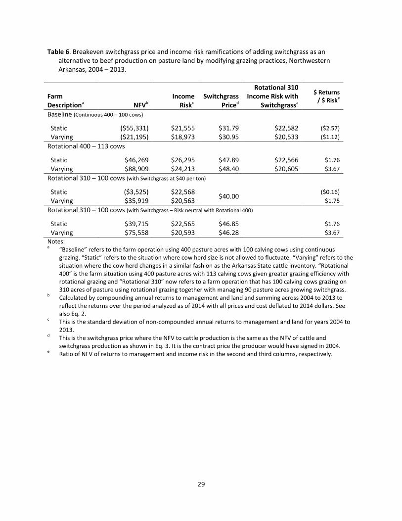
To be considered a feasible addition to the farm, switchgrass production would need to provide

at least similar levels of return as the baseline, or alternatively, the potential returns of the rotational

grazing scenario with the higher stocking rate and more cattle. Table 6 shows the switchgrass price

needed, which varies significantly whether the switchgrass alternative is compared to added cattle

production or the baseline farm with beef output constant. Table 6 also highlights risk implications of

adding switchgrass for each of the management scenarios. A comparison with the baseline without

added cattle requires a switchgrass price near $31 per ton to provide similar returns. Competing with

added cattle returns as a result of rotational grazing, however, raises the switchgrass price needed to

approximately $48 per ton. Adding switchgrass at an intermediate farm gate price level of $40 per ton

shows that switchgrass can increase returns to management and land with a minimal increase to farm

income risk when compared to the low-stocking rate option of the baseline or a more sizable decline in

farm income risk when compared to the high-stocking rate option.

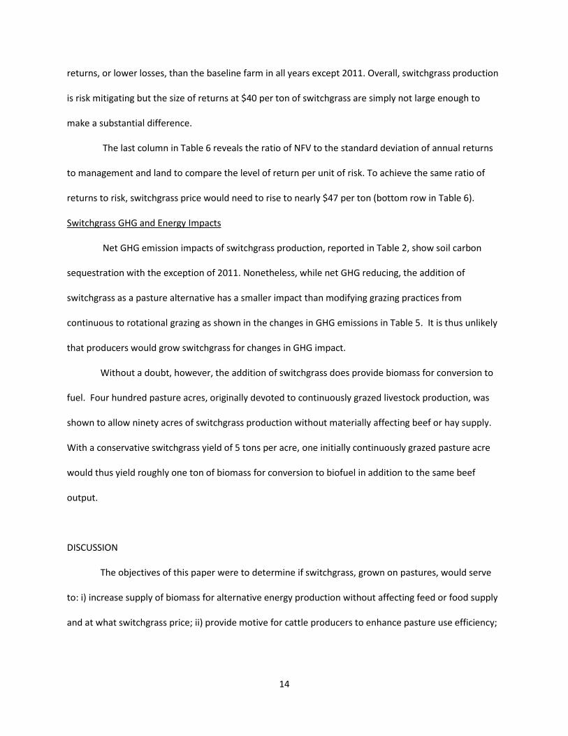
Returns to management and land presented in Figure 5, shows more annual detail with the

impact of added switchgrass modeled at $40 per ton. For five of the ten years analyzed, the farm,

regardless of management choices, experienced negative returns to management and land. Switchgrass

production had a loss in three of the ten years, 2007, 2009, and 2011. The only year switchgrass loss

coincides with loss from cattle production is 2011. In the other four years with cattle losses, switchgrass

provided positive returns to management lessening the overall farm loss in those years. Switchgrass

production, at a price of $40 per ton, does not provide returns greater than the alternative of

rotationally grazing the whole farm with additional cows. However, switchgrass does provide greater

14

returns, or lower losses, than the baseline farm in all years except 2011. Overall, switchgrass production

is risk mitigating but the size of returns at $40 per ton of switchgrass are simply not large enough to

make a substantial difference.

The last column in Table 6 reveals the ratio of NFV to the standard deviation of annual returns

to management and land to compare the level of return per unit of risk. To achieve the same ratio of

returns to risk, switchgrass price would need to rise to nearly $47 per ton (bottom row in Table 6).

Switchgrass GHG and Energy Impacts

Net GHG emission impacts of switchgrass production, reported in Table 2, show soil carbon

sequestration with the exception of 2011. Nonetheless, while net GHG reducing, the addition of

switchgrass as a pasture alternative has a smaller impact than modifying grazing practices from

continuous to rotational grazing as shown in the changes in GHG emissions in Table 5. It is thus unlikely

that producers would grow switchgrass for changes in GHG impact.

Without a doubt, however, the addition of switchgrass does provide biomass for conversion to

fuel. Four hundred pasture acres, originally devoted to continuously grazed livestock production, was

shown to allow ninety acres of switchgrass production without materially affecting beef or hay supply.

With a conservative switchgrass yield of 5 tons per acre, one initially continuously grazed pasture acre

would thus yield roughly one ton of biomass for conversion to biofuel in addition to the same beef

output.

DISCUSSION

The objectives of this paper were to determine if switchgrass, grown on pastures, would serve

to: i) increase supply of biomass for alternative energy production without affecting feed or food supply

and at what switchgrass price; ii) provide motive for cattle producers to enhance pasture use efficiency;

15

and iii) quantify, and potentially reduce, income variability with switchgrass as an income stabilizing

enterprise under droughty conditions.

Biofuel refineries seeking land devoted to bioenergy crops in a proximal radius of the plant, to

limit transportation costs, will need to secure this land through long term contracts or leases (Mohua et

al. 2014). Given this need to source cellulosic material close to the plant, pasture land will come under

scrutiny as a source for biomass. This study offers an analysis of economic and environmental tradeoffs

associated with the practice of rotational grazing and higher cattle stocking rate. It shows under what

switchgrass price conditions, pasture land may be converted to dedicated energy crop production.

Switchgrass is shown to have income risk mitigating effects under droughty conditions. However, to

compete with an alternative of added cattle production, switchgrass prices approach nearly $50 per ton

to compete given the cattle producer conditions evaluated in this analysis. At the same time, positive

environmental impacts associated with adding switchgrass production were found to be minor at a

conservative yield estimate of 5 tons per acre (ALMANAC yields were 7.85 tons per acre per year, for

example).

Limitations to this study are that only one farm size and operation type was studied. It may well

be that operation size could have larger implications than provided here. Baling an annual average of

450 tons of switchgrass using an 800lb bale size, for example, may soon have the operator looking to

larger haying equipment given the number of bales produced. By the same token, other pasture

alternatives may include other forms of grazing livestock. Drought years may also lead to the release of

Conservation Reserve Program (CRP) acreage for grazing or haying and hence hay yield risk may not be

as severe as modeled within. Finally, cow herd size changes for the average of a state is likely an

underestimate of the types of changes that would occur from farm to farm and hence the income risk of

cattle production may be low in the varying herd size scenarios. The breakeven prices for switchgrass in

Table 6 are thus offered as a way to show a possible range of price levels that are a function of a number

16

of factors that will drive beef producer willingness to accept offers to produce switchgrass. It is clear

that GHG implications will likely play a minor role although higher switchgrass yields are certainly in the

realm of possibilities and would heighten the potential for soil carbon sequestration as modeled here.

17

References

Barney, J., J. Mann, G. Kyser, E. Blumwald, A. Van Deynze, and J. DiTomaso. 2009. Tolerance of switchgrass to extreme soil moisture stress: Ecological implications. Plant Science 177(6): 724–732.

Bonner, I., K. Cafferty, D. Muth, M. Tomer, D. James, S. Porter, and D. Karlen. 2014. Opportunities for Energy Crop Production Based on Subfield Scale Distribution of Profitability. Energies 7(10): 6509–6526.

Debnath, D., A. Stoecker, and F. Epplin. 2014. Impact of environmental values on the breakeven price of switchgrass. Biomass and Bioenergy 70: 184–195.

Doye, D., M. Popp, and C. West. 2008. Controlled vs. continuous calving seasons in the South: What’s at stake? Journal of the American Society of Farm Managers and Rural Appraisers 71(1): 60-73.

Frank, A., J. Berdahl, J. Hanson, M. Liebig and H. Johnson. 2004. Biomass and Carbon Partitioning in Switchgrass. Crop Science 44: 1391-1396.

Girouard, P., C. Zan, B. Mehdi, and R. Samson. 1999. Economics and Carbon Offset Potential of Biomass Fuels. Resource Efficient Agricultural Production (REAP) – Canada.

Gouzaye, A., F. Epplin, Y. Wu, and S. Makaju. 2014. Yield and Nutrient Concentration Response to Switchgrass Biomass Harvest Date. Agronomy Journal 106: 793–99.

Jennings, J., and S. Jones, n.d.. DIVISION OF AGRICULTURE Arkansas 300 Days Grazing System – Getting

Started.

Kells, B. J., and S. Swinton. 2014. Profitability of cellulosic biomass production in the northern great lakes region. Agronomy Journal 106(2): 397–406.

Kiniry, J., M. Sanderson, J. Williams, C. Tischler, M. Hussey, W. Ocumpaugh, J. Read, G. VanEsbroeck and R. Reed. 1996. Simulating Alamo switchgrass with the ALMANAC model. Agronomy Journal 88: 602-606.

Lal, R. 2004. Carbon emission from farm operations. Environment International, 30(7): 981-990.

Lee, D., V. Owens, J. Doolittle. 2007. Switchgrass and Soil Carbon Sequestration Response to Ammonium Nitrate, Manure, and Harvest Frequency on Conservation Reserve Program Land. Agronomy Journal 99: 462-468.

Lemus, R., C. Brummer, K. Moore, N. Molstad, L. Burras and M. Barker. 2002. Biomass Yield and Quality of 20 Switchgrass Populations in Southern Iowa, USA. Biomass & Bioenergy 23(6): 433-442.

Ma, Z., C. Wood, and D. Bransby. 2000a. Carbon dynamics subsequent to establishment of switchgrass. Biomass and Bioenergy 18(2): 93–104.

Ma, Z., C. Wood, and D. Bransby. 2000b. Soil Management impacts on soil carbon sequestration by switchgrass. Biomass and Bioenergy 18: 469-477.

18

McLaughlin, S. B., and L. Kszos. 2005. Development of switchgrass (Panicum virgatum) as a bioenergy feedstock in the United States. Biomass and Bioenergy 28(6): 515–535.

Mohua, H, F. Epplin, J. Biermacher, R. Holcomb, P. Kenkel. 2014. Marginal cost of delivering switchgrass feedstock and producing cellulosic ethanol at multiple bio-refineries. Biomass and Bioenergy 66: 308-319

Monti, A., L. Barbanti, A. Zatta, and W. Zegada-Lizarazu. 2012. The contribution of switchgrass in reducing GHG emissions. GCB Bioenergy 4(4): 420–434.

National Drought Mitigation Center (NDMC). n.d. United States Drought Monitor- Tabular Data Archive. Accessed 5-2015.

Popp, M., and R. Hogan Jr. 2007. Assessment of Two Alternative Switchgrass Harvest and Transport Methods. In Farm Foundation Conference Paper. St. Louis, MO.

Popp, M., L. Nalley, C. Fortin, A. Smith and K. Brye. 2011. Estimating Net Carbon Emissions and Agricultural Response to Potential Carbon Offset Policies. Agronomy Journal 103: 1132-1143.

Popp, M., S. Searcy, S. Sokhansanj, J. Smartt, and N. Cahill. 2015. Influence of weather on the predicted moisture content of field chopped energy sorghum and switchgrass. Applied Engineering in Agriculture 31(2): 179-190.

Qualls, D. J., K. Jensen, C. Clark, B. English, J. Larson, and S. Yen. 2012. Analysis of factors affecting willingness to produce switchgrass in the southeastern United States. Biomass and Bioenergy 39: 159–167.

Raneses, A., H. Kenneth, and H. Shapouri. 1998. Economic impacts from shifting cropland use from food to fuel. Biomass and Bioenergy 15(6): 417–422.

Rocateli, A. 2014. Enhancing ALMANAC for simulating Switchgrass Biomass Production and Macronutrient Removal. Unpublished Ph.D. Dissertation. Texas Tech Univeristy, Lubbock, TX.

Sharp, B. E., and S. Miller. 2014. Estimating maximum land use change potential from a regional biofuel

industry. Energy Policy 65: 261–269.

Smith, A., M. Popp, and D. Keeton. 2013. Forage and Cattle Planner ( FORCAP ) Reference Manual, 2013.

Stroup, J. A., M. Sanderson, J. Muir, M. McFarland, and R. Reed. 2003. Comparison of growth and performance in upland and lowland switchgrass types to water and nitrogen stress. Bioresource Technology 86(1): 65–72.

Teague, W., S. Dowhower, and J. Waggoner. 2004. Drought and grazing patch dynamics under different grazing management. Journal of Arid Environments 58(1): 97-117.

Torell, L. A., S. Murugan, and O. Ramirez. 2010. Economics of Flexible Versus Conservative Stocking Strategies to Manage Climate Variability Risk. Rangeland Ecology & Management 63(4): 415–425.

United States Department of Agriculture (USDA). n.d. National Agricultural Statistics Service-Quick Stats. Accessed 5-2015.

19

Vadas, P. a., K. Barnett, and D. Undersander. 2008. Economics and Energy of Ethanol Production from Alfalfa, Corn, and Switchgrass in the Upper Midwest, USA. BioEnergy Research 1: 44-55.

Walsh, M. E., D. De La Torre Ugarte, H. Shapouri, and S. Slinsky. 2003. Bioenergy crop production in the United States: Potential quantities, land use changes, and economic impacts on the agricultural sector. Environmental and Resource Economics 24(4): 313–333.

Wang, T., S. Park, S. Bevers, R. Teague, and J. Cho. 2013. Factors affecting cow-calf herd performance and greenhouse gas emissions. Journal of Agricultural and Resource Economics 38(3): 435–456.

West, C. 2015. Thornton Distinguished Chair in Forage Systems. Personal Communication.

Zilverberg, C. J., P. Johnson, J. Weinheimer, and V. Allen, 2011. Energy and Carbon Costs of Selected Cow-Calf Systems. Rangeland Ecology & Management 64(6): 573–584.

20

Figure 1. The annual average percent area of the state of Arkansas in each drought category (D0-D4) as

reported by USDM.

Figure 2. The annual number of weeks in each drought category (D1-D4) per year in the state of

Arkansas as reported by USDM.

0

10

20

30

40

50

60

70

80

90

100

Pe

rce

nt

Are

a

Year

Area in Drought

D4

D3

D2

D1

D0

0

4

8

12

16

20

24

28

32

36

40

44

48

52

We

eks

Year

Weeks in Drought

D4

D3

D2

D1

21

Figure 2. Comparison of observed Arkansas state average hay yield, as reported by NASS, and regression

estimated average hay yield, from Equation 1, for fifteen years (2000-2014) .

1.0

1.2

1.4

1.6

1.8

2.0

2.2

2.4

2.6

Ton

s p

er

acre

Year

Hay Yield

Reported Yield

Estimated Yield

22

Bench / Your Farm

Hay Land Grazing

Species -- Default Jan Feb Mar Apr May Jun Jul Aug Sep Oct Nov Dec Total

Bermuda 0% 0% 0% 0% 10% 25% 35% 20% 10% 0% 0% 0% 100%

Fescue 0% 3% 7% 20% 27% 15% 0% 0% 2% 13% 11% 2% 100%

Orchardgrass 0% 0% 15% 25% 25% 10% 3% 2% 5% 10% 5% 0% 100%

Clovers 0% 0% 5% 20% 25% 20% 5% 0% 5% 15% 5% 0% 100%

Available Forage vs. Grazing Intake (incl. Extra Cattle if any)

Monthly Forage Available By Species (Your Farm)

OK

OK

OK

OK

Bench / Your Farm

Hay Land Grazing

Species -- Default Jan Feb Mar Apr May Jun Jul Aug Sep Oct Nov Dec Total

Bermuda 6% 14% 20% 11% 6% 57%

Fescue 2% 4% 11% 15% 9% 0% 0% 1% 7% 6% 1% 57%

Orchardgrass 0% 0% 9% 14% 14% 6% 2% 1% 3% 6% 3% 0% 57%

Clovers 3% 11% 14% 11% 3% 0% 3% 9% 3% 57%

Available Forage vs. Grazing Intake (incl. Extra Cattle if any)

Monthly Forage Available By Species (Your Farm)

OK

OK

OK

OK

Figure 4. Example of Forage Production adjustment and resultant change in hay needs as a result of

drought. Top panel is the base year seasonal distribution of forage production. The middle panel reflects

a 43% reduction in forage production. The bottom left panel shows the forage balance corresponding

with a normal production year and the bottom right panel shows increasing reliance on hay (the red

portion of the bar) under severe drought. While Orchardgrass growth is listed in the figure below it was

not planted on any acres and thus has no effect on forage balance.

Normal Drought

Normal

Drought

23

Figure 5. Comparison of Annual Net Returns to Management and Labor with a Static or Varying Cow

Herd Size, Modified Stocking rate with Rotational Grazing and Diversification with Switchgrass at $40 per

ton.

-$60

-$40

-$20

$0

$20

$40

$60

2004 2005 2006 2007 2008 2009 2010 2011 2012 2013

Tho

usa

nd

s

Static Herd Size

Baseline - Static Rotational 400 - Static Rotational 310 - Static Switchgrass

-$40

-$20

$0

$20

$40

$60

2004 2005 2006 2007 2008 2009 2010 2011 2012 2013

Tho

usa

nd

s

Varying Herd Size

Baseline - Varying Rotational 400 - Varying Rotational 310 - Varying Switchgrass

24

Table 1. Baled Switchgrass Stored at Field Side including Storage and Grinding Losses. Estimated Cost of

Production on Pasture Land, Arkansas, 2014.a

Description Total Cost ($) Prorated Present Value of Total Cost Over Useful Life of Stand at 6% ($)

Establishment Year Pre-Plant Weed Control

b 25.00 2.50

Field Preparation c

137.34 13.73 Planting

d 96.67 9.67

Post-Plant Weed Control e 38.90 3.89

Operating Interest f 22.58 2.26

Total Specified Expenses 320.48 Replant Charge

g 80.12 8.01

Year 2 Fertilizer

h 111.51 10.51

Harvest i

53.56 5.05

Operating Interest j 5.76 0.54

Total Specified Expenses 167.60

Years 3+ Fertilizer

h 111.51 65.33

Harvest i

74.13 43.43 Operating Interest

j 6.32 3.70

Total Specified Expenses

191.96

Total Specified Expenses - PV over useful Life k $168.63

Useful Life of Stand 10 yrs Dry Matter Yield - Year 2 4.5 tons Dry Matter Yield - Year 3+ 6.25 tons Prorated Dry Matter Yield - Net of Losses 5.01 tons/acre Breakeven Price per dry ton

l $44.86

Prorated Annual GHG emissions in lbs of CO2 per acre

m 896

Annual Soil Carbon Sequestration in lbs of CO2 per acre n

1,034 Notes: a Please contact authors for further cost of production details not included below. All fertilizer and herbicide are custom applications at $6/acre. Cost information

is the deflated ten year average for fertilizers. Switchgrass seed is $10/lb of pure live seed and diesel fuel is $3.17/gal. Operating interest and the capital recovery rate are charged at 7.75% and 6%, respectively. Operator and hired labor are charged at $9.25 and $8.00/hr, respectively.

b This includes 2 lb a.i. or 4 pt of glyphosate (Roundup) at $4.75 per pt in late March to kill existing vegetation. c Field preparation occurs in April and includes two passes with a disk to break sod and incorporate 1 ton of lime, 55 lbs of phosphate (0-45-0) and 120 lbs of

potash (0-0-60) fertilizers. One pass with a cultipacker smoothes the field. Fertilizers are custom applied. d A no-till grass seed planter is rented at $150 per day in early May. Seeding rate is 8 lbs of pure live seed at $10 per pound. e Herbicide application of 0.33 lb a.i. quinclorac (Paramount) at $55 per lb a.i. and 0.5 oz a.i. imazapyr (Ally or Cimaron) at $29.50 per oz a.i. f Operating interest is charged on all expenses except capital recovery on owned equipment for 1 year given the lack of harvest in the establishment year. g Replanting charges include the fraction of total specified expenses for the establishment year that did not establish (25%).

h The fertilizer program is the same as the establishment year with the addition of 200 lbs of ammonium nitrate (34-0-0) for year 2 and onward and no more lime.

Nutrient replacement is not scaled for yield differences between years 2 and 3+. i Harvest is performed using a mower conditioner, hay rake (25% of acreage), small round baler (#680 dry matter or #800 as is 15% moisture) using twine and an

automatic bale mover for staging without tarp or storage pad preparation. Costs increase with yield beyond year 2. j Operating interest is again applied to operating expense except for only half year given sale of product. k This represents the average, discounted per acre annual cost adjusted for yield and cost differences across the life of the stand at establishment.

l This is the breakeven price at establishment adjusted for timing of yield which is adjusted for baling, storage and transport losses of 8%. m

Greenhouse gas emissions include diesel fuel use emissions, direct and indirect fertilizer emissions as well as emissions from use of chemicals and twine using values of Lal, et al. (2004).

n Carbon sequestration is a function of the shoot:root ratio of 2.05 (Ma et al., 2000b; Lee et al., 2007), 42% carbon content in above and below ground biomass (Lemus et al., 2002; Girouard et el., 1999; Frank et al., 2004) and a 10% of above ground harvested biomass remaining as stubble and crown. Carbon sequestered is thus a function of yield as 50% of the carbon in decomposing root biomass is expected to remain in the soil. Given the perennial growth habit, however, only 1/3rd of the root system dies off each year (West, 2015). Finally, it is expected that 5% of the non-harvested above ground biomass comes in soil contact via equipment traffic and thereby available for soil carbon sequestration with soil carbon fluxes affected by soil texture as in Popp et al. (2011). The switchgrass growth model ALMANAC (Kiniry et al., 1996) recently updated by Rocateli (2014) uses a Captina silt loam which to a depth of 55 cm is classified as 31% sandy, 32% loamy and 37% clayey. This leads to approx. 72% of captured carbon remaining in the soil long term.

25

Table 2. Fertilizer price, yield, harvest cost, operating interest, GHG impacts and Returns to Alamo Switchgrass production on 90 acres, Captina Silt Loam soils, Fayetteville, AR, 2004 to 2013 using yield estimates generated by ALMANAC and adjusted to 5.01 tons/acre at a switchgrass price of $40 per dry ton as stored at the side of the field in 800 lb round bales.

Notes: a Net returns to management and land include all costs shown in Table 1 with the exception of varying fertilizer and yield-dependent harvest costs and

exclude labor charges on the 90 acres of pasture modeled. b Net future value is the sum of annual net returns compounded to 2014 as shown in Eq. 2 at 6%.

c Standard deviation of annual net returns.

d Based on the 90 acres of switchgrass with fuel use, fertilizer direct and indirect emissions as well as emissions for twine and chemicals. Emissions include

farm activities to the point of staging bales at the side of the field and do not include transport emissions to the bio-refinery.

Production Year 2004 2005 2006 2007 2008 2009 2010 2011 2012 2013

Fertilizer in 2014 dollars Phosphate $/ton 594 574 587 608 645 730 632 607 693 694

Potash $/ton 404 470 495 407 452 975 637 577 632 589

Ammonium Nitrate $/ton 587 560 663 555 410 501 496 460 546 539

Lime $/ton 47.10 40.50 37.50 32.41 18.55 31.31 34.29 44.53 54.66 54.36

Fertilizer Cost $/acre $104.71 $105.09 $115.84 $100.94 $90.29 $133.36 $110.31 $103.74 $118.16 $114.94

Yield dry ton/acre 5.39 5.62 5.28 4.37 4.63 4.48 5.02 3.75 5.59 5.97

Harvest cost $/acre $52.69 $54.46 $52.39 $46.85 $48.41 $47.55 $50.83 $43.05 $54.29 $56.60

Operating interest $/acre $5.34 $5.40 $5.74 $4.95 $4.60 $6.23 $5.46 $4.91 $5.90 $5.87

Annual Net Returns to Management and Land in 2014 dollars (excluding labor)

a $/farm $2,378 $2,997 $960 ($399) $1,371 ($3,086) $703 ($2,553) $1,689 $3,142

GHG emissions (CO2 eq. lb/acre) 910 918 905 873 882 877 896 850 917 931 GHG sequestration (CO2 eq. lb/acre) 1112 1159 1089 901 954 925 1036 773 1153 1231 net GHG sequestration (CO2 eq. lb/acre) 203 241 183 29 72 48 140 (77) 236 301

NFVS b

$11,141 Standard Deviation c

$2,152

Average and Standard Deviation of tons of GHG Sequestered

d 6.2 (5.3)

26

Table 3. Annual hay and cattle price in 2014 dollars.

Production Year 2004 2005 2006 2007 2008 2009 2010 2011 2012 2013

Hay Pricea $/bale 39.19 56.62 70.25 62.73 46.53 41.51 46.00 46.46 52.80 49.90

Cattle Type Prices $/cwt

Steersb, c

4-500 lb. 214.70 220.04 228.19 208.47 197.41 206.81 205.50 202.95 221.56 217.55

5-600 lb. 196.75 199.78 206.61 192.75 182.91 191.09 191.57 189.39 201.54 196.10

6-700 lb. 182.17 188.29 189.52 179.82 170.90 177.99 179.44 177.24 184.69 180.32

7-800 lb. 171.01 178.25 176.37 169.51 161.81 168.64 169.41 168.45 173.74 169.92

Heifersb,

c

4-500 lb. 195.15 203.56 202.78 182.28 170.67 175.89 178.40 177.69 192.97 191.07

5-600 lb. 181.70 189.02 187.23 171.23 162.28 167.44 169.13 168.24 179.30 175.89

6-700 lb. 170.63 176.20 175.23 163.42 155.45 161.52 162.27 160.46 168.14 165.04

7-800 lb. 160.74 166.64 165.25 156.61 149.88 155.28 156.60 153.79 158.01 156.19

Cowsb, d 75-80% Lean 86.44 86.50 80.67 80.37 83.73 82.90 88.10 90.69 95.42 93.45

Bullsb, e 1-2,000 lb. 110.01 108.80 99.52 100.26 105.39 104.84 106.83 107.11 112.86 114.67 Notes: a Reported by USDA, NASS as $/ton, converted to $/800lb bale and adjusted for inflation to constant 2014 dollars.

b State average market prices as reported by the USDA, Agricultural Marketing Service. Yearly average prices of all monthly prices are weighted by

15,18,14,9,5,5,3,3,8,8,8,4 percent for January through December, respectively as in Doye et al. (2008). All prices are reported in $/cwt and are deflated to 2014 using the beef cattle price deflator option in FORCAP.

c Medium and large frame No. 1

d Breaking Utility and Commercial

e Yield grade 1-2

27

Table 4. Annual change in the number of calving cows, consistent with recorded changes in the Jan. 1, Arkansas state cow herd inventory numbers, for both rotationally grazing 310 acres with 100 cows and 400 acres with 113 cows.

Rotationally Grazing 310 acres with 100 cows

Production Year 2004 2005 2006 2007 2008 2009 2010 2011 2012 2013

Total Cows ab

104 102 95 97 99 95 98 97 96 89

Old Cows 84 85 78 78 81 79 79 81 80 73

Young Cows 20 17 17 19 18 16 19 16 16 16

Replacements c 17 17 19 18 16 19 16 16 16 16

Cull Cows d 18 23 16 15 19 15 16 16 22 14

Death Loss 1 1 1 1 1 1 1 1 1 1

Rotationally Grazing 400 acres with 113 cows

Total Cows ab

118 115 107 110 112 107 111 110 108 100

Old Cows 95 96 88 89 92 88 89 92 90 82

Young Cows 23 19 19 21 20 19 22 18 18 18

Replacements c 19 19 21 20 19 22 18 18 18 18

Cull Cows d 21 26 17 17 23 17 18 19 25 16

Death Loss 1 1 1 1 1 1 1 1 1 1

Notes: a Adjusted annual herd numbers based on the annual change in Arkansas state cow herd numbers as reported

by NASS. b Began accounting for herd change in 2000 with 100 and 113 cows for Rotational 310 and Rotational 400

respectively. Replacement heifers from the previous year are the young cows of the current year. Old cows are culled, death losses are assumed to occur in the old cow category and young cows from the previous year are added to the inventory of old cows defined as those that have had 2 or more calves.

c Increased in years with herd growth.

d Increased in years with herd decline.

28

Table 5. Cattle Performance Statistic Summary for Static and Varying Herdsizes from 2004 to 2013 in

Arkansas. Economic Data is expressed in 2014 dollars.

Static Cow Numbers Baseline a Rotational 310 b Rotational 400 c

Average St. Dev. Average St. Dev. Average St. Dev.

No. of Cows 100 - 100 - 113 -

Pasture Forage Growth d 2,635 1,089 2,635 1,089 2,635 1,089

Estimated Days on Feed 203 56 211 55 197 57

Hay Sold/(Bought) e (390) 420 (402) 441 (433) 521

Gross Income f $84,351 $4,214 $84,382 $4,286 $97,307 $5,515

Cash Returns g $16,934 $21,555 $20,185 $22,488 $25,678 $26,295

Returns to Management and Land

h

($5,035) $21,555 ($2,099) $22,488 $2,009 $26,295

Total CO2 Equivalent i 491 27 488 26 542 31

NFV i ($55,331)

($14,666)

$46,269

Varying Cow Numbers k

No. of Cows 97.2 4 97.2 4 109.8 5

Pasture Forage Growth d 2,635 1,089 2,635 1,089 2,635 1,089

Estimated Days on Feed 200 56 207 56 194 56

Hay Sold/(Bought) e (345) 393 (353) 418 (359) 505

Gross Income f $84,005 $8,263 $83,977 $8,214 $96,501 $9,557

Cash Returns g $19,247 $19,073 $22,949 $20,321 $28,549 $24,305

Returns to Management and Land

h

($2,569) $18,973 $818 $20,237 $5,087 $24,213

Total CO2 Equivalent i 477 27 474 26 524 31

NFV j ($21,195) $24,778 $88,909

Notes: a Continuous grazing on 400 pasture acres with 100 cows.

b Rotational grazing on 310 pasture acres with 100 cows to set aside 90 acres for switchgrass. Switchgrass

returns are not included. c Rotational grazing on 400 acres with 113 cows.

d in pounds of available forage/acre per year.

e 800lbs per bale as is weight.

f Income from sale of caves, cull cows and bulls as well as excess bales of hay if any.

g Gross income less direct costs of feed, fertilizer, veterinary and drug, minerals, marketing and hauling, fuel,

repair and maintenance and operating interest (charged at ½ total direct costs). h Cash returns less ownership charges (capital recovery, opportunity cost on breeding stock, property tax and

insurance). Fixed costs are constant across years in the static herd but vary with cow numbers as the opportunity cost of breeding stock changes.

i Net carbon emissions from cattle (respiration, enteric fermentation, and nitrous oxide), soil carbon

sequestration by forages and hay, and agricultural inputs (fertilizer – CO2and NO2, fuel and other) as reported by FORCAP and expressed in tons per farm.

j Net Future Value of net returns to management and land calculated using Eq. 2.

k Adjusted annual herd numbers based on the annual change in Arkansas state cow herd numbers as reported

by NASS and shown in Table 6.

29

Table 6. Breakeven switchgrass price and income risk ramifications of adding switchgrass as an alternative to beef production on pasture land by modifying grazing practices, Northwestern Arkansas, 2004 – 2013.

Farm Descriptiona NFVb

Income Riskc

Switchgrass Priced

Rotational 310 Income Risk with

Switchgrassa

$ Returns / $ Risk

e

Baseline (Continuous 400 – 100 cows)

Static ($55,331) $21,555 $31.79 $22,582 ($2.57) Varying ($21,195) $18,973 $30.95 $20,533 ($1.12)

Rotational 400 – 113 cows

Static $46,269 $26,295 $47.89 $22,566 $1.76 Varying $88,909 $24,213 $48.40 $20,605 $3.67

Rotational 310 – 100 cows (with Switchgrass at $40 per ton)

Static ($3,525) $22,568 $40.00

($0.16) Varying $35,919 $20,563 $1.75

Rotational 310 – 100 cows (with Switchgrass – Risk neutral with Rotational 400)

Static $39,715 $22,565 $46.85 $1.76

Varying $75,558 $20,593 $46.28 $3.67

Notes: a

“Baseline” refers to the farm operation using 400 pasture acres with 100 calving cows using continuous grazing. “Static” refers to the situation where cow herd size is not allowed to fluctuate. “Varying” refers to the situation where the cow herd changes in a similar fashion as the Arkansas State cattle inventory. “Rotational 400” is the farm situation using 400 pasture acres with 113 calving cows given greater grazing efficiency with rotational grazing and “Rotational 310” now refers to a farm operation that has 100 calving cows grazing on 310 acres of pasture using rotational grazing together with managing 90 pasture acres growing switchgrass.

b Calculated by compounding annual returns to management and land and summing across 2004 to 2013 to reflect the returns over the period analyzed as of 2014 with all prices and cost deflated to 2014 dollars. See also Eq. 2.

c This is the standard deviation of non-compounded annual returns to management and land for years 2004 to

2013. d This is the switchgrass price where the NFV to cattle production is the same as the NFV of cattle and

switchgrass production as shown in Eq. 3. It is the contract price the producer would have signed in 2004. e

Ratio of NFV of returns to management and income risk in the second and third columns, respectively.