Embed Size (px)
Citation preview
THE IMPACT OF SWITCHGRASS PRODUCTION ON
OKLAHOMA HAY MARKETS
By
KWAME ACHEAMPONG
Bachelor of Science Agriculture
University of Cape Coast
Cape Coast, Ghana
2005
Submitted to the Faculty of the Graduate College of the
Oklahoma State University In partial fulfillment of
the requirements for the Degree of
MASTER OF SCIENCE December 2009
ii
THE IMPACT OF SWITCHGRASS PRODUCTIO ON
OKLAHOMA HAY MARKETS
Thesis Approved:
Dr Brian D. Adam
Thesis Adviser
Dr Michael R. Dicks
Dr. Jody L. Campiche
Dr. A. Gordon Emslie
Dean of the Graduate College
iii
ACKNOWLEDGMENTS
The completion of this piece of work would not have been possible without the
immense contribution of several individuals. First, I would like to thank the almighty
God for giving me the strength and wisdom to come out with this piece and also seeking
me through to this stage of my life. Second, I would like to thank my advisors Dr.
Michael R. Dicks and Dr. Brian D. Adam for their guidance, direction, encouragement,
patience, understanding, and assistance. The financial assistance received from Dr.
Michael R. Dicks contributed to my total welfare throughout this endeavor. I am really
indebted to their total unflinching support. I would equally like to thank my committee
member Dr. Jody L. Campiche for her magnificent direction and insight into this thesis. I
would like to take this opportunity to thank Dr. Francis M. Epplin for providing me with
valuable information on hay and switchgrass cost of production, this work would not
have been completed without such valuable information.
My profound gratitude also goes to Gracie Teague, the Technical
Support/Programmer at the Department of Agricultural Economics for formatting this
piece of work.
To my dear wife, Salina Arko-Korsah, words are not enough to express my
sincere appreciation for her love, affection, and support throughout this work. I would
like to thank my family, my mother, Antwi Khadija, and my father, Kyei Baffour
Sarkodie, and to my siblings Agyapong, Simms, Felicia, Mercy, and Mansa. I appreciate
iv
their advice, encouragement and support. And to my cousins Antwi, Adu, and Kofi, I say
a big thank you to you all for your advice and encouragement.
I would also like to thank my friends Darren, Atta, Hagar, Addai, Jordan, Abigail,
Richard, Patricia, Chris, Kwadwo, Tommy, Bob, and Isaac for their advice and
encouragement.
And to all those whose names are not mentioned, it does not mean you are gone
into thin air. I thank you all. And again I would like to thank everybody who in diverse
ways has made this piece of work possible. May God bless you all.
.
v
TABLE OF CONTENTS
Chapter Page I. INTRODUCTION ......................................................................................................1
Background ..............................................................................................................2
Objectives ................................................................................................................3
II. REVIEW OF LITERATURE....................................................................................4
Potentials for switchgrass production ......................................................................4
Policy issues .............................................................................................................6
Implications of switchgrass production on pasture land, cattle numbers, and
hay price ...................................................................................................................7
What is hay? .............................................................................................................7
Demand and supply for hay .....................................................................................8
Hay price determinants ............................................................................................9
Recent hay production level in Oklahoma .............................................................10
III. METHODOLOGY ................................................................................................12
Conceptual framework ...........................................................................................12
Data sources………………………………………………………………………12
Hay demand ...........................................................................................................13
Demand hypothesis ................................................................................................14
Statistical procedure ...............................................................................................15
Profit maximization using Linear Programming model ........................................17
Switchgrass and hay yields and acreage requirements ..........................................19
Switchgrass and hay prices ....................................................................................21
vi
Chapter Page
The LP procedure ...................................................................................................21
IV. FINDINGS .............................................................................................................23
Demand equation ...................................................................................................23
Hay Price Predictive Model for Oklahoma ............................................................25
LP results ...............................................................................................................25
V. CONCLUSION ......................................................................................................27
REFERENCES ............................................................................................................29
APPENDICES .............................................................................................................32
vii
LIST OF TABLES
Table Page
1. OLS estimates including time trend in the model, and data from 1949 to 2008.15 2. OLS estimates excluding time trend in the model, and data from 1949 to 2008.16 3. Pearson Correlation coefficient between independent variables ........................37 4. Final OLS estimates of inverse demand function for hay in Oklahoma with hay
price as the dependent variable ...........................................................................38 5. Hay price flexibilities ..........................................................................................38
6. Inverse demand function for Oklahoma hay production with hay price as the
dependent variable and soybean price, ratio of hay production to beef cow inventory, time trend, and the ratio of Texas hay production to Texas beef cow inventory as independent variables .....................................................................39
7 Inverse demand function for Texas hay production ...........................................39 8. Inverse demand function for Arkansas hay production ......................................40 9. Inverse demand for Kansas hay production ........................................................40 10. Inverse demand for Oklahoma hay production including Texas hay production in
the model .............................................................................................................41 11. Estimates of switchgrass yield and farm gate production costs ..........................42 12. LP results from excel solver ...............................................................................43 13. List of variables and their interpretations………………………………………44
viii
LIST OF FIGURES
Figure Page
1. Oklahoma beef cow inventory from 1949 to 2008 .............................................32 2. Oklahoma hay price from 1949 to 2008 .............................................................32 3. Oklahoma hay production from 1949 to 2008 ....................................................33 4. Oklahoma soybean price from 1949 to 2008 ......................................................33 5. Oklahoma cattle and calves inventory from 1949 to 2008 .................................34 6. Oklahoma hay price from 1974 to 2008 .............................................................34 7. Oklahoma hay production (without alfalfa) from 1974 to 2008 .........................35 8. Oklahoma beef cow inventory from 1975 to 2009 .............................................35 9. Oklahoma soybean price from 1974 to 2008 ......................................................36 10. Oklahoma hay production, Texas hay production, Arkansas hay production and
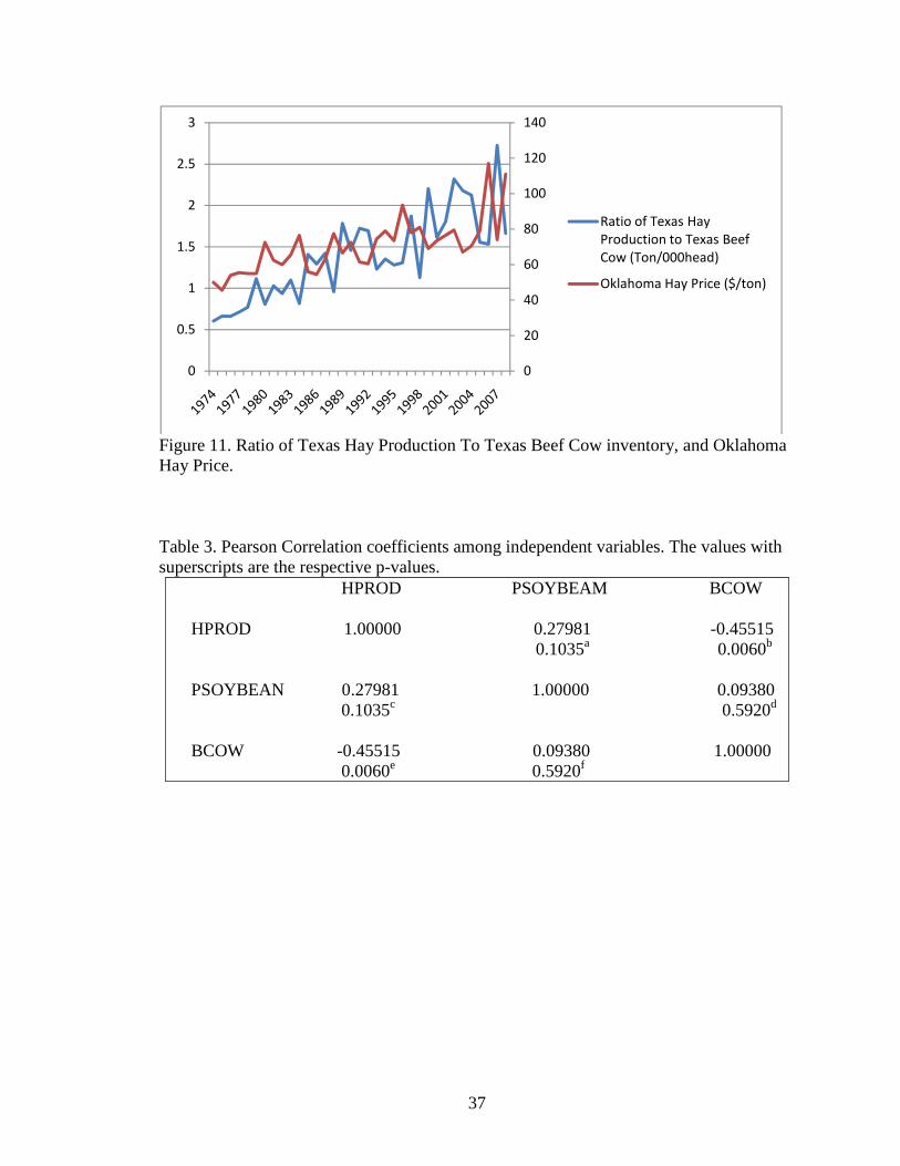
Oklahoma hay price ............................................................................................36 11. Ratio of Texas Hay Production to Texas Beef Cow inventory, and Oklahoma hay price………………………………………………………………………. 37
1
CHAPTER I
INTRODUCTION
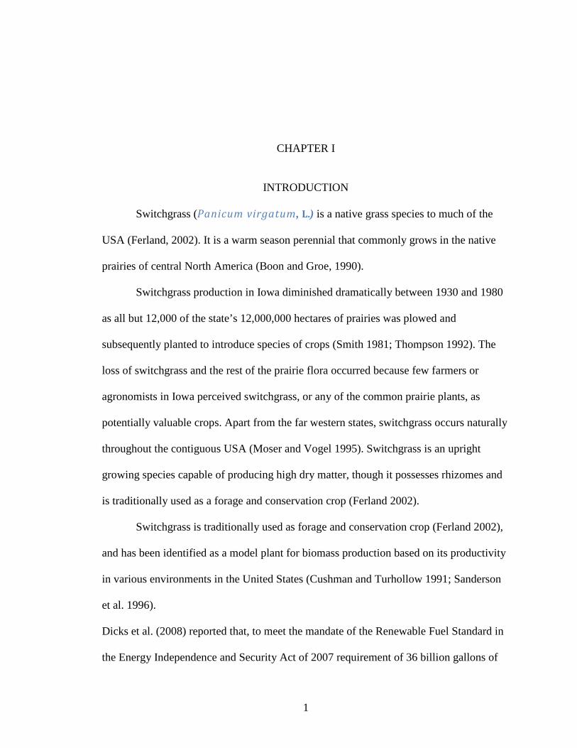
Switchgrass (Panicum virgatum, L.) is a native grass species to much of the
USA (Ferland, 2002). It is a warm season perennial that commonly grows in the native
prairies of central North America (Boon and Groe, 1990).
Switchgrass production in Iowa diminished dramatically between 1930 and 1980
as all but 12,000 of the state’s 12,000,000 hectares of prairies was plowed and
subsequently planted to introduce species of crops (Smith 1981; Thompson 1992). The
loss of switchgrass and the rest of the prairie flora occurred because few farmers or
agronomists in Iowa perceived switchgrass, or any of the common prairie plants, as
potentially valuable crops. Apart from the far western states, switchgrass occurs naturally
throughout the contiguous USA (Moser and Vogel 1995). Switchgrass is an upright
growing species capable of producing high dry matter, though it possesses rhizomes and
is traditionally used as a forage and conservation crop (Ferland 2002).
Switchgrass is traditionally used as forage and conservation crop (Ferland 2002),
and has been identified as a model plant for biomass production based on its productivity
in various environments in the United States (Cushman and Turhollow 1991; Sanderson
et al. 1996).
Dicks et al. (2008) reported that, to meet the mandate of the Renewable Fuel Standard in
the Energy Independence and Security Act of 2007 requirement of 36 billion gallons of
2
ethanol production in the year 2022, 24.7 million acres would be used to produce 109
million tons of switchgrass in 2025. Using only the 450 million acres of cropland
currently available in the United States, the increased switchgrass acreage would reduce
hay acres by 15.4 million, leading to a 13.1 million head reduction in beef cows.
The federal mandate, together with the comparative advantage and the potentials
of switchgrass will switch most of the cropland used for hay to the production of
switchgrass.
This research will determine the potential impact of switchgrass production on
Oklahoma hay markets.
Background
Understanding the hay market is important because of the significance of hay to
the economy of the agriculture sector. Information about acreage, yield, and price can
help hay producers in anticipating the demand for their product, livestock producers in
comprehending the supply of their major input, and policymakers in predicting the effects
of proposed policies on the hay market. The emerging potential of switchgrass is a
concern for hay markets because of the probability that farmers may use their land to
produce switchgrass rather than hay if switchgrass is more profitable.
Because reliable information on hay market price response was not available for
the study by Dicks et al, the predicted effect on beef cows came from a simplistic
estimate that reduced beef cow numbers based solely on the tons of forage reduced. In
that study, forage was reduced as land was shifted to switchgrass. Since each cow needs
approximately 1,000 pounds of forage per month, replacing forage with switchgrass-for-
3
ethanol would correspondingly reduce the number of cows that could be produced unless
cow prices increase substantially. To fully understand the impacts of biofuel mandates on
cattle markets a linkage between cattle numbers and hay prices needs to be established.
Previous estimates of the effect of biofuel mandates on hay and livestock markets (such
as those by Dicks et al. 2008) did not consider the price impacts on those markets
because good information was not available. This research will provide more realistic
estimates of those effects by more fully considering the price responsiveness of producers
to competing alternatives for a limiting resource, land. Increased profitability of
switchgrass production will bid resources (especially land) away from hay production.
Farmers aim to maximize returns and will look for alternative crops that will yield
higher profits. The findings from this research will help hay and livestock producers and
policymakers better anticipate changes in the market for hay in Oklahoma as switchgrass
production increases.
Objectives
The overall objective of this thesis is to determine the potential impact of
increased switchgrass production on Oklahoma hay markets.
Specific objectives are to:
1) determine the demand for hay in Oklahoma;
2) determine the impact of the level of hay production in surrounding states on
Oklahoma hay price; and
3) determine the production options between hay and switchgrass in Oklahoma
based on profitability.
4
CHAPTER II
LITERATURE REVIEW
This chapter provides a brief background on switchgrass and hay markets and their
potential contributions to the economy of the agricultural sector. It reviews the limited
studies related to switchgrass and hay markets.
Potentials of switchgrass production
In recent years switchgrass has shown great potential for use in the production of
fuel ethanol from cellulosic biomass (Lynd et al. 1991). Research in Alabama
demonstrated that very high dry matter yields can be achieved with switchgrass in the
southern USA (Maposse et al. 1995). Farmers in this area can therefore produce
switchgrass for either biomass or forage.
When combining its uses of forage, conservation, and biofuel production, farming
systems based on switchgrass could become an economic boon for farmers interested in
sustainable and profitable farming enterprises (Ferland 2002). Switchgrass has been
identified as a model plant for biomass production based on its productivity in various
environments in the United States (Cushman and Turhollow 1991; Sanderson et al.
1996).
An ideal biomass system would consist of one warm-season and one cool-season
perennial grass, a legume, and an annual warm-season grass (Cushman and Turhollow,
5
1991). Despite such ecologically sound advice, virtually all work in the past decade has
emphasized switchgrass alone (McLaughlin et al. 1997).
The commercialization of cellulosic-based ethanol (ethanol that comes from
feedstocks such as switchgrass, corn stover, wheat straw, and wood products residues)
could have an even greater impact on the agricultural industry (Epplin 1996). Potential
conversion rate of 75 gallons or more from each ton of switchgrass coupled with
expected switchgrass yields of 4-6 tons/acre have led to excitement over the future role of
dedicated biofuel crops in the regions agriculture.
President George W. Bush mentioned switchgrass in both his 2006 and 2007 State
of the Union speeches (Whitehouse 2007). He announced the ambitious “20 in 10”
initiative that calls for reducing gasoline demand 20% in 10 years by producing 35 billion
gallons of ethanol (which would replace roughly 15% of gasoline), and improving the
Corporate Average Fuel Economy (CAFE) standards to reduce demand by 8.5 billion
gallons of gasoline, or 5% of the current demand.
What will be the impact on other crops – including hay, and thus livestock
production - of converting a greater part of Oklahoma farmland into switchgrass?
Oklahoma biofuel production would exceed currently available feedstock, even when
competing uses for livestock are ignored (Kenkel and Ragan, 2007). They note that,
biofuel production could stimulate a substantial increase in feed grain production. This
shift would have major impacts on the livestock industry since much of the production
would come from land currently used for hay and pasture production shifting into feed
grains (Kenkel and Ragan, 2007). Similarly, cellulosic ethanol technologies could greatly
increase ethanol production, which would impact existing crop and forage production.
6
Policy issues
The Renewable Fuel Standard mandates in the Energy Independence and Security
Act of 2007 (EISA 2007) will require 36 billion gallons of ethanol to be produced in
2022, 16 billion gallons of which is to be produced from cellulosic feedstocks. To meet
this mandate, 24.7 million acres would be used to produce 109 million tons of
switchgrass in 2025. Using only the 450 million acres of cropland currently available in
the United States, the increased switchgrass acreage would reduce hay production by 15.4
million hay acres leading to a 13.1 million head reduction in beef cows (Dicks et al.
2008). The most emphasized crop for this purpose is switchgrass. Research sponsored by
the Bioenergy Feedstock Development Program at the Oak Ridge National Laboratory
evaluated more than 30 species of crops on research plots on a wide range of soil types in
more than 30 sites across seven states (Wright 2007). Based on these trials, switchgrass
was selected as a model species.
The wide support from Americans for expansion of the ethanol industry led to the
expansion of the Renewable Fuels Standard (RFS) mandated in the Energy Independence
and Security Act of 2007 (EISA 2007). This wide support was the result of the optimism
associated with achieving energy independence and rural economic development
(Herndon 2008), but was apparently enacted without critical assessments of the
agricultural impacts of attempting to achieve them. In particular, reduced hay production
will likely increase hay prices which could make hay less affordable to livestock farmers,
with a secondary consequence of reduced livestock numbers.
7
Impacts of Switchgrass Production on Pasture Land, Cattle herd and Hay Price
The overwhelming majority of range and pasture acres are used to produce forage
to feed roughly 100 million cattle and calves. A biofuel industry would bid resources
from current use with possible negative impacts on some agricultural sectors. Dicks et al.
(2008) found that the majority of the land required to meet the biofuel potential would be
converted from land currently producing hay, cotton and wheat in the southeast.
Converting this land to biofuel feedstock would negatively impact the cattle industry
since hay production and marketing would be affected, and hay prices would rise. This
research will determine the impact of switchgrass production on hay markets in
Oklahoma.
What is hay?
Hay is one of the methods of preserving forage crops for use by livestock at a
future date when feed is scarce. Legumes and grasses, including cereals, are the main hay
crops. The crops meant for hay preparation are harvested just before flowering or at the
early flowering stage when the crops are leafy, more nutritious, and less fibrous and have
lower water content. There is also standing hay or in-field-hay which is conserved by
allowing the crops to dry while standing in the field
Because grains are consumed by both humans and animals, reducing grain
consumption by animals by using grain as a food supplement, with hay as the main food,
reduces the total demand for grains and thus costs to the livestock producers. In many
instances, livestock are able to access forage crops through pasture grazing. However,
8
most forage crops are not available throughout the year, so preserving some of the forage
as hay for use in the dormant season ensures animal feed security and help prevent over-
reliance on grains.
Demand and supply for hay
Understanding interactions between supply and demand for hay is important
because of hay’s significance to the agricultural sector and the economy, and because hay
is an important crop on highly erodible soils (Bazen et al. 2008).
Hay production in the U.S. was 145.67 million tons valued at $18.78 billion with
an average price of $157 per ton (USDA National Agricultural Statistics Service 2008).
Tennessee has the most erodible cultivated cropland in the United States (Denton, 2000),
so hay is one of the most economically important crops produced in the state (U.S.
Department of Agriculture, 2004). Cross (1999) observed that the upward trend in
Tennessee hay acreage since 1980 is due to an increasing number of farmers who were
searching for alternative production activities, such as hay, pasture and livestock, to
replace row crops on erodible soils. Hay ranked tenth in value of receipts in Tennessee at
$49.25 million in 2006 and cattle and calf production ranked first at $500 million. In
2003, hay ranked second in value of production at $262 million and averaged $248
million over a five year period from 2002 to 2006. Underscoring the importance of hay in
Tennessee was the state’s national ranking of fourth in the production of other hay
(excluding alfalfa) at 4.25 million tons in 2006 (U.S. Department of Agriculture 2007).
9
Characteristics of hay markets must be understood in order to be able to quantify
the demand and supply relationship for hay, since hay markets are usually localized due
to the weight and bulky physical characteristics of hay (Basen et al. 2008).
Although hay is not a homogeneous commodity, in most livestock production
situations, the various types of forages that are used to produce hay are close substitutes,
with the exception of alfalfa hay. Alfalfa is a differentiated hay product used mostly by
dairy and equine producers, but its price tends to move proportionally with other hay
prices. Thus, for modeling purposes alfalfa and other hay can be aggregated as in
Shumway’s (1983) study of Texas field crops and treated as a composite commodity
(Nicholson 2005) called hay. In 2002, 47,000 operations within Texas produced forage,
while on the demand side, 50,000 operations were involved in beef and dairy production
with another 24,000 equine operations (U.S. Department of Agriculture 2004).
Even though there are no national and state central markets for hay (Cross 1999),
buyers and sellers seem to be aware of the current prices in their area (Bazen et al. 2008).
Hay producers are typically assumed to be price takers (Shumway 1983) because of the
large numbers of sellers and buyers. Even though hay and livestock producers have
avenues for price determination in the short run, they have little information about what
causes supply and demand for hay to change from year to year (Bazen et al. 2008).
Hay Price Determinants
The quality of hay produced should affect the price buyers will pay for it. Thus
the price and quality relationship is important to both producers and buyers. Producers
must know the quality of their hay to accurately estimate its value and realistically
10
formulating an asking price. Livestock producers, on the other hand, must know the
quality of hay in order to assess its value as a production input and to accurately develop
a realistic bid price. Even though there are objective measures of hay quality, most hay
buyers use subjective evaluation such as visual appearance, feel and smell to determine
quality grade.
The type of hay whether alfalfa, grass, wheat or a combination of all, could affect
its price. In Oklahoma, while alfalfa hay price ranges from $90 to $200 per ton depending
on bale size and quality, wheat hay and grass hay in similar condition ranges from $85 to
$130 per ton and $55 to $100 per ton respectively (Oklahoma Department of Agriculture
2009).
Price of hay can also be affected by current and past stocks. Hay stocks stored on
farms as of May 1, 2009 totaled 22.1 million tons, up 2% from 2008. Disappearance from
December 1, 2008 to May 1, 2008 totaled 81.6 million tons, compared with 82.5 million
tons for the same period in 2009. Hay stocks decreased from 2008 across most of the
Great Plains and Rocky Mountain States. Texas and Oklahoma had the largest decrease
due in part to lower hay production in 2008. In addition, dry weather during the fall and
winter 2008 resulted in poor pasture conditions which increased supplemental hay
feeding (NASS-USDA, Louisiana Farm Reporter 2009). Thus hay price in these states
were comparatively higher in 2008 than 2009.
Recent Hay Production Levels in Oklahoma
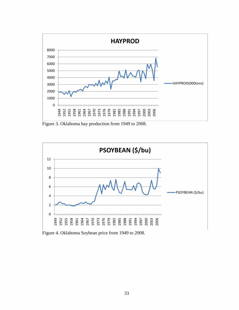
Even though there have been intermittent fluctuations, Oklahoma hay production
has been increasing since the late 1940s (Figure 3). In Oklahoma, 3.14 million and 2.91
11
million acres of hay were harvested in 2007 and 2008, respectively. Oklahoma hay
production was estimated to be 6.858 million tons in 2007 and 5.536 million tons in
2008, with an average price of $74/ton in 2007 and $111/ton in 2008.
12
CHAPTER III
METHODOLOGY
Conceptual Framework
The overall objective of this research is to determine the impact of switchgrass
production on Oklahoma hay markets. Agricultural producers and land owners will
decide whether to produce switchgrass or hay, considering the net economic returns of
each. The research assumes a profit maximizing firm chooses whether to produce
switchgrass or other hay crops.
The demand equation for hay is modeled using ordinary least squares (OLS)
estimates while the profitability decision on whether to produce hay or switchgrass is
modeled using linear programming (LP).
The demand equation is an inverse demand function with hay price as the
dependent variable, That equation is used to predict the hay price which used in the LP
model as the objective value for hay.
Data Sources
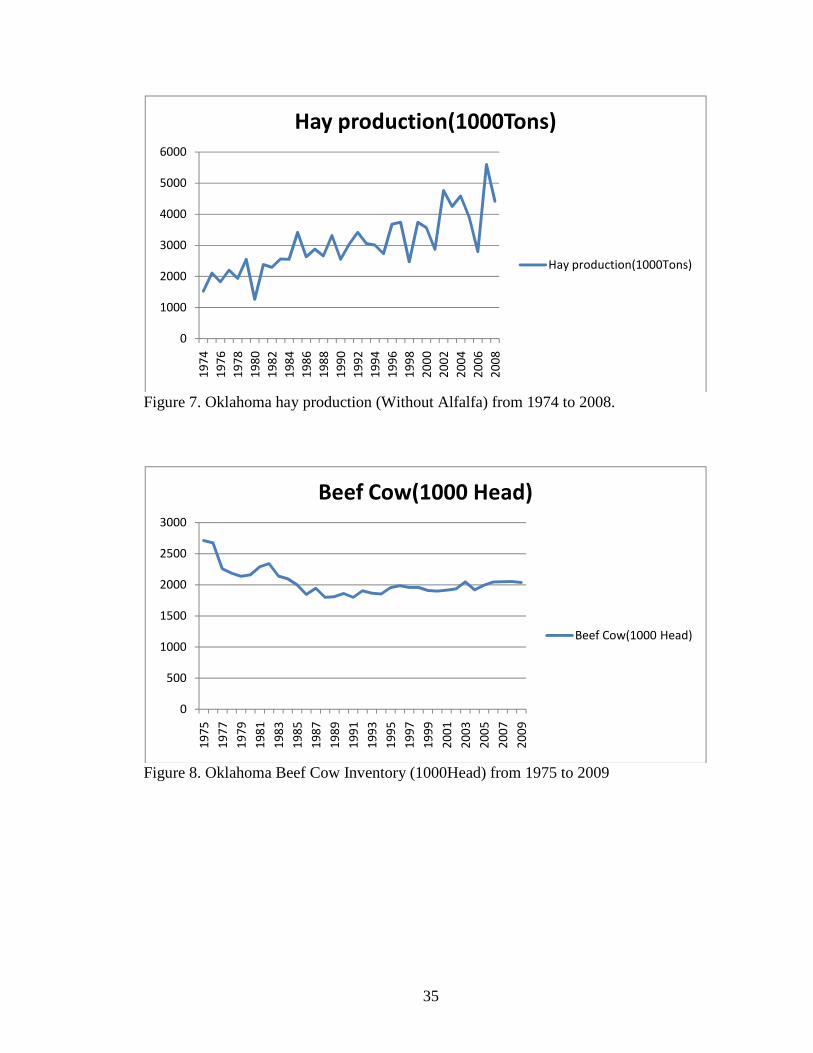
Data on hay production, price of hay, cattle and calves inventory, beef cow
inventory, and soybean price for Oklahoma, as well as Texas and Arkansas, were
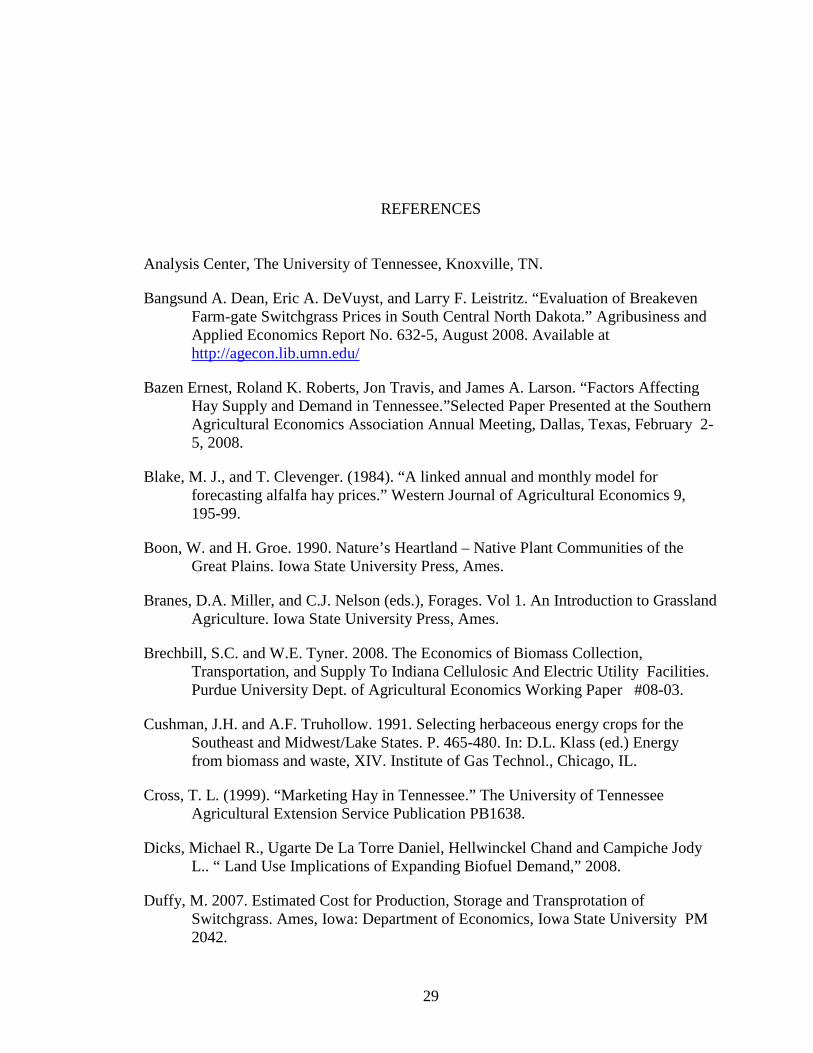
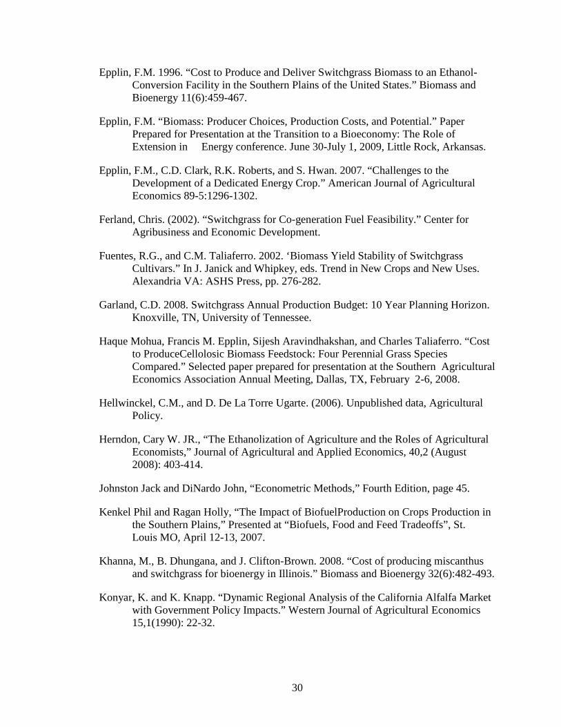
obtained from USDA-NASS. Figures 1 to 8 show the trend in the various data across
13
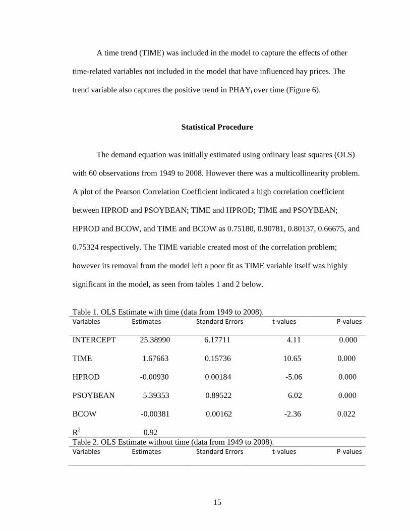
specific periods of time. The initial OLS equation (tables 1 and 2) was estimated using
data from 1949 to 2008. However due to the problems of multicollinearity and
unexpected signs of some of the estimated coefficients, data from 1974 to 2008 were
used for hay price (PHAY), hay production (HPROD), and soybeans price (PSOYBEAN)
while data from 1975 to 2009 were used for beef cow inventory (BCOW). Beef cow
numbers are reported on January 1, so those numbers are assumed here to most closely
apply to data for the previous year.
Hay Demand
Konyar and Knapp (1990) modeled price of hay as a function of alfalfa
production, feed, livestock prices, and animal inventory. Blake and Clevenger (1984)
modeled quantity as a function of corn price and a trend. Bazen et al. (2008) modeled
Tennessee hay price as a function of hay production, price of soybean, cattle and calf
inventory, income, and time trend and found all variables attaining their expected signs.
Blake and Clevenger (1984) and Myer and Yanagida (1984) observed that an
inverse demand function with hay price as the dependent variable is appropriate when
supply is predetermined. Hay supply could be predetermined by the current year
plantings, harvesting and weather.
For this study, the inverse demand function was specified as:
PHAY = f(TIME, HAYPROD, PSOYBEAN, BCOW)
with the empirical form as :
PHAYt = β0 + β1TIMEt + β2HAYPRODt + β3PSOYBEANt + β4BCOWt+1 + et
14
Where PHAY is the annual price of hay ($/ton) in Oklahoma; TIME is a time trend with
1974 = 1, 1980 = 2,…, and 2008 = 35; HAYPROD is Oklahoma hay production other
than alfalfa (1,000 tons); PSOYBEAN is Oklahoma soybean price ($/bu); and BCOW is
Oklahoma beef cow inventory (1,000 head) on January 1 of the following year; et is a
random error; βi (i = 0,…, 5) and are parameters to be estimated; t is a subscript for the
current year; and t+1 is a subscript for the following year.
Demand Hypothesis
The coefficient of HAYPROD (β2) was expected to be negative in order to be
consistent with a negatively sloped industry demand curve (Blake and Clevenger 1984;
Myer and Yanagida 1984). The higher the price of the commodity, the lower the quantity
of the commodity to be demanded.
The coefficient of PSOYBEAN is hypothesized to be positive. Soybean price was
considered in the model to represent the price of a substitute (protein supplement). Thus
the price of soybeans is expected to be positively related to the hay price. Prices of
ingredients in feed rations tend to move together because the ingredients are generally
good substitutes (Blake and Clevenger 1984).
The coefficient of BCOW is expected to be positive. An increase in the price of
beef would act as an incentive for livestock producers to increase input use (Nicholson,
2005) as they build their herds. Thus beef cow producers would build their herds in
anticipation for future profits which will consequently increase their demand for hay,
thus, increasing the price of hay.
15
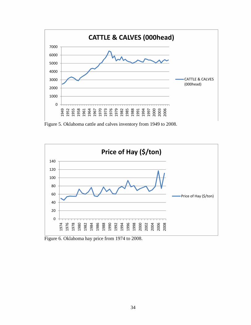
A time trend (TIME) was included in the model to capture the effects of other
time-related variables not included in the model that have influenced hay prices. The
trend variable also captures the positive trend in PHAYt over time (Figure 6).
Statistical Procedure
The demand equation was initially estimated using ordinary least squares (OLS)
with 60 observations from 1949 to 2008. However there was a multicollinearity problem.
A plot of the Pearson Correlation Coefficient indicated a high correlation coefficient
between HPROD and PSOYBEAN; TIME and HPROD; TIME and PSOYBEAN;
HPROD and BCOW, and TIME and BCOW as 0.75180, 0.90781, 0.80137, 0.66675, and
0.75324 respectively. The TIME variable created most of the correlation problem;
however its removal from the model left a poor fit as TIME variable itself was highly
significant in the model, as seen from tables 1 and 2 below.
Table 1. OLS Estimate with time (data from 1949 to 2008). Variables Estimates Standard Errors t-values P-values
INTERCEPT 25.38990 6.17711 4.11 0.000
TIME 1.67663 0.15736 10.65 0.000
HPROD -0.00930 0.00184 -5.06 0.000
PSOYBEAN 5.39353 0.89522 6.02 0.000
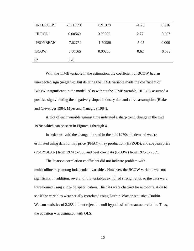
BCOW -0.00381 0.00162 -2.36 0.022 R2 0.92 Table 2. OLS Estimate without time (data from 1949 to 2008). Variables Estimates Standard Errors t-values P-values
16
INTERCEPT -11.13990 8.91378 -1.25 0.216
HPROD 0.00569 0.00205 2.77 0.007
PSOYBEAN 7.62750 1.50980 5.05 0.000
BCOW 0.00165 0.00266 0.62 0.538
R2 0.76
With the TIME variable in the estimation, the coefficient of BCOW had an
unexpected sign (negative), but deleting the TIME variable made the coefficient of
BCOW insignificant in the model. Also without the TIME variable, HPROD assumed a
positive sign violating the negatively sloped industry demand curve assumption (Blake
and Clevenger 1984; Myer and Yanagida 1984).
A plot of each variable against time indicated a sharp trend change in the mid
1970s which can be seen in Figures 1 through 4.
In order to avoid the change in trend in the mid 1970s the demand was re-
estimated using data for hay price (PHAY), hay production (HPROD), and soybean price
(PSOYBEAN) from 1974 to2008 and beef cow data (BCOW) from 1975 to 2009.
The Pearson correlation coefficient did not indicate problem with
multicollinearity among independent variables. However, the BCOW variable was not
significant. In addition, several of the variables exhibited strong trends so the data were
transformed using a log-log specification. The data were checked for autocorrelation to
see if the variables were serially correlated using Durbin-Watson statistics. Durbin-
Watson statistics of 2.288 did not reject the null hypothesis of no autocorrelation. Thus,
the equation was estimated with OLS.
17
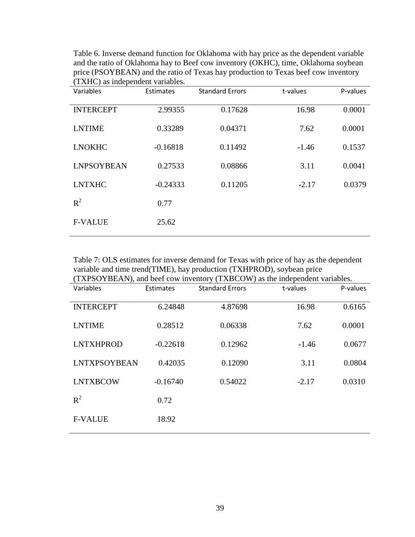
The Oklahoma hay price (PHY), time trend (TIME), ratio of Oklahoma hay
production to Oklahoma beef cow inventory (OKHC), Oklahoma soybean price, and ratio
of Texas hay production to Texas beef cow inventory(TXHC) were estimated using
Oklahoma hay price as the dependent variable to find out the effect on Oklahoma hay
price (Table 8).
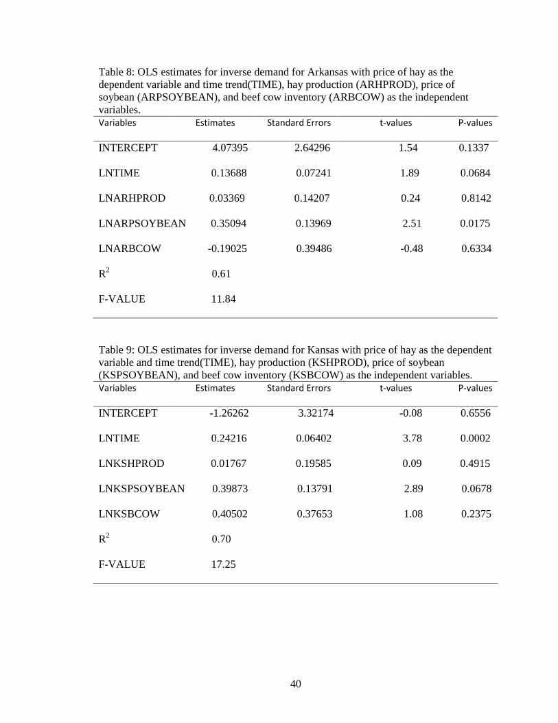
The final model developed for Oklahoma hay demand was tested on some states
that border Oklahoma (Kansas, Texas, and Arkansas) to find out the validity of the model
in those states (Tables 9,10, and 11).
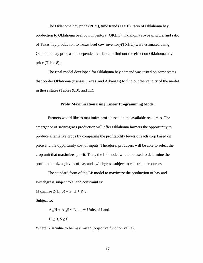
Profit Maximization using Linear Programming Model
Farmers would like to maximize profit based on the available resources. The
emergence of switchgrass production will offer Oklahoma farmers the opportunity to
produce alternative crops by comparing the profitability levels of each crop based on
price and the opportunity cost of inputs. Therefore, producers will be able to select the
crop unit that maximizes profit. Thus, the LP model would be used to determine the
profit maximizing levels of hay and switchgrass subject to constraint resources.
The standard form of the LP model to maximize the production of hay and
switchgrass subject to a land constraint is:
Maximize Z(H, S) = PHH + PSS
Subject to:
A11H + A12S ≤ Land ⇒ Units of Land.
H ≥ 0, S ≥ 0
Where: Z = value to be maximized (objective function value);
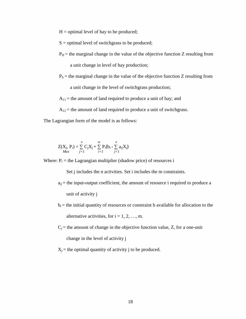
18
H = optimal level of hay to be produced;
S = optimal level of switchgrass to be produced;
PH = the marginal change in the value of the objective function Z resulting from
a unit change in level of hay production;
PS = the marginal change in the value of the objective function Z resulting from
a unit change in the level of switchgrass production;
A11 = the amount of land required to produce a unit of hay; and
A12 = the amount of land required to produce a unit of switchgrass.
The Lagrangian form of the model is as follows:
n m n
Z(Xj, Pi) = ∑ CjXj + ∑ Pi�bi - ∑ aijXj� Max j=1 i=1 j=1
Where: Pi = the Lagrangian multiplier (shadow price) of resources i
Set j includes the n activities. Set i includes the m constraints.
aij = the input-output coefficient, the amount of resource i required to produce a
unit of activity j
bi = the initial quantity of resources or constraint b available for allocation to the
alternative activities, for i = 1, 2, …, m.
Cj = the amount of change in the objective function value, Z, for a one-unit
change in the level of activity j
Xj = the optimal quantity of activity j to be produced.
19
Switchgrass and Hay Yields and Acreage Requirements
The opportunity cost of land, and the expected yield and price per unit will
determine the production options between hay and switchgrass for this study.
Switchgrass yield is estimated to range from 2.23 tons per acre, as reported by
Perrin et al. (2008) from field level studies in the northern plains to 6.45 tons per acre, as
budgeted by Garland (2008) for Tennessee. Perrin et al. (2008) originally estimated
production costs of $60 per ton based on field level studies but they reported a cost of
$54 per ton based on extrapolated costs over a ten year stand life.
Epplin et al. (2007) reported a switchgrass yield from 3.75 tons per acre to 6.50
tons per acre, with an estimated farm gate production cost between $37 per ton and $53
per ton. The lowest cost of $37 per ton from their study depended critically on the
assumption that harvest could extend over at least eight months. The extended harvest
season allows for a substantially lower investment in harvest machines resulting in lower
fixed costs per harvested ton and also lower storage costs.
Fuentes and Taliaferro (2002) reported switchgrass yields from variety trials
conducted over seven years at two locations in Oklahoma. They found an average annual
yield of 7.2 tons per acre from stands that included a combination of varieties Alamo and
Summer. Haque et al. (2008) reported a mean annual yield of 5.5 tons per acre with one
harvest per year and production cost of $47 per ton for Oklahoma. Based on their
estimate of 5.5 tons per acre, 0.182 acre of land will be required to produce a ton of
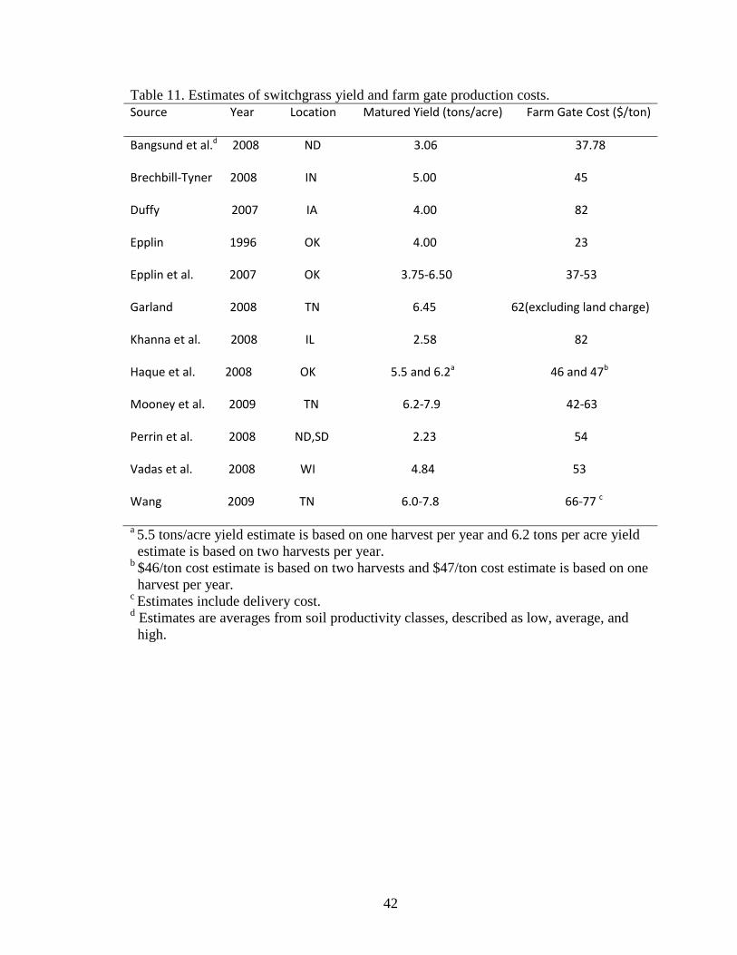
switchgrass. Table 12 includes a summary of switchgrass yield and production cost
estimates from various studies. Some of these were reported by Epplin (2009). The table
indicates that yield estimates for switchgrass production in Oklahoma and Tennessee are
20
higher than those from other states. Thus, Oklahoma and Tennessee are very promising
for switchgrass production and can bid land away from some of the traditional crops
including hay.
Determining the yield and acreage requirement for hay is difficult because hay is
not as homogeneous as other crops. Grass hay can be produced from a variety of grasses
which have different growth requirements, thus producing different yields. This
characteristic makes it difficult to aggregate hay yield and acreage requirement as a
single crop. Although, USDA/NASS reports the annual aggregate yield per acre of hay as
a single crop but this does not reflect the actual yield of the individual grass species used
in producing the hay. USDA/NASS reports a mean annual all-hay yield of 1.8 tons per
acre from 2000 to 2008. In 2008, USDA/NASS reported 2,600,000 harvested acres of
hay (all-hay minus alfalfa). Haque et al. (2008) estimated the mean annual yield (dry tons
per acre) of Burmudagrass, Lovegrass, and Flaccidgrass in Oklahoma to be 3.38, 3.53,
and 4.5, respectively, for one harvest per year; and 4.8, 4.28, and 4.98, respectively, for
two harvests per year. These figures are the means calculated from the means reported
based on quantities of nitrogen per acre application. The respective costs of production
($/ton) are 57.00, 50.50, and 50.25 for one harvest per year; and 48.25, 48.75, and 48.25
for two harvests per year. If these grasses are produced as grass mix hay, they would have
aggregate yields of 3.80 tons per acre for one harvest a year and 4.69 tons per acre for
two harvests a year with production costs of $52.58 per ton for one harvest and $48.42
per ton for two harvests. Based on the yield from the two harvests a year, one ton of dried
hay mix will require 0.213 acre of land.
21
Switchgrass and Hay Prices
Data and information on switchgrass prices are not currently available because
markets for biomass are absent for much of the United States. Some studies including
Bangsund et al. (2008) have estimated breakeven farm-gate switchgrass prices. However,
for a switchgrass cropping systems to become commercially viable, the price paid to
producers per ton of biomass must be high enough to bid land away from traditional farm
enterprises, rather than simply offsetting production costs. Recent studies in Oklahoma
indicate good switchgrass yields with comparatively lower production costs (table 13).
Thus an attractive switchgrass price will likely bid away land currently used to produce
some traditional crops including hay.
Oklahoma hay prices have been fairly stable over time, though there have been
short-term fluctuations in response to production levels. USDA/NASS reports a mean
annual all-hay price of $83.11 per ton from years 2000 to 2009. This study estimates the
2008 Oklahoma grass hay price to be $91.50 per ton.
The LP Procedure
The LP model was used to maximize returns from the production of hay and
switchgrass. Excel Solver was used to indicate the production of hay and switchgrass that
will yield maximum profit based on the available resource (land) holding all other factors
constant. The objective function of the LP model is as follows:
Maximize Z = PHH + PSS
Subject to: A11H + A12S ≤ Land
22
To produce one dry ton of switchgrass, 0.182 acre of land is required, while 0.213 acre of
land is required to produce one dry ton of hay that is sold for $91.50. The study assumes
total available land is 2,600,000 acres as reflected in the 2008 report from NASS-USDA
as the harvested acres of hay (excluding alfalfa). Switchgrass price information is rarely
available in Oklahoma and therefore, the price of switchgrass will be parameterized in
this modeling process. A switchgrass price that is lower than that of the hay price will be
used and then parameterized to find the point at which it will make switchgrass more
profitable than hay.
23
CHAPTER IV
FINDINGS
Demand Equation
The Pearson Correlation matrix (Table 3) did not show any problem of
multicollinearity, suggesting that the demand equation can be represented by a recursive
model. Using a log-log specification, the Durbin-Watson statistic of 2.288 led to failing
to rejcet the null hypothesis of no autocorrelation. Thus, the demand equation was
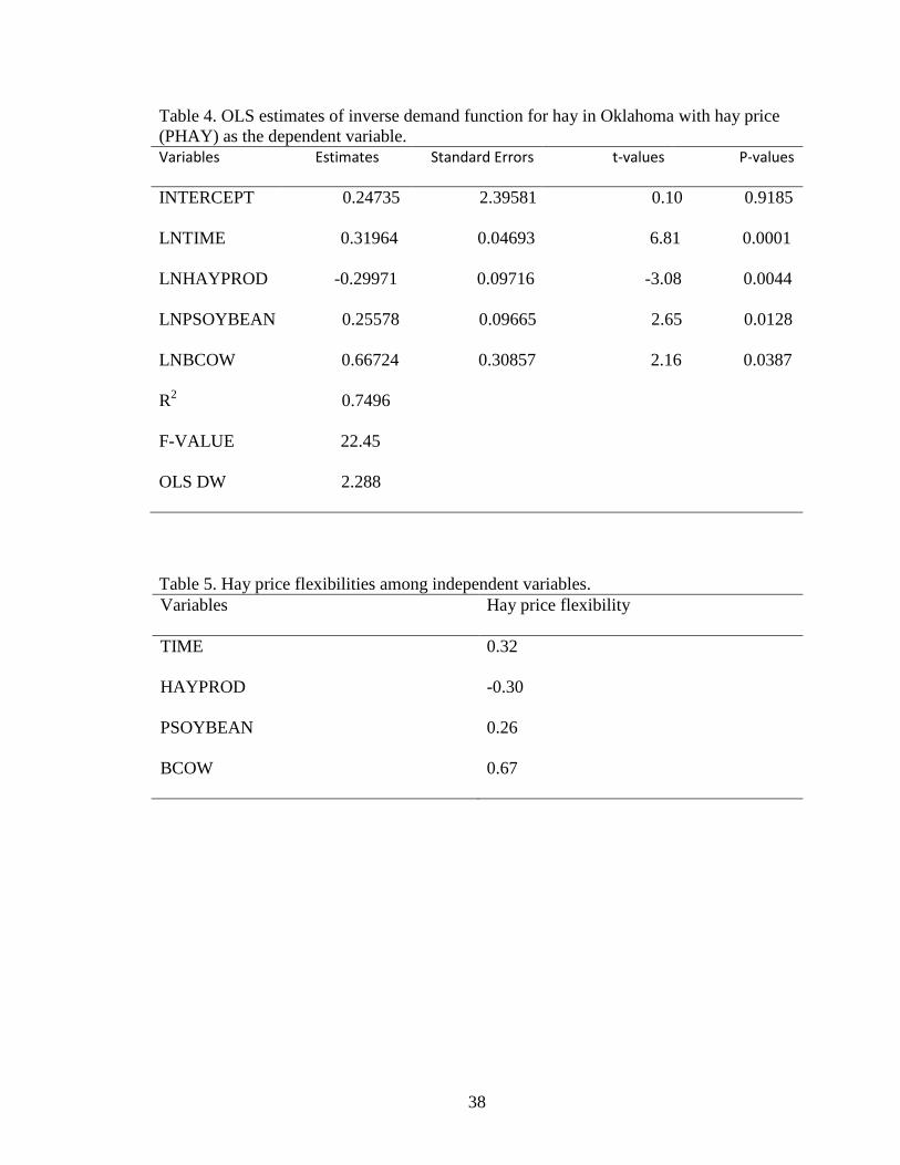
estimated with OLS (Table 4).
All coefficients were significant at the 5% level with the appropriate signs. The
negative sign of the coefficient for hay production confirms a negatively sloped demand
curve in which quantity demanded increases as price decreases. Soybeans price appeared
to be positively related to the hay price because they are substitutes. An increase in the
soybeans price relative to the hay price creates an incentive for beef cow producers to
feed their cows more hay, thus increasing hay demand which will result in an increase in
the price of hay. An increase in the beef cow inventory leads to an increase in their
demand for hay with a consequent increase in the price of hay.
The coefficients of the variables represent marginal changes in the price of hay
with respect to a unit change in the respective variable. Therefore, a unit increase in the
level of hay production will cause a $0.30 decrease in the price of hay, and hay price
24
increases $0.26 and $0.67, respectively, for one unit increases in the soybean price
(PSOYBEAN) and the beef cow inventory (BCOW).
The final inverse demand function obtained from the OLS is;
Ln(PHAYt) = β0 + β1Ln(TIMEt ) + β2Ln(HPRODt ) + β3Ln(PSOYBEANt ) +
β4Ln(BCOWt+1) + et
Price flexibilities show the degrees of responsiveness in the price of hay (PHAY)
to a percentage change in hay production, price of soybeans, and beef cow inventory
(table 5). It should be noted that the slopes of the log-log specifications are the direct
estimates of (constant) elasticities (Johnston and DiNardo, 1997), but for inverse demand
functions with log-log specifications, the coefficients of the independent variables are the
price flexibilities as used in Bazen et al. (2008). Thus a one-percentage increase in the
level of hay production will cause approximately a 0.30% decrease in the price of hay. A
one-percent increase in soybeans price was associated with a 0.26% increase in the price
of hay, and a one-percent increase in beef cow inventory was associated with a 0.67%
increase in the price of hay. Hay price is unresponsive to time, hay production, soybeans
price, and beef cow inventory.
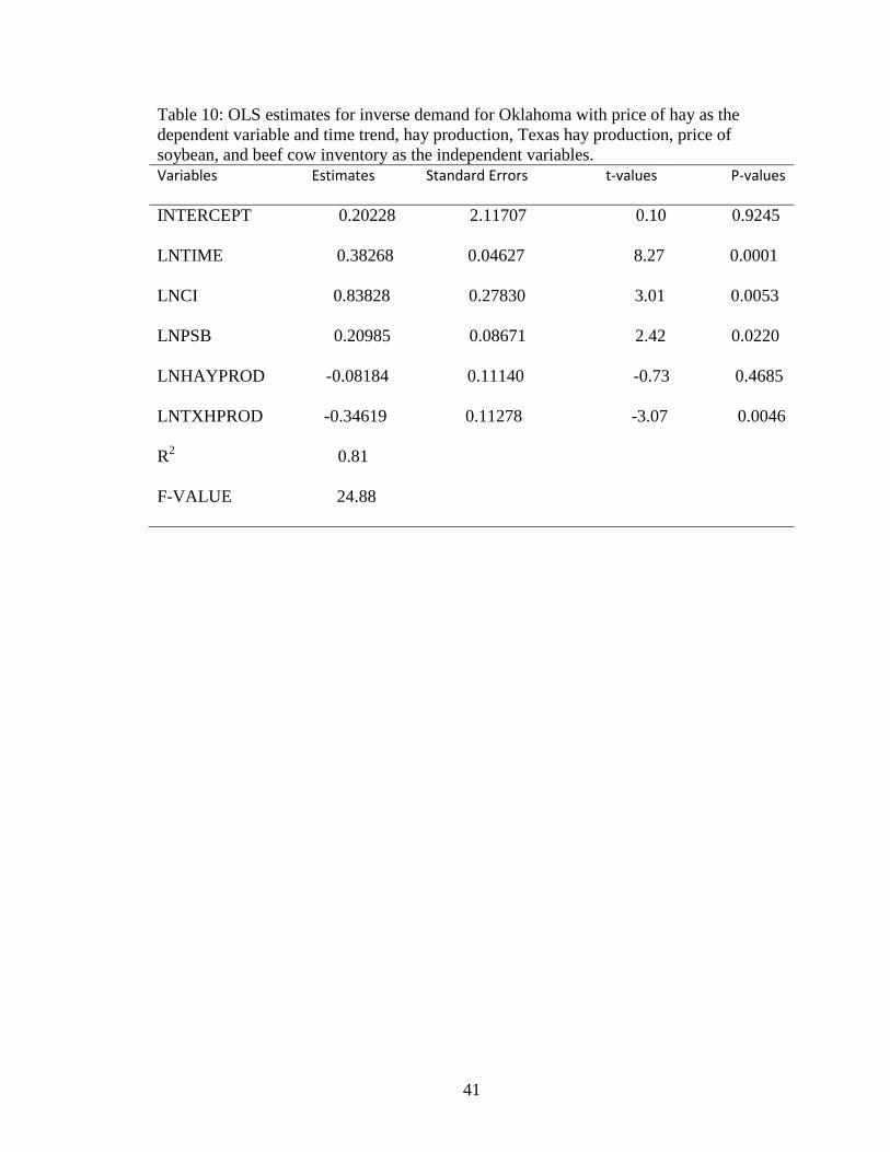
Texas hay production and the ratio of Texas hay production to Texas beef cow
inventory were alternatively added to the Oklahoma model and both appeared to be more
significant in the model than Oklahoma hay production.
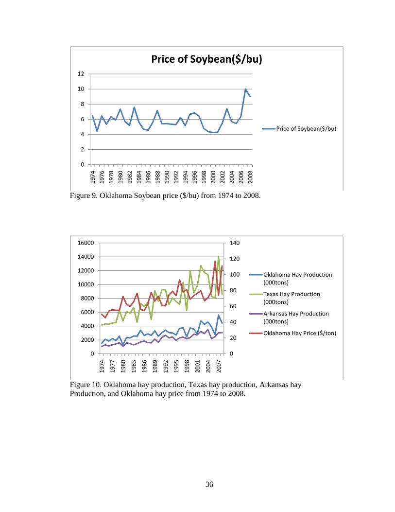
Figure 10 compares the levels of Oklahoma hay production, Texas hay
production, and Arkansas hay production with Oklahoma hay price. The production
levels in these states appear to move in the same direction. The higher the quantity of hay
produced in these states, the lower the price of hay in Oklahoma.
25
Hay Price Predictive Model for Oklahoma
Table 4 shows the parameter estimates of the inverse demand for Oklahoma hay
production with hay price (PHAY) as the dependent variable and time trend (TIME), hay
production (HPROD), soybeans price (PSOYBEAN), and beef cow inventory (BCOW)
as dependent variables, which is conceptually given as;
LNPHAYt = β0 + β1LNTIME t + β2LNHPRODt + β3LNPSOYBEANt + β4LNBCOWt+1 +
et …………………………………………………………………………………………(1)
Empirically, equation (1) becomes,
LNPHAYt = 0.24735 + 0.31964(LNTIMEt) - 0.29971(LNHPRODt) +
0.25578(LNPSOYBEANt ) + 0.66724(LNBCOWt+1) + et ……………………………..(2)
Where et is described as white noise since ∑et= 0. Thus, Oklahoma hay price could be
predicted by equation (2). Users of this model should be reminded that the time variable
was from 1 to 35 (1974=1, 1975=2,.., 2008=35), therefore, any number of years from
2008 that would be predicted must be added on to 35 for the time variable and so for
2009, the time variable would be 36. Thus this model estimates 2008 grass hay price to
be $91.50.
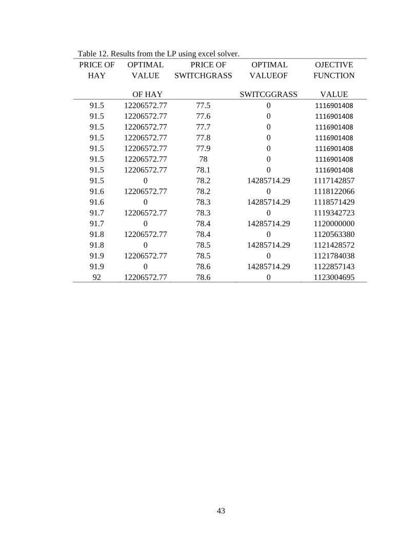
LP Results
Analyses were based on only a land constraint and prices while holding all other
factors constant. Table 13 summarizes the results from the LP procedure using excel
solver. At a price of $91.50/ton for hay and $77.50/ton for switchgrass, it would be
profitable to produce hay instead of switchgrass. Parameterizing the price of switchgrass
26
by adding $0.10 to $77.50 while holding hay price constant results in a switch-over point
of $78.20/ton as switchgrass price. Thus switchgrass production becomes profitable over
hay at the price of $78.20/ton. Estimates were also based on the assumption that
switchgrass has lower cost of production than hay.
Table 13 again shows that, parameterizing hay and switchgrass prices at the same
rate above the switch-over prices switched production back and forth between hay and
switchgrass. Switchgrass production appears to be profitable over hay production where
switchgrass price reaches $13.30 below the price of hay. The reason is that the land
requirement/ton for switchgrass is less than that of hay. It should be noted that this result
could also have been obtained from a simple budgeting model.

27
CHAPTER V
CONCLUSION
Hay demand in Oklahoma can be represented by a recursive model of an inverse
demand function with hay price as the dependent variable and time trend, level of hay
production, soybean price, and beef cow inventory as independent variables.
Oklahoma hay price appeared to be unresponsive to the quantity of hay produced
which may be attributed to a number of factors. The bulky nature of hay makes it less
likely to be transported to places where prices may be higher. Similarly, livestock farmers
have less incentive to buy hay from far places, thus making it difficult for hay price to be
affected by the quantity of hay produced. The organization and the structure of the hay
markets are not strong enough to control prices due to factors such as spatial intensity,
and also there are no such organized markets like auctioning. Also hay is priced
according to a number of factors such as species of grass, quality, and size of bale, thus it
makes it difficult to keep track of its price as a single commodity. Also some livestock
farmers may produce their own hay to feed their herd and the value of such levels of
production may not be perfectly reflected in the overall price of hay. Furthermore, the
unresponsiveness of the hay price to a change in the quantity of hay produced is an
indication that the Oklahoma hay price is fairly stable.
Also, Oklahoma hay prices may be dependent on the quantity of hay produced in
surrounding states. Oklahoma hay price appeared to be dependent on Texas hay
28
production as well as Arkansas hay production. An increase in the quantity of both Texas
and Arkansas hay production causes a decrease in the price of Oklahoma hay price.
However, the inverse demand function for Oklahoma cannot exclusively and perfectly be
used for any of the surrounding states of Oklahoma by using the same variables used for
Oklahoma in estimating the inverse demand function for these states since the hay price
in these states may be dependent on different variables.
Switchgrass production could possibly be more profitable than hay production
even when the switchgrass price is below the hay price because switchgrass requires less
land per unit of production. It is therefore likely that farmers who produce hay for sale
may switch their land currently used for hay production to switchgrass production when
the federal mandate of biofuel production becomes fully operational, thus creating strong
markets for feedstock.
The consequent effect would be that hay production would be reduced, causing an
increase in the hay price, thus making it less affordable to beef cow farmers. Beef cow
numbers would be reduced causing increases in beef prices overtime. It is unlikely that
all lands currently used to produce hay would be shifted to switchgrass production
because some livestock farmers will still produce hay to feed their own herds.
29
REFERENCES
Analysis Center, The University of Tennessee, Knoxville, TN.
Bangsund A. Dean, Eric A. DeVuyst, and Larry F. Leistritz. “Evaluation of Breakeven Farm-gate Switchgrass Prices in South Central North Dakota.” Agribusiness and Applied Economics Report No. 632-5, August 2008. Available at http://agecon.lib.umn.edu/
Bazen Ernest, Roland K. Roberts, Jon Travis, and James A. Larson. “Factors Affecting Hay Supply and Demand in Tennessee.”Selected Paper Presented at the Southern Agricultural Economics Association Annual Meeting, Dallas, Texas, February 2-5, 2008.
Blake, M. J., and T. Clevenger. (1984). “A linked annual and monthly model for forecasting alfalfa hay prices.” Western Journal of Agricultural Economics 9, 195-99.
Boon, W. and H. Groe. 1990. Nature’s Heartland – Native Plant Communities of the Great Plains. Iowa State University Press, Ames.
Branes, D.A. Miller, and C.J. Nelson (eds.), Forages. Vol 1. An Introduction to Grassland Agriculture. Iowa State University Press, Ames.
Brechbill, S.C. and W.E. Tyner. 2008. The Economics of Biomass Collection, Transportation, and Supply To Indiana Cellulosic And Electric Utility Facilities. Purdue University Dept. of Agricultural Economics Working Paper #08-03.
Cushman, J.H. and A.F. Truhollow. 1991. Selecting herbaceous energy crops for the Southeast and Midwest/Lake States. P. 465-480. In: D.L. Klass (ed.) Energy from biomass and waste, XIV. Institute of Gas Technol., Chicago, IL.
Cross, T. L. (1999). “Marketing Hay in Tennessee.” The University of Tennessee Agricultural Extension Service Publication PB1638.
Dicks, Michael R., Ugarte De La Torre Daniel, Hellwinckel Chand and Campiche Jody L.. “ Land Use Implications of Expanding Biofuel Demand,” 2008.
Duffy, M. 2007. Estimated Cost for Production, Storage and Transprotation of Switchgrass. Ames, Iowa: Department of Economics, Iowa State University PM 2042.
30
Epplin, F.M. 1996. “Cost to Produce and Deliver Switchgrass Biomass to an Ethanol- Conversion Facility in the Southern Plains of the United States.” Biomass and Bioenergy 11(6):459-467.
Epplin, F.M. “Biomass: Producer Choices, Production Costs, and Potential.” Paper Prepared for Presentation at the Transition to a Bioeconomy: The Role of Extension in Energy conference. June 30-July 1, 2009, Little Rock, Arkansas.
Epplin, F.M., C.D. Clark, R.K. Roberts, and S. Hwan. 2007. “Challenges to the Development of a Dedicated Energy Crop.” American Journal of Agricultural Economics 89-5:1296-1302.
Ferland, Chris. (2002). “Switchgrass for Co-generation Fuel Feasibility.” Center for Agribusiness and Economic Development.
Fuentes, R.G., and C.M. Taliaferro. 2002. ‘Biomass Yield Stability of Switchgrass Cultivars.” In J. Janick and Whipkey, eds. Trend in New Crops and New Uses. Alexandria VA: ASHS Press, pp. 276-282.
Garland, C.D. 2008. Switchgrass Annual Production Budget: 10 Year Planning Horizon. Knoxville, TN, University of Tennessee.
Haque Mohua, Francis M. Epplin, Sijesh Aravindhakshan, and Charles Taliaferro. “Cost to ProduceCellolosic Biomass Feedstock: Four Perennial Grass Species Compared.” Selected paper prepared for presentation at the Southern Agricultural Economics Association Annual Meeting, Dallas, TX, February 2-6, 2008.
Hellwinckel, C.M., and D. De La Torre Ugarte. (2006). Unpublished data, Agricultural Policy.
Herndon, Cary W. JR., “The Ethanolization of Agriculture and the Roles of Agricultural Economists,” Journal of Agricultural and Applied Economics, 40,2 (August 2008): 403-414.
Johnston Jack and DiNardo John, “Econometric Methods,” Fourth Edition, page 45.
Kenkel Phil and Ragan Holly, “The Impact of BiofuelProduction on Crops Production in the Southern Plains,” Presented at “Biofuels, Food and Feed Tradeoffs”, St. Louis MO, April 12-13, 2007.
Khanna, M., B. Dhungana, and J. Clifton-Brown. 2008. “Cost of producing miscanthus and switchgrass for bioenergy in Illinois.” Biomass and Bioenergy 32(6):482-493.
Konyar, K. and K. Knapp. “Dynamic Regional Analysis of the California Alfalfa Market with Government Policy Impacts.” Western Journal of Agricultural Economics 15,1(1990): 22-32.
31
Lynd L.L., Cushman R.J. Nichols and Wyman C.F.. 1991. “Fuel Ethanol from Cellulosic Biomass,” Science 231:1318-1323
McLaughing, S.B. 1988. “Forage Crops as Bioenergy Fuels: Evaluating the Status and Potential,” Proc. VXIII International Grassland Congress, Winnipeg Canada (in press), June 8-10, 1997.
Mooney, D.F., R.K. Roberts, B.C. English, D.D. Tyler, and J.A. Larson. 2009. “Yield and Breakeven Price of ‘Alamo’ Switchgrass for Biofuels in Tennessee. Agronomy Journal (forthcoming).
Moser L.E. and K.P. Vogel. 1995. Switchgrass, Big Bluestem and Indiangrass. P. 409- 420. In: R.F.
Myer, G. L. and J. F. Yanagida, (1984). “Combining annual econometric forecasts with quarterly ARIMA forecasts: A heuristic approach.” Western Journal of Agricultural Economics 9, 200-06.
NASS-USDA Louisiana Farm Reporter, Volume 09 Number 10, May 18, 2009. http://www.nass.usda.gov/la
Oklhoma Dept. of AG-USDA Market News Service, Thu Sep 24, 2009. http://www.ams.usda.gov/mnreport/ok_gr310.txt
Perrin, R., K. Vogel, M. Schmer, and R. Mitchell. 2008. “Farm-Scale Production Cost of Switchgrass for Biomass.” BioEnergy Research 1:91-97.
Sanderson M. A. and D.D. Wolf. “Morphological Development of Switchgrass in Diverse Environments,” Agron. J., 1996. 88:908-915.
Smith D.D. 1981. Iowa prairie: An endangered ecosystem. Proc. IA. Acad. Sci. 88:7-10.
Vadas, P.A., K.H.Barnett, D.J. Undersander. 2008. “Economics and Energy of Ethanol Production from Alfalfa, Corn, and Switchgrass in the Upper Midwest, USA.” Bioenergy. Res. 1:44-55.
Wang, C. 2009. Economic Analysis of Delivering Switchgrass to a Biorefinery from both the Farmers’ and Processors Perspectives. M.S. Thesis. Knoxville, TN.: The University of Tennessee, Department of Agricultural Economics.
32
APPENDICES
Figure 1. Oklahoma Beef cow Inventory (1000 head) from 1949 to 2008.
Figure 2. Price of hay against time from 1949 to 2008 in Oklahoma.
0
500
1000
1500
2000
2500
3000
19
49
19
52
19
55
19
58
19
61
19
64
19
67
19
70
19
73
19
76
19
79
19
82
19
85
19
88
19
91
19
94
19
97
20
00
20
03
20
06
BCOW
BCOW
0
20
40
60
80
100
120
140
19
49
19
52
19
55
19
58
19
61
19
64
19
67
19
70
19
73
19
76
19
79
19
82
19
85
19
88
19
91
19
94
19
97
20
00
20
03
20
06
PHAY($/ton)
PHAY($/ton)
33
Figure 3. Oklahoma hay production from 1949 to 2008.
Figure 4. Oklahoma Soybean price from 1949 to 2008.
0
1000
2000
3000
4000
5000
6000
7000
8000
19
49
19
52
19
55
19
58
19
61
19
64
19
67
19
70
19
73
19
76
19
79
19
82
19
85
19
88
19
91
19
94
19
97
20
00
20
03
20
06
HAYPROD
HAYPROD(000tons)
0
2
4
6
8
10
12
19
49
19
52
19
55
19
58
19
61
19
64
19
67
19
70
19
73
19
76
19
79
19
82
19
85
19
88
19
91
19
94
19
97
20
00
20
03
20
06
PSOYBEAN ($/bu)
PSOYBEAN ($/bu)
34
Figure 5. Oklahoma cattle and calves inventory from 1949 to 2008.
Figure 6. Oklahoma hay price from 1974 to 2008.
0
1000
2000
3000
4000
5000
6000
7000
19
49
19
52
19
55
19
58
19
61
19
64
19
67
19
70
19
73
19
76
19
79
19
82
19
85
19
88
19
91
19
94
19
97
20
00
20
03
20
06
CATTLE & CALVES (000head)
CATTLE & CALVES
(000head)
0
20
40
60
80
100
120
140
19
74
19
76
19
78
19
80
19
82
19
84
19
86
19
88
19
90
19
92
19
94
19
96
19
98
20
00
20
02
20
04
20
06
20
08
Price of Hay ($/ton)
Price of Hay ($/ton)
35
Figure 7. Oklahoma hay production (Without Alfalfa) from 1974 to 2008.
Figure 8. Oklahoma Beef Cow Inventory (1000Head) from 1975 to 2009
0
1000
2000
3000
4000
5000
6000
19
74
19
76
19
78
19
80
19
82
19
84
19
86
19
88
19
90
19
92
19
94
19
96
19
98
20
00
20
02
20
04
20
06
20
08
Hay production(1000Tons)
Hay production(1000Tons)
0
500
1000
1500
2000
2500
3000
19
75
19
77
19
79
19
81
19
83
19
85
19
87
19
89
19
91
19
93
19
95
19
97
19
99
20
01
20
03
20
05
20
07
20
09
Beef Cow(1000 Head)
Beef Cow(1000 Head)
36
Figure 9. Oklahoma Soybean price ($/bu) from 1974 to 2008.
Figure 10. Oklahoma hay production, Texas hay production, Arkansas hay Production, and Oklahoma hay price from 1974 to 2008.
0
2
4
6
8
10
12
19
74
19
76
19
78
19
80
19
82
19
84
19
86
19
88
19
90
19
92
19
94
19
96
19
98
20
00
20
02
20
04
20
06
20
08
Price of Soybean($/bu)
Price of Soybean($/bu)
0
20
40
60
80
100
120
140
0
2000
4000
6000
8000
10000
12000
14000
16000
19
74
19
77
19
80
19
83
19
86
19
89
19
92
19
95
19
98
20
01
20
04
20
07
Oklahoma Hay Production
(000tons)
Texas Hay Production
(000tons)
Arkansas Hay Production
(000tons)
Oklahoma Hay Price ($/ton)
37
Figure 11. Ratio of Texas Hay Production To Texas Beef Cow inventory, and Oklahoma Hay Price. Table 3. Pearson Correlation coefficients among independent variables. The values with superscripts are the respective p-values.
HPROD PSOYBEAM BCOW HPROD 1.00000 0.27981 -0.45515 0.1035a 0.0060b
PSOYBEAN 0.27981 1.00000 0.09380 0.1035c 0.5920d
BCOW -0.45515 0.09380 1.00000 0.0060e 0.5920f
0
20
40
60
80
100
120
140
0
0.5
1
1.5
2
2.5
3
Ratio of Texas Hay
Production to Texas Beef
Cow (Ton/000head)
Oklahoma Hay Price ($/ton)
38
Table 4. OLS estimates of inverse demand function for hay in Oklahoma with hay price (PHAY) as the dependent variable. Variables Estimates Standard Errors t-values P-values
INTERCEPT 0.24735 2.39581 0.10 0.9185
LNTIME 0.31964 0.04693 6.81 0.0001
LNHAYPROD -0.29971 0.09716 -3.08 0.0044
LNPSOYBEAN 0.25578 0.09665 2.65 0.0128
LNBCOW 0.66724 0.30857 2.16 0.0387
R2 0.7496
F-VALUE 22.45
OLS DW 2.288
Table 5. Hay price flexibilities among independent variables. Variables Hay price flexibility
TIME
HAYPROD
PSOYBEAN
BCOW
0.32
-0.30
0.26
0.67
39
Table 6. Inverse demand function for Oklahoma with hay price as the dependent variable and the ratio of Oklahoma hay to Beef cow inventory (OKHC), time, Oklahoma soybean price (PSOYBEAN) and the ratio of Texas hay production to Texas beef cow inventory (TXHC) as independent variables. Variables Estimates Standard Errors t-values P-values
INTERCEPT 2.99355 0.17628 16.98 0.0001
LNTIME 0.33289 0.04371 7.62 0.0001
LNOKHC -0.16818 0.11492 -1.46 0.1537
LNPSOYBEAN 0.27533 0.08866 3.11 0.0041
LNTXHC -0.24333 0.11205 -2.17 0.0379
R2 0.77
F-VALUE 25.62
Table 7: OLS estimates for inverse demand for Texas with price of hay as the dependent variable and time trend(TIME), hay production (TXHPROD), soybean price (TXPSOYBEAN), and beef cow inventory (TXBCOW) as the independent variables. Variables Estimates Standard Errors t-values P-values
INTERCEPT 6.24848 4.87698 16.98 0.6165
LNTIME 0.28512 0.06338 7.62 0.0001
LNTXHPROD -0.22618 0.12962 -1.46 0.0677
LNTXPSOYBEAN 0.42035 0.12090 3.11 0.0804
LNTXBCOW -0.16740 0.54022 -2.17 0.0310
R2 0.72
F-VALUE 18.92
40
Table 8: OLS estimates for inverse demand for Arkansas with price of hay as the dependent variable and time trend(TIME), hay production (ARHPROD), price of soybean (ARPSOYBEAN), and beef cow inventory (ARBCOW) as the independent variables. Variables Estimates Standard Errors t-values P-values
INTERCEPT 4.07395 2.64296 1.54 0.1337
LNTIME 0.13688 0.07241 1.89 0.0684
LNARHPROD 0.03369 0.14207 0.24 0.8142
LNARPSOYBEAN 0.35094 0.13969 2.51 0.0175
LNARBCOW -0.19025 0.39486 -0.48 0.6334
R2 0.61
F-VALUE 11.84
Table 9: OLS estimates for inverse demand for Kansas with price of hay as the dependent variable and time trend(TIME), hay production (KSHPROD), price of soybean (KSPSOYBEAN), and beef cow inventory (KSBCOW) as the independent variables. Variables Estimates Standard Errors t-values P-values
INTERCEPT -1.26262 3.32174 -0.08 0.6556
LNTIME 0.24216 0.06402 3.78 0.0002
LNKSHPROD 0.01767 0.19585 0.09 0.4915
LNKSPSOYBEAN 0.39873 0.13791 2.89 0.0678
LNKSBCOW 0.40502 0.37653 1.08 0.2375
R2 0.70
F-VALUE 17.25
41
Table 10: OLS estimates for inverse demand for Oklahoma with price of hay as the dependent variable and time trend, hay production, Texas hay production, price of soybean, and beef cow inventory as the independent variables. Variables Estimates Standard Errors t-values P-values
INTERCEPT 0.20228 2.11707 0.10 0.9245
LNTIME 0.38268 0.04627 8.27 0.0001
LNCI 0.83828 0.27830 3.01 0.0053
LNPSB 0.20985 0.08671 2.42 0.0220
LNHAYPROD -0.08184 0.11140 -0.73 0.4685
LNTXHPROD -0.34619 0.11278 -3.07 0.0046
R2 0.81
F-VALUE 24.88
42
Table 11. Estimates of switchgrass yield and farm gate production costs. Source Year Location Matured Yield (tons/acre) Farm Gate Cost ($/ton)
Bangsund et al.d 2008 ND 3.06 37.78
Brechbill-Tyner 2008 IN 5.00 45
Duffy 2007 IA 4.00 82
Epplin 1996 OK 4.00 23
Epplin et al. 2007 OK 3.75-6.50 37-53
Garland 2008 TN 6.45 62(excluding land charge)
Khanna et al. 2008 IL 2.58 82
Haque et al. 2008 OK 5.5 and 6.2a 46 and 47b
Mooney et al. 2009 TN 6.2-7.9 42-63
Perrin et al. 2008 ND,SD 2.23 54
Vadas et al. 2008 WI 4.84 53
Wang 2009 TN 6.0-7.8 66-77 c
a 5.5 tons/acre yield estimate is based on one harvest per year and 6.2 tons per acre yield estimate is based on two harvests per year. b $46/ton cost estimate is based on two harvests and $47/ton cost estimate is based on one harvest per year. c Estimates include delivery cost. d Estimates are averages from soil productivity classes, described as low, average, and high.
43
Table 12. Results from the LP using excel solver. PRICE OF OPTIMAL PRICE OF OPTIMAL OJECTIVE
HAY VALUE SWITCHGRASS VALUEOF FUNCTION
OF HAY
SWITCGGRASS VALUE 91.5 12206572.77 77.5 0 1116901408
91.5 12206572.77 77.6 0 1116901408
91.5 12206572.77 77.7 0 1116901408
91.5 12206572.77 77.8 0 1116901408
91.5 12206572.77 77.9 0 1116901408
91.5 12206572.77 78 0 1116901408
91.5 12206572.77 78.1 0 1116901408
91.5 0 78.2 14285714.29 1117142857 91.6 12206572.77 78.2 0 1118122066 91.6 0 78.3 14285714.29 1118571429 91.7 12206572.77 78.3 0 1119342723 91.7 0 78.4 14285714.29 1120000000 91.8 12206572.77 78.4 0 1120563380 91.8 0 78.5 14285714.29 1121428572 91.9 12206572.77 78.5 0 1121784038 91.9 0 78.6 14285714.29 1122857143 92 12206572.77 78.6 0 1123004695
44
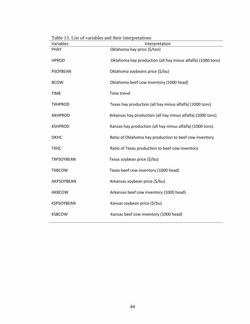
Table 13. List of variables and their interpretations
Variables Interpretation
PHAY Oklahoma hay price ($/ton)
HPROD Oklahoma hay production (all hay minus alfalfa) (1000 tons)
PSOYBEAN Oklahoma soybeans price ($/bu)
BCOW Oklahoma beef cow inventory (1000 head)
TIME Time trend
TXHPROD Texas hay production (all hay minus alfalfa) (1000 tons)
AKHPROD Arkansas hay production (all hay minus alfalfa) (1000 tons)
KSHPROD Kansas hay production (all hay minus alfalfa) (1000 tons)
OKHC Ratio of Oklahoma hay production to beef cow inventory
TXHC Ratio of Texas production to beef cow inventory
TXPSOYBEAN Texas soybean price ($/bu)
TXBCOW Texas beef cow inventory (1000 head)
AKPSOYBEAN Arkansas soybean price ($/bu)
AKBCOW Arkansas beef cow inventory (1000 head)
KSPSOYBEAN Kansas soybean price ($/bu)
KSBCOW Kansas beef cow inventory (1000 head)
VITA
KWAME ACHEAMPONG
Candidate for the Degree of
Master of Science Thesis: THE IMPACT OF SWITCHGRASS PRODUCTION ON OKLAHOMA HAY
MARKETS Major Field: Agricultural Economics
Biographical: Hail from Kumawu-Besoro in the Ashanti Region of Ghana. Born on December 27, 1975, to Mr. Kwadwo Kyei Baffour Sarkodie and Madam Antwi Khadija at Akrokere near Effiduase in the Ashanti region of Ghana.
Education: Received Teacher’s Certificate ‘A’ from Ofinso Teacher Training
College, Ofinso Ashanti, Ghana, in June 1998 and received a Bachelor of Science Agriculture from the University of Cape Coast, Cape Coast, Ghana, in June 2005. Completed the requirements for the Master of Science in Agricultural Economics at Oklahoma State University, Stillwater, Oklahoma in December 2009.
Experience: Staff at the Ministry of Education in Ghana, from September 1998 to
December 2007. Professional Memberships: Ghana National Association of Teachers.
ADVISER’S APPROVAL: Dr. Brian D. Adam
Name: Kwame Acheampong Date of Degree: December, 2009 Institution: Oklahoma State University Location: Stillwater, Oklahoma Title of Study: THE IMPACT OF SWITCHGRASS PRODUCTION ON OKLAHOMA
HAY MARKETS Pages in Study: 44 Candidate for the Degree of Master of Science
Major Field: Agricultural Economics Scope and Method of Study: Ordinary Least Square estimation was used to determine the
inverse demand function for hay in Oklahoma with price of hay as the dependent variable and time trend, hay production, price of soybean, and beef cow inventory as the independent variables. Linear Programming model was used to determine the production options between hay and switchgrass based on the economic returns of each and subject to a land constraint.
Findings and Conclusions: Oklahoma hay price is fairly stable and unresponsive to the
amount of hay produced, partly because some farmers may be producing their own hay to feed their livestock. Oklahoma hay price partly depend on the amount of hay produced in the surrounding states of Oklahoma. Finally, switchgrass production could be more profitable than hay production even at a point when switchgrass price is below the price of hay because switchgrass requires less land to produce the same unit as hay, and switchgrass has lower production cost than hay.