Supply Shocks, Demand Shocks, and Labor Market Fluctuations · PDF file · 2017-09-05Supply Shocks, Demand Shocks, and Labor Market Fluctuations ... Including aggregate hours

FEDERAL RESERVE BANK OF ST. LOUIS REVIEW MAY/JUNE 2009 155

Supply Shocks, Demand Shocks, and Labor Market Fluctuations

Helge Braun, Reinout De Bock, and Riccardo DiCecio

The authors use structural vector autoregressions to analyze the responses of worker flows, jobflows, vacancies, and hours to demand and supply shocks. They identify these shocks by restrict-ing the short-run responses of output and the price level. On the demand side, they disentangle amonetary and nonmonetary shock by restricting the response of the interest rate. The responsesof labor market variables are similar across shocks: Expansionary shocks increase job creation, thejob-finding rate, vacancies, and hours; and they decrease job destruction and the separation rate.Supply shocks have more persistent effects than demand shocks. Demand and supply shocks areequally important in driving business cycle fluctuations of labor market variables. The authors’findings for demand shocks are robust to alternative identification schemes involving the responseof labor productivity at different horizons. Supply shocks identified by restricting productivitygenerate a higher fraction of impulse responses inconsistent with standard search and matchingmodels. (JEL C32, E24, E32, J63)

Federal Reserve Bank of St. Louis Review, May/June 2009, 91(3), pp. 155-78.

to other shocks as a potential resolution (see Silvaand Toledo, 2005). These analyses are based onthe assumption that either the unconditionalmoments are driven to a large extent by a particu-lar shock or the responses of the labor market todifferent shocks are similar. This article takes astep back and asks, What are the contributions ofdifferent aggregate shocks to labor market fluc-tuations and how different are the labor marketresponses to various shocks? The labor marketvariables we analyze are worker flows, job flows,vacancies, and hours. Including both workerflows and job flows allows us to analyze thedifferent conclusions authors have reached onthe importance of the hiring versus the separa-

H all (2005) and Shimer (2004) arguethat the search and matching modelof Mortensen and Pissarides (1994)is unable to reproduce the volatility

of the job-finding rate, unemployment, and vacan-cies observed in the data.1 A growing literaturehas attempted to amend the basic Mortensen-Pissarides model to match these business cyclefacts.2 Although most of this literature considersshocks to labor productivity as the source offluctuations, some authors invoke the responses

1 Also see Andolfatto (1996).

2 See, for example, Hagedorn and Manovskii (2008) and Mortensenand Nagypál (2005).

Helge Braun is a lecturer of economics at Universität zu Köln, Reinout De Bock is an economist at the International Monetary Fund, andRiccardo DiCecio is an economist at the Federal Reserve Bank of St. Louis. The authors thank Paul Beaudry, Larry Christiano, Luca Dedola,Martin Eichenbaum, Natalia Kolesnikova, Daniel Levy, Dale Mortensen, Éva Nagypál, Frank Smets, Murat Tasci, Yi Wen, and seminar par-ticipants at the European Central Bank, Ghent University, 2006 Midwest Macroeconomics Meetings, WEAI 81st Annual Conference,University of British Columbia, and the Board of Governors for helpful comments, as well as Steven Davis and Robert Shimer for sharingtheir data. Helge Braun and Reinout De Bock thank the Research Division at the Federal Reserve Bank of St. Louis and the European CentralBank, respectively, for their hospitality. Charles Gascon provided research assistance.

© 2009, The Federal Reserve Bank of St. Louis. The views expressed in this article are those of the author(s) and do not necessarily reflect theviews of the Federal Reserve System, the Board of Governors, the regional Federal Reserve Banks, or the International Monetary Fund. Articlesmay be reprinted, reproduced, published, distributed, displayed, and transmitted in their entirety if copyright notice, author name(s), and fullcitation are included. Abstracts, synopses, and other derivative works may be made only with prior written permission of the Federal ReserveBank of St. Louis.

tion margin in driving changes in employmentand unemployment. Including aggregate hoursrelates our work to the literature on the responseof hours to technology shocks.

We identify three aggregate shocks—supplyshocks, monetary shocks, and nonmonetarydemand shocks—using a structural vector autore-gression (structural VAR, or SVAR). Restrictionsare placed on the signs of the dynamic responsesof aggregate variables as in Uhlig (2005) andPeersman (2005). The first identification schemewe consider places restrictions on the short-runresponses of output, the price level, and the inter-est rate. Supply shocks move output and the pricelevel in opposite directions, while demand shocksgenerate price and output responses of the samesign. Additionally, monetary shocks lower theinterest rate on impact; other demand shocks donot. These restrictions can be motivated by a basicIS-LM-AD-AS framework or by New Keynesianmodels. The responses of job flows, worker flows,hours, and vacancies are left unrestricted.

The main results for the labor market variablesare as follows: The responses of hours, job flows,worker flows, and vacancies are qualitativelysimilar across shocks. A positive demand or sup-ply shock increases vacancies and the job-findingand job-creation rates, and it decreases the separa-tion and job-destruction rates. As in Fujita (2004),the responses of vacancies and the job-findingrate are persistent and hump shaped. Further -more, the responses induced by demand shocksare less persistent than those induced by supplyshocks. For all shocks, changes in the job-findingrate are responsible for the bulk of changes inunemployment, although separations contributeup to one half of the change on impact. Changesin employment, on the other hand, are mostlydriven by the job-destruction rate. As in Davisand Haltiwanger (1999), we find that job reallo-cation falls after expansionary shocks, especiallydemand-side shocks. We find no evidence of dif-ferences in the matching process of unemployedworkers and vacancies in response to differentshocks. Finally, each of the demand-side shocks isat least as important as the supply-side shock inexplaining fluctuations in labor market variables.

There is mild evidence in support of a tech-nological interpretation of the supply shocks

identified by restricting output and the price level.The response of labor productivity is positive forsupply shocks at medium-term horizons, whereasit is insignificantly different from zero for demandshocks. To check the robustness of our results, wemodify the identification scheme by restrictingthe medium-run response of labor productivityto identify the supply-side shock, while leavingthe short-run responses of output and the pricelevel unrestricted. This is akin to a long-runrestriction on the response of labor productivityused in the literature (see Galì, 1999). Consistentwith the first identification scheme, technologyshocks tend to raise output and decrease the pricelevel in the short run. Labor market responses tosupply shocks under this identification schemeare less apparent. In particular, the responses ofvacancies, worker flows, and job flows to supplyshocks are not significantly different from zero.Again, the demand-side shocks are at least asimportant in explaining fluctuations in the labormarket variables as the supply shock.

We also identify a technology shock, using along-run restriction on labor productivity, and amonetary shock, by means of the recursivenessassumption used by Christiano, Eichenbaum, andEvans (1999). Again, we find that the responsesto the technology shock are not significantly dif-ferent from zero. The responses to the monetaryshock are consistent with the ones identifiedabove. The contribution of the monetary shockto the variance of labor market variables exceedsthat of the technology shock.

We also analyze the subsample stability ofour results. We find a reduction in the volatilityof shocks for the post-1984 subsample, consistentwith the Great Moderation literature. The mainconclusions from the analysis above apply to bothsubsamples.

Finally, we use a small VAR that includes onlynon-labor market variables and hours to identifythe shocks. We then uncover the responses ofthe labor market variables by regressing them ondistributed lags of the shocks.3 Our findings arerobust to this alternative empirical strategy.

Braun, De Bock, DiCecio

156 MAY/JUNE 2009 FEDERAL RESERVE BANK OF ST. LOUIS REVIEW

3 This procedure is used by Beaudry and Portier (2004) to analyzethe effects of news shocks identified in a small VAR including onlyan index of stock market value and total factor productivity onother variables of interests, such as consumption and investment.

Our results suggest that a reconciliation ofthe Mortensen-Pissarides model should equallyapply to the response of labor market variablesto demand-side shocks. Furthermore, the responseto supply-side shocks is much less clear cut thanimplicitly assumed in the bulk of the literature.In a related paper (Braun, De Bock, and DiCecio,2006) we further explore the labor marketresponses to differentiated supply shocks (seealso López-Salido and Michelacci, 2007).

Our findings suggest that the “hours debate”spawned by Galì (1999) is relevant for businesscycle models with a frictional labor market à laMortensen-Pissarides. In trying to uncover thesource of business cycle fluctuations, severalauthors have argued that a negative response ofhours worked to supply shocks is inconsistentwith the standard real business cycle (RBC) model.These results are often interpreted as suggestingthat demand-side shocks must play an importantrole in driving the cycle and are used as empiricalsupport for models that depart from the RBC stan-dard by incorporating nominal rigidities and otherfrictions. We provide empirical evidence on theresponse of job flows, worker flows, and vacan-cies. This is a necessary step to evaluate the empir-ical soundness of business cycle models with alabor market structure richer than the competitivestructure typical of the RBC models or the stylizedsticky wages structure often adopted in NewKeynesian models. The importance of demandshocks in driving labor market variables and theatypical responses to supply shocks can be inter-preted as a milder version of the “negativeresponse of hours” findings.

In the next sections, we describe the data usedin the analysis and the identification procedureand then discuss our results. The final sectioncontains the robustness analysis.

WORKER FLOWS AND JOB FLOWS DATA

Worker flows are measured by the separationand job-finding rates constructed by Shimer(2007). Their construction is summarized in the

next subsection. The following subsections dis-cuss job flows—which are measured by the job-creation and job-destruction series constructedby Faberman (2004) and Davis, Faberman, andHaltiwanger (2006)—and the business cycle statis-tics of the data.

Separation and Job-Finding Rates

The separation rate measures the rate at whichworkers leave employment and enter the unem-ployment pool. The job-finding rate measures therate at which unemployed workers exit the unem-ployment pool. Although the rates are constructedand interpreted while omitting flows betweenlabor market participation and nonparticipation,Shimer (2007) shows that they capture most of thebehavior of both the unemployment and employ-ment pools over the business cycle. The advantageof using these data lies in their availability for along time span. The data constructed by Shimerare available from 1947, whereas worker flowdata including nonparticipation flows from theCurrent Population Survey (CPS) are availableonly from 1967 onward.

The separation and job-finding rates are con-structed using data on the short-term unemploy-ment rate as a measure of separations and the lawof motion for the unemployment rate to back outa measure of the job-finding rate. The size of theunemployment pool is observed at discrete datest, t+1, t+2, etc. Hirings and separations occurcontinuously between these dates. To identifythe relevant rates within a time period, assumethat between dates t and t+1, separations and jobfinding occur with constant Poisson arrival ratesst and ft , respectively. For some τ � �0,1�, the lawof motion for the unemployment pool Ut+τ is

(1)

where Et+τ is the pool of employed workers andEt+τ st are the inflows and Ut+τ ft the outflows fromthe unemployment pool at t+τ. The analogousexpression for the pool of short-term unemployedUst+τ (i.e., those workers who have entered the

unemployment pool after date t) is:

(2)

U E s U ft t t t t+ + += −τ τ τ ,

U E s U fts

t t ts

t+ + += −τ τ τ .



Combining expressions (1) and (2) gives

(3)

Solving the differential equation using Ust = 0as the initial condition yields

Given data on Ut , Ut+1, and Ust+1, the last

expression is used to construct the job-findingrate, ft . The separation rate then follows from

(4)

where Lt � �Ut + Et� is the labor force. Notice thatthe rates st and ft are time-aggregation–adjustedversions of Us

t+1/Et+1 and �Ut – Ut+1 + Ust+1�/Ut+1,

respectively. The construction of st and ft takesinto account that workers may experience multi-ple transitions between dates t and t+1. Theserates are continuous-time arrival rates and thecorresponding probabilities are St = �1 – e–st� andFt = �1 – e–ft�, respectively.

Using equation (4), observe that if �ft + st� islarge, the unemployment rate, Ut+1/Lt, can beapproximated by the steady-state relationshiput+1 ≅ st/�st + ft�. As shown by Shimer (2007),this turns out to be an accurate approximation tothe actual unemployment rate. We use this approx-imation to infer changes in unemployment fromthe responses of ft and st in the SVAR. To gaugethe relative importance of the job-finding andseparation rates in determining unemployment,we follow Shimer (2007) and construct the follow-ing variables:

• st/�st + ft� is the approximated unemploy-ment rate;

• s–t/�s–t + ft� is the hypothetical unemploy-

ment rate computed with the actual job-finding rate, ft , and the average separationrate, s–;

• st/�st + f–� is the hypothetical unemploy-

ment rate computed with the average job-finding rate, f

–, and the actual separation

rate, st .

Inflows into the employment pool are meas-ured by the job-finding rate and not, as in Fujita

U U U U ft ts

t ts

t+ + + += − −( )τ τ τ τ .

U U e Ut tf

tst

+−

+= +1 1.

U es

f sL e Ut

f s t

t tt

f st

t t t t+

− − − −= −( ) ++1 1 ,

(2004), by the hiring rate. The hiring rate sumsall worker flows into the employment pool andscales them by current employment. Its construc-tion is analogous to the job-creation rate definedfor job flows. The response of the hiring rate toshocks is in general not very persistent, as opposedto that of the job-finding rate. This difference isdue to the scaling. We discuss this point in moredetail below.

Job Creation and Job Destruction

The job flows literature focuses on job-creation(JC) and job-destruction (JD) rates.4 Gross jobcreation sums employment gains at all plants thatexpand or start up between t–1 and t. Gross jobdestruction, on the other hand, sums up employ-ment losses at all plants that contract or shut downbetween t–1 and t. To obtain the creation anddestruction rates, both measures are divided bythe averages of employment at t–1 and t. Davis,Haltiwanger, and Schuh (1996) construct measuresfor both series from the Longitudinal ResearchDatabase (LRD) and the monthly Current Employ -ment Statistics (CES) survey from the Bureau ofLabor Statistics (BLS).5 A number of researcherswork only with the quarterly job-creation and job-destruction series from the LRD.6 Unfortunately,these series are available only for the 1972:Q1–1993:Q4 period.

This paper uses the quarterly job flows dataconstructed by Faberman (2004) and Davis,Faberman, and Haltiwanger (2006). These authorssplice together data from (i) the ManufacturingTurnover Survey (MTD) from 1947 to 1982, (ii)

4 See Davis and Haltiwanger (1992), Davis, Haltiwanger, and Schuh(1996), Davis and Haltiwanger (1999), Caballero and Hammour(2005), and López-Salido and Michelacci (2007).

5 As pointed out in Blanchard and Diamond (1990) these job-creationand -destruction measures differ from true job creation and destruc-tion as (i) they ignore gross job creation and destruction withinfirms, (ii) the point-in-time observations do not take into accountjob-creation and -destruction offsets within the quarter, and (iii)they fail to account for newly created jobs that are not yet filledwith workers.

6 Davis and Haltiwanger (1999) extend the series back to 1948. Someauthors report that this extended series is (i) somewhat less accurateand (ii) tracks only aggregate employment in the 1972:Q1–1993:Q4period (see Caballero and Hammour, 2005).



the LRD from 1972 to 1998, and (iii) the BusinessEmployment Dynamics (BED) from 1990 to 2004.The MTD and LRD data are spliced as in Davisand Haltiwanger (1999), whereas the LRD andBED splice follows Faberman (2004).

A fundamental accounting identity relates thenet employment change between any two pointsin time to the difference between job creation anddestruction. We define gE,t

JC,JD as the growth rateof employment implied by job flows:

(5)

The data spliced from the MTD and LRD ofthe job-creation and -destruction rates constructedby Davis, Faberman, and Haltiwanger (2006) per-

gE E

E EJC JDE t

JC JD t t

t tt t,

, .;−

+( ) = −−

−

1

1 2/

tain to the manufacturing sector. However, overthe period 1954:Q2–2004:Q2, the implied growthrate of employment from these job flows data,gE,tJC,JD = �JCt – JDt �, is highly correlated with the

growth rate of total nonfarm payroll employment,

7

As in Davis, Haltiwanger, and Schuh (1996),we also define gross job reallocation as rt ��JCt + JDt �. Using this definition we examine thereallocation effects of different shocks in theSVARs. We also look at cumulative reallocation.

gE E

E ECorr gE t

t t

t tE tJ

, ,: ;−

+( )

−

−

1

10 5.CC JD

E tg,,, .( ) = 0 89.



7 The correlation of gE,tJC,JD with the growth rate of employment in

manufacturing is 0.93.

Q3−54 Q4−62 Q1−71 Q2−79 Q3−87 Q4−95 Q1−04

−0.8−0.6−0.4−0.2

log(ft)

Q3−54 Q4−62 Q1−71 Q2−79 Q3−87 Q4−95 Q1−04−0.2

0

0.2

log(ft): BC Component

Q3−54 Q4−62 Q1−71 Q2−79 Q3−87 Q4−95 Q1−04

−3.5

log(st)

Q3−54 Q4−62 Q1−71 Q2−79 Q3−87 Q4−95 Q1−04

−0.05

0

0.05

log(st): BC Component

Q3−54 Q4−62 Q1−71 Q2−79 Q3−87 Q4−95 Q1−04

−3.2–3.0−2.8−2.6

log(JCt)

Q3−54 Q4−62 Q1−71 Q2−79 Q3−87 Q4−95 Q1−04

−0.1

0

0.1

log(JCt): BC Component

Q3−54 Q4−62 Q1−71 Q2−79 Q3−87 Q4−95 Q1−04

− 2.5

log(JDt)

Q3−54 Q4−62 Q1−71 Q2−79 Q3−87 Q4−95 Q1−04

−0.2

0

0.2

log(JDt): BC Component

–3.0

–3.0

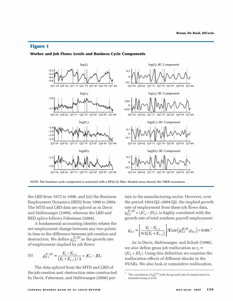
Figure 1

Worker and Job Flows: Levels and Business Cycle Components

NOTE: The business cycle component is extracted with a BP(8,32) filter. Shaded areas denote the NBER recessions.

Business Cycle Properties

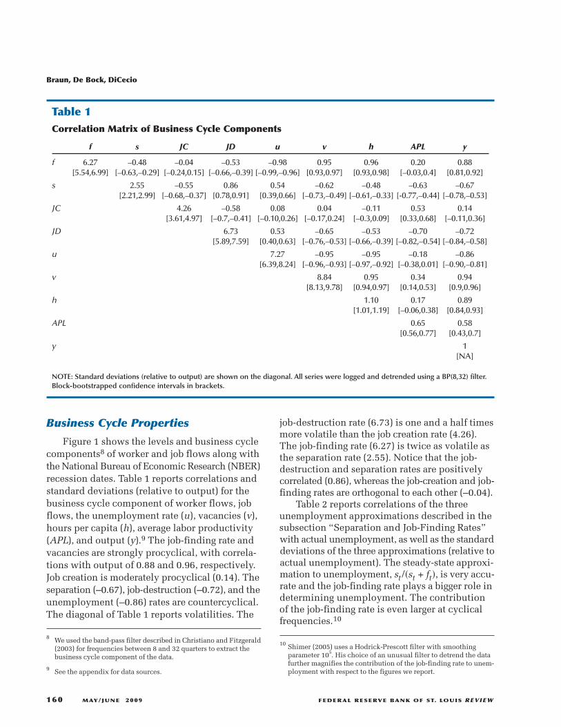
Figure 1 shows the levels and business cyclecomponents8 of worker and job flows along withthe National Bureau of Economic Research (NBER)recession dates. Table 1 reports correlations andstandard deviations (relative to output) for thebusiness cycle component of worker flows, jobflows, the unemployment rate (u), vacancies (v),hours per capita (h), average labor productivity(APL), and output (y).9 The job-finding rate andvacancies are strongly procyclical, with correla-tions with output of 0.88 and 0.96, respectively.Job creation is moderately procyclical (0.14). Theseparation (–0.67), job-destruction (–0.72), and theunemployment (–0.86) rates are countercyclical.The diagonal of Table 1 reports volatilities. The

job-destruction rate (6.73) is one and a half timesmore volatile than the job creation rate (4.26).The job-finding rate (6.27) is twice as volatile asthe separation rate (2.55). Notice that the job-destruction and separation rates are positivelycorrelated (0.86), whereas the job-creation and job-finding rates are orthogonal to each other (–0.04).

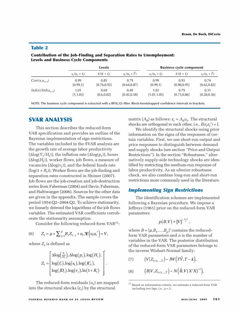
Table 2 reports correlations of the threeunemployment approximations described in thesubsection “Separation and Job-Finding Rates”with actual unemployment, as well as the standarddeviations of the three approximations (relative toactual unemployment). The steady-state approxi-mation to unemployment, st/�st + ft�, is very accu-rate and the job-finding rate plays a bigger role indetermining unemployment. The contributionof the job-finding rate is even larger at cyclicalfrequencies.10

8 We used the band-pass filter described in Christiano and Fitzgerald(2003) for frequencies between 8 and 32 quarters to extract thebusiness cycle component of the data.

9 See the appendix for data sources.



Table 1Correlation Matrix of Business Cycle Components

f s JC JD u v h APL y

f 6.27 –0.48 –0.04 –0.53 –0.98 0.95 0.96 0.20 0.88[5.54,6.99] [–0.63,–0.29] [–0.24,0.15] [–0.66,–0.39] [–0.99,–0.96] [0.93,0.97] [0.93,0.98] [–0.03,0.4] [0.81,0.92]

s 2.55 –0.55 0.86 0.54 –0.62 –0.48 –0.63 –0.67[2.21,2.99] [–0.68,–0.37] [0.78,0.91] [0.39,0.66] [–0.73,–0.49] [–0.61,–0.33] [-0.77,–0.44] [–0.78,–0.53]

JC 4.26 –0.58 0.08 0.04 –0.11 0.53 0.14[3.61,4.97] [–0.7,–0.41] [–0.10,0.26] [–0.17,0.24] [–0.3,0.09] [0.33,0.68] [–0.11,0.36]

JD 6.73 0.53 –0.65 –0.53 –0.70 –0.72[5.89,7.59] [0.40,0.63] [–0.76,–0.53] [–0.66,–0.39] [–0.82,–0.54] [–0.84,–0.58]

u 7.27 –0.95 –0.95 –0.18 –0.86[6.39,8.24] [–0.96,–0.93] [–0.97,–0.92] [–0.38,0.01] [–0.90,–0.81]

v 8.84 0.95 0.34 0.94[8.13,9.78] [0.94,0.97] [0.14,0.53] [0.9,0.96]

h 1.10 0.17 0.89[1.01,1.19] [–0.06,0.38] [0.84,0.93]

APL 0.65 0.58[0.56,0.77] [0.43,0.7]

y 1[NA]

NOTE: Standard deviations (relative to output) are shown on the diagonal. All series were logged and detrended using a BP(8,32) filter.Block-bootstrapped confidence intervals in brackets.

10 Shimer (2005) uses a Hodrick-Prescott filter with smoothingparameter 105. His choice of an unusual filter to detrend the datafurther magnifies the contribution of the job-finding rate to unem-ployment with respect to the figures we report.

SVAR ANALYSISThis section describes the reduced-form

VAR specification and provides an outline of theBayesian implementation of sign restrictions.The variables included in the SVAR analysis arethe growth rate of average labor productivity(∆log�Yt/Ht�), the inflation rate (∆log�pt�), hours(∆log�Ht�), worker flows, job flows, a measure ofvacancies (∆log�vt�), and the federal funds rate(log�1 + Rt�). Worker flows are the job-finding andseparation rates constructed in Shimer (2007).Job flows are the job-creation and job-destructionseries from Faberman (2004) and Davis, Faberman,and Haltiwanger (2006). Sources for the other dataare given in the appendix. The sample covers theperiod 1954:Q2–2004:Q2. To achieve stationarity,we linearly detrend the logarithms of the job flowsvariables. The estimated VAR coefficients corrob-orate the stationarity assumption.

Consider the following reduced-form VAR11:

(6)

where Zt is defined as

The reduced-form residuals (ut) are mappedinto the structural shocks (εt) by the structural

Z B Z u E u u Vt j

pj t j t t t= + + ′( ) =

= −∑µ1

, ,

Z

p H

f st

YH t t

t

t

t

=

( ) ( ) ( )( )

∆ ∆log , log ,log ,

log ,log tt t

t t t

JC

JD v R

( ) ( )( ) ( ) +( )

,log ,

log ,log ,ln 1

′

.

matrix (A0) as follows: εt = A0ut . The structuralshocks are orthogonal to each other, i.e., E�εtεt′� = I.

We identify the structural shocks using priorinformation on the signs of the responses of cer-tain variables. First, we use short-run output andprice responses to distinguish between demandand supply shocks (see section “Price and OutputRestrictions”). In the section “Robustness,” alter-natively supply-side technology shocks are iden-tified by restricting the medium-run response oflabor productivity. As an ulterior robustnesscheck, we also combine long-run and short-runrestrictions more commonly used in the literature.

Implementing Sign Restrictions

The identification schemes are implementedfollowing a Bayesian procedure. We impose aJeffreys (1961) prior on the reduced-form VARparameters:

where B = [µ,B1,…,Bp]′ contains the reduced-form VAR parameters and n is the number ofvariables in the VAR. The posterior distributionof the reduced-form VAR parameters belongs tothe inverse Wishart-Normal family:

(7)

(8)

p B V Vn

, ,( ) − +

~1

2

V Z IW TV T kt T= …( ) −( )1, , , ,~ ˆ

B V Z N B V X Xt T, , ,, ,=−( ) ′( )( )1

1... ~ ˆ



11 Based on information criteria, we estimate a reduced-form VARincluding two lags, i.e., p = 2.

Table 2Contribution of the Job-Finding and Separation Rates to Unemployment:Levels and Business Cycle Components

Levels Business cycle component

st/(st + ft) s–/(s– + ft) st/(st + f–) st/(st + ft) s–/(s– + ft) st/(st + f

–)

Corr(x,ut+1) 0.99 0.85 0.79 0.99 0.93 0.74[0.99,1] [0.76,0.92] [0.64,0.87] [0.99,1] [0.90,0.95] [0.62,0.82]

Std(x)/Std(ut+1) 1.01 0.69 0.49 1.03 0.79 0.31[1,1.03] [0.6,0.82] [0.42,0.58] [1.01,1.05] [0.73,0.86] [0.28,0.36]

NOTE: The business cycle component is extracted with a BP(8,32) filter. Block-bootstrapped confidence intervals in brackets.

where B̂ and V̂ are the ordinary least squaresestimates of B and V,T, is the sample length, k = �np + 1�, and X is defined as

Consider a possible orthogonal decompositionof the covariance matrix, i.e., a matrix C such thatV = CC ′. Then CQ, where Q is a rotation matrix,is also an admissible decomposition. The posteriordistribution on the reduced-form VAR parameters,a uniform distribution over rotation matrices, andan indicator function equal to zero on the set ofimpulse response functions (IRFs) that violatethe identification restrictions induce a posteriordistribution over the IRFs that satisfy the signrestrictions.

The sign restrictions are implemented asfollows:

1. For each draw from the inverse Wishart-Normal family for �V,B�, we take an orthog-onal decomposition matrix, C, and drawone possible rotation, Q.12

2. We check the signs of the impulse responsesfor each structural shock. If we find a setof structural shocks that satisfies the restric-tions, we keep the draw. Otherwise wediscard it.

3. We continue until we have 1,000 drawsfrom the posterior distribution of the IRFsthat satisfy the identifying restrictions.

X x x

x Z Z

T

t t t p

= ′ ′[ ]′

′ = ′ ′ ′

− −

1

11

, , ,

, , ,

...

... ..

PRICE AND OUTPUTRESTRICTIONS

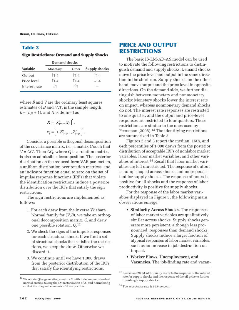
The basic IS-LM-AD-AS model can be usedto motivate the following restrictions to distin-guish demand and supply shocks. Demand shocksmove the price level and output in the same direc-tion in the short run. Supply shocks, on the otherhand, move output and the price level in oppositedirections. On the demand side, we further dis-tinguish between monetary and nonmonetaryshocks: Monetary shocks lower the interest rateon impact, whereas nonmonetary demand shocksdo not. The interest rate responses are restrictedto one quarter, and the output and price-levelresponses are restricted to four quarters. Theserestrictions are similar to the ones used byPeersman (2005).13 The identifying restrictionsare summarized in Table 3.

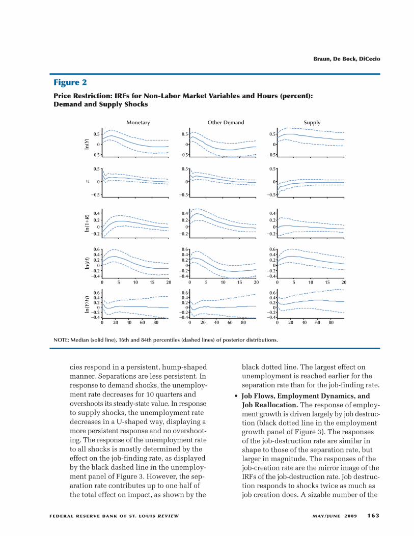
Figures 2 and 3 report the median, 16th, and84th percentiles of 1,000 draws from the posteriordistribution of acceptable IRFs of nonlabor marketvariables, labor market variables, and other vari-ables of interest.14 Recall that labor market vari-ables are left unrestricted. The response of outputis hump shaped across shocks and more persis -tent for supply shocks. The response of hours ispositive for all shocks and the response of laborproductivity is positive for supply shocks.

For the response of the labor market vari-ables displayed in Figure 3, the following mainobservations emerge:

• Similarity Across Shocks. The responsesof labor market variables are qualitativelysimilar across shocks. Supply shocks gen-erate more persistent, although less pro-nounced, responses than demand shocks.Supply shocks induce a larger fraction ofatypical responses of labor market variables,such as an increase in job destruction onimpact.

• Worker Flows, Unemployment, andVacancies. The job-finding rate and vacan-

12 We obtain Q by generating a matrix X with independent standardnormal entries, taking the QR factorization of X, and normalizingso that the diagonal elements of R are positive.



Table 3Sign Restrictions: Demand and Supply Shocks

Demand shocks

Variable Monetary Other Supply shocks

Output ↑1-4 ↑1-4 ↑1-4Price level ↑1-4 ↑1-4 ↓1-4Interest rate ↓1 ↑1 —

13 Peersman (2005) additionally restricts the response of the interestrate for supply shocks and the response of the oil price to furtherdisentangle supply shocks.

14 The acceptance rate is 66.6 percent.

cies respond in a persistent, hump-shapedmanner. Separations are less persistent. Inresponse to demand shocks, the unemploy-ment rate decreases for 10 quarters andovershoots its steady-state value. In responseto supply shocks, the unemployment ratedecreases in a U-shaped way, displaying amore persistent response and no overshoot-ing. The response of the unemployment rateto all shocks is mostly determined by theeffect on the job-finding rate, as displayedby the black dashed line in the unemploy-ment panel of Figure 3. However, the sep-aration rate contributes up to one half ofthe total effect on impact, as shown by the

black dotted line. The largest effect onunemployment is reached earlier for theseparation rate than for the job-finding rate.

• Job Flows, Employment Dynamics, andJob Reallocation. The response of employ-ment growth is driven largely by job destruc-tion (black dotted line in the employmentgrowth panel of Figure 3). The responsesof the job-destruction rate are similar inshape to those of the separation rate, butlarger in magnitude. The responses of thejob-creation rate are the mirror image of theIRFs of the job-destruction rate. Job destruc-tion responds to shocks twice as much asjob creation does. A sizable number of the



−0.5

0

0.5

Monetary

−0.5

0

0.5

Other Demand

−0.5

0

0.5

Supply

−0.5

0

0.5

−0.5

0

0.5

−0.5

0

0.5

−0.20

0.20.4

−0.20

0.20.4

−0.20

0.20.4

0 5 10 15 20−0.4−0.2

00.20.40.6

0 5 10 15 20−0.4−0.2

00.20.40.6

0 5 10 15 20−0.4−0.2

00.20.40.6

0 20 40 60 80−0.4−0.2

00.20.40.6

0 20 40 60 80−0.4−0.2

00.20.40.6

0 20 40 60 80−0.4−0.2

00.20.40.6

ln(Y

)ln

(1+

R)

ln(H

)ln

(Y/H

)π

Figure 2

Price Restriction: IRFs for Non-Labor Market Variables and Hours (percent): Demand and Supply Shocks

NOTE: Median (solid line), 16th and 84th percentiles (dashed lines) of posterior distributions.

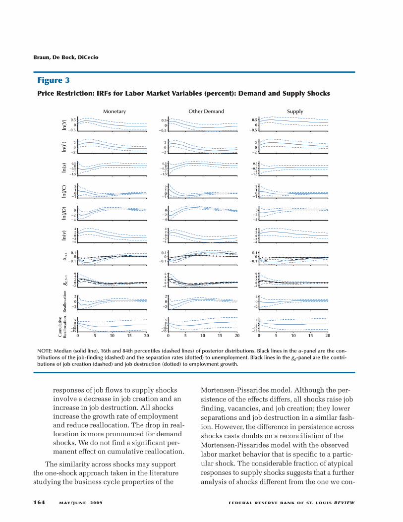
responses of job flows to supply shocksinvolve a decrease in job creation and anincrease in job destruction. All shocksincrease the growth rate of employmentand reduce reallocation. The drop in real-location is more pronounced for demandshocks. We do not find a significant per-manent effect on cumulative reallocation.

The similarity across shocks may supportthe one-shock approach taken in the literaturestudying the business cycle properties of the

Mortensen-Pissarides model. Although the per-sistence of the effects differs, all shocks raise jobfinding, vacancies, and job creation; they lowerseparations and job destruction in a similar fash-ion. However, the difference in persistence acrossshocks casts doubts on a reconciliation of theMortensen-Pissarides model with the observedlabor market behavior that is specific to a partic-ular shock. The considerable fraction of atypicalresponses to supply shocks suggests that a furtheranalysis of shocks different from the one we con-



−0.50

0.5

Monetary Other Demand Supply

−202

−202

−202

−1.5−1

−0.50

0.5

−1012

−1012

−1012

−4−2

0

−4−2

0

−4−2

0

−4−2

024

−0.10

0.1

–20246

−202

−202

−202

0 5 10 15 20–15–10–5

05

0 5 10 15 20 0 5 10 15 20

ln(Y

)u t

+1

−0.50

0.5

−0.50

0.5

−1.5−1

−0.50

0.5

−1.5−1

−0.50

0.5

−4−2

024

−4−2

024

−0.10

0.1

−0.10

0.1

0246

0246

–15–10–5

05

–15–10–5

05

ln(f

)ln

(s)

ln(J

C)

ln(J

D)

ln(v

)g E

,t+

1

–2 –2

Rea

lloca

tio

nC

umul

ativ

eR

eallo

cati

on

Figure 3

Price Restriction: IRFs for Labor Market Variables (percent): Demand and Supply Shocks

NOTE: Median (solid line), 16th and 84th percentiles (dashed lines) of posterior distributions. Black lines in the u-panel are the con-tributions of the job-finding (dashed) and the separation rates (dotted) to unemployment. Black lines in the gE-panel are the contri-butions of job creation (dashed) and job destruction (dotted) to employment growth.

sider is necessary (see Braun, De Bock, and DiCecio,2006; López-Salido and Michelacci, 2007).

The hump-shaped response of the job-findingrate and vacancies to shocks is not consistent withthe Mortensen-Pissarides model and with most ofthe literature. This finding is in line with Fujita(2004), who identifies a unique aggregate shockin a trivariate VAR including worker flows vari-ables, scaled by employment, and vacancies. Thisaggregate shock is identified by restricting theresponses of employment growth (nonnegativefor four quarters), the separation rate (nonpositiveon impact), and the hiring rate (nonnegative onimpact). Our identification strategy confirms thesefindings without restricting worker flow variables.Where we use the job-finding probability in ourVAR, Fujita (2004) includes the hiring rate tomeasure worker flows into employment. The hir-ing rate measures worker flows into employmentscaled by the size of the employment pool. Thejob-finding rate measures the probability of exitingthe unemployment pool. Although both arguablyreflect movements of workers into employment(see Shimer, 2007), the difference in scaling leadsto a different qualitative behavior of the two seriesin response to an aggregate shock. The responseof the job-finding rate shows a persistent increase.Fujita’s hiring rate initially increases but quicklydrops below zero because of the swelling employ-ment pool.

The mildly negative effect on cumulativereallocation is at odds with Caballero andHammour (2005), who find that expansionaryaggregate shocks have positive effects on cumu-lative reallocation.

For monetary policy shocks, the IRFs of aggre-gate variables are consistent with Christiano,Eichenbaum, and Evans (1999), who use a recur-siveness restriction to identify a monetary policyshock. However, Christiano, Eichenbaum, andEvans (1999) obtain a more persistent interest rateresponse and inflation exhibits a price puzzle,i.e., inflation declines in response to an expan-sionary monetary policy shock. The latter differ-ence is forced by our identification scheme. Thejob flows responses are consistent with estimatesin Trigari (2009) and the worker flows and vacan-cies responses with those in Braun (2005).

The last row of Figure 2 shows the IRFs oflabor productivity for 100 quarters. Average laborproductivity, which is unrestricted, displays apersistent yet weak increase in response to supplyshocks. On the other hand, productivity showsno persistent response to demand or monetaryshocks. The medium-run response of labor pro-ductivity to supply shocks is consistent with atechnology shocks interpretation.

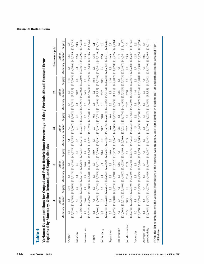
Table 4 reports the median of the posteriordistribution of variance decompositions, i.e., thepercentage of the j-periods-ahead forecast erroraccounted for by the identified shocks. The fore-cast errors of output and labor productivity aredriven primarily by supply shocks. Interestingly,the demand shocks have a greater impact on labormarket variables than the supply shock. Thegreater importance of demand shocks suggeststhat more attention should be paid to shocks otherthan technology in the evaluation of the basiclabor market search model.

A vast and growing literature analyzes theresponse of hours worked to technology shocksin VARs. Shea (1999), Galì (1999, 2004), Basu,Fernald, and Kimball (2006), and Francis andRamey (2005) argue that hours decrease on impactin response to technology shocks. This result isat odds with the standard RBC model, whichimplies an increase in hours worked in responseto a positive technology shock. The conclusiondrawn is that the RBC model should be amendedby including nominal rigidities, habit formationin consumption and investment adjustment costs,a short-run fixed proportion technology, or differ-ent shocks.15 Our results on the importance ofdemand shocks in driving labor market variablesand on atypical responses of these variables tosupply shocks can be interpreted as an extensionof the negative hours response findings, thoughin a milder form.

The last column in Table 4 shows the variancecontributions of the shocks at business cycle fre-quencies. The contribution of shock i to the totalvariance is computed as follows:



15 Christiano, Eichenbaum, and Vigufsson (2004), on the other hand,argue that the negative impact response of hours to technologyshocks is an artifact of overdifferencing hours in VARs.



Table 4

Variance Decompositions for Output and Price Restrictions: Percentage of the j-Periods-Ahead Forecast Error

Explained by Monetary, Other Dem

and, and Supply Shocks

48

2032

Busines

s cy

cle

Other

Other

Other

Other

Other

Monetary

dem

and

Supply

Monetary

dem

and

Supply

Monetary

dem

and

Supply

Monetary

dem

and

Supply

Monetary

dem

and

Supply

Output

9.5

6.4

13.4

8.1

5.8

14.4

7.1

7.0

12.3

6.7

6.9

11.5

9.3

12.5

9.8

[2.7,23.8][1.6,19.9][3.8,30.9][2.5,21.3][2.4,13.4][4.4,32.5][2.8,15.5][2.5,16.7][3.9,28.2][2.8,15.1][2.7,6.9][3.7,26.3][3.4,20.6][4.3,25.9][2.9,23.5]

Inflation

6.8

8.6

9.5

8.4

9.6

8.5

8.7

9.6

9.0

9.1

10.2

9.3

6.1

12.4

10.3

[2.1,18.6][2.4,24.8][2.3,27.8][2.5,21.3][2.8,26.4][2.4,23.7][2.9,21.5][3.7,23.4][3.3,21.3][3.4,19.7][4.2,10.2][3.7,20.9][1.7,16.1][4.3,29.5][3.4,25.2]

Interest rate

4.8

19.6

5.2

6.9

20.0

5.4

7.7

17.7

7.0

8.0

16.3

8.0

6.5

15.5

5.8

[1.6,11.7][5.4,29.6][1.3,18.3][2.4,14.8][6.4,38.4][1.6,14.9][3.0,17.1][6.9,32.3][2.5,15.0][3.3,16.4][6.9,16.3][3.3,15.7][2.3,14.3][4.7,33.6][1.6,14.4]

Hours

8.4

7.8

8.5

8.9

6.0

10.9

8.6

9.0

10.8

9.1

9.2

10.4

9.3

13.8

9.1

[1.2,26.6][1.4,26.5][1.4,27.4][1.8,25.5][1.9,17.1][2.2,29.8][2.8,19.2][3.0,19.2][3.2,25.1][3.1,18.9][3.5,9.2][3.8,22.8][2.6,24.1][4.0,31.6][2.6,23.1]

Job finding

9.3

6.8

8.2

9.4

6.1

10.4

8.5

10.7

10.0

8.6

11.2

10.1

9.5

12.8

9.2

[2.0,27.8][1.7,22.8][2.2,25.7][1.9,26.3][2.2,16.0][2.5,28.7][2.7,18.7][4.1,21.6][3.2,25.4][3.1,18.6][4.4,11.2][3.5,23.8][2.6,24.3][3.5,31.1][2.8,22.5]

Separation

8.7

6.3

8.8

8.5

8.5

10.0

8.8

10.0

10.8

8.6

9.5

11.0

9.3

10.9

8.7

[2.7,22.5][1.7,18.0][2.4,22.3][3.2,19.8][3.3,17.7][3.3,21.9][3.8,16.7][4.2,18.5][4.0,21.1][3.8,15.3][4.3,9.5][4.4,20.7][3.6,22.0][3.4,27.6][2.7,29.8]

Job creation

7.2

9.7

7.2

8.6

12.6

7.8

9.6

12.5

8.4

9.6

12.5

8.4

7.3

11.4

6.2

[2.1,20.9][3.5,21.7][2.5,19.0][3.4,18.7][5.4,22.8][3.1,18.0][4.3,20.0][5.7,22.1][3.6,17.4][4.4,19.5][5.7,12.5][3.7,17.3][2.3,18.7][4.4,24.1][1.8,15.7]

Job destruction

11.5

10.3

6.6

11.4

11.9

7.5

11.3

12.7

7.5

11.2

12.8

7.7

9.5

13.3

6.3

[3.8,27.8][2.7,26.1][2.2,17.9][4.1,24.9][4.1,24.8][3.0,17.5][4.4,25.3][4.9,25.3][3.1,16.5][4.4,24.9][5.1,12.8][3.2,16.1][2.9,22.8][3.6,28.7][1.8,16.3]

Vacancies

9.0

5.5

7.9

8.5

6.3

9.3

9.0

11.5

8.6

9.3

11.4

8.8

9.7

12.5

8.6

[1.0,27.0][1.1,19.4][1.1,25.9][1.4,25.5][2.5,14.6][1.6,27.8][3.0,18.3][4.3,24.3][2.5,22.0][3.3,18.7][4.7,11.4][3.3,20.8][2.3,23.0][3.9,27.4][2.3,22.0]

Average labor

4.4

4.8

7.7

4.6

5.7

7.4

4.5

5.4

6.6

4.5

5.5

7.4

7.5

10.5

8.8

productivity

[1.0,16.5][1.4,15.7][1.4,27.9][1.4,14.9][1.6,16.6][1.6,24.7][1.3,14.3][1.5,17.0][1.6,22.7][1.3,14.5][1.5,5.5][1.7,24.2] [2.8,17.0][3.6,20.8][2.6,21.1]

NOTE: The last column presents the variance contributions at the business cycle frequency (see text). N

umbers in brackets are 16th and 84th percentiles obtained from

1,000 draws.

• We simulate data with only shock i, say Zti.

• We band-pass filter Zti and Zt to obtain their

business cycle components, �Zti�BC and

�Zt�BC, respectively.

• The contribution of shock i is computedby dividing the variance of �Zt

i�BC by thevariance of �Zt�

BC.

The three right panels of Table 4 show the vari-ance contribution with the price-output restriction.The nonmonetary demand shock is the mostimportant shock. The monetary and supply shockscontribute about equally to the business cyclevariation of labor and non-labor market variables.

Matching Function Estimates

We investigate further the possibility of differ-ential labor market responses to shocks by esti-mating a shock-specific matching function. In theMortensen-Pissarides model, the number of hires�f × U � is related to the size of the unemploymentpool and the number of vacancies via a matchingfunction, M�U,V �.16 Assuming a Cobb-Douglasfunctional form, the matching function is given by

(9)

where αv is the elasticity of the number of matcheswith respect to vacancies, αu is the elasticity withrespect to unemployment, and A captures theoverall efficiency of the matching process.

Under the assumption of constant returns toscale (CRS), i.e., αu + αv =1, the job-finding ratecan then be expressed as

(10)

If we do not impose CRS, then

(11)

To consider the effect of the shocks identifiedabove on the matching process, we obtain a sam-ple of 1,000 draws from the posterior distributionsof A and the elasticity parameters estimated fromartificial data. Each draw involves the followingsteps:

• a vector of accepted residuals is constructedas if the shock(s) of interest were the onlystructural shock(s);

• this vector of accepted residuals and theVAR parameters are used to generate arti-ficial data, Z~t;

M U V AU Vu v, ,( ) = α α

log log log log .f A v ut v t t( ) = ( ) + ( ) − ( )( )α

log log log log .f A v ut v t u t( ) = ( ) + ( ) − ( )α α



16 Petrongolo and Pissarides (2001) survey the matching functionliterature.

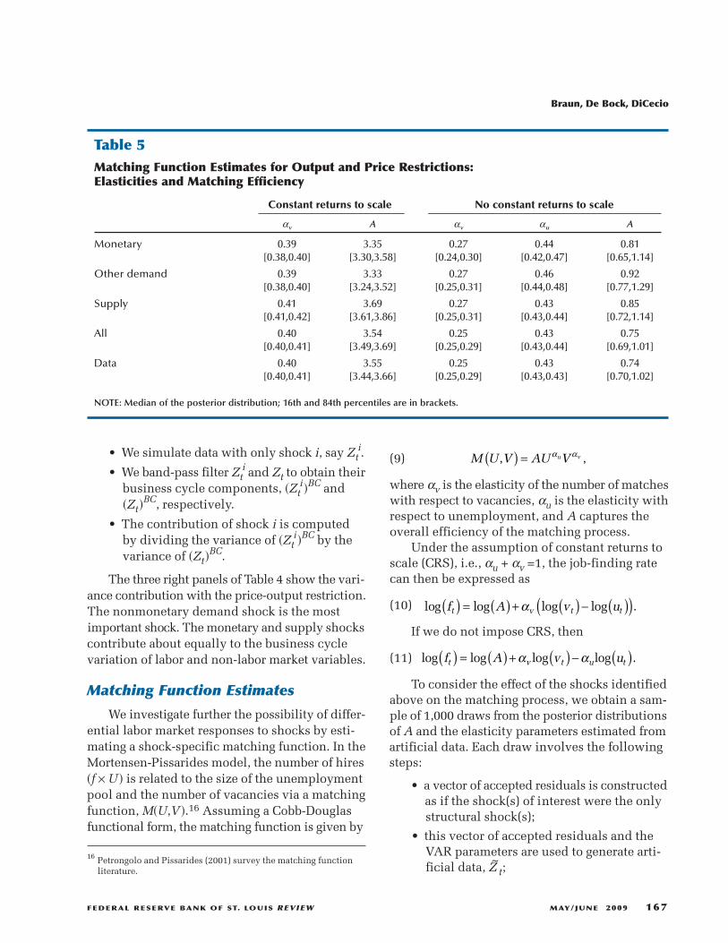
Table 5Matching Function Estimates for Output and Price Restrictions:Elasticities and Matching Efficiency

Constant returns to scale No constant returns to scale

αv A αv αu A

Monetary 0.39 3.35 0.27 0.44 0.81[0.38,0.40] [3.30,3.58] [0.24,0.30] [0.42,0.47] [0.65,1.14]

Other demand 0.39 3.33 0.27 0.46 0.92[0.38,0.40] [3.24,3.52] [0.25,0.31] [0.44,0.48] [0.77,1.29]

Supply 0.41 3.69 0.27 0.43 0.85[0.41,0.42] [3.61,3.86] [0.25,0.31] [0.43,0.44] [0.72,1.14]

All 0.40 3.54 0.25 0.43 0.75[0.40,0.41] [3.49,3.69] [0.25,0.29] [0.43,0.44] [0.69,1.01]

Data 0.40 3.55 0.25 0.43 0.74[0.40,0.41] [3.44,3.66] [0.25,0.29] [0.43,0.43] [0.70,1.02]

NOTE: Median of the posterior distribution; 16th and 84th percentiles are in brackets.

• unemployment is constructed using thesteady-state approximation u~t+1 ≅ s~t/�s

~t +

f~t� from the artificial data;

• log�f~t� is regressed on either log�v~t� and

log�u~t� (not assuming CRS) or log�v~t/u~t�

(under the CRS assumption).

The artificial data constructed using onlymonetary shocks, for example, induce a posteriordistribution for the elasticity parameters and Afor a hypothetical economy in which monetaryshocks are the only source of fluctuations.

Table 5 reports the median, 16th, and 84thpercentiles of 1,000 draws from the posteriordistributions for the price-output identificationscheme. The first two columns show the estimatesfor αv and A when CRS are imposed. The CRSestimates suggest that aggregate shocks do notentail a differential effect on the matching process.The estimated efficiency parameters are somewhatlower for monetary and demand shocks than forthe supply shock, but the median estimates differby less than 5 percent. The last three columns ofTable 5 show the unrestricted estimates for αv, αu ,and A. Estimates of αv and αu across shocks areclose and the sum of the coefficients is around0.70, corresponding to decreasing returns to scale.There are no significant differences in the medianestimates of the efficiency parameter A.

ROBUSTNESSWe analyze the robustness of our results by

considering medium-run and long-run restrictionson productivity to identify technology shocks.

Subsample stability and a minimal VAR specifi-cation to identify the shocks of interest are alsoconsidered.

Restricting the Medium-Run Responseof Labor Productivity

Pushing the technological interpretationfurther, we identify supply shocks as ones thatincrease labor productivity in the medium run.The short-run responses of output and the pricelevel are left unrestricted. This allows us to cap-ture, as supply shocks, news effects on future tech-nological improvements (see Beaudry and Portier,2006). Also, this restriction is similar to the long-run restrictions used in the literature (see Galì,1999). We will analyze the latter in the next sub-section. The advantage of a medium-run restrictionis that it allows the identification of the othershocks within the same framework as above.

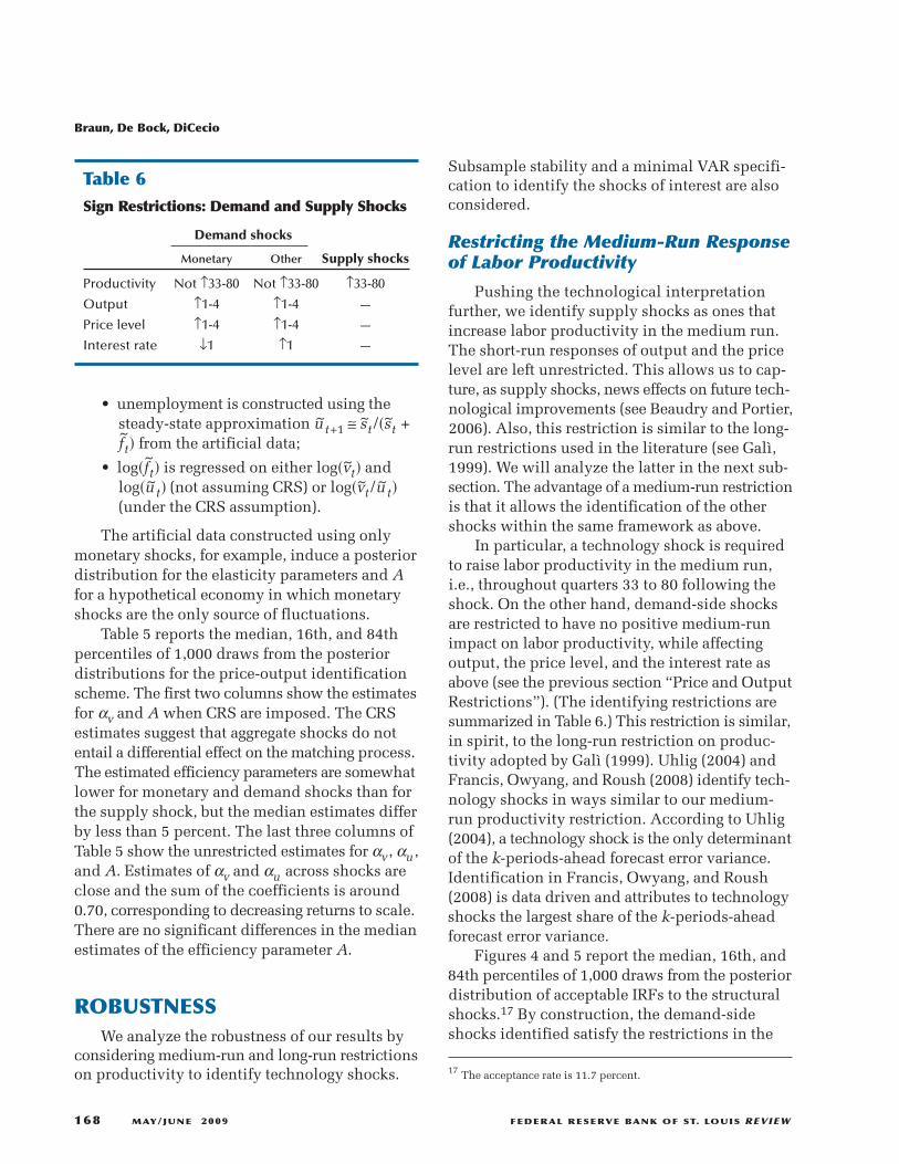
In particular, a technology shock is requiredto raise labor productivity in the medium run,i.e., throughout quarters 33 to 80 following theshock. On the other hand, demand-side shocksare restricted to have no positive medium-runimpact on labor productivity, while affectingoutput, the price level, and the interest rate asabove (see the previous section “Price and OutputRestrictions”). (The identifying restrictions aresummarized in Table 6.) This restriction is similar,in spirit, to the long-run restriction on produc-tivity adopted by Galì (1999). Uhlig (2004) andFrancis, Owyang, and Roush (2008) identify tech-nology shocks in ways similar to our medium-run productivity restriction. According to Uhlig(2004), a technology shock is the only determinantof the k-periods-ahead forecast error variance.Identification in Francis, Owyang, and Roush(2008) is data driven and attributes to technologyshocks the largest share of the k-periods-aheadforecast error variance.

Figures 4 and 5 report the median, 16th, and84th percentiles of 1,000 draws from the posteriordistribution of acceptable IRFs to the structuralshocks.17 By construction, the demand-sideshocks identified satisfy the restrictions in the

17 The acceptance rate is 11.7 percent.



Table 6Sign Restrictions: Demand and Supply Shocks

Demand shocks

Monetary Other Supply shocks

Productivity Not ↑33-80 Not ↑33-80 ↑33-80Output ↑1-4 ↑1-4 —

Price level ↑1-4 ↑1-4 —

Interest rate ↓1 ↑1 —

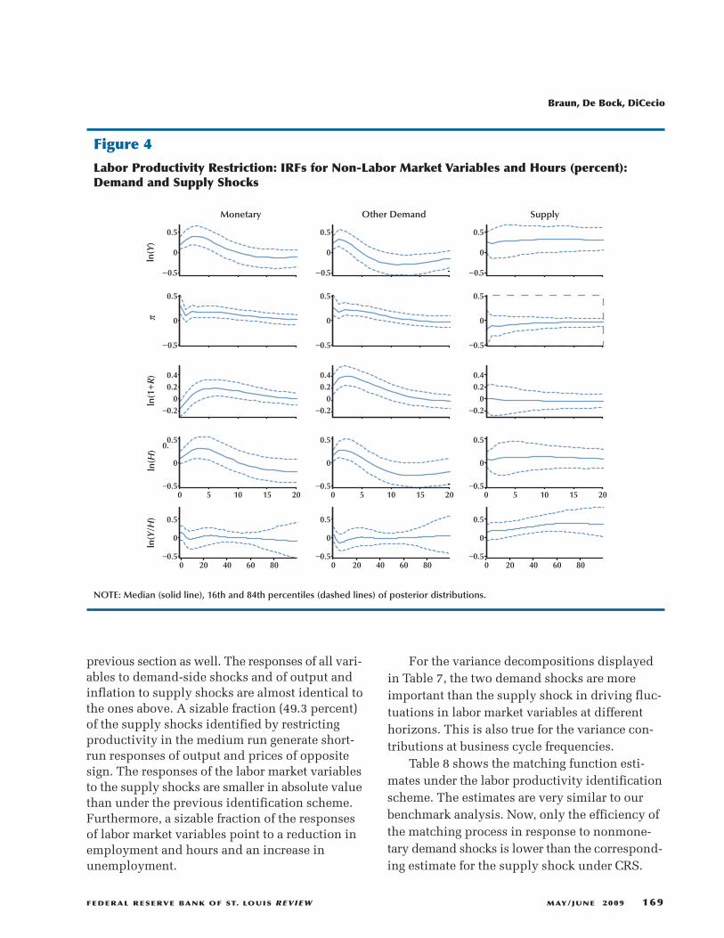
previous section as well. The responses of all vari-ables to demand-side shocks and of output andinflation to supply shocks are almost identical tothe ones above. A sizable fraction (49.3 percent)of the supply shocks identified by restrictingproductivity in the medium run generate short-run responses of output and prices of oppositesign. The responses of the labor market variablesto the supply shocks are smaller in absolute valuethan under the previous identification scheme.Furthermore, a sizable fraction of the responsesof labor market variables point to a reduction inemployment and hours and an increase inunemployment.

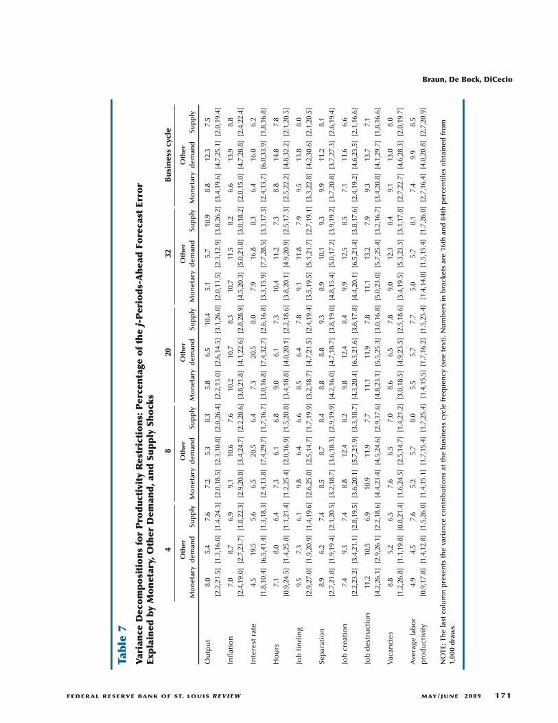
For the variance decompositions displayedin Table 7, the two demand shocks are moreimportant than the supply shock in driving fluc-tuations in labor market variables at differenthorizons. This is also true for the variance con-tributions at business cycle frequencies.

Table 8 shows the matching function esti-mates under the labor productivity identificationscheme. The estimates are very similar to ourbenchmark analysis. Now, only the efficiency ofthe matching process in response to nonmone-tary demand shocks is lower than the correspond -ing estimate for the supply shock under CRS.



−0.5

0

0.5

−0.5

0

0.5

−0.5

0

0.5

−0.5

0

0.5

−0.5

0

0.5

−0.5

0

0.5

−0.20

0.20.4

−0.20

0.20.4

−0.20

0.20.4

−0.5

0

0.5

−0.5

0

0.5

−0.5

0

0.5

−0.5

0

0.5

−0.5

0

0.5

−0.5

0

0.5

0 20 40 60 80 0 20 40 60 80 0 20 40 60 80

0 5 10 15 20 0 5 10 15 20 0 5 10 15 20


0.

ln(Y

)ln

(1+

R)

ln(H

)ln

(Y/H

)π

Figure 4

Labor Productivity Restriction: IRFs for Non-Labor Market Variables and Hours (percent): Demand and Supply Shocks

NOTE: Median (solid line), 16th and 84th percentiles (dashed lines) of posterior distributions.



−0.50

0.5

−202

−101

−1012

−4−2

02

−4−2

024

−0.10

0.1

− 20246

−202

−100

10

0 5 10 15 20 0 5 10 15 20 0 5 10 15 20

−0.50

0.5

−0.50

0.5

−202

−202

−101

−101

−1012

−1012

−4−2

02

−4−2

02

−4−2

024

−4−2

024

−0.10

0.1

−0.10

0.1

− 20246

− 20246

−202

−202

−100

10

−100

10


ln

(Y)

u t+

1ln

(f )

ln(s

)ln

(JC

)ln

(JD

)ln

(v)

g E,t

+1

Rea

lloca

tio

nC

umul

ativ

eR

eallo

cati

on

Figure 5

Labor Productivity Restriction: IRFs for Labor Market Variables (percent): Demand and Supply Shocks

NOTE: Median (solid line), 16th and 84th percentiles (dashed lines) of posterior distributions. Black lines in the u-panel are the con-tributions of the job-finding (dashed) and the separation rates (dotted) to unemployment. Black lines in the gE-panel are the contri-butions of job creation (dashed) and job destruction (dotted) to employment growth.



Table 7

Variance Decompositions for Productivity Restrictions: Percentage of the j-Periods-Ahead Forecast Error

Explained by Monetary, Other Dem

and, and Supply Shocks

48

2032

Busines

s cy

cle

Other

Other

Other

Other

Other

Monetary

dem

and

Supply

Monetary

dem

and

Supply

Monetary

dem

and

Supply

Monetary

dem

and

Supply

Monetary

dem

and

Supply

Output

8.0

5.4

7.6

7.2

5.3

8.3

5.8

6.5

10.4

5.1

5.7

10.9

8.8

12.3

7.5

[2.2,21.5][1.3,16.0][1.4,24.3][2.0,18.5][2.3,10.8][2.0,26.4][2.2,13.0][2.6,14.5][3.1,26.0][2.0,11.5][2.3,12.9][3.8,26.2][3.4,19.6][4.7,25.1][2.0,19.4]

Inflation

7.0

8.7

6.9

9.1

10.6

7.6

10.2

10.7

8.3

10.7

11.5

8.2

6.6

13.9

8.8

[2.4,19.0][2.7,23.7][1.8,22.3][2.9,20.8][ 3.4,24.7][2.2,20.6][3.8,21.8][4.1,22.6][2.8,28.9][4.5,20.3][5.0,21.8][3.0,18.2][2.0,15.0][4.7,28.8][2.4,22.4]

Interest rate

4.5

19.5

5.6

6.5

20.5

6.4

7.3

20.5

8.0

7.9

16.8

8.3

6.4

16.0

6.2

[1.8,10.4][6.5,41.4][1.3,18.3][2.4,13.8][7.4,29.7][1.7,16.7][3.0,16.8][7.4,32.7][2.6,16.8][3.3,15.9][7.7,28.5][3.1,17.3][2.4,13.7][6.0,33.9][1.8,16.8]

Hours

7.1

8.0

6.4

7.3

6.1

6.8

9.0

6.1

7.3

10.4

11.2

7.3

8.8

14.8

7.8

[0.9,24.5][1.4,25.8][1.1,21.4][1.2,25.4][2.0,16.9][1.5,20.8][3.4,18.8][4.0,20.1][2.2,18.6][3.8,20.1][4.9,20.9][2.5,17.3][2.5,22.2][4.8,32.2][2.1,20.5]

Job finding

9.5

7.3

6.1

9.8

6.4

6.6

8.5

6.4

7.8

9.1

11.8

7.9

9.5

13.8

8.0

[2.9,27.0][1.9,20.9][1.4,19.6][2.6,25.0][2.5,14.7][1.7,19.9][3.2,18.7][4.7,21.5][2.4,19.4][3.5,19.5][5.1,21.7][2.7,19.1][3.3,22.8][4.2,30.6][2.1,20.5]

Separation

8.9

6.2

7.4

8.5

8.7

8.4

8.8

8.8

9.3

8.9

10.1

9.3

9.9

11.2

8.1

[2.7,21.8][1.9,19.4][2.1,20.5][3.2,18.7][3.6,18.3][2.9,19.9][4.2,16.0][4.7,18.7][3.8,19.0][4.8,15.4][5.0,17.2][3.9,19.2][3.7,20.8][3.7,27.3][2.6,19.4]

Job creation

7.4

9.3

7.4

8.8

12.4

8.2

9.8

12.4

8.4

9.9

12.5

8.5

7.1

11.6

6.6

[2.2,23.2][3.4,21.1][2.8,19.5][3.6,20.1][5.7,21.9][3.3,18.7][4.3,20.4][6.3,21.6][3.6,17.8][4.4,20.1][6.5,21.4][3.8,17.6][2.4,19.2][4.6,23.5][2.1,16.6]

Job destruction

11.2

10.5

6.9

10.9

11.9

7.7

11.1

11.9

7.8

11.1

13.2

7.9

9.3

13.7

7.1

[4.2,26.1][2.9,26.1][2.2,18.6][4.4,23.4][4.5,24.6][2.9,17.6][4.8,23.1][5.5,25.3][3.0,16.8][5.0,23.0][5.7,25.4][3.2,16.7][3.4,20.8][4.1,29.7][1.8,16.6]

Vacancies

8.8

5.2

6.5

7.6

6.5

7.0

8.6

6.5

7.8

9.0

12.3

8.4

9.1

13.0

8.0

[1.2,26.8][1.1,19.8][0.8,21.4][1.6,24.5][2.5,14.7][1.4,21.2][3.0,18.5][4.9,23.5][2.5,18.6][3.4,19.5][5.3,23.3][3.1,17.8][2.7,22.7][4.6,28.3][2.0,19.7]

Average labor

4.9

4.5

7.6

5.2

5.7

8.0

5.5

5.7

7.7

5.0

5.7

8.1

7.4

9.9

8.5

productivity

[0.9,17.8][1.4,12.8][1.5,26.0][1.4,15.1][1.7,15.4][1.7,25.4][1.4,15.5][1.7,16.2][1.5,25.4][1.4,14.0][1.5,15.4][1.7,26.0][2.7,16.4][4.0,20.8][2.7,20.9]

NOTE: The last column presents the variance contributions at the business cycle frequency (see text). N

umbers in brackets are 16th and 84th percentiles obtained from

1,000 draws.

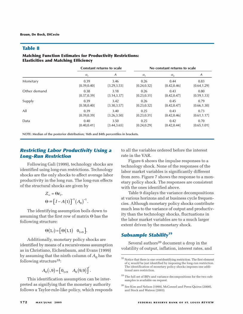
Restricting Labor Productivity Using aLong-Run Restriction

Following Galì (1999), technology shocks areidentified using long-run restrictions. Technologyshocks are the only shocks to affect average laborproductivity in the long run. The long-run effectsof the structural shocks are given by

The identifying assumption boils down toassuming that the first row of matrix Θ has thefollowing structure:

Additionally, monetary policy shocks areidentified by means of a recursiveness assumptionas in Christiano, Eichenbaum, and Evans (1999)by assuming that the ninth column of A0 has thefollowing structure18:

This identification assumption can be inter-preted as signifying that the monetary authorityfollows a Taylor-rule-like policy, which responds

Z

I A A

t∞− −

=

− ( ) ( )Θ

Θ

ε ,

.; 11

01

Θ Θ1 1 1 01 9,: , .( ) = ( ) ×

A A0 1 9 09 0 9 9:, , .( ) = ( ) ′

×

to all the variables ordered before the interestrate in the VAR.

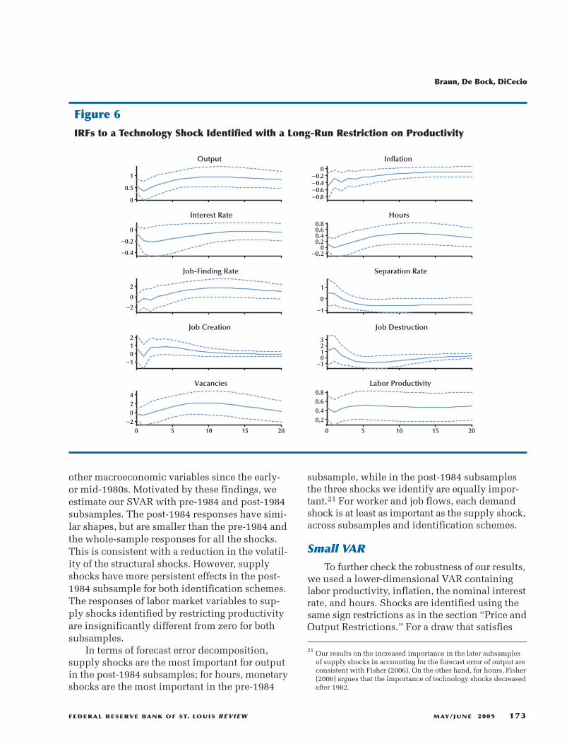
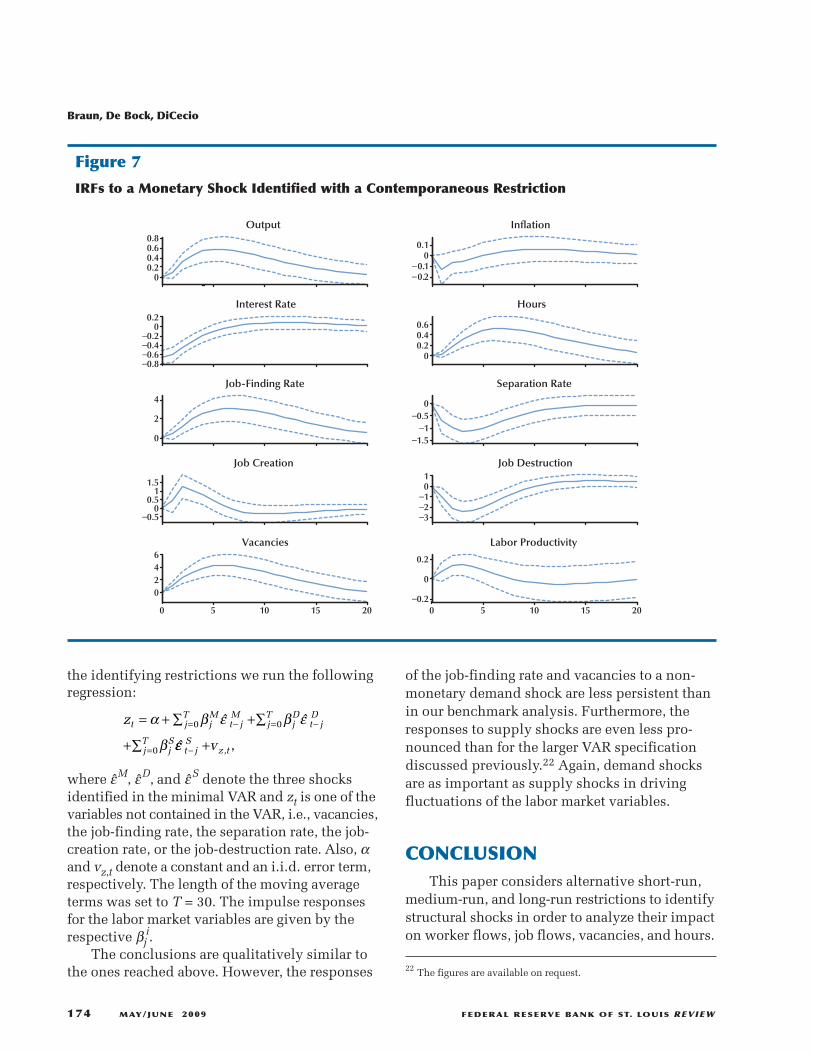
Figure 6 shows the impulse responses to atechnology shock. None of the responses of thelabor market variables is significantly differentfrom zero. Figure 7 shows the response to a mon-etary policy shock. The responses are consistentwith the ones identified above.

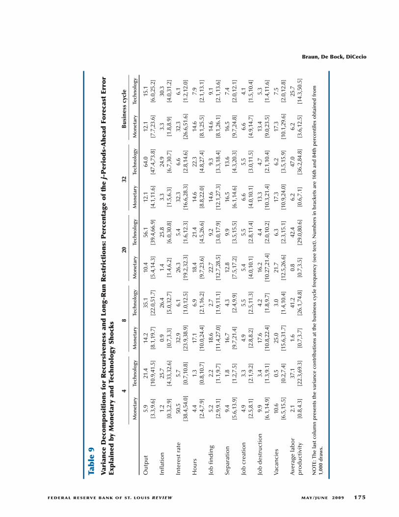
Table 9 displays the variance decompositionsat various horizons and at business cycle frequen-cies. Although monetary policy shocks contributemuch less to the variance of output and productiv-ity than the technology shocks, fluctuations inthe labor market variables are to a much largerextent driven by the monetary shock.

Subsample Stability19

Several authors20 document a drop in thevolatility of output, inflation, interest rates, and

18 Notice that there is one overidentifying restriction. The first elementof εt would be just identified by imposing the long-run restriction.The identification of monetary policy shocks imposes one addi-tional zero restriction.

19 The full set of IRFs and variance decompositions for the two sub-samples is available on request.

20 See Kim and Nelson (1999), McConnel and Perez-Quiros (2000),and Stock and Watson (2003).



Table 8Matching Function Estimates for Productivity Restrictions:Elasticities and Matching Efficiency

Constant returns to scale No constant returns to scale

αv A αv αu A

Monetary 0.39 3.46 0.26 0.44 0.83[0.39,0.40] [3.29,3.53] [0.24,0.32] [0.42,0.46] [0.64,1.29]

Other demand 0.38 3.18 0.26 0.43 0.80[0.37,0.39] [3.14,3.37] [0.23,0.31] [0.42,0.47] [0.59,1.33]

Supply 0.39 3.42 0.26 0.45 0.79[0.38,0.40] [3.30,3.57] [0.23,0.32] [0.42,0.47] [0.66,1.30]

All 0.39 3.40 0.25 0.43 0.73[0.39,0.39] [3.26,3.50] [0.23,0.31] [0.42,0.46] [0.61,1.17]

Data 0.40 3.50 0.25 0.42 0.70[0.40,0.41] [3.44,3.65] [0.24,0.29] [0.42,0.44] [0.65,1.01]

NOTE: Median of the posterior distribution; 16th and 84th percentiles in brackets.

other macroeconomic variables since the early-or mid-1980s. Motivated by these findings, weestimate our SVAR with pre-1984 and post-1984subsamples. The post-1984 responses have simi-lar shapes, but are smaller than the pre-1984 andthe whole-sample responses for all the shocks.This is consistent with a reduction in the volatil-ity of the structural shocks. However, supplyshocks have more persistent effects in the post-1984 subsample for both identification schemes.The responses of labor market variables to sup-ply shocks identified by restricting productivityare insignificantly different from zero for bothsubsamples.

In terms of forecast error decomposition,supply shocks are the most important for outputin the post-1984 subsamples; for hours, monetaryshocks are the most important in the pre-1984

subsample, while in the post-1984 subsamplesthe three shocks we identify are equally impor-tant.21 For worker and job flows, each demandshock is at least as important as the supply shock,across subsamples and identification schemes.

Small VAR

To further check the robustness of our results,we used a lower-dimensional VAR containinglabor productivity, inflation, the nominal interestrate, and hours. Shocks are identified using thesame sign restrictions as in the section “Price andOutput Restrictions.” For a draw that satisfies



21 Our results on the increased importance in the later subsamplesof supply shocks in accounting for the forecast error of output areconsistent with Fisher (2006). On the other hand, for hours, Fisher(2006) argues that the importance of technology shocks decreasedafter 1982.

0

0.5

1

Output

−0.8−0.6−0.4−0.2

0

Inflation

−0.4

−0.2

0

Interest Rate

−0.20

0.20.40.60.8

Hours

−2

0

2

Job-Finding Rate

−1

0

1

Separation Rate

−1012

Job Creation

−10123

Job Destruction

0 5 10 15 20−2

024

Vacancies

0 5 10 15 20

0.20.40.60.8

Labor Productivity

Figure 6

IRFs to a Technology Shock Identified with a Long-Run Restriction on Productivity

the identifying restrictions we run the followingregression:

where ε̂M, ε̂D, and ε̂S denote the three shocksidentified in the minimal VAR and zt is one of thevariables not contained in the VAR, i.e., vacancies,the job-finding rate, the separation rate, the job-creation rate, or the job-destruction rate. Also, αand vz,t denote a constant and an i.i.d. error term,respectively. The length of the moving averageterms was set to T = 30. The impulse responsesfor the labor market variables are given by therespective βj

i.The conclusions are qualitatively similar to

the ones reached above. However, the responses

zt jM

jT

t jM

jD

jT

t jD

jS

jT

= + ∑ +∑

+∑

= − = −

=

α β ε β ε

β0 0

0

ˆ ˆ

εε̂ t jS

z tv− + , ,

of the job-finding rate and vacancies to a non-monetary demand shock are less persistent thanin our benchmark analysis. Furthermore, theresponses to supply shocks are even less pro-nounced than for the larger VAR specificationdiscussed previously.22 Again, demand shocksare as important as supply shocks in drivingfluctuations of the labor market variables.

CONCLUSIONThis paper considers alternative short-run,

medium-run, and long-run restrictions to identifystructural shocks in order to analyze their impacton worker flows, job flows, vacancies, and hours.



00.20.40.60.8

−0.2−0.1

00.1

−0.8−0.6−0.4−0.2

00.2

00.20.40.6

0

2

4

−1.5−1

−0.50

−0.50

0.51

1.5

−3−2−101

0 5 10 15 20

0246

0 5 10 15 20−0.2

0

0.2

Output Inflation

Interest Rate Hours

Job-Finding Rate Separation Rate

Job Creation Job Destruction

Vacancies Labor Productivity

Figure 7

IRFs to a Monetary Shock Identified with a Contemporaneous Restriction

22 The figures are available on request.



Table9

Variance

DecompositionsforRecursivenessandLong-RunRestrictions:Percentage

ofthej-Periods-AheadForecastError

Explained

byMonetaryandTechnology

Shocks

48

2032

Busines

scy

cle

Monetary

Technology

Monetary

Technology

Monetary

Technology

Monetary

Technology

Monetary

Technology

Output

5.9

21.4

14.2

35.1

10.4

56.1

12.1

64.0

12.1

15.1

[3.3,9.6]

[10.9,41.5]

[8.1,19.7]

[22.0,51.7]

[5.4,14.3]

[39.4,66.9]

[4.1,11.6]

[47.4,73.8]

[7.7,23.6]

[6.0,25.2]

Inflation

1.2

25.7

0.9

26.4

1.4

25.8

3.3

24.9

3.3

30.3

[0.3,2.9]

[4.33,32.6]

[0.7,3.3]

[5.0,32.7]

[1.4,6.2]

[6.0,30.8]

[1.5,6.3]

[6.7,30.7]

[1.8,8.9]

[4.0,31.2]

Interest rate

50.5

5.7

32.9

6.1

26.3

5.4

32.3

6.6

32.3

6.1

[38.4,54.0]

[0.7,10.8]

[23.9,38.9]

[1.0,12.5]

[19.2,32.3]

[1.6,12.3]

[16.6,28.3]

[2.8,14.6]

[26.6,51.6]

[1.2,12.0]

Hours

4.4

1.3

17.1

6.9

18.4

21.4

14.6

22.3

14.6

7.9

[2.4,7.9]

[0.8,10.7]

[10.0,24.4]

[2.1,16.2]

[9.7,23.6]

[4.5,26.6]

[8.8,22.0]

[4.8,27.4]

[8.1,25.5]

[2.1,13.1]

Job finding

5.2

2.2

18.6

2.7

22.7

9.2

14.6

9.3

14.6

9.1

[2.9,9.1]

[1.1,9.7]

[11.4,27.0]

[1.9,11.1]

[12.7,28.5]

[3.0,17.9]

[12.1,27.3]

[3.3,18.4]

[8.1,26.1]

[2.1,13.6]

Separation

9.4

1.8

16.7

4.3

12.8

9.9

16.5

13.6

16.5

7.4

[5.6,13.9]

[1.2,7.5]

[9.7,21.4]

[2.4,9.9]

[7.5,17.2]

[3.5,15.5]

[6.1,14.6]

[4.3,20.3]

[9.7,24.8]

[2.0,12.1]

Job creation

4.9

3.3

4.9

5.5

5.4

5.5

6.6

5.5

6.6

4.1

[2.5,8.1]

[2.1,9.2]

[2.8,8.2]

[2.5,11.3]

[4.0,10.1]

[2.8,11.4]

[4.0,10.1]

[3.0,11.5]

[4.9,14.7]

[1.5,10.4]

Job destruction

9.9

3.4

17.6

4.2

16.2

4.4

13.3

4.7

13.4

5.3

[6.1,14.9]

[1.3,9.1]

[10.8,22.4]

[1.8,9.7]

[10.27,21.4]

[2.0,10.2]

[ 10.3,21.4]

[2.1,10.4]

[9.0,23.5]

[1.4,11.6]

Vacancies

10.6

0.5

25.0

3.0

21.7

6.3

17.3

6.2

17.3

7.5

[6.5,15.5]

[0.2,7.4]

[15.6,31.7]

[1.4,10.4]

[12.5,26.6]

[2.3,15.1]

[10.9,24.0]

[3.5,15.9]

[10.1,29.6]

[2.0,12.8]

Average labor

2.1

37.1

1.6

41.2

0.8

42.4

6.2

47.0

6.2

25.7

productivity

[0.8,4.3]

[22.3,69.3]

[0.7,3.7]

[26.1,74.8]

[0.7,3.5]

[29.0,80.6]

[0.6,7.1]

[36.2,84.8]

[3.6,12.5]

[14.3,50.5]

NOTE:The

lastcolumnpresentsthevariance

contributions

atthebusinesscyclefrequency(see

text).Num

bersinbracketsare16th

and84th

percentilesobtained

from

1,000draws.

We find that demand shocks are more importantthan supply shocks (technology shocks, morespecifically) in driving labor market fluctuations.When identified by means of short-run price andoutput restrictions, supply shocks have effectsthat are qualitatively similar to those of demandshocks: Both demand and supply shocks raiseemployment, vacancies, the job-creation rate, andthe job-finding rate while lowering unemploy-ment, separations, and job destruction. Theseeffects are more persistent for supply shocks.When identified by means of medium-run or long-run restrictions on labor productivity, supplyshocks do not have a clear effect on the labormarket variables.

REFERENCESAndolfatto, David. “Business Cycles and Labor-Market

Search.” American Economic Review, 1996, 86(1),pp. 112-32.

Basu, Susanto; Fernald, John G. and Kimball, Miles S.“Stock Prices, News and Economic Fluctuations.”NBER Working Paper No. 10548, National Bureauof Economic Research, 2004.

Basu, Susanto; Fernald, John G. and Kimball, Miles S.“Are Technology Improvements Contractionary?”American Economic Review, 2006, 96(5), pp. 1418-48.

Beaudry, Paul and Portier, Franck. “Stock Prices,News and Economic Fluctuations.” AmericanEconomic Review, 2006, 96(4), pp. 1293-307.

Blanchard, Olivier J. and Diamond, Peter. “TheCyclical Behavior of the Gross Flows of U.S.Workers.” Brookings Papers on Economic Activity,1990, 21(2), pp. 85-143.

Braun, Helge. “(Un)Employment Dynamics: The Caseof Monetary Policy Shocks.” Unpublished manu-script, University of British Columbia, 2005.

Braun, Helge; De Bock, Reinout and DiCecio, Riccardo.“Aggregate Shocks and Labor Market Fluctuations.”Working Paper No. 2006-004A, Federal ReserveBank of St. Louis, 2006.

Caballero, Ricardo J. and Hammour, Mohammad L.“The Cost of Recessions Revisited: A Reverse-Liquidationist View.” Review of Economic Studies,2005, 72(2), pp. 313–41.

Christiano, Lawrence J.; Eichenbaum, Martin andEvans, Charles L. “Monetary Policy Shocks: WhatHave We Learned and to What End?” in John B.Taylor and Michael Woodford, eds., Handbook ofMacroeconomics, Vol. 1A, Chap. 1. New York:Elsevier, 1999, pp. 65-148.

Christiano, Lawrence J.; Eichenbaum, Martin andVigfusson, Robert. “The Response of Hours to aTechnology Shock: Evidence Based on DirectMeasures of Technology.” Journal of the EuropeanEconomic Association, 2004, 2(2-3), pp. 381-95.

Christiano, Lawrence J. and Fitzgerald, Terry J. “TheBand Pass Filter.” International Economic Review,2003, 44(2), pp. 435-65.

Davis, Steven J.; Faberman, R. Jason and Haltiwanger,John C. “The Flow Approach to Labor Markets:New Data Sources, Micro-Macro Links and theRecent Downturn.” Journal of EconomicPerspectives, 2006, 20(3), pp. 3-26.

Davis, Steven J. and Haltiwanger, John C. “Gross JobCreation, Gross Job Destruction, and EmploymentReallocation.” Quarterly Journal of Economics,1992, 107(3), pp. 819-63.

Davis, Steven J. and Haltiwanger, John C. “On theDriving Forces behind Cyclical Movements inEmployment and Job Reallocation.” AmericanEconomic Review, 1999, 89(5), pp. 1234-58.

Davis, Steven J.; Haltiwanger, John C. and Schuh,Scott. Job Creation and Destruction. Boston: MITPress, 1996.

Faberman, R. Jason. “Gross Job Flows over the PastTwo Business Cycles: Not All ‘Recoveries’ AreCreated Equal.” Discussion Paper No. 372, U.S.Bureau of Labor Statistics, 2004.

Fisher, Jonas D.M. “The Dynamic Effects of Neutraland Investment-Specific Technology Shocks.”Journal of Political Economy, 2006, 114(3), pp. 413-51.



Francis, Neville; Owyang, Michael T. and Roush,Jennifer E. “A Flexible Finite-Horizon Identificationof Technology Shocks.” Working Paper No. 2005-024E, Federal Reserve Bank of St. Louis, 2008.

Francis, Neville and Ramey, Valerie A. “Is theTechnology-Driven Real Business Cycle HypothesisDead? Shocks and Aggregate Fluctuations Revisited.”Journal of Monetary Economics, 2005, 52(8), pp. 1379-99.

Fujita, Shigeru. “Vacancy Persistence.” Working PaperNo. 04-23, Federal Reserve Bank of Philadelphia,2004.

Galì, Jordi. “Technology, Employment, and theBusiness Cycle: Do Technology Shocks ExplainAggregate Fluctuations?” American EconomicReview, 1999, 89(1), pp. 249-71.

Galì, Jordi. “On the Role of Technology Shocks as aSource of Business Cycles: Some New Evidence.”Journal of the European Economic Association,2004, 2(2-3), pp. 372-80.

Hagedorn, Marcus and Manovskii, Iurii. “TheCyclical Behavior of Equilibrium Unemploymentand Vacancies Revisited.” American EconomicReview, 2008, 98(4), pp. 1692-706.

Hall, Robert E. “Job Loss, Job Finding, andUnemployment in the U.S. Economy over the PastFifty Years,” in Mark Gertler and Kenneth Rogoff,eds., NBER Macroeconomics Annual 2005, Vol. 20.Boston: MIT Press, 2006.

Jeffreys, Harold. Theory of Probability, Third Edition.London: Oxford University Press, 1961.

Kim, Chang-Jin and Nelson, Charles R. “Has TheU.S. Economy Become More Stable? A BayesianApproach Based on a Markov-Switching Model ofthe Business Cycle.” Review of Economics andStatistics, 1999, 81(4), pp. 608-16.

López-Salido, David J. and Michelacci, Claudio.“Technology Shocks and Job Flows.” Review ofEconomic Studies, 2007, 74(4), pp. 1195-227.

McConnell, Margaret M. and Perez-Quiros, Gabriel.“Output Fluctuations in the United States: What

Has Changed Since the Early 1980’s?” AmericanEconomic Review, 2000, 90(5), pp. 1464-76.

Mortensen, Dale T. and Nagypál, Éva. “More onUnemployment and Vacancy Fluctuations.” NBERWorking Paper No. 11692, National Bureau ofEconomic Research, 2005.

Mortensen, Dale T. and Pissarides, Christopher A.“Job Creation and Job Destruction in the Theory ofUnemployment.” Review of Economic Studies,1994, 61(3), pp. 397-415.

Peersman, Gert. “What Caused the Early MillenniumSlowdown? Evidence Based on VectorAutoregressions.” Journal of Applied Econometrics,2005, 20(2), pp. 185-207.

Petrongolo, Barbara and Pissarides, Christopher A.“Looking into the Black Box: A Survey of theMatching Function.” Journal of Economic Literature,2001, 39(2), pp. 390-431.

Shea, John. “What Do Technology Shocks Do?” inBen S. Bernanke and Julio J. Rotemberg, eds.,NBER Macroeconomics Annual 1998, Vol. 13.Boston: MIT Press, 1999.

Shimer, Robert. “The Consequences of Rigid Wagesin Search Models.” Journal of the EuropeanEconomic Association, 2004, 2(2-3), pp. 469-79.

Shimer, Robert. “The Cyclicality of Hires, Separations,and Job-to-Job Transitions.” Federal Reserve Bankof St. Louis Review, 2005, 87(4), pp. 493-508.

Shimer, Robert. “Reassessing the Ins and Outs ofUnemployment.” Unpublished manuscript,University of Chicago, 2007.

Silva, José I. and Toledo, Manuel. “Labor TurnoverCosts and the Cyclical Behavior of Vacancies andUnemployment.” Meeting Paper No. 775, Societyfor Economic Dynamics, 2005.

Stock, James H. and Watson, Mark W. “Has theBusiness Cycle Changed and Why?” in Mark Gertler,and Kenneth Rogoff, eds, NBER MacroeconomicsAnnual 2002, Vol. 17. Boston: MIT Press, 2003.



http://research.stlouisfed.org/publications/review/05/07/Shimer.pdf

http://research.stlouisfed.org/publications/review/05/07/Shimer.pdf

Trigari, Antonella. “Equilibrium Unemployment, JobFlows and Inflation Dynamics.” Journal of Money,Credit, and Banking, 2009, 41(1), pp. 1-33.

Uhlig, Harald. “Do Technology Shocks Lead to a Fallin Total Hours Worked?” Journal of the EuropeanEconomic Association, 2004, 2(2-3), pp. 361-71.

Uhlig, Harald. “What Are the Effects of MonetaryPolicy on Output? Results from an AgnosticIdentification Procedure.” Journal of MonetaryEconomics, 2005, 52(2), pp. 381-419.



APPENDIX

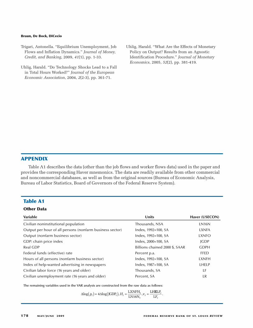
Table A1 describes the data (other than the job flows and worker flows data) used in the paper andprovides the corresponding Haver mnemonics. The data are readily available from other commercialand noncommercial databases, as well as from the original sources (Bureau of Economic Analysis,Bureau of Labor Statistics, Board of Governors of the Federal Reserve System).

Table A1Other Data

Variable Units Haver (USECON)

Civilian noninstitutional population Thousands, NSA LN16N

Output per hour of all persons (nonfarm business sector) Index, 1992=100, SA LXNFA

Output (nonfarm business sector) Index, 1992=100, SA LXNFO

GDP: chain price index Index, 2000=100, SA JGDP

Real GDP Billions chained 2000 $, SAAR GDPH

Federal funds (effective) rate Percent p.a. FFED

Hours of all persons (nonfarm business sector) Index, 1992=100, SA LXNFH

Index of help-wanted advertising in newspapers Index, 1987=100, SA LHELP

Civilian labor force (16 years and older) Thousands, SA LF

Civilian unemployment rate (16 years and older) Percent, SA LR

The remaining variables used in the VAR analysis are constructed from the raw data as follows:

∆ ∆log log JGDP ,LXNFHLN16N

,LH

p H vt t tt

tt( ) = ( ) = =4

EELPLF

.t

t

Documents

Supply Shocks, Demand Shocks, and Labor Market Fluctuations · PDF file · 2017-09-05Supply Shocks, Demand Shocks, and Labor Market Fluctuations ... Including aggregate hours