Embed Size (px)
Citation preview
UNIVERSITE DU MAINE - FACULTE DES SCIENCES ECONOMIQUES
GROUPE D’ANALYSE DES ITINERAIRES ET NIVEAUX SALARIAUX
GAINS-TEPP FR CNRS: 3126
Annee 2008
N attribue par la bibliotheque:
“Essays on Economic Fluctuations, Growth and the Labor
Market Performance: the Impact of Tax/Benefit Systems”
THESE
Pour obtenir le grade de
DOCTEUR DE L’UNIVERSITE
Discipline: Sciences Economiques
Presentee et soutenue publiquement par
Coralia Azucena QUINTERO ROJAS
le 7 mai 2008
Directeur de these:
Francois LANGOT, Professeur a l’Universite du Maine
JURY:
Jean-Olivier HAIRAULT, Rapporteur, Professeur a l’Universite Paris I
Franck PORTIER, Rapporteur, Professeur a l’Universite de Toulouse I
Henri SNEESSENS, Professeur a l’Universite Catholique de Louvain
Fabien TRIPIER, Professeur a l’Universite de Nantes
Arnaud CHERON, Professeur a l’Universite du Maine

I thank the doctoral grant from the Mexican CONACYT.
The views expressed herein are those of the authors and not necessarily those of l’Universite du
Maine.
2

Remerciements
Je tiens tout d’abord a exprimer ma reconnaissance envers mon directeur de these Francois
Langot pour avoir accepte la direction de ce travail. Je le remercie pour sa grande disponi-
bilite, ses encouragements et les nombreux conseils qu’il m’a donnes tout au long de cette these.
Mais surtout pour son amitie et l’excellente formation qu’il a su me procurer. Qu’il trouve ici
l’expression de ma profonde gratitude car mes succes sont aussi les siennes.
Ma reconnaissance va egalement a Jean-Olivier Hairault, Franck Portier, Henri Sneessens, Ar-
naud Cheron et Fabien Tripier pour avoir accepte de lire ce travail et de prendre part au jury.
Mes remerciements s’adressent egalement a Armelle Champenois et Pierre-Yves Steunou. Fi-
nalement, je voudrais remercier tous les membres du GAINS et en particulier Tarek Khaskhoussi,
qui a ete un bon compagnon de route et un grand ami. Ces annees passes en votre compagnie
ont ete un veritable plaisir.

This thesis is dedicated to my parents, Silvia and Daniel, and to my sister, Reyna, whose
encouragement have meant to me so much during the pursuit of my graduate degree and the
composition of the thesis.

Resume
Cette these s’interesse aux fluctuations economiques, au chomage et a la croissance economique.
Ces dernieres decennies, la plupart des pays europeens ont connu un ralentissement de leur
croissance economique ainsi qu’un taux de chomage eleve et persistant. Cette evolution, dite de
long terme, a ete accompagnee d’une serie de fluctuations economiques de court terme. Dans
ce contexte, cette these analyse le fonctionnement du marche du travail et son incidence sur la
performance des economies developpees. Plus precisement, nous analysons les effets de court
et de long terme de certaines distorsions jugees representatives du marche du travail des pays
europeens, tels que la fiscalite, les systemes d’indemnisation du chomage et les mecanismes de
fixation du salaire.
Le premier chapitre presente le modele canonique de cycle reel dans un contexte international. Il
s’agit de determiner un ensemble d’hypotheses visant a pallier aux defaillances du modele original
dans l’explication des fluctuations du marche du travail. L’incorporation de ces hypotheses dans
ce cadre theorique fait l’objet de la premiere partie du chapitre 2. Meme si ces amendements
du cadre canonique conduisent a une meilleure comprehension des determinants des fluctuations
economiques et de leur synchronisation entre pays, les faits concernant la dynamique des heures
et du salaire ne sont pas expliques. Ceci justifie le developpement d’une modelisation alternative
du marche du travail, presente dans la deuxieme partie de ce chapitre. Au centre de ce modele
prennent place le chomage et les liens economiques entre pays.
Ce cadre est etendu au chapitre 3 pour integrer la fiscalite, ce qui nous permet de rendre
compte de la plupart des faits de court terme. Finalement, les chapitres 4 et 5 s’interessent a
la problematique liee a la croissance economique ainsi qu’a l’evolution tendancielle du temps
du travail d’equilibre. En tenant compte des rigidites presentes sur le marche du travail, nous
fournissons une explication des phenomenes de long terme.
5
Contents
1 The canonical international real business cycle model 18
1.1 The model . . . . . . . . . . . . . . . . . . . . . . . . . . . . . . . . . . . . . . . . 20
1.1.1 The representative Firm . . . . . . . . . . . . . . . . . . . . . . . . . . . . 20
1.1.2 The representative household . . . . . . . . . . . . . . . . . . . . . . . . . 22
1.1.3 General Equilibrium . . . . . . . . . . . . . . . . . . . . . . . . . . . . . . 23
1.2 Empirical results . . . . . . . . . . . . . . . . . . . . . . . . . . . . . . . . . . . . 24
1.2.1 Solution and simulation of the model . . . . . . . . . . . . . . . . . . . . . 24
1.2.2 Qualitative Analysis . . . . . . . . . . . . . . . . . . . . . . . . . . . . . . 25
1.2.3 Quantitative Properties . . . . . . . . . . . . . . . . . . . . . . . . . . . . 33
1.2.4 Sensibility analysis . . . . . . . . . . . . . . . . . . . . . . . . . . . . . . . 35
1.3 Conclusions . . . . . . . . . . . . . . . . . . . . . . . . . . . . . . . . . . . . . . . 36
2 A survey on international real business cycles and the labor market 39
2.1 National Specialization . . . . . . . . . . . . . . . . . . . . . . . . . . . . . . . . . 42
2.1.1 Firms . . . . . . . . . . . . . . . . . . . . . . . . . . . . . . . . . . . . . . 42
2.1.2 Households . . . . . . . . . . . . . . . . . . . . . . . . . . . . . . . . . . . 44
2.1.3 General Equilibrium . . . . . . . . . . . . . . . . . . . . . . . . . . . . . . 46
2.1.4 Qualitative Analysis . . . . . . . . . . . . . . . . . . . . . . . . . . . . . . 47
2.1.5 Quantitative Properties . . . . . . . . . . . . . . . . . . . . . . . . . . . . 55
2.1.6 Restricted Asset Markets . . . . . . . . . . . . . . . . . . . . . . . . . . . 55
2.1.7 Section conclusion . . . . . . . . . . . . . . . . . . . . . . . . . . . . . . . 57
2.2 The two-sector economy . . . . . . . . . . . . . . . . . . . . . . . . . . . . . . . . 59
2.2.1 Households . . . . . . . . . . . . . . . . . . . . . . . . . . . . . . . . . . . 59
2.2.2 Firms . . . . . . . . . . . . . . . . . . . . . . . . . . . . . . . . . . . . . . 61
6
2.2.3 Equilibrium . . . . . . . . . . . . . . . . . . . . . . . . . . . . . . . . . . . 63
2.2.4 Empirical results . . . . . . . . . . . . . . . . . . . . . . . . . . . . . . . . 64
2.3 Labor market search economies . . . . . . . . . . . . . . . . . . . . . . . . . . . . 69
2.3.1 National specialization . . . . . . . . . . . . . . . . . . . . . . . . . . . . . 69
2.3.2 The single good economy . . . . . . . . . . . . . . . . . . . . . . . . . . . 73
2.3.3 Empirical results . . . . . . . . . . . . . . . . . . . . . . . . . . . . . . . . 73
2.4 Conclusion . . . . . . . . . . . . . . . . . . . . . . . . . . . . . . . . . . . . . . . 76
3 Tax/Benefit system and labor market search: reconciling the standard sepa-
rable preferences with the real wage dynamics and the international business
cycles 78
3.1 The Model . . . . . . . . . . . . . . . . . . . . . . . . . . . . . . . . . . . . . . . 82
3.1.1 Labor market flows . . . . . . . . . . . . . . . . . . . . . . . . . . . . . . . 82
3.1.2 Households . . . . . . . . . . . . . . . . . . . . . . . . . . . . . . . . . . . 82
3.1.3 Firms . . . . . . . . . . . . . . . . . . . . . . . . . . . . . . . . . . . . . . 84
3.1.4 Government . . . . . . . . . . . . . . . . . . . . . . . . . . . . . . . . . . . 85
3.1.5 Nash bargaining . . . . . . . . . . . . . . . . . . . . . . . . . . . . . . . . 85
3.1.6 Equilibrium . . . . . . . . . . . . . . . . . . . . . . . . . . . . . . . . . . . 88
3.2 Empirical results . . . . . . . . . . . . . . . . . . . . . . . . . . . . . . . . . . . . 90
3.2.1 Parameterization . . . . . . . . . . . . . . . . . . . . . . . . . . . . . . . . 90
3.2.2 Models evaluation . . . . . . . . . . . . . . . . . . . . . . . . . . . . . . . 91
3.3 Conclusion . . . . . . . . . . . . . . . . . . . . . . . . . . . . . . . . . . . . . . . 99
4 Growth, Unemployment and Tax/Benefit system in European Countries 100
4.1 Empirical Analysis . . . . . . . . . . . . . . . . . . . . . . . . . . . . . . . . . . . 102
4.1.1 The data . . . . . . . . . . . . . . . . . . . . . . . . . . . . . . . . . . . . 103
4.1.2 Growth and Unemployment at a regional level: a descriptive analysis . . . 103
4.1.3 Recovering the missing link: an econometric analysis . . . . . . . . . . . . 107
4.2 The model . . . . . . . . . . . . . . . . . . . . . . . . . . . . . . . . . . . . . . . . 117
4.2.1 Preferences . . . . . . . . . . . . . . . . . . . . . . . . . . . . . . . . . . . 117
4.2.2 Goods sector . . . . . . . . . . . . . . . . . . . . . . . . . . . . . . . . . . 117
4.2.3 R&D sector . . . . . . . . . . . . . . . . . . . . . . . . . . . . . . . . . . . 118
4.2.4 Government . . . . . . . . . . . . . . . . . . . . . . . . . . . . . . . . . . . 119
7
4.2.5 Wage bargaining and labor demand . . . . . . . . . . . . . . . . . . . . . 119
4.2.6 Equilibrium . . . . . . . . . . . . . . . . . . . . . . . . . . . . . . . . . . . 119
4.3 The impact of labor market institutions on growth and unemployment . . . . . . 121
4.3.1 Labor market policies . . . . . . . . . . . . . . . . . . . . . . . . . . . . . 121
4.3.2 The wage bargaining processes . . . . . . . . . . . . . . . . . . . . . . . . 121
4.4 Conclusion . . . . . . . . . . . . . . . . . . . . . . . . . . . . . . . . . . . . . . . 123
5 Explaining the evolution of hours worked and employment across OECD
countries: an equilibrium search approach 124
5.1 Stylized Facts . . . . . . . . . . . . . . . . . . . . . . . . . . . . . . . . . . . . . . 127
5.2 Walrasian growth model . . . . . . . . . . . . . . . . . . . . . . . . . . . . . . . . 130
5.2.1 When only the intensive margin is endogenous . . . . . . . . . . . . . . . 130
5.2.2 When only the extensive margin is endogenous . . . . . . . . . . . . . . . 137
5.3 Search model with intensive and extensive margins . . . . . . . . . . . . . . . . . 142
5.3.1 The equilibrium matching model . . . . . . . . . . . . . . . . . . . . . . . 142
5.3.2 Calibration and data . . . . . . . . . . . . . . . . . . . . . . . . . . . . . . 147
5.3.3 Empirical results . . . . . . . . . . . . . . . . . . . . . . . . . . . . . . . . 150
5.4 Conclusion . . . . . . . . . . . . . . . . . . . . . . . . . . . . . . . . . . . . . . . 157
A Appendix to chapter 1 168
A.1 Sensitivity analysis of the instantaneous elasticities . . . . . . . . . . . . . . . . . 168
B Appendix to chapter 2 170
B.1 National specialization economy . . . . . . . . . . . . . . . . . . . . . . . . . . . . 170
B.2 Two-sectors economy . . . . . . . . . . . . . . . . . . . . . . . . . . . . . . . . . . 172
C Appendix to chapter 4 174
C.1 Proofs . . . . . . . . . . . . . . . . . . . . . . . . . . . . . . . . . . . . . . . . . . 174
D Reaching the Optimal Growth:
Which is the role of the Labor Market Institutions? 175
D.1 The model . . . . . . . . . . . . . . . . . . . . . . . . . . . . . . . . . . . . . . . . 176
D.1.1 Preferences . . . . . . . . . . . . . . . . . . . . . . . . . . . . . . . . . . . 176
D.1.2 Goods sector . . . . . . . . . . . . . . . . . . . . . . . . . . . . . . . . . . 176
8
D.1.3 R&D sector . . . . . . . . . . . . . . . . . . . . . . . . . . . . . . . . . . . 177
D.1.4 Government . . . . . . . . . . . . . . . . . . . . . . . . . . . . . . . . . . . 177
D.1.5 Wage bargaining and labor demand . . . . . . . . . . . . . . . . . . . . . 177
D.1.6 Equilibrium . . . . . . . . . . . . . . . . . . . . . . . . . . . . . . . . . . . 178
D.1.7 The optimal economic growth . . . . . . . . . . . . . . . . . . . . . . . . . 178
D.1.8 Equilibrium growth v.s. optimal growth . . . . . . . . . . . . . . . . . . . 179
E Appendix to chapter 5 181
E.1 Data . . . . . . . . . . . . . . . . . . . . . . . . . . . . . . . . . . . . . . . . . . . 181
E.2 The Hansen-Rorgerson economy by country . . . . . . . . . . . . . . . . . . . . . 182
9
Introduction
Last decades, continental European countries have experienced high and persistent unemploy-
ment, and a slowdown of economic growth. In parallel, aggregate hours of market work exhibit
dramatic differences across industrialized countries, whereas the aggregate hours worked have
decrease relative to the United States. Moreover, this evolution has been accompanied by recur-
rent fluctuations in the economies’ incomes, products, and factor inputs, especially labor, that
are due to nonmonetary sources. Against this background, this dissertation tries to gain insight
on the identification of the key factors that shape the short-run and the long-run evolution of
the labor market of the industrialized economies.
To this goal, two parts are distinguished. Part I focuses on the short run issues and is divided
in three chapters. Chapter 1 sets up the basis of our study on international fluctuations and the
labor market. We expose there the properties of an international general equilibrium model in
which all markets are assumed to be walrasian and fluctuations are solely driven by stochastic
technological impulsions. The detailed analysis of this framework, that we regard as the canon-
ical international real business cycle (thereafter, IRBC) model, let us identify its limits and is
essential to appreciate the empirical relevance of each new hypothesis incorporated along the
subsequent chapters.
This chapter is as well a methodological one. We present the standard solution method, and
we conduct sensitivity analysis to get a better understanding of the basic mechanisms at work.
This let us assess the role played by two key parameters: the first one related to the adjustment
costs of capital, and the second one to the elasticity of labor. As well, at each time we compare
the implications from two specifications of the agents’ preferences. The first one assumes a
standard separability between consumption and leisure, whereas the second one assumes a non-
separability between them. The canonical IRBC model developed in chapter 1 appears to be
insufficient to account for most of the international features of business cycles. Moreover, it has
10

the same limitations as its closed-economy counterpart regarding the dynamics of the real wage,
the labor productivity and the total hours.
According to these results, chapter 2 exposes a survey of several standard amendments intended
to improve the predictions of the model. This survey is restricted to issues that are directly
related to the real economy. The first extension aims to deep the link between the home and
the foreign countries. To this end we introduce an additional consumption/investment good by
considering national specialization (Backus, Kehoe, and Kydland 1994). This richer structure
adds a new mechanism by which the expansion of output experienced in the country receiving
the shock, may induce an expansion of output in the other country. This potentially allows for
positive cross-correlations for labor inputs and investments. Even if this ameliorates the theo-
retical predictions relative to the international facts, the model is far to be sufficient. Following
Galı (1994), we also distinguish the composite good for consumption from the composite good
for investment. However, this does not change the predictions of the model since we allow for
perfect competitive markets.
The second extension aims to reduce the international correlation of consumptions. This is done
by restricting international trade to non-contingent bonds (Baxter 1995). This limitation in
the agent’s ability to risk pooling country-specific shocks produces more realistic international
correlations of outputs and consumptions. However, the correlation of outputs still larger than
the one of consumptions.
The last extension in the pure walrasian framework that we consider is the introduction of a
realistic potential for intra- and international capital flows by the disaggregation of the economy
into internationally traded and non-traded sectors (Stockman and Tesar 1995). This is justified
by the empirical evidence that roughly a half of the typical G-10 country’s output consists of
non-traded goods and services. It must be enhanced that, conversely to traditional IRBC models
with only technological shocks, as the Stockman and Tesar (1995)’s model, our model predicts
positive international comovements of production inputs, which is more in accordance with the
empirical correlations, but they are overstated particularly when shocks are highly persistent.
Nevertheless, because at this point we have not yet modified the walrasian nature of the labor
market, all models still fail in reproducing the fluctuations of the employment, the hours worked
and the real wage. Hence, the next step is to modify the walrasian labor market by introducing
search and matching in the labor market. This is the core of the second part of this survey,
in which we take as starting point the Hairault (2002)’s two-country, two-good search economy
11

to going ahead in the study of some stylized facts of the US labor market. Next, we make
a reduction to the single-good case to assess the role of the key hypotheses in the Hairault’s
economy. Namely, (i) the non-separability between consumption and leisure in the agents’
preferences, (ii) the existence of two goods in the world and so of one relative price, and (iii)
search and bargaining in the labor market. In this single-good search framework we also evaluate
the predictions from the model with restricted international trade to non-contingent bonds.
However, we do not extend the search model to include two sectors because the results from the
walrasian economy are discouraging.
There we show that in the single-good economy, the combination of search and matching in the
labor market with the non-separability is enough to predict positive comovements of labor inputs
and investments as well as a large dissociation of consumptions. Moreover, the procyclicality
of real wage rate is reduced, and the correlation of total hours with both output and labor
productivity is lower. Then, the three puzzles are partially solved. However, consumptions
correlation still larger than outputs correlation, even if the incompleteness of financial markets
produces more realistic international correlations of outputs and consumptions. Then, we show
that the gain from including two goods in that framework is that the model is able now to
replicate a correlation of outputs bigger than the one of consumptions (Hairault 2002). However,
the price dynamics provoked by a positive productivity shock decrease the agent’s purchasing
power, leading to a stronger vindication of salary and so to a slightly more procyclical real wage.
To sum up the first two chapters, we can say that, relative to the data, in the walrasian extensions
the variability of consumption, hours of work, and output is too low, and the variability of
investment is too high. But maybe the main failure is the predicted correlation of real wages
with both hours worked and output. In such a models, variations in technology shifts the labor
demand curve but not the labor supply curve, thus inducing a strong positive correlation between
wages and hours. The introduction of search and matching in the labor market (Andolfatto 1996)
outperforms the model predictions. But the volatility of total hours still underestimated, and
the real wage still procyclical.
This line of reasoning naturally suggests that to improve the predictions from the real business
cycle models one must include something that shifts labor supply. If both labor demand and
labor supply shift, then the strong positive correlation between hours and wages can probably
be reduced. So, in chapter 3 we study the short run effects of fiscal policy in a search framework.
In the Keynesian tradition, fiscal policy, and therefore taxation, is one of the main instruments
12
to stabilize the economy. However, in the 1990s, several pioneering works considered taxation
as a source of business cycle fluctuations (Christiano and Eichenbaum (1992), Braun (1994),
McGrattan (1994), ?)). This feeds the criticisms about the possibility to use taxes as stabilization
tool. These pioneering articles have shown that stochastic fiscal policy improves the performance
of real business cycle models. Intuitively, shocks to income and payroll taxes can be interpreted
as shocks to labor supply, as opposed to technology shocks which may be interpreted as shocks
to labor demand. Thus, tax rates provide another mechanism for explaining the observed
correlation between hours and wages.
In quantitative terms, these former works yield to predictions for the correlation between hours
and real wages, as measured by average productivity, closer to the empirical correlation. Like-
wise, the predicted variability of hours worked and consumption are much closer to their empir-
ical values when fiscal policy is included (even if in general the relative volatility of aggregate
hours is overstated). Nevertheless, these former papers show two drawbacks. The first one is
that all of them consider a closed economy, so that the possible variability in the macro aggre-
gates passing through the international trade is not accounted for. The second one is that the
theoretical real wage is measured by the average productivity. This obviously prevents from
analyzing other features of the US labor market, such as the lower volatility of the real wage
with respect to the volatility of the labor productivity.
By contrast, in chapter 3 we show that fluctuations in distortive taxes can account for some
of the puzzling features of the U.S. business cycle. Namely, the observed real wage rigidity,
the international comovement of investment and labor inputs, and the so-called consumption
correlation puzzle (according to which cross-country correlations of output are higher than the
one of consumption). This is done in a two-country search and matching model with fairly
standard preferences, extended to include a tax/benefit system. In this simple framework, the
tax side is represented by taxation on labor income, employment (payroll tax) and consumption,
whereas the benefit side is resumed by the unemployment benefits and the worker’s bargaining
power.
Then, the main departures from the former literature on taxation as a source of business cycle
fluctuations are twofold. First, we consider a two-country general equilibrium model, so that
we are able to discuss the effects on the observed international fluctuations. Second, we assume
search and matching in the labor market. Our model is close to the Hairault (2002)’s one, who
develops a two-country, two-good search model, able to explain the puzzling facts of international
13
fluctuations once a non-separability in the agents’ preferences is considered. Our model is also
close to the Cheron and Langot (2004)’s model, who explain the real wage rigidity in a closed-
economy search model by means of a particular set of non-separable preferences.
Either in the Hairault (2002)’s paper or in the Cheron and Langot (2004)’s paper, the non-
separability of preferences plays a main role. However, this hypothesis is unable to simultane-
ously account for the real wage rigidity and for the observed international fluctuations. Con-
versely, we show that all those facts can be accounted in a single framework with fairly standard
separable preferences. These new results concerning business cycle theory provide support to
the matching models.
Part II is concerned with the long term issues and is composed of two chapters. In chapter 4
we investigate the issue of the long run link between growth and unemployment at two levels.
First, we conduct an empirical analysis to explore the heterogeneity of growth and unemploy-
ment experiences across 183 European regions from 1980 to 2003 and we evaluate how much
of this heterogeneity is accounted by the national labor market institutions. One originality of
this approach is to take into account the large heterogeneity between regions among a country.
Second, we construct a theoretical economy to assess the explicative role of labor-market vari-
ables on the bad performance of European countries. The main hypotheses of our model are
the following: (i) Innovations are the engine of growth. This implies a “creative destruction”
process generating jobs reallocation. (ii) Agents have the choice of being employed or being
trying their hand at R&D; and (iii) Unemployment is caused both by the wage-setting behavior
of unions, and by the labor costs associated to the tax/benefit system.1
The advises from the empirical exercise are that: (i) The tax wedge and the unemployment
benefits are positively correlated with the regional unemployment rates. Conversely, the em-
ployment protection and the level of coordination in the wage bargaining process are negatively
correlated with the regional unemployment rates. (ii) The tax wedge and the unemployment
benefits are negatively correlated with the regional growth rates of the Gross Domestic Product
(GDP) per capita. Conversely, more coordination in the wage bargaining process diminishes
the regional growth rates of GDP per capita. This last result points to the existence of an
arbitration between unemployment and growth, if we focuss on the impact of coordination in
the wage bargaining process. These results are in accordance with the country-level results of
Daveri and Tabellini (2000).1The two first hypotheses are the same as those of Aghion and Howitt (1994).
14

On the other side, the implications of the theoretical model are the following: (i) The bargain-
ing power of unions, the unemployment compensation, the taxes on labor and the employment
protection have a positive effect on unemployment and a negative effect on the economic growth.
(ii) A more coordinated bargaining process increases employment, at the price of a lower eco-
nomic growth. The first result clearly contrast with the results of Lingens (2003) and Mortensen
(2005). Lingens (2003) treats the impact of unions in a model with two kind of skills, and shows
that the bargain over the low-skilled labor wage causes unemployment but the growth effect is
ambiguous. Similarly, in a matching model of schumpeterian growth, Mortensen (2005) finds a
negative effect of labor market policy on unemployment, but an ambiguous effect on growth.
Finally, chapter 5 studies the dynamics of aggregate hours of market work, which exhibit dra-
matic differences across industrialized countries, either at points of time across countries, or
within a country over time. In the current literature, there are two candidate approaches allow-
ing to explain these differences. A first set of contributions focuses on the decline of the average
hours worked per employee (the intensive margin) in European countries since 1960. Prescott
(2004) studies the role of taxes in accounting for differences in labor supply across time and
across countries. He finds that the effective marginal tax rate on labor income explains most of
the differences at points of time and the large change in relative (to US) labor supply over time.
On this line of research, Rogerson (2006) shows that the aggregate hours worked in Continental
European countries such as Belgium, France, Germany and Italy are roughly one third less than
in the US. This fact results from a diverging process in the hours worked per employee in each
zone: between 1960 and 1980, whereas in Europe we observe a large decrease, in the US this
decline is very small; and after 1980, we observe in the two zones a stable number of hours
worked per employee. This evolution of the hours worked per employee is strongly correlated
to the dynamics of the taxes. Hence, as it is suggested by Prescott (2004), Rogerson (2006) or
Ohanian, Raffo, and Rogerson (2006), a theory providing a link between the hours worked per
employee and taxes seems to be sufficient to explain why Europeans work less than Americans.
However, since 1980 a notable feature of the data is that differences across countries in aggregate
hours are due to quantitatively important differences along the extensive margin. Hence, a
second set of contributions (see e.g. Jackman, Layard, and Nickell (1991), Mortensen and
Pissarides (1999a), Blanchard and Wolfers (2000) or Ljungqvist and Sargent (2007b)) considers
that the large decrease of the employment rate observed after 1980 in the European countries, is
an important factor of the dynamics of total hours. These works show that different labor market
15
institutions lead to different labor market outcomes after a common shock. In these previous
papers, there is fairly robust evidence that (i) the level and duration of unemployment benefits
and (ii) the union’s bargaining power have a significant positive impact on unemployment.
To sum up, the main factors explaining the decline in the hours worked per employee differ from
those explaining the decline in the employment rate: the taxes for the former, and the labor
market institutions, such as the unions’ power or the unemployment benefits, for the second.
Clearly, all together contribute to the dynamics of the two margins of the total hours.
From a theoretical point of view, the aim of this chapter is to provide a theory allowing to
account for the impact, of both taxes and labor market institutions, on the two margins of the
aggregate hours worked. To this end, we follow the empirical methodology presented in Ohanian,
Raffo, and Rogerson (2006): the quantitative evaluation of the several models and the impact
of distortions is based on the computation of series for the gap between the marginal cost and
the marginal return of labor that is produced using actual data and model restrictions2. Fur-
thermore, we extend the theoretical investigation: beyond the usual neo-classical growth model
which allows to predict the hours worked per employee, we explore the ability of the Hansen
(1985)-Rogerson (1988) model to reproduce the dynamics of the employment rate. Finally, we
develop a general equilibrium matching model, close to the one proposed by Andolfatto (1996),
Feve and Langot (1996) and Cheron and Langot (2004), allowing to explain the dynamics of
both the hours worked per employee and the employment rate. This last model is rich enough
to allow the evaluation of the relative contribution of the tax/benefit systems and unions in the
explanation of the observed allocation of time.
The main findings of last chapter are the following. First, the long-run decline in the hours
worked per employee is mainly due to the increase of the taxes, as it is suggested by Prescott
(2004), Rogerson (2006) and Ohanian, Raffo, and Rogerson (2006). Second, the employment
rate is affected by institutional aspects of the labor market, such as the bargaining power and the
unemployment benefits, rather than by taxes, conversely to the individual work effort. Finally,
this behavior of the two margins of the aggregate hours is well accounted by our search model,
when it includes the observed heterogeneity of the tax/benefit systems and the labor market
indicators of the wage-setting process across countries. These findings give some support to the
two explanations of the European decline in total hours: the important role of taxes through
the intensive margin and the large contribution of the labor market institutions through the2The closer these gaps are to zero, the better the model accounts for the observed labor behavior.
16

extensive margin. Because these findings come from an unified framework, they also give a
strong support to the matching models.
17

Chapter 1
The canonical international real
business cycle model
18
Introduction
This chapter is attempted to set up the basis of our study on international fluctuations and
the labor market. To this end, we expose the properties of an international general equilibrium
model in which all markets are assumed to be walrasian and fluctuations are solely driven by
stochastic technological impulsions. The detailed analysis of this framework, that we regard as
the canonical international real business cycle (thereafter, IRBC) model, let us identify its limits
and is essential to appreciate the empirical relevance of each new hypothesis incorporated along
the subsequent chapters.
This chapter is as well a methodological one. We present the standard solution method, and
we conduct several sensitivity analysis to get a better understanding of the basic mechanisms
at work. This let us assess the role played by two key parameters: the first one related to the
adjustment costs of capital, and the second one to the elasticity of labor. Moreover, at each
time we compare the results obtained from two specifications of the agents’ preferences. The
first one assumes a standard separability between consumption and leisure, whereas the second
one assumes a non-separability between them.
Since there is a single good, international trade takes place only to smooth consumption and
to ensure that capital is allocated in the most productive country. We show that, regarding
the international context, the canonical IRBC model is able to reproduce two characteristics of
developed economies:
• The net exports and the trade balance (measured as the ratio of net exports to output)
are counter-cyclical.
• Saving and investment rates are highly correlated.
However, the model is unable to replicate two major facts of developed economies:
• Interdependency (Baxter 1995): the cross correlations for production, consumption, in-
vestment and labor input are positive across countries.
• (Backus, Kehoe, and Kydland 1995) The cross-country correlation of outputs is larger
than the one of consumptions.
Moreover, regarding within country business-cycle facts, the striking limits of the model concern,
as its close-economy counterpart, the labor market fluctuations:
19
• The dynamics of the hours worked is not reproduced by the model.
• The real wage is highly pro-cyclical in the model, conversely to the data.
In addition, due to the single-good nature of the canonical model, the facts involving interna-
tional prices, such as the terms of trade or the real exchange rate, are obviously left unexplained.
1.1 The model
The world economy consists of two countries (country 1 or home country and country 2 or
foreign country), each represented by a large number of identical consumers and a production
technology. The countries produce the same final good, which is used for consumption and
investment purposes, and their preferences and technologies have the same structure and pa-
rameter values. Although, the technologies differ in two important aspects: in each country, the
labor input consists only of domestic labor, and production is subjected to idiosyncratic shocks
to productivity.1 Markets are complete: agents may trade any contingent claims they wish.
Since there is a single good, international trade takes place only to smooth consumption and to
ensure that capital is allocated in the most productive country.
1.1.1 The representative Firm
The representative firm in country i = 1, 2 produce the single good with a constant returns to
scale technology using capital Ki,t and labor Hi,t as inputs2,
Yi,t = ai,tKαi,tH
1−αi,t (1.1)
The variables ai,t represent the stochastic component of the productivity variable and are as-
sumed to follow the stationary vector-autoregressive process given bylog a1,t
log a2,t
=
ρa,1 ρa
12
ρa12 ρa2
log a1,t−1
log a2,t−1
+
1− ρa1 −ρa
12
−ρa12 1− ρa2
log a1
log a2
+
1 ψ
ψ 1
ε1,t
ε2,t
(1.2)
were the innovations ε = [ε1, ε2]′ are serially independent: E(ε1) = E(ε2) = 0, E(ε21) = σ2
ε1
E(ε22) = σ2
ε2, and E(ε1ε2) = 0 for all t. Under this specification, innovations to productivity
that originate in one country (ε1 or ε2) are transmitted to the other country if the ”spill-over”1This model is very close to the Baxter and Crucini (1993)’s model.2To simplify, we abstract from the deterministic growth rate.
20
parameters, ρa12, ρa
21 and ψ are different from zero. Because of the symmetry assumption we
impose ρa1 = ρa2 and ρa12 = ρa
21.
New capital goods are internationally mobile and all investment is subject to adjustment costs.
Capital adjustment costs have been incorporated to slowdown the response of investment to
location-specific shocks, due to the strong incentive of capital owners to locate new investment
in the most productive place. Since we are interested on the dynamics of the model near to
the steady state, we do not need to specify a particular functional form for adjustment costs.
However, to simplify the computations we suppose the following quadratic expression for the
adjustment costs:
Ci,t =φ
2(Ki,t+1 −Ki,t)2 (1.3)
Capital accumulates over time according to
Ki,t+1 = (1− δ)Ki,t + Ii,t (1.4)
Then, the Firms’ program is dynamic and consists of maximizing the expected discounted sum
of profit flows, contingent to the state At+1,
maxHi,t,Ii,t
E0
∞∑
t=0
∫vt(Yi,t − Ci,t − Ii,t − wi,tHi,t)dAt+1 (1.5)
subject to the production constraint (1.1) and to the capital constraint (1.4). vt = v(At+1) is
the factor actualization of the Firm and wi the wage rate in country i. This program can be
written in recursive form and the solution satisfies the Bellman’s equation,
W(Ki,t) = maxHi,t,Ki,t+1
Yi,t − Ci,t −Ki,t+1 + (1− δ)Ki,t − wi,tHi,t +
∫vtW(Ki,t+1)dAt+1
(1.6)
The optimal demands for labor and capital are
wi,t = (1− α)Yi,t
Hi,t(1.7)
qi,t =∫
vt∂W(Ki,t+1)
∂Ki,t+1dAt+1 (1.8)
with qi,t defined by
qi,t ≡ 1 + φ(Ii,t − δKi,t) (1.9)
Using the envelop condition for the state variable, ∂W(Ki,t)∂Ki,t
= αYi,t
Ki,t+ qi,t − δ, equation (1.8)
becomes
qi,t =∫
vt
(α
Yi,t+1
Ki,t+1+ qi,t+1 − δ
)dAt+1 (1.10)
21

Finally, we impose the following transversality condition,
limj→∞
Et[qi,t+j+1Kt+j+1] = 0 (1.11)
1.1.2 The representative household
As in the canonical model for a closed economy, the dynamics of the model rely on savings
and on the labor supply behavior following a technological shock. The labor supply behavior
depends in turn on the household’s preferences:
E0
∞∑
t=0
βtU(Ci,t, 1−Hi,t) (1.12)
where U(Ci,t, Li,t) ≡ Ui,t denotes the instantaneous utility function. Ci,t stands for the house-
hold’s consumption, whereas Li,t = 1 −Hi,t stands for the amount of leisure enjoyed at period
t.3
Financial markets are complete. At each date t households have access to contingent claims,
at price vt = v(At+1), providing one unit of the single good if the state A occurs at t + 1. We
denote by f(A) ≡ f(At+1, At) the density function describing the evolution from the state At
to the state At+1.
So, given the wage rate proposed by the Firm, wi,t, the representative household’s aims at
choosing a contingency plan Ci,t,Hi,t that maximizes (1.12) subject to the budget constraint
Ci,t +∫
vtBi(At+1)dAt+1 ≤ BiAt + wi,tHi,t (λi,t) (1.13)
were Bi,t ≡ Bi(At) denotes the household’s portfolio of contingent bonds, and λi,t the shadow
price associated to the budget constraint.
The households’ program can be written in a recursive way and its optimal solution verifies the
Bellman equation
V(Bi,t) = maxCi,t,Hi,t,Bi,t+1
Ui,t + β
∫V(Bi,t+1)f(A)dAt+1
(1.14)
subject to the budget constraint (1.13). The optimality conditions are,
∂Ui,t
∂Ci,t= λi,t (1.15)
∂Ui,t
∂Hi,t= λi,twi,t (1.16)
3The function U is assumed to be strictly increasing, concave, twice continuously differentiable and to satisfy
the Inada conditions. Moreover, C and L are assumed to be normal goods in order to guarantee the existence of
a saddle point at the general equilibrium.
22

Then, the household’s labor supply is such that the marginal utility of leisure is equal to the
wage, expressed in utility terms (since λi,t is equal to the marginal utility of consumption),
i.e. , equal to the marginal value of one hour worked. The optimal choice of contingent bonds
determines the interest rate on the international financial market:
β∂V(Bi,t+1)
∂Bi,t+1= vtλi,t (1.17)
Using the envelop condition for Bi,t:∂V(Bi,t)
∂Bi,t= λi,t, equation (1.17) can be written as
vt = βλi,t+1
λi,tf(At+1) (1.18)
Lastly, the transversality condition ensures that the marginal value of bonds holdings, in utility
units, is null at the end of the household’s life:
limj→∞
Et[βt+jλi,t+jBi,t+j+1] = 0 (1.19)
1.1.3 General Equilibrium
The equilibrium of this economy consists of a set of households’ optimal decision rules Ci(·),Hsi (·), Bi(·),
the firms’ optimal demands of capital and labor Kdi (·),Hd
i (·) and a vector of prices equilibrat-
ing the goods market, the labor market and the financial market.
Goods Market: The world constraint for the single good of this economy satisfies:
Y1,t + Y2,t = C1,t + C2,t + I1,t + I2,t + C1,t + C2,t (1.20)
Labor Market: Together, equations (1.15) and (3.24) determine the instantaneous rate of
substitution between leisure and consumption as a function of the real wage,
∂Ui,t
∂Hi,t
∂Ui,t
∂Ci,t
= wi,t (1.21)
Thus, the wage rate corresponds to the marginal gain of leisure expressed in consumption units.
Notice that, as consumption and leisure are normal goods, both vary in the same way for a given
wage, which is in stark contradiction with data.
Moreover, the equilibrium in the labor market implies that labor is remunerated at its marginal
productivity,
(1− α)Yi,t
Hi,t= wi,t (1.22)
23

Financial Market: Equation (1.17) implies that λ1,t+1
λ1,t= λ2,t+1
λ2,t= Λ ⇔ λ2,t
λ1,t= λ2,t+1
λ1,t+1= Λ′ ⇔
λ2,t = Λ′λ1,t. If we suppose that the initial wealth is the same for each individual (i.e. Λ′ = 1)
then λ2,t = λ1,t ≡ λt. Then, we can rewrite the evolution of the firm’s implicit price (equation
(1.9)) as
qi,t = β
∫λt+1
λt
(α
Yi,t+1
Ki,t+1+ qi,t+1 − δ
)f(At+1)dAt+1 ≡ βEt
[λt+1
λt
(α
Yi,t+1
Ki,t+1+ qi,t+1 − δ
)](1.23)
1.2 Empirical results
First of all, we have to specify the utility function. Throughout this thesis, we will consider two
quite standard functions: a separable utility between consumption and leisure:
Ui,t = log(Ci,t) + σ(1−Hi,t)1−η
1− η, η > 0, (1.24)
and a non-separable utility:
Ui,t = log(
Ci,t + σ(1−Hi,t)1−η
1− η
), η > 0 (1.25)
In the first case, the household’s optimal choices take the form
1Ci,t
= λt (1.26)
Ci,tσ(1−Hi,t)−η = wi,t (1.27)
whereas in the second case,
1
Ci,t + σ(1−Hi,t)1−η
1−η
= λt (1.28)
σ(1−Hi,t)−η = wi,t (1.29)
The theoretical implications of this utility specifications will be analyzed below. However, at
this stage we remark that, at equilibrium, the separability of preferences implies C1,t = C2,t ∀t(see equations (1.26)). Conversely, the equalization of consumption across countries does not
longer hold with non-separable preferences (see equations (1.28)).
1.2.1 Solution and simulation of the model
The resolution strategy is to approximate the optimality and equilibrium conditions linearly
around the steady state and to solve the resulting dynamic system. The approximate solution
24
can then be written in the state-space form as
K1,t+1
K2,t+1
a1,t+1
a2,t+1
=
µ1 µ2 π1Ka π2
Ka
µ2 µ1 π2Ka π1
Ka
0 0 ρa ρ12
0 0 ρ12 ρa
︸ ︷︷ ︸MSS
K1,t
K2,t
a1,t
a2,t
+
0 0
0 0
1 ψ
ψ 1
︸ ︷︷ ︸MSE
ε1,t+1
ε2,t+1
(1.30)
and
C1,t
C2,t
I1,t
I2,t
H1,t
H2,t
Y1,t
Y2,t
λt
w1,t
w2,t
=
ΠC1K1 ΠC1K2 ΠC1a1 ΠC1a2
ΠC2K1 ΠC2K2 ΠC2a1 ΠC2a2
ΠI1K1 ΠI1K2 ΠI1a1 ΠI1a2
ΠI2K1 ΠI2K2 ΠI2a1 ΠI2a2
ΠH1K1 ΠH1K2 ΠH1a1 ΠH1a2
ΠH2K1 ΠH2K2 ΠH2a1 ΠH2a2
ΠY1K1 ΠY1K2 ΠY1a1 ΠY1a2
ΠY2K1 ΠY2K2 ΠY2a1 ΠY2a2
ΠλK1 ΠλK2 Πλa1 Πλa2
Πw1K1 Πw1K2 Πw1a1 Πw1a2
Πw2K1 Πw2K2 Πw2a1 Πw2a2
︸ ︷︷ ︸Π
K1,t
K2,t
a1,t
a2,t
(1.31)
The matrices MSS and Π are composed of instantaneous elasticities, which are non-linear com-
binations of the structural parameters of the model. Then, for a given set of parameter values,
we will be able to analyze the responses of the variables to an idiosyncratic technological shock,
as well as to compute the cyclical properties of the model (i.e. , the second order moments).
The Impulse Response Functions (IRF) are computed from the two last expressions.
1.2.2 Qualitative Analysis
Steady State and calibration of the structural parameters
H is fixed to 1/3 and we calculate η such that the average individual labor supply elasticity is
equal to 1η
1−HH = 2
3 ⇒ η = 3, a value consistent with the bulk of empirical estimates. The Tobin’s
q is set equal to unity (Baxter and Crucini 1993). φ, the capital adjustment cost parameter, is
calibrated in order to replicate the volatility of investment in the economy with non-separable
preferences and international transmission of the shock (IRBC1b-NSP). We keep it constant
across the other simulations in order to isolate the intrinsic properties of the different models.
We normalize a = 1, then we can compute the steady-state values for the remaining variables
25

as
K =(
1/β − 1 + δ
αH1−α
) 1α−1
Y = KαH1−α
I = δK
C = Y − I
w = (1− α)Y
K
If preferences are separable between consumption and leisure, then
λ = 1/C
σ =w
C(1−H)−η
Else,
σ =w
(1−H)−η
λ =1
C + σ (1−H)1−η
1−η
Table 1.1: Benchmark calibration.
α β H η φ δ ρa ρa12 ψ σεa σ σ
0.36 0.99 1/3 3 0.056 0.025 0.906 0 0 0.00852 0.7508 0.6804
Responses to a technological shock
Matter of clarity, we take as benchmark the simplest case in which a positive 1% productivity
shock arrives to country 1, but it is no transmitted to country 2: ψ = ρa12 = 0. The values for
ρa and σεa are taken from Backus, Kehoe, and Kydland (1994), while the remaining parameters
come from Hairault (2002) (See Table 1). This corresponds to the framework analyzed by
Devereux, Gregory, and Smith (1992). The IRF are shown in figure 1.2, for separable preferences
(IRBC1a-SP), and in figure 1.4, for non-separable preferences (IRBC1a-NSP). The responses of
the country 1 variables at impact are as follows:
26
The instantaneous response of output (≈ 1.28%) is due to the direct effect of the productivity
shock and to the increase in labor, as can be seen from the log-linear expression of output:
Y1,t = a1,t + (1− α)H1,t + αK1,t
1.28% ≈ 1% + 0.64(0.45%) + 0.36(0%)
The positive response of labor is in turn the total outcome of several effects affecting simul-
taneously the labor demand and the labor supply, as is argued below. By log-linearizing the
equilibrium condition (1.22), the labor demand in country 1 is expressed as
w1,t = a1,t + αK1,t − αH1,t
The arrival in country 1 of a positive innovation directly increases the marginal productivity
of labor in that country. This encourages firms to increase their demand for labor. The labor-
supply response is more complicate because the household’s trade-offs also change at impact
(equation (1.21)), so that her labor supply results from the combination of one instantaneous
effect and two intertemporal effects. The instantaneous substitution effect corresponds to the
substitution between current consumption and current leisure: the higher wages incentive the
household to work more.
On the other hand, the intertemporal effects reflect the household’s dynamic behavior, who faces
a trade-off between current leisure and future leisure. This lead to two opposite phenomena: a
wealth effect that induces the household to work less today4, and a substitution effect, related
to the temporary nature of the technological shock, that motivates the household to work more
today. It is rational to substitute current leisure, expensive in consumption terms for future
leisure, with smaller opportunity cost (the current wage is high relative to expected future
wages).
Separable preferences. With separable preferences, the log-linearization of the labor supply
equilibrium condition gives:
Ci,t + ηH
1−HHi,t = wi,t
Then, the instantaneous substitution effect is determined by the value of η: for a given con-
sumption (i.e. , for a given intertemporal effect λt), un increase in the wage rate proposed4The productivity shock increases the household’s expected gains. This reduces the weight of the budget
constraint on the household’s objective (i.e. λt). Then, from equation (3.24) one can see that this increases the
marginal utility of current leisure.
27
by the firm incentives the household to augment her labor supply. The more the labor supply
elasticity εH ≡ 1η
(1−H
H
)is elevate (i.e. , the more η is small), the more the instantaneous effect
is important.5
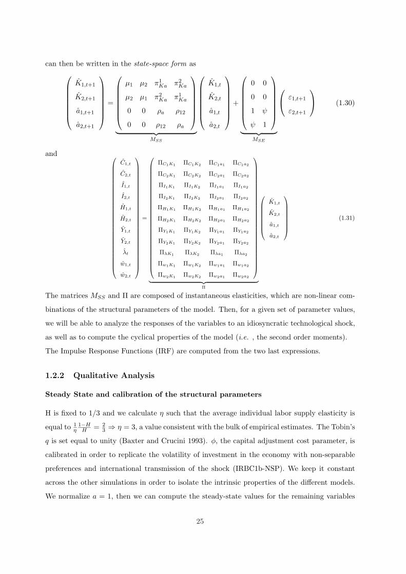
Figure 1.1: Separable preferences.
Ld
Ls
H
w
Instantaneous perturbation of the labor market equilibrium following a positive productivity shock.
The intertemporal wealth and substitution effects are captured by the term Ci,t. That is,
the labor supply depends on the household’s consumption behavior (see figure 1.1). With
the benchmark calibration, the substitution effects predominate, which explains the positive
response of labor at impact (figure 1.2).
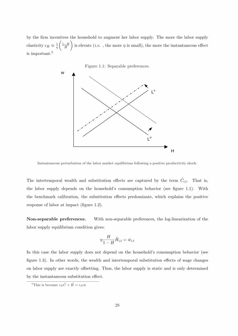
Non-separable preferences. With non-separable preferences, the log-linearization of the
labor supply equilibrium condition gives:
ηH
1−HHi,t = wi,t
In this case the labor supply does not depend on the household’s consumption behavior (see
figure 1.3). In other words, the wealth and intertemporal substitution effects of wage changes
on labor supply are exactly offsetting. Thus, the labor supply is static and is only determined
by the instantaneous substitution effect.
5This is because εHC + H = εHw.
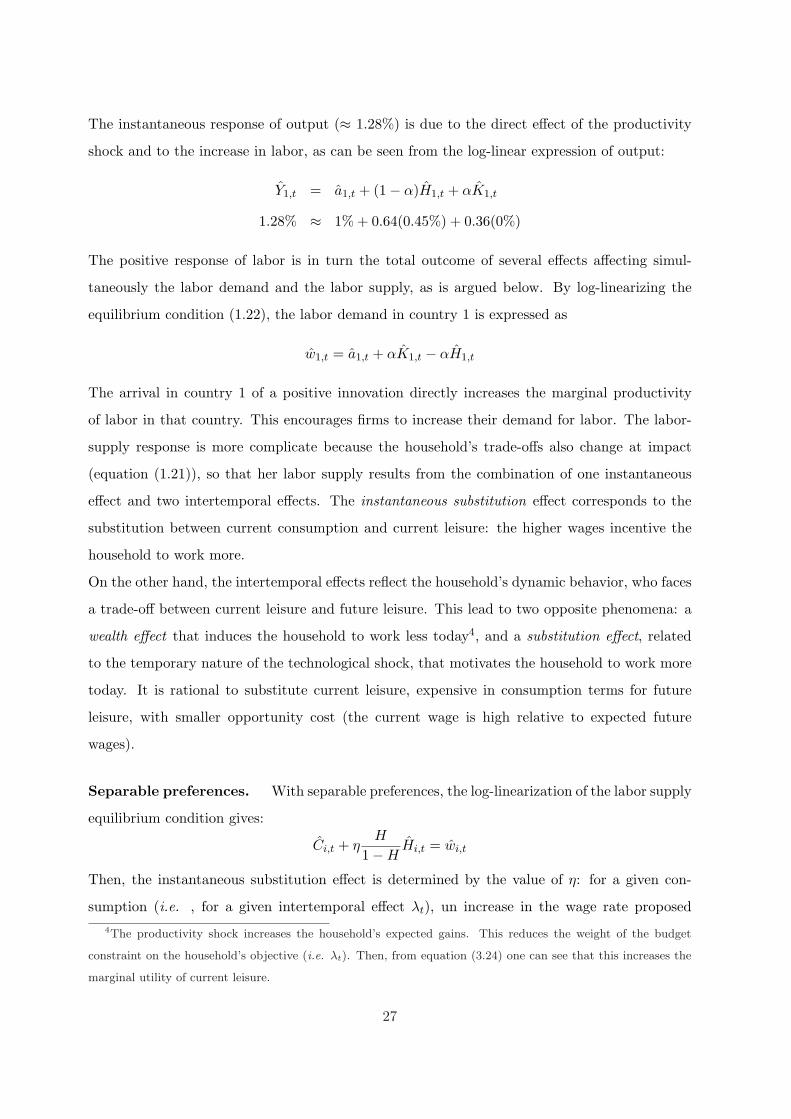
28
Figure 1.2: IRF - IRBCa-SP (benchmark)
0 50 1000
0.05
0.1
0.15
0.2
0.25C
1C
2
0 50 100−0.2
−0.1
0
0.1
0.2
0.3
0.4
0.5H
1H
2
0 50 100−0.5
0
0.5
1
1.5Y
1Y
2
0 50 100−2
0
2
4
6I1I2
0 50 1000
0.2
0.4
0.6
0.8
1W
1W
2
0 50 100−5
−4
−3
−2
−1
0
1
2NX
1NX
2
Figure 1.3: Non-separable preferences.
Ld
Ls
H
w
Instantaneous perturbation of the labor market equilibrium following a positive productivity shock.
29
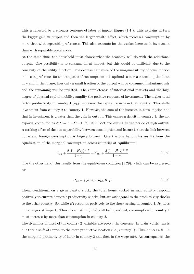
This is reflected by a stronger response of labor at impact (figure (1.4)). This explains in turn
the bigger gain in output and then the larger wealth effect, which increases consumption by
more than with separable preferences. This also accounts for the weaker increase in investment
than with separable preferences.
At the same time, the household must choose what the economy will do with the additional
output. One possibility is to consume all at impact, but this would be inefficient due to the
concavity of the utility function. The decreasing nature of the marginal utility of consumption
induces a preference for smooth paths of consumption: it is optimal to increase consumption both
now and in the future, thus only a small fraction of the output will be consumed instantaneously
and the remaining will be invested. The completeness of international markets and the high
degree of physical capital mobility amplify the positive response of investment. The higher total
factor productivity in country 1 (a1,t) increases the capital returns in that country. This shifts
investment from country 2 to country 1. However, the sum of the increase in consumption and
that in investment is greater than the gain in output. This causes a deficit in country 1: the net
exports, computed as NX = Y −C − I, fall at impact and during all the period of high output.
A striking effect of the non-separability between consumption and leisure is that the link between
home and foreign consumption is largely broken. One the one hand, this results from the
equalization of the marginal consumption across countries at equilibrium:
C1,t +σ(1−H1,t)1−η
1− η= C2,t +
σ(1−H2,t)1−η
1− η(1.32)
One the other hand, this results from the equilibrium condition (1.29), which can be expressed
as:
Hi,t = f(α, σ, η, ai,t,Ki,t) (1.33)
Then, conditional on a given capital stock, the total hours worked in each country respond
positively to current domestic productivity shocks, but are orthogonal to the productivity shocks
to the other country. So, while H1 responds positively to the shock arising in country 1, H2 does
not changes at impact. Thus, to equation (1.32) still being verified, consumption in country 1
must increase by more than consumption in country 2.
The dynamics of most of the country 2 variables are pretty the converse. In plain words, this is
due to the shift of capital to the more productive location (i.e., country 1). This induces a fall in
the marginal productivity of labor in country 2 and then in the wage rate. As consequence, the
30
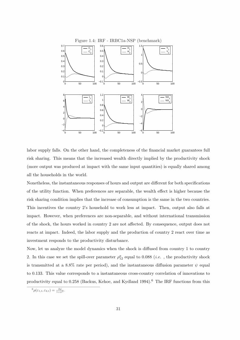
Figure 1.4: IRF - IRBC1a-NSP (benchmark)
0 50 1000
0.1
0.2
0.3
0.4
0.5
0.6
0.7C
1C
2
0 50 100−0.1
0
0.1
0.2
0.3
0.4
0.5
0.6H
1H
2
0 50 100−0.5
0
0.5
1
1.5Y
1Y
2
0 50 100−4
−2
0
2
4
6
8I1I2
0 50 100−0.2
0
0.2
0.4
0.6
0.8
1
1.2W
1W
2
0 50 100−6
−4
−2
0
2
4NX
1NX
2
labor supply falls. On the other hand, the completeness of the financial market guarantees full
risk sharing. This means that the increased wealth directly implied by the productivity shock
(more output was produced at impact with the same input quantities) is equally shared among
all the households in the world.
Nonetheless, the instantaneous responses of hours and output are different for both specifications
of the utility function. When preferences are separable, the wealth effect is higher because the
risk sharing condition implies that the increase of consumption is the same in the two countries.
This incentives the country 2’s household to work less at impact. Then, output also falls at
impact. However, when preferences are non-separable, and without international transmission
of the shock, the hours worked in country 2 are not affected. By consequence, output does not
reacts at impact. Indeed, the labor supply and the production of country 2 react over time as
investment responds to the productivity disturbance.
Now, let us analyze the model dynamics when the shock is diffused from country 1 to country
2. In this case we set the spill-over parameter ρa12 equal to 0.088 (i.e. , the productivity shock
is transmitted at a 8.8% rate per period), and the instantaneous diffusion parameter ψ equal
to 0.133. This value corresponds to a instantaneous cross-country correlation of innovations to
productivity equal to 0.258 (Backus, Kehoe, and Kydland 1994).6 The IRF functions from this
6ρ(ε1,t, ε2,t) = 2ψ1+ψ2 .
31
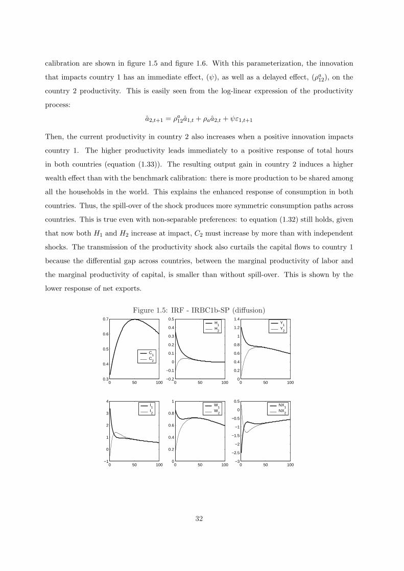
calibration are shown in figure 1.5 and figure 1.6. With this parameterization, the innovation
that impacts country 1 has an immediate effect, (ψ), as well as a delayed effect, (ρa12), on the
country 2 productivity. This is easily seen from the log-linear expression of the productivity
process:
a2,t+1 = ρa12a1,t + ρaa2,t + ψε1,t+1
Then, the current productivity in country 2 also increases when a positive innovation impacts
country 1. The higher productivity leads immediately to a positive response of total hours
in both countries (equation (1.33)). The resulting output gain in country 2 induces a higher
wealth effect than with the benchmark calibration: there is more production to be shared among
all the households in the world. This explains the enhanced response of consumption in both
countries. Thus, the spill-over of the shock produces more symmetric consumption paths across
countries. This is true even with non-separable preferences: to equation (1.32) still holds, given
that now both H1 and H2 increase at impact, C2 must increase by more than with independent
shocks. The transmission of the productivity shock also curtails the capital flows to country 1
because the differential gap across countries, between the marginal productivity of labor and
the marginal productivity of capital, is smaller than without spill-over. This is shown by the
lower response of net exports.
Figure 1.5: IRF - IRBC1b-SP (diffusion)
0 50 1000.3
0.4
0.5
0.6
0.7
C1
C2
0 50 100−0.2
−0.1
0
0.1
0.2
0.3
0.4
0.5H
1H
2
0 50 1000
0.2
0.4
0.6
0.8
1
1.2
1.4Y
1Y
2
0 50 100−1
0
1
2
3
4I1I2
0 50 1000
0.2
0.4
0.6
0.8
1W
1W
2
0 50 100−3
−2.5
−2
−1.5
−1
−0.5
0
0.5NX
1NX
2
32
Figure 1.6: IRF - IRBC1b-NSP (diffusion)
0 50 1000.4
0.5
0.6
0.7
0.8
0.9
C1
C2
0 50 1000
0.1
0.2
0.3
0.4
0.5
0.6
0.7H
1H
2
0 50 1000
0.2
0.4
0.6
0.8
1
1.2
1.4Y
1Y
2
0 50 100−2
−1
0
1
2
3
4I1I2
0 50 1000
0.2
0.4
0.6
0.8
1W
1W
2
0 50 100−4
−3
−2
−1
0
1
2NX
1NX
2
1.2.3 Quantitative Properties
The intuitions given by the IRF functions are reinforced by the results reported in table 1.2.
The non-separability of the utility function improves the model’s predictions regarding the in-
ternational comovements. For the benchmark calibration (columns 2 and 3 of table 1.2), the
cross-country correlation of outputs and total hours are less negative than with separable prefer-
ences. More strikingly, the cross-correlation of consumptions falls from 1 to 0.26. In both cases,
due to the high capital mobility and to the completeness of financial markets, investments are
negatively correlated.
Regarding the within-country statistics, we observe that the non-separability of the household’s
preferences augments the relative volatility of consumption and that of the total hours. Con-
versely, it diminishes the relative volatility of both investment and the labor productivity, but
the persistence of the variables still virtually unchanged.
Turning to the procyclicality of the variables, we remark that only the correlation of consumption
with output seems sensible to the specification of preferences. As is expected from the previous
analysis, this correlation is lower with separable preferences. Finally, as soon as the shock is
transmitted (last two columns of table 1.2), the cross-country correlations of output and labor
input increase. However, this largely increases the cross-correlation of consumptions (from 0.26
to 0.84).
33
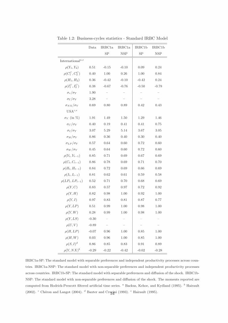
Table 1.2: Business-cycles statistics - Standard IRBC Model
Data IRBC1a IRBC1a IRBC1b IRBC1b
SP NSP SP NSP
Internationala,e
ρ(Y1, Y2) 0.51 -0.15 -0.10 0.09 0.24
ρ(CC1 , CC
2 ) 0.40 1.00 0.26 1.00 0.84
ρ(H1, H2) 0.36 -0.42 -0.10 -0.42 0.24
ρ(IC1 , IC
2 ) 0.38 -0.67 -0.76 -0.50 -0.78
στ/σY 1.90 – – – –
σΓ/σY 3.28 – – – –
σNX/σY 0.69 0.80 0.89 0.42 0.43
USAc,e
σY (in %) 1.91 1.49 1.50 1.29 1.46
σC/σY 0.40 0.19 0.41 0.41 0.75
σI/σY 3.07 5.29 5.14 3.67 3.05
σH/σY 0.86 0.36 0.40 0.30 0.40
σLP /σY 0.57 0.64 0.60 0.72 0.60
σW /σY 0.45 0.64 0.60 0.72 0.60
ρ(Yt, Yt−1) 0.85 0.71 0.69 0.67 0.69
ρ(Ct, Ct−1) 0.86 0.78 0.69 0.71 0.70
ρ(Ht, Ht−1) 0.84 0.72 0.69 0.66 0.69
ρ(It, It−1) 0.81 0.62 0.61 0.59 0.58
ρ(LPt, LPt−1) 0.52 0.71 0.70 0.68 0.69
ρ(Y, C) 0.83 0.57 0.97 0.72 0.92
ρ(Y, H) 0.82 0.98 1.00 0.92 1.00
ρ(Y, I) 0.97 0.83 0.81 0.87 0.77
ρ(Y, LP ) 0.51 0.99 1.00 0.98 1.00
ρ(Y, W ) 0.28 0.99 1.00 0.98 1.00
ρ(Y, LS) -0.30 – – – –
ρ(U, V ) -0.89 – – – –
ρ(H, LP ) -0.07 0.96 1.00 0.85 1.00
ρ(H, W ) 0.03 0.96 1.00 0.85 1.00
ρ(S, I)d 0.86 0.85 0.83 0.91 0.89
ρ(Y, NX)b -0.29 -0.22 -0.42 -0.02 -0.28
IRBC1a-SP: The standard model with separable preferences and independent productivity processes across coun-
tries. IRBC1a-NSP: The standard model with non-separable preferences and independent productivity processes
across countries. IRBC1b-SP: The standard model with separable preferences and diffusion of the shock. IRBC1b-
NSP: The standard model with non-separable preferences and diffusion of the shock. The moments reported are
computed from Hodrick-Prescott filtered artificial time series. a Backus, Kehoe, and Kydland (1995). b Hairault
(2002). c Cheron and Langot (2004). d Baxter and Crucini (1993). e Hairault (1995).34
1.2.4 Sensibility analysis
To complete the analysis, in this subsection we conduct a sensibility analysis of variations in
two key parameters of the model: η, that determines the labor supply elasticity, and φ, the
parameter governing the capital adjustment costs. In particular, the first case can be though
off as a test over the agents preferences. Whereas the second test is conducted just to assess the
role of this new parameter with respect to the canonical closed-economy framework.
Separable preferences
Sensibility to changes in η (εH). From Table 1.3 we can see that as long as the elasticity
of labor εH increases, the cross-country correlation of outputs, investments and total hours falls,
whereas the cross correlation of consumptions still equal to one. The standard deviation of
output, total hours and investment increases. By contrast, the standard deviation of consump-
tion and that of the labor productivity fall. The persistence and the procyclicality still roughly
unchanged but the correlation of labor productivity with both the total hours and output falls.
For a better understanding of these results we also analyze the changes on the instantaneous
elasticities. Particularly, we concentrate on the third column of the Π matrix in equation 1.31,
which captures the direct effect of the productivity shock to country 1 (Table A.1). As we can
see, the response of all the country 1 variables increases as εH increases, apart from the real
wage (see the log-linear expressions of the labor supply). The converse is true for the country 2
variables, consumption excepted.
Sensibility to changes in φ. As we can see from Table A.3, when φ increases, the response
of investment is lower in country 1 but higher in country 2, so that the gap between them
becomes smaller. This leads to larger cross-country correlation of investments. Finally, the
response of total hours is decreasing in φ for both countries, whereas the response of the labor
productivity increases.
Non-separable preferences
Sensibility to changes in η (εH). The most striking differences with what happens with
separable preferences, are the lower cross-country correlation of consumption and the equaliza-
tion between the cross-country correlation of total hours and the one of outputs. This comes
from the insensibility of H2 and Y2 to the productivity shock to country 1 (Table A.2). In
35

addition, the correlation of output with both total hours and labor productivity, as well as the
correlation of total hours with labor productivity, are all equal to 1.
Sensibility to changes in φ. The cross-country correlations increase as the adjustment
costs become larger. This is remarkable for investment. The relative volatility of both total
hours and labor productivity does not change. This is explained by the insensibility of their
instantaneous elasticities to changes in φ (Table A.3).
1.3 Conclusions
The canonical IRBC model developed in this chapter appears to be insufficient to account for
most of the international features of business cycles. Moreover, it has the same limitations as
its closed-economy counterpart regarding the dynamics of the real wage, the labor productivity
and the total hours. In addition, due to its single-good nature, the model is obviously silent
concerning the international facts involving relative prices. Nonetheless, we can point out the
following:
Given a world economy composed of two symmetric countries which trade a single-homogeneous
good then,
• When productivity is identically and independently distributed both across time and
across countries, the non-separability between consumption and leisure induces a low
cross-country correlation of consumption and a negative cross-country correlation of hours
worked, investment and output.7
• As soon as we allow for positive international correlation of contemporaneous innovations
to productivity, the cross-country correlation of consumptions, hours worked and outputs
increase.
According to these results, chapter 2 exposes a survey of several standard amendments intended
to improve the predictions of the model.
7This is the particular case analyzed by Devereux, Gregory, and Smith (1992).
36
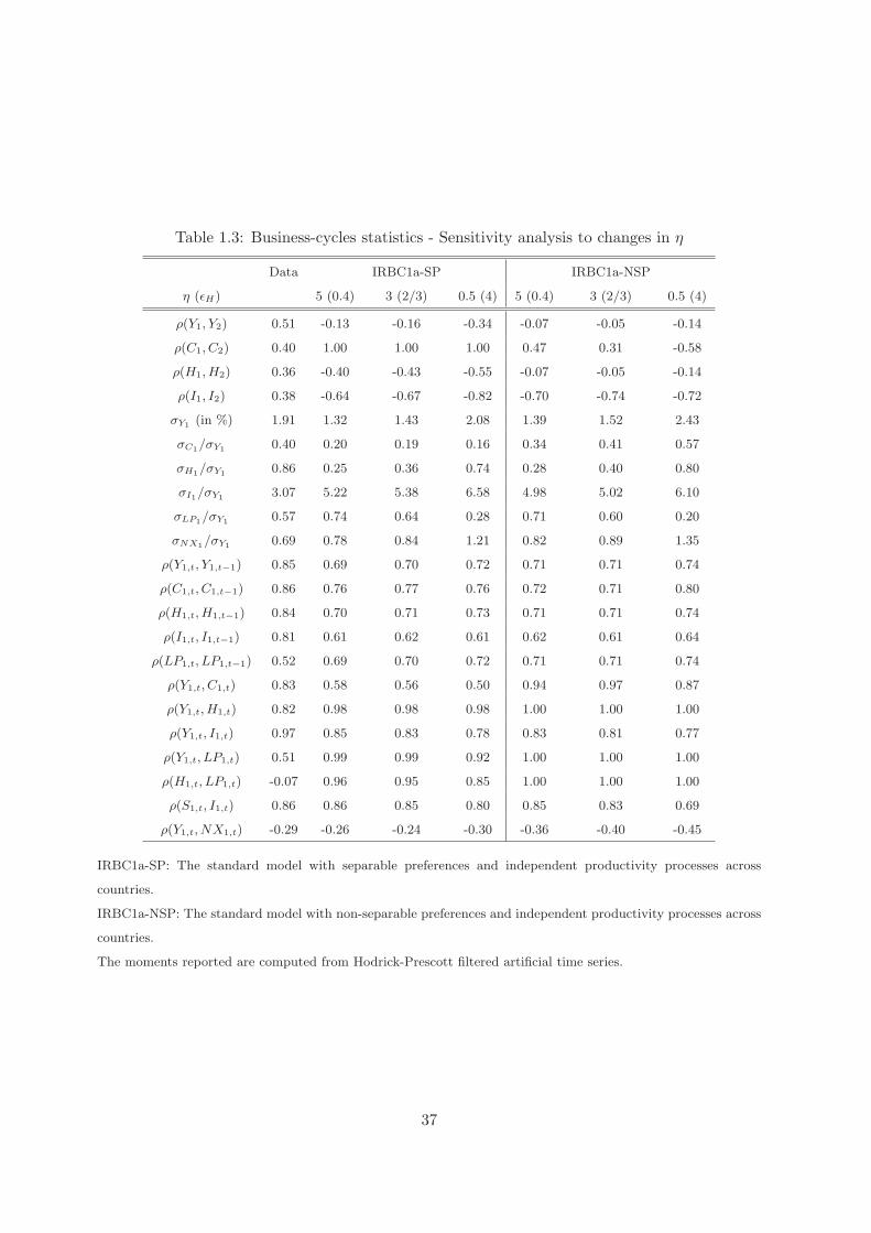
Table 1.3: Business-cycles statistics - Sensitivity analysis to changes in η
Data IRBC1a-SP IRBC1a-NSP
η (εH) 5 (0.4) 3 (2/3) 0.5 (4) 5 (0.4) 3 (2/3) 0.5 (4)
ρ(Y1, Y2) 0.51 -0.13 -0.16 -0.34 -0.07 -0.05 -0.14
ρ(C1, C2) 0.40 1.00 1.00 1.00 0.47 0.31 -0.58
ρ(H1, H2) 0.36 -0.40 -0.43 -0.55 -0.07 -0.05 -0.14
ρ(I1, I2) 0.38 -0.64 -0.67 -0.82 -0.70 -0.74 -0.72
σY1 (in %) 1.91 1.32 1.43 2.08 1.39 1.52 2.43
σC1/σY1 0.40 0.20 0.19 0.16 0.34 0.41 0.57
σH1/σY1 0.86 0.25 0.36 0.74 0.28 0.40 0.80
σI1/σY1 3.07 5.22 5.38 6.58 4.98 5.02 6.10
σLP1/σY1 0.57 0.74 0.64 0.28 0.71 0.60 0.20
σNX1/σY1 0.69 0.78 0.84 1.21 0.82 0.89 1.35
ρ(Y1,t, Y1,t−1) 0.85 0.69 0.70 0.72 0.71 0.71 0.74
ρ(C1,t, C1,t−1) 0.86 0.76 0.77 0.76 0.72 0.71 0.80
ρ(H1,t, H1,t−1) 0.84 0.70 0.71 0.73 0.71 0.71 0.74
ρ(I1,t, I1,t−1) 0.81 0.61 0.62 0.61 0.62 0.61 0.64
ρ(LP1,t, LP1,t−1) 0.52 0.69 0.70 0.72 0.71 0.71 0.74
ρ(Y1,t, C1,t) 0.83 0.58 0.56 0.50 0.94 0.97 0.87
ρ(Y1,t, H1,t) 0.82 0.98 0.98 0.98 1.00 1.00 1.00
ρ(Y1,t, I1,t) 0.97 0.85 0.83 0.78 0.83 0.81 0.77
ρ(Y1,t, LP1,t) 0.51 0.99 0.99 0.92 1.00 1.00 1.00
ρ(H1,t, LP1,t) -0.07 0.96 0.95 0.85 1.00 1.00 1.00
ρ(S1,t, I1,t) 0.86 0.86 0.85 0.80 0.85 0.83 0.69
ρ(Y1,t, NX1,t) -0.29 -0.26 -0.24 -0.30 -0.36 -0.40 -0.45
IRBC1a-SP: The standard model with separable preferences and independent productivity processes across
countries.
IRBC1a-NSP: The standard model with non-separable preferences and independent productivity processes across
countries.
The moments reported are computed from Hodrick-Prescott filtered artificial time series.
37
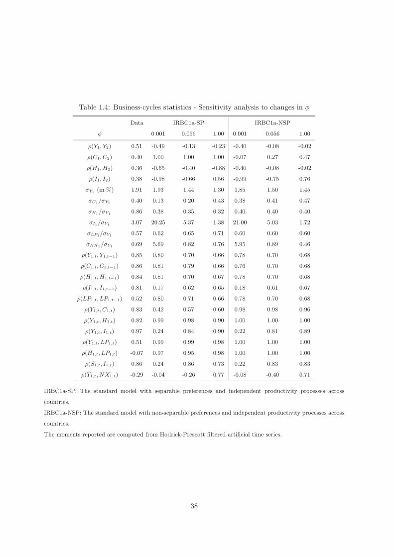
Table 1.4: Business-cycles statistics - Sensitivity analysis to changes in φ
Data IRBC1a-SP IRBC1a-NSP
φ 0.001 0.056 1.00 0.001 0.056 1.00
ρ(Y1, Y2) 0.51 -0.49 -0.13 -0.23 -0.40 -0.08 -0.02
ρ(C1, C2) 0.40 1.00 1.00 1.00 -0.07 0.27 0.47
ρ(H1, H2) 0.36 -0.65 -0.40 -0.88 -0.40 -0.08 -0.02
ρ(I1, I2) 0.38 -0.98 -0.66 0.56 -0.99 -0.75 0.76
σY1 (in %) 1.91 1.93 1.44 1.30 1.85 1.50 1.45
σC1/σY1 0.40 0.13 0.20 0.43 0.38 0.41 0.47
σH1/σY1 0.86 0.38 0.35 0.32 0.40 0.40 0.40
σI1/σY1 3.07 20.25 5.37 1.38 21.00 5.03 1.72
σLP1/σY1 0.57 0.62 0.65 0.71 0.60 0.60 0.60
σNX1/σY1 0.69 5.69 0.82 0.76 5.95 0.89 0.46
ρ(Y1,t, Y1,t−1) 0.85 0.80 0.70 0.66 0.78 0.70 0.68
ρ(C1,t, C1,t−1) 0.86 0.81 0.79 0.66 0.76 0.70 0.68
ρ(H1,t, H1,t−1) 0.84 0.81 0.70 0.67 0.78 0.70 0.68
ρ(I1,t, I1,t−1) 0.81 0.17 0.62 0.65 0.18 0.61 0.67
ρ(LP1,t, LP1,t−1) 0.52 0.80 0.71 0.66 0.78 0.70 0.68
ρ(Y1,t, C1,t) 0.83 0.42 0.57 0.60 0.98 0.98 0.96
ρ(Y1,t, H1,t) 0.82 0.99 0.98 0.90 1.00 1.00 1.00
ρ(Y1,t, I1,t) 0.97 0.24 0.84 0.90 0.22 0.81 0.89
ρ(Y1,t, LP1,t) 0.51 0.99 0.99 0.98 1.00 1.00 1.00
ρ(H1,t, LP1,t) -0.07 0.97 0.95 0.98 1.00 1.00 1.00
ρ(S1,t, I1,t) 0.86 0.24 0.86 0.73 0.22 0.83 0.83
ρ(Y1,t, NX1,t) -0.29 -0.04 -0.26 0.77 -0.08 -0.40 0.71
IRBC1a-SP: The standard model with separable preferences and independent productivity processes across
countries.
IRBC1a-NSP: The standard model with non-separable preferences and independent productivity processes across
countries.
The moments reported are computed from Hodrick-Prescott filtered artificial time series.
38

Chapter 2
A survey on international real
business cycles and the labor market
39
Introduction
In this chapter we review several standard extensions that were conceived to improve the pre-
dictions of the canonical model discussed in chapter 1. We still evaluate the performance of the
different economies with respect to the three puzzling facts early described, reproduced here for
easier reference. Two of them refer to observed international co-movements: (i) the cross corre-
lations for production, consumption, investment and labor input are positive across countries,
and (ii) the cross-correlation of consumptions tends to be lower than that of productions. The
last one concerns the observed rigidity of the real wage: (iii) the contemporaneous correlation
of the aggregate real wage with both output and labor input is very weak.
In stark contradiction, former international RBC models, as the one presented in chapter 1,
tends to predict negative cross-country correlations of labor input, investment and eventually
of output (Baxter 1995).1 Moreover, the theoretical correlation of consumptions is very close or
equal to unity, roughly two times than in the data.2
Nonetheless, as will be discussed along this chapter, posterior amendments have improved the
predictions of these canonical models. Basically by studying the mechanisms able either to
reduce the cross-correlation of consumptions, or to enhance the cyclical synchronization of pro-
ductions.3 On the other hand, one important weakness of RBC models for a closed economy is
the predicted high contemporaneous correlation of aggregate real wage with both output and
labor input, which contradicts the observed rigidity of the aggregate real wage.
In the first part of this chapter we survey three standard extensions of the basic walrasian
framework exposed in chapter 1. The first one aims to deep the link between the home and
the foreign countries. To this end we introduce an additional consumption/investment good by
considering national specialization (Backus, Kehoe, and Kydland 1994). This richer structure
adds a new mechanism by which the expansion of output experimented in the country receiving1To cite some examples: Arvanitis and Mikkola (1996), Baxter (1995), Baxter and Crucini (1993), Backus,
Kehoe, and Kydland (1994).2See, for instance, the seminal works of Backus, Kehoe, and Kydland (1992) and Baxter and Crucini (1993).3For instance, Devereux, Gregory, and Smith (1992) show that the non separability of consumption and leisure
in the agents’ preferences can generate a realistic international correlation between consumptions, while Stockman
and Tesar (1995) obtain similar results by incorporating non-traded goods and taste shocks. Baxter and Crucini
(1995) build a model with incomplete asset markets which, by reducing the incentive for risk sharing, improves
a little the correlation of consumptions. Kehoe and Perri (2000) almost solve the consumption-correlation puzzle
with a special incompleteness of financial markets in which each country may opt for the non-payment of his debt.
In this case, the country is excluded from financial markets and rests in autarky.
40
the shock, may induce an expansion of output in the other country. This potentially allows for
positive cross-correlations for labor inputs and investments.
This new mechanism pass through two channels. On the one side, agents demand a basket
of the two goods produced in the world for consumption and investment purposes. Then, the
additional wealth that results from a positive technological shock (that allows to produce more
with the same inputs), together with the perfect risk sharing, make agents of both countries to
increase their level of consumption at impact. This increases the demand for the two goods and
leads to an expansion of output in both countries. The other channel concerns the change in
the relative price of goods that follows the idiosyncratic innovation. Even if all this ameliorates
the theoretical predictions relative to the international facts, the model is far to be sufficient.
Following Galı (1994), we also distinguish the composite good for consumption from the com-
posite good for investment. However, this does not change the predictions of the model since
we allow for perfect competitive markets.
The second extension aims to reduce the international correlation of consumption. This is done
by restricting international trade to non-contingent bonds (Baxter 1995). This limitation in
the agent’s ability to risk pooling country-specific shocks produces more realistic international
correlations of outputs and consumptions. However, the correlation of outputs still larger than
the one of consumptions.
The last extension in the pure walrasian framework that we consider is the introduction of a
realistic potential for intra- and international capital flows by the disaggregation of the economy
into internationally traded and non-traded sectors (Stockman and Tesar 1995). This is justified
by the empirical evidence that roughly a half of the typical G-10 country’s output consists
of non-traded goods and services. It must be enhanced that, conversely to traditional IRBC
models with only technological shocks, as the Stockman and Tesar (1995)’s model, our model
predicts positive international input co-movements, which is more in accordance with empirical
correlations, but they are overstated particularly when shocks are highly persistent.
Nevertheless, because at this point we have not yet modified the walrasian nature of the labor
market, all models still fail in reproducing the fluctuations of the employment, the hours worked
and the real wage. Hence, the next step is to modify the walrasian labor market by introducing
search and matching in the labor market. This is the core of the second part of this survey,
in which we take as starting point the Hairault (2002)’s two-country, two-good search economy
to going ahead in the study of some stylized facts of the US labor market. Next, we make a
41

reduction to the single-good case to assess the role of each key hypotheses in the Hairault’s
economy. Namely, (i) the non-separability between consumption and leisure in the agents’
preferences, (ii) the existence of two goods in the world and so one relative price, and (iii) search
and bargaining in the labor market. In this single-good search framework we also evaluate
the predictions from the model with restricted international trade to non-contingent bonds.
However, we do not extend the search model to include two sectors because the results from the
walrasian economy are discouraging.
Regarding the search economies, we show that in the single-good economy, the combination of
search and matching in the labor market with the non-separability is enough to predict positive
comovements of labor inputs and investments as well as a large dissociation of consumptions.
Moreover, the procyclicality of real wage rate is reduced, and the correlation of total hours with
both output and labor productivity is low. Then, the three puzzles are partially solved. However,
consumptions correlation still larger than outputs correlation, even if the incompleteness of
financial markets produces more realistic international correlations of outputs and consumptions.
Then, we show that the gain from including two goods in that framework is that the model
is able now to replicate a correlation of outputs bigger than that of consumptions (Hairault
2002). However, the price dynamics provoked by a positive productivity shock decrease the
agent’s purchasing power, leading to a stronger vindication of salary and so to a slightly more
procyclical real wages.
2.1 National Specialization
The world economy consists of two countries (country 1 or home country and country 2 or foreign
country), each represented by a large number of identical consumers and a production technology.
Population size is normalized to unity. Each country specializes in the production of a single
good affected by persistent shocks A to productivity that are diffused internationally. Agents
demand constant elasticity of substitution (CES) baskets of the two goods for consumption C
and investment I purposes. Finally, the good produced in country 1 is taken as accounting unit.
2.1.1 Firms
Each country specializes in the production of a single good. The goods are produced with a
constant returns to scale technology using capital KCi , which is a composite of good 1 and good
42
2, and labor Hi as inputs,
Yi,t = ai,t(KCi,t)
αH1−αi,t (2.1)
As before, the variables ai,t stand for the stochastic component of the productivity variable
and follow the vector-autoregressive process described in the previous chapter. New capital
goods are internationally mobile and all investment is subject to quadratic adjustment costs:
Ci,t = φ2 (KC
i,t+1 −KCi,t)
2. Investment to country i = 1, 2 is a CES index of the two goods,
ICi,t =
[γ
1θII I
θI−1
θIi,t + (1− γI)
1θI I
θI−1
θIj 6=i,t
] θIθI−1
(2.2)
with the price index defined at each date as:
P Ii =
[γIP
1−θIi + (1− γI)P
1−θIj 6=i
] 11−θI
(2.3)
where θI denotes the elasticity of substitution between the national and the foreign goods when
they are used to production purposes, γI defines the share of the national good in the investment
basket, and Pi,t is the production price of good i. Capital accumulates over time according to
KCi,t+1 = (1− δ)KC
i,t + ICi,t (2.4)
The wage rate payed by firms is expressed in units of the national good (i.e. , firms pay a
“product wage”). Then, by normalizing the price of good 1 to P1,t = 1 ∀t, the dynamic problem
of each firm in country i = 1, 2 can be written, in units of the good 1 as follows:
W(KC1,t) = max
H1,t,IC1,t
Y1,t −PI
1,t(C1,t + IC1,t)− w1,tH1,t +
∫vtW(KC
1,t+1)dAt+1
(2.5)
W(KC2,t) = max
H2,t,IC2,t
ptY2,t − PI
2,t(C2,t + IC2,t)− ptw2,tH2,t +
∫vtW(KC
2,t+1)dAt+1
(2.6)
subject to constraints (2.1) and (2.4). In last expressions pt is the relative price of good 2 and
PIi,t ≡
P Ii,t
P1,t, and vt = v(At+1) stands for the firm’s actualization rate. The optimal demands for
labor and capital are then:
wi,t = (1− α)Yi,t
Hi,t, for i=1,2 (2.7)
qi,t ≡ PIi,t + PI
i,t
∂CCi,t
∂ICi,t
, for i=1,2 (2.8)
q1,t =∫
vt
(α
Y1,t+1
KC1,t+1
+ q1,t+1 − δPI1,t
)dAt+1, for i=1 (2.9)
q2,t =∫
vt
(αpt+1
Y2,t+1
KC2,t+1
+ q2,t+1 − δPI2,t
)dAt+1, for i=2 (2.10)
43

Finally, we impose the following transversality condition for capital, where qi,t is the shadow
price of capital:
limj→∞
Et[qi,t+j+1KCt+j+1] = 0 (2.11)
2.1.2 Households
Given the wage rate proposed by firms, the representative household’s objective is to choose a
contingency plan CCi,t,Hi,t that maximizes her expected lifetime utility
E0
∞∑
t=0
βtU(CCi,t, 1−Hi,t) (2.12)
CCi,t stands for the household’s consumption of the composite goods CC . Similar than investment,
consumption is assumed to have the following CES structure:
CCi =
[γ
1θCC C
θC−1
θCi + (1− γC)
1θC C
θC−1
θCj 6=i
] θCθC−1
(2.13)
with the price index defined as
PCi =
[γCP 1−θC
i + (1− γC)P 1−θCj 6=i
] 11−θC
(2.14)
where θC is the elasticity of substitution between the goods and γC the share of good 1 in the
consumption basket.
Financial markets are complete and we assume perfect international risk sharing: households in
the two countries have access to contingent claims Bi,t = Bi(At) at prices vt = v(At+1) providing
one unit of good 1 (i.e. , of the accounting unit) if the state A occurs at t + 1. The households’
budget constraints are then
PCi,tC
Ci,t +
∫vtP1,t+1Bi,t+1dAt+1 ≤ P1,tBi,t + Pi,twi,tHi,t (λi,t) (2.15)
which are written in terms of good 1 as:
PC1,tC
C1,t +
∫vtB1,t+1dAt+1 ≤ B1,t + w1,tH1,t (λ1,t) (2.16)
PC2,tC
C2,t +
∫vtB2,t+1dAt+1 ≤ B2,t + ptw2,tH2,t (λ2,t) (2.17)
with PCi,t ≡
P Ci,t
P1,t. Let f(A) ≡ f(At+1, At) denote the density function describing the transition
from the state At to the state At+1. Then, the representative household in country i = 1, 2
solves the dynamic problem:
V(Bi,t) = maxCC
i,t,Hi,t,Bi,t+1
U(CC
i,t, 1−Hi,t) + β
∫V(Bi,t+1)f(A)dA
(2.18)
44
subject to the respective budget constraint ((2.16) for i = 1, or (2.17) for i = 2).
If the agents’ preferences exhibit a standard separability between consumption and leisure,4 the
instantaneous utility is defined as:
U(CCi,t, 1−Hi,t) = log(CC
i,t) + σ(1−Hi,t)1−η
1− η, η > 0
and the optimality conditions are:
1CC
i,t
= PCi,tλi,t, for i=1,2 (2.19)
σ(1−H1,t)−ηPC1,tC
C1,t = w1,t, for i=1 (2.20)
σ(1−H2,t)−ηPC2,tC
C2,t = ptw2,t, for i=2 (2.21)
Then, with two imperfect-substitutable goods in the world, the separability hypothesis not longer
guarantees the equalization of consumptions among countries.
Else, if preferences exhibit a non-separability,5 the instantaneous utility is:
U(CCi,t, 1−Hi,t) = log
(Ci,t + σ
(1−Hi,t)1−η
1− η
), η > 0
which implies:
1
CCi,t + σ
(1−Hi,t)1−η
1−η
= PCi,tλi,t, for i=1,2 (2.22)
σ(1−H1,t)−ηPC1,t = w1,t, for i=1 (2.23)
σ(1−H2,t)−ηPC2,t = ptw2,t, for i=2 (2.24)
Either at odds with the predictions of the single-good economy, the non-separability combined
with the two-good hypothesis, is not longer helpful in disentangle national- from foreign con-
sumption.
Finally, the optimal choice of contingent bonds and the transversality condition are:
vt = βλi,t+1
λi,tf(A) (2.25)
limj→∞
Et[βt+jλi,t+jBi,t+j+1] = 0 (2.26)
With respect to the canonical model developed in chapter 1, the marginal utility of either
consumption and labor, is now affected by the evolution of prices, which react in turn to changes
in productivity.4See Chapter 1 for a detailed analysis of this kind of preferences.5Ibidem.
45
2.1.3 General Equilibrium
The equilibrium of this economy consists of a set of households’ optimal decision rules Ci(·),Hsi (·), Bi(·),
the firms’ optimal demands for capital and labor Kdi (·),Hd
i (·) and a set of prices pt,PCi,t,PI
i,t, wi,t, vt(At+1)equilibrating the goods market, the labor market and the financial market. Then, for each coun-
try:
Equilibrium on the Goods Market: The equilibrium on the goods market is given by
the accounting equations for output,6
Y1,t = C11,t + C2
1,t + I11,t + I2
1,t + C11,t + C2
1,t (2.27)
= γC
(PC1,t
)θC CC1,t + γI
(PI1,t
)θI IC1,t + (1− γC)
(PC2,t
)θC CC2,t + (1− γI)
(PI2,t
)θI (C2,t + IC2,t)
Y2,t = C12,t + C2
2,t + I12,t + I2
2,t + C12,t + C2
2,t (2.28)
= (1− γC)
(PC
1,t
pt
)θC
CC1,t + (1− γI)
(PI
1,t
pt
)θI
IC1,t + γC
(PC
2,t
pt
)θC
CC2,t + γI
(PI
2,t
pt
)θI
(IC2,t + C2,t)
κij,t, for κ = C, I, C stands for the demand for good j = 1, 2 from country i = 1, 2 for
consumption and investment purposes.
Equilibrium on the Labor Market: When preferences are separable, the desired hours
of work in each country are determined by the following conditions:
PC1,tC
C1,tσ(1−H1,t)−η = (1− α)
Y1,t
H1,t(2.29)
(PC2,t
pt
)CC
2,tσ(1−H2,t)−η = (1− α)Y2,t
H2,t(2.30)
and, either the following condition when preferences are non-separable:
PC1,tσ(1−H1,t)−η = (1− α)
Y1,t
H1,t(2.31)
(PC2,t
pt
)σ(1−H2,t)−η = (1− α)
Y2,t
H2,t(2.32)
The properties of these conditions are discussed in next section.
Equilibrium on the Financial and Capital Market: Equation (2.25) implies that the
initial wealth distribution in one country is proportional to the initial wealth distribution in the6See Annex B for details.
46
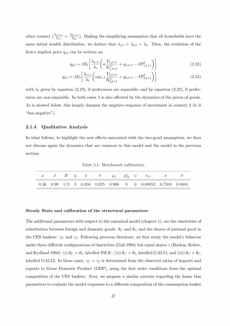
other country (λ1,t+1
λ1,t= λ2,t+1
λ2,t). Making the simplifying assumption that all households have the
same initial wealth distribution, we deduce that λ1,t = λ2,t = λt. Then, the evolution of the
firm’s implicit price qi,t can be written as:
q2,t = βEt
[λt+1
λt
(α
Y1,t+1
KC1,t+1
+ q1,t+1 − δPI1,t+1
)](2.33)
q2,t = βEt
[λt+1
λt
(αpt+1
Y2,t+1
KC2,t+1
+ q2,t+1 − δPI2,t+1
)](2.34)
with λt given by equation (2.19), if preferences are separable; and by equation (2.22), if prefer-
ences are non-separable. In both cases λ is also affected by the dynamics of the prices of goods.
As is showed below, this largely dampen the negative response of investment in country 2 (it is
“less negative”).
2.1.4 Qualitative Analysis
In what follows, to highlight the new effects associated with the two-good assumption, we does
not discuss again the dynamics that are common to this model and the model in the previous
section:
Table 2.1: Benchmark calibration.
α β H η φ δ ρa ρa12 ψ σεa σ σ
0.36 0.99 1/3 3 0.056 0.025 0.906 0 0 0.00852 0.7508 0.6804
Steady State and calibration of the structural parameters
The additional parameters with respect to the canonical model (chapter 1), are the elasticities of
substitution between foreign and domestic goods: θC and θI ; and the shares of national good in
the CES baskets: γC and γI . Following previous literature, we first study the model’s behavior
under three different configurations of elasticities (Galı 1994) but equal shares γ (Backus, Kehoe,
and Kydland 1994): (i) θC = θI , labelled BKK ; (ii) θC > θI , labelled GALI1; and (iii) θC < θI ,
labelled GALI2. In these cases, γC = γI is determined from the observed ratios of imports and
exports to Gross Domestic Product (GDP), using the first order conditions from the optimal
composition of the CES baskets. Next, we propose a similar exercise regarding the home bias
parameters to evaluate the model responses to a different composition of the consumption basket
47
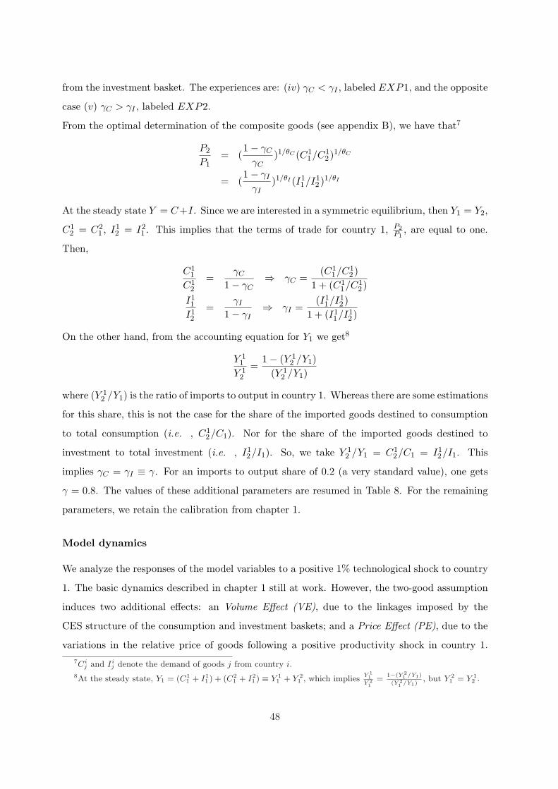
from the investment basket. The experiences are: (iv) γC < γI , labeled EXP1, and the opposite
case (v) γC > γI , labeled EXP2.
From the optimal determination of the composite goods (see appendix B), we have that7
P2
P1= (
1− γC
γC)1/θC (C1
1/C12 )1/θC
= (1− γI
γI)1/θI (I1
1/I12 )1/θI
At the steady state Y = C+I. Since we are interested in a symmetric equilibrium, then Y1 = Y2,
C12 = C2
1 , I12 = I2
1 . This implies that the terms of trade for country 1, P2P1
, are equal to one.
Then,
C11
C12
=γC
1− γC⇒ γC =
(C11/C1
2 )1 + (C1
1/C12 )
I11
I12
=γI
1− γI⇒ γI =
(I11/I1
2 )1 + (I1
1/I12 )
On the other hand, from the accounting equation for Y1 we get8
Y 11
Y 12
=1− (Y 1
2 /Y1)(Y 1
2 /Y1)
where (Y 12 /Y1) is the ratio of imports to output in country 1. Whereas there are some estimations
for this share, this is not the case for the share of the imported goods destined to consumption
to total consumption (i.e. , C12/C1). Nor for the share of the imported goods destined to
investment to total investment (i.e. , I12/I1). So, we take Y 1
2 /Y1 = C12/C1 = I1
2/I1. This
implies γC = γI ≡ γ. For an imports to output share of 0.2 (a very standard value), one gets
γ = 0.8. The values of these additional parameters are resumed in Table 8. For the remaining
parameters, we retain the calibration from chapter 1.
Model dynamics
We analyze the responses of the model variables to a positive 1% technological shock to country
1. The basic dynamics described in chapter 1 still at work. However, the two-good assumption
induces two additional effects: an Volume Effect (VE), due to the linkages imposed by the
CES structure of the consumption and investment baskets; and a Price Effect (PE), due to the
variations in the relative price of goods following a positive productivity shock in country 1.7Ci
j and Iij denote the demand of goods j from country i.
8At the steady state, Y1 = (C11 + I1
1 ) + (C21 + I2
1 ) ≡ Y 11 + Y 2
1 , which impliesY 11
Y 21
=1−(Y 2
1 /Y1)
(Y 21 /Y1)
, but Y 21 = Y 1
2 .
48
Table 2.2: Additional parameters
γC γI θC θI φ
BKK 0.8 0.8 1.5 1.5 0.1
GALI 1 0.8 0.8 1.75 0.79 0.1
GALI 2 0.8 0.8 0.6 5.4 0.1
EXP 1 0.6 0.8 0.6 5.4 0.1
EXP 2 0.8 0.6 0.6 5.4 0.1
The V E implies that, since γC 6= 1, the positive wealth effect induced by the shock itself makes
households in both countries to increase their demands for the two goods. In turn, the PE
modifies the real wage in country 2 via the deterioration of the terms of trade of country 1 (i.e.
pt).9
As in the canonical model, the household’s labor supply results from the combination of an
instantaneous substitution effect between current consumption and current leisure, and two
opposite intertemporal effects that reflect the household’s dynamic trade-off between current
leisure and future leisure. The total outcome is contingent on the parameterization of the
model and on the specification of the utility function. However, with respect to the single-good
canonical model, these new effects lead to quiet different dynamics for consumption and hours,
as it is discussed below.
Separable Preferences. The impulse response functions (IRF) following a technological
shock to country 1 are showed in figure 2.1 for the BKK calibration, in figure 2.2 for the GALI
calibrations, and in figure 2.3 for the own EXP calibrations (since we analyse the orthogonal
responses to the shock, we set the diffusion parameters to ψ = ρa12 = 0 to compute the IRF from
the model).
With separable preferences, the log-linearization of the labor supply equilibrium condition gives9That is, the higher productivity at impact in country 1 provokes a fall in the production price of good 1, and
thus an increase in pt.
49
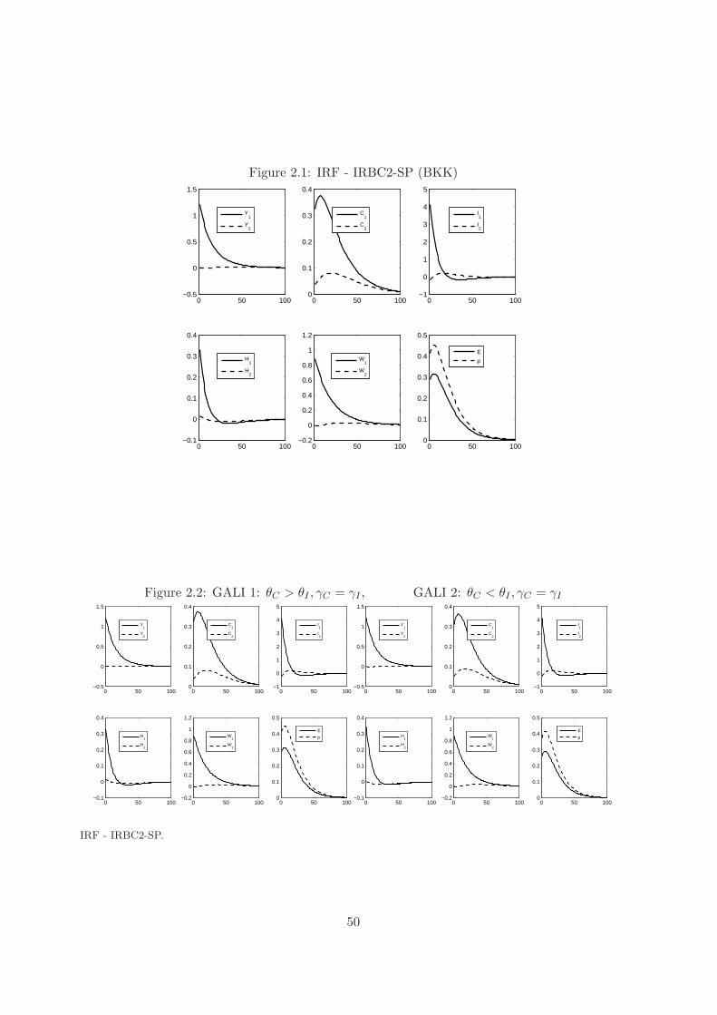
Figure 2.1: IRF - IRBC2-SP (BKK)
0 50 100−0.5
0
0.5
1
1.5
Y1
Y2
0 50 1000
0.1
0.2
0.3
0.4
C1
C2
0 50 100−1
0
1
2
3
4
5
I1
I2
0 50 100−0.1
0
0.1
0.2
0.3
0.4
H1
H2
0 50 100−0.2
0
0.2
0.4
0.6
0.8
1
1.2
W1
W2
0 50 1000
0.1
0.2
0.3
0.4
0.5
E
p
Figure 2.2: GALI 1: θC > θI , γC = γI , GALI 2: θC < θI , γC = γI
0 50 100−0.5
0
0.5
1
1.5
Y1
Y2
0 50 1000
0.1
0.2
0.3
0.4
C1
C2
0 50 100−1
0
1
2
3
4
5
I1
I2
0 50 100−0.1
0
0.1
0.2
0.3
0.4
H1
H2
0 50 100−0.2
0
0.2
0.4
0.6
0.8
1
1.2
W1
W2
0 50 1000
0.1
0.2
0.3
0.4
0.5
E
p
0 50 100−0.5
0
0.5
1
1.5
Y1
Y2
0 50 1000
0.1
0.2
0.3
0.4
C1
C2
0 50 100−1
0
1
2
3
4
5
I1
I2
0 50 100−0.1
0
0.1
0.2
0.3
0.4
H1
H2
0 50 100−0.2
0
0.2
0.4
0.6
0.8
1
1.2
W1
W2
0 50 1000
0.1
0.2
0.3
0.4
0.5
E
p
IRF - IRBC2-SP.
50
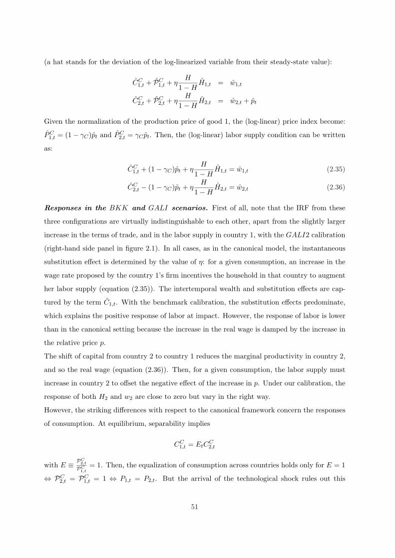
(a hat stands for the deviation of the log-linearized variable from their steady-state value):
CC1,t + PC
1,t + ηH
1−HH1,t = w1,t
CC2,t + PC
2,t + ηH
1−HH2,t = w2,t + pt
Given the normalization of the production price of good 1, the (log-linear) price index become:
PC1,t = (1− γC)pt and PC
2,t = γC pt. Then, the (log-linear) labor supply condition can be written
as:
CC1,t + (1− γC)pt + η
H
1−HH1,t = w1,t (2.35)
CC2,t − (1− γC)pt + η
H
1−HH2,t = w2,t (2.36)
Responses in the BKK and GALI scenarios. First of all, note that the IRF from these
three configurations are virtually indistinguishable to each other, apart from the slightly larger
increase in the terms of trade, and in the labor supply in country 1, with the GALI2 calibration
(right-hand side panel in figure 2.1). In all cases, as in the canonical model, the instantaneous
substitution effect is determined by the value of η: for a given consumption, an increase in the
wage rate proposed by the country 1’s firm incentives the household in that country to augment
her labor supply (equation (2.35)). The intertemporal wealth and substitution effects are cap-
tured by the term C1,t. With the benchmark calibration, the substitution effects predominate,
which explains the positive response of labor at impact. However, the response of labor is lower
than in the canonical setting because the increase in the real wage is damped by the increase in
the relative price p.
The shift of capital from country 2 to country 1 reduces the marginal productivity in country 2,
and so the real wage (equation (2.36)). Then, for a given consumption, the labor supply must
increase in country 2 to offset the negative effect of the increase in p. Under our calibration, the
response of both H2 and w2 are close to zero but vary in the right way.
However, the striking differences with respect to the canonical framework concern the responses
of consumption. At equilibrium, separability implies
CC1,t = EtC
C2,t
with E ≡ PC2,t
PC1,t
= 1. Then, the equalization of consumption across countries holds only for E = 1
⇔ PC2,t = PC
1,t = 1 ⇔ P1,t = P2,t. But the arrival of the technological shock rules out this
51
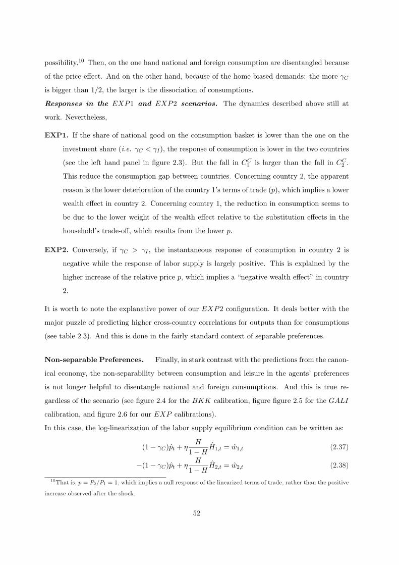
possibility.10 Then, on the one hand national and foreign consumption are disentangled because
of the price effect. And on the other hand, because of the home-biased demands: the more γC
is bigger than 1/2, the larger is the dissociation of consumptions.
Responses in the EXP1 and EXP2 scenarios. The dynamics described above still at
work. Nevertheless,
EXP1. If the share of national good on the consumption basket is lower than the one on the
investment share (i.e. γC < γI), the response of consumption is lower in the two countries
(see the left hand panel in figure 2.3). But the fall in CC1 is larger than the fall in CC
2 .
This reduce the consumption gap between countries. Concerning country 2, the apparent
reason is the lower deterioration of the country 1’s terms of trade (p), which implies a lower
wealth effect in country 2. Concerning country 1, the reduction in consumption seems to
be due to the lower weight of the wealth effect relative to the substitution effects in the
household’s trade-off, which results from the lower p.
EXP2. Conversely, if γC > γI , the instantaneous response of consumption in country 2 is
negative while the response of labor supply is largely positive. This is explained by the
higher increase of the relative price p, which implies a “negative wealth effect” in country
2.
It is worth to note the explanative power of our EXP2 configuration. It deals better with the
major puzzle of predicting higher cross-country correlations for outputs than for consumptions
(see table 2.3). And this is done in the fairly standard context of separable preferences.
Non-separable Preferences. Finally, in stark contrast with the predictions from the canon-
ical economy, the non-separability between consumption and leisure in the agents’ preferences
is not longer helpful to disentangle national and foreign consumptions. And this is true re-
gardless of the scenario (see figure 2.4 for the BKK calibration, figure figure 2.5 for the GALI
calibration, and figure 2.6 for our EXP calibrations).
In this case, the log-linearization of the labor supply equilibrium condition can be written as:
(1− γC)pt + ηH
1−HH1,t = w1,t (2.37)
−(1− γC)pt + ηH
1−HH2,t = w2,t (2.38)
10That is, p = P2/P1 = 1, which implies a null response of the linearized terms of trade, rather than the positive
increase observed after the shock.
52
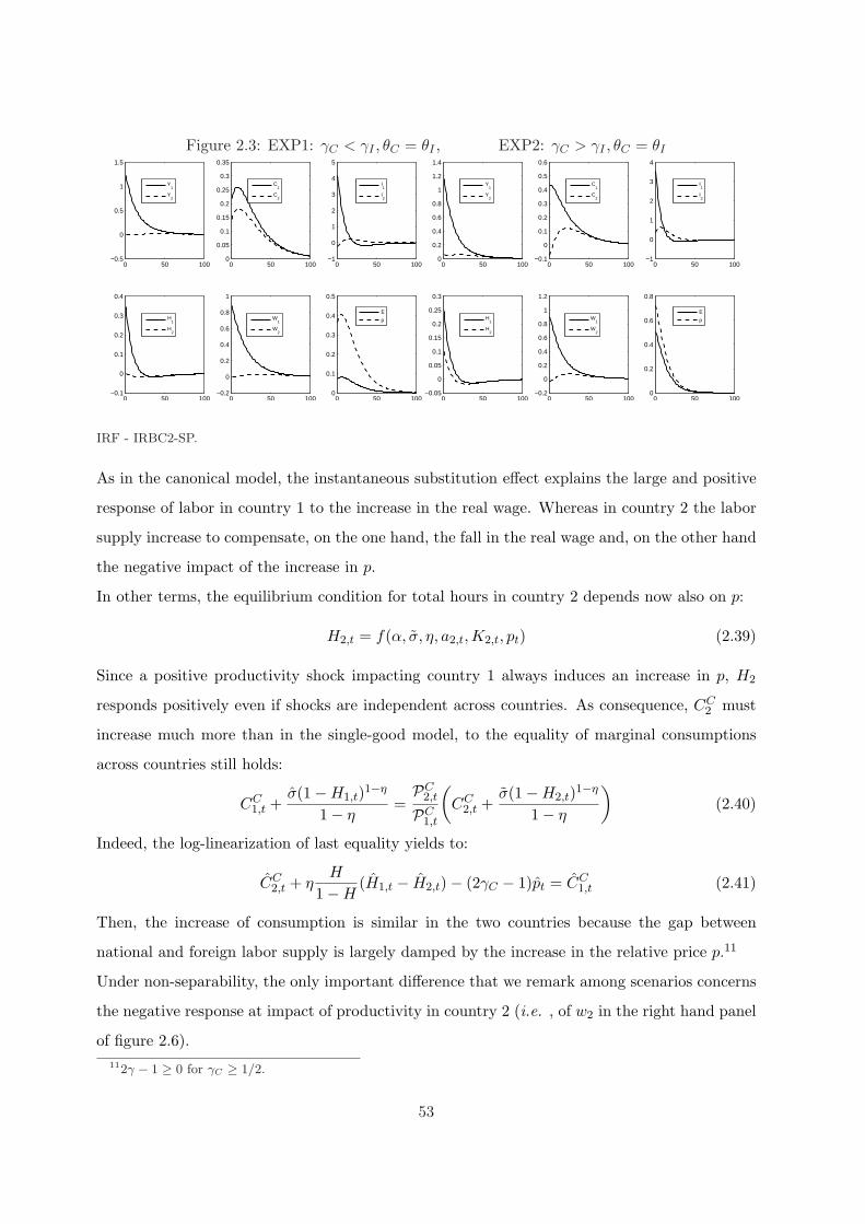
Figure 2.3: EXP1: γC < γI , θC = θI , EXP2: γC > γI , θC = θI
0 50 100−0.5
0
0.5
1
1.5
Y1
Y2
0 50 1000
0.05
0.1
0.15
0.2
0.25
0.3
0.35
C1
C2
0 50 100−1
0
1
2
3
4
5
I1
I2
0 50 100−0.1
0
0.1
0.2
0.3
0.4
H1
H2
0 50 100−0.2
0
0.2
0.4
0.6
0.8
1
W1
W2
0 50 1000
0.1
0.2
0.3
0.4
0.5
E
p
0 50 1000
0.2
0.4
0.6
0.8
1
1.2
1.4
Y1
Y2
0 50 100−0.1
0
0.1
0.2
0.3
0.4
0.5
0.6
C1
C2
0 50 100−1
0
1
2
3
4
I1
I2
0 50 100−0.05
0
0.05
0.1
0.15
0.2
0.25
0.3
H1
H2
0 50 100−0.2
0
0.2
0.4
0.6
0.8
1
1.2
W1
W2
0 50 1000
0.2
0.4
0.6
0.8
E
p
IRF - IRBC2-SP.
As in the canonical model, the instantaneous substitution effect explains the large and positive
response of labor in country 1 to the increase in the real wage. Whereas in country 2 the labor
supply increase to compensate, on the one hand, the fall in the real wage and, on the other hand
the negative impact of the increase in p.
In other terms, the equilibrium condition for total hours in country 2 depends now also on p:
H2,t = f(α, σ, η, a2,t,K2,t, pt) (2.39)
Since a positive productivity shock impacting country 1 always induces an increase in p, H2
responds positively even if shocks are independent across countries. As consequence, CC2 must
increase much more than in the single-good model, to the equality of marginal consumptions
across countries still holds:
CC1,t +
σ(1−H1,t)1−η
1− η=PC
2,t
PC1,t
(CC
2,t +σ(1−H2,t)1−η
1− η
)(2.40)
Indeed, the log-linearization of last equality yields to:
CC2,t + η
H
1−H(H1,t − H2,t)− (2γC − 1)pt = CC
1,t (2.41)
Then, the increase of consumption is similar in the two countries because the gap between
national and foreign labor supply is largely damped by the increase in the relative price p.11
Under non-separability, the only important difference that we remark among scenarios concerns
the negative response at impact of productivity in country 2 (i.e. , of w2 in the right hand panel
of figure 2.6).112γ − 1 ≥ 0 for γC ≥ 1/2.
53
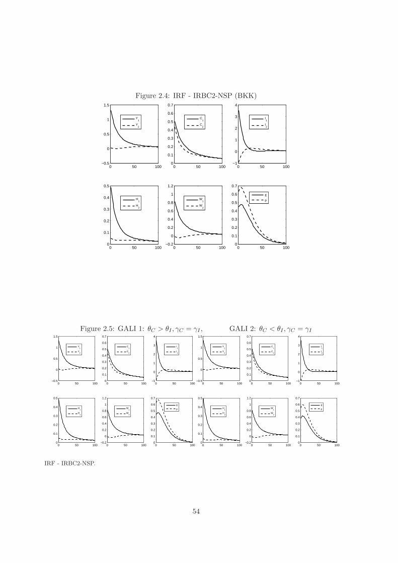
Figure 2.4: IRF - IRBC2-NSP (BKK)
0 50 100−0.5
0
0.5
1
1.5
Y1
Y2
0 50 1000
0.1
0.2
0.3
0.4
0.5
0.6
0.7
C1
C2
0 50 100−1
0
1
2
3
4
I1
I2
0 50 1000
0.1
0.2
0.3
0.4
0.5
H1
H2
0 50 100−0.2
0
0.2
0.4
0.6
0.8
1
1.2
W1
W2
0 50 1000
0.1
0.2
0.3
0.4
0.5
0.6
0.7
E
p
Figure 2.5: GALI 1: θC > θI , γC = γI , GALI 2: θC < θI , γC = γI
0 50 100−0.5
0
0.5
1
1.5
Y1
Y2
0 50 1000
0.1
0.2
0.3
0.4
0.5
0.6
0.7
C1
C2
0 50 100−1
0
1
2
3
4
I1
I2
0 50 1000
0.1
0.2
0.3
0.4
0.5
H1
H2
0 50 100−0.2
0
0.2
0.4
0.6
0.8
1
1.2
W1
W2
0 50 1000
0.1
0.2
0.3
0.4
0.5
0.6
0.7
E
p
0 50 100−0.5
0
0.5
1
1.5
Y1
Y2
0 50 1000
0.1
0.2
0.3
0.4
0.5
0.6
0.7
C1
C2
0 50 100−1
0
1
2
3
4
I1
I2
0 50 1000
0.1
0.2
0.3
0.4
0.5
H1
H2
0 50 100−0.2
0
0.2
0.4
0.6
0.8
1
1.2
W1
W2
0 50 1000
0.1
0.2
0.3
0.4
0.5
0.6
0.7
E
p
IRF - IRBC2-NSP.
54
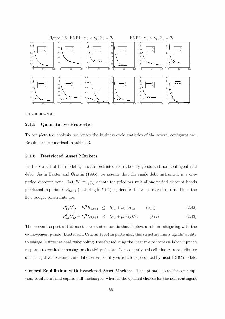
Figure 2.6: EXP1: γC < γI , θC = θI , EXP2: γC > γI , θC = θI
0 50 1000
0.2
0.4
0.6
0.8
1
1.2
1.4
Y1
Y2
0 50 1000
0.1
0.2
0.3
0.4
0.5
C1
C2
0 50 100−1
0
1
2
3
4
I1
I2
0 50 1000
0.1
0.2
0.3
0.4
0.5
H1
H2
0 50 100−0.2
0
0.2
0.4
0.6
0.8
1
1.2
W1
W2
0 50 1000
0.1
0.2
0.3
0.4
0.5
E
p
0 50 1000
0.2
0.4
0.6
0.8
1
1.2
1.4
Y1
Y2
0 50 1000
0.1
0.2
0.3
0.4
0.5
0.6
0.7
C1
C2
0 50 100−0.5
0
0.5
1
1.5
2
2.5
3
I1
I2
0 50 1000
0.1
0.2
0.3
0.4
0.5
H1
H2
0 50 100−0.2
0
0.2
0.4
0.6
0.8
1
1.2
W1
W2
0 50 1000
0.2
0.4
0.6
0.8
1
1.2
1.4
E
p
IRF - IRBC2-NSP.
2.1.5 Quantitative Properties
To complete the analysis, we report the business cycle statistics of the several configurations.
Results are summarized in table 2.3.
2.1.6 Restricted Asset Markets
In this variant of the model agents are restricted to trade only goods and non-contingent real
debt. As in Baxter and Crucini (1995), we assume that the single debt instrument is a one-
period discount bond. Let PBt ≡ 1
1+rtdenote the price per unit of one-period discount bonds
purchased in period t, Bi,t+1 (maturing in t + 1). rt denotes the world rate of return. Then, the
flow budget constraints are:
PC1,tC
C1,t + PB
t B1,t+1 ≤ B1,t + w1,tH1,t (λ1,t) (2.42)
PC2,tC
C2,t + PB
t B2,t+1 ≤ B2,t + ptw2,tH2,t (λ2,t) (2.43)
The relevant aspect of this asset market structure is that it plays a role in mitigating with the
co-movement puzzle (Baxter and Crucini 1995) In particular, this structure limits agents’ ability
to engage in international risk-pooling, thereby reducing the incentive to increase labor input in
response to wealth-increasing productivity shocks. Consequently, this eliminates a contributor
of the negative investment and labor cross-country correlations predicted by most IRBC models.
General Equilibrium with Restricted Asset Markets The optimal choices for consump-
tion, total hours and capital still unchanged, whereas the optimal choices for the non-contingent
55
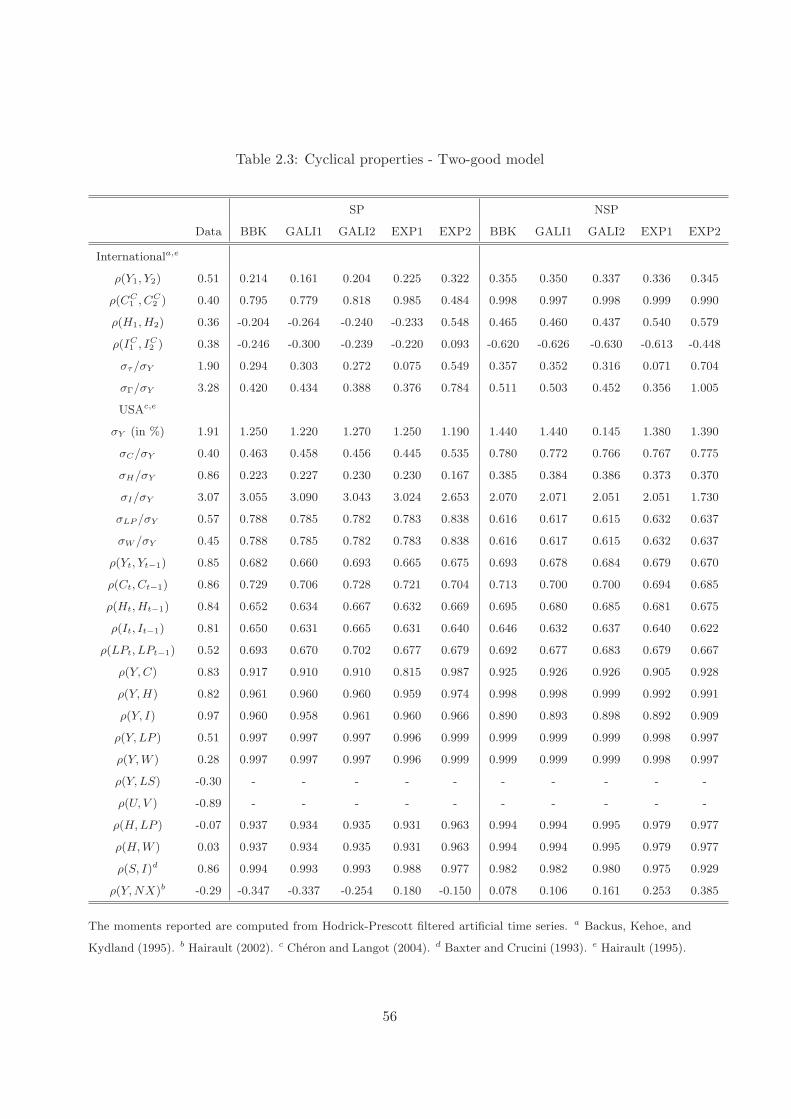
Table 2.3: Cyclical properties - Two-good model
SP NSP
Data BBK GALI1 GALI2 EXP1 EXP2 BBK GALI1 GALI2 EXP1 EXP2
Internationala,e
ρ(Y1, Y2) 0.51 0.214 0.161 0.204 0.225 0.322 0.355 0.350 0.337 0.336 0.345
ρ(CC1 , CC
2 ) 0.40 0.795 0.779 0.818 0.985 0.484 0.998 0.997 0.998 0.999 0.990
ρ(H1, H2) 0.36 -0.204 -0.264 -0.240 -0.233 0.548 0.465 0.460 0.437 0.540 0.579
ρ(IC1 , IC
2 ) 0.38 -0.246 -0.300 -0.239 -0.220 0.093 -0.620 -0.626 -0.630 -0.613 -0.448
στ/σY 1.90 0.294 0.303 0.272 0.075 0.549 0.357 0.352 0.316 0.071 0.704
σΓ/σY 3.28 0.420 0.434 0.388 0.376 0.784 0.511 0.503 0.452 0.356 1.005
USAc,e
σY (in %) 1.91 1.250 1.220 1.270 1.250 1.190 1.440 1.440 0.145 1.380 1.390
σC/σY 0.40 0.463 0.458 0.456 0.445 0.535 0.780 0.772 0.766 0.767 0.775
σH/σY 0.86 0.223 0.227 0.230 0.230 0.167 0.385 0.384 0.386 0.373 0.370
σI/σY 3.07 3.055 3.090 3.043 3.024 2.653 2.070 2.071 2.051 2.051 1.730
σLP /σY 0.57 0.788 0.785 0.782 0.783 0.838 0.616 0.617 0.615 0.632 0.637
σW /σY 0.45 0.788 0.785 0.782 0.783 0.838 0.616 0.617 0.615 0.632 0.637
ρ(Yt, Yt−1) 0.85 0.682 0.660 0.693 0.665 0.675 0.693 0.678 0.684 0.679 0.670
ρ(Ct, Ct−1) 0.86 0.729 0.706 0.728 0.721 0.704 0.713 0.700 0.700 0.694 0.685
ρ(Ht, Ht−1) 0.84 0.652 0.634 0.667 0.632 0.669 0.695 0.680 0.685 0.681 0.675
ρ(It, It−1) 0.81 0.650 0.631 0.665 0.631 0.640 0.646 0.632 0.637 0.640 0.622
ρ(LPt, LPt−1) 0.52 0.693 0.670 0.702 0.677 0.679 0.692 0.677 0.683 0.679 0.667
ρ(Y, C) 0.83 0.917 0.910 0.910 0.815 0.987 0.925 0.926 0.926 0.905 0.928
ρ(Y, H) 0.82 0.961 0.960 0.960 0.959 0.974 0.998 0.998 0.999 0.992 0.991
ρ(Y, I) 0.97 0.960 0.958 0.961 0.960 0.966 0.890 0.893 0.898 0.892 0.909
ρ(Y, LP ) 0.51 0.997 0.997 0.997 0.996 0.999 0.999 0.999 0.999 0.998 0.997
ρ(Y, W ) 0.28 0.997 0.997 0.997 0.996 0.999 0.999 0.999 0.999 0.998 0.997
ρ(Y, LS) -0.30 - - - - - - - - - -
ρ(U, V ) -0.89 - - - - - - - - - -
ρ(H, LP ) -0.07 0.937 0.934 0.935 0.931 0.963 0.994 0.994 0.995 0.979 0.977
ρ(H, W ) 0.03 0.937 0.934 0.935 0.931 0.963 0.994 0.994 0.995 0.979 0.977
ρ(S, I)d 0.86 0.994 0.993 0.993 0.988 0.977 0.982 0.982 0.980 0.975 0.929
ρ(Y, NX)b -0.29 -0.347 -0.337 -0.254 0.180 -0.150 0.078 0.106 0.161 0.253 0.385
The moments reported are computed from Hodrick-Prescott filtered artificial time series. a Backus, Kehoe, and
Kydland (1995). b Hairault (2002). c Cheron and Langot (2004). d Baxter and Crucini (1993). e Hairault (1995).
56
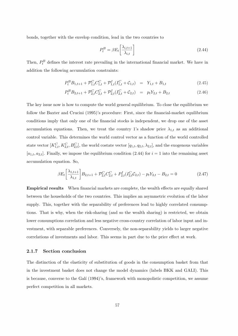
bonds, together with the envelop condition, lead in the two countries to
PBt = βEt
[λi,t+1
λi,t
](2.44)
Then, PBt defines the interest rate prevailing in the international financial market. We have in
addition the following accumulation constraints:
PBt B1,t+1 + PC
1,tCC1,t + PI
1,t(IC1,t + C1,t) = Y1,t + B1,t (2.45)
PBt B2,t+1 + PC
2,tCC2,t + PI
2,t(IC2,t + C2,t) = ptY2,t + B2,t (2.46)
The key issue now is how to compute the world general equilibrium. To close the equilibrium we
follow the Baxter and Crucini (1995)’s procedure: First, since the financial-market equilibrium
conditions imply that only one of the financial stocks is independent, we drop one of the asset
accumulation equations. Then, we treat the country 1’s shadow price λ1,t as an additional
control variable. This determines the world control vector as a function of the world controlled
state vector [KC1,t,K
C2,t, B
C2,t], the world costate vector [q1,t, q2,t, λ2,t], and the exogenous variables
[a1,t, a2,t]. Finally, we impose the equilibrium condition (2.44) for i = 1 into the remaining asset
accumulation equation. So,
βEt
[λ1,t+1
λ1,t
]B2,t+1 + PC
2,tCC2,t + P I
2,t(IC2,tC2,t)− ptY2,t −B2,t = 0 (2.47)
Empirical results When financial markets are complete, the wealth effects are equally shared
between the households of the two countries. This implies an asymmetric evolution of the labor
supply. This, together with the separability of preferences lead to highly correlated consump-
tions. That is why, when the risk-sharing (and so the wealth sharing) is restricted, we obtain
lower consumptions correlation and less negative cross-country correlation of labor input and in-
vestment, with separable preferences. Conversely, the non-separability yields to larger negative
correlations of investments and labor. This seems in part due to the price effect at work.
2.1.7 Section conclusion
The distinction of the elasticity of substitution of goods in the consumption basket from that
in the investment basket does not change the model dynamics (labels BKK and GALI). This
is because, converse to the Galı (1994)’s, framework with monopolistic competition, we assume
perfect competition in all markets.
57
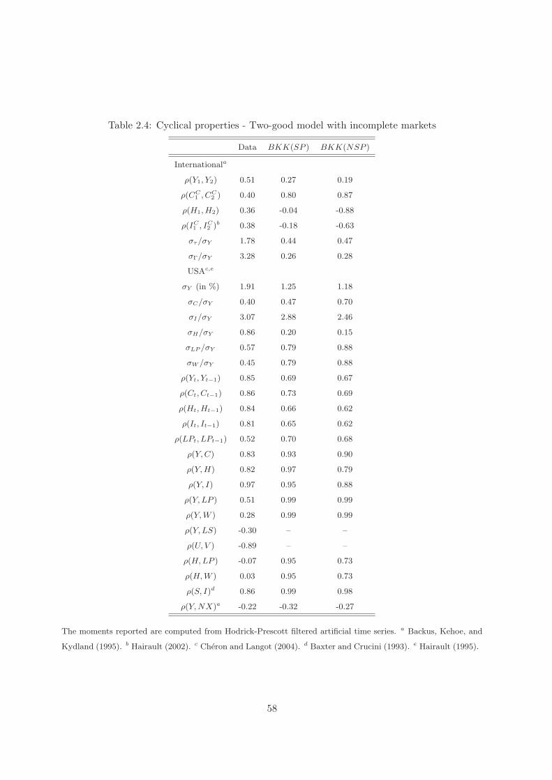
Table 2.4: Cyclical properties - Two-good model with incomplete markets
Data BKK(SP ) BKK(NSP )
Internationala
ρ(Y1, Y2) 0.51 0.27 0.19
ρ(CC1 , CC
2 ) 0.40 0.80 0.87
ρ(H1, H2) 0.36 -0.04 -0.88
ρ(IC1 , IC
2 )b 0.38 -0.18 -0.63
στ/σY 1.78 0.44 0.47
σΓ/σY 3.28 0.26 0.28
USAc,e
σY (in %) 1.91 1.25 1.18
σC/σY 0.40 0.47 0.70
σI/σY 3.07 2.88 2.46
σH/σY 0.86 0.20 0.15
σLP /σY 0.57 0.79 0.88
σW /σY 0.45 0.79 0.88
ρ(Yt, Yt−1) 0.85 0.69 0.67
ρ(Ct, Ct−1) 0.86 0.73 0.69
ρ(Ht, Ht−1) 0.84 0.66 0.62
ρ(It, It−1) 0.81 0.65 0.62
ρ(LPt, LPt−1) 0.52 0.70 0.68
ρ(Y, C) 0.83 0.93 0.90
ρ(Y, H) 0.82 0.97 0.79
ρ(Y, I) 0.97 0.95 0.88
ρ(Y, LP ) 0.51 0.99 0.99
ρ(Y, W ) 0.28 0.99 0.99
ρ(Y, LS) -0.30 – –
ρ(U, V ) -0.89 – –
ρ(H, LP ) -0.07 0.95 0.73
ρ(H, W ) 0.03 0.95 0.73
ρ(S, I)d 0.86 0.99 0.98
ρ(Y, NX)a -0.22 -0.32 -0.27
The moments reported are computed from Hodrick-Prescott filtered artificial time series. a Backus, Kehoe, and
Kydland (1995). b Hairault (2002). c Cheron and Langot (2004). d Baxter and Crucini (1993). e Hairault (1995).
58
On the other hand, the distinction of the consumption basket from the production basket, at
the level of the share of the national good, improves the prediction of the model regarding the
major puzzle of predicting higher cross-country correlations for outputs than for consumptions
when γ. An this in the fairly standard context of separable preferences. However, we have not
empirical data on the issue.
Finally, even if the restricted asset markets structure plays a role in mitigating with the comove-
ment puzzle, it is not enough to replicate the observed international fluctuations.
2.2 The two-sector economy
The economy is disaggregated into internationally traded and non-traded sectors. Each country
is now specialized in the production of two goods: a tradable good T and a non-tradable good
NT . Fluctuations arise from persistent shocks to productivity in both sectors that are diffused
either across sectors and internationally. The productivity shock vector A = [aT1 , aT
2 , aNT1 , aNT
2 ]′
follows a V AR(1) process in natural logarithms:
ln At+1 = Ω lnAt + Ψεt+1, εt+1 ∼ iid N (0, I). (2.48)
The vector εat = [εT
1 , εT2 , εNT
1 , εNT2 ]′ represents the innovations to productivity variables. Ω is a
(4x4) matrix describing the autoregressive component of the disturbance, whereas Ψ is a (4x4)
matrix governing the instantaneous and the delayed transmission of the shock.
2.2.1 Households
Households consume a nested CES basket of the three goods available to them: the national
tradable good, the foreign tradable good, and the country-specific non-tradable good. The
composite-consumption good CCi,t has now the following two-stages CES structure:
CCi =
[γ
1θ (CT
i )θ−1
θ + (1− γ)1θ (CNT
i )θ−1
θ
] θθ−1
(2.49)
whit
CT1 =
[γ
1θTT (CT 1
1 )θT−1
θT + (1− γT )1
θT (CT 12 )
θT−1
θT
] θTθT−1
(2.50)
and
CT2 =
[γ
1θTT (CT 2
2 )θT−1
θT + (1− γT )1
θT (CT 21 )
θT−1
θT
] θTθT−1
(2.51)
59
CTnm,t, for m,n = 1, 2, denotes the demand for the tradable-good produced in country m from
agents in country n. This time θ corresponds to the elasticity of substitution between tradable
and non-tradable goods, whereas θT stands for the elasticity of substitution between the national
and the foreign tradable goods. The price index of the final-consumption good is given by:
PCi =
[γ(P T
i )1−θ + (1− γ)(PNTi )1−θ
] 11−θ
(2.52)
where PNTi is the production price of the non-tradable goods and P T
i is the price of the composite
tradable goods. Similar to the one-sector, two-good economy, this price index is given by:
P Ti =
[γT (Pi)1−θT + (1− γT )(Pj 6=i)1−θT
] 11−θT
(2.53)
where Pi,t denotes as before the production price of the tradable good produced in country i.
In this economy, we still take the tradable good 1 as accounting unit, as well as we still assume
that wages are paid in units of the national tradable good. With two sectors in the economy,
there are two representative firms per country: the one in the tradable-goods sector (thereafter,
FirmTi ), and the one on the non-tradable-goods sector (thereafter, FirmNT
i ).
At each time, the representative household in country i works HTi,t hours in the FirmT
i and the
remaining HNTi,t = Hi,t −HT
i,t in the FirmNTi , at the wage rate wi,t, which is given in units of
the national tradable good. Then, once we normalize the production price of the tradable good
1 (P1,t ≡ 1 ∀t), the budget constraints can be written as:
PC1,tC
C1,t +
∫vtB1,t+1dAt+1 ≤ B1,t + w1,tH1,t (λ1,t) (2.54)
PC2,tC
C2,t +
∫vtB2,t+1dAt+1 ≤ B2,t + ptw2,tH2,t (λ2,t) (2.55)
Then, the dynamic problem solved for the representative household inhabiting country i = 1, 2
is:
WHi,t ≡ max
Ci,tC ,Bi,t+1
U(CC
i,t, 1−Hi,t) + β
∫WH
i,t+1f(A)dA
(2.56)
subject to her budget constraint ((2.54) or (2.55)). Given the two specifications of the instan-
taneous utility, the optimal conditions for consumption and labor supply are,
Separable preferences: Non-separable preferences:
for i = 1, 2 :(PC
i,tCCi,t
)−1= λi,t,
(PC
i,t
(CC
i,t + Γi,t
))−1= λi,t
for i = 1 : w1,t = PC1,tC
C1,tσ(1−H1,t)−η, w1,t = PC
1,tσ(1−H1,t)−η
for i = 2 : ptw2,t = PC2,tC
C2,tσ(1−H2,t)−η, ptw2,t = PC
2,tσ(1−H2,t)−η
(2.57)
60
Finally, the equilibrium condition of the asset holdings implies vt = βλi,t+1
λi,tf(A). Even if these
conditions look very similar to those obtained in the national-specialization economy, the main
difference is in the structure of the price index PCi,t, which now is a function of the production
price of the three goods available to the household. Since all relative prices vary following a
productivity shock, the “aggregate price effect” may lead to different dynamics than in the
previous model.
2.2.2 Firms
Matter of simplicity, and given the previous results for the national specialization economy, we
assume that investment has the same CES structure as consumption. That is, investment to
each sector is a fraction of the total composite capital good.
The representative firm in sector j = T, NT of country i = 1, 2 produces output with a constant
returns to scale technology using composite capital Kji and labor Hj
i as inputs,
Y ji,t = aj
i,t(Kji,t)
αj (Hji,t)
1−αj (2.58)
New capital goods are internationally mobile and all investment is subject to quadratic costs
of adjustment Cji,t = φ
2 (Kji,t+1 −Kj
i,t)2 Matter of simplicity, we assume that investment has the
same structure as consumption. Capital evolves according to
Kji,t+1 = (1− δ)Kj
i,t + Iji,t (2.59)
Thus, investment to industry j = T, NT is a fraction of the total composite capital.
Tradable-goods sector
The representative FirmT1 aims at maximizing the expected discounted sum of profit flows,
given in units of tradable good 1:
WF,T (KT1,t) = max
Y T
1,t − PC1,tCT
1,t − PC1,tI
T1,t − w1,tH
T1,t +
∫vtW(KT
1,t+1)dAt+1
(2.60)
subject to constrains (2.58) and (2.59), for i = 1, j = T . Then, the firm’s optimal choices imply,
w1,t = (1− αT )Y T
1,t
HT1,t
(2.61)
qT1,t ≡ PC
1,t
[1 + φ
(IT1,t − δKT
1,t
)](2.62)
qT1,t =
∫vt
(αT
Y T1,t+1
KT1,t+1
+ qT1,t+1 − δPC
1,t+1
)dAt+1 (2.63)
61

The program of the representative FirmT2 , expressed in units of tradable good 1, is analogous:
WF,T (KT2,t) = max
ptY
T2,t − PC
2,tCT2,t − PC
2,tIT2,t − ptw2,tH
T2,t +
∫vtW(KT
2,t+1)dAt+1
(2.64)
subject to constrains (2.58) and (2.59), for i = 2, j = 2. Then,
w2,t = (1− αT )Y T
2,t
HT2,t
(2.65)
qT2,t ≡ PC
2,t
[1 + φ
(IT2,t − δKT
2,t
)](2.66)
qT2,t =
∫vt
(αT
pt+1YT2,t+1
KT2,t+1
+ qT2,t+1 − δPC
2,t+1
)dAt+1 (2.67)
Non-tradable-goods sector
Similarly, the profit flows of the representative FirmNT1 are given in units of tradable good 1,
so the dynamic problem is written as:
WF,NT (KNT1,t ) = max
PNT
1,t Y NT1,t − PC
1,tCNT1,t − PC
1,tINT1,t − w1,tH
NT1,t +
∫vtW(KNT
1,t+1)dAt+1
(2.68)
subject to constrains (2.58) and (2.59), for i = 1, j = NT . Then,
w1,t = PNT1,t (1− αNT )
Y NT1,t
HNT1,t
(2.69)
qNT1,t ≡ PC
1,t
[1 + φ
(INT1,t − δKNT
1,t
)](2.70)
qNT1,t =
∫vt
(αNT
PNT1,t+1Y
NT1,t+1
KNT1,t+1
+ qNT1,t+1 − δPC
1,t+1
)dAt+1 (2.71)
Likewise, the program of the representative FirmNT2 , expressed in units of tradable good 1, is:
WF,NT (KNT2,t ) = max
PNT
2,t Y NT2,t − PC
2,tCNT2,t −PC
2,tINT2,t − ptw2,tH
NT2,t +
∫vtW(KNT
2,t+1)dAt+1
(2.72)
subject to constrains (2.58) and (2.59), for i = 2 , j = NT . Then,
ptw2,t = PNT2,t (1− αNT )
Y NT2,t
HNT2,t
(2.73)
qNT2,t ≡ PC
2,t
[1 + φ
(INT2,t − δKNT
2,t
)](2.74)
qNT2,t =
∫vt
(αNT
PNT2,t+1Y
NT2,t+1
KNT2,t+1
+ qNT2,t+1 − δPC
2,t+1
)dAt+1 (2.75)
62
2.2.3 Equilibrium
Equilibrium on the Goods Market: The equilibrium on the goods market is given by
the accounting equations for the output of each of the four goods,
Y T1,t = CT 1
1,t + CT 21,t + IT 1
1,t + IT 21,t + C1,T
1,t + C2,T1,t (2.76)
= γT γ(P T
1,t
)θT−θ (PC1,t
)θ (CC
1,t + IC1,t + CT
1,t
)+ γ(1− γT )
(P T
2,t
)θT−θ (PC2,t
)θ (CC
2,t + IC2,t
)
Y T2,t = CT 1
2,t + CT 22,t + IT 1
2,t + IT 22,t + C1,T
2,t + C2,T2,t (2.77)
= γ(1− γT )(P T
1,t
)θT−θ (PC1,t
)θp−θT
t
(CC
1,t + IC1,t
)+ γT γ
(P T
2,t
)θT−θ (PC2,t
)θp−θT
t
(CC
2,t + IC2,t + CT
2,t
)
Y NTi,t = CNTi,t + INTi,t + CNT
i,t = (1− γ)
(PC
i,t
PNTi,t
)θ (CC
i,t + ICi,t + CNT
i,t
)(2.78)
where the subindex denotes the origin of goods, whereas the exponent denotes their destination.
Equilibrium on the Labor Market: The equilibrium on the labor market implies in
particular the equalization of the marginal productivity of labor across sectors:
Separable preferences:
for i = 1 : PC1,tC
C1,tσ(1−H1,t)−η = (1− αT )
Y T1,t
HT1,t
(1− αT )Y T1,t
HT1,t
= (1− αNT )Y NT1,t
HNT1,t
for i = 2 : PC2,tC
C2,tσ(1−H2,t)−η = pt(1− αT )
Y T1,t
HT1,t
pt(1− αT )Y T1,t
HT1,t
= PNT2,t (1− αNT )
Y NT2,t
HNT2,t
(2.79)
Separable preferences:
for i = 1 : PC1,tσ(1−H1,t)−η = (1− αT )
Y T1,t
HT1,t
(1− αT )Y T1,t
HT1,t
= (1− αNT )Y NT1,t
HNT1,t
for i = 2 : PC2,tσ(1−H2,t)−η = pt(1− αT )
Y T1,t
HT1,t
pt(1− αT )Y T1,t
HT1,t
= PNT2,t (1− αNT )
Y NT2,t
HNT2,t
(2.80)
Equilibrium on the Financial and Capital Market: As before, from the equation guar-
antying the equilibrium on the financial market, and under the assumptions that: (i) financial
assets are in units of tradable good 1, and (ii) all households have the same initial wealth dis-
tribution, we deduce that λ1,t = λ2,t = λt. Then, the evolution of the implicit prices of capital
63
qji,t, for j = T, NT and i = 1, 2, can be written as:
qT1,t = βEt
[λt+1
λt
(αT
Y T1,t+1
KT1,t+1
+ qT1,t+1 − δPC
1,t+1
)](2.81)
qT2,t = βEt
[λt+1
λt
(αT pt+1
Y T2,t+1
KT2,t+1
+ qT2,t+1 − δPC
2,t+1
)](2.82)
qNT1,t = βEt
[λt+1
λt
(αNT PNT
1,t+1
Y NT1,t+1
KNT1,t+1
+ qNT1,t+1 − δPC
1,t+1
)](2.83)
qNT2,t = βEt
[λt+1
λt
(αNT PNT
2,t+1
Y NT2,t+1
KNT2,t+1
+ qNT2,t+1 − δPC
2,t+1
)](2.84)
with λt given by equations in the first line of expressions (2.57), according to the specification of
the utility function. Once again, the dynamics of λ, and then the response of consumptions, are
affected by the variations in the prices of goods, but this time there are more than one relative
price of goods, and all of them change following a productivity shock.
2.2.4 Empirical results
Parameterization
We are interested in the properties of a zero net exports symmetrical equilibrium in which both
countries are equally sized and have identical preferences and technology. In this case, the terms
of trade p are equal to unity. This, together with the normalization of P1, imply that P2 = 1.
Then P T = 1. The steady state value of Tobin’s qj is set to unity so that the model with
adjustment costs has the same deterministic steady state as the model without adjustment costs
(Baxter and Crucini 1995). Then we deduce PC = 1 and PNT = 1. So, at the steady state
all the prices are equal to unity. The discount factor β, the depreciation rate δ and the capital
adjustment cost parameter φ are still with the same values as in the two-good economy.
The two production function parameters match the labor’s shares of income in goods and services
over the 1964-1987 period (Stockman and Tesar 1995): 1− αT = 0.74 and 1− αNT = 0.64. So,
KT = αT Y T /(1/β−1+δ) and KNT = αNT Y NT /(1/β−1+δ). Then, IT = δKT , INT = δKNT
and IC = δ(KT + KNT ). Total output is normalized to unity and Y T = Y NT = Y/2 (Corsetti,
Dedola, and Leduc 2004), (Stockman and Tesar 1995).
At the steady state, CC = Y − IC . Then, γ = 1− Y NT
CC+IC . We set the elasticity of substitution
between foreign and domestic tradable goods θT equal to 1.5 (Backus, Kehoe, and Kydland
1994), whereas the elasticity of substitution between tradable and non-tradable goods θ is set
64
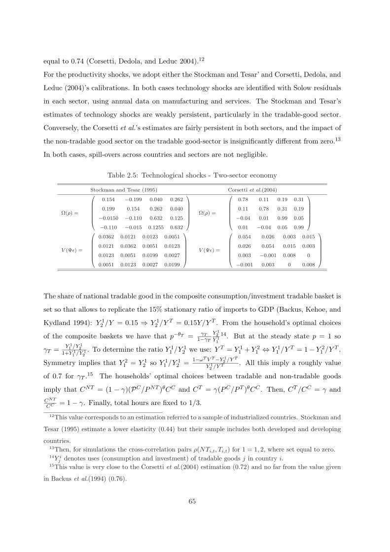
equal to 0.74 (Corsetti, Dedola, and Leduc 2004).12
For the productivity shocks, we adopt either the Stockman and Tesar’ and Corsetti, Dedola, and
Leduc (2004)’s calibrations. In both cases technology shocks are identified with Solow residuals
in each sector, using annual data on manufacturing and services. The Stockman and Tesar’s
estimates of technology shocks are weakly persistent, particularly in the tradable-good sector.
Conversely, the Corsetti et al.’s estimates are fairly persistent in both sectors, and the impact of
the non-tradable good sector on the tradable good-sector is insignificantly different from zero.13
In both cases, spill-overs across countries and sectors are not negligible.
Table 2.5: Technological shocks - Two-sector economy
Stockman and Tesar (1995) Corsetti et al.(2004)
Ω(ρ) =
0.154 −0.199 0.040 0.262
0.199 0.154 0.262 0.040
−0.0150 −0.110 0.632 0.125
−0.110 −0.015 0.1255 0.632
Ω(ρ) =
0.78 0.11 0.19 0.31
0.11 0.78 0.31 0.19
−0.04 0.01 0.99 0.05
0.01 −0.04 0.05 0.99
V (Ψε) =
0.0362 0.0121 0.0123 0.0051
0.0121 0.0362 0.0051 0.0123
0.0123 0.0051 0.0199 0.0027
0.0051 0.0123 0.0027 0.0199
V (Ψε) =
0.054 0.026 0.003 0.015
0.026 0.054 0.015 0.003
0.003 −0.001 0.008 0
−0.001 0.003 0 0.008
The share of national tradable good in the composite consumption/investment tradable basket is
set so that allows to replicate the 15% stationary ratio of imports to GDP (Backus, Kehoe, and
Kydland 1994): Y 12 /Y = 0.15 ⇒ Y 1
2 /Y T = 0.15Y/Y T . From the household’s optimal choices
of the composite baskets we have that p−θT = γT1−γT
Y 12
Y 11
14. But at the steady state p = 1 so
γT = Y 11 /Y 1
2
1+Y 11 /Y 1
2. To determine the ratio Y 1
1 /Y 12 we use: Y T = Y 1
1 + Y 21 ⇔ Y 1
1 /Y T = 1− Y 21 /Y T .
Symmetry implies that Y 21 = Y 1
2 so Y 11 /Y 1
2 = 1−ωT V T−Y 12 /Y T
Y 12 /Y T . All this imply a roughly value
of 0.7 for γT .15 The households’ optimal choices between tradable and non-tradable goods
imply that CNT = (1 − γ)(PC/PNT )θCC and CT = γ(PC/P T )θCC . Then, CT /CC = γ andCNT
CC = 1− γ. Finally, total hours are fixed to 1/3.
12This value corresponds to an estimation referred to a sample of industrialized countries. Stockman and
Tesar (1995) estimate a lower elasticity (0.44) but their sample includes both developed and developing
countries.13Then, for simulations the cross-correlation pairs ρ(NTi,t, Ti,t) for 1 = 1, 2, where set equal to zero.14Y i
j denotes uses (consumption and investment) of tradable goods j in country i.15This value is very close to the Corsetti et al.(2004) estimation (0.72) and no far from the value given
in Backus et al.(1994) (0.76).
65
Models evaluation
First of all, we note the general poor performance of this economy in almost all dimensions.
In particular regarding the US standard deviation of real per-capita output. Whereas with the
Stockman and Tesar’s (thereafter, ST ) calibration it is understated, with the Corsetti et al.’s
(thereafter, CDL) calibration it is largely overstated.
Regarding the international fluctuations, the striking implication from the ST calibration, where
shocks are weakly persistent, is the large dissociation of consumptions, for whatever specification
of preferences. However, even with weak persistent shocks (i.e. the TS calibration) the model
is able to reproduce positive cross-country correlations of investments and labor inputs. This
is at odds with the implications from the Stockman and Tesar (1995)’s pioneer model. The
key difference between our model and theirs is the structure of investment to each sector. In
the Stockman and Tesar’s model, each good is used for consumption and investment in its own
sector, so that capital is industry-specific. Conversely, we assume important linkages of goods on
both the demand side and the supply side. This explains why the quasi-perfect synchronization
of national and foreign economies under the CDL calibration, with larger persistence of shocks.
Finally, the intuitions we can drawn from the IRF functions (in particular in the CDL case) are
roughly the same as those from the two-goods economy. That is, the basic mechanisms of the
walrasian economy still at work following a positive shock to productivity in some sector. Look,
for instance, at figures 2.7 and 2.8, for the CDL calibration. The main differences with respect
to the IRF from national specialization economy are the hump-shaped response of country 2
variables and the instantaneous response of consumptions. The first one is due to either the
international diffusion of the shock and the international linkages of productions. On the other
hand, the dynamics of consumption are much harder to understand, mainly because their profile
is pretty the same for the two specifications of preferences.
The analogous IRF functions from the ST calibration are shown in figures B.1 and B.2 (see
appendix B.2). With respect to the IRF from the CDL calibration we remark that, because
shocks are less persistent, all variables come back to their steady state values in a few periods.
This is particularly true for the responses to a positive shock to the non-tradable-goods sector.
66
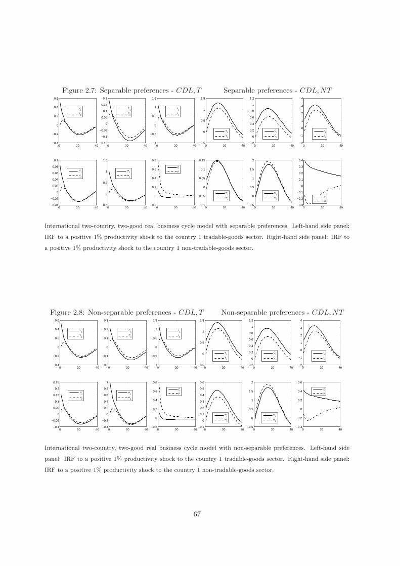
Figure 2.7: Separable preferences - CDL, T Separable preferences - CDL,NT
0 20 40−0.4
−0.2
0
0.2
0.4
0.6
Y1
Y2
0 20 40−0.15
−0.1
−0.05
0
0.05
0.1
0.15
0.2
C1
C2
0 20 40−1
−0.5
0
0.5
1
1.5
I1
I2
0 20 40−0.04
−0.02
0
0.02
0.04
0.06
0.08
0.1
H1
H2
0 20 40−0.5
0
0.5
1
1.5
w1
w2
0 20 40−0.2
0
0.2
0.4
0.6
0.8
E
p
0 20 40−0.5
0
0.5
1
1.5
Y1
Y2
0 20 40−0.2
0
0.2
0.4
0.6
0.8
1
1.2
C1
C2
0 20 40−2
−1
0
1
2
3
4
I1
I2
0 20 40−0.1
−0.05
0
0.05
0.1
0.15
H1
H2
0 20 40−0.5
0
0.5
1
1.5
2
w1
w2
0 20 40−0.3
−0.2
−0.1
0
0.1
0.2
0.3
0.4
E
p
International two-country, two-good real business cycle model with separable preferences. Left-hand side panel:
IRF to a positive 1% productivity shock to the country 1 tradable-goods sector. Right-hand side panel: IRF to
a positive 1% productivity shock to the country 1 non-tradable-goods sector.
Figure 2.8: Non-separable preferences - CDL, T Non-separable preferences - CDL, NT
0 20 40−0.4
−0.2
0
0.2
0.4
0.6
Y1
Y2
0 20 40−0.2
−0.1
0
0.1
0.2
0.3
C1
C2
0 20 40−1
−0.5
0
0.5
1
1.5
I1
I2
0 20 40−0.1
−0.05
0
0.05
0.1
0.15
0.2
0.25
H1
H2
0 20 40−0.4
−0.2
0
0.2
0.4
0.6
0.8
1
w1
w2
0 20 40−0.2
0
0.2
0.4
0.6
0.8
E
p
0 20 40−0.5
0
0.5
1
1.5
Y1
Y2
0 20 40−0.2
0
0.2
0.4
0.6
0.8
1
1.2
C1
C2
0 20 40−2
−1
0
1
2
3
4
I1
I2
0 20 40−0.1
0
0.1
0.2
0.3
0.4
0.5
0.6
H1
H2
0 20 40−0.5
0
0.5
1
1.5
2
w1
w2
0 20 40−0.4
−0.2
0
0.2
0.4
0.6
E
p
International two-country, two-good real business cycle model with non-separable preferences. Left-hand side
panel: IRF to a positive 1% productivity shock to the country 1 tradable-goods sector. Right-hand side panel:
IRF to a positive 1% productivity shock to the country 1 non-tradable-goods sector.
67
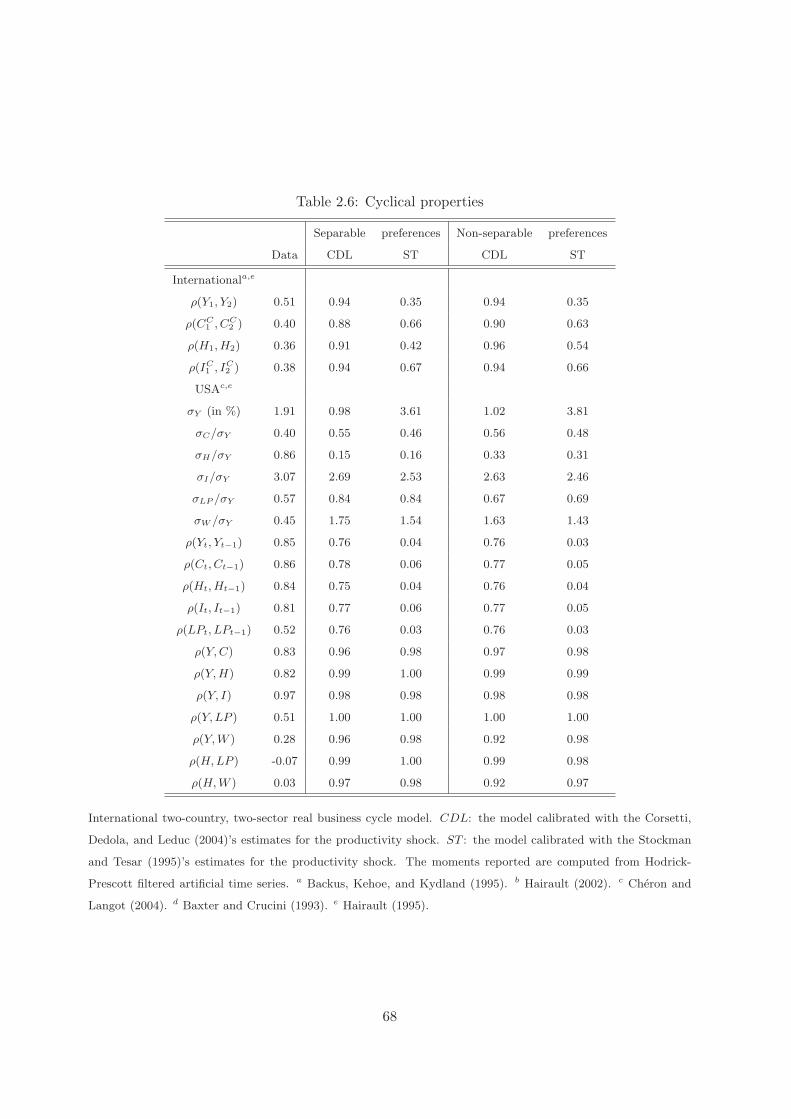
Table 2.6: Cyclical properties
Separable preferences Non-separable preferences
Data CDL ST CDL ST
Internationala,e
ρ(Y1, Y2) 0.51 0.94 0.35 0.94 0.35
ρ(CC1 , CC
2 ) 0.40 0.88 0.66 0.90 0.63
ρ(H1, H2) 0.36 0.91 0.42 0.96 0.54
ρ(IC1 , IC
2 ) 0.38 0.94 0.67 0.94 0.66
USAc,e
σY (in %) 1.91 0.98 3.61 1.02 3.81
σC/σY 0.40 0.55 0.46 0.56 0.48
σH/σY 0.86 0.15 0.16 0.33 0.31
σI/σY 3.07 2.69 2.53 2.63 2.46
σLP /σY 0.57 0.84 0.84 0.67 0.69
σW /σY 0.45 1.75 1.54 1.63 1.43
ρ(Yt, Yt−1) 0.85 0.76 0.04 0.76 0.03
ρ(Ct, Ct−1) 0.86 0.78 0.06 0.77 0.05
ρ(Ht, Ht−1) 0.84 0.75 0.04 0.76 0.04
ρ(It, It−1) 0.81 0.77 0.06 0.77 0.05
ρ(LPt, LPt−1) 0.52 0.76 0.03 0.76 0.03
ρ(Y, C) 0.83 0.96 0.98 0.97 0.98
ρ(Y, H) 0.82 0.99 1.00 0.99 0.99
ρ(Y, I) 0.97 0.98 0.98 0.98 0.98
ρ(Y, LP ) 0.51 1.00 1.00 1.00 1.00
ρ(Y, W ) 0.28 0.96 0.98 0.92 0.98
ρ(H, LP ) -0.07 0.99 1.00 0.99 0.98
ρ(H, W ) 0.03 0.97 0.98 0.92 0.97
International two-country, two-sector real business cycle model. CDL: the model calibrated with the Corsetti,
Dedola, and Leduc (2004)’s estimates for the productivity shock. ST : the model calibrated with the Stockman
and Tesar (1995)’s estimates for the productivity shock. The moments reported are computed from Hodrick-
Prescott filtered artificial time series. a Backus, Kehoe, and Kydland (1995). b Hairault (2002). c Cheron and
Langot (2004). d Baxter and Crucini (1993). e Hairault (1995).
68
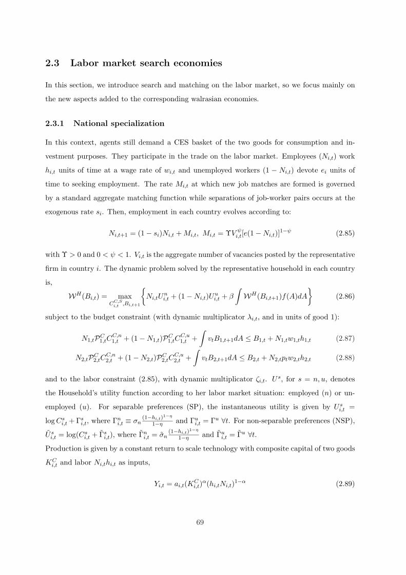
2.3 Labor market search economies
In this section, we introduce search and matching on the labor market, so we focus mainly on
the new aspects added to the corresponding walrasian economies.
2.3.1 National specialization
In this context, agents still demand a CES basket of the two goods for consumption and in-
vestment purposes. They participate in the trade on the labor market. Employees (Ni,t) work
hi,t units of time at a wage rate of wi,t and unemployed workers (1 − Ni,t) devote ei units of
time to seeking employment. The rate Mi,t at which new job matches are formed is governed
by a standard aggregate matching function while separations of job-worker pairs occurs at the
exogenous rate si. Then, employment in each country evolves according to:
Ni,t+1 = (1− si)Ni,t + Mi,t, Mi,t = ΥV ψi,t[e(1−Ni,t)]1−ψ (2.85)
with Υ > 0 and 0 < ψ < 1. Vi,t is the aggregate number of vacancies posted by the representative
firm in country i. The dynamic problem solved by the representative household in each country
is,
WH(Bi,t) = maxCC,S
i,t ,Bi,t+1
Ni,tU
ni,t + (1−Ni,t)Uu
i,t + β
∫WH(Bi,t+1)f(A)dA
(2.86)
subject to the budget constraint (with dynamic multiplicator λi,t, and in units of good 1):
N1,tPC1,tC
C,n1,t + (1−N1,t)PC
1,tCC,u1,t +
∫vtB1,t+1dA ≤ B1,t + N1,tw1,th1,t (2.87)
N2,tPC2,tC
C,n2,t + (1−N2,t)PC
2,tCC,u2,t +
∫vtB2,t+1dA ≤ B2,t + N2,tptw2,th2,t (2.88)
and to the labor constraint (2.85), with dynamic multiplicator ζi,t. U s, for s = n, u, denotes
the Household’s utility function according to her labor market situation: employed (n) or un-
employed (u). For separable preferences (SP), the instantaneous utility is given by U si,t =
log Csi,t + Γs
i,t, where Γni,t ≡ σn
(1−hi,t)1−η
1−η and Γui,t = Γu ∀t. For non-separable preferences (NSP),
U si,t = log(Cs
i,t + Γsi,t), where Γn
i,t = σn(1−hi,t)
1−η
1−η and Γui,t = Γu ∀t.
Production is given by a constant return to scale technology with composite capital of two goods
KCi,t and labor Ni,thi,t as inputs,
Yi,t = ai,t(KCi,t)
α(hi,tNi,t)1−α (2.89)
69
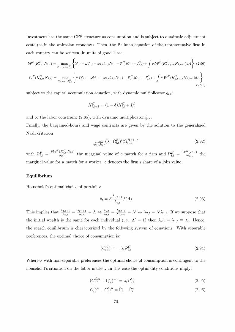
Investment has the same CES structure as consumption and is subject to quadratic adjustment
costs (as in the walrasian economy). Then, the Bellman equation of the representative firm in
each country can be written, in units of good 1 as:
WF (KC1,t, N1,t) = max
N1,t+1,IC1,t
Y1,t−ωV1,t−w1,th1,tN1,t−PC
1,t(C1,t + IC1,t)+
∫vtWF (KC
1,t+1, N1,t+1)dA
(2.90)
WF (KC2,t, N2,t) = max
N2,t+1,IC2,t
pt(Y2,t − ωV2,t − w2,th2,tN2,t)− PC
2,t(C2,t + IC2,t) +
∫vtW
F (KC2,t+1, N2,t+1)dA
(2.91)
subject to the capital accumulation equation, with dynamic multiplicator qi,t:
KCi,t+1 = (1− δ)KC
i,t + ICi,t
and to the labor constraint (2.85), with dynamic multiplicator ξi,t.
Finally, the bargained-hours and wage contracts are given by the solution to the generalized
Nash criterion
maxwi,t,hi,t
(λi,tΩFi,t)
ε(ΩHi,t)
1−ε (2.92)
with ΩFi,t =
∂WF (KCi,t,Ni,t)
∂Ni,tthe marginal value of a match for a firm and ΩH
i,t = WH(Bi,t)∂Ni,t
the
marginal value for a match for a worker. ε denotes the firm’s share of a jobs value.
Equilibrium
Household’s optimal choice of portfolio:
vt = βλi,t+1
λi,tf(A) (2.93)
This implies that λ1,t+1
λ1,t= λ2,t+1
λ2,t= Λ ⇔ λ2,t
λ1,t= λ2,t+1
λ1,t+1= Λ′ ⇔ λ2,t = Λ′λ1,t. If we suppose that
the initial wealth is the same for each individual (i.e. Λ′ = 1) then λ2,t = λ1,t ≡ λt. Hence,
the search equilibrium is characterized by the following system of equations. With separable
preferences, the optimal choice of consumption is:
(CCi,t)
−1 = λtPCi,t (2.94)
Whereas with non-separable preferences the optimal choice of consumption is contingent to the
household’s situation on the labor market. In this case the optimality conditions imply:
(CC,ui,t + Γu
i,t)−1 = λtPC
i,t (2.95)
CC,ni,t − CC,u
i,t = Γui − Γn
i (2.96)
70
Moreover, the aggregate consumption in each country must satisfy:
CCi,t = Ni,tC
C,ni,t + (1−Ni,t)C
C,ui,t (2.97)
On the other hand, with separable preferences the hours contracts are:
(1− α)Y1,t
N1,th1,t=
σn
λt(1− h1,t)−η (2.98)
(1− α)Y2,t
N2,th2,t=
σn
ptλt(1− h2,t)−η (2.99)
and the wage contracts are:
(1− ε)
(1− α)Y1,t
N1,t+
ωV1,t
1−N1,t
+ ε
[Γu1 − Γn
1,t]λt
= w1,th1,t (2.100)
(1− ε)
(1− α)Y2,t
N2,t+
ωV2,t
1−N2,t
+ ε
[Γu2 − Γn
2,t]ptλt
= w2,th2,t (2.101)
Whereas with non-separable preferences we have:
(1− α)Y1,t
N1,th1,t= PC
1,tσn(1− h1,t)−η (2.102)
(1− α)Y2,t
N2,th2,t=PC
2,tσn
pt(1− h2,t)−η (2.103)
and,
(1− ε)
(1− α)Y1,t
N1,t+ ω
V1,t
1−N1,t
+ εPC
1,t[Γu − Γn
1,t] = w1,th1,t (2.104)
(1− ε)
(1− α)Y2,t
N2,t+ ω
V2,t
1−N2,t
+ ε
PC2,t[Γ
u − Γn2,t]
pt= w2,th2,t (2.105)
Then, the worker’s wage bill (equations (3.17), (3.19) and (2.104), (2.105)) is a weighted average
of (i) her contribution to output plus the hiring costs per unemployed worker, and (ii) her
outside opportunities. Remark that with separable preferences the outside opportunities are
affected by income and intertemporal substitution effects, through variations in λt.
The intertemporal allocation of consumption and leisure is such that the marginal contribution
of one hour of labor for the firm is equal to the marginal cost of one worked hour for the
household. As the wage bill, the allocation of time is affected by income and intertemporal
substitution effects in the case of separable preferences.
Let us think to the impact of an economic boom relying on a positive temporary, orthogonal
technological shock to country i. With separable preferences, the productivity shock leads to a
higher labor productivity and hiring costs, whereas the decrease in λt which arises at economic
71
boom increases the outside options. That is, the dynamics of the real wage in this context
is a combination of two procyclical components. Conversely, as the non-separable preferences
have the property that, from an ex post perspective, employed agents are actually better off
than unemployed agents, and can take more advantage of an economic boom. This depresses
the outside options, in putting a downward pressure on the real wage (see Cheron and Langot
(2004) for a deeper discussion in a closed-economy context).
The firm’s optimal choices of employment and capital are respectively:
ξ1,t ≡ ωV1,t
M1,t(2.106)
ξ2,t ≡ ptωV2,t
M2,t(2.107)
ξ1,t = βEt
[λt+1
λt
((1− α)
Y1,t+1
N1,t+1− w1,t+1h1,t+1 + (1− s)ξ1,t+1
)](2.108)
ξ2,t = βEt
[λt+1
λt
(pt+1(1− α)
Y2,t+1
N2,t+1− pt+1w2,t+1h2,t+1 + (1− s)ξ2,t+1
)](2.109)
qi,t = PCi,t(1 + φ(IC
i,t − δKCi,t)) (2.110)
q1,t = βEt
[λt+1
λt
(α
Y1,t+1
KC1,t+1
+ q1,t+1 − δPC1,t+1
)](2.111)
q2,t = βEt
[λt+1
λt
(α
ptY2,t+1
KC2,t+1
+ q2,t+1 − δPC2,t+1
)](2.112)
The labor decision (equations (2.106)-(2.109)) are very similar to the capital ones (equations
(2.110)-(2.112)). That is, firms view their existing workforce as a capital asset because finding
new workers takes time and effort. Together mean that the number of vacancies posted by
each firm is such that the average cost of creating a job at date t, ξi,t, is equal to the expected
discounted marginal value of one job at date t+1: the marginal productivity net of the marginal
cost of labor plus the average cost of creating a job at t + 1.
In this setting, the equilibrium in the goods market is given by:
Y1,t = C11,t + C2
1,t + I11,t + I2
1,t + C1,t + ω1V1,t (2.113)
Y2,t = C12,t + C2
2,t + I12,t + I2
2,t + C2,t + ω2V2,t (2.114)
72
2.3.2 The single good economy
Both countries produce the same final good. Since there is a single good, international trade
takes place only to smooth consumption and to ensure that capital is allocated in the most
productive country. In the variant of the model with restricted asset markets agents only can
trade goods and non-contingent real debt, as was done in the walrasian economy. Finally, since
the consumption/investment good is internationally mobile, there is a single resource constraint
for this good:
Y1,t + Y2,t = C1,t + C2,t + I1,t + I2,t + C1,t + C2,t (2.115)
2.3.3 Empirical results
Calibration. We briefly describe the calibration of the parameters and values specific to the
search economies. The detailed procedure and main sources are given in next chapter. Aggregate
expenditures on search activity are set in each sector equal to 1 % of output: ωV/Y = 0.01. The
quarterly rate of transition from employment to nonemployment is set equal to N = 0.6. η is
fixed at 5, a fairly standard value. To guaranty that the equilibrium unemployment is socially-
efficient we set both, the elasticity of the matching function with respect to vacancies and the
firms’ bargaining power, at ε = ψ = 0.6. We fix h = 1/3 and the average fraction of time that
unemployed households devote to search equal to e = h/2. The rate at which vacancies become
productive is m = 0.9. The remaining values of endogenous variables are computed from the
equilibrium equations evaluated at the steady state.
Table 2.7 reports statistics concerning the international fluctuations of industrialized countries
and the US real wage dynamics. These results correspond to average values from actual and
theoretical series filtered with the Hodrick-Prescott filter. Models include the one-good labor
market search economy (LMS1) and the Hairault’s type two-good labor market search economy
(LMS2). Simulations results are completed by Impulse Response Functions (IRF).
We first concentrate on the effects of two hypotheses: the non-separability of consumption and
leisure in the utility function, and the search in the labor market (LMS1). From table 2.7 we
point out that (see also the IRF showed in figure 2.9 and figure 2.10): the positive cross-country
correlations of outputs and labor inputs, as well as the dissociation of national and foreign
consumptions seem mostly explained by the non-separability hypothesis. On the other hand,
the search hypothesis accounts for the positive correlation of investments and the additional
73
Table 2.7: Cyclical properties - Search economies
Data LMS1 LMS1 LMS1-IM LMS2 LMS2
SP NSP NSP SP NSP
Internationala,e
ρ(Y1, Y2) 0.51 -0.03 0.48 0.50 0.29 0.57
ρ(CC1 , CC
2 ) 0.40 1.00 0.58 0.54 0.69 0.49
ρ(H1, H2) 0.36 -0.88 0.64 0.66 0.05 0.77
ρ(IC1 , IC
2 ) 0.38 0.64 0.95 0.95 0.35 0.86
στ/σY 1.90 – – – 0.76 0.43
σΓ/σY 3.28 – – – 0.53 0.30
USAc,e
σY (in %) 1.91 1.42 1.98 2.00 1.22 2.03
σC/σY 0.40 0.54 0.66 0.69 0.68 0.70
σH/σY 0.86 0.52 0.85 0.85 0.21 0.85
σI/σY 3.07 1.26 2.34 2.37 1.61 2.46
σLP /σY 0.57 0.68 0.40 0.39 0.83 0.40
σW /σY 0.45 0.59 0.22 0.21 0.78 0.23
ρ(Yt, Yt−1) 0.85 0.77 0.85 0.85 0.72 0.86
ρ(Ct, Ct−1) 0.86 0.74 0.85 0.87 0.73 0.85
ρ(Ht, Ht−1) 0.84 0.89 0.91 0.91 0.89 0.91
ρ(It, It−1) 0.81 0.74 0.71 0.72 0.73 0.74
ρ(LPt, LPt−1) 0.52 0.62 0.43 0.46 0.64 0.48
ρ(Y, C) 0.83 0.70 0.75 0.80 0.97 0.77
ρ(Y, H) 0.82 0.78 0.92 0.92 0.85 0.92
ρ(Y, I) 0.97 0.92 0.84 0.84 1.00 0.88
ρ(Y, LP ) 0.51 0.88 0.54 0.54 0.99 0.55
ρ(Y, W ) 0.28 0.83 0.60 0.60 0.99 0.62
ρ(Y, LS) -0.30 -0.60 -0.47 -0.46 -0.59 -0.43
ρ(H, LP ) -0.07 0.38 0.17 0.16 0.77 0.18
ρ(H, W ) 0.03 0.34 0.24 0.23 0.81 0.27
The moments reported are computed from Hodrick-Prescott filtered artificial time series. a Backus, Kehoe, and
Kydland (1995). b Hairault (2002). c Cheron and Langot (2004). d Baxter and Crucini (1993). e Hairault (1995).
74
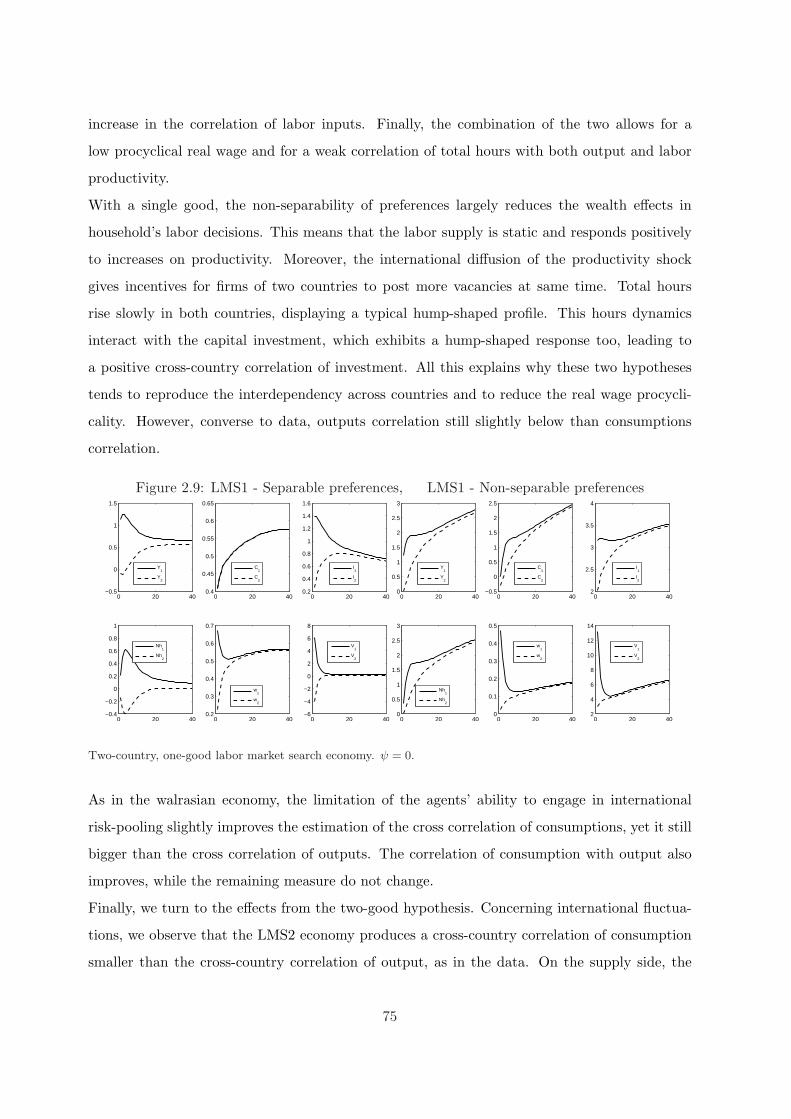
increase in the correlation of labor inputs. Finally, the combination of the two allows for a
low procyclical real wage and for a weak correlation of total hours with both output and labor
productivity.
With a single good, the non-separability of preferences largely reduces the wealth effects in
household’s labor decisions. This means that the labor supply is static and responds positively
to increases on productivity. Moreover, the international diffusion of the productivity shock
gives incentives for firms of two countries to post more vacancies at same time. Total hours
rise slowly in both countries, displaying a typical hump-shaped profile. This hours dynamics
interact with the capital investment, which exhibits a hump-shaped response too, leading to
a positive cross-country correlation of investment. All this explains why these two hypotheses
tends to reproduce the interdependency across countries and to reduce the real wage procycli-
cality. However, converse to data, outputs correlation still slightly below than consumptions
correlation.
Figure 2.9: LMS1 - Separable preferences, LMS1 - Non-separable preferences
0 20 40−0.5
0
0.5
1
1.5
Y1
Y2
0 20 400.4
0.45
0.5
0.55
0.6
0.65
C1
C2
0 20 400.2
0.4
0.6
0.8
1
1.2
1.4
1.6
I1
I2
0 20 40−0.4
−0.2
0
0.2
0.4
0.6
0.8
1
Nh1
Nh2
0 20 400.2
0.3
0.4
0.5
0.6
0.7
w1
w2
0 20 40−6
−4
−2
0
2
4
6
8
V1
V2
0 20 400
0.5
1
1.5
2
2.5
3
Y1
Y2
0 20 40−0.5
0
0.5
1
1.5
2
2.5
C1
C2
0 20 402
2.5
3
3.5
4
I1
I2
0 20 400
0.5
1
1.5
2
2.5
3
Nh1
Nh2
0 20 400
0.1
0.2
0.3
0.4
0.5
w1
w2
0 20 402
4
6
8
10
12
14
V1
V2
Two-country, one-good labor market search economy. ψ = 0.
As in the walrasian economy, the limitation of the agents’ ability to engage in international
risk-pooling slightly improves the estimation of the cross correlation of consumptions, yet it still
bigger than the cross correlation of outputs. The correlation of consumption with output also
improves, while the remaining measure do not change.
Finally, we turn to the effects from the two-good hypothesis. Concerning international fluctua-
tions, we observe that the LMS2 economy produces a cross-country correlation of consumption
smaller than the cross-country correlation of output, as in the data. On the supply side, the
75
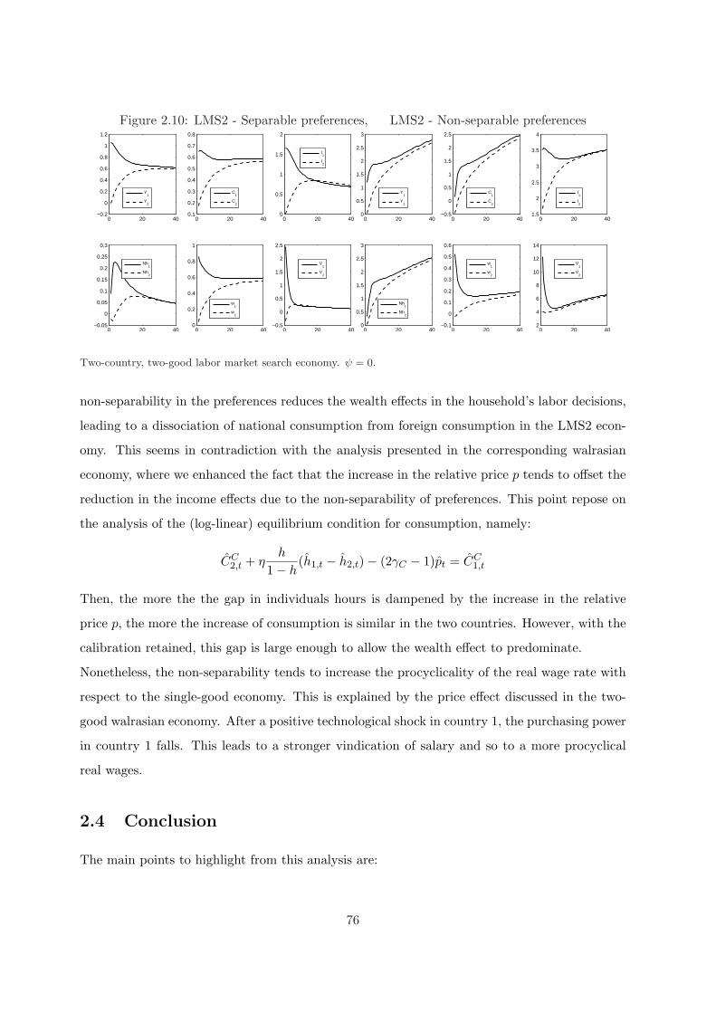
Figure 2.10: LMS2 - Separable preferences, LMS2 - Non-separable preferences
0 20 40−0.2
0
0.2
0.4
0.6
0.8
1
1.2
Y1
Y2
0 20 400.1
0.2
0.3
0.4
0.5
0.6
0.7
0.8
C1
C2
0 20 400
0.5
1
1.5
2
I1
I2
0 20 40−0.05
0
0.05
0.1
0.15
0.2
0.25
0.3
Nh1
Nh2
0 20 400
0.2
0.4
0.6
0.8
1
w1
w2
0 20 40−0.5
0
0.5
1
1.5
2
2.5
V1
V2
0 20 400
0.5
1
1.5
2
2.5
3
Y1
Y2
0 20 40−0.5
0
0.5
1
1.5
2
2.5
C1
C2
0 20 401.5
2
2.5
3
3.5
4
I1
I2
0 20 400
0.5
1
1.5
2
2.5
3
Nh1
Nh2
0 20 40−0.1
0
0.1
0.2
0.3
0.4
0.5
0.6
w1
w2
0 20 402
4
6
8
10
12
14
V1
V2
Two-country, two-good labor market search economy. ψ = 0.
non-separability in the preferences reduces the wealth effects in the household’s labor decisions,
leading to a dissociation of national consumption from foreign consumption in the LMS2 econ-
omy. This seems in contradiction with the analysis presented in the corresponding walrasian
economy, where we enhanced the fact that the increase in the relative price p tends to offset the
reduction in the income effects due to the non-separability of preferences. This point repose on
the analysis of the (log-linear) equilibrium condition for consumption, namely:
CC2,t + η
h
1− h(h1,t − h2,t)− (2γC − 1)pt = CC
1,t
Then, the more the the gap in individuals hours is dampened by the increase in the relative
price p, the more the increase of consumption is similar in the two countries. However, with the
calibration retained, this gap is large enough to allow the wealth effect to predominate.
Nonetheless, the non-separability tends to increase the procyclicality of the real wage rate with
respect to the single-good economy. This is explained by the price effect discussed in the two-
good walrasian economy. After a positive technological shock in country 1, the purchasing power
in country 1 falls. This leads to a stronger vindication of salary and so to a more procyclical
real wages.
2.4 Conclusion
The main points to highlight from this analysis are:
76

• The international comovement of the macro aggregates is well reproduced by the stan-
dard walrasian model once international linkages between the outputs are added via the
introduction of more than one good.
• However, in the two-good economy the variations in the relative price of goods offset the
reduction in the wealth effect allowed by the non-separability of preferences, which in turn
may lead to worst predictions for the cross-country correlation of consumption than with
standard additively separable preferences.
• Even if the restricted asset markets structure plays a role in mitigating with the comove-
ment puzzle, it is not enough to replicate the observed international fluctuations.
• Regarding the search economies, we show that in the single-god economy, the combination
of search and matching in the labor market with the non-separability is enough to predict
positive comovements of labor inputs and investments as well as a large dissociation of
consumptions. Moreover, the procyclicality of real wage rate is reduced, and the correlation
of total hours with both output and labor productivity is low. Then, the three puzzles are
partially solved.
• Finally we show that the gain from including two goods in that framework is that the
model is able now to replicate a correlation of outputs bigger than that of consumptions
(Hairault 2002). However, the price dynamics provoked by a positive productivity shock
decrease the agent’s purchasing power, leading to a stronger vindication of salary and so
to a slightly more procyclical real wages.
77

Chapter 3
Tax/Benefit system and labor
market search: reconciling the
standard separable preferences with
the real wage dynamics and the
international business cycles
This chapter is built on the basis of a joint working paper with Francois Langot
78
Introduction
Traditional real business cycle models assume that technological change is the driving force be-
hind growth and fluctuations observed in developed economies, in particular the U.S.. While
these models have been successful in accounting for a large fraction of the variability and co-
movements of the aggregate time series, they do not do well along some dimensions1 As is well
known, relative to the data, the variability of consumption, hours of work, and output is too
low, and the variability of investment is too high. But maybe the main failure is the predicted
correlation of real wages with both hours worked and output. In such a models, variations in
technology shifts the labor demand curve but not the labor supply curve, thus inducing a strong
positive correlation between wages and hours. The introduction of search and matching in the
labor market (Andolfatto 1996) outperforms the model predictions along these lines2.
This line of reasoning naturally suggests that to improve the predictions from the real business
cycle models one must include something that shifts labor supply. If both labor demand and
labor supply shift, then the strong positive correlation between hours and wages can probably
be reduced.
Several candidate labor supply shifters have already been considered, such as home production
(Benhabib, Rogerson, and Wright 1991) or government consumption (Christiano and Eichen-
baum 1992). As it is shown by Burnside, Eichenbaum, and Fisher (2004), we also observe large
changes in the tax rates. In the Keynesian tradition, fiscal policy, and therefore taxation, is
one of the main instruments to stabilize the economy. However, in the 1990s, several pioneering
works considered taxation as a source of business cycle fluctuations. This feeds the criticisms
about the possibility to use taxes as stabilization tool.
As Christiano and Eichenbaum (1992) show, the inclusion of a public sector has the potential to
improve some of the predictions of the standard real business cycle model. In particular, they
study a real business cycle model in which government purchases affect the agents’ utility. The
expenditures are financed through lump-sum taxes. In this case, shocks to expenditures shift
the labor supply curve. However, they predict that while the hours and wage correlation comes
closer to that observed, it is significantly positive. But Christiano and Eichenbaum (1992) do not
allow for distortionary taxation. Intuitively, like government expenditures, shocks to income and
payroll taxes can be interpreted as shocks to labor supply, as opposed to technology shocks which1See chapter 1 and chapter 2 of this thesis.2See chapter 2.
79
may be interpreted as shocks to labor demand. Thus, tax rates provide another mechanism for
explaining the observed correlation between hours and wages.
In this line of research, some pioneering articles have shown that stochastic fiscal policy improves
the performance of real business cycle models. McGrattan (1994) finds that a significant portion
of the variance of the aggregate consumption, output, hours worked, capital stock, and invest-
ment can be attributed to the factor tax (i.e. on capital and labor income) and government
spending processes. Similarly, Braun (1994) shows that modelling fluctuations in personal and
corporate income tax rates increases the model’s predicted relative variability of hours and de-
creases its predicted correlation between hours and average productivity. Finally, using Swedish
data, ?) find that the empirical fit of a simple stochastic growth model is significantly improved
when it is amended to include imperfectly predictable fluctuations in payroll taxes, consumption
taxes and government consumption.3
In all cases, the basic mechanisms at work are as follows. Taxes to labor alter the leisure/labor
supply decision, highlighting the volatility of hours worked. In plain words, if income and payroll
taxes fluctuate over time, it is optimal to work hard when taxes are relatively low and to take time
off when they are relatively high. Then, as labor taxes fluctuate, so do hours worked. Similarly,
a temporarily high tax rate on consumption provides an incentive to postpone consumption to
a later date, when the tax rate is likely to be lower. Hence, as the consumption tax fluctuates,
so does consumption. Consequently, the inclusion of such a taxes should increase the predicted
volatility of hours and consumption, bringing the implications of theory closer to the facts.
Finally, the variability in investment and capital increases either because of increases in the
capital tax, or indirectly by the complementarity of capital and labor, and even though the
agents’ trade-off between consumption and saving following a consumption tax shock.
In quantitative terms, these models yield to predictions for the correlation between hours and
real wages, as measured by average productivity, close to the empirical correlation. Likewise,
the predicted variability of hours worked and consumption are much closer to their empirical
values when fiscal policy is included (even if in general the relative volatility of aggregate hours
is overstated). Nevertheless, these former papers show two drawbacks. The first one is that all of
them consider a closed economy, so that the possible variability in the macro aggregates passing
through the international trade is not accounted for. The second one is that the theoretical3Moreover, they find that for large sets of conventional moments, models with stochastic fiscal policy cannot
be statistically rejected, whereas a model without it is always rejected.
80

real wage is measured by average productivity. This obviously prevents from analyzing other
features of the US labor market, such as the lower volatility of the real wage than the one of the
labor productivity.
Then, in this chapter we show that fluctuations in distortive taxes can account for some of
the puzzling features of the U.S. business cycle. Namely, the observed real wage rigidity, the
international comovement of investment and labor inputs, and the so-called consumption corre-
lation puzzle (according to which cross-country correlations of output are higher than the one
of consumption). This is done in a two-country search and matching model with fairly standard
preferences, extended to include a tax/benefit system. In this simple framework, the tax side is
represented by taxation on labor income, employment (payroll tax) and consumption, whereas
the benefit side is resumed by the unemployment benefits and the worker’s bargaining power.
The main departures from the former literature on taxation as a source of business cycle fluctu-
ations are twofold. First, we consider a two-country general equilibrium model, so that we are
able to discuss the effects on the observed international fluctuations. Second, we assume search
and matching in the labor market. Our model is close to the Hairault (2002)’s one, who de-
velops a two-country, two-good search model, able to explain the puzzling facts of international
fluctuations once a non-separability in the agents’ preferences is considered4.
Our model is also close to the Cheron and Langot (2004)’s model, who explain the real wage
rigidity in a closed-economy search model by means of a particular set of non-separable prefer-
ences.
Either in the Hairault (2002)’s paper or in the Cheron and Langot (2004)’s paper, the non-
separability of preferences plays a main role. However, this hypothesis is unable to simultane-
ously account for the real wage rigidity and for the observed international fluctuations. Con-
versely, in this work we show that all those facts can be accounted in a single framework with
fairly standard preferences. On the one side, an economic boom accompanied of a positive shock
to the labor taxes leads to countercyclical outside options, which dampens the procyclicality of
the real wage. On the other side, under the national specialization hypothesis, the equalization
of consumptions across countries following a productivity shock does not hold anymore, (even
in presence of separable preferences), and the gap between domestic and foreign consumption
increases as long as the consumption tax is shocked too.4See chapter 2.
81
3.1 The Model
The world economy consists of two countries (country 1 or home country and country 2 or
foreign country), each represented by a large number of identical consumers and a production
technology. Population size is normalized to unity. Each country specializes in the production
of a single good. The main source of fluctuations are persistent shocks to productivity that
are internationally diffused. Additionally, both countries are affected by shocks to taxes on
consumption and labor (i.e. , taxes on labor income and payroll taxes). The countries are
linked either on the consumption and the production side since agents demand a CES basket
of the two goods for consumption and investment purposes. Finally, agents participate in the
trade on the labor market.
3.1.1 Labor market flows
Employment in country i = 1, 2 is predetermined at each time and changes only gradually as
workers separate from jobs, at the exogenous rate si, or unemployed agents find jobs, at the
hiring rate Mi,t. Let Ni,t and Vi,t, respectively be the number of workers and the total number
of new jobs made available by firms, then employment evolves according to
Ni,t+1 = (1− si)Ni,t + Mi,t, Mi,t = V φi,t[ei(1−Ni,t)]1−φ, 0 < φ < 1
where ei > 0 and 0 < si < 1 are the constant search effort and the exogenous separation rate of
job-worker pairs.
3.1.2 Households
At any period, Ni agents are employed while the remaining 1−Ni are unemployed. Unemployed
agents are randomly matched with job vacancies. Employees work hi units of time at a wage
rate of wi. Unemployed workers devote ei units of their time seeking employment and receive
the unemployment benefits bi. In both cases they pay a labor income tax levied at rate τ iw.
Markets are complete, so we can derive the intertemporal decision rules by solving the program
of a representative household. This agent consumes a CES basket of the two goods (Hairault
2002):
CC,zi =
[γ
1θ C
θ−1θ
i + (1− γ)1θ C
θ−1θ
j 6=i
] θθ−1
, for z = n, u, i = 1, 2
82
where CC,n and CC,u respectively stand for the consumption of employed and unemployed
agents. θ is the elasticity of substitution between the two goods and γ is the share of the
national good in the consumption basket. The price index of the composite goods is defined as:
PCi =
[γP 1−θ
i + (1− γ)P 1−θj 6=i
] 11−θ
, for i = 1, 2.
with Pi the production price of good i.
We still assume perfect international risk sharing: households in the two countries have access
to contingent claims Bi,t = Bi(At) at prices vt = v(At+1) providing one unit of good 1 if the
state A occurs at t+1. That is, we take the good produced in country 1 as accounting unit, and
we normalize its value to 1. The representative household in country i is assumed to maximize
the expected discounted sum of its utility flows,
WH(Bi,t) = maxCC,n
i,t ,CC,ui,t ,Bi,t
Ni,tU(CC,n
i,t , 1− hi,t) + (1−Ni,t)U(CC,ui,t , 1− ei) + β
∫WH(Bi,t+1)f(A)dAt+1
(3.1)
subject to the labor constraint:
Ni,t+1 = (1− s)Ni,t + Ψi,t(1−Ni,t), for i=1,2 (3.2)
where Ψi,t ≡ Mi,t/(1 − Ni,t) is the rate at which unemployed agents find jobs, and subject to
the budget constraint:
(1 + τ1c,t)
[N1,tPC
1,tCC,n1,t + (1−N1,t)PC
1,tCC,u1,t
]+
∫vtB1,t+1dAt+1 ≤ B1,t + (3.3)
(1− τ1w,t)[N1,tw1,th1,t + (1−N1,t)b1,t] + L1,t, for i=1
(1 + τ2c,t)
[N2,tPC
2,tCC,n2,t + (1−N2,t)PC
2,tCC,u2,t
]+
∫vtB2,t+1dAt+1 ≤ B2,t + (3.4)
(1− τ1w,t)pt[N2,tw2,th2,t + (1−N2,t)b2,t] + L2,t, for i=2
and given some initial conditions (Ni,0, Bi,0). pt ≡ P2,t
P1,t, PC
i,t ≡P C
i,t
P1,tand Li,t are lump-sum
transfers from the government to be defined below. f(A) ≡ f(At+1, At) denotes the density
function describing the transition from the state At to the state At+1. τ ic , τ i
w stand respectively
for the consumption tax rate and the labor income tax rate prevailing in country i.
The contemporaneous utility function is assumed to be increasing and concave in both arguments
and exhibits conventional additive separability between consumption (CC,zi,t ) and leisure (Lz
i,t):
Ui,t(CC,zi,t , Lz
i,t) = log CC,zi,t + Γz
i,t ≡ U zi,t, z = n, u (3.5)
83

where Γni,t ≡ σ
(1−hi,t)1−η
1−η with σ, η > 0 and Γui,t = Γu
i ∀t. The parameter σ can be interpreted as
reflecting differences in the efficiency of household’s home production technology across different
states of employment opportunities.
3.1.3 Firms
Each country specializes in the production of a single good. The representative firm in country
i = 1, 2 has a constant returns-to-scale technology that uses composite capital and labor hours
to produce output,
Yi,t = ai,tKαi,t(Ni,thi,t)1−α, 0 < α < 1 (3.6)
The primary source of fluctuations are persistent shocks to aggregate productivity, represented
by ai,t. The stochastic productivity vector at = [a1,t, a2,t]′ is assumed to follow a V AR(1) process
in natural logarithms:
ln at+1 = Ω ln at + ϑεt+1 , where εt+1 ∼ iid N (0, I)
The vector εt = [ε1, ε2]′ represents the innovations to productivity variables. The matrix Ω,
defined by
Ω =
ρ1,1 ρ1,2
ρ2,1 ρ2,2
describes the autoregressive component of the disturbance. Finally, the covariances between the
elements are given by the matrix ϑ, defined by
ϑ =
1 υ1,2
υ2,1 1
This matrix reflects the extent to which the shocks are idiosyncratic or global in nature.
New capital goods are internationally mobile. Investment has the same CES structure as con-
sumption (and then, the same price PiC) and is subject to quadratic adjustment costs:
Ci,t =φ
2(Ki,t+1 −Ki,t)2
Let ωi be the unitary cost of a vacancy job. Firms seek to maximize the discounted value of the
dividend flows,
WF (Ki,t, Ni,t) = maxVi,t,Ii,t
πi,t +
∫vtWF (Ki,t+1, Ni,t+1)dAt+1
for πi,t = Pi,t
(Yi,t − ωiVi,t − (1 + τ i
f,t)wi,tNi,thi,t − Ci,t
)− P ci,tI
ci,t (3.7)
84

subject to the constraints,
Ni,t+1 = (1− si)Ni,t + Φi,tVi,t (3.8)
Ki,t+1 = (1− δ)Ki,t + Ici,t (3.9)
and given some initial conditions (Ni,0,Ki,0), where 0 < δ < 1 is the depreciation rate of capital.
Φi,t ≡ Mi,t/Vi,t is the rate at which vacancies and workers are matched and τ if stands for the
country-specific payroll tax payed by firms.
3.1.4 Government
The government levies taxes to finance expenditures. We assume a balanced budget at each
period, so that any revenue that is not used to finance current purchases is transferred to
households in a lump-sum payment. Thus, real transfers to country i households are given by:
L1,t = τ1c,tPC
1,t[N1,tCC,n1,t +(1−N1,t)C
C,u1,t ]+(τ1
f,t +τ1w,t)w1,th1,tN1,t−b1,t(1−τ1
w,t)(1−N1,t) (3.10)
L2,t = τ2c,tPC
2,t[N2,tCC,n2,t + (1−N2,t)C
C,u2,t ] + pt(τ2
f,t + τ2w,t)w2,th2,tN2,t − b2,tpt(1− τ2
w,t)(1−N2,t)
(3.11)
In order to be coherent with our estimations (section 3.2), we assume that the stochastic process
governing tax rate τ ij , for j = c, w, f , follows an AR(1),
τ ij,t+1 = (1− ρi
j)τij + ρi
jτij,t + εi
j,t+1, with εij,t ∼ N (0, σi
j) (3.12)
with τ ij denoting the mean value of the tax variable τ i
j,t.
3.1.5 Nash bargaining
Wages and hours worked are derived from the generalized Nash-bargaining model (Pissarides
2000), with firm’s relative bargaining power εi:
maxwi,t,hi,t
(λtVFt )εi(VH
i,t)1−εi (3.13)
with VFi,t =
∂W(ΩFi,t)
∂Ni,tthe marginal value of a match for a firm and VH
i,t =W(ΩF
i,t)
∂Ni,tthe marginal
value for a match for a worker. Matter of simplicity, we define the labor tax: τni,t ≡
1+τ if,t
1−τ iw,t
.
It is worth stressing that, under the separability assumption, optimal households’ decision rules
imply
CC,ni,t = CC,u
i,t ≡ CCi,t (3.14)
Uui,t = Un
i,t +(Γu
i − Γni,t
)(3.15)
85

This entails the following hours worked contracts, for i = 1:(
1− τ1w,t
1 + τ1f,t
)(1− α)
Y1,t
N1,th1,t= σ
(1− h1,t)−η
λ1,t(3.16)
⇔(
1− τ1w,t
(1 + τ1f,t)(1 + τ1
c,t)
)(1− α)
Y1,t
N1,th1,t= σ(1− h1,t)−ηPC
i,tCCi,t
and the following wages contracts, for i = 1:
Labor cost
(1 + τ1f,t)w1,th1,t = (1− ε1)
[(1− α)
Y1,t
N1,t+ SC1,t
]
︸ ︷︷ ︸Bargained Surplus
+ε1
(1 + τ1
f,t
1− τ1w,t
)[Γu
1 − Γn1,t
λ1,t+ (1− τ1
w,t)b1,t
]
︸ ︷︷ ︸Outside option
(3.17)
Net wage
(1− τ1w,t)w1,th1,t = (1− ε1)
(1− τ1
w,t
1 + τ1f,t
)[(1− α)
Y1,t
N1,t+ SC1,t
]+ ε1
[Γu
1 − Γn1,t
λ1,t+ (1− τ1
w,t)b1,t
]
Gross wage
w1,th1,t =1− ε11 + τ1
f,t
[(1− α)
Y1,t
N1,t+ SC1,t
]+
ε11− τ1
w,t
[Γu
1 − Γn1,t
λ1,t+ (1− τ1
w,t)b1,t
]
where, for i = 1, 2 the search costs SC are defined by5:
SCi,t = ωi
Vi,t
1−Ni,tEt
[(1 + τ f
i,t
1 + τ fi,t+1
)(1− τw
i,t+1
1− τwi,t
)]
︸ ︷︷ ︸a=Outsiders
+1− si
Φi,t
(1− Et
[(1 + τ f
i,t
1 + τ fi,t+1
)(1− τw
i,t+1
1− τwi,t
)])
︸ ︷︷ ︸b=Insiders
(3.20)
λi,t =1
PCi,tC
Ci,t(1 + τ i
c,t)(3.21)
5Similarly, for i = 2 we have:
(1− α)Y2,t
N2,th2,t=
τn2,t
ptλ2,tσ(1− h2,t)
−η (3.18)
(1 + τ2f,t)w2,th2,t = (1− ε2)
[(1− α)
Y2,t
N2,t+ SC2,t
]+ ε2τ
n2,t
[Γu
2 − Γn2,t
ptλ2,t+ (1− τ2
w,t)b2,t
](3.19)
86
where λi,t denotes the Lagrange multiplier associated with the representative households’ budget
constraint, and SCi the average search and matching costs per hiring incurred by firms.
As in the standard search framework discussed in chapter 2, the wage bill turns to be some
average, weighted by the relative bargaining power, of (i) the worker’s contribution to output
plus the average costs per hiring, and (ii) the worker’s endogenous outside options. Nonetheless,
this time the search costs are affected by the dynamics of the labor tax. Likewise, the income and
intertemporal effects that shape the outside opportunities (through variations in λi,t) depend
not only on variations in the relative price of goods, but also on variations in the consumption
tax. All this together could potentially lead to counter-cyclical wage dynamics, converse to the
standard setting.
The impact of taxes on the labor supply
Taxes have an impact on the number of hours worked and on wages.
• Hours worked and taxes. The equation (3.16) shows that the marginal productivity
net of the labor taxes (payroll tax and labor income tax) is equal to the marginal disutility
of labor. The introduction of these two taxes reduces the labor supply: households prefer
leisure because this good is not taxed. Moreover, the tax on consumption also decrease
the number of hours worked because it increases the consumption cost and then reduce
the incentives to work.
• Wage bargained and taxes. In the bargaining process, either the firm or the worker try
to incorporate in the wage their personal taxes, respectively the payroll tax for the firm,
and the labor income tax and the consumption tax for the worker. The equations (3.17)
show that when a tax increases (τw or τf ), we observe a decrease of the fraction of the
bargained surplus distributed to the workers. This clearly reduces the net wage and then
decreases the labor supply. Another way to interpret the impact of the labor taxes on the
wages is reported in the last wage equation: an increase of the payroll taxes decreases the
bargained surplus distributed to the workers, by decreasing the workers bargained power,
whereas an increase of the labor income tax acts as an increase of the bargaining power
of the firms. The consumption tax has an impact on wages through the higher cost of
consumption, leading to a higher value of the outside options. This also reduces the labor
supply.
87
• Search costs and taxes. The search costs integrate the intertemporal substitution of
labor. Indeed, if for example, the labor income tax increases tomorrow (τ iw,t+1 > τ i
w,t),
the firm anticipates that its bargaining power will be higher than today: b increases in
the equation (3.20). This leads to a higher valuation of the rent from keep an insider (the
probability to keep an insider is 1− si and the search costs saved are ωi/Φi,t). At the op-
posite, this reduce the value of hiring today an outsider: a decrease in the equation (3.20).
Likewise, if τ if,t+1 > τ i
f,t the term a in equation (3.20) will increase, whereas the term term
b will decrease. In this case the intuition is that insiders have lower salary vindication
today because they anticipate a fall in their purchasing power tomorrow. Conversely, the
outsiders accept lower wages today because they anticipate that their outside options will
be lower tomorrow (remember that the income of unemployed workers is also taxed).
Hence, since in both cases the insiders effect and the outsiders effect offset each other, the
total outcome on the search costs is ambiguous.
3.1.6 Equilibrium
The optimal households’ choices of contingent bonds lead to: vt = βλi,t+1
λi,tf(A). Under the
assumption that all households have the same initial wealth distribution, we deduce that λ1,t =
λ2,t = λt. Then, the search equilibrium in country i = 1, 2 is characterized by the following
system of equations:
Ni,t+1 = (1− si)Ni,t + V φi,t[ei(1−Ni,t)]1−φ (3.22)
((1 + τ ic,t)P
Ci,tC
Ci,t)
−1 = λt (3.23)
As discussed in chapter 2, the equalization of consumptions across countries following an id-
iosyncratic shock does not hold anymore even in presence of separable preferences. This is due
to the change in the relative price of goods. In addition, in the present case the consumption
gap increases as long as the consumption tax is shocked as well.
(1− α)Yi,t
(1 + τ if,t)Ni,thi,t
=σ(1− hi,t)−η
(1− τ iw,t)Pi,tλt
(3.24)
The intertemporal allocation of consumption and leisure is such that the marginal contribution
of one hour of labor for the firm is equal to the marginal cost of one worked hour for the worker.
wi,thi,t =1
1− εiρi
1− εi
1 + τ if,t
[(1− α)
Yi,t
Ni,t+ SCi,t
]+
εi
1− τ iw,t
(Γui − Γn
i,t
Pi,tλt
)(3.25)
88
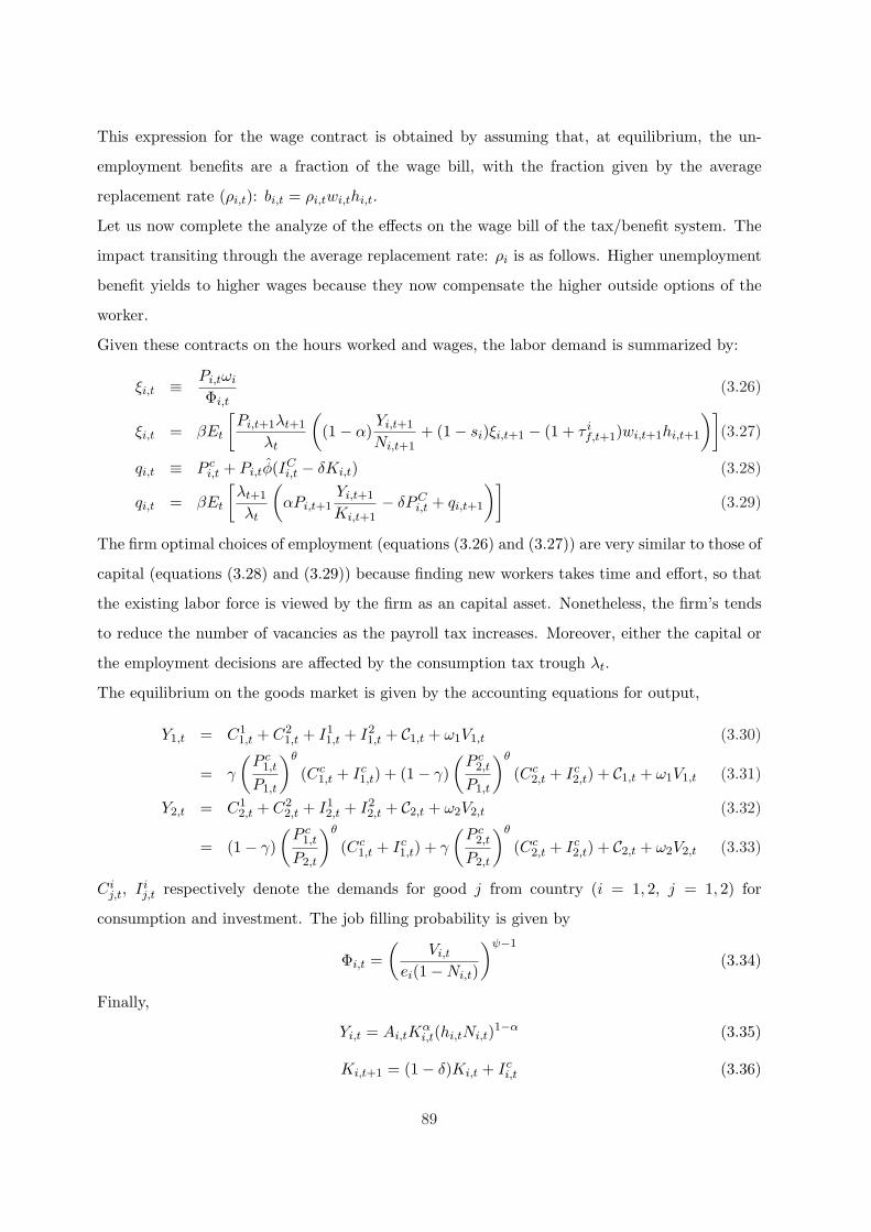
This expression for the wage contract is obtained by assuming that, at equilibrium, the un-
employment benefits are a fraction of the wage bill, with the fraction given by the average
replacement rate (ρi,t): bi,t = ρi,twi,thi,t.
Let us now complete the analyze of the effects on the wage bill of the tax/benefit system. The
impact transiting through the average replacement rate: ρi is as follows. Higher unemployment
benefit yields to higher wages because they now compensate the higher outside options of the
worker.
Given these contracts on the hours worked and wages, the labor demand is summarized by:
ξi,t ≡ Pi,tωi
Φi,t(3.26)
ξi,t = βEt
[Pi,t+1λt+1
λt
((1− α)
Yi,t+1
Ni,t+1+ (1− si)ξi,t+1 − (1 + τ i
f,t+1)wi,t+1hi,t+1
)](3.27)
qi,t ≡ P ci,t + Pi,tφ(IC
i,t − δKi,t) (3.28)
qi,t = βEt
[λt+1
λt
(αPi,t+1
Yi,t+1
Ki,t+1− δPC
i,t + qi,t+1
)](3.29)
The firm optimal choices of employment (equations (3.26) and (3.27)) are very similar to those of
capital (equations (3.28) and (3.29)) because finding new workers takes time and effort, so that
the existing labor force is viewed by the firm as an capital asset. Nonetheless, the firm’s tends
to reduce the number of vacancies as the payroll tax increases. Moreover, either the capital or
the employment decisions are affected by the consumption tax trough λt.
The equilibrium on the goods market is given by the accounting equations for output,
Y1,t = C11,t + C2
1,t + I11,t + I2
1,t + C1,t + ω1V1,t (3.30)
= γ
(P c
1,t
P1,t
)θ
(Cc1,t + Ic
1,t) + (1− γ)(
P c2,t
P1,t
)θ
(Cc2,t + Ic
2,t) + C1,t + ω1V1,t (3.31)
Y2,t = C12,t + C2
2,t + I12,t + I2
2,t + C2,t + ω2V2,t (3.32)
= (1− γ)(
P c1,t
P2,t
)θ
(Cc1,t + Ic
1,t) + γ
(P c
2,t
P2,t
)θ
(Cc2,t + Ic
2,t) + C2,t + ω2V2,t (3.33)
Cij,t, Ii
j,t respectively denote the demands for good j from country (i = 1, 2, j = 1, 2) for
consumption and investment. The job filling probability is given by
Φi,t =(
Vi,t
ei(1−Ni,t)
)ψ−1
(3.34)
Finally,
Yi,t = Ai,tKαi,t(hi,tNi,t)1−α (3.35)
Ki,t+1 = (1− δ)Ki,t + Ici,t (3.36)
89
3.2 Empirical results
As we aim to shed new light on old debates, for numerous parameters, as well as for the stylized
facts, we use standard values. The most taken from the Backus, Kehoe, and Kydland (1994)’ and
Andolfatto (1996)’ works. We also adopt a symmetrical calibration between the two countries
with a null net exports steady state. This facilitates the comparison of our results with a bulk
of previous literature on international fluctuations. For the additional parameters, in particular
those regarding taxes, the procedure for calibrating is quiet traditional. However, matter of
consistency, estimations and average values are based on the 1970:1-1986:4 period, as in Backus
et al.(1994).
3.2.1 Parameterization
The technology parameters are calibrated as follows (Backus et al.(1994)). The autocorrelation
parameter ρ1,1 = ρ2,2 = ρ is set at 0.906. The cross-country diffusion parameter ρ1,2 = ρ2,1 = ρ∗
is fixed at 0.088 and υ1,2 = υ2,1 = υ is calibrated in order to get a correlation between technology
innovations of 0.258. The depreciation rate δ is set at 0.025. α, which no longer corresponds to
the labor share of output, is calibrated in order to get a labor share of 64%.
Following Backus et al.(1994), θ, the elasticity of substitution between domestic and foreign
goods, is set at 1.5, while the discount factor β is set at 0.99. The value of the home bias γ
is set at 0.85. The capital adjustment cost parameter, φ is calibrated in order to replicate the
volatility of investment in each model configuration.
For the labor-market parameters, the calibration is symmetric across countries and rely mostly
on (Andolfatto 1996). The elasticity of the matching function with respect to vacancies and the
firm’s bargaining power are set to ε = ψ = 0.6. The value of χ is chosen to be consistent with
the stationary values (in the non-taxation economy) for the probability that a vacancy position
becomes a productive job, the employment ratio and the fraction of time spent working: Φ = 0.9,
N = 0.57 and h = 1/3. The ratio of aggregate recruiting expenditures to output is fixed at
ωV ∗/Y ∗ = 1%, and the average fraction of time that nonemployed households devote to search
to e = h∗/2. Following Hairault (2002), we choose η = 5 and the quarterly rate of transition from
employment to non-employment equal to s = 0.10. Lastly, parameters σ and Γu are computed
to be consistent with steady-state restrictions.
The last set of values concerns the evolution of the tax rates (equation 3.12). We estimate the
90
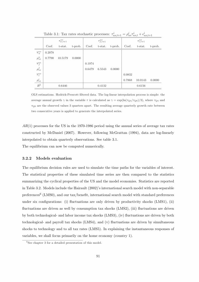
Table 3.1: Tax rates stochastic processes: τ ius,t+1 = ρi
usτius,t + εi
us,t+1
τusw,t+1 τus
f,t+1 τusc,t+1
Coef. t-stat. t-prob. Coef. t-stat. t-prob. Coef. t-stat. t-prob.
τusw 0.2078
ρwus 0.7790 10.5179 0.0000
τusf 0.1974
ρfus 0.6479 6.5543 0.0000
τusc 0.0832
ρcus 0.7868 10.0143 0.0000
R2 0.6446 0.4132 0.6156
OLS estimations. Hodrick-Prescott filtered data. The log-linear interpolation process is simple: the
average annual growth γ in the variable τ is calculated as γ = exp(ln(τQ4/τQ0)/3), where τQ4 and
τQ0 are the observed values 3 quarters apart. The resulting average quarterly growth rate between
two consecutive years is applied to generate the interpolated series.
AR(1) processes for the US in the 1970-1986 period using the annual series of average tax rates
constructed by McDaniel (2007). However, following McGrattan (1994), data are log-linearly
interpolated to obtain quarterly observations. See table 3.1.
The equilibrium can now be computed numerically.
3.2.2 Models evaluation
The equilibrium decision rules are used to simulate the time paths for the variables of interest.
The statistical properties of these simulated time series are then compared to the statistics
summarizing the cyclical properties of the US and the model economies. Statistics are reported
in Table 3.2. Models include the Hairault (2002)’s international search model with non-separable
preferences6 (LMS0), and our tax/benefit, international search model with standard preferences
under six configurations: (i) fluctuations are only driven by productivity shocks (LMS1), (ii)
fluctuations are driven as well by consumption tax shocks (LMS2), (iii) fluctuations are driven
by both technological- and labor income tax shocks (LMS3), (iv) fluctuations are driven by both
technological- and payroll tax shocks (LMS4), and (v) fluctuations are driven by simultaneous
shocks to technology and to all tax rates (LMS5). In explaining the instantaneous responses of
variables, we shall focus primarily on the home economy (country 1).6See chapter 3 for a detailed presentation of this model.
91
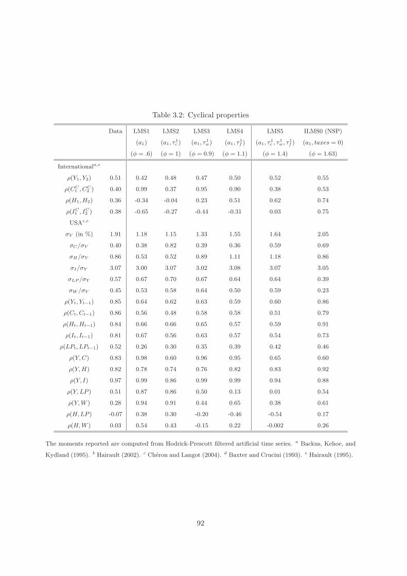
Table 3.2: Cyclical properties
Data LMS1 LMS2 LMS3 LMS4 LMS5 ILMS0 (NSP)
(a1) (a1, τ1c ) (a1, τ
1w) (a1, τ
1f ) (a1, τ
1c , τ1
w, τ1f ) (a1, taxes = 0)
(φ = .6) (φ = 1) (φ = 0.9) (φ = 1.1) (φ = 1.4) (φ = 1.63)
Internationala,e
ρ(Y1, Y2) 0.51 0.42 0.48 0.47 0.50 0.52 0.55
ρ(CC1 , CC
2 ) 0.40 0.99 0.37 0.95 0.90 0.38 0.53
ρ(H1, H2) 0.36 -0.34 -0.04 0.23 0.51 0.62 0.74
ρ(IC1 , IC
2 ) 0.38 -0.65 -0.27 -0.44 -0.31 0.03 0.75
USAc,e
σY (in %) 1.91 1.18 1.15 1.33 1.55 1.64 2.05
σC/σY 0.40 0.38 0.82 0.39 0.36 0.59 0.69
σH/σY 0.86 0.53 0.52 0.89 1.11 1.18 0.86
σI/σY 3.07 3.00 3.07 3.02 3.08 3.07 3.05
σLP /σY 0.57 0.67 0.70 0.67 0.64 0.64 0.39
σW /σY 0.45 0.53 0.58 0.64 0.50 0.59 0.23
ρ(Yt, Yt−1) 0.85 0.64 0.62 0.63 0.59 0.60 0.86
ρ(Ct, Ct−1) 0.86 0.56 0.48 0.58 0.58 0.51 0.79
ρ(Ht, Ht−1) 0.84 0.66 0.66 0.65 0.57 0.59 0.91
ρ(It, It−1) 0.81 0.67 0.56 0.63 0.57 0.54 0.73
ρ(LPt, LPt−1) 0.52 0.26 0.30 0.35 0.39 0.42 0.46
ρ(Y, C) 0.83 0.98 0.60 0.96 0.95 0.65 0.60
ρ(Y, H) 0.82 0.78 0.74 0.76 0.82 0.83 0.92
ρ(Y, I) 0.97 0.99 0.86 0.99 0.99 0.94 0.88
ρ(Y, LP ) 0.51 0.87 0.86 0.50 0.13 0.01 0.54
ρ(Y, W ) 0.28 0.94 0.91 0.44 0.65 0.38 0.61
ρ(H, LP ) -0.07 0.38 0.30 -0.20 -0.46 -0.54 0.17
ρ(H, W ) 0.03 0.54 0.43 -0.15 0.22 -0.002 0.26
The moments reported are computed from Hodrick-Prescott filtered artificial time series. a Backus, Kehoe, and
Kydland (1995). b Hairault (2002). c Cheron and Langot (2004). d Baxter and Crucini (1993). e Hairault (1995).
92
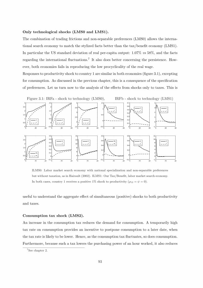
Only technological shocks (LMS0 and LMS1).
The combination of trading frictions and non-separable preferences (LMS0) allows the interna-
tional search economy to match the stylized facts better than the tax/benefit economy (LMS1).
In particular the US standard deviation of real per-capita output: 1.07% vs 58%, and the facts
regarding the international fluctuations.7 It also does better concerning the persistence. How-
ever, both economies fails in reproducing the low procyclicality of the real wage.
Responses to productivity shock to country 1 are similar in both economies (figure 3.1), excepting
for consumption. As discussed in the previous chapter, this is a consequence of the specification
of preferences. Let us turn now to the analysis of the effects from shocks only to taxes. This is
Figure 3.1: IRFa - shock to technology (LMS0), IRFb - shock to technology (LMS1)
0 20 400
0.5
1
1.5
2
2.5
3
Y1
Y2
0 20 40−0.5
0
0.5
1
1.5
2
2.5
C1
C2
0 20 401.5
2
2.5
3
3.5
4
I1
I2
0 20 400
0.5
1
1.5
2
2.5
3
Nh1
Nh2
0 20 40−0.1
0
0.1
0.2
0.3
0.4
0.5
0.6
w1
w2
0 20 402
4
6
8
10
12
14
V1
V2
0 20 40−0.5
0
0.5
1
1.5
Y1
Y2
0 20 400
0.1
0.2
0.3
0.4
0.5
0.6
0.7
C1
C2
0 20 40−1
0
1
2
3
4
I1
I2
0 20 40−0.2
0
0.2
0.4
0.6
0.8
Nh1
Nh2
0 20 40−0.2
0
0.2
0.4
0.6
0.8
w1
w2
0 20 40−2
0
2
4
6
8
10
12
V1
V2
ILMS0: Labor market search economy with national specialization and non-separable preferences
but without taxation, as in Hairault (2002). ILMS1: Our Tax/Benefit, labor market search economy.
In both cases, country 1 receives a positive 1% shock to productivity (ρ12 = ψ = 0).
useful to understand the aggregate effect of simultaneous (positive) shocks to both productivity
and taxes.
Consumption tax shock (LMS2).
An increase in the consumption tax reduces the demand for consumption. A temporarily high
tax rate on consumption provides an incentive to postpone consumption to a later date, when
the tax rate is likely to be lower. Hence, as the consumption tax fluctuates, so does consumption.
Furthermore, because such a tax lowers the purchasing power of an hour worked, it also reduces7See chapter 2.
93
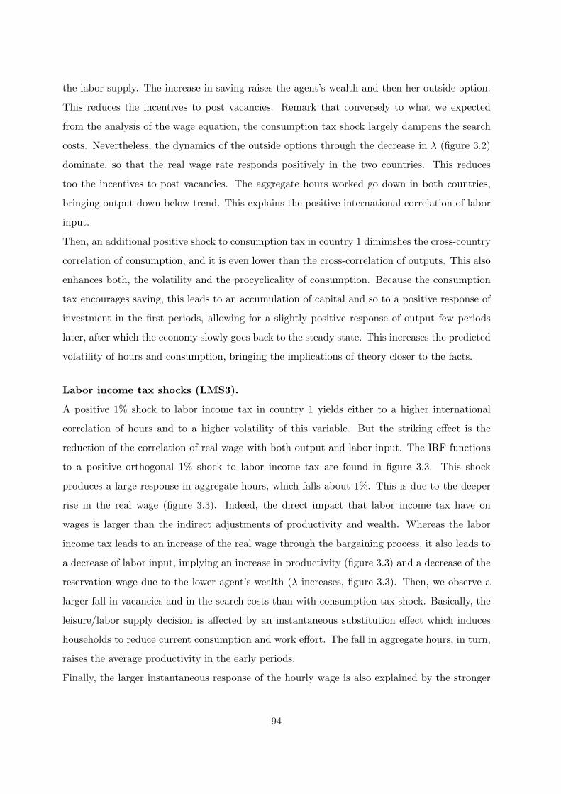
the labor supply. The increase in saving raises the agent’s wealth and then her outside option.
This reduces the incentives to post vacancies. Remark that conversely to what we expected
from the analysis of the wage equation, the consumption tax shock largely dampens the search
costs. Nevertheless, the dynamics of the outside options through the decrease in λ (figure 3.2)
dominate, so that the real wage rate responds positively in the two countries. This reduces
too the incentives to post vacancies. The aggregate hours worked go down in both countries,
bringing output down below trend. This explains the positive international correlation of labor
input.
Then, an additional positive shock to consumption tax in country 1 diminishes the cross-country
correlation of consumption, and it is even lower than the cross-correlation of outputs. This also
enhances both, the volatility and the procyclicality of consumption. Because the consumption
tax encourages saving, this leads to an accumulation of capital and so to a positive response of
investment in the first periods, allowing for a slightly positive response of output few periods
later, after which the economy slowly goes back to the steady state. This increases the predicted
volatility of hours and consumption, bringing the implications of theory closer to the facts.
Labor income tax shocks (LMS3).
A positive 1% shock to labor income tax in country 1 yields either to a higher international
correlation of hours and to a higher volatility of this variable. But the striking effect is the
reduction of the correlation of real wage with both output and labor input. The IRF functions
to a positive orthogonal 1% shock to labor income tax are found in figure 3.3. This shock
produces a large response in aggregate hours, which falls about 1%. This is due to the deeper
rise in the real wage (figure 3.3). Indeed, the direct impact that labor income tax have on
wages is larger than the indirect adjustments of productivity and wealth. Whereas the labor
income tax leads to an increase of the real wage through the bargaining process, it also leads to
a decrease of labor input, implying an increase in productivity (figure 3.3) and a decrease of the
reservation wage due to the lower agent’s wealth (λ increases, figure 3.3). Then, we observe a
larger fall in vacancies and in the search costs than with consumption tax shock. Basically, the
leisure/labor supply decision is affected by an instantaneous substitution effect which induces
households to reduce current consumption and work effort. The fall in aggregate hours, in turn,
raises the average productivity in the early periods.
Finally, the larger instantaneous response of the hourly wage is also explained by the stronger
94
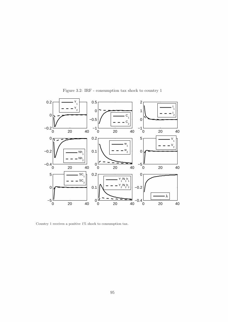
Figure 3.2: IRF - consumption tax shock to country 1
0 20 40−0.2
0
0.2
Y1
Y2
0 20 40−1
−0.5
0
0.5
C1
C2
0 20 40−1
0
1
2
I1
I2
0 20 40−0.4
−0.2
0
Nh1
Nh2
0 20 400
0.1
0.2
w
1
w2
0 20 40−5
0
5
V1
V2
0 20 40−5
0
5
SC1
SC2
0 20 400
0.1
0.2
Y
1/N
1h
1
Y2/N
2h
2
0 20 40−0.4
−0.2
0
λ
Country 1 receives a positive 1% shock to consumption tax.
95
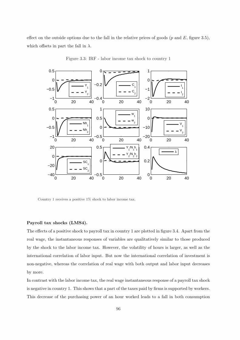
effect on the outside options due to the fall in the relative prices of goods (p and E, figure 3.5),
which offsets in part the fall in λ.
Figure 3.3: IRF - labor income tax shock to country 1
0 20 40−1
−0.5
0
0.5
Y1
Y2
0 20 40−0.4
−0.2
0
C1
C2
0 20 40−2
−1
0
1
I1
I2
0 20 40−1
−0.5
0
0.5
Nh1
Nh2
0 20 40−0.5
0
0.5
1
w
1
w2
0 20 40−20
−10
0
10
V1
V2
0 20 40−40
−20
0
20
SC1
SC2
0 20 40−0.5
0
0.5
Y1/N
1h
1
Y2/N
2h
2
0 20 400
0.2
0.4
λ
Country 1 receives a positive 1% shock to labor income tax.
Payroll tax shocks (LMS4).
The effects of a positive shock to payroll tax in country 1 are plotted in figure 3.4. Apart from the
real wage, the instantaneous responses of variables are qualitatively similar to those produced
by the shock to the labor income tax. However, the volatility of hours is larger, as well as the
international correlation of labor input. But now the international correlation of investment is
non-negative, whereas the correlation of real wage with both output and labor input decreases
by more.
In contrast with the labor income tax, the real wage instantaneous response of a payroll tax shock
is negative in country 1. This shows that a part of the taxes paid by firms is supported by workers.
This decrease of the purchasing power of an hour worked leads to a fall in both consumption
96
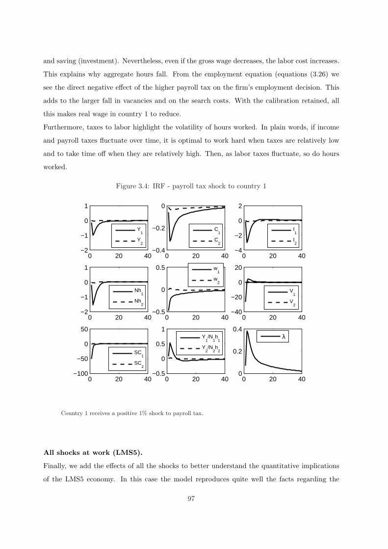
and saving (investment). Nevertheless, even if the gross wage decreases, the labor cost increases.
This explains why aggregate hours fall. From the employment equation (equations (3.26) we
see the direct negative effect of the higher payroll tax on the firm’s employment decision. This
adds to the larger fall in vacancies and on the search costs. With the calibration retained, all
this makes real wage in country 1 to reduce.
Furthermore, taxes to labor highlight the volatility of hours worked. In plain words, if income
and payroll taxes fluctuate over time, it is optimal to work hard when taxes are relatively low
and to take time off when they are relatively high. Then, as labor taxes fluctuate, so do hours
worked.
Figure 3.4: IRF - payroll tax shock to country 1
0 20 40−2
−1
0
1
Y1
Y2
0 20 40−0.4
−0.2
0
C1
C2
0 20 40−4
−2
0
2
I1
I2
0 20 40−2
−1
0
1
Nh1
Nh2
0 20 40−0.5
0
0.5
w1
w2
0 20 40−40
−20
0
20
V1
V2
0 20 40−100
−50
0
50
SC1
SC2
0 20 40−0.5
0
0.5
1
Y
1/N
1h
1
Y2/N
2h
2
0 20 400
0.2
0.4
λ
Country 1 receives a positive 1% shock to payroll tax.
All shocks at work (LMS5).
Finally, we add the effects of all the shocks to better understand the quantitative implications
of the LMS5 economy. In this case the model reproduces quite well the facts regarding the
97
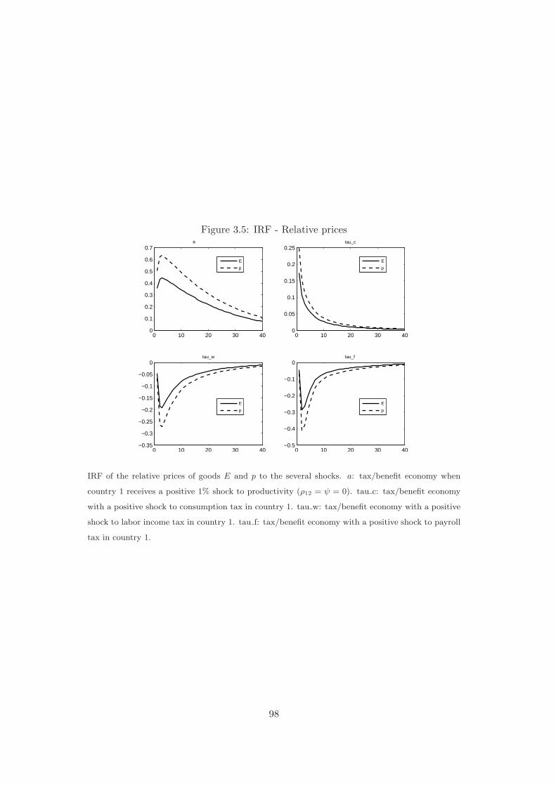
Figure 3.5: IRF - Relative prices
0 10 20 30 400
0.1
0.2
0.3
0.4
0.5
0.6
0.7a
E
p
0 10 20 30 400
0.05
0.1
0.15
0.2
0.25tau_c
E
p
0 10 20 30 40−0.35
−0.3
−0.25
−0.2
−0.15
−0.1
−0.05
0tau_w
E
p
0 10 20 30 40−0.5
−0.4
−0.3
−0.2
−0.1
0tau_f
E
p
IRF of the relative prices of goods E and p to the several shocks. a: tax/benefit economy when
country 1 receives a positive 1% shock to productivity (ρ12 = ψ = 0). tau c: tax/benefit economy
with a positive shock to consumption tax in country 1. tau w: tax/benefit economy with a positive
shock to labor income tax in country 1. tau f: tax/benefit economy with a positive shock to payroll
tax in country 1.
98
international comovements, because the consumption tax allows to reduce the international
correlation of consumption, whereas the two production inputs (aggregate hours and investment)
are now positively correlated, contrary two the model with only technological shock.
Concerning the labor market dynamics, the introduction of fiscal shocks allows to significantly
reduce the correlation of wages with the output and the aggregate hours (the Dunlop-Tarshis
puzzle). The model allows to match the relative volatility of real wages. However, the relative
standard deviation of hours is slightly overstated. Nevertheless, results are encouraging.
3.3 Conclusion
In this chapter the effects of distortionary taxation are studied in the context of a two-country
general equilibrium model with search and matching on the labor market. We show that dis-
tortive taxes on labor and consumption have important effects on the quantitative properties of
the model, allowing to outperform the predictions from the model without taxation in several
lines. In particular, we show that the fluctuations in distortive taxes provide a plausive explana-
tion from the three empirical puzzles concerning the real wage dynamics and the international
fluctuations.
Moreover, our framework reconciliate the standard separable preferences with either the observed
U.S. real wage rigidity and the international fluctuations, by taking into account the tax/benefyt
system. This provides simultaneously an explanation to the real wage rigidity puzzle, alternative
to that of Cheron and Langot (2004); and an explanation to the quantities puzzle (concerning
the ranking of the outputs correlation relative to the consumptions correlation), alternative to
the Hairault (2002)’s one. In the two cases, the authors base their explanation on the non-
separability of agents’ preferences between consumption and leisure.
Nevertheless, the problem of modelling income taxes has not been resolved in a fully satisfactory
way. The volatility of labor input is exaggerated, whereas the persistence of output and the other
macro aggregates is underestimated. Despite our model’s shortcomings, it is striking how much
we are able to explain by amending a basic two-country search model with fairly standard
preferences to include fiscal policy variables.
99

Chapter 4
Growth, Unemployment and
Tax/Benefit system in European
Countries
This chapter is in part based on a joint working paper with Stephane Adjemian and Francois
Langot (European Commission, TAXBEN SCS8-CT-2004-502639, 2006.)
100
Introduction
The observed high unemployment in continental Europe and the slowdown in economic growth
in the last decades naturally raise the question of whether these two phenomena are related. On
the empirical side, there is no consensus regarding the sign of the correlation between growth
and unemployment, either across countries or over time within a country.1 The same is true
on the theoretical side.2 Nevertheless, the endogenous growth theory predicts that distortions
due to fiscal instruments lead to a lower growth whereas the equilibrium unemployment theory
predicts that these distortions lead to a higher unemployment rate. This suggests that the link
between growth and unemployment can be viewed through the simultaneous link of growth and
unemployment with the labor market institutions.
In this chapter we investigate the issue of the long run link between growth and unemployment
at two levels. First, we conduct an empirical analysis to we explore the heterogeneity of growth
and unemployment experiences across 183 European regions and we evaluate how much of this
heterogeneity is accounted by the national labor market institutions. The originality of this
approach is to take into account the large heterogeneity between regions among a country. Sec-
ond, we construct a theoretical economy to assess the explicative role of labor-market variables
on the bad performance of European countries. The main hypotheses of our model are the fol-
lowing: (i) Innovations are the engine of growth. This implies a “creative destruction” process
generating jobs reallocation. (ii) Agents have the choice of being employed or being trying their
hand at R&D; and (iii) Unemployment is caused both by the wage-setting behavior of unions,
and by the labor costs associated to the tax/benefit system.3 In addition, in the appendix to
this chapter, we conduct a social welfare exercise using a simplified version of this model.
The advises from the empirical exercise are that: (i) The tax wedge and the unemployment
benefits are positively correlated with the regional unemployment rates. Conversely, the em-
ployment protection and the level of coordination in the wage bargaining process are negatively
correlated with the regional unemployment rates. (ii) The tax wedge and the unemployment1See Mortensen (2005) for a wide review of the empirical literature, which shows the diversity of results about
the correlation between growth and unemployment.2This is due to the offsetting nature of two main effects: a higher rate of growth in productivity will reduce
unemployment trough a positive “capitalization” effect on investment in job creation; whereas the “creative
destruction effect”, inherent to the growth process, leads to a faster obsolescence of technologies and so to a faster
rate of job destruction.3The two first hypotheses are the same as those of Aghion and Howitt (1994).
101
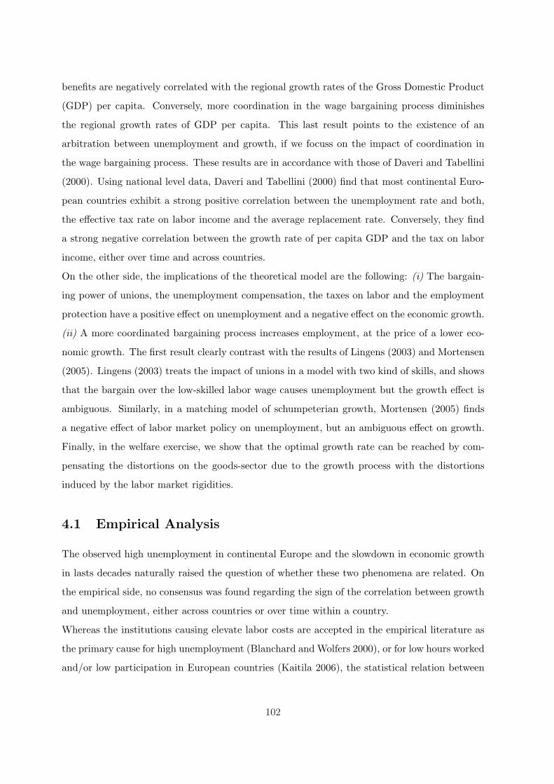
benefits are negatively correlated with the regional growth rates of the Gross Domestic Product
(GDP) per capita. Conversely, more coordination in the wage bargaining process diminishes
the regional growth rates of GDP per capita. This last result points to the existence of an
arbitration between unemployment and growth, if we focuss on the impact of coordination in
the wage bargaining process. These results are in accordance with those of Daveri and Tabellini
(2000). Using national level data, Daveri and Tabellini (2000) find that most continental Euro-
pean countries exhibit a strong positive correlation between the unemployment rate and both,
the effective tax rate on labor income and the average replacement rate. Conversely, they find
a strong negative correlation between the growth rate of per capita GDP and the tax on labor
income, either over time and across countries.
On the other side, the implications of the theoretical model are the following: (i) The bargain-
ing power of unions, the unemployment compensation, the taxes on labor and the employment
protection have a positive effect on unemployment and a negative effect on the economic growth.
(ii) A more coordinated bargaining process increases employment, at the price of a lower eco-
nomic growth. The first result clearly contrast with the results of Lingens (2003) and Mortensen
(2005). Lingens (2003) treats the impact of unions in a model with two kind of skills, and shows
that the bargain over the low-skilled labor wage causes unemployment but the growth effect is
ambiguous. Similarly, in a matching model of schumpeterian growth, Mortensen (2005) finds
a negative effect of labor market policy on unemployment, but an ambiguous effect on growth.
Finally, in the welfare exercise, we show that the optimal growth rate can be reached by com-
pensating the distortions on the goods-sector due to the growth process with the distortions
induced by the labor market rigidities.
4.1 Empirical Analysis
The observed high unemployment in continental Europe and the slowdown in economic growth
in lasts decades naturally raised the question of whether these two phenomena are related. On
the empirical side, no consensus was found regarding the sign of the correlation between growth
and unemployment, either across countries or over time within a country.
Whereas the institutions causing elevate labor costs are accepted in the empirical literature as
the primary cause for high unemployment (Blanchard and Wolfers 2000), or for low hours worked
and/or low participation in European countries (Kaitila 2006), the statistical relation between
102
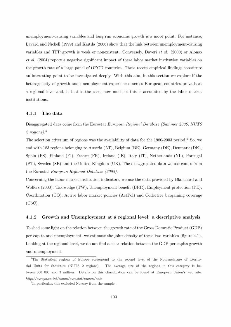
unemployment-causing variables and long run economic growth is a moot point. For instance,
Layard and Nickell (1999) and Kaitila (2006) show that the link between unemployment-causing
variables and TFP growth is weak or nonexistent. Conversely, Daveri et al. (2000) or Alonso
et al. (2004) report a negative significant impact of these labor market institution variables on
the growth rate of a large panel of OECD countries. These recent empirical findings constitute
an interesting point to be investigated deeply. With this aim, in this section we explore if the
heterogeneity of growth and unemployment experiences across European countries prevails at
a regional level and, if that is the case, how much of this is accounted by the labor market
institutions.
4.1.1 The data
Disaggregated data come from the Eurostat European Regional Database (Summer 2006, NUTS
2 regions).4
The selection criterium of regions was the availability of data for the 1980-2003 period.5 So, we
end with 183 regions belonging to Austria (AT), Belgium (BE), Germany (DE), Denmark (DK),
Spain (ES), Finland (FI), France (FR), Ireland (IE), Italy (IT), Netherlands (NL), Portugal
(PT), Sweden (SE) and the United Kingdom (UK). The disaggregated data we use comes from
the Eurostat European Regional Database (2005).
Concerning the labor market institution indicators, we use the data provided by Blanchard and
Wolfers (2000): Tax wedge (TW), Unemployment benefit (BRR), Employment protection (PE),
Coordination (CO), Active labor market policies (ActPol) and Collective bargaining coverage
(CbC).
4.1.2 Growth and Unemployment at a regional level: a descriptive analysis
To shed some light on the relation between the growth rate of the Gross Domestic Product (GDP)
per capita and unemployment, we estimate the joint density of these two variables (figure 4.1).
Looking at the regional level, we do not find a clear relation between the GDP per capita growth
and unemployment.4The Statistical regions of Europe correspond to the second level of the Nomenclature of Territo-
rial Units for Statistics (NUTS 2 regions). The average size of the regions in this category is be-
tween 800 000 and 3 million. Details on this classification can be found at European Union’s web site:
http://europa.eu.int/comm/eurostat/ramon/nuts5In particular, this excluded Norway from the sample.
103
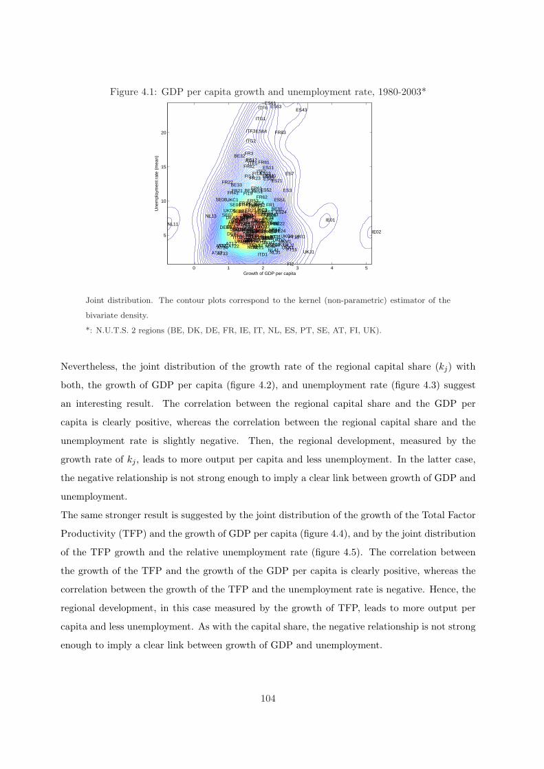
Figure 4.1: GDP per capita growth and unemployment rate, 1980-2003*
Growth of GDP per capita
Une
mpl
oym
ent r
ate
(mea
n)
DK01
DK02
DK03
BE1
BE21
BE22BE23
BE24
BE25
BE31
BE32
BE33
BE34
BE35
DE11DE12
DE13DE14
DE21
DE22DE23
DE24DE25DE26
DE27
DE5
DE6DE71
DE72DE73DE91
DE92DE93
DE94DEA1
DEA2DEA3
DEA4
DEA5
DEB1DEB2
DEB3DECDEF
SE01
SE02SE04
SE06
SE07
SE08
SE09SE0A
FR1
FR21
FR22FR23
FR24
FR25FR26
FR3
FR41
FR42
FR43
FR51
FR52FR53
FR61
FR62
FR63FR71FR72
FR81FR82
FR83
IE01
IE02
ITC1
ITC2
ITC3
ITC4
ITD1
ITD2ITD3
ITD4ITD5
ITE1ITE2
ITE3
ITE4
ITF1
ITF2
ITF3
ITF4ITF5
ITF6
ITG1
ITG2
NL11
NL12
NL13
NL21NL22NL31
NL32NL33
NL34
NL41NL42
FI13
FI18
FI19
FI1A
FI2
ES11
ES12
ES13
ES21
ES22ES23 ES24
ES3
ES41ES42
ES43
ES51
ES52
ES53
ES61
ES62
ES63
ES64
ES7
PT11
PT16
PT17PT18
PT15AT11
AT12
AT13
AT21AT22AT31
AT32AT33AT34
UKC1
UKC2
UKD1
UKD2
UKD3
UKD4
UKD5UKE1
UKE2
UKE3
UKE4UKF1UKF2UKF3 UKG1
UKG2UKG3
UKH1UKH2
UKH3 UKI1
UKI2
UKJ1UKJ2
UKJ3UKJ4
UKK1
UKK2
UKK3
UKK4
UKL1
UKL2
UKM1
UKM2
UKM3UKM4
UKN
0 1 2 3 4 5
5
10
15
20
Joint distribution. The contour plots correspond to the kernel (non-parametric) estimator of the
bivariate density.
*: N.U.T.S. 2 regions (BE, DK, DE, FR, IE, IT, NL, ES, PT, SE, AT, FI, UK).
Nevertheless, the joint distribution of the growth rate of the regional capital share (kj) with
both, the growth of GDP per capita (figure 4.2), and unemployment rate (figure 4.3) suggest
an interesting result. The correlation between the regional capital share and the GDP per
capita is clearly positive, whereas the correlation between the regional capital share and the
unemployment rate is slightly negative. Then, the regional development, measured by the
growth rate of kj , leads to more output per capita and less unemployment. In the latter case,
the negative relationship is not strong enough to imply a clear link between growth of GDP and
unemployment.
The same stronger result is suggested by the joint distribution of the growth of the Total Factor
Productivity (TFP) and the growth of GDP per capita (figure 4.4), and by the joint distribution
of the TFP growth and the relative unemployment rate (figure 4.5). The correlation between
the growth of the TFP and the growth of the GDP per capita is clearly positive, whereas the
correlation between the growth of the TFP and the unemployment rate is negative. Hence, the
regional development, in this case measured by the growth of TFP, leads to more output per
capita and less unemployment. As with the capital share, the negative relationship is not strong
enough to imply a clear link between growth of GDP and unemployment.
104
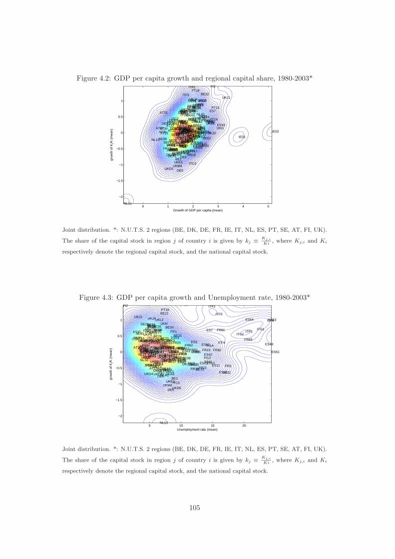
Figure 4.2: GDP per capita growth and regional capital share, 1980-2003*
Growth of GDP per capita (mean)
grow
th o
f Ki/K
(m
ean)
DK01
DK02DK03
BE1
BE21
BE22
BE23BE24
BE25
BE31
BE32BE33
BE34
BE35
DE11DE12DE13DE14
DE21DE22DE23
DE24DE25
DE26DE27
DE5
DE6
DE71
DE72DE73
DE91DE92
DE93DE94
DEA1
DEA2DEA3DEA4
DEA5
DEB1DEB2DEB3
DEC
DEF
SE01
SE02SE04
SE06SE07SE08
SE09SE0A FR1
FR21FR22
FR23FR24
FR25
FR26
FR3FR41
FR42
FR43
FR51FR52FR53FR61
FR62
FR63
FR71
FR72
FR81
FR82
FR83
IE01
IE02
ITC1
ITC2
ITC3
ITC4
ITD1
ITD2
ITD3
ITD4
ITD5
ITE1
ITE2ITE3
ITE4
ITF1
ITF2
ITF3
ITF4
ITF5
ITF6
ITG1
ITG2
NL11
NL12
NL13NL21
NL22
NL31
NL32
NL33
NL34NL41
NL42
FI13
FI18
FI19
FI1A
FI2
ES11
ES12
ES13ES21
ES22ES23
ES24
ES3
ES41
ES42
ES43
ES51ES52
ES53
ES61
ES62
ES63ES64
ES7
PT11
PT16
PT17
PT18
PT15
AT11
AT12
AT13
AT21AT22AT31
AT32
AT33
AT34
UKC1
UKC2UKD1
UKD2
UKD3UKD4
UKD5
UKE1 UKE2
UKE3
UKE4UKF1
UKF2
UKF3
UKG1
UKG2
UKG3
UKH1
UKH2UKH3UKI1UKI2
UKJ1
UKJ2
UKJ3
UKJ4
UKK1UKK2UKK3
UKK4
UKL1
UKL2
UKM1
UKM2
UKM3
UKM4
UKN
0 1 2 3 4 5
−2
−1.5
−1
−0.5
0
0.5
1
Joint distribution. *: N.U.T.S. 2 regions (BE, DK, DE, FR, IE, IT, NL, ES, PT, SE, AT, FI, UK).
The share of the capital stock in region j of country i is given by kj ≡ Kj,i
Ki, where Kj,i and Ki
respectively denote the regional capital stock, and the national capital stock.
Figure 4.3: GDP per capita growth and Unemployment rate, 1980-2003*
Unemployment rate (mean)
grow
th o
f Ki/K
(m
ean)
DK01
DK02DK03
BE1
BE21
BE22
BE23BE24
BE25
BE31
BE32BE33
BE34
BE35
DE11DE12DE13DE14
DE21DE22DE23
DE24DE25
DE26DE27
DE5
DE6
DE71
DE72DE73
DE91DE92
DE93DE94
DEA1
DEA2DEA3DEA4
DEA5
DEB1DEB2DEB3
DEC
DEF
SE01
SE02SE04
SE06SE07SE08
SE09SE0A FR1
FR21FR22
FR23FR24
FR25
FR26
FR3FR41
FR42
FR43
FR51FR52FR53FR61
FR62
FR63
FR71
FR72
FR81
FR82
FR83
IE01
IE02
ITC1
ITC2
ITC3
ITC4
ITD1
ITD2
ITD3
ITD4
ITD5
ITE1
ITE2ITE3
ITE4
ITF1
ITF2
ITF3
ITF4
ITF5
ITF6
ITG1
ITG2
NL11
NL12
NL13NL21NL22
NL31
NL32
NL33
NL34NL41
NL42
FI13
FI18
FI19
FI1A
FI2
ES11
ES12
ES13ES21
ES22ES23
ES24
ES3
ES41
ES42
ES43
ES51 ES52
ES53
ES61
ES62
ES63ES64
ES7
PT11
PT16
PT17
PT18
PT15
AT11
AT12
AT13
AT21AT22AT31
AT32
AT33
AT34
UKC1
UKC2UKD1
UKD2
UKD3UKD4
UKD5
UKE1UKE2
UKE3
UKE4UKF1
UKF2
UKF3
UKG1
UKG2
UKG3
UKH1
UKH2UKH3UKI1 UKI2
UKJ1
UKJ2
UKJ3
UKJ4
UKK1UKK2 UKK3
UKK4
UKL1
UKL2
UKM1
UKM2
UKM3
UKM4
UKN
5 10 15 20
−2
−1.5
−1
−0.5
0
0.5
1
Joint distribution. *: N.U.T.S. 2 regions (BE, DK, DE, FR, IE, IT, NL, ES, PT, SE, AT, FI, UK).
The share of the capital stock in region j of country i is given by kj ≡ Kj,i
Ki, where Kj,i and Ki
respectively denote the regional capital stock, and the national capital stock.
105
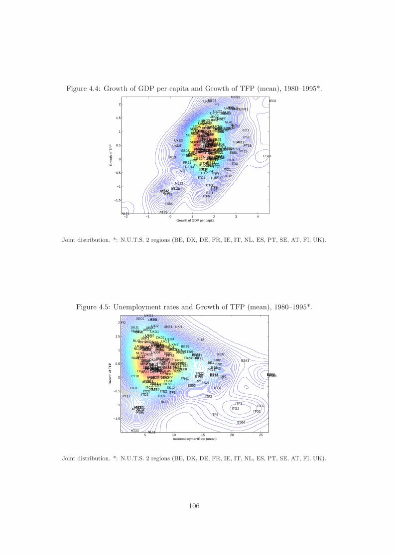
Figure 4.4: Growth of GDP per capita and Growth of TFP (mean), 1980–1995*.
Growth of GDP per capita
Gro
wth
of T
FP
DK01
DK02
DK03BE1
BE21
BE22
BE23
BE24
BE25
BE31
BE32BE33
BE34BE35
DE11DE12
DE13
DE14
DE21DE22DE23DE24
DE25
DE26DE27
DE5DE6
DE71
DE72DE73
DE91
DE92
DE93DE94
DEA1DEA2
DEA3DEA4DEA5
DEB1
DEB2
DEB3
DEC
DEF
SE01
SE02
SE04SE06
SE07
SE08
SE09
SE0AFR1
FR21
FR22
FR23FR24
FR25
FR26
FR3
FR41
FR42FR43
FR51
FR52
FR53
FR61
FR62FR63FR71
FR72
FR81FR82
FR83
IE01
IE02
ITC1
ITC2
ITC3
ITC4
ITD1
ITD2
ITD3ITD4
ITD5
ITE1
ITE2
ITE3
ITE4
ITF1ITF2
ITF3
ITF4
ITF5
ITF6
ITG1ITG2
NL11
NL12
NL13
NL21NL22
NL31
NL32NL33
NL34
NL41
NL42
FI13
FI18
FI19
FI1A
FI2
ES11
ES12
ES13
ES21
ES22ES23
ES24ES3
ES41ES42
ES43
ES51
ES52
ES53
ES61ES62ES63
ES64
ES7
PT11
PT15
PT16
PT17
PT18
AT11AT12
AT13
AT21
AT22AT31
AT32
AT33
AT34
UKC1UKC2
UKD1UKD2
UKD3
UKD4
UKD5
UKE1
UKE2
UKE3
UKE4UKF1
UKF2UKF3
UKG1
UKG2UKG3
UKH1
UKH2
UKH3
UKI1UKI2UKJ1UKJ2
UKJ3 UKJ4UKK1UKK2
UKK3
UKK4
UKL1
UKL2
UKM1
UKM2UKM3
UKM4
UKN
−2 −1 0 1 2 3 4
−1.5
−1
−0.5
0
0.5
1
1.5
2
Joint distribution. *: N.U.T.S. 2 regions (BE, DK, DE, FR, IE, IT, NL, ES, PT, SE, AT, FI, UK).
Figure 4.5: Unemployment rates and Growth of TFP (mean), 1980–1995*.
mUnemploymentRate (mean)
Gro
wth
of T
FP
DK01
DK02
DK03BE1
BE21
BE22
BE23
BE24
BE25
BE31
BE32BE33
BE34 BE35
DE11DE12
DE13
DE14
DE21DE22DE23DE24
DE25
DE26DE27
DE5DE6
DE71
DE72DE73
DE91
DE92
DE93DE94
DEA1DEA2
DEA3DEA4DEA5
DEB1
DEB2
DEB3
DEC
DEF
SE01
SE02
SE04SE06
SE07
SE08
SE09
SE0AFR1
FR21
FR22
FR23FR24
FR25
FR26
FR3
FR41
FR42FR43
FR51
FR52
FR53
FR61
FR62FR63FR71
FR72
FR81FR82
FR83
IE01
IE02
ITC1
ITC2
ITC3
ITC4
ITD1
ITD2
ITD3ITD4
ITD5
ITE1
ITE2
ITE3
ITE4
ITF1ITF2
ITF3
ITF4
ITF5
ITF6
ITG1ITG2
NL11
NL12
NL13
NL21NL22
NL31
NL32NL33
NL34
NL41
NL42
FI13
FI18
FI19
FI1A
FI2
ES11
ES12
ES13
ES21
ES22ES23
ES24 ES3
ES41ES42
ES43
ES51
ES52
ES53
ES61ES62ES63
ES64
ES7
PT11
PT15
PT16
PT17
PT18
AT11AT12
AT13
AT21
AT22AT31
AT32
AT33
AT34
UKC1UKC2
UKD1UKD2
UKD3
UKD4
UKD5
UKE1
UKE2
UKE3
UKE4UKF1
UKF2UKF3
UKG1
UKG2UKG3
UKH1
UKH2
UKH3
UKI1UKI2UKJ1UKJ2
UKJ3UKJ4UKK1UKK2
UKK3
UKK4
UKL1
UKL2
UKM1
UKM2 UKM3
UKM4
UKN
5 10 15 20 25
−1.5
−1
−0.5
0
0.5
1
1.5
2
Joint distribution. *: N.U.T.S. 2 regions (BE, DK, DE, FR, IE, IT, NL, ES, PT, SE, AT, FI, UK).
106
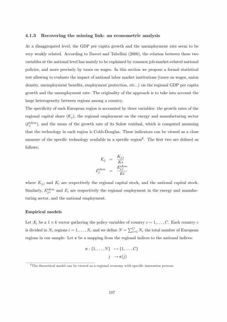
4.1.3 Recovering the missing link: an econometric analysis
At a disaggregated level, the GDP per capita growth and the unemployment rate seem to be
very weakly related. According to Daveri and Tabellini (2000), the relation between these two
variables at the national level has mainly to be explained by common job-market-related national
policies, and more precisely by taxes on wages. In this section we propose a formal statistical
test allowing to evaluate the impact of national labor market institutions (taxes on wages, union
density, unemployment benefits, employment protection, etc...) on the regional GDP per capita
growth and the unemployment rate. The originality of the approach is to take into account the
large heterogeneity between regions among a country.
The specificity of each European region is accounted by three variables: the growth rates of the
regional capital share (Kj), the regional employment on the energy and manufacturing sector
(Ee&mj ), and the mean of the growth rate of its Solow residual, which is computed assuming
that the technology in each region is Cobb-Douglas. These indicators can be viewed as a close
measure of the specific technology available in a specific region6. The first two are defined as
follows:
Kj =Kj,i
Ki
Ee&mj =
Ee&mj,i
Ei
where Kj,i and Ki are respectively the regional capital stock, and the national capital stock.
Similarly, Ee&mj,i and Ei are respectively the regional employment in the energy and manufac-
turing sector, and the national employment.
Empirical models
Let Xc be a 1× k vector gathering the policy variables of country c = 1, . . . , C. Each country c
is divided in Nc regions i = 1, . . . , Nc and we define N =∑C
c=1 Nc the total number of European
regions in our sample. Let c be a mapping from the regional indices to the national indices:
c : 1, . . . , N 7→ 1, . . . , Cj → c(j)
6The theoretical model can be viewed as a regional economy with specific innovation process.
107
Our empirical models are defined by the two following pairs of equations:
gj = αg + Xc(j)βg + SRjγ
g + εgj
uj = αu + Xc(j)βu + SRjγ
u + εuj
(4.1)
and
gj = αg + Xc(j)βg +Kjγ
g + Ee&mj δg + εg
j
uj = αu + Xc(j)βu +Kjγ
u + Ee&mj δg + εu
j
(4.2)
where gj and uj are respectively the growth rate of GDP per capita and the unemployment
rate (average) of region j, αg and αu are two constants that will eventually be replaced by
the following set of dummy variables: dum1 : DK, SE, NL, FI; dum2 : BE, DE, FR, ES, PT,
AT, IT; and dum3 : IE, UK. These dummy variables regroup countries according to an specific
socioeconomic organisation which is not included in our set of explanatory variables (Nordic,
Anglo-saxon and Continental countries). εgj and εu
j are two zero expectation random variables
such that E[εsjε
sj
]= σ2
s , E[εsjXc(j)
]= 0 for s = u, g and E
[εuj εg
j
]= 07. Finally, the growth
rate of the Solow residual is denoted by SRj .
Empirical strategy
The estimation of models (4.1) and (4.2) may be done using OLS equation by equation, but
this approach would eventually be sensible to the existence of outliers. Figures 4.1, 4.2 and
4.3 suggest that there is a number of such observations, so a more robust approach is needed.
In order to obtain point estimates less sensible to outliers we use a median-regression (LAD)
instead of mean-regression (OLS). For instance, in the case of the growth equation this estimator
is defined as follows:
bgLAD,N ≡
(αg
LAD,N , βgLAD,N , γg
LAD,N
)
= arg minαs,βs,γsN∑
j=1
∣∣gj − αg −Xc(j)βg − SRjγ
g∣∣
we minimize the sum of the absolute values of the residuals instead of the sum of the squared
residuals. The asymptotic distribution of this estimator is given by:
√N
(bgLAD,N − β
)N→∞
=⇒N(
0,1
2fεg(0)(X ′X)−1
)
7Under these assumptions we can estimate (4.1) and (4.2) equation by equation.
108
where X is a N × (k + 2) matrix gathering the constant, the set of policy variables and the
growth rate of the Solow residual, and fεg the density function associated to the error term.
As a consequence, to test if a parameter significantly differs from zero we have first to evaluate
the density of the error term at zero. To evaluate the variance of bgLAD,N we can (i) impose a
parametric shape to the error term, (ii) use a nonparametric (kernel) estimate of the density at
zero or (iii) use a bootstrap approach as described in Greene (2002). In what follows we consider
the latter solution, which has the advantage over (i) and (ii) to be exact at finite distance.
Results
Estimations from the specification in (4.1) are reported in table 4.1, whereas those from the
specification in (4.2) are reported in table 4.2. In both cases, we estimate two regressions: a
first one where the endogenous variable is the growth rate of GDP per capita for each Euro-
pean Region (labeled Growth) and a second one where the endogenous variable is the Regional
unemployment rate (labeled Unemployment).
First specification. In the growth equation, excepting for the PE (Employment protection),
the Actpol (active labor market policies) and the CbC (collective bargaining coverage), all the
point estimates significantly differs from zero at a 5% level. Finally, the positive link between
the growth rate of the regional TFP and the growth rate of GDP per capita, suggested by
figure 4.4, is confirmed by this statistical analysis. Concerning the unemployment equation,
all the variables have the expected signs, except ActPol (active labor market policies) and are
significant, except CbC (collective bargaining coverage).
Second specification. In the growth equation, the point estimates significantly differs from
zero at a 5%, and have the expected sign for the following variables: the regional capital share,
the tax wedge (TW), the replacement rate (BRR), and the coordination on the wage bargaining
(CO). Finally, the positive link between the growth rate of the regional capital stock and the
growth rate of GDP per capita, suggested by figure 4.2, is confirmed by this statistical analysis.
Concerning the unemployment equation, all the variables have the expected signs, except ActPol
(active labor market policies) and are significant at 5% or 10% level.
Summary:
109
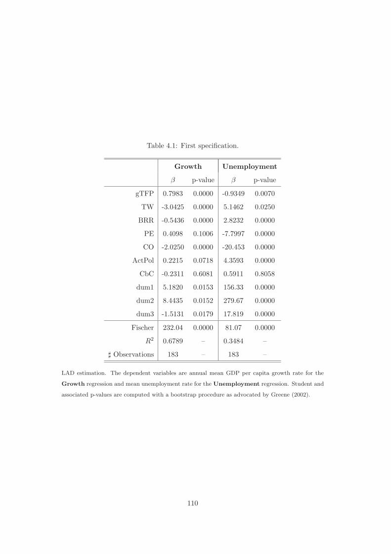
Table 4.1: First specification.
Growth Unemployment
β p-value β p-value
gTFP 0.7983 0.0000 -0.9349 0.0070
TW -3.0425 0.0000 5.1462 0.0250
BRR -0.5436 0.0000 2.8232 0.0000
PE 0.4098 0.1006 -7.7997 0.0000
CO -2.0250 0.0000 -20.453 0.0000
ActPol 0.2215 0.0718 4.3593 0.0000
CbC -0.2311 0.6081 0.5911 0.8058
dum1 5.1820 0.0153 156.33 0.0000
dum2 8.4435 0.0152 279.67 0.0000
dum3 -1.5131 0.0179 17.819 0.0000
Fischer 232.04 0.0000 81.07 0.0000
R2 0.6789 – 0.3484 –
] Observations 183 – 183 –
LAD estimation. The dependent variables are annual mean GDP per capita growth rate for the
Growth regression and mean unemployment rate for the Unemployment regression. Student and
associated p-values are computed with a bootstrap procedure as advocated by Greene (2002).
110
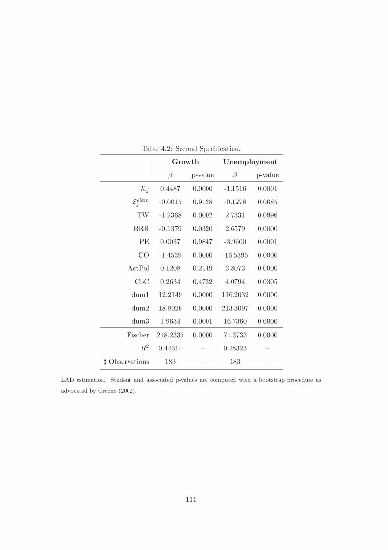
Table 4.2: Second Specification.
Growth Unemployment
β p-value β p-value
Kj 0.4487 0.0000 -1.1516 0.0001
Ee&mj -0.0015 0.9138 -0.1278 0.0685
TW -1.2368 0.0002 2.7331 0.0996
BRR -0.1379 0.0320 2.6579 0.0000
PE 0.0037 0.9847 -3.9600 0.0001
CO -1.4539 0.0000 -16.5395 0.0000
ActPol 0.1208 0.2149 3.8073 0.0000
CbC 0.2634 0.4732 4.0794 0.0305
dum1 12.2149 0.0000 116.2032 0.0000
dum2 18.8026 0.0000 213.3097 0.0000
dum3 1.9634 0.0001 16.7360 0.0000
Fischer 218.2335 0.0000 71.3733 0.0000
R2 0.44314 – 0.28323 –
] Observations 183 – 183 –
LAD estimation. Student and associated p-values are computed with a bootstrap procedure as
advocated by Greene (2002).
111
• The tax wedge (TW) and the unemployment benefits (BRR) lower the growth rates but
increase the unemployment rates,
• The coordination of the wage bargaining (CO) lowers the growth rates and the unemploy-
ment rates.
• Either the growth rate of the regional capital share, or the growth rate of the TFP, increase
(decrease) the GDP per capita growth (the unemployment).
• The bargaining power increases the unemployment in the second specification.
Finally, for the growth and unemployment equations, in the first specification the R2 are respec-
tively 44% and 28%, meaning that our collection of labor market related policy variables and
the growth rate of the two regional-specific variables explains about 1/2 of the heterogeneity of
the growth rates and roughly 1/3 of the heterogeneity of the unemployment rates. Likewise, in
the second specification these values are respectively 68% and 35%, meaning that our collection
of labor market related policy variables and the growth rate of the TFP explains more than
2/3 of the heterogeneity in growth rates and roughly 1/3 of the heterogeneity in unemployment
rates. As expected, the role of Solow residuals is much more important explaining growth than
unemployment.
Counterfactuals
In this section, we propose to evaluate the marginal impact of both national (each labor market
institution) and regional (the growth rate of the TFP) components on the predicted growth and
unemployment rate of an European region.
The methodology
Let considers the following experience. We assume that a Region j′ in France has the same
environment than a region j in UK excepting for one of its national specific variables (labor
market policies) or its specific regional one. Using the estimation of the growth and unemploy-
ment rate, this experience allows us to evaluate the marginal impact of the national/regional
specific variables.
More precisely, we construct these counterfactual experiences as follows:
112
• Predicted GDP per capita growth of Region j in UK is defined by:
gj,UK = cg + XUK βg + SRj,UK βg
with XUK ≡ (TWUK , BRRUK , PEUK , COUK , ActPolUK , CbCUK)
• Suppose that Region j′ in France is as Region j in UK with respect to all the conditioning
variables except Tax Wedge. Hence Region j′ in France counterfactual GDP per capita
growth will be:
gTWj′,FR = cg + X TW
FR βg + SRj′,UK βg
with X TWFR ≡ (TWFR, BRRUK , PEUK , COUK , ActPolUK , CbCUK)
The gap between gj′,FR and gTWj′,FR gives a measure of the marginal effect of the French
fiscal policy.
The results
Due to the high number of Regions (183), we focus only on typical cases. Then, we assume that
the reference is London, and we choose to evaluate the marginal impact of typical European
labor market experience. Then, we choose a north continental country (France), a south conti-
nental country (Spain) and a Nordic country (Sweden). In the two first countries, we propose
to evaluate the marginal impacts of the explanatory variable in two Regions: a Region highly
developed and a poor one. For France, we choose “Ile de France” because this Region encom-
passes Paris, and “Corse”. For Sapin, we choose “Madrid” and “Andalucia”.
Figures 4.6 and 4.7 present the results for the French economy. First in figure 4.6, we show
that the predictions of the econometric model are close to the observed values. The point TW
represents the prediction of the model if all the explanatory variables, except the taxes, are the
same than in London. Hence, the gap between the prediction for London and this point gives
a measure of the marginal impact of the French tax8. The higher unemployment and the lower
growth in Paris than in London are mainly due to the higher tax (TW) and to a lower growth in
TFP (gTFP). Moreover, the wage bargaining coordination (CO) in France leads to less unem-
ployment but at the price of a lower growth rate of the GDP per capita. Second, in figure 4.7,
we show that the predictions of the model are quit poor for Corse, the poorest French Region.8The same is tue for all the explanatory variables: employment protection (PE), unemployment benefits (Brr),
etc...
113
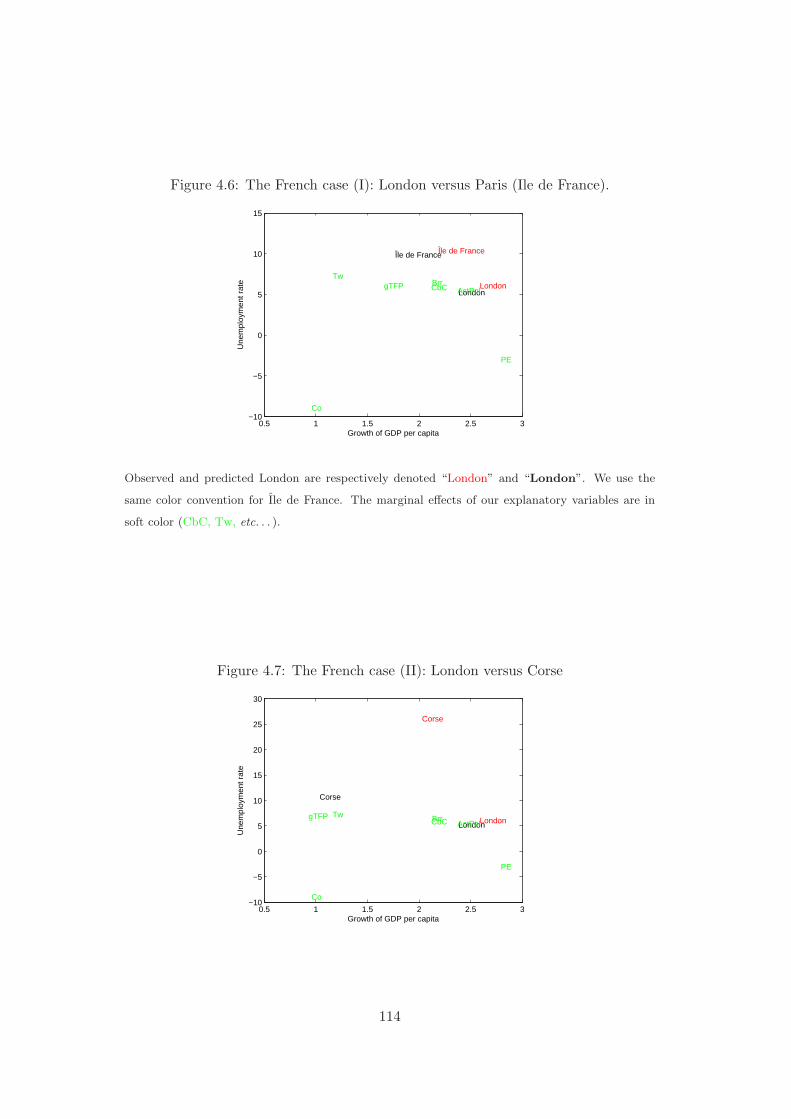
Figure 4.6: The French case (I): London versus Paris (Ile de France).
0.5 1 1.5 2 2.5 3−10
−5
0
5
10
15
London London
gTFPTw
Brr
PE
Co
ActPolCbC
Île de France Île de France
Growth of GDP per capita
Une
mpl
oym
ent r
ate
Observed and predicted London are respectively denoted “London” and “London”. We use the
same color convention for Ile de France. The marginal effects of our explanatory variables are in
soft color (CbC, Tw, etc. . . ).
Figure 4.7: The French case (II): London versus Corse
0.5 1 1.5 2 2.5 3−10
−5
0
5
10
15
20
25
30
London LondongTFP Tw Brr
PE
Co
ActPolCbC
Corse
Corse
Growth of GDP per capita
Une
mpl
oym
ent r
ate
114
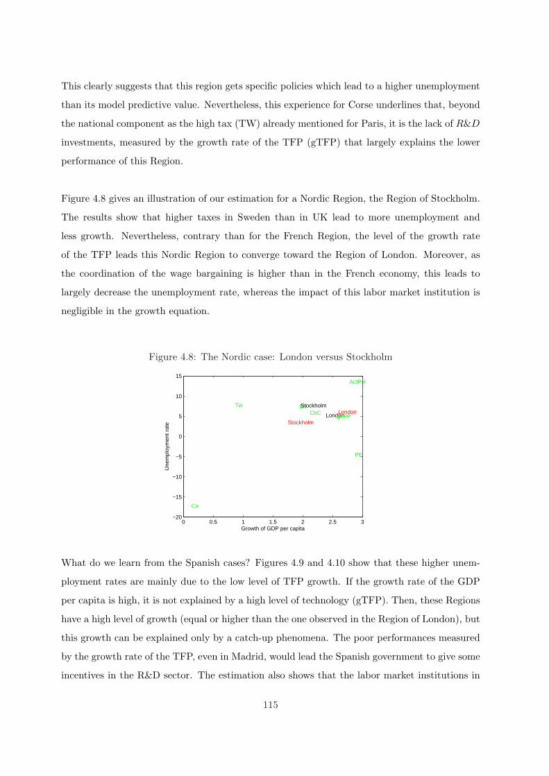
This clearly suggests that this region gets specific policies which lead to a higher unemployment
than its model predictive value. Nevertheless, this experience for Corse underlines that, beyond
the national component as the high tax (TW) already mentioned for Paris, it is the lack of R&D
investments, measured by the growth rate of the TFP (gTFP) that largely explains the lower
performance of this Region.
Figure 4.8 gives an illustration of our estimation for a Nordic Region, the Region of Stockholm.
The results show that higher taxes in Sweden than in UK lead to more unemployment and
less growth. Nevertheless, contrary than for the French Region, the level of the growth rate
of the TFP leads this Nordic Region to converge toward the Region of London. Moreover, as
the coordination of the wage bargaining is higher than in the French economy, this leads to
largely decrease the unemployment rate, whereas the impact of this labor market institution is
negligible in the growth equation.
Figure 4.8: The Nordic case: London versus Stockholm
0 0.5 1 1.5 2 2.5 3−20
−15
−10
−5
0
5
10
15
London LondongTFP
Tw Brr
PE
Co
ActPol
CbC
Stockholm
Stockholm
Growth of GDP per capita
Une
mpl
oym
ent r
ate
What do we learn from the Spanish cases? Figures 4.9 and 4.10 show that these higher unem-
ployment rates are mainly due to the low level of TFP growth. If the growth rate of the GDP
per capita is high, it is not explained by a high level of technology (gTFP). Then, these Regions
have a high level of growth (equal or higher than the one observed in the Region of London), but
this growth can be explained only by a catch-up phenomena. The poor performances measured
by the growth rate of the TFP, even in Madrid, would lead the Spanish government to give some
incentives in the R&D sector. The estimation also shows that the labor market institutions in
115
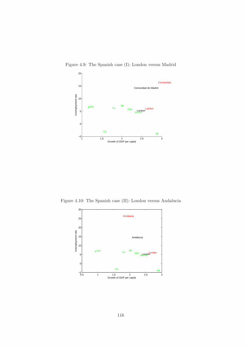
Figure 4.9: The Spanish case (I): London versus Madrid
1 1.5 2 2.5 3−5
0
5
10
15
20
London London
gTFP TwBrr
PECo
ActPolCbC
Comunidad de Madrid
Comunidad de Madrid
Growth of GDP per capita
Une
mpl
oym
ent r
ate
Figure 4.10: The Spanish case (II): London versus Andalucia
0.5 1 1.5 2 2.5 3−5
0
5
10
15
20
25
30
London London
gTFP TwBrr
PECo
ActPolCbC
Andalucia
Andalucia
Growth of GDP per capita
Une
mpl
oym
ent r
ate
116
Spain lead to better economic performances than in France, for exemple.
4.2 The model
At the light of the empirical results, we develop the next theoretical model.
4.2.1 Preferences
The economy is populated by L identical agents, each endowed with one unit flow of labor.
At each time, they may be employed (x), trying their hand at R&D (n) or unemployed (u):
L = x+n+u. When employed, workers pay a tax τw on their labor income. When unemployed,
they receive the unemployment benefits B.
All individuals have the same linear preferences over lifetime consumption of a single final good:
U(Ct) = E0
∫ ∞
0Cte
−ρtdt (4.3)
where ρ > 0 is the subjective rate of time preference and Ct is the per capita consumption
of the final good at time t. Each household is free to borrow and lend at interest rate rt.
However, given linear preferences, the optimal household’s behavior implies ρ = rt ∀t. Hence,
the level of consumption is undefined. A standard solution to this problem is to assume that
households consume all their wage income. This assumption allows us to analyze the impact of
the unemployment benefit system.
4.2.2 Goods sector
The final good is produced by perfectly competitive firms that use the latest vintage of a con-
tinuum of intermediate inputs xj ,
Ct =∫ 1
0Aj,tx
αj,tdj, 0 < α < 1, j ∈ [0, 1] (4.4)
Aj represents the productivity of the intermediate good j and is determined by the number of
technical improvements realized up to date t, knowing that between two consecutive innovations
the gain in productivity is equal to q > 1 (At+1 = qAt).
In turn, intermediate goods are produced by monopolistic firms. Production of one unit of
intermediate good requires one unit of labor as input. Since the final-good sector is perfectly
competitive, the price of each intermediate good, p(xj), is equal to the value of its marginal
117
product:
p(xj,t) =∂C
∂xj,t= αAj,tx
α−1j,t ∀j (4.5)
4.2.3 R&D sector
Technology improvements lead to good-specific public knowledge allowing to start improvement
efforts upon the current vintage v. Innovations on good j arrive randomly at a Poisson rate
hnj , where nj is the amount of labor used in R&D, and h > 0 a parameter indicating the
productivity of the research technology. Finally, the size of the R&D sector is given by the
arbitrage condition:9
(1− τw)Wj′,v
h≤ min
jVj,v+1 ∀j, j′ ∈ [0, 1] (4.6)
That is, the opportunity cost of R&D is the hourly net wage prevailing in the production sector,
industry j, (1− τw)Wj′,v, times the expected duration of the innovation process, 1/h.10 On the
other hand, the expected payoff of next innovation, Vj,v+1, is equal to the net discounted value
of an asset yielding Πj,v+1 per period until the arrival of next innovation, at the arrival rate
hnj,v+1.
We assume that the employment protection laws imply a cost E of shutting down a firm, which
occurs as current producers are replaced by next ones. Then:
Vj,v+1 =Πj,v+1 − hnj,v+1Ev+1
r + hnj,v+1(4.7)
Assuming that Firms pay a proportional payroll tax τ over employment, the instantaneous
monopolistic profits earned by the successful innovator are:
Πj,v+1 = p(xj,v+1)xj,v+1 −Wj,v+1(1 + τ)xj,v+1 (4.8)
Normalizing the lasts expressions by the productivity level associated to the (v+1)th innovation,
and using equation (4.5) we obtain:
πj,v+1 = αxαj,v+1 − wj(1 + τ)xj,v+1 (4.9)
9Equivalently, the entry condition also reflects the fact that labor can be freely allocated between production
and research: (1 − τw)Wj′,v is the net value of an hour in production while hVj,v+1 is the expected value of an
hour in research.10Equivalently, we can assume that the opportunity cost amounts to the unemployment benefits, or even to a
linear combination of both, the earnings of employed and those of unemployed workers.
118
hence the free entry (D.3) condition becomes:
(1− τw)wj′,v ≤ qhνj,v+1 (4.10)
= qh
(πj,v+1 − hnj,v+1e
r + hnj,v+1
)
for π ≡ ΠA , w ≡ W
A , e ≡ EA and ν ≡ V
A .
4.2.4 Government
The government faces the following budget constraint:
Bu + T = (τ + τw)∫ 1
0wjxjdj + Eh
∫ 1
0njdj (4.11)
Any change in the revenue caused by changes in taxes and subsidies is rebated to household
through the lump-sum transfer T .
4.2.5 Wage bargaining and labor demand
The wage rate is the solution to the bargaining problem between the monopolistic producer of
good j and the trade union representing the workers’ interests. We model the bargaining process
as a a generalized Nash bargaining game, with union’s relative bargaining power β. If they don’t
agree, workers get the unemployment benefits and the monopolist pays the firing costs E. Given
the bargained wages, the firm chooses the level of employment that maximizes her profit flow.
That is,
Wj,v+1 = arg max
[((1−τw)Wj,v+1−Bj,v+1)x(Wj,v+1)]β(Πj,v+1−hnj,v+1E−πj,v+1)1−β
(4.12)
πj,v+1 ≡ −hnj,v+1E denotes the firm’s disagreement point.
4.2.6 Equilibrium
Given ρ > 0, for all intermediate good sector j and for all vintage v a steady-state (or balanced
growth path) equilibrium is defined as follows:
(i) Wage rule:
w =β1b
1− t, β1 ≡ 1 +
β(1− α)α
(4.13)
for w ≡ WA
119
(ii) Labor demand:
x =(
α2(1− τw)(1 + τ)β1b
) 11−α
(4.14)
(iii) R&D
The symmetry on wages and so on labor demand imply that the expected gains from
an innovation are identical across industries: Vj′ = Vj ∀j, j′ ∈ [0, 1]. By consequence the
amount of labor allocated to R&D is the same for any intermediate good j: nj = n. Hence,
from the free entry condition we deduce:
n =(
1h
)(qhπ − rβ1b
β1b + qhe
)(4.15)
where
π =(1− α)(1 + τ)β1b
α(1− τw)x (4.16)
(iv) Unemployment:
Unemployment u is deduced from the employment identity given the endowment of labor
L, the labor demand for production x and the aggregate number of potential innovators
n:
u = L− x− n (4.17)
(v) Government:
The balanced budget of government is:
bu +> = (τ + τw)wx + ehn (4.18)
were b ≡ BA , and > ≡ T
A .
(vi) Economic growth: Between two consecutive innovations final output is augmented a
fixed amount q: Cv+1 = qCv. Then, between date t and date t + 1 expected output is:
E[Ct+1] = q∫ 10 hntdtCt
By taking logarithms and arranging terms we get:
gt ≡ E[lnCt+1 − lnCt] = hnt ln(q)
Then, at the steady state (nt = n):
g = hn ln(q) (4.19)
120
4.3 The impact of labor market institutions on growth and un-
employment
4.3.1 Labor market policies
In this section we analyze the consequences for growth and unemployment of, (ii) a more gen-
erous unemployment insurance, (ii) higher taxes on labor incomes, and (iii) the employment
protection.
Proposition. 1 An increase in the unemployment compensation (b), or in the payroll taxes (τ),
or in the taxes on labor income (τw) or in the employment protection (e), leads to (i) higher
unemployment and (ii) lower rate of growth.
This result is very intuitive (see the proof in the appendix): higher labor costs imply higher
wages (equation (4.13)) and so a decline in the labor demand (equation (4.14)). This contracts
the monopolistic profits and reduces the expected value of an innovation. Moreover, the higher
wages make production more attractive than R&D. As the size of R&D decline, the growth rate
falls. Since neither the wage rates nor the labor demands change, the only effect is a contraction
of profits. This reduces the workers’ incentives to engage in R&D. Then the growth rate falls
and the unemployment raises.
4.3.2 The wage bargaining processes
The impact of unions is analyzed in two steps. First, for an uncoordinated wage bargaining
process we derive the implications of a higher bargaining power. Second, we can compare the
outcome of an efficient bargaining process (that is, with simultaneous bargain of wages and labor
demand) with the inefficient outcome computed above.
The bargaining power
Proposition. 2 An increase in the unions’ bargaining power leads to an increase in the unem-
ployment level and to a decrease in the economic growth.
The economic intuition is the following (see the proof in the appendix): a bigger bargaining
power implies higher wages. Then the labor demand for production declines, this contracts the
monopolistic profits and so the expected value of an innovation. This discourages workers from
R&D. The total outcome is higher unemployment and lower economic growth.
121
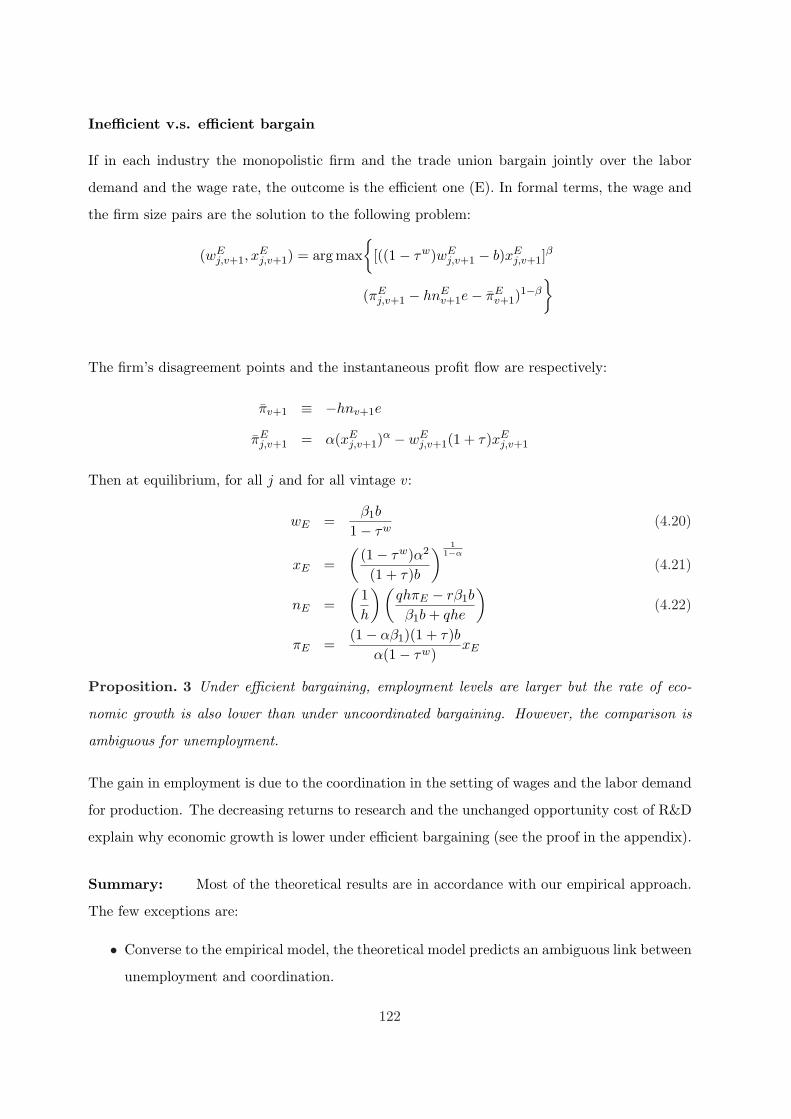
Inefficient v.s. efficient bargain
If in each industry the monopolistic firm and the trade union bargain jointly over the labor
demand and the wage rate, the outcome is the efficient one (E). In formal terms, the wage and
the firm size pairs are the solution to the following problem:
(wEj,v+1, x
Ej,v+1) = arg max
[((1− τw)wE
j,v+1 − b)xEj,v+1]
β
(πEj,v+1 − hnE
v+1e− πEv+1)
1−β
The firm’s disagreement points and the instantaneous profit flow are respectively:
πv+1 ≡ −hnv+1e
πEj,v+1 = α(xE
j,v+1)α − wE
j,v+1(1 + τ)xEj,v+1
Then at equilibrium, for all j and for all vintage v:
wE =β1b
1− τw(4.20)
xE =(
(1− τw)α2
(1 + τ)b
) 11−α
(4.21)
nE =(
1h
)(qhπE − rβ1b
β1b + qhe
)(4.22)
πE =(1− αβ1)(1 + τ)b
α(1− τw)xE
Proposition. 3 Under efficient bargaining, employment levels are larger but the rate of eco-
nomic growth is also lower than under uncoordinated bargaining. However, the comparison is
ambiguous for unemployment.
The gain in employment is due to the coordination in the setting of wages and the labor demand
for production. The decreasing returns to research and the unchanged opportunity cost of R&D
explain why economic growth is lower under efficient bargaining (see the proof in the appendix).
Summary: Most of the theoretical results are in accordance with our empirical approach.
The few exceptions are:
• Converse to the empirical model, the theoretical model predicts an ambiguous link between
unemployment and coordination.
122
• Even if the link between the bargaining power and the GDP growth is not significant,
it has the unambiguous sign predicted by our theoretical model. These results can be
explained by the poor approximation of our statistical measure (collective bargaining cov-
erage (CbC)) to the workers’ bargaining power.
4.4 Conclusion
We have constructed a general equilibrium model in which economic growth and unemployment
are endogenously determined by the number of innovations made in the economy, which in turn
is determined by the workers’ incentive to engage in R&D activities. We have shown that high
labor costs or powerful trade unions lead to bigger unemployment and to a slowdown of the
economic growth whereas an efficient bargain allows to higher employment, at the price of a
lower growth rate.
Using a cross-section of European regions and a large set of labor market variables, we find that
national institutions on the labor market are highly correlated with unemployment. Hence, the
tax wedge and the unemployment benefits increase the regional unemployment rates whereas
the employment protection and a high level of coordination in the wage bargaining process
decrease the regional unemployment rates. On the other hand, we find that increases in the
tax wedge and in the unemployment benefits decrease the regional growth rate of GDP per
capita. Nevertheless, a high level of coordination in the wage bargaining process decreases the
regional growth rate of GDP per capita. This last result shows that there is an arbitration
between unemployment and growth if we focuss on the impact of the coordination in the wage
bargaining process. Finally, the empirical results concerning the active labor market policies
(ActPol) suggest to include them into the theoretical model because they have positive impact
on the unemployment rate.
123

Chapter 5
Explaining the evolution of hours
worked and employment across
OECD countries: an equilibrium
search approach
This chapter is based on a joint paper with Francois Langot (IZA DP No. 3364, February 2008)
124
Introduction
Aggregate hours of market work exhibit dramatic differences across industrialized countries.
What accounts for these differences? In the current literature, there are two candidate ap-
proaches allowing to explain these differences.
A first set of contributions focus on the decline of the average hours worked per employee (the
intensive margin) in European countries since 1960. Prescott (2004) studies the role of taxes
in accounting for differences in labor supply across time and across countries. He finds that
the effective marginal tax rate on labor income explains most of the differences at points of
time and the large change in relative (to US) labor supply over time. On this line of research,
Rogerson (2006) shows that the aggregate hours worked in Continental European countries such
as Belgium, France, Germany and Italy are roughly one third less than in the US. This fact
results from a diverging process in the hours worked per employee in each zone: between 1960
and 1980, whereas in Europe we observe a large decrease, in the US this decline is very small;
and after 1980, we observe in the two zones a stable number of hours worked per employee. This
evolution of the hours worked per employee is strongly correlated to the dynamics of the taxes.
Hence, as it is suggested by Prescott (2004), Rogerson (2006) or Ohanian, Raffo, and Rogerson
(2006), a theory providing a link between the hours worked per employee and taxes seems to be
sufficient to explain why Europeans work less than Americans.
However, since 1980 a notable feature of the data is that differences across countries in aggregate
hours are due to quantitatively important differences along the extensive margin. Hence, a
second set of contributions (see e.g. Jackman, Layard, and Nickell (1991), Mortensen and
Pissarides (1999a), Blanchard and Wolfers (2000) or Ljungqvist and Sargent (2007b)) considers
that the large decrease of the employment rate observed after 1980 in the European countries, is
an important factor of the dynamics of total hours. These works show that different labor market
institutions lead to different labor market outcomes after a common shock. In these previous
papers, there is fairly robust evidence that (i) the level and duration of unemployment benefits
and (ii) the union’s bargaining power have a significant positive impact on unemployment1
To sum up, the main factors explaining the decline in the hours worked per employee differ from1There is less consensus on the effects of the employment protection legislation. At the opposite, there is
some labor market institutions associated with lower unemployment: highly centralized and/or coordinated wage
bargaining systems, as well as some categories of public spending on active labor market programmes. See Daveri
and Tabellini (2000) or Bassanini and Duval (2006) who provide a review of recent literature on this topic.
125
those explaining the decline in the employment rate: the taxes for the former, and the labor
market institutions, such as the unions’ power or the unemployment benefits, for the second.
Clearly, all together contribute to the dynamics of the two margins of the total hours.
From a theoretical point of view, the aim of this chapter is to provide a theory allowing to account
for the impact, of both taxes and labor market institutions, on the two margins of the aggregate
hours worked. To this end, we follow the empirical methodology presented in Ohanian, Raffo,
and Rogerson (2006): the quantitative evaluation of the model and the impact of distortions
is based on the computation of series for the gap between the marginal cost and the marginal
return of labor that is produced using actual data and model restrictions2. Furthermore, we
extend the theoretical investigation: beyond the usual neo-classical growth model which allows
to predict the hours worked per employee, we explore the ability of the Hansen (1985)-Rogerson
(1988) model to reproduce the dynamics of the employment rate. Finally, we develop a general
equilibrium matching model, close to the one proposed by Andolfatto (1996), Feve and Langot
(1996) and Cheron and Langot (2004), allowing to explain the dynamics of both the hours
worked per employee and the employment rate. This last model is rich enough to allow the
evaluation of the relative contribution of the tax/benefit systems and unions in the explanation
of the observed allocation of time.
Our sample consists of six countries: Belgium, Spain, France, Italy, United Kingdom and the
United States. Depending on the availability of data, the analysis covers the 1980-2003 or the
1960-2003 period. The main findings are the following. First, the long-run decline in the hours
worked per employee is mainly due to the increase of the taxes, as it is suggested by Prescott
(2004), Rogerson (2006) and Ohanian, Raffo, and Rogerson (2006). Second, the employment
rate is affected by institutional aspects of the labor market, such as the bargaining power and the
unemployment benefits, rather than by taxes, conversely to the individual work effort. Finally,
this behavior of the two margins of the aggregate hours is well accounted by our search model,
when it includes the observed heterogeneity of the tax/benefit systems and the labor market
indicators of the wage-setting process across countries. These findings give some support to the
two explanations of the European decline in total hours: the important role of taxes through
the intensive margin and the large contribution of the labor market institutions through the
extensive margin. Because these findings come from an unified framework, they also give a
strong support to the matching models.2The closer these gaps are to zero, the better the model accounts for the observed labor behavior.
126
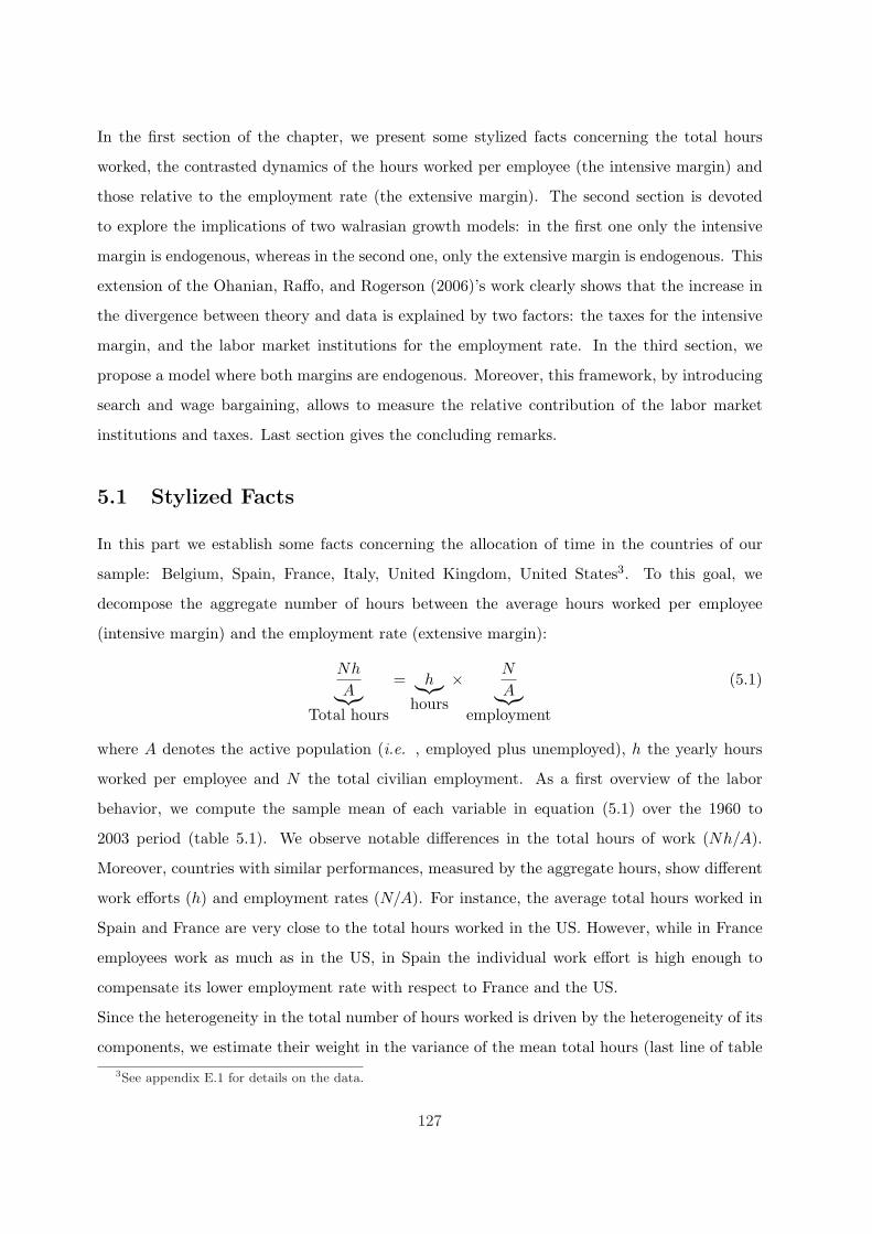
In the first section of the chapter, we present some stylized facts concerning the total hours
worked, the contrasted dynamics of the hours worked per employee (the intensive margin) and
those relative to the employment rate (the extensive margin). The second section is devoted
to explore the implications of two walrasian growth models: in the first one only the intensive
margin is endogenous, whereas in the second one, only the extensive margin is endogenous. This
extension of the Ohanian, Raffo, and Rogerson (2006)’s work clearly shows that the increase in
the divergence between theory and data is explained by two factors: the taxes for the intensive
margin, and the labor market institutions for the employment rate. In the third section, we
propose a model where both margins are endogenous. Moreover, this framework, by introducing
search and wage bargaining, allows to measure the relative contribution of the labor market
institutions and taxes. Last section gives the concluding remarks.
5.1 Stylized Facts
In this part we establish some facts concerning the allocation of time in the countries of our
sample: Belgium, Spain, France, Italy, United Kingdom, United States3. To this goal, we
decompose the aggregate number of hours between the average hours worked per employee
(intensive margin) and the employment rate (extensive margin):
Nh
A︸︷︷︸Total hours
= h︸︷︷︸hours
× N
A︸︷︷︸employment
(5.1)
where A denotes the active population (i.e. , employed plus unemployed), h the yearly hours
worked per employee and N the total civilian employment. As a first overview of the labor
behavior, we compute the sample mean of each variable in equation (5.1) over the 1960 to
2003 period (table 5.1). We observe notable differences in the total hours of work (Nh/A).
Moreover, countries with similar performances, measured by the aggregate hours, show different
work efforts (h) and employment rates (N/A). For instance, the average total hours worked in
Spain and France are very close to the total hours worked in the US. However, while in France
employees work as much as in the US, in Spain the individual work effort is high enough to
compensate its lower employment rate with respect to France and the US.
Since the heterogeneity in the total number of hours worked is driven by the heterogeneity of its
components, we estimate their weight in the variance of the mean total hours (last line of table3See appendix E.1 for details on the data.
127
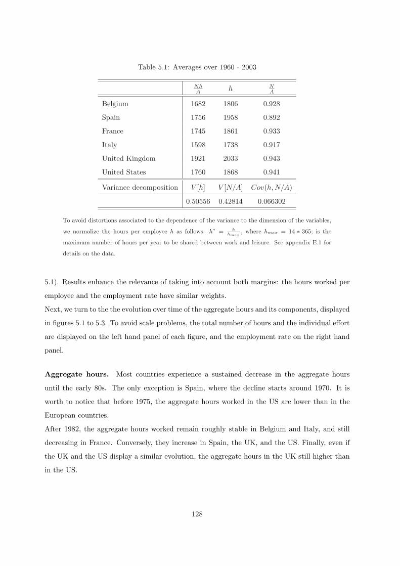
Table 5.1: Averages over 1960 - 2003
NhA h N
A
Belgium 1682 1806 0.928
Spain 1756 1958 0.892
France 1745 1861 0.933
Italy 1598 1738 0.917
United Kingdom 1921 2033 0.943
United States 1760 1868 0.941
Variance decomposition V [h] V [N/A] Cov(h, N/A)
0.50556 0.42814 0.066302
To avoid distortions associated to the dependence of the variance to the dimension of the variables,
we normalize the hours per employee h as follows: h∗ = hhmax
, where hmax = 14 ∗ 365; is the
maximum number of hours per year to be shared between work and leisure. See appendix E.1 for
details on the data.
5.1). Results enhance the relevance of taking into account both margins: the hours worked per
employee and the employment rate have similar weights.
Next, we turn to the the evolution over time of the aggregate hours and its components, displayed
in figures 5.1 to 5.3. To avoid scale problems, the total number of hours and the individual effort
are displayed on the left hand panel of each figure, and the employment rate on the right hand
panel.
Aggregate hours. Most countries experience a sustained decrease in the aggregate hours
until the early 80s. The only exception is Spain, where the decline starts around 1970. It is
worth to notice that before 1975, the aggregate hours worked in the US are lower than in the
European countries.
After 1982, the aggregate hours worked remain roughly stable in Belgium and Italy, and still
decreasing in France. Conversely, they increase in Spain, the UK, and the US. Finally, even if
the UK and the US display a similar evolution, the aggregate hours in the UK still higher than
in the US.
128
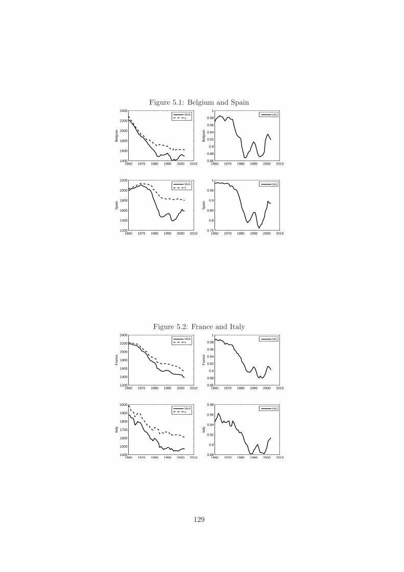
Figure 5.1: Belgium and Spain
1960 1970 1980 1990 2000 20101400
1600
1800
2000
2200
2400
Bel
gium
Nh/Ah
1960 1970 1980 1990 2000 20100.86
0.88
0.9
0.92
0.94
0.96
0.98
1
Bel
gium
N/A
1960 1970 1980 1990 2000 20101200
1400
1600
1800
2000
2200
Spa
in
Nh/Ah
1960 1970 1980 1990 2000 20100.75
0.8
0.85
0.9
0.95
1
Spa
in
N/A
Figure 5.2: France and Italy
1960 1970 1980 1990 2000 20101200
1400
1600
1800
2000
2200
2400
Fra
nce
Nh/Ah
1960 1970 1980 1990 2000 20100.86
0.88
0.9
0.92
0.94
0.96
0.98
1
Fra
nce
N/A
1960 1970 1980 1990 2000 20101400
1500
1600
1700
1800
1900
2000
Italy
Nh/Ah
1960 1970 1980 1990 2000 20100.88
0.9
0.92
0.94
0.96
0.98
Italy
N/A
129
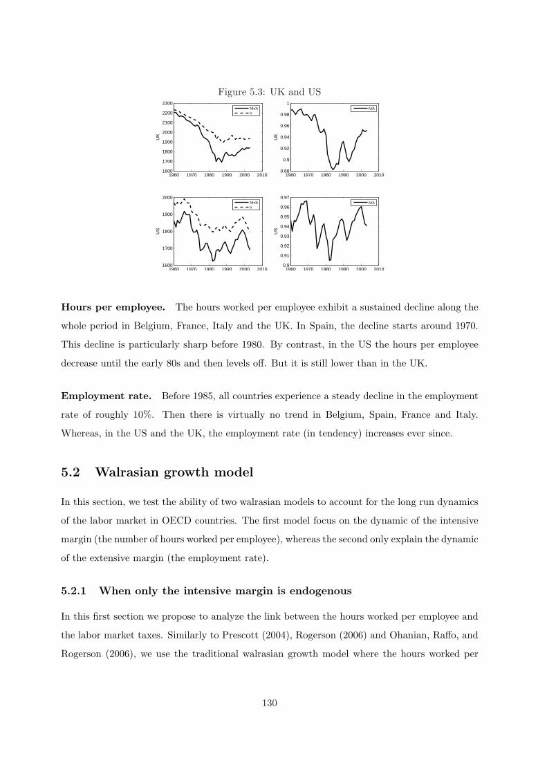
Figure 5.3: UK and US
1960 1970 1980 1990 2000 20101600
1700
1800
1900
2000
2100
2200
2300
UK
Nh/Ah
1960 1970 1980 1990 2000 20100.88
0.9
0.92
0.94
0.96
0.98
1
UK
N/A
1960 1970 1980 1990 2000 20101600
1700
1800
1900
2000
US
Nh/Ah
1960 1970 1980 1990 2000 20100.9
0.91
0.92
0.93
0.94
0.95
0.96
0.97
US
N/A
Hours per employee. The hours worked per employee exhibit a sustained decline along the
whole period in Belgium, France, Italy and the UK. In Spain, the decline starts around 1970.
This decline is particularly sharp before 1980. By contrast, in the US the hours per employee
decrease until the early 80s and then levels off. But it is still lower than in the UK.
Employment rate. Before 1985, all countries experience a steady decline in the employment
rate of roughly 10%. Then there is virtually no trend in Belgium, Spain, France and Italy.
Whereas, in the US and the UK, the employment rate (in tendency) increases ever since.
5.2 Walrasian growth model
In this section, we test the ability of two walrasian models to account for the long run dynamics
of the labor market in OECD countries. The first model focus on the dynamic of the intensive
margin (the number of hours worked per employee), whereas the second only explain the dynamic
of the extensive margin (the employment rate).
5.2.1 When only the intensive margin is endogenous
In this first section we propose to analyze the link between the hours worked per employee and
the labor market taxes. Similarly to Prescott (2004), Rogerson (2006) and Ohanian, Raffo, and
Rogerson (2006), we use the traditional walrasian growth model where the hours worked per
130
employee are divisible: full-employment insures that the employment rate is constat and that
all the labor market adjustments are driven by the intensive margin.
Behaviors
The economy is populated by a large number of identical households whose measure is normalized
to one. Each household consists of a continuum of infinitely-lived agents. At each period there
is full employment: Nt = 1, ∀t. The representative household’s preferences are
∞∑
t=0
βtU(Ct, 1− ht) (5.2)
where 0 < β < 1 is the discount factor. Ct stands for per capita consumption and 1− ht for the
leisure time. The contemporaneous utility function is assumed to be increasing and concave in
both arguments and it shows conventional separability between consumption and leisure:
U(Ct, 1− ht) = lnCt + σ ln(1− ht) σ > 0
The capital stock Kt is rented to firms at net price (rt + δ), where 0 < δ < 1 is the depreciation
rate of capital. Each household chooses Ct, ht,Kt+1|t ≥ 0 to maximize (5.2) subject to the
budget constraint
(1 + Rt)Kt + (1− τw,t)wtht + Lt + πt −Kt+1 − (1 + τc,t)Ct ≥ 0 (λt) (5.3)
where Rt = (1 − τk)r is the effective interest rate, τk is the capital income tax rate, τc is the
consumption tax rate, τw the labor income tax rate, and b are the unemployment benefits. L
is a lump-sum transfer from the government. We assume a balanced budget at each period. w
and π are the real wage and lump-sum dividends remitted by firms.
Each firm has access to the Cobb-Douglas production technology to produce output. Each
producer maximizes the following profit flow:
πt = AtKαt (ht)1−α − (1 + τf,t)wtht − (rt + δ)Kt (5.4)
where 0 < α < 1 and τf stands for the payroll taxes. Then, we have maxπ = 0.
131
The equilibrium and parameterization
Let λt be the shadow price of the budget constraint, the optimality conditions of these problems
lead to:
λt = ((1 + τc,t)Ct)−1 (5.5)
wt =σ(1− ht)−1
(1− τw,t)λt(5.6)
1 = β
[λt+1
λt
(1 + (1− τk,t+1)
(α
Yt+1
Kt+1− δ
))](5.7)
wt =(1− α)Yt
(1 + τf,t)ht(5.8)
Therefore, the labor market equilibrium is then determined by:
(1− α)Yt
ht=
(1 + τf,t)(1 + τc,t)
1− τw,t
σ(1− ht)−1Ct (5.9)
⇔ MPHwt = (1 + TWt)×MRS(H/C)t
where MPHwt and MRS(H/C) denote respectively the marginal product of an hour worked
and the marginal rate of substitution between hours worked and consumption. The tax wedge
is defined by:
1 + TWt =(1 + τf,t)(1 + τc,t)
1− τw,t
Following Ohanian, Raffo, and Rogerson (2006), one can compute the gap between the return
and the cost of the marginal hours worked as follows:
MRS(H/C)t = (1−∆h,wt )MPHw
t for TW = 0 ⇒ ∆h,wt = 1− MRS(H/C)t
MPHwt
In this case, the measure of ∆h,wt includes the restriction of full employment (Nt = 1). Hence,
Yt is measured by the aggregate production per capita, Ct by the aggregate consumption per
capita and ht by the average number of hours worked per employee. Finally, in order to compute
the empirical counterpart of ∆h,wt , we choose the same parameters of the structural model than
in Ohanian, Raffo, and Rogerson (2006): α = .4 and σ = 2.
If the labor supply is evaluated without the tax wedge, i.e. if TW = 0, we have, under the
assumption that the model is able to generate the observed data MPHwt > MRS(H/C)t. From
the point of view of the econometrician, for a given known set of structural parameters, ∆h,wt is
the residual of the the first order equation estimated with an omitted variable, the tax wedge. If
this omitted variable has a trend component, the estimation of ∆h,wt has also this trend. Hence,
132
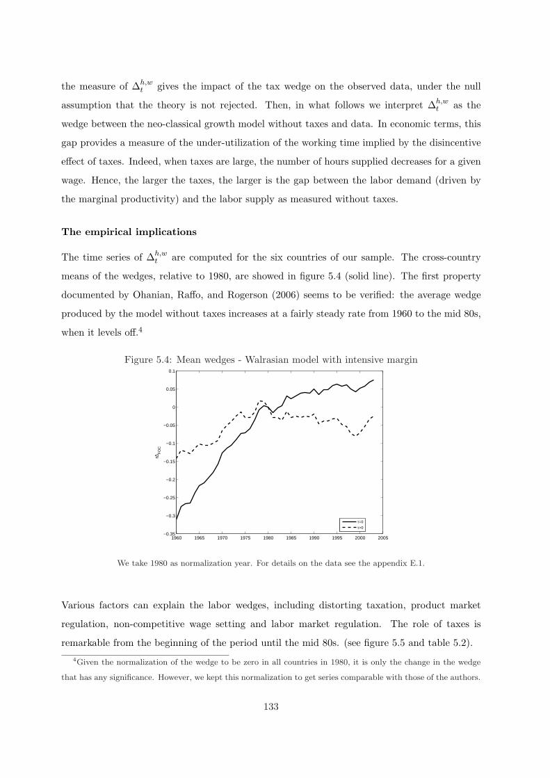
the measure of ∆h,wt gives the impact of the tax wedge on the observed data, under the null
assumption that the theory is not rejected. Then, in what follows we interpret ∆h,wt as the
wedge between the neo-classical growth model without taxes and data. In economic terms, this
gap provides a measure of the under-utilization of the working time implied by the disincentive
effect of taxes. Indeed, when taxes are large, the number of hours supplied decreases for a given
wage. Hence, the larger the taxes, the larger is the gap between the labor demand (driven by
the marginal productivity) and the labor supply as measured without taxes.
The empirical implications
The time series of ∆h,wt are computed for the six countries of our sample. The cross-country
means of the wedges, relative to 1980, are showed in figure 5.4 (solid line). The first property
documented by Ohanian, Raffo, and Rogerson (2006) seems to be verified: the average wedge
produced by the model without taxes increases at a fairly steady rate from 1960 to the mid 80s,
when it levels off.4
Figure 5.4: Mean wedges - Walrasian model with intensive margin
1960 1965 1970 1975 1980 1985 1990 1995 2000 2005−0.35
−0.3
−0.25
−0.2
−0.15
−0.1
−0.05
0
0.05
0.1
r∆F
OC
τ=0
τ>0
We take 1980 as normalization year. For details on the data see the appendix E.1.
Various factors can explain the labor wedges, including distorting taxation, product market
regulation, non-competitive wage setting and labor market regulation. The role of taxes is
remarkable from the beginning of the period until the mid 80s. (see figure 5.5 and table 5.2).4Given the normalization of the wedge to be zero in all countries in 1980, it is only the change in the wedge
that has any significance. However, we kept this normalization to get series comparable with those of the authors.
133
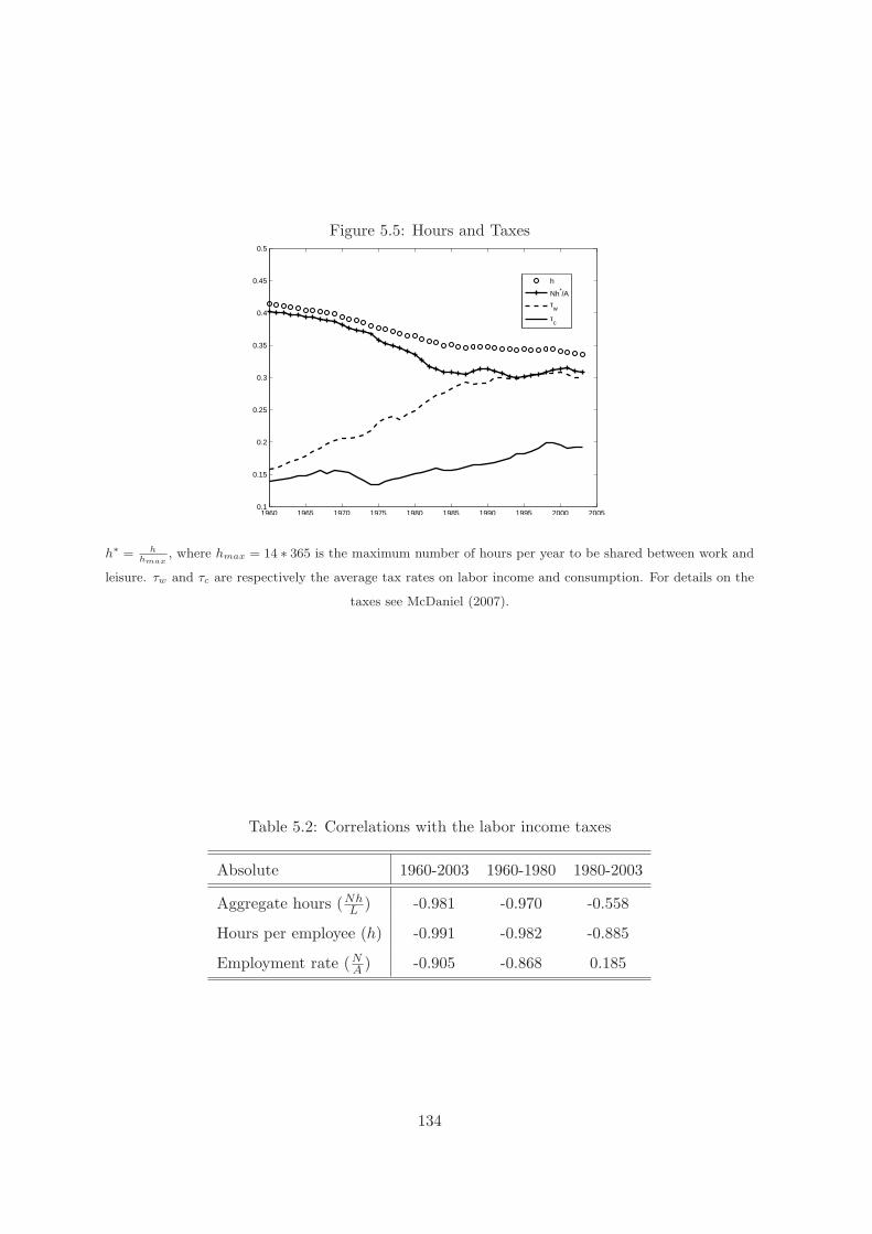
Figure 5.5: Hours and Taxes
1960 1965 1970 1975 1980 1985 1990 1995 2000 20050.1
0.15
0.2
0.25
0.3
0.35
0.4
0.45
0.5
h
Nh*/A
τw
τc
h∗ = hhmax
, where hmax = 14 ∗ 365 is the maximum number of hours per year to be shared between work and
leisure. τw and τc are respectively the average tax rates on labor income and consumption. For details on the
taxes see McDaniel (2007).
Table 5.2: Correlations with the labor income taxes
Absolute 1960-2003 1960-1980 1980-2003
Aggregate hours (NhL ) -0.981 -0.970 -0.558
Hours per employee (h) -0.991 -0.982 -0.885
Employment rate (NA ) -0.905 -0.868 0.185
134
Then, one may expect that the incorporation of distorting taxation reduces the size of the wedge
over time and across the countries. With taxes, the wedges are computed as follows:
(1+TWt)MRS(H/C)t = (1−∆h,wt )MPHw
t for TW > 0 ⇒ ∆h,wt,TW>0 = 1−(1+TWt)
MRS(H/C)t
MPHwt
The dotted line in figure 5.4 confirms our intuition: the size of the gap is reduced over time and
across countries when we consider distorting taxation.
On the other side, the negative impact of the labor market institutions on the performance of
European labor markets after 1980 is well documented. In coherence with the search model
developed in section 5.3, we conduct a simple statistical analysis to assess the impact of two
institutional factors other than taxes that are typically thought to influence the labor market
equilibrium. The strategy is to perform a panel regression to investigate the importance of taxes,
the worker’s bargaining power, and the average replacement rate in explaining the evolution in
wedges. The specification is:
ln(1−∆h,wi,t,TW=0) = ai + b ln(TWi,t − 1) + γBargi,t + βARRi,t + εi,t
where ai is a country-specific fix effect, Bargi,t is the workers’ bargaining power, measured as
the average of the union coverage and the union density (see section 5.3.2), and ARRi,t is the
average replacement rate. The results from the regression (table 5.3) show that taxes have a
significant negative impact on the variation in the hours wedge. This result seems to be robust:
for all the specifications (regressions (1) to (4)), the tax wedge has a negative significant impact
at 5% level. At the opposite, the labor market institutions (LMI) have not significant impact
on this wedge between theory and data. Regression (5) shows that the bargaining power, as the
sole explanatory variable, has not significant effect. Finally, regressions (6) and (7) show that
the average replacement ratio is correlated with taxes: in countries where taxes are high and
follow an increasing path, the unemployment benefit follows this trend. Hence, if we omit taxes
as an explanatory variable, the average replacement ratio has a significant negative impact on
the dynamics of wedge between theory and data. These results give some support to the view
that the increase in taxation is the main explanative factor of the large decrease in the hours
worked in the OECD countries.
To sum up, the average hours per employee decrease since 1960. Without taxation, the wedge
between the first order condition (equation (5.10)) and the data increases over time. Before the
80’s, this negative correlation between the increasing taxes and the hours per employee is large
and then explains the large increase in the wedge ∆h,w. After the 80’s, our empirical results
135
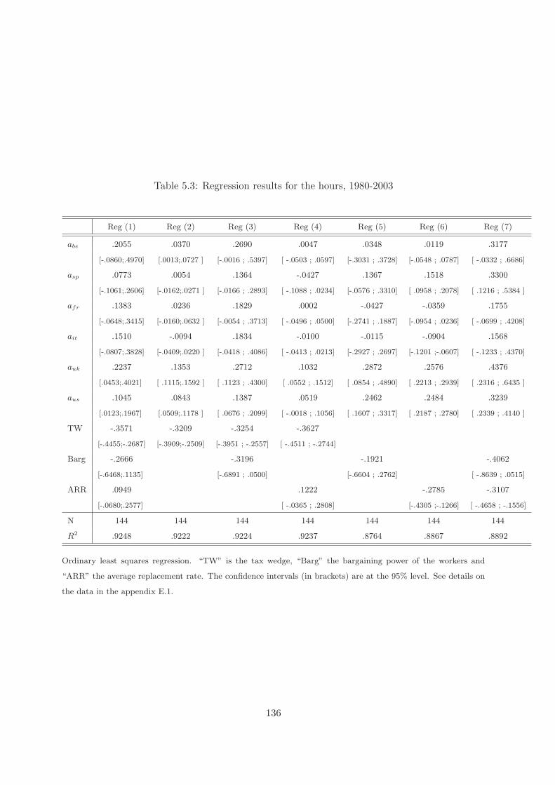
Table 5.3: Regression results for the hours, 1980-2003
Reg (1) Reg (2) Reg (3) Reg (4) Reg (5) Reg (6) Reg (7)
abe .2055 .0370 .2690 .0047 .0348 .0119 .3177
[-.0860;.4970] [.0013;.0727 ] [-.0016 ; .5397] [ -.0503 ; .0597] [-.3031 ; .3728] [-.0548 ; .0787] [ -.0332 ; .6686]
asp .0773 .0054 .1364 -.0427 .1367 .1518 .3300
[-.1061;.2606] [-.0162;.0271 ] [-.0166 ; .2893] [ -.1088 ; .0234] [-.0576 ; .3310] [ .0958 ; .2078] [ .1216 ; .5384 ]
afr .1383 .0236 .1829 .0002 -.0427 -.0359 .1755
[-.0648;.3415] [-.0160;.0632 ] [-.0054 ; .3713] [ -.0496 ; .0500] [-.2741 ; .1887] [-.0954 ; .0236] [ -.0699 ; .4208]
ait .1510 -.0094 .1834 -.0100 -.0115 -.0904 .1568
[-.0807;.3828] [-.0409;.0220 ] [-.0418 ; .4086] [ -.0413 ; .0213] [-.2927 ; .2697] [-.1201 ;-.0607] [ -.1233 ; .4370]
auk .2237 .1353 .2712 .1032 .2872 .2576 .4376
[.0453;.4021] [ .1115;.1592 ] [ .1123 ; .4300] [ .0552 ; .1512] [ .0854 ; .4890] [ .2213 ; .2939] [ .2316 ; .6435 ]
aus .1045 .0843 .1387 .0519 .2462 .2484 .3239
[.0123;.1967] [.0509;.1178 ] [ .0676 ; .2099] [ -.0018 ; .1056] [ .1607 ; .3317] [ .2187 ; .2780] [ .2339 ; .4140 ]
TW -.3571 -.3209 -.3254 -.3627
[-.4455;-.2687] [-.3909;-.2509] [-.3951 ; -.2557] [ -.4511 ; -.2744]
Barg -.2666 -.3196 -.1921 -.4062
[-.6468;.1135] [-.6891 ; .0500] [-.6604 ; .2762] [ -.8639 ; .0515]
ARR .0949 .1222 -.2785 -.3107
[-.0680;.2577] [ -.0365 ; .2808] [-.4305 ;-.1266] [ -.4658 ; -.1556]
N 144 144 144 144 144 144 144
R2 .9248 .9222 .9224 .9237 .8764 .8867 .8892
Ordinary least squares regression. “TW” is the tax wedge, “Barg” the bargaining power of the workers and
“ARR” the average replacement rate. The confidence intervals (in brackets) are at the 95% level. See details on
the data in the appendix E.1.
136

suggest that the dynamics of taxes is still correlated with ∆h,w, whereas it is not correlated
with the LMI. Then the long-run decline in the hours worked per employee is mainly due to the
increase in the taxes as it is suggested by Prescott (2004), Rogerson (2006) and Ohanian, Raffo,
and Rogerson (2006).
5.2.2 When only the extensive margin is endogenous
Given that the employment rate and the average hours worked per employee follow different
paths in some countries, it is interesting to explore the explanative role of taxation along the
extensive margin. To this end, we compute an employment wedge to the equilibrium condition
from the Hansen-Rogerson model. In this type of economy, the number of hours per employee
is indivisible, and then, only the extensive margin can fluctuate.
The Hansen-Rogerson economy
This configuration corresponds to the indivisible labor proposed by Hansen (1985) and Rogerson
(1988). At the beginning of each period, the agent plays an employment lottery. If she wins,
with probability Nt, she works h hours. In the opposite case, with probability 1−Nt, she does
not work at all.
The utility function of the representative household is linear with respect to labor and is given
by:5
Ut = lnCt + Ntσ ln(1− h) ⇔ Ut = σ ln Ct + (1− σ)(1−Nt)
Each household chooses Ct, Nt,Kt+1|t ≥ 0 to maximize
∞∑
t=0
βtU(Ct, 1−Nt) (5.10)
subject to the budget constraint
(1 + Rt)Kt + (1− τw,t)wtNt + Lt + πt −Kt+1 − (1 + τc,t)Ct ≥ 0 (λt) (5.11)
On the other side, the representative firm chooses Kt, Nt|t ≥ 0 to maximize the discounted5The utility function is expressed in a simpler way using the ordinal property of utility functions. The trans-
formation implies:1− σ
σ= σ ln
(1
1− h
)
137
value of the dividend flow:
maxπ = maxKt,Nt
Yt − (rt + δ)Kt − (1 + τf,t)wtNt (5.12)
subject to the technology constraint:
Yt = AtKαt (Nt)1−α, 0 < α < 1 (5.13)
implying that maxπ = 0.
The equilibrium and parameterization
The optimality conditions of these problems lead to:
λt = (σ(1 + τc,t)Ct)−1 (5.14)
wt =1− σ
(1− τw,t)λt(5.15)
1 = β
[λt+1
λt
(1 + (1− τk,t+1)
(α
Yt+1
Kt+1− δ
))](5.16)
wt =(1− α)Yt
(1 + τf,t)Nt(5.17)
Therefore, the labor market equilibrium is then determined by:
(1− α)Yt
Nt︸ ︷︷ ︸MPNt
= (1 + TWt)(
1− σ
σ
)Ct
︸ ︷︷ ︸MRSHans(N/C)t
(5.18)
where MPNt and MRSHans(N/C) denote respectively the marginal product of an employee
who works h hours and the marginal rate of substitution between employment and consumption.
Note that, contrary to the previous model, equation (5.18) shows that, for a given wage, the
variations in consumption are orthogonal to those in the employment. In this economy, the gap
between the marginal return and the marginal cost of employment is computed as follows:
(1 + TWt)MRSHans(N/C)t = (1−∆n,Hanst )MPNt for TW ≥ 0
⇒ ∆n,Hanst = 1− (1 + TWt)
MRSHans(N/C)t
MPNt
In this case, there is not full employment but the measure of ∆n,Hanst includes the restriction that
employees work a fixed amount of time. Hence, Yt is measured by the aggregate production per
capita, Ct by the aggregate consumption per capita, and Nt by the total civilian employment.
As in the divisible labor model, we choose the same parameters than in Ohanian, Raffo, and
Rogerson (2006), i.e. α = .4 and σ = 2. Given that the (normalized) average number of hours
worked by employee is equal to h = 0.3563, we deduce that σ = 0.5316.
138
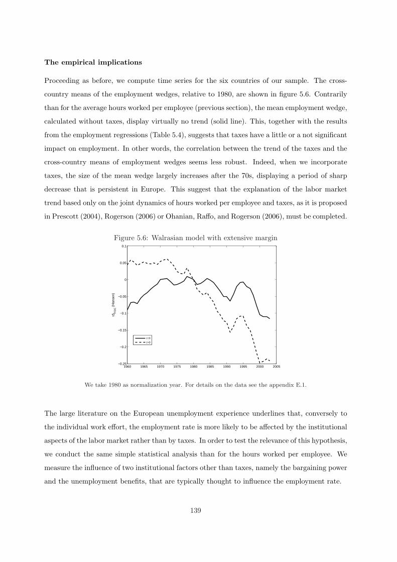
The empirical implications
Proceeding as before, we compute time series for the six countries of our sample. The cross-
country means of the employment wedges, relative to 1980, are shown in figure 5.6. Contrarily
than for the average hours worked per employee (previous section), the mean employment wedge,
calculated without taxes, display virtually no trend (solid line). This, together with the results
from the employment regressions (Table 5.4), suggests that taxes have a little or a not significant
impact on employment. In other words, the correlation between the trend of the taxes and the
cross-country means of employment wedges seems less robust. Indeed, when we incorporate
taxes, the size of the mean wedge largely increases after the 70s, displaying a period of sharp
decrease that is persistent in Europe. This suggest that the explanation of the labor market
trend based only on the joint dynamics of hours worked per employee and taxes, as it is proposed
in Prescott (2004), Rogerson (2006) or Ohanian, Raffo, and Rogerson (2006), must be completed.
Figure 5.6: Walrasian model with extensive margin
1960 1965 1970 1975 1980 1985 1990 1995 2000 2005−0.25
−0.2
−0.15
−0.1
−0.05
0
0.05
0.1
r∆F
OC
(H
anse
n)
τ=0
τ>0
We take 1980 as normalization year. For details on the data see the appendix E.1.
The large literature on the European unemployment experience underlines that, conversely to
the individual work effort, the employment rate is more likely to be affected by the institutional
aspects of the labor market rather than by taxes. In order to test the relevance of this hypothesis,
we conduct the same simple statistical analysis than for the hours worked per employee. We
measure the influence of two institutional factors other than taxes, namely the bargaining power
and the unemployment benefits, that are typically thought to influence the employment rate.
139
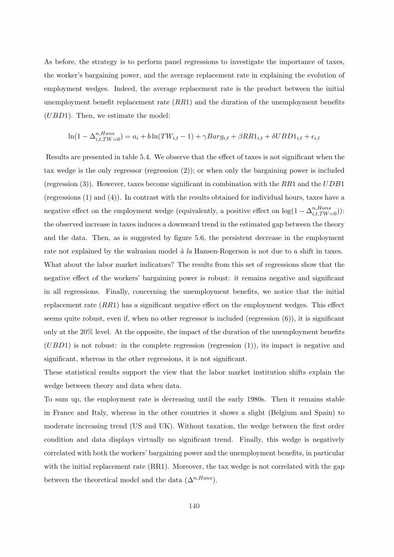
As before, the strategy is to perform panel regressions to investigate the importance of taxes,
the worker’s bargaining power, and the average replacement rate in explaining the evolution of
employment wedges. Indeed, the average replacement rate is the product between the initial
unemployment benefit replacement rate (RR1) and the duration of the unemployment benefits
(UBD1). Then, we estimate the model:
ln(1−∆n,Hansi,t,TW=0) = ai + b ln(TWi,t − 1) + γBargi,t + βRR1i,t + δUBD1i,t + εi,t
Results are presented in table 5.4. We observe that the effect of taxes is not significant when the
tax wedge is the only regressor (regression (2)); or when only the bargaining power is included
(regression (3)). However, taxes become significant in combination with the RR1 and the UDB1
(regressions (1) and (4)). In contrast with the results obtained for individual hours, taxes have a
negative effect on the employment wedge (equivalently, a positive effect on log(1−∆n,Hansi,t,TW=0)):
the observed increase in taxes induces a downward trend in the estimated gap between the theory
and the data. Then, as is suggested by figure 5.6, the persistent decrease in the employment
rate not explained by the walrasian model a la Hansen-Rogerson is not due to a shift in taxes.
What about the labor market indicators? The results from this set of regressions show that the
negative effect of the workers’ bargaining power is robust: it remains negative and significant
in all regressions. Finally, concerning the unemployment benefits, we notice that the initial
replacement rate (RR1) has a significant negative effect on the employment wedges. This effect
seems quite robust, even if, when no other regressor is included (regression (6)), it is significant
only at the 20% level. At the opposite, the impact of the duration of the unemployment benefits
(UBD1) is not robust: in the complete regression (regression (1)), its impact is negative and
significant, whereas in the other regressions, it is not significant.
These statistical results support the view that the labor market institution shifts explain the
wedge between theory and data when data.
To sum up, the employment rate is decreasing until the early 1980s. Then it remains stable
in France and Italy, whereas in the other countries it shows a slight (Belgium and Spain) to
moderate increasing trend (US and UK). Without taxation, the wedge between the first order
condition and data displays virtually no significant trend. Finally, this wedge is negatively
correlated with both the workers’ bargaining power and the unemployment benefits, in particular
with the initial replacement rate (RR1). Moreover, the tax wedge is not correlated with the gap
between the theoretical model and the data (∆n,Hans).
140
Table 5.4: Regression results for the employment, 1980-2003
Reg (1) Reg (2) Reg (3) Reg (4) Reg (5) Reg (6) Reg (7)
abe -0.4583 -1.2336 -.7994 -1.184 -.7722 -1.173 -.5567
[-.8418;-.0748] [-1.282;-1.184] [-1.151;-.4479] [-1.250;-1.118] [-1.120;-.4234] [-1.239;-1.107] [-.9457;-.1676]
asp -0.7522 -1.3145 -1.065 -1.215 -1.071 -1.274 -.9005
[-1.008;-.4962] [-1.339;-1.289] [-1.266;-.8638] [-1.305;-1.125] [-1.272;-.8700] [-1.345;-1.202] [-1.143;-.6578]
afr -0.6809 -1.2328 -.9380 -1.183 -.9084 -1.162 -.7313
[-.9509;-.4108] [-1.286;-1.178] [-1.180;-.6956] [-1.252;-1.115] [-1.145;-.6712] [-1.228;-1.096] [-1.007;-.4554]
ait -0.6528 -1.2554 -.8970 -1.237 -.8738 -1.217 -.7179
[-.9607;-.3450] [-1.298;-1.212] [-1.187;-.6065] [-1.284;-1.189] [-1.161;-.5857] [-1.261;-1.173] [-1.031;-.4041]
auk -0.4298 -0.9498 -.6955 -.8817 -.7063 -.9444 -.5812
[-.6770;-.1825] [-.9799;-.9196] [-.9016;-.4895] [-.9607;-.8028] [-.9118;-.5008] [-.9973;-.8915] [-.8130;-.3495]
aus -0.5013 -0.7875 -.6838 -.7154 -.7049 -.7894 -.6307
[-.6368;-.3659] [-.8312;-.7439] [-.7774;-.5903] [-.7962;-.6345] [-.7912;-.6186] [-.8305;-.7484] [-.7372;-.5243]
TW 0.1670 0.0559 .0546 .1234
[.0540; .2801 ] [-.0403; .1522] [-.0397; .1490] [.0067; .2400 ]
Barg -0.9605 -.6021 -.6051 -.8116
[-1.461;-.4598] [-1.085;-.1192] [-1.088;-.1217] [-1.316;-.3064]
RR1 -0.1704 -.1033 -.0662 -.1118
[-.2682;-.0726] [-.1995;-.0072] [-.1570; .0245] [-.2039;-.0197]
UBD1 -0.0619 -.0362 -.0036 -.0155
[-.1212;-.0026] [-.0970; .0246] [-.0567; .0495] [-.0673; .0363]
N 144 144 144 144 144 144 144
R2 .9329 .9268 .9310 .9275 .9310 .9269 .9320
Ordinary least squares regression. “TW” is the tax wedge, “Barg” the bargaining power of the workers, “RR1”
the initial unemployment benefit replacement rate, and “UBD1” the unemployment benefit duration (years).
The confidence intervals (in brackets) are at the 95% level. See details on the data in the appendix E.1.
141

Since 1980, a notable feature of the data is that differences across countries in aggregate hours
are due to quantitatively important differences along the extensive margin and the intensive
margin. Then, it seems relevant to analyze the labor market dynamics taking into account these
two margins. Moreover, in this alternative quantitative model, the introduction of the labor
market institutions is expected to reduce the gap between the marginal cost and the marginal
return of labor. This is done in the search economy developed in next section.
5.3 Search model with intensive and extensive margins
In this section we propose a theoretical framework allowing to explain simultaneously the dy-
namics of the employment and the hours worked per employee. We also need for a theory
explaining the impact of the labor market institutions such as the bargaining power and the
unemployment benefits. The natural candidate is then the matching model, where both em-
ployment and hours are endogenous. With this type of model, we are able to quantify the
relative importance of taxes and of labor market institutions in the total hours dynamics. More
precisely, we expect that our model is able to explain that the dynamics of the hours worked
per employee is mainly accounted by the taxes, whereas the employment dynamics is driven by
the labor market institutions.
5.3.1 The equilibrium matching model
We present in this section a neo-classical growth model where the labor market equilibrium is
determined by a search process and a wage bargaining process. This model is close to the one
analyzed by Andolfatto (1996), Feve and Langot (1996) and Cheron and Langot (2004).
Labor market flows
Employment is predetermined at each time and changes only gradually as workers separate from
jobs, at the exogenous rate s, or unemployed agents find jobs, at the hiring rate Mt. Let Nt and
Vt, respectively be the number of workers and the total number of new jobs made available by
firms, then employment evolves according to
Nt+1 = (1− s)Nt + Mt
with Mt = V ψt (1−Nt)1−ψ, 0 < ψ < 1.
142
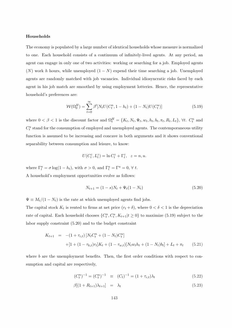
Households
The economy is populated by a large number of identical households whose measure is normalized
to one. Each household consists of a continuum of infinitely-lived agents. At any period, an
agent can engage in only one of two activities: working or searching for a job. Employed agents
(N) work h hours, while unemployed (1 − N) expend their time searching a job. Unemployed
agents are randomly matched with job vacancies. Individual idiosyncratic risks faced by each
agent in his job match are smoothed by using employment lotteries. Hence, the representative
household’s preferences are:
W(ΩH0 ) =
∞∑
t=0
βt[NtU(Cnt , 1− ht) + (1−Nt)U(Cu
t )] (5.19)
where 0 < β < 1 is the discount factor and ΩHt = Kt, Nt, Ψt, wt, ht, bt, πt, Rt, Lt, ∀t. Cn
t and
Cut stand for the consumption of employed and unemployed agents. The contemporaneous utility
function is assumed to be increasing and concave in both arguments and it shows conventional
separability between consumption and leisure, to know:
U(Czt , Lz
t ) = lnCzt + Γz
t , z = n, u.
where Γnt = σ log(1− ht), with σ > 0, and Γu
t = Γu = 0, ∀ t.
A household’s employment opportunities evolve as follows:
Nt+1 = (1− s)Nt + Ψt(1−Nt) (5.20)
Ψ ≡ Mt/(1−Nt) is the rate at which unemployed agents find jobs.
The capital stock Kt is rented to firms at net price (rt + δ), where 0 < δ < 1 is the depreciation
rate of capital. Each household chooses Cnt , Cu
t , Kt+1|t ≥ 0 to maximize (5.19) subject to the
labor supply constraint (5.20) and to the budget constraint
Kt+1 = −(1 + τc,t) [NtCnt + (1−Nt)Cu
t ]
+[1 + (1− τk,t)rt]Kt + (1− τw,t)[Ntwtht + (1−Nt)bt] + Lt + πt (5.21)
where b are the unemployment benefits. Then, the first order conditions with respect to con-
sumption and capital are respectively,
(Cnt )−1 = (Cu
t )−1 ≡ (Ct)−1 = (1 + τc,t)λt (5.22)
β[(1 + Rt+1)λt+1] = λt (5.23)
143
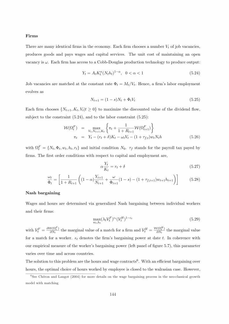
Firms
There are many identical firms in the economy. Each firm chooses a number Vt of job vacancies,
produces goods and pays wages and capital services. The unit cost of maintaining an open
vacancy is ω. Each firm has access to a Cobb-Douglas production technology to produce output:
Yt = AtKαt (Ntht)1−α, 0 < α < 1 (5.24)
Job vacancies are matched at the constant rate Φt = Mt/Vt. Hence, a firm’s labor employment
evolves as
Nt+1 = (1− s)Nt + ΦtVt (5.25)
Each firm chooses Nt+1,Kt, Vt|t ≥ 0 to maximize the discounted value of the dividend flow,
subject to the constraint (5.24), and to the labor constraint (5.25):
W(ΩFt ) = max
Vt,Nt+1,Kt
πt +
11 + Rt+1
W(ΩFt+1)
πt = Yt − (rt + δ)Kt − ωtVt − (1 + τf,t)wtNth (5.26)
with ΩFt = Nt,Φt, wt, ht, rt and initial condition N0. τf stands for the payroll tax payed by
firms. The first order conditions with respect to capital and employment are,
αYt
Kt= rt + δ (5.27)
ωt
Φt=
[1
1 + Rt+1
((1− α)
Yt+1
Nt+1+
ω
Φt+1(1− s)− (1 + τf,t+1)wt+1ht+1
)](5.28)
Nash bargaining
Wages and hours are determined via generalized Nash bargaining between individual workers
and their firms:
maxwt,ht
(λtVFt )εt(VH
t )1−εt (5.29)
with VFt = ∂W(ΩF
t )∂Nt
the marginal value of a match for a firm and VHt = W(ΩH
t )∂Nt
the marginal value
for a match for a worker. εt denotes the firm’s bargaining power at date t. In coherence with
our empirical measure of the worker’s bargaining power (left panel of figure 5.7), this parameter
varies over time and across countries.
The solution to this problem are the hours and wage contracts6. With an efficient bargaining over
hours, the optimal choice of hours worked by employee is closed to the walrasian case. However,6See Cheron and Langot (2004) for more details on the wage bargaining process in the neo-classical growth
model with matching
144
the wage contract takes into account the dynamic behavior of taxes and the unemployment
benefits.
The Equilibrium
Given the vector of taxes, unemployment benefits and bargaining powers τc,t, τf,t, τw,t, bt, εt,the general equilibrium is defined by the set of functions Ct, Vt,Kt+1, Nt+1, wt, ht, Lt,Mt, Yt∞t=0,
solution of the system formed by the optimality conditions, the equation of the employment
dynamics and the condition for the equilibrium on the goods markets. Let define the market
tightness as θt = Vt/(1 − Nt). Finally, to simplify notation, we define the employment tax:
τnt ≡ 1+τf,t
1−τw,t, and the relative bargaining power: χt ≡ 1−εt
εt. Then the system defining the
equilibrium is:
Nt+1 = (1− s)Nt + Mt (5.30)
Mt = θψt (1−Nt) (5.31)
Yt = Kt+1 − (1− δ)Kt + Ct + ωVt (5.32)
Lt = τc,tCt + (τf,t + τw,t)wthtNt + τk,trtKt − b(1− τw,t)(1−Nt) (5.33)
Yt = AtKαt (htNt)1−α (5.34)
1 = β
[λt+1
λt
(1 + (1− τk,t+1)
(α
Yt+1
Kt+1− δ
))](5.35)
ω
Φt= β
[λt+1
λt
((1− α)
Yt+1
Nt+1+ (1− s)
ω
Φt+1− (1 + τf,t+1)wt+1ht+1
)](5.36)
((1 + τc,t)Ct)−1 = λt (5.37)
(1− α)Yt
Ntht=
1 + τf,t
1− τw,t
σ(1− ht)−1
λt(5.38)
wtht =1− εt
1 + τf,t
(1− α)
Yt
Nt+
[1− s
Φt
(1− χt+1
χt
τnt
τnt+1
)+
χt+1
χt
τnt
τnt+1
θt
]ω
(5.39)
+εt
1− τw,t
Γu − Γn
t
λt+ (1− τw,t)bt
Finally, the unemployment benefits are computed as the product of the average replacement
rate (ρt) and the hourly wage: bt = ρtwtht. The last equation can be rewritten as follows:
(1 + τf,t)wtht =1− εt
1− εtρt
(1− α)
Yt
Nt+
[1− s
Φt
(1− χt+1
χt
τnt
τnt+1
)+
χt+1
χt
τnt
τnt+1
θt
]ω
+εt
1− εtρt(1 + TWt)(Γu − Γn
t )Ct
145
In the matching model, both the number of employees and the number of hours worked are
endogenous. After the wage bargaining process, the right to manage assumption leads the firms
to hire a number of workers given a bargained labor cost per employee ((1+ τf,t)wtht). Because
we assume an efficient bargaining process, the equilibrium number of hours is determined by
the same equation than in a walrasian economy (endogenous intensive margin). Then the labor
market equilibrium conditions are:
(1 + τf,t)wtht︸ ︷︷ ︸MCN
= (1− εt)
(1− α)Yt
Nt+
search cost (SC)︷ ︸︸ ︷[1− s
Φt
(1− χt+1
χt
τnt
τnt+1
)+
χt+1
χt
τnt
τnt+1
θt
]ω
︸ ︷︷ ︸Bargained surplus (BS)
+ εt
(1 + TWt)
MRS(N/C)︷ ︸︸ ︷(Γu − Γn
t )Ct +
UB︷ ︸︸ ︷(1 + τf,t)bt
︸ ︷︷ ︸Reservation wage (RW)
(1 + τf,t)wtht︸ ︷︷ ︸MRN
= (1− α)Yt
Nt︸ ︷︷ ︸Instantaneous returns
+ (1− s)ω
Φt−
(1 + τc,t)Ct
β(1 + τc,t−1)Ct−1
ω
Φt−1︸ ︷︷ ︸Intertemporal returns
(1− α)Yt
Ntht︸ ︷︷ ︸MPH
=
(1 + τf,t)(1 + τc,t)1− τw,t
︸ ︷︷ ︸1+TW
σ(1− ht)−1Ct︸ ︷︷ ︸MRS(H/C)
where MRN denotes the marginal return of an employee and MCN her marginal cost. Similarly,
MRS(N/C) denotes the marginal rate of substitution between employment and consumption
whereas MPH stands for the marginal product of an hour worked. The previous system can be
rewritten as:
MRNt = MCNt
MPHt = (1 + TWt)×MRS(H/C)t
One can remark that the MCN has now two components: the bargained surplus and the
reservation wage. Whereas the reservation wage is only affected by the tax/benefit system (tax
wedge and unemployment benefits), the bargained surplus is also affected by the labor market
frictions through the search cost.
Without taxes and without labor market institutions, i.e. TW = 1− ε = UB = 0, the marginal
cost of employment MCN is given by the marginal rate of substitution between employment
146
and consumption MRS(N/C), as in the Hansen-Rogerson economy. Relatively to this walrasian
model, the labor market institutions lead to an increase in the MCN , through the introduction
of both an additional value of leisure (the unemployment benefits UB > 0) and a bargained
surplus (1 − ε > 0). Hence, the shift across time of the labor market institutions can explain
the dynamics of the employment by decreasing the wedge between the data and the theory.
Finally, the increase in the tax wedge TW raises also the marginal cost of employment through
the reservation wage. Via this last channel, one can also expect to reduce the gap between data
and theory.
Following Ohanian, Raffo and Rogerson (2006), we compute the gap between the return and
the cost of the marginal employee as follows:
MCNt = (1−∆nt )MRNt for TW ≥ 0, UB ≥ 0 ⇒ ∆n
t = 1− MCNt
MRNt
Relatively to the Hansen-Rogerson’s economy, the matching model leads to new evaluations of
both the marginal return of employment (MRN) and the marginal cost of employment (MCN).
The smaller the labor market frictions, the smaller is the gap between the Hansen-Rogerson
economy and our matching model.
The condition allowing to generate the number of hours worked in the non-walrasian economy
is the same than in the walrasian one, except that in the previous case the employment rate is
not restricted to be equal to one. This expression does not introduce any labor market friction
because we assume an efficient bargaining process over the hours worked. Then we have:
(1+TWt)MRS(H/C)t = (1−∆ht )MPHt for TW ≥ 0, UB ≥ 0 ⇒ ∆h
t = 1−(1+TWt)MRS(H/C)t
MPHt
Contrary to the walrasian case, we do not impose Nt = 1 (full-employment). The measure of
∆ht is computed using the aggregate production per capita Yt, the aggregate consumption per
capita Ct, the number of hours worked by employee ht and the employment rate Nt.
5.3.2 Calibration and data
The aim of the empirical part is to measure the contribution of both the labor market indicators
(LMI) and the taxes specific of each country. Taxes and LMI were not constant over the last
two decades (see figure 5.7 and figure 5.9). Then, the dynamics of the gap between the marginal
cost of employment and its marginal return is affected by changes in either the LMI and the
taxes. In order to measure the impact of the tax/benefit system we construct the different hours
and employment wedges under several configurations, using the data described in appendix E.1.
147
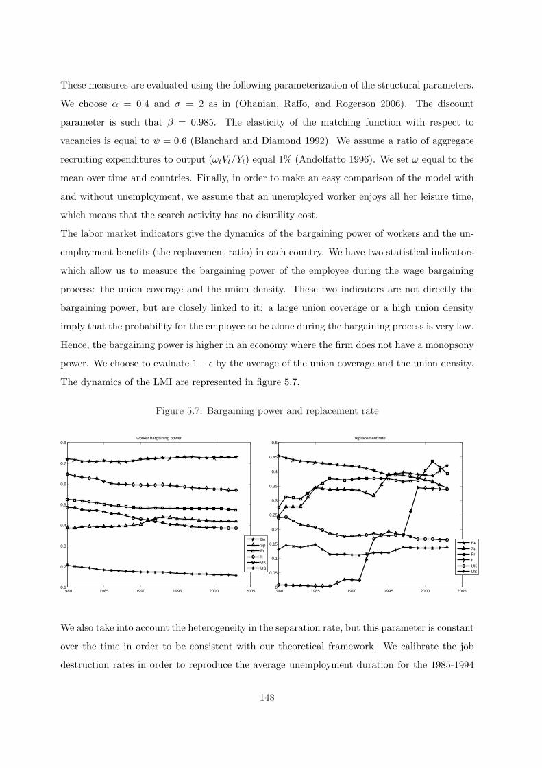
These measures are evaluated using the following parameterization of the structural parameters.
We choose α = 0.4 and σ = 2 as in (Ohanian, Raffo, and Rogerson 2006). The discount
parameter is such that β = 0.985. The elasticity of the matching function with respect to
vacancies is equal to ψ = 0.6 (Blanchard and Diamond 1992). We assume a ratio of aggregate
recruiting expenditures to output (ωtVt/Yt) equal 1% (Andolfatto 1996). We set ω equal to the
mean over time and countries. Finally, in order to make an easy comparison of the model with
and without unemployment, we assume that an unemployed worker enjoys all her leisure time,
which means that the search activity has no disutility cost.
The labor market indicators give the dynamics of the bargaining power of workers and the un-
employment benefits (the replacement ratio) in each country. We have two statistical indicators
which allow us to measure the bargaining power of the employee during the wage bargaining
process: the union coverage and the union density. These two indicators are not directly the
bargaining power, but are closely linked to it: a large union coverage or a high union density
imply that the probability for the employee to be alone during the bargaining process is very low.
Hence, the bargaining power is higher in an economy where the firm does not have a monopsony
power. We choose to evaluate 1− ε by the average of the union coverage and the union density.
The dynamics of the LMI are represented in figure 5.7.
Figure 5.7: Bargaining power and replacement rate
1980 1985 1990 1995 2000 20050.1
0.2
0.3
0.4
0.5
0.6
0.7
0.8worker bargaining power
BeSpFrItUKUS
1980 1985 1990 1995 2000 20050
0.05
0.1
0.15
0.2
0.25
0.3
0.35
0.4
0.45
0.5replacement rate
BeSpFrItUKUS
We also take into account the heterogeneity in the separation rate, but this parameter is constant
over the time in order to be consistent with our theoretical framework. We calibrate the job
destruction rates in order to reproduce the average unemployment duration for the 1985-1994
148
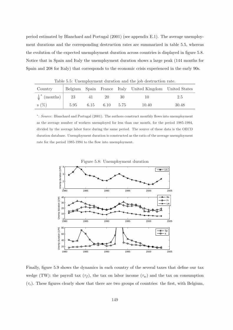
period estimated by Blanchard and Portugal (2001) (see appendix E.1). The average unemploy-
ment durations and the corresponding destruction rates are summarized in table 5.5, whereas
the evolution of the expected unemployment duration across countries is displayed in figure 5.8.
Notice that in Spain and Italy the unemployment duration shows a large peak (144 months for
Spain and 208 for Italy) that corresponds to the economic crisis experienced in the early 90s.
Table 5.5: Unemployment duration and the job destruction rate.
Country Belgium Spain France Italy United Kingdom United States1Ψ
∗ (months) 23 41 20 30 10 2.5
s (%) 5.95 6.15 6.10 5.75 10.40 30.48
∗: Source: Blanchard and Portugal (2001). The authors construct monthly flows into unemployment
as the average number of workers unemployed for less than one month, for the period 1985-1994,
divided by the average labor force during the same period. The source of these data is the OECD
duration database. Unemployment duration is constructed as the ratio of the average unemployment
rate for the period 1985-1994 to the flow into unemployment.
Figure 5.8: Unemployment duration
1980 1985 1990 1995 2000 20051
2
3
4
Une
mp
dura
tion
(1/Ψ
)
US
1980 1985 1990 1995 2000 20050
10
20
30
40
Une
mp
dura
tion
(1/Ψ
)
BeFrUK
1980 1985 1990 1995 2000 2005
20
40
60
80
Une
mp
dura
tion
(1/Ψ
)
SpIt
Finally, figure 5.9 shows the dynamics in each country of the several taxes that define our tax
wedge (TW): the payroll tax (τf ), the tax on labor income (τw) and the tax on consumption
(τc). These figures clearly show that there are two groups of countries: the first, with Belgium,
149
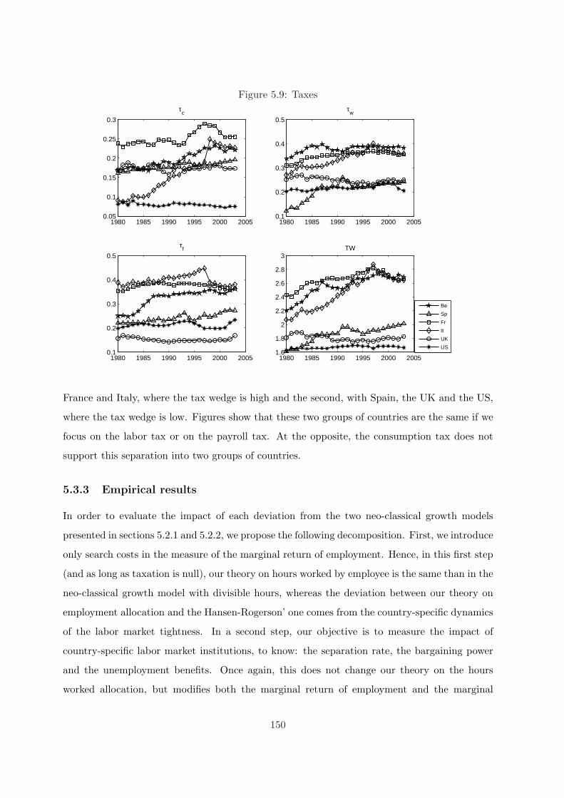
Figure 5.9: Taxes
1980 1985 1990 1995 2000 20050.05
0.1
0.15
0.2
0.25
0.3
τc
Be
Sp
Fr
It
UK
US
1980 1985 1990 1995 2000 20050.1
0.2
0.3
0.4
0.5
τw
1980 1985 1990 1995 2000 20050.1
0.2
0.3
0.4
0.5
τf
1980 1985 1990 1995 2000 20051.6
1.8
2
2.2
2.4
2.6
2.8
3TW
France and Italy, where the tax wedge is high and the second, with Spain, the UK and the US,
where the tax wedge is low. Figures show that these two groups of countries are the same if we
focus on the labor tax or on the payroll tax. At the opposite, the consumption tax does not
support this separation into two groups of countries.
5.3.3 Empirical results
In order to evaluate the impact of each deviation from the two neo-classical growth models
presented in sections 5.2.1 and 5.2.2, we propose the following decomposition. First, we introduce
only search costs in the measure of the marginal return of employment. Hence, in this first step
(and as long as taxation is null), our theory on hours worked by employee is the same than in the
neo-classical growth model with divisible hours, whereas the deviation between our theory on
employment allocation and the Hansen-Rogerson’ one comes from the country-specific dynamics
of the labor market tightness. In a second step, our objective is to measure the impact of
country-specific labor market institutions, to know: the separation rate, the bargaining power
and the unemployment benefits. Once again, this does not change our theory on the hours
worked allocation, but modifies both the marginal return of employment and the marginal
150
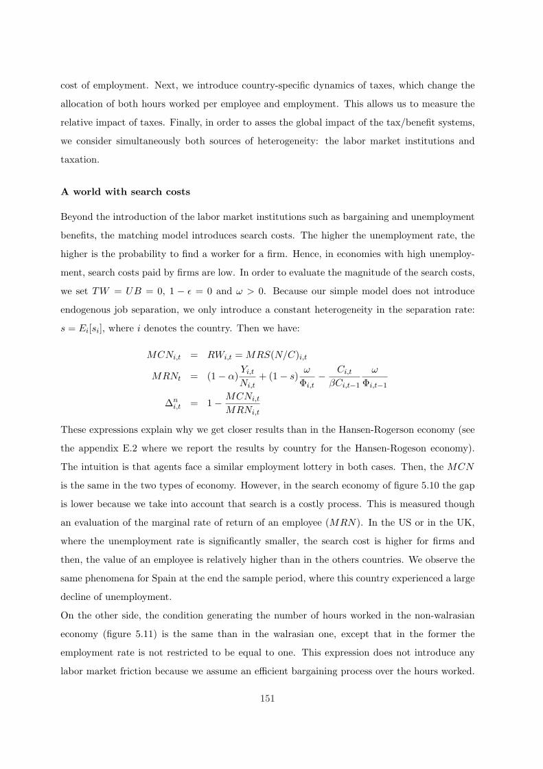
cost of employment. Next, we introduce country-specific dynamics of taxes, which change the
allocation of both hours worked per employee and employment. This allows us to measure the
relative impact of taxes. Finally, in order to asses the global impact of the tax/benefit systems,
we consider simultaneously both sources of heterogeneity: the labor market institutions and
taxation.
A world with search costs
Beyond the introduction of the labor market institutions such as bargaining and unemployment
benefits, the matching model introduces search costs. The higher the unemployment rate, the
higher is the probability to find a worker for a firm. Hence, in economies with high unemploy-
ment, search costs paid by firms are low. In order to evaluate the magnitude of the search costs,
we set TW = UB = 0, 1 − ε = 0 and ω > 0. Because our simple model does not introduce
endogenous job separation, we only introduce a constant heterogeneity in the separation rate:
s = Ei[si], where i denotes the country. Then we have:
MCNi,t = RWi,t = MRS(N/C)i,t
MRNt = (1− α)Yi,t
Ni,t+ (1− s)
ω
Φi,t− Ci,t
βCi,t−1
ω
Φi,t−1
∆ni,t = 1− MCNi,t
MRNi,t
These expressions explain why we get closer results than in the Hansen-Rogerson economy (see
the appendix E.2 where we report the results by country for the Hansen-Rogeson economy).
The intuition is that agents face a similar employment lottery in both cases. Then, the MCN
is the same in the two types of economy. However, in the search economy of figure 5.10 the gap
is lower because we take into account that search is a costly process. This is measured though
an evaluation of the marginal rate of return of an employee (MRN). In the US or in the UK,
where the unemployment rate is significantly smaller, the search cost is higher for firms and
then, the value of an employee is relatively higher than in the others countries. We observe the
same phenomena for Spain at the end the sample period, where this country experienced a large
decline of unemployment.
On the other side, the condition generating the number of hours worked in the non-walrasian
economy (figure 5.11) is the same than in the walrasian one, except that in the former the
employment rate is not restricted to be equal to one. This expression does not introduce any
labor market friction because we assume an efficient bargaining process over the hours worked.
151
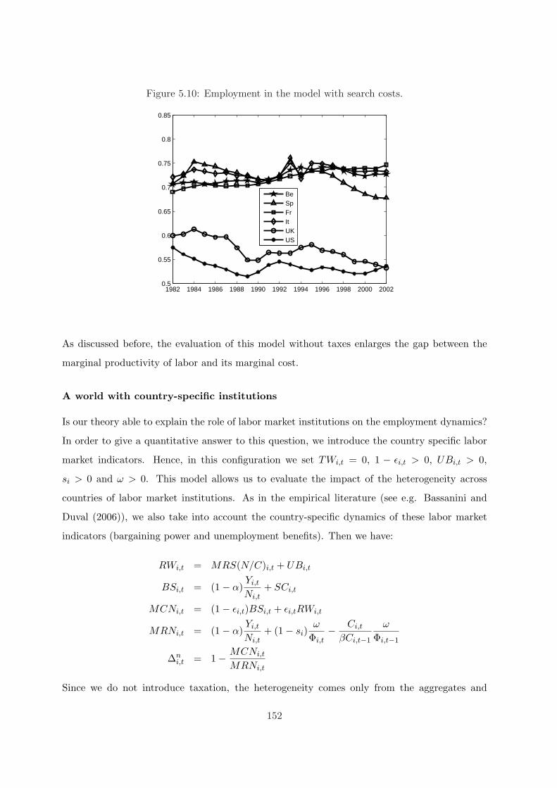
Figure 5.10: Employment in the model with search costs.
1982 1984 1986 1988 1990 1992 1994 1996 1998 2000 20020.5
0.55
0.6
0.65
0.7
0.75
0.8
0.85
BeSpFrItUKUS
As discussed before, the evaluation of this model without taxes enlarges the gap between the
marginal productivity of labor and its marginal cost.
A world with country-specific institutions
Is our theory able to explain the role of labor market institutions on the employment dynamics?
In order to give a quantitative answer to this question, we introduce the country specific labor
market indicators. Hence, in this configuration we set TWi,t = 0, 1 − εi,t > 0, UBi,t > 0,
si > 0 and ω > 0. This model allows us to evaluate the impact of the heterogeneity across
countries of labor market institutions. As in the empirical literature (see e.g. Bassanini and
Duval (2006)), we also take into account the country-specific dynamics of these labor market
indicators (bargaining power and unemployment benefits). Then we have:
RWi,t = MRS(N/C)i,t + UBi,t
BSi,t = (1− α)Yi,t
Ni,t+ SCi,t
MCNi,t = (1− εi,t)BSi,t + εi,tRWi,t
MRNi,t = (1− α)Yi,t
Ni,t+ (1− si)
ω
Φi,t− Ci,t
βCi,t−1
ω
Φi,t−1
∆ni,t = 1− MCNi,t
MRNi,t
Since we do not introduce taxation, the heterogeneity comes only from the aggregates and
152
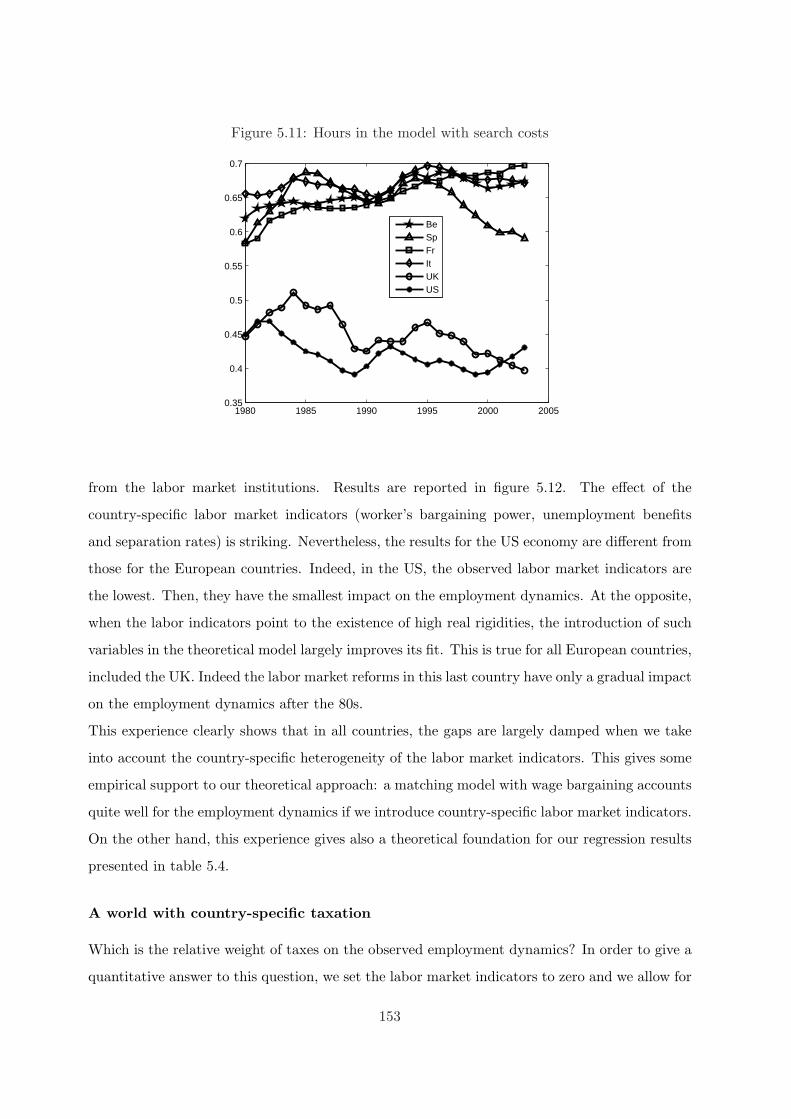
Figure 5.11: Hours in the model with search costs
1980 1985 1990 1995 2000 20050.35
0.4
0.45
0.5
0.55
0.6
0.65
0.7
BeSpFrItUKUS
from the labor market institutions. Results are reported in figure 5.12. The effect of the
country-specific labor market indicators (worker’s bargaining power, unemployment benefits
and separation rates) is striking. Nevertheless, the results for the US economy are different from
those for the European countries. Indeed, in the US, the observed labor market indicators are
the lowest. Then, they have the smallest impact on the employment dynamics. At the opposite,
when the labor indicators point to the existence of high real rigidities, the introduction of such
variables in the theoretical model largely improves its fit. This is true for all European countries,
included the UK. Indeed the labor market reforms in this last country have only a gradual impact
on the employment dynamics after the 80s.
This experience clearly shows that in all countries, the gaps are largely damped when we take
into account the country-specific heterogeneity of the labor market indicators. This gives some
empirical support to our theoretical approach: a matching model with wage bargaining accounts
quite well for the employment dynamics if we introduce country-specific labor market indicators.
On the other hand, this experience gives also a theoretical foundation for our regression results
presented in table 5.4.
A world with country-specific taxation
Which is the relative weight of taxes on the observed employment dynamics? In order to give a
quantitative answer to this question, we set the labor market indicators to zero and we allow for
153
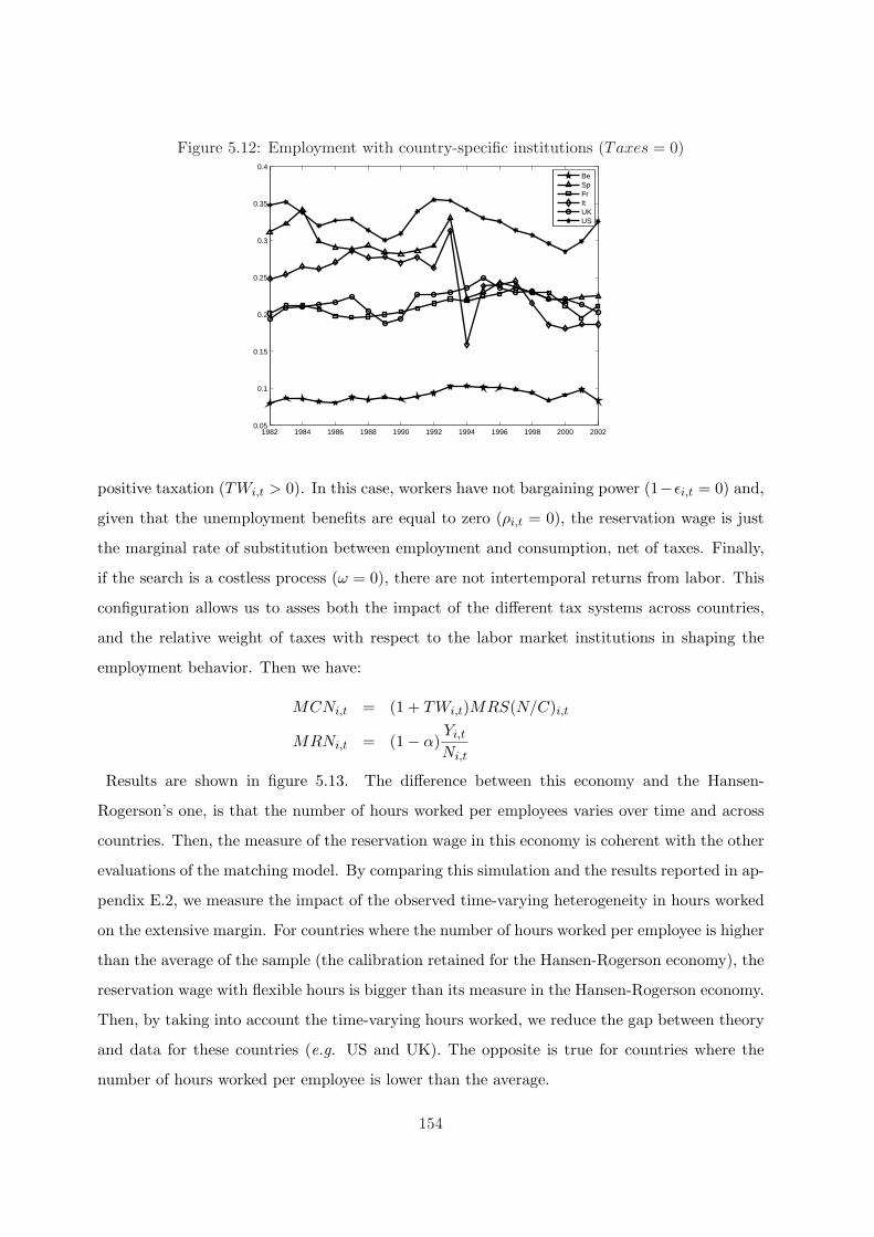
Figure 5.12: Employment with country-specific institutions (Taxes = 0)
1982 1984 1986 1988 1990 1992 1994 1996 1998 2000 20020.05
0.1
0.15
0.2
0.25
0.3
0.35
0.4
BeSpFrItUKUS
positive taxation (TWi,t > 0). In this case, workers have not bargaining power (1−εi,t = 0) and,
given that the unemployment benefits are equal to zero (ρi,t = 0), the reservation wage is just
the marginal rate of substitution between employment and consumption, net of taxes. Finally,
if the search is a costless process (ω = 0), there are not intertemporal returns from labor. This
configuration allows us to asses both the impact of the different tax systems across countries,
and the relative weight of taxes with respect to the labor market institutions in shaping the
employment behavior. Then we have:
MCNi,t = (1 + TWi,t)MRS(N/C)i,t
MRNi,t = (1− α)Yi,t
Ni,t
Results are shown in figure 5.13. The difference between this economy and the Hansen-
Rogerson’s one, is that the number of hours worked per employees varies over time and across
countries. Then, the measure of the reservation wage in this economy is coherent with the other
evaluations of the matching model. By comparing this simulation and the results reported in ap-
pendix E.2, we measure the impact of the observed time-varying heterogeneity in hours worked
on the extensive margin. For countries where the number of hours worked per employee is higher
than the average of the sample (the calibration retained for the Hansen-Rogerson economy), the
reservation wage with flexible hours is bigger than its measure in the Hansen-Rogerson economy.
Then, by taking into account the time-varying hours worked, we reduce the gap between theory
and data for these countries (e.g. US and UK). The opposite is true for countries where the
number of hours worked per employee is lower than the average.
154
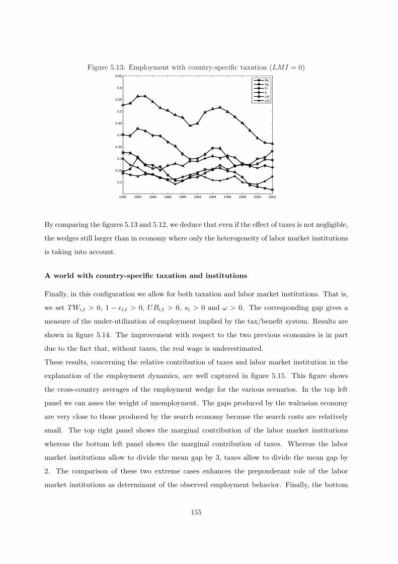
Figure 5.13: Employment with country-specific taxation (LMI = 0)
1982 1984 1986 1988 1990 1992 1994 1996 1998 2000 2002
0.2
0.25
0.3
0.35
0.4
0.45
0.5
0.55
0.6
0.65
BeSpFrItUKUS
By comparing the figures 5.13 and 5.12, we deduce that even if the effect of taxes is not negligible,
the wedges still larger than in economy where only the heterogeneity of labor market institutions
is taking into account.
A world with country-specific taxation and institutions
Finally, in this configuration we allow for both taxation and labor market institutions. That is,
we set TWi,t > 0, 1 − εi,t > 0, UBi,t > 0, si > 0 and ω > 0. The corresponding gap gives a
measure of the under-utilization of employment implied by the tax/benefit system. Results are
shown in figure 5.14. The improvement with respect to the two previous economies is in part
due to the fact that, without taxes, the real wage is underestimated.
These results, concerning the relative contribution of taxes and labor market institution in the
explanation of the employment dynamics, are well captured in figure 5.15. This figure shows
the cross-country averages of the employment wedge for the various scenarios. In the top left
panel we can asses the weight of unemployment. The gaps produced by the walrasian economy
are very close to those produced by the search economy because the search costs are relatively
small. The top right panel shows the marginal contribution of the labor market institutions
whereas the bottom left panel shows the marginal contribution of taxes. Whereas the labor
market institutions allow to divide the mean gap by 3, taxes allow to divide the mean gap by
2. The comparison of these two extreme cases enhances the preponderant role of the labor
market institutions as determinant of the observed employment behavior. Finally, the bottom
155
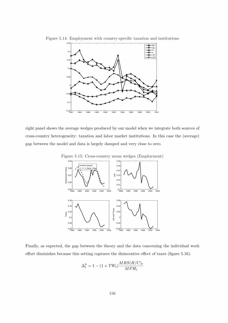
Figure 5.14: Employment with country-specific taxation and institutions
1982 1984 1986 1988 1990 1992 1994 1996 1998 2000 2002−0.15
−0.1
−0.05
0
0.05
0.1
0.15
0.2
0.25
BeSpFrItUKUS
right panel shows the average wedges produced by our model when we integrate both sources of
cross-country heterogeneity: taxation and labor market institutions. In this case the (average)
gap between the model and data is largely damped and very close to zero.
Figure 5.15: Cross-country mean wedges (Employment)
1980 1985 1990 1995 2000 20050.65
0.66
0.67
0.68
0.69
Em
ploy
men
t lot
tery
searchHans.−Rog
1980 1985 1990 1995 2000 20050.2
0.21
0.22
0.23
0.24
0.25
0.26
LMI
1980 1985 1990 1995 2000 20050.26
0.28
0.3
0.32
0.34
0.36
Tax
es
1980 1985 1990 1995 2000 2005−0.04
−0.02
0
0.02
0.04
0.06
LMI a
nd T
axes
Finally, as expected, the gap between the theory and the data concerning the individual work
effort diminishes because this setting captures the disincentive effect of taxes (figure 5.16).
∆ht = 1− (1 + TWt)
MRS(H/C)t
MPHt
156
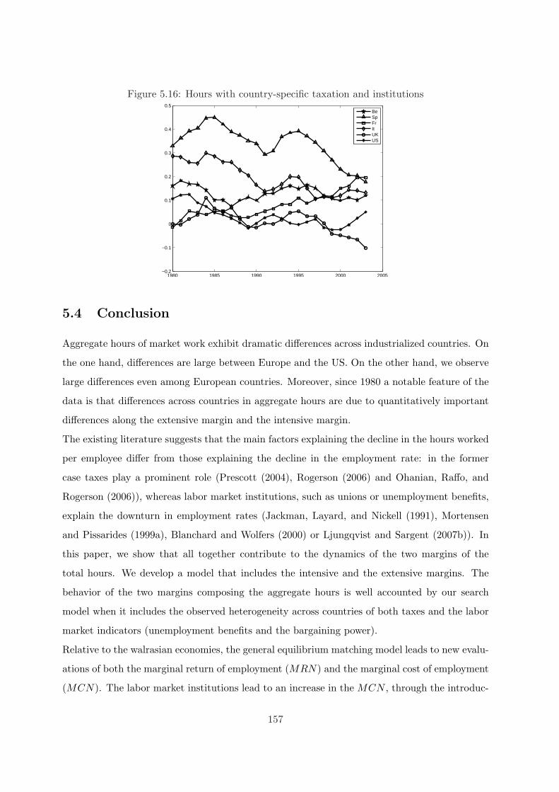
Figure 5.16: Hours with country-specific taxation and institutions
1980 1985 1990 1995 2000 2005−0.2
−0.1
0
0.1
0.2
0.3
0.4
0.5
BeSpFrItUKUS
5.4 Conclusion
Aggregate hours of market work exhibit dramatic differences across industrialized countries. On
the one hand, differences are large between Europe and the US. On the other hand, we observe
large differences even among European countries. Moreover, since 1980 a notable feature of the
data is that differences across countries in aggregate hours are due to quantitatively important
differences along the extensive margin and the intensive margin.
The existing literature suggests that the main factors explaining the decline in the hours worked
per employee differ from those explaining the decline in the employment rate: in the former
case taxes play a prominent role (Prescott (2004), Rogerson (2006) and Ohanian, Raffo, and
Rogerson (2006)), whereas labor market institutions, such as unions or unemployment benefits,
explain the downturn in employment rates (Jackman, Layard, and Nickell (1991), Mortensen
and Pissarides (1999a), Blanchard and Wolfers (2000) or Ljungqvist and Sargent (2007b)). In
this paper, we show that all together contribute to the dynamics of the two margins of the
total hours. We develop a model that includes the intensive and the extensive margins. The
behavior of the two margins composing the aggregate hours is well accounted by our search
model when it includes the observed heterogeneity across countries of both taxes and the labor
market indicators (unemployment benefits and the bargaining power).
Relative to the walrasian economies, the general equilibrium matching model leads to new evalu-
ations of both the marginal return of employment (MRN) and the marginal cost of employment
(MCN). The labor market institutions lead to an increase in the MCN , through the introduc-
157

tion of both an additional value of leisure (the unemployment benefits) and a bargained surplus.
Hence, we show that the shift across time of the labor market institutions explains approxi-
mately 2/3 of the dynamics of the employment rate. The increase of the tax wedge raises also
the marginal cost of employment through the reservation wage. Through this channel, taxes
explain about 1/3 of the employment rate dynamics. Finally, we show that we need only taxes
for accounting for the observed shift in the average hours worked per employee.
In addition, our quantitative experiences put in evidence that the US economy is closer to the
walrasian model than the European economies, because frictions on the labor market are smaller.
Finally, our results suggest than in all cases, the matching model performs better in the labor
market accounting exercise.
158
Conclusion
This dissertation tries to gain insight on the identification of the key factors that shape the
short-run and the long-run evolution of industrialized economies. Can we explain the observed
international fluctuations and the U.S. labor market facts? Can we account for the economic
slowdown of economic growth, and the high unemployment experienced by continental Euro-
pean countries last decades? How to rationalize the dramatic differences across industrialized
countries of the aggregate hours of market work?
This dissertation propose plausible explanations to these issues. In particular, chapter 3 shows
that that fluctuations in distortive taxes can account for some of the puzzling features of the
U.S. business cycle. Namely, the observed real wage rigidity, the international comovement of
investments and labor inputs, and the so-called consumption correlation puzzle (according to
which cross-country correlations of output are higher than the one of consumption). This is
done in a two-country search and matching model with fairly standard preferences, extended to
include a tax/benefit system. In this simple framework, the tax side is represented by taxation
on labor income, employment (payroll tax) and consumption, whereas the benefit side is resumed
by the unemployment benefits and the worker’s bargaining power.
In turn, chapter 4 argues that the link between economic growth and long term unemployment
can be viewed through the simultaneous link of growth and unemployment with the labor mar-
ket institutions. The empirical advises from this chapter are that: (i) The tax wedge and the
unemployment benefits are positively correlated with the regional unemployment rates. Con-
versely, the employment protection and the level of coordination in the wage bargaining process
are negatively correlated with the regional unemployment rates. (ii) The tax wedge and the
unemployment benefits are negatively correlated with the regional growth rates of the Gross
Domestic Product (GDP) per capita. Conversely, more coordination in the wage bargaining
process diminishes the regional growth rates of GDP per capita. This last result points to the
159

existence of an arbitration between unemployment and growth, if we focus on the impact of
coordination in the wage bargaining process. And the implications of the theoretical model
are the following: (i) The bargaining power of unions, the unemployment compensation, the
taxes on labor and the employment protection have a positive effect on unemployment and a
negative effect on the economic growth. (ii) A more coordinated bargaining process increases
employment, at the price of a lower economic growth.
Finally, chapter 5 points to the relevance of taking into account the intensive and the extensive
margins on the labor market to better understand the dynamics of the aggregate hours of market
work. From a theoretical point of view, this chapter also provides a theory allowing to account
for the impact, of both taxes and labor market institutions, on the two margins of the aggregate
hours worked. The main findings are the following. First, the long-run decline in the hours
worked per employee is mainly due to the increase of the taxes, as it is suggested by Prescott
(2004), Rogerson (2006) and Ohanian, Raffo, and Rogerson (2006). Second, the employment
rate is affected by institutional aspects of the labor market, such as the bargaining power and the
unemployment benefits, rather than by taxes, conversely to the individual work effort. Finally,
this behavior of the two margins of the aggregate hours is well accounted by our search model,
when it includes the observed heterogeneity of the tax/benefit systems and the labor market
indicators of the wage-setting process across countries. These findings give some support to the
two explanations of the European decline in total hours: the important role of taxes through
the intensive margin and the large contribution of the labor market institutions through the
extensive margin. Because these findings come from an unified framework, they also give a
strong support to the matching models.
160
Bibliography
Adjemian, S., F. Langot, and C. Quintero-Rojas (2006): “Growth, Unemployment and
Tax/Benefit system in European Countries: Theoretical and Empirical Investigations,” Dis-
cussion Paper SCS8-CT-2004-502639, European Commission, TAXBEN.
Aghion, P., and P. Howitt (1994): “Growth and Unemployment,” Review of Economic
Studies, (61), 477–494.
(1998): Endogenous Growth Theory. MIT.
Alonso, A., C. Echeverria, and K. C. Tran (2004): “Long-Run Economic Performance
and the Labor Market,” Southern Economic Journal, 70(4), 905–919.
Andolfatto, D. (1996): “Business cycle and labor market search,” American Economic Re-
view, 86(1), 112–132.
Arvanitis, V., and A. Mikkola (1996): “Asset market structure and international trade
dynamics,” American Economic Association.
Backus, D. K., P. J. Kehoe, and F. E. Kydland (1992): “International Real Business
Cycles,” Journal of Political Economy, 100(4).
(1994): “Dynamics of the Trade Balance and the Terms of Trade: The J-Curve?,”
American Economic Review, 84(1), 84–103.
(1995): Frontiers of Business Cycle Researchchap. International Business Cycles: The-
ory vs. Evidence. Princeton University Press.
Baldwin, J., T. Dunne, and J. Haltiwanger (1998): “A comparison of Job Creation and
Job Destruction in Canada and the United States,” The Review of Economics and Statistics,
80(3), 347–356.
161
Bassanini, A., and R. Duval (2006): “Employment Patterns in OECD Countries: Reassesing
the Role of Policies and Institutions,” OECD Social, Employment and Migration Working
Papers, 4(35).
Baxter, M. (1995): “International Trade and Business Cycles,” NBER Working Paper Series,
(5025).
Baxter, M., and M. Crucini (1993): “Explaining Saving-Investment Correlations,” American
Economic Review, 83, 416–436.
(1995): “Business Cycles and the Asset Structure of Foreign Trade,” International
Economic Review, 36(4), 821–853.
Bean, C., and C. Pissarides (1993): “Unemployment, consumption and growth,” European
Economic Review, 37, 837–854.
Benhabib, J., R. Rogerson, and R. Wright (1991): “Homework in macroeconomics:
Household production and aggregate fluctuations,” Journal of Political Economy, 99, 1166–
1187.
Berman, E., J. Bound, and S. Machin (1998): “Implications of Skilled-Biased Technological
Change: International Evidence,” Quarterly Journal of Economics, 113, 1245–1280.
Bianconi, M. (1995): “Fiscal policy in a simple two-country dynamic model,” Journal of
Economic Dynamics and Control, 19, 395–419.
Blanchard, O. (2005): “European unemployment: the evolution of facts and ideas,” NBER
Working Paper Series, (11750).
Blanchard, O., and P. Diamond (1992): “The Flow Approach to Labor Markets,” American
Economic Review, 82(2), 501–515.
Blanchard, O., and P. Portugal (2001): “What Hides behind an Unemployment Rate:
Comparing Portuguese and U.S. Labor Markets,” American Economic Review, 91(1), 187–
207.
Blanchard, O., and J. Wolfers (2000): “The role of shocks and institutions in the rise of
european unemployment: the aggregate evidence,” Economic Journal, 110, 1–33.
162
Braun, R. A. (1994): “Tax disturbances and real economic activity in the postwar United
States,” Journal of Monetary Economics, (33), 441–462.
Burnside, C., M. Eichenbaum, and J. D. M. Fisher (2004): “Fiscal shocks and their
consequences,” Journal of Economic Theory, (115), 89–117.
Cardia, E., N. Kozhaya, and F. J. Ruge-Murcia (2003): “Distortionary Taxation and
labor supply,” Journal of Money, Credit and Banking, 35(3), 351–373.
Chari, V. V., P. J. Kehoe, and E. R. McGrattan (2007): “Business Cycle Accounting,”
Econometrica, 75(3), 781–836.
Cheron, A., and F. Langot (2004): “Labor market search and real business cycles: rec-
onciling Nash bargaining with the real wage dynamics,” Review of Economic Dynamics, 7,
476–493.
Christiano, L. J., and M. Eichenbaum (1992): “Current Real Business Cycle Theories and
Aggregate Labor-market Fluctuations,” American Economic Review, (82), 430–450.
Cole, H., and L. Ohanian (2002): “The U.S. and U.K. Great Depressions Through the Lens
of Neoclassical Growth Theory,” American Economic Review, 92(826), 28–32.
Corsetti, G., L. Dedola, and S. Leduc (2004): “International Risk-Sharing and the Trans-
mission of Productivity Shocks,” European Central Bank, (308).
Daveri, F., and G. Tabellini (2000): “Unemployment, growth and taxation in industrial
countries,” Economic Policy, 15(30), 47–104.
Devereux, M., A. Gregory, and G. Smith (1992): “Realistic cross-country consumption
correlation in a two-country, equilibrium, business-cycle model,” Journal of International
Money and Finance.
Faggio, G., and S. Nickell (2006): “Patterns of work across the OECD,” Unpublished.
Feve, P., and F. Langot (1996): “Unemployment and business cycle in a small open economy:
GMM estimation and testing on French data,” Journal of Economic Dynamics and Control,
(20).
Galı, J. (1994): “Monopolistic Competition, Business Cycles, and the Composition of Aggre-
gate Demand,” Journal of Economic Theory, (63), 73–96.
163
Galı, J., M. Gertler, and D. Lopez-Salido (2007): “Markups, Gaps, and the Welfare
Costs of Business Fluctuations,” Review of Economics and Statistics, 89(826), 44–59.
Gomez-Salvador, R., J. Messina, and G. Vallanti (2004): “Gross job flows and institu-
tions in Europe,” Labour Economics, (11), 469–485.
Greene, W. H. (2002): Econometric analysis. Prentice Hall, New Jersey.
Greenwood, J., G. MacDonald, and G. Zhang (1996): “The cyclical behavior of job
creation and job destruction: A sectoral model,” Economic Theory, 7, 95–112.
Grossman, G. E., and E. Helpman (1991): Innovation and Growth in the Global Economy.
MIT.
Grossman, V. (2000): “Skilled Labor Reallocation, Wage Inequality, and Unskilled Unemploy-
ment,” 156, 473–500.
Hairault, J. O. (1995): Advances in Business Cycle Researchchap. Presentation and Evalua-
tion of the Real Business Cycle Approach, pp. 21–54. Springer.
(2002): “Labor Market Search and International Business Cycles,” Review of Economic
Dynamics, 5, 535–558.
Hairault, J. O., F. Langot, and T. Sopraseuth (2007): “The Interaction between Re-
tirement and Job Search: A Global Approach to Older Workers Employment,” Discussion
Paper, Cepremap-PSE, EPEI-Universite d’Evry and GAINS-TEPP-Universite du Maine.
(2008): “Quantifying the Laffer Curve on the Continued Activity Tax in a Dynastic
Framework,” Forthcoming International Economic Review.
Hairault, J. O., and F. Portier (1995): Advances in Business Cycle Researchchap. Nominal
Rigidities and Monopolistic Competition: A New-Keynesian View, pp. 197–240. Springer.
Hansen, G. (1985): “Indivisible Labor and the Business Cycles,” Journal of Monetary Eco-
nomics, 16, 309–327.
Helpman, E., and P. Krugman (1985): Market Structute and Foreign Trade. MIT.
Jackman, N., R. Layard, and S. Nickell (1991): “Unemployment, Macroeconomic Perfor-
mance and the Labour Market,” Oxford University Press.
164
Joines, D. H. (1981): “Estimates of effective marginal tax rates on factor incomes,” The
Journal of Business, 54(2), 191–226.
Jonsson, G., and P. Klein (1996): “Stochastic fiscal policy and the Swedish business cycle,”
Journal of Monetary Economics, 38, 245–268.
Kaitila, V. (2006): “Productivity, hours worked, and Tax/Benefit systems in Europe and
beyond,” Discussion Paper SCS8-CT-2004-502639, European comission, TAXBEN.
Kehoe, P. J., and F. Perri (2000): “International Business Cycle with Endogenous Incom-
plete Markets,” .
King, R., C. Plosser, and S. Rebelo (1988): “Production, Growth and Business Cycles I,”
Journal of Monetary Economics, 21(2/3), 196–232.
Langot, F., and C. Quintero-Rojas (2008): “Explaining the evolution of hours worked
and employment across OECD countries: an equilibrium search approach,” IZA Discussion
Paper, (3364).
Layard, R., and S. Nickell (1999): “Labor market institutions and economic performance,”
Handbook of Labor Economics, 3C. North-Holland, 3029–3084.
Lingens, J. (2003): “The impact of a unionised labor market in a Schumpeterian growth
model,” Labour Economics, (10), 91–104.
Ljungqvist, L., and T. Sargent (2007a): “Understanding European unemployment with a
representative family model,” Journal of Monetary Economics, (54), 2180–2204.
(2007b): “Understanding European unemployment with matching and search-island
models,” Journal of Monetary Economics, (54), 2139–2179.
(2008a): “Taxes, benefits and carees: Complete versus incomplete markets,” Journal
of Monetary Economics, (55), 98–125.
(2008b): “Two Questions about European Unemployment,” Econometrica, 76(1), 1–29.
McDaniel, C. (2007): “Average tax rates on consumption, investment, labor and capital in
the OECD 1950-2003,” Arizona State University, mimeo.
165
McGrattan, E., R. Rogerson, and R. Wright (1997): “An equilibrium model of the
business cycle with household production and fiscal policy,” International Economic Review,
38(2).
McGrattan, E. R. (1994): “The macroeconomic effects of distortionary taxation,” Journal of
Monetary Economics, 33, 573–601.
McIntyre, K. H. (2003): “Can non-traded goods solve the comovement problem?,” Journal
of Macroeconomics, 65, 169–196.
Mendoza, E., A. Razzin, and L. Tessar (1994): “Effective tax rates in macroeconomics:
Cross-country estimates of tax rates on factor incomes and consumption,” Journal of Mone-
tary Economics, (34), 297–323.
Merz, M. (1995): “Search in the labor market and the real business cycle,” Journal of Monetary
Economics, (36), 269–300.
Mortensen, D. T. (2005): “Growth, Unemployment and Labor Market Policy,” The Journal
of the European Economic Association.
Mortensen, D. T., and C. A. Pissarides (1994): “Job creation and job destruction in the
theory of unemployment,” Review of Economic Studies, 61, 397–415.
(1998): “Technical progress, job creation and job destruction,” Review of Economic
Dynamics, 1, 733–753.
(1999a): Job reallocation, employment fluctuations and unemployment,vol. 1 of Hand-
book of Macroeconomics, chap. 18, pp. 1171–1228. North-Holland.
(1999b): “Unemployment Responses to ’Skill-Biased’ Technology Shocks: The Role of
Labour Market Policy,” Economic Journal, 109(455), 242–265.
Ohanian, L., A. Raffo, and R. Rogerson (2006): “Long-term changes in labor supply and
taxes: evidence from OECD countries, 1956-2004,” NBER Working Paper Series, (12786).
Pissarides, C. A. (2000): Equilibrium Unemployment Theory. MIT.
Prescott, E. (2004): “Why do Americans work so much more than Europeans?,” Federal
Reserve Bank of Minneapolis Quarterly Review, 28(1), 2–13.
166
Prescott, E., R. Rogerson, and J. Wallenius (2007): “Lifetime aggregate labor supply
with endogenous worweek length,” Federal Reserve Bank of Minneapolis.
Rogerson, R. (1988): “Indivisible labor, lotteries and equilibrium,” Journal of Monetary
Economics, 22(3), 501–515.
(2006): “Understanding differences in hours worked,” Review of Economic Dynamics,
(9), 365–409.
Rogerson, R., and J. Wallenius (2007): “Micro and macro elasticities in a life cycle model
with taxes,” NBER, (13017).
Rogerson, R., and R. Wright (1988): “Involuntary unemployment in economies with effi-
cient risk sharing,” Journal of Monetary Economics, 22(3), 476–493.
Shi, S., and Q. Wen (1998): “Labor market search and the dynamic effects of taxes and
subsidies,” Journal of Monetary Economics, 43, 457–495.
Sopraseuth, T. (2000): “Dynamique du taux de change et Fluctuations Internationales,”
Ph.D. thesis, Universite de Paris I, Pantheon Sorbonne.
Stockman, A., and L. Tesar (1995): “Tastes and technology in a two-country model of
business cycle: Explaining international comovements,” American Economic Review.
Tripier, F. (2003): “Can the labor market search model explain the fluctuations of allocations
of time?,” Economic Modelling, 21, 131–146.
Ville, K. (2006): “Productivity, hours worked, and Tax/Benefit systems in Europe and be-
yond,” Discussion Paper SCS8-CT-2004-502639, European comission, TAXBEN.
167
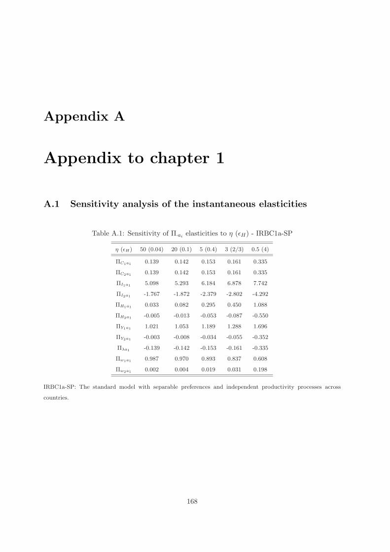
Appendix A
Appendix to chapter 1
A.1 Sensitivity analysis of the instantaneous elasticities
Table A.1: Sensitivity of Π·ai elasticities to η (εH) - IRBC1a-SP
η (εH) 50 (0.04) 20 (0.1) 5 (0.4) 3 (2/3) 0.5 (4)
ΠC1a1 0.139 0.142 0.153 0.161 0.335
ΠC2a1 0.139 0.142 0.153 0.161 0.335
ΠI1a1 5.098 5.293 6.184 6.878 7.742
ΠI2a1 -1.767 -1.872 -2.379 -2.802 -4.292
ΠH1a1 0.033 0.082 0.295 0.450 1.088
ΠH2a1 -0.005 -0.013 -0.053 -0.087 -0.550
ΠY1a1 1.021 1.053 1.189 1.288 1.696
ΠY2a1 -0.003 -0.008 -0.034 -0.055 -0.352
Πλa1 -0.139 -0.142 -0.153 -0.161 -0.335
Πw1a1 0.987 0.970 0.893 0.837 0.608
Πw2a1 0.002 0.004 0.019 0.031 0.198
IRBC1a-SP: The standard model with separable preferences and independent productivity processes across
countries.
168
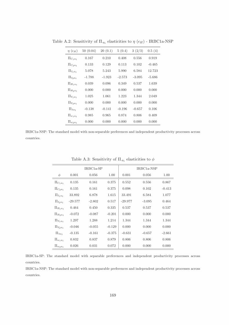
Table A.2: Sensitivity of Π·ai elasticities to η (εH) - IRBC1a-NSP
η (εH) 50 (0.04) 20 (0.1) 5 (0.4) 3 (2/3) 0.5 (4)
ΠC1a1 0.167 0.210 0.408 0.556 0.919
ΠC2a1 0.133 0.129 0.113 0.102 -0.465
ΠI1a1 5.078 5.243 5.990 6.584 12.723
ΠI2a1 -1.788 -1.923 -2.573 -3.095 -5.686
ΠH1a1 0.039 0.096 0.349 0.537 1.639
ΠH2a1 0.000 0.000 0.000 0.000 0.000
ΠY1a1 1.025 1.061 1.223 1.344 2.049
ΠY2a1 0.000 0.000 0.000 0.000 0.000
Πλa1 -0.138 -0.141 -0.196 -0.657 0.106
Πw1a1 0.985 0.965 0.874 0.806 0.409
Πw2a1 0.000 0.000 0.000 0.000 0.000
IRBC1a-NSP: The standard model with non-separable preferences and independent productivity processes across
countries.
Table A.3: Sensitivity of Π·ai elasticities to φ
IRBC1a-SP IRBC1a-NSP
φ 0.001 0.056 1.00 0.001 0.056 1.00
ΠC1a1 0.135 0.161 0.375 0.552 0.556 0.867
ΠC2a1 0.135 0.161 0.375 0.098 0.102 -0.413
ΠI1a1 33.892 6.878 1.615 33.491 6.584 1.077
ΠI2a1 -29.577 -2.802 0.517 -29.977 -3.095 0.464
ΠH1a1 0.464 0.450 0.335 0.537 0.537 0.537
ΠH2a1 -0.072 -0.087 -0.201 0.000 0.000 0.000
ΠY1a1 1.297 1.288 1.214 1.344 1.344 1.344
ΠY2a1 -0.046 -0.055 -0.129 0.000 0.000 0.000
Πλa1 -0.135 -0.161 -0.375 -0.631 -0.657 -2.661
Πw1a1 0.832 0.837 0.879 0.806 0.806 0.806
Πw2a1 0.026 0.031 0.072 0.000 0.000 0.000
IRBC1a-SP: The standard model with separable preferences and independent productivity processes across
countries.
IRBC1a-NSP: The standard model with non-separable preferences and independent productivity processes across
countries.
169
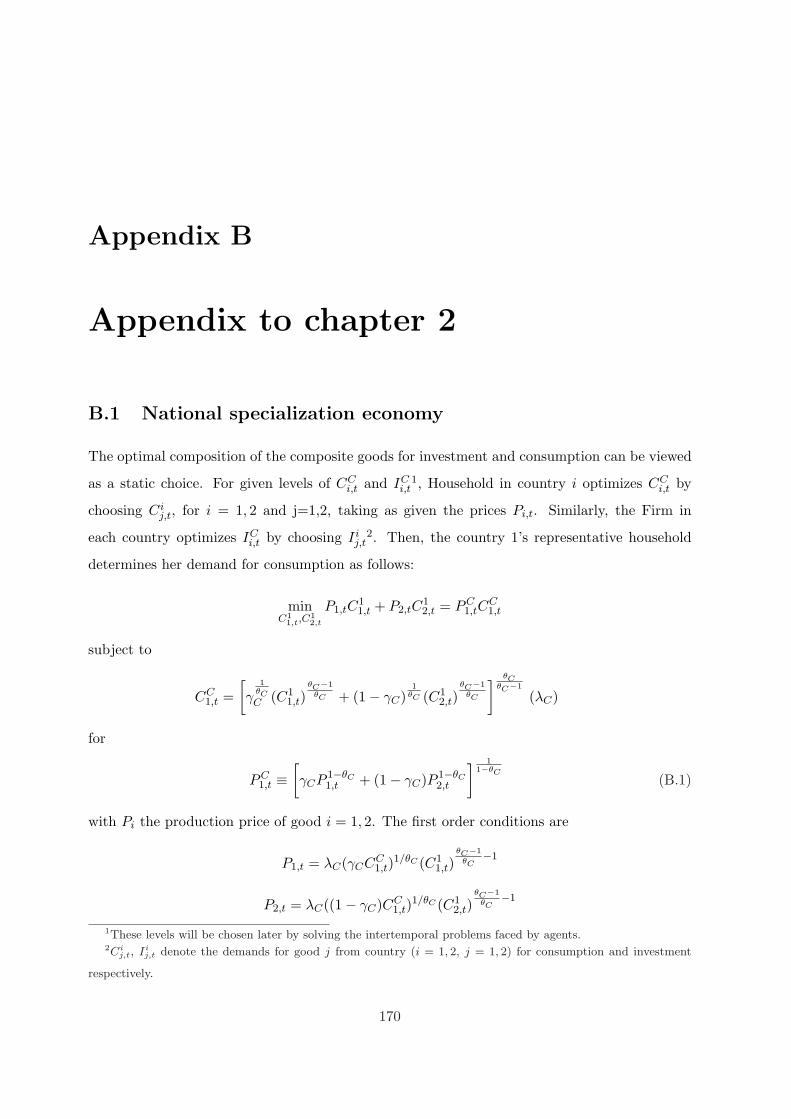
Appendix B
Appendix to chapter 2
B.1 National specialization economy
The optimal composition of the composite goods for investment and consumption can be viewed
as a static choice. For given levels of CCi,t and IC
i,t1, Household in country i optimizes CC
i,t by
choosing Cij,t, for i = 1, 2 and j=1,2, taking as given the prices Pi,t. Similarly, the Firm in
each country optimizes ICi,t by choosing Ii
j,t2. Then, the country 1’s representative household
determines her demand for consumption as follows:
minC1
1,t,C12,t
P1,tC11,t + P2,tC
12,t = PC
1,tCC1,t
subject to
CC1,t =
[γ
1θCC (C1
1,t)θC−1
θC + (1− γC)1
θC (C12,t)
θC−1
θC
] θCθC−1
(λC)
for
PC1,t ≡
[γCP 1−θC
1,t + (1− γC)P 1−θC2,t
] 11−θC
(B.1)
with Pi the production price of good i = 1, 2. The first order conditions are
P1,t = λC(γCCC1,t)
1/θC (C11,t)
θC−1
θC−1
P2,t = λC((1− γC)CC1,t)
1/θC (C12,t)
θC−1
θC−1
1These levels will be chosen later by solving the intertemporal problems faced by agents.2Ci
j,t, Iij,t denote the demands for good j from country (i = 1, 2, j = 1, 2) for consumption and investment
respectively.
170

then,P2,t
P1,t=
(1− γC
γC
)1/θC(
C11,t
C12,t
)1/θC
(B.2)
so,
C11,t =
(γC
1− γC
)(P2,t
P1,t
)θC
C12,t (B.3)
⇐⇒
C12,t =
(1− γC
γC
)(P1,t
P2,t
)θC
C11,t (B.4)
By substituting (33) into the objective one gets
C12,t = (1− γC)
(PC
1,t
P2,t
)θC
CC1,t (B.5)
Similarly, by substituting (34),
C11,t = γC
(PC
1,t
P1,t
)θC
CC1,t (B.6)
In a similar way, the representative household in country 2 determines his demand for consump-
tion by solving
minC2
2,t,C21,t
P1,tC21,t + P2,tC
22,t
subject to
CC2,t =
[γ
1θCC (C2
2,t)θC−1
θC + (1− γC)1
θC (C21,t)
θC−1
θC
] θCθC−1
and given that
PC2t ≡
[(1− γC)P 1−θC
1 + γCP 1−θC2
] 11−θC
(B.7)
Then,P2,t
P1,t=
(γC
1− γC
)1/θC(
C21,t
C22,t
)1/θC
(B.8)
so,
C22,t = γC
(PC
2,t
P2,t
)θC
CC2,t (B.9)
C21,t = (1− γC)
(PC
2,t
P1,t
)θC
CC2,t (B.10)
The problems faced by firms are analogous, but the index prices are in this case
P Ii,t =
[γIP
1−θIi,t + (1− γI)P
1−θIj 6=i,t
] 11−θI
171

Thus, the optimal demands for investment addressed by firm 1 are deduced from
P2,t
P1,t=
(1− γI
γI
)1/θI(
I11,t
I12,t
)1/θI
(B.11)
I12,t = (1− γI)
(P I
1,t
P2,t
)θI
IC1,t (B.12)
I11,t = γI
(P I
1,t
P1,t
)θI
IC1,t (B.13)
while those from Firm 2 are
P2,t
P1,t=
(γI
1− γI
)1/θI(
I21,t
I22,t
)1/θI
(B.14)
I22,t = γI
(P I
2,t
P2,t
)θI
IC2,t (B.15)
I21,t = (1− γI)
(P I
2,t
P1,t
)θI
IC2,t (B.16)
Finally, as in Hairault and Portier (1995), to preserve a simple closing of the model, we assume
that the capital accumulation costs Ci,t are paid by firms through the purchase of a CES basket
with the same parameters as that for investment. The optimal composition of these baskets is
identical to (B.12) , (B.13), (B.15) and (B.16), and the demands for goods j from firm i are
given by
C12,t = (1− γI)
(P I
1,t
P2,t
)θI
C1,t (B.17)
C11,t = γI
(P I
1,t
P1,t
)θI
C1,t (B.18)
C22,t = γI
(P I
2,t
P2,t
)θI
C2,t (B.19)
C21,t = (1− γI)
(P I
2,t
P1,t
)θI
C2,t (B.20)
B.2 Two-sectors economy
172
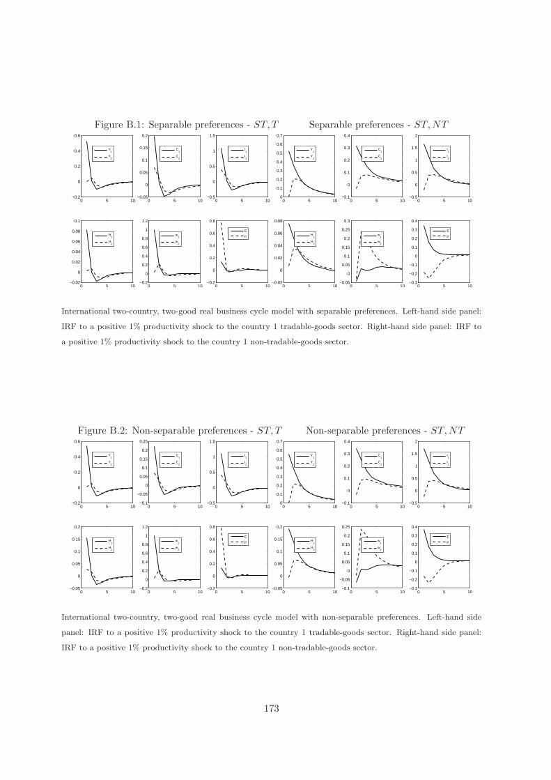
Figure B.1: Separable preferences - ST, T Separable preferences - ST, NT
0 5 10−0.2
0
0.2
0.4
0.6
Y1
Y2
0 5 10−0.05
0
0.05
0.1
0.15
0.2
C1
C2
0 5 10−0.5
0
0.5
1
1.5
I1
I2
0 5 10−0.02
0
0.02
0.04
0.06
0.08
0.1
H1
H2
0 5 10−0.2
0
0.2
0.4
0.6
0.8
1
1.2
w1
w2
0 5 10−0.2
0
0.2
0.4
0.6
0.8
E
p
0 5 100
0.1
0.2
0.3
0.4
0.5
0.6
0.7
Y1
Y2
0 5 10−0.1
0
0.1
0.2
0.3
0.4
C1
C2
0 5 10−0.5
0
0.5
1
1.5
2
I1
I2
0 5 10−0.02
0
0.02
0.04
0.06
0.08
H1
H2
0 5 10−0.05
0
0.05
0.1
0.15
0.2
0.25
0.3
w1
w2
0 5 10−0.3
−0.2
−0.1
0
0.1
0.2
0.3
0.4
E
p
International two-country, two-good real business cycle model with separable preferences. Left-hand side panel:
IRF to a positive 1% productivity shock to the country 1 tradable-goods sector. Right-hand side panel: IRF to
a positive 1% productivity shock to the country 1 non-tradable-goods sector.
Figure B.2: Non-separable preferences - ST, T Non-separable preferences - ST, NT
0 5 10−0.2
0
0.2
0.4
0.6
Y1
Y2
0 5 10−0.1
−0.05
0
0.05
0.1
0.15
0.2
0.25
C1
C2
0 5 10−0.5
0
0.5
1
1.5
I1
I2
0 5 10−0.05
0
0.05
0.1
0.15
0.2
H1
H2
0 5 10−0.2
0
0.2
0.4
0.6
0.8
1
1.2
w1
w2
0 5 10−0.2
0
0.2
0.4
0.6
0.8
E
p
0 5 100
0.1
0.2
0.3
0.4
0.5
0.6
0.7
Y1
Y2
0 5 10−0.1
0
0.1
0.2
0.3
0.4
C1
C2
0 5 10−0.5
0
0.5
1
1.5
2
I1
I2
0 5 10−0.05
0
0.05
0.1
0.15
0.2
H1
H2
0 5 10−0.1
−0.05
0
0.05
0.1
0.15
0.2
0.25
w1
w2
0 5 10−0.3
−0.2
−0.1
0
0.1
0.2
0.3
0.4
E
p
International two-country, two-good real business cycle model with non-separable preferences. Left-hand side
panel: IRF to a positive 1% productivity shock to the country 1 tradable-goods sector. Right-hand side panel:
IRF to a positive 1% productivity shock to the country 1 non-tradable-goods sector.
173

Appendix C
Appendix to chapter 4
C.1 Proofs
Proposition 1. a. ∂g∂i |i=b,τ,τw = h ln(q)∂n
∂i |i=b,τ,τw . It is easy to show that: ∂x∂i |i=b,τ,τw < 0 So,
∂n
∂b= − β1
h(β1b + qhe)
(qh
(1 + τ
1− τw
)x + r + n
)< 0 ⇒
∂g
∂b< 0 and
∂u
∂b= −
(∂x
∂b+
∂n
∂b
)> 0
∂n
∂τ= − q
β1b + qhe
(β1b
1− τw
)x < 0 ⇒ ∂g
∂τ< 0 and
∂u
∂τ> 0
∂n
∂τw= − q
β1b + qhe
(1 + τ
(1− τw)2
)x < 0 ⇒ ∂g
∂τ< 0 and
∂u
∂τ> 0
In a similar way, we deduce: b. ∂x∂e = 0 ⇒
∂g
∂e= − qh ln(q)n
β1b + qhe< 0
∂u
∂e= −∂n
∂e> 0
The first inequality comes from the fact that q > 1.
Proposition 2. Analogous to the proof of proposition 1: ∂x∂β < 0 and ∂n
∂β < 0. So, ∂g∂β < 0 and
∂u∂β > 0.
Proposition 3. It is easy to verify that xE = xβ1
1−α
1 . Since β1 ≥ 1, then x ≤ xE . On the
other hand, πE ≤ π. This is due to the decreasing returns of the technology. Then, nE ≤ n ⇒gE ≤ g. Because there are less researchers but more employed in production the total effect on
u is ambiguous.
174

Appendix D
Reaching the Optimal Growth:
Which is the role of the Labor
Market Institutions?
In this part, we make a social welfare exercise using a simplified version of the general equilibrium
model of endogenous growth developed in chapter 4. We show that the optimal growth rate can
be reached by compensating the distortions on the goods-sector due to the growth process with
the distortions induced by the labor market rigidities.
Introduction
Creative destruction in the economic growth process could lead either to insufficient or excessive
economic growth (Aghion and Howitt 1998). This is mainly explained by the distortions on
the goods-sector induced by the monopolistic rents generated by R&D. However, we show that
when the institutions and rigidities present in the labor market of many developed economies
are acknowledged by the model, the optimal growth rate could be reached. Specifically, when
the economic growth is excessive, the labor market rigidities are desirable because its negative
impact on growth reduce the gap to the optimal rate. Conversely, when the economic growth is
suboptimal, the fiscal policy gives the solution: the optimal rate can be reached by subsidizing
labor.
175
D.1 The model
The basics of the model are: (i) Innovations are the engine of growth. (ii) Agents have the choice
of being employed or doing research and development activities (R&D). (iii) Unemployment is
caused both by the wage-setting behavior of the unions representing the workers’ interests, and
by the labor costs associated to taxes and unemployment compensation.
D.1.1 Preferences
The economy is populated by L identical agents, each endowed with one unit flow of labor.
At each time, they may be employed (x), trying their hand at R&D (n) or unemployed (u):
L = x + n + u. When employed, workers pay a tax τw on their labor income.
All individuals have the same linear preferences over lifetime consumption C of a single final
good:
U(C) = E0
∫ ∞
0C(t)e−ρtdt (D.1)
ρ > 0 is the subjective rate of time preference and Ct is the individual’s consumption of the
final good at time t.
D.1.2 Goods sector
The final good is produced by perfectly competitive firms that use the latest vintage v of inter-
mediate input x,1
C(t) = Av,txαv,t, 0 < α < 1 (D.2)
Av represents the productivity of the intermediate good and is determined by the number of
technical improvements realized up to date t, knowing that between two consecutive innovations
the gain in productivity is equal to q > 1 (Av+1 = qAv). Production of one unit of intermediate
good requires one unit of labor as input. Since the final-good sector is perfectly competitive,
the price of the intermediate good, p(x), is equal to the value of its marginal product.1Matter of simplicity, we assume just one homogeneous intermediate input. However, results are qualitatively
the same if we assume instead a continuum of perfectly substitute intermediate inputs.
176
D.1.3 R&D sector
Technology improvements lead to good-specific public knowledge allowing to start improvement
efforts upon the current vintage. Innovations arrive randomly at a Poisson rate hn, where n is
the amount of labor used in R&D, and h > 0 a parameter indicating the productivity of the
research technology. Finally, the size of the R&D sector is given by the arbitrage condition:
(1− τw)Wv
h= Vv+1 (D.3)
That is, the opportunity cost of R&D is the hourly net wage prevailing in the production sector,
(1− τ)Wv, times the expected duration of the innovation process, 1/h.2 On the other hand, the
expected payoff of next innovation, Vv+1, is equal to the net discounted value of an asset yielding
Πv+1 per period until the arrival of next innovation, at the arrival rate hnv+1. Assuming that
Firms pay a proportional payroll tax τ over employment, the instantaneous monopolistic profits
earned by the successful innovator are: Πv+1 = pv+1xv+1 −Wv+1(1 + τ)xv+1.
D.1.4 Government
The government faces the following budget constraint:
Bvu + Tv = (τ + τw)Wvxv (D.4)
B are the unemployment benefits, and any change in the revenue caused by changes in taxes
and subsidies is rebated to household through the lump-sum transfer T .
D.1.5 Wage bargaining and labor demand
The wage rate is the solution to the bargaining problem between the monopolistic producer
and the trade union representing the workers’ interests. We model the bargaining process as
a a generalized Nash bargaining game, with union’s relative bargaining power β. If they don’t
agree, workers get the unemployment benefits and the monopolist makes zero profits. Given the
bargained wages, the firm chooses the level of employment that maximizes her profit flow. That
is,2Equivalently, we can assume that the opportunity cost amounts to the unemployment benefits, or even to a
linear combination of both, the earnings of employed and those of unemployed workers.
177
Wv+1 = arg max
[((1− τw)Wv+1 −Bv+1)x(Wv+1)]βΠ1−βv+1
(D.5)
D.1.6 Equilibrium
Given r > 0, for all “state of the art” v the equilibrium is defined as follows. The the wage rule,
the labor demand and the research level satisfy the system of equations:
w =β1b
1− t, β1 ≡ 1 +
β(1− α)α
(D.6)
x =(
α2(1− τw)(1 + τ)β1b
) 11−α
(D.7)
n =q(1− α)(1 + τ)x
α(1− τw)− r
h(D.8)
u = L− x− n (D.9)
Finally, the average rate of growth in aggregate consumption is given by: g = hn ln(q). Remark
that we have normalized lasts expressions by the productivity level associated to the (v + 1)th
innovation (i.e. π ≡ ΠA , w ≡ W
A and b = BA ).
D.1.7 The optimal economic growth
The optimal growth rate g∗ is determined by the optimal level of research n∗ that would be
chosen by a social planner whose objective was to maximize the expected welfare E(U). Since
consumption is a random variable that takes the valuesA0x
α, A0qxα, A0q
2xα, . . . , A0qkxα, . . .
k∈N
, the expected welfare E(U) is:
E(U) =∫ ∞
0e−rtE(Ct)dt =
A0xα
r − hn(q − 1)(D.10)
Hence the social planner will choose (x, n) to maximize the expected present value of lifetime
consumption, subject to the labor constraint L = x + n.3 Then,
n∗ = arg max
A0(L− n)α
r − hn(q − 1)
=
11− α
(L− αr
h(q − 1)
)(D.11)
Given this level of research the optimal growth rate is g∗ = hn∗ ln(q).3Obviously, in an optimal setting there is no unemployment.
178

D.1.8 Equilibrium growth v.s. optimal growth
Given that the average growth rate is proportional to the number of researchers, it is sufficient
to compare the optimal level of research with the equilibrium level of our economy. In order to
simplify the comparison between n∗ and n we rewrite (D.11) and (D.8) respectively as:
1 =(q − 1)h
(1a
)(L− n∗)
r − hn∗(q − 1)(D.12)
1 =qh
(1−α
α
)(1 +>)(L− n− u)
r + hn(D.13)
where 1 +> ≡ 1+τ1−τw can be thought as a proxy of the Tax Wedge. As in the ?)’s model, we find
the following basic differences between n∗ and n:
D1 The social discount rate r − hn∗(q − 1) is less than the private discount rate r + hn
(“intertemporal-spillover effect”).
D2 The private monopolist in unable to appropriate the whole output flow, but just a fraction
(1− α).
D3 The factor (q−1) corresponds to the so-called “business-stealing”effect, whereby the success-
ful monopolist destroys the surplus attributable to the previous generation of intermediate
good by making it obsolete.
Whereas distortions D1 and D2 tend to make the average growth rate less than optimal, D3
tends to make it greater. Due to the offsetting nature of these effects, the market average growth
rate may be more or less than optimal. These three distortions summarize the main welfare
implications of introducing creative destruction in the process of economic growth: laissez-faire
growth may be either insufficient or excessive. Additionally, we have two other differences due
to the rigidities on the labor market, say:
D4 The optimal employment L−n∗ is bigger that the equilibrium employment L−n−u. This
is directly due to the bargaining power of unions.
D7 The equilibrium level of research is affected by the taxes on labor.
Clearly, D4 tends to make the average growth rate less than optimal. In contrast, D5 is growth
enhancing only when 1 + > > 1, i.e., when > > 0. Nevertheless, the stark difference between
179
distortions due to D1 −D3 and those due to D4 −D5, is that the two lasts depend on labor-
market policy variables that, at least theoretically, can be controlled by the policy deciders. This
naturally suggest the question of whether variations in the policy variables, already present in
the labor market, can reduce the gap between the optimal and the equilibrium growth rates
caused by distortions D1 to D3. In other words, we are interested on issues as the following:
n > n∗: If the negative externality that new innovators exert upon incumbent firms (D3) dom-
inates, which kind of policy adjustments could be done to converge to the optimum?
n < n∗: Conversely, if the intertemporal-spillover and the appropriability effects dominate (D1
and D2), which policy could foster growth?
To answer these questions, we look to the impact of the policy variables on the research level.
Since ∂x∂Ω |Ω = b, β, τw, τ < 0, then ∂n
∂Ω |Ω = b, β, τw, τ < 0. This suggest that when growth
is excessive the labor market rigidities are desirable because they can help to reduce the gap
between the equilibrium rate of growth and the optimal one. Moreover, when the economic
growth is suboptimal the optimal rate can be reached by subsidizing labor.
180

Appendix E
Appendix to chapter 5
E.1 Data
The sample is composed by Belgium, Spain, France, Italy, United Kingdom, United States.
Depending on the availability of data, the analysis covers the 1980-2003 or the 1960-2003 period.
Data on consumption, gross domestic product (GDP), employment, unemployment, population,
wages and salaries, compensation of employees, the deflator of consumption and the defator of
GDP (base year 2000) are from the OECD.1
Series for hours worked are from the Groningen Growth and Development Centre and the Con-
ference Board,2 whereas the mesures of institutional variables are taken from the Bassanini and
Duval (2006) database. The Bassanini et.al.’s collection of labor market variables covers a large
period (1970-2003 or 1982-2003) and mostly rely on indicators provided by the OECD.3 Finally,
we take the series of the average tax rates on labor, capital and consumption from the McDaniel
(2007)’s dataset, which covers 15 OECD countries for the period 1950-2003.4 The payroll tax
is deduced from the ratio of the compensation of employees to the wage and salaries. Both
mesures are taken from the OECD.1OECD Statistics, beta 1.0 : http://stats.oecd.org/wbos/default.aspx2Total Economy Database, January 2007: http://www.ggdc.net3The OECD Secretariat has constructed several indicators of policies and institutions that are comparable
both across countries and over time. These indicators have been used in a wide range of macro-econometric
studies to explore the labor market effects of policies and institutions.4The McDaniel’s tax estimates uses national account statistics as primary source and are in line with existing
average tax rates calculated by Mendoza, Razzin, and Tessar (1994). In addition, these are the data used by
Ohanian et.al. (2006).
181

Job destruction. For each country i, the average rate of job destruction si is computed such
that the expected duration of unemployment (Et[1/Ψt]) is equal to the mean unemployment
duration reported in table 5.5.
Job destruction in period t (di,t) is defined as the sum of all net employment losses at establish-
ments experiencing negative net employment gains between t−1 and t. Given the job destruction
rate si and actual data for employment, we compute the job destruction series as:
di,t = siNi,t−1
The Job creation series are obtained from equation (5.30):
Mi,t = Ni,t −Ni,t−1 + di,t
that is, the job creation in period t is the sum of all net employment gains between t− 1 and t.
According with our model we compute series for the rate at which workers are matched with a
vacant job as:
Ψt =Mt
Ut−1
where U is the observed unemployment level. Then, using the definition of the matching function
we derive the market tightness (θ) and the rate at which vacancies are matched with searching
workers (Φ):
θt = Ψ1ψ
t
Φt = θψ−1t
E.2 The Hansen-Rorgerson economy by country
182
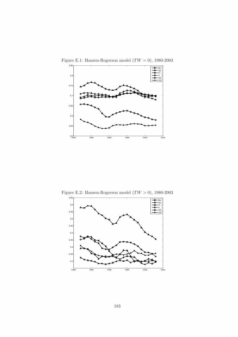
Figure E.1: Hansen-Rogerson model (TW = 0), 1980-2003
1980 1985 1990 1995 2000 20050.5
0.55
0.6
0.65
0.7
0.75
0.8
0.85
BeSpFrItUKUS
Figure E.2: Hansen-Rogerson model (TW > 0), 1980-2003
1980 1985 1990 1995 2000 2005
0.2
0.25
0.3
0.35
0.4
0.45
0.5
0.55
0.6
0.65
BeSpFrItUKUS
183

Essais sur les fluctuations economiques, la croissance et la performance du marche
du travail: l’impact de l’Etat providence
Cette these s’interesse aux fluctuations economiques, au chomage et a la croissance economique. Ces
dernieres decennies, la plupart des pays europeens ont connu un ralentissement de leur croissance economique
ainsi qu’un taux de chomage eleve et persistant. Cette evolution, dite de long terme, a ete accom-
pagnee d’une serie de fluctuations economiques de court terme. Dans ce contexte, cette these analyse
le fonctionnement du marche du travail et son incidence sur la performance des economies developpees.
Plus precisement, nous analysons les effets de court et de long terme de certaines distorsions jugees
representatives du marche du travail des pays europeens, tels que la fiscalite, les systemes d’indemnisation
du chomage et les mecanismes de fixation du salaire.
Le premier chapitre presente le modele canonique de cycle reel dans un contexte international. Il s’agit de
determiner un ensemble d’hypotheses visant a pallier aux defaillances du modele original dans l’explication
des fluctuations du marche du travail. L’incorporation de ces hypotheses dans ce cadre theorique fait
l’objet de la premiere partie du chapitre 2. Meme si ces amendements du cadre canonique conduisent a
une meilleure comprehension des determinants des fluctuations economiques et de leur synchronisation
entre pays, les faits concernant la dynamique des heures et du salaire ne sont pas expliques. Ceci justifie
le developpement d’une modelisation alternative du marche du travail, presente dans la deuxieme partie
de ce chapitre. Au centre de ce modele prennent place le chomage et les liens economiques entre pays.
Ce cadre est etendu au chapitre 3 pour integrer la fiscalite, ce qui nous permet de rendre compte de la
plupart des faits de court terme. Finalement, les chapitres 4 et 5 s’interessent a la problematique liee a
la croissance economique ainsi qu’a l’evolution tendancielle du temps du travail d’equilibre. En tenant
compte des rigidites presentes sur le marche du travail, nous fournissons une explication des phenomenes
de long terme.
Discipline: Sciences Economiques.
Mots cles: Fluctuations internationales, marche du travail, croissance, chomage, taxes et in-
stitutions du marche du travail.
Groupe d’Analyse des Itineraires et Niveaux Salariaux (GAINS-TEPP FR CNRS:
3126), Universite du Maine - Avenue Olivier Messiaen, 72085 Le Mans Cedex 9,
France.
184