Fluctuations. Introducing a

Leisure/Labor Choice in the Ramsey

Model. RBC models.

Olivier Blanchard∗

April 2005

∗ 14.452. Spring 2005. Topic 3. Figures at the end.

1

The benchmark model had shocks, uncertainty, but no variation in em-ployment. We want to explore what happens if we allow for a leisure/laborchoice.

This class of models is known as the RBC model. It does well at explain-ing many business cycle facts. Procyclical consumption, investment, andemployment.

But the hypotheses appear factually wrong (technological shocks, labor/leisureelasticity). Useless? No. Another step on the path to the relevant model.

Organization:

• Set up and solve the model. First order conditions, special cases, andnumerical simulations.

• Evidence on technological shocks, and the nature and the dynamiceffects of technological progress.

• Evidence on movements in non employment: Unemployment versusnon participation.

1 The optimization problem

Again look at a planning problem.

maxE[∞∑

0

βi U(Ct+i, Lt+i)|Ωt]

subject to:

Nt+i + Lt+i = 1

Ct+i + St+i = Zt+iF (Kt+i, Nt+i)

Kt+i+1 = (1− δ)Kt+i + St+i

2

The change from the benchmark: L is leisure and N is work. By normaliza-tion, total time is equal to one. Utility is a function of both consumptionand leisure.

Again I ignore growth. If growth, then the production function wouldhave Harrod neutral technological progress , so ZtF (Kt, AtNt), with At =At, A > 1 for example.

2 The first order conditions

The easiest way to derive them is again using Lagrange multipliers. Putthe three constraints together to get:

Kt+i+1 = (1− δ)Kt+i + Zt+iF (Kt+i, 1− Lt+i)− Ct+i

Associate βiλt+i with the constraint at time t:

E[U(Ct, Lt) + βU(Ct+1, Lt+1)− λt(Kt+1 − (1− δ)Kt − ZtF (Kt, 1− Lt) +Ct)− βλt+1(Kt+2− (1− δ)Kt+1−Zt+1F (Kt+1, 1−Lt+1) + Ct+1) + ... | Ωt]

The first order conditions are therefore given by:

Ct : UC(Ct, Lt) = λt

Lt : UL(Ct, Lt) = λtZtFN (Kt, 1− Lt)

Kt+1 : λt = E[βλt+1(1− δ + Zt+1FK(Kt+1, 1− Lt+1) | Ωt]

Define, as before, Rt+1 ≡ 1− δ + Zt+1FK(Kt+1, 1−Lt+1) and define Wt =ZtFN (Kt, 1− Lt), so:

3

UC(Ct, Lt) = λt

UL(Ct, Lt) = λtWt

λt = E[βλt+1Rt+1 | Ωt]

Interpretation (Optimization problem, consumers in the decentralized econ-omy, taking the wage and the interest rate as given). Combining the firsttwo:

The intratemporal condition:

UL(Ct, Lt) = WtUC(Ct, Lt)

And the intertemporal condition:

UC(Ct, Lt) = E[βRt+1UC(Ct+1, Lt+1) | Ωt]

Before proceeding, we can ask: What restrictions do we want to impose on

utility and production so as to have a balanced path in steady state?

(Not a totally convincing exercise:

There is actually a fairly strong downward trend in hours worked (see figure

at the end of hand out on hours worked over time for major countries), so

not clear that we are on a balanced growth path.

Even if we were, do we really have the same preferences in the short and

the long run? Could have all kinds of dynamic specifications of utility with

the same implications for the long run.)

4

• On the production side, we know that progress has to be Harrod

Neutral, say at rate A > 1. (Remember we suppressed At just for

notational convenience.

• On the utility side, can use the first order conditions above to derive

the restrictions.

In steady state, leisure is constant. Consumption and the wage increase at

rate A, so, from the intratemporal condition:

UL(CAt, L)UC(CAt, L)

= WAt

where C, L and W are constant over time, and A increases. This is true

for any At, so in particular, for t = 0 so At = 1, so

UL(C,L)UC(C, L)

= W

Using the two relations to eliminate the wage, we can write:

UL(CAt, L)UC(CAt, L)

= At UL(C,L)UC(C,L)

The marginal rate of substitution between consumption and leisure must

increase over time at rate A.

This relation holds for any value of the term At So use for example At =1/C:

UL(1, L)UC(1, L)

=1C

UL(C, L)UC(C, L)

Or, rearranging:

5

UL(C,L)UC(C,L)

= C[UL(1, L)UC(1, L)

]

The rate of substitution must be equal to C times the term in brackets,

which is a function only of L. This in turn implies that the utility function

must be of the form:

u(Cv(L))

Now turn to the intertemporal condition. Write it as:

UC(CAt, L) = (βR)UC(CAt+1, L)

Or, given the restrictions above:

u′(CAtv(L))u′(CAt+1v(L))

= βR

For this condition to be satisfied, u(.) must be of the constant elasticity

form:

u(Cv(L)) =σ

σ − 1(Cv(L))(σ−1)/σ

If σ = 1, then:

U(C, L) = log(C) + v(L)

where v(L) = log(v(L)), with v′ > 0, v′′ < 0. (Another way of stating this.

If we want to assume separability of leisure and consumption (but there

is really no good reason to do that), then the form above is the only one

consistent with the existence of a steady state.

6

Let me use the specification U(C,L) = log(C) + v(L) and return to thefirst order conditions.

The intratemporal condition becomes:

v′(Lt) = Wt/Ct

And the intertemporal condition:

E[βRt+1Ct

Ct+1| Ωt] = 1

Interpretation. (Note that UC = 1/C is the marginal value of wealth). Soequalize marginal utility of leisure to the wage times the marginal value ofwealth. And the Ramsey-Keynes condition for consumption.

So now consider the effects of a favorable technological shock. It increasesW and R, both current and prospective.

• Two effects on consumption. Smoothing (consumption up) and tilt-ing (consumption down). On net, plausibly up.

• Turn to leisure/work. Two effects.A substitution effect: Higher Wt leads people to work harder.An income/wealth effect. Higher Ct works the other way. As peoplefeel richer (remember that 1/C is the marginal value of wealth), theywant to consume more and enjoy more leisure.Net effect depends on the strength of the two effects. Substitution(elasticity), and wealth (persistence).

• The more transitory the shock, the smaller the increase in C, and sothe stronger the substitution effect.

• The more permanent (with Ct increasing as much or more than Wt.Can it? Yes. Think of a permanent shock, plus capital accumulation),the stronger the wealth effect. Employment could decrease.

7

Another way of looking at the employment effects. An intertemporal con-dition for leisure (this is the way Lucas and Rapping looked at it):

Replace consumption by its expression from the intratemporal condition.And, just for convenience, use v(L) = φ log(L), so v′(L) = φ/L. Then:

φCt = WtLt

So, replacing in the intertemporal condition:

E[β(Rt+1Wt

Wt+1)

Lt

Lt+1| Ωt] = 1

What is relevant for the leisure decision is the rate of return “in wageunits”.

Now consider a transitory shock, so Wt increases but Wt+1 does not changemuch. Then Lt/Lt+1 will decrease sharply. The increase in the wage willbe associated with a strong increase in employment.

Consider a permanent shock: Then Wt/Wt+1 is roughly constant, and sois Lt/Lt+1. (ignoring movements in R). No movement in employment.

3 Solving the model.

The usual battery of methods:

Special cases? The same as before. Assume Cobb Douglas production,assume log–log utility. Assume full depreciation.

Kt+1 = ZtKαt (1− Lt)

1−α − Ct

8

and

U(Ct, Lt) = log Ct + φ log Lt

Then, can solve explicitly. And the solution actually is identical to that ofthe benchmark model. N is always constant, not by assumption, but byimplication now. Substitution and income effects cancel.

Ct = (1− αβ)Yt

N | φ

1−N=

1− α

1− αβ

1N

So, nice, but not useful if we want to think about fluctuations in employ-ment.

So need to go to numerical simulations. SDP, or log linearization. Camp-bell gives a full analytical characterization. On the web page, you canfind a Matlab program written by Thomas Philippon and Ruben Segura-Cayuela for the log linearized model (with Cobb Douglas production andlog-log preferences). (“RBC.m” and associated programs give the impulseresponses, and the moments, and correlations of the variables with output.Play with it).

The effects of different persistence parameters for the technological shocks.See figures from RBC.m for three values of ρ. Could do the same for differ-ent elasticities of labor supply, or different intertemporal elasticities. Butin these two cases, you need to modify the matrices a bit. You may wantto do it.

(See also results from King Rebello. Tables 1, 3. And their figure 7.)

9

Success? Not yet:

• Labor supply elasticities: plausible?• Technological shocks. Are they really there?

4 Movements in employment and the labor/leisure choice

Within the logic of the model: Under the log-log assumption used by Kingand Rebello and others, the elasticity of employment with respect to thewage, controlling for consumption (so as to eliminate the income/wealtheffect) is given by:

dN

N= −dL

L

1−N

N=

1−N

N

dw

w

So, if we assume, like King-Rebello, that N = .2 (that we spend 20% ofour time working), then the elasticity of employment with respect to thewage is 4.

Empirical estimates (of which there are many in the micro-labor lit) areall much lower, below 1. If we assume an elasticity of 1 in the RBC model,then, as shown in Figure 8 of King-Rebello, we do not get much action inemployment relative to the data.

Is this deadly? Not necessarily. It suggests that the competitive spot marketcharacterization of the labor market has to be replaced by something else.

This is the approach which has been explored by the “flows and bargaining”line of research. This approach thinks of and formalizes the labor marketas a market characterized by flows of workers in and out of jobs, and ofwages being set by bargaining between firms and workers. You will see itin detail in 454.

10

In this approach, the causal relation between wages and employment runsfrom employment (or unemployment, or in general, any variable character-izing the state of the labor market) to (bargained) wages: How much does achange in employment (unemployment) affect bargained wages? (Contrastthis with the competitive labor market formalization in the RBC modelabove, where the causal relation runs from wages to employment: Howmuch do wages affect employment (labor supply)?)

And the question becomes: Do we have a convincing explanation for whychanges in employment lead to a small response of wages? This is thesubject of much current research. The answer is not yet in.

But the answer is central, not only for RBC models, but, as we shall see,in New Keynesian models. All these models generate plausible responsesof the economy to shocks only if the elasticity of wages to employment issmall (equivalently, if the elasticity of employment to wages is high).

5 Technological shocks. Evidence

A priori, the notion that there would be sharp movements in the productionfrontier from quarter to quarter, highly correlated across sectors, is notplausible. The diffusion of technology is steady. Breakthroughs are rare,and unlikely to be in all sectors at once.

(Exceptions:

For example, a breakdown in the rule of law. Then, suddenly, many rela-tions come to an end, and the effective production frontier shrinks. Relevantfor example in Eastern Europe in the early 1990s

And relevant at slightly lower frequencies. Clear that technological shocks(the high tech boom) had something to do with the expansion of the sec-ond half of the 1990s, and the subsequent recession. Perhaps not howeverthrough the RBC channels).

11

So second look:

5.1 The measurement of technological shocks

One way to measure technological progress was suggested by Solow. Theconstruction of the Solow residual goes like this:

Suppose the production function is of the form:

Y = F (K,N,A)

A is the index of technological level, and enters the production functionwithout restrictions. We want to measure the contribution of A to Y .

Differentiate and rearrange to get:

dY

Y=

FKK

Y

dK

K+

FNN

Y

dN

N+

FAA

Y

dA

A

Suppose now that firms price according to marginal cost. Let W be the priceof labor services, and R be the rental price of capital services. Assume nocosts of adjustment for either labor or capital. Then:

P = MC = W/FN = R/FK

Replacing:

dY

Y=

RK

PY

dK

K+

WN

PY

dN

N+

FAA

Y

dA

A

Define the Solow residual as S ≡ (FAA/Y )(dA/A). Let αK be the shareof capital costs in output, and αN be the share of labor costs in output.Then:

12

S =dY

Y− dX

X

where

dX

X≡ αK

dK

K+ αN

dN

N

The Solow residual is equal to output growth minus weighted input growth,where the weights are shares (and time varying). No need for estimation,or to know anything about the production function.

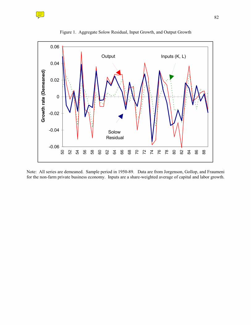
If we construct the residual in this way:

• Get a highly procyclical Solow residual. Figure 1 from Basu.• Get a very good fit with output: From annual data from 1960 to 1998

(different time period from Basu graph):

dY

Y= 1.16 S + 0.36 S(−1) + ε R2 = .82

Solow used this approach to compute S over long periods of time. Is itreasonable to construct it to estimate technological change from year toyear, or quarter to quarter? The answer is: Probably not.

A number of serious problems. Among them:

• Costs of adjustment. If costs of adjustment to capital, then the shadowrental cost is higher/lower than the rental price R. Same if costs ofadjustment to labor. So shares using rental prices or wages may notbe right.

• Non marginal cost pricing. Firms may have monopoly power, in whichcase, markup µ will be different from one.

• Unobserved movements in N or K. Effort? Capacity utilization?

Examine the effects of the last two (On costs of adjustment just to capital,no problem. Condition still holds for labor, so use the share of labor to

13

weight the change in employment. And use one minus the share of laborto weight the change in capital. More of an issue if costs of adjustment toboth.)

Markup pricing

Suppose

P = (1 + µ) MC

Then: P = (1+µ)W/FN or FN = (1+µ)W/P . Similarly FK = (1+µ)R/P .So:

S =dY

Y− (1 + µ)

dX

X

Let the measured Solow residual be S, and true Solow residual be S. Then,if µ > 0 and we construct the Solow residual in the standard way, then weshall overestimate the Solow residual when output growth/input growth ishigh. :

S = S − µdX

X

Figure, for µ = 0.1, 0.2, from Basu. Adjusted Solow Residual much lessprocyclical. But have to go to high values of µ, say 0.5 to eliminate pro-cyclicality.

Unobserved inputs

Suppose for example that N = BHE, where B is number of workers, H ishours per worker, and E is effort. Going through the same steps as before,leaving markup pricing aside:

14

S ≡ dY

Y− [αK

dK

K+ αN (

dB

B+

dH

H+

dE

E)]

Suppose we observe B and H but not E, so measure labor (incorrectly)by BH. Then, again, we shall tend to overestimate the Solow residual inbooms:

S = S − αNdE

E

Similar issues with capacity utilization on the capital side.

Are there ways around it?

Suppose that we allow for markup pricing and unobserved effort. Then:

S =dY

Y− (1 + µ)

dX

X− (1 + µ)αN

dE

E

Or, equivalently:

dY

Y= (1 + µ)

dX

X+ (1 + µ)αN

dE

E+ S

Can we estimate it and get a series for the residual? There are two problems:

• Unobservable effort dE/E ? Part of the error term, likely to be cor-related with dX/X.If firms cost minimize at all margins and can freely adjust effort andhours, then, under reasonable assumptions, dE/E and dH/H willmove together. So will capacity utilization. So can estimate:

dY

Y= (1 + µ)

dX

X+ βαN

dH

H+ S

15

• S correlated with dX/X? Likely as well. Surely under RBC hypothe-ses. So, need to use instruments: Government spending on defense, oilprice, federal funds innovation... Good instruments? Might be easierin a small economy: World GDP.

Results. Basu and Fernald. Find markup around 1, so that correction makeslittle difference. But the correction for hours makes the estimated Solowresidual nearly a-cyclical. See their Figure 3.

Role of technological shocks? Variance decomposition of a bivariate VARin the estimated residual and the usual Solow residual:

Contribution of technological shock to Solow residual, 5% on impact, 38%after a year, 59% after 3 years, 66% after 10 years.

Having constructed an adjusted series, can look at the dynamic effects onoutput, employment, and so on. This is done by Basu, Fernald, and Kimball(NBER WP 10592)

5.2 An alternative way of identifying technological shocks

An alternative construction of shocks, and the results. Gali 2004, expandingon Blanchard Quah, 1989.

Identify the technological shocks as those shocks with a long term effect onproductivity, and then trace their short run effects on output, employment,productivity.

Technically:

• Estimate a bivariate VAR in ∆ log(Y/N) and ∆ log(N). Station-ary. So no effect of shocks on productivity growth and employmentgrowth. But potential effects on level of productivity, and level ofemployment.

16

• Assume two types of shocks. Shocks with permanent effects on levelof productivity. Shocks with no permanent effects on level of produc-tivity. This is sufficient for identification.

• Call the first “technological shocks.” Impulse responses (get the im-pulse responses for productivity growth and employment growth.Easy to then get impulse responses for output, employment and pro-ductivity levels (how?) . Figure 2 in Gali.Find an increase in output, but less than productivity. So a (small)decrease in employment (measured by total hours worked).By constructing the movements in Y due to the technological shocks,can see how much of the cyclical movements in Y are explained bythese shocks. This is done in Figure 3 in Gali. The answer: not much.(An alternative measure would be to show variance decompositionsat various forecast horizons.)

• Blanchard Quah differs in the two variables looked at: log output,and unemployment rate. Less appealing: output may be affected bymore than technological shocks in the long run.Impulse responses: technological shocks on output build up slowly.Variance decomposition: Tables 2 to 2B. Due to technological shocks:1% to 16% at one quarter, 20 to 50% at 8 quarters.

• How robust? My reading: fairly robust. See discussion in Gali. (Aswas pointed out in the lecture, earlier Gali 1992 (problem set 1) findsa larger role for technological shocks at cyclical frequencies).

• An independent confirmation. Basu et al (2004) trace the effects oftheir constructed measure of technological shocks on output, employ-ment. They find an initially negative effect of the shocks on employ-ment.

5.3 Technological progress and fluctuations

Other relevant papers/approaches. In no particularly tight order.

17

• One reason for doubting the existence of large aggregate technologicalshocks is the law of large numbers. Technological shocks may be largein the short run in one firm, perhaps one sector, but likely to washout for the economy as a whole.This is questioned by Gabaix (on the reading list) who argues, the-oretically and empirically, that idiosyncratic shocks may be largeenough to explain a good part of aggregate fluctuations (so the lawof large numbers fails).

• Along related lines, one would expect to see potentially large tech-nological shocks at the firm or sectoral level, but largely washing outin the aggregate.Franco and Philippon (not on the reading list, “Firms and aggre-gate dynamics”, http://ssrn.com/abstract=640584), look at a panelof firm, allowing firms to be affected by permanent shocks to technol-ogy, permanent shocks to relative demand, and common aggregate(demand?) shocks. They find a large role for permanent shocks totechnology at the firm level, largely washing out in the aggregate.

• Sector specific innovations are unlikely to show up as large move-ments in the economy’s production frontier from year to year. Theyare likely to be implemented over time, and to be largely uncorrelatedover time.Some technological changes however can shift the production frontierin many sectors. These are known as general purpose technologies,and run from electricity to computers. They are likely to diffuse overtime to many sectors. This appears to have been for example the casein the second half of the 1990s in the United States.During that time, there appears to have an increase in tfp growth inIT producing sectors, and an increase in both capital intensity andtfp growth in the other (IT using) sectors. The decrease in capitalintensity is plausibly attributed to the decrease in the price of IT

18

capital goods. The (small) increase in tfp growth in the IT usingsectors is plausibly attributed to changes in organization facilitatedby the installation of IT capital. (See Jorgenson and Stiroh article onRL).Such periods are likely to be characterized by higher growth for sometime. (During those periods, consumption and investment demandmay also boom, leading to an increase in aggregate demand whichleads to even more output growth than warranted by the increase intfp on the supply side. This is for example Greenspan’s interpretationof that half decade).

• Another hypothesis is that the introduction of GPTs may be associ-ated with lower measured tfp growth for some time.Initially, the introduction of new technologies may require firms toreorganize, or put another to invest in organization capital. Duringthat time, measured output may well decline. (When we learn to usea new program, our measured productivity goes down).This could provide an explanation for Solow’s paradox, the remarkin the early 1990s that computers could be seen everywhere exceptin productivity statistics. Under that explanation, lower productiv-ity growth in the 1980s and early 1990s reflected investment andlearning. We are now seeing the positive effects in the form of highermeasured tfp growth. (See work by Greenwood)The hypothesis is appealing, and surely relevant in many cases at themicro level. Whether it can explain the slowdown in tfp growth afterthe mid 1970s remains an open issue. It does not seem to have muchto say about recessions.

• Reverse causality: Fluctuations due to other shocks are likely to havesome lasting effects on total factor productivity.On the one hand, recessions are likely to lead to the closing of theleast productive firms. In this sense, recessions may “cleanse” the

19

economy, leading to higher productivity, at least for some time.On the other, in the presence of imperfections in credit markets,recessions may lead to inefficient cleansing, the closing of efficient,but credit constrained firms. (see work by Ricardo Caballero)Which way it goes appears empirically ambiguous. There is some(but only mildly convincing) evidence that recessions due to nontechnological shocks are followed by permanently higher productivity.

• One hypothesis, explored by Lilien in the 1980s, is that variationsin unemployment may be due to higher reallocation across firms,coming from a higher pace on technological progress. In that case,higher technological progress could be associated with higher unem-ployment.The empirical evidence does not support this view. Under that view,one would expect fluctuations to be associated with positive co move-ments between unemployment (workers looking for jobs) and vacan-cies (jobs looking for workers). Exactly the opposite holds. Fluctua-tions are associated with opposite movements in vacancies and un-employment. (This negative relation between vacancies and unem-ployment is known as the Beveridge curve).

• An attractive story for why technological progress might lead to cy-cles was developed by Shleifer (see RL).Suppose the rate of innovation is constant, but firms can decide aboutthe timing of implementation of their innovation. Suppose that firmsget rents from the introduction of a new product, but these rentsdisappear over time due to entry of competitors.Then firms will want to introduce their products when rents arelargest, thus when aggregate demand is highest. Aggregate demandwill be highest when many firms introduce their products, leading toan increase in aggregate income. Thus, the economy will exhibit im-plementation cycles, times when many firms introduce new products,

20

followed by quiet times, and a new burst of implementation.How relevant? It appears to fit aspects of the 1990s. It provides per-haps the most plausible account of why smooth discoveries may leadto sharper aggregate cycles.

21

17

Figure 1 Annual Hours Worked Over Time

OECD data. Annual hours per employed person. Annual hours are equivalent to 52*usual weekly hours minus holidays, vacations, sick leave.

1000

1200

1400

1600

1800

2000

2200

1960

1962

1964

1966

1968

1970

1972

1974

1976

1978

1980

1982

1984

1986

1988

1990

1992

1994

1996

1998

2000

2002

US

Germany

France

Italy

0 5 10 15 20 25 30 35 40-0.2

0

0.2

0.4

0.6

0.8

1

1.2

1.4

1.6Impulse responses to a shock in technology

Quarters, rho=.974

Perc

ent d

evia

tion

from

ste

ady

stat

e

technology capital

output

consumption

interest rate

employment

real wage

0 5 10 15 20 25 30 35 40-0.2

0

0.2

0.4

0.6

0.8

1

1.2

1.4

1.6Impulse responses to a shock in technology

Quarters, rho=.999

Perc

ent d

evia

tion

from

ste

ady

stat

e

technology

capital

output

consumption

interest rate

employment

real wage

0 5 10 15 20 25 30 35 40-0.2

0

0.2

0.4

0.6

0.8

1

1.2

1.4

1.6

1.8Impulse responses to a shock in technology

Quarters, rho=.9

Perc

ent d

evia

tion

from

ste

ady

stat

e

technology

capital output

consumption

interest rate

employment

real wage

Lu fb At tih@* ULhhi*@|L? t |i hi@tL? ) |ihi t tL4i Thi_U|@M*|)|L |i Mt?itt U)U*i

A@M*i t?itt )U*i 5|@|t|Ut uLh |i N5 ,UL?L4)

5|@?_@h_#i@|L?

+i*@|i5|@?_@h_#i@|L?

6ht|h_ih|LULhhi*@|L?

L?|i4TLh@?iLtLhhi*@|L?||T|

v H ff fHe ff D f.e fHf fHHW Df 2b fH. fHf .b fbb fHH fHHv% f2 fDS f.e fDD fSH fH fSS f2h ff fS fSf fD fbH fDe f.e f.H

L|iG ** @h@M*it @hi ? *L@h|4t E| |i i UiT|L? Lu |ihi@* ?|ihit| h@|i @?_ @i Mii? _i|hi?_i_ | |i O *|ih #@|@tLhUit @hi _itUhMi_ ? 5|LU! @?_ @|tL? dbbHoc L Uhi@|i_ |ihi@* h@|i t? V+ ?@|L? i TiU|@|L?t h ?L|@|L? ? |t |@M*iULhhitTL?_t |L |@| ? |i |i |c tL |@| v t Tih U@T|@ L|T|c t TihU@T|@ UL?t4T|L?c W t Tih U@T|@ ?it|4i?|c t Tih U@T|@ Lhtc t |i hi@* @i EUL4Ti?t@|L? Tih Lhc h t |i hi@* ?|ihit| h@|ic@?_ t |L|@* u@U|Lh ThL_U||)

W? Thiti?|? |iti Mt?itt U)U*i u@U|tc i @hi uLUt? L? @ t4@** ?4MihLu i4ThU@* ui@|hit |@| @i Mii? i |i?ti*) _tUtti_ ? hiUi?| Lh! L? hi@*Mt?itt U)U*it 6Lh i @4T*ic ? |i ?|ihit| Lu Mhi|)c i @i ?L| _tUtti_ |i*i@_*@ hi*@|L?t Mi|ii? Lh @h@M*it W? ULLt? |i tihit |L t|_)c i @i@*tL *iu| L| ?L4?@* @h@M*itc Lti U)U*U@* Mi@Lh t @| |i i@h| Lu 4@?)UL?|hLihtit Lih |i ?@|hi Lu Mt?itt U)U*it OLiihc i _L hiTLh| |i

46Vhh Vwrfn dqg Zdwvrq ^4<<;/ vhfwlrqv 6+g,/ 6+i,/ dqg 714` iru d glvfxvvlrq ri olwhudwxuh dqghpslulfdo uhvxowv1

b

hiTLh|i_ ? |i tiUL?_ UL*4?t Lu A@M*it @?_ W? T@h|U*@hc ?it|4i?| t@ML| |hii |4it 4Lhi L*@|*i |@? L|T| ? ML| |i @U|@* iUL?L4) Eihi|i h@|L Lu t|@?_@h_ _i@|L?t t Df%H'2b @?_ |i 4L_i* iUL?L4) Eihi|i h@|L Lu t|@?_@h_ _i@|L?t t 2bD L?t4T|L? t tMt|@?|@**) t4LL|ih|@? L|T| ? ML| |i 4L_i* @?_ @U|@* iUL?L4it W? Lh M@tU 4L_i*c LiihcUL?t4T|L? t L?*) @ML| L?i|h_ @t L*@|*i @t L|T| *i | t Lih |L |h_t@t L*@|*i @t L|T| ? |i N5 iUL?L4) i hi|h? |L _tUttL? Lu |t ui@|hiLu |i iUL?L4) ? tiU|L? S Mi*L

A@M*i t?itt )U*i 5|@|t|Ut uLh @tU + L_i*D

5|@?_@h_#i@|L?

+i*@|i5|@?_@h_#i@|L?

6ht|h_ih|LULhhi*@|L?

L?|i4TLh@?iLtLhhi*@|L?||T|

v b ff f.2 ff fS fee f.b fbeW efb 2bD f. fbb fS. feH f. fb.v% f.D fDe f.S fbH f.D fDe f.S fbHh ffD ffe f. fbD fbe fSH f.2 ff

L|iG ** @h@M*it @i Mii? *Li_ E| |i i UiT|L? Lu |i hi@*?|ihit| h@|i@?_ _i|hi?_i_ | |i O *|ih

ihtt|i?Ui @?_ UL4Li4i?| | L|T| t?itt U)U*it @hi Tihtt|i?|*) Lh *L *ii*t Lu iUL?L4U @U||)G L?i 4i@thi Lu |t Tihtt|i?Ui t |i ht|Lh_ihtih@* ULhhi*@|L? ULiUi?| A@M*i tLt |@| |i Tihtt|i?Ui i?ih@|i_ M) |iM@tU 4L_i* t i?ih@**) c M| i@!ih |@? ? |i _@|@ Etii A@M*i Aihi*@|i t|@?_@h_ _i@|L?t @*tL ThL_i @ 4i@thi Lu |i *4|i_ i |i?| |L U

68Wkh prphqwv lq wklv wdeoh duh srsxodwlrq prphqwv frpsxwhg iurp wkh vroxwlrq ri wkh prgho1Suhvfrww ^4<;9` surgxfhg pxowlsoh vlpxodwlrqv/ hdfk zlwk wkh vdph qxpehu ri revhuydwlrqv dydlo0deoh lq wkh gdwd/ dqg uhsruwhg wkh dyhudjh KS0owhuhg prphqwv dfurvv wkhvh vlpxodwlrqv1

2b

)LJXUH :

2XWSXW

0;

09

07

05

3

5

7

9

84 89 94 99 :4 :9 ;4 ;9 <4 <9

'DWH

3HUFHQW

0RGHO'DWD

/DERU ,QSXW

0;

09

07

05

3

5

7

84 89 94 99 :4 :9 ;4 ;9 <4 <9

'DWH

3HUFHQW

0RGHO'DWD

,QYHVWPHQW

058

053

048

043

08

3

8

43

48

53

84 89 94 99 :4 :9 ;4 ;9 <4 <9

'DWH

3HUFHQW

0RGHO'DWD

&RQVXPSWLRQ

07

06

05

04

3

4

5

6

7

8

9

84 89 94 99 :4 :9 ;4 ;9 <4 <9

'DWH

3HUFHQW

0RGHO'DWD

1RWH= 6DPSOH SHULRG LV 4<7:=5 0 4<<9=71 $OO YDULDEOHV DUH GHWUHQGHG XVLQJ WKH +RGULFN03UHVFRWW ILOWHU1

)LJXUH ;

2XWSXW ZLWK VPDOO $ VKRFNV

0;

09

07

05

3

5

7

9

84 89 94 99 :4 :9 ;4 ;9 <4 <9

'DWH

3HUFHQW

0RGHO'DWD

/DERU ,QSXW ZLWK VPDOO $ VKRFNV

0;

09

07

05

3

5

7

84 89 94 99 :4 :9 ;4 ;9 <4 <9

'DWH

3HUFHQW

0RGHO'DWD

2XWSXW ZLWK VPDOOHU ODERU HODVWLFLW\

0;

09

07

05

3

5

7

9

84 89 94 99 :4 :9 ;4 ;9 <4 <9

'DWH

3HUFHQW

0RGHO'DWD

/DERU ,QSXW ZLWK VPDOOHU ODERU HODVWLFLW\

0;

09

07

05

3

5

7

84 89 94 99 :4 :9 ;4 ;9 <4 <9

'DWH

3HUFHQW

0RGHO'DWD

1RWH= 6DPSOH SHULRG LV 4<7:=5 0 4<<9=71 $OO YDULDEOHV DUH GHWUHQGHG XVLQJ WKH +RGULFN03UHVFRWW ILOWHU1

7A

5< + *-&9+*E&9+

'< & & 56D@/76; *9&*

/& -& /+ &+

7J

F$ *+ *E&-&9+

'$ /" *+

(" ,) / < & /

+ &+< &

& 56D@/76

Figure 2. The Estimated Effects of Technology ShocksDifference Specification , 1948:01-2002:04

Productivity: Dynamic Response

0 2 4 6 8 10 120.45

0.54

0.63

0.72

0.81

0.90

0.99

1.08Productivity: Impact Response

0.56 0.63 0.70 0.77 0.84 0.910

1

2

3

4

5

6

7

Output: Dynamic Response

0 2 4 6 8 10 12-0.25

0.00

0.25

0.50

0.75

1.00

1.25

1.50Output: Impact Response

0.00 0.24 0.48 0.720.0

0.5

1.0

1.5

2.0

2.5

3.0

Hours: Dynamic Response

0 2 4 6 8 10 12-0.8

-0.6

-0.4

-0.2

-0.0

0.2

0.4

0.6Hours: Impact Response

-0.5000000 -0.20000000

1

2

3

4

5

Figure 3: Sources of U.S. Business Cycle FluctuationsDifference Specification , Sample Period:1948:01-2002:04

Technology-Driven Fluctuations (BP-filtered)

1948 1952 1956 1960 1964 1968 1972 1976 1980 1984 1988 1992 1996 2000-5.4

-3.6

-1.8

-0.0

1.8

3.6

5.4

y n

Other Sources of Fluctuations (BP-filtered)

1948 1952 1956 1960 1964 1968 1972 1976 1980 1984 1988 1992 1996 2000-5.4

-3.6

-1.8

-0.0

1.8

3.6

5.4

Figure 5. Technology Shocks: VAR vs. BFK

VAR Permanent Shocks vs. BFK

1950 1953 1956 1959 1962 1965 1968 1971 1974 1977 1980 1983 1986 1989-2.5

-2.0

-1.5

-1.0

-0.5

0.0

0.5

1.0

1.5

2.0

VAR BFK

VAR Transitory Shocks vs. BFK

1950 1953 1956 1959 1962 1965 1968 1971 1974 1977 1980 1983 1986 1989-2.4

-1.6

-0.8

-0.0

0.8

1.6

2.4