"STRATEGIC MARKETING, PRODUCTION,AND DISTRIBUTION PLANNING OF AN

INTEGRATED MANUFACTURING SYSTEM

by

Luk VAN WASSENHOVE*Jalal ASHAYERI**

andBehnam POURBABAI***

N° 92/47/TM

* Professor of Operations Management and Operations Research, at INSEAD, Boulevard deConstance, Fontainebleau 77305 Cedex, France.

** Professor at Tilburg University, 5000 LE Tilburg, The Netherlands.

*** Professor at The University of Maryland, College Park, MD 20742, U.S.A.

Printed at INSEAD,Fontainebleau, France

Strategic Marketing, Production, and Distribution Planning of anIntegrated Manufacturing System

Behnam PourbabaiDepartment of Mechanical Engineering

The University of MarylandCollege Park, MD 20742, USA.

Jalal AshayeriDepartment of Econometrics

Tilburg University5000 LE Tilburg, The Netherlands

Luk Van WassenhoveTechnology Management Area

INSEAD, Boulevard de ConstanceFontainebleau 77305 Cedex, France

ABSTRACT

This paper extends Pourbabai's (1991) results for generating a strategic marketing andproduction plan for an Integrated Manufacturing System (IMS) to include distribution decisions.The paper introduces additional distribution decision variables and constraints for both ofloading models proposed by Pourbabai (1991). The new models optimize the utilization of theprocessing capabilities of an IMS consisting of a set of heterogeneous workstations. Theobjective to be maximized includes, the fixed and variable market values of each job, the fixedand variable processing costs of each job, the setup costs, and the fixed and variable distributioncosts. Each job requires a single aggregated stage of operation; job splitting is allowed; and theprocessing priorities of all jobs during the planning time horizon are given. Setup timescollapsing is also allowed, to shorten the completion times of some jobs. The proposed modelsare fixed charge problems which can be solved by a mixed integer programming algorithm.

Key Words: Loading Strategy, Aggregate Scheduling, Aggregate Production and DistributionPlanning, Decision Support System, Optimization.

1. INTRODUCTION

Computer Integrated Manufacturing (CIM) concepts such as CAD, CAM, Group Technology

(GT), etc. are implemented in many manufacturing industries. Many companies have improved

the entire supplier/ customer chain by sharing information through better communication systems

across the full spectrum of the supply chain and by implementing other CIM concepts. However,

the potential benefits of CIM have not yet been fully realized. One of the major requirements

for achieving full benefits is a general revision of the techniques of planning and control of

production and distribution. A careful planning of production and distribution is vital for an

efficient exploitation of production capabilities of Integrated Manufacturing Systems (IMS).

In this paper, quantitative decision making models developed by Pourbabai (1991) are extended

in order to include distribution decisions. This is necessary when workstations (production lines)

are in different locations, in order for the proposed models to properly tradeoff profit

components with various costs involved in production and distribution. Indeed, transportation

time introduces another constraint which needs to be considered in order to meet the due dates

set. In some cases the transportation time is far longer than the manufacturing throughput time.

Examples of this type of environment are car or hifi manufacturers who have several production

lines in different countries and produc their goods Just-In-Time. In such situations the costs and

the role of distribution cannot be neglected.

The new models include :

i) distribution costs such as short term holding costs and transportation costs fromworkstations to distribution centers and from distribution centers to customers;

ii) additional constraints to explicitly consider the transportation times from workstations todistribution centers and from distribution centers to customers.

The objective to be maximized models the tradeoffs between total sales income, total processing

costs, total distribution costs, and total setup costs of the supply chain. The new models can

assist operations managers in selecting potential customer orders such that the net operational

profit during the planning horizon will be maximized. Based on these models, the profitable

2

Strategic Marketing, Production,

and Distribution Model

List of Accepted Customer Orders

An Operational Loading Plan

Verify the Feasibility of the Operational

Plan by an Appropriate Performance

Evaluation Model

Feasible Operational Plan

List of theRejected

Cusromer orders

No

orders and the lot-sites of each component of each job at each workstation (production line) will

be identified. Furthermore, based on the solutions of these models, the resulting operational

plans can be plotted on Gantt charts for shop floor supervisors.

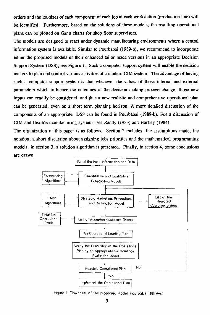
The models are designed to react under dynamic manufacturing environments where a central

information system is available. Similar to Pourbabai (1989-b), we recommend to incorporate

either the proposed models or their enhanced tailor made versions in an appropriate Decision

Support System (DSS), see Figure 1. Such a computer support system will enable the decision

makers to plan and control various activities of a modem CIM system. The advantage of having

such a computer support system is that whenever the values of those internai and external

parameters which influence the outcomes of the decision making process change, those new

inputs can readily be considered, and thus a new realistic and comprehensive operational plan

can be generated, even on a short term planning horizon. A more detailed discussion of the

components of an appropriate DSS can be found in Pourbabai (1989-b). For a discussion of

CIM and flexible manufacturing systems, see Randy (1983) and Hartley (1984).

The organization of this paper is as follows. Section 2 includes the assumptions made, the

notation, a short discussion about assigning jobs priorities and the mathematical programming

models. In section 3, a solution algorithm is presented. Finally, in section 4, some conclusions

are drawn.Read the Input Information and Data

Forecasting

Algorithms

MIP

Algorithms

Total NetOperational

Profit

Quantitative and Qualitative

Forecast ng Models

Yes

Implement the Operational Plan

Figure 1. Flowchart of the proposed Model, Pourbabai (1989-c)

3

2. MODEL COMPONENTS

2.a. Limitations and Capabilities

1. The planning horizon needs to be sufficiently short to enable decision makers toexplicitly or implicitly consider all changes due to the internai and external informationat the beginning of each planning horizon. Hence, new operational plans can begenerated as frequently as needed.

2. Workstations (production lines) are situated in different locations.

3. Based on the bill of materials, the following parameters should be identified;

i) the number of units of each component of each product. Note that a component maybe used in different products. In this paper, the term "job" refers to a batch of identicalparts;

ii) the due date of each job; and

iii) the release date of each job; i.e. the earliest time that a job can start.

4. Each workstation (production line) is designed based on the GT concept (see Waghodekarand Sahu (1983) and Ham et al. (1985)). Furthermore, all operations on a job areassumed to be executable on at least one of the workstations. Hence, we only require anestimate of the total required processing time for each job at each compatibleworkstation.

5. The required aggregated processing time at each workstation is a random variable andcould consist of the following corresponding time components (random variables):

i) summation of the processing times of all operations of each generic workpiecebelonging to the family of parts at the corresponding workstation;

ii) the routing delay time;

iii) the operator delay time;

iv) the machine loading delay time;

v) the machine unloading delay time;

4

vi) the breakdown times and the corresponding repair times;

vii) the material handling delay time.

Thus, the aggregated processing time is in effect the resulting convolution of a finitenumber of random variables (e.g., routing delay time, loading delay time, etc.). In ourmodels, only the expected value of the aggregated processing time at each workstationis used.

6. If there are jobs that can be processed at compatible workstations, job splitting is allowedfor each job. That is, each batch of identical parts can be split among all the compatibleworkstations which are individually capable of processing all operations. The primaryeffect of job splitting is to reduce the completion time of each job;

7. The processing order of the jobs is prespecified according to a desirable dispatching ruleduring the short term planning horizon (see section 2.c).

8. Setup times can sometimes be saved by combining batches of the same job types but withdifferent due dates.

2.b. Notations

Indices:

i : the job type index;(i=1,...,N)

j : the workstation (production line) index;(1 = 1,...,M)

k : the due date index (i.e. k=1 is the first order to bedelivered, k=2 the second order to be delivered andso on.);(k=1,...,K)

1 : the distribution center index;(1=1,...,L)

Parameters:

:= the job with job type index i of the customer with the due date index k whichhas to be produced at workstation j;

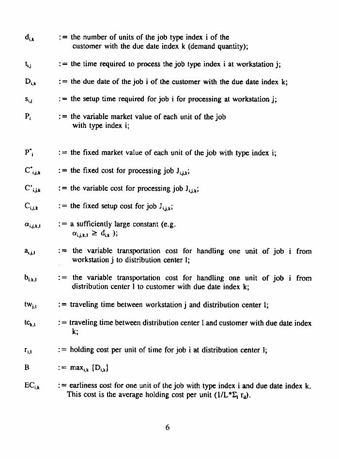
dur:= the number of units of the job type index i of thecustomer with the due date index k (demand quantity);

:= the time required to process the job type index i at workstation j;

D i ,k = the due date of the job i of the customer with the due date index k;

:= the setup time required for job i for processing at workstation j;

P1:= the variable market value of each unit of the jobwith type index i;

:= the fixed market value of each unit of the job with type index i;

C• i,j,k : = the fixed cost for processing job Jilk;

C' ii.k : = the variable cost for processing job Jilk;

Cu ir = the fixed setup cost for job Juk;

.= a sufficiently large constant (e.g.e i,j,k,1 di,k );

aija .= the variable transportation cost for handling one unit of job i fromworkstation j to distribution center 1;

:= the variable transportation cost for handling one unit of job i fromdistribution center 1 to customer with due date index k;

:= traveling time between workstation j and distribution center 1;

tCk.i : = traveling time between distribution center 1 and customer with due date indexk;

:= holding cost per unit of time for job i at distribution center 1;

B := max,,k {1),.k}

EC i,k : earliness cost for one unit of the job with type index i and due date index k.This cost is the average holding cost per unit (1/L*E1 rd).

6

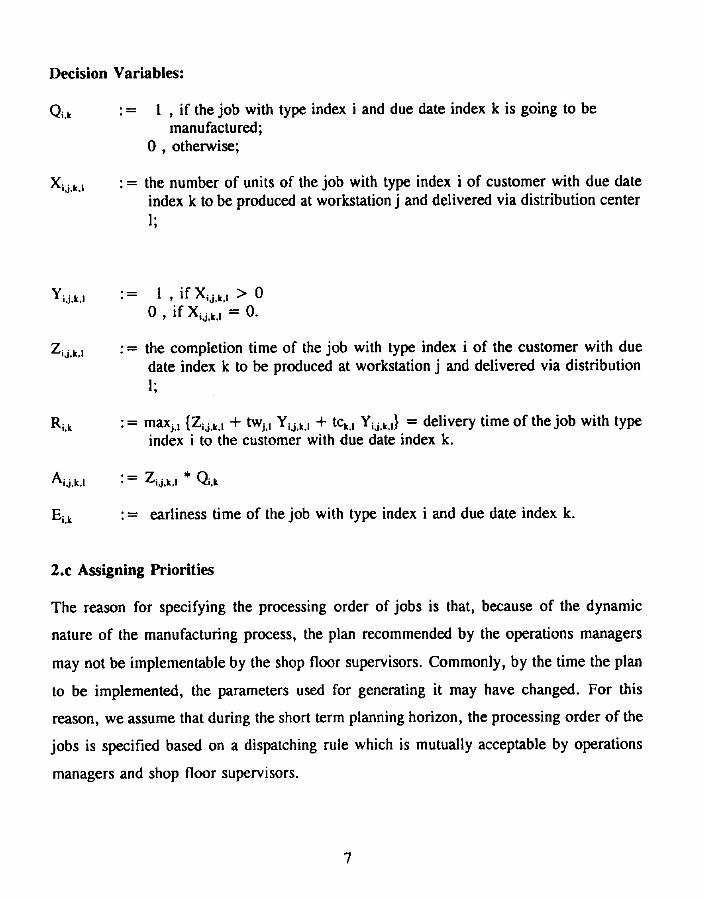
Decision Variables:

:= 1 , if the job with type index i and due date index k is going to bemanufactured;

0 , otherwise;

:= the number of units of the job with type index i of customer with due dateindex k to be produced at workstation j and delivered via distribution center1;

Yij,k,1 : = 1 , if Xi j,k,1 > 0

0 , if Xi j.k = O.

Zi : = the completion time of the job with type index i of the customer with duedate index k to be produced at workstation j and delivered via distribution1;

:= maxi, ' { Zi,j,k,1 tWj,I Y;J,k,1tCk.1 Y i à .k,i } delivery time of the job with typeindex i to the customer with due date index k.

= Zij,k,I * Qi,k

= earliness time of the job with type index i and due date index k.

2.c Assigning Priorities

The reason for specifying the processing order of jobs is that, because of the dynamic

nature of the manufacturing process, the plan recommended by the operations managers

may not be implementable by the shop floor supervisors. Commonly, by the time the plan

to be implemented, the parameters used for generating it may have changed. For this

reason, we assume that during the short term planning horizon, the processing order of the

jobs is specified based on a dispatching rule which is mutually acceptable by operations

managers and shop floor supervisors.

7

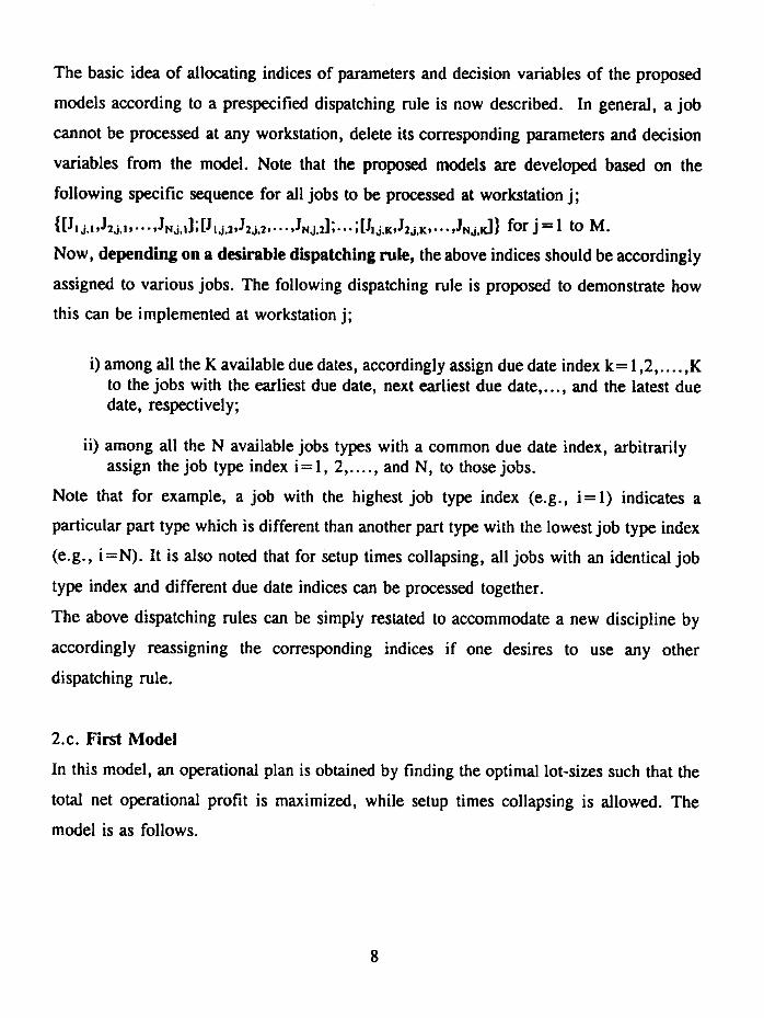
The basic idea of allocating indices of parameters and decision variables of the proposed

models according to a prespecified dispatching rule is now described. In general, a job

cannot be processed at any workstation, delete its corresponding parameters and decision

variables from the model. Note that the proposed models are developed based on the

following specific sequence for all jobs to be processed at workstation j;

{[J 1 J,1 e • • • yin ; 1.j,/,J212 • • • eJ lelj,2]; • • • ; [JI j,KeJ2j,Ke • • • eJNIK.11 for to M.

Now, depending on a desirable dispatching rule, the above indices should be accordingly

assigned to various jobs. The following dispatching rule is proposed to demonstrate how

this can be implemented at workstation j;

i) among all the K available due dates, accordingly assign due date index k=1,2,....,Kto the jobs with the earliest due date, next earliest due date,..., and the latest duedate, respectively;

ii) among all the N available jobs types with a common due date index, arbitrarilyassign the job type index i =1, 2,...., and N, to those jobs.

Note that for example, a job with the highest job type index (e.g., i=1) indicates a

particular part type which is different than another part type with the lowest job type index

(e.g., i=N). It is also noted that for setup times collapsing, all jobs with an identical job

type index and different due date indices can be processed together.

The above dispatching rules can be simply restated to accommodate a new discipline by

accordingly reassigning the corresponding indices if one desires to use any other

dispatching rule.

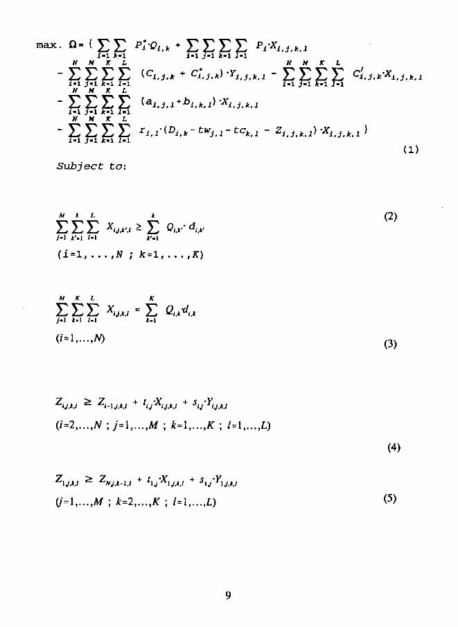
2.c. First Model

In this model, an operational plan is obtained by finding the optimal lot-sizes such that the

total net operational profit is maximized, while setup times collapsing is allowed. The

model is as follows.

8

P1 1CI, j,k,1N M K L

T.; k■1 1.1

( 1)

(C1,j,k + j,k)

I1,1 . (Di, X - twi, t ,

+ EEEEIon 1.1

max . = E E PI .Q12.1 1(4.

N MKL

EEEEj.1 k.1 i.1

N MKL

1.1 11F1 X.1 1.1N M K L

-EEEEE 1.1Subject ta:

M k L

EEEj.1 1.1

k (2)X ij,k',I E i,k'•

k'.I

(i=1,... ,N ; k=1,...,K)

M X L

E L Xrj.k,i = Ej.1 k.1 1.1

k.1

(i=1,...,N)

Z. > Z + t .X.. + s...Y..ij,k,1 i-lj,k,1 ij ij,k,1 tj,k,1

(i=2,...,N ; j=1,...,M ; k=1,...,K ; I= 1 , . . . ,L)

Z11,k,1 ZNj,k-1,1 + 1 j1j,k,1 + S 1 j1j,k,1

(j=1,...,M ; k=2,...,K ; 1=1,...,L)

(3)

(4)

(5)

9

R Zi,k + tw -YJ,I + tc k,I-Yij,k,1

(6)

(i=1,...,N ; j=1,...,M ; k=1,...,K ; 1 1,...,L)

15 D

(i=1,...,N ; k=1,...,K)

(7)

X < a -Y

(1=1,...,N ; j=1,...,M ; k=1,...,K ; 1 1,...,L)

(8)

; Zimvi ;

Qi,k 9 E 1 0 , 11 (9)

(i=1,...,N ; j=1,...,M ; k=1,...,K ; 1 1,...,L)

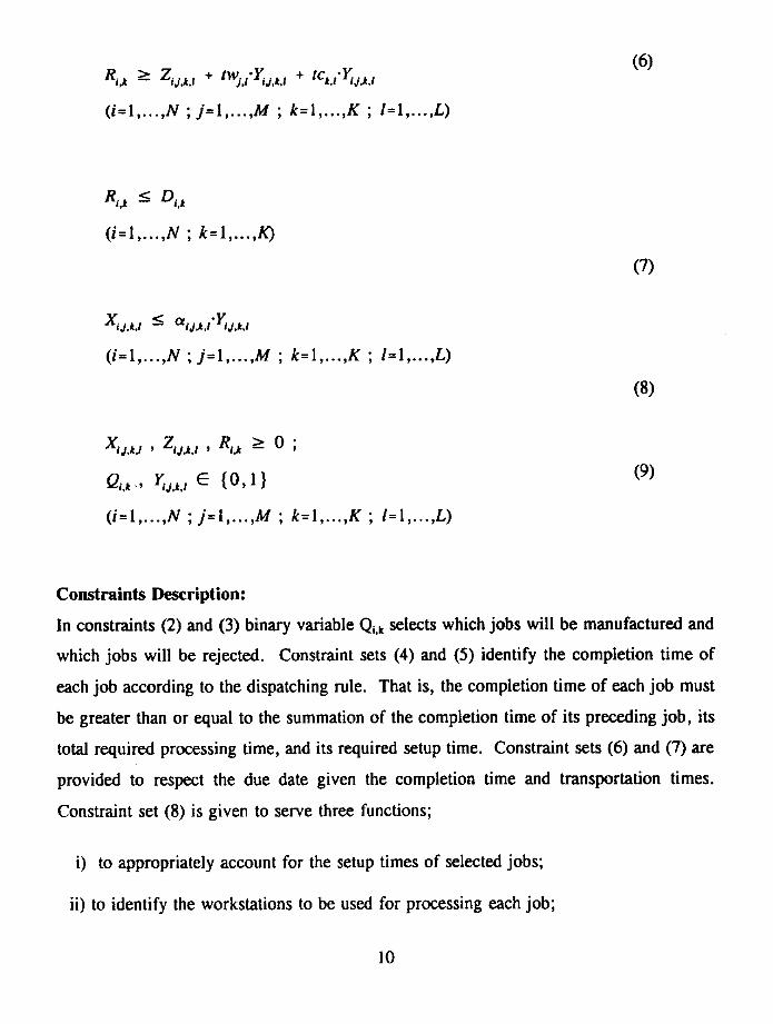
Constraints Description:

In constraints (2) and (3) binary variable (2,,k selects which jobs will be manufactured and

which jobs will be rejected. Constraint sets (4) and (5) identify the completion time of

each job according to the dispatching rule. That is, the completion time of each job must

be greater than or equal to the summation of the completion time of its preceding job, its

total required processing time, and its required setup time. Constraint sets (6) and (7) are

provided to respect the due date given the completion time and transportation times.

Constraint set (8) is given to serve three functions;

i) to appropriately account for the setup times of selected jobs;

ii) to identify the workstations to be used for processing each job;

10

iii) thirdly, to specify the inventory capacity of each workstation by appropriatelyselecting Cfii.k,i ; and to prevent allocation of excessive units to the transporter stationcorresponding to the workstation j.

Objective Function Description:

The first term of the objective function indicates the total fixed selling revenue, the second

represents the total variable selling revenue, the third takes cane of total fixed and variable

processing costs, the forth indicates the setup cost, the fifth represents the total

transportation cost while the last term indicates the holding costs.

It is obvious that the last term of the objective function is not linear due to multiplication

of Z, j,k,1 and X i jdo. However, this term can be linearized by the following assumption.

We assume that the production of a job for a given customer is first sent to the distribution

center(s) and upon the completion of the whole job, the products are transported from the

distribution center (s) to the customer. This assumption which is a good approximation

allows us to implement the EOQ concept and replace E . the average inventory

size in all distribution centers, Because a job with priority index i for a given

customer with due date index k may not be produced at all, we multiply d i,k/2 by Thus

we get Zuk 1 * di,k/2 * which is stil] not linear but can be easily linearized as the term

is composed of a continuous and a 0-1 variable. For this purpose we introduce the

continuous variable as defined in the list of variables. For the linearization we

need also to add the following constraints:

A i ^ B Qei,kj,k,I —

(i=1,...,N ; j=1,...,M ; k=1,...,K ; 1=1,...,L)

(10)

A Zij,k,1 ij,k,I

(i=1,...,N ; j=1,...,M ; k=1,...,K ; I=1,...,L)

(11)

11

(14)

N MKL

EEEEi-I j.1 k.I

NMKL r. di3,k,1 EEEE •k•A ,k.1j - I k . 1 L

-A i,Lk,1 B *( 1 - Qu)

(1=1,...,N ; j=1,...,M ; k=1,...,K ; 1=1,...,L)

(12)

The last term in the objective function, the inventory holding cost, will then change

from:

N M K L

E E E E r,` u - tWi f - !Cu -i•I j-I k-I 1.1

to:

(13)

Notice that the inventory cost is divided by L to get the average holding cost. Another way

of linearizing the last term is to replace (13) by:

N K

E E ECi.ki•I k.1

or the total earliness cost, and change constraint set (7) by:

Ri ,k Eik = Di,k • Qi,k

(1=1,...,N ; k=1,...,K)

(16)

The second approach aggregates more the inventory holding costs and reduces the

complexity of the model.

(15)

12

2.d. Second Model

In this model, an operational plan is obtained by finding the optimal lot-sizes such that the

total net operational profit is maximized, while setup times collapsing is not allowed. The

only difference between the second model and the first model is as follows; constraints (2)

and (3) in the first model are replaced by the following constraint (17). Thus, the

production quantity of each job type must equal its demand quantity.

Af L

E E XLbk,1 = QL0(1j.1 1-1 (17)

(i=1,...,N ; k=1,...,K)

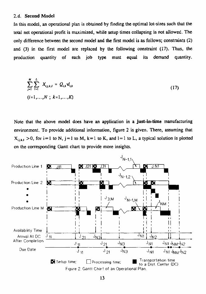
Note that the above model does have an application in a just-in-time manufacturing

environment. To provide additional information, figure 2 is given. There, assuming that

X ilka > 0, for i to N, j =1 to M, k=1 to K, and 1=1 to L, a typical solution is plotted

on the corresponding Gantt chart to provide more insights.

JN-1,1Production Line 1 SZ d11

Production Line 2•••

Production Une M

3,M N-1,MJ N M

I I

I : I1 41 1 JN2J N3 J1\11 JN1 JNMJN2

J 21 JI131 11 21• • •

11 21 J1\13 JINI1 JN1 JNMJN2

Availabilit y TimeArrivai At DC

Af ter Complet ion

Due Date

i> Setup lime;Figure

Transportation limeq Processing lime; to a Dist. Center (DC)

2. Gantt Chart of an Operational Plan.

13

3. SOLUTION ALGORITHMS

The models introduced in the previous section are fixed charge problems which are

represented by compatible mixed binary linear programming models and can be solved by

one of the standard algorithms which have been developed for solving such problems. For

a review of some of those algorithms see Shapiro (1979). In this paper, in order to

improve the computational performance of the model, it is assumed that each integral

variable can be treated as a continuous variable. Note that this latter assumption is justified

given that the production quantities at each workstation are sufficiently large.

There already exist computationally effective commercial softwares for solving our models.

For example, see IBM Mixed Integer Programming/370 Program Reference (1975) and

IBM Mathematical Programming system Extended/370 Program Reference Manual (1979),

or IBM Optimization Subroutine Library (OSL) (1990). These later softwares have

extensively been applied in Crowder, Johnson, and Padberg's (1983) study of large scale

binary linear programming problems. MPSARX developed by Van Roy and Wolsey

(1987) is a state-of-the-art Mathematical Programming system (MPS) that can be

implemented for solving our models. MPSARX consists of two modules, an MPS system

including all standard features and techniques for solving linear programming and mixed

integer programming and an Automatic Reformulaion Executor (ARX) whose goal it is to

speed up the solution of MIP problem, by producing an improved formulation based on

pre- and post-processing of the problem and dynamic cut generation procedures. For

additional references, see also Van Roy (1983), Van Roy and Wolsey (1983), Van Roy

(1989), Mikhalevich (1983), Jackson and O'Neil (1983), Cote and Laughton (1984), Glover

(1984), and Jeroslow (1984-a and b). Finally, for a review of the performance evaluation

literature of mixed binary programming algorithms, see von Randow (1985, pp. 198 and

199).

14

Obvisouly for large problem the models may be hard to solve to optimality with current

computer hard and software. In such cases one may therefore be forced to stop the

procedure early or to develop an appropriate heuristic. Solution techniques such as

Simulated Annealing or Tabu search have the potentials to be implemented for large scale

problems. Computational work is the subject of our current research to be reported in a

follow-up paper. We are confident that in the near future, more cpowerful computer

hardware will become available in an affordable price range. This will make our models

more accessible and applicable.

4. CONCLUDING REMARKS

Increasing implementation of Computer Integrated Manufacturing concepts raises issues in

planning of production and distribution of an IMS. The issues relate to interaction and

impacts of different production and distribution decisions on company profit. In order to

tackle these issues we extended the models developed by Pourbabai (1991). The extended

models have considered the integrated tradeoffs among several marketing, manufacturing,

and distribution factors on the net operational profit during the short term planning horizon.

The models can be distinguished from many other available models because of the fact that

they always result in an optimal feasible solution. The following propositions indicate this

fact.

Proposition 1;

The proposed models result in optimal feasible solutions.

Proof

Because of the term Qu for i = 1 to N and k 1 to K, the proposed models are

guaranteed to have feasible solutions (e.g., all orders may be rejected). Then, from

standard arguments for mixed integer programming algorithms, the optimality can be

guaranteed.

The following proposition indicates that setup times collapsing could increase the net

operational profit during the planning horizon.

15

Proposition 2:

fi � fi*

Proof:

Setup times collapsing may shorten the completion times of some jobs. Thus, the maximum

of the net operational profit accordingly increase, which results in fi � Q..

In summary, the models provide insights for the decision makers. Depending on the

capabilities required for a specific application, an operations manager should select the

required features of the models before using them. The extension shows that the models

can be improved further if necessary by considering additional technological and

operational limitations and capabilities.

16

REFERENCES

1. Cote, G. and M.A. Laughton, (1984), Large Scale Mixed Integer Programming:Bender-type Heuristics, E.J. of Operational Research, 16, 327-333.

2. Crowder H., E. L. Johnson, and M. Padberg (1983), Solving Large-Scale Zero-One Linear Programming Problems, Operations Research, 31, 5, 803-834.

3. Glover, F., (1984), An Improved MIP Formulation for Products of Discrete andContinuous Variables, J. of Information & Optimization Science, (Dehli), 3,196-208.

4. Ham, I., Hitomi, K., and Yoshida, T., 1985. Group Technology: Applicationsto Production Management, International Sertes in ManagementScience/Operations Research, Kluwer-Nijhoff Publishing.

5. Hartley, J., 1984, FMS at Work, IFS (publications) Ltd., UK and North-Holland Publishing Co.

6. IBM Mixed Integer Programming/370 (MIP/370) Program Reference Manual,(1975), Form number SH19-1099, IBM Corporation.

7. IBM Mathematical Programming System Extended/370 (MPSX/370) ProgramReference Manual, (1979), form number SH19-1095, IBM Corporation.

8. IBM's OSL Reference Manual, (1990), IBM Corporation, NY, USA.

9. Jackson, R.H.F. and R.P. O'Neil, (1983), Mixed Integer Programming Systems,A Joint Publication of the Computer Programming Society, Washington, D.C.,USA, ca, 100 p.

10. Jeroslow, R.G., (1984), Representability in Mixed Integer Programming, 1:Characterization Results, Working Paper, Atlanta: Georgia Institute ofTechnology, School of Industrial and Systems Engineering, 59 p.

11. Jeroslow, r.G., (1984), Representability in Mixed Integer Programming, 1: ALattice of Relaxations, Working Paper, Atlanta: Georgia Institute ofTechnology, School of Industrial and Systems Engineering, 79 p.

12. Mikhalevich, V.S., L. V. Volkovich, A.F., Voloshin, and S.O., Maschenko,(1983), A Successive Approach to Solution of Mixed Problems of LinearProgramming, (Russian), Kibernetika (Kiev), 1, 34-39.

17

13. Pourbabai, B., (1989-a), A Strategic Integrated Marketing and ProductionPlanning Model, Int. J. of Integrated Manufacturing Systems, 2, 6, 339-345.

14. Pourbabai, B., (1989-b), Components of a Decision Support System forComputer Integrated Manufacturing, in Int. J. of Integrated Manufacturing, 1,4,253-261.

15. Pourbabai, B., (1989-b), A Short Term Production Planning and SchedulingModel, to appear in Int. J. of Engineering Costs and Production Economics.

16. Pourbabai, B., (1991), Developing A Startegic Marketing and Production Planfor An Integrated Manufacturing System: With Setup Time Collasping, WorkingPaper, Dept. of Mechanical Engineering, The University of Maryland, U.S.A.

17. Randy, P.G., (1983), The Design and Operation of FMS, FlexibleManufacturing Systems, IFS (publications) Ltd., UK North-Holland PublishingCol.

18. Shapiro, J., (1979), Mathematical Programming: Structures and Algorithms,New York, Wiley.

19. Van Roy, T.J., (1983), Cross Decomposition for Mixed Integer Programming,Mathematical Programming, 25, 46-63.

20. Van Roy, T.J., and L.A. Wolsey, (1983), Valid Inequalities for Mixed 0-1Programs, CORE Discussion Paper 8316, Louvain-la-Neuve: Center forOperations Research and Economics, 19 p.

21. Van Roy, T.J., and L.A. Wolsey, (1987), Solving Mixed 0-1 IntegerProgramming by Automatic Reformulatio, Operations Research, 35, 45-57.

22. Van Roy, T.J. (1989), A Profit-maximizing Plant-loading Model with DemandFill-rate Constraints, Journal of Operational Research Society, 40, 1019-1027.

23. Von Randow, R. (1985), Integer Programming and Related Areas, ClassifiedBibliography, 1981-1984, Lecture Notes in Economics and MathematicalSystems, (ed. R. von Randow), Springer-Verlag.

24. Waghodekar, P.K. and Sahu, S., (1983), Group Technology: A ResearchBibliography, Research, 20, 4, 225-249.

18