Stock price synchronicity and liquidity

Available online at www.sciencedirect.com

Journal of Financial Markets 16 (2013) 414–438

1386-4181/$ -

http://dx.doi.

$We than

participants

Technology,

International

Workshop on

Si for excellen

the Research

support fromnCorrespon

E-mail ad

bizkwj@nus.

www.elsevier.com/locate/finmar

Stock price synchronicity and liquidity$

Kalok Chana,n, Allaudeen Hameedb, Wenjin Kangc

aDepartment of Finance, Hong Kong University of Science and Technology, Clear Water Bay, Hong KongbDepartment of Finance, NUS Business School, National University of Singapore, 15 Kent Ridge Drive, Singapore

119245, SingaporecHanqing Advanced Institute of Economics and Finance, Renmin University of China, Beijing, P.R. China

Received 27 July 2011; received in revised form 28 August 2012; accepted 29 September 2012

Available online 3 January 2013

Abstract

We argue and provide evidence that stock price synchronicity affects stock liquidity. Under the relative

synchronicity hypothesis, higher return co-movement (i.e., higher systematic volatility relative to total

volatility) improves liquidity. Under the absolute synchronicity hypothesis, stocks with higher systematic

volatility or beta are more liquid. Our results support both hypotheses. We find all three illiquidity

measures (effective proportional bid-ask spread, price impact measure, and Amihud’s illiquidity measure)

are negatively related to stock return co-movement and systematic volatility. Our analysis also shows that

larger industry-wide component in returns improves liquidity. We find that improvement in liquidity

following additions to the S&P 500 Index is related to the stock’s increase in return co-movement.

& 2013 Published by Elsevier B.V.

JEL classification: G19

Keywords: Liquidity; Price synchronicity; Systematic volatility

see front matter & 2013 Published by Elsevier B.V.

org/10.1016/j.finmar.2012.09.007

k Tarun Chordia, Gunter Strobl, Avanidhar Subrahmanyam, an anonymous referee, and seminar

at Lancaster University, Manchester University, Nomura (Tokyo), Queensland University of

Tsinghua University, University of Queensland, 2008 WFA Meetings (Hawaii), 2008 China

Conference in Finance (Dalian), 2008 NFA Asian FA Meetings, and the 4th Annual Central Bank

the Microstructure of Financial Markets (Hong Kong SAR) for useful comments. We thank Cheng

t research assistance. Chan acknowledges the financial support from the General Research Fund of

Grants of Hong Kong (No. HKUST640308). Hameed and Kang gratefully acknowledge financial

the NUS Academic Research Grants.

ding author. Tel.: þ852 2358 7681.

dresses: [email protected] (K. Chan), [email protected] (A. Hameed),

edu.sg (W. Kang).


dx.doi.org/10.1016/j.finmar.2012.09.007

http://crossmark.dyndns.org/dialog/?doi=10.1016/j.finmar.2012.09.007&domain=pdf





mailto:[email protected]



K. Chan et al. / Journal of Financial Markets 16 (2013) 414–438 415

1. Introduction

Liquidity reflects the ability to trade large quantities of a security quickly, with minimaltrading cost and little price impact. Extensive research has examined the cross-sectionaland time-series variation of liquidity in the equity markets. A key determinant of liquidityis the volatility of underlying stocks. An increase in volatility of underlying stock returnsimplies that the liquidity providers will face higher adverse selection risk due to anincreased possibility of trading with informed investors, as well as higher inventory riskarising from order imbalances. As a result, higher asset price volatility leads to lower assetliquidity (e.g., Stoll, 1978, 2000; Ho and Stoll, 1981).

While studies have shown that an increase in volatility lowers liquidity, there is littleresearch on the separate effects of systematic volatility and idiosyncratic volatility onliquidity. According to the adverse selection models or inventory risk models, the effect ofsystematic volatility on liquidity should be different from that of idiosyncratic volatility,given that systematic risk can be hedged to a certain extent. Furthermore, Baruch, Karolyi,and Lemmon (2007) and Baruch and Saar (2009), for example, argue that stock return co-movement affects the trading activity of a stock and therefore its liquidity. This is becausethe correlation of stock returns with the market measures the amount of market-wideinformation relative to firm-specific information. While market makers can observe themarket-wide information easily, it is more difficult for them to observe firm-specificinformation. When an individual stock is highly correlated with the market, marketmakers can rely more on the information observed from the market movement so that thestock price adjustments are less sensitive to its own order flow. Consequently, bothliquidity and informed traders choose to trade a larger proportion of the cross-listed assetin the exchange with the higher return correlation with the domestic assets. That is,proportionally more volume migrates to the market in which the cross-listed asset hasgreater correlation with the other assets traded on the market1 . Moreover,Subrahmanyam (1991) demonstrates that the introduction of a basket of securitiesprovides a preferred trading medium for uninformed liquidity traders, because adverseselection costs are typically lower in these markets than in markets for individual securities.This is related to the idea that the basket of securities is mainly affected by systematicreturns, as security-specific returns are diversified away, and consequently, is more liquid.

We test two empirical hypotheses. The first hypothesis is the relative synchronicityhypothesis, which predicts that stock return co-movement, or the R-square measure,positively affects the liquidity of a stock, as market makers learn more information fromthe market if the stock has more correlated fundamentals. The second hypothesis is theabsolute synchronicity hypothesis, which predicts that idiosyncratic volatility andsystematic volatility have different effects on liquidity, as market makers can hedge awaysystematic risk to a certain extent. Since a higher amount of market-wide informationlowers the adverse selection risk, we expect that an increase in systematic volatility will beaccompanied by an improvement in liquidity. We conduct empirical analysis based on asample of NYSE stocks from 1989 to 2008, and construct various liquidity measures,including proportional effective bid-ask spread, Kyle’s price impact measure, andAmihud’s illiquidity measure.

1Bhushan (1991) and Caballe and Krishnan (1994) also show the market maker is able to extract a greater

amount of information from the order flow of other securities when the stock co-moves more with the market.

K. Chan et al. / Journal of Financial Markets 16 (2013) 414–438416

Our empirical evidence supports both hypotheses. For the relative synchronicityhypothesis, we find that stock price synchronicity, a measure of stock return co-movement,has a negative relationship with all three illiquidity measures. For the absolutesynchronicity hypothesis, we also find that an increase in systematic volatility or marketbeta improves stock liquidity. Our results cannot be explained by cross-sectionaldifferences in firm size, price levels, institutional ownership, turnover, or idiosyncraticvolatility, which we use as control variables.We argue that our results are not caused by the reverse causality from liquidity to stock

return synchronicity, by showing that there is a similar relationship between a firm’searnings co-movement and liquidity. Our contention is that it is unlikely that stockliquidity drives earnings synchronicity. Based on market model regressions using return onassets (ROA), we find that firms with higher earnings co-movement have higher stockliquidity, confirming the causal effect of co-movement on liquidity.We also show that the co-variation in returns at the industry level is positively related

to liquidity: firms with greater industry-wide return co-movement exhibit higher liquidity.We also find a similar effect of higher industry-wide volatility and industry beta on stockliquidity. These results support our contention that a larger market or industry-widecomponent in returns reduces the adverse selection risk faced by liquidity providers andhence, improves the supply of liquidity. We demonstrate that the relationship betweenliquidity and stock price synchronicity is related to the extent of information asymmetry.When partitioning the sample into S&P 500 stocks versus non-S&P 500 stocks, we find thatthe relationship is stronger for non-S&P 500 stocks that have a higher degree ofinformation asymmetry. Our results also shed light on the indexing effect, where firms inthe major market index are likely to co-move more with the market and experience higherliquidity. In fact, we show that for firms being added to the S&P 500 Index, theimprovement in liquidity could be attributed to the increase in co-movement with themarket.The paper is organized as follows. Section 2 provides a discussion of the effect of stock

price synchronicity on liquidity. In Section 3 we describe the data and methodology.Section 4 contains the basic results on the relationship between liquidity and stock pricesynchronicity, while Section 5 contains extended analysis. Section 6 is the conclusion.

2. Effect of stock price synchronicity on liquidity

Stock price synchronicity, or the R-square measure, measures the proportion of sys-tematic volatility relative to the total volatility or idiosyncratic volatility. In this section, wesurvey related literature and discuss the potential effects of stock price synchronicity onliquidity. There is an extensive literature that predicts a negative relationship between assetprice volatility and asset liquidity (Stoll, 1978, 2000; Ho and Stoll, 1981). Previous studies,however, do not distinguish between systematic and idiosyncratic volatilities and examinehow each type of volatility may affect liquidity differently. Existing theories suggest thatidiosyncratic volatility has a larger impact on liquidity than systematic volatility. First, theadverse selection risk should primarily come from the idiosyncratic component. This isbecause while insiders or informed investors have advantages in collecting idiosyncratic(or firm-specific) information, it is more difficult for investors to possess a similaradvantage with regard to systematic (or market-wide) information. Second, inventory risk


is more likely to arise from idiosyncratic volatility as market makers can hedge againstmarket risk using stock index futures or derivative products.

While there is strong theoretical and empirical support for the negative associationbetween liquidity and idiosyncratic volatility2 , very little is known about the relationshipbetween liquidity and systematic volatility. In theory, the inventory risk associated with themarket can be hedged completely and there is no adverse selection risk due to the marketfactor. In this case, market makers do not need compensation for providing liquidity onaccount of systematic risk, so that there is no effect of systematic risk on liquidity. Inpractice, market makers are unable to completely eliminate market risk in their inventorycontrol, because hedging against market risk is either costly or imperfect. As for adverseselection risk, some of the private information that an insider obtains about a companymight be relevant for the market as a whole. Therefore, even for the systematic component,market makers need to protect themselves against adverse selection.

A number of studies document commonality in liquidity (Hasbrouck and Seppi, 2001;Huberman and Halka, 2001; Chordia, Roll, and Subrahmanyam, 2000). These papers findthat there are significant co-variations in liquidity among stocks. The existence ofcommonality in liquidity suggests that liquidity is driven by some common sources. Forexample, program trading of simultaneous large orders will exert common pressure ondealer inventories. Furthermore, institutional investors with similar investing styles mightexhibit correlated trading patterns, thereby inducing changes in inventory pressure acrossthe broad market. When dealing with a portfolio of stocks, market makers have to preparefor unexpected common pressure on inventories in their liquidity provision. Therefore, weexpect a negative impact of systematic risk of a stock on its liquidity, although it might notbe as strong as the idiosyncratic risk.

Furthermore, according to Subrahmanyam (1991), the amount of liquidity trading canbe endogenous, as there are discretionary liquidity traders who will choose to trade insecurities that have the least adverse selection risk. Since stocks of higher systematicinformation have less adverse selection, discretionary liquidity traders making portfolioadjustments can minimize liquidity costs by concentrating their trades in these stocks,resulting in a further improvement in liquidity.

So far, our discussion has been on the differential impact of systematic volatility andidiosyncratic volatility on liquidity. Baruch, Karolyi, and Lemmon (2007) and Baruch andSaar (2009) examine stock return co-movement, or the amount of market-wide volatilityrelative to firm-specific volatility, and demonstrate that it affects trading volume andthereby liquidity of a stock. These authors construct theoretical models in which themarket maker infers information based on order flows. The higher the return co-movementof a security, the more information the market maker is able to extract about the value ofthe security from the order flows of other securities in the market. This decreases theadverse selection risks, increases the incentives to trade the security, and lowers thesensitivity of the asset price to its own order flow. Hence, return co-movement is positivelyrelated to the liquidity of the asset. Baruch and Saar (2009) show that a stock is moreliquid when it is listed on a market where ‘‘similar’’ securities are traded, or when it has a

2Goyal and Santa-Clara (2003) provide empirical evidence on a positive relation between idiosyncratic volatility

and average stock returns. Bali, Cakici, Yan, and Zhang (2005), however, show that idiosyncratic volatility might

simply proxy for liquidity, so the empirical evidence documented in Goyal and Santa-Clara (2003) is a reflection

of liquidity premium. Spiegel and Wang (2005) also show idiosyncratic risk and liquidity are negatively correlated.


higher correlation with other securities. They find that stocks that switch their listing fromthe NASDAQ to the NYSE have return patterns more similar to securities already listedon the NYSE. They also document liquidity improvements for the switching firms that arepositively related to the degree of similarity in the return patterns. Baruch, Karolyi, andLemmon (2007) show the distribution of the trading volume across international stockexchanges is related to the correlation of the cross-listed asset returns that arise in therespective markets. Based on a sample of non-US stocks cross-listed on major US stockexchanges, they find that volume migrates to the exchange in which there is a greatercorrelation between the cross-listed asset returns and returns on other assets traded in themarket.We postulate two hypotheses based on the above discussions. The first is the relative

synchronicity hypothesis. Under this hypothesis, stocks with a higher degree of co-movement (i.e., a higher proportion of systematic volatility) are more liquid. The rationalefor the prediction is the learning effect as described in Baruch, Karolyi, and Lemmon(2007) and Baruch and Saar (2009), whereby learning about the information that drives theasset’s price improves liquidity. This hypothesis predicts a positive relationship betweenstock return co-movement and liquidity.The second is the absolute synchronicity hypothesis. Under this hypothesis, what affects

liquidity is the amount of systematic volatility and idiosyncratic volatility. This hypothesispredicts that after holding idiosyncratic volatility constant, higher systematic volatilityenhances liquidity. We conduct empirical tests of these two empirical hypotheses in thefollowing sections.

3. Data and methodology

The sample consists of all NYSE listed common stocks, identified by the Center forResearch in Security Prices (CRSP) share codes 10 and 11, over the period from January1989 to December 2008. We exclude stocks traded on the NASDAQ to avoid the influenceof differences in trading protocols. The CRSP dataset contains daily stock returns, dailytrading volume, number of shares outstanding, and yearly market capitalization. We filterout stocks with extreme price levels by discarding those with prices below $1 and above$999. For transaction-level data, we retrieve all trades and quotations from the New YorkStock Exchange Trade and Quote (TAQ) and the Institute for the Study of SecurityMarkets (ISSM)3 ,4.We construct several different proxies of firm level liquidity used in the prior literature.

The first measure of liquidity is the price-impact measure (l) introduced in Kyle (1985).For each firm, we use the price and quote information from TAQ to classify every trade asbuyer (seller) initiated, based on whether the transaction price is greater (lower) than theprevailing average of bid and ask quotes. Specifically, we follow the algorithm presented inLee and Ready (1991) in signing the transactions as buy and sell orders, matching tradingrecords to the most recent quote preceding the trade by at least 5 seconds. We aggregatethe buy and sell orders at the daily level and compute firm i’s net order imbalance at day t,OIBi,t, defined as the difference between the value of daily buyer and seller initiated trades.

3Anomalous transaction records are deleted according to the following filter rules: (i) negative bid-ask spread;

(ii) quoted spread 4$5; (iii) proportional quoted spread 420%; and (iv) effective spread/quoted spread 44.0.4We thank Tarun Chordia for sharing the TAQ-based measures of liquidity for the more recent years.


Our estimate of l for firm i is the coefficient from the following regression:

Ri,t ¼ ai þ liOIBi,t þ ei,t, ð1Þ

where Ri,t is the return on stock i on day t. Eq. (1) specifies that the stock price responds tothe net order imbalance. We have also estimated Eq. (1) by adding the return on themarket portfolio as an additional explanatory variable and obtain similar results.Therefore, the effect of net order imbalance on the stock returns, as measured by li, is notaffected when we control for the effect of market movement.

For each year, we estimate the daily price impact coefficient li by regressing dailyreturns on its corresponding order imbalance. Using a similar measure, Brennan andSubrahmanyam (1996) find that the price impact measure of liquidity is positively relatedto average stock returns, suggesting that illiquid stocks are compensated with liquiditypremium. Besides estimating li based on Eq. (1), we also do the estimation using atransaction-based measure and obtain similar results5 .

Our second liquidity measure is the effective bid-ask spread. Stoll (1978), Glosten andHarris (1988), and others show that bid-ask spread includes the adverse selection cost ofthe market maker trading with investors with superior information. We calculate theproportional effective spread based on two times the absolute difference between the tradeexecution price and the midquote, divided by the midquote. The daily averageproportional effective spreads for firm i are averaged each calendar year to generate ourannual spread measure, ESPRi.

The third liquidity measure is based on Amihud (2002) and does not rely on intradaytransaction data. It is calculated as the absolute daily return on stock i divided by the firm’sdaily dollar volume. Using this measure of the relative price change associated with tradingvolume, Amihud (2002) finds that firms with greater illiquidity earn higher expectedreturns, consistent with an illiquidity premium in returns. Acharya and Pedersen (2005)also use this illiquidity measure to investigate the effect of liquidity on security returns.Hasbrouck (2009) shows that the Amihud illiquidity measure is a robust measure of priceimpact, as posited in Kyle (1985).

It should be noted that the three measures are in fact illiquidity measures. If a stock isless liquid, it will have a higher bid-ask spread, its order flow will have a larger impact onstock prices, and the absolute price change per unit of volume will be greater. Therefore, anincrease in any of these measures is an indication of lower liquidity.

To investigate the relation between liquidity and the amount of market-wideinformation, we rely on the standard market model regressions to extract the market-wide component in returns. We start with the regression of weekly stock returns on stocki at week w (Ri,w) on the CRSP value-weighted weekly market returns (Rmkt,w):Ri,w ¼ aþ

Pþ1k ¼ �1 bi,kRmkt,w�k þ ei,w, where we include one week lead and lag of market

returns to account for any delayed adjustment in stock prices to market-wide information.Note that this is a standard market model, and does not include the net order imbalance asthe explanatory variable like Eq. (1), as our primary objective here is to distinguish return

5We estimate a transaction-based measure of Kyle’s l as an alternative. Here we follow the approach of

Brennan and Subrahmanyam (1996): let pj and qj denote the price and the signed quantity of the order fulfilled for

transaction j, and Dj denote the sign of the order. The regression Dpj¼aþlTqjþcDDjþej provides the estimates for

Kyle’s lT. It is a common practice to use Dpj¼ (pj�pj�1)/pj�1 as the regressor to ensure that our comparison of the

price impact estimate across different stocks is not affected by the price level. We repeat our analysis using the

transaction-based price impact measure for the period 1989–2003 and obtain qualitatively similar results.

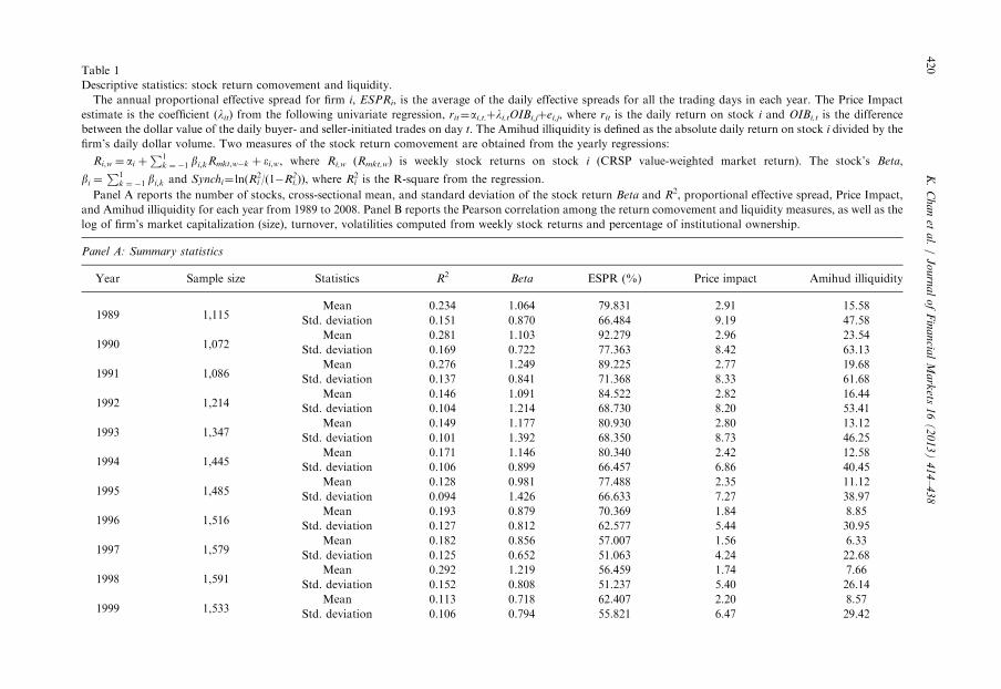
Table 1

Descriptive statistics: stock return comovement and liquidity.

The annual proportional effective spread for firm i, ESPRi, is the average of the daily effective spreads for all the trading days in each year. The Price Impact

estimate is the coefficient (lit) from the following univariate regression, rit¼ai,t,þli,tOIBi,jþei,j, where rit is the daily return on stock i and OIBi,t is the difference

between the dollar value of the daily buyer- and seller-initiated trades on day t. The Amihud illiquidity is defined as the absolute daily return on stock i divided by the

firm’s daily dollar volume. Two measures of the stock return comovement are obtained from the yearly regressions:

Ri,w ¼ ai þP1

k ¼ �1 bi,kRmkt,w�k þ ei,w, where Ri,w (Rmkt,w) is weekly stock returns on stock i (CRSP value-weighted market return). The stock’s Beta,

bi ¼P1

k ¼ �1 bi,k and Synchi¼ ln(R2i /(1�R2

i,)), where R2i is the R-square from the regression.

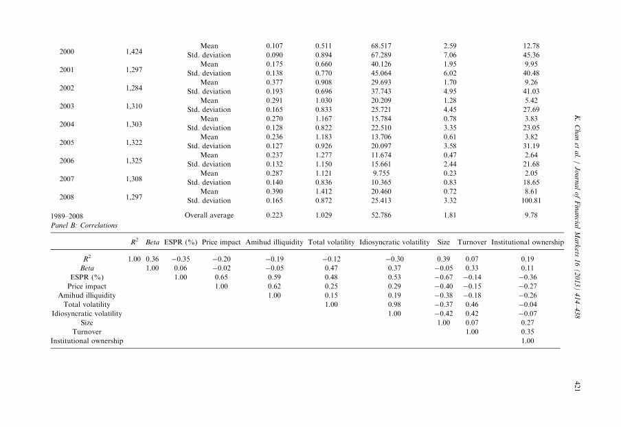
Panel A reports the number of stocks, cross-sectional mean, and standard deviation of the stock return Beta and R2, proportional effective spread, Price Impact,

and Amihud illiquidity for each year from 1989 to 2008. Panel B reports the Pearson correlation among the return comovement and liquidity measures, as well as the

log of firm’s market capitalization (size), turnover, volatilities computed from weekly stock returns and percentage of institutional ownership.

Panel A: Summary statistics

Year Sample size Statistics R2 Beta ESPR (%) Price impact Amihud illiquidity

1989 1,115Mean 0.234 1.064 79.831 2.91 15.58

Std. deviation 0.151 0.870 66.484 9.19 47.58

1990 1,072Mean 0.281 1.103 92.279 2.96 23.54

Std. deviation 0.169 0.722 77.363 8.42 63.13

1991 1,086Mean 0.276 1.249 89.225 2.77 19.68

Std. deviation 0.137 0.841 71.368 8.33 61.68

1992 1,214Mean 0.146 1.091 84.522 2.82 16.44

Std. deviation 0.104 1.214 68.730 8.20 53.41

1993 1,347Mean 0.149 1.177 80.930 2.80 13.12

Std. deviation 0.101 1.392 68.350 8.73 46.25

1994 1,445Mean 0.171 1.146 80.340 2.42 12.58

Std. deviation 0.106 0.899 66.457 6.86 40.45

1995 1,485Mean 0.128 0.981 77.488 2.35 11.12

Std. deviation 0.094 1.426 66.633 7.27 38.97

1996 1,516Mean 0.193 0.879 70.369 1.84 8.85

Std. deviation 0.127 0.812 62.577 5.44 30.95

1997 1,579Mean 0.182 0.856 57.007 1.56 6.33

Std. deviation 0.125 0.652 51.063 4.24 22.68

1998 1,591Mean 0.292 1.219 56.459 1.74 7.66

Std. deviation 0.152 0.808 51.237 5.40 26.14

1999 1,533Mean 0.113 0.718 62.407 2.20 8.57

Std. deviation 0.106 0.794 55.821 6.47 29.42

K.

Ch

an

eta

l./

Jo

urn

al

of

Fin

an

cial

Ma

rkets

16

(2

01

3)

41

4–

43

8420

2000 1,424Mean 0.107 0.511 68.517 2.59 12.78

Std. deviation 0.090 0.894 67.289 7.06 45.36

2001 1,297Mean 0.175 0.660 40.126 1.95 9.95

Std. deviation 0.138 0.770 45.064 6.02 40.48

2002 1,284Mean 0.377 0.908 29.693 1.70 9.26

Std. deviation 0.193 0.696 37.743 4.95 41.03

2003 1,310Mean 0.291 1.030 20.209 1.28 5.42

Std. deviation 0.165 0.833 25.721 4.45 27.69

2004 1,303Mean 0.270 1.167 15.784 0.78 3.83

Std. deviation 0.128 0.822 22.510 3.35 23.05

2005 1,322Mean 0.236 1.183 13.706 0.61 3.82

Std. deviation 0.127 0.926 20.097 3.58 31.19

2006 1,325Mean 0.237 1.277 11.674 0.47 2.64

Std. deviation 0.132 1.150 15.661 2.44 21.68

2007 1,308Mean 0.287 1.121 9.755 0.23 2.05

Std. deviation 0.140 0.836 10.365 0.83 18.65

2008 1,297Mean 0.390 1.412 20.460 0.72 8.61

Std. deviation 0.165 0.872 25.413 3.32 100.81

1989–2008 Overall average 0.223 1.029 52.786 1.81 9.78

Panel B: Correlations

R2 Beta ESPR (%) Price impact Amihud illiquidity Total volatility Idiosyncratic volatility Size Turnover Institutional ownership

R2 1.00 0.36 �0.35 �0.20 �0.19 �0.12 �0.30 0.39 0.07 0.19

Beta 1.00 0.06 �0.02 �0.05 0.47 0.37 �0.05 0.33 0.11

ESPR (%) 1.00 0.65 0.59 0.48 0.53 �0.67 �0.14 �0.36

Price impact 1.00 0.62 0.25 0.29 �0.40 �0.15 �0.27

Amihud illiquidity 1.00 0.15 0.19 �0.38 �0.18 �0.26

Total volatility 1.00 0.98 �0.37 0.46 �0.04

Idiosyncratic volatility 1.00 �0.42 0.42 �0.07

Size 1.00 0.07 0.27

Turnover 1.00 0.35

Institutional ownership 1.00

K.

Ch

an

eta

l./

Jo

urn

al

of

Fin

an

cial

Ma

rkets

16

(2

01

3)

41

4–

43

8421


fluctuations being explained by the market from those not explained. To test the relativesynchronicity hypothesis, we use the R-square of stock i (R2

i ) from the market model regression,which reflects the proportion of variation in return of stock i explained by market return. Sincethe R-square statistic is bounded between zero and one, the relative price synchronicity of stocki (Synchi) is obtained by taking the logit-transformation of R2

i : ln R2i = 1�R2

i

� �� . A higher

Synchi indicates a larger amount of market-wide information in stock i. We use two relatedmeasures of the absolute amount of market-wide information estimated from the regression.The first is the stock’s beta (bi ¼

Pþ1k ¼ �1 bi,k), which measures the sensitivity of return of stock i

to market return. The second measure is based on the systematic volatility estimated directlyfrom the market model regression. The systematic volatility, SysVoli, is the square root of the

systematic variance of stock i, i.e.,

ffiffiffiffiffiffiffiffiffiffiffiffiffiffiffiffiffiffiffiffiffiffiffiffiffib2i Var Rmktð Þ

q. The corresponding idiosyncratic volatility,

IdioVoli, is given by the square root of the difference between the total variance of stock i and thesystematic variance. We investigate whether the effect of systematic volatility on liquidity isdistinct from that due to idiosyncratic volatility.Table 1 contains summary statistics on our liquidity and price synchronicity measures for

each year from 1989 to 2008. Panel A reports the number of stocks, mean and standarddeviation of R-square, stock’s beta, as well as three liquidity measures (effective bid-askspread, price impact, and Amihud illiquidity measure). If we include all the stocks, the betasshould average to about one. But since our sample, which ranges between 1072 and 1591stocks per year, excludes NASDAQ stocks that tend to have higher betas, the average betaof our NYSE stocks is below one in a number of years, especially during the technologybubble period from 1999 to 2001.On the other hand, during the market turmoil of 2008,our sample stocks co-move with the market significantly, with an average beta of 1.412.The R-square from the market model regression averages to about 22.3% over the wholesample period, with yearly averages in the range of 10.7–39.0%. All three liquidity measuresdisplay a downward trend in illiquidity over time. For example, the effective bid-ask spreadis 0.798%, 0.923%, and 0.892% in the first three years, and declines steadily during thesample period to 0.137%, 0.116%, and 0.097% in 2005–2007, before it widens during thefinancial crisis of 2008. The other two liquidity measures also have a similar pattern. Overthe sample period, the price impact measure declined from 2.91 and hit the lowest point of0.23 in 2007, while the Amihud illiquidity measure declined from 15.58 and hit the lowestpoint of 2.05 in 2007. Panel A also presents the cross-sectional standard deviations. Theprice impact and Amihud illiquidity measures exhibit substantial cross-sectional dispersion,as their standard deviations are more than three times larger than the mean values.Panel B of Table 1 reports the unconditional correlations across firm-years among

R-square, beta, the liquidity proxies, and other firm-specific characteristics that we use ascontrol variables. In general, all the liquidity measures are highly correlated with each other,a result consistent with Korajczyk and Sadka (2008) and Hasbrouck (2009).We find that thedaily price impact coefficient l is highly correlated with both the effective spread and Amihudilliquidity. The R-squared measure is highly correlated with stock’s beta and idiosyncraticvolatility, with a correlation coefficient of 36% and �30%, respectively. The correlation oftotal volatility with idiosyncratic volatility is 98%, therefore the cross-sectional variation offirm volatility is primarily driven by the firm-specific component. Finally, the correlation ofliquidity measures with idiosyncratic volatility is higher than the correlations with the totalvolatility, providing preliminary evidence of the asymmetric effect of systematic volatility andidiosyncratic volatility on liquidity.


4. Empirical relationship between liquidity and stock price synchronicity

4.1. Explanatory variables

Several studies show that cross-security variation in liquidity can be explained by firmcharacteristics. Stoll (1978, 2000), Ho and Stoll (1981), and Harris (1994) show thatproportional bid-ask spreads are lower for bigger firms and high volume stocks as they areassociated with higher probability of finding a counterparty to trade and hence areassociated with lower inventory and order processing costs faced by the market maker.They also show that spreads are higher for stocks with high return variance due tocompensation for inventory risks, as well as the risk of trading with an informed trader.Hasbrouck (1991) reports that the price impact (and adverse selection risk) is higher forsmaller firms. Breen, Hodrick, and Korajczyk (2002) show that the price impact of trade isrelated to a number of firm-specific variables, including firm’s market capitalization,volume, absolute returns, and institutional ownership.

To test for the relative synchronicity hypothesis, we regress our liquidity measures on theproportion of systematic information in stock returns, measured by stock returnsynchronicity, Synch. To test for the absolute synchronicity hypothesis, we have a coupleof empirical specifications. One specification incorporates both idiosyncratic volatility,IdioVol, and systematic volatility, SysVol, as explanatory variables in the regression model,so that we can directly compare their distinct effects on liquidity. In another specification,we use beta to measure the absolute amount of systematic information, while controllingfor idiosyncratic volatility, IdioVol, in the regression model. The beta measure provides uswith an alternative functional form in measuring systematic risk.

We introduce a set of control variables that other studies have shown to affect firm levelliquidity, independent of the amount of market-wide information. The first is firm size,SIZE, which is equal to the log of market capitalization at the beginning of the year.Firm size is a proxy for adverse selection risk, which might affect the liquidity of the stock.The second variable is the institutional ownership, IO, or the percentage of the firm’s equityheld by institutional investors. For each year, the institutional holdings are measured as of theend of the previous year. Since a higher institutional ownership is accompanied by moreinformation disclosure and lower adverse selection risk, it should be accompanied by higherstock liquidity. The third is turnover, which is the ratio of daily trading volume to the numberof shares outstanding, averaged over the year. By construction, since turnover is endogenouslydetermined, it might capture the influences of other variables that explain our liquiditymeasures. Therefore, the effect of our synchronicity measures on the liquidity measures mightbe understated. The fourth variable is the inverse of price, 1/P, where P is the beginning of yearprice for the firm. When liquidity is measured by proportional effective spread, it is possiblethat the cross-sectional variation in liquidity is affected by differences in the price levels. Hence,we include the inverse of price as a control variable if the dependent variable is proportionaleffective spread.

4.2. Basic empirical results

Table 2 presents the results of the cross-sectional analysis, based on the fixed-effect panelregression, controlling for the time-trend in our liquidity measures. Panel A contains theresults using effective proportional bid-ask spread as the dependent variable. The t-statistics,

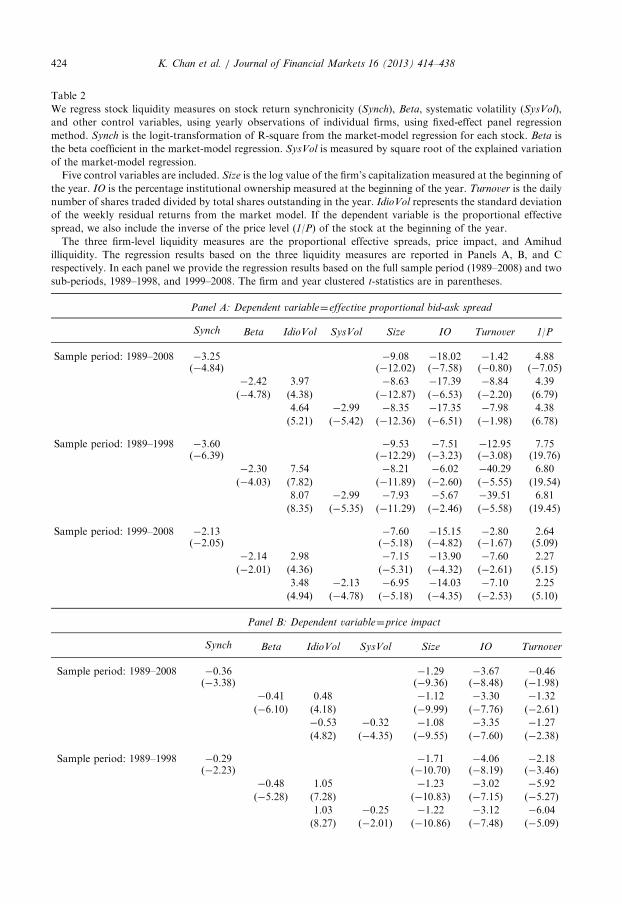
Table 2

We regress stock liquidity measures on stock return synchronicity (Synch), Beta, systematic volatility (SysVol),

and other control variables, using yearly observations of individual firms, using fixed-effect panel regression

method. Synch is the logit-transformation of R-square from the market-model regression for each stock. Beta is

the beta coefficient in the market-model regression. SysVol is measured by square root of the explained variation

of the market-model regression.

Five control variables are included. Size is the log value of the firm’s capitalization measured at the beginning of

the year. IO is the percentage institutional ownership measured at the beginning of the year. Turnover is the daily

number of shares traded divided by total shares outstanding in the year. IdioVol represents the standard deviation

of the weekly residual returns from the market model. If the dependent variable is the proportional effective

spread, we also include the inverse of the price level (1/P) of the stock at the beginning of the year.

The three firm-level liquidity measures are the proportional effective spreads, price impact, and Amihud

illiquidity. The regression results based on the three liquidity measures are reported in Panels A, B, and C

respectively. In each panel we provide the regression results based on the full sample period (1989–2008) and two

sub-periods, 1989–1998, and 1999–2008. The firm and year clustered t-statistics are in parentheses.

Panel A: Dependent variable¼effective proportional bid-ask spread

Synch Beta IdioVol SysVol Size IO Turnover 1/P

Sample period: 1989–2008 �3.25 �9.08 �18.02 �1.42 4.88(�4.84) (�12.02) (�7.58) (�0.80) (�7.05)

�2.42 3.97 �8.63 �17.39 �8.84 4.39

(�4.78) (4.38) (�12.87) (�6.53) (�2.20) (6.79)

4.64 �2.99 �8.35 �17.35 �7.98 4.38

(5.21) (�5.42) (�12.36) (�6.51) (�1.98) (6.78)

Sample period: 1989–1998 �3.60 �9.53 �7.51 �12.95 7.75(�6.39) (�12.29) (�3.23) (�3.08) (19.76)

�2.30 7.54 �8.21 �6.02 �40.29 6.80

(�4.03) (7.82) (�11.89) (�2.60) (�5.55) (19.54)

8.07 �2.99 �7.93 �5.67 �39.51 6.81

(8.35) (�5.35) (�11.29) (�2.46) (�5.58) (19.45)

Sample period: 1999–2008 �2.13 �7.60 �15.15 �2.80 2.64(�2.05) (�5.18) (�4.82) (�1.67) (5.09)

�2.14 2.98 �7.15 �13.90 �7.60 2.27

(�2.01) (4.36) (�5.31) (�4.32) (�2.61) (5.15)

3.48 �2.13 �6.95 �14.03 �7.10 2.25

(4.94) (�4.78) (�5.18) (�4.35) (�2.53) (5.10)

Panel B: Dependent variable¼price impact

Synch Beta IdioVol SysVol Size IO Turnover

Sample period: 1989–2008 �0.36 �1.29 �3.67 �0.46(�3.38) (�9.36) (�8.48) (�1.98)

�0.41 0.48 �1.12 �3.30 �1.32

(�6.10) (4.18) (�9.99) (�7.76) (�2.61)

�0.53 �0.32 �1.08 �3.35 �1.27

(4.82) (�4.35) (�9.55) (�7.60) (�2.38)

Sample period: 1989–1998 �0.29 �1.71 �4.06 �2.18(�2.23) (�10.70) (�8.19) (�3.46)

�0.48 1.05 �1.23 �3.02 �5.92

(�5.28) (7.28) (�10.83) (�7.15) (�5.27)

1.03 �0.25 �1.22 �3.12 �6.04

(8.27) (�2.01) (�10.86) (�7.48) (�5.09)


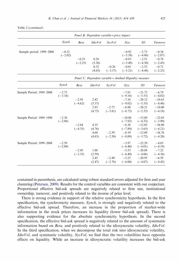
Table 2 (continued )

Panel B: Dependent variable¼price impact


Sample period: 1999–2008 �0.31 �0.92 �2.73 �0.38(�2.02) (�5.38) (�4.86) (�2.07)

�0.25 0.26 �0.83 �2.51 �0.78

(�2.25) (3.36) (�5.49) (�4.50) (�2.45)

0.32 �0.26 �0.81 �2.53 �0.71

(4.03) (�3.57) (�5.21) (�4.48) (�2.23)

Panel C: Dependent variable¼Amihud illiquidity measure


Sample Period: 1989–2008 �2.73 �7.81 �21.72 �6.79(�3.18) (�9.16) (�5.53) (�4.02)

�2.93 2.42 �7.18 �20.12 �10.63

(�4.62) (5.37) (�9.02) (�5.35) (�4.48)

2.93 �2.75 �6.90 �20.21 �10.00

(4.75) (�3.81) (�8.75) (�5.35) (�4.18)

Sample Period: 1989–1998 �2.38 �10.08 �15.89 �22.05(�2.06) (�7.92) (�4.32) (�3.90)

�2.84 4.35 �8.38 �12.05 �36.90

(�4.35) (4.76) (�7.89) (�3.65) (�4.21)

4.68 �2.59 �8.19 �12.09 �36.76

(4.83) (�2.50) (�8.09) (�3.72) (�4.20)

Sample Period: 1999–2008 �2.59 �5.97 �22.29 �4.65(�2.09) (�6.40) (�4.01) (�4.19)

�2.45 1.88 �5.53 �20.88 �7.22

(�2.35) (2.59) (�6.40) (�4.06) (�4.36)

2.45 �2.49 �5.25 �20.95 �6.59

(2.47) (�2.76) (�6.00) (�4.07) (�4.42)


contained in parenthesis, are calculated using robust standard errors adjusted for firm and yearclustering (Petersen, 2009). Results for the control variables are consistent with our conjecture.Proportional effective bid-ask spreads are negatively related to firm size, institutionalownership, turnover, and positively related to the inverse of price level.

There is strong evidence in support of the relative synchronicity hypothesis. In the firstspecification, the synchronicity measure, Synch, is strongly and negatively related to theeffective bid-ask spread. Therefore, an increase in the proportion of market-wideinformation in the stock prices increases its liquidity (lower bid-ask spread). There isalso supporting evidence for the absolute synchronicity hypothesis. In the secondspecification, the effective bid-ask spread is negatively related to the amount of systematicinformation based on Beta, and positively related to the idiosyncratic volatility, IdioVol.In the third specification, when we decompose the total risk into idiosyncratic volatility,IdioVol, and systematic volatility, SysVol, we find that the two volatilities have oppositeeffects on liquidity. While an increase in idiosyncratic volatility increases the bid-ask


spread, an increase of systematic volatility decreases it. Therefore, instead of adverselyaffecting liquidity, an increase in market-wide information actually attracts more liquiditytrading, resulting in a lower bid-ask spread. We have also partitioned the sample periodinto two sub-periods. We continue to find a negative relation between bid-ask spreads andsynchronicity (measured by R-squared or beta), as well as different impacts of systematicvolatility and idiosyncratic volatility on liquidity.Panel B of Table 2 contains the results using the price impact coefficient as the dependent

variable. Results are similar to those based on the effective bid-ask spread. Consistent with therelative synchronicity hypothesis, there is a significantly negative relationship between priceimpact and price synchronicity, indicating that the price impact of trades is smaller for stockswith higher co-movement with the market. Also consistent with the absolute synchronicityhypothesis, the price impact coefficient is negatively related to beta, once the idiosyncraticvolatility is controlled for. Finally, the effects of idiosyncratic volatility and systematic volatilityare asymmetric. While an increase in idiosyncratic volatility increases the price impact coefficient,an increase of systematic volatility decreases it. The results are again robust in both sub-periods6 .Similar findings are obtained when we use Amihud illiquidity as the dependent variable,

which are reported in Panel C of Table 2. Amihud illiquidity is lower for firms with higherstock return synchronicity. It is also lower for stocks of higher systematic volatility, andhigher betas, after controlling for the idiosyncratic volatility. We also obtain similar resultsin the sub-period analysis.In an unreported table available upon request, we apply the test statistics from Plosser,

Schwert, and White (1982) to compare the inference from the three regression specifications.The PSW test is applied to each stock in our sample and we fail to reject the null hypothesisthat the model is correctly specified for most of the stocks. When we measure liquidity usingbid-ask spreads, we do not reject the null hypothesis for 87–91% of firms across the threemodel specifications. Similarly, we fail to reject the PSW specification test for more than 84%of the firms when liquidity is computed based on the price impact, and 82% of the firms whenliquidity is computed based on Amihud illiquidity. This provides support for both the absolutesynchronicity hypothesis and the relative synchronicity hypothesis.

4.3. Robustness tests

4.3.1. Results based on changes in stock price synchronicity

One explanation for our findings is that stock price synchronicity reflects some firmcharacteristics being correlated with liquidity, other than firm size, institutional ownership,and turnover that we control for in the regression analysis. The relationship betweenilliquidity and stock price co-movement or systematic volatility could be a reflection ofomitted firm characteristics. As a robustness check, we employ an alternative set ofempirical specifications investigating the relationship using changes in liquidity andchanges in explanatory variables. Each year, we compute changes in stock returnsynchronicity, beta, systematic volatility, idiosyncratic volatility, as well as changes incontrol variables, and estimate the following specifications for the cross-sectional time-

6We obtain similar results when the price-impact measure in Eq. (1) is re-estimated after including market

returns as the explanatory variable.


series observations:

DLiquidityi,t ¼ aþ bUDSynchi,t þX

k

rkt UDCONTROLk

i,t þ ei,t: ð2Þ

DLiquidityi,t ¼ aþ bUDBetai,t þ cUDIdioVoli,t þX

k

rkt UDCONTROLk

i,t þ ei,t: ð3Þ

DLiquidityi,t ¼ aþ bUDSysVoli,t þ cUDIdioVoli,t þX

k

rkt DCONTROLk

i,t þ ei,t: ð4Þ

Results are reported in Table 3. Consistent with our previous regression results using thelevel variables, we find that changes in stock price synchronicity, DSynch, is negativelyrelated to changes in illiquidity measures, regardless of whether effective spreads, priceimpact, and Amihud illiquidity measures are used. In other words, after a firm experiencesan increase in stock price synchronicity, the stock will experience an improvement inliquidity. This evidence is in support of the relative synchronicity hypothesis. In the secondspecification, after controlling for the change of idiosyncratic volatility, DIdioVol, thechange in beta, DBeta, is negatively correlated with our illiquidity variables. Therefore,the result also supports the absolute synchronicity hypothesis. The third specification usesthe change in system volatility, DSysVol, and we obtain similar evidence only whenliquidity is measured by change in spreads. We obtain less statistically significant resultswhen we use change in Amihud illiquidity or a change in price impact measures. In thelatter specifications, the change of idiosyncratic volatility, DIdioVol, remains statisticallysignificant, but the change of systematic volatility is not. Overall, the negative relationshipbetween illiquidity and stock price synchronicity also holds when changes in theexplanatory variables are used, with stronger support for the relative synchronicityhypothesis.

4.3.2. Results based on frequently traded stocks

Another explanation for the evidence that illiquid stocks have lower co-movement withthe market is that betas are underestimated due to a thin trading problem. For thoseilliquid stocks that have higher bid-ask spreads, higher price impacts, and higher Amihudilliquidity measures, they will tend to have lower betas and lower systematic volatility. Wedo not think that such an explanation is likely, as our beta and R-square estimates alreadyadjust for delayed adjustments due to thin or non-synchronous trading using the leadingand lagging market returns.

Besides the thin trading, if large price impacts and transaction costs discourage trading,this can give rise to another mechanism through which the liquidity affects the stock returnsynchronicity. Here, large transaction costs deter arbitrageurs from trading in the stock,while other stocks are moving due to common information. Consequently, for theseilliquid stocks, their prices adjust only to large deviations from fundamental values, andhence, their synchronicity with the market will be lower. Panel A of Table 4 presentsadditional analysis based on stocks that do not have any zero trading volume days in theyear as a robustness test. In this way, we eliminate the illiquid stocks and examine stocksthat are less prone to the infrequent trading problem. We also examine the impact ofremoving stocks that have low number of trades each day, and require that stocks have atleast an average of 10 trades per day. The results are presented in Panel B of Table 4.

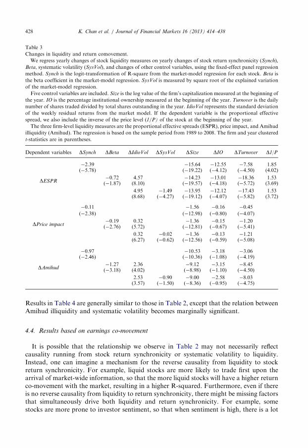
Table 3

Changes in liquidity and return comovement.

We regress yearly changes of stock liquidity measures on yearly changes of stock return synchronicity (Synch),

Beta, systematic volatility (SysVol), and changes of other control variables, using the fixed-effect panel regression

method. Synch is the logit-transformation of R-square from the market-model regression for each stock. Beta is

the beta coefficient in the market-model regression. SysVol is measured by square root of the explained variation

of the market-model regression.






The three firm-level liquidity measures are the proportional effective spreads (ESPR), price impact, and Amihud

illiquidity (Amihud). The regression is based on the sample period from 1989 to 2008. The firm and year clustered

t-statistics are in parentheses.

Dependent variables DSynch DBeta DIdioVol DSysVol DSize DIO DTurnover D1/P

DESPR

�2.39 �15.64 �12.55 �7.58 1.85(�5.78) (�19.22) (�4.12) (�4.50) (4.02)

�0.72 4.57 �14.23 �13.01 �18.36 1.53(�1.87) (8.10) (�19.57) (�4.18) (�5.72) (3.69)

4.95 �1.49 �13.95 �12.12 �17.43 1.53(8.68) (�4.27) (�19.12) (�4.07) (�5.82) (3.72)

DPrice impact

�0.11 �1.56 �0.16 �0.45

(�2.38) (�12.98) (�0.80) (�4.07)

�0.19 0.32 �1.36 �0.15 �1.20(�2.76) (5.72) (�12.81) (�0.67) (�5.41)

0.32 �0.02 �1.36 �0.13 �1.21(6.27) (�0.62) (�12.56) (�0.59) (�5.08)

DAmihud

�0.97 �10.53 �3.18 �3.06(�2.46) (�10.36) (�1.08) (�4.19)

�1.27 2.36 �9.12 �3.15 �8.45(�3.18) (4.02) (�8.98) (�1.10) (�4.50)

2.53 �0.90 �9.00 �2.58 �8.03(3.57) (�1.50) (�8.36) (�0.95) (�4.75)


Results in Table 4 are generally similar to those in Table 2, except that the relation betweenAmihud illiquidity and systematic volatility becomes marginally significant.

4.4. Results based on earnings co-movement

It is possible that the relationship we observe in Table 2 may not necessarily reflectcausality running from stock return synchronicity or systematic volatility to liquidity.Instead, one can imagine a mechanism for the reverse causality from liquidity to stockreturn synchronicity. For example, liquid stocks are more likely to trade first upon thearrival of market-wide information, so that the more liquid stocks will have a higher returnco-movement with the market, resulting in a higher R-squared. Furthermore, even if thereis no reverse causality from liquidity to return synchronicity, there might be missing factorsthat simultaneously drive both liquidity and return synchronicity. For example, somestocks are more prone to investor sentiment, so that when sentiment is high, there is a lot

Table 4

Liquidity and return co-movement for non-zero trading volume stocks.


and other control variables, based on the fixed-effect panel regression method. The sample consists of yearly

observations of stocks that do not have any zero trading volume days in the year. Synch is the logit-

transformation of R-square from the market-model regression for each stock. Beta is the beta coefficient in the

market-model regression. SysVol is measured by square root of the explained variation of the market-model

regression.






The three firm-level liquidity measures are the proportional effective spreads, price impact, and Amihud

illiquidity. The regression is based on the sample period from 1989 to 2008. The firm and year clustered t-statistics

are in parentheses.

Panel A: Non-zero trading volume stocks

Dependent variables Synch Beta IdioVol SysVol Size IO Turnover 1/P

ESPR

�2.96 �7.23 �15.36 0.25 4.37(�5.65) (�11.28) (�8.67) (0.21) (6.09)

�1.49 4.20 �6.51 �14.49 �7.72 3.82(�3.09) (4.61) (�11.31) (�7.15) (�2.51) (5.59)

4.80 �2.55 �6.26 �14.30 �6.90 3.80(5.42) (�5.18) (�11.01) (�7.29) (�2.27) (5.60)

Price impact

�0.24 �0.71 �2.08 �0.25(�5.03) (�11.86) (�10.28) (�2.66)

�0.16 0.36 �0.56 �1.80 �0.95(�3.99) (4.65) (�11.97) (�8.41) (�3.41)

0.40 �0.19 �0.55 �1.80 �0.90(5.51) (�4.71) (�11.83) (�8.53) (�3.12)

Amihud

�1.08 �3.05 �9.75 �3.97(�2.67) (�6.60) (�3.09) (�4.18)

�1.05 1.90 �2.24 �8.15 �7.53(�2.01) (3.56) (�8.59) (�2.94) (�3.98)

2.19 �1.31 �2.12 �8.10 �7.16(2.98) (�1.78) (�9.20) (�2.99) (�4.30)

Panel B: Non�zero trading volume stocks whose average daily number of traders is more than 10


ESPR

�2.95 �7.09 �15.13 0.38 4.32(�5.60) (�10.99) (�8.48) (0.35) (6.09)

�1.41 4.16 �6.35 �14.15 �7.63 3.78(�3.02) (4.62) (�10.89) (�6.89) (�2.53) (5.58)

4.81 �2.53 �6.10 �13.97 �6.80 3.76(5.43) (�5.23) (�10.59) (�7.03) (�2.28) (5.58)

Price Impact

�0.22 �0.67 �2.01 �0.22(�4.80) (�12.31) (�9.97) (�2.66)

�0.12 0.35 �0.53 �1.73 �0.90(�3.53) (4.71) (�11.65) (�8.21) (�3.53)

0.38 �0.18 �0.50 �1.72 �0.85


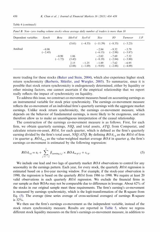
Table 4 (continued )

Panel B: Non�zero trading volume stocks whose average daily number of traders is more than 10


(5.61) (�4.53) (�11.59) (�8.35) (�3.23)

Amihud �0.98 �2.84 �9.32 �3.79(�2.45) (�6.13) (�2.98) (�3.87)

�0.90 1.86 �2.02 �7.69 �7.32(�1.72) (3.42) (�8.19) (�2.84) (�3.80)

2.15 �1.25 �1.89 �7.62 �6.95(2.88) (�1.69) (�9.05) (�2.88) (�4.09)


more trading for these stocks (Baker and Stein, 2004), which also experience higher stockreturn synchronicity (Barberis, Shleifer, and Wurgler, 2005). To summarize, since it ispossible that stock return synchronicity is endogenously determined, either by liquidity orother missing factors, one cannot ascertain if the empirical relationship that we reportreally reflects the impact of synchronicity on liquidity.To address this issue, we construct co-movement measures based on accounting earnings as

an instrumental variable for stock price synchronicity. The earnings co-movement measurereflects the co-movement of an individual firm’s quarterly earnings with the aggregate marketearnings. Unlike stock return synchronicity, the earnings co-movement measure, whichdepends on the behavior of fundamental earnings, is more likely to be exogenous, and cantherefore allow us to make an unambiguous interpretation of the causal relationship.The construction of the earnings co-movement measure is as follows. First, for each

firm, we obtain quarterly earnings, NIQ, and total assets, ATQ, from Compustat, andcalculate return-on-asset, ROA, for each quarter, which is defined as the firm’s quarterlyearning divided by the firm’s total asset, NIQ/ATQ. By defining ROAi.q as the ROA of firmi in quarter q, ROAm.q as the value-weighted market average ROA in quarter q, the firm’searnings co-movement is estimated by the following regression:

ROAi,q ¼ ai þX1

j ¼ �2

bearning,i,j � ROAm,qþj þ ei,q: ð5Þ

We include one lead and two lags of quarterly market ROA observations to control for anyseasonality in the earnings pattern. Each year, for every stock, the quarterly ROA regression isestimated based on a five-year moving window. For example, if the stock-year observation is1990, the regression is based on the quarterly ROA from 1986 to 1990. We require at least 20valid observations in each quarterly ROA regression. We exclude the financial firms inour sample as their ROAs may not be comparable due to differences in leverage. About 62% ofthe stocks in our original sample meet these requirements. The firm’s earning’s co-movementis measured by earnings synchronicity, which is the logit-transformation of the R-square fromEq. (5). The average (time series average of cross-sectional averages) of earnings R-squareis 32%.We then use the firm’s earnings co-movement as the independent variable, instead of the

stock return synchronicity measure. Results are reported in Table 5, where we regressdifferent stock liquidity measures on the firm’s earnings co-movement measure, in addition to

Table 5

Liquidity and earnings comovement.

We regress stock liquidity measures on earnings’ co-movement measures and other control variables. To

construct firm’s earnings’ co-movement measures, we regress quarterly return-on-asset (ROA) of an individual

firm on one lead and two lags of quarterly value-weighted market average ROA. The firm’s earning’s co-

movement is measured by earnings synchronicity, which is the logit-transformation of the R-square from the

regression equation. The three firm-level liquidity measures are the proportional effective spreads, price impact,

and Amihud illiquidity. A total of four control variables are included. Size is the log value of the firm’s

capitalization measured at the beginning of the year. IO is the percentage institutional ownership measured at the

beginning of the year. Turnover is the daily number of shares traded divided by total shares outstanding in the

year. IdioVol represents the standard deviation of the weekly residual returns from the market model. If

the dependent variable is the proportional effective spread, we also include the inverse of the price level (1/P) of

the stock at the beginning of the year. The regression results are based on the 1989–2008 sample period. The firm

and year clustered t-statistics are in parentheses.

Dependent variables Earnings synchronicity IdioVol Size I.O. Turnover 1/P

ESPR

�0.93 3.69 �8.21 �20.10 �8.46 4.27

(�2.11) (4.76) (�11.02) (�7.28) (�2.56) (6.40)

�3.21

(�3.23)

Price impact

�0.09 0.54 �1.05 �3.88 �1.39

(�1.84) (4.42) (�8.48) (�7.44) (�2.69)

�0.19

(�3.18)

Amihud

�0.37 1.88 �6.36 �21.69 �8.36

(�1.20) (3.80) (�8.60) (�6.20) (�3.06)

�0.97

(�2.62)


the control variables. In the first two specifications, we use bid-ask spread and price impact asthe dependent variables, and find the coefficients of earnings synchronicity to be negative andstatistically significant. This indicates that a stock experiences less illiquidity when theearnings comovement is higher. The evidence is slightly weaker in the last specification whenAmihud’s illiquidity measure is used—the coefficient of earnings synchronicity is significantlynegative in the univariate regression, but insignificant in the multivariate regression whenother control variables are included. But overall, results in Table 5 confirm that there iscausality going from (fundamental) return co-movement to the liquidity.

5. Extension of analysis

5.1. Co-movement due to industry effects

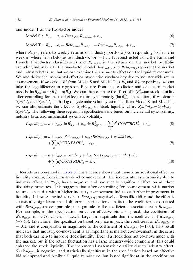
Since our focus is on the impact of systematic information on liquidity, we also examinethe influence of industry-wide information, separate from market returns. We ask whethergreater industry-wide information also attracts liquidity trading, which results in furtherimprovement in liquidity. We do this by computing the beta and synchronicity measuresbased on a two-factor model with market and industry factors, and compare them withthose based on a one-factor market model. We denote model S as the one-factor model


and model T as the two-factor model:

Model S : Ri,w ¼ ai þ Betamkt,iRmkt,j,w þ ei,w ð6Þ

Model T : Ri,w ¼ ai þ Betamkt,iRmkt,j,w þ BetaIND,iRind,j,w þ ei,w ð7Þ

where Rind,j,w refers to weekly returns on industry portfolio j corresponding to firm i inweek w (where firm i belongs to industry j, for j¼1,y,17, constructed using the Fama andFrench 17-industry classification) and Rmkt,j,w is the return on the market portfolioexcluding industry j. In the two-factor model, Betamkt,i and BetaIND,i represent the marketand industry betas, so that we can examine their separate effects on the liquidity measures.We also derive the incremental effect on stock price synchronicity due to industry-wide returnco-movement. If we denote R2 from Model S and Model T as R2

S and R2T, respectively, we can

take the log-difference in regression R-square from the two-factor and one-factor marketmodels: ln(R2

diff)¼ ln(R2T)�ln(R

2S). We can then estimate the effect of ln(R2

diff)on stock liquidityafter controlling for the market-level return synchronicity (ln(R2

S)). In addition, if we denoteSysVolS and SysVolT as the log of systematic volatility estimated from Model S and Model T,we can also estimate the effect of SysVoldiff on stock liquidity where SysVoldiff¼SysVolT�

SysVolS. The following three regression specifications are based on incremental synchronicity,industry beta, and incremental systematic volatility:

Liquidityi,t ¼ aþ bmktUlnR2S,i,t þ bidsUlnR2

diff ,i,t þX

k

dkt CONTROLk

i,t þ ei,t: ð8Þ

Liquidityi,t ¼ aþ bmktUBetamkt,i,t þ bidsUBetaIND,i,t þ cUIdioVoli,t

þX

k

dkt CONTROLk

i,t þ ei,t: ð9Þ

Liquidityi,t ¼ aþ bmktUSysVolS,i,t þ bidsUSysVoldiff ,i,t þ cUIdioVoli,t

þX

k

dkt CONTROLk

i,t þ ei,t: ð10Þ

Results are presented in Table 6. The evidence shows that there is an additional effect onliquidity coming from industry-level co-movement. The incremental synchronicity due toindustry effect, ln(R2

diff), has a negative and statistically significant effect on all threeilliquidity measures. This suggests that after controlling for co-movement with marketreturns, a security with a higher industry co-movement induces a further improvement inliquidity. Likewise, the industry beta BetaIND,i negatively affects illiquidity and the effect isstatistically significant in all different specifications. In fact, the coefficients associatedwith BetaIND,i are comparable in magnitude to the coefficients associated with Betamkt,i.For example, in the specification based on effective bid-ask spread, the coefficient ofBetaIND,i is �9.78, which, in fact, is larger in magnitude than the coefficient of Betamkt,i

(�8.53). Likewise, in the specification based on price impact, the coefficient of BetaIND,i is�1.02, and is comparable in magnitude to the coefficient of Betamkt,i (�1.03). This resultindicates that industry co-movement is as important as market co-movement, in the sensethat both can help to improve stock liquidity. Even if a stock does not co-move much withthe market, but if the return fluctuation has a large industry-wide component, this couldenhance the stock liquidity. The incremental systematic volatility due to industry effect,SysVoldiff,i, is negative, and statistically significant in the specification based on effectivebid-ask spread and Amihud illiquidity measure, but is not significant in the specification

Table 6

Liquidity and return comovement: effect of industry return comovement.

We estimate return comovement from a one-factor model and a two-factor model as follows:

Model S : Ri,w ¼ aþ Betamkt,iRmkt,j,w þ ei,w;

Model T : Ri,w ¼ aþ Betamkt,iRmkt,j,w þ BetaIND,iRind,j,w þ ei,w,

where Rindj,w refers to weekly returns on industry j portfolio corresponding to firm i, (j¼1,..,17 constructed using

the Fama and French 17-industry classification) and Rmktj,w is the return on the market portfolio excluding industry j.

The R2 from Model S and Model T are denoted as R2S and R2

T respectively. The incremental effect of industry-wide co-

movement is measured by the log-difference in regression R-square from the two-factor and single-factor market

models, denoted as ln(R2diff,i,t)¼ ln(R

2T)�ln(R

2S). SysVoldiff is similarly defined as the log difference between the systematic

volatility estimates from Model S and Model T correspondingly. The following regressions are reported:

Liquidityi,t ¼ aþ bmktUlnR2S,i,t þ bidsUlnR2

diff ,i,t þX

k

dkt CONTROLk

i,t þ ei,t

Liquidityi,t ¼ aþ bmktUBetamkt,i,t þ bidsUBetaIND,i,t þ cUIdioVoli,t þX

k

dkt CONTROLk

i,t þ ei,t:

Liquidityi,t ¼ aþ bmktUSysVolS,i,t þ bidsUSysVoldiff ,i,t þ cUIdioVoli,t þX

k

dkt CONTROLk

i,t þ ei,t:

IdioVol is the idiosyncratic volatility, CONTROL are control variables that include firm size (SIZE), institutional

ownership (IO), stock turnover (turnover), and the inverse of the price level (1/P). The three firm-level liquidity

measures are the proportional effective spreads (ESPR), price impact, and Amihud illiquidity (Amihud). The regression

is based on the sample period from 1989 to 2008. The firm and year clustered t-statistics are in parentheses.

Dependent

variablesln(R2

S) ln(R2diff) Betamkt BetaIND SysVolS SysVoldiff IdioVol Size IO Turnover 1/P

ESPR

�5.71 �5.25 �8.06 �18.13 �0.81 4.85(�8.28) (�6.56) (�11.95) (�7.86) (�0.48) (6.89)

�8.53 �9.78 4.12 �7.61 �17.99 �5.98 4.45(�8.68) (�9.18) (4.98) (�12.56) (�6.95) (�1.65) (6.78)

�5.75 �4.16 4.12 �7.74 �17.46 �6.91 4.45(�5.96) (�3.00) (4.69) (�12.16) (�6.45) (�1.80) (6.75)

Price impact

�0.57 �0.46 �1.19 �3.64 �0.41

(5.27) (�5.10) (�8.57) (�8.33) (�1.80)

�1.03 �1.02 0.46 �1.03 �3.39 �1.06

(�8.59) (�7.08) (4.53) (�9.69) (�7.83) (�2.25)

�0.46 �0.15 0.45 �1.06 �3.36 �1.18(�2.88) (�1.01) (4.46) (�8.96) (�7.38) (�2.28)

Amihud

�3.90 �2.82 �7.22 �21.46 �6.49(�4.00) (�3.89) (�8.67) (�5.48) (�3.95)

�8.02 �7.84 2.35 �6.68 �20.55 �8.82(�6.62) (�5.00) (�5.15) (�8.98) (�5.32) (�4.20)

�4.49 �2.08 2.31 �6.73 �20.16 �9.51(�3.28) (�2.23) (5.62) (�8.63) (�5.12) (�4.09)


based on price impact measure. Overall, the evidence in Table 6 provides support for theincremental effect of relative and absolute synchronicity with industry returns on liquidity.

5.2. Comparison between S&P 500 and non-S&P 500 stocks

We attribute the relationship between stock price synchronicity and liquidity to theadverse selection faced by liquidity providers. Such a relationship should not be uniform


across stocks, but be stronger (weaker) when the degree of information asymmetry ishigher (lower). We partition the stocks into two sub-samples, one based on S&P 500 stocksand the other based on non-S&P stocks, and investigate whether there is any differencebetween the two. Compared with S&P 500 stocks, non-S&P 500 stocks have less analystcoverage and smaller institutional ownership and are subject to a higher degree ofinformation asymmetry. We therefore expect that the relationship between stock pricesynchronicity and liquidity to be more pronounced for non-S&P 500 stocks than for S&P500 stocks.We obtain data on the list of firms that belong to the S&P 500 Index from Compustat.

We use the yearly variable S&P Primary Index Marker (CPSPIN) to identify stocks thatare included in the S&P 500 Index at the beginning of each year. We then pool all stockstogether in the regression analysis but include a dummy variable, NSPDummy, which isequal to one for the observations of non-S&P 500 stocks, and 0 otherwise. In theregression, we interact the dummy variable with other explanatory variables to investigateany differential effect between S&P 500 stocks and non-S&P 500 stocks.Results are presented in Table 7. In all specifications, we find that the negative

relationship between stock price synchronicity and illiquidity measures is morepronounced for non-S&P 500 stocks. Regardless of which illiquidity measure we use,the interaction terms involving Synch, Beta, and SysVol are all significantly negative.Therefore, the effect of return synchronicity on illiquidity is larger for non-S&P 500 stocks,which is consistent with our conjecture that these stocks have a higher degree ofinformation asymmetry. Furthermore, the main effect of beta and SysVol becomesinsignificant when the interaction terms are included. This implies that most of the maineffect of synchronicity on liquidity is driven by the non-S&P 500 stocks.

5.3. Liquidity impact of additions to S&P 500 index

There is extensive evidence of higher stock return commonality and liquidity for S&P500 Index component stocks. Furthermore, after a stock is added to the index, itexperiences an increase in trading volume and liquidity (Harris and Gural, 1986; Harfordand Kaul, 2005), as well as a higher beta or systematic co-movement (Vijh, 1994; Barberis,Shleifer, and Wurgler, 2005). Barberis, Shleifer, and Wurgler (2005) also provide evidencethat the increase in beta is not totally attributed to fundamental changes, but is also due tomarket friction and investor sentiment. In this section, we examine whether the changes inliquidity and beta subsequent to addition to the S&P 500 are related.Table 8 presents additional analysis based on stocks added to S&P 500 Index during the

period from 1989 to 2003. Only stocks that are added to S&P 500 Index will be eligible forinclusion in our analysis, with observations drawn from the year before and after theaddition to the index. We regress the liquidity proxy for each security in the combined pre-and post-addition years on different measures of market-wide information, controlvariables, and a S&P dummy variable that is equal to zero (one) during the pre (post) indexaddition years. In the first specification, each of the illiquidity measures is regressed on theS&P dummy variable, and we find that the coefficient for the dummy variable issignificantly negative, regardless of the illiquidity measures used. This confirms that thestock liquidity is higher after the stock is added to the index. In the second specification, weadd the synchronicity measure as an additional explanatory variable. While synchronicityis significantly negatively related to different illiquidity measures, the coefficient associated

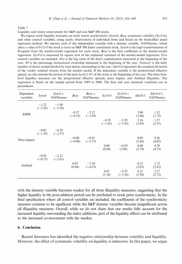
Table 7

Liquidity and return comovement for S&P and non S&P 500 stocks.


and other control variables, using yearly observations of individual firms and based on the fixed-effect panel

regression method. We interact each of the independent variable with a dummy variable, NSPDummy, which

takes a value of 0 (1) if the stock is (not) an S&P 500 Index constituent stock. Synch is the logit-transformation of

R-square from the market-model regression for each stock. Beta is the beta coefficient in the market-model

regression. SysVol is measured by square root of the explained variation of the market-model regression. Five

control variables are included. Size is the log value of the firm’s capitalization measured at the beginning of the

year. IO is the percentage institutional ownership measured at the beginning of the year. Turnover is the daily



spread, we also include the inverse of the price level (1/P) of the stock at the beginning of the year. The three firm-

level liquidity measures are the proportional effective spreads, price impact, and Amihud illiquidity. The

regression is based on the sample period from 1989 to 2008. The firm and year clustered t-statistics are in

parentheses.

Dependent

variablesSynch

Synch�

NSPDummyBeta

Beta�

NSPDummySysVol

SysVol�

NSPDummyIdioVol

IdioVol�

NSPDummy

ESPR

�1.22 �1.80(�2.38) (�3.58)

�0.27 �2.12 3.00 1.12(�0.53) (�3.45) (3.06) (1.72)

�0.59 �2.29 3.16 1.57(�1.45) (�5.45) (3.03) (2.55)

Price impact

�0.02 �0.29(�1.28) (�2.57)

�0.00 �0.41 0.08 0.36(�0.00) (�5.75) (2.86) (4.02)

0.00 �0.29 0.08 0.39(0.69) (3.88) (2.79) (4.53)

Amihud

�0.03 �2.12(�0.75) (�2.61)

0.05 �3.10 0.23 1.72(0.84) (�4.25) (2.05) (2.82)

0.05 �2.95 0.22 2.27(1.18) (�3.36) (1.98) (2.72)


with the dummy variable becomes weaker for all three illiquidity measures, suggesting that thehigher liquidity in the post-addition period can be attributed to stock price synchronicity. In thefinal specification where all control variables are included, the coefficients of the synchronicitymeasure continue to be significant while the S&P dummy variables become insignificant acrossall illiquidity measures. Overall, while we do not claim that our results fully account for theincreased liquidity surrounding the index additions, part of the liquidity effects can be attributedto the increased co-movement with the market.

6. Conclusion

Recent literature has identified the negative relationship between volatility and liquidity.However, the effect of systematic volatility on liquidity is unknown. In this paper, we argue

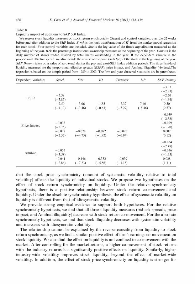
Table 8

Liquidity impact of additions to S&P 500 Index.

We regress stock liquidity measures on stock return synchronicity (Synch) and control variables, over the 52 weeks

before and after addition to the S&P Index. Synch is the logit-transformation of R2 from the market-model regression

for each stock. Four control variables are included. Size is the log value of the firm’s capitalization measured at the

beginning of the year. IO is the percentage institutional ownership measured at the beginning of the year. Turnover is the

daily number of shares traded divided by total shares outstanding in the year. If the dependent variable is the

proportional effective spread, we also include the inverse of the price level (1/P) of the stock at the beginning of the year.

S&P Dummy takes on a value of zero (one) during the pre- and post-S&P Index addition periods. The three firm-level

liquidity measures are the proportional effective spreads (ESPR), price impact, and Amihud illiquidity (Amihud).The

regression is based on the sample period from 1989 to 2003. The firm and year clustered t-statistics are in parentheses.

Dependent variables Synch Size IO Turnover 1/P S&P Dummy

ESPR

�3.93

(�2.93)

�5.58 �2.20

(�5.85) (�1.64)

�2.50 �3.06 �1.55 �7.32 7.46 0.50

(�4.10) (�3.46) (�0.63) (�5.27) (18.46) (0.57)

Price Impact

�0.039

(�2.33)

�0.033 �0.029

(�2.75) (�1.70)

�0.027 �0.078 �0.092 �0.025 0.002

(�2.32) (�4.75) (�1.92) (�0.94) (0.12)

Amihud

�0.054

(�2.48)

�0.057 �0.036

(�3.58) (�1.65)

�0.041 �0.146 �0.332 �0.039 0.028

(�2.86) (�7.23) (�5.56) (�1.18) (1.31)


that the stock price synchronicity (amount of systematic volatility relative to totalvolatility) affects the liquidity of individual stocks. We propose two hypotheses on theeffect of stock return synchronicity on liquidity. Under the relative synchronicityhypothesis, there is a positive relationship between stock return co-movement andliquidity. Under the absolute synchronicity hypothesis, the effect of systematic volatility onliquidity is different from that of idiosyncratic volatility.We provide strong empirical evidence to support both hypotheses. For the relative

synchronicity hypothesis, we find that all three illiquidity measures (bid-ask spreads, priceimpact, and Amihud illiquidity) decrease with stock return co-movement. For the absolutesynchronicity hypothesis, we find that stock illiquidity decreases with systematic volatilityand increases with idiosyncratic volatility.The relationship cannot be explained by the reverse causality from liquidity to stock

return synchronicity, as we find a similar positive effect of firm’s earnings co-movement onstock liquidity. We also find the effect on liquidity is not confined to co-movement with themarket. After controlling for the market returns, a higher co-movement of stock returnswith the industry returns has significantly positive effects on liquidity. Similarly, higherindustry-wide volatility improves stock liquidity, beyond the effect of market-widevolatility. In addition, the effect of stock price synchronicity on liquidity is stronger for


non-S&P 500 stocks than for S&P 500 stocks, suggesting that the extent of informationasymmetry is higher for non-S&P 500 stocks. Our paper also sheds light on the change inco-movement and liquidity after stocks are added to the S&P index. Previous literaturetends to treat them as separate issues. While one strand of research (e.g., Vijh, 1994;Barberis, Shleifer, and Wurgler, 2005) examines the increase in co-movement for stocksincluded in the index, another strand examines the effect on liquidity (Harris and Gural,1986; Harford and Kaul, 2005). Our paper shows that the two effects might be indeedrelated, as the increase of R-square is related to the rise in liquidity for those stocks addedto the S&P 500 Index. Overall, our evidence suggests that the degree of stock returnsynchronicity has a significant impact on asset liquidity.

References

Acharya, V., Pedersen, L., 2005. Asset pricing with liquidity risk. Journal of Financial Economics 77, 375–410.

Amihud, Y., 2002. Illiquidity and stock returns: cross-section and time-series effects. Journal of Financial Markets

5, 31–56.

Baker, M., Stein, J., 2004. Market liquidity as a sentiment indicator. Journal of Financial Markets 7, 271–299.

Bali, T., Cakici, N., Yan, X., Zhang, Z., 2005. Does idiosyncratic risk really matter? Journal of Finance 60,

905–929.

Barberis, N., Shleifer, A., Wurgler, J., 2005. Comovement. Journal of Financial Economics 75, 283–317.

Baruch, S., Karolyi, A., Lemmon, L., 2007. Multimarket trading and liquidity: theory and evidence. Journal of

Finance 62, 2169–2200.

Baruch, S., Saar, G., 2009. Asset returns and listing choice of firms. Review of Financial Studies 22, 2239–2274.

Bhushan, R., 1991. Trading costs, liquidity and asset holdings. Review of Financial Studies 4, 343–360.

Breen, W., Hodrick, L., Korajczyk, R., 2002. Predicting equity liquidity. Management Science 48, 470–483.

Brennan, M., Subrahmanyam, A., 1996. Market microstructure and asset pricing: on the compensation for

illiquidity in stock returns. Journal of Financial Economics 41, 441–464.

Caballe, J., Krishnan, M., 1994. Imperfect competition in a multi-security market with risk neutrality.

Econometrica 63, 695–704.

Chordia, T., Roll, R., Subrahmanyam, A., 2000. Commonality in liquidity. Journal of Financial Economics 56,

3–28.

Glosten, L., Harris, L., 1988. Estimating the components of the bid/ask spread. Journal of Financial Economics

21, 123–142.

Goyal, A., Santa-Clara, P., 2003. Idiosyncratic risk matters!. Journal of Finance 58, 975–1008.

Harford, J., Kaul, A., 2005. Correlated order flow: pervasiveness, sources and pricing effects. Journal of Financial

and Quantitative Analysis 40, 29–55.

Harris, L., 1994. Minimum price variations, discrete bid-ask spreads, and quotation sizes. Review of Financial

Studies 7, 149–178.

Harris, L., Gurel, E., 1986. Price and volume effects associated with changes in the S&P 500 list: new evidence for

the existence of price pressure. Journal of Finance 41, 851–860.

Hasbrouck, J., 1991. The summary informativeness of stock trades: an econometric analysis. Review of Financial

Studies 4, 571–595.

Hasbrouck, J., Seppi, D., 2001. Common factors in prices, order flows, and liquidity. Journal of Financial

Economics 59, 383–411.

Hasbrouck, J., 2009. Trading costs and returns for U.S. equities: estimating effective costs from daily data.

Journal of Finance 64, 1445–1477.

Ho, T., Stoll, H., 1981. Optimal dealer pricing under transactions and return uncertainty. Journal of Financial

Economics 9, 47–73.

Huberman, G., Halka, D., 2001. Systematic liquidity. Journal of Financial Research 24, 161–178.

Korajczyk, R., Sadka, R., 2008. Pricing the commonality across alternative measures of liquidity. Journal of

Financial Economics 87, 45–72.


Kyle, A.S., 1985. Continuous auctions and insider trading. Econometrica 53, 1315–1335.

Lee, C., Ready, M., 1991. Inferring trade direction from intraday data. Journal of Finance 46, 733–754.

Petersen, M., 2009. Estimating standard errors in finance panel data sets: comparing approaches. Review of

Financial Studies 22, 435–480.

Plosser, C., Schwert, G., White, H., 1982. Differencing as a test of specification. International Economic Review

23, 535–552.

Spiegel, M., Wang, X., 2005. Cross-Sectional Variation in Stock Returns: Liquidity and Idiosyncratic Risk.

Working Paper, Yale School of Management.

Stoll, H., 1978. The supply of dealer services in securities markets. Journal of Finance 33, 1133–1151.

Stoll, H., 2000. Friction. Journal of Finance 55, 1479–1514.

Subrahmanyam, A., 1991. A theory of trading in stock index futures. Review of Financial Studies 4, 17–51.

Vijh, A., 1994. S&P 500 trading strategies and stock betas. Review of Financial Studies 7, 215–251.

Documents

Stock price synchronicity and liquidity