Solar Energy 150 (2017) 485–499

Contents lists available at ScienceDirect

Solar Energy

journal homepage: www.elsevier .com/locate /solener

Statistical fault detection in photovoltaic systems

http://dx.doi.org/10.1016/j.solener.2017.04.0430038-092X/� 2017 Elsevier Ltd. All rights reserved.

⇑ Corresponding author.E-mail address: fouzi.harrou@kaust.edu.sa (F. Harrou).

Elyes Garoudja a, Fouzi Harrou b,⇑, Ying Sun b, Kamel Kara a, Aissa Chouder c, Santiago Silvestre d

a SET Laboratory, Electronics Department, Blida 1 University, BP 270 Blida, AlgeriabKing Abdullah University of Science and Technology (KAUST), Computer, Electrical and Mathematical Sciences and Engineering (CEMSE) Division, Thuwal 23955-6900, Saudi ArabiacElectrical Engineering Laboratory (LGE), University Mohamed Boudiaf of M’sila, BP 166, 28000, Algeriad Electronic Engineering Department, Universitat Politècnica de Catalunya, C/ Jordi Girona 1-3, Campus Nord UPC, 08034 Barcelona, Spain

a r t i c l e i n f o

Article history:Received 3 February 2017Received in revised form 25 March 2017Accepted 17 April 2017Available online 8 May 2017

Keywords:Fault detectionTemporary shadingPhotovoltaic systemsOne-diode modelStatistical monitoring charts

a b s t r a c t

Faults in photovoltaic (PV) systems, which can result in energy loss, system shutdown or even serioussafety breaches, are often difficult to avoid. Fault detection in such systems is imperative to improve theirreliability, productivity, safety and efficiency. Here, an innovative model-based fault-detection approachfor early detection of shading of PV modules and faults on the direct current (DC) side of PV systems isproposed. This approach combines the flexibility, and simplicity of a one-diode model with the extendedcapacity of an exponentially weighted moving average (EWMA) control chart to detect incipient changesin a PV system. The one-diode model, which is easily calibrated due to its limited calibration parameters,is used to predict the healthy PV array’s maximum power coordinates of current, voltage and power usingmeasured temperatures and irradiances. Residuals, which capture the difference between the measure-ments and the predictions of the one-diode model, are generated and used as fault indicators. Then, theEWMA monitoring chart is applied on the uncorrelated residuals obtained from the one-diode model todetect and identify the type of fault. Actual data from the grid-connected PV system installed at theRenewable Energy Development Center, Algeria, are used to assess the performance of the proposedapproach. Results show that the proposed approach successfully monitors the DC side of PV systemsand detects temporary shading.

� 2017 Elsevier Ltd. All rights reserved.

1. Introduction

1.1. The state of the art

Traditional sources of energy, such as oil, coal and nuclearenergy, have negative effects on human health, biodiversity,ecosystems and climate change. Nonetheless, industrial growthhas extensively increased global consumption of fossil fuels, andthe concomitant impacts on human health and the environment(Johansson, 1993). Renewable energy sources such as solar, windand biomass, are promising alternatives to conventional fossil fuelsbecause they are clean, sustainable, safe, and environment-friendlywith zero CO2 emissions (Panwar et al., 2011). One of the most sus-tainable and economically competitive renewable energy sourcesis solar photovoltaic (PV) energy (Zhao et al., 2015). Moreover,solar PV energy increases a country’s energy security by reducingdependence on fossil fuels.

Under practical conditions, faults are unavoidable in PV sys-tems, particularly on the direct current (DC) side where open cir-

cuit faults, short circuits faults, hotspot faults, and total andpartial shading faults are possible (Chouder and Silvestre, 2010;Hachana et al., 2016; Silvestre et al., 2015; Yahyaoui and Segatto,2017). Faults on the DC side of PV systems can result in energy loss,system shutdown and even in serious safety breaches (Brooks,2011; Alam et al., 2015). For example, two PV facilities in the US(a 383 KWp PV array in Bakersfield, CA and a 1.208 MWp powerplant in Mount Holly, NC) burned in 2009 and 2011, respectively(Brooks, 2011). The source for these accidents was a fault on theDC side that was not identified early (Vergura et al., 2009;Hariharan et al., 2016). If such faults in PV systems are not detectedpromptly, they can affect the system’s efficiency and profitability,as well as the health and safety of workers and community mem-bers. The detection of faults in PV systems is therefore crucial formaintaining normal operations by providing early fault warnings.Indeed, accurate and early detection of faults in a PV system is crit-ical to avoid the progression of faults and to reduce considerablyproductivity losses.

Several fault detection techniques for PV systems have beendeveloped. They are two main types of these techniques: processhistory-based approaches and model-based approaches. Process-history-based methods use implicit empirical models derived from

Fig. 1. The PV array installed on the roof of the CDER building in Algiers, Algeria(Arab et al., 2005).

486 E. Garoudja et al. / Solar Energy 150 (2017) 485–499

analysis of available data and rely on computational intelligenceand machine learning methods (Mekki et al., 2016; Shrikhandeet al., 2016; Hare et al., 2016; Suganthi et al., 2015; Silvestreet al., 2014; Tadj et al., 2014; Zhao et al., 2013). Mekki et al.(2016) proposed an artificial neural network to evaluate PV systemperformance under partial shading conditions. Chine et al. (2016)used an artificial neural network to detect short circuits in PVarrays. Tadj et al. (2014) proposed a fault-detection approachbased on fuzzy logic to detect possible solar panel abnormalities.Pavan et al. (2013) used a Bayesian neural network and polynomialregression to predict the effect of soiling in large-scale PV system.However, process-history-based methods require the availabilityof a relevant dataset that describes both healthy and faulty operat-ing conditions in a PV system.

On the other hand, model-based approaches compare analyti-cally computed outputs with measured values and signal an alarmwhen large differences are detected (Harrou et al., 2014). Severalmodel-based approaches to fault detection in PV systems havebeen reported in the literature using the one-diode model(Chouder and Silvestre, 2010; Vergura et al., 2009; Chouder andSilvestre, 2009; Chao et al., 2008). In one-diode-based fault detec-tion approaches, model parameters are determined by parameter-extraction methods from weather conditions and the datasheetfrom the PV module manufacturer (Garoudja et al., 2015; Abouet al., 2015; Chouder and Silvestre, 2010). Both irradiance and solarpanel temperature measurements are needed for such approachesto predict the maximum power point (MPP) of the PV system. Kanget al. (2012) used a Kalman filter to predict the power output of aPV system. Johnson et al. (2011) used a Fourier series to detect arcfaults in a PV system. Other approaches employed sophisticatedtools, such as time-domain reflectometry (TDR) (Munoz et al.,2011) and thermoreflectance imaging (TR) (Hu et al., 2014). TheTR method was proposed to detect the appearance of hot spotsinside PV systems (Hu et al., 2014). The TDR approach can detect,localize, and diagnose faults in PV systems, but the system mustbe turned off, which affects system productivity. TDR also requiressophisticated tools to introduce the input signal. Of course, theeffectiveness of model-based fault-detection approaches relies onthe accuracy of the models used.

1.2. Motivation and contributions

Until recently, statistical process control charts have not beenwidely used to monitor the performance of PV systems. Zhaoet al. (2013) proposed a statistical technique using three outlierrules to classify deviations. Recently, Platon et al. (2015) proposedto use the three-sigma rule for online fault detection in PV systems.However, the three-sigma rule, also known as the Shewhart chart(Montgomery, 2007), loses the ability to detect incipient faults inprocess data because it makes decisions based only on informationabout the process in the last observation. Incorporating informa-tion about the entire process history, including previous or recentobservations, into the decision rule can help to improve sensitivityto small shifts. The exponentially weighted moving average(EWMA) scheme incorporates information from the entire processhistory, rather than using only the most recent observation. Thismakes it more sensitive than the Shewhart chart to small anoma-lies. The main contribution of this work is to exploit the advantagesof the exponentially weighted moving average (EWMA) chart andthose of one-diode modeling for enhancing detection perfor-mances of PV systems, especially for detecting small faults in DCside of PV system and shading fault. Such a choice is mainly moti-vated by the greater ability of the EWMA metric to detect smallfault in process mean, which makes it very attractive as fault detec-tion approach. Note that the main advantage of EWMA chart is thatit can be easily implemented in real time because of the low com-

putational cost, which is not the case in a classifiers based methods(the classifier algorithms are performed offline rather than online).A decision can be made for each new sample by comparing thevalue of the EWMA decision statistic with the value of the thresh-old. An anomaly is declared if the EWMA statistic exceeds thethreshold. To do so, residuals, which are the differences betweenthe measured and predicted MPP for the current, voltage andpower, from the PV array simulation model are generated. Undernormal operating conditions, the residuals in a PV system are closeto zero due to measurement noise and errors, while they signifi-cantly deviate from zero when the system is faulty. Residuals areused as fault indicators. Then, an EWMA chart is used to monitorthe residuals to reveal abnormalities. Once the fault has beendetected, the next step is expected to determine its cause. The pro-posed approach can also effectively diagnose fault types based onthe output DC current and voltage. Indeed, fault diagnosis can helpthe operators and engineers in the process-monitoring scheme andtherefore significantly reduce the risk of safety problems or loss inprofitability. The proposed fault detection strategy has been vali-dated using measurements from the 9.54 kWp PV plant at theRenewable Energy Development Center in Algiers, Algeria.

The remainder of this paper is organized as follows. Section 2gives a brief overview of the grid-connected PV plant that provideddata for this study. In Section 3, one-diode model is reviewed. Sec-tion 4 introduces the EWMA chart and its use in fault detection.Section 5 applies the proposed fault-detection and diagnosis proce-dure to the PV plant in Algeria. Finally, Section 6 concludes with adiscussion and suggestions for future research directions.

2. The grid-connected PV system in Algiers, Algeria

We assessed our fault detection method using practical datacollected from a grid-connected photovoltaic (GCPV) systemlocated at Renewable Energy Development Center (CDER) inAlgiers, Algeria. This PV system operates from June 21st, 2004,and the output power by this system is injected directly into thenational electric distribution network without any storage device.This 90 module PV system 106 Wp is installed on the roof of theCDER building as shown in Fig. 1. This 9.54 kWp rated systemhas an output DC voltage of 125–450 V and an output AC voltageof 220 V. It comprises three sub-arrays of 30 modules each. Theoutputs of these three sub-arrays are connected to a single-phase2.5 KW PV inverter (IG30 Fronius). Each sub-array consists of 30Isofoton (106W-12 V) PV modules, which are grouped into twoparallel strings of fifteen PV modules in series. Irradiance measure-ments are collected with a Kipp & Zonen CM11 thermoelectricpyranometer and the temperature is measured with a K-type ther-mocouple. An Agilent 34970A data logger acquires the datathrough a connection to the local grid through an inverter, a safetycontrol box and a meter. When the utility grid is not energized the

Table 1Electrical characteristics of the Isofoton 106-12 PV module under standard testcondition.

Electrical characteristics of the solar panels tested in this study Value

Peak power (PMPP) 106 WVoltage at maximum power point (VMPP) 17.4 VCurrent at maximum power point (IMPP) 6.10 AOpen circuit voltage (Voc) 21.6 VShort circuit current (Isc) 6.54 A

E. Garoudja et al. / Solar Energy 150 (2017) 485–499 487

inverter immediately stops providing power to the grid. The maincomponents of the GCPV system are shown in Fig. 2.

The data from only one sub-array are used to simulate bothhealthy and faulty operating conditions under various meteorolog-ical conditions. The electrical characteristics of the Isofoton 106–12PV module are summarized in Table 1.

The standard test conditions for these solar panels were deter-mined at 25 �C and solar irradiance of 1000 W/m2. The real mea-surements (ie., MPP voltage and current) were collected everysecond.

2.1. Typical faults in PV systems

Generally, a PV system can be affected by different types offaults that can result in significant loss of power in a PV system.According to the fault duration, two types of faults can be distin-guished: temporary and permanent faults. Temporary faults, suchas shading, disappear after a certain period of time or after beingmanually cleared in cases of dust, leaves or bird dropping. ThePV system then returns to its normal operating conditions. Onthe other hand, permanent faults, including short circuits and opencircuits are persistent or ongoing. Three well-known faults com-monly occurred in the DC side of PV systems (short circuits, opencircuits and partial shading) are studied in this paper (see Fig. 3).

A short-circuit fault can affect cells, bypass diodes or modules.It is mainly due to the infiltration of water into modules or to badwiring between the module and the inverter. Additionally, aging ofPV modules, which is caused by long-term operation of the PV sys-tem, is one of the main sources of short-circuit faults. For example,there is a short-circuit fault at point ‘F1’ on the second string on theright of the PV array in Fig. 3.

An open-circuit fault may occur if any current path that is inseries to the load is accidentally removed or opened from a closedcircuit. Such a situation mainly occurs due to a break in wiresbetween PV modules or solar cells. An example of an open-circuit fault is shown at point at ‘F2’ in Fig. 3. Open-circuit faults

Fig. 2. The main components of grid-con

occur when a conductor is accidentally removed from the closedcircuit.

A partial shading fault occurs when part of the PV array isshaded while the other part is normally exposed to the solar irra-diance. This occurs due to several reasons including passage ofclouds, dirt on PV modules, snow, or any other light barrier. Nearbyobstacles might also interfere and cast shadows, resulting inreduced power output. Even a small amount of shade can dramat-ically reduce the output amperage of a PV system.

3. PV module modeling

Numerous models have been reported in the literature thatmodel energy production of PV cells. The one-diode model(ODM) is the most common model used to predict energy produc-tion from PV cells (Duffie and Beckman, 2013). This model is basedon modeling the solar cell as a light-generated current source con-nected in parallel with a diode with series and parallel resistancesaccounting for resistive losses (see Fig. 4).

ODM determines the resulting current and voltage given theparameters of the solar cell (McEvoy et al., 2012) as follows:

I ¼ Iph � I0 expqðV þ RsIÞ

nkBT

� �� 1

� �|fflfflfflfflfflfflfflfflfflfflfflfflfflfflfflfflfflfflfflfflfflfflffl{zfflfflfflfflfflfflfflfflfflfflfflfflfflfflfflfflfflfflfflfflfflfflffl}

Id

�V þ RsIRsh|fflfflfflffl{zfflfflfflffl}Ish

; ð1Þ

nected PV system used in this study.

Fig. 3. The faulty operating cases considered in this paper.

Fig. 4. Equivalent circuit of a solar cell based on a current source and a diode, withlosses represented by series and parallel resistance.

488 E. Garoudja et al. / Solar Energy 150 (2017) 485–499

where I and V are the generated current and voltage of the solar cell,respectively. Iph, also called the photogenerated current, corre-sponds to the amount of current generated by incoming photons;it is proportional to the irradiance and the area of the solar cell. I0is the dark saturation current, n is the diode’s ideality factor. Rs

and Rsh are the series and shunt resistances, respectively. kB is Boltz-mann’s constant (kB � 1:38064852� 10�23 J K�1). T is the cell’s tem-perature and q is the electronic charge (q � 1:60217662� 10�19 C).

The simulation of a PV array is comprised of three stages sum-marized next.

Step 1 : Model parameters extractionODM in Eq. (1) depends on the values of five unknownparameters (Iph; I0;n, Rs and Rsh), which determine theoverall performance of a solar cell. These parameters arenot provided in the manufacturer’s datasheet. Hence,accurate extraction of these parameters is a crucial stepin PV system modeling. Indeed, solar cell parametersextraction could be defined as an optimization problem,wherein the cost function to be minimized is defined asthe root mean square error (RMSE) between the measuredand the predicted I-V curves by ODM.

RMSE ¼ffiffiffiffiffiffiffiffiffiffiffiffiffiffiffiffiffiffiffiffiffiffiffiffiffiffiffiffiffiffiffiffiffiffiffiffiffiffiffiffiffiffiffiffiffiffiffiffiffiffiffiffiffiffiffiffiIm

Xm

i¼1f iðImeas;Vmeas; hÞ½ �2

r; ð2Þ

where

f ðImeas;Vmeas; hÞ ¼ Imeas

� Iph � I0 expqðVmeas þ RsImeasÞ

nkBT

� �� 1

� ���Vmeas þ RsImeas

Rsh

; ð3Þ

Imeas and Vmeas are the measured output current and voltage ofthe reference PV module respectively (they define the staticI-V curve measurements of the reference PV module), h isthe vector of the five unknowns electrical parameters[Iph; I0;n, Rs and Rsh],m stands for the number of experimentaldata used in the parameters extraction process. The static I-Vcurve of a reference PV module are measured using an I-Vcurve tracer when the module is isolated from the inverter.In practice, I-V curve tracer takes less than one second tomeasure the current–voltage (I-V) characteristic of the testedPV module. Of course, the aim of this optimization is to findthe optimal parameters values that minimize the objectivefunction and provides the lowest RMSE value. In this paper,these five parameters have been extracted using the ArtificialBee Colony (ABC) algorithm (Garoudja et al., 2015; Abouet al., 2015) on the basis of the real measured static (I-V) data,the predicted data obtained from the one diode model andthe available parameters in Table 1.

Step 2 : Model simulationThe identified parameters via ABC algorithm, which aregiven in Table 2, are used to predict the MPP coordinatesof current, voltage and power of the entire PV array. ThePV array model is simulated using PSIMTM/MatlabTM co-simulation. Using this co-simulation, the entire PV arrayis physically constructed (physical PV modules) as twoparallel PV string, of fifteen PV modules each. This modelrelies on access to both irradiance and solar panel temper-ature measurements to predict the MPP coordinates.

Step 3 : Model validationModel validation is possibly the most important step in PVarray modeling. In this step, the ability of the simulated

Table 2Extracted PV module parameters.

PV parameters Iph [A] I0 [A] n Rs [X] Rsh [X]

Value 6.54 1.11e�05 1.66 0.1474 202.6

E. Garoudja et al. / Solar Energy 150 (2017) 485–499 489

model to mimic accurately the real behavior of the moni-tored PV plan is evaluated. Specifically, the identified ODMparameters are used to build the entire PV array co-simulation model, then this later is used to mimic the realPV array behavior under different meteorological condi-tions. The input variables of the simulated model consistof real measured meteorological conditions of tempera-tures and irradiances. The output variables are the PVarray MPP coordinates of current, voltage and power. Thepredicted MPP coordinates of voltage and power obtainedfrom the simulated model are then compared to the realmeasured MPP coordinates collected from the real PVarray. Here, the co-simulation model is fitted to thefault-free data from the GCPV system described above.Fig. 5(a) and (b) respectively shows the measured and pre-dicted DC current and DC power for a cloudy day, June 24,

0 500 1000 1500Time [Min]

0

2

4

6

8

10

12

DC

cur

rent

[A]

(a)

Measured DC currentPredicted DC current

Fig. 5. Measured and predicted plot of DC curre

Measured current [A]

Pre

dict

ed c

urre

nt [A

]

2

3

4

5

6

7

8

9

10

11 r 2 = 0.96476 MAPE = 6.5693 RMSE = 0.19328

(a)

2 3 4 5 6 7 8 9 10 11

Fig. 6. Scatter plot of the measured and predicted DC

2008. This figure shows that the model suitably fits themeasured data, thus indicating that the selected parame-ters are satisfactory. This figure also shows that after sun-set and during periods of negligible irradiances, the systemcompletely shuts down. This is done to reduce power con-sumption and thereby increase overall efficiency. Scatterplot of the measured and predicted DC current and DCpower are presented in Fig. 6(a) and (b). These plots indi-cate that the PV array simulation model predicts the mea-sured DC current and DC power well.

In addition, to evaluate the quality of the simulation model withthe selected parameters, three numerical criteria are used: R2, themean absolute percent error (MAPE) and RMSE. These were calcu-lated as follows:

R2 ¼ 1�Pm

t¼1ðyt � ytÞ2Pmt¼1ðyt �meanðYÞÞ2

; ð4Þ

RMSE ¼ffiffiffiffiffiffiffiffiffiffiffiffiffiffiffiffiffiffiffiffiffiffiffiffiffiffiffiffiffiffiffiPm

t¼1ðyt � ytÞ2m

s; ð5Þ

Time [Min]0 500 1000 1500

DC

pow

er [W

]

0

500

1000

1500

2000

2500

(b)

Measured DC powerPredicted DC power

nt (a) and DC power (b) for June 24, 2008.

0 500 1000 1500 2000 2500

Measured power [W]

600

800

1000

1200

1400

1600

1800

2000

2200

2400

2600

Pre

dict

ed p

ower

[W]

(b)

r2 = 0.9591 MAPE = 6.0708 RMSE=0.03

current (a) and DC power (b) for June 24, 2008.

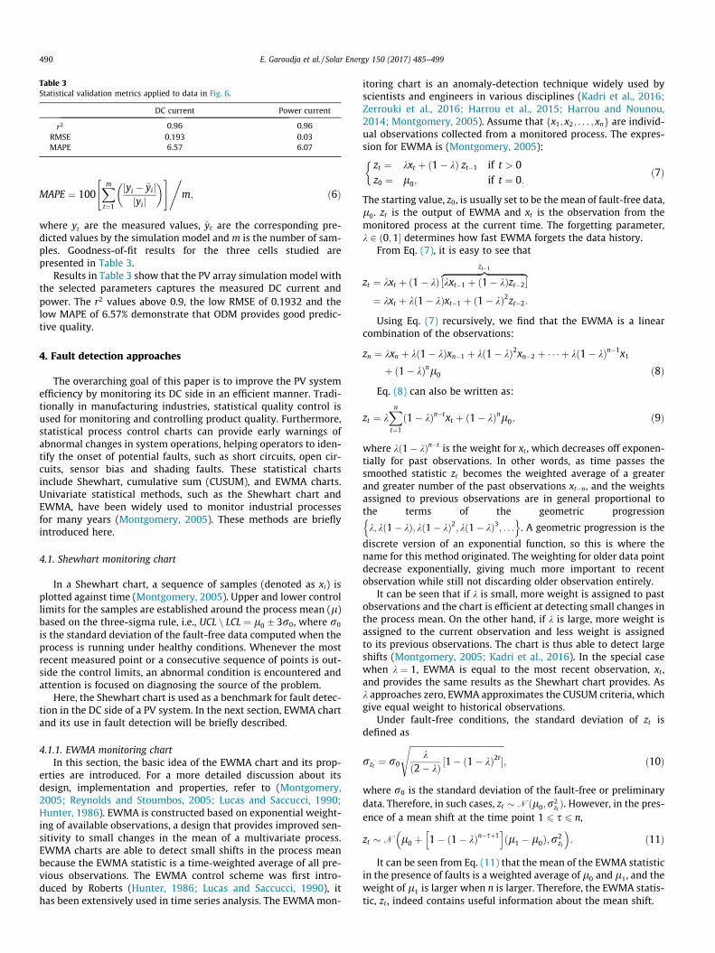
Table 3Statistical validation metrics applied to data in Fig. 6.

DC current Power current

r2 0.96 0.96RMSE 0.193 0.03MAPE 6.57 6.07

490 E. Garoudja et al. / Solar Energy 150 (2017) 485–499

MAPE ¼ 100Xmt¼1

jyi � yijjyij

� �" #,m; ð6Þ

where yt are the measured values, yt are the corresponding pre-dicted values by the simulation model and m is the number of sam-ples. Goodness-of-fit results for the three cells studied arepresented in Table 3.

Results in Table 3 show that the PV array simulation model withthe selected parameters captures the measured DC current andpower. The r2 values above 0.9, the low RMSE of 0.1932 and thelow MAPE of 6.57% demonstrate that ODM provides good predic-tive quality.

4. Fault detection approaches

The overarching goal of this paper is to improve the PV systemefficiency by monitoring its DC side in an efficient manner. Tradi-tionally in manufacturing industries, statistical quality control isused for monitoring and controlling product quality. Furthermore,statistical process control charts can provide early warnings ofabnormal changes in system operations, helping operators to iden-tify the onset of potential faults, such as short circuits, open cir-cuits, sensor bias and shading faults. These statistical chartsinclude Shewhart, cumulative sum (CUSUM), and EWMA charts.Univariate statistical methods, such as the Shewhart chart andEWMA, have been widely used to monitor industrial processesfor many years (Montgomery, 2005). These methods are brieflyintroduced here.

4.1. Shewhart monitoring chart

In a Shewhart chart, a sequence of samples (denoted as xi) isplotted against time (Montgomery, 2005). Upper and lower controllimits for the samples are established around the process mean (l)based on the three-sigma rule, i.e., UCL n LCL ¼ l0 � 3r0, where r0

is the standard deviation of the fault-free data computed when theprocess is running under healthy conditions. Whenever the mostrecent measured point or a consecutive sequence of points is out-side the control limits, an abnormal condition is encountered andattention is focused on diagnosing the source of the problem.

Here, the Shewhart chart is used as a benchmark for fault detec-tion in the DC side of a PV system. In the next section, EWMA chartand its use in fault detection will be briefly described.

4.1.1. EWMA monitoring chartIn this section, the basic idea of the EWMA chart and its prop-

erties are introduced. For a more detailed discussion about itsdesign, implementation and properties, refer to (Montgomery,2005; Reynolds and Stoumbos, 2005; Lucas and Saccucci, 1990;Hunter, 1986). EWMA is constructed based on exponential weight-ing of available observations, a design that provides improved sen-sitivity to small changes in the mean of a multivariate process.EWMA charts are able to detect small shifts in the process meanbecause the EWMA statistic is a time-weighted average of all pre-vious observations. The EWMA control scheme was first intro-duced by Roberts (Hunter, 1986; Lucas and Saccucci, 1990), ithas been extensively used in time series analysis. The EWMAmon-

itoring chart is an anomaly-detection technique widely used byscientists and engineers in various disciplines (Kadri et al., 2016;Zerrouki et al., 2016; Harrou et al., 2015; Harrou and Nounou,2014; Montgomery, 2005). Assume that fx1; x2; . . . ; xng are individ-ual observations collected from a monitored process. The expres-sion for EWMA is (Montgomery, 2005):

zt ¼ kxt þ 1� kð Þ zt�1 if t > 0z0 ¼ l0; if t ¼ 0:

�ð7Þ

The starting value, z0, is usually set to be the mean of fault-free data,l0. zt is the output of EWMA and xt is the observation from themonitored process at the current time. The forgetting parameter,k 2 ð0;1� determines how fast EWMA forgets the data history.

From Eq. (7), it is easy to see that

zt ¼ kxt þ 1� kð Þ kxt�1 þ 1� kð Þzt�2½ �zfflfflfflfflfflfflfflfflfflfflfflfflfflfflfflfflffl}|fflfflfflfflfflfflfflfflfflfflfflfflfflfflfflfflffl{zt�1

¼ kxt þ kð1� kÞxt�1 þ ð1� kÞ2zt�2:

Using Eq. (7) recursively, we find that the EWMA is a linearcombination of the observations:

zn ¼ kxn þ kð1� kÞxn�1 þ kð1� kÞ2xn�2 þ � � � þ kð1� kÞn�1x1

þ ð1� kÞnl0 ð8ÞEq. (8) can also be written as:

zt ¼ kXnt¼1

ð1� kÞn�txt þ ð1� kÞnl0; ð9Þ

where kð1� kÞn�t is the weight for xt , which decreases off exponen-tially for past observations. In other words, as time passes thesmoothed statistic zt becomes the weighted average of a greaterand greater number of the past observations xt�n, and the weightsassigned to previous observations are in general proportional tothe terms of the geometric progression

k; kð1� kÞ; kð1� kÞ2; kð1� kÞ3; . . .n o

. A geometric progression is the

discrete version of an exponential function, so this is where thename for this method originated. The weighting for older data pointdecrease exponentially, giving much more important to recentobservation while still not discarding older observation entirely.

It can be seen that if k is small, more weight is assigned to pastobservations and the chart is efficient at detecting small changes inthe process mean. On the other hand, if k is large, more weight isassigned to the current observation and less weight is assignedto its previous observations. The chart is thus able to detect largeshifts (Montgomery, 2005; Kadri et al., 2016). In the special casewhen k ¼ 1, EWMA is equal to the most recent observation, xt ,and provides the same results as the Shewhart chart provides. Ask approaches zero, EWMA approximates the CUSUM criteria, whichgive equal weight to historical observations.

Under fault-free conditions, the standard deviation of zt isdefined as

rzt ¼ r0

ffiffiffiffiffiffiffiffiffiffiffiffiffiffiffiffiffiffiffiffiffiffiffiffiffiffiffiffiffiffiffiffiffiffiffiffiffiffiffiffiffiffiffiffiffik

ð2� kÞ ½1� ð1� kÞ2t �s

; ð10Þ

where r0 is the standard deviation of the fault-free or preliminarydata. Therefore, in such cases, zt Nðl0;r2

zt Þ. However, in the pres-ence of a mean shift at the time point 1 6 s 6 n,

zt N l0 þ 1� ð1� kÞn�sþ1h i

ðl1 � l0Þ;r2zt

�: ð11Þ

It can be seen from Eq. (11) that the mean of the EWMA statisticin the presence of faults is a weighted average of l0 and l1, and theweight of l1 is larger when n is larger. Therefore, the EWMA statis-tic, zt , indeed contains useful information about the mean shift.

E. Garoudja et al. / Solar Energy 150 (2017) 485–499 491

The upper and lower control limits of the EWMA chart fordetecting a mean shift are

UCL=LCL ¼ l0 � Lrzt ; ð12Þwhere L is a multiplier of the EWMA standard deviation, rzt . Theparameters L and k need to be set carefully (Montgomery, 2005;Kadri et al., 2016). L is usually specified in practice to be 3, whichcorresponds to a false alarm rate of 0.27% implying that 99.73% ofthe observations should be contained within the control limits innormal conditions. The value of k is usually set between 0.2 and0.3 (Montgomery, 2005). On the other hand, from Eq. (10), it can

be seen that the term ½1� ð1� kÞ2t � converges to unity as t gets lar-ger. In practice people often use the asymptotic variance ofzt; ~r2

zt ¼ k2�k r

20. Of course, If zt is within the [LCL UCL] interval, then

it will be concluded that the process is under control up to timepoint t. Otherwise, the process is considered out of control.

4.2. ODM-based EWMA for PV monitoring

In general, the model is first built and then fault diagnosis pro-cedures is performed accordingly. The estimation of the residuals,which is crucial in model-based fault detection, depends on theappropriate system modeling. Once ODM is built based on datarepresenting historically normal operations and validated, it canbe used to monitor future deviations in the system. Here, theadvantages of ODM with those of the EWMA monitoring chartare combined, which should result in an improved fault detectionsystem, especially for detecting small changes. Specifically, in thisapproach, the EWMA chart is employed for fault detection to indi-cate how well the measurements conform to the model or howlarge the deviation from the normal model is. Towards this end,the EWMA chart is applied to monitor residuals obtained fromODM (see Fig. 7).

The differences between the real measured and predicted MPPcurrent, MPP voltage and MPP power obtained from the simulatedmodel are the residuals that can be used as indicators to detect apossible fault.

eIt ¼ It �bIt; eV t ¼ Vt � bV t ; ePt ¼ Pt � bPt ; t 2 ½1;n�; ð13Þ

where It and bIt are the measured and predicted MPP current,

respectively, and Vt and bV t are the measured and predicted MPP

voltage; and Pt and bPt are the measured and predicted peak power.In this work, the residuals are used as fault indicators. Indeed, under

Fig. 7. A flowchart of the propo

normal operation, the residuals are close to zero due to measure-ment noise and errors, while they significantly deviate from zeroin the presence of abnormal events. The implementation of thedeveloped monitoring methods comprises two stages: off-line mod-eling and on-line monitoring. In the off-line modeling phase, ODMis used on the normal operating data (training data), enabling usto obtain a reference model. Then, the fault detection procedure isexecuted by using the reference simulated model with the EWMAchart in the on-line monitoring phase. The ODM-EWMA fault detec-tion algorithm is summarized in Table 4.

To improve system operations, we want not only to monitor thesystem in an efficient manner but also to identify the type of faultthat results in any degradation of the PV system, including declinesin operation reliability, and profitability, such that we can respondaccordingly by making any necessary correction to the system.Towards this end, the EWMA chart is applied based on the residualof output DC power to detect the presence of faults. Then, the typeof fault is identified by analyzing the monitoring results of theEWMA chart when it is applied to the residuals of output DC cur-rent and voltage. The fault identification procedure is summarizedin Fig. 8.

The proposed strategy tests at the first stage the peak power todetect a fault. This choice is mainly due to the fact that faults affectinevitably the peak power. Thus, the peak power is used as a faultindicator in the detection phase. On the other hand, both DC outputcurrent and voltage are unsuitable to be used as sensitive indica-tors in this phase. For example, when a short circuit occurs inone PV module from a string, current indicator value will not besignificantly changed from its healthy set point. Meanwhile, a sub-stantial change will appear in the power indicator (peak of power).Besides, the same situation occurs when a string is completely dis-connected. Indeed, the DC output voltage remains unalteredregarding its healthy status in contrast to the peak power decreasesignificantly. Moreover, the ranking of the current and voltageindicators is unimportant in the fault diagnosis phase.

5. Results and discussion

5.1. Detection results

The proposed fault detection scheme is validated using practicaldata collected from the 9.54 kWp GCPV system installed at CDER inAlgeria (see Section 2). In this section, the ability of the EWMAchart to detect the presence of faults in the data and to identify

sed fault detection scheme.

Table 4EWMA-based fault detection algorithm for PV system monitoring.

(1) Given Real measurement of irradiance and module temperature Real measurement of maximum power point (MPP) values of current, voltage and power collected from the PV plant under normal operating conditions Module parameters obtained from the PV module datasheet (see Table 1)

(2) Build ODM using the fault-free training data Extract electrical parameters for the five-parameter model based on the measured cell temperature and irradiance collected from the monitored PV system

under normal operating conditions (see Section 2) using the Artificial Bee Colony (ABC) algorithm (Garoudja et al., 2015). The extracted parameters are thenused to simulate the PV system

Compute the residuals between the measured and the predicted DC current, DC voltage and DC power (Impp;Vmpp and Pmpp) from the constructed modelusing fault-free data

Compute the control limits for the EWMA chart using Eq. (12)(3) Test the new data

Generate residual vectors, eI; eV and eP , using the selected five-parameter-based model Compute the EWMA monitoring statistic for the new data using Eq. (7)

(4) Check for faults Declare a fault when the EWMA decision statistic for the new data exceeds the control limits

Fig. 8. Fault identification procedure.

492 E. Garoudja et al. / Solar Energy 150 (2017) 485–499

the type of detected fault is assessed. To assess the strength of theEWMA-based monitoring chart, three case studies involving differ-ent types of faults were conducted. In the first case study, it isassumed that the PV system contains one or more short-circuitedPV module (case A). In the second case study, an open-circuit PVstring is considered (case B). In the third case study, the monitoredPV system is exposed to temporary shadowing (case C).

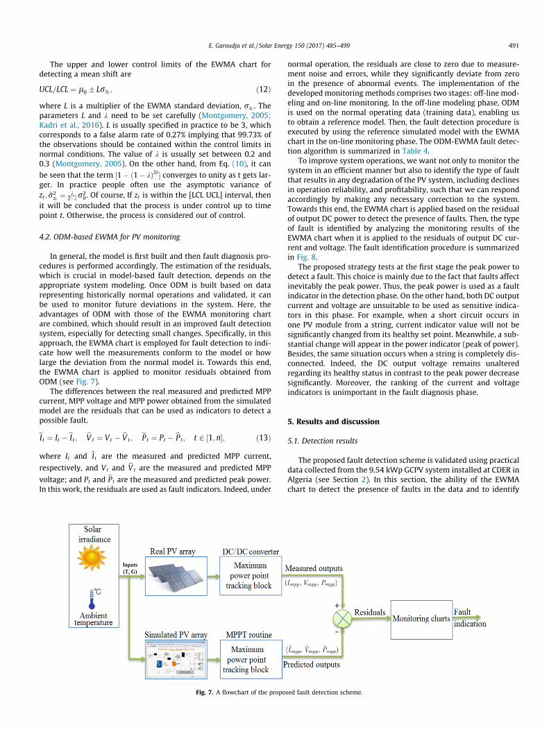
5.1.1. Normal operating conditionsMonitoring results from ODM-based Shewhart chart under nor-

mal operating conditions are shown in Fig. 9(a)–(c), monitoringresults from the EWMA chart under normal operating conditionsare presented in Fig. 10(a)–(c). Since the Shewhart plots for cur-rent, voltage and power shown in Fig. 9(a)–(c) are based on normaloperating data, we expect that almost all the data will lie withinthe lower and upper control limits. Similarly, the data points inthe EWMA charts are also within the 95% confidence limits (seeFig. 10(a)–(c)). It can be concluded that the ODM model describesthe data well when no faults are present.

5.1.2. Case study of open-circuit PV stringsIn this case study, the performance of the twomonitoring charts

when there is an open-circuit fault is investigated. To do so, anopen-circuit fault in a PV array is introduced by disconnectingthe second string from the monitored PV system (see fault #1 inFig. 11) between sample times 300–500.

To monitor the PV system, the residuals (i.e., eI; eV and eP) are firstcomputed. Then both monitoring charts, Shewhart and EWMA, areused for fault detection. The Shewhart and EWMA charts based onthe MPP residuals of current, voltage and power are presented inFigs. 12 and 13, respectively. The shaded area is the region wherethe fault is introduced. The plots in Figs. 12(c) and 13(c) indicatethat before the occurrence of the fault, both charts are within thelower and upper control limits. The PV system is thus working nor-mally. For this case, the two charts can both give fault signalsbecause the introduced fault is quite large. Figs. 12(c) and 13(c),show that the Shewhart and EWMA charts based on the output

power residuals, eP , decrease significantly and exceed the lowercontrol limits, indicating that there is a significant power loss.

0 100 200 300 400 500−0.2

−0.1

0

0.1

0.2

Observation Number

DC

cur

rent

resi

dual

s

(a)

0 100 200 300 400 500−0.2

−0.1

0

0.1

0.2

0.3

Observation Number

DC

vol

tage

resi

dual

s

(b)

UCL\LCL

0 100 200 300 400 500−0.1

−0.05

0

0.05

0.1

Observation Number

DC

pow

er re

sidu

als

(c)

UCL\LCLUCL/LCL

Fig. 9. Monitoring results of a Shewhart chart for DC current (a), DC voltage (b) and DC power (c) under normal operating conditions.

0 100 200 300 400 500−0.2

−0.1

0

0.1

0.2

Observation number

EWM

A st

atis

tic

(a)

UCL/LCL

0 100 200 300 400 500−0.1

0

0.1

0.2

0.3

Observation number

EW

MA

sta

tistic

(b)

UCL/LCL

0 100 200 300 400 500−0.05

0

0.05

0.1

0.15

Observation number

EWM

A st

atis

tic

(c)

UCL/LCL

Fig. 10. Monitoring results of EWMA chart for DC current (a), DC voltage (b) and DC power (c) under normal operating conditions.

Fig. 11. Open-circuit and short-circuit faults.

E. Garoudja et al. / Solar Energy 150 (2017) 485–499 493

Since one of the two strings of a PV array is disconnected at thefault, a large amount of power (nearly 50% of the rated power) islost. After detecting the presence of a fault, the monitoring resultsrelated to the output DC current and voltage are analyzed to iden-tify the type of fault. Both Figs. 12(b) and 13(b) are within thelower and upper control limits before and after the fault, which

means that the DC voltage is almost the same after the occurrenceof this open-circuit fault. The two monitoring charts based on thecurrent residuals are given in Figs. 12(a) and 13(a). These chartsshow that both charts exceed the lower control limits, indicatingthe presence of a faulty string (open-circuit fault). Indeed, the cur-rent of the faulty string drops to zero when the string is discon-

0 100 200 300 400 500

−1

−0.5

0

Observation Number

DC

cur

rent

resi

dual

s

(a)

UCL\LCL

0 100 200 300 400 500

−0.2

−0.1

0

0.1

0.2

Observation Number

DC

vol

tage

resi

dual

s

(b)

UCL\LCL

0 100 200 300 400 500

−1

−0.5

0

Observation Number

DC

pow

er re

sidu

als

(c)

UCL\LCL

Fig. 12. Monitoring results of a Shewhart chart for DC current (a), DC voltage (b) and DC power (c) in the presence of an open-circuit fault.

Observation number

EWM

A st

atis

tic

-1

-0.5

0

(a)

UCL\LCL

Observation number

EWM

A st

atis

tic

-0.1

0

0.1

0.2

0.3(b)

UCL\LCL

Observation number

EWM

A st

atis

tic

-1

-0.5

0

(c)

UCL\LCL

0 100 200 300 400 500 0 100 200 300 400 500 0 100 200 300 400 500

Fig. 13. Monitoring results of an EWMA chart for DC current (a), DC voltage (b) and DC power (c) in the presence of an open-circuit fault.

494 E. Garoudja et al. / Solar Energy 150 (2017) 485–499

nected from the PV array. As a result, the residuals, which indicatethe difference between the simulated and measured DC current,decrease immediately after the occurrence of the open-circuitfault. From this case study, it can be seen that the open-circuit faultin a PV array increases the power loss, reduces the array currentand results in almost the same array voltage as the normal PV arrayvoltage. These results indicate the efficiency of both fault detectionstrategies in detecting and diagnosing open-circuit faults in a PVsystem.

5.1.3. Case study of a short circuit in a string of PV modulesIn this case study, the detection of short-circuited PV modules

in the monitored PV system is investigated. Four examples aregiven in this case study (see Fig. 11, faults #2–#5).

(1) One short-circuited PV module: In the first example, the sec-ond module of the first string is bypassed from observation num-ber 300 until the end of the testing data (see Fig. 11, fault #2).The output DC current, voltage and power were monitored usingShewhart and EWMA charts. The two monitoring charts are shownin Fig. 14(a)–(c) and Fig. 15(a)–(c). Fig. 14 shows that the Shewhartchart cannot detect this fault. The Shewhart chart is insensitive tothis fault because it is designed to detect relatively moderate andlarge faults, while the fault in this case is quite small. This is mainly

0 100 200−0.2

−0.1

0

0.1

0.2

0.3

Observatio

DC

vol

tage

resi

dual

s

UCL\

0 100 200 300 400 500

−0.1

0

0.1

Observation Number

DC

cur

rent

resi

dual

s

(a)

UCL\LCL

Fig. 14. Monitoring results of a Shewhart chart for DC current (a), DC volta

due to the fact that the Shewhart chart uses only observed data at aparticular instant to make a decision about the process perfor-mance and it ignores past data. On the other hand, the plot inFig. 15(c) clearly shows the capability of the EWMA monitoringchart in detecting this small fault. From the plots in Fig. 15(a)and (b), it can be seen that the DC current residuals are withinthe control limits, while the DC voltage residuals exceeds the lowercontrol limit. Thus, we can conclude that the detected fault isrelated to a faulty module in the string. This case study clearlyshows the superiority of the EWMA over the Shewhart chart indetecting small faults.

(2) Three short-circuited PV modules: In the second example,three modules have been short circuited in the first string (seeFig. 11, fault #3). The monitoring results of the Shewhart andEWMA charts are shown in Figs. 16 and 17, respectively. The per-formance of the Shewhart chart when it is applied to the outputpower residuals is presented in Fig. 16(c), which shows that theShewhart statistic clearly violates the lower control limit. The She-whart chart detects this fault (i.e., a power loss) but it misses somedata. On the other hand, the plot in Fig. 17(c) clearly shows thecapability of the EWMA monitoring chart in correctly detectingthis moderate fault without missed data. This short-circuit faultdegrades the performance of the monitored systems and leads to

300 400 500

n Number

(b)

LCL

0 100 200 300 400 500−0.1

−0.05

0

0.05

0.1

Observation Number

DC

pow

er re

sidu

als

(c)

UCL\LCL

ge (b) and DC power (c) in the presence of one short-circuited module.

0 100 200 300 400 500

−0.1

0

0.1

Observation Number

DC

cur

rent

resi

dual

s

(a)

UCL/LCL

0 100 200 300 400 500

−0.4

−0.2

0

0.2

Observation Number

DC

vol

tage

resi

dual

s

(b)

UCL/LCL

0 100 200 300 400 500

−0.2

−0.1

0

0.1

Observation Number

DC

pow

er re

sidu

als (c)

UCL/LCL

Missed detections

Fig. 16. Monitoring results of a Shewhart chart for DC current (a), DC voltage (b) and DC power (c) in the presence of three short-circuited modules in a PV array.

Observation number

EWM

A st

atis

tic

-0.2

-0.1

0

0.1

0.2(a)

LCL/UCL

Observation number

EWM

A st

atis

tic

-0.4

-0.2

0

0.2(b)

LCL/UCL

Observation number

EWM

A st

atis

tic

-0.2

-0.1

0

0.1(c)

LCL/UCL

0 100 200 300 400 500 0 100 200 300 400 500 0 100 200 300 400 500

Fig. 17. Monitoring results of an EWMA chart for DC current (a), DC voltage (b) and DC power (c) in the presence of three short-circuited modules in a PV array.

0 100 200 300 400 500

−0.1

0

0.1

0.2

Observation Number

EW

MA

sta

tistic

(b)

UCL\LCL

0 100 200 300 400 500

−0.05

0

0.05

Observation Number

EW

MA

sta

tistic

(c)

UCL\LCL

0 100 200 300 400 500−0.2

−0.1

0

0.1

0.2

Observation number

EWM

A st

atis

tic

(a)

UCL/LCL

Fig. 15. Monitoring results of an EWMA chart for DC current (a), DC voltage (b) and DC power (c) in the presence of one short-circuited module.

E. Garoudja et al. / Solar Energy 150 (2017) 485–499 495

a significant power loss (i.e., approximatively 15% power loss).After detecting a fault based on the output DC power, the twomon-itoring charts based on residuals of output DC current and voltage,which are shown in Figs. 16(a) and (b) and 17(a) and (b), can pro-vide more information about the type of fault. Both Figs. 16(b) and17(b) show fault signals because the decrease in output DC voltagein this case is quite large. The output DC current from the arraydoes not change by much. Because the output DC voltage decreasescompared to the output DC voltage of the normal array and the

0 100 200 300 400 500

−0.1

0

0.1

Observation Number

DC

cur

rent

resi

dual

s

(a)

UCL\LCL

0 100 200−0.9

−0.25

0.4

Observation

DC

vol

tage

resi

dual

s

(

UCL\L

Fig. 18. Monitoring results of a Shewhart chart for DC current (a), DC voltage (b) a

output DC current does not change by much, we then concludethat this fault is a short circuit in the PV array.

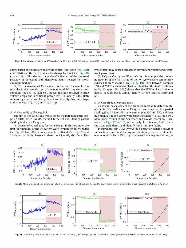
(3) Five short-circuited PV modules: In the third example, fivemodules in first string are disconnected (Fig. 11, fault #4). Thisfault leads to a power loss of 30% compared to the healthy PV array.Both monitoring charts can detect this quite large fault as shown inFigs. 18(c) and 19(c). Similar to the cases above, to identify thisfault, we look at the monitoring results related to the array voltageand current (see Figs. 18(a) and (b) and 19(a) and (b)). In fact, it is afault that corresponds to a short-circuited PV module, since both

300 400 500

Number

b)

CL

0 100 200 300 400 500

−0.6

−0.4

−0.2

0

0.2

Observation Number

DC

pow

er re

sidu

als

(c)

UCL\LCL

nd DC power (c) in the presence of five short-circuited modules in a PV array.

Observation number

EWM

A st

atis

tic

-0.2

-0.1

0

0.1

0.2(a)

ULC/LCL

Observation number

EWM

A st

atis

tic

-0.8

-0.6

-0.4

-0.2

0

0.2

(b)

ULC/LCL

Observation number

EWM

A st

atis

tic

-0.6

-0.4

-0.2

0

0.2(c)

ULC/LCL

0 100 200 300 400 500 0 100 200 300 400 500 0 100 200 300 400 500

Fig. 19. Monitoring results of an EWMA chart for DC current (a), DC voltage (b) and DC power (c) in the presence of five short-circuited modules in a PV array.

496 E. Garoudja et al. / Solar Energy 150 (2017) 485–499

charts based on voltage are below the control limits (see Figs. 18(b)and 19(b)), and the current does not change by much (see Figs. 18(a) and 19(a)). This demonstrates the effectiveness of the proposedstrategy in detecting and identifying faults related to short-circuited modules.

(4) Ten short-circuited PV modules: In the fourth example, tenmodules in the second string of the monitored PV array were shortcircuited (see Fig. 11, fault #5). Indeed, the fault resulted in largevoltage drops and significant power loss (i.e. nearly 63%). Bothmonitoring charts can clearly detect and identify this quite largefault (see Figs. 20(a)–(c) and 21(a)–(c)).

5.1.4. Case study of shading faultThe aim of this case study was to assess the potential of the pro-

posed ODM-based EWMA method to detect and identify partialshading faults in a PV system.

(1) Temporarily shading of four PV modules: In this example, thefirst four modules of the PV system were temporarily fully shaded(see Fig. 22, fault #6), between samples 150 and 250. Figs. 23 and24 show that both charts can detect and identify this fault. This

0 100 200 300 400 500

−0.1

−0.05

0

0.05

0.1

0.15

Observation Number

DC

cur

rent

resi

dual

s

(a)

UCL/LCL

0 100 200−2

−1.5

−1

−0.5

0

Observatio

DC

vol

tage

resi

dual

s

UCL\L

Fig. 20. Monitoring results of a Shewhart chart for DC current (a), DC voltage (b) a

Observation number

EWM

A st

atis

tic

-0.2

-0.1

0

0.1

0.2(a)

UCL\LCL

Observatio

EWM

A st

atis

tic

-2

-1.5

-1

-0.5

0

(

UCL\LC

0 100 200 300 400 500 0 100 200

Fig. 21. Monitoring results of an EWMA chart for DC current (a), DC voltage (b) an

type of fault may cause decreases in current and voltage and signif-icant power loss.

(2) Fully shading of one PV module: In this example, the modulenumber 14 of the first string of the PV system were temporarilyexposed to fully shading (see Fig. 22, fault #7), between samples150 and 250. The shewhart chart fails to detect this fault, as shownin Fig. 25(a)–(c). Fig. 26(c) shows that the EWMA chart is able todetect the fault, but it cannot identify its type (see Fig. 26(b) and(c)).

5.1.5. Case study of multiple faultsTo assess the capacity of the proposed method to detect multi-

ple faults, five modules in the PV system were exposed to a partialshading (Fig. 22, fault #6), between samples 150 and 250, and thenfive modules in one string were short-circuited (Fig. 22, fault #8).Monitoring results of the Shewhart and EWMA charts are illus-trated in Figs. 27 and 28, respectively. In this case, both chartscan accurately detect and identify these multiple faults.

In summary, our ODM-EWMA fault detection scheme providessatisfactory results in detecting and identifying short-circuit faults,open-circuit faults in PV strings and partial shading. In addition, to

300 400 500

n Number

(b)

CL

0 100 200 300 400 500−1.5

−1

−0.5

0

Observation Number

DC

pow

er rs

idua

ls

(c)

UCL\LCL

nd DC power (c) in the presence of ten short-circuited modules in a PV array.

n number

b)

L

Observation number

EWM

A st

atis

tic

-1.5

-1

-0.5

0

(c)

UCL\LCL

300 400 500 0 100 200 300 400 500

d DC power (c) in the presence of ten short-circuited modules in a PV array.

0 100 200 300 400 500−0.4

−0.2

0

0.2

Observation Number

DC

cur

rent

resi

dual

s

(a)

UCL/LCL0 100 200 300 400 500

−0.2

0

0.2

Observation Number

DC

vol

tage

resi

dual

s

(b)

UCL/LCL

0 100 200 300 400 500

−0.4

−0.2

0

0.2

Observation Number

DC

pow

er re

sidu

als

(c)

UCL/LCL

Fig. 23. Monitoring results of Shewhart chart for DC current (a), DC voltage (b) and DC power (c) in the presence of 4 PV modules temporarily shaded in the PV system.

0 100 200 300 400 500−0.4

−0.2

0

0.2

Observation number

EWM

A st

atis

tic

(a)

UCL/LCL0 100 200 300 400 500

−0.4

−0.2

0

0.2

Observation number

EWM

A st

atis

tic

(b)

UCL/LCL

0 100 200 300 400 500

−0.6

−0.4

−0.2

0

0.2

Observation number

EWM

A st

atis

tic

(c)

UCL/LCL

Fig. 24. Monitoring results of EWMA chart for DC current (a), DC voltage (b) and DC power (c) in the presence of 4 PV modules temporarily shaded in the PV system.

Fig. 22. Typical faults in a PV array: temporarily shading and faulty modules.

Observation Number

-0.2

-0.1

0

0.1

0.2

Res

idua

ls c

urre

nt

(a)

UCL\LCL

Observation Number

-0.2

0

0.2

0.4

Res

idua

ls v

olta

ge

(b)UCL\LCL

Observation Number

-0.1

0

0.1

Res

idua

ls p

ower

(c)UCL\LCL

0 100 200 300 400 0 100 200 300 400 500 0 100 200 300 400 500

Fig. 25. Monitoring results of Shewhart chart for DC current (a), DC voltage (b) and DC power (c) in the presence of 4 PV modules fully shaded in the PV system.

E. Garoudja et al. / Solar Energy 150 (2017) 485–499 497

0 100 200 300 400 500−0.4

−0.2

0

0.2

Observation Number

DC

cur

rent

resi

dual

s

(a)

UCL/LCL

0 100 200 300 400 500

−0.8

−0.6

−0.4

−0.2

0

0.2

Observation Number

DC

vol

tage

resi

dual

s (b)

UCL\LCL

0 100 200 300 400 500

−0.6

−0.4

−0.2

0

Observation Number

DC

pow

er re

sidu

als

(c)

UCL/LCL

Fig. 27. Monitoring results of a Shewhart chart for DC current (a), DC voltage (b) and DC power (c) in the presence of 4 PV modules that are partially shaded and five short-circuited modules in the PV system.

0 100 200 300 400 500

−0.3

−0.2

−0.1

0

0.1

0.2

Observation number

EWM

A st

atis

tic

(a)

UCL/LCL

0 100 200 300 400 500−0.8

−0.6

−0.4

−0.2

0

0.2

Observation number

EWM

A st

atis

tic

(b)

UCL\LCL

0 100 200 300 400 500

−0.6

−0.4

−0.2

0

Observation number

EWM

A st

atis

tic(c)

UCL/LCL

Fig. 28. Monitoring results of an EWMA chart for DC current (a), DC voltage (b) and DC power (c) in the presence of4 PV modules that are partially shaded and five short-circuited modules in the PV system.

Observation Number

-0.2

-0.1

0

0.1

0.2

EW

MA

sta

tistic

(a)

UCL\LCL

Observation Number

-0.2

0

0.2

0.4

EW

MA

sta

tistic

(b)UCL\LCL

Observation Number

-0.1

-0.05

0

0.05

0.1

EW

MA

sta

tistic

(c)UCL\LCL

0 100 200 300 400 500 0 100 200 300 400 500 0 100 200 300 400 500

Fig. 26. Monitoring results of EWMA chart for DC current (a), DC voltage (b) and DC power (c) in the presence of one PV module fully shaded in the PV system.

498 E. Garoudja et al. / Solar Energy 150 (2017) 485–499

detect small changes (e.g., one short-circuited module in a string),the EWMA chart is more effective.

6. Conclusion

Solar-energy-based photovoltaic (PV) systems are increasinglygaining worldwide attention due to the high electricity consump-tion in combination with the desired environmental friendly solu-tions for power production development. Indeed, PV systems arecontinuously exposed to many factors that significantly degradetheir performances and efficiency. Faults such as short-circuit,open circuit and shading in PV systems can reduce solar energyproductivity, leading to economic losses. This paper reports thedevelopment of a statistical fault detection approach for monitor-ing the performances of PV systems by detecting faults on the DCside and diagnosing the type of detected fault. This approach usesa simulation model based on the extracted ODMmodel parametersto predict the maximum current, voltage and power generatedfrom the PV system. Residuals, which are the difference betweenmeasured and predicted variables, are used as input for the EWMA

chart. Then, the EWMA based on residuals of output DC power isused to identify, in real time, the presence of faults in the moni-tored system. Voltage and current residuals are used to differenti-ate between open-circuit faults, short-circuit faults and partialshading in a PV system. Using practical data from a grid-connected PV system at CDER in Algeria, the effectiveness ofODM-EWMA to detect and identify faults in an actual PV systemhas been demonstrated.

Despite the promising results for fault detection and diagnosisobtained using the ODM-EWMA approach, the work carried outin this paper raises a number of question and provides some direc-tions for future works. In particular, the following points meritconsideration from researchers.

Beside fault detection and diagnosis capability, the EWMA chartis able to capture fault severity (amplitude). The larger the faultis, the greater the amplitude of the EWMA statistic compared toits amplitude under healthy conditions. Therefore, thisapproach can be extended to determine the number of faultyPV strings and/or PV modules.

E. Garoudja et al. / Solar Energy 150 (2017) 485–499 499

Herein, the diagnosis of the fault is done on the basis of only theMPP coordinates of current and voltage to identify the type offault. In fact, the shading of one PV module or small portionof PV module does not necessarily affect simultaneously currentand voltage MPP coordinates. Hence the proposed diagnosismethod cannot correctly discriminate this fault. To bypass thisshortcoming, we plan to include more input data such as opencircuit voltage (Voc), short circuit current (Isc) and fill factor(FF) since they are affected significantly by shading fault.

The presence of noisy and correlated data makes the faultdetection more difficult as the presence of noise degrades faultdetection quality and most methods are developed for indepen-dent observations. In fact, wavelet-based multiscale representa-tion of data has been shown to provide effective noise-featureseparation in the data and to approximately decorrelate theauto-correlated data. As future work, the aim is to develop mul-tiscale EWMA fault detection methods that can provideenhanced performances of this technique, especially when dataobserved from PV system are noisy and highly autocorrelated.

Acknowledgement

We would like to thank the reviewers of this article for theirinsightful comments, which helped us to greatly improve its qual-ity. This publication is based upon work supported by King Abdul-lah University of Science and Technology (KAUST), Office ofSponsored Research (OSR) under Award No: OSR-2015-CRG4-2582. The authors (Elyes Garoudja and Kamel Kara) thank theSET Laboratory, Department of Electronics, Faculty of Technology,University of Blida 1, Algeria, for continuous support during thestudy.

References

Abou, S., Chouder, A., Kara, K., Silvestre, S., 2015. Artificial bee colony basedalgorithm for maximum power point tracking (MPPT) for PV systems operatingunder partial shaded conditions. Appl. Soft Comput. 32, 38–48.

Alam, M., Khan, F., Johnson, J., Flicker, J., 2015. A comprehensive review ofcatastrophic faults in PV arrays: types, detection, and mitigation techniques.IEEE J. Photovoltaics 5 (3), 982–997.

Arab, A., Cherfa, F., Chouder, A., Chenlo, F., 2005. Grid-connected photovoltaicsystem at CDER-algeria. In: 20th European Photovoltaic Solar EnergyConference and Exhibition, Barcelone, pp. 6–10.

Brooks, B., 2011. The bakersfield fire: a lesson in ground-fault protection. SolarPro 4(2).

Chao, K., Ho, S., Wang, M., 2008. Modeling and fault diagnosis of a photovoltaicsystem. Electr. Power Syst. Res. 78 (1), 97–105.

Chine, W., Mellit, A., Lughi, V., Malek, A., Sulligoi, G., Pavan, A., 2016. A novel faultdiagnosis technique for photovoltaic systems based on artificial neuralnetworks. Renew. Energy 90, 501–512.

Chouder, A., Silvestre, S., 2009. Analysis model of mismatch power losses in PVsystems. J. Sol. Energy Eng. 131 (2), 024504.

Chouder, A., Silvestre, S., 2010. Automatic supervision and fault detection of PVsystems based on power losses analysis. Energy Convers. Manage. 51 (10),1929–1937.

Duffie, J., Beckman, W., 2013. Solar Engineering of Thermal Processes, vol. 3. Wiley,New York.

Garoudja, E., Kara, K., Chouder, A., Silvestre, S., 2015. Parameters extraction ofphotovoltaic module for long-term prediction using artificial bee colonyoptimization. In: 3rd International Conference on Control, Engineering &Information Technology (CEIT). IEEE, pp. 1–6.

Hachana, O., Tina, G., Hemsas, K., 2016. PV array fault diagnostic technique for BIPVsystems. Energy Build. 126, 263–274.

Hare, J., Shi, X., Gupta, S., Bazzi, A., 2016. Fault diagnostics in smart micro-grids: asurvey. Renew. Sustain. Energy Rev. 60, 1114–1124.

Hariharan, R., Chakkarapani, M., Ilango, G., Nagamani, C., 2016. A method to detectphotovoltaic array faults and partial shading in PV systems. IEEE J. Photovoltaics6 (5), 1278–1285.

Harrou, F., Fillatre, L., Nikiforov, I., 2014. Anomaly detection/detectability for alinear model with a bounded nuisance parameter. Ann. Rev. Contr. 38 (1), 32–44.

Harrou, F., Nounou, M., 2014. Monitoring linear antenna arrays using anexponentially weighted moving average-based fault detection scheme. Syst.Sci. Contr. Eng.: Open Access J. 2 (1), 433–443.

Harrou, F., Nounou, M., Nounou, H., Madakyaru, M., 2015. PLS-based EWMA faultdetection strategy for process monitoring. J. Loss Prev. Process Ind. 36, 108–119.

Hu, Y., Cao, W., Wu, J., Ji, B., Holliday, D., 2014. Thermography-based virtual MPPTscheme for improving PV energy efficiency under partial shading conditions.IEEE Trans. Power Electron. 29 (11), 5667–5672.

Hunter, J.S., 1986. The exponentially weighted moving average. J. Qual. Technol. 18(4), 203–210.

Johansson, T., 1993. Renewable Energy: Sources for Fuels and Electricity. IslandPress.

Johnson, J., Kuszmaul, S., Bower, W., Schoenwald, D., 2011. Using PV module andline frequency response data to create robust arc fault detectors. In:Proceedings of the 26th European Photovoltaic Solar Energy Conference andExhibition, pp. 05–09.

Kadri, F., Harrou, F., Chaabane, S., Sun, Y., Tahon, C., 2016. Seasonal ARMA-based SPCcharts for anomaly detection: application to emergency department systems.Neurocomputing 173, 2102–2114.

Kang, B., Kim, S., Bae, S., Park, J., 2012. Diagnosis of output power lowering in a PVarray by using the Kalman-filter algorithm. IEEE Trans. Energy Convers. 27 (4),885–894.

Lucas, J., Saccucci, M., 1990. Exponentially weighted moving average controlschemes: properties and enhancements. Technometrics 32 (1), 1–12.

McEvoy, A., Castaner, L., Markvart, T., 2012. Solar Cells: Materials, Manufacture andOperation. Academic Press.

Mekki, H., Mellit, A., Salhi, H.H., 2016. Artificial neural network-based modellingand fault detection of partial shaded photovoltaic modules. Simul. Model. Pract.Theory 67, 1–13.

Montgomery, D., 2007. Introduction to Statistical Quality Control. John Wiley &Sons.

Montgomery, D.C., 2005. Introduction to Statistical Quality Control. John Wiley&Sons, New York.

Munoz, M., Alonso-Garcia, M., Vela, N., Chenlo, F., 2011. Early degradation of siliconPV modules and guaranty conditions. Sol. Energy 85 (9), 2264–2274.

Panwar, N., Kaushik, S., Kothari, S., 2011. Role of renewable energy sources inenvironmental protection: a review. Renew. Sustain. Energy Rev. 15 (3), 1513–1524.

Pavan, A., Mellit, A., Pieri, D., Kalogirou, S., 2013. A comparison between BNN andregression polynomial methods for the evaluation of the effect of soiling in largescale photovoltaic plants. Appl. Energy 108, 392–401.

Platon, R., Martel, J., Woodruff, N., Chau, T., 2015. Online fault detection in PVsystems. IEEE Trans. Sustain. Energy 6 (4), 1200–1207.

Reynolds, M., Stoumbos, Z., 2005. Should exponentially weighted moving averageand cumulative sum charts be used with Shewhart limits? Technometrics 47(4), 409–424.

Shrikhande, S., Varde, P., Datta, D., 2016. Prognostics and health management:methodologies & soft computing techniques. In: Current Trends in Reliability,Availability, Maintainability and Safety. Springer, pp. 213–227.

Silvestre, S., daSilva, M., Chouder, A., Guasch, D., Karatepe, E., 2014. New procedurefor fault detection in grid connected PV systems based on the evaluation ofcurrent and voltage indicators. Energy Convers. Manage. 86, 241–249.

Silvestre, S., Kichou, S., Chouder, A., Nofuentes, G., Karatepe, E., 2015. Analysis ofcurrent and voltage indicators in grid connected PV (photovoltaic) systemsworking in faulty and partial shading conditions. Energy 86, 42–50.

Suganthi, L., Iniyan, S., Samuel, A., 2015. Applications of fuzzy logic in renewableenergy systems – a review. Renew. Sustain. Energy Rev. 48, 585–607.

Tadj, M., Benmouiza, K., Cheknane, A., Silvestre, S., 2014. Improving theperformance of PV systems by faults detection using GISTEL approach. EnergyConvers. Manage. 80, 298–304.

Vergura, S., Acciani, G., Amoruso, V., Patrono, G., Vacca, F., 2009. Descriptive andinferential statistics for supervising and monitoring the operation of PV plants.IEEE Trans. Ind. Electron. 56 (11), 4456–4464.

Yahyaoui, I., Segatto, M., 2017. A practical technique for on-line monitoring of aphotovoltaic plant connected to a single-phase grid. Energy Convers. Manage.132, 198–206.

Zerrouki, N., Harrou, F., Sun, Y., Houacine, A., 2016. Accelerometer and camera-based strategy for improved human fall detection. J. Med. Syst. 40 (12), 284.

Zhao, Y., Ball, R., Mosesian, J., dePalma, J., Lehman, B., 2015. Graph-based semi-supervised learning for fault detection and classification in solar photovoltaicarrays. IEEE Trans. Power Electron. 30 (5), 2848–2858.

Zhao, Y., dePalma, J., Mosesian, J., Lyons, R., Lehman, B., 2013. Line–line faultanalysis and protection challenges in solar photovoltaic arrays. IEEE Trans. Ind.Electron. 60 (9), 3784–3795.