1

Monitoring and Fault Detection with Multivariate Statistical Process Control (MSPC) in

Continuous and Batch Processes

Barry M. Wise, Ph.D.Eigenvector Research, Inc.

Manson, WA

2

Outline• Definition of Chemometrics• Favorite tools

• Principal Components Analysis (PCA)• Partial Least Squares Regression (PLS)• Multi-way methods

• Opportunities in PAT• Multivariate Statistical Process Control (MSPC)• Image analysis on tablets• Predicting monitored or controlled variables• Batch MSPC

3

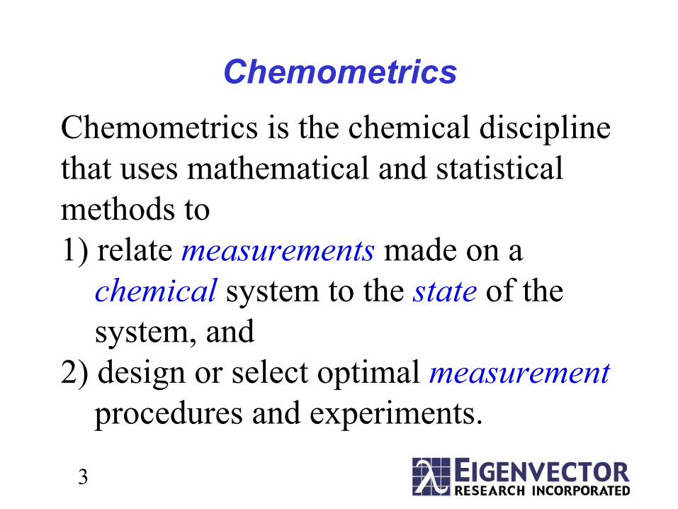
ChemometricsChemometrics is the chemical discipline that uses mathematical and statistical methods to1) relate measurements made on a

chemical system to the state of thesystem, and

2) design or select optimal measurementprocedures and experiments.

4

Multivariate Analysis

Multivariate Statistical Analysis is concerned with data that consists of

multiple measurements on a number of individuals, objects, or data samples.

The measurement and analysis of dependence between variables is

fundamental to multivariate analysis.

5

Multi-way Analysis

Multi-way Analysis is concerned withdata that is measured as a function of

three or more factors.

6

Multivariate Images

A data array of dimension three (ormore) where the first two dimensionsare spatial and the last dimension(s) is

a function of another variable.

7

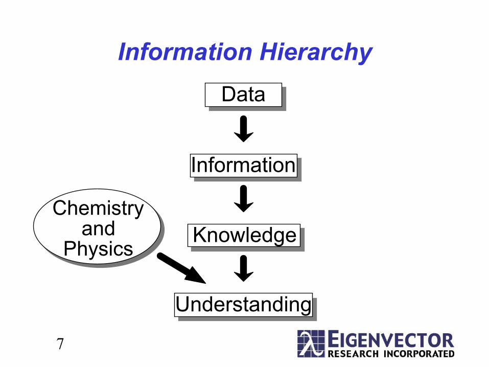
Information HierarchyData

Information

Knowledge

Understanding

Chemistry and

Physics

8

Why Chemometrics?• It’s a multivariate world!

• Need windows into this multivariate world

• There are many things that simply can’t be done if you don’t recognize this, including

• sample classification/pattern recognition• calibrations for complex systems (often spectroscopy)• transfer of calibrations between instruments• fault and upset detection

• Chemometrics focuses on the part of math and statistics applicable to chemical problems

• More expensive to do things with hardware if you can do them with math instead

9

Tools of the Trade

10

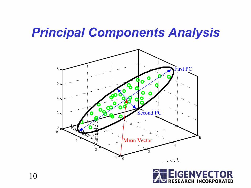
Principal Components Analysis

0

24

6

0

2

4

60

2

4

6

8 First PC

Second PC

i ble 1

Variable 2

Var

iabl

e 3

Mean Vector

11

PCA Math

t1

p1

t2

p2

tk

pk= +

+...+ +

variables

sam

ples X E

The pi are the eigenvectors of the covariance matrix

and the λi are the eigenvalues. Amount of variance captured by tipi proportional to λi.

cov( X ) = X T X m − 1

cov( X ) p i = λ i p i

12

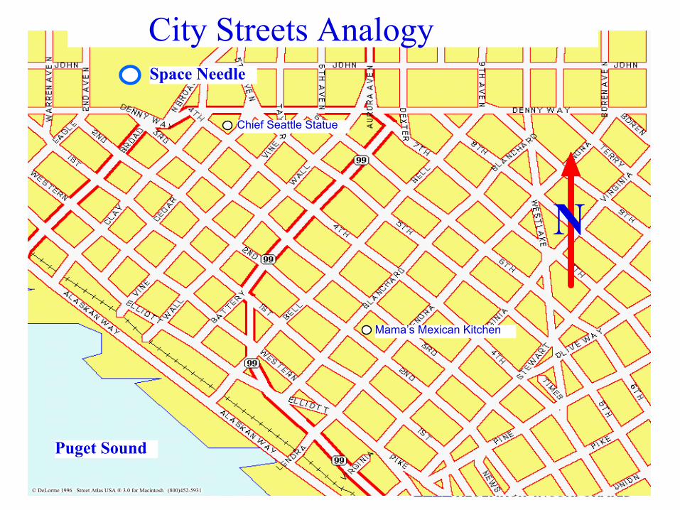
City Streets Analogy

© DeLorme 1996 Street Atlas USA ® 3.0 for Macintosh (800)452-5931 © DeLorme 1996 Street Atlas USA ® 3.0 for Macintosh (800)452-5931 © DeLorme 1996 Street Atlas USA ® 3.0 for Macintosh (800)452-5931 © DeLorme 1996 Street Atlas USA ® 3.0 for Macintosh (800)452-5931 © DeLorme 1996 Street Atlas USA ® 3.0 for Macintosh (800)452-5931 © DeLorme 1996 Street Atlas USA ® 3.0 for Macintosh (800)452-5931 © DeLorme 1996 Street Atlas USA ® 3.0 for Macintosh (800)452-5931 © DeLorme 1996 Street Atlas USA ® 3.0 for Macintosh (800)452-5931 © DeLorme 1996 Street Atlas USA ® 3.0 for Macintosh (800)452-5931 © DeLorme 1996 Street Atlas USA ® 3.0 for Macintosh (800)452-5931 © DeLorme 1996 Street Atlas USA ® 3.0 for Macintosh (800)452-5931 © DeLorme 1996 Street Atlas USA ® 3.0 for Macintosh (800)452-5931 © DeLorme 1996 Street Atlas USA ® 3.0 for Macintosh (800)452-5931

Space Needle

Puget Sound

Mama’s Mexican Kitchen

Chief Seattle Statue

N

City Streets Analogy

13

Properties of PCA

• ti,pi pairs ordered by amount of variance captured• variance = information• ti or scores form an orthogonal set Tk which describe

relationship between samples• pi or loadings form an orthonormal set Pk which

describe relationship between variables

14

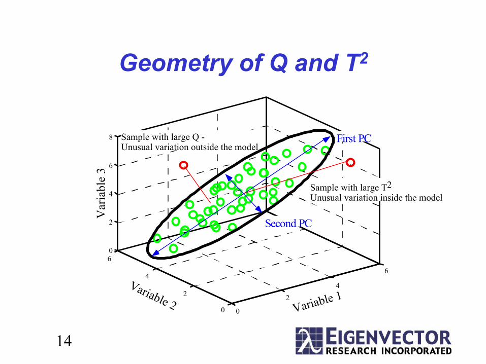
Geometry of Q and T2

0

24

6

0

2

4

60

2

4

6

8 First PC

Second PC

Variable 1Variable 2

Var

iabl

e 3

Sample with large Q -Unusual variation outside the model

Sample with large T2Unusual variation inside the model

15

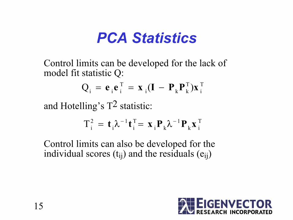
PCA StatisticsControl limits can be developed for the lack of model fit statistic Q:

and Hotelling’s T2 statistic:

Control limits can also be developed for the individual scores (tij) and the residuals (eij)

Q i = e i e Ti = x i ( I − P k P Tk ) x Ti

T 2 i = t i λ − 1 t T

i = x i P k λ − 1 P k x Ti

16

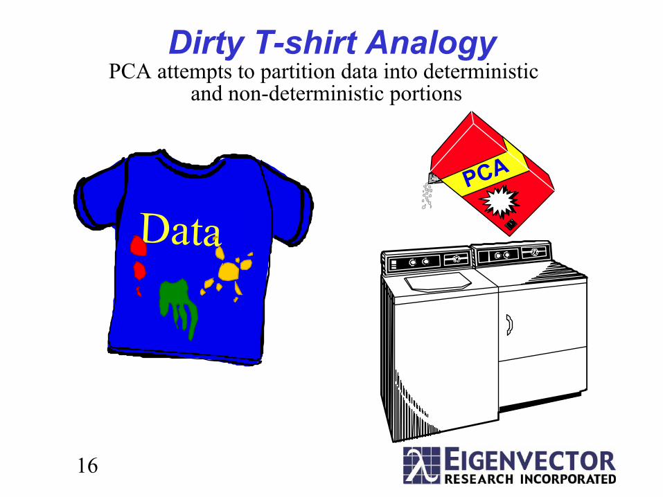
Dirty T-shirt Analogy

DataPCA

PCA attempts to partition data into deterministic and non-deterministic portions

17

Applying a PCA Model to New Data

• A PCA model is a description of a data set, including its mean, amount of variance and its direction, dimensionality, and typical residuals

• New data can be compared with existing PCA models to see if it is “similar”

• Used in Multivariate Statistical Process Control (MSPC)

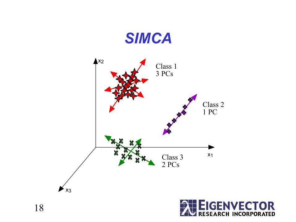
18

SIMCAClass 1 3 PCs

Class 2 1 PC

Class 3 2 PCs

x1

x2

x3

19

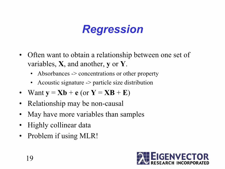
Regression

• Often want to obtain a relationship between one set of variables, X, and another, y or Y.• Absorbances -> concentrations or other property• Acoustic signature -> particle size distribution

• Want y = Xb + e (or Y = XB + E)• Relationship may be non-causal• May have more variables than samples• Highly collinear data• Problem if using MLR!

20

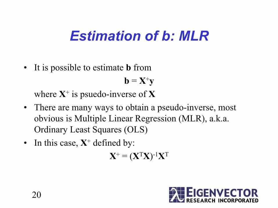
Estimation of b: MLR

• It is possible to estimate b fromb = X+y

where X+ is psuedo-inverse of X• There are many ways to obtain a pseudo-inverse, most

obvious is Multiple Linear Regression (MLR), a.k.a. Ordinary Least Squares (OLS)

• In this case, X+ defined by:X+ = (XTX)-1XT

21

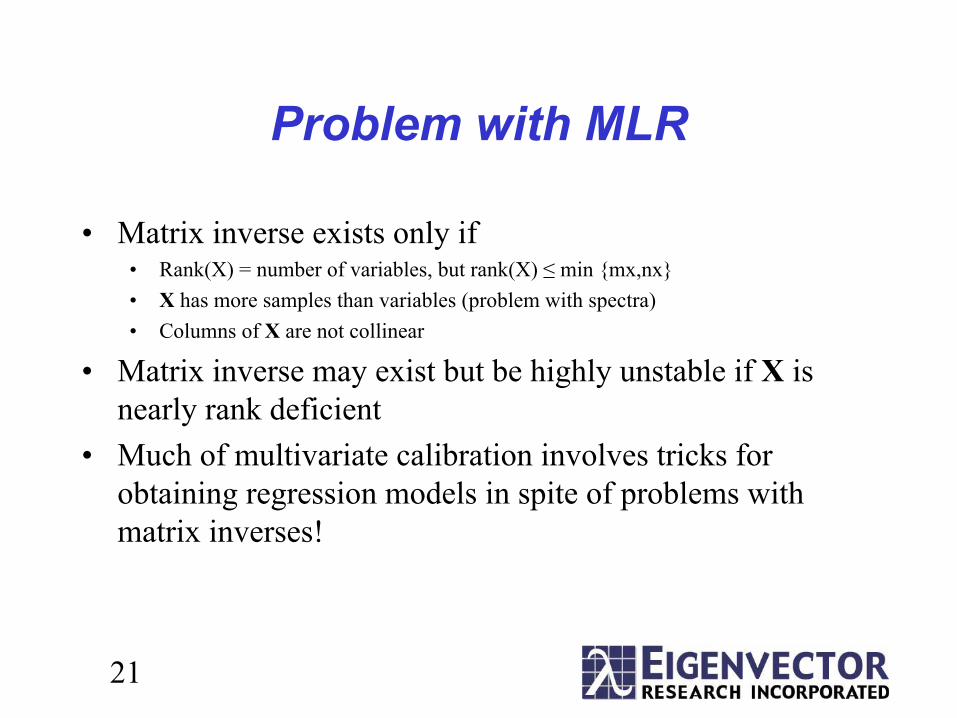
Problem with MLR

• Matrix inverse exists only if • Rank(X) = number of variables, but rank(X) ≤ min {mx,nx}• X has more samples than variables (problem with spectra)• Columns of X are not collinear

• Matrix inverse may exist but be highly unstable if X is nearly rank deficient

• Much of multivariate calibration involves tricks for obtaining regression models in spite of problems with matrix inverses!

22

Getting Around the MLR Problem

• MLR doesn’t work when mx < nx, or when variables are colinear

• Possible solution: eliminate variables, e.g. stepwise regression or other variable selection

• how to choose which variables to keep?• lose multivariate advantage - signal averaging

• Another solution: use PCA to reduce original variables to some smaller number of factors

• retains multivariate advantage• noise reduction aspects of PCA

23

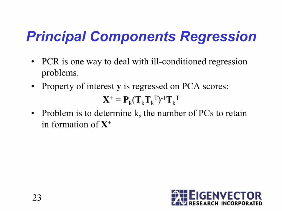
Principal Components Regression• PCR is one way to deal with ill-conditioned regression

problems.• Property of interest y is regressed on PCA scores:

X+ = Pk(TkTkT)-1Tk

T

• Problem is to determine k, the number of PCs to retain in formation of X+

24

Determining the Number of Factors (PCs or LVs)

• A central idea in PCR (and PLS) is that variance is important: use factors that describe lots of variance first

• Question: when do you stop?• Answer: use cross-validation• Build model on part of the data and use remaining data to

test model as a function of number of factors retained

25

Model Cross-validation and Validation

• Cross-validation is a common step in model building• Models should also be validated on totally separate data

sets if possible• Why is this important?• It is very easy to fit data, but making predictions is hard!

26

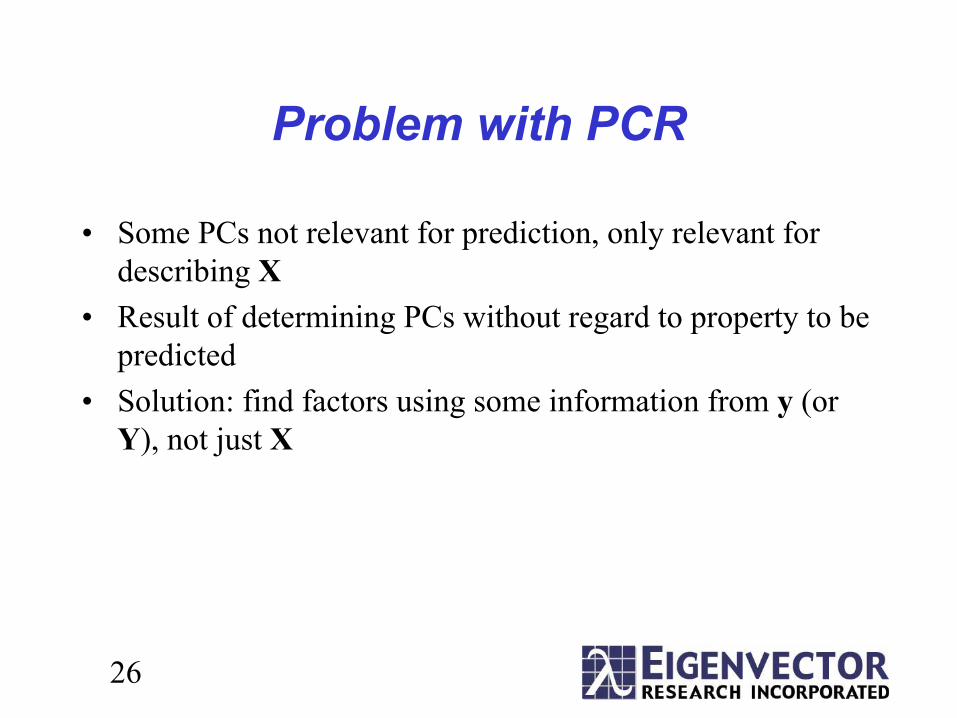
Problem with PCR

• Some PCs not relevant for prediction, only relevant for describing X

• Result of determining PCs without regard to property to be predicted

• Solution: find factors using some information from y (or Y), not just X

27

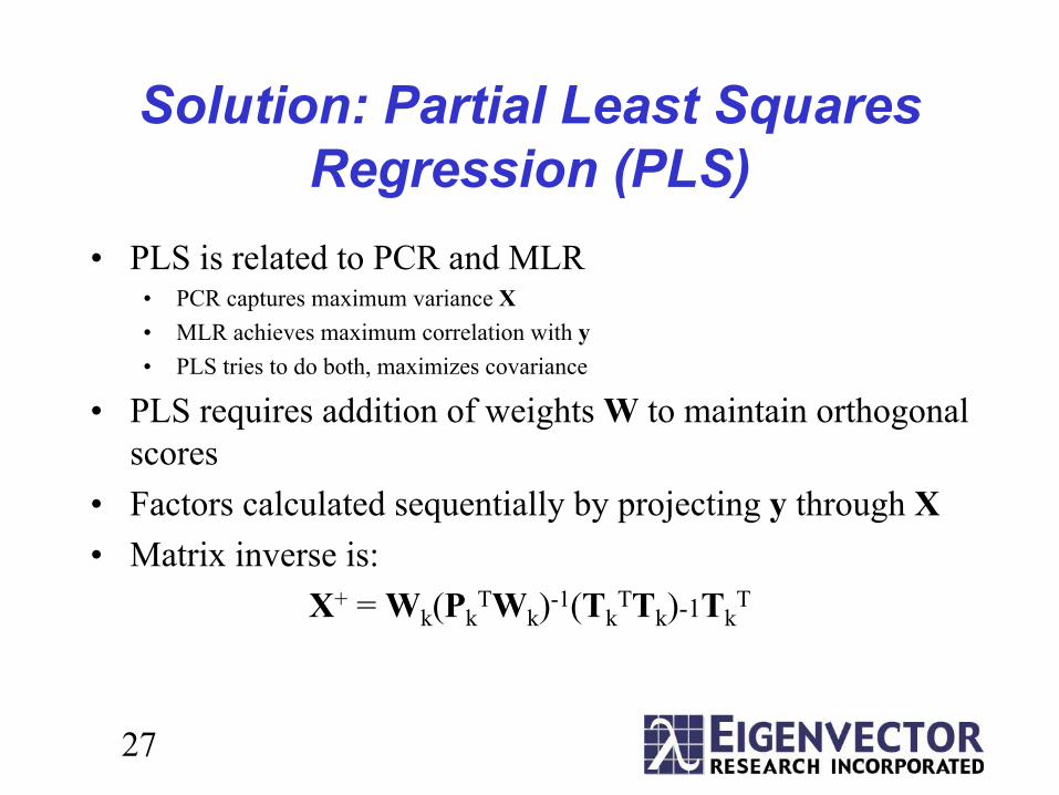
Solution: Partial Least Squares Regression (PLS)

• PLS is related to PCR and MLR• PCR captures maximum variance X• MLR achieves maximum correlation with y• PLS tries to do both, maximizes covariance

• PLS requires addition of weights W to maintain orthogonal scores

• Factors calculated sequentially by projecting y through X• Matrix inverse is:

X+ = Wk(PkTWk)-1(Tk

TTk)-1TkT

28

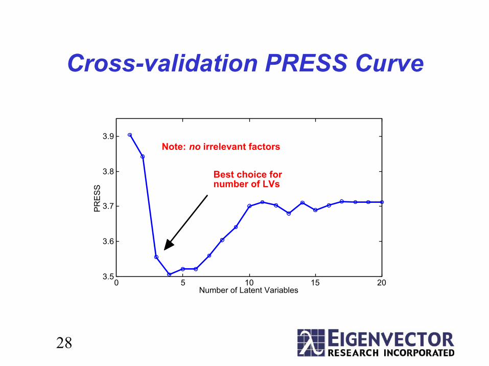
Cross-validation PRESS Curve

0 5 10 15 203.5

3.6

3.7

3.8

3.9

Number of Latent Variables

PRES

S

Best choice for number of LVs

Note: no irrelevant factors

29

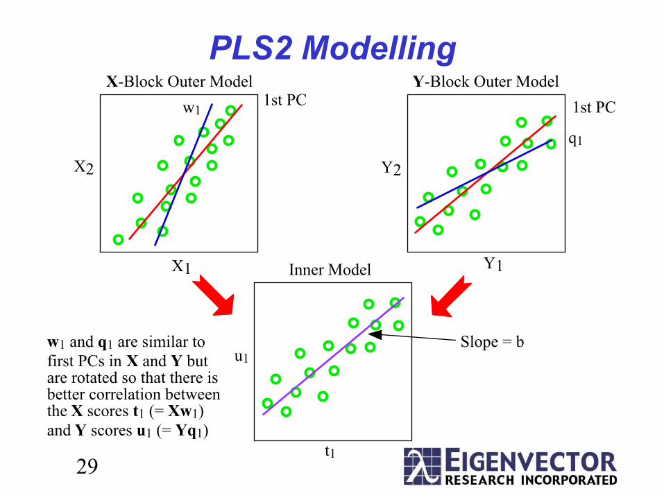
PLS2 Modelling

X1

X2

Y1

Y2

u1

t1

Slope = b

1st PC 1st PCw1

q1

w1 and q1 are similar to first PCs in X and Y but are rotated so that there is better correlation between the X scores t1 (= Xw1) and Y scores u1 (= Yq1)

X-Block Outer Model Y-Block Outer Model

Inner Model

30

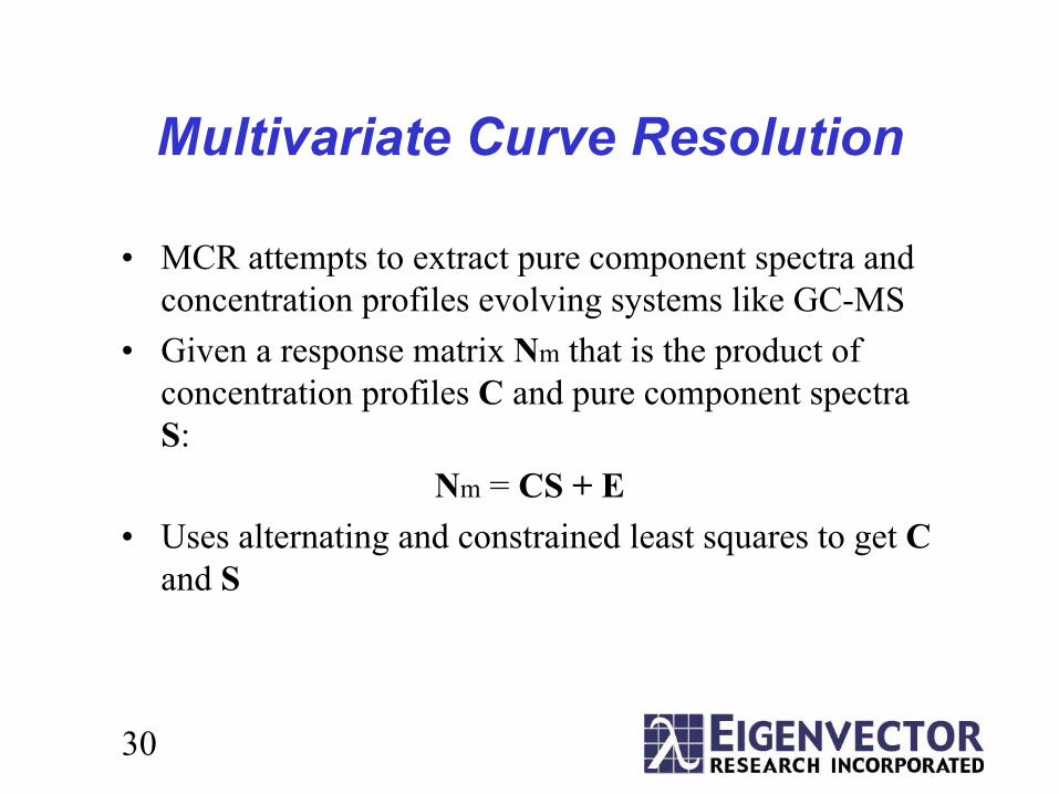
Multivariate Curve Resolution

• MCR attempts to extract pure component spectra and concentration profiles evolving systems like GC-MS

• Given a response matrix Nm that is the product of concentration profiles C and pure component spectra S:

Nm = CS + E• Uses alternating and constrained least squares to get C

and S

31

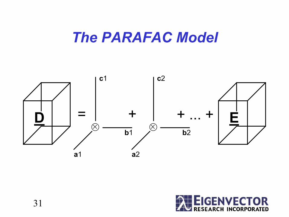
The PARAFAC Model

= + + ... +D

a1

b1

c1

a2

b2

c2

E

32

Opportunities in Process Analytical Technology (PAT)

33

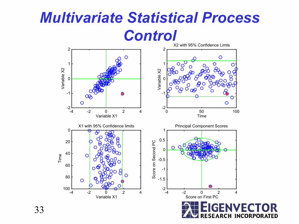
Multivariate Statistical Process Control

Varia

ble

X2

Tim

e

Scor

e on

Sec

ond

PC

Varia

ble

X2

-4 -2 0 2 4-2

-1

0

1

2

Variable X10 50 100

-2

-1

0

1

2

Time

X2 with 95% Confidence Limts

-4 -2 0 2 4

0

20

40

60

80

100

Variable X1

X1 with 95% Confidence limits

-4 -2 0 2 4-2

-1.5

-1

-0.5

0

0.5

1

Score on First PC

Principal Component Scores

34

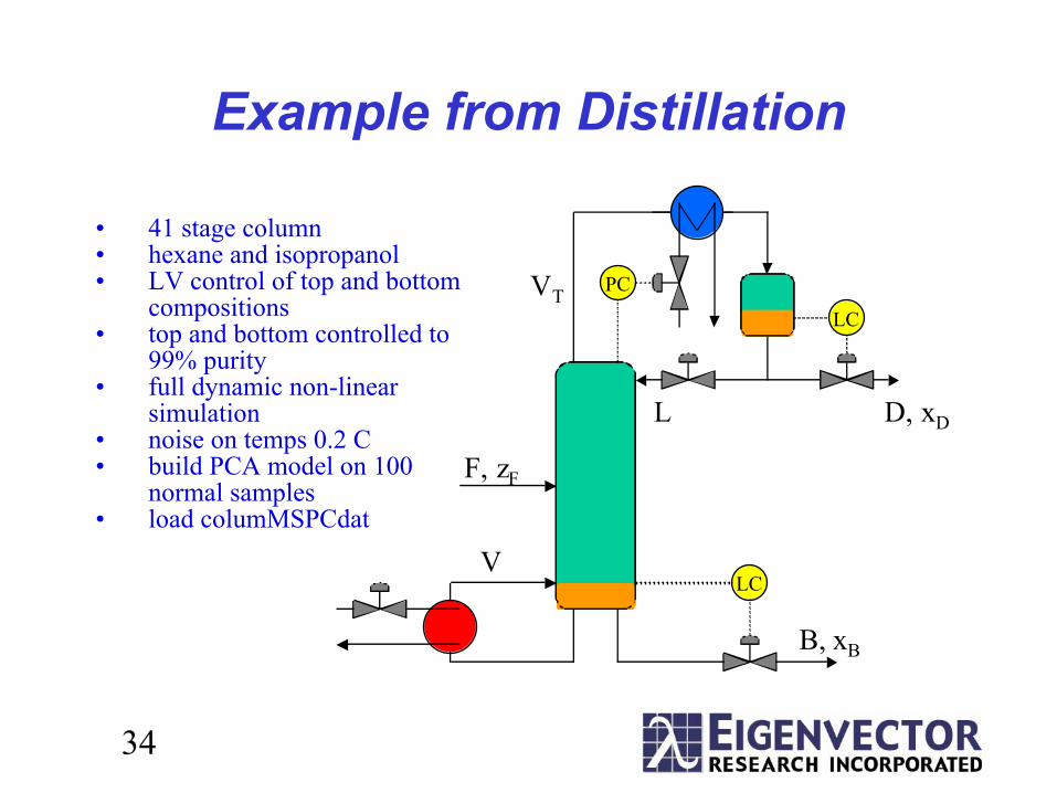
Example from Distillation

LC

LC

PC

F, zF

V

B, xB

D, xDL

VT

• 41 stage column • hexane and isopropanol • LV control of top and bottom

compositions • top and bottom controlled to

99% purity • full dynamic non-linear

simulation • noise on temps 0.2 C • build PCA model on 100

normal samples • load columMSPCdat

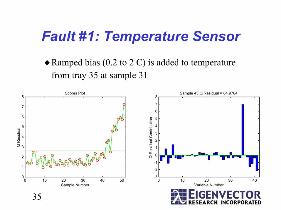
35

Fault #1: Temperature SensorRamped bias (0.2 to 2 C) is added to temperature from tray 35 at sample 31

0 10 20 30 40-3

-2

-1

0

1

2

3

4

5

6

7

8

Variable Number

Q R

esid

ual C

ontri

butio

n

Sample 43 Q Residual = 64.9764

0 10 20 30 40 500

1

2

3

4

5

6

7

8

Sample Number

Q R

esid

ual

Scores Plot

36

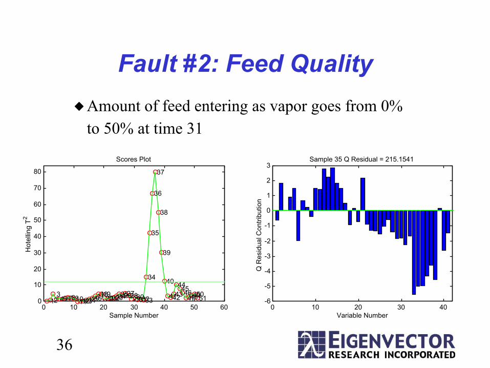
Fault #2: Feed QualityAmount of feed entering as vapor goes from 0% to 50% at time 31

0 10 20 30 40 50 600

10

20

30

40

50

60

70

80

1 2 3 4 5 6 7 8 9 10 11 12 13 14 15 16 17 18 19 20 21 22 23 24 25 26 27 28 29 30 31 32 33

34

35

36

37

38

39

40

41 42 43 44 45 46

47 48 49 50 51

Sample Number

Hot

ellin

g T2

Scores Plot

0 10 20 30 40-6

-5

-4

-3

-2

-1

0

1

2

3

Variable Number

Q R

esid

ual C

ontri

butio

n

Sample 35 Q Residual = 215.1541

37

TOF-SIMS of Time Release Drug Delivery System

• Multilayer drug beads serve as controlled-release delivery system

• TOF-SIMS taken of cross section of bead• Evaluate integrity of layers, distribution of ingredients• Thanks again to Physical Electronics and Anna Belu for

the data!

Reference: A.M. Belu, M.C. Davies, J.M. Newton and N. Patel, “TOF-SIMS Characterization and Imaging of Controlled-Release Drug Delivery Systems, Anal. Chem., 72(22), pps 5625-5638, 2000

38

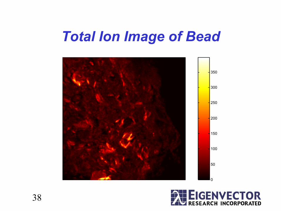
Total Ion Image of Bead

0

50

100

150

200

250

300

350

39

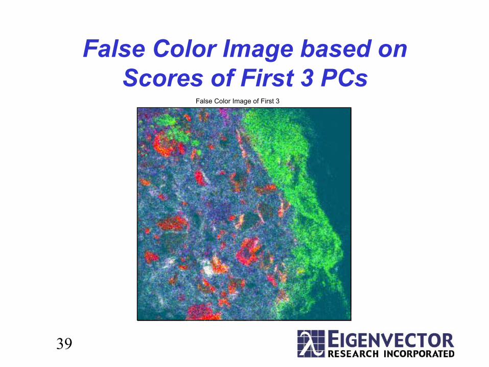
False Color Image based on Scores of First 3 PCs

False Color Image of First 3

40

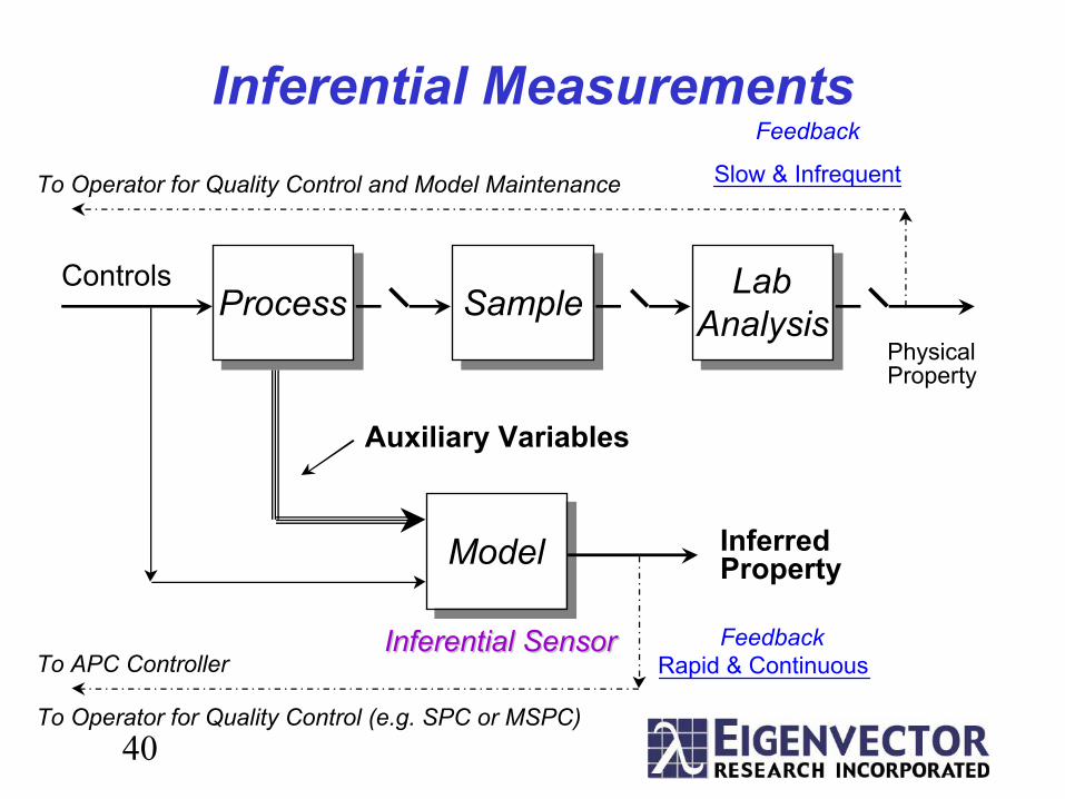
Inferential Measurements

PhysicalProperty

ControlsProcessProcess SampleSample Lab

AnalysisLab

Analysis

ModelModel InferredProperty

Auxiliary Variables

To Operator for Quality Control and Model Maintenance

Inferential SensorInferential SensorTo APC Controller

Feedback

Slow & Infrequent

FeedbackRapid & Continuous

To Operator for Quality Control (e.g. SPC or MSPC)

41

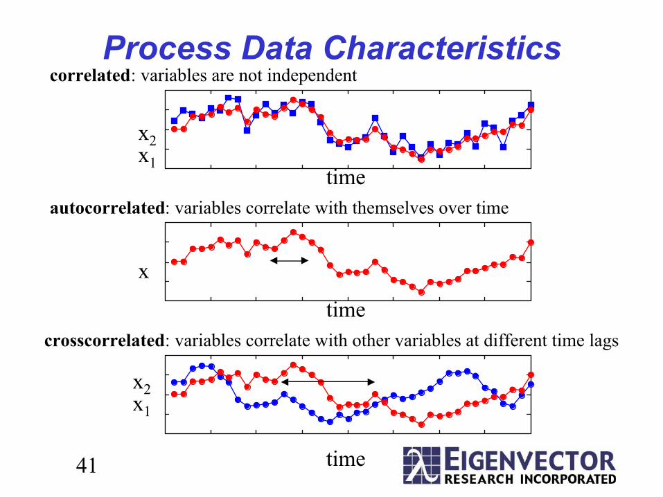
Process Data Characteristics

time

x

time

x1

x2

x1

x2

time

correlated: variables are not independent

autocorrelated: variables correlate with themselves over time

crosscorrelated: variables correlate with other variables at different time lags

42

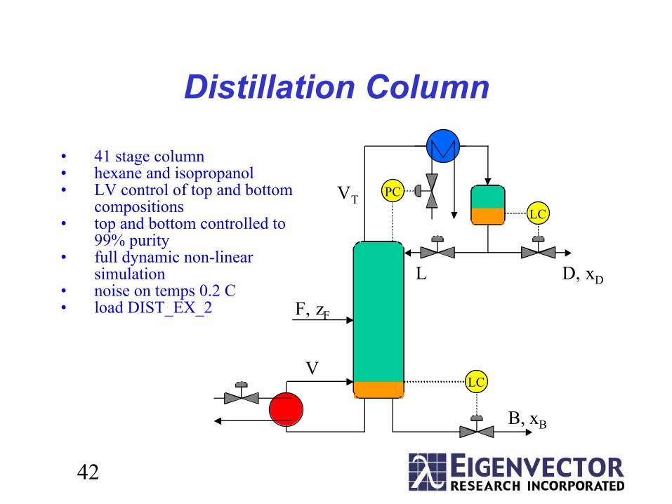
Distillation Column

LC

LC

PC

F, zF

V

B, xB

D, xDL

VT

• 41 stage column • hexane and isopropanol • LV control of top and bottom

compositions • top and bottom controlled to

99% purity • full dynamic non-linear

simulation • noise on temps 0.2 C • load DIST_EX_2

43

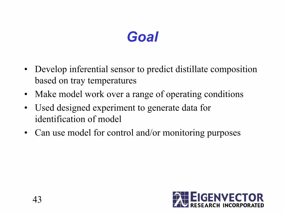
Goal

• Develop inferential sensor to predict distillate composition based on tray temperatures

• Make model work over a range of operating conditions• Used designed experiment to generate data for

identification of model• Can use model for control and/or monitoring purposes

44

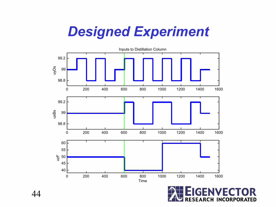
Designed Experiment

0 200 400 600 800 1000 1200 1400 1600

98.8

99

99.2uy

Ds

Inputs to Distillation Column

0 200 400 600 800 1000 1200 1400 1600

98.8

99

99.2

uxBs

0 200 400 600 800 1000 1200 1400 160040

4550

55

60

uzF

Time

45

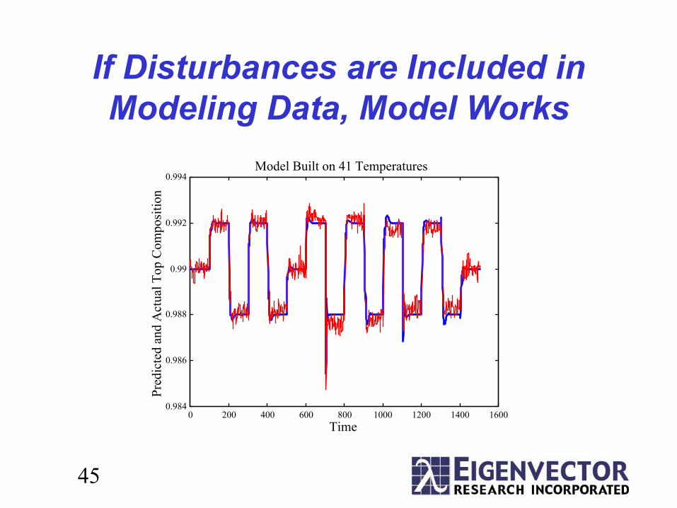
If Disturbances are Included in Modeling Data, Model Works

0 200 400 600 800 1000 1200 1400 16000.984

0.986

0.988

0.99

0.992

0.994

Time

Pred

icte

d an

d A

ctua

l Top

Com

posi

tion

Model Built on 41 Temperatures

46

Batch MSPC

• Multi-way methods can be used to monitor batches

• Build PARAFAC or PARAFAC2 model on normal data, apply to new batches

• Example from semiconductor etch process• Problem: batches often of unequal length!

47

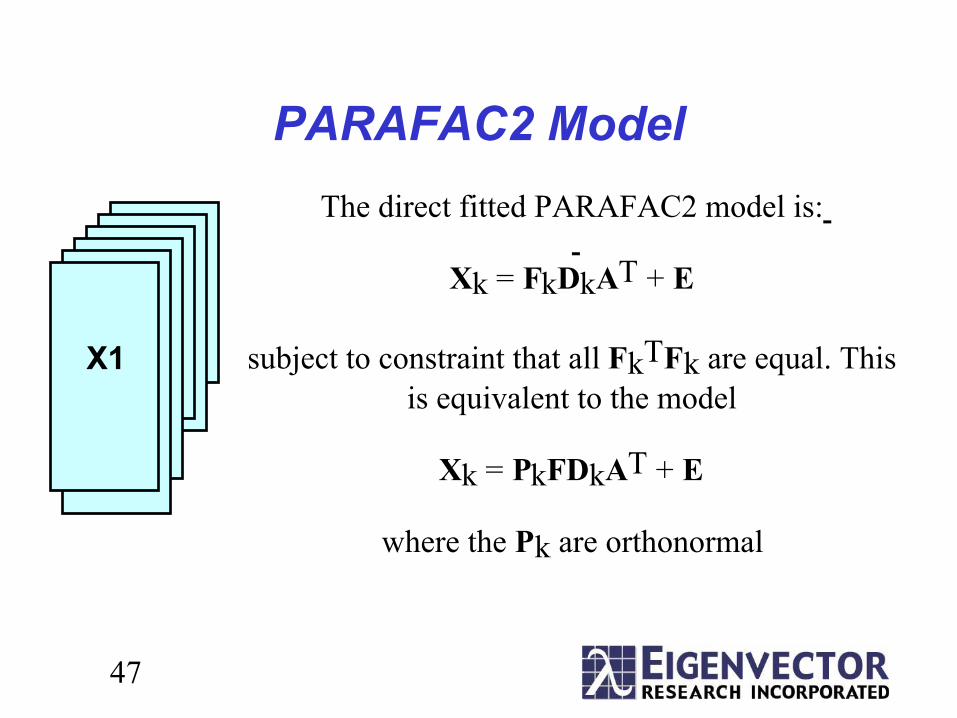
PARAFAC2 Model

X1

The direct fitted PARAFAC2 model is:

Xk = FkDkAT + E

subject to constraint that all FkTFk are equal. Thisis equivalent to the model

Xk = PkFDkAT + E

where the Pk are orthonormal

48

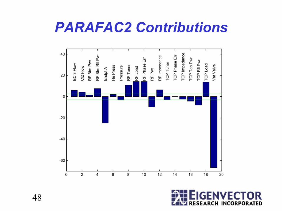
PARAFAC2 Contributions

0 2 4 6 8 10 12 14 16 18 20

-60

-40

-20

0

20

40

BCl3

Flo

w

Cl2

Flo

w

RF

Btm

Pw

r

RF

Btm

Rfl

Pwr

Endp

t A

He

Pres

s

Pres

sure

RF

Tune

r

RF

Load

RF

Phas

e Er

r

RF

Pwr

RF

Impe

danc

e

TCP

Tune

r

TCP

Phas

e Er

r

TCP

Impe

danc

e

TCP

Top

Pwr

TCP

Rfl

Pwr

TCP

Load

Vat V

alve

49

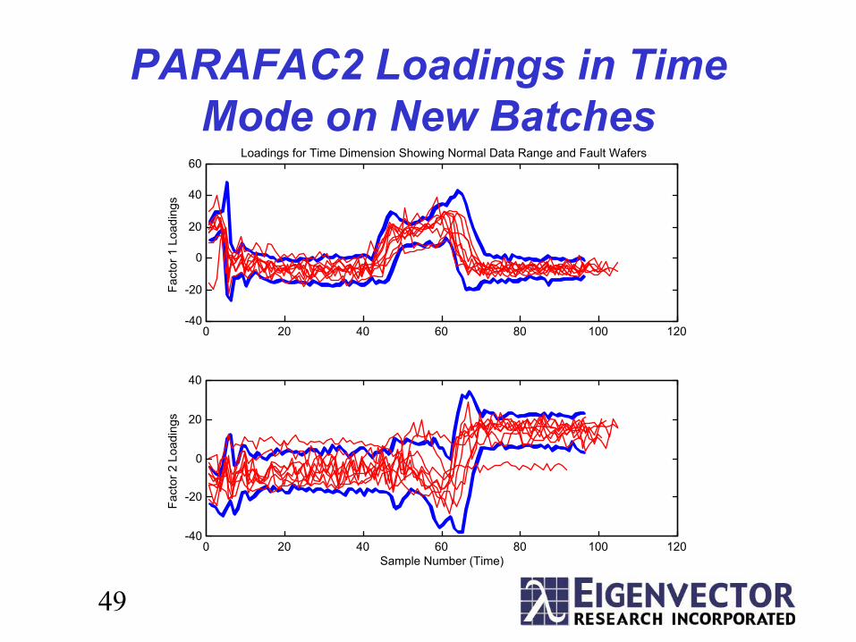
PARAFAC2 Loadings in Time Mode on New Batches

0 20 40 60 80 100 120-40

-20

0

20

40

60Loadings for Time Dimension Showing Normal Data Range and Fault Wafers

Fact

or 1

Loa

ding

s

0 20 40 60 80 100 120-40

-20

0

20

40

Fact

or 2

Loa

ding

s

Sample Number (Time)

50

Summary

• Chemometric tools emphasize • Interpretability• Predictive power

• Many places to use these tools in PAT• MSPC, BSPC• Calibrations, inferentials• Analysis of products

52

Contact InformationEigenvector Research, Inc.830 Wapato Lake RoadManson, WA 98831Phone: (509)687-2022Fax: (509)687-7033Email: bmw@eigenvector.comWeb: eigenvector.com

This document may be downloaded fromhttp://www.eigenvector.com/Docs/Wise_PAT.pdf