Embed Size (px)
Citation preview

Statistical Analysis
with
The General Linear Model1
Jeff Miller and Patricia Haden2
Copyright ( c©) 1988–1990, 1998–2001, 2006.Version: February 16, 2006
1This work is licensed under the Creative Commons Attribution-NonCommercial-NoDerivs 2.5 License. Toview a copy of this license, visit http://creativecommons.org/licenses/by-nc-nd/2.5/ or send a letter to CreativeCommons, 543 Howard Street, 5th Floor, San Francisco, California, 94105, USA. In summary, under thislicense you are free to copy, distribute, and display this work under the following conditions: (1) Attribution:You must attribute this work with the title and authorship as shown on this page. (2) Noncommercial: Youmay not use this work for commercial purposes. (3) No Derivative Works: You may not alter, transform, orbuild upon this work. Furthermore, for any reuse or distribution, you must make clear to others the licenseterms of this work. Any of these conditions can be waived if you get permission from the copyright holder.Your fair use and other rights are in no way affected by the above.
2We thank Profs. Wolfgang Schwarz and Rolf Ulrich for helpful comments and suggestions. Authorcontact address is Prof. Jeff Miller, Department of Psychology, University of Otago, Dunedin, New Zealand,[email protected]. If you use this textbook, we would be delighted to hear about it.

Contents
1 Overview 11.1 The General Linear Model . . . . . . . . . . . . . . . . . . . . . . . . . . . . . . . . . . 1
1.1.1 GLM: ANOVA . . . . . . . . . . . . . . . . . . . . . . . . . . . . . . . . . . . . 11.1.2 GLM: Regression . . . . . . . . . . . . . . . . . . . . . . . . . . . . . . . . . . . 21.1.3 GLM: ANCOVA . . . . . . . . . . . . . . . . . . . . . . . . . . . . . . . . . . . 3
1.2 Learning About the GLM . . . . . . . . . . . . . . . . . . . . . . . . . . . . . . . . . . 41.3 Scientific Research and Alternative Explanations . . . . . . . . . . . . . . . . . . . . . 51.4 The Role of Inferential Statistics in Science . . . . . . . . . . . . . . . . . . . . . . . . 5
I Analysis of Variance 7
2 Introduction to ANOVA 92.1 Terminology for ANOVA Designs . . . . . . . . . . . . . . . . . . . . . . . . . . . . . . 92.2 Summary of ANOVA Terminology . . . . . . . . . . . . . . . . . . . . . . . . . . . . . 112.3 Conclusions from ANOVA . . . . . . . . . . . . . . . . . . . . . . . . . . . . . . . . . . 122.4 Overview of the GLM as used in ANOVA . . . . . . . . . . . . . . . . . . . . . . . . . 122.5 How the GLM Represents the Structure of an Experiment . . . . . . . . . . . . . . . . 12
3 One-Factor, Between-Subject Designs 153.1 The “Variance” in Analysis of Variance . . . . . . . . . . . . . . . . . . . . . . . . . . 153.2 Measuring Between- and Within-Group Variance . . . . . . . . . . . . . . . . . . . . . 173.3 Conceptual Explanations of Estimation Equations . . . . . . . . . . . . . . . . . . . . 203.4 Summary Measures of Variation . . . . . . . . . . . . . . . . . . . . . . . . . . . . . . 213.5 Degrees of Freedom . . . . . . . . . . . . . . . . . . . . . . . . . . . . . . . . . . . . . . 21
3.5.1 Analysis 1 . . . . . . . . . . . . . . . . . . . . . . . . . . . . . . . . . . . . . . . 233.5.2 Analysis 2 . . . . . . . . . . . . . . . . . . . . . . . . . . . . . . . . . . . . . . . 233.5.3 Comparison of Analyses . . . . . . . . . . . . . . . . . . . . . . . . . . . . . . . 233.5.4 Summary of degrees of freedom . . . . . . . . . . . . . . . . . . . . . . . . . . . 24
3.6 Summarizing the Computations in an ANOVA Table . . . . . . . . . . . . . . . . . . . 243.7 Epilogue 1: Why Compare Fobserved to Fcritical? . . . . . . . . . . . . . . . . . . . . . 263.8 Epilogue 2: The Concept of Partitioning . . . . . . . . . . . . . . . . . . . . . . . . . . 283.9 Summary of Computations . . . . . . . . . . . . . . . . . . . . . . . . . . . . . . . . . 293.10 One-Factor Computational Example . . . . . . . . . . . . . . . . . . . . . . . . . . . . 303.11 Review Questions about One-Factor ANOVA . . . . . . . . . . . . . . . . . . . . . . . 303.12 Computational Exercises . . . . . . . . . . . . . . . . . . . . . . . . . . . . . . . . . . . 313.13 Answers to Exercises . . . . . . . . . . . . . . . . . . . . . . . . . . . . . . . . . . . . . 31
4 Two-Factor, Between-Subject Designs 354.1 The Information in Two-Factor Experiments . . . . . . . . . . . . . . . . . . . . . . . 354.2 The Concept of a Two-Factor Interaction . . . . . . . . . . . . . . . . . . . . . . . . . 384.3 The GLM for Two-Factor Between-Subjects Designs . . . . . . . . . . . . . . . . . . . 424.4 Computations for Two-Factor Between-Subjects Designs . . . . . . . . . . . . . . . . . 424.5 Drawing Conclusions About Two-Factor Designs . . . . . . . . . . . . . . . . . . . . . 484.6 Summary of Computations . . . . . . . . . . . . . . . . . . . . . . . . . . . . . . . . . 494.7 Relationships Between One- and Two-Factor ANOVA . . . . . . . . . . . . . . . . . . 504.8 Review Questions about Two-Factor ANOVA . . . . . . . . . . . . . . . . . . . . . . . 524.9 Exercises on Two-Way Between-Ss ANOVA . . . . . . . . . . . . . . . . . . . . . . . . 52
i

ii CONTENTS
4.10 Answers to Exercises . . . . . . . . . . . . . . . . . . . . . . . . . . . . . . . . . . . . . 53
5 Three-Factor, Between-Subject Designs 575.1 A More General Conceptual Overview of ANOVA . . . . . . . . . . . . . . . . . . . . 575.2 ANOVA Computations for Three-Factor Between-Ss Designs . . . . . . . . . . . . . . 58
5.2.1 Model . . . . . . . . . . . . . . . . . . . . . . . . . . . . . . . . . . . . . . . . . 585.2.2 Estimation . . . . . . . . . . . . . . . . . . . . . . . . . . . . . . . . . . . . . . 595.2.3 Decomposition Matrix and SS’s . . . . . . . . . . . . . . . . . . . . . . . . . . 605.2.4 Degrees of Freedom . . . . . . . . . . . . . . . . . . . . . . . . . . . . . . . . . 615.2.5 ANOVA Table . . . . . . . . . . . . . . . . . . . . . . . . . . . . . . . . . . . . 61
5.3 Interpreting Three-Factor ANOVAs . . . . . . . . . . . . . . . . . . . . . . . . . . . . . 625.3.1 Strategy 1: How does a two-way interaction change? . . . . . . . . . . . . . . . 635.3.2 Strategy 2: How does a main effect change? . . . . . . . . . . . . . . . . . . . . 645.3.3 Summary . . . . . . . . . . . . . . . . . . . . . . . . . . . . . . . . . . . . . . . 65
5.4 Exercises: Three-Factor, Between-Ss ANOVA . . . . . . . . . . . . . . . . . . . . . . . 655.5 Answers to Exercises . . . . . . . . . . . . . . . . . . . . . . . . . . . . . . . . . . . . . 66
6 Generalization of Between-Subject Designs 716.1 Constructing the model . . . . . . . . . . . . . . . . . . . . . . . . . . . . . . . . . . . 71
6.1.1 The Order of the Terms in the Model . . . . . . . . . . . . . . . . . . . . . . . 726.2 Subscripts . . . . . . . . . . . . . . . . . . . . . . . . . . . . . . . . . . . . . . . . . . . 736.3 Estimation . . . . . . . . . . . . . . . . . . . . . . . . . . . . . . . . . . . . . . . . . . 736.4 Computing SS’s and df’s . . . . . . . . . . . . . . . . . . . . . . . . . . . . . . . . . . 746.5 Computing MS’s and F’s . . . . . . . . . . . . . . . . . . . . . . . . . . . . . . . . . . 756.6 Interpreting significant F’s . . . . . . . . . . . . . . . . . . . . . . . . . . . . . . . . . . 756.7 Exercise: Four-Factor Design . . . . . . . . . . . . . . . . . . . . . . . . . . . . . . . . 75
7 Within-Subjects Designs 797.1 Within- vs. Between-Subject Designs . . . . . . . . . . . . . . . . . . . . . . . . . . . . 797.2 Models for Within-Ss Designs . . . . . . . . . . . . . . . . . . . . . . . . . . . . . . . . 817.3 Estimation and Decomposition . . . . . . . . . . . . . . . . . . . . . . . . . . . . . . . 867.4 “Random-Effects” vs. “Fixed-Effects” Factors . . . . . . . . . . . . . . . . . . . . . . . 887.5 Choice of Error Term & Computation of Fobserved . . . . . . . . . . . . . . . . . . . . 89
7.5.1 Error as a “Yardstick” . . . . . . . . . . . . . . . . . . . . . . . . . . . . . . . . 897.5.2 Error Term for µ . . . . . . . . . . . . . . . . . . . . . . . . . . . . . . . . . . . 897.5.3 Error Term for a Main Effect . . . . . . . . . . . . . . . . . . . . . . . . . . . . 907.5.4 Error Terms for Interactions . . . . . . . . . . . . . . . . . . . . . . . . . . . . . 917.5.5 Error Term Summary . . . . . . . . . . . . . . . . . . . . . . . . . . . . . . . . 917.5.6 Comparison with Between-Subjects Designs . . . . . . . . . . . . . . . . . . . . 91
7.6 Interpretation of F’s . . . . . . . . . . . . . . . . . . . . . . . . . . . . . . . . . . . . . 927.7 Computational Examples . . . . . . . . . . . . . . . . . . . . . . . . . . . . . . . . . . 927.8 Exercises . . . . . . . . . . . . . . . . . . . . . . . . . . . . . . . . . . . . . . . . . . . 997.9 Answers to Exercises . . . . . . . . . . . . . . . . . . . . . . . . . . . . . . . . . . . . . 101
8 Mixed Designs—The General Case 1038.1 Linear Model . . . . . . . . . . . . . . . . . . . . . . . . . . . . . . . . . . . . . . . . . 1038.2 Estimation Equations and SS’s . . . . . . . . . . . . . . . . . . . . . . . . . . . . . . . 1068.3 Degrees of Freedom . . . . . . . . . . . . . . . . . . . . . . . . . . . . . . . . . . . . . . 1078.4 Error Terms . . . . . . . . . . . . . . . . . . . . . . . . . . . . . . . . . . . . . . . . . . 1078.5 Order Effects . . . . . . . . . . . . . . . . . . . . . . . . . . . . . . . . . . . . . . . . . 109
9 Shortcut for Computing Sums of Squares 1139.1 One-Factor Between-Ss Example . . . . . . . . . . . . . . . . . . . . . . . . . . . . . . 1139.2 Three-Factor Between-Ss Example . . . . . . . . . . . . . . . . . . . . . . . . . . . . . 1149.3 Two-Factor Within-Ss Example . . . . . . . . . . . . . . . . . . . . . . . . . . . . . . . 117

CONTENTS iii
II Regression 119
10 Introduction to Correlation and Regression 12110.1 A Conceptual Example . . . . . . . . . . . . . . . . . . . . . . . . . . . . . . . . . . . . 12110.2 Overview . . . . . . . . . . . . . . . . . . . . . . . . . . . . . . . . . . . . . . . . . . . 125
11 Simple Correlation 12711.1 The Scattergram . . . . . . . . . . . . . . . . . . . . . . . . . . . . . . . . . . . . . . . 12811.2 Types of Bivariate Relationships . . . . . . . . . . . . . . . . . . . . . . . . . . . . . . 12811.3 The Correlation Coefficient . . . . . . . . . . . . . . . . . . . . . . . . . . . . . . . . . 13011.4 Testing the Null Hypothesis of No Correlation . . . . . . . . . . . . . . . . . . . . . . . 13211.5 Conclusions from Significant and Nonsignificant Correlations . . . . . . . . . . . . . . 133
11.5.1 Significant Correlations . . . . . . . . . . . . . . . . . . . . . . . . . . . . . . . 13311.5.2 Nonsignificant Correlations . . . . . . . . . . . . . . . . . . . . . . . . . . . . . 134
11.6 The Correlation Matrix . . . . . . . . . . . . . . . . . . . . . . . . . . . . . . . . . . . 135
12 Simple Regression 13712.1 The Simple Regression Model . . . . . . . . . . . . . . . . . . . . . . . . . . . . . . . . 13712.2 Fitting the Model to the Data . . . . . . . . . . . . . . . . . . . . . . . . . . . . . . . . 13912.3 ANOVA Table for Simple Regression . . . . . . . . . . . . . . . . . . . . . . . . . . . . 14012.4 Critical F ’s and Conclusions . . . . . . . . . . . . . . . . . . . . . . . . . . . . . . . . . 143
12.4.1 Significant Slope . . . . . . . . . . . . . . . . . . . . . . . . . . . . . . . . . . . 14312.4.2 Nonsignificant Slope . . . . . . . . . . . . . . . . . . . . . . . . . . . . . . . . . 14312.4.3 Intercept . . . . . . . . . . . . . . . . . . . . . . . . . . . . . . . . . . . . . . . 144
12.5 Relation of Simple Regression to Simple Correlation . . . . . . . . . . . . . . . . . . . 144
13 Traps and Pitfalls in Regression Analysis 14713.1 Effects of Pooling Distinct Groups . . . . . . . . . . . . . . . . . . . . . . . . . . . . . 147
13.1.1 Implications for Interpretation . . . . . . . . . . . . . . . . . . . . . . . . . . . 14713.1.2 Precautions . . . . . . . . . . . . . . . . . . . . . . . . . . . . . . . . . . . . . . 148
13.2 Range Restriction Reduces Correlations . . . . . . . . . . . . . . . . . . . . . . . . . . 14913.2.1 Implications for Interpretation . . . . . . . . . . . . . . . . . . . . . . . . . . . 15013.2.2 Precautions . . . . . . . . . . . . . . . . . . . . . . . . . . . . . . . . . . . . . . 150
13.3 Effects of Measurement Error . . . . . . . . . . . . . . . . . . . . . . . . . . . . . . . . 15013.3.1 Implications for Interpretation . . . . . . . . . . . . . . . . . . . . . . . . . . . 15113.3.2 Precautions . . . . . . . . . . . . . . . . . . . . . . . . . . . . . . . . . . . . . . 152
13.4 Applying the Model to New Cases . . . . . . . . . . . . . . . . . . . . . . . . . . . . . 15213.4.1 Implications for Interpretation . . . . . . . . . . . . . . . . . . . . . . . . . . . 15313.4.2 Precautions . . . . . . . . . . . . . . . . . . . . . . . . . . . . . . . . . . . . . . 153
13.5 Regression Towards the Mean . . . . . . . . . . . . . . . . . . . . . . . . . . . . . . . . 15313.5.1 Implications for Interpretation . . . . . . . . . . . . . . . . . . . . . . . . . . . 15613.5.2 Precautions . . . . . . . . . . . . . . . . . . . . . . . . . . . . . . . . . . . . . . 158
14 Multiple Regression 15914.1 Introduction . . . . . . . . . . . . . . . . . . . . . . . . . . . . . . . . . . . . . . . . . . 15914.2 The Model for Multiple Regression . . . . . . . . . . . . . . . . . . . . . . . . . . . . . 15914.3 A Limitation: One F per Model . . . . . . . . . . . . . . . . . . . . . . . . . . . . . . 16014.4 Computations . . . . . . . . . . . . . . . . . . . . . . . . . . . . . . . . . . . . . . . . . 161
14.4.1 Estimation of a and the b’s . . . . . . . . . . . . . . . . . . . . . . . . . . . . . 16114.4.2 Predicted Y Values . . . . . . . . . . . . . . . . . . . . . . . . . . . . . . . . . . 16114.4.3 Error Estimates . . . . . . . . . . . . . . . . . . . . . . . . . . . . . . . . . . . . 16214.4.4 Sums of Squares . . . . . . . . . . . . . . . . . . . . . . . . . . . . . . . . . . . 16214.4.5 Degrees of Freedom . . . . . . . . . . . . . . . . . . . . . . . . . . . . . . . . . 16314.4.6 Summary ANOVA Table . . . . . . . . . . . . . . . . . . . . . . . . . . . . . . 163
14.5 Interpretation & Conclusions . . . . . . . . . . . . . . . . . . . . . . . . . . . . . . . . 16314.5.1 The Null Hypothesis . . . . . . . . . . . . . . . . . . . . . . . . . . . . . . . . . 16314.5.2 What to Conclude When H0 is Rejected . . . . . . . . . . . . . . . . . . . . . . 16414.5.3 What to Conclude When H0 is Not Rejected . . . . . . . . . . . . . . . . . . . 164
14.6 Discussion . . . . . . . . . . . . . . . . . . . . . . . . . . . . . . . . . . . . . . . . . . . 164

iv CONTENTS
15 Extra Sum of Squares Comparisons 16715.1 Overview and Example . . . . . . . . . . . . . . . . . . . . . . . . . . . . . . . . . . . . 16715.2 Computations . . . . . . . . . . . . . . . . . . . . . . . . . . . . . . . . . . . . . . . . . 16915.3 Conclusions & Interpretation . . . . . . . . . . . . . . . . . . . . . . . . . . . . . . . . 170
15.3.1 The Null Hypothesis . . . . . . . . . . . . . . . . . . . . . . . . . . . . . . . . . 17015.3.2 Interpretation of a Significant Extra F . . . . . . . . . . . . . . . . . . . . . . . 17115.3.3 Interpretation of a Nonsignificant Extra F . . . . . . . . . . . . . . . . . . . . . 172
15.4 Discussion . . . . . . . . . . . . . . . . . . . . . . . . . . . . . . . . . . . . . . . . . . . 17215.4.1 Measurement by subtraction. . . . . . . . . . . . . . . . . . . . . . . . . . . . . 17215.4.2 Controlling for potential confounding variables. . . . . . . . . . . . . . . . . . . 17215.4.3 When would you use more than one “extra” predictor? . . . . . . . . . . . . . 173
15.5 Fadd and Fdrop . . . . . . . . . . . . . . . . . . . . . . . . . . . . . . . . . . . . . . . . 174
16 Relationships Among Predictors 17716.1 Context Effects . . . . . . . . . . . . . . . . . . . . . . . . . . . . . . . . . . . . . . . . 17716.2 Redundancy . . . . . . . . . . . . . . . . . . . . . . . . . . . . . . . . . . . . . . . . . . 178
16.2.1 SS Thinning . . . . . . . . . . . . . . . . . . . . . . . . . . . . . . . . . . . . . 18116.3 Reduction of Error in Y . . . . . . . . . . . . . . . . . . . . . . . . . . . . . . . . . . . 18216.4 Suppression of Error in X . . . . . . . . . . . . . . . . . . . . . . . . . . . . . . . . . . 18316.5 Venn Diagrams—Optional Section . . . . . . . . . . . . . . . . . . . . . . . . . . . . . 18516.6 Mixing Positive and Negative Correlations . . . . . . . . . . . . . . . . . . . . . . . . . 186
16.6.1 Redundancy . . . . . . . . . . . . . . . . . . . . . . . . . . . . . . . . . . . . . . 18616.6.2 Reduction of Error in Y . . . . . . . . . . . . . . . . . . . . . . . . . . . . . . . 18716.6.3 Suppression of Error in X . . . . . . . . . . . . . . . . . . . . . . . . . . . . . . 187
17 Finding the Best Model 18917.1 What is the Best Model? . . . . . . . . . . . . . . . . . . . . . . . . . . . . . . . . . . 18917.2 All Possible Models Procedure . . . . . . . . . . . . . . . . . . . . . . . . . . . . . . . 190
17.2.1 Illustration with data of Table 17.1. . . . . . . . . . . . . . . . . . . . . . . . . 19017.2.2 Discussion . . . . . . . . . . . . . . . . . . . . . . . . . . . . . . . . . . . . . . . 191
17.3 Forward Selection Procedure . . . . . . . . . . . . . . . . . . . . . . . . . . . . . . . . 19217.3.1 Illustration with data of Table 17.1. . . . . . . . . . . . . . . . . . . . . . . . . 19217.3.2 Discussion . . . . . . . . . . . . . . . . . . . . . . . . . . . . . . . . . . . . . . . 195
17.4 Backward Elimination Procedure . . . . . . . . . . . . . . . . . . . . . . . . . . . . . . 19617.4.1 Illustration with data of Table 17.1. . . . . . . . . . . . . . . . . . . . . . . . . 19617.4.2 Discussion . . . . . . . . . . . . . . . . . . . . . . . . . . . . . . . . . . . . . . . 197
17.5 Stepwise Procedure . . . . . . . . . . . . . . . . . . . . . . . . . . . . . . . . . . . . . . 19817.5.1 Illustration with data of Table 17.1. . . . . . . . . . . . . . . . . . . . . . . . . 19817.5.2 Discussion . . . . . . . . . . . . . . . . . . . . . . . . . . . . . . . . . . . . . . . 203
17.6 How Much Can You Trust the “Best Model” . . . . . . . . . . . . . . . . . . . . . . . 20417.6.1 Finding the Best Model for the Sample . . . . . . . . . . . . . . . . . . . . . . 20417.6.2 Finding the Best Model for the Population . . . . . . . . . . . . . . . . . . . . 204
III Analysis of Covariance 209
18 Dummy Variable Regression 21118.1 Overview . . . . . . . . . . . . . . . . . . . . . . . . . . . . . . . . . . . . . . . . . . . 21118.2 The General Linear Model for DVR and ANCOVA . . . . . . . . . . . . . . . . . . . . 21118.3 Computations For DVR . . . . . . . . . . . . . . . . . . . . . . . . . . . . . . . . . . . 21218.4 Effects Coding . . . . . . . . . . . . . . . . . . . . . . . . . . . . . . . . . . . . . . . . 21218.5 Example 1 . . . . . . . . . . . . . . . . . . . . . . . . . . . . . . . . . . . . . . . . . . . 21318.6 Example 2 . . . . . . . . . . . . . . . . . . . . . . . . . . . . . . . . . . . . . . . . . . . 21418.7 Example 3 . . . . . . . . . . . . . . . . . . . . . . . . . . . . . . . . . . . . . . . . . . . 21418.8 Using Dummy Variables To Perform ANOVA . . . . . . . . . . . . . . . . . . . . . . . 217
18.8.1 Computations for Example 1 . . . . . . . . . . . . . . . . . . . . . . . . . . . . 21818.8.2 Computations for Example 2 . . . . . . . . . . . . . . . . . . . . . . . . . . . . 21818.8.3 Computations for Example 3 . . . . . . . . . . . . . . . . . . . . . . . . . . . . 219
18.9 The Relationship of ANOVA to DVR . . . . . . . . . . . . . . . . . . . . . . . . . . . . 22118.9.1 Models and Parameters . . . . . . . . . . . . . . . . . . . . . . . . . . . . . . . 221

CONTENTS v
18.9.2 DVR Computations by Computer . . . . . . . . . . . . . . . . . . . . . . . . . 22318.9.3 ANOVA With Unequal Cell Sizes (Weighted Means Solution) . . . . . . . . . . 22318.9.4 Context effects in ANOVA . . . . . . . . . . . . . . . . . . . . . . . . . . . . . 223
18.10Interactions Of ANOVA Factors and Covariates . . . . . . . . . . . . . . . . . . . . . . 22418.11Principles of Data Analysis Using DVR . . . . . . . . . . . . . . . . . . . . . . . . . . 22518.12Example 4: One Factor and One Covariate . . . . . . . . . . . . . . . . . . . . . . . . 22518.13Changing the Y-Intercept . . . . . . . . . . . . . . . . . . . . . . . . . . . . . . . . . . 22718.14Example: A Factorial Analysis of Slopes . . . . . . . . . . . . . . . . . . . . . . . . . . 228
18.14.1 Interpretations of Intercept Effects . . . . . . . . . . . . . . . . . . . . . . . . . 23118.14.2 Interpretation of Slope Effects . . . . . . . . . . . . . . . . . . . . . . . . . . . . 231
18.15Multiple Covariates Example . . . . . . . . . . . . . . . . . . . . . . . . . . . . . . . . 232
19 Analysis of Covariance 23519.1 Goals of ANCOVA . . . . . . . . . . . . . . . . . . . . . . . . . . . . . . . . . . . . . . 23519.2 How ANCOVA Reduces Error . . . . . . . . . . . . . . . . . . . . . . . . . . . . . . . . 23519.3 ANCOVA Computational Procedure . . . . . . . . . . . . . . . . . . . . . . . . . . . . 23819.4 ANCOVA Assumptions . . . . . . . . . . . . . . . . . . . . . . . . . . . . . . . . . . . 240
A The AnoGen Program 245A.1 Introduction . . . . . . . . . . . . . . . . . . . . . . . . . . . . . . . . . . . . . . . . . . 245A.2 Step-by-Step Instructions: Student Mode . . . . . . . . . . . . . . . . . . . . . . . . . 245A.3 Explanation of Problem Display . . . . . . . . . . . . . . . . . . . . . . . . . . . . . . . 246A.4 Explanation of Solution Display . . . . . . . . . . . . . . . . . . . . . . . . . . . . . . . 246
A.4.1 Design . . . . . . . . . . . . . . . . . . . . . . . . . . . . . . . . . . . . . . . . . 247A.4.2 Cell Means . . . . . . . . . . . . . . . . . . . . . . . . . . . . . . . . . . . . . . 247A.4.3 Model . . . . . . . . . . . . . . . . . . . . . . . . . . . . . . . . . . . . . . . . . 247A.4.4 Estimation Equations . . . . . . . . . . . . . . . . . . . . . . . . . . . . . . . . 248A.4.5 Decomposition Matrix . . . . . . . . . . . . . . . . . . . . . . . . . . . . . . . . 248A.4.6 ANOVA Table . . . . . . . . . . . . . . . . . . . . . . . . . . . . . . . . . . . . 248
B Statistical Tables 249B.1 F -Critical Values . . . . . . . . . . . . . . . . . . . . . . . . . . . . . . . . . . . . . . . 250B.2 Critical Values of Correlation Coefficient (Pearson r) . . . . . . . . . . . . . . . . . . . 257
Bibliography 259

vi CONTENTS

List of Figures
1.1 Average blood cholesterol levels (shown on the vertical axis) of males and femaleswithin each of five ethnic groups representing North America (NA), South America(SA), Europe (Eur), Asia, and the Pacific islands (Pac). . . . . . . . . . . . . . . . . . 2
1.2 Scattergram showing the relationship between age and blood cholesterol level for asample of 23 individuals, each represented by one square on the graph. . . . . . . . . . 3
1.3 Scattergram showing the relationship between age and blood cholesterol level separatelyfor males and females. . . . . . . . . . . . . . . . . . . . . . . . . . . . . . . . . . . . . 3
3.1 Plot of Spelling Data Values . . . . . . . . . . . . . . . . . . . . . . . . . . . . . . . . . 163.2 Example F Distributions. Each panel shows the theoretical distribution of Fobserved
for the indicated number of degrees of freedom in the numerator and denominator. Alldistributions were computed under the assumption that the null hypothesis is true. Foreach distribution, the critical value is indicated by the vertical line. This is the valuethat cuts off the upper 5% of the distribution—i.e., that Fobserved will exceed only 5%of the time. . . . . . . . . . . . . . . . . . . . . . . . . . . . . . . . . . . . . . . . . . . 27
4.1 Factorial plots showing three different sets of possible results for an experiment testingamount of learning as a function of gender of student and gender of teacher. . . . . . . 36
4.2 Factorial plots of hypothetical results showing liking for a sandwich as a function ofpresence/absence of peanut butter and presence/absence of bologna. . . . . . . . . . . 39
4.3 Factorial plots of hypothetical results showing sharp-shooting accuracy as a function ofright eye open vs. closed and left eye open vs. closed. . . . . . . . . . . . . . . . . . . . 39
5.1 Sentence as a function of genders of A) defendant and juror; B) defendant and prosecutor;and C) prosecutor and juror. . . . . . . . . . . . . . . . . . . . . . . . . . . . . . . . . 63
5.2 Sentence as a function of defendant and juror genders, separately for male and femaleprosecutors. . . . . . . . . . . . . . . . . . . . . . . . . . . . . . . . . . . . . . . . . . . 63
5.3 Bias against male defendants as a function of juror and prosecutor genders. . . . . . . 64
7.1 Decision time as a function of condition and congressman. . . . . . . . . . . . . . . . . 84
11.1 Scattergram displaying the relationship between reading ability (Abil) and home readingtime (Home) for the data in Table 11.1. . . . . . . . . . . . . . . . . . . . . . . . . . . 128
11.2 Scattergrams displaying some possible relationships between two variables. . . . . . . . 12911.3 Scattergrams displaying samples with different positive correlation (r) values. . . . . 13111.4 Scattergrams displaying samples with different negative correlation (r) values. . . . . . 13211.5 Scattergrams displaying samples with correlation (r) values significant at p < .05. . . . 13311.6 Scattergrams displaying the relationships between all pairs of variables in Table 11.1. 135
12.1 Illustration of how the intercept (a) and slope (b) values determine a straight line. Eachline shows the points consistent with the equation Y = a+b×X for the indicated valuesof a and b. The line’s value of a is shown next to it, and the value of b is shown at thetop of each panel (b is the same for all the lines within one panel). For example, theequation of the top line in the upper panel on the left is Y = 20 + 0.5 × X. . . . . . . 138
vii

viii LIST OF FIGURES
12.2 Illustration of the error component in a regression equation. The points represent datafrom eight cases, and the solid line is the regression line through those data. For eachpoint, the error, ei, is the vertical distance from the point to the regression line, asindicated by the dotted line. Panel A shows a data set for which the errors are large,and panel B shows a data set for which they are small. . . . . . . . . . . . . . . . . . 138
12.3 Scattergram and best-fitting regression line for a sample with a zero correlation betweenX and Y. The slope b is zero and so the term b ×Xi effectively drops out of the model.The estimate of a is equal to the mean Y. . . . . . . . . . . . . . . . . . . . . . . . . . 139
12.4 A scattergram illustrating the fact that the estimated error scores, ei, are uncorrelatedwith the Xi values used for prediction. The 25 data points correspond to the 25 casesof Table 12.1. Each case is plotted according to its IQ and the value of ei computed forthat case (rightmost column of Table 12.1). Note that the scattergram displays a zerocorrelation between these two variables. . . . . . . . . . . . . . . . . . . . . . . . . . . 141
12.5 Scattergrams displaying samples with different positive correlations (r), with the best-fitting regression line indicated on each scattergram. For these data sets, the correlationis the same as the slope (b) on each graph. . . . . . . . . . . . . . . . . . . . . . . . . 145
13.1 Scattergrams showing how pooling can generate correlations between two variables. Inpanels A, B, and C, the correlation between X and Y is 0.00 for both the males andfemales. When the two genders are pooled into a single sample, however, the pooledcorrelation can be positive if the gender with the larger mean on X also has a largermean on Y. In panels D, E, and F, the correlation between X and Y is -0.80 for boththe males and females. When the two genders are pooled into a single sample, however,the pooled correlation can be positive if the gender with the larger mean on X also hasa larger mean on Y. . . . . . . . . . . . . . . . . . . . . . . . . . . . . . . . . . . . . . 148
13.2 Scattergrams showing how pooling can conceal correlations between two variables. Inpanels A and B, the correlation between X and Y is 0.90 for both the males and females,but the correlation is greatly reduced in the pooled sample. In each panel, the malesand females differ on only one variable: They differ in mean X in panel A, and theydiffer in mean Y in panel B. In panel C the correlation between X and Y is 0.80 for themales and -0.80 for the females, and it is zero for the pooled samples. . . . . . . . . . 149
13.3 Scattergrams showing the effect of range restriction on correlation. Panel A shows therelation between IQ and grades for a sample reflecting the full range of abilities acrossthe population. Panel B shows a subset of the data—just the subsample with IQ in thetop 70%, and panel C shows just the subsample with IQ in the top 30%. Note that thecorrelation decreases as the IQ range decreases. . . . . . . . . . . . . . . . . . . . . . 149
13.4 Scattergrams showing the effect of measurement errors on correlation and regression.Panel A shows a sample with a perfect X-Y correlation in a situation where both Xand Y can be measured without error. Panel B shows the same sample, except that arandom number has been added to each value of Y to simulate errors in measuring Y .Panel C shows the same sample, except that a random number has been added to eachvalue of X to simulate errors in measuring X . Note that (1) errors in measuring eitherX or Y tend to reduce the correlation, and (2) errors in measuring X alter the slopeand intercept of the regression equation, but errors in measuring Y do not. . . . . . . 150
13.5 Scattergrams to illustrate why prediction error tends to increase when predictions aremade for new cases. Panel A shows the relation between X and Y for a full populationof 250 cases; panel B shows the relation for a random sample of 25 cases from thispopulation. . . . . . . . . . . . . . . . . . . . . . . . . . . . . . . . . . . . . . . . . . . 153
13.6 Panel A shows a scattergram of 500 cases showing the relationship between heights offathers and heights of their sons. The best-fitting regression line and its equation areshown on the graph. Panels B and C show the same scattergram with certain groupsof cases indicated by dashed lines, as discussed in the text. . . . . . . . . . . . . . . . 154

LIST OF FIGURES ix
13.7 Panel A shows a scattergram of 300 cases showing the relationship between IQs ofwives and husbands. Panel B shows the same scattergram with the wives who attendedUniversity indicated by dashed lines, as discussed in the text. The mean IQ of thesewives is 119, whereas the mean IQ of their husbands is 113. This diagram is anoversimplification of the true situation, because in reality there is no absolute cutoff IQseparating women who do and do not attend University. Despite this oversimplification,the diagram illustrates why the mean IQ of the wives would likely be greater than themean IQ of their husbands. . . . . . . . . . . . . . . . . . . . . . . . . . . . . . . . . . 157
14.1 Scattergrams showing on-the-job performance as predicted from weeks of training (panel A),from months of experience (panel B), from IQ (panel C), and from all three predictorstogether in a multiple regression model. The solid line in each panel shows the predictionsof the model using the indicated predictors. These figures display the results of analysesusing the data of Table 14.1. . . . . . . . . . . . . . . . . . . . . . . . . . . . . . . . . 165
16.1 Use of Venn diagrams to represent correlations between variables. Y and X1 arecorrelated with each other, but neither is correlated with X2. . . . . . . . . . . . . . . 185
16.2 A pictorial representation of redundancy. . . . . . . . . . . . . . . . . . . . . . . . . . 18516.3 A pictorial representation of error reduction. . . . . . . . . . . . . . . . . . . . . . . . 18616.4 A pictorial representation of error suppression. X1 improves the predictions of Y from
X2, because X1 eliminates some irrelevant information from X2, essentially allowingX2’s relevant part to stand out better. . . . . . . . . . . . . . . . . . . . . . . . . . . . 186
18.1 GPA as a function of IQ for males and females separately. Each symbol represents oneindividual. . . . . . . . . . . . . . . . . . . . . . . . . . . . . . . . . . . . . . . . . . . . 211
19.1 Data Representations in ANOVA vs. ANCOVA. The squares, circles, and trianglesdepict the results for students who used books 1, 2, and 3, respectively. . . . . . . . . 237
19.2 ANCOVA Adjustment of Y Scores. The dashed line shows how the lower left point isadjusted to the mean GPA. The squares, circles, and triangles depict the results forstudents who used books 1, 2, and 3, respectively. . . . . . . . . . . . . . . . . . . . . . 238
19.3 Unequal Slopes Relating Learning to GPA. The squares, circles, and triangles depictthe results for students who used books 1, 2, and 3, respectively. . . . . . . . . . . . . 241
19.4 Examples with Group Differences on GPA. The squares, circles, and triangles depictthe results for students who used books 1, 2, and 3, respectively. . . . . . . . . . . . . 241
19.5 Learning Scores After Adjustment for Group Differences. The squares, circles, andtriangles depict the results for students who used books 1, 2, and 3, respectively. . . . 242

x LIST OF FIGURES

List of Tables
2.1 Cells in the Three-Factor Coffee/Alertness Design . . . . . . . . . . . . . . . . . . . . . 112.2 How the GLM represents various aspects of an experiment . . . . . . . . . . . . . . . . 132.3 Equations Representing Data Values in terms of the Structure of the Experiment . . . 13
3.1 Sample Data Sets for Spelling Experiment . . . . . . . . . . . . . . . . . . . . . . . . . 173.2 GLM Breakdown of Spelling Data Set A . . . . . . . . . . . . . . . . . . . . . . . . . . 183.3 Estimation Equations for a One-Factor ANOVA . . . . . . . . . . . . . . . . . . . . . . 183.4 Model Estimates for Data Set A . . . . . . . . . . . . . . . . . . . . . . . . . . . . . . 193.5 Decomposition Matrix for Data Set A . . . . . . . . . . . . . . . . . . . . . . . . . . . 193.6 Sums of Squares for Data Set A . . . . . . . . . . . . . . . . . . . . . . . . . . . . . . . 223.7 Summary ANOVA Table for Data Set A . . . . . . . . . . . . . . . . . . . . . . . . . . 243.8 Values of Fcritical for 95% confidence (alpha = .05) . . . . . . . . . . . . . . . . . . . . 253.9 Partitioning Equations for One-Way ANOVA . . . . . . . . . . . . . . . . . . . . . . . 28
4.1 Experimental Design to Study Effects of Student and Teacher Gender on Learning . . 354.2 Student Gender by Teacher Gender: Sample Results . . . . . . . . . . . . . . . . . . . 374.3 Effects of Peanut Butter and Bologna on Sandwiches . . . . . . . . . . . . . . . . . . . 384.4 Effects of Left and Right Eye on Target Shooting . . . . . . . . . . . . . . . . . . . . . 394.5 Effects of Coffee and Time of Day on Alertness . . . . . . . . . . . . . . . . . . . . . . 404.6 Data: Effects of Student and Teacher Gender on Learning . . . . . . . . . . . . . . . . 444.7 Estimation Equations for the model Yijk = µ + Ai + Bj + ABij + S(AB)ijk . . . . . . 454.8 Estimates for Data in Table 4.6 . . . . . . . . . . . . . . . . . . . . . . . . . . . . . . . 464.9 Decomposition Matrix . . . . . . . . . . . . . . . . . . . . . . . . . . . . . . . . . . . . 474.10 ANOVA Summary Table for Data in Table 4.6 . . . . . . . . . . . . . . . . . . . . . . 484.11 Reanalysis of Table 4.6 Data . . . . . . . . . . . . . . . . . . . . . . . . . . . . . . . . 504.12 Group Breakdowns for One- and Two-Way Designs . . . . . . . . . . . . . . . . . . . . 514.13 Reconceptualization of Teacher Gender X Student Gender Design . . . . . . . . . . . . 51
5.1 Model for Cell Means in 3 x 3 Design . . . . . . . . . . . . . . . . . . . . . . . . . . . . 585.2 Sample Data For Three-Way Between-Ss Design . . . . . . . . . . . . . . . . . . . . . 585.3 Estimation Equations for Three-Way Between-Ss ANOVA . . . . . . . . . . . . . . . . 595.4 Cell and Marginal Means for Mock Jury Experiment . . . . . . . . . . . . . . . . . . . 605.5 Decomposition Matrix for Mock Jury Experiment . . . . . . . . . . . . . . . . . . . . . 615.6 ANOVA Table for Mock Jury Experiment . . . . . . . . . . . . . . . . . . . . . . . . . 625.7 Effect of Prosecutor on Juror By Defendant Interaction . . . . . . . . . . . . . . . . . 64
7.1 Decision Making by Congressmen . . . . . . . . . . . . . . . . . . . . . . . . . . . . . . 817.2 Sample Data Sets Illustrating S and AS . . . . . . . . . . . . . . . . . . . . . . . . . . 837.3 Sample Data for a Two-Factor, Within-Ss Design . . . . . . . . . . . . . . . . . . . . . 857.4 Sample Data for Calculations In One-Factor Within-Ss Design . . . . . . . . . . . . . 867.5 Decomposition Matrix for Colored Light Data . . . . . . . . . . . . . . . . . . . . . . . 88
8.1 Example Data Illustrating Dependence of Heart Rate on Age (Factor A, between-Ss)and Drug (Factor B, within-Ss) . . . . . . . . . . . . . . . . . . . . . . . . . . . . . . . 104
8.2 Example Data Illustrating Dependence of Heart Rate on Age (Factor A, between-Ss),Drug (Factor B, within-Ss), Gender (Factor C, between-Ss), and Stress (Factor D,within-Ss) . . . . . . . . . . . . . . . . . . . . . . . . . . . . . . . . . . . . . . . . . . . 104
8.3 Means and Marginal Means for Data of Table 8.2. . . . . . . . . . . . . . . . . . . . . 105
xi

xii LIST OF TABLES
8.4 General Rules for Constructing ANOVA Models . . . . . . . . . . . . . . . . . . . . . 1058.5 Estimation Equations for the Simple Design of Table 8.1 . . . . . . . . . . . . . . . . . 1078.6 Estimation Equations for the Complex Design of Table 8.2 . . . . . . . . . . . . . . . . 1088.7 Decomposition Matrix for the Data of Table 8.1 . . . . . . . . . . . . . . . . . . . . . . 1098.8 Part 1 of Decomposition Matrix for the Data of Table 8.2 . . . . . . . . . . . . . . . . 1108.9 Part 2 of Decomposition Matrix for the Data of Table 8.2 . . . . . . . . . . . . . . . . 1118.10 ANOVA for the Data of Table 8.1 . . . . . . . . . . . . . . . . . . . . . . . . . . . . . 1128.11 ANOVA for the Data of Table 8.2 . . . . . . . . . . . . . . . . . . . . . . . . . . . . . 1128.12 Sample Data for Order Effect Example . . . . . . . . . . . . . . . . . . . . . . . . . . . 1128.13 ANOVA Table for Mixed Design With Order Factor . . . . . . . . . . . . . . . . . . . 112
9.1 Sample Data for Teacher x Student x Course Experiment . . . . . . . . . . . . . . . . 115
10.1 Example of a “case by variable” data set. Each case is one student in a statistics class.Each student was measured on three variables: HWRK%, EXAM%, and UNIV%. . . 122
10.2 A possible predictive relationship of the sort that might be established by regressionanalysis of data like those shown in Table 10.1. Each line corresponds to one case.Based on the actual HWRK% score, the exam score would be predicted to be the valueshown. Note that the predicted exam score increases with the homework percentage. 123
10.3 A possible predictive relationship of the sort that might be established by regressionanalysis of data like those shown in Table 10.1. On both the left and right sides of thetable, each line corresponds to one case, for a total of six cases in all. Based on theactual HWRK% and UNIV% scores for the case, the exam score would be predicted tobe the value shown. Note that the predicted exam score increases with the homeworkpercentage, even for students with a fixed UNIV% (e.g., the three cases on the left). . 123
10.4 A possible predictive relationship of the sort that might be established by regressionanalysis of data like those shown in Table 10.1. On both the left and right sides of thetable, each line corresponds to one case, for a total of six cases in all. Based on theactual HWRK% and UNIV% scores for the case, the exam score would be predictedto be the value shown. Note that the predicted exam score does not increase with thehomework percentage if you look only at students with identical UNIV%s. . . . . . . 124
11.1 Example data for simple correlation analyses. A sample of 25 8-year-old children wasobtained from a local school, and each child was measured on several variables: astandardized test of reading ability (Abil), intelligence (IQ), the number of minutes perweek spent reading in the home (Home), and the number of minutes per week spentwatching TV (TV). . . . . . . . . . . . . . . . . . . . . . . . . . . . . . . . . . . . . . 127
11.2 Illustration of computations for correlation between IQ and reading ability. . . . . . . 13011.3 Two versions of a correlation matrix showing the correlations between all pairs of
variables in Table 11.1. . . . . . . . . . . . . . . . . . . . . . . . . . . . . . . . . . . . 136
12.1 Illustration of computations for simple regression model predicting Abil from IQ usingthe data of Table 11.1. The “SS” in the bottom line of the table stands for “sum ofsquares”. . . . . . . . . . . . . . . . . . . . . . . . . . . . . . . . . . . . . . . . . . . . 140
12.2 General version of the long-form ANOVA table for simple regression. . . . . . . . . . . 14112.3 Long-form regression ANOVA table for predicting Abil from IQ using the data and
computations of Table 12.1. . . . . . . . . . . . . . . . . . . . . . . . . . . . . . . . . 14212.4 General version of the short-form ANOVA table for simple regression. . . . . . . . . . 14312.5 Short-form regression ANOVA table for predicting Abil from IQ using the data and
computations of Table 12.1. . . . . . . . . . . . . . . . . . . . . . . . . . . . . . . . . 14312.6 Summary of relationships between regression and correlation. . . . . . . . . . . . . . . 144
13.1 Effects of Measurement Error on Correlation and Regression Analysis . . . . . . . . . 15213.2 Example predicted values using regression equation to predict son’s height from father’s
height. . . . . . . . . . . . . . . . . . . . . . . . . . . . . . . . . . . . . . . . . . . . . 15413.3 A summary tabulation of the cases shown in Figure 13.6. Each case was assigned to one
group depending on the height of the father. After the groups had been determined,the average heights of fathers and sons in each group were determined. . . . . . . . . 155

LIST OF TABLES xiii
13.4 A summary tabulation of the cases shown in Figure 13.6. Each case was assigned toone group depending on the height of the son. After the groups had been determined,the average heights of fathers and sons in each group were determined. . . . . . . . . 156
14.1 Hypothetical example data set for multiple regression. The researcher is interested infinding out how on-the-job performance (PERF) by computer operators is related toweeks of training (TRA), months of experience (EXP), and IQ. The right-most twocolumns (“Predicted” and “Error”) are not part of the data set but emerge in doingthe computations, as described below. . . . . . . . . . . . . . . . . . . . . . . . . . . . 159
14.2 The summary ANOVA table for the 3-predictor multiple regression model using thedata of Table 14.1. . . . . . . . . . . . . . . . . . . . . . . . . . . . . . . . . . . . . . . 163
15.1 Hypothetical data for a sample of 18 students. The goal was to find out whetherthe student’s mark in a statistics class (STAT) was related to their knowledge ofmaths (MAT), also taking into account their overall average university mark (AVG).A computer program reports that the best-fitting two-predictor model is STAT =−6.724+0.422×MAT+0.644×AVG, and the predicted values and error were computedusing this model. . . . . . . . . . . . . . . . . . . . . . . . . . . . . . . . . . . . . . . . 168
15.2 Further multiple regression computations and summary ANOVA table for the two-predictor model shown in Table 15.1. . . . . . . . . . . . . . . . . . . . . . . . . . . . . 168
15.3 The general pattern used in making an extra sum of squares comparison. . . . . . . . 16915.4 Summary ANOVA table for a simple regression model predicting STAT from AVG with
the data shown in Table 15.1. . . . . . . . . . . . . . . . . . . . . . . . . . . . . . . . . 17015.5 Computation of extra sum of squares comparison to see whether success in statistics is
related to knowledge of maths. . . . . . . . . . . . . . . . . . . . . . . . . . . . . . . . 17015.6 Format of a possible extra sum of squares comparison to test for a specific effect of
amount of coffee drunk (COFF) on life expectancy, controlling for amount smoked(SMOK). . . . . . . . . . . . . . . . . . . . . . . . . . . . . . . . . . . . . . . . . . . . 173
15.7 Format of a possible extra sum of squares comparison to test for evidence of a specificenvironmental effect on IQs of adopted children. . . . . . . . . . . . . . . . . . . . . . 174
15.8 Format of a possible extra sum of squares comparison to test for evidence of a specificgenetic effect on IQs of adopted children. . . . . . . . . . . . . . . . . . . . . . . . . . 174
15.9 Terminology for the Fextra depending on the order of model fits. . . . . . . . . . . . . 175
16.1 Example data set illustrating most of the effects discussed in this chapter. In eachanalysis, we will try to predict the height of daughters (DauHt) from some subset ofthe seven available predictor variables. Four of these predictor variables are the heightsof the parents (MomHt and DadHt) and the heights of the maternal and paternalgrandfathers (MGFHt and PGFHt). Two additional predictors are measures of thechildhood environment of the daughter, intended to provide information about thediet and health care provided to her during her growing years (say birth to age 15).These are the socioeconomic status of the family during these years (DauSES) and theaverage family income during these years (DauInc). The final predictor is a measureof the socioeconomic status of the mother during her (i.e., the mother’s) own growingyears (MomSES). . . . . . . . . . . . . . . . . . . . . . . . . . . . . . . . . . . . . . . . 179
16.2 Correlation matrix for the data set shown in Table 16.1. . . . . . . . . . . . . . . . . . 18116.3 Hypothetical correlation matrix for time and speed in a 10K race and long-jump distance.18616.4 Two hypothetical correlation matrices illustrating reduction of error in Y. . . . . . . . 18716.5 Two hypothetical correlation matrices illustrating reduction of error in Y. . . . . . . . 187
17.1 Summary of fits of all possible models to predict Y from X1–X7. Note that for some ofthe more complicated models the MSerror terms are tiny compared with the SSmodel
values. This is responsible for the extremely large F ’s computed in certain comparisonsin this chapter. . . . . . . . . . . . . . . . . . . . . . . . . . . . . . . . . . . . . . . . . 205
17.2 Rules of the “All Possible Models” procedure. Each step of the procedure has threeparts. . . . . . . . . . . . . . . . . . . . . . . . . . . . . . . . . . . . . . . . . . . . . . 206

xiv LIST OF TABLES
17.3 Illustration of the number of possible models and the numbers of models considered byeach of the three shortcut procedures considered later in this chapter: forward selection,backward elimination, and stepwise. The maximum number of models consideredby the stepwise procedure is only a rough estimate, because this procedure takes anunpredictable number of steps. . . . . . . . . . . . . . . . . . . . . . . . . . . . . . . . 206
17.4 Rules of the forward selection procedure. . . . . . . . . . . . . . . . . . . . . . . . . . . 20617.5 Summary of Fadd values for the forward selection procedure applied to the data of
Table 17.1. . . . . . . . . . . . . . . . . . . . . . . . . . . . . . . . . . . . . . . . . . . 20617.6 The number of models examined by the forward selection procedure applied to the
data in Table 17.1, as compared with the number of possible models that might havebeen examined. Comparing the right-most two columns, it is clear that the procedureconsiders all of the possible one-predictor models at step 1, but does not consider all ofthe possible models with two predictors, three predictors, and so on. . . . . . . . . . . 207
17.7 Rules of the backward elimination procedure. . . . . . . . . . . . . . . . . . . . . . . . 20717.8 Summary of Fdrop values for the backward elimination procedure applied to the data
of Table 17.1. . . . . . . . . . . . . . . . . . . . . . . . . . . . . . . . . . . . . . . . . . 20717.9 Rules of the stepwise procedure. . . . . . . . . . . . . . . . . . . . . . . . . . . . . . . 20717.10Summary of Fadd and Fdrop values for the stepwise procedure applied to the data of
Table 17.1. . . . . . . . . . . . . . . . . . . . . . . . . . . . . . . . . . . . . . . . . . . 208
18.1 Analysis of Discrimination Data . . . . . . . . . . . . . . . . . . . . . . . . . . . . . . . 231
19.1 Sample Data for French Book Experiment . . . . . . . . . . . . . . . . . . . . . . . . . 23519.2 ANOVA for French Book Experiment . . . . . . . . . . . . . . . . . . . . . . . . . . . 23519.3 Augmented Data Set for French Book Experiment . . . . . . . . . . . . . . . . . . . . 236
A.1 An example of a problem display. This design has two between-subjects factors (A andB) with two levels each, and three subjects per group. . . . . . . . . . . . . . . . . . . 246
A.2 An example of a problem display. This design has a within-subjects factor (A) with twolevels, two between-subjects factors (B and C) with two levels each, and three subjectsper group. . . . . . . . . . . . . . . . . . . . . . . . . . . . . . . . . . . . . . . . . . . . 247

Chapter 1
Overview
1.1 The General Linear Model
This course is about a large and complex set of statistical methods tied together by a unifyingconceptual framework known as “The General Linear Model” (GLM). This model can be used toanswer an amazing variety of research questions within an infinite number of different experimentaldesigns. Basically, the GLM can be used to test almost any hypothesis about a dependent variable(DV) that is measured numerically (e.g., height, income, IQ, age, time needed to run a 100-yard dash,grade point average, etc.; but not categorical DVs like eye color, sex, etc.).
In a first statistics course, students will have seen some special cases of the GLM without knowingit. For example, the various kinds of “t-tests” (one-sample, between-subjects, within-subjects, etc.)are special cases of the GLM. So are correlation, regression, and the Analysis of Variance (ANOVA).We will not assume any prior knowledge of these techniques, but students should realize, if the newmethods seem familiar, that they are now seeing the big picture.
There are literally an infinite number of experimental designs and survey designs that can beanalysed using the GLM. Naturally, it is not possible to teach students the possibilities on a case bycase basis. Students must learn to use the GLM as an adaptable tool: how to apply it to a researchdesign unlike any they have ever seen before. This requires an understanding of the technique wellbeyond the kind of pattern-recognition by which students in introductory statistics often learn toapply t-tests and the like.
Study of the GLM also teaches a lot about how to design experiments and surveys. The model andtechniques of analysis highlight the issues that are most critical for drawing conclusions from data.Knowing these issues in advance will help us arrange to collect the data so that it will be maximallyinformative.
The techniques covered in this course are extremely common in psychology, sociology, education,and business. Students will find an understanding of the GLM to be useful whether they are conductingand analyzing research projects of their own or critically reading reports of research done by others.Computer programs to do these sorts of analyses are also available almost everywhere, so the necessarycalculations can be performed easily and conveniently even on very large data sets.
For teaching purposes, we will break the GLM into three parts corresponding to its three maintechniques:
1. Analysis of Variance (ANOVA).
2. Simple and Multiple Regression.
3. Analysis of Covariance (ANCOVA or ANOCOVA or ANOCVA).
Though the three techniques are closely related, they are designed to achieve different goals, asillustrated below. We will compare these goals in the context of an example about a medical researcherwho wants to understand what influences blood cholesterol level.
1.1.1 GLM: ANOVA
Suppose a medical researcher was studying blood cholesterol level (a numerical DV) to see whatinfluenced it. ANOVA would be used if the researcher wanted to compare average cholesterol levelbetween different genders or different ethnic groups. In fact, ANOVA could be used to analyze the
1

2 CHAPTER 1. OVERVIEW
effects of both gender and ethnic group at once, as in analyzing results similar to those shown inFigure 1.1.
1 2 3 4 5Ethnic Group
150
175
200
225
Cho
lest
erol
Figure 1.1: Average blood cholesterol levels (shown on the vertical axis) of males and females withineach of five ethnic groups representing North America (NA), South America (SA), Europe (Eur), Asia,and the Pacific islands (Pac).
In ANOVA terminology, gender and ethnic group are called independent variables or factors. Theseterms will be discussed further in a subsequent section on terminology, but basically they refer to anycategorical variable that defines the averages to be compared.
This is a good point to emphasize one aspect of statistical background that you are alreadysupposed to have. Why do we need any statistical technique at all to analyze the results in thisgraph? Why can’t we just interpret the averages that we see plotted before our eyes? The answer isthat we need to take into account the possibility that the results are due to random influences (chance,random error, sampling error, etc.). In other words, we need statistics to rule out the possibility thatthe real population averages look totally different from what we have observed in our sample (e.g.,they are really all equal). This concept should already be familiar: The main purpose of inferentialstatistics is to decide whether a certain pattern of results might have been obtained by chance (dueto random error). All of the techniques available under the GLM have this as their basic goal, so it iswell to keep this idea in mind.
Returning to the example, ANOVA will help us evaluate whether there are real (or just accidental)differences in average blood cholesterol between the different ethnic groups and between the two sexes.Furthermore, we can evaluate whether the difference between sexes is the same for all ethnic groups,or vice versa.
1.1.2 GLM: Regression
The medical researcher might also be interested in how blood cholesterol level is related to somenumerical predictors like age, amount of exercise per week, weight, amount of fat in diet, amount ofalcohol consumed, amount smoked, etc. The major difference from the previous case is that now wedo not have distinct groups of people (e.g., European females), but instead each person may have adifferent value on the numerical predictor (e.g., weight). Logically, predictor variables are similar tofactors or IVs, except that they take on numerical rather than categorical values.
Typically, data of this form are represented in a scattergram as shown in Figure 1.2.This type of data is analyzed with Regression, which allows a researcher to see how the DV is
related to each predictor variable (in this case age). Simple Regression relates the DV to one predictorvariable, and it is a formal version of what we can do by eye when looking at the scattergram. MultipleRegression relates the DV to many predictor variables at once, with no theoretical limit on the numberof predictor variables. Maybe you can visualize the case of two predictor variables by imagining athird axis coming out from the page (e.g., labelled “amount smoked”). But try to visualize the caseof 100 predictor variables!
Again, the fundamental issue is to what extent the results may be attributable to chance. Inlooking at the above scattergram, we are tempted to say that blood cholesterol increases with age. Isthis a real effect in the whole population, or could it just be the case that we found this pattern in

1.1. THE GENERAL LINEAR MODEL 3
0 20 40 60 80Age
150
200
250
Cho
lest
erol
Figure 1.2: Scattergram showing the relationship between age and blood cholesterol level for a sampleof 23 individuals, each represented by one square on the graph.
the sample by accident? This is the most basic question that the GLM can answer for us.1
1.1.3 GLM: ANCOVA
This very advanced topic is a combination of ANOVA and regression. The easiest way to think of itis that we want to look for predictive relationships (regression) that differ between groups (ANOVA).For example, suppose that the scattergram relating cholesterol to age used different symbols for malesvs. females. Then, we could check whether the age/cholesterol relationship was or was not the samefor the two sexes. The data might look like those in Figure 1.3.
0 20 40 60 80Age
100
150
200
Cho
lest
erol
FemalesMales
Figure 1.3: Scattergram showing the relationship between age and blood cholesterol level separatelyfor males and females.
After examining the above data, we might want to say that cholesterol level increases faster withage for males than for females. Whether or not this is really true or just a chance finding is somethingthat ANCOVA will answer for us. But the important point is the comparison we are examining withthe technique: Is the relationship between two variables quantitatively the same for two differentgroups? ANCOVA can also handle more than two groups and/or more than two variables in thepredictive relationship.
1Some students notice that another approach to the analysis in the regression situation is to form groups of peopleby dividing the numerical predictor into separate ranges, and putting each person into one range. For example, wemight classify people according to their ages being below 30, 31-60, and above 60. This approach lets us treat the dataas having three distinct groups, so that we could use ANOVA just as we did with the categorical variables of sex andethnic group. There are a few advantages, but mostly disadvantages, to using this approach instead of regression. Afterwe have seen how both ANOVA and regression work, we will consider these advantages and disadvantages.

4 CHAPTER 1. OVERVIEW
In summary, the three techniques of the GLM are used to achieve different goals, as follows:
ANOVA: Find out how a numerical DV is related to one or more categorical IVs.
REGRESSION: Find out how a numerical DV is related to one or more numerical predictorvariables.
ANCOVA: Find out how a numerical DV is related to categorical IVs and numerical predictorvariables at the same time.
1.2 Learning About the GLM
It should be clear from the above introduction that the GLM is a very large and complex topic. Moststudents’ previous exposure to statistics probably consisted of a series of relatively straight-forwardhypothesis testing techniques, such as the sign test, t-tests, tests involving the correlation betweentwo variables, etc. In studying these hypothesis testing techniques, the typical strategy is to learn torecognize a single research question and data set for which the procedure is appropriate, to learn theappropriate formula, and to learn which numbers get plugged in where. To some extent, then, whatstudents learn in beginning statistics courses may be described as a list of recipes for making certainspecific statistical dishes.
Study of the GLM is quite different, simply because the technique is so flexible. Once a studentunderstands the technique, he or she can analyze almost any data set involving numerical dependentvariables. This book presents a unified picture, fitting together all three components of the GLM. Inthe end, we hope you will see a large but coherent picture that allows you to test all kinds of differenthypotheses in the same general way. You might even be well-advised to forget what you already knowabout ANOVA or regression; if you try to hold on to a previous, narrow approach, it may well interferewith your seeing the big picture.
There are quite a few equations in this book, but the book is nevertheless intended for a practical,researcher’s course—not a math course. In looking at the equations, we will emphasize the practicalconcepts behind the symbols rather than the pure math of the situation. This approach will minimizethe required math background and maximize the contact with experimental design, interpretation ofresults, and other real-world considerations. It turns out that the equations and symbols are a veryconvenient conceptual notation as well as mathematical notation, so there is considerable practicalvalue in looking at them. They help not only in learning what the computed numbers mean, but alsoin developing your understanding of the GLM to the point that you can apply it to new experimentaldesigns never covered in class.
Of course, the equations also show how to do the necessary computations. Some of these computa-tions are not difficult—the ones needed for ANOVA require only addition, subtraction, multiplication,and division. Be warned though: the equations presented here are not the fastest ones to use whendoing computations (not even close), and for that reason they may look quite different from thosefound in other statistics courses or texts. The equations presented here were chosen to illustrate theconcepts rather than to facilitate the computations, for two reasons. First, with computers gettingfaster, better, cheaper, easier to use, and more available, no one with a data set of any size will haveto analyze it by hand. Second, because it is so easy to get fancy statistics by computer, it is allthe more important to understand what the statistics mean. Therefore, we will leave all the trickycomputational formulas to be used in computer programs. As humans, we will use formulas thatrequire a few more arithmetic operations, but that are also more directly meaningful conceptually.
There are both advantages and disadvantages to studying a big, interrelated conceptual system.On the plus side is the general applicability of these methods, already mentioned. Also, becausethe material is so coherent, once it fits together for you the parts all tend to reinforce one another,making it easier to remember. The disadvantages arise from the massive amount of material. Inyour first statistics course you probably studied hypothesis testing procedures that could be coveredin a single lecture, or a week at the most. This is not at all true of the GLM and its parts. Onecould easily spend a year studying ANOVA in a graduate course, and another year studying regressionand ANCOVA. So, we are trying to pack the essential concepts from two years of graduate materialinto a book designed for a single 10-13 week course. Naturally, we will have to make a number ofsimplifications and leave out many details (e.g., all the computational formulas), but there are stillmany new concepts to be integrated. A related problem is that the topic is very tough to get startedon. You have to master quite a few of the new concepts before they begin to fit together and you seesome of the overall pattern. There is also a lot of terminology to be learned, not to mention a number

1.3. SCIENTIFIC RESEARCH AND ALTERNATIVE EXPLANATIONS 5
of computational strategies to be mastered. Often, students will think that they are hopelessly lostup through the middle of the section on ANOVA. But stick with it. Students very often report thatthey get a big “AHA” reaction after about 3-4 weeks of study.
1.3 Scientific Research and Alternative Explanations
The statistical techniques described in this course are tools for scientific research, so it is appropriateto include a few comments on the function and form of science, as well as the role of statistics in it.The function of science is to increase our understanding of objects, beings, and processes in the world,and the form is to collect and analyze various kinds of facts about what happens under various kindsof conditions. There are major limitations, however, because we can neither examine all possibleconditions nor gather all possible facts. The best that researchers can do is focus their efforts onsubsets of facts and conditions that seem likely (based on previous work and on scientific intuition)to show a meaningful pattern.
Beyond gathering facts, however, scientists are supposed to explain them. An explanation is usuallya description that includes a causal chain between the circumstances and the observations. Given theexplanation, one can usually make a prediction about what the observations ought to look like undersome particular new, unexamined circumstances. If such a prediction can be made, and if subsequentresearch shows that the prediction is correct, then the explanation gains plausibility. On the otherhand, theories have to be revised when predictions are disconfirmed.
For example, Isaac Newton studied a set of physical phenomena and came up with the hypothesisknown as the theory of gravity. (Both hypotheses and theories are types of explanations. A hypothesisis a tentative explanation, and it gets promoted to the status of a theory after it makes a lot of correctpredictions with only a few minor errors). Based on his hypothesis, he predicted that all objectsshould fall from a given height in the same time (neglecting friction of the air). The prediction wastested with the best methods available at the time (i.e. the tallest buildings and the most accuratewatches), and the hypothesis gained acceptance because the results of experimental testing verifiedthe prediction.
There is a significant logical problem with this strategy of confirming predictions, unfortunately.When a hypothesis makes a prediction that is confirmed, we tend to believe more strongly in thehypothesis. But no amount of confirmed predictions can ever prove the hypothesis. This is becausethere may be another hypothesis that makes all the same predictions– perhaps one that nobody hasthought of yet. This other hypothesis would be called an alternative explanation, and it might be thecorrect one.
Such was exactly the case with Newton’s hypothesis, although nobody thought of another hypothesisthat made the same predictions until Einstein came along many years later. Einstein’s relativity theorymade essentially the same predictions as Newton’s theory with respect to experiments that had alreadybeen performed. However, it also suggested some new experiments in which the two theories madedifferent predictions, and relativity turned out to be right when these experiments were conducted.And the same thing may very well happen to relativity, if someone figures out a better hypothesissomeday. Even if no one ever does, we will never really be certain that relativity is correct, becausethere is no way to be sure that someone won’t come up with a better hypothesis tomorrow.
The upshot of all this, contrary to popular belief about science, is that scientists can never provetheir theories absolutely. Though we can be certain of the results of particular experiments, we cannever be certain of the explanations of those results. The truth may always be some alternativeexplanation that no one has yet thought of.
1.4 The Role of Inferential Statistics in Science
Statistics (particularly inferential statistics) are used to rule out the following alternative explanationof the facts: “The facts are wrong.” More specifically, the alternative explanation is that the resultswere inaccurate because of random error.
There are almost always sources of random error in an experiment. For example, Newton probablycould only measure times to about the nearest half-second, so any particular measurement could beoff a random amount up to a half-second. Perhaps his average measurements, which agreed so wellwith his theory, were all wrong by a crucial half-second that was enough to disprove his theory. Ormaybe all the different half-second errors cancelled out so the averages were in fact correct.

6 CHAPTER 1. OVERVIEW
Inferential statistics are used to decide questions like this, by evaluating the possibility that acertain pattern of results was obtained by chance, due to random error. Using inferential statistics,researchers try to show that it is very unlikely that their results were obtained by chance, so that thealternative explanation of chance results is too remote to take seriously.
It is important to be able to rule out the alternative explanation that the results were obtained bychance (i.e., that the random influences in the experiment didn’t happen to cancel out properly),because this explanation always has to be considered. In fact, this alternative explanation is apossibility in every experiment with random influences. Thus, anyone who doesn’t want to accept atheory can always offer “chance” as an alternative explanation of the results supporting it. Inferentialstatistics are used to counter this particular alternative explanation.

Part I
Analysis of Variance
7


Chapter 2
Introduction to ANOVA
It may be difficult to remember that ANOVA is “Part 1” of something, because it is such a substantialtopic in itself. But it is.
ANOVA is a tremendously general type of statistical analysis, useful in both very simple and verycomplicated experimental designs. Basically, ANOVA is used to find out how the average value of anumerical variable—called the dependent variable or DV—varies across a set of conditions that haveall been tested within the same experiment. The various conditions being compared in the experimentare defined in terms of one or more categorical variables—called the independent variables, the IVs,or the factors. In short, ANOVA is used to find out how the average value of a numerical DV dependson one or more IVs.
The complexity and usefulness of ANOVA both come from the flexibility with which an experimentercan incorporate many IVs or factors into the statistical analysis. ANOVA is especially informative inresearch where many factors influence the dependent variable, because there is no limit to the numberof distinct effects that ANOVA can reveal. Of course, before one can incorporate many factors intothe statistical analysis, one must first incorporate them into the experimental design. It turns outthat there is a lot of terminology regarding such designs, and we must identify these terms before wecan begin to study ANOVA, so that we can discuss the designs properly.
2.1 Terminology for ANOVA Designs
It is useful to work with an example. Suppose we want to study the question of whether drinking acup of coffee increases perceptual alertness. The dependent variable is perceptual alertness, and wewant to see how it is influenced by the factor of coffee consumption. Assuming we can agree on avalid measure of perceptual alertness, it seems possible to answer this question by taking a randomsample of people, giving coffee to half the sample and no coffee to the other half, and then testingeverybody for perceptual alertness. The results from the two groups (coffee vs. no coffee) could becompared using a simple statistical method like a two-group t-test, and we would have data relevantto our empirical question. There would be no particular need to use ANOVA (ANOVA can be usedin two-group designs, but the t-test is computationally simpler and equally informative).
While simplicity is surely a virtue, oversimplicity is not. For someone truly interested in the effectsof coffee on alertness, it would be reasonable to consider a variety of other factors that might influencethe results. For example, one might expect very different results for people who are regular coffeedrinkers as opposed to people who never drink coffee. A cup of coffee might well give a lift to aregular coffee drinker, but it might just as easily give a stomach ache to someone who never drinkscoffee except in our experiment. Thus, perceptual alertness might depend jointly on two factors: coffeeconsumption in the experiment, and personal history of coffee consumption prior to the experiment.If both factors have effects, the above two-group design is too simple and may lead us to some badovergeneralizations (e.g., “if you want to make someone more alert, give them a cup of coffee”). Itwould be better to use a design with four groups: regular coffee drinkers given a cup of coffee, non-coffee drinkers given a cup of coffee, regular coffee drinkers given no coffee, and non-coffee drinkersgiven no coffee. This four-group design would allow us to see how drinking a cup of coffee affectedalertness of the regular coffee drinkers separately from the non-coffee drinkers, and it would preventus from making the erroneous overgeneralization noted above.
Of course, one could argue that the four-group design is still oversimplified, because there are stillother factors that might have an important influence on perceptual alertness. For example, the effect
9

10 CHAPTER 2. INTRODUCTION TO ANOVA
of a cup of coffee probably depends on the time of day at which people are tested for alertness (atleast for regular coffee drinkers). If we tested regular coffee drinkers at 8:00 a.m. without providingthem with coffee, we would probably find an average alertness around the level of a geranium. Regularcoffee drinkers would be much more alert for the 8:00 a.m. test if they were first given a cup of coffee.If we tested in the afternoon, however, alertness of the regular coffee drinkers might be less dependenton the cup of coffee.
One could carry on with such arguments for quite a while, since there are surely many factorsthat determine how coffee influences alertness. The point of the example is simply that it is oftenreasonable to design experiments in which effects of several factors can be examined at the same time.ANOVA is a set of general purpose techniques that can analyse any experiment of this type, regardlessof the number of factors. Simpler techniques, such as the t-test, would be inadequate once we gotbeyond two groups.
To keep the example workable we will stop with the design incorporating the three factors discussedabove: 1) coffee or no coffee given before testing, 2) regular coffee drinker or non-coffee drinker, and3) testing at 8:00 a.m. or 3:00 p.m.
In ANOVA terminology, the above coffee and alertness experiment is said to be a design withthree independent variables or factors. Technically, any categorical variable that defines one of thecomparisons we want to make is a factor.1
Each factor is said to have levels. The levels of the factor are the specific conditions of that factorcompared in a particular experiment. Often, we state a factor just by describing its levels; for example,we might say that one factor is “whether or not a person is a regular coffee drinker”. In other instanceswe use a name for the factor, apart from its levels; for example, the “time of testing” factor has twolevels: 8:00 a.m. and 3:00 p.m.
ANOVA techniques require that we organize the analysis around the number of factors in thedesign and the number of levels of each factor. It is convenient and conventional, then, to describe adesign by listing the number of levels of each factor. The above design would be described as a “2 by2 by 2” or “2x2x2” design. Each number in the list corresponds to one factor, and it indicates thenumber of levels of that factor. The numbers corresponding to the different factors can be listed inany order. Thus, a “4 by 3” or “4x3” design would be a design in which there were two factors, oneof which had four levels (e.g., college class = freshman, sophomore, junior, or senior) and the otherof which had three levels (e.g., male, female, or undecided). Sometimes the description is abbreviatedby giving only the number of factors, as in “one-factor design”, “two-factor design”, etc. In ANOVA,the term “way” is often substituted for “factor” in this context, so you will also see “one-way design”and “one-factor design” used interchangeably, as are “two-way design” and “two-factor design”, etc.
The experimental design described above is called a factorial design, as are most of the designsdescribed in this course. In a factorial design, the experimenter tests all of the possible combinationsof levels of all the factors in the experiment. For example, one factor is whether or not a person is givencoffee before being tested, and another factor is whether a person is a regular coffee drinker or doesnot normally drink coffee. To say that this is a factorial design simply means that the experimentertested all four possible combinations of the two levels on each factor. If the experimenter for somereason decided not to test the regular coffee drinkers in the no-coffee condition, then it would notbe a factorial design. Another phrase used to convey the same idea is that “factors are crossed”.Two factors are said to be “crossed” with one another when the experimenter tests all of the possiblecombinations of levels on the two factors. This design is fully crossed, since all three factors are crossedwith each other. Thus, a fully crossed design and a factorial design mean the same thing.
Designs are also said to have cells, each of which is a particular set of conditions tested (i.e.,combination of levels across all factors). One cell in our example design, for instance, is the conditionin which regular coffee drinkers are tested at 8:00 a.m. without being given a cup of coffee. In all thereare eight cells in the design, as diagrammed in Table 2.1. The number of cells in a design is alwaysequal to the product of the number of levels on all the factors (e.g., 8 = 2 times 2 times 2).
Observations or measurements taken in particular cells are generally referred to as replications inthat cell. If we tested 10 people in each cell, we would say that we had “10 replications per cell”. Thenumber of replications per cell is also called the cell size, so we would also say that we had a “cell sizeof 10”. Some students may wonder what happens if we have different cell sizes (different numbers of
1Usually, the term “factor” is used to refer to independent variables of interest to the experimenter. Levels on thesefactors have been selected specifically to reflect certain comparisons, and often the whole point of the experiment wasto find out how the DV varied across these levels. Later, however, we will see examples of factors involving comparisonsthat we are not particularly interested in. Thus, our good general definition of a factor is in terms of a variable whichenables us to make a comparison, even if we are not interested in it.

2.2. SUMMARY OF ANOVA TERMINOLOGY 11
Regular Coffee CoffeeDrinkers Nondrinkers
Coffee No Coffee Coffee No CoffeeTime of 8:00 8:00Testing 3:00 3:00
Table 2.1: Cells in the Three-Factor Coffee/Alertness Design
replications per cell). This complicates matters seriously with respect to the computations done byANOVA, and we will defer that topic until late in the book. For now, then, we restrict our attentionto equal cell-size ANOVA.
The term subject refers to the randomly sampled experimental unit. In this example, the subjectsare the individuals we randomly choose to test for perceptual alertness. The subjects in an experimentneed not always be people. For example, if we wanted to find out whether high schools in Californiaor New York had higher student/teacher ratios, we might randomly sample some high schools fromeach state. The high schools would then be the subjects. We would measure the DV (student/teacherratio) for each subject, and we would compare averages across the two levels of the IV (state: CA vs.NY).
It is important to distinguish between two types of factors: between-subjects and within-subjects,because the ANOVA is calculated slightly differently for these two types of factors. A between-subjects factor is one for which different subjects are tested at the different levels of the factor. Awithin-subjects factor is one for which the same subjects are tested at all the different levels of thefactor (such factors are also called repeated-measures factors). For example, if we tested each individualsubject at either 8:00 a.m. or 3:00 p.m. but not both, then time of day would be a between-subjectsfactor. On the other hand, if we tested each individual subject at both 8:00 a.m. and 3:00 p.m., thentime of day would be a within-subjects factor. Of course, many factors can only be tested between-subjects, not within subjects. For example, we must test gender as a between-subjects factor, withdifferent individuals tested as males than as females, unless our subjects are willing to undergo sexchange operations halfway through the experiment.
The phrases “between-subjects design” and “within-subjects design”(also called “repeated-measuresdesign”) refer to designs in which the factors are all either between-subjects or within-subjects,respectively. A mixed design is one in which some factors are between-subjects and some are within-subjects.
2.2 Summary of ANOVA Terminology
Empirical Question: Specific question to be answered in an experiment.
Population: The set of all individuals about which the question asked.
Sample: The set of specific individuals tested in the experiment.
Subject (S): One individual in the sample.
Dependent Variable (DV): The variable that is measured on each subject.
Independent Variable (IV): A variable defining different conditions or groups for comparison.
Factor: Same as Independent Variable.
Levels: The specific conditions or groups being compared under an IV.
Conditions: Treatments given to subjects.
Groups: Sets of subjects.
Experimental Design: The set of conditions or groups included in an experiment.
Factorial Design: An experimental design with two or more factors in which all possible combinationsof factor levels are tested.

12 CHAPTER 2. INTRODUCTION TO ANOVA
Cell: One particular combination of levels.
Number of Replications: Number of data values obtained in each cell.
Cell Size: Same as Number of Replications.
Between-subjects Factor: An experimental factor for which each subject is tested at only one level.
Within-subjects Factor: An experimental factor for which each subject is tested at all levels.
Repeated-measures Factor: Same as Within-subjects Factor.
Between-subjects design: A design in which all factors are between-Ss.
Within-subjects design: A design in which all factors are within-Ss.
Mixed design: A design with at least one between-Ss factor and at least one within-Ss factor.
2.3 Conclusions from ANOVA
In most cases, ANOVA is used to find out whether the average value of the DV differs across thecategories being compared. The standard practice in research using ANOVA is to say that the IV“affects” or “has an effect on” the DV whenever the average value of the DV differs depending onthe IV. This would seem quite reasonable in terms of the coffee experiment, for example. If we foundhigher perceptual alertness after drinking coffee than after drinking no coffee, we would probably feelcomfortable concluding that coffee has an effect on perceptual alertness.
The terminology is questionable, however, because a causal relationship is not necessarily impliedby such findings. For example, suppose we find that students who flunk out of college have lower SATscores than those who do not. Obviously, we cannot conclude that college success (the IV) causeschanges in SAT scores (the DV), because SAT score is measured before students even go to college.Nonetheless, using standard ANOVA terminology one might refer to the difference in average SATscores by saying that there was an “effect” of college success on SAT. Be very careful to rememberthat this is not a causal statement, but rather a short-hand terminology for indicating that there is adifference between averages in different categories.
2.4 Overview of the GLM as used in ANOVA
Having dealt with the basic terminology, let us return to the problem of statistical analysis. Asdiscussed above, the GLM provides a framework for analysis of factorial experiments. This frameworkis valuable because it accomplishes five functions:
1. Represents structure of experiment.
2. Measures how much effect each factor has by itself.
3. Measures interactive effects of several factors working together.
4. Measures amount of sampling error.
5. Tests hypotheses based on preceding measurements.
First we will see how the GLM represents the structure of an experiment (Section 2.5). Then, wewill see how measurement and hypothesis testing work. For that task, we will start with the simplestdesign, in which there is a single factor (Chapter 3).
2.5 How the GLM Represents the Structure of an Experiment
There are various aspects of an experiment that must be taken into account by the statistical analysis,and the General Linear Model represents them all. Table 2.2 shows what these aspects are, and showswhat component of the GLM represents each one. The aspects are discussed one by one below.
The GLM integrates together the effects shown in Table 2.2 with a very simple scheme: addition.In essence, the model is based on the idea that each value of the DV is determined by a sum of thevarious effects, as shown in the equations in Table 2.3.

2.5. HOW THE GLM REPRESENTS THE STRUCTURE OF AN EXPERIMENT 13
Aspect of Experiment Component of GLM NotationNumerical Dependent Variable Data Values (“Scores”) YCommon Influences in Experiment Baseline Value or µ
“Overall mean”Effects of Experimental Factors “Main Effects” A, B, C . . .Interactive Effects Between Factors “Interactions” AB, BC, AC . . .Random Error Random Error S(Group)
Table 2.2: How the GLM represents various aspects of an experiment
Score = Overall mean + Factor Effects + Interactions + ErrorY = µ + A + B + . . . + AB + AC + . . . + S(Group)
Table 2.3: Equations Representing Data Values in terms of the Structure of the Experiment
This is not quite a complete notation for the model, because we will need subscripts on most ofthe symbols. For example, the subscripts on the Y values are used to differentiate among the differentdata values (e.g., which subject it came from, which group that subject was in). The subscripts willbe discussed later.
The first aspect to be represented is the numerical DV, which will be present in any experimenton which we use ANOVA. The model has a component for the DV, called the data values or scores,and the symbol Y is used to stand for this component.
The second aspect of the experiment is the set of common conditions that influence all the scores.For example, if we measure perceptual alertness, then one sort of thing that is common across all thedata values is our method of measurement. We measure alertness in certain units with a certain testor measuring device, in a room with a certain constant amount of light and noise, and we probablygive certain standard instructions to all our subjects. These common aspects influence the numberswe obtain (e.g., they may determine whether the DV ranges from 0 to 100 vs. 100 to 200), and theyshould have the same influence on all the scores. The GLM represents these common aspects with acomponent that has a common influence on all of the scores. This component is a baseline or overallmean level of scores, symbolized by “µ” and pronounced “mu”. It is useful to think of all the scoresas starting from the baseline, but deviating from it due to effects of experimental factors and randomerror.
We also have various conditions in our experiment, as determined by the factors we choose toinclude in the study. The model makes allowance for each factor (i.e., represents it) by allowing it tohave an effect on the obtained data scores. For example, the A term could be used to represent theoverall effect of coffee on perceptual alertness. The B term could represent the effect of time of day,and so on.
In an experiment with more than one factor, another possible aspect of the experiment is interactioneffects between factors. For instance, in the coffee/alertness example discussed above, we consideredthe possibility that there might be synergistic effects for particular combinations of coffee and type ofperson (e.g., giving coffee to someone who doesn’t ordinarily drink it could produce a bad reaction—a negative interaction effect). To allow for such effects, the model includes components calledinteractions. These interactions are caused by a particular combination of factor levels, and theseare represented in the model with terms like AB, AC, BC (two-way interactions), ABC, ABD, BCD(three-way interactions), and so on. Don’t worry if the concept of an interaction is not entirely clearat this point. We will study it in more detail when we get to two-factor designs.
Finally, random error is an aspect of the experiment and a component of the model. We mightimagine many sorts of random error in an experiment—some might be contributed by random fluctuationsin the device we use to measure the DV on each subject, some are contributed by random sampling(i.e., which particular subjects we select for testing from the population), and so on. It turns outthat we will eventually learn to distinguish between several different types of random error, but forright now we will lump them all together. The notation for this composite error emphasizes therandom sampling component: “S(group)” is intended to symbolize the random influence associatedwith sampling each individual subject within a group.
As shown in Equation 2.3, the GLM represents the different aspects of the experiment in an additivefashion. That is, each data value is represented as a sum of various components, corresponding to

14 CHAPTER 2. INTRODUCTION TO ANOVA
a baseline, plus the effects of individual factors, plus the interaction effects between combinations offactors, plus error. The structure of the experiment is thus represented by which components aresummed to make up each score.
We will use this model by 1) estimating the values of each component from the data, and 2) testinghypotheses about which components have effects that are too large to be due to random error. Wewill see how these two steps are carried out for a large variety of designs.
ANOVA will be covered with the following organization. First, we will consider between-subjectdesigns. We will start with one-factor, between-subject designs, and then proceed to two- and three-factor between-subject designs, eventually formulating general rules for between-subject designs withany number of factors. Second, we will consider within-subject designs. We will start with one-factorwithin-subject designs, and proceed to two- and three-factor designs, eventually generalizing to anynumber of factors. Third, we will consider mixed designs. We will start with designs containing onebetween-subjects factor and one within-subjects factor, and then add more factors of each type.

Chapter 3
One-Factor, Between-SubjectDesigns
This chapter introduces the computational concepts underlying ANOVA. The eventual goal, as describedearlier, is to come up with a set of hypothesis testing procedures that can be used in factorial designshaving any number of experimental factors. We will start, naturally, with one of the simplest cases, inwhich there is only one experimental factor. Even this simple case, however, illustrates the majorityof the concepts of ANOVA.
In this section, we will use as an example the following experiment in education. Suppose we wantto compare three methods for teaching children how to spell. We randomly select three groups ofchildren, teach one group with each of the three methods, and give them all a standard spelling testat the end. We have the experimental hypothesis that the three methods are not all equally good, sothe null hypothesis is that the methods are equally good. If we call µ1, µ2, and µ3 the true averagetest scores for people learning spelling by Method 1, Method 2, and Method 3, respectively, then wecould state our null hypothesis as:
H0 : µ1 = µ2 = µ3
A one-factor (“one-way”) ANOVA can be used to test this hypothesis.In the following sections we will present many ideas intended to justify the calculations necessary
for a one-way ANOVA. Because of all this theoretical discussion, the actual computations will bespread out over many pages. Therefore, the final subsection of this chapter presents a step-by-stepsummary of the computational procedure for a one-way ANOVA.
3.1 The “Variance” in Analysis of Variance
An introduction to ANOVA must begin with a discussion of the concept of variance. Most studentswill recognize from previous exposure to descriptive statistics that the variance of a sample (the squareof the standard deviation) is computed as:
s2 =
∑Ni=1(Yi − Y )2
N
(Depending on the use, sometimes the divisor is N − 1. Don’t worry about this.) This quantity isimportant as a measurement of how different the various scores in a sample are from each other, orhow much dispersion there is among the scores.
It is worth focusing attention briefly on one aspect of the formula for variance that will play aparticularly important role in ANOVA: The formula is mainly concerned with the quantities:
Yi − Y = Deviation of the ith score from the mean
If these deviations are large, the variance will be large. If these deviations are small, the variance willbe small. The deviations, then, are really the operative quantities in the formula for variance. It isuseful to think of the deviation as a distance from a score to a baseline, the baseline being anothername for the average value in the set of scores.
How do we use variance, and in what sense do we analyze it? We use variance in two ways. Oneis to measure variability within groups. The variance of the scores in a group tells how much spread
15

16 CHAPTER 3. ONE-FACTOR, BETWEEN-SUBJECT DESIGNS
or dispersion there is around the group mean. This is a measurement of random error. All of theindividuals in a given group are considered equivalent by the experimenter because they receive thesame treatment, so they should all receive the same score, except for random error. For instance,in the experiment on spelling methods, the experimenter has no way to account for different scoreswithin a single group except to attribute them to random error.1
The second use of variability is to measure the size of differences between groups. To do this, wewill pretend that the observed group means are the actual data scores, and we will compute a variancebased on these group means. Suppose, for example, that we observed group means of 16, 15, and 17.The variance of these three numbers is 0.67. Though it is perhaps a new idea to compute a variancebased on group means, there is no reason why we cannot plug the three numbers into the varianceformula and compute the result. Suppose instead that the observed group means had been 24, 15,and 9. The variance of these three numbers is 38. Thus, the larger the differences among the groupmeans, the larger the variance of the group means.
The between-group variance is important because it measures the extent to which the averagescontradict the null hypothesis. If the between-group variance is large, then the group means are quitedifferent, and that suggests that H0 is false. If the between group variance is small, then the groupmeans are similar, and that suggests that H0 is not false. Thus, the bigger the between-group variance,the more evidence we have against H0.
Many students will already have studied a closely related statistical test called the t-test. Thistest is used to compare the means for two groups, in order to test the null hypothesis that the twogroup means are equal. The t-test is based on subtracting one mean from the other, thereby gettinga difference between the two observed group means to be used as a measure of how inconsistent thedata are with the null hypothesis (larger difference implies more inconsistent). This measure worksfine for an experiment with two groups, but it is impossible to extend to experiments with more thantwo groups. With three groups, there is no single subtraction that tells how much all three observedmeans differ from one another. As shown above, though, the variance of group means can be used tomeasure the extent to which the group means differ from one another. Thus, the variance is a moregeneral way to measure differences than is a simple subtraction, because it works well regardless ofthe number of groups.
To summarize, there are two kinds of variance that we look at in experimental designs with oneexperimental factor: within-group and between-group.2 To illustrate the differences between thesetwo types of variance, Table 3.1 shows two illustrative data sets that might have been obtained in thestudy of different methods for teaching spelling. Both data sets have three groups with four subjectsper group. Considering all 12 numbers as a whole, there is exactly the same variance in data set Aas in Data Set B. In fact, the 12 numbers are the same in the two data sets, except they have beenrearranged across groups.
With respect to the null hypothesis of no difference between groups, the important differencebetween the two data sets is in how much of this variance is within-group variance and how muchis between-group variance. Data Set A has relatively small differences within groups, and relativelylarge differences between the group averages. Data Set B is just the reverse, having relatively largedifferences within groups and relatively small differences between the group averages.
Data Set A:
+ + + o +o o o * * * *
+----+----+----+----+----+----+----+----+----+----+----+
75 80 85 90 95 100 105 110 115 120 125 130
Data Set B:
+ o * * ++ o o * + * o
+----+----+----+----+----+----+----+----+----+----+----+
75 80 85 90 95 100 105 110 115 120 125 130
Figure 3.1: Plot of Spelling Data Values
1One might argue that the scores are really different because there are important factors that the experimenter hasnot taken into account, but are not really random error. Philosophically, that is probably right, but from a practicalpoint of view, we simply use the term “random error” to refer to effects of all factors we have not taken into account.Thus, it is definitional to say that the scores within a group are only different because of random error.
2There is an unfortunate similarity of this terminology to that of within-subjects factors and between-subjects factors.The ideas are quite unrelated and should not be confused.

3.2. MEASURING BETWEEN- AND WITHIN-GROUP VARIANCE 17
Data Set A: Method 1 Method 2 Method 3Subject Yij Subject Yij Subject Yij
1 124 1 101 1 762 129 2 88 2 913 115 3 107 3 844 112 4 92 4 81
Average 120 Average 97 Average 83Overall mean = 100
Data Set B: Method 1 Method 2 Method 3Subject Yij Subject Yij Subject Yij
1 124 1 101 1 762 88 2 129 2 913 84 3 107 3 1154 112 4 81 4 92
Average 102 Average 104 Average 93.5Overall mean = 100
Important: There are different subjects in the three groups. Forexample, subject 2 is a different person in Method 1 than Method2.
Table 3.1: Sample Data Sets for Spelling Experiment
We can represent this situation graphically as shown in Figure 3.1, which shows the data valuesfor the two sets plotted on a number line. The Group 1 data points are shown as *’s, the Group 2data points are shown as o’s, and the Group 3 data points are shown as +’s. The plot for Data Set Aillustrates that the variance between groups is large relative to the variance within groups, becausethe scores from the three groups form three more-or-less distinct clusters with almost no overlap. InData Set B, however, the within-group differences are much larger and there are no obvious differencesbetween groups. The total spread of all scores (i.e., total variance) is the same for the two data sets,but in Data Set A most of the variance results from differences between groups while in Data Set Bmost of the variance results from differences within groups.
Again, the crucial question is: Do we have strong evidence against the null hypothesis that thethree groups are equal on the average? A moment’s reflection should convince you that Data Set Aprovides stronger evidence against H0 than does Data Set B. All we need now is a formal model thatcan quantify these intuitions.
3.2 Measuring Between- and Within-Group Variance
The GLM provides a method of measuring between- and within-group variance that generalizes easilyto experiments with more than one experimental factor. In the next few subsections, we will illustratethis method using the example data in Data Set A. In this section, we will see how to measure theeffects of the experimental factor and random error on each individual data value. In a later section,we will see how to compute a composite measure of within- and between-group variability across thewhole data set. These will be the measures of within- and between-group variance that we can use totest H0: No effect of methods.
Consider the form of the GLM for the spelling-method experiment. For this one factor design, theexact GLM is:
Yij = µ + Ai + S(A)ij for i = 1 . . . 3 and j = 1 . . . 4
This model provides one equation for each data value, and the subscripts are used to separate thedifferent equations, as discussed below.
As discussed before, the Y term stands for the scores or data values, but now subscripts i and jhave been added. The subscript i is used to indicate the group from which each score came (SpellingMethod 1, 2, or 3), and the subscript j is used to indicate which subject within each group contributed

18 CHAPTER 3. ONE-FACTOR, BETWEEN-SUBJECT DESIGNS
that score. For example, Y23 stands for the score for subject 3 in spelling method 2 (which happensto be 107 in both of the data sets in Table 3.1).
µ is the baseline. One way to think of this value is as the true average score, averaging acrossall of the populations and/or conditions tested in the experiment (i.e., what the true average scorereally should have been, except for random error, across this whole experiment). There is only onetrue average value for any whole experiment, so this term doesn’t need a subscript.
A is the effect of the experimental factor (method for teaching spelling). There are three differentmethods, and each one might have a different effect. Thus, we put the subscript i on A, so that themodel allows for a different quantitative effect for each method.
S(A) is the error term. We use S to stand for the random contribution of each individual subject,and the (A) is read as “within A.” This notation is designed to emphasize the fact that there aredifferent subjects at each level of Factor A, so that for example Subject 1 in A1 is a different personfrom Subject 1 in A2. Now, each score is influenced by error (e.g., due to random sampling of thesubject who gave that score), so we must allow for a different error contribution to each score. To dothis, we use the subscripts i and j on the error term, just as we did on the original scores (Y’s). Thus,S(A)23 is the contribution of random error to that score of 107. This contribution is conceptuallydistinct from the contribution of the baseline and the effect of Method 2.
Because of all the different subscripts, the GLM really provides 12 different equations for DataSet A—one equation for each data point. The twelve different equations are shown in Table 3.2.
Y11 = µ + A1 + S(A)11Y12 = µ + A1 + S(A)12Y13 = µ + A1 + S(A)13Y14 = µ + A1 + S(A)14Y21 = µ + A2 + S(A)21Y22 = µ + A2 + S(A)22Y23 = µ + A2 + S(A)23Y24 = µ + A2 + S(A)24Y31 = µ + A3 + S(A)31Y32 = µ + A3 + S(A)32Y33 = µ + A3 + S(A)33Y34 = µ + A3 + S(A)34
Table 3.2: GLM Breakdown of Spelling Data Set A
Consider one of these equations—say the seventh one, Y23 = µ + A2 + S(A)23. This equationstates that the score of Subject 3 in Group 2 equals the baseline, plus the effect of having been taughtwith Method 2, plus a random error contribution specific to that individual subject. Thus, the modeldescribes every data value as being a sum of specific components.
To use this model for partitioning variance (and subsequently testing H0), we must come up withbest guesses or “estimates” for the numerical values of the components. The process of coming up withthese values is called estimating the terms in the model. Every term in the model must be estimatedbefore we can use it. Thus, for this experiment, we must estimate 16 values: µ, A1, A2, A3, S(A)11,S(A)12, S(A)13, S(A)14, S(A)21, S(A)22, S(A)23, S(A)24, S(A)31, S(A)32, S(A)33, and S(A)34.
The equations used to estimate these 16 values (called the estimation equations) are shown inTable 3.3. We will not show any mathematical proofs that these are the right equations to usefor getting the best guess for each term, though such proofs do exist. Instead, we will offer someconceptually-oriented explanations of each equation.
µ = Y..
Ai = Yi. - µ
S(A)ij = Yij - µ - Ai
Table 3.3: Estimation Equations for a One-Factor ANOVA
There are two new types of notation in this table. First, some subscripts on the Y’s have beenreplaced with dots, as in Yi.. A dot is used to refer to the average across different values of the dotted

3.2. MEASURING BETWEEN- AND WITHIN-GROUP VARIANCE 19
subscript. For example, Y1. refers to the average of the scores in Group 1—that is, the average of Y11,Y12, Y13, and Y14. In Data Set A, that average has the numerical value of 120. Similarly, Y.. refers tothe average of all the scores in the data set, which is 100.
The second type of notation introduced in this table is the use of “hats” over some terms, as inµ. Hats are always used to remind us that the indicated numerical values are estimated from randomsamples rather than being “true” values measured for the population as a whole. For example, afterwe compute 100 for µ, we must remember that it is our best estimate based on this sample, but thetrue population value is very likely at least somewhat different.
Using these estimation equations on Data Set A, we get the estimated values in Table 3.4. Notethat the estimation equations for Ai and S(A)ij are used more than once, because it is necessary toestimate A for each group and S(A) for each subject.
µ = Y.. = 100
A1 = Y1.-µ = 120 - 100 = +20
A2 = Y2.-µ = 97 - 100 = -3
A3 = Y3.-µ = 83 - 100 = -17
S(A)11 = Y11-µ-A1 = 124 - 100 - (+20) = +4
S(A)12 = Y12-µ-A1 = 129 - 100 - (+20) = +9
S(A)13 = Y13-µ-A1 = 115 - 100 - (+20) = -5
S(A)14 = Y14-µ-A1 = 112 - 100 - (+20) = -8
S(A)21 = Y21-µ-A2 = 101 - 100 - (-3) = +4
S(A)22 = Y22-µ-A2 = 88 - 100 - (-3) = -9
S(A)23 = Y23-µ-A2 = 107 - 100 - (-3) = +10
S(A)24 = Y24-µ-A2 = 92 - 100 - (-3) = -5
S(A)31 = Y31-µ-A3 = 76 - 100 - (-17) = -7
S(A)32 = Y32-µ-A3 = 91 - 100 - (-17) = +8
S(A)33 = Y33-µ-A3 = 84 - 100 - (-17) = +1
S(A)34 = Y34-µ-A3 = 81 - 100 - (-17) = -2
Table 3.4: Model Estimates for Data Set A
The best guesses obtained by using the estimation equations are usually summarized in a “decompositionmatrix”, shown in Table 3.5. The decomposition matrix has columns corresponding to the GLM, whichis written at the top as a pattern. Each column of the matrix corresponds to one term of the model.For example, under the Yij column are listed all of its values (the data). Under the µ column arelisted all of its values, and so on. Thus, the decomposition matrix shows how each individual scorewas obtained, according to the model: as the sum of a baseline (100), a group effect (20, -3, or -17),and an error score (many values).
Yij = µ + Ai + S(A)ij
124 = 100 + 20 + 4129 = 100 + 20 + 9115 = 100 + 20 - 5112 = 100 + 20 - 8101 = 100 - 3 + 488 = 100 - 3 - 9107 = 100 - 3 + 1092 = 100 - 3 - 576 = 100 - 17 - 791 = 100 - 17 + 884 = 100 - 17 + 181 = 100 - 17 - 2
Table 3.5: Decomposition Matrix for Data Set A

20 CHAPTER 3. ONE-FACTOR, BETWEEN-SUBJECT DESIGNS
3.3 Conceptual Explanations of Estimation Equations
The estimation equations make some intuitive sense. For example, it makes sense to estimate theoverall baseline as the average of all the scores in the experiment, because the overall baseline isassumed to have a common effect on all of these scores. As already noted, statisticians like todistinguish between theoretical parameters and numerical estimates of these parameters by writing“hats” over the parameter names, so we would say that for Data Set A of Table 3.1:
µ = 100
This is only an estimate because there is sampling error in the experiment, but it is the best estimateof µ available from that data set.
In order to measure the effect of Factor A, we need to consider the effect of being in each group.What does being in Group 1 tend to do to a spelling test score, for example? Well, on average, itincreases the scores 20 points above the baseline. Thus, A1 is +20. Note that an A is estimated asthe difference between the group mean and the baseline or overall average. That is,
Ai = (mean for group i) − µ
It follows that:µ + Ai = mean for group i
Conceptually, the effect of a particular method is to move scores up or down relative to the baseline.Because the baseline is defined as the average of the three group means, the A’s (deviations of
group means from baseline) must add up to 0. That is,
Number of Groups∑
i=1
Ai = 0
In this example, the +20, -3, and -17 sum to 0, and in fact it must always be true that some groupsare above the baseline and some below by corresponding amounts. This is a useful fact to know whendoing computations for these problems, because it provides an check to help make sure that you havedone the computations correctly. We will see two additional computational checks later.
The values of S(A)ij are computed as the difference between each score and the (baseline + groupeffect). In other words, the error associated with a score is whatever is left over after we have takeninto account the baseline and the group effect. This makes sense, because the design of our experimenttakes into account only the effects of baseline and group (Factor A). Any other effect (e.g., what thesubject had for breakfast on the day of testing) is not explainable in this design, so it is attributed torandom error.
Note that the estimates of error must also add up to 0. This fact is true not only for the data setas a whole, but also for each group separately. Thus,
∑
j
S(A)ij = 0 for every i
providing a second check on the computations. The same sort of argument used to justify the A’ssumming to 0 can be applied here. The error scores are deviations of individual scores from the groupmean. Overall, some people in the group will be above average, and some below, by correspondingamounts. Across all the scores in the group, the positive and negative deviations from the mean mustexactly cancel when the error scores are summed.
How do these estimation equations relate to the idea of variance? Each individual score can beregarded as having its own individual variation:
Individual score - Mean = Individual variation
The general linear model says that this individual variation is made up of two different components:
Individual variation = (Variation due to group) + (Random variation)
One component is variation due to the difference between the group mean and the baseline. Forexample, consider the first score under Method 1 in Data Set A: 124. Part of the reason that thisscore is above the mean is because it is in Method 1, which tends to give high scores. A1 measures

3.4. SUMMARY MEASURES OF VARIATION 21
this component of the individual variation. This component of variation is called the “effect of group”or the “group effect”, and we say that being in Group 1 tends, on average, to increase scores by 20units.
The other component is the variation of the individual score within its group, generally referredto as “random error”. The data score, in addition to being well above the baseline, is 4 units abovethe mean for its own group. The within-group variation or random error associated with this score,then, would be +4.
3.4 Summary Measures of Variation
In the last two sections we saw how to measure the effects of the baseline, experimental factor, andrandom error on each score, by partitioning each score into components contributed by each aspect ofthe experiment. In this subsection we will see how to get summary measures of these effects for thedata set as a whole. We need summary measures so that we can make a single, overall test of the
H0: u1 = u2 = u3
The original discussion of testing this H0 indicated that we would like to compare variation betweengroups against variation within groups. To the extent that variation between is large relative tovariation within, we have evidence against the null hypothesis.
We must obtain composite or summary measures of the variation between and within groupsfrom the parameters we have estimated. This is done in two steps. First, we compute sums ofsquares (SS’s). We compute one to measure between-group variation and one to measure within-groupvariation. These are found simply by squaring and summing numbers in the appropriate column ofthe decomposition matrix.
To get the between-group SS, we use the column corresponding to the A term in the GLM. Squareeach number in that column, and sum these squared values. This is the between-group sum of squaresor SSbetween. It is better to call it the “sum of squares due to A” or SSA, though, because thisterminology will be more useful in multifactor designs.
In our Data Set A, for example, the SSA is 2,792. It should be apparent that the SSA will be largeto the extent that there are large differences among the group means. Since the A’s were estimated asdifferences between group means and overall means, the A’s will all be close to 0 if the group means areall about the same. To the extent that the A’s are close to 0, of course, the SSA will be small. Whengroup means are quite different from one another, at least some of them must differ considerably fromthe baseline, so some of the A’s will have to be fairly large (i.e., far from 0 in absolute value). Thiswill tend to produce a large SSA. Thus SSA is a measurement of variation between group means,with larger SSA indicating more differences among the groups.
The SSwithin is also found by squaring and adding all the numbers in the corresponding columnof the decomposition matrix. The corresponding column for SSwithin is S(A)ij . To the extent thatvariation within groups is large, SSwithin will also be large. Therefore, this is a composite measure ofthe within-group variation in our data set. Again, it is convenient for more complex designs to givethis SS a more specific name than SSwithin. The most specific name identifies the model term fromwhich the SS was computed, so we had best call this SSS(A), even though that is a little hard to read.
In the same manner, we can also compute SS’s for the data and the baseline by squaring andadding up the corresponding columns of the decomposition matrix. It is worthwhile to do this, eventhough we won’t need these values to test our null hypothesis, because they provide a useful check onthe calculations. As discussed further below, the SSµ, SSA, and SSS(A) should add up to SSY , if allthe computations have been done correctly. Table 3.6 summarizes the SS computations.
It is also worth noting that there is another computational check involving the sums of squares.Specifically, it must always be the case that:
SSY = SSµ + SSA + SSS(A)
Actually, this equation has considerable conceptual significance in addition to serving as a usefulcomputational check, but we shall defer discussion of that topic until Section 3.8.
3.5 Degrees of Freedom
If you have been following the arguments closely, you may think that we are done. We have measuredSSA and SSS(A), which are directly related to the between- and within-group variances. Shouldn’t we

22 CHAPTER 3. ONE-FACTOR, BETWEEN-SUBJECT DESIGNS
Decomposition Matrix:
Yij = µ + Ai + S(A)ij
124 = 100 + 20 + 4129 = 100 + 20 + 9115 = 100 + 20 - 5112 = 100 + 20 - 8101 = 100 - 3 + 488 = 100 - 3 - 9
107 = 100 - 3 + 1092 = 100 - 3 - 576 = 100 - 17 - 791 = 100 - 17 + 884 = 100 - 17 + 181 = 100 - 17 - 2
Sum of Squares: 123,318 = 120,000 + 2,792 + 526
Table 3.6: Sums of Squares for Data Set A
now be able to compare these two values somehow to decide whether the differences between groupsare too large to be due to random error? Unfortunately, it’s not quite that simple.
There is one very subtle problem that prevents us from comparing SSA and SSS(A) directly. Theproblem is that these values are based on different numbers of independently estimated parameters.
Specifically, there are 12 different S(A)ij ’s, but only 3 Ai’s.The size of an SS is related to the number of different numerical values assigned to its term in
the model (the more values, the larger its SS tends to be). Think of it this way: Since there are
more S(A)’s than A’s, there are more chances for some really big S(A)’s to make the sum of squaresfor S(A) large relative to the sum of squares for A. This will be illustrated below with an exampleinvolving height prediction.
To get comparable measures of variation, we have to form an average measure of variance calleda mean square (MS). This average reflects the SS per parameter value that the model term canexplain, and the MS’s can be compared directly.
To obtain the mean square, we divide each SS by the number of independent values that theassociated term in the model can take on. The number of independent values is called the degrees offreedom or df associated with that term in the model. The mean square and degrees of freedom foreach term in the model are symbolized with MSmodel term and dfmodel term.
For example, the A term can take on two independent values: A1 and A2. A3 is not counted,because it is not independent of A1 and A2. In fact, since the A’s must sum to 0, A3 is fullydetermined by A1 and A2. Thus the degrees of freedom for A (dfA) is 2, and the mean square for A is
MSA =SSA
dfA
To compute the MSS(A), we must divide the SSS(A) by the dfS(A). But how many independent
S(A)’s did we estimate? Recall that there were 3 groups with 4 subjects per group for a total of
12 data points, and we estimated one S(A) per data point. However, these 12 S(A)’s were not all
estimated independently. Within each group of 4 subjects, the S(A)’s had to add up to 0. That means
that we really only estimated 3 independent S(A)’s per group; the fourth was determined by the first
3, since the four had to sum to 0. Altogether, then, we estimated 3 independent S(A)’s in each of the
3 groups, for a total of 9 independent S(A)’s. Thus the dfS(A) is 9. In general, the number of degreesof freedom for subject is always equal to the number of subjects minus the number of groups (here,12 - 3 = 9).
Another way to look at the dfA is as a count of the number of differences we are looking at. TheSSA is supposed to measure the variation between groups, and it makes sense that the more groupswe look at the larger the differences we should find, if only by chance. The dfA counts the number ofindependent differences that can be obtained from our groups. Note that with 2 groups, there is onedifference (df = 2 − 1 = 1). With three groups we can look at the difference between Group 1 and

3.5. DEGREES OF FREEDOM 23
Group 2 as one difference, and the difference between Group 1 and Group 3 as a second difference.The difference between Groups 2 and 3 is not counted, because it is entirely determined by the firsttwo comparisons (i.e., it is redundant once we have looked at the first two differences). Thus with 3groups there are 2 independent differences that we can look at (df = 3−1 = 2). In general, wheneverthere are K groups, there are K - 1 independent differences that we can look at. The same argumentapplies to dfS(A), except that now we are looking at differences among people within a group ratherthan differences among groups.
Though the concept of degrees of freedom is almost always mysterious when first encountered, wewill try to explain with an example why the sum of squares associated with a term in the model tendsto increase with the number of degrees of freedom associated with the model. (That, after all, is whywe need the correction factor.)
For this example we will suppose that we are given appropriate data for a particular sample of 96people, and asked to see whether a person’s height (DV) is related to the time of day at which he orshe was born (Factor A). We will consider two different ways to analyze the data, one with only twogroups (2 values for A) and one with 24 groups (24 values for A). We will see that the computedSSA is likely to be much larger in the analysis with more groups, even though the true SSA is zeroin both cases. The discussion of this example assumes that there are in fact (i.e., across the wholepopulation) no differences in height depending on the time of day of birth. That is, we are assumingthat the true SSA is 0 for both analyses.
3.5.1 Analysis 1
If we had to explain variation in height in terms of whether a person was born in the a.m. or the p.m.(a factor with 2 levels), we would probably not be able to do very well. We would have to try to finda difference between those born in the a.m. hours and those born in the p.m. hours. Since there areno differences across the whole population between those born in the a.m. and those born in the p.m.,and since we would probably have about 48 people in each group, we would probably find a rathersmall difference in average height between the a.m. and the p.m. halves of our sample. This wouldlead to a fairly small SSA for the factor of a.m. versus p.m. We would probably be forced to concludethat a.m. versus p.m. birth could not account for much of the variation in height.
3.5.2 Analysis 2
Again we are asked to explain variation in height for a sample of 96 people, only this time we areallowed to explain it in terms of the hour of birth rather than simply a.m. versus p.m. Using hour ofbirth, we could divide up the sample of 96 into 24 groups of approximately 4 each. Then, we couldlook for differences among the average heights in the 24 groups. With 24 groups, of course, eachgroup would be fairly small. Even though these groups do not differ across the population as a whole(by assumption), we might well find sizable differences between the different groups in our sample.There is considerable random variation in height, and with small numbers of individuals in each groupthese chance variations would not be likely to cancel out as completely as they would in the previousexample with about 48 people per group. Therefore, whereas we were confident that our two groupmeans would be nearly equal in Analysis 1, with about 48 people per group, we cannot be confidentof that in Analysis 2, with, on average, around 4 people per group. Thus, we expect larger chancedifferences between groups in Analysis 2 than in Analysis 1. Because of the way SSA is computed,that is the same as saying that we expect a larger SSA in Analysis 2.
3.5.3 Comparison of Analyses
What this example shows is that, other things being equal (i.e., true SSA of 0), we expect to obtaina larger SSA if we divide the sample into more groups. But we don’t want our statistical measure toclaim there are larger differences between groups just because there are more groups; we want the testto take the number of groups into account and correct for it. This illustrates the need for a correctionfactor for the SSA, to take into account the number of groups into which we divided the total sample.That is exactly what dfA is used for.
In terms of the time of birth and height example, why do we also need a correction factor for theSSS(A)? One argument is that SSS(A) is the complement of SSA, since we divided up total variationinto variation due to two components. If using 24 groups rather than 2 groups increases the SSA,then it must reduce the SSS(A). It would not make sense to apply a correction factor to one of the

24 CHAPTER 3. ONE-FACTOR, BETWEEN-SUBJECT DESIGNS
components but not the other. Furthermore, our correction factors for the two components shouldtrade off: if we increase the correction factor for SSA then we should decrease the correction factorfor SSS(A), and vice versa. Another way to write the formula for dfS(A) is useful here:
dfS(A) = Number of subjects − Number of groups
In this formula, it is pretty clear that the correction factor decreases as the number of groups increases.Interestingly, if we divided up the sample into as many groups as we had data points, then dfS(A)
would be 0. This makes sense from the point of view that if each data point were in its own group,we would have no way to estimate within-group variance, so the analysis would be impossible.
3.5.4 Summary of degrees of freedom
Two points summarize the concept of degrees of freedom. First, the df associated with a term in theGLM equals the number of independent values of that term. For example, how many independentvalues are associated with the term µ? One, clearly, the overall mean. Thus, the df for µ is always1. Similarly, how many independent values are associated with the term Y (the data values)? Eachindividual data point is measured independently of all the other ones, and knowing the value of somedata points will not allow computation of any of the other ones. Thus, the total number of degrees offreedom associated with the Y’s is equal to the total number of Y’s observed.
Second, the df is used as a correction factor for the SS associated with that term. The SS dividedby the df always gives the MS, and the MS is corrected in the sense that it is an average amount ofvariation attributable to each of the independent parameters that we estimated.
3.6 Summarizing the Computations in an ANOVA Table
We have done quite a few different calculations in analysing the single factor experiment of thischapter, and it is standard procedure to summarize these computations with an ANOVA table of theform shown in Table 3.7.
Source df SS MS F Error Termµ 1 120000.0 120000.0 2053.232 S(A)A 2 2792.0 1396.0 23.886 S(A)S(A) 9 526.0 58.4Total 12 123318.0
Table 3.7: Summary ANOVA Table for Data Set A
There are five main columns in the ANOVA table, shown as the first five columns of Table 3.7.The source column lists the sources of variation that went into the experiment, and of course thesesources will vary depending on the factors included in the experiment. There is always one sourcefor each term in the linear model. The baseline and total lines are included in the table more forcompleteness than for utility, though we will see a few situations later where they will be useful. SomeANOVA books do not bother to include the baseline at all, perhaps because it is odd to think of themean as a source of variation. Perhaps the mean is best thought of as a source of variation from 0,where 0 is some great cosmic baseline.
Each source has associated with it a df value and an SS value. We have already seen where thesevalues come from for the A and S(A) sources, and we can get analogous values for the mean. TheSSµ and SSY can be found using the same procedure we used to get SSA and SSS(A). To get SSµ,go to the mean column of the matrix in Table 3.6, and add up the squares of all the numbers in thecorresponding columns. To get SSY , find the sum of squares for the numbers in the Y column (i.e.,the data values).
Having found the df’s and SS’s for all the sources, the difficult computations are all done. TheMS’s are found simply by dividing the SS on each line by the associated df on the same line. Thattakes care of the whole MS column.
Finally, we compute the observed value of the hypothesis testing statistic Fobserved (also known asthe F ratio):
Fobserved for Factor A =MSA
MSS(A)

3.6. SUMMARIZING THE COMPUTATIONS IN AN ANOVA TABLE 25
Note that this is the ratio of the between-group variance to the within-group variance, as measuredby the GLM. If this value is large, we can reject the null hypothesis and conclude that there are morethan just chance differences between methods for teaching spelling.
How large does Fobserved have to be to reject H0? For right now, we will consider this questionfrom a strictly practical point of view; section 3.7 explains some of the theoretical background behindthese practical procedures.
In practice, Fobserved is compared against an Fcritical, which we look up in a table of Fcritical
values. Most tables of Fcritical are organized like Table 3.8. There is a separate page in the table foreach confidence or alpha level at which you might want to test the null hypothesis; in this table, thevalues are shown for 95% confidence (alpha = .05). The table has rows and columns correspondingto degrees of freedom of the terms in the numerator and denominator of Fobserved, and Fcritical is thenumber at the intersection of the appropriate row and column.
In the analysis of Data Set A, for example, Fobserved was computed with MSA in the numerator,and the corresponding degrees of freedom for the numerator is dfA = 2. Fobserved had MSS(A) inthe denominator, and the corresponding degrees of freedom for the denominator is dfS(A) = 9. Thus,Fcritical is the number in the column labelled “2” and the row labelled “9”: specifically, 4.26.
df in df in numeratordenominator 1 2 3 4 5 6 7 8
1 161.40 199.50 215.70 224.60 230.20 234.00 236.80 238.902 18.51 19.00 19.16 19.25 19.30 19.33 19.35 19.373 10.13 9.55 9.28 9.12 9.01 8.94 8.89 8.854 7.71 6.94 6.59 6.39 6.26 6.16 6.09 6.045 6.61 5.79 5.41 5.19 5.05 4.95 4.88 4.826 5.99 5.14 4.76 4.53 4.39 4.28 4.21 4.157 5.59 4.74 4.35 4.12 3.97 3.87 3.79 3.738 5.32 4.46 4.07 3.84 3.69 3.58 3.50 3.449 5.12 4.26 3.86 3.63 3.48 3.37 3.29 3.23
Table 3.8: Values of Fcritical for 95% confidence (alpha = .05)
Once we get Fcritical, we apply the following rejection rule to decide whether or not to reject H0:
Reject H0 if Fobserved > Fcritical.Fail-to-reject H0 if Fobserved < Fcritical.
The data from Data Set A gave an Fobserved of 23.886, which is much greater than 4.26, so thesedata are sufficient to reject the null hypothesis that the three group means are equal. The conclusionto be drawn from this statistical procedure is that the three groups do not all do equally well on thespelling test. That is, performance on the spelling test does depend on which method was used toteach spelling, and the differences we observed among the three groups were not simply due to chance.It seems clear from looking at the means (and knowing that the differences are not all simply due tochance) that the best method for teaching spelling is the one used with Group 1, so this a temptingfinal conclusion based on our experimental design and statistical analysis. Strictly speaking, however,this would be going too far in our conclusions. All that is justified by the ANOVA is to concludethat the groups do not all have the same mean. Further analyses called multiple comparisons areneeded before we can draw specific conclusions about which groups are best and which are worst. Forexample, one strategy would be to redo the analysis including only Groups 1 and 2, in order to see ifwe had statistical justification for the specific statement that Group 1 is better than Group 2. Manyother and better methods for making multiple comparisons are available, but are outside the scope ofthe present discussion.
Note that there are two Fobserved values in Table 3.7. Besides the one for A, which we have justdiscussed, there is another one for µ. This F is computed as
Fobserved for µ =MSµ
MSS(A)
It tests the null hypothesis that the true value of µ (i.e., true baseline or overall average) is 0. Thisis not a particularly interesting null hypothesis to test here, because there is no doubt that peoplewill learn some words regardless of how they are taught to spell. We include it in the computations,

26 CHAPTER 3. ONE-FACTOR, BETWEEN-SUBJECT DESIGNS
though, because in some cases it is interesting to test this hypothesis. For example, suppose we werecomparing three different methods of psychotherapy and measuring the improvement after six monthsof each treatment. In this case, we can find out whether there is an overall trend of improvement(or no change) by testing the null hypothesis that the baseline is 0. Because of the fact that we aremeasuring improvement, a baseline of 0 is an interesting value.
Notation: From now on, we will generally use the abbreviation Fµ in place of the more cumbersome“Fobserved for µ,” and use FA in place of “Fobserved for A.” Thus, whenever you see an F with asubscript that is a term in the GLM you should interpret it to mean the Fobserved that is used to testthe null hypothesis about that term in the model.
Incidentally, we should repeat that there are considerably easier ways to compute SSµ, SSA, andSSS(A). As mentioned in the introduction, the goals of this book involve presenting computationaltools that are 1) as intuitive as possible, and 2) easily generalized to more complex situations. Doingit the hard way will cost a little time on the easy problems, but it is good preparation for the morecomplicated problems that lie ahead. While you may feel that we are using a rifle to kill a mosquitohere, we need the practice because there are grizzly bears waiting just around the bend.
3.7 Epilogue 1: Why Compare Fobserved to Fcritical?
The comparison of Fobserved to Fcritical that we use to decide whether to reject H0 may appearsomewhat arbitrary, but of course it is not. This section describes some of the theoretical backgroundfor this comparison, in case you aren’t happy just taking it on faith.
The first thing to realize is that Fobserved is a random quantity (“random variable” is the moretechnical term for this). This simply means that the value you compute for Fobserved depends on theexact random sample of data that you happened to obtain. If you repeated the experiment (i.e. took anew random sample), it is virtually certain that you would get (at least slightly) different data valuesand that you would therefore compute a different value of Fobserved. In short, the value of Fobserved
is random because it varies from one sample to the next.There are sometimes predictable patterns to randomness, however. As a simple example, flipping
a fair coin should theoretically result in equal numbers of heads and tails in the long run. Thus, eventhough flipping a coin is a random process and we won’t get a 50/50 split in every set of flips, we candescribe the pattern of resulting randomness by listing all of the observations that might be obtained(heads/tails) and the theoretically expected relative frequency of each observation (50% each). As amore complex example, suppose we select a random person out of a population and measure theirweight. This too is random, because each person’s weight is different. Again, though, we can describethe pattern of random results. As you probably know, many biological measurements have a normaldistribution across the population. Thus, we would expect the random weights to follow a normaldistribution pattern in this case.
Analogously to the simpler coin and weight examples, it is possible to describe the patterns ofrandomness in Fobserved. It may seem amazingly complicated to do this,3 but it can be proved thatany Fobserved value comes from something called the F distribution, named after its inventor Sir R. A.Fisher. The formula for this distribution can be written down and used to compute the exact relativefrequencies of the different Fobserved values.
Figure 3.2 shows examples of different F distributions illustrating the patterns in the random valuesof Fobserved. As you can see, the F distribution depends on the numbers of dfs in the numerator anddenominator. The F distribution also depends on whether H0 is true and, if it is not true, on thesize of the true experimental effect. Typically, though, we mainly consider the F distribution thatis predicted when H0 is true, because the Fcritical value is obtained from this distribution, as isdescribed below. Thus, all of the example distributions shown in Figure 3.2 were computed under theassumption that H0 was true.4 Note that the value of Fobserved can vary randomly quite a bit fromone experiment to the next—even if the null hypothesis is true—although there is less variation whenthere are more degrees of freedom (in either the numerator or denominator).
3After all, each Fobserved is affected by all of the observations in the experiment, each of which is determinedrandomly. How could anyone take all those potential effects into consideration to characterize the pattern of randomnessthat you would get for Fobserved? Those maths folks are pretty smart.
4If you were sufficiently industrious, you could obtain one of these distributions empirically. Specifically, you couldrepeat an experiment thousands of times, taking care that H0 was true each time, and tabulate the distribution ofthe different Fobserved values that you obtained. Of course it is not practical to do this, nor is it necessary because ofFisher’s work, but it may help understand the meaning of the F test to imagine constructing its distribution under H0
in this fashion.

3.7. EPILOGUE 1: WHY COMPARE FOBSERV ED TO FCRITICAL? 27
1 2 3 4 5
Rel
ativ
eF
requ
ency df numerator = 1
df denominator = 20
critical value = 4.35
1 2 3 4 5
df numerator = 3df denominator = 20
critical value = 3.1
1 2 3 4 5
df numerator = 5df denominator = 20
critical value = 2.71
1 2 3 4 5
Rel
ativ
eF
requ
ency df numerator = 1
df denominator = 100
critical value = 3.94
1 2 3 4 5
df numerator = 3df denominator = 100
critical value = 2.7
1 2 3 4 5
df numerator = 5df denominator = 100
critical value = 2.305
1 2 3 4 5F value
Rel
ativ
eF
requ
ency df numerator = 1
df denominator = 500
critical value = 3.86
1 2 3 4 5F value
df numerator = 3df denominator = 500
critical value = 2.62
1 2 3 4 5F value
df numerator = 5df denominator = 500
critical value = 2.23
Figure 3.2: Example F Distributions. Each panel shows the theoretical distribution of Fobserved forthe indicated number of degrees of freedom in the numerator and denominator. All distributionswere computed under the assumption that the null hypothesis is true. For each distribution, thecritical value is indicated by the vertical line. This is the value that cuts off the upper 5% of thedistribution—i.e., that Fobserved will exceed only 5% of the time.
Now the standard approach within hypothesis-testing statistics is to summarize each F distributionwith a single “critical” value that can be computed from the formulas describing that distribution.This critical value is a number that will be exceeded only 5% of the time (5% is the conventionalchoice, but others, such as 1%, are also possible). Tables of Fcritical simply give this value for variousdifferent combinations of degrees of freedom values.
With all of this background, it is finally possible to see the rationale for comparing Fobserved withFcritical. First, suppose Fobserved is less than Fcritical. If the null hypothesis is true, this is not asurprising result, because Fobserved should usually be less than Fcritical (i.e., 95% of the time, giventhat we chose Fcritical so that a larger value would be obtained only 5% of the time). Therefore, ifwe find from our data that Fobserved is less than Fcritical, then we have obtained a result that is quiteconsistent with H0. In other words, finding Fobserved less than Fcritical gives us no reason to rejectH0.
Conversely, suppose Fobserved is greater than Fcritical. If the null hypothesis were true, this wouldbe a surprising result, because Fcritical was chosen to be one of the largest values that we would everget if H0 were true. Faced with this surprising result, we have two choices. We can either concludethat something unlikely has happened (i.e., we have accidentally observed an unusually extreme valueof Fobserved), or else we can conclude that H0 must not be true after all. The standard approach isto conclude the latter and reject H0. Of course, sometimes we will be fooled because actually we justgot a large Fobserved by accident. But at least we have arranged it so that won’t happen too oftenacross lots of experiments.
To gain further insight into the F test, it is also worth noting that Fobserved values tend to belarger in situations where H0 is false. Compared to the distributions shown in Figure 3.2, for example,the distribution of Fobserved would be pulled farther to the right if H0 happened to be false (i.e., ifthe true group means were different). Therefore, when H0 is false, the chance that Fobserved valuewill exceed Fcritical is greater than 5%. This is good, because it means you will reject H0 more often

28 CHAPTER 3. ONE-FACTOR, BETWEEN-SUBJECT DESIGNS
when H0 is false. In fact, if H0 is very false—by which nonsensical terminology I mean that the groupmeans being compared differ by a lot—you will tend to reject H0 much more than 5% of the time. Theexact probability of rejecting H0 with a certain experiment is known as the power of that experiment.Unfortunately, we never know the actual power of an experiment in any practical situation, becausethe power depends on the difference between group means, and we don’t know this (if we knew it,we wouldn’t bother to do the experiment). Also unfortunately, power is never 100%, because there isalways the potential for error when using a random sample.
3.8 Epilogue 2: The Concept of Partitioning
Conceptually, the main idea behind ANOVA is that of partitioning, or breaking into components. Wehave seen how the GLM partitions each data score into a sum of components, with each componentreflecting a different aspect of the experimental design (baseline, error, etc.).
The fact that the Ai’s and S(A)ij ’s sum to 0 illustrates how the different terms in the modelcontribute independent pieces of information about each score. By independent, we mean that eachnew component of the linear model brings in information that could not be conveyed by any simplerterms in the model. For example, suppose for a minute that the Ai’s summed to a positive numberinstead of 0. That would indicate that there was a general tendency, across all groups, for scores tobe slightly above baseline. This would violate the concept of the baseline, however, since the baselineis supposed to represent the middle point of the data set as a whole. Thus, the A’s have to add up tozero because they convey a different type of information from that provided by the baseline.
It is important to realize that the GLM partitions not only the individual scores (Y’s) but alsothe total sum of squares and the total degrees of freedom, as shown in Table 3.9. In all three cases atotal something (score, sum of squares, degrees of freedom) is broken down into separate and logicallyindependent subcomponents.
Scores: Yij = µ + Ai + S(A)ij
Sums of Squares: SSY = SSµ + SSA + SSS(A)
Degrees of freedom: dfY = dfµ + dfA + dfS(A)
Table 3.9: Partitioning Equations for One-Way ANOVA
To interpret the partitioning of scores, we said that each data value was made up of three effects:the baseline, the effect of Factor A, and random error. The partitioning of SS’s and df’s makeanalogous statements about the data set as a whole rather than about each individual data value.
To interpret the partitioning of SS’s, we can say that the total of the squared scores is partlydue to the squared baselines, partly due to the squared effects of Factor A, and partly due to thesquared effects of error. Conceptually, then, the SStotal provides another illustration of the concept ofbreaking up scores, and variance between scores, into components. Not only do the scores themselvesreflect the sum of their components, but the total variance of the scores also reflects the sum of thevariances due to different components.
Why do we care about squared scores in the first place, though? The main reason is that sums ofsquares are convenient composite measures of variation. Remember, if we just added up the Ai valuesinstead of the squares of them, we would always get 0 (not such a useful composite measure). When weinstead add up the squares of the Ai values, we obtain a useful measure of the total variation betweengroups. Of course we could add up absolute values or fourth powers of Ai’s, instead of squares. Thereason that squares are best is essentially a mathematical point—not critical in practice—derivingultimately from the formula for the normal distribution.
To interpret the partitioning of df’s, we can say that the total number of independent data values(the number of Y’s) is equal to the number of independent values of µ plus the number of independentvalues of A plus the number of independent values of S(A). Why do we care about the number ofindependent values? Because we need these as corrections for the SS’s.
In summary, ANOVA works by a parallel partitioning of scores, sums of squares (variance measures),and degrees of freedom. Each partition takes into account the structure of the experimental design,including random error.5
5There is a sense in which the linear model is a post-hoc, tautological description of the data. It is post-hoc becausewe use the data to compute the terms of the model. It is tautological because the procedures we use to estimate the

3.9. SUMMARY OF COMPUTATIONS 29
3.9 Summary of Computations
In the preceding sections we have given the rationale for each computational step as we describedit, and so the description of the computational procedure is spread out over many pages. Here is astep-by-step summary, for convenience in working problems.
1. Write down the model: Yij = µ + Ai + S(A)ij
2. Write down the estimation equations:
• µ = Y.. (Average of all Y’s).
• Ai = Yi. − µ (Difference between Group i average and overall average).
• S(A)ij = Yij − µ − Ai (Left-over in score).
3. Compute estimates for all the terms in model.
4. Summarize the estimation process in a decomposition matrix. There is one line in the matrixfor each data point, and one column for each term in the model.
5. Compute the Sum of Squares, degrees of freedom, and Mean Square for each term in the model:
• SS Rule: To find the Sum of Squares corresponding to any term in the model, square allthe values in the corresponding column in the decomposition matrix, and total the squaredvalues down the column. (This rule works for decomposition matrices in ALL ANOVAdesigns, including multifactor, within-subjects and mixed designs.)
• df Rules:
– The df for the mean is always 1.
– The df for the factor is its number of levels - 1.
– The df for error is the total number of subjects - number of groups.
• For each term, Mean square = Sum of Squares / df.
6. Construct a summary ANOVA Table.
• Headings are “Source df SS MS F Error Term”
• There is one source line for each term in the model. Start with µ and end with Y (called“Total”).
• Copy into the table the df’s, SS’s, and MS’s computed in the previous step.
• Compute the Fobserved’s for both µ and A.
– Fµ = MSµ/MSS(A)
– FA = MSA/MSS(A)
7. Compare the Fobserved values with the Fcritical values, rejecting H0 if Fobserved > Fcritical. Drawconclusions. The Fobserved for µ tests H0: µ = 0, and the Fobserved for Factor A tests H0: AllAi’s = 0.
terms in the model are guaranteed to give us numerically correct equations of the form
Yij = µ + Ai + S(A)ij
These are not serious faults, however, since the data are rewritten in terms of conceptually meaningful components.Furthermore, these components are completely independent of one another. Those aspects of the data described byµ are quite separate from those aspects described by the A’s, which are in turn separate from those described by the
S(A)’s.

30 CHAPTER 3. ONE-FACTOR, BETWEEN-SUBJECT DESIGNS
3.10 One-Factor Computational Example
Design: An instructor wishes to compare quiz performances of freshmen, sophomores, juniors, andseniors. He randomly selects three students from each class level, and compares quiz scores.This design has a single between-subjects factor—class level—which will be called Factor A.There are 3 subjects per group.
Data:
Levels of Factor AA1 A2 A3 A4
Scores: 39 41 40 35 35 32 24 25 23 22 23 21
Model: Yij = µ + Ai + S(A)ij
Decomposition Matrix:
Yij = µ + Ai + S(A)ij
39 = 30 + 10 − 141 = 30 + 10 + 140 = 30 + 10 + 035 = 30 + 4 + 135 = 30 + 4 + 132 = 30 + 4 − 224 = 30 − 6 + 025 = 30 − 6 + 123 = 30 − 6 − 122 = 30 − 8 + 023 = 30 − 8 + 121 = 30 − 8 − 1
ANOVA Table:
Source df SS MS F Error Termµ 1 10800.0 10800.0 7200.00 S(A)A 3 648.0 216.0 144.00 S(A)S(A) 8 12.0 1.5Total 12 11460.0
Decision: The Fcritical with 3 and 8 df is 4.07. Since 144 > 4.07, reject H0 for Factor A.
Conclusions: The researcher has enough evidence to reject H0 and conclude that the different classlevels do not all have the same average on his quiz. From the graph, it appears that the averageis highest for Freshman (around 40), next highest for Sophomores (around 34), and lowest forJuniors (around 24) and Seniors (around 22), and multiple comparison methods could be usedto make more specific comparisons if they were desired.
3.11 Review Questions about One-Factor ANOVA
1. When do you use a one-way ANOVA? What null hypothesis is it designed to test?
2. Explain what MSA and MSS(A) are intended to measure about the data. Why are thesemeasurements relevant to testing the null hypothesis?
3. Give the formula for FA.
4. How do you know whether or not to reject H0 once you have Fobserved?
5. What do you conclude if you reject H0? What do you conclude if you fail-to-reject H0?

3.12. COMPUTATIONAL EXERCISES 31
3.12 Computational Exercises
For all exercises, use 95% confidence in testing hypotheses.
1. A medical researcher wants to know whether the standard dose of Anesthetic A or B causessurgical patients to stay unconscious longer. He randomly assigns three of his next six surgicalpatients to be given Drug A, and the other three to be given Drug B. In all cases, he measuresthe time from when the patient passes out from the drug, to when the patient’s eyes first openafter surgery. Here are the results:
Drug A: 27 18 33Drug B: 6 11 25
Graph the averages. What should the researcher conclude?
2. A computer science instructor wanted to know whether freshman, sophomores, juniors, or seniorsspent different amounts of time using the computer for a class assignment. He randomly selected5 students from each class level, and secretly monitored how much time each spent using thecomputer during the week before the assignment was due. Here are the results:
Freshmen Sophomores32 30 28 30 25 27 27 30 30 21
Juniors Seniors27 22 23 23 25 22 20 22 23 13
Graph the averages. What can the instructor conclude?
3. Two corn plants of each of six varieties were planted in a field at the beginning of May. All werethe same height. At the end of July, the heights were as follows:
Variety 1: 52 56 Variety 4: 33 43Variety 2: 47 57 Variety 5: 57 51Variety 3: 58 54 Variety 6: 44 48
Graph the averages. Is this enough evidence to conclude that the different varieties produceplants that grow at different rates?
3.13 Answers to Exercises
1. This is a one-factor, between-Ss design, with 2 groups and 3 subjects per group.
Model: Yij = µ + Ai + S(A)ij
Estimation Equations:
µ = Y..
Ai = Yi. − µ
S(A)ij = Yij − µ − Ai
Decomposition Matrix:
Yij = µ + Ai + S(A)ij
27 = 20 + 6 + 118 = 20 + 6 − 833 = 20 + 6 + 76 = 20 − 6 − 8
11 = 20 − 6 − 325 = 20 − 6 + 11

32 CHAPTER 3. ONE-FACTOR, BETWEEN-SUBJECT DESIGNS
ANOVA Table:
Source df SS MS F Error Termµ 1 2400.0 2400.0 31.169 S(A)A 1 216.0 216.0 2.805 S(A)S(A) 4 308.0 77.0Total 6 2924.0
Decision: Fcritical with df = 1,4 is 7.71, and 2.805 < 7.71. Therefore, fail-to-reject H0.
Conclusions: Though the patients receiving Drug A stayed unconscious longer on average,there is not enough evidence to reject the explanation that this finding was obtained bychance. Of course there may be a difference between drugs, but this experiment hasn’tdemonstrated it.
2. This is a one-factor, between-Ss design, with 4 groups and 5 subjects per group. Note that themodel and estimation equations are the same as in the previous problem.
Model: Yij = µ + Ai + S(A)ij
Estimation Equations:
µ = Y..
Ai = Yi. − µ
S(A)ij = Yij − µ − Ai
Decomposition Matrix:
Yij = µ + Ai + S(A)ij
32 = 25 + 4 + 330 = 25 + 4 + 128 = 25 + 4 − 130 = 25 + 4 + 125 = 25 + 4 − 427 = 25 + 2 + 027 = 25 + 2 + 030 = 25 + 2 + 330 = 25 + 2 + 321 = 25 + 2 − 627 = 25 − 1 + 322 = 25 − 1 − 223 = 25 − 1 − 123 = 25 − 1 − 125 = 25 − 1 + 122 = 25 − 5 + 220 = 25 − 5 + 022 = 25 − 5 + 223 = 25 − 5 + 313 = 25 − 5 − 7
ANOVA Table:
Source df SS MS F Error Termµ 1 12,500 12,500.0 1,219.51 S(A)A 3 230 76.7 7.48 S(A)S(A) 16 164 10.3Total 20 12,894
Decision: Fcritical with df = 3,16 is 3.24. Since 7.48 > 3.24, reject H0.
Conclusions: The instructor can conclude that students in different classes spent differenttimes working on the computer in the week before the assignment was due. From theaverages, it appears that more advanced students spent less time.

3.13. ANSWERS TO EXERCISES 33
3. This is a one-factor, between-Ss design, with 6 groups and 2 subjects per group.
Model: Yij = µ + Ai + S(A)ij
Estimation Equations:
µ = Y..
Ai = Yi. − µ
S(A)ij = Yij − µ − Ai
Decomposition Matrix:
Yij = µ + Ai + S(A)ij
52 = 50 + 4 − 256 = 50 + 4 + 247 = 50 + 2 − 557 = 50 + 2 + 558 = 50 + 6 + 254 = 50 + 6 − 233 = 50 − 12 − 543 = 50 − 12 + 557 = 50 + 4 + 351 = 50 + 4 − 344 = 50 − 4 − 248 = 50 − 4 + 2
ANOVA Table:
Source df SS MS F Error Termµ 1 30,000 30,000.0 1,267.60 S(A)A 5 464 92.8 3.92 S(A)S(A) 6 142 23.7Total 12 30,606
Decision: Fcritical with df = 5 and 6 is 4.39. Since 3.92 < 4.39, fail-to-reject H0.
Conclusions: The researcher does not have enough evidence to conclude that the varieties growat different rates. The differences in the averages could be due to chance.

34 CHAPTER 3. ONE-FACTOR, BETWEEN-SUBJECT DESIGNS

Chapter 4
Two-Factor, Between-SubjectDesigns
4.1 The Information in Two-Factor Experiments
ANOVA gets a lot more interesting, and only a little more complex conceptually and computationally,when we consider designs with two factors (called two-factor or two-way designs). Before we considerthe statistical analysis of two factor experiments, though, we should consider the possible results.After all, a statistical analysis only indicates whether or not the results are due to chance. You mustknow what sorts of results you are looking for before you ask whether they are due to chance.
As an example experiment, suppose we were interested in finding out what determines how wellcollege students learn foreign languages, and we believed that two important factors were the genderof the student and the gender of the teacher. (For example, we might want to disprove a sexist taleabout how females are better than males at learning languages.) We would thus have two experimentalfactors, gender of student and gender of teacher, each with the two levels “male” and “female” (a 2by 2 design).
To examine the effects of these two factors, it is most natural to set up a completely crossed factorialdesign with four groups, as shown in Table 4.1. Two-factor designs are almost always displayed insuch a table, with rows corresponding to the levels of one factor and columns corresponding to thelevels of the other factor.1 We could randomly assign male and female college students to male andfemale teachers at the beginning of a year of language study, and give all students a standardizedlanguage achievement test at the end of the year.2 The DV would be the score on the year-end test.
Teacher:Male Female
Student: MaleFemale
Table 4.1: Experimental Design to Study Effects of Student and Teacher Gender on Learning
What sorts of results might be obtained in this experiment? Obviously, there are quite a fewdifferent patterns of possible results, and it is instructive to consider a number of them. We will firstconsider idealized results (without random error), just to illustrate some logically different patterns.Later, we will see how ANOVA can be used to see if more realistic results (i.e., with random error)are due to chance or to real effects of the experimental factors.
Table 4.2 shows a number of different patterns of results that might be obtained in different samples.For each sample data set, the number within each cell is the average language test score (DV) for thatcell. The averages for each row and column are written at the right side and bottom of each table,including the overall average at the bottom right. These averages are called the marginals, and they
1It would be equally correct to make the table with Gender of Student along the top and Gender of Teacher alongthe side. It is just a question of which way makes more sense to the researcher.
2This experiment is trickier than it looks, because of the problem of selecting teachers as well as students. To makethis example statistically correct, we will make two assumptions: 1) Teachers are randomly selected also. 2) No twostudents in the experiment had the same teacher– that is, every student is from a different class. The latter assumptionis needed to satisfy the assumption that all the scores in the analysis are independent.
35

36 CHAPTER 4. TWO-FACTOR, BETWEEN-SUBJECT DESIGNS
are almost always included with a table of results. Figure 4.1 shows the factorial plot correspondingto each set of sample results, using a conventional format explained below.
Male FemaleTeacher
50
75
100
Test
Sco
reA
Male FemaleTeacher
50
75
100 MaleFemale
B Students:
Male FemaleTeacher
50
75
100
C
Figure 4.1: Factorial plots showing three different sets of possible results for an experiment testingamount of learning as a function of gender of student and gender of teacher.
Consider Sample A. Female students score higher than male students, but gender of the teacherhas no effect. In ANOVA terminology, Sample A is said to have a main effect of Gender of Studentbut no main effect of Gender of Teacher. A factor has a main effect whenever the average scoresfrom the different levels of that factor are different, averaging across the levels of the other factor. Insimple language, a factor has a main effect when its levels are different overall. Thus, the main effectof Gender of Student is revealed in the marginal averages at the right side of the table (60 vs. 80),and the lack of main effect of Gender of Teacher is revealed in the marginal averages at the bottom(70 vs. 70).
The graph corresponding to Sample A in Figure 4.1 also shows that Gender of Student has a maineffect but Gender of Teacher does not. This type of graph is called a factorial plot. It is conventionalto draw these graphs so that:
• The average value of the DV is on the vertical axis.
• The levels of one factor appear along the horizontal axis.
• The levels of the other factor appear as different lines on the graph, with one line for each level.
In factorial plots, it is equally correct to use either factor on the horizontal axis. For example, inthis case it would be equally correct to make the graph with Gender of Student along the horizontalaxis, using different lines for male vs. female teachers. The choice of how to orient the graph is up tothe researcher, and should be determined by which way makes more intuitive sense to look at. It isnot unreasonable to draw the graphs both ways, just to see how they look.
To see main effects in factorial plots, you have to do some “averaging by eye”, which is usuallyfairly easy. For example, to see whether there is a main effect of Gender of Teacher in the graph forSample A, visualize the point corresponding to the average height for male teachers (average on theleft side of the graph), visualize the average height for female teachers (average on the right side),and compare the two visualized averages. It is easy to see that Gender of Teacher has no main effect,because the points on the left side of the graph are no higher or lower, on average, than the points onthe right side of the graph. Conversely, to see whether there is a main effect of Gender of Student,you have to visualize the average height of each line (averaging across left and right sides—Gender ofTeacher). In this graph, the main effect of Gender of Student is evident from the fact that the linefor female students has a higher average than the line for male students.
Sample B shows a data set with both main effects present. Looking at the marginal means, wecan see that the main effect of Gender of Student is the same size as in Sample A, and the main effectof Gender of Teacher is half that size. (Note that scores are higher for male teachers than femaleones. Obviously, the data must be fictitious.) We can see the same thing by looking at the factorialplot for these data. The line for female students is clearly higher, on average, than the line for malestudents, reflecting the main effect of Gender of Student. Furthermore, the points on the left sideof the graph are higher, on average, than the points on the right side, reflecting the main effect ofGender of Teacher. It is also interesting to note that each factor has a main effect that is the same

4.1. THE INFORMATION IN TWO-FACTOR EXPERIMENTS 37
Sample A: Teacher Gender:Male Female Average
Student Male 60 60 60Gender: Female 80 80 80
Average 70 70 70
Sample B: Teacher Gender:Male Female Average
Student Male 65 55 60Gender: Female 85 75 80
Average 75 65 70
Sample C: Teacher Gender:Male Female Average
Student Male 75 45 60Gender: Female 75 85 80
Average 75 65 70
Table 4.2: Student Gender by Teacher Gender: Sample Results
for both levels of the other factor. For example, scores for male teachers are ten points higher thanthose for female teachers. This is true not only in the marginal averages, but it is also true when youlook only at the male students or only at the female students. Thus, the effect of Gender of Teacheris the same for male and female students. Similarly, scores for female students are 20 points higherthan those for male students, and this is true for both male teachers and for female teachers. When,as in this case, the effects of each factor are the same across all levels of the other factor, we say thatthere is no interaction between the factors. This point will become clearer after we consider the nextdata set, in which an interaction is present.
Sample C shows a more complicated pattern of results. First, note that the marginal averages arethe same in Sample C as they were in Sample B. In other words, the main effects of both factors are thesame for both samples. What is very different between B and C, though, is what goes on “inside” thetable. In these data, Gender of Teacher has a very different effect for male students than for femalestudents. For male students, scores are higher with male teachers than with female teachers. Forfemale students it is just the reverse: scores are higher with female teachers than with male teachers.In ANOVA terms, this data set is said to have an interaction between the two experimental factors.An interaction is said to be present whenever the effect of one factor (e.g., having a male or femaleteacher) is different across the levels of the other factor (e.g., being a male or female student).
The graph for Sample C illustrates the interaction very nicely. The lines for male and femalestudents are tilted in opposite directions, so it is easy to see that male teachers are better than femaleteachers for male students and that the reverse is true for female students.
We can also see the two main effects in the graph for Sample C, though it is more difficult than inthe graph for Sample B. The main effect of Gender of Student is evident from the fact that the linefor female students is higher, on average, than the line for male students. Similarly, the main effect ofGender of Teacher can be seen by noting that the average of the points on the left side of the graphis higher than the average of the points on the right.
The above patterns of results considered in Samples A, B, and C illustrate three different types ofinformation that we can obtain from this two-factor design:
1. Information about the main effect of Gender of Student,
2. Information about the main effect of Gender of Teacher, and
3. Information about the effect of an interaction between Gender of Teacher and Gender of Student.
Analogous types of information are present in all two-factor experiments: the main effect of onefactor, the main effect of the other factor, and the effect of an interaction between the two factors.

38 CHAPTER 4. TWO-FACTOR, BETWEEN-SUBJECT DESIGNS
The purpose of the statistical analysis will be to help us decide which of these effects are too large tobe due to chance.
4.2 The Concept of a Two-Factor Interaction
The concept of an interaction is very important in the analysis of all multifactor designs, and itprobably unfamiliar to most students. At an intuitive level, an interaction is a special effect thatarises because two factors work together in some particular way. That is, a particular combination oflevels on two factors gives rise to some effect that couldn’t have been predicted from knowing just themain effects of the two factors. The term “synergy” is sometimes used outside of statistics to refer tosimilar results dependent on factors having special effects in certain combinations.
Within the context of ANOVA, the concept of an interaction can be specified much more preciselythan this. This section will first define the concept as it is used in ANOVA, and then illustrate it withseveral additional examples.
Definition: There is a two-way interaction between two experimental factors when the effect of onefactor differs across the levels of the other factor. Or, equivalently: There is a two-way interactionbetween two experimental factors when the effect of one factor depends on the level of the other factor.We say that there is a large interaction when the effect of one factor depends a great deal on the levelof the other factor. We say that there is a small interaction (or no interaction) when the effect of onefactor depends only a little (or not at all) on the level of the other factor.
We will illustrate this definition with three examples. The first two are clear (if perhaps slightlysilly) cases in which we would expect very large interactions between two factors (i.e., the effect ofone factor should vary quite a bit depending on the level of the second factor).
First, suppose we ask people how much they like certain sandwiches, letting them respond on a1-to-5 scale with 1 being not at all and 5 being very, very much. One experimental factor is whetheror not the sandwich has bologna on it. A second experimental factor is whether or not the sandwichhas peanut butter on it. These two factors define four types of sandwiches that we would include inthe experiment: 1) a sandwich with no bologna and no peanut butter (i.e., two slices of bread), 2) asandwich with bologna and no peanut butter, 3) a sandwich with peanut butter but no bologna, and4) a sandwich with both peanut butter and bologna. It seems pretty clear that how much people likehaving peanut butter on a sandwich will depend on whether or not the sandwich has bologna on it,as in the hypothetical results shown in Table 4.3 and Figure 4.2.
Peanut ButterNo Yes Average
Bologna No 2.1 3.7 2.9Yes 3.5 1.1 2.3Average 2.8 2.4 2.6
Table 4.3: Effects of Peanut Butter and Bologna on Sandwiches
Looking at the top row of the table, it is clear that people like a sandwich with bread plus peanutbutter more than they like a sandwich with just bread. In this comparison, the effect of puttingpeanut butter on a sandwich is to make the sandwich more likeable. Looking at the bottom row,however, it is clear that people like a sandwich with bread plus bologna sandwich better than theylike one with bread plus bologna plus peanut butter sandwich. In this comparison, the effect of puttingpeanut butter on a sandwich is to make the sandwich less likeable. Thus putting peanut butter onthe sandwich (Factor A) can either increase or decrease the likability of the sandwich, depending onwhether or not bologna is on the sandwich (Factor B).3
A second example of an extreme interaction effect would be found in an experiment on the effectsof vision on markspersonship. Suppose that we had people fire a rifle at a target, and we measureddistance from the bull’s eye to the point where the bullet hit as the DV. The two experimental factorsare A) whether the right eye is open or closed, and B) whether the left eye is open or closed. A largeinteraction effect would almost certainly be obtained in this experiment: markspersonship would be
3We could turn this around, too, because it is also true that the effect of putting bologna on the sandwich alsodepends on whether or not peanut butter is on the sandwich. In fact, interaction effects are always symmetric in thisway, as will be discussed shortly.

4.2. THE CONCEPT OF A TWO-FACTOR INTERACTION 39
No YesPeanut Butter
1
2
3
4
5
Avg
.Lik
ing
No Bologna
Yes Bologna
Figure 4.2: Factorial plots of hypothetical results showing liking for a sandwich as a function ofpresence/absence of peanut butter and presence/absence of bologna.
only slightly affected by whether the right eye was open or closed when the left eye was open. However,when the left eye was closed, there would surely be a huge effect of whether the right eye was openor closed. In the latter case, both eyes are closed and so the person is shooting blind! Sample resultsare shown in Table 4.4 and Figure 4.3.
Right Eye:Open Closed Average
Left Open 0.6 0.4 0.5Eye: Closed 0.2 100.8 50.5
Average 0.4 50.6 25.25
Table 4.4: Effects of Left and Right Eye on Target Shooting
Open ClosedRight Eye
0
25
50
75
100
Avg
.Err
or
Left EyeClosed
Left EyeOpen
Figure 4.3: Factorial plots of hypothetical results showing sharp-shooting accuracy as a function ofright eye open vs. closed and left eye open vs. closed.
A third and more realistic example of an interaction can be derived from the discussion inSection 2.1 of a hypothetical experiment looking for an effect of coffee on perceptual alertness. Asdiscussed previously, it seems reasonable to expect that the effect of a drinking or not drinking cupof coffee (Factor A) would depend on the time of day at which alertness was tested (Factor B).Presumably, coffee would have a bigger effect at 8:00 a.m. than at 3:00 p.m., because everyone iswide awake and doesn’t need coffee that much in the afternoon. According to this argument, in anexperiment with these two factors we would expect an interaction like that shown in Table 4.5.
In these results, coffee increases perceptual alertness at both times of day. There is still aninteraction effect, though, because the increase is larger in the morning (30 points) than in theafternoon (10 points). Note that this is an easy way to check for an interaction: Compute the

40 CHAPTER 4. TWO-FACTOR, BETWEEN-SUBJECT DESIGNS
Time of Day:8:00 a.m. 3:00 p.m. Average
Coffee 40 50 45No Coffee 10 40 25Average 25 45 35
Note: Higher scores indicate greater alertness.
Table 4.5: Effects of Coffee and Time of Day on Alertness
effect of one factor (e.g., coffee) at each level of the other factor (e.g., time of day). If the effect isdifferent, there is an interaction.4
All three of the above examples illustrate the theoretical point that two-factor interaction effectsare always symmetric. That is, if the effect of Factor A differs across the levels of Factor B, then theeffect of Factor B differs across the levels of Factor A. In the sandwich example, we noted that theeffect of putting peanut butter on the sandwich depended on whether there was bologna or not. Butwe could equally have said it the other way around: the effect of putting bologna on the sandwichdepended on whether there was peanut butter or not. Similarly, in the marksmanship example, theeffect of having the right eye open or closed depends on whether the left eye is open or closed, andvice versa. Similarly, we could say that the difference between morning and afternoon alertness (effectof time of day) is much less with coffee than without it.
This symmetry means that we can choose to look at a two-factor interaction effect in either oftwo ways, depending on our intuition rather than some statistical consideration. The researcher canalways view this interaction as a change in the effect of either factor depending on the level of theother factor, choosing whichever point of view is intuitively more attractive. In fact, some times it isinformative to think about the interaction first from one point of view and then from the other—wemay realize additional implications of the data by doing this.
Having defined and illustrated the concept of an interaction effect and its symmetry, we will nowdiscuss some more practical issues concerning these effects.
First, standard ANOVA terminology refers to an interaction effect as simply an interaction,dropping the word “effect”. We will therefore adopt this practice too. Keep in mind, though, that aninteraction is something that influences the results just like a main effect.
Second, the easiest way to spot an interaction is always by looking at a factorial plot. In a factorialplot, parallel lines indicate no interaction, and nonparallel lines indicate an interaction.
Consider Figure 4.1A—the graph of a data set without an interaction. As advertised, the linesin the plot are parallel. To see why “no interaction” is equivalent to “parallel lines”, remember aninteraction indicates that the effect of a factor is different across levels of the other factor. The effectof gender of teacher is shown (separately for male and female students) by the slope of a line. If thereis no interaction, then the effect must be the same for male and female students, which must meanthat the slopes are the same (hence that the lines are parallel). If we want to look at it in terms ofthe effect of gender of student, we should note that the difference between the two lines indicates theeffect of gender of student. That this difference is the same for male and female teachers indicatesthat the lines are equally far apart for male and female teachers, which again must mean that theyare parallel.
To the extent that there is an interaction, the lines on the factorial plot must have different slopes.The larger the difference in slopes, the larger the interaction. Of course, we will need a statisticaltest to tell us whether a difference in slopes is too large to be due to chance. Figure 4.1C shows oneof many possible patterns in which there is an interaction of two factors. All such patterns have incommon the property that the lines in the factorial plot are not parallel, but of course there are manyways for the lines to be nonparallel. The point is that whenever the effect of one factor depends onthe level of the other factor, the lines cannot be parallel.
Third, interactions can have an important influence on the conclusions that we draw from anexperiment. To see how and why, let’s return to the example datasets concerning effects of Gender ofTeacher and Student on language learning (Table 4.1).
In Sample B there was no interaction at all: female students were better than male students byexactly the same amount for male teachers as for female teachers. The effect of Gender of Student
4When checking the effect, be sure to subtract the levels in the same order. A common error is to just take thelargest minus the smallest at each level, rather than A1 minus A2 at each level of B.

4.2. THE CONCEPT OF A TWO-FACTOR INTERACTION 41
does not depend on Gender of Teacher, and vice versa, so there is no interaction. In the absenceof an interaction, it is possible to draw conclusions simply in terms of the main effects: The resultsindicate that female students learn languages better than male students, and that male teachers teachlanguages better than female ones.
In Sample C, however, there was a large interaction. Male teachers were much better than femaleteachers for male students, but female teachers were better than male teachers for female students.Thus the effect of Gender of Teacher depended very much on whether the student was male or female,and this is what we would conclude from the results. To give an even more complete description of theresults, we could summarize the form of the interaction by saying that students learned much betterfrom teachers of the same gender than from teachers of the opposite gender.
The interaction observed in Sample C could easily have important consequences for theories beingtested. The results would support, for example, a theory asserting that an important determinant oflanguage learning was the acoustic match between the voices of the teacher and learner (perhaps dueto some very specific type of vocal tract modeling). The results would contradict any theory predictingthat everyone should learn better from female teachers (e.g., because our linguistic apparatus is moresensitive to high frequency voices), and any theory predicting that everyone should learn better froma teacher of the opposite gender (e.g., because students will work much harder to impress a teacherof the opposite gender).
Interactions are important because they lead to interesting conclusions that are often considerablymore sophisticated than the original research questions that the researcher had in mind (e.g., “aremale and female students equally good at learning”, and “are male and female teachers equally goodat teaching”). The procedures we use to analyze two-factor designs often remind us of the possibilitythat the world is a more complicated place than we assumed in our initial research questions.
Sample C especially illustrates the practical importance of interactions for drawing conclusionsfrom experimental results. With these results, we might draw some seriously erroneous conclusions ifwe looked only at the main effects. First, looking at the main effect of Gender of Student, we mightconclude that female students are better than male students. If we were to apply such a generalconclusion to a situation with only male teachers, however, we would get a big surprise. While theconclusion was true in the overall averages, it was not true for male teachers. Similarly, looking onlyat the main effect of Gender of Teacher, we might also go wrong by concluding oversimplistically thatmale teachers are better than female. Such a conclusion is too general, obviously, because the reverseis true for female students.
This example shows that we must be careful about drawing general conclusions from main effectswhen interactions are present in the results. In the presence of an interaction, we should be verycareful to qualify the conclusions we draw about main effects. For example, we could conclude thatfemale students are better than male on average, but we must also add the qualification that this doesnot hold for male teachers.
Finally, we should emphasize the point that the opportunity to evaluate an interaction is oftenthe main reason why a researcher does a two-factor experiment in the first place. As we have seen,the presence or absence of an interaction says a lot about the generality of a factor’s effect, and thiscan have both theoretical and practical implications. Sometimes an empirical question can only beanswered by looking at an interaction, as in these examples: 1) Is it true that rich people donatemore money to the Republican party and poor people donate more to the Democratic party (DV =amount donated, Factor A = Rich vs. poor, Factor B = Republican vs. Democrat)? 2) Is it true thatmales have more mathematical ability and females have more verbal ability (DV = ability, Factor A= Gender, Factor B = math vs. verbal)?
Of course, two-way designs also allow a researcher to look at the effects of two independent variablesat the same time rather than doing two separate experiments, and this is also part of the reason fordoing two-factor experiments. To the extent that it is easier to do one two-factor experiment than twoone-factor experiments, it might just seem like two-factor experiments lead to faster, more efficientresearch. But the interaction information is even more important, because this information cannoteasily be obtained from single-factor experiments.

42 CHAPTER 4. TWO-FACTOR, BETWEEN-SUBJECT DESIGNS
4.3 The GLM for Two-Factor Between-Subjects Designs
The statistical analysis of data from a two-factor experiment relies heavily on the GLM. Here is themodel for a design with two between-subjects factors:
Yijk = µ + Ai + Bj + ABij + S(AB)ijk
Note that the data values have three subscripts in the two-factor design. By convention, the onein the first position going from left to right, here i, always indicates the level of Factor A; the one inthe second position, here j, indicates the level of Factor B; and the one in the third position, here k,indicates the subject within each group. Thus, Y123 is the data value from the third subject in thegroup with level 1 of Factor A and level 2 of Factor B. When we get to designs with even more factors,even more subscripts will be added to the Y values, and the position of the subscript will continue totell you which factor it corresponds to. The first subscript always indicates the level of Factor A, thesecond indicates the level of Factor B, the third indicates the level of Factor C, and so on as far asneeded; the last subscript indicates the subject.
Unfortunately, there is no consensus across statistics books about what symbol to use for theinteraction term in a two-factor linear model. In this class, we will use a concatenation of factorletters to indicate an interaction of the factors; the advantage of this notation is that it is easilyextended to designs with many factors. It is important to read ABij as a separate term all of its own,where the term measures the effect due to interaction of Factors A and B. Do not read this term asanything involving multiplication of A with B.
All the terms in the two-factor model measure theoretically important and intuitively meaningfulquantities, just as they did in the one-factor design. This model has a baseline, a main effect of eachfactor (i.e., one term for the effect of Factor A and one term for the effect of Factor B), and an effectof subject within group (i.e., sampling error). Each of these terms has the same intuitive meaning asin the one-factor model.
The model for the two-way design also has an additional term to measure the AB interaction.Specifically, this term measures an effect due to the particular combination of levels of the two factors.That is why this term has subscripts specifying levels of both factors: To indicate the combination oflevels.
In summary, the two-factor model takes into account five distinctly different effects on the datavalues:
1. The effect of the baseline (µ).
2. The effect of Factor A (Ai).
3. The effect of Factor B (Bj).
4. The effect of the AB interaction (ABij).
5. The effect of within-group variability or error (S(AB)ijk).
We will use the model to measure each effect and test null hypotheses saying that each effect is justdue to chance.
4.4 Computations for Two-Factor Between-Subjects Designs
The computations in the two-factor analysis are essentially the same as in the one-way design: Estimatethe terms of the model, get the sum of squares and degrees of freedom associated with each term,form MS’s, and compute Fobserved’s to test null hypotheses. The major difference from the one-wayanalysis is that the two-way model has more terms.
It is easiest to estimate the terms of the linear model from left to right. The estimate of µ,naturally, is the overall mean in the data set Y.... (Remember, the dot notation indicates that youaverage over the dotted subscript, as described in Section 3.2).
Estimates of the main effects of Factors A and B are obtained as in the one-way design, exceptnow we must average over another factor:
Ai = Yi.. − µ
Bj = Y.j. − µ
In words, the estimated effect for a certain level of a factor is the average for all the observations atthat level of the factor minus the overall average of all observations.

4.4. COMPUTATIONS FOR TWO-FACTOR BETWEEN-SUBJECTS DESIGNS 43
Skipping over the interaction terms briefly, since they require extra discussion, we estimate theerror terms with either of these two equivalent formulas:
S(AB)ijk = Yijk − Yij.
S(AB)ijk = Yijk − µ − Ai − Bj − ABij
According to the first equation, the estimate of error associated with an observation (Yijk) is thedifference between that observation and the average of all observations in the exact same experimentalcondition (Yij.). The only difference from the one-way design is that now the experimental conditionsare defined by two factors rather than only one. According to the second equation, the estimate oferror is whatever is left over of an observation after we subtract the parts we can account for with theother terms in the model. In a sense, the estimate of error is whatever is needed to make the modelbe correct for that observation.
The interaction terms are estimated using this equation:
ABij = Yij. − µ − Ai − Bj
In words, the interaction term associated with a particular cell is that portion of the cell mean Yij.
that is left over after we subtract out the overall baseline, the deviation from baseline due to the effectof Factor A, and the deviation from baseline due to the effect of Factor B. As already mentioned, theinteraction term measures whatever is special about the particular combination of levels of the twofactors. In other words, the interaction term indicates how much of the cell mean cannot be explainedsimply by the overall baseline, the overall effect of Factor A, and the overall effect of Factor B.
To fully understand interaction terms, it is important to see why∑
j
ABij = 0 for every i
∑
i
ABij = 0 for every j
These equations simply say that if we total the AB ’s across any row or column of the design, wemust get a result of 0. Another way to say this is that the average interaction effect must be 0 forevery row and column, because if the total is 0 the average must also be 0.
Intuitively, the justification for this is that interaction terms measure deviations from what isexpected given the baseline and main effects. The overall deviation of a given row or column from thebaseline is what determines the estimate of the main effect for that row or column. If the main effectterms do the jobs as intended, no overall deviation from baseline can be left over for the interactionterms.
There is also a graphic justification for the idea that the ABij ’s must add to 0 across both i’s andj’s, given that the interaction terms measure the extent to which lines are parallel in the factorialplot. If the AB ’s did not average 0 for one of the lines, for example, the non-zero average would tendto move the whole line either up or down without changing its slope. That would change the overallseparation between lines, which is what the main effect terms are supposed to measure. A similarargument can be made about the average AB ’s for a set of points above a particular mark on thehorizontal axis. In that case, though, the non-zero average AB would move all the points above thatmark up or down, and would change the slopes of all lines equally. Since the interaction terms aresupposed to measure differences in slopes, something that changes all slopes equally is irrelevant.
Finally, a brief algebraic argument will easily establish that the ABij ’s must average to 0 for every
i, averaging across j. We know from the equation used to estimate the AB ’s that
Yij. = µ + Ai + Bj + ABij
Now we take the average across j of both sides of this equation, and get:
Yi.. = µ + Ai + ABi.
But, from the equation to estimate Ai, we also know that
Yi.. = µ + Ai
We now have two expressions both equal to each Yi.., so they must equal each other:
µ + Ai = µ + Ai + ABi.

44 CHAPTER 4. TWO-FACTOR, BETWEEN-SUBJECT DESIGNS
It is clear from this equation that ABi. = 0. The same proof can easily be rewritten to show that theABij ’s must average to 0 for every j, averaging across i.
To relate the estimates of interaction terms back to the earlier discussion of what an interactionmeans, it is important to see that interaction estimates actually measure the extent to which theobserved effect of one factor depends on the level of the other factor. More specifically, it is importantto see that AB ’s will be far from 0 when very different effects of one factor are observed at differentlevels of another factor, and AB ’s will be close to 0 when the effects of each factor are the same at allthe levels of the other factor. The best way to understand this is to see what happens when you plugdifferent values for µ, the A’s, the B’s, and the AB ’s into the following equation:
Yij. = µ + Ai + Bj + ABij
Try making up different values. If all the AB ’s are set to 0 then you will get parallel lines regardlessof what numbers you choose for the other terms. (Don’t forget that Ai and Bj have to sum to 0).
Another way to get an intuitive grasp of the AB ’s is to think of them as measuring the effect ofone factor (say A) separately for each level of the other factor (say B), relative to the overall effect of
factor A. That is, the AB ’s indicate whether the effect of A observed for Bj is more or less than the
average A effect. If the A effect is the same for all the levels of B, then the AB ’s are all 0, becauseno level of B shows an A effect different from the average A effect. To the extent that the A effectsdiffer across levels of B, though, the AB ’s will differ from 0. Viewing the problem in this way, wecould think of the equation
Yij. = µ + Ai + Bj + ABij
as describing the cell mean as the sum of the baseline, an overall effect of A, an overall effect of B,and a correction for the effect of A specific to the particular level of B. If we get the same effect of Aat all levels of B, then the correction is 0. To the extent that we get more and more different effectsof A at the different levels of B, though, larger and larger corrections will be needed.
The discussion in the previous paragraph requires us to focus on the effect of one particular factorand think of the variation in its effect across levels of the other factor. This is a more specific way tothink about an interaction, since the emphasis is on the effect of one factor. Thinking in these specificterms will not get us into trouble, however, as long as we remember that we could just as well haveswitched the roles of the two factors in our thought processes.
Now that we have seen how to estimate terms of the linear model for the two-way design, we can doa complete analysis and test all the null hypotheses that are involved in the two-way design. Table 4.6shows a sample data set (3 subjects per cell) for the Gender of Teacher by Gender of Student designdiscussed earlier. The cell and marginal means are at the bottom of the table.
Raw Data: Teacher Gender:Male Female
Student Male 73, 73, 70 67, 68, 69Gender: Female 73, 76, 73 83, 81, 82
Cell and Marginal Means: Teacher Gender:Male Female Average
Student Male 72 68 70Gender: Female 74 82 78
Average 73 75 74
Table 4.6: Data: Effects of Student and Teacher Gender on Learning
Table 4.7 summarizes the linear model and the estimation equations from the discussion above. Asin the one-way design, we simply use the estimation equations and the data to get numerical valuesfor each of the terms in the linear model. Table 4.8 shows exactly how this is done using the data inTable 4.6.
As in the one-way ANOVA, the estimated values are summarized in a decomposition matrix, shownin Table 4.9. Sums of squares are computed by squaring and adding the terms in each column of thedecomposition matrix.

4.4. COMPUTATIONS FOR TWO-FACTOR BETWEEN-SUBJECTS DESIGNS 45
µ = Y...
Ai = Yi.. - µ
Bj = Y.j. - µ
ABij = Yij. - µ - Ai - Bj
S(AB)ijk = Yijk - µ - Ai - Bj - ABij
Table 4.7: Estimation Equations for the model Yijk = µ + Ai + Bj + ABij + S(AB)ijk

46 CHAPTER 4. TWO-FACTOR, BETWEEN-SUBJECT DESIGNS
µ = Y... = 74
A1 = Y1.. − µ = 70 − 74 = −4
A2 = Y2.. − µ = 78 − 74 = +4
B1 = Y.1. − µ = 73 − 74 = −1
B2 = Y.2. − µ = 75 − 74 = +1
AB11 = Y11. − µ − A1 − B1
= 72 − 74 − (−4) − (−1) = +3
AB12 = Y12. − µ − A1 − B2
= 68 − 74 − (−4) − (+1) = −3
AB21 = Y21. − µ − A2 − B1
= 74 − 74 − (+4) − (−1) = −3
AB22 = Y22. − µ − A2 − B2
= 82 − 74 − (+4) − (+1) = +3
S(AB)111 = Y111 − µ − A1 − B1 − AB11
= 73 − 74 − (−4) − (−1) − (+3) = +1
S(AB)112 = Y112 − µ − A1 − B1 − AB11
= 73 − 74 − (−4) − (−1) − (+3) = +1
S(AB)113 = Y113 − µ − A1 − B1 − AB11
= 70 − 74 − (−4) − (−1) − (+3) = −2
S(AB)121 = Y121 − µ − A1 − B2 − AB12
= 67 − 74 − (−4) − (+1) − (−3) = −1
S(AB)122 = Y122 − µ − A1 − B2 − AB12
= 68 − 74 − (−4) − (+1) − (−3) = 0
S(AB)123 = Y123 − µ − A1 − B2 − AB12
= 69 − 74 − (−4) − (+1) − (−3) = +1
S(AB)211 = Y211 − µ − A2 − B1 − AB21
= 73 − 74 − (+4) − (−1) − (−3) = −1
S(AB)212 = Y212 − µ − A2 − B1 − AB21
= 76 − 74 − (+4) − (−1) − (−3) = +2
S(AB)213 = Y213 − µ − A2 − B1 − AB21
= 73 − 74 − (+4) − (−1) − (−3) = −1
S(AB)221 = Y221 − µ − A2 − B2 − AB22
= 83 − 74 − (+4) − (+1) − (+3) = +1
S(AB)222 = Y222 − µ − A2 − B2 − AB22
= 81 − 74 − (+4) − (+1) − (+3) = −1
S(AB)223 = Y223 − µ − A2 − B2 − AB22
= 82 − 74 − (+4) − (+1) − (+3) = 0
Table 4.8: Estimates for Data in Table 4.6

4.4. COMPUTATIONS FOR TWO-FACTOR BETWEEN-SUBJECTS DESIGNS 47
Yijk = µ + Ai + Bj + ABij + S(AB)ijk
73 = 74 + (−4) + (−1) + (+3) + (+1)73 = 74 + (−4) + (−1) + (+3) + (+1)70 = 74 + (−4) + (−1) + (+3) + (−2)67 = 74 + (−4) + (+1) + (−3) + (−1)68 = 74 + (−4) + (+1) + (−3) + (0)69 = 74 + (−4) + (+1) + (−3) + (+1)73 = 74 + (+4) + (−1) + (−3) + (−1)76 = 74 + (+4) + (−1) + (−3) + (+2)73 = 74 + (+4) + (−1) + (−3) + (−1)83 = 74 + (+4) + (+1) + (+3) + (+1)81 = 74 + (+4) + (+1) + (+3) + (−1)82 = 74 + (+4) + (+1) + (+3) + (0)
SS: SStotal = SSµ + SSA + SSB + SSAB + SSS(AB)
66, 040 = 65, 712 + 192 + 12 + 108 + 16
Table 4.9: Decomposition Matrix
After computing the sums of squares, the next step is to calculate the degrees of freedom. Theconcept of degrees of freedom is the same as it was in the one-way design: the df for a term is thenumber of independent values of that term. Thus, the df for the mean is still 1, because there is onevalue of µ. The df for the main effect of any factor is the number of levels of that factor minus 1. Asin the one-way design, we estimate one value of the main effect term for each level of the factor, butone degree of freedom is lost because the values have to add up to zero across levels.
Similarly, the df for the AB interaction corresponds to the number of independent values of ABij .Now we computed four different values for this term: AB11, AB12, AB21, and AB22. But there isreally only one independent value, because the values have to add up to 0 across rows and columns.Note that once we compute the value of ABij for any one cell, we can fill in the values for the othercells by knowing that the interaction terms must sum to zero for every row and column.
There is a convenient fact about interaction df’s that will save much thought about how manyinteraction terms are independent. The df for the interaction of Factors A and B is always the productof dfA and dfB. Thus, once we figure out the df’s for the main effects, we can easily get the interactiondf’s by multiplication. Knowing this fact saves an enormous amount of time, especially when we getto more complicated designs.
The df for S(AB)–symbolized dfS(AB)–can also be found by extending the logic of the one-waydesign. In the one-way design, we noted that the degrees of freedom for the subjects term was equalto the number of subjects minus the number of groups. This was because we estimated one valueof the subjects term for each subject, but these terms were constrained to add up to 0 within eachgroup. This is also true in the two-way design. Thus, within each cell all of the S(AB)’s but one areindependent. In short, the dfS(AB) is again equal to the total number of subjects minus the numberof groups (i.e., 12 − 4 = 8). Note the number of groups in a 2-way between-Ss design is the numberof cells in the design, because a different group of subjects is tested in each cell.
Once we get SS’s and df’s, of course, the rest of the ANOVA summary table is easy to fill in,as shown in Table 4.10. A MS is always the corresponding SS divided by the corresponding df.Observed F ratios are obtained for each source by taking that source’s MS divided by the MSS(AB).These Fobserved’s are compared against the appropriate Fcritical’s from the table of Fcritical’s, and thenull hypothesis associated with each source is rejected if Fobserved > Fcritical.
In this case, the Fcritical associated with 95% confidence is 5.32, so we can reject the null hypothesisassociated with each Fobserved:
• 32, 856 > 5.32 so reject the H0: True mean test score = 0.
• 96 > 5.32 so reject the H0: True means equal for male and female students.
• 6 > 5.32 so reject the H0: True means equal for male and female teachers.
• 54 > 5.32 so reject the H0: True difference between male/female teachers is the same for maleas for female students (or vice versa).

48 CHAPTER 4. TWO-FACTOR, BETWEEN-SUBJECT DESIGNS
Source df SS MS F Error Termµ 1 65,712 65,712 32,856 S(AB)A (Student) 1 192 192 96 S(AB)B (Teacher) 1 12 12 6 S(AB)AB 1 108 108 54 S(AB)S(AB) 8 16 2Total 12 66,040
Table 4.10: ANOVA Summary Table for Data in Table 4.6
4.5 Drawing Conclusions About Two-Factor Designs
Practical interpretations of experimental results can begin after the above ANOVA is done. It isalways useful to refer to a factorial plot when drawing conclusions from the ANOVA, because theANOVA only tells whether an effect is real; it does not indicate the direction or size of the effect.5
Figure 4.1 shows the factorial plot for the data set analyzed in the preceding section, which we nowproceed to interpret.
Because the main effect of Gender of Teacher was significant (i.e., Fobserved > Fcritical), we cansay that, on average, students studying a foreign language under a female teacher score higher onstandardized language achievement tests than students studying under male teachers. The observedoverall difference in our data was fairly small, but the F test allows us to be 95% sure that it was notsimply due to chance.
Because the main effect of Gender of Student was also significant, we can conclude that femalestudents really do score higher on average than male students after a year of language study. Ourobserved difference was roughly 10%, and the statistical test allows us to be 95% sure that thedifference is more than would be expected by chance.
The earlier discussion of interaction emphasized that the presence of an interaction complicatesthe conclusions that can be drawn about main effects, and that, in the presence of an interaction,one must be cautious. Thus, the finding of a significant interaction complicates the interpretation ofboth of the above main effects. Technically, the significant interaction forces us to conclude that thedifference between male and female students is not the same for male teachers as for female teachers,and vice versa. Looking at the data, we see that in fact this difference is smaller for male teachersthan for female ones, and this should be stated explicitly as one of the conclusions of the study.6 Thestatistical test is necessary to tell us that this pattern, apparent in the factorial plot, was not simplyobtained by chance.
It is worth emphasizing that the interaction only allows us to draw conclusions about a differencein effects, not conclusions about particular cells in the design. For example, from looking at the cellmeans it seems reasonable to conclude that female students learn better from female teachers than frommale teachers, but the analysis does not justify this conclusion. Remember, the ANOVA made threecomparisons: male vs. female teachers overall, male vs. female students overall, and difference betweenmale and female students with male teachers vs. difference between male and female students withfemale teachers. So, none of the comparisons we have made directly addressed the specific question ofwhether female students learn better from female teachers than from male teachers. Further analysiswould be required to answer this question, using multiple comparison techniques, as mentioned inconnection with the one-way designs. The simplest paired-comparison technique, for example, is tocompute a one-way ANOVA to see whether there is a significant effect of Gender of Teacher usingonly data from female students.
It is important to be explicit about the various kinds of tempting conclusions that are notjustified by the ANOVA. Another conclusion that we have not established is that there is no realdifference between male and female students under the condition with male teachers. Aside fromthe consideration that we can never fully establish null hypotheses, the problem here is that we havenot even conducted an explicit test of this hypothesis. Again, this hypothesis requires a comparisonbetween means of individual cells, and we have only performed overall hypothesis tests involving allcells. Paired-comparison methods are needed to answer questions like this.
5In fact, R. A. Fisher himself—the inventor of the F test—once said that ANOVA is nothing more than a tool to beused in deciding whether the patterns we see in graphs are real or due to chance.
6In this study the interaction may also be summarized neatly by saying that there is a real tendency for students tolearn better from a teacher of the same gender than from a teacher of the opposite gender.

4.6. SUMMARY OF COMPUTATIONS 49
Apart from the comparison of specific cells, another sort of tempting but unjustified conclusionconcerns the relative sizes of the effects of Gender of Teacher and Gender of Student. It certainlyappears from that results that scores are more influenced by the gender of the student than by thegender of the teacher. However, we have not made any explicit comparisons between the two effects,so we cannot say for sure that this was not just a chance finding. Again, other methods are neededto answer questions of this kind.
4.6 Summary of Computations
Model: Yijk = µ + Ai + Bj + ABij + S(AB)ijk
Estimation Equations:µ = Y...
Ai = Yi.. - µ
Bi = Y.j. - µ
ABij = Yij. - µ - Ai - Bj
S(AB)ijk = Yijk - µ - Ai - Bj - ABij
Decomposition Matrix:
Yijk = µ + Ai + Bj + ABij + S(AB)ijk
Y111 = µ + A1 + B1 + AB11 + S(AB)111Y112 = µ + A1 + B1 + AB11 + S(AB)112
...
Degrees of Freedom:
• df for µ= 1.
• df for main effect = Number of levels - 1.
• df for interaction = product of df’s for main effects.
• df for S(AB) = Number of subjects - Number of groups.
ANOVA Table: Obtain the SS for a term by computing the total of the squared values in thecorresponding column of decomposition matrix.
Source df SS MS F Error Termµ S(AB)A S(AB)B S(AB)AB S(AB)S(AB)Total
Interpretation: The only general guideline for interpretation is provided by a list of the null hypothesestested.
Fµ: H0: The overall mean is 0.
FA: H0: Overall, the levels of Factor A have the same averages.
FB: H0: Overall, the levels of Factor B have the same averages.
FAB: H0: The effect of Factor A is the same at every level of Factor B (and vice versa).

50 CHAPTER 4. TWO-FACTOR, BETWEEN-SUBJECT DESIGNS
4.7 Relationships Between One- and Two-Factor ANOVA
To broaden our understanding of how two-way ANOVA decomposes the overall variability into variabilitydue to various terms, it is instructive to analyze the previous experiment as if it were a one-way designwith four groups, as shown in Table 4.11. This is not at all legitimate from an experimentalist’sviewpoint, since we know that the groups really constitute a 2 by 2 factorial. Nonetheless, if wepretend briefly that we regard the four groups as four levels of a single experimental factor, we cancompute a one-way ANOVA with these numbers. It is instructive to compare the results of such aone-way analysis with the results of the appropriate two-way analysis that we have already carriedout.
Group 1 Group 2 Group 3 Group 4Data: 73, 73, 70 67, 68, 69 73, 76, 73 83, 81, 82Mean: 72 68 74 82
Decomposition Matrix:
Yij = µ + Ai + S(A)ij
73 = 74 + (-2) + (+1)73 = 74 + (-2) + (+1)70 = 74 + (-2) + (-2)67 = 74 + (-6) + (-1)68 = 74 + (-6) + ( 0)69 = 74 + (-6) + (+1)73 = 74 + ( 0) + (-1)76 = 74 + ( 0) + (+2)73 = 74 + ( 0) + (-1)83 = 74 + (+8) + (+1)81 = 74 + (+8) + (-1)82 = 74 + (+8) + ( 0)
Source df SS MS F Error Termµ 1 65,712 65,712 32,856 S(A)A 3 312 104 52 S(A)S(A) 8 16 2Total 12 66,040
Table 4.11: Reanalysis of Table 4.6 Data
Using the estimation equations associated with the one-way design, we obtain the decompositionmatrix and ANOVA table shown in Table 4.11. We will compare these with the decomposition matrixand ANOVA table computed in the previous section, looking particularly at parameter estimates,SS’s, and df’s.
First, note some similarities. Since the same data scores are being analyzed, SStotal’s and dftotal’sare the same for the one- and two-way designs. This also leads to the same µ in the two designs, sothe SSµ’s are the same. Finally, identical values for the within-cell error terms (S(A) and S(AB) areobtained in the two designs, so the error SS’s (SSS(A) and SSS(AB)) are the same. This makes sense,because within cell error is measured as the deviation of a score from its group mean in both designs.With respect to this measurement, it does not matter whether the groups constitute multiple levelsof a single factor or a factorial crossing of two (or more) factors.
The most interesting relationship between these two designs has to do with the way the differencesbetween groups are broken down, as shown in Table 4.12.
Contrasting the linear models, it is apparent that the term Ai in the one-way model must accountfor all the differences among the four groups. In the two-way design, differences among groups canbe accounted for with three terms: Ai, Bj , and ABij . The two-way design thus divides the overalldifference among groups into more components than does the one-way design. That is, the one-waydesign simply has differences among groups, but the two-way design specifies to what extent the groupsare different because of 1) differences between male and female students, 2) differences between maleand female teachers, and 3) differences due to an interaction between Gender of Student and Gender

4.7. RELATIONSHIPS BETWEEN ONE- AND TWO-FACTOR ANOVA 51
One-Way Two-WayEffects: Ai = Ai + Bj + ABij
Sums of Squares: SSA = SSA + SSB + SSAB
Degrees of Freedom: dfA = dfA + dfB + dfAB
Table 4.12: Group Breakdowns for One- and Two-Way Designs
of Teacher.One point of this comparison between the two designs is that the two-way design is more informative
because it divides an overall between-groups difference into several meaningful terms. A second pointis that there is a close mathematical relationship between the two analyses. This relationship furtherillustrates the idea that ANOVA breaks up overall variation into variation due to different factorswithin a particular experimental design. If, for some reason, we were to ignore some of the factorsin an experimental design, the variation they produced would be lumped together and called by adifferent name. In a sense, the total variance is determined by the data, and the goal of the dataanalyst is to divide it up into terms that are as meaningful as possible.
As long as we are considering different ways to analyze the Gender of Teacher by Gender ofStudent design, it is worth mentioning that there are two other legitimate ways to conceptualize andanalyze the experiment. One is shown in Table 4.13, and the other is analogous except the roles ofteacher and student are reversed. In Table 4.13, it is clear that there are two levels of the Gender ofTeacher factor, but these two levels have been labeled relative to the Gender of Student factor. It isarguable whether this is a peculiar way to think of the Gender of Teacher factor, but it is certainlynot wrong. If we had been motivated to do the experiment by some theory about teachers servingas role models for students, for instance, we might have said that the experimental factor of primaryinterest was whether the student was the same or opposite gender as the teacher. In any case, thisway of conceptualizing the experimental design leads to the exact same MS’s and F’s as our originalconceptualization, and is therefore no less valid statistically. The major difference is semantic. Whatwe were previously calling the Gender of Teacher (male vs. female) by Gender of Student (male vs.female) interaction is now called the main effect of whether the teacher and student are the same ordifferent genders. What we were previously calling the effect of Gender of Teacher (male vs. female)is now called the interaction of Gender of Student (male vs. female) with Gender of Teacher (samevs. different).
Gender of Teacher:Same as DifferentStudent From Student
Gender of Male 73, 73, 70 67, 68, 69Student: Female 83, 81, 82 73, 76, 73
Source df SS MS F Error Termµ 1 65,712 65,712 32,856 S(AB)A (Student, M vs. F) 1 192 192 96 S(AB)B (Teacher, S vs. D) 1 108 108 54 S(AB)AB 1 12 12 6 S(AB)S(AB) 8 16 2Total 12 66,040
Table 4.13: Reconceptualization of Teacher Gender X Student Gender Design
This aspect of two-way ANOVA is worth some consideration because it helps to illustrate a criticalpoint that students of ANOVA often miss: The point of view of the experimenter often determineshow a given data set is analyzed. People working in a particular scientific area generally have pointsof view that are sufficiently similar that they would analyze the same data in the same way. Thisis neither always nor necessarily the case, though, as we can see if we imagine someone regardingthe Gender of Teacher by Gender of Student design as in Table 4.13. It is worth rememberingthat statistical techniques are computational (and sometimes conceptual) tools. Like all tools, thesetechniques require the user to have particular plans and goals in mind. Students tend to come away
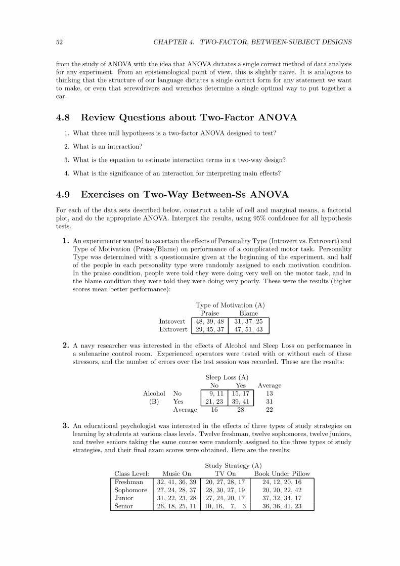
52 CHAPTER 4. TWO-FACTOR, BETWEEN-SUBJECT DESIGNS
from the study of ANOVA with the idea that ANOVA dictates a single correct method of data analysisfor any experiment. From an epistemological point of view, this is slightly naive. It is analogous tothinking that the structure of our language dictates a single correct form for any statement we wantto make, or even that screwdrivers and wrenches determine a single optimal way to put together acar.
4.8 Review Questions about Two-Factor ANOVA
1. What three null hypotheses is a two-factor ANOVA designed to test?
2. What is an interaction?
3. What is the equation to estimate interaction terms in a two-way design?
4. What is the significance of an interaction for interpreting main effects?
4.9 Exercises on Two-Way Between-Ss ANOVA
For each of the data sets described below, construct a table of cell and marginal means, a factorialplot, and do the appropriate ANOVA. Interpret the results, using 95% confidence for all hypothesistests.
1. An experimenter wanted to ascertain the effects of Personality Type (Introvert vs. Extrovert) andType of Motivation (Praise/Blame) on performance of a complicated motor task. PersonalityType was determined with a questionnaire given at the beginning of the experiment, and halfof the people in each personality type were randomly assigned to each motivation condition.In the praise condition, people were told they were doing very well on the motor task, and inthe blame condition they were told they were doing very poorly. These were the results (higherscores mean better performance):
Type of Motivation (A)Praise Blame
Introvert 48, 39, 48 31, 37, 25Extrovert 29, 45, 37 47, 51, 43
2. A navy researcher was interested in the effects of Alcohol and Sleep Loss on performance ina submarine control room. Experienced operators were tested with or without each of thesestressors, and the number of errors over the test session was recorded. These are the results:
Sleep Loss (A)No Yes Average
Alcohol No 9, 11 15, 17 13(B) Yes 21, 23 39, 41 31
Average 16 28 22
3. An educational psychologist was interested in the effects of three types of study strategies onlearning by students at various class levels. Twelve freshman, twelve sophomores, twelve juniors,and twelve seniors taking the same course were randomly assigned to the three types of studystrategies, and their final exam scores were obtained. Here are the results:
Study Strategy (A)Class Level: Music On TV On Book Under PillowFreshman 32, 41, 36, 39 20, 27, 28, 17 24, 12, 20, 16Sophomore 27, 24, 28, 37 28, 30, 27, 19 20, 20, 22, 42Junior 31, 22, 23, 28 27, 24, 20, 17 37, 32, 34, 17Senior 26, 18, 25, 11 10, 16, 7, 3 36, 36, 41, 23

4.10. ANSWERS TO EXERCISES 53
4.10 Answers to Exercises
1. Personality and Motivation.
Design:
• Factor A: Method of Motivation. 2 levels (Praise/Blame), Between-Ss.
• Factor B: Type of Personality. 2 levels (Intro/Extro), Between-Ss.
• 3 Subjects per group.
Model: Yijk = µ + Ai + Bj + ABij + S(AB)ijk
Estimation Equations:µ = Y...
Ai = Yi.. - µ
Bi = Y.j. - µ
ABij = Yij. - µ - Ai - Bj
S(AB)ijk = Yijk - µ - Ai - Bj - ABij
Decomposition Matrix:
Yijk = µ + Ai + Bj + ABij + S(AB)ijk
48 = 40 + 1 - 2 + 6 + 339 = 40 + 1 - 2 + 6 - 648 = 40 + 1 - 2 + 6 + 331 = 40 - 1 - 2 - 6 + 037 = 40 - 1 - 2 - 6 + 625 = 40 - 1 - 2 - 6 - 629 = 40 + 1 + 2 - 6 - 845 = 40 + 1 + 2 - 6 + 837 = 40 + 1 + 2 - 6 + 047 = 40 - 1 + 2 + 6 + 051 = 40 - 1 + 2 + 6 + 443 = 40 - 1 + 2 + 6 - 4
ANOVA Table:
Source df SS MS F Error Termµ 1 19,200 19,200.0 537.06 S(AB)A 1 12 12.0 0.34 S(AB)B 1 48 48.0 1.34 S(AB)AB 1 432 432.0 12.08 S(AB)S(AB) 8 286 35.8Total 12 19,978
Interpretation: Based on the Fcritical with 1 and 8 df, we see that only the baseline andAB interaction have significant effects. Regarding the former, we can conclude that themean performance is greater than zero, which is not too interesting. (This will be thelast example in which we mention an uninteresting baseline.) Regarding the latter, wecan conclude that the effect of Motivation Type is different for Introverts than Extroverts.Looking back at the cell means or factorial plot, we can conclude even more specificallythat the difference (Praise minus Blame) is greater for Introverts than Extroverts.
2. Sleep Loss and Alcohol.
Design:
• Factor A: Sleep loss. 2 levels (No/Yes), Between-Ss.
• Factor B: Alcohol. 2 levels (No/Yes), Between-Ss.
• 2 Subjects per group.
Model: Same as previous exercise.
Estimation Equations: Same as previous exercise.

54 CHAPTER 4. TWO-FACTOR, BETWEEN-SUBJECT DESIGNS
Decomposition Matrix:
Yijk = µ + Ai + Bj + ABij + S(AB)ijk
9 = 22 - 6 - 9 + 3 - 111 = 22 - 6 - 9 + 3 + 115 = 22 + 6 - 9 - 3 - 117 = 22 + 6 - 9 - 3 + 121 = 22 - 6 + 9 - 3 - 123 = 22 - 6 + 9 - 3 + 139 = 22 + 6 + 9 + 3 - 141 = 22 + 6 + 9 + 3 + 1
ANOVA Table:
Source df SS MS F Error Termµ 1 3,872 3,872 1936 S(AB)A 1 288 288 144 S(AB)B 1 648 648 324 S(AB)AB 1 72 72 36 S(AB)S(AB) 4 8 2Total 8 4888
Interpretation: Both alcohol and sleep loss tend to increase errors. Furthermore, the increasecaused by both together is more than the sum of the two increases produced by eitherstressors.
3. Class Level and Study Strategy.
Design:
• Factor A: Study Strategy. 3 levels (Music/TV/Pillow), Between-Ss.
• Factor B: Class Level. 4 levels (Fresh/Soph/Junior/Senior), Between-Ss.
• 4 Subjects per group.
Cell Means:Study Strategy (Factor A)
Class Level (B): Music On TV On Book Under Pillow AverageFreshman 37 23 18 26Sophomore 29 26 26 27Junior 26 22 30 26Senior 20 9 34 21Average 28 20 27 25
Model: Same as previous exercises.
Estimation Equations: Same as previous exercises.

4.10. ANSWERS TO EXERCISES 55
Decomposition Matrix:
Yijk = µ + Ai + Bj + ABij + S(AB)ijk
32 = 25 + 3 + 1 + 8 - 541 = 25 + 3 + 1 + 8 + 436 = 25 + 3 + 1 + 8 - 139 = 25 + 3 + 1 + 8 + 220 = 25 - 5 + 1 + 2 - 327 = 25 - 5 + 1 + 2 + 428 = 25 - 5 + 1 + 2 + 517 = 25 - 5 + 1 + 2 - 624 = 25 + 2 + 1 - 10 + 612 = 25 + 2 + 1 - 10 - 620 = 25 + 2 + 1 - 10 + 216 = 25 + 2 + 1 - 10 - 227 = 25 + 3 + 2 - 1 - 224 = 25 + 3 + 2 - 1 - 528 = 25 + 3 + 2 - 1 - 137 = 25 + 3 + 2 - 1 + 828 = 25 - 5 + 2 + 4 + 230 = 25 - 5 + 2 + 4 + 427 = 25 - 5 + 2 + 4 + 119 = 25 - 5 + 2 + 4 - 720 = 25 + 2 + 2 - 3 - 620 = 25 + 2 + 2 - 3 - 622 = 25 + 2 + 2 - 3 - 442 = 25 + 2 + 2 - 3 + 1631 = 25 + 3 + 1 - 3 + 522 = 25 + 3 + 1 - 3 - 423 = 25 + 3 + 1 - 3 - 328 = 25 + 3 + 1 - 3 + 227 = 25 - 5 + 1 + 1 + 524 = 25 - 5 + 1 + 1 + 220 = 25 - 5 + 1 + 1 - 217 = 25 - 5 + 1 + 1 - 537 = 25 + 2 + 1 + 2 + 732 = 25 + 2 + 1 + 2 + 234 = 25 + 2 + 1 + 2 + 417 = 25 + 2 + 1 + 2 - 1326 = 25 + 3 - 4 - 4 + 618 = 25 + 3 - 4 - 4 - 225 = 25 + 3 - 4 - 4 + 511 = 25 + 3 - 4 - 4 - 910 = 25 - 5 - 4 - 7 + 116 = 25 - 5 - 4 - 7 + 77 = 25 - 5 - 4 - 7 - 23 = 25 - 5 - 4 - 7 - 636 = 25 + 2 - 4 + 11 + 236 = 25 + 2 - 4 + 11 + 241 = 25 + 2 - 4 + 11 + 723 = 25 + 2 - 4 + 11 - 11

56 CHAPTER 4. TWO-FACTOR, BETWEEN-SUBJECT DESIGNS
ANOVA Table:
Source df SS MS F Error Termµ 1 30,000 30,000.0 727.76 S(AB)A 2 608 304.0 7.37 S(AB)B 3 264 88.0 2.13 S(AB)AB 6 1,576 262.7 6.37 S(AB)S(AB) 36 1,484 41.2Total 48 33,932
Interpretation: The significant Fobserved for A indicates that the three study strategies arenot all equivalent, and the significant Fobserved for AB indicates that the relative patternacross the three study strategies is not the same for all class levels. These conclusionsare a bit vague, but they are exactly what is implied by the F’s. Looking back at themarginal means for A, we see that the marginal means for Music-On and Book-Under-Pillow are about the same, both much higher than TV-On. Because we know there is areal effect here, this pattern makes it clear what the effect is: It is worst to study with theTV on. Because the interaction is significant, we should also look back at the cell meansor factorial plot. Unfortunately, there is no convenient summary of all the cells whichseems to describe the results. It appears that Freshman do especially well studying withMusic On and especially poorly with the Book Under Pillow strategy, whereas Seniors doespecially well with the Book Under Pillow and especially badly with the TV on (maybethey watch different shows). But we cannot conclude any of these things for sure withoutspecial paired comparison techniques, so we must stop with the overall conclusion thatthe pattern of strategy effects changes across class levels. Of course, we can present thefactorial plot together with this conclusion and let the readers make their own inferencesabout what caused the interaction.

Chapter 5
Three-Factor, Between-SubjectDesigns
5.1 A More General Conceptual Overview of ANOVA
Before moving on to more complicated experimental designs, it is useful to step back and consolidatethe concepts developed so far. In both one- and two-way designs, the linear model provides a way toexpress data values as the sum of a number of components:
• One-Way Model: Yij = µ + Ai + S(A)ij
• Two-Way Model: Yijk = µ + Ai + Bj + ABij + S(AB)ijk
There is an important sense in which the terms of the model are independent descriptors of thedata. They are independent in that successive terms in the model (going from left to right) measurenew effects beyond what has already been measured. Main effects, for example, are measured asdeviations from the baseline. Interactions are deviations from cell means expected on the basis of thebaseline and the main effects. Because each term is measured relative to previous terms in the model,we say that the successive terms are independent. In other words, each term is used to describe aproperty of the data not described by any previous term in the model; the terms are non-redundant.
Terms in the model can be regarded as descriptors of the data in the sense that they provide a wayof rewriting the data. We have used the linear model to form a decomposition matrix, in which eachdata score is written as the sum of a number of terms. It is possible to write out the whole set of datasimply by listing the actual scores (the numbers to the left of the equals signs in the decompositionmatrix), and it is also possible to write out the data set by listing the values of the various terms inthe linear model (the numbers to the right of the equals signs in the decomposition matrix). Since theterms in the linear model are chosen so that each data value is exactly the sum of the terms associatedwith it, the linear model is always “true” for every data point. This the sense in which the linearmodel provides us with a way of describing or rewriting the data.
What good is the linear model, if it only rewrites the data for us? The main advantage of thelinear model is that it rewrites the data in terms of independent and meaningful components: baseline,main effects, interactions, and error. For example, in the one-way design, there is a term in the modelexplicitly designed to capture the differences between groups (i.e., the effect of the factor). In thetwo-way design, there is one term for each of the two experimental factors. The main effect terms inthe two-way design are especially useful, because they measure the effect of one factor averaged overthe levels of the other factor (i.e., independent of the second factor).
As we saw in the two-way design, it is not always possible to describe the data just in terms of µ,Ai, Bj , and S(AB)ijk . An additional term, namely ABij , is needed to the extent that an interactionis present (i.e., the effect of one factor depends on the level of the other factor). In other words,an AB interaction term might be needed to describe the data, because the cell means might not beexactly predicted by the baseline, the main effect of A, and the main effect of B.
For example, in a three by three design the cell means can always be written as shown in Table 5.1.The parameter estimates will always add up to the exact cell mean. However, if the AB term weredropped from the model, it would be easy to come up with data sets for which no possible assignmentof numbers to µ, Ai, and Bj could reproduce the cell means. Thus, we need the interaction term todescribe the data.
57

58 CHAPTER 5. THREE-FACTOR, BETWEEN-SUBJECT DESIGNS
B1 B2 B3
A1 µ+A1+B1+AB11 µ+A1+B2+AB12 µ+A1+B3+AB13
A2 µ+A2+B1+AB21 µ+A2+B2+AB32 µ+A2+B3+AB23
A3 µ+A3+B1+AB31 µ+A3+B2+AB32 µ+A3+B3+AB33
Table 5.1: Model for Cell Means in 3 x 3 Design
The point of the above discussion is that various logically different types of effects can be presentin a two-factor design, and our model must allow us to measure all of them by including correspondingterms. As we consider experimental designs with more factors, we will be forced to add more andmore complicated terms to the model to measure all of the different sorts of interactions that can bepresent. These terms will be correspondingly more difficult to interpret, but that is not a flaw in themodel. It simply reflects the fact that the real world can produce very complicated patterns of data.
5.2 ANOVA Computations for Three-Factor Between-Ss Designs
Having studied between-subjects designs with one and two experimental factors, we need only slightlygeneralize our concepts to deal with between-subjects designs involving three or more factors. Thesedesigns are not much more complex than the two-way design computationally, and yet the additionof a third factor can lead to real difficulties in interpreting the results.
As an example design, we will work with a hypothetical experiment concerning the influence ofgender on sentences recommended by jurors. Imagine that the subjects are jurors in mock trials,and exactly the same evidence is presented concerning the defendant’s guilt in all conditions of theexperiment. At the end of the trial each juror is asked to recommend a prison sentence for thedefendant (0-15 years), and this number is the dependent variable. The experimental factors arethe Gender of the Juror (A), the Gender of the Defendant (B), and the Gender of the ProsecutingAttorney (C). Hypothetical data from this three-factor experiment are shown in Table 5.2, with fourobservations per cell.
Male Prosecutor: Female Prosecutor:Defendant: Defendant:
Male Female Male FemaleJuror: Male 10, 11, 10, 11 5, 4, 5, 4 Juror: Male 3, 4, 4, 3 5, 5, 6, 6
Female 4, 4, 5, 4 5, 5, 5, 6 Female 5, 5, 4, 5 6, 5, 6, 6
Table 5.2: Sample Data For Three-Way Between-Ss Design
5.2.1 ModelThe first step in the analysis is to construct the linear model, which looks like this for a three-way,between-subjects design:
Yijkl = µ + Ai + Bj + ABij + Ck + ACik + BCjk + ABCijk + S(ABC)ijkl
where,
i indicates the level of A (1 denotes male juror, 2 denotes female).
j indicates the level of B (1 denotes male defendant, 2 denotes female).
k indicates the level of C (1 denotes male prosecutor, 2 denotes female).
l indicates the subject within cell (1, 2, 3, or 4).

5.2. ANOVA COMPUTATIONS FOR THREE-FACTOR BETWEEN-SS DESIGNS 59
As in the one- and two-way designs, the model has terms for the overall baseline and for the maineffect of each experimental factor (Ai, Bj , and Ck).1 We also see three different two-way interactionterms (ABij , ACik, and BCjk), because there are three pairs of factors that might produce specialeffects in combination. Specifically, the effect of Defendant Gender may depend on Prosecutor Gender,the effect of Defendant Gender may depend on Juror Gender, or the effect of Prosecutor Gender maydepend on Juror Gender (and vice versa for each of these). The other familiar looking term in themodel is the subject error term at the end. As usual, the model allows for some error associated witheach score.
The new term in the linear model for the three-way design is the three-way interaction term,ABCijk . A three-factor interaction can be understood as an extension of the concept of a two-factorinteraction in any of several ways. First, recall that one way to think about a two-factor interactionterm was as a measurement of the extent to which the results depended on the particular pair of levelsbeing tested. Under this conception of a two-factor interaction, it measured the extent to which a cellmean differed from what would be predicted given the baseline and the two main effects. Similarly,the three-factor interaction can be thought of as measuring the extent to which the results dependon a particular combination of all three factors. In other words, the three-factor interaction measureshow much the cell means differ from what would be expected given the baseline, the main effects, andthe two-factor interactions.
Another conception of the two-factor interaction was the extent to which one factor has an effectthat depends on the level of a second factor. This conception provides a more concrete way to viewthe three-factor interaction: the extent to which a particular two-factor interaction depends on thelevel of a third factor. For example, we could think about the two-factor interaction between Genderof Juror and Gender of Prosecutor. Based on our observed results, we could plot this interactiontwice: once for male defendants and once for female defendants. The question is whether these twoplots show the same two-way interaction. If they do (i.e., if the two-factor interaction is the same atboth levels of the third factor), then there is no three-way interaction. But if the plots show a differentpattern (i.e., if the two-factor interaction is different for male defendants than for female defendants),then there is a three-way interaction.
5.2.2 Estimation
Estimation in the three-way design is a simple extension of estimation in the two-way design, andwe can now begin to formulate a general rule for estimation in any design. The exact estimationequations are shown in Table 5.3.
µ = Y....
Ai = Yi...-µ
Bj = Y.j..-µ
ABij = Yij..-µ-Ai-Bj
Ck = Y..k.-µ
ACik = Yi.k.-µ-Ai-Ck
BCjk = Y.jk.-µ-Bj-Ck
ABCijk = Yijk.-µ-Ai-Bj-ABij - Ck-ACik-BCjk
S(ABC)ijkl = Yijkl-µ-Ai-Bj-ABij- Ck-ACik-BCjk-ABCijk
= Yijkl - Yijk.
Table 5.3: Estimation Equations for Three-Way Between-Ss ANOVA
The general pattern of the estimation process works from left to right across the linear model, justas it did in the one- and two-way designs. To estimate µ, we use the grand mean across all the data.The only change from the simpler designs is that the grand mean is obtained by averaging across moreexperimental factors. These factors have their own terms in the model, however, so the existence ofthese factors does not change the estimate of µ.
1The terms in a linear model can be written in any order. In this course, we will use an ordering principle designedto make it easy to construct the model, described in section 6.1.1. This principle does not keep all the main effectstogether, all the two-way interactions together, and so on. That is a price we will pay.

60 CHAPTER 5. THREE-FACTOR, BETWEEN-SUBJECT DESIGNS
As in the one- and two-way designs, the main effect term associated with a particular level of afactor is estimated as the difference between the average of all scores at that level of the factor minusthe baseline. The only change from the simpler designs is that there are more factors to average acrossto get the mean for the specified level.
The estimates of the two-factor interaction terms are also computed just as they were in thetwo-way design, except that there is again an extra subscript to average over. Again, the two-factorinteraction effect associated with a particular pair of levels is estimated by taking the mean at thatcombination of levels, and then subtracting the baseline and the main effect terms corresponding tothose two levels. As discussed above, a change from the two-way design is that now we have threetwo-way interactions instead of just one, because there are three possible pairs of factors.
In a three-way design, there is an estimated three-way interaction term for each cell in the design.The estimated value for a cell is the cell mean minus that which is explained by the baseline, the maineffects, and the two-way interactions. Whatever is not explained by those terms is a special effectdue to the three-way combination of levels at that cell. As is discussed extensively below, it can beinterpreted as a change in one of the two-factor interactions depending on the level of the third factor.
Finally, an estimate of S(ABC)ijkl is obtained for each data value. As in previous designs, thiserror term is estimated as the score minus all those parts of the score explained by other termsin the model. Again, one can think of the error as whatever the model needs to come out right. Acomputationally simpler way to get the estimates of S(ABC)ijkl is to take the difference between eachscore and its cell mean. We will not emphasize this method, however, because it does not generalizewell to within-subjects designs. The notion of error as something unexplained by other terms in themodel generalizes better.
Before attempting to use the estimation equations to break down the individual scores, it is usefulto calculate all the cell and marginal means, as shown in Table 5.4. It is easiest to begin by computingthe cell means. From these, compute all the possible two-way tables of marginal means by averagingout one factor at a time. For example, the marginal table for the juror by defendant interaction isobtained by averaging across male and female prosecutors at each possible combination of gender ofjuror and gender of defendant. After we have all the two-way tables, we compute the marginal meansfor the main effects and the overall mean.
Cell Means: (Yijk.)Male Prosecutors: Female Prosecutors:
Defendant: Defendant:Male Female Male Female
Juror: Male 10.50 4.50 Juror: Male 3.50 5.50Female 4.25 5.75 Female 4.75 5.75
Marginal Means:Yij.. Yi.k. Y.jk.
Defendant Prosecutor ProsecutorMale Female Male Female Male Female
Jur: Male 7.0 5.0 Jur: Male 7.5 4.5 Def: Male 7.375 4.125Fem. 4.5 5.5 Fem. 4.75 5.25 Fem. 4.875 5.625
Jurors: Yi... Male = 6.000, Female = 5.000Defendants: Y.j.. Male = 5.750, Female = 5.250Prosecutors: Y..k. Male = 6.125, Female = 4.875Grand Mean: Y.... 5.500
Table 5.4: Cell and Marginal Means for Mock Jury Experiment
5.2.3 Decomposition Matrix and SS’s
With the estimation equations and the cell and marginal means, it is easy (though tedious) to do allof the computation necessary to arrive at the decomposition matrix shown in Table 5.5.
Once we have the decomposition matrix, we can start to write down the ANOVA table, shown inTable 5.6. As always, there is one source line for each term in the linear model. The sum of squares foreach term can be computed by squaring and totaling the corresponding column of the decompositionmatrix, as always.

5.2. ANOVA COMPUTATIONS FOR THREE-FACTOR BETWEEN-SS DESIGNS 61
Yijkl = µ + Ai + Bj + Cij + ABk + ACik + BCjk + ABCijk + S(ABC)ijkl
10 = 5.5 + 0.5 + 0.25 + 0.625 + 0.75 + 0.875 + 1 + 1 − 0.511 = 5.5 + 0.5 + 0.25 + 0.625 + 0.75 + 0.875 + 1 + 1 + 0.510 = 5.5 + 0.5 + 0.25 + 0.625 + 0.75 + 0.875 + 1 + 1 − 0.511 = 5.5 + 0.5 + 0.25 + 0.625 + 0.75 + 0.875 + 1 + 1 + 0.53 = 5.5 + 0.5 + 0.25 − 0.625 + 0.75 − 0.875 − 1 − 1 − 0.54 = 5.5 + 0.5 + 0.25 − 0.625 + 0.75 − 0.875 − 1 − 1 + 0.54 = 5.5 + 0.5 + 0.25 − 0.625 + 0.75 − 0.875 − 1 − 1 + 0.53 = 5.5 + 0.5 + 0.25 − 0.625 + 0.75 − 0.875 − 1 − 1 − 0.55 = 5.5 + 0.5 − 0.25 + 0.625 − 0.75 + 0.875 − 1 − 1 + 0.54 = 5.5 + 0.5 − 0.25 + 0.625 − 0.75 + 0.875 − 1 − 1 − 0.55 = 5.5 + 0.5 − 0.25 + 0.625 − 0.75 + 0.875 − 1 − 1 + 0.54 = 5.5 + 0.5 − 0.25 + 0.625 − 0.75 + 0.875 − 1 − 1 − 0.55 = 5.5 + 0.5 − 0.25 − 0.625 − 0.75 − 0.875 + 1 + 1 − 0.55 = 5.5 + 0.5 − 0.25 − 0.625 − 0.75 − 0.875 + 1 + 1 − 0.56 = 5.5 + 0.5 − 0.25 − 0.625 − 0.75 − 0.875 + 1 + 1 + 0.56 = 5.5 + 0.5 − 0.25 − 0.625 − 0.75 − 0.875 + 1 + 1 + 0.54 = 5.5 − 0.5 + 0.25 + 0.625 − 0.75 − 0.875 + 1 − 1 − 0.254 = 5.5 − 0.5 + 0.25 + 0.625 − 0.75 − 0.875 + 1 − 1 − 0.255 = 5.5 − 0.5 + 0.25 + 0.625 − 0.75 − 0.875 + 1 − 1 + 0.754 = 5.5 − 0.5 + 0.25 + 0.625 − 0.75 − 0.875 + 1 − 1 − 0.255 = 5.5 − 0.5 + 0.25 − 0.625 − 0.75 + 0.875 − 1 + 1 + 0.255 = 5.5 − 0.5 + 0.25 − 0.625 − 0.75 + 0.875 − 1 + 1 + 0.254 = 5.5 − 0.5 + 0.25 − 0.625 − 0.75 + 0.875 − 1 + 1 − 0.755 = 5.5 − 0.5 + 0.25 − 0.625 − 0.75 + 0.875 − 1 + 1 + 0.255 = 5.5 − 0.5 − 0.25 + 0.625 + 0.75 − 0.875 − 1 + 1 − 0.255 = 5.5 − 0.5 − 0.25 + 0.625 + 0.75 − 0.875 − 1 + 1 − 0.255 = 5.5 − 0.5 − 0.25 + 0.625 + 0.75 − 0.875 − 1 + 1 − 0.256 = 5.5 − 0.5 − 0.25 + 0.625 + 0.75 − 0.875 − 1 + 1 + 0.756 = 5.5 − 0.5 − 0.25 − 0.625 + 0.75 + 0.875 + 1 − 1 + 0.255 = 5.5 − 0.5 − 0.25 − 0.625 + 0.75 + 0.875 + 1 − 1 − 0.756 = 5.5 − 0.5 − 0.25 − 0.625 + 0.75 + 0.875 + 1 − 1 + 0.256 = 5.5 − 0.5 − 0.25 − 0.625 + 0.75 + 0.875 + 1 − 1 + 0.25
Table 5.5: Decomposition Matrix for Mock Jury Experiment
5.2.4 Degrees of Freedom
To fill in the column for degrees of freedom, we need only reapply the rules already learned.
• The df for the mean is 1.
• The df for any main effect is the number of levels of the factor minus 1.
• The df for any interaction (including three-factor) is found by multiplying together the df’s forthe factors involved in the interaction. This multiplication rule holds true even for the higher-wayinteractions: multiply together the df’s for all the factors involved in the interaction.
• The df for S(ABC) can be found with either of two methods. Since the total df is known toequal the number of observations, the df for S(ABC) can be found by subtraction once the restof the df’s are known. Alternatively, this df can be found using the formula:
dfS(ABC) = Number of subjects - Number of groupsAs in the two-factor between-Ss design, the number of groups is the number of cells in the
design.
5.2.5 ANOVA Table
Computation of MS’s and F’s is easy once we get this far. The MS for any line of the table is theSS for that line divided by the df for that line. The F for any line is the MS for that line divided byMSS(ABC). All that remains is to look up the Fcritical for the appropriate df’s—in this case 1 and24, yielding 4.26. Now the computations are done, and the remaining problem is interpretation of theresults.

62 CHAPTER 5. THREE-FACTOR, BETWEEN-SUBJECT DESIGNS
Source df SS MS F Error Termµ 1 968.0 968.0 3318.8 S(ABC)A (Juror) 1 8.0 8.0 27.4 S(ABC)B (Defendant) 1 2.0 2.0 6.857 S(ABC)AB 1 18.0 18.0 61.7 S(ABC)C (Prosecutor) 1 12.5 12.5 42.8 S(ABC)AC 1 24.5 24.5 84.0 S(ABC)BC 1 32.0 32.0 109.7 S(ABC)ABC 1 32.0 32.0 109.7 S(ABC)S(ABC) 24 7.0 0.2917Total 32 1104.0
Table 5.6: ANOVA Table for Mock Jury Experiment
5.3 Interpreting Three-Factor ANOVAs
The general approach to interpreting the results is to proceed down the ANOVA table, saying whateach significant effect or interaction means. The initial interpretation can be general, like “there isan effect of Factor A” or “the effect of Factor A depends on the level of Factor B.” A more specificinterpretation should then be developed by examining the data and stating, in the general terms ofthe ANOVA tests, exactly what the effect is and/or how it depends on another factor. We illustratethis approach below by discussing the data analyzed in Section 5.2. Of course, it is often desirable toperform further analyses in order to make more specific statements about the results.
The significant main effects of Gender of Juror, Gender of Defendant, and Gender of Prosecutorindicate that the observed differences in marginal means for these factors were not simply due tochance. Looking at the means, then, we can interpret these F’s as indicating that: 1) On average, malejurors give longer sentences than female jurors, 2) On average, male defendants get longer sentencesthan female defendants, and 3) On average, longer sentences are given when the prosecutor is malethan female. The “on average” qualification is critically important, however. Significant higher-orderinteractions indicate that the pattern of results is more complicated than we can describe using simplestatements about main effects. Given these interactions, it is certain that the effects of some factorsdepended on the levels of some other factors, so any overall statements about the effects of thesefactors will be oversimplified.
To interpret two-way interactions properly, it is advisable to look at the marginal means or factorialplots associated with the two-way interactions. Each significant interaction says that, on average, theeffect of one factor depends on the level of the other factor, but that statement is simply too generalto be an interesting conclusion. Note that the qualification “on average” crops up again. There werethree factors in the experiment, and each two-way interaction is an average across the levels of thethird factor. Since the three-way interaction was significant, though, we know that each two-wayinteraction changes depending on the level of the third factor. Any conclusion about the interactionmust take this averaging into account. Just as we were forced to be cautious in our interpretationsof main effects if there were significant two-way interactions, so too are we forced to qualify ourinterpretations of the two-way interactions when there is a significant three-way interaction.
In practice, it is much easier to understand an interaction when it is graphed than when it ispresented in a table of means. The three panels in Figure 5.1 show graphs of the means associatedwith each of the two-way interactions observed in this experiment, and our interpretations are reallylittle more than descriptions of these graphs.
The Gender of Juror by Gender of Defendant interaction in Panel A arises because sentences arelonger overall when the defendant and juror are the same gender than when they are opposite genders.It appears that, overall, male jurors give much longer sentences to male defendants than to femaledefendants, while female jurors are slightly more severe with female defendants than with male ones.Alternatively, one could view the interaction as male defendants getting longer sentences, overall, frommale jurors than from female jurors, while female defendants get longer sentences, overall, from femalejurors than male jurors. Neither of these two conclusions is strictly justified without more specificanalyses, because both make statements about specific means that are really only part of the totalinteraction (e.g., “male jurors give longer sentences to male defendants than to female defendants”).To come up with a proper interpretation, the conclusion must somehow refer to the whole interaction,as did the original conclusion relying on same vs. different gender.

5.3. INTERPRETING THREE-FACTOR ANOVAS 63
Male FemaleDefendant
4
5
6
7
8
Sen
tenc
e
AMale Jurors
Female Jurors
Male FemaleProsecutor
4
5
6
7
8 B Male Defendants
FemaleDefendants
Male FemaleProsecutor
4
5
6
7
8 C Male Jurors
Female Jurors
Figure 5.1: Sentence as a function of genders of A) defendant and juror; B) defendant and prosecutor;and C) prosecutor and juror.
The other two two-way interactions also reflect an overall tendency toward longer sentences inthe same-gender combinations than in the opposite-gender combinations, as can be seen by studyingPanels B and C. Conclusions about these interactions would be analogous to those drawn from theGender of Juror by Gender of Defendant interaction.
The interaction that is really difficult to interpret is the three-way. Two different strategies areavailable for trying to understand the nature of the interaction, but neither one is guaranteed to givea really clear picture. Sometimes, you end up just concluding that there is something complicatedgoing on that you can’t understand.2
If you do use one strategy and find that it leads you to a satisfactory interpretation, it is stillworthwhile to try the other strategy. After all, interactions can be looked at in many different ways.The more different points of view we take in considering an interaction, the better chance we have offully understanding all its implications.
5.3.1 Strategy 1: How does a two-way interaction change?
The first strategy is to focus your point of view on a particular two-way interaction (any one youlike– you can try it from all points of view to see which makes the most sense). Graph this two-wayinteraction separately for each level of the third factor. For example, Figure 5.2 shows the Gender ofJuror by Gender of Defendant interaction graphed separately for male and female prosecutors.
Male FemaleDefendant
2
4
6
8
10
12
Sen
tenc
e
Male Prosecutors
AMale Jurors
Female Jurors
Male FemaleDefendant
2
4
6
8
10
12
Female Prosecutors
B
Male Jurors
Female Jurors
Figure 5.2: Sentence as a function of defendant and juror genders, separately for male and femaleprosecutors.
The significant three-way interaction indicates that the interaction is not the same in these twographs. Can you see the difference? In Figure 5.2 it appears that there is a bigger difference in slopes
2This conclusion is not all that uncommon in published scientific articles. Usually the article will have contributedsome new piece of information with a clear theoretical significance, but there will be other aspects of the data thatremain unexplained.

64 CHAPTER 5. THREE-FACTOR, BETWEEN-SUBJECT DESIGNS
for the male prosecutors than for the female prosecutors. Notice also that the Gender of Juror byGender of Defendant interactions go in opposite directions with male and female prosecutors. Withmale prosecutors, the observed average sentences were longer when the juror and defendant werethe same gender, while with female prosecutors the observed average sentences were longer when thejuror and the defendant were opposite genders. While we cannot conclude that the true means exactlyfollow the pattern of the observed averages (note that we have made statements comparing particularcells, rather than sticking to a summary of the total interaction pattern), we can conclude that theinteraction of Gender of Juror with Gender of Defendant is different when the prosecutor is male thanwhen the prosecutor is female.
That last conclusion might make sense to someone schooled in ANOVA, but what if we wantedto interpret the three-way interaction for a layperson? We might be able to communicate the ideaby saying that, with male prosecutors more than with female prosecutors, sentences are longer whenthe juror and defendant are the same gender as opposed to opposite genders. You can illustrate thisstatement with a table like 5.7. The value in the table is the size of the Gender of Juror by Gender ofDefendant interaction: average sentences with (same gender juror and defendant) - average sentenceswith (opposite gender juror and defendant). Clearly, this difference is larger with male than femaleprosecutors.
Prosecutor Size of Interaction
Male: 10.5+5.752 − 4.5+4.25
2 = 3.75
Female: 3.5+5.752 − 5.5+4.75
2 = −0.5
Table 5.7: Effect of Prosecutor on Juror By Defendant Interaction
We may be able to make other interesting statements about these results by repeating this processfocusing on one of the other pairwise interactions.
5.3.2 Strategy 2: How does a main effect change?
Another way to look at a three-way interaction is to focus on a main effect, and see how that maineffect depends on the interaction of the other two factors. This new strategy looks at one particularmain effect as a function of the factorial design defined by the other two factors.
For example, look at the difference between sentences given to male and female defendants (say,male minus female). From the cell means, we can compute this difference for each possible combinationof male and female jurors and prosecutors. A graph of the results is shown in Figure 5.3. The verticalaxis measures the size of the Gender of Defendant effect, which we might be tempted to call a “bias”against male defendants, since the experiment involved identical evidence in all conditions. The Genderof Defendant effect (“anti-male bias,” if you will) is shown for each gender of juror and prosecutor.
Male FemaleProsecutor
-2
0
2
4
6
Ant
i-mal
eB
ias
Male Jurors
Female Jurors
Figure 5.3: Bias against male defendants as a function of juror and prosecutor genders.
Inspecting Figure 5.3 gives a slightly new view on the three-way interaction, and shows howwe should qualify our interpretation of the overall Gender of Defendant effect (males get longer

5.4. EXERCISES: THREE-FACTOR, BETWEEN-SS ANOVA 65
sentences than females). First of all, note that the significant overall main effect of Gender ofDefendant corresponds to the fact that the average of the four points plotted on this figure is above 0.Interestingly, though the average is above 0, only one of the four points is actually above 0. Thus theoverall anti-male defendant bias is the result of a big bias in one condition rather than a consistentbias across all conditions. Furthermore, we can see that Gender of Juror and Gender of Prosecutorproduce both main effects and an interactive effect on this bias. The fact that the bias is bigger overallfor male jurors than for female jurors reflects the Gender of Juror by Gender of Defendant interaction.The fact that the bias is bigger overall with male prosecutors than with female prosecutors reflectsthe Gender of Prosecutor by Gender of Defendant interaction.
5.3.3 Summary
It is clear by now that three-way interactions can be very difficult to understand and describeintuitively. It may be especially difficult to figure out how to start looking at a three-way interaction.Is it better to start with strategy 1 or 2? Whichever strategy you use, how do you know whichinteraction or main effect to focus on?
There are no general statistical answers to such questions. In some situations the experimenterwill have a strong theoretical interest in some particular main effect or interaction, and that willdetermine which point of view to adopt. In other situations there will be no particular reason toadopt one point of view rather than another. In both cases the careful researcher will look at aninteraction from several, maybe even all possible points of view. The only cost of trying a new pointof view is researcher time, and the potential payoff is an important insight into what is going on inthe experiment. If that potential payoff is not exciting enough to justify the extra effort, then theresearcher ought to look for an easier way to make a living.
5.4 Exercises: Three-Factor, Between-Ss ANOVA
1. A nutritionist was interested in the determining the benefit produced by having different combinationsof three different amino acids (A, B, and C) in the diet. He randomly divided 24 rats into the8 groups shown below. Each rat was fed a diet including the indicated combination of aminoacids, and the life span of the rat was measured, with the results shown in the table. Performthe ANOVA and interpret the results.
B Absent: B Present:A Absent A Present A Absent A Present
C Absent: 104 104 152 60 102 54 91 81 38 114 90 126C Present: 51 87 72 114 130 74 134 115 99 122 118 168
2. The educational psychologist interested in three study strategies (see exercises for Two-WayBetween-Ss Designs) decided to add Student Gender as a third factor (Factor A: 1 = Female,2 = Male) in a repetition of the study with two subjects per cell. The new results are shownbelow; what do they suggest?
A1 A2C1 C2 C3 C4 C1 C2 C3 C4
B1: 5 5 5 7 8 6 8 12 6 0 6 2 5 5 11 5B2: 13 11 13 17 18 16 25 23 4 4 2 4 7 7 9 3B3: 13 13 17 13 7 11 24 22 12 10 5 5 8 10 22 16

66 CHAPTER 5. THREE-FACTOR, BETWEEN-SUBJECT DESIGNS
5.5 Answers to Exercises
1.
Design:
• 2 x 2 x 2, Between-Ss, with 3 subjects per group.
• Factor A = absence/presence of amino acid a in diet.
• Factor B = absence/presence of amino acid b in diet.
• Factor C = absence/presence of amino acid c in diet.
• DV= Length of life of rat, in months.
Cell Means:B Absent: B Present:
A Absent A Present A Absent A PresentC Absent: 120 72 70 110C Present: 70 106 116 136
Marginal Means:
Averaged across A:B Absent B Present Average
C Absent: 96 90 93C Present: 88 126 107
Average: 92 108 100
Averaged across B:A Absent A Present Average
C Absent: 95 91 93C Present: 93 121 107
Average: 94 106 100
Averaged across C:A Absent A Present Average
B Absent: 95 89 92B Present: 93 123 108
Average: 94 106 100
Estimation equations: See Table 5.3.

5.5. ANSWERS TO EXERCISES 67
Decomposition Matrix:
Yijkl = µ + Ai + Bj + ABij + Ck + ACik + BCjk + ABCijk + S(ABC)ijkl
104 = 100 - 6 - 8 + 9 - 7 + 8 + 11 + 13 - 16104 = 100 - 6 - 8 + 9 - 7 + 8 + 11 + 13 - 16152 = 100 - 6 - 8 + 9 - 7 + 8 + 11 + 13 + 3260 = 100 + 6 - 8 - 9 - 7 - 8 + 11 - 13 - 12
102 = 100 + 6 - 8 - 9 - 7 - 8 + 11 - 13 + 3054 = 100 + 6 - 8 - 9 - 7 - 8 + 11 - 13 - 1891 = 100 - 6 + 8 - 9 - 7 + 8 - 11 - 13 + 2181 = 100 - 6 + 8 - 9 - 7 + 8 - 11 - 13 + 1138 = 100 - 6 + 8 - 9 - 7 + 8 - 11 - 13 - 32
114 = 100 + 6 + 8 + 9 - 7 - 8 - 11 + 13 + 490 = 100 + 6 + 8 + 9 - 7 - 8 - 11 + 13 - 20
126 = 100 + 6 + 8 + 9 - 7 - 8 - 11 + 13 + 1651 = 100 - 6 - 8 + 9 + 7 - 8 - 11 - 13 - 1987 = 100 - 6 - 8 + 9 + 7 - 8 - 11 - 13 + 1772 = 100 - 6 - 8 + 9 + 7 - 8 - 11 - 13 + 2
114 = 100 + 6 - 8 - 9 + 7 + 8 - 11 + 13 + 8130 = 100 + 6 - 8 - 9 + 7 + 8 - 11 + 13 + 2474 = 100 + 6 - 8 - 9 + 7 + 8 - 11 + 13 - 32
134 = 100 - 6 + 8 - 9 + 7 - 8 + 11 + 13 + 18115 = 100 - 6 + 8 - 9 + 7 - 8 + 11 + 13 - 199 = 100 - 6 + 8 - 9 + 7 - 8 + 11 + 13 - 17
122 = 100 + 6 + 8 + 9 + 7 + 8 + 11 - 13 - 14118 = 100 + 6 + 8 + 9 + 7 + 8 + 11 - 13 - 18168 = 100 + 6 + 8 + 9 + 7 + 8 + 11 - 13 + 32
ANOVA:
Source df SS MS F Error Termµ 1 240000.0 240000.0 398.423 S(ABC)A 1 864.0 864.0 1.434 S(ABC)B 1 1536.0 1536.0 2.550 S(ABC)AB 1 1944.0 1944.0 3.227 S(ABC)C 1 1176.0 1176.0 1.952 S(ABC)AC 1 1536.0 1536.0 2.550 S(ABC)BC 1 2904.0 2904.0 4.821 S(ABC)ABC 1 4056.0 4056.0 6.733 S(ABC)S(ABC) 16 9638.0 602.4Total 24 263654.0
Interpretation: First look at the significant BC interaction. It is clear that there is a mutualfacilitation when both these amino acids are present, because there is one value in the BCmarginal means that is much higher than all the others (126). (Technically, we do need todo paired comparisons to establish this, but the data are so clear-cut that in practice fewwould quarrel with the conclusion.)
Given that the BC interaction was significant, it seems reasonable to start by looking atthe ABC interaction in terms of how the BC interaction changes across levels of A. Here,we find a pattern that is startling in terms of how we believe amino acids work. With Apresent, there is a big mutual facilitation of B and C, just as we concluded from looking atthe simple BC interaction. But with A absent, the largest effect is that you should haveeither both or neither of B and C, but not one or the other. This suggests that there issomething positively harmful about having just one of the three amino acids. We don’tknow if that is a realistic possibility or not, but that is what these (fake) data suggest.
2. Design: 2 x 3 x 4, Between-Ss, with 2 Ss per group.

68 CHAPTER 5. THREE-FACTOR, BETWEEN-SUBJECT DESIGNS
Cell Means:A1 A2
C1 C2 C3 C4 C1 C2 C3 C4B1 5 6 7 10 3 4 5 8B2 12 15 17 24 4 3 7 6B3 13 15 9 23 11 5 9 19
Marginal Means:
A1 A2B1 7 5B2 17 5B3 15 11
C1 C2 C3 C4A1 10 12 11 19A2 6 4 7 11
C1 C2 C3 C4B1 4 5 6 9B2 8 9 12 15B3 12 10 9 21

5.5. ANSWERS TO EXERCISES 69
Decomposition Matrix:
Yijkl = µ + Ai + Bj + ABij + Ck + ACik + BCjk + ABCijk + S(ABC)ijkl
5 = 10 + 3 - 4 - 2 - 2 - 1 + 0 + 1 + 05 = 10 + 3 - 4 - 2 - 2 - 1 + 0 + 1 + 06 = 10 - 3 - 4 + 2 - 2 + 1 + 0 - 1 + 30 = 10 - 3 - 4 + 2 - 2 + 1 + 0 - 1 - 3
13 = 10 + 3 + 1 + 3 - 2 - 1 - 1 - 1 + 111 = 10 + 3 + 1 + 3 - 2 - 1 - 1 - 1 - 14 = 10 - 3 + 1 - 3 - 2 + 1 - 1 + 1 + 04 = 10 - 3 + 1 - 3 - 2 + 1 - 1 + 1 + 0
13 = 10 + 3 + 3 - 1 - 2 - 1 + 1 + 0 + 013 = 10 + 3 + 3 - 1 - 2 - 1 + 1 + 0 + 012 = 10 - 3 + 3 + 1 - 2 + 1 + 1 + 0 + 110 = 10 - 3 + 3 + 1 - 2 + 1 + 1 + 0 - 15 = 10 + 3 - 4 - 2 - 2 + 1 + 1 - 1 - 17 = 10 + 3 - 4 - 2 - 2 + 1 + 1 - 1 + 16 = 10 - 3 - 4 + 2 - 2 - 1 + 1 + 1 + 22 = 10 - 3 - 4 + 2 - 2 - 1 + 1 + 1 - 2
13 = 10 + 3 + 1 + 3 - 2 + 1 + 0 - 1 - 217 = 10 + 3 + 1 + 3 - 2 + 1 + 0 - 1 + 22 = 10 - 3 + 1 - 3 - 2 - 1 + 0 + 1 - 14 = 10 - 3 + 1 - 3 - 2 - 1 + 0 + 1 + 1
17 = 10 + 3 + 3 - 1 - 2 + 1 - 1 + 2 + 213 = 10 + 3 + 3 - 1 - 2 + 1 - 1 + 2 - 25 = 10 - 3 + 3 + 1 - 2 - 1 - 1 - 2 + 05 = 10 - 3 + 3 + 1 - 2 - 1 - 1 - 2 + 08 = 10 + 3 - 4 - 2 - 1 - 1 + 1 + 1 + 16 = 10 + 3 - 4 - 2 - 1 - 1 + 1 + 1 - 15 = 10 - 3 - 4 + 2 - 1 + 1 + 1 - 1 + 05 = 10 - 3 - 4 + 2 - 1 + 1 + 1 - 1 + 0
18 = 10 + 3 + 1 + 3 - 1 - 1 + 2 + 0 + 116 = 10 + 3 + 1 + 3 - 1 - 1 + 2 + 0 - 17 = 10 - 3 + 1 - 3 - 1 + 1 + 2 + 0 + 07 = 10 - 3 + 1 - 3 - 1 + 1 + 2 + 0 + 07 = 10 + 3 + 3 - 1 - 1 - 1 - 3 - 1 - 2
11 = 10 + 3 + 3 - 1 - 1 - 1 - 3 - 1 + 28 = 10 - 3 + 3 + 1 - 1 + 1 - 3 + 1 - 1
10 = 10 - 3 + 3 + 1 - 1 + 1 - 3 + 1 + 18 = 10 + 3 - 4 - 2 + 5 + 1 - 2 - 1 - 2
12 = 10 + 3 - 4 - 2 + 5 + 1 - 2 - 1 + 211 = 10 - 3 - 4 + 2 + 5 - 1 - 2 + 1 + 35 = 10 - 3 - 4 + 2 + 5 - 1 - 2 + 1 - 3
25 = 10 + 3 + 1 + 3 + 5 + 1 - 1 + 2 + 123 = 10 + 3 + 1 + 3 + 5 + 1 - 1 + 2 - 19 = 10 - 3 + 1 - 3 + 5 - 1 - 1 - 2 + 33 = 10 - 3 + 1 - 3 + 5 - 1 - 1 - 2 - 3
24 = 10 + 3 + 3 - 1 + 5 + 1 + 3 - 1 + 122 = 10 + 3 + 3 - 1 + 5 + 1 + 3 - 1 - 122 = 10 - 3 + 3 + 1 + 5 - 1 + 3 + 1 + 316 = 10 - 3 + 3 + 1 + 5 - 1 + 3 + 1 - 3

70 CHAPTER 5. THREE-FACTOR, BETWEEN-SUBJECT DESIGNS
ANOVA:
Source df SS MS F Error Termµ 1 4800.0 4800.0 886.154 S(ABC)A 1 432.0 432.0 79.754 S(ABC)B 2 416.0 208.0 38.400 S(ABC)AB 2 224.0 112.0 20.677 S(ABC)C 3 408.0 136.0 25.108 S(ABC)AC 3 48.0 16.0 2.954 S(ABC)BC 6 128.0 21.3 3.938 S(ABC)ABC 6 64.0 10.7 1.969 S(ABC)S(ABC) 24 130.0 5.4Total 48 6650.0
Interpretation: The significant sources are A, B, C, AB, and BC. Overall, we see that femalesscore better than males, the Music-On strategy is worse than the other two, and seniorsscore higher than the other classes. The advantage for females over males is especiallylarge with the TV-On strategy, intermediate with the Book Under Pillow strategy, andsmallest (possibly nonexistent) with the Music On strategy (AB interaction). The threedifferent strategies show different patterns of results across class level (BC interaction).The Music-On strategy is least affected by class level, and Book Under Pillow is mostaffected. Also, whereas test scores increase from freshmen to juniors with the Music Onand TV On strategies, they decrease with the Book Under Pillow strategy (further analysisis needed to see if this differential class effect is statistically significant). The theoreticalimplications of this pattern are not immediately apparent.

Chapter 6
Generalization of Between-SubjectDesigns
In the preceding sections, we have considered in detail ANOVA for between-subjects designs withequal sizes having one, two, or three experimental factors. ANOVA can also be used with designshaving four, five, ten, or (in principle) any number of factors. However, it would be both infinitelytedious and unnecessary to work step-by-step through an example of each size design. Instead, wecan formulate a set of general rules for computing ANOVA given an equal-cell-size, between-subjectsdesign with any number of factors. Many of these general rules will also apply to within-subjects andmixed designs.
While studying ANOVA for one, two, and three factor designs, you may have noticed a patternemerging; a similarity in the steps required to perform each ANOVA:
1. Identify the experimental factors.
2. Construct the appropriate linear model.
3. Estimate the components of the model.
4. Compute SS’s and df’s associated with each term in the model.
5. Compute MS’s and F’s.
6. Interpret the significant F’s.
These six steps constitute a general algorithm for computing ANOVA for an experimental designhaving any number of factors. This chapter presents a general explanation of the correct way toperform steps 2 through 6 (step 1 is self-explanatory) for between-subjects designs. Careful studyof this material should not only provide you with the tools necessary to perform ANOVA on datafrom any arbitrary between-subjects experimental design, but should also help you to see the materialpresented earlier as part of an orderly and coherent system.
6.1 Constructing the model
The linear model describes a data point as the sum of logically different sources of variance thatcontribute to that data value, so the appropriate model must contain a term for each source of variance.Very simply, the model must contain a term for the baseline, a term for each main effect, a term foreach interaction, and a term for error. Formally, the linear model for an N-factor between-subjectsdesign is always of the form:
Y = µ + main effects + 2-way interactions + 3-way interactions+ ... + N-way interaction + S(Between-Ss factors)
leaving off the subscripts for simplicity.There is always one main effect term for each experimental factor, one 2-way interaction term for
each pair of factors, one 3-way interaction term for each combination of three factors, etc. Counting
71

72 CHAPTER 6. GENERALIZATION OF BETWEEN-SUBJECT DESIGNS
the µ and error terms, there are a total of 2N +1 terms in the linear model for a design with N factors.For example, a four-factor design will have the following linear model:
Yijklm = µ + Ai + Bj + Ck + Dl + ABij + ACik + ADil + BCjk + BDjl + CDkl
+ ABCijk + ABDijl + ACDikl + BCDjkl + ABCDijkl + S(ABCD)ijklm
As stated above, a correct linear model should contain 2N +1 terms. This fact can be used to insurethat no terms have been omitted from the model. In the four factor example above, we should have24 + 1 = 17 terms on the right-hand side of the equals sign, as in fact we do. This is an encouraging,but not conclusive sign. We must also be sure that the terms in the model are all correct. Great caremust be exercised in construction of the linear model, as it is the model that determines all subsequentcalculations.1
6.1.1 The Order of the Terms in the Model
Although it seems most natural to write out the model with the terms arranged as shown above (allmain effects, then all two-way interactions, then all three-way interactions, etc.), it is easier to generatethe correct model using a strategy that puts the terms down in another order, and so we will actuallyuse this alternate ordering of terms.
This strategy starts with the terms for baseline, the first two main effects, and their interaction,like this:
Y = µ + Ai + Bj + ABij
To this starting model, you add the next main effect (Ck). Then go back to the first main effect andform an interaction of this new main effect with each previous term in the model. At the beginning ofthe model we find the A term, and so we form its interaction with C to get AC. After A in the modelcomes B, so we next form the BC interaction. After B in the model comes AB, so we next form theABC interaction. That brings us back to the factor we are adding (C), so we are done with this step.Here is the result obtained so far, with the terms generated by adding the C factor written directlybelow their “matching” terms from the earlier part of the model:
Y = µ + Ai + Bj + ABij +Ck + ACik + BCjk + ABCijk
Of course, stringing all the terms out on a single line, the model constructed so far looks like this:
Y = µ + Ai + Bj + ABij + Ck + ACik + BCjk + ABCijk
To add another factor D, we repeat the process. First, add D on the end of the model. Then, goback to the A term at the beginning and proceed rightward forming interactions of D with each termalready in the model, resulting in AD, BD, ABD, CD, etc, as shown below.
Y = µ +Ai +Bj +ABij +Ck +ACik +BCjk +ABCijk
Dl +ADil +BDjl +ABDijl +CDkl +ACDikl +BCDjkl +ABCDijkl
To add another factor E, we repeat the process. Put the E on the end. Go back to the A termand form interactions of E with each term already in the model.
The process can be repeated for each new factor to add indefinitely many factors. Note that themodel doubles in size each time we add a factor, because we get not only a new main effect butan interaction with all the previous terms in the model. This means that the model starts to have
1For those students with some background in probability or combinatorics, note that the interaction terms in themodel comprise the set of all possible combinations of size K from a set of size N for K equal 2 to N. That is, the two-wayinteraction terms are the set of all pairs of size two from N items; the three-way interaction terms are all combinationsof size three, etc. The number of such combinations for a given K is “N-choose-K”, computed as
(NK
)=
N !
K! × (N − K)!
Computing N-choose-K for each K can provide a further check on the accuracy of your linear model, as it will indicatethe correct number of terms for each size interaction. In the above example, 4-choose-2 equals 6 (4 factorial divided by2 factorial times 2 factorial). If, when constructing our model we had fewer than 6 two-way interaction terms, we wouldknow that we had omitted some terms from the model.

6.2. SUBSCRIPTS 73
unreasonably many terms when we get up to experiments with six, seven or more factors (dependingon your cutoff for “reasonable”). But that is not a problem with the model. It simply reflects thefact that an experiment with so many factors addresses an enormous number of separate questions.In fact, it is quite useful to have the ANOVA model around to remind us of all the questions we canask, lest we forget some.
The last step in generating the model is to add the subject error term, which is S(), with a list ofthe between-subjects factors inside the parentheses.
6.2 Subscripts
It is very important to get the correct subscripts on all the terms in the model, because the subscriptsare used to determine the correct estimation equation. Here are the rules for subscripting:
1. The number of subscripts on the Y term will be one more than the number of experimentalfactors. By convention, the initial subscripts are used to indicate the levels of the experimentalfactors at which a particular Y value was observed. The last subscript is used to indicate whichobservation is being referenced within a particular cell.
2. Each main effect term has a single subscript. Traditionally, the leftmost main effect term isassociated with the first subscript, the second main effect term is associated with the secondsubscript, etc. Of course the results of the ANOVA are completely independent of the orderin which terms occur in the model, and of the letters assigned to them as subscripts. Thesenotational conventions merely provide for standardization and computational convenience.
3. Each interaction term inherits the subscripts of the main effect terms it involves. Thus the termsignifying the three-way interaction of Ai, Ck, and Em is ACEikm.
4. The error term S(ABC.....) has the same subscripts as Y, the individual data value. Note thatthis is logically correct, as each data value has is own unique influence of random error.
It is well to remember that the subscript letters (i, j, k, etc.) are symbols meant to be replaced byintegers. For example, Ai is only a symbol—it has no actual value until it becomes a specific A likeA1 or A2. Similarly, there is no value of ABCijk , although there are values of ABC213, etc.
Conceptually, the model-construction step can be summarized by saying that the model allows foreffects of baseline, subject error, each experimental factor, and each combination of factors (pairs offactors, triples of factors, etc.).
6.3 Estimation
This is the most complex step in the ANOVA algorithm, both to describe and to perform. To introduceit, we will first use it to describe the estimation process used in the three-way design, and then wewill give the general statement of the algorithm.
In estimating interactions for the three-way design (see Table 5.3), we estimated each interactionterm starting with the Y having the same subscripts, averaging over any subscripts not on theinteraction term. Then we subtracted the baseline and any previously estimated model terms havingthe same subscripts. The result was the estimate of the interaction. This definition in terms ofsubscripts seems very abstract, but it turns out to be a very general rule in ANOVA.
Estimation of the values of the three-way interaction term ABCijk can be viewed as anotherapplication of this same subscript-based process. To estimate each value of ABCijk , we start withthe data value obtained by averaging over the subscripts not present on the term we are trying toestimate (Yijk.). From this data mean, subtract the baseline and all previously estimated model termswith subscripts appearing on the term we are currently estimating.
Finally, the estimate of S(ABC)ijkl can also be viewed in the terms stated above:
1. Start with the data mean obtained by averaging over any subscripts not on the term to beestimated. (All subscripts appear on this term, so we just start with the single data valueindicated.)
2. Subtract the values of the baseline and any previously estimated terms of the model which havesubscripts that are a subset of the subscripts on the term currently being estimated. (In this

74 CHAPTER 6. GENERALIZATION OF BETWEEN-SUBJECT DESIGNS
step we subtract off all of the estimated terms, since they all have subscripts contained in thoseof S(ABC)ijkl).
This leads us, then, to a general statement of the estimation algorithm for the linear model usedwith equal cell size designs:
1. Always begin by setting µ equal to the grand mean of all the data values. Subsequent terms areestimated from left to right across the model, following steps 2-4 for each term:
2. Find the average data value for the condition described by the term. For example, in computingA1 this step is to average all the values obtained at level one of factor A. In computing AC13
this step is to average all the data values obtained at level one of factor A and level 3 of factorC. Another way to describe this average is to say that it is the average across all the subscriptsnot attached to the model term.
3. Subtract the baseline from the data average obtained in the previous step, and then subtractall model terms that can be constructed from subsets of the factors in the term currently beingestimated. When computing A1, for example, you just subtract off the baseline, because thereare no models terms that are subsets of A. But in computing ABC143, you subtract off thebaseline and A1, B4, AB14, C3, AC13, and BC43, because all these model terms are made fromsubsets of the letters in the term being estimated (i.e., ABC).
4. The result of the subtraction(s) in Step 3 is the desired estimate.
For example, in a four-factor design (Yijklm) the estimation equation for ABDijl is:
ABDijl = Yij.l. − µ − Ai − Bj − ABij − Dl − ADil − BDjl
Conceptually, the estimation process can be summarized as follows. Each term in the model isestimated by taking the average of all data values to which that term contributes, and then subtractingoff the effects of all the simpler terms. Thus, the estimate of a term is whatever is unexplained in thecorresponding data average after we take into account all the other effects on that data average.
6.4 Computing SS’s and df’s
To compute the SS’s, write out the decomposition matrix in which each score is expressed as thesum of its estimated linear model components. The SS associated with any term is then the sum ofthe squared values in the appropriate column of the decomposition matrix. Conceptually, the sum ofsquares summarizes the total effect of a term on the data set as a whole.
To compute df’s, use the following rules:
• The df for µ = 1.
• The df for each main effect equals the number of levels in the associated factor minus 1.
• The df for any interaction equals the product of the df’s of all the factors involved in interaction.
• The df for S(ABC...) equals the number of subjects minus the number of groups. The numberof subjects is the total number of randomly sampled individuals in the experiment. The numberof groups equals the number of cells in the design, which is also equal to the product of thenumbers of levels on all the between-Ss factors.
• The total df equals the total number of observations.
Conceptually, df’s are counters of the number of independent values taken on by each term in themodel. For example, µ can take on one value, a main effect term takes on one independent value foreach level except the last, and so on. The rules generating df’s for µ, main effects, and subjects havebeen explained in connection with simpler designs, and the same explanations hold for the generalcase. The df’s for interaction can be deduced from the constraints that they sum to zero for each oftheir subscripts, but it is probably sufficient just to know that they are counters and that the productrule always works.

6.5. COMPUTING MS’S AND F’S 75
6.5 Computing MS’s and F’s
This is trivially easy.
• MS for any term = SS for that term divided by df for that term.
• Fobserved for any term = MS for that term divided by MSS(ABC...).
6.6 Interpreting significant F’s
This step can not be described in any general way. There is no simple set of rules which will lead youto the most correct and insightful interpretation of the results of an ANOVA. Significant F’s can onlybe fully understood in the context of a complete experiment, and often only with reference to hundredsof experiments that have gone before. The researcher hopes that the results of his or her study willprovide insight into his or her field, be it physics, biology, psychology, etc. Finding this insight, relatingit to preexisting knowledge in the field, using it to increase scientific understanding—these are the artof science.
The researcher’s success in interpreting the ANOVA depends in part on careful design of theexperiment itself, in part on comprehensive knowledge of the system under study, and sometimes inpart on luck—those sudden ideas that come to you while doing the dishes or driving down the freeway.These things can’t be rigorously formulated.
However there are some rules of thumb that can save you from the embarrassment of makingclaims that ANOVA cannot support.
First, conclusions should be stated in terms of the full design, not just a few cells. Each F iscomputed using all the data points, and the interpretation should be as general as the statistic is.Second, be sure to qualify statements about any significant source of variance if that source is containedin a significant higher-way interaction. The conclusion must be stated as an “on average” or “overall”result, and the importance of this qualification must be kept in mind when discussing more generalimplications of the research. Third, use lots of graphs to try to understand and explain the significantinteractions.
While on the topic of interpreting F’s, we would like to suggest that it would be instructive atthis point to look at some actual published experiments, where ANOVA is used, and where F’s areinterpreted in the context of a complete field of study. Your local campus library will have manyprofessional journals containing articles reporting current experiments. For psychologists, one goodexample is the Journal of Experimental Psychology: General, which reports experiments from manydifferent areas within the field. Skim through some articles in this journal or a comparable one forstudies where ANOVA is used. Identify the experimental factors and their levels, and observe theinterpretation process. This is ANOVA in the “real world.”
6.7 Exercise: Four-Factor Design
To give you an opportunity to practice applying the general, between-subjects ANOVA algorithm,below is presented a complete ANOVA for a four factor, fully between-subjects design. This exerciseis intended to illustrate computations only, so there is no associated experiment and the results arenot interpreted.
Design:
• Factor A: 2 levels, Between-Ss.
• Factor B: 2 levels, Between-Ss.
• Factor C: 2 levels, Between-Ss.
• Factor D: 2 levels, Between-Ss.
• 2 Subjects per group.
Data:A1, B1 A1, B2 A2, B1 A2, B2
C1 C2 C1 C2 C1 C2 C1 C2D1: 39 33 16 16 56 56 47 41 19 21 12 12 20 20 3 5D2: 18 14 11 5 43 37 26 22 13 11 16 16 0 0 -3 -5

76 CHAPTER 6. GENERALIZATION OF BETWEEN-SUBJECT DESIGNS
Model:
Yijklm = µ + Ai + Bj + ABij + Ck + ACik + BCjk + ABCijk + Dl + ADil + BDjl
+ ABDijl + CDkl + ACDikl + BCDjkl + ABCDijkl + S(ABCD)ijklm
Estimation Equations:
µ = Y.....
Ai = Yi.... − µ
Bj = Y.j... − µ
ABij = Yij... − µ − Ai − Bj
Ck = Y..k.. − µ
ACik = Yi.k.. − µ − Ai − Ck
BCjk = Y.jk.. − µ − Bj − Ck
ABCijk = Yijk.. − µ − Ai − Bj − ABij − Ck − ACik − BCjk
Dl = Y...l. − µ
ADil = Yi..l. − µ − Ai − Dl
BDjl = Y.j.l. − µ − Bj − Dl
ABDijl = Yij.l. − µ − Ai − Bj − ABij − Dl − ADil − BDjl
CDkl = Y..kl. − µ − Ck − Dl
ACDikl = Yi.kl. − µ − Ai − Ck − ACik − Dl − ADil − BDjl
BCDjkl = Y.jkl. − µ − Bj − Ck − BCjk − Dl − BDjl − CDkl
ABCDijkl = Yijkl. − µ − Ai − Bj − ABij − Ck − ACik − BCjk − ABCijk
− Dl − ADil − BDjl − ABDijl − CDkl − ACDikl − BCDjkl
S(ABCD)ijklm = Yijklm − µ − Ai − Bj − ABij − Ck − ACik − BCjk − ABCijk − Dl
− ADil − BDjl − ABDijl − CDkl − ACDikl − BCDjkl − ABCDijkl
= Yijklm − Yijkl.
Decomposition Matrix:
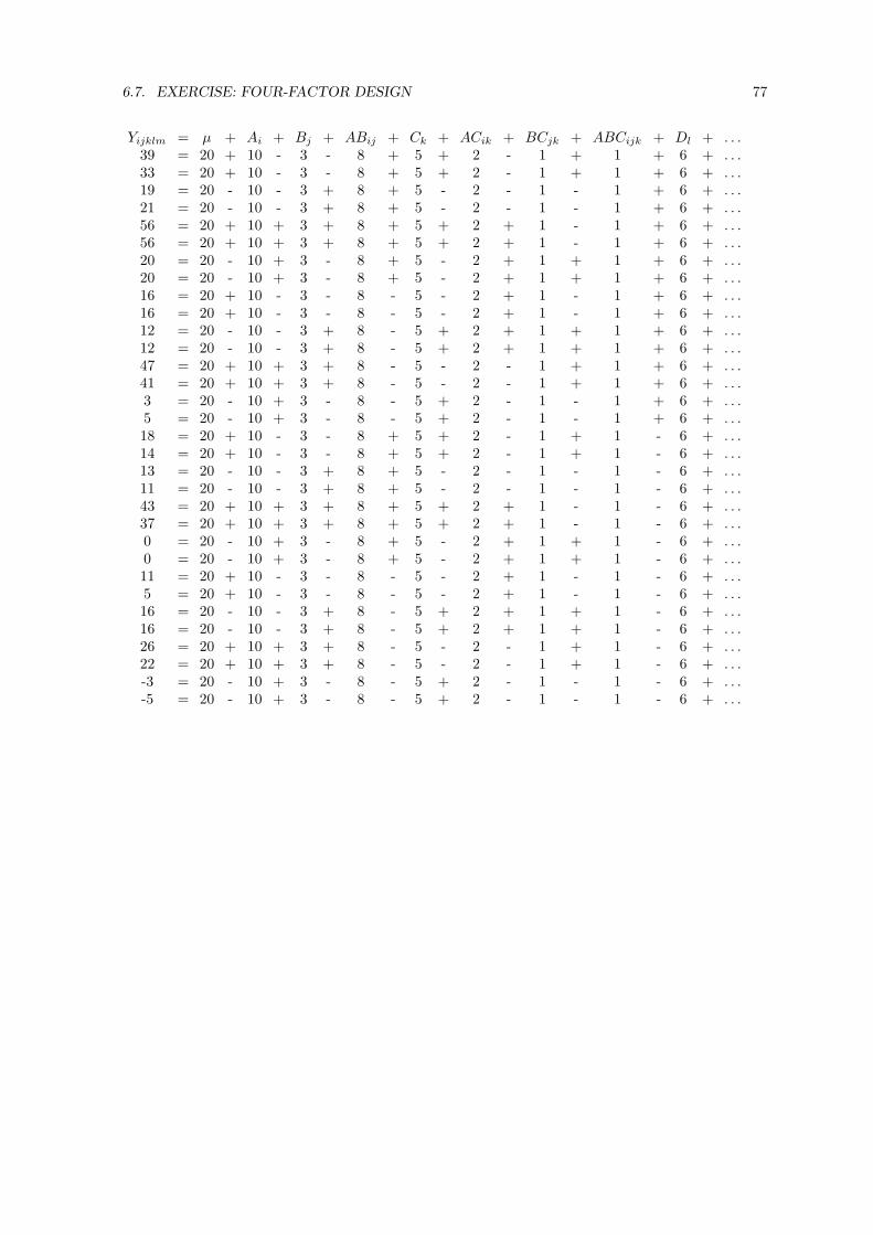
6.7. EXERCISE: FOUR-FACTOR DESIGN 77
Yijklm = µ + Ai + Bj + ABij + Ck + ACik + BCjk + ABCijk + Dl + . . .39 = 20 + 10 - 3 - 8 + 5 + 2 - 1 + 1 + 6 + . . .33 = 20 + 10 - 3 - 8 + 5 + 2 - 1 + 1 + 6 + . . .19 = 20 - 10 - 3 + 8 + 5 - 2 - 1 - 1 + 6 + . . .21 = 20 - 10 - 3 + 8 + 5 - 2 - 1 - 1 + 6 + . . .56 = 20 + 10 + 3 + 8 + 5 + 2 + 1 - 1 + 6 + . . .56 = 20 + 10 + 3 + 8 + 5 + 2 + 1 - 1 + 6 + . . .20 = 20 - 10 + 3 - 8 + 5 - 2 + 1 + 1 + 6 + . . .20 = 20 - 10 + 3 - 8 + 5 - 2 + 1 + 1 + 6 + . . .16 = 20 + 10 - 3 - 8 - 5 - 2 + 1 - 1 + 6 + . . .16 = 20 + 10 - 3 - 8 - 5 - 2 + 1 - 1 + 6 + . . .12 = 20 - 10 - 3 + 8 - 5 + 2 + 1 + 1 + 6 + . . .12 = 20 - 10 - 3 + 8 - 5 + 2 + 1 + 1 + 6 + . . .47 = 20 + 10 + 3 + 8 - 5 - 2 - 1 + 1 + 6 + . . .41 = 20 + 10 + 3 + 8 - 5 - 2 - 1 + 1 + 6 + . . .3 = 20 - 10 + 3 - 8 - 5 + 2 - 1 - 1 + 6 + . . .5 = 20 - 10 + 3 - 8 - 5 + 2 - 1 - 1 + 6 + . . .18 = 20 + 10 - 3 - 8 + 5 + 2 - 1 + 1 - 6 + . . .14 = 20 + 10 - 3 - 8 + 5 + 2 - 1 + 1 - 6 + . . .13 = 20 - 10 - 3 + 8 + 5 - 2 - 1 - 1 - 6 + . . .11 = 20 - 10 - 3 + 8 + 5 - 2 - 1 - 1 - 6 + . . .43 = 20 + 10 + 3 + 8 + 5 + 2 + 1 - 1 - 6 + . . .37 = 20 + 10 + 3 + 8 + 5 + 2 + 1 - 1 - 6 + . . .0 = 20 - 10 + 3 - 8 + 5 - 2 + 1 + 1 - 6 + . . .0 = 20 - 10 + 3 - 8 + 5 - 2 + 1 + 1 - 6 + . . .11 = 20 + 10 - 3 - 8 - 5 - 2 + 1 - 1 - 6 + . . .5 = 20 + 10 - 3 - 8 - 5 - 2 + 1 - 1 - 6 + . . .16 = 20 - 10 - 3 + 8 - 5 + 2 + 1 + 1 - 6 + . . .16 = 20 - 10 - 3 + 8 - 5 + 2 + 1 + 1 - 6 + . . .26 = 20 + 10 + 3 + 8 - 5 - 2 - 1 + 1 - 6 + . . .22 = 20 + 10 + 3 + 8 - 5 - 2 - 1 + 1 - 6 + . . .-3 = 20 - 10 + 3 - 8 - 5 + 2 - 1 - 1 - 6 + . . .-5 = 20 - 10 + 3 - 8 - 5 + 2 - 1 - 1 - 6 + . . .

78 CHAPTER 6. GENERALIZATION OF BETWEEN-SUBJECT DESIGNS
+ ADil + BDjl + ABDijl + CDkl + ACDikl + BCDjkl + ABCDijkl + S(ABCD)ijklm
+ 2 - 2 + 1 + 2 - 1 + 1 + 1 + 3+ 2 - 2 + 1 + 2 - 1 + 1 + 1 - 3- 2 - 2 - 1 + 2 + 1 + 1 - 1 - 1- 2 - 2 - 1 + 2 + 1 + 1 - 1 + 1+ 2 + 2 - 1 + 2 - 1 - 1 - 1 + 0+ 2 + 2 - 1 + 2 - 1 - 1 - 1 + 0- 2 + 2 + 1 + 2 + 1 - 1 + 1 + 0- 2 + 2 + 1 + 2 + 1 - 1 + 1 + 0+ 2 - 2 + 1 - 2 + 1 - 1 - 1 + 0+ 2 - 2 + 1 - 2 + 1 - 1 - 1 + 0- 2 - 2 - 1 - 2 - 1 - 1 + 1 + 0- 2 - 2 - 1 - 2 - 1 - 1 + 1 + 0+ 2 + 2 - 1 - 2 + 1 + 1 + 1 + 3+ 2 + 2 - 1 - 2 + 1 + 1 + 1 - 3- 2 + 2 + 1 - 2 - 1 + 1 - 1 - 1- 2 + 2 + 1 - 2 - 1 + 1 - 1 + 1- 2 + 2 - 1 - 2 + 1 - 1 - 1 + 2- 2 + 2 - 1 - 2 + 1 - 1 - 1 - 2+ 2 + 2 + 1 - 2 - 1 - 1 + 1 + 1+ 2 + 2 + 1 - 2 - 1 - 1 + 1 - 1- 2 - 2 + 1 - 2 + 1 + 1 + 1 + 3- 2 - 2 + 1 - 2 + 1 + 1 + 1 - 3+ 2 - 2 - 1 - 2 - 1 + 1 - 1 + 0+ 2 - 2 - 1 - 2 - 1 + 1 - 1 + 0- 2 + 2 - 1 + 2 - 1 + 1 + 1 + 3- 2 + 2 - 1 + 2 - 1 + 1 + 1 - 3+ 2 + 2 + 1 + 2 + 1 + 1 - 1 + 0+ 2 + 2 + 1 + 2 + 1 + 1 - 1 + 0- 2 - 2 + 1 + 2 - 1 - 1 - 1 + 2- 2 - 2 + 1 + 2 - 1 - 1 - 1 - 2+ 2 - 2 - 1 + 2 + 1 - 1 + 1 + 1+ 2 - 2 - 1 + 2 + 1 - 1 + 1 - 1
ANOVA:
Source df SS MS F Error Termµ 1 12800.0 12800.0 2133.333 S(ABCD)A 1 3200.0 3200.0 533.333 S(ABCD)B 1 288.0 288.0 48.000 S(ABCD)AB 1 2048.0 2048.0 341.333 S(ABCD)C 1 800.0 800.0 133.333 S(ABCD)AC 1 128.0 128.0 21.333 S(ABCD)BC 1 32.0 32.0 5.333 S(ABCD)ABC 1 32.0 32.0 5.333 S(ABCD)D 1 1152.0 1152.0 192.000 S(ABCD)AD 1 128.0 128.0 21.333 S(ABCD)BD 1 128.0 128.0 21.333 S(ABCD)ABD 1 32.0 32.0 5.333 S(ABCD)CD 1 128.0 128.0 21.333 S(ABCD)ACD 1 32.0 32.0 5.333 S(ABCD)BCD 1 32.0 32.0 5.333 S(ABCD)ABCD 1 32.0 32.0 5.333 S(ABCD)S(ABCD) 16 96.0 6.0Total 32 21088.0

Chapter 7
Within-Subjects Designs
7.1 Within- vs. Between-Subject Designs
All of the experimental designs we have considered so far have been fully between-subjects designs.In such designs each subject is tested in exactly one condition (i.e., at one level of the experimentalfactor or one combination of levels of the experimental factors). In essence, this means that eachsubject is tested in just one cell of the design. For example, in a one-way between-subjects design, ifa subject is tested at level 1 of the factor, he is never tested at level 2 or 3 or any other level (e.g.,in an experiment where college class was a factor, each subject would be tested as either a freshman,sophomore, junior, or senior, but not as more than one of these). In a two-way between-subjectsdesign, if a subject is tested in the condition defined by level 1 of Factor A and level 4 of Factor B(AB14, e.g., male senior), he is never tested in cell AB24 (female senior) or AB12 (male sophomore)and so on.
We will now begin considering a new class of experimental design, in which each subject is testedin every cell of the experiment. This type of design is called a within-subjects design.1 For example,in a one-factor within-subjects design exploring the effect of being in a particular college class, eachsubject would have to be measured four times: once as a freshman, again as a sophomore, again as ajunior, and finally as a senior. If drunk vs. sober were a second within-Ss factor in the design, eachsubject would have to be tested twice each year (once drunk and once sober), for a total of eight testsper subject. Obviously, not all factors can be tested within-subjects. For example, it is impossibleto test each subject at both levels of the gender factor. Similarly, you can’t compare two differentmethods for teaching French in a within-subjects design. Once you have taught subjects with onemethod, you can’t start over from the beginning and teach them with the other method.
Between-subjects designs can be very useful in many research situations, especially those in whichit is easy to test lots of subjects in each condition. Furthermore, they are the only option with factorslike gender. Nonetheless, many researchers prefer to use within-subjects designs whenever possible,because within-subjects designs are less influenced by random error than between-subjects designs.Within-subjects designs thus have greater power2 than between-subjects designs. In the remainderof this section we will explain why within-subjects designs are less affected by random variation. Insubsequent sections we will explain how to perform ANOVA on within-subjects designs. Finally, wewill present some example data sets and analyses.
Random error causes two types of problems in between-subjects designs. The first is that theaverage results can be severely influenced by accidental differences between groups of subjects testedin different conditions. Imagine for example that you are testing motor task performance underconditions of sleep loss vs. normal sleep. You test subjects’ motor performance by having them tryto throw a basketball through a basketball hoop. One group performs the task after a good night’ssleep; the other after staying awake for 24 hours. You randomly select 10 subjects and randomlyassign five to each group. Unfortunately, your random selection and assignment happens to place allfive starting members of the college basketball team in one group and five dedicated couch potatoes
1More formally, we have the following definitions: An experimental factor for which each subject is tested at everylevel is called a within-subjects factor. An experimental design composed entirely of within-subjects factors is called afully within-subjects design.
2In statistical terms, power is the probability of rejecting H0 when it is false—i.e., of detecting the error in the H0.Other things being equal (e.g., sample size), an experiment will have more power to the extent that the scores are lessinfluenced by random variability.
79

80 CHAPTER 7. WITHIN-SUBJECTS DESIGNS
in the other. (Granted, this is an unlikely occurrence, but with random selection and assignment, anygiven pattern is logically possible.)
If you happen to place the basketball players in the normal sleep condition and the couch potatoesin the sleep loss condition, your data will probably suggest that sleep loss adversely affects motorperformance much more than it really does. Worse yet, if you happen to place the basketball playersin the sleep loss condition and the couch potatoes in the rested condition, your data may well show thatthe sleep loss group performs significantly better than the rested group.3 Will you conclude that sleeploss enhances motor performance? Will this be the end of your career as a research scientist? Eitherway the groups are assigned, though, it is clear that an accidentally occurring difference between yourtwo groups of subjects greatly distorts the true effect of your experimental manipulation.
The second problem created by error in between-subjects designs can be seen when we consider thecharacter of the Fobserved. An F is essentially the ratio of effect size to error, where error is measuredas the differences between subjects in the same condition. A large Fobserved convinces us that the effectcould not have occurred due to chance, since our obtained within-cell error estimates the disparityof scores expected in this population due to chance. However, in a between-subjects design, we mayobtain a small Fobserved even when there exists a true effect of our experimental factor, simply becausethe effect is small relative to the random variation in the population.
To illustrate this second disadvantage, let us consider another farfetched example (we will see somerealistic examples later). You want to find out whether people weigh more with their clothes on thanwith their clothes off. You randomly select 10 people and weigh them fully dressed; you randomlyselect another 10 people and weigh them without clothes. The average person probably wears aboutfive pounds of clothes, so the mean of the dressed group should be about five pounds greater than themean of the not dressed group. However, the weight variation among a randomly selected group of 10people will be very large compared to that five pound difference. If you select from a population ofcollege undergraduates, your subjects’ weight may range from under 100 to over 250 pounds. Thus,the within-cell error term in your ANOVA will be very large relative to the main effect term, and youmay not obtain a significant main effect of the clothes on/off factor. Although increasing the samplesize could overcome this random variation (because the mean of a sample is known more precisely asthe sample size increases), the general point is still valid: With any given sample size, you have lesschance of rejecting a false H0 (i.e., less power) when random variation between subjects contributesto the error term.
Within-subjects designs solve both of the problems caused by random variation between subjects.In the basketball example, you could have each subject shoot baskets one day when fully rested andanother day when sleep deprived. There would then be no way that the people tested in the restedgroup could be inherently more or less skilled that the people tested in the sleep-deprived group,because they would be the very same people.
In the clothes on/off example, you could weigh a subject with his clothes on and then weigh thesame subject with his clothes off. Although there will still be variation in weight from one subject tothe next, this variation will not conceal the main effect of clothes because within-subjects designs allowus to compute an error term that is unaffected by this kind of random variation between subjects. Wewill explain how this is done below. Put very simply, the main effect of clothes will be clear becauseeach subject will show it (i.e., every subject will weigh more when dressed than when not).
In summary, the main advantages of the within-subjects design over the between-subjects designare that it eliminates effects of a priori group differences and provides a more sensitive measureof error than the simple within-cell variation used as the error term in between-subjects designs.4
Thus, within-subjects designs are preferred in many types of experiments, including tests of variousmedications, of teaching techniques, of manipulations expected to effect motor coordination, visualprocessing, reading ability, reflexes, etc. Essentially, a within-subjects design should be seriouslyconsidered any time the subjects differ greatly from one another in their overall scores on the DV.
There are certain practical problems associated with within-subjects factors, however. As we havealready seen, some manipulations simply do not lend themselves to this type of design. Gender andethnic group for example, must always be between-subjects factors; age can only be a within-subjectsfactor if subjects can be tested repeatedly over a period of some years. Second, use of within-subjectsfactors introduces order effects. That is, the results of an experiment may vary depending on the order
3In this example, the true impact of sleep loss on motor performance can clearly be masked by an a priori differencebetween the two groups of subjects. Probably, sleep loss does adversely affect motor performance, but, if the tiredbasketball team can outshoot the rested couch potatoes, you will not observe the true effect, and may observe itsopposite.
4Be careful of the somewhat confusing terminology: Between-subjects designs have within-cell error terms.

7.2. MODELS FOR WITHIN-SS DESIGNS 81
in which subjects are tested in the within-subjects conditions. For example, it can become impossibleto measure the effects of a second medication if the first medication given cures the condition; acomparison of techniques for teaching reading must consider the improvement in skill resulting fromCondition 1 when testing Condition 2; even our basketball example may be subject to order effects ifsubjects’ ability to shoot baskets was improved by the practice they received in the first condition. Itis possible to control for order effects when testing within-subjects factors, although this can be verytricky; we will discuss one approach after studying mixed designs (i.e., those having both between-and within-subjects factors).
7.2 Models for Within-Ss Designs
ANOVA is computed very similarly for within- and between-subjects designs, but there are twoimportant differences: 1) use of a within-subjects design introduces some new terms to the model,and 2) it complicates the selection of error terms for computing Fobserved values. In this section, weconsider how models are different in within-subjects designs. To illustrate these new terms, we willconsider a specific example of a within-subjects design.
Suppose that we are interested in studying problem solving by congressmen. We might randomlyselect six congressmen, give each one a series of logic problems, and measure the time they requiredto solve each one. Furthermore, suppose that we want to compare problem solving under differentconditions likely to be encountered in office. For example, we might want to compare problem solvingspeeds under four stress conditions: 1) normal working conditions, 2) after 2 glasses of wine, 3) afterbeing awakened in the middle of the night, and 4) in the midst of a bad head cold. The data mightlook like those in Table 7.1.
Decision-Making Condition:Congressman Normal Wine Awaken Cold AverageMr. Rockford 121 134 133 128 129Mr. Columbo 121 139 141 135 134Mrs. Fletcher 113 125 129 113 120Mr. Mason 123 139 137 129 132Mr. Chan 126 140 143 143 138Miss Marple 110 121 133 144 127Average 119 133 136 132 130
Table 7.1: Decision Making by Congressmen
The appropriate model for these data is:
Yij = µ + Ai + Sj + ASij
As always, we use Y to stand for the scores themselves. We need two subscripts to uniquely identifyeach of the scores. The subscript i indicates the level of the conditions factor and j indicates thecongressman (i.e., subject).
The within-subjects model still has the baseline (µ) and the main effect of conditions (Ai). Therationale is exactly as before: We expect each score to be influenced by the overall baseline level ofscoring and by the experimental manipulation.
The model also contains some new terms, peculiar to within-subjects designs. First, consider thenew Sj term. Recall that the function of the linear model is to divide up data values into componentsdue to various sources. For example, the function of a main effect term is to describe an overalldeviation from the baseline of a whole set of scores (e.g., all those obtained after two glasses of wine).These scores are expected to have a common overall deviation from the baseline because they are allobtained under conditions that are somehow similar. In earlier designs for example, we used maineffect terms to describe a common deviation from baseline due to scores coming from people of thesame gender. The idea was that people of the same gender have something in common, so their scoresmight have some common component as well.
What is new in a within-subjects design is that we have several scores from each subject. Multiplescores from the same person certainly have something in common, and the model represents thiscommonality by including the Sj term to take into account a main effect of subject. Just as the model

82 CHAPTER 7. WITHIN-SUBJECTS DESIGNS
has a term to reflect what is common about all the scores taken in a sleep-deprived condition, forexample, it has a term to reflect what is common to all of Congressman Rockford’s scores (or anyother subject). This subjects term has special importance in within-subject designs, so we will usethe letter S as the subject main effect term in all models, to distinguish it from experimental factorsA, B, C, etc.
In short, Sj reflects the effect of Subject j on a set of scores for that subject, just as Ai reflectsthe effect of Condition i on a set of scores for that condition. Naturally, we will use the data to getestimates, Sj , of the true values of Sj . What can we infer from the values of Sj that we estimate? As
we will see later, each Sj is calculated as the difference between the average score of Subject j and theaverage of all scores in the data set. Thus, it will be distant from zero to the extent that Subject j’sscores are different from the average of all scores from all subjects. In plainer language, if subjectsperform very differently from each other on the average across experimental conditions, the Sj values
will be large (positively and negatively); if subjects’ average performances are very similar, the Sj ’swill be small.
The model also has a term representing the interaction between the experimental factor, A, andthe subjects factor. This ASij interaction term is analogous to an ordinary interaction term: itmeasures the extent to which the effect of Factor A differs from subject to subject. For example,one congressman might solve problems more slowly in the middle of the night than after having twoglasses of wine, while another congressman might show the reverse pattern.
In between-subjects designs, we saw that interaction terms are large to the extent that the effectof one factor depends on the level of the other. Analogously, the ASij ’s are large to the extent thatthe effect of Factor A depends on which subject is being tested.
It is extremely important to understand that Sj and ASij provide information about two verydistinct kinds of differences among subjects. Sj indicates how Subject j differs from the other subjectswith respect to overall level of performance—i.e., performance on average across the conditions tested.For example, we might test one congressman who is methodical and thorough by nature and anothercongressman who is quicker and more impetuous. The methodical congressman would tend to takemore time to solve problems in all conditions of the experiment, which would produce a positive Sj
for him, since the DV is decision time. The quicker congressman would tend to solve problems morerapidly in all conditions of the experiment, which would make his Sj negative. Therefore, Sj measuresindividual differences that affect a person’s performance in the same direction in all conditions of theexperiment.
ASij measures a very different sort of variation among individuals: variation in how they respondto the different conditions of the experiment. To illustrate that this is indeed a different sort ofvariation, we will discuss two pairs of congressman.
First, consider again the thorough and impetuous congressmen discussed above. Whereas theyare very different in overall level of performance, they might respond exactly the same way to theexperimental manipulation. For example, both might take exactly 5 minutes more to solve a problemin the middle of the night than during the day. Thus, we see that it is possible for two subjects tohave very different values of Sj and yet have very similar values of ASij .
Second, consider two equally thorough congressmen, with identical large values of Sj . But supposeone is a very light sleeper and the other very sound sleeper. The light sleeper might solve problemsalmost as fast in the middle of the night as during the day, whereas the sound sleeper might workmuch more slowly in the middle of the night than during the day. If so, we might obtain a muchbigger effect of condition of testing for the sound sleeper than for the light sleeper. Thus, we see thatit is also possible for two subjects to have very similar values of Sj and yet have very different valuesof ASij for a given condition.
In summary, Sj measures overall variation from subject to subject. ASij , on the other hand,measures condition-specific variation from subject to subject. Alternatively, one can also say thatASij measures how much the experimental effect varies from subject to subject.
To better understand the difference between Sj and ASij , it is useful to compare the four datasets in Table 7.2. The data from each set are plotted in Figure 7.1, using a format similar to that ofa factorial plot.5
5Strictly speaking, these are not true factorial plots, because individual subject data rather than mean values areplotted. Note the similarity to a factorial plot, though: Levels of one factor (A) are arranged on the horizontal axis,and levels of another factor (S) are indicated by different lines on the plot.

7.2. MODELS FOR WITHIN-SS DESIGNS 83
A: Small values of S and ASDecision-Making Condition:
Congressman Normal Wine Awaken Cold AverageMr. Rockford 123 136 141 132 133Mr. Columbo 120 134 137 125 129Mrs. Fletcher 121 135 137 131 131Mr. Mason 123 137 137 131 132Mr. Chan 121 137 140 130 132Miss Marple 106 119 124 143 123Average 119 133 136 132 130
B: Large S and small ASDecision-Making Condition:
Congressman Normal Wine Awaken Cold AverageMr. Rockford 118 132 135 127 128Mr. Columbo 123 138 140 135 134Mrs. Fletcher 101 115 118 110 111Mr. Mason 130 143 147 140 140Mr. Chan 140 154 157 149 150Miss Marple 102 116 119 131 117Average 119 133 136 132 130
C: Small S and large ASDecision-Making Condition:
Congressman Normal Wine Awaken Cold AverageMr. Rockford 133 126 134 127 130Mr. Columbo 130 134 152 112 132Mrs. Fletcher 119 134 145 126 131Mr. Mason 107 123 143 147 130Mr. Chan 109 137 151 127 131Miss Marple 116 144 91 153 126Average 119 133 136 132 130
D: Large values of S and ASDecision-Making Condition:
Congressman Normal Wine Awaken Cold AverageMr. Rockford 136 129 137 130 133Mr. Columbo 139 143 161 121 141Mrs. Fletcher 137 152 163 144 149Mr. Mason 99 115 135 139 122Mr. Chan 98 126 140 116 120Miss Marple 105 133 80 142 115Average 119 133 136 132 130
Table 7.2: Sample Data Sets Illustrating S and AS
In Data Set A, both S and AS have small effects. The overall level of performance does not varygreatly from one subject to the next, nor does the pattern of condition effects vary much from subjectto subject. In the graph, this is apparent from the fact that the lines for the different subjects are allvery similar.
In Data Set B, S has a large effect but AS has a small one. The former can be seen from the factthat the overall level of performance varies greatly from one subject to another. For example, Mrs.Fletcher’s scores are in the low 100’s, but Mr. Chan’s scores are around 150. Thus there is a largedifference between subjects, and we would expect the Sj terms for this data set to be very differentfrom zero.
Note also that the pattern of effect caused by the experimental factor is almost identical for

84 CHAPTER 7. WITHIN-SUBJECTS DESIGNS
Normal Wine Awaken Cold
80
100
120
140
160
Dec
isio
nS
peed
AMarpleRockfordFletcherMasonChanColumbo
Normal Wine Awaken Cold
80
100
120
140
160 BChanMasonColomboMarpleRockford
Fletcher
Normal Wine Awaken ColdCondition
80
100
120
140
160
Dec
isio
nS
peed
CMarpleMason
ChanFletcherRockfordColumbo
Normal Wine Awaken ColdCondition
80
100
120
140
160 DFletcherMarpleMasonRockfordColumboChan
Figure 7.1: Decision time as a function of condition and congressman.
all subjects in Data Set B. Since every subject shows nearly the same pattern across the fourconditions, the AS interaction is small. On average, scores are 11 points lower than baseline in theNormal condition, and 3, 6, and 2 points above baseline for the other three conditions, respectively.More importantly, every subject shows about this same pattern (note the nearly parallel lines inFigure 7.1B). Thus the effect of the experimental factor does not seem to depend on which subjectis being tested. Whenever an experimental effect is very consistent from subject to subject, the ASij
terms will be close to zero.Data Set C shows what happens when S is small but AS is large. The subjects have about the same
averages across the different conditions of the experiment—in other words, there is little differencebetween subjects in overall performance. But different subjects show very different patterns of effectsacross the experimental conditions, as reflected in the decidedly nonparallel lines of Figure 7.1C. Forexample, most subjects score highest in the Awaken condition, but Miss Marple gets her lowest scoreby far in this condition.
Data Set D shows what happens with relatively large values for both S and AS. Here, the subjectsvary quite a bit in overall level, and also show very different patterns of effects across the fourconditions.
To summarize this set of four examples, Sj and ASij reflect two different types of variation fromsubject to subject: overall level vs. pattern of effect. These two types of variation are separate fromone another, as demonstrated by the fact that it is possible to construct data sets in which they areindependently large or small.
It is also instructive to consider why we have the ASij interaction term in the model for a within-subjects design but we do not have it in the model for a between-subjects design. By definition, awithin-subjects design gives us a score for each subject at each level of the experimental factor. Thus,we can measure the effect of Factor A separately for each individual subject. For example, look at anysingle line in Figure 7.1. The effect of A, for the subject represented by that line, is measured by howmuch the line deviates from a straight, horizontal line. Because we can measure the effect of A foreach subject, we can see how much it varies from subject to subject, and this is what ASij measures.
In contrast, between-subjects designs do not allow us to measure the effect of an experimental

7.2. MODELS FOR WITHIN-SS DESIGNS 85
factor for each subject. Each subject is observed at only one level of the factor, so we can onlyevaluate the effect of the factor by comparing groups of subjects, not by looking at the data from anyindividual subject.
We can easily extend this treatment of within-subjects models to a design having two within-subjects factors, A and B. In such a design, each subject would have to be tested at all combinationsof levels on Factors A and B. Assuming that each experimental factor has two levels, the data wouldhave the structure shown in Table 7.3.
ConditionSubject AB11 AB12 AB21 AB22
1 443 467 453 4372 363 387 373 3573 353 377 363 3474 402 426 416 3965 404 428 410 398
Average 393 417 403 387
Table 7.3: Sample Data for a Two-Factor, Within-Ss Design
The linear model for this design is:
Yijk = µ + Ai + Bj + ABij + Sk + ASik + BSjk + ABSijk
As before, the model contains a baseline, plus main effect and interaction terms for the experimentalfactors (A, B, AB). We again have a main effect term for subjects, so the model can take into accountwhat is common to all scores from a given subject.
We also have terms for the two-way interactions AS and BS. The former measures the extentto which the effect of Factor A varies from subject to subject, and the latter measures the extent towhich the effect of Factor B varies from subject to subject. Both of these terms can be understood injust the same way as the AS term in the model for the one-factor within-subjects design above (i.e.,Congressmen experiment). The only complication is that now we have to do a little averaging to seeeach main effect on a given subject. For example, to see the main effect of Factor A on Subject 1, wehave to compare the average of the scores at A1 (443 and 467) against the average of the scores at A2
(453 and 437).The entirely new term is ABSijk, which represents the three-way interaction between Factors A,
B, and S. This term is analogous to a three-way interaction term in a fully between-subjects design:it measures the extent to which the ABij interaction term depends on the level of subject (i.e., variesfrom subject to subject). Again, the major idea is that we have measured this interaction for eachsubject separately (note that we could plot the AB interaction for subject 1, for subject 2, etc.), sowe can see how much the interaction varies from subject to subject.
In summary, constructing the model for a within-subjects design is very similar to constructinga model for a between-subjects design. Models for within-subjects designs contain all the terms forexperimental factors and their interactions that are found in between-subjects models. Instead of asingle error term, though, within-subjects models contain a main effect term for subjects (always calledS), and terms for the interaction of subjects with each main effect and interaction of experimentalfactors.
The rationale behind the introduction of the subjects factor can be summarized as follows: Thelinear model is used to describe scores in terms of their common components. When we perform anexperiment using a within-subjects design, we obtain more than one score from each subject. Thesescores have something in common by virtue of the fact that they all came from the same individual,so the linear model must have a term that represents this common influence.
The rationale for the terms representing the interaction of subjects with experimental factors canbe summarized like this: Because we have measured each experimental effect on every subject, we canmeasure how much it varies from one subject to the next. Because we have measured each interactionof experimental factors on every subject, we can also measure how much the interaction varies fromsubject to subject.

86 CHAPTER 7. WITHIN-SUBJECTS DESIGNS
Finally, we can state the general rules needed to construct the linear model for any within-subjectsdesign.
• Y has one subscript for each experimental factor, and one for subjects.
• Include µ, main effects and interactions of all experimental factors.
• Include an S main effect.
• Include an interaction of S with all main effects and interactions of experimental factors. Thatis, include:
– All two-way interactions of an experimental factor and S.
– All three-way interactions of two experimental factors and S.
– All four-way interactions of three experimental factors and S.
– And so on, up to the interaction of all experimental factors and S.
7.3 Estimation and Decomposition
Once we have the correct model for a within-subjects design, no new ideas or procedures are neededto estimate the values of model terms or to compute SS’s and df’s. The value of a term is estimatedby taking the relevant data average and subtracting off whatever is explainable by simpler terms inthe model. This process can be repeated as often as necessary to construct a decomposition matrix.As always, the sum of squares for a term can be found by squaring and totalling the numbers in thecorresponding column of the decomposition matrix.
Degrees of freedom are found in the usual way for all experimental factors and their interactions.The df for subjects is still the number of subjects minus the number of groups, but in this type ofdesign there is only one group. When there are no between-Ss factors, all of the subjects are logicallyequivalent.
We will now illustrate these general rules with a computational example, to demonstrate preciselyhow to perform the calculations. In this example we will proceed only as far as the computation ofmean squares. The correct computation of Fobserved is discussed in detail in Section 7.5.
Our first example data are given in Table 7.4. These data are a hypothetical comparison of people’sspeed of response to the onset of differently colored lights (blue, green and red). Each subject sat infront of a computer monitor and pressed a button as soon as any light appeared. The DV is the timefrom the onset of the light to the key press response, measured in milliseconds (one-thousandths of asecond). Each subject was tested once with each light.
Subject Blue Green Red Average1 405 399 423 4092 405 402 426 4113 407 401 428 4124 403 398 423 408
Average 405 400 425 410
Table 7.4: Sample Data for Calculations In One-Factor Within-Ss Design
We begin as always by constructing the linear model for the experimental design. As discussedabove, the linear model for a one-factor within-subjects design is:
Yij = µ + Ai + Sj + ASij
Next we compute estimates for each term in the model. This is done exactly as though theS term in our model was B. That is, the estimation process is identical to that for a two-way fullybetween-subjects design. Thus, µ is estimated as:
µ = Y.. = 410

7.3. ESTIMATION AND DECOMPOSITION 87
Ai is estimated by the average of all scores at level i of Factor A, minus µ:
Ai = Yi. − µ
A1 = 405 − 410 = −5
A2 = 400 − 410 = −10
A3 = 425 − 410 = 15
To estimate the subject terms, recall that Sj is computationally just another factor in the model.
Thus, analogous to the computations just performed for A, Sj is the average of all scores from subjectj, minus µ.
Si = Y.j − µ
S1 = 409 − 410 = −1
S2 = 411 − 410 = 1
S3 = 412 − 410 = 2
S4 = 408 − 410 = −2
The estimation equation for ASij is exactly what it would be for an ABij interaction term, withS replacing B throughout.
ASij = Yij − µ − Ai − Sj
AS11 = 405 − 410 − (−5) − (−1) = 1
...
Using this equation for each pair of i and j values, we obtain the following table of ASij values.
A1 A2 A3S1: 1 0 -1S2: -1 1 0S3: 0 -1 1S4: 0 0 0
Having estimated all the terms in the model, we can easily construct the decomposition matrixfor this analysis—just set each score equal to the sum of its estimated components, as always. Thematrix for this data set is shown in Table 7.5.
Given the decomposition matrix, the SS for each source is computed by squaring and totallingall scores in each column of the matrix. The MS for a term is equal to its SS divided by its df, asalways. So, we have done enough so far to calculate the results shown in the following partial ANOVAtable (note that no F’s are included—this requires discussion of error terms).
Source df SS MS F Error Termµ 1 2,017,200 2,017,200A 2 1,400 700S 3 30 10AS 6 6 1Total 12 2,018,636
For each source, df is calculated using the rules given above. The dfS equals three: four subjectsminus one group. The dfAS equals dfA × dfS = 6.
This computational example shows that estimation and decomposition proceed in just the same wayusing a within-subjects model as they do using between-subjects models. Additional computationalexamples, including some with more factors, are given in Section 7.7.

88 CHAPTER 7. WITHIN-SUBJECTS DESIGNS
Yij = µ + Ai + Sj + ASij
405 = 410 - 5 - 1 + 1399 = 410 - 10 - 1 + 0423 = 410 + 15 - 1 - 1405 = 410 - 5 + 1 - 1402 = 410 - 10 + 1 + 1426 = 410 + 15 + 1 + 0407 = 410 - 5 + 2 + 0401 = 410 - 10 + 2 - 1428 = 410 + 15 + 2 + 1403 = 410 - 5 - 2 + 0398 = 410 - 10 - 2 + 0423 = 410 + 15 - 2 + 0
Table 7.5: Decomposition Matrix for Colored Light Data
7.4 “Random-Effects” vs. “Fixed-Effects” Factors
Before we begin our discussion of how to compute Fobserved values in within-subjects designs, we mustconsider an important conceptual difference between the subjects factor and the other experimentalfactors. In most experiments we want to do more than simply draw conclusions specific to theparticular subjects we tested. We generally think of our subjects as representative of some largepopulation of subjects, and we want to draw conclusions that apply to the whole population. Becausewe want to generalize our conclusions to the whole population, we randomly select subjects from thatpopulation for testing in our experiment, and we hope that the randomly selected subjects will berepresentative of the whole population. Because we randomly select the levels of our subjects factorit is called a random factor or random effects factor.
In the formal language of ANOVA, we say that a factor is a random factor when it satisfies twocriteria. A factor is a random factor if and only if both of the following conditions apply:
Random Selection: The levels of the factor actually included in the experiment were chosen randomlyfrom a larger population of potential levels.
Generalized Conclusions: Conclusions are intended to apply to the whole population of potentiallevels of the random factor, not just the ones actually included in the experiment.
If a factor fails to meet either or both of these criteria, it is called a “fixed effects” or “fixed” factorin the design.
All of the factors we have considered other than the subjects factor were fixed effects factorsbecause we intentionally chose exactly which levels to test. In fact, it is almost always the case thatthe interesting experimental factors are fixed effects factors, since it is rare that we are interested indifferences among conditions that we have sampled randomly. However, the subjects factor is almostalways a random effects factor, since we generally select subjects randomly from a population andthen try to generalize the results to everyone in that population.
Suppose, for example, that we wanted to compare problem solving by congressmen under variousconditions, as discussed above. If we had three particular congressmen that we were interested incomparing (say we were trying to decide which of three candidates for a particular office to votefor), then subjects would be a fixed effects factor. Alternatively, we might be interested in drawinggeneral conclusions about problem solving speed under various conditions, and we would want thoseconclusions to apply to all congressmen. In this case we would not be interested in any individualcongressmen except as representatives of the whole population of congressmen. We would randomlyselect our subjects, and the subjects factor would then be a random effects factor.
If we were actually interested in generalizing our conclusions to all congressmen, we would surelywant to test a large sample of them (say 30) in all the conditions of the experiment, rather thantesting only a few congressmen as described above. Testing more congressmen would give us a betterchance of having a representative sample, and so would be more likely to lead to accurate conclusions.Note, however, that the number of congressmen tested makes little difference to the structure of thelinear model. With 30 subjects instead of 6, we would have the identical model, except the subscripton the subjects term (Sj) would range from 1 to 30 instead of 1 to 6. Testing more congressmen does

7.5. CHOICE OF ERROR TERM & COMPUTATION OF FOBSERV ED 89
not change the structure of the experimental design in any way, it merely adds levels to an alreadyexisting factor.
7.5 Choice of Error Term & Computation of Fobserved
7.5.1 Error as a “Yardstick”
In between-subjects designs, the Fobserved for any term is computed as:
FTerm =MSTerm
MSS(ABC...)
Intuitively, the MSS(ABC...) estimates the size of observed effects that one would expect to get entirelyby chance—with these subjects, under these conditions. The MSTerm measures the difference betweengroups of subjects in different conditions. If the FTerm is large, then the difference between groups waslarger than one would expect to get by chance, and we conclude that the observed difference reflectsa real population effect. The important idea is that MSS(ABC...) functions as an “error yardstick,”against which we measure the observed factor effects.
In a between-subjects design, the MS for subjects is our only measure of random variabilitybetween subjects, and is thus the only candidate for the role of yardstick. In within-subjects designshowever, we have several measures of subject variability. For example, we have seen that in a one-factor design, Sj measures overall subject variability, while ASij measures the extent to which theeffect of Factor A varies depending on the subject being tested. Both of these sources in some sensereflect sampling error (i.e., how much variability we would expect to find in our data due to chance),yet they represent different sources of that variability. Which MS should serve as the denominatorfor the Fobserved?
The answer is that different MS’s are used to compute F’s for different sources. To choose thecorrect error MS for each F, we must consider carefully which error measure provides the appropriateyardstick for each experimental effect or interaction.
7.5.2 Error Term for µ
We begin by finding the appropriate yardstick for testing H0: µ = 0. µ provides an estimate of theoverall population mean; thus, our confidence that the population mean differs from zero dependsboth on the size of µ and on the amount of variability in our data set. If µ is very large (positively ornegatively), we are more confident that the population mean is in fact non-zero than if µ is very small.However, to the extent that the scores in our data set are wildly variable (some positive and somenegative), we will have our doubts even about a very large µ. That is, a small µ in a very homogenousdata set may reflect a non-zero population mean while a larger µ from a very heterogenous data setmay not.
But which type of variability is relevant, that reflected in Sj or that reflected in ASij? The answeris Sj . To see why, compare Data Sets B and C in Table 7.2. In both cases, the overall average isµ = 130. In which case, though, are you more sure that the true µ is close to 130, say between 128and 132?
Consider Data Set B. If we were to randomly sample two new subjects, we could reasonably expectto get new subjects whose averages were anywhere in the range of about 110 to 150, because we havealready gotten subject averages in that range (see “average” column at far right of table). It is prettyeasy to imagine getting two new subjects with means in the 140 to 150 range, which would raise thegroup average well above 130. In other words, because of the high variability in the subject averagecolumn, the overall experiment average of 130 does not seem like a very stable number.
Now consider Data Set C. Here, if we were to sample two new subjects, we would expect theiraverages to fall in approximately the range of 125-135. There is little variability in the averages of thesubjects we have already observed, and so we would be surprised to see a new subject who was reallydiscrepant from the overall average of 130. Thus, because of the low variability in the subject averagecolumn, the overall experiment average of 130 seems more stable than the average in Data Set B.
What this comparison shows is that S variability is a good yardstick for uncertainty about µ.When S variability is high (Data Set B but not C), we have relatively more uncertainty about µ.When AS variability is high (Data Set C but not B), though, it does not increase uncertainty aboutµ. That is why we use S variability (i.e., MSS) rather than AS variability (i.e., MSAS) as the erroryardstick to test a hypothesis about µ.

90 CHAPTER 7. WITHIN-SUBJECTS DESIGNS
In summary, when we are interested in whether the overall mean might be different from zeroby chance, the relevant yardstick is the variability from subject to subject in overall score, and thisvariability is indexed by the Sj term. If the subjects are comparatively similar to one another inoverall level, then the average score observed in the experiment is probably pretty close to the trueaverage. If subjects vary wildly in overall level, then the average score observed in the experimentmay not be so close to the true average. Thus,
Fµ =MSµ
MSS
measures the ratio of the size of µ to the amount of variability in the subject averages.
7.5.3 Error Term for a Main Effect
Let us now consider how to compute Fobserved for a main effect. If we observe a large differencebetween various levels of an experimental factor, we are more likely to believe that the effect actuallyexists in the population than if we observe a very small difference. However, just as in all previouscalculations of Fobserved, we need a comparison value reflecting how much of an observed differencemight arise by chance.
The key insight is that any given observed difference is likely to be real (i.e., unlikely to have arisenby chance) if each of the subjects showed approximately the same effect. On the other hand, a givendifference is less likely to be real (i.e., more likely to have arisen by chance) if each of the subjectsshowed a rather different effect. In other words, the effect is probably real if it is consistent acrosssubjects, but it is probably just chance if it is very inconsistent across subjects.
To develop your understanding of this point, examine the data sets plotted in Figure 7.1. Theeffect of decision-making condition is the same, on average, in all four data sets, as is apparent from theidentical marginal averages for Condition in Table 7.2. But the data sets are not equally convincingthat this effect is representative of the whole population from which these subjects were sampled. InData Set A, the effect certainly appears real. The results are very consistent across subjects, and sowe can expect that we would get pretty much the same results if we sampled some other subjects.
Now consider Data Set B. These subjects are pretty different from one another in overall level (i.e.,separation between lines in the figure, caused by large values of Sj), but they all show pretty similareffects of decision-making condition (i.e., nearly parallel lines in the figure, caused by small valuesof ASij). If we take some new subjects from this population, we would certainly expect substantialvariation in the overall level of the subjects’ performance, as discussed in the previous section. Butwe would not expect much variation in the effect of decision-making condition; this effect is veryconsistent across these subjects, and so we would expect it to be consistent across other subjects fromthis population as well. Obviously the effect is more likely to be real if it is there for all subjects.This means that either of the two data sets, A or B, would be pretty good evidence that the effect ofdecision-making seen in the averages is representative of the whole population, precisely because thesize of the effect is consistent across subjects. Not coincidentally, the ASij terms are small in both ofthese data sets.
In contrast, Data Sets C and D show relatively unconvincing evidence for an effect of decision-making condition, even though the effect on average is the same size as in Data Sets A and B. Thereason is apparent in the plots: the effect of decision-making is very inconsistent across subjects ineach case. Looking at either of these plots, it is easy to imagine taking some new subjects with effectsquite different from those shown in the means, and so we can have relatively little confidence that themeans of the data set are representative of the population as a whole.
To sum up: To see whether a main effect is real or due to chance, we need an error yardstick thatmeasures how much the effect varies from subject to subject. Low variation suggests a real effect,whereas high variation suggests a chance effect.
In within-subjects designs, we have exactly the yardstick we require: the MSAS interaction term.By definition, this measures the extent to which the effect of Factor A varies from subject to subject.A large MSAS means that the effect of Factor A varies considerably from subject to subject, whereasa small MSAS means that Factor A has a very consistent effect. Thus, we compute the F for a maineffect as:
FA =MSA
MSAS

7.5. CHOICE OF ERROR TERM & COMPUTATION OF FOBSERV ED 91
7.5.4 Error Terms for Interactions
The above discussion can be easily extended to higher-order terms in within-subjects models. Forexample, suppose we want to determine whether an observed AB interaction is real or due to chance.We will tend to believe the interaction is real if it is consistent—that is, if every subject shows thesame pattern of interaction, or nearly so. Thus, we want to compare the observed AB interactionagainst a term which measures how much the AB interaction varies from subject to subject. But thatvariation is exactly what the ABS interaction term measures. Thus the FAB is:
FAB =MSAB
MSABS
Again, the rationale is exactly like that for the main effect: If the interaction is consistent from subjectto subject we can conclude that it is real, but if it is inconsistent (highly variable) we have more reasonto think that the pattern in the AB cell averages was observed by chance.
You can make the same argument for an interaction of any complexity you care to consider. Isan observed ABCD interaction real or due to chance? Well, is it consistent across subjects (lowMSABCDS) or not?
7.5.5 Error Term Summary
The concept of consistency underlies the rules for choosing a correct error yardstick—formally knownas “error term”—in within-subjects designs.
• To test H0: µ= 0, compute Fµ =MSµMSS
.
• To test H0: No effect of a factor, compute Ffactor =MSfactor
MSfactor by S interaction.
• To test H0: No interaction of factors ABC..., compute FABC... = MSABC...MSABC...S
.
Note that we do not normally compute F’s for the effect of subjects or interactions involvingsubjects. One reason is that it is not regarded as meaningful to test the hypothesis that somerandomly selected subjects are different from one another, or that randomly selected subjects showdifferent effects of an experimental manipulation. Generally, this is assumed, or known from previousresearch. If subjects were not different from one another, why would we bother to sample more thanone?
Occasionally, it is desirable to test the H0’s that the particular subjects in an experiment are allthe same in overall level, all have the same effect of Factor A, all show the same AB interaction, etc.The most appropriate way to do this is to treat Subjects as a fixed-effects factor and use an analysis fora between-subjects design. For this analysis, you are not regarding the individuals tested as randomlyselected subjects, but rather as a fixed sample. In fact, for this analysis the random “subject” reallycorresponds to separate tests of a given individual. This analysis requires more than one observationper subject in each condition. Then, you can do a between-subjects analysis treating subjects as aregular experimental factor, and you will get the appropriate F’s for testing the hypotheses aboutsubjects. Note that in this analysis the F’s for the other factors test whether or not there are effectsfor these subjects. It would be inappropriate to generalize significant effects on these subjects to thewhole population, because this analysis uses the wrong error term.
7.5.6 Comparison with Between-Subjects Designs
Now that you understand where error terms come from in within-subjects designs, you are in a goodposition to understand the old experimentalist’s rubric that within-subjects designs have more powerthan between-subjects designs. This is an important concept in experimental design, so it is worth abrief diversion from ANOVA computations.
The major flaw of between-subjects designs is that they do not provide an estimate of how theeffect of an experimental factor varies from subject to subject. Each subject is tested in only onecondition, so we cannot see how an individual subject’s score changes across conditions. That is, wecannot measure the effect of conditions for any single subject, so obviously we cannot see how thateffect varies from one subject to the next. More or less by default, these designs force us to usewithin-cell error as our yardstick, simply because there is no alternative.

92 CHAPTER 7. WITHIN-SUBJECTS DESIGNS
Consider what this within-cell error really is, however, in terms of the concepts of within-subjectsdesigns. In a between-subjects design, two subjects in the same cell may differ from one anothereither because they are different in overall level or because they respond differently to that level ofthe factor. That is,
S(A)ij = Sj + ASij
where the left side of the equation shows the between-subjects error term and the right side showsthe corresponding sum of within-subjects terms.
We now see why within-subjects designs tend to have smaller error terms (and thus be morepowerful) than between-subjects designs. In a within-subjects design we can essentially reduce ourerror by separating out random variability in overall subject scores from random variability in thesize of each subject’s main effect. If the main effect is consistent across subjects, then the error termwill be small even if subjects vary widely in overall level. Between-subjects designs are forced to lumpboth sources of error together, which may obscure a true population effect. For example, consider theexperiment to see whether people weigh more with their clothes on or off, discussed in Section 7.1.In the within-subjects design, only variation in the weight of the clothes enters into the error term,not variation in overall weight of the subject. In the between-subjects version both types of variationenter into the error term, which is thereby much larger. We will discuss this concept in more detailbelow when we look at some data sets and see the actual computations.
7.6 Interpretation of F’s
The interpretation of results in within-subjects designs is no different from that in between-subjectsdesigns. Significant main effects and interactions should be described and graphed. The fact thatthe factors were tested within-subjects rather than between-subjects generally has no influence on theinterpretation.6
7.7 Computational Examples
1. Design with one within-subjects factor. Subjects have to make a number of decisions in eachof three conditions varying in the type of pressure they are under. In a control condition, thereis no pressure. In a high-speed condition, there is time pressure (i.e., subjects have to decidequickly). In a high-importance condition, a lot depends on whether the subject gets the decisionright or not (e.g., big money bonuses for correct decisions, like on TV game shows). The DV isthe percentage of correct decisions in each condition.
Data:
Type of PressureNone Time Importance
Subject 1: 70 51 44Subject 2: 82 66 59Subject 3: 90 63 66Subject 4: 70 59 57Subject 5: 77 62 71Subject 6: 61 53 69
Model: Yij = µ + Ai + Sj + ASij
6There are some examples where effects are really larger in a within-subjects design than in a between-subjectsdesign, or vice versa. Such findings are not a statistical matter, however, but reflect on the particular area of researchin which they are obtained.

7.7. COMPUTATIONAL EXAMPLES 93
Estimation Equations:
µ = Y..
Ai = Yi. − µ
Si = Y.j − µ
ASij = Yij − µ − Ai − Sj
Decomposition Matrix:
Yij = µ + Ai + Sj + ASij
70 = 65 + 10 - 10 + 551 = 65 - 6 - 10 + 244 = 65 - 4 - 10 - 782 = 65 + 10 + 4 + 366 = 65 - 6 + 4 + 359 = 65 - 4 + 4 - 690 = 65 + 10 + 8 + 763 = 65 - 6 + 8 - 466 = 65 - 4 + 8 - 370 = 65 + 10 - 3 - 259 = 65 - 6 - 3 + 357 = 65 - 4 - 3 - 177 = 65 + 10 + 5 - 362 = 65 - 6 + 5 - 271 = 65 - 4 + 5 + 561 = 65 + 10 - 4 - 1053 = 65 - 6 - 4 - 269 = 65 - 4 - 4 + 12
ANOVA:
Source df SS MS F Error Termµ 1 76050.0 76050.0 551.09 SA 2 912.0 456.0 9.01 ASS 5 690.0 138.0AS 10 506.0 50.6Total 18 78158.0
2. Design with two within-subjects factors.
Design:
• Factor A: 2 levels, Within-subjects.
• Factor B: 2 levels, Within-subjects.
• 3 Subjects per group. (Factor S has 3 levels.)
Data:
B1 B2 SubjectA1 A2 A1 A2 Averages
Subject 1 38 28 44 34 36Subject 2 41 35 41 39 39Subject 3 32 42 62 44 45Averages 37 35 49 39 40
Model: Yijk = µ + Ai + Bj + ABij + Sk + ASik + BSjk + ABSijk

94 CHAPTER 7. WITHIN-SUBJECTS DESIGNS
Estimation Equations:
µ = Y...
Ai = Yi.. − µ
Bj = Y.j. − µ
ABij = Yij. − µ − Ai − Bj
Sk = Y..k − µ
ASik = Yi.k − µ − Ai − Sk
BSjk = Y.jk − µ − Bj − Sk
ABSijk = Yijk − µ − Ai − Bj − ABij − Sk − ASik − BSjk
Decomposition Matrix:
Yijk = µ + Ai + Bj + ABij + Sk + ASik + BSjk + ABSijk
38 = 40 + 3 - 4 - 2 - 4 + 2 + 1 + 228 = 40 - 3 - 4 + 2 - 4 - 2 + 1 - 244 = 40 + 3 + 4 + 2 - 4 + 2 - 1 - 234 = 40 - 3 + 4 - 2 - 4 - 2 - 1 + 241 = 40 + 3 - 4 - 2 - 1 - 1 + 3 + 335 = 40 - 3 - 4 + 2 - 1 + 1 + 3 - 341 = 40 + 3 + 4 + 2 - 1 - 1 - 3 - 339 = 40 - 3 + 4 - 2 - 1 + 1 - 3 + 332 = 40 + 3 - 4 - 2 + 5 - 1 - 4 - 542 = 40 - 3 - 4 + 2 + 5 + 1 - 4 + 562 = 40 + 3 + 4 + 2 + 5 - 1 + 4 + 544 = 40 - 3 + 4 - 2 + 5 + 1 + 4 - 5
ANOVA Table:
Source df SS MS F Error Termµ 1 19200.0 19200.0 228.571 SA 1 108.0 108.0 9.000 ASB 1 192.0 192.0 3.692 BSAB 1 48.0 48.0 0.632 ABSS 2 168.0 84.0AS 2 24.0 12.0BS 2 104.0 52.0ABS 2 152.0 76.0Total 12 19996.0
3. Another design with two within-subjects factors.
Design:
• Factor A: 2 levels, Within-subjects.
• Factor B: 3 levels, Within-subjects.
• 5 Subjects per group.

7.7. COMPUTATIONAL EXAMPLES 95
Data:
B1 B2 B3 SubjectA1 A2 A1 A2 A1 A2 Average
Subject 1 63 31 71 53 58 36 52Subject 2 74 40 75 53 55 51 58Subject 3 81 35 83 51 73 49 62Subject 4 79 39 87 59 65 49 63Subject 5 33 15 29 29 49 25 30Average 66 32 69 49 60 42 53
Model and Estimation Equations: Same as previous design.
Decomposition Matrix:
Yijk = µ + Ai + Bj + ABij + Sk + ASik + BSjk + ABSijk
63 = 53 + 12 - 4 + 5 - 1 + 0 - 1 - 131 = 53 - 12 - 4 - 5 - 1 + 0 - 1 + 171 = 53 + 12 + 6 - 2 - 1 + 0 + 4 - 153 = 53 - 12 + 6 + 2 - 1 + 0 + 4 + 158 = 53 + 12 - 2 - 3 - 1 + 0 - 3 + 236 = 53 - 12 - 2 + 3 - 1 + 0 - 3 - 274 = 53 + 12 - 4 + 5 + 5 - 2 + 3 + 240 = 53 - 12 - 4 - 5 + 5 + 2 + 3 - 275 = 53 + 12 + 6 - 2 + 5 - 2 + 0 + 353 = 53 - 12 + 6 + 2 + 5 + 2 + 0 - 355 = 53 + 12 - 2 - 3 + 5 - 2 - 3 - 551 = 53 - 12 - 2 + 3 + 5 + 2 - 3 + 581 = 53 + 12 - 4 + 5 + 9 + 5 + 0 + 135 = 53 - 12 - 4 - 5 + 9 - 5 + 0 - 183 = 53 + 12 + 6 - 2 + 9 + 5 - 1 + 151 = 53 - 12 + 6 + 2 + 9 - 5 - 1 - 173 = 53 + 12 - 2 - 3 + 9 + 5 + 1 - 249 = 53 - 12 - 2 + 3 + 9 - 5 + 1 + 279 = 53 + 12 - 4 + 5 + 10 + 2 + 0 + 139 = 53 - 12 - 4 - 5 + 10 - 2 + 0 - 187 = 53 + 12 + 6 - 2 + 10 + 2 + 4 + 259 = 53 - 12 + 6 + 2 + 10 - 2 + 4 - 265 = 53 + 12 - 2 - 3 + 10 + 2 - 4 - 349 = 53 - 12 - 2 + 3 + 10 - 2 - 4 + 333 = 53 + 12 - 4 + 5 - 23 - 5 - 2 - 315 = 53 - 12 - 4 - 5 - 23 + 5 - 2 + 329 = 53 + 12 + 6 - 2 - 23 - 5 - 7 - 529 = 53 - 12 + 6 + 2 - 23 + 5 - 7 + 549 = 53 + 12 - 2 - 3 - 23 - 5 + 9 + 825 = 53 - 12 - 2 + 3 - 23 + 5 + 9 - 8
ANOVA Table:
Source df SS MS F Error Termµ 1 84270.0 84270.0 76.332 SA 1 4320.0 4320.0 49.655 ASB 2 560.0 280.0 5.283 BSAB 2 380.0 190.0 4.691 ABSS 4 4416.0 1104.0AS 4 348.0 87.0BS 8 424.0 53.0ABS 8 324.0 40.5Total 30 95042.0

96 CHAPTER 7. WITHIN-SUBJECTS DESIGNS
4. Design with 3 Within-subjects Factors.
Design:
• Factor A: 2 levels, Within-subjects.
• Factor B: 3 levels, Within-subjects.
• Factor C: 3 levels, Within-subjects.
• 3 Subjects per group.
Data:
A1C1 C2 C3
Subject B1 B2 B3 B1 B2 B3 B1 B2 B31 54 51 33 50 45 49 22 27 382 48 47 34 48 49 47 27 30 393 75 70 56 70 65 63 74 66 46
A2C1 C2 C3
Subject B1 B2 B3 B1 B2 B3 B1 B2 B31 74 65 65 54 45 57 52 49 522 86 69 58 66 57 57 67 60 473 71 58 66 84 63 75 76 56 72
Model:
Yijkl = µ + Ai + Bj + ABij + Ck + ACik + BCjk + ABCijk
+ Sl + ASil + BSjl + ABSijl + CSkl + ACSikl + BCSjkl + ABCSijkl
Estimation Equations:
µ = Y....
Ai = Yi... − µ
Bj = Y.j.. − µ
ABij = Yij.. − µ − Ai − Bj
Ck = Y..k. − µ
ACik = Yi.k. − µ − Ai − Ck
BCjk = Y.jk. − µ − Bj − Ck
ABCijk = Yijk. − µ − Ai − Bj − ABij − Ck − ACik − BCjk
Sl = Y...l − µ
ASil = Yi..l − µ − Ai − Sl
BSjl = Y.j.l − µ − Bj − Sl
ABSijl = Yij.l − µ − Ai − Bj − ABij − Sl − ASil − BSjl
CSkl = Y..kl − µ − Ck − Sl
ACSikl = Yi.kl − µ − Ai − Ck − ACik − Sl − ASil − CSkl
BCSikl = Y.jkl − µ − Bj − Ck − BCjk − Sl − BSjl − CSkl
ABCSijkl = Yijkl − µ − Ai − Bj − ABij − Ck − ACik − BCjk − ABCijk
−Sl − ASil − BSjl − ABSijl − CSkl − ACSikl − BCSikl

7.7. COMPUTATIONAL EXAMPLES 97
Decomposition Matrix:
Yijk = µ + Ai + Bj + ABij + Ck + ACik + BCjk + ABCijk + . . .54 = 56 - 7 + 5 - 2 + 4 - 1 + 3 + 1 + . . .74 = 56 + 7 + 5 + 2 + 4 + 1 + 3 - 1 + . . .51 = 56 - 7 - 2 + 3 + 4 - 1 + 2 + 1 + . . .65 = 56 + 7 - 2 - 3 + 4 + 1 + 2 - 1 + . . .33 = 56 - 7 - 3 - 1 + 4 - 1 - 5 - 2 + . . .65 = 56 + 7 - 3 + 1 + 4 + 1 - 5 + 2 + . . .50 = 56 - 7 + 5 - 2 + 2 + 3 - 1 + 0 + . . .54 = 56 + 7 + 5 + 2 + 2 - 3 - 1 + 0 + . . .45 = 56 - 7 - 2 + 3 + 2 + 3 - 2 + 0 + . . .45 = 56 + 7 - 2 - 3 + 2 - 3 - 2 + 0 + . . .49 = 56 - 7 - 3 - 1 + 2 + 3 + 3 + 0 + . . .57 = 56 + 7 - 3 + 1 + 2 - 3 + 3 + 0 + . . .22 = 56 - 7 + 5 - 2 - 6 - 2 - 2 - 1 + . . .52 = 56 + 7 + 5 + 2 - 6 + 2 - 2 + 1 + . . .27 = 56 - 7 - 2 + 3 - 6 - 2 + 0 - 1 + . . .49 = 56 + 7 - 2 - 3 - 6 + 2 + 0 + 1 + . . .38 = 56 - 7 - 3 - 1 - 6 - 2 + 2 + 2 + . . .52 = 56 + 7 - 3 + 1 - 6 + 2 + 2 - 2 + . . .48 = 56 - 7 + 5 - 2 + 4 - 1 + 3 + 1 + . . .86 = 56 + 7 + 5 + 2 + 4 + 1 + 3 - 1 + . . .47 = 56 - 7 - 2 + 3 + 4 - 1 + 2 + 1 + . . .69 = 56 + 7 - 2 - 3 + 4 + 1 + 2 - 1 + . . .34 = 56 - 7 - 3 - 1 + 4 - 1 - 5 - 2 + . . .58 = 56 + 7 - 3 + 1 + 4 + 1 - 5 + 2 + . . .48 = 56 - 7 + 5 - 2 + 2 + 3 - 1 + 0 + . . .66 = 56 + 7 + 5 + 2 + 2 - 3 - 1 + 0 + . . .49 = 56 - 7 - 2 + 3 + 2 + 3 - 2 + 0 + . . .57 = 56 + 7 - 2 - 3 + 2 - 3 - 2 + 0 + . . .47 = 56 - 7 - 3 - 1 + 2 + 3 + 3 + 0 + . . .57 = 56 + 7 - 3 + 1 + 2 - 3 + 3 + 0 + . . .27 = 56 - 7 + 5 - 2 - 6 - 2 - 2 - 1 + . . .67 = 56 + 7 + 5 + 2 - 6 + 2 - 2 + 1 + . . .30 = 56 - 7 - 2 + 3 - 6 - 2 + 0 - 1 + . . .60 = 56 + 7 - 2 - 3 - 6 + 2 + 0 + 1 + . . .39 = 56 - 7 - 3 - 1 - 6 - 2 + 2 + 2 + . . .47 = 56 + 7 - 3 + 1 - 6 + 2 + 2 - 2 + . . .75 = 56 - 7 + 5 - 2 + 4 - 1 + 3 + 1 + . . .71 = 56 + 7 + 5 + 2 + 4 + 1 + 3 - 1 + . . .70 = 56 - 7 - 2 + 3 + 4 - 1 + 2 + 1 + . . .58 = 56 + 7 - 2 - 3 + 4 + 1 + 2 - 1 + . . .56 = 56 - 7 - 3 - 1 + 4 - 1 - 5 - 2 + . . .66 = 56 + 7 - 3 + 1 + 4 + 1 - 5 + 2 + . . .70 = 56 - 7 + 5 - 2 + 2 + 3 - 1 + 0 + . . .84 = 56 + 7 + 5 + 2 + 2 - 3 - 1 + 0 + . . .65 = 56 - 7 - 2 + 3 + 2 + 3 - 2 + 0 + . . .63 = 56 + 7 - 2 - 3 + 2 - 3 - 2 + 0 + . . .63 = 56 - 7 - 3 - 1 + 2 + 3 + 3 + 0 + . . .75 = 56 + 7 - 3 + 1 + 2 - 3 + 3 + 0 + . . .74 = 56 - 7 + 5 - 2 - 6 - 2 - 2 - 1 + . . .76 = 56 + 7 + 5 + 2 - 6 + 2 - 2 + 1 + . . .66 = 56 - 7 - 2 + 3 - 6 - 2 + 0 - 1 + . . .56 = 56 + 7 - 2 - 3 - 6 + 2 + 0 + 1 + . . .46 = 56 - 7 - 3 - 1 - 6 - 2 + 2 + 2 + . . .72 = 56 + 7 - 3 + 1 - 6 + 2 + 2 - 2 + . . .

98 CHAPTER 7. WITHIN-SUBJECTS DESIGNS
. . . + Sk + ASik + BSjk + ABSijk + CSk + ACSik + BCSjk + ABCSijk
. . . - 7 - 1 - 3 + 1 + 4 - 2 + 2 + 1
. . . - 7 + 1 - 3 - 1 + 4 + 2 + 2 - 1
. . . - 7 - 1 + 0 - 1 + 4 - 2 + 1 + 1
. . . - 7 + 1 + 0 + 1 + 4 + 2 + 1 - 1
. . . - 7 - 1 + 3 + 0 + 4 - 2 - 3 - 2
. . . - 7 + 1 + 3 + 0 + 4 + 2 - 3 + 2
. . . - 7 - 1 - 3 + 1 - 1 + 3 + 1 + 1
. . . - 7 + 1 - 3 - 1 - 1 - 3 + 1 - 1
. . . - 7 - 1 + 0 - 1 - 1 + 3 - 1 + 0
. . . - 7 + 1 + 0 + 1 - 1 - 3 - 1 + 0
. . . - 7 - 1 + 3 + 0 - 1 + 3 + 0 - 1
. . . - 7 + 1 + 3 + 0 - 1 - 3 + 0 + 1
. . . - 7 - 1 - 3 + 1 - 3 - 1 - 3 - 2
. . . - 7 + 1 - 3 - 1 - 3 + 1 - 3 + 2
. . . - 7 - 1 + 0 - 1 - 3 - 1 + 0 - 1
. . . - 7 + 1 + 0 + 1 - 3 + 1 + 0 + 1
. . . - 7 - 1 + 3 + 0 - 3 - 1 + 3 + 3
. . . - 7 + 1 + 3 + 0 - 3 + 1 + 3 - 3
. . . - 4 - 4 + 0 - 3 + 1 - 2 + 2 - 1
. . . - 4 + 4 + 0 + 3 + 1 + 2 + 2 + 1
. . . - 4 - 4 + 2 - 2 + 1 - 2 - 1 + 1
. . . - 4 + 4 + 2 + 2 + 1 + 2 - 1 - 1
. . . - 4 - 4 - 2 + 5 + 1 - 2 - 1 + 0
. . . - 4 + 4 - 2 - 5 + 1 + 2 - 1 + 0
. . . - 4 - 4 + 0 - 3 + 0 + 2 - 1 + 2
. . . - 4 + 4 + 0 + 3 + 0 - 2 - 1 - 2
. . . - 4 - 4 + 2 - 2 + 0 + 2 + 1 + 1
. . . - 4 + 4 + 2 + 2 + 0 - 2 + 1 - 1
. . . - 4 - 4 - 2 + 5 + 0 + 2 + 0 - 3
. . . - 4 + 4 - 2 - 5 + 0 - 2 + 0 + 3
. . . - 4 - 4 + 0 - 3 - 1 + 0 - 1 - 1
. . . - 4 + 4 + 0 + 3 - 1 + 0 - 1 + 1
. . . - 4 - 4 + 2 - 2 - 1 + 0 + 0 - 2
. . . - 4 + 4 + 2 + 2 - 1 + 0 + 0 + 2
. . . - 4 - 4 - 2 + 5 - 1 + 0 + 1 + 3
. . . - 4 + 4 - 2 - 5 - 1 + 0 + 1 - 3
. . . + 11 + 5 + 3 + 2 - 5 + 4 - 4 + 0
. . . + 11 - 5 + 3 - 2 - 5 - 4 - 4 + 0
. . . + 11 + 5 - 2 + 3 - 5 + 4 + 0 - 2
. . . + 11 - 5 - 2 - 3 - 5 - 4 + 0 + 2
. . . + 11 + 5 - 1 - 5 - 5 + 4 + 4 + 2
. . . + 11 - 5 - 1 + 5 - 5 - 4 + 4 - 2
. . . + 11 + 5 + 3 + 2 + 1 - 5 + 0 - 3
. . . + 11 - 5 + 3 - 2 + 1 + 5 + 0 + 3
. . . + 11 + 5 - 2 + 3 + 1 - 5 + 0 - 1
. . . + 11 - 5 - 2 - 3 + 1 + 5 + 0 + 1
. . . + 11 + 5 - 1 - 5 + 1 - 5 + 0 + 4
. . . + 11 - 5 - 1 + 5 + 1 + 5 + 0 - 4
. . . + 11 + 5 + 3 + 2 + 4 + 1 + 4 + 3
. . . + 11 - 5 + 3 - 2 + 4 - 1 + 4 - 3
. . . + 11 + 5 - 2 + 3 + 4 + 1 + 0 + 3
. . . + 11 - 5 - 2 - 3 + 4 - 1 + 0 - 3
. . . + 11 + 5 - 1 - 5 + 4 + 1 - 4 - 6
. . . + 11 - 5 - 1 + 5 + 4 - 1 - 4 + 6

7.8. EXERCISES 99
ANOVA Table:
Source df SS MS F Error Termµ 1 169344.0 169344.0 101.161 SA 1 2646.0 2646.0 7.000 ASB 2 684.0 342.0 5.700 BSAB 2 252.0 126.0 1.077 ABSC 2 1008.0 504.0 4.800 CSAC 2 252.0 126.0 1.312 ACSBC 4 360.0 90.0 3.333 BCSABC 4 72.0 18.0 0.514 ABCSS 2 3348.0 1674.0AS 2 756.0 378.0BS 4 240.0 60.0ABS 4 468.0 117.0CS 4 420.0 105.0ACS 4 384.0 96.0BCS 8 216.0 27.0ABCS 8 280.0 35.0Total 54 180730.0
7.8 Exercises
1. Write out the ”source” and ”error term” columns of an ANOVA table for a within-subjectsdesign with factors A, B, and C. Indicate the appropriate error term that would be used tocompute the Fobserved for each line of the table. If no Fobserved is computed for a given line,leave the error term blank for that line.
2. NASA has 6 astronauts in their SKY LAB program, and they are trying to decide which oneto put in charge of the next mission. They want to choose the one who reacts most quickly tocertain types of emergency, so they decide to run a comparison. Each astronaut is tested twiceunder zero gravity, normal gravity, and double gravity. On one of the tests the astronaut hasbeen awake for less than 12 hours, and on the other one s/he has been awake for more than 24hours.
(a) Identify the factors in this experiment. For each one, indicate whether it is a fixed- orrandom-effects factor.
(b) In words, what does the MS for Gravity Condition measure?
(c) In words, what does the MS for Astronaut measure?
(d) In words, what does the MS for the Gravity Condition by Time Since Sleep interactionmeasure?
(e) In words, what does the MS for the Gravity Condition by Astronaut interaction measure?
(f) In words, what does the MS for the Gravity Condition by Time Since Sleep by Astronautinteraction measure?
(g) True or False:
• The Gravity Condition by Sleep interaction cannot be significant unless both GravityCondition and Sleep are significant alone.
• The Astronaut by Sleep interaction cannot be significant unless the Astronaut effectis significant.
• The Gravity Condition by Sleep by Astronaut interaction cannot be significant unlessone of the main effects or two-way interactions is significant.
3. Here are the data and some of the estimates from a two-factor within-subjects design, with 2levels of Factor A and 3 levels of Factor B.
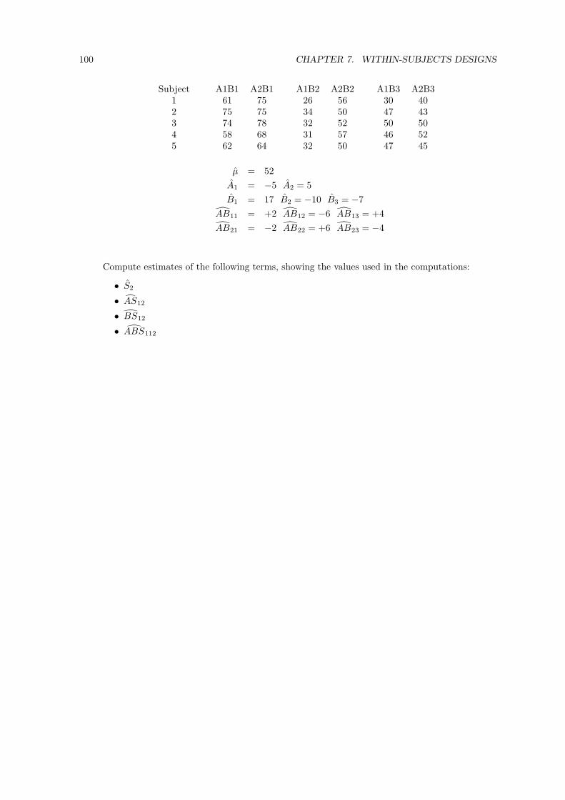
100 CHAPTER 7. WITHIN-SUBJECTS DESIGNS
Subject A1B1 A2B1 A1B2 A2B2 A1B3 A2B31 61 75 26 56 30 402 75 75 34 50 47 433 74 78 32 52 50 504 58 68 31 57 46 525 62 64 32 50 47 45
µ = 52
A1 = −5 A2 = 5
B1 = 17 B2 = −10 B3 = −7
AB11 = +2 AB12 = −6 AB13 = +4
AB21 = −2 AB22 = +6 AB23 = −4
Compute estimates of the following terms, showing the values used in the computations:
• S2
• AS12
• BS12
• ABS112

7.9. ANSWERS TO EXERCISES 101
7.9 Answers to Exercises
1.
Source: Error Termµ SA ASB BS
AB ABSC CS
AC ACSBC BCS
ABC ABCSS
ASBS
ABSCS
ACSBCS
ABCS
2.
(a) The three factors are Gravity Condition, Time Since Sleep, and Astronaut, and all arefixed-effects factors. In particular, Astronaut cannot be a random-effects factor, becausethe levels (i.e., astronauts) were not sampled randomly, nor is there any intent to generalizethe results to a larger population of astronauts.
(b) The extent to which overall performance is different in the three gravity conditions.
(c) The extent to which overall performance is different for the six different astronauts.
(d) The extent to which the effect of gravity condition on performance is different dependingon the time since sleep (or vice versa).
(e) The extent to which the effect of gravity condition on performance is different for thedifferent astronauts.
(f) The extent to which the interaction of gravity condition and time since sleep is differentfor the different astronauts.
(g) The True/False questions are all false.
3.
• S2 = 2
• AS12 = 3
• BS12 = 4
• ABS112 = 0

102 CHAPTER 7. WITHIN-SUBJECTS DESIGNS

Chapter 8
Mixed Designs—The General Case
Now that you know how to analyze designs with between-subjects factors and designs with within-subjects factors, it is time to consider designs with both types of factors in the same experiment.Such designs are the topic of this section. Mixed designs are very common, because most dependentvariables depend both on factors that vary between subjects and on factors that vary within subjectsacross time. The simplest mixed design has two factors—one within and one between. For example, aresearcher might compare GPAs for males vs. females in math vs. language courses. Gender would bea between-subjects factor, of course. If both math and language GPAs were obtained for each subject,the Course factor would be within-subjects. Obviously, a more complicated mixed design could bedeveloped from this example by adding factors. A second between-subjects factor might be Class level(freshman, sophomore, junior, senior), and a third might be university (Harvard, Berkeley, SlipperyRock). An additional within-subjects factor could be Time of Day (assuming that each student hadat least one course of each type in the morning and another in the afternoon). And so on.
The same steps are needed to analyze mixed designs as to analyze between- and within-subjectsdesigns:
• Write down the model.
• Write down the estimation equations.
• Obtain SS′s, either by estimating individual values and forming the decomposition matrix orby using the shortcut method.
• Determine the values of degrees of freedom.
• Select the appropriate error term(s) and compute Fobserved’s.
Thus, in this chapter we will see how to merge the methods of the previous analyses for designswith all factors between- or within-subjects. In fact, the rules to be developed in this chapter aregeneralizations of both sets of rules developed previously. This means that you can use the rulesstated here to analyze between-subjects designs or within-subjects designs, in addition to the mixeddesigns.
To illustrate the rules we develop, we will discuss two examples throughout the chapter. In boththese examples, a physician is interested in the dependent variable of heart rate. The simpler examplehas only two factors: Age (between-subjects) and presence vs. absence of a new drug being tested(within-subjects). The data for this example are shown in Table 8.1. The more complex exampleaugments this design with the between-subjects factor of Gender and the within-subjects factor ofStress Level (i.e., sleeping vs. walking on a treadmill). The data for this example appear in Table 8.2,and the corresponding cell and marginal means are shown in Table 8.3.
8.1 Linear Model
Table 8.4 shows the general rules for constructing a linear model. These rules are general enoughto apply to the mixed designs considered in this chapter; they also work for entirely between- orwithin-subjects designs considered in earlier chapters.
Following the rules in this table, the model for the Age x Drug design is:
Yijk = µ + Ai + Bj + ABij + S(A)ik + BS(A)ijk
103

104 CHAPTER 8. MIXED DESIGNS—THE GENERAL CASE
Old Subjects Young SubjectsSubject No Drug Drug Subject No Drug Drug
1 73 59 1 61 632 81 67 2 60 503 86 60 3 59 61
Cell Means:Age: No Drug DrugOld 80 62Young 60 58
Table 8.1: Example Data Illustrating Dependence of Heart Rate on Age (Factor A, between-Ss) andDrug (Factor B, within-Ss)
Old MalesNo Drug Drug
Subject Treadmill Sleep Treadmill Sleep1 131 73 41 472 121 83 47 41
Average 126 78 44 44Old Females
No Drug DrugSubject Treadmill Sleep Treadmill Sleep
1 101 71 45 592 75 65 23 49
Average 88 68 34 54Young Males
No Drug DrugSubject Treadmill Sleep Treadmill Sleep
1 100 64 52 482 112 84 36 56
Average 106 74 44 52Young Females
No Drug DrugSubject Treadmill Sleep Treadmill Sleep
1 71 61 31 412 89 59 45 59
Average 80 60 38 50
Table 8.2: Example Data Illustrating Dependence of Heart Rate on Age (Factor A, between-Ss), Drug(Factor B, within-Ss), Gender (Factor C, between-Ss), and Stress (Factor D, within-Ss)
and the model for the Age x Drug x Gender x Stress design is:
Yijklm = µ + Ai + Bj + ABij + Ck + ACik + BCjk + ABCijk
+Dl + ADil + BDjl + ABDijl + CDkl + ACDikl + BCDjkl + ABCDijkl
+S(AC)ikm + BS(AC)ijkm + DS(AC)iklm + BDS(AC)ijklm
These models deserve a little discussion. There is nothing surprising in the presence of µ orthe main effects and interactions involving the regular experimental factors (i.e., A, B, C, and D).Such terms are at least somewhat familiar because they had the same form in both between- andwithin-subjects designs, and they retain the same meaning in mixed designs.
The novel feature of these models is the pattern of subjects terms. In between-subjects designsthere was a single subjects term, with all the factors listed after it in parentheses. In within-subjectsdesigns there was an S term with no parentheses, and there were also interactions of S with all of theother factors. Here we follow both rules at once: The between-subjects factors are listed in parenthesesafter S, and the S term appears in interactions with all of the within-subjects factors.
There is nothing mysterious about these rules involving the subject term—on the contrary, theirconceptual basis is quite straightforward. In all cases, the terms in the model simply reflect the typesof information that are available from the experimental design.

8.1. LINEAR MODEL 105
No Drug DrugTread Sleep Tread Sleep
Old 107 73 39 49Young 93 67 41 51Average 100 70 40 50
Male FemaleTread Sleep Tread Sleep
No Drug 116 76 84 64Drug 44 48 36 52Average 80 62 60 58
Old YoungMale Female Male Female
Tread 85 61 75 59Sleep 61 61 63 55Average 73 61 69 57
Old YoungNo Drug Drug Mo Drug Drug
Male 102 44 90 48Female 78 44 70 44Average 90 44 80 46
Old Young AverageTread 73 67 70Sleep 61 59 60Average 67 63 65
Male Female AverageNo Drug 96 74 85Drug 46 44 45Average 71 59 65
Table 8.3: Means and Marginal Means for Data of Table 8.2.
• Y has one subscript for each experimental factor, between or within, and one for subjects.
• There is a µ term.
• There is a main effect term A, B, C, . . . for each experimental factor, between or within.
• There are all possible two-way, three-way, four-way, . . . interaction terms that can be constructedfrom subsets of the experimental factors.
• There is a subjects term, S, which is written with a list of the between-subjects factors insideparentheses.
• There are terms for the interactions of subjects with every within-subjects factor and everyinteraction involving only within-subjects factors.
Table 8.4: General Rules for Constructing ANOVA Models
Consider the simpler design first.
• There is a S(A)ik term, because the design allows us to estimate the specific effect on each scoredue to the particular randomly sampled subject from whom that score was obtained. We denotethis effect by S(A)ik so that the notation will reflect the fact that Young Subject 1 is a differentindividual than Old Subject 1 (and may therefore have a different effect).
• There is a BS(A)ijk term, because the design allows us to estimate the relative responsivenessof each individual to the two drug conditions. The design allows this because each subject istested both with and without the drug. If Joe shows little effect of the drug whereas Sam showsa big effect, for example, then the values of BS(A)ijk will be near-zero for Joe and far-from-zerofor Sam. In short, this is the model term that shows us how much the drug effect varies fromperson to person—a type of information that is always present for any within-subjects factor.
• The model does not contain an AS(A) term, which could potentially measure the responsivenessof each individual subject to the Age factor (i.e., the interaction of Age and Subject). The reasonis quite clear: Since each subject was only measured in one age group, it is impossible to comparethe responses of different subjects to the change in age.
In a nutshell: Models for mixed designs include terms for the interaction of subjects with within-subjects factors, because it is possible to see how within-subjects effects differ from subject to subject.Models for mixed designs do not include terms for the interaction of subjects with between-subjects

106 CHAPTER 8. MIXED DESIGNS—THE GENERAL CASE
factors, because it is impossible to see between-subjects effects on an individual subject (and thereforeit is impossible to see how they differ from subject to subject).
The same principles apply to the more complex design. All of the standard experimental factors(A, B, C, and D) and their interactions are included in the model, because we can estimate the effectsof these factors, as in any factorial experiment. Likewise, there is a term to indicate the effect ofthe particular subject in each group; this time, the four groups of subjects are differentiated by twobetween-subjects factors. In addition, there are two two-way interaction terms involving subjects:BS(AC)ijkm and DS(AC)iklm . The first indicates any special effect of Drug on a subject, and it isincluded because having Drug as a within-subjects factor enables us to measure the effect of Drugseparately for each subject. The second indicates any special effect of Stress on a subject, and it isincluded because having Stress as a within-subjects factor enables us to measure the effect of Stressseparately for each subject.
Finally, there is a three-way interaction term involving the two within-subjects factors, togetherwith subjects: BDS(AC)ijklm . The justification for this term was already given in the chapter onwithin-subjects designs: The design allows us to estimate the BD interaction separately for eachsubject, so the term will indicate the size of the BD interaction for each subject. As before, we canuse this term to see how the BD interaction varies from subject to subject.
It is also worth discussing the terms that are missing from the model for the complex example.For example, the Age by subjects interaction term is missing, for the same reason as in the simplerexample: we cannot estimate the effect of age on an individual subject in this design (to do so wouldrequire testing the same subject in both age groups). The same comment applies to the Gender bysubjects interaction and the Age by Gender interaction.
More interesting is the absence of the Age by Drug by subjects interaction. Age is between-subjects, but Drug is within—so why is the three-way interaction missing? As always, the rule isthat the interaction is missing because the design does not allow us to estimate it. In this case, tomeasure the Age by Drug by Subjects interaction we would have to be able to measure the Age byDrug interaction separately for each subject. We can so measure the Drug effect—Drug being a withinfactor—but not the change in Drug effect with age (i.e., the Drug x Age interaction). Because eachsubject is observed in only one age group, it is impossible to see how the effect of drug changes withage for that subject. Thus, the design does not allow measurement of the Drug x Age x Subjectsinteraction, and the term is not included in the model.
A little reflection shows that the points made about the factors of these examples apply in generalto all within- and between-subject factors. Thus, these ideas really justify the general rules for thelinear model given in Table 8.4.
8.2 Estimation Equations and SS’s
For mixed designs, estimation proceeds just as it did for between- and within-subject designs.
• For any term, the estimation equation has the form:
Estimate of Term = Data Average - Estimates of Subterms
• The data average has the same subscripts as those on the term to be estimated, and it is averagedover all the subscripts absent from that term.
• The subterms of a term are those simpler terms that are logically contained within the term.More formally, term “Sub” is a subterm of term “Super” if every subscript on term “Sub” isalso a subscript on term “Super.” µ is a subterm of every other term.
Tables 8.5 and 8.6 show the estimation equations for the simple and complex examples involvingthe dependent variable of heart rate. It is easy to see that there are no new principles at workhere, although the complicated nature of the model terms may at first cause confusion. It is alwayspossible to get the right answer, though, by working from left to right through the model and checkingsubscripts carefully.
Once the estimation equations have been written down, it is a simple though often very tediousmatter to compute the SS for each term in the model. This can be done either by estimating eachindividual term and writing down the decomposition matrix (see examples in Tables 8.7, 8.8, and 8.9),or by using the shortcut method.

8.3. DEGREES OF FREEDOM 107
µ = Y...
Ai = Yi.. − µ
Bj = Y.j. − µ
ABij = Yij. − µ − Ai − Bj
S(A)ik = Yi.k − µ − Ai
BS(A)ijk = Yijk − µ − Ai − Bj − ABij − S(A)ik
Table 8.5: Estimation Equations for the Simple Design of Table 8.1
8.3 Degrees of Freedom
The rules for computing degrees of freedom are also quite familiar.
• dfµ = 1.
• The main effect of a factor with K levels has K − 1 df.
• The number of df’s for the main effect of subjects is again the number of subjects minus thenumber of groups. The number of groups is the product of the numbers of levels of all thebetween-Ss factors.
• Interaction df’s are found by multiplying together the df’s of the associated main effects.
• dftotal = the number of data values.
Note that these rules also give the correct df values for between- and within-subject designs.
8.4 Error Terms
A surprisingly simple rule describes the proper selection of error terms for computing Fobserved’s inmixed designs as well as between- and within-subjects designs:
To compute the Fobserved with any given source in the numerator, use in the denominatorthe source which is the interaction of subjects by all of the within-subjects factors containedin the source in the numerator.
Before discussing mixed designs, we hasten to point out that this rule also applies to between-and within-subjects designs; that is, it gives the same error terms for these designs as we describedin previous chapters. In between-subjects designs, for example, “the interaction of subjects by all ofthe within-subjects factors . . . ” is simply the subjects term used to compute all Fobserved’s. Thisis because there are no within-subjects factors in any source, and the interaction of “subjects bynothing” is just “subjects.” Conversely, in within-subjects designs, “the interaction of subjects by allof the within-subjects factors . . . ” is simply the numerator by subjects interaction term, because allof the factors in the numerator are necessarily within-subjects. As we have already seen in Chapter 7,this is the appropriate error term.
Now to mixed designs. Tables 8.10 and 8.11 show the ANOVA tables for the two examples beingdiscussed in this chapter, and it worth examining the pattern of the error terms to see how they aregenerated by the rule. You can see that, for any given source, the error term is simply the interactionof subjects with the within-subjects factors contained in the source.
Of course we must also discuss the rationales behind the error terms, in order to justify the rule.For main effects, the rationales are pretty familiar. According to the rule, we use subjects (i.e., thesubjects by nothing interaction) as the error term for a between-subjects main effect. As noted inthe chapters on between-subjects designs, this is because the subjects term is a measure of how muchdifference we can expect between subjects in the same condition(s), and this difference tells us howlarge the between-group differences might be due to chance. Conversely, we use the subject by factorinteraction as the error term for a within-subjects main effect. As noted in the chapter on within-subjects designs, this is because the subject by factor interaction is a measure of how inconsistent the

108 CHAPTER 8. MIXED DESIGNS—THE GENERAL CASE
µ = Y.....
Ai = Yi.... − µ
Bj = Y.j... − µ
ABij = Yij... − µ − Ai − Bj
Ck = Y..k.. − µ
ACik = Yi.k.. − µ − Ai − Ck
BCjk = Y.jk.. − µ − Bj − Ck
ABCijk = Yijk.. − µ − Ai − Bj − ABij − Ck − ACik − BCjk
Dl = Y...l. − µ
ADil = Yi..l. − µ − Ai − Dl
BDjl = Y.j.l. − µ − Bj − Dl
ABDijl = Yij.l. − µ − Ai − Bj − ABij − Dl − ADil − BDjl
CDkl = Y..kl. − µ − Ck − Dl
ACDikl = Yi.kl. − µ − Ai − Ck − ACik − Dl − ADil − CDkl
BCDjkl = Y.jkl. − µ − Bj − Ck − BCjk − Dl − BDjl − CDkl
ABCDijkl = Yijkl. − µ − Ai − Bj − ABij − Ck − ACik − BCjk
−Dl − ADil − BDjl − ABDijl − CDkl − ACDikl − BCDjkl
S(AC)ikm
= Yi.k.m − µ − Ai − Ck − ACik
BS(AC)ijkm
= Yijk.m − µ − Ai − Bj − ABij − Ck − ACik − BCjk − ABCijk −S(AC)
ikm
DS(AC)iklm
= Yi.klm − µ − Ai − Ck − ACik − Dl − ADil − CDkl − ACDikl −S(AC)
ikm
BDS(AC)ijklm
= Yijklm − µ − Ai − Bj − ABij − Ck − ACik − BCjk − ABCijk − Dl
−ADil − BDjl − ABDijl − CDkl − ACDikl − BCDjkl −ABCDijkl
−S(AC)ikm −
BS(AC)ijkm −DS(AC)iklm
Table 8.6: Estimation Equations for the Complex Design of Table 8.2
effect is across subjects, and because our confidence in the reality of an effect is inversely related to itsinconsistency across subjects (i.e., the more consistent it is across subjects, the more confident we arethat it’s real). The rationales are also familiar for interactions that are entirely between-subjects (i.e.,involve only between-subjects factors) or entirely within-subjects (i.e., involve only within-subjectsfactors). In the former case we are interested in the size of between-group differences that might ariseby chance, and “subjects” is the relevant error term because it measures the inconsistency betweensubjects within a given condition. In the latter case we are interested in the (in)consistency of theinteraction in question across subjects, and the “subjects by interaction” error term measures this forus.
To summarize: For entirely between main effects or interactions, we use the same error term thatwe would use if none of the within-subjects factors had been included in the design. For entirelywithin main effects or interactions, we use the same error term that we would use if none of thebetween-subjects factors had been included in the design. This makes some intuitive sense, sinceincluding extra factors in the design and analysis doesn’t really change the nature of the informationwe have about any given factor.
The new and somewhat tricky case involves interactions including both between- and within-subjects factors. In the simple example, for instance, we need an error term for the Age (between) byDrug (within) interaction. In the complex example, we need error terms for this same interaction plusa variety of other “mixed” ones (e.g., Age x Drug x Gender, Age x Drug x Gender x Stress). The rulefor these cases is quite clear of course—use the “subjects by within” interactions for the error terms.But what is the rationale?
The rationale is subtle: The design allows us to measure how much the within-subjects effect variesrandomly from person to person. Therefore, in order to see whether the within-subjects effect really

8.5. ORDER EFFECTS 109
Yijk = µ + Ai + Bj + ABij + S(A)ik + BS(A)ijk
73 = 65 + 5 + 6 + 4 - 5 - 259 = 65 - 5 + 6 - 4 - 5 + 281 = 65 + 5 + 6 + 4 + 3 - 267 = 65 - 5 + 6 - 4 + 3 + 286 = 65 + 5 + 6 + 4 + 2 + 460 = 65 - 5 + 6 - 4 + 2 - 461 = 65 + 5 - 6 - 4 + 3 - 263 = 65 - 5 - 6 + 4 + 3 + 260 = 65 + 5 - 6 - 4 - 4 + 450 = 65 - 5 - 6 + 4 - 4 - 459 = 65 + 5 - 6 - 4 + 1 - 261 = 65 - 5 - 6 + 4 + 1 + 2
Table 8.7: Decomposition Matrix for the Data of Table 8.1
varies between groups, we need to see whether the group-to-group variation in the effect is larger thanwe can explain in terms of random person-to-person variation in the effect.
In the simple design, for example, we note that the drug effect is somewhat different for the Oldpeople (18 beats per minute) than for the Young people (2 beats per minute). This seems like alarge effect, but to be sure we must compare it to the person-to-person random variation in the Drugeffect—that is, to the Drug by Subjects(Age) interaction term. If there were enough random variationin the size of the drug effect among both the young and the old subjects, perhaps we would decidethat the difference between 18 and 2 could just be random error.
A more elaborate version of the same basic rationale explains the selection of error terms in thecomplex data set as well. Consider the most difficult examples: the three and four way interactionsincluding Drug by Stress. Now the Drug by Stress interaction is measured within-subjects, so themodel allows us to estimate the extent to which this interaction varies from subject to subject.Furthermore, this estimate provides an index of the amount of random variation in the Drug byStress interaction. Naturally, then, when we want to see whether the Drug by Stress interaction isdifferent for Males vs. Females (i.e., test Gender x Drug x Stress), we compare the size of the three-wayinteraction against this index of random variation in the Drug x Stress interaction. The same ideajustifies testing both Age x Drug x Stress and Age x Gender x Drug x against the Drug x Stress xSubjects interaction.1
8.5 Order Effects
We close this chapter with a discussion of an example involving the use of a mixed design to allowfor order effects on a within-subjects factor.2 As noted in Section 7.1, an apparent disadvantage ofwithin-subjects testing is that the process of testing a subject in one condition may produce seriouschanges that affect the results in conditions tested later. Consider, for example, an experiment inwhich we seek to determine the effect of alcohol on motor coordination. A test of motor coordinationis given to each subject twice—once under the influence of alcohol and once not under the influence.Clearly, we would have to worry about the possibility of order effects, because subjects might show ageneral improvement at the second test of coordination, just due to learning.
One obvious experimental precaution would be to test different groups of subjects in differentorders. We would want to test half of the subjects first in the No-Alcohol condition and then in theAlcohol condition, with the other half of the subjects tested in the reverse order. This experimentalprecaution is known as counterbalancing order, and it is needed to prevent confounding order withAlcohol vs. No-Alcohol, as would happen if all subjects were tested in the same order.
1Our discussion here focuses on the Drug x Stress interaction and how it changes across levels of other factors (e.g.,Gender). Some readers, remembering the symmetric nature of interactions, may wonder whether the discussion couldjust as well have focused on (say) the Gender by Drug interaction and how it changed across levels of Stress. The answeris “no”, and this is one sense in which interactions fail to be completely symmetric. Whereas interactions are completelysymmetric with respect to their interpretations, they are asymmetric with respect to their error terms, because the errorterm always involves the random variability in the within-subjects component.
2Such effects are sometimes called carry-over effects.

110 CHAPTER 8. MIXED DESIGNS—THE GENERAL CASE
Yijklm = µ +Ai +Bj +ABij +Ck +ACik +BCjk +ABCijk +Dl +ADil +BDjl +ABDijl + . . .131 =65+ 5 + 20 + 10 + 6 + 4 + 5 + 1 + 2 + 1 + 3 + 1 + . . .73 =65 - 5 + 20 - 10 + 6 - 4 + 5 - 1 + 2 - 1 + 3 - 1 + . . .41 =65+ 5 - 20 - 10 + 6 + 4 - 5 - 1 + 2 + 1 - 3 - 1 + . . .47 =65 - 5 - 20 + 10 + 6 - 4 - 5 + 1 + 2 - 1 - 3 + 1 + . . .121 =65+ 5 + 20 + 10 + 6 + 4 + 5 + 1 + 2 + 1 + 3 + 1 + . . .83 =65 - 5 + 20 - 10 + 6 - 4 + 5 - 1 + 2 - 1 + 3 - 1 + . . .47 =65+ 5 - 20 - 10 + 6 + 4 - 5 - 1 + 2 + 1 - 3 - 1 + . . .41 =65 - 5 - 20 + 10 + 6 - 4 - 5 + 1 + 2 - 1 - 3 + 1 + . . .101 =65+ 5 + 20 + 10 - 6 - 4 - 5 - 1 + 2 + 1 + 3 + 1 + . . .71 =65 - 5 + 20 - 10 - 6 + 4 - 5 + 1 + 2 - 1 + 3 - 1 + . . .45 =65+ 5 - 20 - 10 - 6 - 4 + 5 + 1 + 2 + 1 - 3 - 1 + . . .59 =65 - 5 - 20 + 10 - 6 + 4 + 5 - 1 + 2 - 1 - 3 + 1 + . . .75 =65+ 5 + 20 + 10 - 6 - 4 - 5 - 1 + 2 + 1 + 3 + 1 + . . .65 =65 - 5 + 20 - 10 - 6 + 4 - 5 + 1 + 2 - 1 + 3 - 1 + . . .23 =65+ 5 - 20 - 10 - 6 - 4 + 5 + 1 + 2 + 1 - 3 - 1 + . . .49 =65 - 5 - 20 + 10 - 6 + 4 + 5 - 1 + 2 - 1 - 3 + 1 + . . .100 =65+ 5 + 20 + 10 + 6 + 4 + 5 + 1 - 2 - 1 - 3 - 1 + . . .64 =65 - 5 + 20 - 10 + 6 - 4 + 5 - 1 - 2 + 1 - 3 + 1 + . . .52 =65+ 5 - 20 - 10 + 6 + 4 - 5 - 1 - 2 - 1 + 3 + 1 + . . .48 =65 - 5 - 20 + 10 + 6 - 4 - 5 + 1 - 2 + 1 + 3 - 1 + . . .112 =65+ 5 + 20 + 10 + 6 + 4 + 5 + 1 - 2 - 1 - 3 - 1 + . . .84 =65 - 5 + 20 - 10 + 6 - 4 + 5 - 1 - 2 + 1 - 3 + 1 + . . .36 =65+ 5 - 20 - 10 + 6 + 4 - 5 - 1 - 2 - 1 + 3 + 1 + . . .56 =65 - 5 - 20 + 10 + 6 - 4 - 5 + 1 - 2 + 1 + 3 - 1 + . . .71 =65+ 5 + 20 + 10 - 6 - 4 - 5 - 1 - 2 - 1 - 3 - 1 + . . .61 =65 - 5 + 20 - 10 - 6 + 4 - 5 + 1 - 2 + 1 - 3 + 1 + . . .31 =65+ 5 - 20 - 10 - 6 - 4 + 5 + 1 - 2 - 1 + 3 + 1 + . . .41 =65 - 5 - 20 + 10 - 6 + 4 + 5 - 1 - 2 + 1 + 3 - 1 + . . .89 =65+ 5 + 20 + 10 - 6 - 4 - 5 - 1 - 2 - 1 - 3 - 1 + . . .59 =65 - 5 + 20 - 10 - 6 + 4 - 5 + 1 - 2 + 1 - 3 + 1 + . . .45 =65+ 5 - 20 - 10 - 6 - 4 + 5 + 1 - 2 - 1 + 3 + 1 + . . .59 =65 - 5 - 20 + 10 - 6 + 4 + 5 - 1 - 2 + 1 + 3 - 1 + . . .
Table 8.8: Part 1 of Decomposition Matrix for the Data of Table 8.2
It is not enough just to counterbalance order in the experimental design—we must also take orderinto account in the statistical analysis. Mixed designs are very useful in examining order effects.Include in the design a between-subjects factor defined by the different orders in which the differentgroups of subjects are tested across the levels of the within-subjects factor(s). The model terms forthis factor will allow for an effect of order on overall performance level and an effect of order on thesize of the experimental effects (e.g., Alcohol). In most cases, these terms will help to reduce the errorterms, because any large effects of or interactions with Order will go into these error terms if Orderis not included as a factor in the design.
It may at first seem undesirable to include Order in the analysis, because in most cases order isprobably not a factor that we as experimenters would have any interest in. Nonetheless, it would be amistake to omit Order from the analysis, because doing so could well inflate the error term(s) for theeffects we were interested in. Besides, order effects and their interactions might turn out to be moreinteresting than we realized ahead of time. If the experiment provides information on order effects,why not look to see what the results are?
Data for this example are presented in Table 8.12, with 2 groups containing 4 subjects per group.The model is a the standard model for a mixed design with one between- and one within-subjectsfactor:
Yijk = µ + Ai + Bj + ABij + S(B)jk + AS(B)ijk
where A is the term for the Alcohol factor and B is the term for the Order factor.The ANOVA table for this example is shown in Table 8.13. The effect of Alcohol is clearly
significant, indicating that there is an effect of alcohol on motor coordination. Interestingly, there isalso a big interaction of Alcohol and Order. Looking at the means, we see that the Alcohol effect ismuch larger for those tested with Alcohol first and No-Alcohol second than for those tested in thereverse order. This probably just means that there is a substantial practice effect, upon which the

8.5. ORDER EFFECTS 111
. . . +CDkl +ACDikl +BCDjkl +ABCDijkl +S(AC)ikm +BS(AC)ijkm +DS(AC)iklm +BDS(AC)ijklm
. . . + 0 + 2 + 1 + 0 + 0 + 1 + 0 + 4
. . . + 0 - 2 + 1 + 0 + 0 - 1 + 0 - 4
. . . + 0 + 2 - 1 + 0 + 0 + 1 + 0 - 4
. . . + 0 - 2 - 1 + 0 + 0 - 1 + 0 + 4
. . . + 0 + 2 + 1 + 0 + 0 - 1 + 0 - 4
. . . + 0 - 2 + 1 + 0 + 0 + 1 + 0 + 4
. . . + 0 + 2 - 1 + 0 + 0 - 1 + 0 + 4
. . . + 0 - 2 - 1 + 0 + 0 + 1 + 0 - 4
. . . + 0 - 2 - 1 + 0 + 8 + 4 + 0 + 1
. . . + 0 + 2 - 1 + 0 + 8 - 4 + 0 - 1
. . . + 0 - 2 + 1 + 0 + 8 + 4 + 0 - 1
. . . + 0 + 2 + 1 + 0 + 8 - 4 + 0 + 1
. . . + 0 - 2 - 1 + 0 - 8 - 4 + 0 - 1
. . . + 0 + 2 - 1 + 0 - 8 + 4 + 0 + 1
. . . + 0 - 2 + 1 + 0 - 8 - 4 + 0 + 1
. . . + 0 + 2 + 1 + 0 - 8 + 4 + 0 - 1
. . . + 0 - 2 - 1 + 0 - 3 + 4 - 5 - 2
. . . + 0 + 2 - 1 + 0 - 3 - 4 - 5 + 2
. . . + 0 - 2 + 1 + 0 - 3 + 4 + 5 + 2
. . . + 0 + 2 + 1 + 0 - 3 - 4 + 5 - 2
. . . + 0 - 2 - 1 + 0 + 3 - 4 + 5 + 2
. . . + 0 + 2 - 1 + 0 + 3 + 4 + 5 - 2
. . . + 0 - 2 + 1 + 0 + 3 - 4 - 5 - 2
. . . + 0 + 2 + 1 + 0 + 3 + 4 - 5 + 2
. . . + 0 + 2 + 1 + 0 - 6 - 2 + 2 - 3
. . . + 0 - 2 + 1 + 0 - 6 + 2 + 2 + 3
. . . + 0 + 2 - 1 + 0 - 6 - 2 - 2 + 3
. . . + 0 - 2 - 1 + 0 - 6 + 2 - 2 - 3
. . . + 0 + 2 + 1 + 0 + 6 + 2 - 2 + 3
. . . + 0 - 2 + 1 + 0 + 6 - 2 - 2 - 3
. . . + 0 + 2 - 1 + 0 + 6 + 2 + 2 - 3
. . . + 0 - 2 - 1 + 0 + 6 - 2 + 2 + 3
Table 8.9: Part 2 of Decomposition Matrix for the Data of Table 8.2
alcohol effect is superimposed. Alternatively, it may mean that the effect of alcohol truly does dependon previous experience with the task. These data do not decide that question. But they do show thatAlcohol has at least some effect, and they demonstrate this with order taken into account.
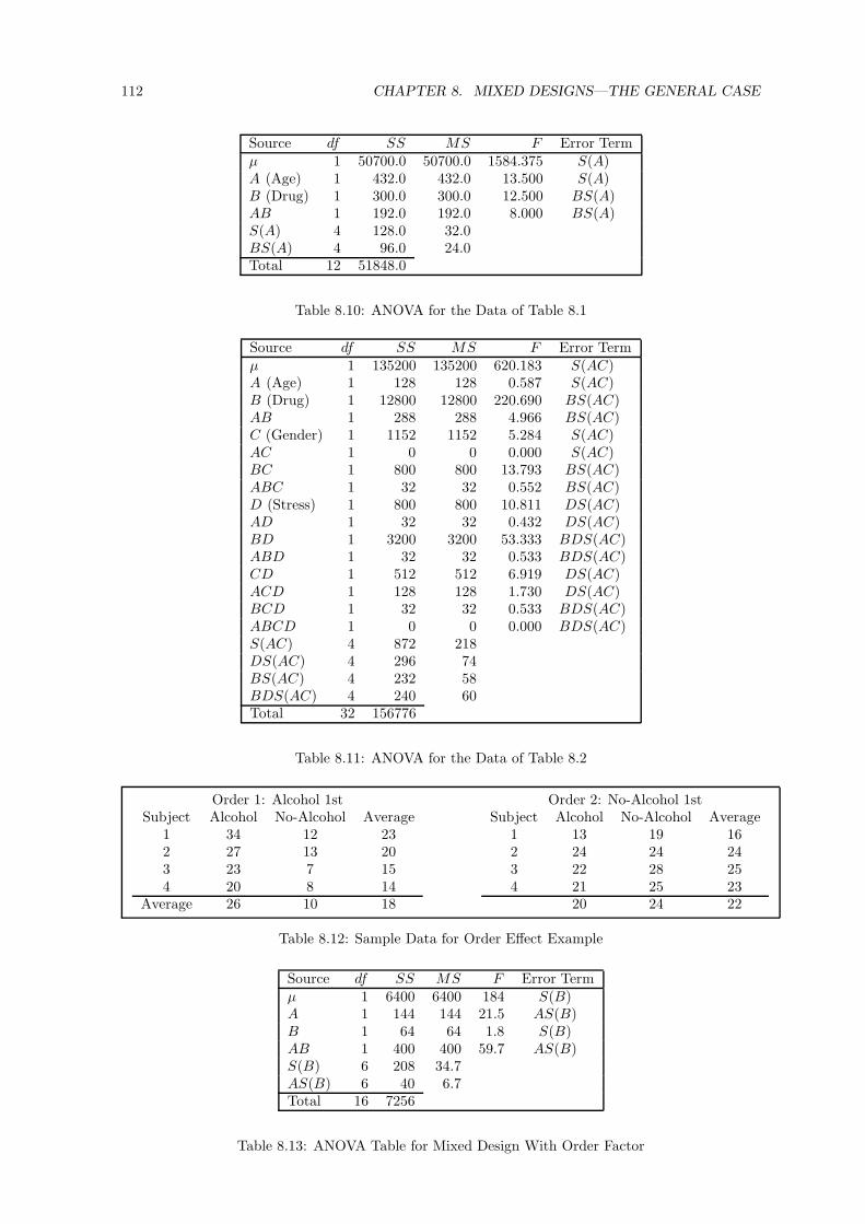
112 CHAPTER 8. MIXED DESIGNS—THE GENERAL CASE
Source df SS MS F Error Termµ 1 50700.0 50700.0 1584.375 S(A)A (Age) 1 432.0 432.0 13.500 S(A)B (Drug) 1 300.0 300.0 12.500 BS(A)AB 1 192.0 192.0 8.000 BS(A)S(A) 4 128.0 32.0BS(A) 4 96.0 24.0Total 12 51848.0
Table 8.10: ANOVA for the Data of Table 8.1
Source df SS MS F Error Termµ 1 135200 135200 620.183 S(AC)A (Age) 1 128 128 0.587 S(AC)B (Drug) 1 12800 12800 220.690 BS(AC)AB 1 288 288 4.966 BS(AC)C (Gender) 1 1152 1152 5.284 S(AC)AC 1 0 0 0.000 S(AC)BC 1 800 800 13.793 BS(AC)ABC 1 32 32 0.552 BS(AC)D (Stress) 1 800 800 10.811 DS(AC)AD 1 32 32 0.432 DS(AC)BD 1 3200 3200 53.333 BDS(AC)ABD 1 32 32 0.533 BDS(AC)CD 1 512 512 6.919 DS(AC)ACD 1 128 128 1.730 DS(AC)BCD 1 32 32 0.533 BDS(AC)ABCD 1 0 0 0.000 BDS(AC)S(AC) 4 872 218DS(AC) 4 296 74BS(AC) 4 232 58BDS(AC) 4 240 60Total 32 156776
Table 8.11: ANOVA for the Data of Table 8.2
Order 1: Alcohol 1st Order 2: No-Alcohol 1stSubject Alcohol No-Alcohol Average Subject Alcohol No-Alcohol Average
1 34 12 23 1 13 19 162 27 13 20 2 24 24 243 23 7 15 3 22 28 254 20 8 14 4 21 25 23
Average 26 10 18 20 24 22
Table 8.12: Sample Data for Order Effect Example
Source df SS MS F Error Termµ 1 6400 6400 184 S(B)A 1 144 144 21.5 AS(B)B 1 64 64 1.8 S(B)AB 1 400 400 59.7 AS(B)S(B) 6 208 34.7AS(B) 6 40 6.7Total 16 7256
Table 8.13: ANOVA Table for Mixed Design With Order Factor

Chapter 9
Shortcut for Computing Sums ofSquares
This chapter explains how to use a computational shortcut for getting sums of squares. Basically, itis possible to get the sums of squares without obtaining the numerical estimates for all of the termsin the model, as is required to obtain SS’s from the decomposition matrix. Since you don’t actuallyhave to estimate each term in the model, you save a lot of subtractions.
This computational shortcut is not given in the earlier chapters because it does not promoteintuitive understanding. We present it here in spite of this major defect, just in case you are evercaught away from a computer and want to do a sizeable ANOVA by hand.
The computational shortcut works for all equal cell size designs: between-subjects, within-subjects,and mixed. Before you can use it, though, you must first be able to write out the model. Then, tocompute the SS for any term in the model:
1. Write out its estimation equation, which has the form:
Term = Data average - estimates of other model terms
2. Write out the corresponding shortcut equation, which has the form:
SSTerm = n ×∑
(Data average2) − SS′s for other model terms
To construct and use this equation you need to know two things:
• n is the number of scores that are averaged together to compute each of the data averagesto which the equation refers.
• The “other model terms” for which you subtract off the SS’s are the very same terms forwhich you subtract off estimates in the corresponding estimation equation.
That is all there is to it.
9.1 One-Factor Between-Ss Example
To illustrate the shortcut in the simplest case, we will use it to get SS’s for the data of Section 3.10.The model is:
Yij = µ + Ai + S(A)ij
and so we only need to compute SSµ, SSA, and SSS(A).
µ: The estimation equation isµ = Y..
Thus, the corresponding shortcut SS equation is
SSµ = n × Y..2
• n is 12, because Y.. is an average over 12 data values.
113

114 CHAPTER 9. SHORTCUT FOR COMPUTING SUMS OF SQUARES
• No “other model terms” are subtracted from the data value in the estimation equation, so noSS’s are subtracted in the shortcut equation.
Substituting in the numbers gives
SSµ = 12 × 302 = 10, 800
A: The estimation equation isAi = Yi. − µ
Thus, the corresponding shortcut SS equation is
SSA = n ×∑
(Yi.2) − SSµ
• n is 3, because each Yi. is an average over 3 data values.
• µ is subtracted from the data value in the estimation equation, so SSµ is subtracted in theshortcut equation.
Thus,SSA = 3 × (402 + 342 + 242 + 222) − 10, 800 = 648
S(A): The estimation equation is
S(A)i = Yij − µ − Ai
Thus, the corresponding shortcut SS equation is
SSS(A) = n ×∑
(Yij2) − SSµ − SSA
• n is 1, because each Yij is an average over 1 data value (i.e., it is just a data value).
• µ and Ai are subtracted from the data value in the estimation equation, so SSµ and SSA aresubtracted in the shortcut equation.
Thus,
SSS(A) = (392 + 412 + 402 + 352 + 352 + 322 + 242 + 252 + 232 + 222 + 232 + 212)
−10, 800− 648
= 12
9.2 Three-Factor Between-Ss Example
Table 9.1 shows sample data from an experiment examining the amount learned by students as afunction of their own gender, the gender of their teachers, and the type of courses being taken (sciencevs. language). The cell and marginal means are also shown.
To compute the SS’s with the shortcut method, proceed as follows:
µ: The estimation equation is:µ = Y....
The corresponding shortcut equation is therefore:
SSµ = n × Y....2
with n = 24, because 24 data values were averaged together to get Y..... Thus,
SSµ = 24 × 1002 = 240, 000

9.2. THREE-FACTOR BETWEEN-SS EXAMPLE 115
Data:Science Courses
Students Male Teachers Female TeachersMale 101 99 103 101 105 97Female 90 92 97 91 96 92
Language CoursesStudents Male Teachers Female TeachersMale 109 107 105 97 99 101Female 99 94 92 114 114 105
Cell Means:Science Courses
Students: Male Teachers Female TeachersMale 101 101Female 93 93
Language CoursesStudents: Male Teachers Female TeachersMale 107 99Female 95 111
Marginal means:Students: Male Teachers Female Teachers AverageMale 104 100 102Female 94 102 98Average 99 101 100
Courses: Male Teachers Female Teachers AverageScience 97 97 97Language 101 105 103
Courses: Male Students Female Students AverageScience 101 93 97Language 103 103 103Average 102 98 100
Table 9.1: Sample Data for Teacher x Student x Course Experiment
A: The estimation equation is:Ai = Yi... − µ
and the corresponding shortcut equation is:
SSA = n ×∑
(Yi...2) − SSµ
n = 12, because 12 data values are averaged together to get each Yi.... Thus,
SSA = 12 × (992 + 1012) − SSµ
= 240, 024− 240, 000 = 24
B: The estimation equation is:Bj = Y.j.. − µ
and the corresponding shortcut equation is:
SSB = n ×∑
(Y.j..2) − SSµ
n = 12, because 12 data values are averaged together to get each Y.j... Thus,
SSB = 12 × (1022 + 982) − SSµ
= 240, 096− 240, 000 = 96

116 CHAPTER 9. SHORTCUT FOR COMPUTING SUMS OF SQUARES
AB: The estimation equation is:
ABij = Yij.. − µ − Ai − Bj
and the corresponding shortcut equation is:
SSAB = n ×∑
(Yij..2) − SSµ − SSA − SSB
n = 6, because 6 data values are averaged together to get each Yij... Thus,
SSAB = 6 × (1042 + 942 + 1002 + 1022) − 240, 000− 24 − 96
= 240, 336− 240, 120 = 216
C: The estimation equation is:Ck = Y..k. − µ
and the corresponding shortcut equation is:
SSC = n ×∑
(Y..k.2) − SSµ
n = 12, because 12 data values are averaged together to get each Y..k.. Thus,
SSC = 12 × (972 + 1032) − SSµ
= 240, 216− 240, 000 = 216
AC: The estimation equation is:
ACik = Yi.k. − µ − Ai − Ck
and the corresponding shortcut equation is:
SSAC = n ×∑
(Yi.k.2) − SSµ − SSA − SSC
n = 6, because 6 data values are averaged together to get each Yi.k.. Thus,
SSAC = 6 × (972 + 1012 + 972 + 1052) − 240, 000− 24 − 216
= 240, 264− 240, 240 = 24
BC: The estimation equation is:
BCjk = Y.jk. − µ − Bj − Ck
and the corresponding shortcut equation is:
SSBC = n ×∑
(Y.jk.2) − SSµ − SSB − SSC
n = 6, because 6 data values are averaged together to get each Y.jk.. Thus,
SSBC = 6 × (1012 + 1032 + 932 + 1032) − 240, 000− 96 − 216
= 240, 408− 240, 312 = 96
ABC: The estimation equation is:
ABCijk = Yijk. − µ − Ai − Bj − ABij − Ck − ACik − BCjk
and the corresponding shortcut equation is:
SSABC = n ×∑
(Yijk.2) − SSµ − SSA − SSB − SSAB − SSC − SSAC − SSBC
n = 3, because 3 data values are averaged together to get each Yijk.. Thus,
SSABC = 3 × (1012 + 932 + 1012 + 932 + 1072 + 952 + 992 + 1112)
−240, 000− 24 − 96 − 216− 216 − 24 − 96
= 216

9.3. TWO-FACTOR WITHIN-SS EXAMPLE 117
S(ABC): The estimation equation is:
S(ABC)ijkl = Yijkl − µ − Ai − Bj − ABij − Ck − ACik − BCjk − ABCijk
and the corresponding shortcut equation is:
SSS(ABC) = n ×∑
(Yijkl2) − SSµ − SSA − SSB − SSAB − SSC − SSAC − SSBC − SSABC
n = 1, because each Yijkl is simply one data value. Thus,
SSS(ABC) = 1 × (1012 + 992 + 1032 + 1092 + 1072 + 1052 + 902 + 922
+972 + 992 + 942 + 922 + 1012 + 1052 + 972 + 972 + 992 + 1012
+912 + 962 + 922 + 1142 + 1142 + 1052)
−240, 000− 24 − 96 − 216 − 216 − 24 − 96 − 216
= 176
9.3 Two-Factor Within-Ss Example
Here is a within-subjects example, using the data of Problem 3 of Section 7.7.
µ: The estimation equation is:µ = Y...
and the corresponding shortcut equation is:
SSµ = n × Y...2
n is 30 because Y... is an average over 30 data values, so
SSµ = 30 × 532 = 84, 270
A: The estimation equation is:Ai = Yi.. − µ
and the corresponding shortcut equation is:
SSA = n ×∑
(Yi..2) − SSµ
n = 15, because 15 data values are averaged together to get each Yi... Thus,
SSA = 15 × (652 + 412) − 84, 270 = 4, 320
B: The estimation equation is:Bj = Y.j. − µ
and the corresponding shortcut equation is:
SSB = n ×∑
(Y.j.2) − SSµ
n = 10, because 10 data values are averaged together to get each Y.j.. Thus,
SSB = 10 × (492 + 592 + 512) − 84, 270 = 560
AB: The estimation equation is:
ABij = Yij. − µ − Ai − Bj
and the corresponding shortcut equation is:
SSAB = n ×∑
(Yij.2) − SSµ − SSA − SSB
n = 5, because 5 data values are averaged together to get each Yij.. Thus,
SSAB = 5 × (662 + 322 + 692 + 492 + 602 + 422) − 84, 270− 4, 320− 560
= 380

118 CHAPTER 9. SHORTCUT FOR COMPUTING SUMS OF SQUARES
S: The estimation equation is:Sk = Y..k − µ
and the corresponding shortcut equation is:
SSS = n ×∑
(Y..k2) − SSµ
n = 6, because 6 data values are averaged together to get each Y..k. Thus,
SSS = 6 × (522 + 582 + 622 + 632 + 302) − 84, 270
= 4, 416
AS: The estimation equation is:
ASik = Yi.k − µ − Ai − Sk
and the corresponding shortcut equation is:
SSAS = n ×∑
(Yi.k2) − SSµ − SSA − SSS
n = 3, because 3 data values are averaged together to get each Yi.k. Thus,
SSAS = 3 × (642 + 402 + 682 + 482 + ... + 372 + 232) − 84, 270− 4, 320 − 4, 416
= 348
BS: The estimation equation is:
BSjk = Y.jk − µ − Bj − Sk
and the corresponding shortcut equation is:
SSBS = n ×∑
(Y.jk2) − SSµ − SSB − SSS
n = 2, because 2 data values are averaged together to get each Y.jk. Thus,
SSBS = 2 × (472 + 622 + 472 + ... + 242 + 292 + 372) − 84, 270− 560 − 4, 416
= 424
ABS: The estimation equation is:
ABSijk = Yijk − µ − Ai − Bj − ABij − Sk − ASik − BSjk
and the corresponding shortcut equation is:
SSABS = n ×∑
(Yijk2) − SSµ − SSA − SSB − SSAB − SSS − SSAS − SSBS
n = 1, because each Yijk is simply a single data value. Thus,
SSABS = 1 × (632 + 312 + 712 + . . . + 292 + 492 + 252) − 84, 270− 4, 320− 560
−380 − 4, 416− 348 − 424
= 324

Part II
Regression
119


Chapter 10
Introduction to Correlation andRegression
Correlation and regression analyses use the GLM to examine the relationship between a numericalDV (as in ANOVA) and one or more independent variables that are also numerical (unlike ANOVA).For example, such analyses would be used to answer questions like,
• “What is the relationship between intelligence and height?” (Note these are both numericalvariables.)
• “How does attitude toward the death penalty vary with income?” (Income is obviously numerical;for a regression analysis, attitude toward the death penalty would have to be numerical as well,perhaps measured on a 5-point scale.)
• “Is the amount learned by a statistics student related to that student’s math aptitude?” (Again,both amount learned and math aptitude are numerical variables.)
There are two major uses for correlation and regression analyses: hypothesis testing and prediction.As an example of hypothesis testing, you might wonder whether there is any relationship betweenstatistics learning and math aptitude. The null hypothesis would say that there was no relationship,and the goal of the study would be to find out whether this null hypothesis could be rejected. Asan example of prediction, you might want to predict a student’s statistics score (the “dependent” or“to-be-predicted” variable) from his or her score on a math aptitude test (the “predictor” variable).Such a prediction might be used, for example, to identify students who needed special tutoring inorder to pass the class. This book will emphasize hypothesis testing, because that is the main use ofthese techniques, at least within the social sciences.
We will also pay considerable attention to the issue of drawing causal conclusions from correlationand regression analyses. As will be seen, random assignment is usually not possible in the types ofstudies analyzed with these statistical techniques, and it is not possible to draw firm causal conclusionswithout random assignment. Nonetheless, as illustrated by the main conceptual example of thischapter, it is often possible to find evidence that strongly suggests causal relationships. Thus, the firststudies in a new research area often use correlation and regression to identify the most likely causalrelationships, and later studies in the area can study these relationships more definitively in controlledexperiments using random assignment.
Before starting, we should also note that “correlation” and “regression” refer to two slightlydifferent versions of essentially the same statistical technique. The two versions address the samesorts of questions and produce the same answers, so it hardly matters which one you use. Theyuse different terminology, however, and we will generally emphasize regression because we prefer itsterminology. We will also present the basic correlation terminology, though, so that you will be ableto understand it when you encounter it in others’ research reports.
10.1 A Conceptual Example
The remainder of this chapter presents an example illustrating the use of regression analysis from aconceptual viewpoint. Several important concepts and refinements will be added to this picture in
121

122 CHAPTER 10. INTRODUCTION TO CORRELATION AND REGRESSION
the next several chapters, but this example captures many of the key ideas of regression analysis,especially with respect to hypothesis testing and inferences about causality.
Table 10.1 provides an example “case by variable” data set of the sort needed for correlation andregression analysis. The term “case” refers to the subjects (i.e., randomly selected entities) in thestudy. In this example, the cases are students in a statistics class. The “variables” refer to the differentmeasurements taken on each case. In this example, each student was measured on three variables:the percentage of 10 statistics homework assignments that were completed (HWRK%), the averagepercentage scored on all the exams in the statistics class (EXAM%), and the average percentage scoredby the student in all of his or her other classes in the university (UNIV%).
Case HWRK% EXAM% UNIV%1 50 91 882 70 77 503 50 55 624 70 85 855 70 58 656 80 53 737 50 73 838 50 77 709 60 61 92
10 50 50 5811 60 75 8212 80 60 84
Table 10.1: Example of a “case by variable” data set. Each case is one student in a statistics class.Each student was measured on three variables: HWRK%, EXAM%, and UNIV%.
Although the data in Table 10.1 are fictitious, we actually did collect real data like these on asample of students in one of our classes. The purpose of the study was to help motivate our studentsto do assigned homework problems, even though these did not count much toward their final gradesin the class. We thought we could motivate the students by presenting data to suggest that doingthe homework significantly helped students improve their scores on exams, which did count greatlytoward the final grades.
It will take several chapters to present the mechanics of regression in detail, but the basic conceptualissues can be illustrated within the context of this data set. The first question is whether there is anyassociation between students’ homework diligence and their exam scores. In order to motivate ourstudents, we obviously needed to demonstrate that there is, and that in particular exam scores aregreater for students who did more homeworks.
In fact, our analysis did indeed show that students who did more homeworks tended to score higheron the exams. More specifically, the analysis suggested a relationship like that shown in Table 10.2.This table shows various possible homework percentages; beside each homework percentage, it showsthe exam percentage that would be predicted based on the statistical analysis. For example, if astudent did 60% of the homeworks, the analysis suggests that the exam score is most likely to beapproximately 72%. In contrast, if another student did 80% of the homeworks, the exam score islikely around 78%. The crucial feature of Table 10.2 is that the predicted exam score is greater forstudents who did more of the homework assignments. Given these results, we could try to motivateour students by saying, “Look, students who did more homeworks also tended to do better on theirexams. So, you too should work hard on the homeworks—doing so will improve your exam scores.”
Are you skeptical? You should be. Essentially, we’re claiming that doing homework causes higherexam scores—that is, we’re arguing for a causal connection. Our data are certainly consistent with thatcausal connection: If doing homeworks increases exam scores, then students who do more homeworkswould be expected to get higher exam scores. But our data don’t demonstrate that causal connection,because there are other possible explanations of how higher homework percentages could predict higherexam scores. For example, a skeptical student might suggest this reasonable alternative explanationof the results:
Better students not only do more homeworks, they also do all kinds of other thingsthat might help them get better grades. Specifically, they study more in lots of ways: forexample, they read the book more carefully, go over their lecture notes more often, attend

10.1. A CONCEPTUAL EXAMPLE 123
Actual PredictedHWRK% EXAM%
60 7270 7580 7890 81
Table 10.2: A possible predictive relationship of the sort that might be established by regressionanalysis of data like those shown in Table 10.1. Each line corresponds to one case. Based on theactual HWRK% score, the exam score would be predicted to be the value shown. Note that thepredicted exam score increases with the homework percentage.
more tutorials, and so on. They also prepare themselves better physically and mentally fortheir exams (e.g., by getting more sleep and avoiding alcohol the night before). Perhapstheir good exam scores are caused by some or all of these other things they do, andthe homeworks per se had nothing to do with their high exam scores. In that case, therelationship between homework diligence and exam scores is merely incidental—not causal.
Now we personally believe that students would be foolish to neglect their homework on the basis ofthis skeptic’s argument, because this is clearly a “Pascal’s bet” sort of situation1. Grudgingly, however,we’d have to admit that the skeptic is correct in claiming that our data do not establish a causalconnection and that this “all-around good students” alternative explanation is equally consistent withthe predictive relationship established by our data.
If that were the end of the story, we’d have to conclude that it is basically impossible to arguestrongly for a causal connection on the basis of this type of correlational data. In that case, you’dhave to do an experiment to have a strong argument for a causal connection. Specifically, you wouldhave to randomly assign some students to do many homeworks and others to do few or none. Onlywith random assignment could you be certain (within statistical limits, of course) that the number ofhomeworks done was not hopelessly confounded with the all-around goodness of the student.
Fortunately, that is not the end of the story, because regression analysis allows us to makepredictions using more than one variable. Glossing over a lot more computational details, furtherstatistical analyses of the data showed that exam scores could be predicted from both the percentage ofhomeworks and the overall university average grades (UNIV%) approximately as shown in Table 10.3.In this table, you can see that students who do more homeworks are again predicted to score higheron the exams, and that this is true even for students who are equally good overall, as measured byUNIV%. As discussed next, this pattern rules out the all-around good student hypothesis and thusstrengthens our case considerably.
Actual Actual Predicted Actual Actual PredictedHWRK% UNIV% EXAM% HWRK% UNIV% EXAM%
70 70 74 70 80 8380 70 77 80 80 8690 70 80 90 80 89
Table 10.3: A possible predictive relationship of the sort that might be established by regressionanalysis of data like those shown in Table 10.1. On both the left and right sides of the table, eachline corresponds to one case, for a total of six cases in all. Based on the actual HWRK% and UNIV%scores for the case, the exam score would be predicted to be the value shown. Note that the predictedexam score increases with the homework percentage, even for students with a fixed UNIV% (e.g., thethree cases on the left).
The argument is a bit tricky. First, look at the left-most three columns. Here you see predictionsfor three students with identical UNIV% values. It seems reasonable to argue that these are equallygood students overall, because their UNIV%s are all the same. But even considering only thesethree students, the analysis still says to predict that exam scores will increase with the homework
1The 17th century mathematician and philosopher Blaise Pascal was reported to have said he was betting in favorof the existence of God because there would be little cost of being wrong in making this bet, as compared with a muchlarger cost of being wrong in making the opposite bet.

124 CHAPTER 10. INTRODUCTION TO CORRELATION AND REGRESSION
percentage! This increase cannot be explained by the “all-around good students” hypothesis, becausethe students are equally good overall. Therefore, the increase is stronger support for our claimof a causal connection between homework and exam scores—stronger than the original predictiverelationship shown in Table 10.2. Of course, we would have to show that the predicted increase wasnot simply due to chance and that the increase was not just predicted for students with UNIV%=70but also for students with UNIV%=80 (right-most three columns) and all others as well. Assumingwe could show both of these things, though, we would be able to argue that the data demonstrateda predictive relationship between homework diligence and exam scores beyond that explainable bythe all-around good student hypothesis. Once we concluded that the data were consistent with ourproposed causal connection and were inconsistent with the all-around good student hypothesis, theball would go back into the skeptics court. They would have to either generate another plausiblealternative explanation or grant that we had pretty good evidence of a causal connection after all. Ifthey did generate another plausible explanation, of course, we would try to conduct a further analysiswith a new variable to rule out this explanation, just as UNIV% allowed us to rule out the all-aroundgood student hypothesis.
Of course the data might not come out as shown in Table 10.3. We might carry out further analysesto predict exam scores from HWRK% and UNIV%, and we might instead obtain a pattern like thatshown in Table 10.4. Note that in this case the predicted exam score depends only on the student’soverall university score (UNIV%), not at all on the homework score. This pattern strongly supportsthe all-around good student hypothesis and it contradicts our proposed causal connection.
Actual Actual Predicted Actual Actual PredictedHWRK% UNIV% EXAM% HWRK% UNIV% EXAM%
70 70 74 70 80 8380 70 74 80 80 8390 70 74 90 80 83
Table 10.4: A possible predictive relationship of the sort that might be established by regressionanalysis of data like those shown in Table 10.1. On both the left and right sides of the table, eachline corresponds to one case, for a total of six cases in all. Based on the actual HWRK% and UNIV%scores for the case, the exam score would be predicted to be the value shown. Note that the predictedexam score does not increase with the homework percentage if you look only at students with identicalUNIV%s.
As a student of statistics, you may be interested to know how the data actually did come outfor this example. We analyzed scores of 209 students in 1996 and 1997 statistics classes, and theresults showed a highly reliable trend of the sort shown in Table 10.3. Specifically, even equating fora student’s overall UNIV% in university classes, there was a significant tendency for students whodid more homework to get higher exam scores. Thus, the real data support our claim that doinghomework causes higher exam scores.
Of course these results still only suggest a causal relationship—they do not prove one—because itis still possible that some other variable is responsible for the relationship between homework scoresand exam scores. For example, perhaps students vary in their enjoyment of statistics, and the oneswho enjoy it more tend both to do more homeworks and to study more for exams. Then, it could bethe extra studying rather than the extra homeworks that caused higher exam performance. To ruleout this explanation, we would have to ask students how much they liked statistics and control forthat just as we controlled for overall university grades.
Nonetheless, even though the analysis with overall university grades doesn’t prove a causal effectof doing homeworks on exam scores, it should be clear that the argument for such a connection isstrengthened by including overall university marks in the analysis. Specifically, the analysis providesevidence against one plausible alternative explanation of the correlation (the “all-around good students”hypothesis). This is often the situation with regression data sets: They cannot demonstrate causalconnections conclusively, but they can build a potentially very strong case that such a connection ispresent.

10.2. OVERVIEW 125
10.2 Overview
Regression analysis allows you to make predictions about one numerical dependent variable based onone or more numerical predictor variables. You can first of all see whether the dependent variable(e.g., EXAM%) is related to a certain predictor variable (e.g., HWRK%). There are two possibleoutcomes:
1. If such a relation is found, it is consistent with the hypothesis of a causal influence of thepredictor variable on the dependent variable. The causal influence is not proved, however. Asdiscussed in the example of this chapter, one possibility is that some other variable actually hasthe causal influence (i.e., UNIV%).
2. If instead no relation is found, then the results suggest that there is no causal influence of thepredictor variable on the dependent variable. The absence of a causal influence is not proved,however, for reasons discussed in later chapters. For example, one possibility is that there is toomuch error to demonstrate a causal influence that really is present.
In either case, further information may be gained by including additional variables in the analysis,as discussed starting in chapter 14.
1. If a relation was found, it is possible to see whether the relation still holds when additionalpredictors (e.g., UNIV%) are taken into account. As discussed in this chapter, such analysescan help determine whether the other variables actually have the causal influence.
2. If no relation was found, it is possible to see whether a relation may emerge when other variablesare taken into account. This can happen for a variety of reasons, as will be discussed inchapter 16.
In the end, regression analysis can never be as definitive about causality as a randomized experimentcan be. Regardless of how many variables are taken into account and how many alternative hypothesesare ruled out, there are always more potential variables to look at and more hypotheses to consider.But as illustrated by the example of this chapter, regression analysis can often be used to gain stronglysuggestive evidence about what variables do and do not have a causal influence on the dependentvariable, even in situations where it is impossible or impractical to conduct an experiment usingrandom assignment.

126 CHAPTER 10. INTRODUCTION TO CORRELATION AND REGRESSION

Chapter 11
Simple Correlation
Correlation analysis is used to detect and quantify relationships among numerical variables. It usesdata of the “case by variable” format introduced in Chapter 10. As an illustrative example, Table 11.1presents hypothetical data from a study of reading abilities in school children. Note that each childin the sample was measured with respect to several numerical variables. The study was conductedto find out more about what makes children better readers, by identifying which variables are mostclosely associated with reading ability.
Case Abil IQ Home TV1 61 107 144 4872 56 109 123 6083 45 81 108 6404 66 100 155 4935 49 92 103 6366 62 105 161 4077 61 92 138 4638 55 101 119 7179 62 118 155 643
10 61 99 121 67411 51 104 93 67512 48 100 127 59513 50 95 97 67314 50 82 140 52315 67 114 151 66516 51 95 112 66317 55 94 102 68418 54 103 142 50519 57 96 127 54120 54 104 102 67821 52 98 124 56422 48 117 87 78723 61 100 141 58224 54 101 117 64725 48 94 111 448
Table 11.1: Example data for simple correlation analyses. A sample of 25 8-year-old children wasobtained from a local school, and each child was measured on several variables: a standardized test ofreading ability (Abil), intelligence (IQ), the number of minutes per week spent reading in the home(Home), and the number of minutes per week spent watching TV (TV).
“Simple” correlation refers to a correlation analysis that uses only two variables at a time (alsosometimes called “bivariate” correlation). In contrast, “multiple” correlation uses three or morevariables at a time, as discussed starting in Chapter 14. In this chapter, we will discuss only simplecorrelation analyses of the example data in Table 11.1. Even though there are more than two variablesin the data set, the analyses presented in this chapter are “simple” because they never involve more
127

128 CHAPTER 11. SIMPLE CORRELATION
than two variables within the same calculations.
11.1 The Scattergram
The best starting point for simple correlation analysis is the scattergram, which is a type of graphdesigned to reveal the relationship between two variables. For example, Figure 11.1 is a scattergramshowing the relationship between reading ability and home reading time for the data in Table 11.1.To construct a scattergram, you first choose one variable to put on the horizontal axis and anothervariable to put on the vertical axis. The choice of which variable goes on which axis is somewhatarbitrary, but the usual convention is to put the dependent (to-be-predicted) variable on the verticalaxis and the independent (predictor) variable on the horizontal axis. You then put numerical labelson each axis, being sure to extend each axis slightly past the largest and smallest values on its variablewithin the sample. Once the axes are labelled, you plot each case as one point on the scattergram.The location of the case is determined by its values on the variables being plotted in the scattergram.For example, case 3 is marked in Figure 11.1: Its values of Home=108 and Abil=45 dictate where itis placed on the scattergram.
80 100 120 140 160 180Home
40
50
60
70
Abi
l
Case 3
Figure 11.1: Scattergram displaying the relationship between reading ability (Abil) and home readingtime (Home) for the data in Table 11.1.
The scattergram is a visual summary of a relationship between two variables, not really a formalstatistical procedure. In Figure 11.1, for example, you can probably see a tendency for the pointsto go from the lower left to the upper right of the scattergram. This suggests that there is somerelationship between the two variables: Cases with smaller values of Abil tend to have smaller valuesof Home, and cases with larger values on one variable tend also to have larger values on the other.This relationship is by no means perfect, but the trend is clear enough that you can see it by eye.
How would you interpret the association between reading ability and home reading, assumingyou could rule out the possibility that it was simply found by chance (you will see how to do thislater in the chapter)? Really, all you can say is that children with more reading ability tend to readmore at home than do children with less reading ability. There are various causal explanations of theassociation, but you can’t tell which is right just by establishing the trend. For example, it could bethat more home reading causes reading ability to improve. Conversely, having better reading abilitymight cause children to read more at home (e.g., because reading is more enjoyable if it is morefluent). A third possibility is that both reading ability and amount of home reading are determinedby some third variable, such as the degree of encouragement provided by the parents. In principle,you could eliminate the parental encouragement explanation by measuring this variable and taking itinto account, just as overall university grades were taken into account in Chapter 10. But there is noway to distinguish between home reading causing better reading ability and the reverse, unless youcan randomly assign the children to spend different amounts of time reading at home.
11.2 Types of Bivariate Relationships
There is no limit to the number of different types of relationships that might be observed between twovariables. A few of the possibilities are depicted in Figure 11.2.
Panel A shows a scattergram in which there is no relationship between the two variables. As youcan see, knowing the value of one variable doesn’t tell you anything at all about the value of the

11.2. TYPES OF BIVARIATE RELATIONSHIPS 129
other variable, because the values of the two variables are unrelated to one another (statistically, theyare often said to be “independent” of one another). This null relationship represents the situationaccording to the null hypothesis in correlation research. The question is always whether you haveobserved a relationship that is too systematic to have been sampled by chance out of a populationthat really looks like this.
Panels B and C show what are called linear relationships between variables. Panel B shows anincreasing or positive linear relationship: Larger values on one variable are associated with largervalues on the other variable; moreover, each 1-point increase on one variable tends to associated withthe same size increase on the other variable, so that the curve increases at a constant rate going acrossthe graph. This is the same sort of relationship as the one shown in Figure 11.1, but it is stronger inthat the points lie more nearly in a straight line. Panel C shows a decreasing or negative relationship:Larger values on one variable are associated with smaller values on the other variable. You mightexpect a relationship like this, for example, between time spent reading and time spent watchingTV in the data of Table 11.1: Kids who spend more time watching TV would likely spend less timereading, and vice versa.
0 20 40 60 80 100X
0
20
40
60
80
100
Y
A
0 20 40 60 80 100X
0
20
40
60
80
100
Y
B
0 20 40 60 80 100X
0
20
40
60
80
100
Y
C
0 20 40 60 80 100X
0
20
40
60
80
100
Y
D
0 20 40 60 80 100X
0
20
40
60
80
100
Y
E
0 20 40 60 80 100X
0
20
40
60
80
100
Y
F
Figure 11.2: Scattergrams displaying some possible relationships between two variables.
Panels D, E, and F show three of the many possible curvilinear relationships. In Panel D, Yincreases with X , but the increase accelerates as X gets larger, causing the curve to rise more andmore rapidly. As an example, this curve depicts the relationship between time (X) and humantechnological capability (Y ). Technological progress was quite slow over the first many centuries ofour species, but the rise has become more and more rapid over the past several hundred years. Panel Edepicts an increasing relationship that decelerates, reflecting a situation that economists refer to as“diminishing returns.” For example, you might expect a relationship like this between amount of timespent exercising (X) and physical fitness (Y ). For people who don’t exercise much, increasing (say) 2hours per week might provide a substantial increase in fitness. For people who already exercise a lotand are near peak fitness, however, an increase of 2 hours per week would provide little further gain.Finally, Panel F shows one possible nonmonotonic relationship, usually called an “inverted U.” Notethat as X increases, Y at first increases too (left side of scattergram) but then levels off and starts todecrease (right side). This might be the relationship, for example, between a person’s aggressiveness(X) and his or her success as a salesperson (Y ). The most successful sales people would have to bemedium-aggressive, and sales people who were not aggressive enough or too aggressive would be lesssuccessful.
An important caveat about correlation and regression analysis is that they are designed primarilyto be used when variables have a linear relationship. It is possible to adapt the general linear model tohandle situations with nonlinear relationships, and this is more or less difficult depending on the exactnature of the nonlinearity. For right now, though, we will restrict our consideration to the analysis oflinear relationships.

130 CHAPTER 11. SIMPLE CORRELATION
11.3 The Correlation Coefficient
The scattergram is an effective visual depiction of the relationship between two variables, but it isnot very quantitative. A quantitative measure is also needed, both to index the relative strengths ofrelationships and to test whether an observed relationship is too strong to have occurred by chance.The correlation coefficient is one such measure.
The formula for the correlation coefficient—more technically known as Pearson’s r after its inventorKarl Pearson—is shown here:
r =
∑Ni=1 Xi × Yi − N × X × Y√(∑N
i=1 Xi2 − N × X
2)×
(∑Ni=1 Yi
2 − N × Y2) (11.1)
Table 11.2 illustrates the correlation computation using the IQ and Abil data of Table 11.1. Forthis computation we are considering IQ to be X and Abil to be Y, but this is arbitrary (i.e., thesame value of r is obtained if the two variables are reversed). Note that Table 11.2 includes not onlycolumns for IQ and Abil themselves, but also two more columns for the squares of these variables andone further column for their product. The three extra columns are needed for the computation of r.
Case IQ Abil IQ2 Abil2 IQ×Abil1 107 61 11449 3721 65272 109 56 11881 3136 61043 81 45 6561 2025 36454 100 66 10000 4356 66005 92 49 8464 2401 45086 105 62 11025 3844 65107 92 61 8464 3721 56128 101 55 10201 3025 55559 118 62 13924 3844 7316
10 99 61 9801 3721 603911 104 51 10816 2601 530412 100 48 10000 2304 480013 95 50 9025 2500 475014 82 50 6724 2500 410015 114 67 12996 4489 763816 95 51 9025 2601 484517 94 55 8836 3025 517018 103 54 10609 2916 556219 96 57 9216 3249 547220 104 54 10816 2916 561621 98 52 9604 2704 509622 117 48 13689 2304 561623 100 61 10000 3721 610024 101 54 10201 2916 545425 94 48 8836 2304 4512
Sum: 2501.00 1378.00 252163 76844 138451Mean: 100.04 55.12
Table 11.2: Illustration of computations for correlation between IQ and reading ability.
The formula for r uses six quantities:
N : The number of cases in the data set; in this example, 25.
X: The sample mean of the X values; in this example, 100.04.
Y : The sample mean of the Y values; in this example, 55.12.∑N
i=1 Xi2: The sum of the squared X values; in this example, 252,163.
∑Ni=1 Yi
2: The sum of the squared Y values; in this example, 76,844.

11.3. THE CORRELATION COEFFICIENT 131
∑Ni=1 Xi × Yi: The sum of the products obtained by multiplying the X and Y values for each case; in
this example, 138,451.
These values are plugged into the formula as follows:
r =138451.00− 25 × 100.04× 55.12√
(252163.00− 25 × 100.042) × (76844.00− 25 × 55.122)
= 0.451
The value of r computed from a sample must always lie between -1 and +1, as a mathematicalconsequence of the formula for r. To help give you a feel for the meaning of different values of r,Figure 11.3 displays scattergrams of samples with various different correlations. As you can see, asample correlation of r = 0 (upper left corner) indicates that the two variables are unrelated. For largervalues of r, however, there is a positive linear relationship between the two variables. With r = 0.2,the relationship is difficult to see, but with r = 0.4 or greater you can see the trend increasingly well.Note that r = +1 (lower right corner) indicates a perfect linear relationship (i.e., the points lie exactlyon a straight line).
60 80 100 120 140X
60
80
100
120
140
Y
r = 0.0
60 80 100 120 140X
60
80
100
120
140
r = +0.2
60 80 100 120 140X
60
80
100
120
140
r = +0.4
60 80 100 120 140X
60
80
100
120
140
Y
r = +0.6
60 80 100 120 140X
60
80
100
120
140
r = +0.8
60 80 100 120 140X
60
80
100
120
140
r = +0.95
60 80 100 120 140X
60
80
100
120
140
Y
r = +0.99
60 80 100 120 140X
60
80
100
120
140
r = +1.0
Figure 11.3: Scattergrams displaying samples with different positive correlation (r) values.
Figure 11.4 displays scattergrams of samples with various negative correlations. The relationshipsare exactly analogous to those shown in Figure 11.3 except that the linear trends are negative, goingfrom upper left to lower right.
Some intuition about the formula for r can be gained by looking at the following alternative versionof the formula, which is mathematically equivalent but computationally less convenient:
r =
∑Ni=1
[(Xi − X
)×
(Yi − Y
)]
N × sx × sy

132 CHAPTER 11. SIMPLE CORRELATION
60 80 100 120 140X
60
80
100
120
140
Y
r = 0.0
60 80 100 120 140X
60
80
100
120
140
r = -0.2
60 80 100 120 140X
60
80
100
120
140
r = -0.4
60 80 100 120 140
60
80
100
120
140
Y
r = -0.6
60 80 100 120 140X
60
80
100
120
140
r = -0.8
60 80 100 120 140X
60
80
100
120
140
r = -0.95
60 80 100 120 140X
60
80
100
120
140
Y
r = -0.99
60 80 100 120 140X
60
80
100
120
140
r = -1.0
Figure 11.4: Scattergrams displaying samples with different negative correlation (r) values.
Look at the numerator of this fraction. It is a sum across cases of the products(Xi − X
)×
(Yi − Y
).
Note that a case will produce a positive product if both Xi and Yi are above their respective means,and also if both Xi and Yi are below their respective means (in the latter case, the product is anegative times a negative, which equals a positive). With positive relationships (e.g., Figure 11.3), Xi
and Yi tend to be both small or both large in the same cases, so the products all tend to be positive,leading to a large positive numerator.
On the other hand, a case will produce a negative product if Xi is above its mean and Yi is belowits mean, or vice versa. In both of these cases, the product is a positive times a negative, which yieldsa negative result. This is common with negative relationships (e.g., Figure 11.4), because here a largevalue of Xi tends to occur together with a small value of Yi, and vice versa. In negative relationships,then, the sum in the numerator is a negative number.
Overall, then, the sign of the numerator is determined by whether there is an overall positive ornegative relationship between X and Y. In the denominator of the formula, sx and sy are the standarddeviations of X and Y, respectively, so the denominator of the fraction is always positive. Thus, thesign of the numerator also determines the overall sign of r itself.
11.4 Testing the Null Hypothesis of No Correlation
The value of r is the sample correlation, so it may be influenced by sampling error. That is, just asthe value of Fobserved varies randomly from one experiment to the next (review section 3.7), so toodoes the value of r vary randomly depending on which particular individuals happened to be includedin the sample. The next problem, then, is to make an inference about the true value of the correlationwithin the population as a whole, known as “rho” (ρ).
We will only consider the problem of testing the null hypothesis ρ = 0, which is the most common

11.5. CONCLUSIONS FROM SIGNIFICANT AND NONSIGNIFICANT CORRELATIONS 133
situation. According to this null hypothesis, there is no linear relationship between the two variables;that is, as one variable increases, the other remains constant, on average. If the true correlation iszero, then the observed value of r should presumably be close to zero too. So, if r is sufficiently farfrom zero, we should reject the null hypothesis that ρ = 0.
How far from zero is sufficient? Leaving aside all the mathematical details, the answer is simple.Look up the critical value of r in appendix B.2. Normally, you look in the column corresponding to thep level of .05, although other columns can be consulted if needed. Look down to the row correspondingto the number of cases in the sample, and the entry for that row and column is the “rcritical.” Thenull hypothesis should be rejected if the r value computed from the sample is further from zero thanrcritical (i.e., reject if r > rcritical or r < −rcritical).
With the data of Table 11.1, for example, there are 25 cases, so the critical value from appendix B.2is rcritical = .396 with a significance level of p = .05. Given that the observed r = 0.451 computedfrom the sample is greater than rcritical = 0.396, you can reject the null hypothesis in this example.(The appropriate conclusion is discussed in the next section.)
If you scan down the .05 column of the table of rcritical values in appendix B.2, you will see thateven a pretty small correlation can be statistically significant if the number of cases is large enough.Figure 11.5 makes this same point graphically. Each of the different panels in the figure shows a datasets in which the correlation is just strong enough to be significant. For a small number of cases(N = 10), the correlation has to be quite strong to be significant (r = .63), and you can easily seethe increasing trend from the lower left to the upper right. With N = 20 or 40, a smaller r is neededto give a significant result (i.e., r = .44 or .31), but you can still probably see the increasing trend.When the sample gets large enough, though, a statistically significant result may be found even whenthe trend is too weak to see. You can look at this fact in either of two ways:
• The correlation technique is so sensitive that it can detect really subtle relationships.
• With a large sample, a statistically significant result may be so weak as to be nearly useless forpredictive purposes.
60 80 100 120 140X
60
80
100
120
140
Y
N=10, r=.63
60 80 100 120 140X
60
80
100
120
140
N=20, r=.44
60 80 100 120 140X
60
80
100
120
140
N=40, r=.31
60 80 100 120 140X
60
80
100
120
140
Y
N=80, r=.22
60 80 100 120 140X
60
80
100
120
140
N=200, r=.14
60 80 100 120 140X
60
80
100
120
140
N=500, r = .09
Figure 11.5: Scattergrams displaying samples with correlation (r) values significant at p < .05.
11.5 Conclusions from Significant and Nonsignificant Correlations
11.5.1 Significant Correlations
When a sample correlation is significant, the null hypothesis of no linear association can be rejected.You can thus conclude that there is an increasing trend (if r is positive) or a decreasing trend (if r is

134 CHAPTER 11. SIMPLE CORRELATION
negative) beyond that explainable by chance.The exact phrasing of this conclusion depends on whether the X values were randomly assigned
to cases or not. Normally, they are not, and the conclusion should be stated this way for a positive r.
The data demonstrate that larger values of X are associated with larger values of Y.This association is consistent with the idea that larger values of X cause increases inY, but it does not demonstrate the causal relationship because the causality could go inthe opposite direction or some third variable could be responsible for the association bysimultaneously causing values on both X and Y.
For a negative r, the conclusion is the same except you say “are associated with smaller values of Y”and “cause decreases in Y.”
If X values were randomly assigned to cases, then a stronger conclusion is justified, as stated thisway for a positive r.
The data demonstrate that larger values of X cause increases in Y.
For a negative r, the conclusion is the same except you say “cause decreases in Y.”Using the data of Table 11.1, for example, we found a significant correlation of r = 0.451 between
Abil and IQ. Since IQ values were not randomly assigned to cases, the conclusion is:
The data demonstrate that larger IQs are associated with greater reading ability. Thisassociation is consistent with the idea that larger IQs cause better reading ability, but itdoes not demonstrate the causal relationship because the causality could go in the oppositedirection or some third variable could be responsible for the association by causing valueson both reading ability and IQ. For example, it could be that an intellectually enrichedenvironment causes both high IQ and good reading ability.
It may also be illuminating to consider a situation where X values were assigned randomly tocases, because this helps to clarify the nature of the “causal” interpretations supported by this type ofanalysis. Suppose we conduct a study in which a sample of pets are randomly assigned to owners, withrandom assignment carried out by us as experimenters. We look for a relation between the owner’sIQ (X) and the pet’s longevity (Y), and suppose we do find that pets with higher-IQ owners do tendto live longer (i.e., a significant correlation). In that case we could legitimately conclude
The data demonstrate that a pet owner having a higher IQ tends to cause the pet tolive longer.
Now you can probably think of a number of different “causal mechanisms” that might be responsiblefor this pattern. It could be that owners with higher IQs are more knowledgeable about their petsand therefore take better care of them. That would be a pretty direct causal connection between highowner IQs and increased pet longevity. Alternatively, perhaps owners with higher IQs simply tendto be more affluent and therefore to live in less crowded suburb environments where their pets areless likely to get hit by cars. That would be a pretty indirect causal connection, and you might beskeptical about someone claiming that the owner’s IQ had much to do with it. Either way (direct orindirect), though, it would be true that randomly assigning a pet to a higher-IQ owner would tend toraise its life expectancy—that is exactly the sense of “causality” under examination with this type ofstatistical analysis.
11.5.2 Nonsignificant Correlations
When a correlation is not significant, the null hypothesis of no linear association may be true. Theinterpretation in that case would go something like this:
The data do not demonstrate any tendency for larger values of X to be consistentlyassociated with larger or smaller values of Y. This is consistent with the claim that Xand Y are causally unrelated to one another. It does not prove that claim, however, for avariety of reasons. For example, the causal relation may be so weak that a larger samplesize is needed to demonstrate it.
(Chapter 13 discusses some other possible reasons why you might not get a significant correlation evenwhen there is a causal connection between two variables.)
In the data of Table 11.1, for example, the correlation between IQ and Home is only 0.20, whichis not significant. The interpretation of this correlation would therefore be something like this:

11.6. THE CORRELATION MATRIX 135
The data do not demonstrate any tendency for larger values of IQ to be associatedwith larger or smaller amounts of time spent reading in the home. This is consistent withthe claim that IQ and home reading are causally unrelated to one another. It does notprove that claim, however, for a variety of reasons. For example, the causal relation maybe so weak that a larger sample size is needed to demonstrate it.
11.6 The Correlation Matrix
Strictly speaking, the scattergram and correlation procedures discussed in this chapter are bivariatetechniques, because they consider only two variables at a time. Nonetheless, these procedures can beused to summarize data sets with more than two variables—it’s just that you need lots of summariesand each applies to only two variables at a time.
As a graphical illustration, Figure 11.6 shows a set of six scattergrams, each of which displays therelationship between two of the variables in Table 11.1. These scattergrams allow you to examine eachof the possible relations you might want to look at, and thus convey much of the information aboutthe relationships among variables.
80 90 100110120130IQ
40
50
60
70
Abi
l
r=0.45
A
80 100 120 140 160 180Home
40
50
60
70
r=0.74
B
400 500 600 700 800TV
40
50
60
70
r=-0.29
C
80 100 120 140 160 180Home
80
90
100
110
120
130
IQ
r=0.20
D
400 500 600 700 800TV
80
90
100
110
120
130
r=0.25
E
400 500 600 700 800TV
80
100
120
140
160
180
Hom
e
r=-0.65
F
Figure 11.6: Scattergrams displaying the relationships between all pairs of variables in Table 11.1.
Table 11.3 shows an analogous summary of the data known as a “correlation matrix,” in two slightlydifferent versions. In each version, the table shows the correlation between each pair of variables inthe data set, just as Figure 11.6 shows the scattergram for each pair. To find a correlation betweentwo variables, look in the row corresponding to one of the variables and the column corresponding to

136 CHAPTER 11. SIMPLE CORRELATION
the other. The number at the intersection of that row and that column is the correlation betweenthose two variables. The values on the diagonal have to be 1.00, because the correlation between avariable and itself must always be one.
Note that Version 1 of the table has more numbers than Version 2 but really conveys no extrainformation. Version 1 lists each correlation twice (e.g., the correlation of 0.45 between Abil and IQis listed in both the second column of the Abil row and in the first column of the IQ row), whereasVersion 2 lists each correlation once.
Version 1 Version 2Abil IQ Home TV Abil IQ Home TV
Abil 1.00 0.45 0.74 -0.29 Abil 1.00 0.45 0.74 -0.29IQ 0.45 1.00 0.20 0.25 IQ 1.00 0.20 0.25Home 0.74 0.20 1.00 -0.65 Home 1.00 -0.65TV -0.29 0.25 -0.65 1.00 TV 1.00
Table 11.3: Two versions of a correlation matrix showing the correlations between all pairs of variablesin Table 11.1.
Although it may at first appear that all the correlations in a correlation matrix are independentof one another, that is not actually true. As an example, suppose that X1 is perfectly correlated withX2 (r = 1) and that X2 is perfectly correlated with X3. In that case, it is a mathematical requirementthat X1 and X3 are perfectly correlated as well. In fact, the exact mathematical constraints among thedifferent correlations in a correlation matrix are too complex to specify exactly here, but it is worthknowing that not all combinations of numbers between -1 and +1 are possible within a correlationmatrix.

Chapter 12
Simple Regression
Like correlation, regression is used to detect and quantify relationships among numerical variables.It also uses data of the “case by variable” format introduced in Chapter 10, and for our illustrativeexample we will continue using the reading ability data of Table 11.1. Other similarities betweenregression and correlation—as well as some important differences—will become apparent as we proceed.
12.1 The Simple Regression Model
Equation 12.1 shows the version of the general linear model used in simple regression analysis.
Yi = a + b × Xi + ei (12.1)
Y is the dependent variable. As in ANOVA, it is the variable that the researcher wants to learnabout. In the reading ability data of Table 11.1, for example, reading ability (Abil) would mostlikely be the Y variable, because the researcher is mainly interested in finding out what influences thisvariable. In regression analysis, the Y variable is usually called the “to-be-predicted” variable, becausethe model can be used to make predictions about Y. The subscript i is needed on Yi to distinguishamong the different cases, because each case has its own value of Y, just as in correlation analysis.
X is the independent variable—the variable to which Y might be related. In the reading abilitydata of Table 11.1, for example, you might choose any of the other variables (IQ, Home, or TV) asthe X variable, and the analysis would then reveal how Abil was related to whichever independentvariable you chose. The X variable is called the “predictor” variable, because this variable is used tocompute predicted values of Y. Again, the subscript i is used to distinguish among the different cases.Note that in the present simple regression model there is only one X variable; in multiple regression(see Chapter 14), there are two or more predictor variables (i.e., X’s).
As illustrated in Figure 12.1, the parameters a and b quantify the linear relationship—if any—between X and Y1. The parameter b is called the “slope” of the regression equation. As shown inFigure 12.1, b determines how Y changes with changes in X. In the upper left panel, for example, Yincreases relatively gradually as X increases. Specifically, there is a 0.5 point increase in Y for each1-point increase in X, which is easiest to see by examining the ends of the lines. The middle line ofthe panel, for example, starts at the point with X = 0 and Y = 0, and it increases to X = 80 andY = 40—i.e., Y increases half as fast as X. In the upper right panel, on the other hand, Y increases2 points for each 1-point increase in X, which is a relatively steep increase. When b is negative, asshown in the lower panels, Y tends to decrease as X increases, so the line goes down from left to right.Again, the change in Y is more gradual when b is closer to zero.
The parameter a is called the “Y-intercept” or simply “intercept” of the regression equation. Morespecifically, a is the value of Y that you predict when X equals zero, because a + b × 0 = a. As youcan see from Figure 12.1, changing a shifts the whole line up or down on the graph. The parametera is also sometimes called the “regression constant” or just “constant”, because it is a constant valueadded in to all the Y values.
In real data, of course, the points do not usually lie exactly on a straight line as they do in theexamples shown in Figure 12.1. Instead, there is almost always some variation around the line, as
1Recall that the equation for a straight line is
Y = a + b × X
which is almost the same as the general linear model for simple regression.
137

138 CHAPTER 12. SIMPLE REGRESSION
0 20 40 60 80 100120
0
50
100
150
200b=2.0
a=0a=20
a=-20
0 20 40 60 80 100120
0
50
100
150
200b=1.0
a=0a=20
a=-20
0 20 40 60 80 100120
0
50
100
150
200b=0.50
a=0a=20
a=-20
Y
0 20 40 60 80 100120X
0
50
100
150
200b=-2.0
a=200a=180a=160
0 20 40 60 80 100120X
0
50
100
150
200b=-1.0
a=200a=180a=160
0 20 40 60 80 100120X
0
50
100
150
200b=-0.50
a=200a=180a=160
Y
Figure 12.1: Illustration of how the intercept (a) and slope (b) values determine a straight line. Eachline shows the points consistent with the equation Y = a + b × X for the indicated values of a and b.The line’s value of a is shown next to it, and the value of b is shown at the top of each panel (b is thesame for all the lines within one panel). For example, the equation of the top line in the upper panelon the left is Y = 20 + 0.5 × X.
shown in Figure 12.2. Within the model, this variation is attributed to the random error component,ei. In other words, this term of the model reflects the effects of random sampling and measurementerror on the Yi values. ei is also subscripted by i, because the model allows each Yi to have its ownunique error component. Graphically, the value of ei is the vertical distance from the point on thescattergram to the best-fitting straight line, as shown by the dotted lines in Figure 12.2.
80 100 120X
80
90
100
110
120
130
e=-13.78
e=24.99
Y
A
80 100 120X
80
90
100
110
120
130
e=-3.34
e=2.76
B
Figure 12.2: Illustration of the error component in a regression equation. The points represent datafrom eight cases, and the solid line is the regression line through those data. For each point, theerror, ei, is the vertical distance from the point to the regression line, as indicated by the dotted line.Panel A shows a data set for which the errors are large, and panel B shows a data set for which theyare small.
Finally, it should be emphasized that b is the most important parameter of the model for purposesof hypothesis testing. When Y is unrelated to X (i.e., their correlation is zero), then b equals zero, asshown in Figure 12.3. In this case the regression model reduces to:
Yi = a + 0 × Xi + ei
= a + ei
so you can see that X effectively drops out of the equation. In essence, when Y is not related to X,

12.2. FITTING THE MODEL TO THE DATA 139
the estimated value of the Y-intercept, a, turns out to be simply the mean value of Y, so you alwayspredict Y to be at its mean value, regardless of what X is. This makes intuitive sense: If X tells younothing about Y, you might as well predict Y to be at its mean and ignore X. Thus, the question “IsY correlated with X?” is the same as the question “Is b different from zero?” The null hypothesis isthat b = 0 (i.e., there is no relation), and the general linear model provides a statistical test to seewhether the data allow this hypothesis to be rejected.
60 80 100 120 140X
60
80
100
120
140
Yi = 100 + 0.0 Xi
r = 0.0
Y
Figure 12.3: Scattergram and best-fitting regression line for a sample with a zero correlation betweenX and Y. The slope b is zero and so the term b ×Xi effectively drops out of the model. The estimateof a is equal to the mean Y.
12.2 Fitting the Model to the Data
To use the regression model, you must estimate values for the terms in the model and then divideup sums of squares and degrees of freedom, just as you did in ANOVA. This section describes thenecessary computations in a step-by-step fashion, and Table 12.1 provides an example illustrating thecomputations. For this example, we will try to predict Abil from IQ using the data of Table 11.1.
Step 1: Estimate the value of b. The estimate is called b, and the formula for it is
b =
∑Ni=1 Xi × Yi − N × X × Y∑N
i=1 Xi2 − N × X
2
For the data of Table 12.1, the computation is
b =138451− 25 × 100.04× 55.12
252163− 25 × 100.042
= 0.30
Step 2: Estimate the value of a. The estimate is called a, and the formula for it is
a = Y − b × X
For the data of Table 12.1, the computation is
a = 55.12 − 0.30 × 100.04
= 24.75
Step 3: For each case, estimate the “predicted Y value” denoted Y ′
i . The predicted value Y ′
i is whatthe Yi value should have been, according to the model, if there had been zero error for that case.The formula for the predicted value, Y ′
i , is
Y ′
i = a + b × Xi
Table 12.1 shows how Y ′ is computed for each case: The actual value of Xi for that case is
multiplied by b, and a is added to it. A useful computational check is that the sum of thepredicted values,
∑Ni=1 Y ′
i , should equal the sum of the actual Yi values,∑N
i=1 Yi, except for asmall difference due to rounding error.

140 CHAPTER 12. SIMPLE REGRESSION
Step 4: For each case, estimate the error. The error estimate is denoted ei, and the formula for it is
ei = Yi − Y ′
i
= Yi − a − b × Xi
Thus, the error score is simply the difference between the actual observed Yi value and thepredicted value, Y ′
i . Table 12.1 also shows the computation of error for each case. A usefulcomputational check is that the error scores must sum to zero across all the cases, except forsome small rounding error, just as the estimated error scores did in ANOVA.
Case IQ Abil IQ×Abil Predicted = a + b × Xi Error=Abil-Predicted1 107 61 6527 56.85 = 24.75 + 0.30 × 10⁷ 4.15 = 61 − 56.852 109 56 6104 57.45 = 24.75 + 0.30 × 10⁹ -1.45 = 56 − 57.453 81 45 3645 49.05 = 24.75 + 0.30 × 81 -4.05 = 45 − 49.054 100 66 6600 54.75 = 24.75 + 0.30 × 100 11.25 = 66 − 54.755 92 49 4508 52.35 = 24.75 + 0.30 × 92 -3.35 = 49 − 52.356 105 62 6510 56.25 = 24.75 + 0.30 × 10⁵ 5.75 = 62 − 56.257 92 61 5612 52.35 = 24.75 + 0.30 × 92 8.65 = 61 − 52.358 101 55 5555 55.05 = 24.75 + 0.30 × 101 -0.05 = 55 − 55.059 118 62 7316 60.15 = 24.75 + 0.30 × 118 1.85 = 62 − 60.15
10 99 61 6039 54.45 = 24.75 + 0.30 × 99 6.55 = 61 − 54.4511 104 51 5304 55.95 = 24.75 + 0.30 × 10⁴ -4.95 = 51 − 55.9512 100 48 4800 54.75 = 24.75 + 0.30 × 100 -6.75 = 48 − 54.7513 95 50 4750 53.25 = 24.75 + 0.30 × 95 -3.25 = 50 − 53.2514 82 50 4100 49.35 = 24.75 + 0.30 × 82 0.65 = 50 − 49.3515 114 67 7638 58.95 = 24.75 + 0.30 × 114 8.05 = 67 − 58.9516 95 51 4845 53.25 = 24.75 + 0.30 × 95 -2.25 = 51 − 53.2517 94 55 5170 52.95 = 24.75 + 0.30 × 94 2.05 = 55 − 52.9518 103 54 5562 55.65 = 24.75 + 0.30 × 10³ -1.65 = 54 − 55.6519 96 57 5472 53.55 = 24.75 + 0.30 × 96 3.45 = 57 − 53.5520 104 54 5616 55.95 = 24.75 + 0.30 × 10⁴ -1.95 = 54 − 55.9521 98 52 5096 54.15 = 24.75 + 0.30 × 98 -2.15 = 52 − 54.1522 117 48 5616 59.85 = 24.75 + 0.30 × 117 -11.85 = 48 − 59.8523 100 61 6100 54.75 = 24.75 + 0.30 × 100 6.25 = 61 − 54.7524 101 54 5454 55.05 = 24.75 + 0.30 × 101 -1.05 = 54 − 55.0525 94 48 4512 52.95 = 24.75 + 0.30 × 94 -4.95 = 48 − 52.95
Sum: 2501 1378 138451 1378.00 0Mean: 100.04 55.12 55.12 0
SS: 252163 76844 76133.02 710.98
Table 12.1: Illustration of computations for simple regression model predicting Abil from IQ usingthe data of Table 11.1. The “SS” in the bottom line of the table stands for “sum of squares”.
12.3 ANOVA Table for Simple Regression
After fitting the simple regression model, we summarize the computations in an ANOVA table withsums of squares and degrees of freedom. This table is then used to test the null hypothesis thatb = 0. Perhaps surprisingly, we do not compute the sums of squares from a decomposition matrix inregression analysis as we did in ANOVA. The reasons for this are more mathematical and technicalthan conceptual, so we will not emphasize them2.
2But for the interested reader, here is a brief sketch of the problem with the decomposition matrix for regression:Although we never explicitly said so, the decomposition matrix for ANOVA only worked because the sum of theestimated values was zero for every term except the baseline, µ (e.g., the Ai’s had to sum to zero, so did the Bj ’s, the
ABij ’s, and so on). In the standard regression model, there are two terms for which the estimated values do not usually
sum to zero: a and b × Xi. Because there are two terms like this instead of only one, the decomposition breakdowndoes not correspond to sums of squares as it did in ANOVA. It would be possible to rewrite the general linear modelfor simple regression in a slightly more complicated form for which the decomposition matrix would work; namely,Yi = µ + b × (Xi − X). This would depart from standard practice, however.

12.3. ANOVA TABLE FOR SIMPLE REGRESSION 141
Table 12.2 shows the most general version of the “long-form” ANOVA table for simple regression.It is not as common as a shortened version discussed below, but it is presented here because it is mostclosely analogous to the ANOVA tables that were used in previous chapters.
Source df SS MS F
a 1 N × Y2
SSa/dfa MSa/MSe
b 1∑N
i=1 Y ′
i2 − SSa SSb/dfb MSb/MSe
Error N − 2∑N
i=1 e2i SSerror/dfe
Total N∑N
i=1 Y 2i
Table 12.2: General version of the long-form ANOVA table for simple regression.
In this ANOVA table, the total degrees of freedom is the number of Y values being analyzed, N ,just as it was in ANOVA. a and b each have one degree of freedom, because each is a single freeparameter that is estimated from the data (analogous to the µ term in ANOVA). That leaves N − 2degrees of freedom for the error term. Now we saw that there is an error estimate, ei, for each case,which means that we estimated N values for this term. We also saw that these had to add up to zero,which provides a constraint that takes away one degree of freedom. There is also one more subtleconstraint, which is why the e’s have N − 2 degrees of freedom rather than N − 1. This constraintis that there must be a zero correlation between the Xi values and the ei values. We will not provethis assertion mathematically, but Figure 12.4 illustrates it graphically. For this figure, the constraintsays that the e values must not consistently increase or decrease with X, and indeed they do not.Intuitively, the ei values have to add up to zero for both relatively small X’s (left side of the figure)
and for relatively large X’s (right side of the figure). This is guaranteed to happen because b is theoptimal slope.
80 90 100110120130IQ
-8-6-4-202468
r=0.0
e
Figure 12.4: A scattergram illustrating the fact that the estimated error scores, ei, are uncorrelatedwith the Xi values used for prediction. The 25 data points correspond to the 25 cases of Table 12.1.Each case is plotted according to its IQ and the value of ei computed for that case (rightmost columnof Table 12.1). Note that the scattergram displays a zero correlation between these two variables.
Table 12.2 also shows the general versions of the formulas for the sums of squares in simpleregression. Three of these SS formulas should be familiar from the analysis of variance:
SStotal =
N∑
i=1
Yi2
SSerror =
N∑
i=1
ei2
SSa = N × Y2
The total sum of squares is the sum of the squared data values, and the sum of squares for error is thesum of the squared error estimates. The SSa is the same as the SSµ in analysis of variance, namelyN times the square of the mean Y.

142 CHAPTER 12. SIMPLE REGRESSION
The new sum of squares is the one for b, SSb, and it can be computed in either of two ways:
SSb =
N∑
i=1
Y ′
i2 − SSa =
N∑
i=1
(Y ′
i − Y)2
= SStotal − SSa − SSerror
The upper formula emphasizes the connection between this sum of squares and the predictive model:SSb is the sum of the squared predictions minus what is due to the baseline (SSa). The lower formulais probably easier to use in practice. Once you have computed SStotal, SSa, and SSerror, it is easiestto get SSb by subtraction.
Using the values in Table 12.1, the required quantities are computed as follows:
dfa = 1
dfb = 1
dferror = 25 − 2 = 23
dftotal = 25
SSa = 25 × 55.122 = 75955.36
SSb = 76133.02− 25 × 55.122 = 177.66
SSerror = 710.98
SStotal = 76844
MSa =75955.36
1= 75955.36
MSb =177.66
1= 177.66
MSerror =710.98
23= 30.91
Fa =75955.36
30.91= 2457.31
Fb =177.66
30.91= 5.75
These computations are summarized more compactly in the summary regression ANOVA table inTable 12.3.
Source df SS MS Fa 1 75955.36 75955.36 2457.31b 1 177.66 177.66 5.75Error 23 710.98 30.91Total 25 76844.00
Table 12.3: Long-form regression ANOVA table for predicting Abil from IQ using the data andcomputations of Table 12.1.
Table 12.4 shows a more common and somewhat abbreviated “short-form” version of the ANOVAtable for simple regression. This is the version found in most textbooks and provided by most computerpackages. This form is changed in two ways compared to the long form:
1. The line for a is omitted. As discussed below, this line is rarely of any interest, so there is littleloss in omitting it. In case it is needed for prediction, though, the estimated value of a is alwaysprinted out somewhere. It is often called the “regression constant”, and generally appears eitherin an explicit equation or in a table of parameters (a, b) and their estimates.
2. The “Total” line now represents what should properly be called a “Corrected Total.” Notethat it has only N − 1 degrees of freedom, whereas in fact there are truly N total degrees offreedom in the data. The lost degree of freedom represents a correction for the baseline, whichhas effectively been “taken away” from the data. Conceptually, it is as if someone subtracted Yfrom all the Y scores so that these scores were forced to add up to zero. The corrected total sum

12.4. CRITICAL F ’S AND CONCLUSIONS 143
of squares has also been reduced by subtracting out SSa. This too represents what the sum ofsquares would have been if Y had been subtracted from all of the Ys.
Source df SS MS F
b 1∑N
i=1 Y ′
i2 − SSa SSb/dfb MSb/MSe
Error N − 2∑N
i=1 e2i SSerror/dfe
Corrected Total N − 1∑N
i=1 Y 2i − SSa
Table 12.4: General version of the short-form ANOVA table for simple regression.
Computations for the short-form regression ANOVA table generally use the same equations asthose for the long-form table, as illustrated already for the data of Table 12.1. The two new valuesare the dfcorrected total and SScorrected total, computed as follows for these data:
dfcorrected total = 25 − 1 = 24
SScorrected total = 76844− 25 × 55.122 = 888.64
The short-form computations for the data of Table 12.1 are summarized in Table 12.5. Note that theF for b is the identical in both the short and long versions of the table, so it does not matter whichone you use for testing the null hypothesis “H0: b = 0”.
Source df SS MS Fb 1 177.66 177.66 5.75Error 23 710.98 30.91Corrected Total 24 888.64
Table 12.5: Short-form regression ANOVA table for predicting Abil from IQ using the data andcomputations of Table 12.1.
12.4 Critical F ’s and Conclusions
As already mentioned, the most important term in the regression model is b, because this termcaptures the relationship of Y to X. The null hypothesis is:
H0 : b = 0
and it is tested by the observed F on the b line of the regression ANOVA table. This Fobserved iscompared against a critical F with 1 degree of freedom in the numerator and N −2 degrees of freedomfor error, corresponding to the MS’s in the numerator and denominator of the F computation. Asusual, the null hypothesis is rejected if Fobserved > Fcritical.
12.4.1 Significant Slope
When a slope is significant, the conclusion is essentially identical to the conclusion following froma significant correlation, as described in section 11.5.1. Specifically, the null hypothesis of no linearassociation can be rejected. You can conclude that larger Xs tend to be associated with larger Ys (ifb is positive) or tend to be associated with smaller Ys (if b is negative). Moreover, conclusions aboutcausality again depend on whether the values of X were randomly assigned to cases. If they were, youmay conclude that larger values of X cause values of Y to be larger (if b is positive) or cause valuesof Y to be smaller (if b is negative). If they were not, you can only draw the weaker conclusion thatthe association is consistent with—but does not prove—the hypothesis of a causal relationship.
12.4.2 Nonsignificant Slope
When the Fb is not significant, the null hypothesis of b = 0 (i.e., no linear association) may be true.The interpretation in this case is exactly the same as the interpretation of a nonsignificant correlation,as described in section 11.5.2.

144 CHAPTER 12. SIMPLE REGRESSION
12.4.3 Intercept
The long form of the regression ANOVA table also provides an F for a. This F tests the nullhypothesis:
H0: the true mean Y is zero
just like the Fµ in ANOVA.3 The observed Fa is compared against the critical F with one degree offreedom in the numerator and N − 2 degrees of freedom for error, just as the observed Fb was. Again,the null hypothesis is rejected if the observed Fa is greater than Fcritical.
The interpretation of a significant Fa is simply that the true mean Y value is greater than zero (if Yis positive) or is less than zero (if Y is negative). Conversely, the interpretation of a nonsignificant Fa
is that the true mean Y value may be zero. These conclusions are rarely of any interest in regressionsituations, which is why the short-form of the regression ANOVA table is so common.
12.5 Relation of Simple Regression to Simple Correlation
By now it should be clear that regression and correlation are closely related statistical techniques. Oneway to look at the relation between regression and correlation is to look at how the regression slopeand intercept change with the correlation in a sample. For example, Figure 12.5 shows examples ofregression lines for samples with a variety of correlations (cf. Figure 11.3). The data were constructedwith means of 100 and standard deviations of 15 on both X and Y in all panels, so the only thingschanging across panels are the correlation between the two variables and the slope. In fact, since Xand Y have the same standard deviation, the slope is the same as the correlation in every panel.
First, note that when the correlation is 0.0 (upper left panel), the slope is zero and the interceptis 100—the mean Y. The zero slope was already discussed in connection with point (1) of Table 12.6.Since none of the Y score is predicted to come from X, all of it must come from the intercept, hencethe intercept is set to the best guess for Y, namely its mean.
Second, as the correlation increases, the slope increases proportionally and the intercept decreasesproportionally. To some extent these exact numbers depend on the equality of means and standarddeviations of X and Y, but the panels do illustrate the general principle that increasing the strengthof a positive correlation increases the slope and decreases the intercept. The maximum possible slopeis determined by the ratio of the standard deviations of X and Y; specifically, the slope is at most
sy
sx
.Naturally, the converse is true for negative correlations: increasing their strength decreases the slope(i.e., makes it more negative) and increases the intercept.
It is also possible to look at the relationship between correlation and regression more mathematically.Table 12.6 summarizes the relationships already identified and lists some additional ones.
Regression Relation Correlation
(1) b = 0 is the same as r = 0
b > 0 is the same as r > 0
b < 0 is the same as r < 0
(2) b equals r × sy
sx
(3) b is significant is the same as r is significant(4) SSb = 0 is the same as r = 0
SSerror = 0 is the same as r = 1 or r = −1
(5) SSbSStotal−SSa
equals r2
Table 12.6: Summary of relationships between regression and correlation.
Point (1) of Table 12.6 indicates that the regression slope has the same sign as the correlation:positive, negative, or zero. Mathematically, the reason for this is given in point (2), which says that
the slope relating Y to X, b, equals the correlation of X and Y multiplied by the ratio of the standarddeviations, sy divided by sx. Standard deviations must always be positive numbers, so this ratio must
also be positive. Thus, the sign of r determines the sign of b.
3It is perhaps surprising that this F tests a hypothesis about the true mean of Y rather than a hypothesis aboutthe intercept (e.g., the true intercept equals 0), but this is in fact the case. Other methods are available for testinghypotheses about the intercept, but these will not be covered here because they are rarely used.

12.5. RELATION OF SIMPLE REGRESSION TO SIMPLE CORRELATION 145
60 80 100 120 140X
60
80
100
120
140
Yi = 100 + 0.0 Xi
r = 0.0
Y
60 80 100 120 140X
60
80
100
120
140
Yi = 80 + 0.2 Xi
r = 0.2
60 80 100 120 140X
60
80
100
120
140
Yi = 60 + 0.4 Xi
r = 0.4
60 80 100 120 140X
60
80
100
120
140
Yi = 40 + 0.6 Xi
r = 0.6
Y
60 80 100 120 140X
60
80
100
120
140
Yi = 20 + 0.8 Xi
r = 0.8
60 80 100 120 140X
60
80
100
120
140
Yi = 5 + 0.95 Xi
r = 0.95
60 80 100 120 140X
60
80
100
120
140
Yi = 1 + 0.99 Xi
r = 0.99
Y
60 80 100 120 140X
60
80
100
120
140
Yi = 0.0 + 1 Xi
r = 1.00
Figure 12.5: Scattergrams displaying samples with different positive correlations (r), with the best-fitting regression line indicated on each scattergram. For these data sets, the correlation is the sameas the slope (b) on each graph.
Point (3) of Table 12.6 indicates that regression and correlation always give the same answer to thequestion of whether there is a statistically reliable relationship between X and Y. The two hypothesistests look different (i.e. “H0: b = 0” versus “H0: ρ = 0”), but they both assert that Y is not linearlyrelated to X. For any data set, both tests will be significant or neither one will; it is impossible to geta significant result with one test but not the other. In practice, of course, this means that you cantest the null hypothesis of no relationship using whichever test you prefer. The correlation coefficientis a little easier to compute, but the regression equation gives you a little more information (i.e., theequation for the linear relationship).
Point (4) shows how the most extreme linear relationships appear in each of the two techniques.If there is no correlation at all between two variables, then there must be zero sum of squares forthe prediction of one variable from the other—namely, zero SSb. Conversely, if all the points of thescattergram lie exactly on a straight line, then the correlation is perfect (+1 or -1, depending onwhether the line goes up or down from left to right). In this case, there will also be no error for theregression model. That is, all the ei values will be zero, and so will the SSerror.
Finally, point (5) shows that the square of the correlation coefficient is related to the regressionsums of squares for less extreme values as well. The square of the correlation coefficient, r2, is animportant quantity in correlation terminology. This value is usually referred to as the “percent ofvariance predicted,” the “percent of variance explained” or the “percent of variance accounted for,”and it is the relationship of this quantity to regression sums of squares that gives rise to these names.First, let’s look at
SStotal − SSa =N∑
i=1
(Yi − Y
)2

146 CHAPTER 12. SIMPLE REGRESSION
which is sometimes called the “total variance” (and which we have seen before as the “corrected total”of the short-form regression ANOVA table). Unlike the total sum of squares, the total variance is onlyinfluenced by the variation in the Yi scores, not by their overall mean. If we could predict exactlyhow much each Y would be above or below the mean, then we would be predicting all of Y’s variance(i.e., we would be predicting all of its fluctuations around the mean). Second, look at SSb. This canbe thought of as the sum of squares that is predicted by the model (or “explained” or “accountedfor”). Moreover, the maximum possible SSb is SStotal − SSa, because
SStotal = SSa + SSb + SSerror
SStotal − SSa = SSb + SSerror
SStotal − SSa ≥ SSb
because SSerror ≥ 0. Thus, the ratio SSbSStotal−SSa
can be regarded as the proportion of Y’s total
variance that the model succeeds in predicting. Mathematically, this fraction is always the same asr2.

Chapter 13
Traps and Pitfalls in RegressionAnalysis
In practice, regression analysis is trickier than it looks, and it is easy to be fooled by regression data,ultimately reaching incorrect conclusions. This chapter describes a number of potential pitfalls towatch out for. They will be described for the situation with one predictor variable, because that iswhere they are easiest to see, but each can also arise in regression with multiple predictors.
13.1 Effects of Pooling Distinct Groups
Suppose you have a sample including two or more distinct groups, such as males and females.Intuitively, it seems logical to include both groups in your correlation and regression analyses tomaximize the sample size and get the most powerful tests. This is quite dangerous, however, becausea pooled analysis can yield patterns quite different from those present in either group individually.For simplicity we will discuss these “pooling effects” mainly in terms of correlations, but the sameconsiderations apply just as strongly in regression analysis.
Figure 13.1 illustrates some of the possible effects of pooling. In panel A, there is no correlationbetween X and Y for either the males or the females, and the pooled data show no correlation either,just as you would expect. In panel B, there is still no correlation between X and Y within eithergroup, but now the pooled data do show a positive correlation. The positive correlation arises in thepooled sample because the average score is higher for females than for males on both X and Y. Inpanel C, the pooled correlation is even stronger than in panel B, because the difference in averagesis even larger. Note that if the females had larger scores on X but smaller scores on Y, then poolingwould produce a negative correlation. Panels D–F illustrate the same general idea in an even moreextreme version. For each group, the correlation between X and Y is -0.8. Nonetheless, a positivecorrelation can be present in the overall sample if the groups differ in average X and Y.
In the examples shown in Figure 13.1, group differences in mean X and Y are responsible for thepooling effects—that is, they create correlations in the pooled groups that are not present in eithergroup in isolation. Alternatively, pooling can conceal correlations. As shown in Figure 13.2, this canhappen even when groups have similar means on X, on Y, or on both variables. In panels A and Bthere is a high correlation in both groups, but the correlation is drastically reduced when the groupsare pooled, due to the separation between groups on one of the two variables. In panel C the groupshave opposite correlations, and naturally there is no correlation when the groups are pooled.
13.1.1 Implications for Interpretation
Pooling effects provide an alternative explanation for both nonsignificant and significant correlations,other than the usual explanations that we would like to draw.
For example, suppose you find no significant correlation between exercise (X) and longevity (Y) in asample. It could be that longevity is simply unrelated to exercise, as you would be tempted to conclude.Alternatively, it could be that unbeknownst to anyone there are two genetically different subsets ofthe population, call them A’s and B’s. The A’s have a certain gene such that more exercise leads togreater longevity, but the B’s have a different gene such that more exercise leads to lesser longevity.Pooling across these two genetic types that you are not aware of, you get counteracting correlations
147
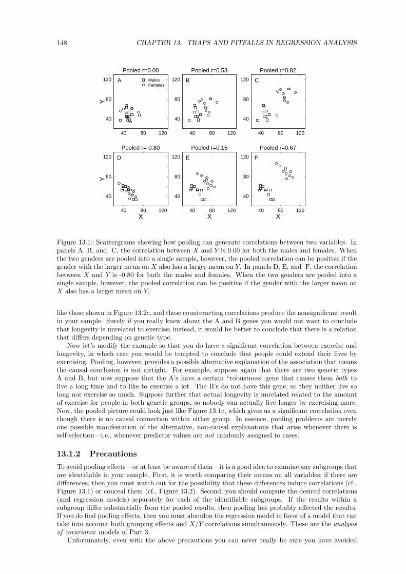
148 CHAPTER 13. TRAPS AND PITFALLS IN REGRESSION ANALYSIS
40 80 120
40
80
120
Y
Pooled r=0.00
FemalesMalesA
40 80 120
40
80
120
Pooled r=0.53
B
40 80 120
40
80
120
Pooled r=0.82
C
40 80 120X
40
80
120
Y
Pooled r=-0.80
D
40 80 120X
40
80
120
Pooled r=0.15
E
40 80 120X
40
80
120
Pooled r=0.67
F
Figure 13.1: Scattergrams showing how pooling can generate correlations between two variables. Inpanels A, B, and C, the correlation between X and Y is 0.00 for both the males and females. Whenthe two genders are pooled into a single sample, however, the pooled correlation can be positive if thegender with the larger mean on X also has a larger mean on Y. In panels D, E, and F, the correlationbetween X and Y is -0.80 for both the males and females. When the two genders are pooled into asingle sample, however, the pooled correlation can be positive if the gender with the larger mean onX also has a larger mean on Y.
like those shown in Figure 13.2c, and these counteracting correlations produce the nonsignificant resultin your sample. Surely if you really knew about the A and B genes you would not want to concludethat longevity is unrelated to exercise; instead, it would be better to conclude that there is a relationthat differs depending on genetic type.
Now let’s modify the example so that you do have a significant correlation between exercise andlongevity, in which case you would be tempted to conclude that people could extend their lives byexercising. Pooling, however, provides a possible alternative explanation of the association that meansthe causal conclusion is not airtight. For example, suppose again that there are two genetic typesA and B, but now suppose that the A’s have a certain “robustness’ gene that causes them both tolive a long time and to like to exercise a lot. The B’s do not have this gene, so they neither live solong nor exercise so much. Suppose further that actual longevity is unrelated related to the amountof exercise for people in both genetic groups, so nobody can actually live longer by exercising more.Now, the pooled picture could look just like Figure 13.1c, which gives us a significant correlation eventhough there is no causal connection within either group. In essence, pooling problems are merelyone possible manifestation of the alternative, non-causal explanations that arise whenever there isself-selection—i.e., whenever predictor values are not randomly assigned to cases.
13.1.2 Precautions
To avoid pooling effects—or at least be aware of them—it is a good idea to examine any subgroups thatare identifiable in your sample. First, it is worth comparing their means on all variables; if there aredifferences, then you must watch out for the possibility that these differences induce correlations (cf.,Figure 13.1) or conceal them (cf., Figure 13.2). Second, you should compute the desired correlations(and regression models) separately for each of the identifiable subgroups. If the results within asubgroup differ substantially from the pooled results, then pooling has probably affected the results.If you do find pooling effects, then you must abandon the regression model in favor of a model that cantake into account both grouping effects and X/Y correlations simultaneously. These are the analysisof covariance models of Part 3.
Unfortunately, even with the above precautions you can never really be sure you have avoided

13.2. RANGE RESTRICTION REDUCES CORRELATIONS 149
40 80 120X
40
80
120
Y
Pooled r=0.38
FemalesMalesA
40 80 120X
40
80
120
Pooled r=0.38
B
40 80 120X
40
80
120
Pooled r=0.00
C
Figure 13.2: Scattergrams showing how pooling can conceal correlations between two variables. Inpanels A and B, the correlation between X and Y is 0.90 for both the males and females, but thecorrelation is greatly reduced in the pooled sample. In each panel, the males and females differ ononly one variable: They differ in mean X in panel A, and they differ in mean Y in panel B. In panel Cthe correlation between X and Y is 0.80 for the males and -0.80 for the females, and it is zero for thepooled samples.
pooling effects. The danger is that your data set contains some groups that you are not aware of.You cannot look at them separately if you are not aware of them, so your overall results may becontaminated by pooling across them.
13.2 Range Restriction Reduces Correlations
Another practical issue in regression concerns the ranges of X and Y within the sample. If the rangeof either variable is somehow restricted by the sampling process, the correlation between the variableswill tend to be reduced.
The standard example of this effect concerns the correlation between IQ and grades in school, whichhas often been observed to decrease for more advanced students (e.g., high-school students versusuniversity students versus graduate students). The reason for this effect is illustrated in Figure 13.3.A sample of high-school students will include just about the full range of abilities, as shown in panel A,because almost everyone goes to high school. A sample of university students will include a narrowerrange of abilities, as shown in panel B, because the least able students tend not to go on to college.Comparing panels A and B, it is visually clear that the sample is more elongated in panel A, and thiselongation translates into a stronger correlation (r = 0.70 versus r = 0.50). The range restriction iseven more severe when the sample is restricted to graduate students, as shown in panel C, becausenow the sample will tend to include an even more restricted range of abilities. Correspondingly, thesample is less elongated and the correlation is smaller (r = 0.19).
75 100 125IQ
20
40
60
80
Gra
de
r=0.70
A
75 100 125IQ
20
40
60
80r=0.50
B
75 100 125IQ
20
40
60
80r=0.19
C
Figure 13.3: Scattergrams showing the effect of range restriction on correlation. Panel A shows therelation between IQ and grades for a sample reflecting the full range of abilities across the population.Panel B shows a subset of the data—just the subsample with IQ in the top 70%, and panel C showsjust the subsample with IQ in the top 30%. Note that the correlation decreases as the IQ rangedecreases.

150 CHAPTER 13. TRAPS AND PITFALLS IN REGRESSION ANALYSIS
13.2.1 Implications for Interpretation
As shown in Figure 13.3, range restriction tends to reduce correlations. Thus, it implies that thecorrelation in a sample might be much weaker than the true correlation in the whole population.Obviously, this is most important when you have found a nonsignificant correlation in your sample.Of course the correlation might be nonsignificant because the two variables are truly not very stronglyrelated, as you would tend to conclude. However, range restriction might have been responsible forthe absence of correlation. When examining a nonsignificant correlation, then, it is always a good ideato consider whether the sample contained the full population range on the apparently uncorrelatedvariables.
13.2.2 Precautions
The best time to take precautions against range restriction is when collecting the sample. Rangerestriction can be a very real problem with many sorts of “convenient” samples that are commonlytaken instead of random ones. For example, a sample of college students is likely to be very homogeneouswith respect to many variables (e.g., age, IQ, socioeconomic status), and it would therefore be a poorchoice for examining correlations among such variables.
It is best to avoid range restriction by selecting a truly random sample; with a truly randomsample, the likelihood of range restriction is small enough to ignore. Even if a true random sampleis impractical, you should still try to obtain a sample containing the full range of variation on thevariables you are measuring. And if there is normative data on the ranges of your variables acrossthe whole population, you should compare the range in your sample with the range in the populationto make sure that you have succeeded in sampling across the full range. The range of IQs in thenormal adult population, for example, might be 70–130, depending on the IQ test. If you measuredIQs in your sample, you would want to find that your sample covered approximately this same range,or else be prepared to face the consequences of range restriction. Finally, if you cannot avoid rangerestriction in your sample, you may still be able to correct for it after the fact using certain formulasbeyond the scope of this book. These formulas must be used with extreme caution, however, as theyare only valid if certain strong assumptions are satisfied.
13.3 Effects of Measurement Error
Many variables can be measured exactly, such as height, weight, age, income, number of children, andso on. Other variables cannot. For example, an IQ test measures IQ with some random error, partlydue to the test itself (e.g., exactly which version of the test was used) and partly due to the state ofthe person taking the test (e.g., how much sleep they had).
0 30 60 90 120X
0
30
60
90
120
Y
r=1.00
A Y=0.00+1.00 X
0 30 60 90 120X
0
30
60
90
120
r=0.45
B Y=0.00+1.00 X
0 30 60 90 120X
0
30
60
90
120
r=0.45
C Y=40.00+0.20 X
Figure 13.4: Scattergrams showing the effect of measurement errors on correlation and regression.Panel A shows a sample with a perfect X-Y correlation in a situation where both X and Y can bemeasured without error. Panel B shows the same sample, except that a random number has beenadded to each value of Y to simulate errors in measuring Y . Panel C shows the same sample, exceptthat a random number has been added to each value of X to simulate errors in measuring X . Notethat (1) errors in measuring either X or Y tend to reduce the correlation, and (2) errors in measuringX alter the slope and intercept of the regression equation, but errors in measuring Y do not.
As illustrated in Figure 13.4 and summarized in Table 13.1, measurement error can have dramatic
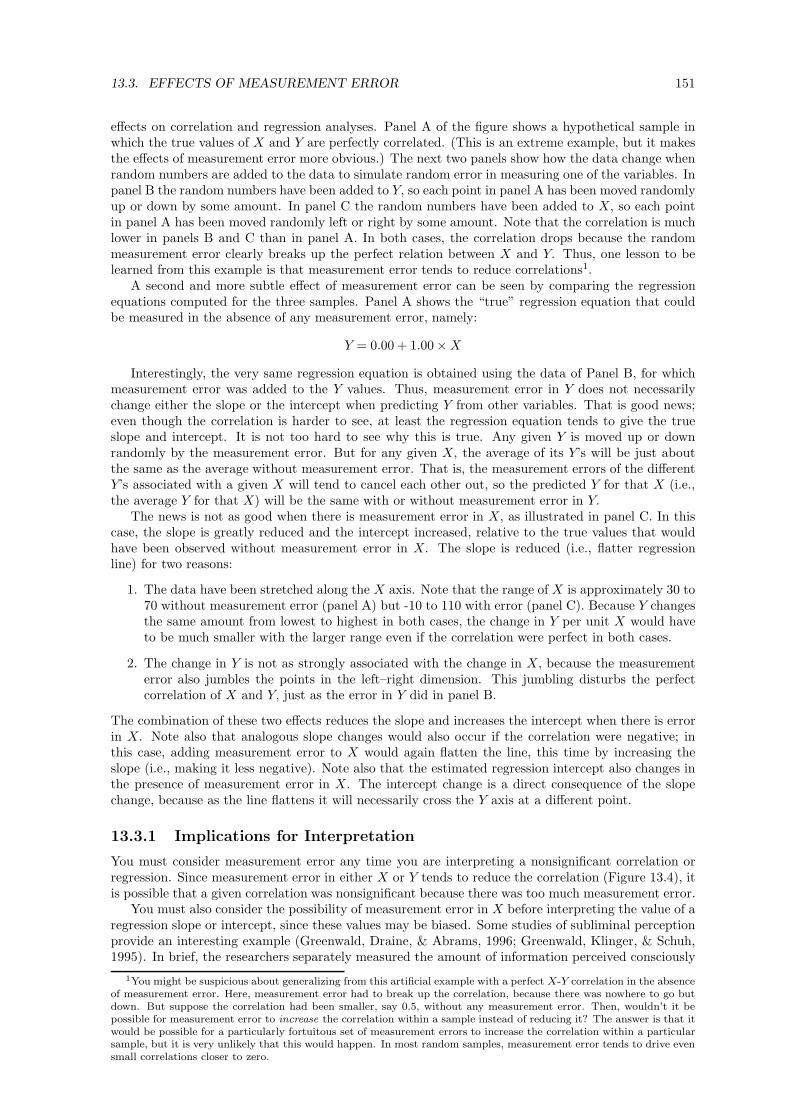
13.3. EFFECTS OF MEASUREMENT ERROR 151
effects on correlation and regression analyses. Panel A of the figure shows a hypothetical sample inwhich the true values of X and Y are perfectly correlated. (This is an extreme example, but it makesthe effects of measurement error more obvious.) The next two panels show how the data change whenrandom numbers are added to the data to simulate random error in measuring one of the variables. Inpanel B the random numbers have been added to Y, so each point in panel A has been moved randomlyup or down by some amount. In panel C the random numbers have been added to X, so each pointin panel A has been moved randomly left or right by some amount. Note that the correlation is muchlower in panels B and C than in panel A. In both cases, the correlation drops because the randommeasurement error clearly breaks up the perfect relation between X and Y. Thus, one lesson to belearned from this example is that measurement error tends to reduce correlations1.
A second and more subtle effect of measurement error can be seen by comparing the regressionequations computed for the three samples. Panel A shows the “true” regression equation that couldbe measured in the absence of any measurement error, namely:
Y = 0.00 + 1.00 × X
Interestingly, the very same regression equation is obtained using the data of Panel B, for whichmeasurement error was added to the Y values. Thus, measurement error in Y does not necessarilychange either the slope or the intercept when predicting Y from other variables. That is good news;even though the correlation is harder to see, at least the regression equation tends to give the trueslope and intercept. It is not too hard to see why this is true. Any given Y is moved up or downrandomly by the measurement error. But for any given X, the average of its Y’s will be just aboutthe same as the average without measurement error. That is, the measurement errors of the differentY’s associated with a given X will tend to cancel each other out, so the predicted Y for that X (i.e.,the average Y for that X) will be the same with or without measurement error in Y.
The news is not as good when there is measurement error in X, as illustrated in panel C. In thiscase, the slope is greatly reduced and the intercept increased, relative to the true values that wouldhave been observed without measurement error in X. The slope is reduced (i.e., flatter regressionline) for two reasons:
1. The data have been stretched along the X axis. Note that the range of X is approximately 30 to70 without measurement error (panel A) but -10 to 110 with error (panel C). Because Y changesthe same amount from lowest to highest in both cases, the change in Y per unit X would haveto be much smaller with the larger range even if the correlation were perfect in both cases.
2. The change in Y is not as strongly associated with the change in X, because the measurementerror also jumbles the points in the left–right dimension. This jumbling disturbs the perfectcorrelation of X and Y, just as the error in Y did in panel B.
The combination of these two effects reduces the slope and increases the intercept when there is errorin X. Note also that analogous slope changes would also occur if the correlation were negative; inthis case, adding measurement error to X would again flatten the line, this time by increasing theslope (i.e., making it less negative). Note also that the estimated regression intercept also changes inthe presence of measurement error in X. The intercept change is a direct consequence of the slopechange, because as the line flattens it will necessarily cross the Y axis at a different point.
13.3.1 Implications for Interpretation
You must consider measurement error any time you are interpreting a nonsignificant correlation orregression. Since measurement error in either X or Y tends to reduce the correlation (Figure 13.4), itis possible that a given correlation was nonsignificant because there was too much measurement error.
You must also consider the possibility of measurement error in X before interpreting the value of aregression slope or intercept, since these values may be biased. Some studies of subliminal perceptionprovide an interesting example (Greenwald, Draine, & Abrams, 1996; Greenwald, Klinger, & Schuh,1995). In brief, the researchers separately measured the amount of information perceived consciously
1You might be suspicious about generalizing from this artificial example with a perfect X-Y correlation in the absenceof measurement error. Here, measurement error had to break up the correlation, because there was nowhere to go butdown. But suppose the correlation had been smaller, say 0.5, without any measurement error. Then, wouldn’t it bepossible for measurement error to increase the correlation within a sample instead of reducing it? The answer is that itwould be possible for a particularly fortuitous set of measurement errors to increase the correlation within a particularsample, but it is very unlikely that this would happen. In most random samples, measurement error tends to drive evensmall correlations closer to zero.

152 CHAPTER 13. TRAPS AND PITFALLS IN REGRESSION ANALYSIS
Measurement Error inEffect on: X YCorrelation Reduces r. Reduces r.
Slope Slope flattened. No systematic effect.
Intercept Intercept biased because No systematic effect.of change in slope.
Table 13.1: Effects of Measurement Error on Correlation and Regression Analysis
(X) and unconsciously (Y), and then computed a regression to predict Y from X. The crucial findingwas that the intercept was greater than zero, which they interpreted as evidence some informationwas perceived unconsciously even when none was perceived consciously (i.e., Y greater than zero whenX=0). Others have questioned their methodology, however, because their measure of X was subjectto some measurement error, and this error would have biased the intercept to be greater than zero(Dosher, 1998; Miller, 2000).
13.3.2 Precautions
The obvious precaution is to eliminate measurement error, especially error in X if a regression equationis to be computed. While this is easy enough to recommend within the pristine confines of a statisticstext, it is often impossible to achieve in the messy real world of data collection. In situations wheremeasurement error is unavoidable, the only hope is to measure it and to estimate its probable effectson the correlation and regression analyses. Techniques for accomplishing this are beyond the scope ofthis book, however.
A final comment about measurement error is that in regression analysis, unlike ANOVA, it cannotbe completely overcome by increasing the sample size. In ANOVA, random error tends to averageout as sample size increases, so the observed pattern of cell means approaches the true pattern assample size increases. Measurement error does not distort the pattern of means, but merely increasesthe sample size needed to approach the true pattern. In regression, though, measurement error doesnot magically go away as the sample size is increased. Consider, for example, the difference betweenpanels A and B of Figure 13.4. The data patterns differ because of the measurement error in Y, andthe difference will persist no matter how large a sample is included in panel B.
13.4 Applying the Model to New Cases
In some situations it is desirable to use the results of a regression analysis to make predictions fornew cases. This is a type of extrapolation, because the model was developed on one set of cases andthen is being used to make predictions about a new set. It is natural to wonder how accurate yourpredictions will be when you extrapolate like this. As an example, suppose you developed a modelto predict the outcomes of horse races, intending to use the model to guide your bets and win somemoney. To develop the model, you would collect a data set with a to-be-predicted variable (e.g., eachhorse’s finishing time) and one or more predictor variables. You would then fit a regression modelto predict Y from the X’s, and if the model fit well you would use it to predict the outcomes of newraces on which you intended to bet. How accurate would you expect these predictions to be?
It seems natural to expect that the errors in your new predictions would be about the same as theestimated errors (ei = Yi −Y ′
i ) that you computed for your sample. If the MSerror in your regressionanalysis were 100, for example, you might expect the average prediction error to be approximatelythe square root of that—around 10. Unfortunately, this expectation is too optimistic, and your realaverage error would very likely be greater than 10.
Why does error tend to increase when making predictions for new cases? The main reason is thesampling error in the regression slope and intercept values. The key point is that a and b are theoptimal values leading to the minimum MSerror for the original sample, not for the population as awhole. When you use the sample values to make predictions about the new cases, then, you are notreally using the best values—the true population values would be better. The prediction error for newcases will be inflated as a result.
To illustrate this increase in prediction error when extrapolating to new cases, consider a simplehypothetical situation in which samples are taken from a known population. Imagine that the

13.5. REGRESSION TOWARDS THE MEAN 153
scattergram shown in panel A of Figure 13.5 represents the X and Y values for an entire population of250 individuals, perhaps animals of some endangered species. As indicated in the panel, the optimalregression line for this population is Yi = 85.0 + 0.300 × Xi.
0 20 40 60 80 100X
75
90
105
120
135
Y
Population
A Y=85.0+0.300 X
0 20 40 60 80 100X
75
90
105
120
135
Sample
B Y=82.4+0.347 X
Figure 13.5: Scattergrams to illustrate why prediction error tends to increase when predictions aremade for new cases. Panel A shows the relation between X and Y for a full population of 250 cases;panel B shows the relation for a random sample of 25 cases from this population.
Now imagine that you have only a random sample of 25 of these cases, shown in panel B, asyou might get in a real research situation. From these cases you compute the regression line Yi =82.4 + 0.347 × Xi. Note that the sample’s slope and intercept differ from their true populationvalues; this is, of course, because of sampling error. Furthermore, this regression analysis yieldsMSerror = 61.196, which might lead you to expect a typical prediction error to be approximately√
61.196 = 7.82 when making predictions for new cases. But if you apply this predictive model to theremaining 225 “new” cases in the population, you’ll get a value of
√65.612 = 8.10 as the resulting
average error.2 Thus, a typical prediction error when making predictions for new cases is about 3.5%larger than you would have guessed from looking at the analysis of the random sample.
You might think that you could avoid this problem by including each new case in the sample andrefitting the model every time a new data value is obtained. Note, however, that you need both Xand Y for the new case in order to refit the model including this case. But if you wait to have bothX and Y, then it is too late to act on your predicted Y value. In the case of betting on horse races,for example, you must place your bet before the finishing time (Y) is determined—that is, before it ispossible to refit the model including that case.
13.4.1 Implications for Interpretation
The only implication is the obvious one: that prediction error should be expected to be somewhatlarger for new cases than for the sample itself.
13.4.2 Precautions
There is no way to avoid the increase in prediction error, so the only possible precaution is to estimateit and allow for it. The technical issue of how much increase in prediction error to expect is beyondthe scope of this book. Two qualitative points will suffice for our purposes:
• Prediction error increases more if the model has more predictors.
• Prediction error increases less if the model is based on a larger sample.
13.5 Regression Towards the Mean
Regression towards the mean (also known as “regression to the mean” or “statistical regression”) isa reasonably simple concept, but its applications are often difficult to spot. This section will explainthe basic concept, and the next section on “Implications for Interpretation” will explain why you needto know about it.
In brief, “regression towards the mean” is simply a name for this fact:
2To be more specific, for each of the other 225 cases I computed ei = Yi − 82.4 + 0.347 × Xi. 65.612 is the averageof the 225 squared ei values.

154 CHAPTER 13. TRAPS AND PITFALLS IN REGRESSION ANALYSIS
When you make a prediction with a regression model, the predicted value will be closerto its mean than the predictor is to its mean.
That is, Y ′
i is closer to Y than Xi is to X, (ignoring a few mathematical loose ends that will be dealtwith shortly).
Panel A of Figure 13.6 provides an illustrative data set. The to-be-predicted variable is the heightof a son, and the predictor variable is the father’s height. These are fictitious data, but they are prettyrealistic except that for convenience the fathers and sons have identical mean heights (180 cm) andstandard deviations of height (10 cm).
160 180 200Father’s Ht
160
180
200
Son
’sH
t
A
Son’=44.8+0.75 Father
160 180 200Father’s Ht
160
180
200B
160 180 200Father’s Ht
160
180
200C
Figure 13.6: Panel A shows a scattergram of 500 cases showing the relationship between heights offathers and heights of their sons. The best-fitting regression line and its equation are shown on thegraph. Panels B and C show the same scattergram with certain groups of cases indicated by dashedlines, as discussed in the text.
The best-fitting regression line to predict son’s height from father’s height, shown on the graph,is Son′ = 44.8 + 0.75 × Father. Table 13.2 shows some example predictions computed using thisequation. Note that for each case in this table the value of Y ′
i is closer to the mean 180 than is Xi.That is, for small values of Xi, Y ′
i is larger than Xi, whereas for large values of Xi, Y ′
i is smaller thanXi. This is simply the phenomenon of regression towards the mean as it applies to these cases.
Father’s Height (Xi) Predicted Son’s Height Y ′
i
150 44.8 + 0.75 × 150 = 157.3160 44.8 + 0.75 × 160 = 164.8170 44.8 + 0.75 × 170 = 172.3190 44.8 + 0.75 × 190 = 187.3200 44.8 + 0.75 × 200 = 194.8210 44.8 + 0.75 × 210 = 202.3
Table 13.2: Example predicted values using regression equation to predict son’s height from father’sheight.
The regression toward the mean illustrated in Table 13.2 is not just an accident of this particulardata set, but it reflects a phenomenon that holds across all possible data sets. One relevant equationis this: ∣∣∣∣
Y ′
i − Y
sy
∣∣∣∣ = |rxy| ×∣∣∣∣Xi − X
sx
∣∣∣∣ (13.1)
In words, it says that the absolute distance from the predicted Y ′
i to Y (measured relative to thestandard deviation of the Y scores) is equal to the absolute value of the sample correlation coefficienttimes the absolute distance from the predictor value Xi to X (measured relative to the standarddeviation of the X scores). Since the absolute value of the correlation is virtually always less than1.0, it follows that Y ′
i is virtually always closer to Y than Xi is to X , with distances on both variablesmeasured relative to their respective standard deviations.
Intuitively, one way to explain this is as follows: If you have no information on which to basea prediction, your best strategy is to guess the mean of the variable you are trying to predict. Forexample, if you had to guess a son’s height without knowing anything at all, your best guess wouldbe the mean height, 180 cm. Now if you get some useful predictive information, such as the father’sheight, this causes you to move your prediction away from the mean. For example, if the father’s

13.5. REGRESSION TOWARDS THE MEAN 155
height is one standard deviation above average, then we would expect the son’s height to be aboveaverage too. But how much above average? Not a full standard deviation, as the father’s height was,because father’s and son’s heights are only imperfectly correlated. In fact, if the correlation is onlyrxy = 0.5, then you should expect the son’s height to be one-half a standard deviation above average.
It is important to realize that regression toward the mean is actually a common phenomenon inthe real world, not just an abstract mathematical property of this particular statistical model. Thatis, the regression model is “right” to keep its predictions relatively close to the mean Y, because thesepredictions will be most accurate in the long run. For example, tall fathers really do tend to havesomewhat shorter sons, on average, and very short fathers really do tend to have somewhat tallersons. This is part of what makes regression models appropriate and useful in real-world situations.
This property is inherent in all normally distributed populations, and it was first observed byFrancis Galton in an analysis of the genetic transmission of height in the 1880s, around the time ofDarwin’s then-new genetic theory. The basic data set was a collection of father’s and son’s heights,as we have been considering (e.g., Figure 13.6). Regression analysis had not yet been invented yet,so the investigators used their data to construct a table like that shown in Table 13.3. First, caseswere grouped according to the heights of the fathers. For example, one group contained all the caseswith fathers heights in the range from 150–160 cm. Second, each group of cases was summarized bycomputing the average height of the fathers in that group and the average height of the sons in thatgroup.
Father’s Height Number Average Height Average HeightGroup Range for Group of Cases of Fathers of Sons
1 150–160 11 156.0 166.62 160–170 61 165.3 169.23 170–180 163 174.9 175.44 180–190 182 184.2 183.15 190–200 73 193.5 191.26 200–210 10 203.5 196.4
Total 150–210 500 180.0 180.0
Table 13.3: A summary tabulation of the cases shown in Figure 13.6. Each case was assigned toone group depending on the height of the father. After the groups had been determined, the averageheights of fathers and sons in each group were determined.
The results shown in Table 13.3 are representative of what was actually obtained, and they illustrateclear regression toward the mean. For example, the fathers with heights in the 150–160 cm rangetended to have somewhat taller sons, with an average height of 166.6 cm. Similarly, the fathers withheights in the 200–210 cm range tended to have somewhat shorter sons, with an average height of196.4 cm. For each group, the average of the son’s heights is closer to the overall mean height (180 cm)than the average height of the fathers in that group.
As an historical aside, inspection of data like that shown in Table 13.3 initially led scientists toconclude that something about the mechanisms of genetic transmission worked to even out heightsacross many generations. They apparently believed that individual differences in height had beengreater in the past, were diminishing with successive generations, and would eventually all butdisappear. In fact, the term “regression” originated within statistics in precisely this context, todescribe this pattern of apparent change over time.
It was not long before these researchers realized that the pattern of regression shown in Table 13.3resulted from some sort of statistical effect rather than genetic mechanisms. This was discovered whensomeone decided to have another look at the same data, this time grouping the cases according tothe sons’ heights instead of the fathers’. The new tabulation yielded a pattern like the one shown inTable 13.4.
Contrary to genetic explanations of the regression (and to most people’s intuitions at this point!),the exact opposite pattern of regression was obtained when the cases were grouped according to thesons instead of the fathers. As you can see, for every group in Table 13.4, the average height of thefathers is closer to the mean than the average height of the sons. That is, the fathers’ heights regresstoward the mean, not the sons heights. This suggests that heights are getting more extreme from onegeneration to the next, not less extreme as suggested by the tabulation in Table 13.3. How can thesame data lead to two opposite conclusions?

156 CHAPTER 13. TRAPS AND PITFALLS IN REGRESSION ANALYSIS
Son’s Height Number Average Height Average HeightGroup Range for Group of Cases of Fathers of Sons
1 150–160 5 161.2 157.42 160–170 71 169.7 165.93 170–180 175 175.9 174.74 180–190 163 183.6 184.45 190–200 68 189.7 193.26 200–210 17 195.5 202.47 210–220 1 208.0 213.0
Total 150–210 500 180.0 180.0
Table 13.4: A summary tabulation of the cases shown in Figure 13.6. Each case was assigned to onegroup depending on the height of the son. After the groups had been determined, the average heightsof fathers and sons in each group were determined.
The answer is that in both tables the regression towards the mean results from grouping thebivariate distribution:
When cases are grouped according to one variable, the group averages on a secondvariable tend to be less extreme than the group averages on the first (grouping) variable.
First, look back at Tables 13.3 and 13.4 to see that this is an accurate summary. Next, look backat panels B and C of Figure 13.6 to see why this is true. Panel B illustrates grouping accordingto fathers’ heights. The two columns set off by vertical dashes correspond to the cases in which thefathers’ heights were in the ranges of 150–160 cm and 200–210 cm. If you examine the points capturedin the left-most column (i.e., fathers heights of 150–160 cm), you can see that the average height of thesons in this group is clearly more than 160 cm. Because of the scattergram’s cloud shape (i.e., becausethe two variables have normal distributions), many of the cases with very low values on father’s heighthave not-so-low values on son’s height, and these points bring up the average sons’ height for thatgroup. Similarly, if you examine the points captured in the right-most column (i.e., fathers heights of200–210 cm), you can see that the average height of the sons in this group is clearly less than 200 cm.Again because of the scattergram’s cloud shape, many of the cases with very high values on father’sheight have not-so-high values on son’s height, and these points bring down the average sons’ heightfor that group. To summarize, when you select out the extreme fathers, their sons tend to be moretoward the middle of the cloud because that is where most of the points are.
Panel C illustrates the same point, now grouping according to sons’ heights instead of fathersheights. The two rows set off by horizontal dashes correspond to the cases in which the sons’ heightswere in the ranges of 150–160 cm and 200–210 cm. If you examine the points captured in the lowerrow (i.e., sons heights of 150–160 cm), you can see that the average height of the fathers in this groupis clearly more than 160 cm. Again, this is because of the scattergram’s cloud shape. Similarly, if youexamine the points captured in the upper row (i.e., sons heights of 200–210 cm), you can see that theaverage height of the fathers in this group is clearly less than 200 cm. Likewise, then, when you selectout extreme sons, their fathers tend to be more toward the middle of the cloud because that is wheremost of the points are.
One final but important point about regression toward the mean is that it only applies on theaverage, not necessarily for every case. In the data set shown in Figure 13.6, for example, there was afather in the tallest group (208 cm) who had an even taller son (213 cm). Similarly, there was a sonin the tallest group (204 cm) who had an even taller father (208 cm). Obviously, regression towardthe mean did not operate in these two individual cases. With normal distributions, though, it mustoperate on the average across large numbers of cases.
13.5.1 Implications for Interpretation
The phenomenon of regression toward the mean must be kept in mind whenever cases are groupedor selected using one (or more) variables and then tested or measured on a different variable. Youhave to keep in mind that the pattern observed on the measured variable might be due to a purelystatistical phenomenon: regression toward the mean.
For example, assume that the following was demonstrated: “Women who go to University tend tomarry men who are less intelligent than they are.” You can imagine a variety of causal explanations

13.5. REGRESSION TOWARDS THE MEAN 157
of this that you might read in a newspaper or magazine: For example, someone might argue fromthis observation that University somehow makes women less desirable marriage partners and so theyhave less intelligent suitors than they would have had otherwise. Before entertaining any such causalexplanation, however, you must first realize that this phenomenon could simply be another exampleof regression toward the mean. Suppose we consider married couples to be cases. We now select outa group in which the IQs of the wives are higher than 110 (the wives must have relatively high IQs,because they went to University), and measure the group average IQ of the husbands. Naturally itwill be lower than the wive’s average, just due to the phenomenon of regression toward the mean. Thesituation is depicted in Figure 13.7, which is analogous to Figure 13.6. Critically, there is no basis toconclude that going to University has any causal influence on its own. There may be such influences,but this effect doesn’t demonstrate them because the effect can be explained entirely by regressiontoward the mean. (And of course the converse should also be true—University men should tend tomarry women who are less intelligent, on average, than they are—for exactly the same reason.)
40 60 80 100120140160Wife’s IQ
40
60
80
100
120
140
160
Hus
band
’sIQ
A
40 60 80 100120140160Wife’s IQ
40
60
80
100
120
140
160B
Figure 13.7: Panel A shows a scattergram of 300 cases showing the relationship between IQs of wivesand husbands. Panel B shows the same scattergram with the wives who attended University indicatedby dashed lines, as discussed in the text. The mean IQ of these wives is 119, whereas the mean IQ oftheir husbands is 113. This diagram is an oversimplification of the true situation, because in realitythere is no absolute cutoff IQ separating women who do and do not attend University. Despite thisoversimplification, the diagram illustrates why the mean IQ of the wives would likely be greater thanthe mean IQ of their husbands.
Another classic example is that people are often disappointed when they go back for a secondmeal at a restaurant where they had particularly wonderful food on their first visit. Whether theyorder the same dish or a new one on that second trip, they will often find that the food just isn’tas pleasing as it was before. This is to be expected on the basis of regression toward the mean. Inthis example, the restaurant is the case, and your subjective impressions of the first and second mealsare the two variables. When you select out the subset of restaurants with really good scores on thefirst meal, the average of the second meal impressions is bound to be lower. You would notice theanalogous phenomenon if you selected restaurants where the second meal was especially outstanding(i.e., the first meals would not have been as good, on average), but this is not as salient a comparisonpsychologically.
As a third and slightly more complicated example, suppose you are evaluating two new Universityprograms designed to meet the needs of special students. One program is aimed at high achievers.Students are invited to join after they achieve (say) an average of at least 85% across all their coursesfor one semester. Once they are in the program, they are invited to special lectures and Universityfunctions designed to help them develop their potential to the fullest. The other program is aimed atunderachievers. Students are invited to join this one if they score less than 60% in a semester, andthey are given special tutoring and remedial help. At the end of one semester, the results come back.Disappointingly, in the “high achievers” program, the students’ average has dropped from 87% beforethe program to 83% in it. The other program is apparently going much better, however, because theunderachievers raised their averages from 56% to 63%. Naturally, you are tempted to conclude thatthe high achievers program is at best useless—possibly harmful (e.g., too distracting)—and should bescrapped. In contrast, the underachievers program is producing big gains. Obviously, you should putall your efforts into the underachievers program, right?
Wrong. Students were selected into groups (“high achievers” versus “underachievers”) based onscores in one semester, and then their performance was assessed based on new scores from anothersemester. The phenomenon of regression toward the mean dictates that, on average, the high scores

158 CHAPTER 13. TRAPS AND PITFALLS IN REGRESSION ANALYSIS
must decrease and the low scores must increase. That is exactly what happened! Based on theseresults, you can’t say for sure that either program did anything at all, because regression toward themean provides a perfectly good explanation of the results all by itself. It could be that one or bothprograms are useful, of course, and in fact the high achievers program could even be the better one.You just can’t tell from the information you have at hand.
13.5.2 Precautions
Regression toward the mean is a real statistical phenomenon, present whenever variables are normallyor near-normally distributed. There is no way to eliminate it, so you must be aware of it. If youconsider it when designing a study, you may be able to control for its effects, as discussed next. Evenif you don’t consider it until the data are in, you can at least avoid making conclusions that are invalidbecause it might be operating.
In many situations, the effects of regression toward the mean can be determined by including acontrol group. Then, you can see if the experimental effects are larger than those in the control group;if so, you can dispense with regression toward the mean as an explanation.
As an example, consider again evaluating the programs for high achievers and underachievers.Instead of inviting all qualified students into the two programs, you would be better off to invite onlya randomly selected half of each group into each program. The other, uninvited halves could be heldout of the program for a semester to serve as control groups, and changes in their scores would includethe effects of regression toward the mean (as well as seasonal effects, etc). At the end of one semester,you would have data for these four groups:
High Achievers Program Underachievers ProgramIn Program Control In Program Control
1 2 3 4
You could legitimately compare groups 1 and 2 to evaluate the high achievers program. Because ofregression toward the mean, you would expect both these groups to have somewhat lower averagescores in this semester than in the previous one. If the program is helpful, though, the dip shouldbe smaller for the students who were in it. Similarly, you could compare groups 3 and 4 to evaluatethe underachievers program. Both groups should increase relative to the previous semester due toregression towards the mean. If the program is helpful, though, group 3 should show a larger increasethan group 4.

Chapter 14
Multiple Regression
14.1 Introduction
A multiple regression model is used to quantify the relationship of a Y variable and two or more Xvariables. Just as in simple regression, the purposes of quantifying the relationship are (a) prediction,and (b) looking for signs of causal relationships.
A multiple regression model is used with data in the “Case by Variable” format, an example ofwhich is shown in Table 14.1. As in simple regression, there is a single sample of cases, and each caseis measured with respect to a numerical Y variable. In multiple regression, each case is also measuredwith respect to two or more X variables.
Case PERF TRA EXP IQ Predicted Error1 62 13 15 85 60.49 = -22.61 + 2.37 × 13 + 1.60 × 15 + 0.33 × 85 1.51 = 62 - 60.492 67 11 14 123 66.76 = -22.61 + 2.37 × 11 + 1.60 × 14 + 0.33 × 123 0.24 = 67 - 66.763 73 12 13 127 68.86 = -22.61 + 2.37 × 12 + 1.60 × 13 + 0.33 × 127 4.14 = 73 - 68.864 75 11 20 120 75.39 = -22.61 + 2.37 × 11 + 1.60 × 20 + 0.33 × 120 -0.39 = 75 - 75.395 54 7 19 99 57.33 = -22.61 + 2.37 × 7 + 1.60 × 19 + 0.33 × 99 -3.33 = 54 - 57.336 69 10 13 114 59.80 = -22.61 + 2.37 × 10 + 1.60 × 13 + 0.33 × 114 9.20 = 69 - 59.807 64 12 15 124 71.07 = -22.61 + 2.37 × 12 + 1.60 × 15 + 0.33 × 124 -7.07 = 64 - 71.078 59 10 10 124 58.31 = -22.61 + 2.37 × 10 + 1.60 × 10 + 0.33 × 124 0.69 = 59 - 58.319 57 12 13 99 59.56 = -22.61 + 2.37 × 12 + 1.60 × 13 + 0.33 × 99 -2.56 = 57 - 59.56
10 49 10 12 80 46.91 = -22.61 + 2.37 × 10 + 1.60 × 12 + 0.33 × 80 2.09 = 49 - 46.9111 55 8 11 113 51.52 = -22.61 + 2.37 × 8 + 1.60 × 11 + 0.33 × 113 3.48 = 55 - 51.5212 42 8 11 112 51.19 = -22.61 + 2.37 × 8 + 1.60 × 11 + 0.33 × 112 -9.19 = 42 - 51.1913 63 8 18 107 60.76 = -22.61 + 2.37 × 8 + 1.60 × 18 + 0.33 × 10⁷ 2.24 = 63 - 60.7614 60 7 15 116 56.56 = -22.61 + 2.37 × 7 + 1.60 × 15 + 0.33 × 116 3.44 = 60 - 56.5615 50 10 11 107 54.27 = -22.61 + 2.37 × 10 + 1.60 × 11 + 0.33 × 10⁷ -4.27 = 50 - 54.27
Sum: 899 899.00 0.00Mean: 59.93 59.93 0.00
SumSq: 55049 54740.62 308.38
Table 14.1: Hypothetical example data set for multiple regression. The researcher is interested infinding out how on-the-job performance (PERF) by computer operators is related to weeks of training(TRA), months of experience (EXP), and IQ. The right-most two columns (“Predicted” and “Error”)are not part of the data set but emerge in doing the computations, as described below.
14.2 The Model for Multiple Regression
All multiple regression models have this form:
Yi = a + b1 × X1i + b2 × X2i + ei
The Yi values in the model are the observed values of the to-be-predicted variable, analogous tothe dependent variable in ANOVA. For the example in Table 14.1, the Yi values are the PERF scores.The subscript i is used to distinguish the different cases; for example, Y13 is 63.
The a term in the model is a constant, analogous to a baseline in ANOVA. As in simple regression,it is rarely of much interest in multiple regression but it must nonetheless be included in the modelfor computational reasons.
159

160 CHAPTER 14. MULTIPLE REGRESSION
The model terms of primary interest are
• b1 × X1i
• b2 × X2i
• b3 × X3i
• and so on.
These terms capture the relationships of the X variables to Y.Each of these b × X terms involves a different one of the predictor variables X1i, X2i, etc. The
first subscript (1,2,3,. . . ) is used to differentiate among the different predictor variables, and the isubscript is used to differentiate among the cases just as it does with Yi. In Table 14.1, for example,the values of X1i are the values of the first predictor variable, namely TRA, and X1,6 is the TRAvalue for the 6th case—i.e., 10. Continuing on from left to right as is standard, X2i denotes the valuesof the EXP variable and X3i denotes the values of the IQ variable.
The terms b1, b2, b3, and so on are the “regression slopes.” Each slope captures the linearrelationship between Y and its associated predictor or X variable, just as a slope does in simpleregression. Unlike simple regression, however, each multiple regression slope should be thought of asindicating how Y would change with X if all of the other X’s were held constant. If you examine themultiple regression equation, you can see that if b1 is zero, then the term b1 × X1i is also zero, andthe first predictor variable totally drops out of the model. In other words, if X1i does not help predictYi when all of the other X’s are taken into account, then b1 will be adjusted to (nearly) zero andthe model will (essentially) ignore the value of X1i in predicting Yi. On the other hand, if the X1i
values do help predict Yi (for a constant set of other X’s), then b1 will be adjusted to an appropriatepositive or negative value. For example, if Yi tends to increase as X1i increases (with all of the otherX’s held constant), then b1 will be set to a positive value. That will mean that larger values of X1i
will produce larger predicted values of Yi, with the other X’s remaining constant.1
Thinking in ANOVA terms, each b × X term is analogous to a main effect of that X variable.In a sense, then, the regression model includes main effects. But it includes only these main effects(and error)—it does not include anything corresponding to an interaction of two or more factors. Inprinciple one could include interaction terms in regression models, but this is an advanced topic thatwe will not cover.
Finally, the ei term is the random error term in the model. As usual, the model attributes torandom error anything that it cannot explain. Also as usual, the size of the estimated random erroris used as a yardstick to decide whether other effects are “real” or “small enough that they might bedue to chance.”
14.3 A Limitation: One F per Model
There is an important limitation of the regression model that many students find puzzling at first:With a multiple regression model, you only get one F that jointly tests whether Y is related to anyof the predictors. This is very different from ANOVA, where we got one F to test each factor’s maineffect separately (and more F ’s for interactions). In contrast, with a multiple regression model youonly get one F for the whole model, regardless of the number of predictors.
The reasons for this limitation can be explained more easily after we have seen how the multipleregression model itself is used and how it can be extended with a technique called the “Extra Sumof Squares Comparison”, described in Chapter 15. In essence, though, the idea is that the differentpredictors work together in ways that are difficult to measure separately.
Perhaps an analogy to team sports will be helpful: In many team sports where the players allwork together to try to score (e.g., soccer, rugby, net ball), it is very difficult to measure the valueof each player to the team’s scoring. Obviously, just measuring the points scored by that playerwould not be a very good measure, because some players might be extremely valuable to the offenseeven if they don’t score many points. For example, a player might be exceptionally good at making“assists”—that is, at getting the ball into a position where other players on their team can score.Clearly, such a player would make a large contribution to the team’s scoring, even if he or she never
1It is tedious to keep specifying the condition “with the other X’s remaining the same” or equivalent, so henceforthwe will omit this condition, but it should always be understood to be implicitly present in the multiple regressionsituation.

14.4. COMPUTATIONS 161
personally scored any points at all, as could be demonstrated by removing the player from the teamand seeing its scores fall. It is easy to see that the possibility of such assists makes it more difficultto quantify each player’s contribution to the scoring in this type of sport. In contrast, there are othersports (e.g., cricket, baseball) where scoring is done more by individual effort, and in these sports itis correspondingly easier to measure each player’s individual contribution to the offense.
For now, suffice it to say that multiple regression is more like soccer than like cricket, so it isrelatively difficult to measure out each predictor’s separate contribution to the model; ANOVA ismore like cricket. For now, it will be enough to be aware that a multiple regression model (unlike anANOVA) does not give you a separate F to isolate the predictive contribution of each predictor. Toget information on a predictor’s separate contribution to the model requires a type of extra analysis,typically done after the multiple regression, that will be covered in Chapter 15.
14.4 Computations
Although the computations are more complex, the principles underlying the multiple regression modelare remarkably similar to those used in simple regression. As usual, you:
• Write down the model.
• Estimate the parameters of the model—namely, compute a, b1, b2, . . . .
• Compute the predicted Y value and error for each case.
• Compute sums of squares.
• Compute a summary table and test null hypotheses.
14.4.1 Estimation of a and the b’s
The main difference between multiple regression and simple regression is that you need a computerto estimate the values of a and the b’s. I will not even present the estimation equations, because theycannot be written down very compactly without using matrix algebra. For our purposes, then, it willremain mysterious how these values are computed. Note, however, that the computation leads to thebest possible values of a and the b’s. That is, the computation gives us the unique set of values thatlead to the most accurate predictions of Y for our sample. That is, if the X’s are good predictors, thea and b values will produce predicted Y’s quite close to the actual Ys. Thus, the a and b values areexactly those numbers that best capture the relationships among the variables in the current data set.
For the example data set in Table 14.1, the best values turn out to be:
a = -22.609
b1 = 2.371
b2 = 1.604
b3 = 0.332
This means that the best predictions of performance are obtained by using the following predictiveequation for PERF, which is a specific instantiation of the more general regression prediction equationwritten below it:
PERF’ = -22.609 + 2.371 × TRA + 1.604 × EXP + 0.332 × IQ
Y ′
i = a + b1 × X1i + b2 × X2i + b3 × X3i
14.4.2 Predicted Y Values
Once you have the values of a and the b’s, the prediction equation is used to compute a predicted Yvalue for each case. In general, the formula is
Y ′
i = a + b1 × X1i + b2 × X2i + . . .
Note the “prime” after the Y, which again denotes that it is a predicted value rather than an observedone. For each case, you get an overall predicted performance value like this:
1. plug in the numerical values of TRA, EXP, and IQ for that case,

162 CHAPTER 14. MULTIPLE REGRESSION
2. multiply each by its associated value of the b,
3. add these products, and
4. add in the estimated a.
For example, the “Predicted” column in Table 14.1 shows the computation of predicted values forthat data set, using the best predictive model, already given as:
PERF’ = -22.609 + 2.371 × TRA + 1.604 × EXP + 0.332 × IQ
Note that the TRA, EXP, and IQ values for each case are substituted into the right side of the formula.
14.4.3 Error Estimates
Once you have the predicted values for all cases, the next step is to compute the error scores, also caseby case. As usual, each error value is simply the number needed to set the two sides of the equationto equality. The simplest way to compute this value is with the equation:
ei = Yi − Y ′
i (14.1)
The “Error” column in Table 14.1 shows the computations of the ei values for that data set.
14.4.4 Sums of Squares
As in simple regression, four sums of squares are normally computed in connection with the regressionmodel. The computational formulas for these are:
SSµ = N × Y × Y
SSmodel =N∑
i=1
Y ′
i2 − SSµ
SSerror =
N∑
i=1
ei2
SScorrected total =
N∑
i=1
Yi2 − SSµ
Here are the specific versions of these equations for the data shown in Table 14.1:
SSµ = 15 × 59.93× 59.93 = 53880.07
SSmodel = 54740.62− 53880.07 = 860.55
SSerror = 308.38
SScorrected total = 55049.00− 53880.07 = 1168.93
The SSµ is computed in the same way as in ANOVA. In regression analysis, it is only used tocorrect other sums of squares when the mean Y is not zero. (Note: The SSµ is sometimes referred toas SSa.)
The interpretation of the SSerror is the simplest: It is a measure of the total error in prediction,across all the cases.
The SScorrected total can be interpreted as the total variation (in Y) that the model is attemptingto predict. It is perhaps illuminating to look at a more conceptually informative alternative versionof the formula for this quantity:
SScorrected total =
N∑
i=1
(Yi − Y )2 (14.2)
Note that this sum of squares will be zero if the Y values are all the same—i.e., if they do not vary.To the extent that they do vary, SScorrected total will be greater than zero, and the goal of the modelis to predict this variation in the Y’s.

14.5. INTERPRETATION & CONCLUSIONS 163
Finally, the SSmodel is a measure of the extent to which the model actually does predict theobserved variation in Y. Again, this is easiest to see when looking at a more conceptually informativealternative version of the formula:
SSmodel =
N∑
i=1
(Y ′
i − Y )2 (14.3)
Note that this sum of squares will be the same as SScorrected total if the predictions are perfect. Inthat case, the predicted Y will be equal to the observed Y for every case (that’s just what is meant byperfect predictions), and so the right sides of Equations 14.2 and 14.3 would be the same.
It is also worth noting that the easiest way to compute SSmodel is to use this equation, aftercomputing SScorrected total and SSerror:
SSmodel = SScorrected total − SSerror (14.4)
14.4.5 Degrees of Freedom
The rules are simple:
dfmodel is the number of predictor variables. In Table 14.1, for example, it is three.
dfcorrected total is the number of cases minus one. One is subtracted because the SSµ has beensubtracted out.
dferror is dfcorrected total minus dfmodel.
These rules are really the same as in simple regression, but they are applied in situations with two ormore predictor variables.
14.4.6 Summary ANOVA Table
Table 14.2 shows is the summary ANOVA table for the regression data set in Table 14.1. The generalformulas for the df’s and SS’s were already given above, and as usual each MS is the SS divided bythe df on the same line. There is also an F for the model, computed as
Fmodel =MSmodel
MSerror
(14.5)
To look up the critical F , the number of degrees of freedom in the numerator is the number ofpredictors (3, in this example), and the number of dfs in the denominator is the df for error (11, inthis example). If the computed F for the model is greater than the critical F , you reject the nullhypothesis. The interpretations of significant and nonsignificant results for the Fmodel are explainedin the next section.
Source df SS MS FModel 3 860.55 286.85 10.23Error 11 308.38 28.03Total 14 1168.93
Table 14.2: The summary ANOVA table for the 3-predictor multiple regression model using the dataof Table 14.1.
14.5 Interpretation & Conclusions
14.5.1 The Null Hypothesis
In general, the F for a multiple regression model tests the null hypothesis:
all the predictors together do not really predict Y.

164 CHAPTER 14. MULTIPLE REGRESSION
For the example in Table 14.1, the null hypothesis is that knowing TRA, EXP, and IQ does notactually allow you to predict PERF any better than chance.
In terms of the parameters of the model, the null hypothesis can be stated as:
the true values of all the b’s are zero.
Finally, in terms of a comparison between models, the null hypothesis says that:
the model with all the predictors in it is not really any better than the model Yi = a+ei.
14.5.2 What to Conclude When H0 is Rejected
When H0 is rejected, the conclusion is that Y values are predicted at better than chance levels fromthe combination of all predictor variables. This finding is consistent with the idea that at least oneof the predictor variables has some causal effect on the Y variable, although it does not prove acausal relationship because of the possibility that some confounding variable—not included in theanalysis—provides the causal link between Y and one or more of the X’s.
In the example of Table 14.1, we would conclude that on-the-job performance is predicted by thecombination of weeks of training, months of experience, and IQ. This is consistent with the idea thatone or more of these variables is what causes good on-the-job performance, although it does not provesuch a causal relationship. For example, the relationship of performance to training and experiencemight actually be due to the confounding variable of enthusiasm for the job. Perhaps what reallydetermines performance is enthusiasm, and more enthusiastic people also put more time into trainingand also stick with the job longer (giving them more experience). It is more difficult to come up witha confounding variable to explain the relationship of performance and IQ, but such a confounding isstill possible. One possibility is that both performance on the job and score on the IQ test used inthis study were related to how well people function under stress. In that case PERF and IQ scoresmight be positively correlated, even if ability to function under stress is not supposed to be part ofthe definition of IQ.
14.5.3 What to Conclude When H0 is Not Rejected
The conclusion is that Y values are not predicted at better than chance levels from the combinationof all predictor variables. This finding is consistent with the idea that none of the predictor variableshas any causal effect on the Y variable, although it does not prove that there is no causal relationshipbecause
• the causal relationship may have been too weak to detect with the actual sample size.
• the causal relationship may have been concealed by pooling effects, large measurement error,range restriction, etc.
In the example of Table 14.1, if the computed F had been much smaller (say 1.0), we wouldhave concluded that on-the-job performance is not predicted by the combination of weeks of training,months of experience, and IQ. This would be consistent with the idea that none of these variableshas a causal influence on on-the-job performance, although it does not prove that there is no causalrelationship for the reasons mentioned above.
14.6 Discussion
One of the advantages of multiple regression models over simple regression models is that using severalpredictors sometimes leads to much more accurate predictions. Consider the example in Table 14.1.From the ANOVA in Table 14.2, we see that the MSerror associated with the multiple regressionmodel is 28.03. In contrast, if you fit a one-predictor model to predict PERF from just TRA, you’llget an MSerror of 71.05; if you fit a one-predictor model to predict PERF from just EXP, you’ll getan MSerror of 69.89; if you fit a one-predictor model to predict PERF from just IQ, you’ll get anMSerror of 68.21. In other words, the prediction error using all three predictors is far less than theprediction error using any one of the predictors.
This same point is illustrated with scattergrams in Figure 14.1. Panels A, B, and C showthe scattergrams and one-predictor regressions relating on-the-job performance to each of the threepredictors in isolation using the data of Table 14.1. The regression lines shown in these three panels
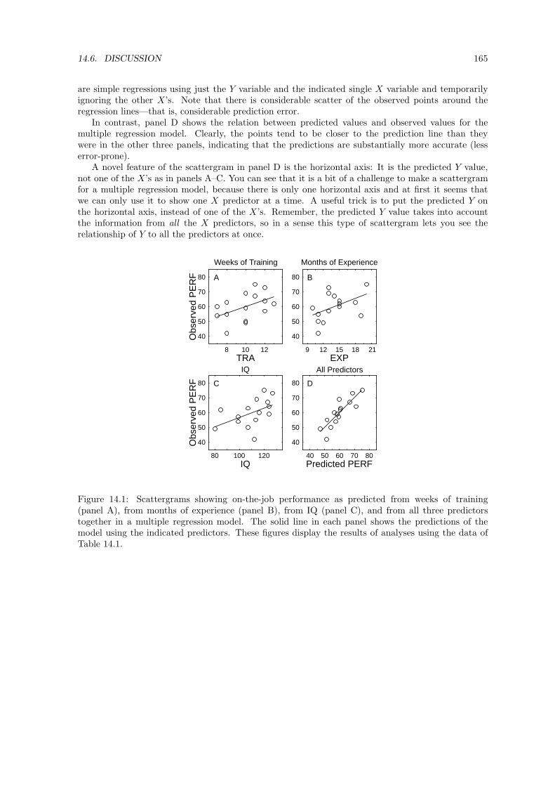
14.6. DISCUSSION 165
are simple regressions using just the Y variable and the indicated single X variable and temporarilyignoring the other X’s. Note that there is considerable scatter of the observed points around theregression lines—that is, considerable prediction error.
In contrast, panel D shows the relation between predicted values and observed values for themultiple regression model. Clearly, the points tend to be closer to the prediction line than theywere in the other three panels, indicating that the predictions are substantially more accurate (lesserror-prone).
A novel feature of the scattergram in panel D is the horizontal axis: It is the predicted Y value,not one of the X’s as in panels A–C. You can see that it is a bit of a challenge to make a scattergramfor a multiple regression model, because there is only one horizontal axis and at first it seems thatwe can only use it to show one X predictor at a time. A useful trick is to put the predicted Y onthe horizontal axis, instead of one of the X’s. Remember, the predicted Y value takes into accountthe information from all the X predictors, so in a sense this type of scattergram lets you see therelationship of Y to all the predictors at once.
8 10 12TRA
40
50
60
70
80
Obs
erve
dP
ER
F
Weeks of Training
A
9 12 15 18 21EXP
40
50
60
70
80
Months of Experience
B
80 100 120IQ
40
50
60
70
80
Obs
erve
dP
ER
F
IQ
C
40 50 60 70 80Predicted PERF
40
50
60
70
80
All Predictors
D
Figure 14.1: Scattergrams showing on-the-job performance as predicted from weeks of training(panel A), from months of experience (panel B), from IQ (panel C), and from all three predictorstogether in a multiple regression model. The solid line in each panel shows the predictions of themodel using the indicated predictors. These figures display the results of analyses using the data ofTable 14.1.

166 CHAPTER 14. MULTIPLE REGRESSION

Chapter 15
Extra Sum of Squares Comparisons
15.1 Overview and Example
As already discussed, a limitation of multiple regression models is that they only provide an overallF to test whether the Y variable is predicted by the model as a whole, including all its predictorvariables. Usually, it much more important to separate out the individual contributions of specificpredictor variables. The technique of making extra sum of squares comparisons (ESSCs, for short)provides a way to do this, at least to some extent.
You might wonder why we need a new technique to look at the contributions of individualpredictors, given that we have already seen how a simple one-variable regression can be used tostudy the relation between Y and an individual predictor. The reason goes back to the discussionof soccer versus cricket in Section 14.3. Different predictors work together to predict Y in multipleregression, just as different players work together to score in soccer. By looking at an individualpredictor in a one-variable regression, all we can tell is how well that predictor does on its own. Thenew technique will enable us to see how well a certain predictor does as part of a certain team, andthat is different. This idea will be illustrated with a further example soon.
Computationally, an ESSC is always a comparison between two regression models. There is a“smaller model” with a certain set of predictors, and it is compared against a “larger model” withthat same set of predictors plus at least one extra predictor. The test allows you to determine whetherthe larger model is significantly better than the smaller model; if so, you can conclude that the extrapredictor(s) do indeed make significant separate and unique contributions to the overall prediction.
For example, suppose you are trying to determine whether students’ success in a statistics classdepends on their knowledge of maths. One simple study would be:
Study 1: At the beginning of a statistics class, you give each student a maths achievement test(MAT). At the end of the statistics class, you obtain each student’s percentage mark for theclass (STAT). You then carry out a simple linear regression to try to predict STAT from MAT.
If it turns out that knowledge of maths does not predict statistics marks, you will conclude thatstatistics marks do no strongly depend on knowledge of maths, subject to the usual caveats.
If it turns out that knowledge of maths does predict statistics marks, however (as seems likely!),your conclusions will be weaker. This result is consistent with the idea that success in statistics doesdepend on maths knowledge, but it is very weak support for that idea because you have ignored anobvious mediating factor: namely, overall ability (as opposed to math-specific ability, which you claimto be focusing on). It could be that high-ability students tend to do better in all subjects, and thatthe relationship between maths knowledge and statistics marks results from the common influenceof ability on both of them, not from an influence of maths knowledge on statistics scores. To putit more concretely, we might have found just as strong a relationship to STAT if we had measuredachievement on a verbal test or a history test, instead of a maths test. Thus, we cannot be sure thatsuccess in statistics really depends on knowledge of maths per se.
A better study could be conducted to try to control for overall student ability as follows:
Study 2: At the beginning of a statistics class, you give each student a maths achievement test(MAT). You also obtain their overall average score in other university classes (AVG) as a measureof overall ability. At the end of the statistics class, you obtain each student’s percentage markfor the class (STAT). Now, you use multiple regression to see how the statistics mark is related
167

168 CHAPTER 15. EXTRA SUM OF SQUARES COMPARISONS
to both of the other two variables. Specifically, the question is whether STAT is specificallyrelated to knowledge of maths beyond what is explainable in terms of overall ability (AVG).This question can be answered with an ESSC, even though it cannot be answered by the simpleregression of Study 1.
A hypothetical data set for Study 2 is shown in Table 15.1. As discussed in Chapter 14, you canobtain the best-fitting two-predictor multiple regression model from a computer program, which forthese data yields the model:
STAT = −6.724 + 0.422 × MAT + 0.644× AVG (15.1)
Then, these a and b values can be used to compute the predicted values and errors shown in Table 15.1.The overall summary ANOVA for the two-predictor regression is shown in Table 15.2.
Case STAT MAT AVG Predicted Error1 67 70 75 71.12 = -6.72 + 0.42 × 70 + 0.64 × 75 -4.12 = 67 - 71.122 56 62 66 61.94 = -6.72 + 0.42 × 62 + 0.64 × 66 -5.94 = 56 - 61.943 62 61 67 62.17 = -6.72 + 0.42 × 61 + 0.64 × 67 -0.17 = 62 - 62.174 65 62 74 67.10 = -6.72 + 0.42 × 62 + 0.64 × 74 -2.10 = 65 - 67.105 85 79 80 78.13 = -6.72 + 0.42 × 79 + 0.64 × 80 6.87 = 85 - 78.136 80 74 88 81.18 = -6.72 + 0.42 × 74 + 0.64 × 88 -1.18 = 80 - 81.187 77 68 70 67.05 = -6.72 + 0.42 × 68 + 0.64 × 70 9.95 = 77 - 67.058 75 66 76 70.07 = -6.72 + 0.42 × 66 + 0.64 × 76 4.93 = 75 - 70.079 59 53 58 52.99 = -6.72 + 0.42 × 53 + 0.64 × 58 6.01 = 59 - 52.99
10 64 65 79 71.58 = -6.72 + 0.42 × 65 + 0.64 × 79 -7.58 = 64 - 71.5811 67 57 71 63.05 = -6.72 + 0.42 × 57 + 0.64 × 71 3.95 = 67 - 63.0512 73 74 78 74.74 = -6.72 + 0.42 × 74 + 0.64 × 78 -1.74 = 73 - 74.7413 67 66 71 66.85 = -6.72 + 0.42 × 66 + 0.64 × 71 0.15 = 67 - 66.8514 62 71 75 71.54 = -6.72 + 0.42 × 71 + 0.64 × 75 -9.54 = 62 - 71.5415 55 61 67 62.17 = -6.72 + 0.42 × 61 + 0.64 × 67 -7.17 = 55 - 62.1716 78 57 88 74.00 = -6.72 + 0.42 × 57 + 0.64 × 88 4.00 = 78 - 74.0017 77 74 70 69.58 = -6.72 + 0.42 × 74 + 0.64 × 70 7.42 = 77 - 69.5818 58 68 62 61.90 = -6.72 + 0.42 × 68 + 0.64 × 62 -3.90 = 58 - 61.90
Sum: 1227.00 1227.00 0.00Mean: 68.17 68.17 0.00
SumSq: 85003.00 84433.85 569.15
Table 15.1: Hypothetical data for a sample of 18 students. The goal was to find out whether thestudent’s mark in a statistics class (STAT) was related to their knowledge of maths (MAT), alsotaking into account their overall average university mark (AVG). A computer program reports thatthe best-fitting two-predictor model is STAT = −6.724+0.422×MAT+0.644×AVG, and the predictedvalues and error were computed using this model.
SSµ = 18 × 68.17 × 68.17 = 83640.50
SSmodel = 84433.85− 83640.50 = 793.35
SSerror = 569.15
SScorrected total = 85003.00− 83640.50 = 1362.50
Source df SS MS FModel 2 793.35 396.68 10.45Error 15 569.15 37.94Total 17 1362.50
Table 15.2: Further multiple regression computations and summary ANOVA table for the two-predictor model shown in Table 15.1.
For this example, the significant Fmodel in Table 15.2 indicates that the two-predictor model doesindeed predict statistics marks at a better-than-chance level. Of course this is not at all surprising.Even if statistics mark were totally unrelated to maths knowledge, we would still expect STAT tobe predictable from AVG. Students with higher overall marks averaged across all classes should scorerelatively well in statistics classes too; the motivation, intelligence, study habits, and so on that helpedthem do well in other classes should also tend to help in statistics. Thus, the overall Fmodel tells usnothing about whether statistics marks depend specifically on maths knowledge.

15.2. COMPUTATIONS 169
Within the context of this example, the crucial question is whether maths knowledge makes asignificant unique contribution to the predictions of the two-predictor model. What we really wantto know is whether we can predict better using both AVG and MAT than just using AVG by itself.If so, it must be because statistics mark is specifically related to maths knowledge, not just relatedto average overall mark of all types. In short, the question is whether we really need MAT in thetwo-predictor model.
This is exactly the sort of question that the ESSC was designed to answer. In terms of ourearlier definition, the smaller model is the model with just AVG, and the larger model uses bothAVG and MAT. By comparing these two models, we can see if MAT improves predictions beyondthose available from just AVG. If it does, then we can conclude that the data demonstrate a separatepredictive contribution of MAT, above and beyond the predictive ability provided by AVG.
15.2 Computations
Table 15.3 provides a schematic diagram of the extra sum of squares comparison. The middletwo columns of the table represent the smaller and the larger of the two models being compared,respectively. Listed in each column are the model’s predictors, its sum of squares, and its dfs. Thecolumn at the far right represents the comparison between the two models, listing on each line theadditional or “extra” portion that is present in the larger model but not in the smaller one. The mostcrucial value in this column is the “extra sum of squares” or SSextra. Intuitively, this represents theimprovement in predictability brought about by adding the extra predictor(s) into the model, overand above the predictability obtainable with the smaller model. The F in the lower panel of the tablewill be explained in a moment.
Table 15.5 shows how these columns are filled in for the extra sum of squares comparison to seewhether MAT improves the prediction of STAT over and above using only AVG.
• The smaller model is the one-predictor model predicting STAT from AVG. Its sum of squaresand degrees of freedom are computed using the standard formulas associated with a simple (i.e.,one-predictor) regression, computed as if STAT and AVG were the only two variables in thedata set. This model and its ANOVA table are shown in Table 15.41. The SS and df for thismodel are simply copied from that table into the “smaller model” column of Table 15.5.
• The larger model is the two-predictor model summarized in Table 15.2. Its sum of squares anddegrees of freedom are copied into the “larger model” column of Table 15.5.
• The right-most column is then formed by taking the difference between the second and thirdcolumns. Intuitively, the “extra sum of squares” in this column represents the improvement inpredictability due to adding MAT, over and above the predictability obtainable from just AVG.
Extra Sum of Squares Comparison:Smaller model Larger model Extra
Predictors: smaller set smaller set additional additionalSS model: SSsmaller SSlarger SSextra = SSlarger − SSsmaller
df model: dfsmaller dflarger dfextra = dflarger − dfsmaller
Extra F =SSextra/dfextra
MSerror, larger model= Fobserved for additional predictors
Table 15.3: The general pattern used in making an extra sum of squares comparison.
As in this example, the SSlarger is always numerically larger than the SSsmaller , so the SSextra isalways positive. Conceptually speaking, the larger model always does at least a little bit better. Butthis may be just due to chance, because it has an extra degree of freedom to use in fitting the data.The question is: Is the larger model enough better that we can exclude chance as the explanation ofthe improvement?
To answer this question, we compute an Extra F . The general version of the Extra F computationis shown at the bottom of Table 15.3. The numerator of the Extra F is the SSextra divided by the
1We will not describe the computation of this simple regression because this topic has already been covered.

170 CHAPTER 15. EXTRA SUM OF SQUARES COMPARISONS
STAT = 10.40 + 0.79 × AVG
Source df SS MS FModel 1 669.62 669.62 15.46Error 16 692.88 43.30Total 17 1362.50
Table 15.4: Summary ANOVA table for a simple regression model predicting STAT from AVG withthe data shown in Table 15.1.
Extra Sum of Squares Comparison:Smaller model Larger model Extra
Predictors: AVG AVG MAT MATSS model: 669.62 793.35 123.73df model: 1 2 1
Extra F =123.73/1
37.94= 3.26 for adding MAT
Table 15.5: Computation of extra sum of squares comparison to see whether success in statistics isrelated to knowledge of maths.
dfextra, often called the “extra mean square” or MSextra2. The denominator is always the MSerror
from the larger model. It makes sense to use the MSerror from the larger model rather than from thesmaller model, because the smaller model’s MSerror could be inflated (thereby reducing the F andthe chances of a significant result) if it ignores important predictors that are included in the largermodel. (This comment about inflating error will be clearer after we have covered the topic of “errorreduction” in section 16.3, but for now just make the analogy to ANOVA: If we omitted factors froman ANOVA, their effects went into the error term and reduced F ’s and power.)
An example of the Extra F computation is shown at the bottom of Table 15.5. The SSextra
and dfextra in the numerator of the F are taken directly from the right-most column of the table.The MSerror in the denominator is taken from the ANOVA table summarizing the fit of the largermodel—in this case, Table 15.2.
As usual, the Extra F is compared against a critical F from the F table. The critical F hasdfextra degrees of freedom in the numerator, because the MSextra is associated with dfextra degreesof freedom. In the denominator, it has the number of degrees of freedom associated with the MSerror
of the larger model, which is the number of cases minus one minus the number of predictors in thelarger model. In the current example, then, the critical F has 1 and 15 dfs, so Fcritical = 4.54. Theobserved F of 3.26 is less than Fcritical, so the null hypothesis is not rejected.
15.3 Conclusions & Interpretation
15.3.1 The Null Hypothesis
The Extra F tests the null hypothesis that:
the extra predictors add nothing to the predictability of Y given that the predictors inthe smaller model are already being used.
In terms of the parameters of the model, this can also be stated as:
the true values of the b’s for the added predictors in the larger model are really zero.
In terms of a model comparison, this can also be stated as:
the larger model is really no better than the smaller model.
2In most situations the larger model has just one more predictor than the smaller one, so the dfextra is one and theMSextra equals the SSextra. But if the larger model has two or more extra predictors relative to the smaller one, theextra sum of squares has to be divided by the number of extra predictors, just as all sums of squares are divided bytheir degrees of freedoms before computation of an F . See Section 15.4.3 for an example.

15.3. CONCLUSIONS & INTERPRETATION 171
15.3.2 Interpretation of a Significant Extra F
When the Extra F is significant, the interpretation is:
There is a separate predictive relationship between Y and at least one of the extrapredictors beyond that explainable in terms of the predictors in the smaller model. This isconsistent with the hypothesis that one or more of the extra predictors has an additionalcausal influence on Y beyond any influences related to the X’s in the smaller model. Thecausal influence is not proved, however, because there may be other mediating variablesnot included in the smaller model.
As a matter of terminology, common alternative phrasings of this conclusion sound like this:
• There is a separate predictive relationship between Y and the extra predictors that is not mediatedby the predictors in the smaller model.
• There is a separate predictive relationship between Y and the extra predictors controlling forthe predictors in the smaller model.
• There is a separate predictive relationship between Y and the extra predictors taking into accountthe predictors in the smaller model.
• There is a separate predictive relationship between Y and the extra predictors partialling outthe predictors in the smaller model.
All of these phrasings refer to the same extra sum of squares comparison.In the example involving the statistics mark, if the extra F had been significant the interpretation
would have been:
There is a significant predictive relationship between maths knowledge and statisticsmark “beyond that explainable in terms of” overall average university mark (or “notmediated by” or “controlling for”). That is, we know that the relationship betweenstatistics marks and maths knowledge is not completely explainable as “better overallstudents have more maths knowledge and also get better statistics marks.” (This rules outthe mediating variable explanation that would have contaminated Study 1, as discussedearlier.) The unique relationship of maths knowledge and statistics mark, controlling foroverall average, is consistent with the idea that statistics mark is causally determined bymaths knowledge. That causal relationship is not proved, however, because perhaps someother variable mediates the relationship between statistics marks and maths knowledge.
What other variable might mediate this relationship? Here is one possible scenario: Suppose thatwhat really makes people good at statistics is a tendency to think in a very orderly fashion, and this“mental orderliness” also tends to make them score higher on the maths test. In that case MATand STAT could be related because both were causally determined by orderliness, not because mathknowledge had a causal influence on statistics mark. So, orderliness could be the mediating variablein this case. In the end, if you really want to be certain of a causal relationship, then you just haveto do an experiment:
Experiment: Assign students randomly to two groups. Pre-teach the students in one group (“highmaths knowledge group”) some extra maths, and teach the other group (“control group”)something else (Latin?) to control for placebo effects, generalized learning experience, andso on. After both groups had been pre-taught, teach them statistics and see if their statisticsperformance levels were different at the end.
Obviously, this experiment is much more work than either of the correlational studies described earlier,because of the pre-teaching that is required.
But before we go on, here is some reassurance for the mathematically challenged: Take heart, thisF is generally not significant in real studies looking at this relationship (e.g., Ware & Chastain, 1989).That is, real data do not suggest any specific relationship between maths skill and statistics mark.

172 CHAPTER 15. EXTRA SUM OF SQUARES COMPARISONS
15.3.3 Interpretation of a Nonsignificant Extra F
When the Extra F is not significant, the interpretation is:
There is no clear evidence of a separate predictive relationship between Y and the extrapredictors beyond that explainable in terms of the predictors in the smaller model. This isconsistent with the hypothesis that none of the extra predictors has an additional causalinfluence on Y beyond the influences related to the X’s in the smaller model. The absenceof a causal influence is not proved, however, because the causal relationship may have beentoo weak to detect with the actual sample size or may have been concealed by poolingeffects, large measurement error, range restriction, etc.
In the example involving the statistics mark, the interpretation of the nonsignificant is:
There is no clear evidence of a significant predictive relationship between maths knowledgeand statistics mark beyond that explainable in terms of overall average university mark.This is consistent with the idea that statistics mark is not causally determined by mathsknowledge. The absence of a causal relationship is not proved, however, because the causalrelationship may have been too weak to detect with the actual sample size or may havebeen concealed by pooling effects, large measurement error, range restriction, etc.
15.4 Discussion
15.4.1 Measurement by subtraction.
The idea of an extra sum of squares comparison is a new version of an old, familiar procedure:Measurement by subtraction. For example, how would you determine the weight of a liter of oil?You would find a large enough container, weigh it empty, pour in the oil, weigh it again, and see howmuch the weight had gone up. That’s quite analogous to an extra sum of squares comparison, exceptyou are measuring weight rather than “sum of squares explained by the model.” The container isanalogous to the smaller model: First, you measure it by itself. Then you add the portion you arereally interested in (oil or predictors), and measure the new total. Finally, the two measurements aresubtracted, and the difference is taken as the measurement of the added part.
Measurement by subtraction also underlies most before/after comparisons. Suppose you test yourstrength in January, undergo a weight-training program for six months, and then test your strengthagain in July. The difference in strength from before to after would be a measure of the effectivenessof the program. Your original self is the smaller part, and yourself augmented by the training programis the larger one, with an increment due to the program.
Another example, discussed in Chapter 14, was the example of measuring a player’s offensivecontribution in a game where players must work together to score, like soccer. Although impracticalat best, the idea of measurement by subtraction could be applied in this case as well. Imagine thatwe wanted to evaluate Joe Bloggs’s offensive contribution. We could have Joe’s team play (say) eightgames against another team, with Joe playing in four of the games and sitting out the other four. Wecould then find the difference between the points scored by his team when he was playing minus thepoints scored by those same players when he was sitting out. Obviously, if the team scored lots morewhen he was playing, then he must have been making a big contribution to the scoring—even if henever actually scored a goal personally3.
15.4.2 Controlling for potential confounding variables.
Extra sum of squares comparisons allow you to examine the relationship between Y and a certain Xvariable (or group of X variables) controlling for the effects of certain other X variables. In essence,this allows you to take into account some of the confounding or mediating variables that weakeninterpretations in correlation and regression analysis. When they are taken into account, they areeliminated as alternative explanations.
In the statistics mark study, for example, you could see whether there was a specific relationbetween statistics mark and math knowledge that was not just due to the correlation of both of thesevariables with overall university mark, which presumably takes account of various general study habits,
3I am assuming that eight games would be enough for the averages to be pretty stable (i.e., for random error tomostly average out). If not, we’d need more games, but the basic idea would be the same.

15.4. DISCUSSION 173
etc, that are not specifically associated with math knowledge. If you got a significant STAT/MATrelationship after you eliminated this mediating correlation, you would have better evidence thatmaths knowledge really does causally influence statistics mark (better than if you had not eliminatedthis mediating variable).
As another example, suppose you were investigating the relationship between life expectancy andcoffee drinking. For each person in your sample, you record how long they lived and also somehowdetermine how much coffee they drank. Computing a simple regression, you find that life expectancyis significantly negatively associated with amount of coffee drunk. In other words, people who drinkmore coffee do not live as long. Of course you cannot conclude that there is a causal relationship—thatdrinking lots of coffee shortens your life. This is because the coffee/life-expectancy relationship couldbe mediated by some other variable—very possibly amount smoked. We know that people who tendto smoke more also tend to drink more coffee, and it could be the extra smoking rather than the extracoffee that is reducing life expectancy. This is one possible way to explain the coffee/life-expectancyrelationship without a direct causal link from coffee to health.
To rule out this explanation of the coffee/life-expectancy relationship, you could measure smokingand control for it statistically. In practice, this means making an extra sum of squares comparisonof the form shown in Table 15.6. The smaller model includes just the amount smoked, which isthe variable you want to control for. The larger model includes amount of coffee drunk in addition.Thus, the difference is a measure of the specific predictive association between coffee drinking and lifeexpectancy beyond that mediated by the amount smoked.
Extra Sum of Squares Comparison:Smaller model Larger model Extra
Predictors: SMOK SMOK COFF COFFSS model: SSSMOK SSSMOK+COFF SSextra = SSCOFF
df model: 1 2 1
Extra F =SSextra/1
MSerror, larger model= Fobserved for COFF
Table 15.6: Format of a possible extra sum of squares comparison to test for a specific effect of amountof coffee drunk (COFF) on life expectancy, controlling for amount smoked (SMOK).
15.4.3 When would you use more than one “extra” predictor?
In all of the comparisons discussed so far, the larger model has exactly one more predictor than thesmaller model, and indeed this is by far the most common situation. However, the basic idea of theESSC can also be applied to evaluate the specific contribution of a group of variables, simply bycomparing a smaller model against a larger model with more than one additional variable. This isusually done only when a group of variables all measure the same sort of thing.
For example, suppose we were trying to evaluate environmental and genetic contributions to IQ.We obtain a sample of adopted children, measure their IQs, the IQs of their adoptive parents, and theIQs of their biological parents. In principle we could measure both mothers’ and fathers’ IQs, yieldinga data set containing five variables:
• Child’s IQ (Y)
• AdoM, Adoptive mother’s IQ (X1)
• AdoF, Adoptive father’s IQ (X2)
• BioM, Biological mother’s IQ (X3)
• BioF, Biological father’s IQ (X4)
With respect to our interest in environmental versus genetic determinants of IQ, it seems clear thatwe have two predictors of each type: The adoptive mother’s and father’s IQs should be related to thechild’s IQ to the extent that there is an environmental influence. Conversely, the biological mother’sand father’s IQs should be related to the extent that there is a genetic influence. Because the variablesare paired up like this, it would be sensible to make extra sum of squares comparisons evaluating the

174 CHAPTER 15. EXTRA SUM OF SQUARES COMPARISONS
specific predictive contributions of both environmental predictors at once, as shown in Table 15.7, orof both genetic predictors at once, as shown in Table 15.8.
Extra Sum of Squares Comparison:Smaller model Larger model Extra
Predictors: BioM+BioF BioM+BioF AdoM+AdoF AdoM+AdoFSS model: SSBioM+BioF SSBioM+BioF+AdoM+AdoF SSextra = SSAdoM+AdoF
df model: 2 4 2
Extra F =SSextra/2
MSerror, larger model= Fobserved for AdoM+AdoF
Table 15.7: Format of a possible extra sum of squares comparison to test for evidence of a specificenvironmental effect on IQs of adopted children.
For example, Table 15.7 shows the ESSC to test for an environmental influence on IQ. Both of the“genetic” predictors are in the smaller model, so they are controlled for in the comparisons. Then,both of the environmental variables are added at once, so we can see if knowing a lot about theenvironment improves the prediction.
Suppose this ESSC yields a significant extra F . In that case, we could conclude that there is aunique relationship between the child’s IQ and the IQ of at least one of the adoptive parents, aboveand beyond any relationship of the child’s IQ with the IQs of its biological parents. This wouldsupport the idea that IQ is at least partly determined by the environment.
On the other hand, suppose this ESSC does not yield a significant extra F . In that case, we couldconclude that neither of adoptive parents’ IQs has a separate, unique relationship to the child’s IQ,above and beyond any relationship of the child’s IQ with the IQs of its biological parents. This wouldbe consistent with the idea that IQ is not very strongly determined by the environment.
Extra Sum of Squares Comparison:Smaller model Larger model Extra
Predictors: AdoM+AdoF AdoM+AdoF BioM+BioF BioM+BioFSS model: SSAdoM+AdoF SSAdoM+AdoF+BioM+BioF SSextra = SSBioM+BioF
df model: 2 4 2
Extra F =SSextra/2
MSerror, larger model= Fobserved for BioM+BioF
Table 15.8: Format of a possible extra sum of squares comparison to test for evidence of a specificgenetic effect on IQs of adopted children.
Conversely, suppose the extra sum of squares comparison in Table 15.8 yields a significant F .In that case, we could conclude that the IQs of the biological parents do have a separate, uniquerelationship to the child’s IQ, above and beyond any relationship of the child’s IQ with the IQs of itsadoptive parents. This would support the idea that IQ is at least partly determined by genetics. Ofcourse it is possible that IQ is determined by both the environment and genetics, in which case bothof the preceding extra sum of squares comparisons might be significant.
In summary, it makes sense to add two or more predictor variables together when you think theyall reflect the type of effects you are trying to assess—e.g., environmental or genetic.
15.5 Fadd and Fdrop
The extra sum of squares comparison plays such an important role in regression analysis that itsF value is referred to with different names in different situations (just as the Eskimos have severaldifferent words for snow). This section explains the most common alternative names for the “extraF”. The alternatives will be used extensively in Chapter 17.
As we have seen, the extra sum of squares comparison always involves a larger model and a smallermodel. The comparison can be stated as either:
• “Is the larger model better than the smaller one?” or

15.5. Fadd AND Fdrop 175
• “Is the smaller model worse than the larger one?”
Even though these two statements are equivalent mathematically, in practice many people usedifferent terminology depending on whether the smaller model was fit first, and then the larger, or thereverse. As summarized in Table 15.9, when the smaller model is fit first and the larger is fit second,the Fextra is often called an “F to add” or an “F to enter.” When the larger model is fit first and thesmaller is fit second, the Fextra is called an “F to drop” or an “F to remove.”
Order of model fits Names for Fextra
Smaller then larger “F to add” or “F to enter”Larger then smaller “F to drop” or “F to remove”
Table 15.9: Terminology for the Fextra depending on the order of model fits.
Sometimes, the distinction between adding and dropping variables is inherent in the type of analysisbeing carried out. You will see some examples of this in Chapter 17, which presents some proceduresfor building good regression models by adding or dropping one predictor at a time.
At other times, the distinction between adding and dropping variables is really only a matter ofperspective, like the cup that is half empty or half full. As an example of how perspective plays arole, the following two cases illustrate two slightly different situations where you would be more likelyto talk about the “F to add” (case 1) or the “F to drop” (case 2). Clearly, the situations are notvery different, and you would be getting the same F value from the same ESS comparison in bothcases. Because of your slightly different perspective in the two cases, however, you would probablyuse different terms to describe this F .
Case 1: A researcher named Joe Bloggs proposes that IQ is determined only by genetics, not by theenvironment. You are skeptical and want to show that the environment also plays a role. So,you first fit a model predicting IQ from genetic variables alone, and then show that adding inenvironmental variables makes the model predict significantly better.
In this example, the “starting model” is the smaller, genetics-only model proposed by JoeBloggs. Your focus is on showing that the model is improved by the addition of the extraenvironmental variables. Thus, to emphasize your point, you might well describe the significantFextra as a significant “F -to-add” for the environmental variables. The phrase “F -to-enter” isused equivalently; the idea is that the model is improved by entering additional predictors intoit.
Case 2: A researcher named Joe Bloggs proposes that IQ is determined by both genetics and theenvironment. You are skeptical and want to show that the environment plays no role. So, youfirst fit a model predicting IQ from both types of variables, and then show that removing theenvironmental variables does not make the model predict significantly worse.
In this example, the “starting model” is the larger model with both types of predictors, asproposed by Joe Bloggs. Your focus is on showing that the model is not worsened by removingthe environmental variables. Thus, to emphasize your point, you might well describe thenonsignificant Fextra as a nonsignificant “F -to-drop” for the environmental variables. The phrase“F -to-remove” is used equivalently; the idea is that the model not worsened by removing certainpredictors from it.

176 CHAPTER 15. EXTRA SUM OF SQUARES COMPARISONS

Chapter 16
Relationships Among Predictors
Thus far, we have concentrated on the relationship between Y and each of the predictors used in themultiple regression model. In this chapter, we consider something of equal importance in multipleregression analysis: the relationships of the different predictor variables to one another. To simplify thediscussion, we will for the time being consider only situations where Y has positive or zero correlationswith all the predictors variables. After analyzing the effects of various types of relationships in thissimpler situation first, we will consider in Section 16.6 what happens when Y is negatively correlatedwith some of the predictors.
16.1 Context Effects
This chapter discusses several specific patterns of results that can arise when extra sum of squarescomparisons are made in multiple regression analysis. These are not the only possible patterns ofresults, but they are worthy of discussion because they can be quite puzzling. Some of the patternsare reasonably common, but at least one is quite rare. Nonetheless, they are all worth understanding,because they illustrate the different ways in which the relationships among predictors can influencethe results.
Each of the patterns is an illustration of what I call a “context effect.” A context effect occurswhen the apparent usefulness of a certain predictor depends on which other predictor variables areincluded in the model. In terms of an ESS comparison, I think of the predictors in the smaller modelas the “context” in which the extra predictor is being evaluated, and say that the context has an effectif F for that extra predictor changes depending on which variables are in the smaller model.
Context effects are puzzling because they violate our preconceptions about what sorts of results weare likely to get when we perform “measurement by subtraction.” Weighing a liter of oil, for example,you would expect to get just the same weight whichever container you used, because the weight ofthe container is supposed to cancel out in the subtraction. You would be very puzzled if you weighedthe same liter of oil in two different containers and found, for example, that it weighed twice as muchwhen measured in one container as when measured in another container. But exactly that sort ofeffect can happen in extra sum of squares comparisons—we will even see an example analogous tohaving the oil completely weightless in one measurement but quite heavy in another one!
As you can probably guess from the previous paragraph, weighing oil is not a great analogy foran extra sum of squares comparison in regression, even though it does illustrate measurement bysubtraction. The disanalogy is that oil has a “real” weight independent of its container. Predictorsdon’t, because the “unique” predictive relationship associated with a predictor depends on what otherpredictors are being used already. Evaluating Joe Bloggs’s contribution to a soccer team’s offense is abetter example, because you can imagine that his contribution would depend on which other playerswere used on his team. For example, he might fit very well with a team of highly aggressive andunpredictable players—he might contribute a lot to their scoring—and that team might score a lotmore with him than without him. Alternatively, he might fit very poorly with a team of more patientand methodical players, and they might score about as well without him as with him. The point isthat Joe’s “offensive contribution” is not just determined by his own characteristics, but also by howthese characteristics mesh with the other players on his team. The same is true for predictors, asillustrated by the various kinds of context effects discussed below.
177

178 CHAPTER 16. RELATIONSHIPS AMONG PREDICTORS
16.2 Redundancy
One puzzling pattern of results that can be obtained in a multiple regression situation is a combinationof these two basic outcomes:
1. A certain predictor, say X2, is a significant predictor of Y when considered as the only predictor.
2. The ESS for this predictor is not significant when the predictor is added to a smaller model withanother predictor, say X1.
Together, these two outcomes seem to create a paradox. The first outcome tells us that X2 is a goodpredictor of Y, and yet the second outcome tells us that X2 is not. How can these both be true?
In general terms, the explanation for this pattern is that X1 and X2 are redundant. By “redundant,”I mean that they convey approximately the same predictive information about Y. Since they conveythe same information, the model with both variables is not really any better than the model with justX1, producing the nonsignificant ESS comparison mentioned in outcome 2 above, even if X2 is a goodpredictor by itself.
As a silly example, suppose you wanted to predict people’s weights from two predictors: X1 isthe person’s height in centimeters, and X2 is his/her height in inches. Because taller people tend toweigh more, both X1 and X2 would be good predictors in isolation. Your predictions would be nobetter with both predictors than with just one, however, because the two predictors are completelyredundant—they both just measure height.
As a more realistic example, consider this thought problem that I’ve given to hundreds of studentsover the years. About three-quarters get it right—give it a try:
Imagine that you are trying to predict the heights of daughters. You have alreadymeasured one predictor variable—their mother’s heights. And now you are going tomeasure a second predictor variable which must be either (a) their maternal grandfather’sheight, or (b) their paternal grandfather’s height. Your problem is to choose whicheverone of these second predictors would help most with the predictions. Given that you arealready using the mother’s height, then, which second variable do you think would bebetter—the maternal or paternal grandfather?
My answer: It seems reasonable to assume that a daughter’s height is approximately equallydetermined by the genes from both sides of the family: her mother’s and her father’s. Once we usethe mother’s height as a predictor, we have excellent information about the genetic contribution fromthat side. Adding the maternal grandfather’s height would give us somewhat better information aboutthe mother’s side, but I suspect it would not help very much because we already know a lot about themother’s side (i.e., we know the mother’s side). In contrast, at this point we know nothing at all aboutthe father’s side. That’s why I’d prefer the paternal grandfather to the maternal one. In essence, I amsuggesting that a first person from the father’s side is likely to be more useful than a second personfrom the mother’s. That is, I think you would do better to use the paternal grandfather’s height asthe second predictor.
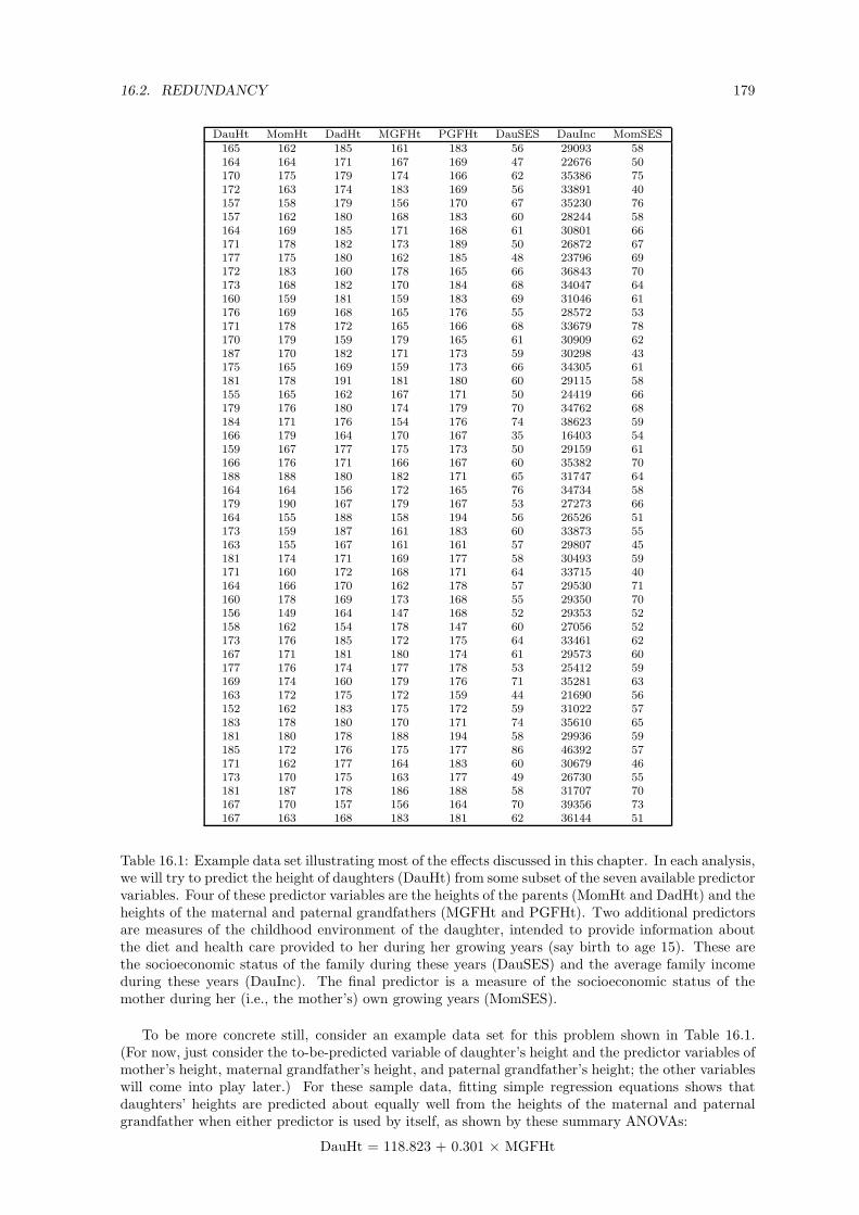
16.2. REDUNDANCY 179
DauHt MomHt DadHt MGFHt PGFHt DauSES DauInc MomSES165 162 185 161 183 56 29093 58164 164 171 167 169 47 22676 50170 175 179 174 166 62 35386 75172 163 174 183 169 56 33891 40157 158 179 156 170 67 35230 76157 162 180 168 183 60 28244 58164 169 185 171 168 61 30801 66171 178 182 173 189 50 26872 67177 175 180 162 185 48 23796 69172 183 160 178 165 66 36843 70173 168 182 170 184 68 34047 64160 159 181 159 183 69 31046 61176 169 168 165 176 55 28572 53171 178 172 165 166 68 33679 78170 179 159 179 165 61 30909 62187 170 182 171 173 59 30298 43175 165 169 159 173 66 34305 61181 178 191 181 180 60 29115 58155 165 162 167 171 50 24419 66179 176 180 174 179 70 34762 68184 171 176 154 176 74 38623 59166 179 164 170 167 35 16403 54159 167 177 175 173 50 29159 61166 176 171 166 167 60 35382 70188 188 180 182 171 65 31747 64164 164 156 172 165 76 34734 58179 190 167 179 167 53 27273 66164 155 188 158 194 56 26526 51173 159 187 161 183 60 33873 55163 155 167 161 161 57 29807 45181 174 171 169 177 58 30493 59171 160 172 168 171 64 33715 40164 166 170 162 178 57 29530 71160 178 169 173 168 55 29350 70156 149 164 147 168 52 29353 52158 162 154 178 147 60 27056 52173 176 185 172 175 64 33461 62167 171 181 180 174 61 29573 60177 176 174 177 178 53 25412 59169 174 160 179 176 71 35281 63163 172 175 172 159 44 21690 56152 162 183 175 172 59 31022 57183 178 180 170 171 74 35610 65181 180 178 188 194 58 29936 59185 172 176 175 177 86 46392 57171 162 177 164 183 60 30679 46173 170 175 163 177 49 26730 55181 187 178 186 188 58 31707 70167 170 157 156 164 70 39356 73167 163 168 183 181 62 36144 51
Table 16.1: Example data set illustrating most of the effects discussed in this chapter. In each analysis,we will try to predict the height of daughters (DauHt) from some subset of the seven available predictorvariables. Four of these predictor variables are the heights of the parents (MomHt and DadHt) and theheights of the maternal and paternal grandfathers (MGFHt and PGFHt). Two additional predictorsare measures of the childhood environment of the daughter, intended to provide information aboutthe diet and health care provided to her during her growing years (say birth to age 15). These arethe socioeconomic status of the family during these years (DauSES) and the average family incomeduring these years (DauInc). The final predictor is a measure of the socioeconomic status of themother during her (i.e., the mother’s) own growing years (MomSES).
To be more concrete still, consider an example data set for this problem shown in Table 16.1.(For now, just consider the to-be-predicted variable of daughter’s height and the predictor variables ofmother’s height, maternal grandfather’s height, and paternal grandfather’s height; the other variableswill come into play later.) For these sample data, fitting simple regression equations shows thatdaughters’ heights are predicted about equally well from the heights of the maternal and paternalgrandfather when either predictor is used by itself, as shown by these summary ANOVAs:
DauHt = 118.823 + 0.301 × MGFHt
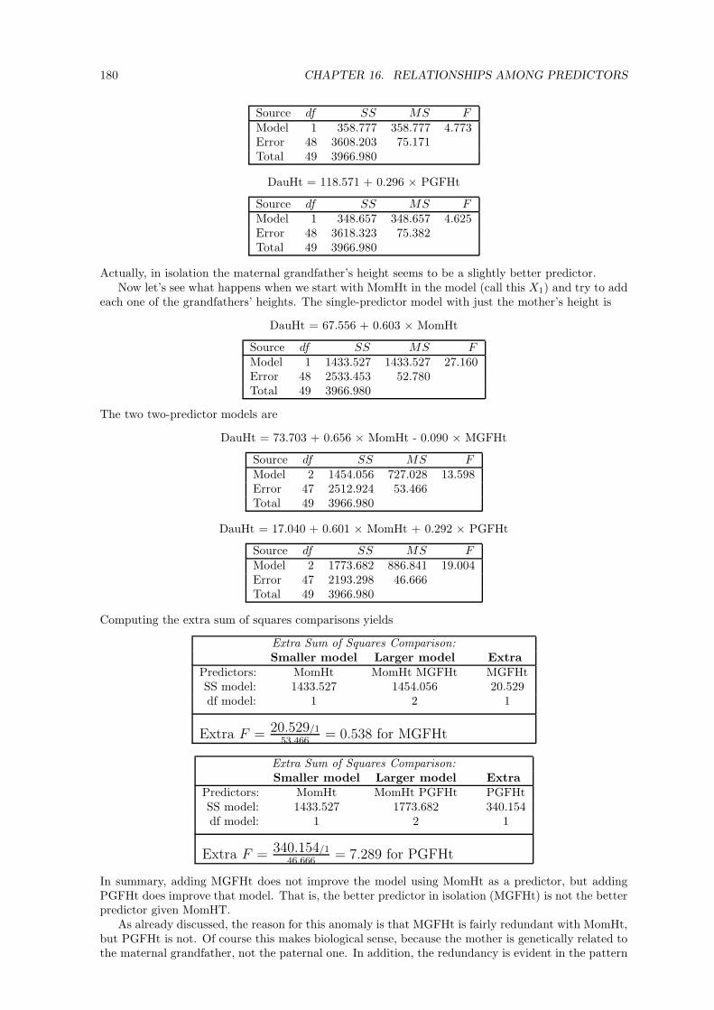
180 CHAPTER 16. RELATIONSHIPS AMONG PREDICTORS
Source df SS MS FModel 1 358.777 358.777 4.773Error 48 3608.203 75.171Total 49 3966.980
DauHt = 118.571 + 0.296 × PGFHt
Source df SS MS FModel 1 348.657 348.657 4.625Error 48 3618.323 75.382Total 49 3966.980
Actually, in isolation the maternal grandfather’s height seems to be a slightly better predictor.Now let’s see what happens when we start with MomHt in the model (call this X1) and try to add
each one of the grandfathers’ heights. The single-predictor model with just the mother’s height is
DauHt = 67.556 + 0.603 × MomHt
Source df SS MS FModel 1 1433.527 1433.527 27.160Error 48 2533.453 52.780Total 49 3966.980
The two two-predictor models are
DauHt = 73.703 + 0.656 × MomHt - 0.090 × MGFHt
Source df SS MS FModel 2 1454.056 727.028 13.598Error 47 2512.924 53.466Total 49 3966.980
DauHt = 17.040 + 0.601 × MomHt + 0.292 × PGFHt
Source df SS MS FModel 2 1773.682 886.841 19.004Error 47 2193.298 46.666Total 49 3966.980
Computing the extra sum of squares comparisons yields
Extra Sum of Squares Comparison:Smaller model Larger model Extra
Predictors: MomHt MomHt MGFHt MGFHtSS model: 1433.527 1454.056 20.529df model: 1 2 1
Extra F =20.529/1
53.466= 0.538 for MGFHt
Extra Sum of Squares Comparison:Smaller model Larger model Extra
Predictors: MomHt MomHt PGFHt PGFHtSS model: 1433.527 1773.682 340.154df model: 1 2 1
Extra F =340.154/1
46.666= 7.289 for PGFHt
In summary, adding MGFHt does not improve the model using MomHt as a predictor, but addingPGFHt does improve that model. That is, the better predictor in isolation (MGFHt) is not the betterpredictor given MomHT.
As already discussed, the reason for this anomaly is that MGFHt is fairly redundant with MomHt,but PGFHt is not. Of course this makes biological sense, because the mother is genetically related tothe maternal grandfather, not the paternal one. In addition, the redundancy is evident in the pattern

16.2. REDUNDANCY 181
of correlations among these variables, shown in Table 16.2. In the second row, we can see that theMGFHt and MomHt are strongly correlated (r = 0.60), which indicates that they measure the samething to a great extent. Really, there is little more to their redundancy than this high correlation.Conversely, PGFHt and MomHt are essentially uncorrelated (r = 0.01), which indicates that theymeasure quite different things. Based on the idea that we want to add predictors that bring in newinformation, then, it is obvious that we should prefer PGFHt over MGFHt when trying to improvethe model using MomHt. And of course it would work just the other way around if our initial modelhad included DadHt; in that case, it would be more helpful to add MGFHt to get new information,not PGFHt.
MomHt DadHt MGFHt PGFHt DauSES DauInc MomSESDauHt 0.601 0.247 0.301 0.296 0.293 0.293 -0.009MomHt -0.010 0.596 0.006 0.003 0.003 0.499DadHt -0.001 0.611 0.000 -0.012 -0.013MGFHt 0.004 0.005 0.006 -0.001PGFHt 0.004 -0.001 -0.013DauSES 0.898 0.209DauInc 0.204
Table 16.2: Correlation matrix for the data set shown in Table 16.1.
More generally, what this example is meant to illustrate is that you want to avoid redundancy whenyou are assembling multiple predictors. Even if a predictor is useful by itself, it is not necessarily usefulin combination with other predictors if it is redundant with those other predictors. As an extremeexample, suppose your first predictor of daughter’s height was the height of the mother in centimeters,and someone suggested that as a second predictor you should also use the height of the mother ininches. Common sense should tell you that this suggestion is silly. Adding this second predictor woulddo you no good, because once you have the mother’s height once, you don’t need it again. In otherwords, the second predictor is useless because it is redundant with another predictor already beingused.
16.2.1 SS Thinning
Redundancy can also be responsible for a second puzzling pattern of results that is sometimes obtained,represented by a combination of these two basic outcomes:
1. Each of two predictors, say X1 and X2, is a significant predictor of Y when considered as theonly predictor.
2. The multiple regression model containing both X1 and X2 is not significant.
Again we seem to have a paradox: From the single-predictor regressions, we can conclude that eachpredictor is useful in predicting Y at a better than chance level. The result of the two-predictorregression, however, is consistent with the view that neither predictor is useful. How can the two-predictor model fail to be significant if each predictor is significant in isolation?
An example of this arises when we try to predict daughters’ heights (DauHt) from the measuresof their environments during their growing years (DauSES and DauInc) using the data in Table 16.1.Here are the two single-predictor models and the two-predictor model:
DauHt = 152.430 + 0.293 × DauSES
Source df SS MS FModel 1 339.485 339.485 4.492Error 48 3627.495 75.573Total 49 3966.980
DauHt = 153.678 + 0.001 × DauInc
Source df SS MS FModel 1 340.505 340.505 4.507Error 48 3626.475 75.552Total 49 3966.980

182 CHAPTER 16. RELATIONSHIPS AMONG PREDICTORS
DauHt = 152.153 + 0.152 × DauSES + 0.0005 × DauInc
Source df SS MS FModel 2 358.225 179.112 2.333Error 47 3608.755 76.782Total 49 3966.980
Note that the two one-predictors models are both significant, but the two-predictor model is not.The explanation for this puzzling pattern has two parts. First, the two predictors are correlated
(i.e., redundant), so to some degree they provide the same information about Y. In the exampledata, for instance, there is a 0.9 correlation between DauSES and DauInc. Because of this strongcorrelation, the two-predictor model does only a little better than the one-predictor models (SSmodel’sof approximately 339 and 340 versus 358). Second, the dfmodel increases from one to two going fromthe one-predictor models to the two-predictor model. Since the SSmodel stays approximately the same,that means that the MSmodel drops approximately in half for the two-predictor model compared tothe one-predictor models (MSmodel’s of approximately 339 and 340 versus 179). This reduction inMSmodel is crucial, because the Fmodel is the ratio of the MSmodel to the MSerror. Although theMSerror is approximately the same for all three models, the F for the two-predictor model is onlyabout half of that for the one-predictor models, because of its extra dfmodel.
In summary, as you include more and more redundant predictors in a model, the SSmodel doesnot increase as fast as the dfmodel, so the Fmodel drops. You might say that the same SS is gettingthinned out by being spread over too many degrees of freedom. After there has been enough thinning(i.e., enough redundant predictors added), the Fmodel can eventually drop below the Fcritical, even ifeach of the predictors is significant individually.
Conceptually, thinning occurs because a regression model should be able to do better as morepredictors are added, even if only by chance. If added predictors are redundant, however, there isno improvement in prediction—not even by chance. As more and more redundant predictors areadded, eventually the model appears to be doing no better than you would expect by chance withthat number of predictors, and so it’s Fmodel may drop below the level needed for significance.
16.3 Reduction of Error in Y
A third puzzling pattern of results is essentially the opposite of the first one:
1. A certain predictor, say X2, is not a significant predictor of Y when considered as the onlypredictor.
2. The ESS for this predictor is significant when the predictor is added to a smaller model withanother predictor, say X1.
Now, the first outcome tells us that X2 is not a good predictor of Y, and yet the second outcome tellsus that X2 is. How can these both be true?
In the data of Table 16.1, the variables of DadHt and MomHt provide an example of this. Byitself, DadHt is not a significant predictor of DauHt, as indicated by this one-predictor model1:
DauHt = 126.771 + 0.249 × DadHt
Source df SS MS FModel 1 242.312 242.312 3.123Error 48 3724.668 77.597Total 49 3966.980
Yet DadHt does add significantly to MomHt as a predictor, as indicated by the following two-predictormodel and associated ESS comparison:
DauHt = 22.755 + 0.605 × MomHt + 0.255 × DadHt
Source df SS MS FModel 2 1688.315 844.158 17.412Error 47 2278.665 48.482Total 49 3966.980
1I agree this is not a very realistic example data set, because there is no obvious reason why the heights of daughtersshould be more strongly correlated with the heights of their mothers than with the heights of their fathers. The datawere constructed mainly to illustrate the various outcomes discussed in this chapter, not to be realistic.

16.4. SUPPRESSION OF ERROR IN X 183
Extra Sum of Squares Comparison:Smaller model Larger model Extra
Predictors: MomHt MomHt DadHt DadHtSS model: 1433.527 1688.315 254.788df model: 1 2 1
Extra F =254.788/1
48.482= 5.255 for DadHt
If DadHt is not significant by itself, how can it add significantly to MomHt?This pattern arises because MomHt reduces the error term, thereby allowing us to see the statistical
significance of DadHt, even though it is only weakly related to DauHt. Note that the one-predictormodel with DadHt has a MSerror of 77, whereas the two-predictor model with both parents’ heightshas a much smaller MSerror of 48. In essence, including MomHt as a predictor removed much apparenterror from the analysis. As always, having a smaller error term produces larger F ’s, because the errorterm is the divisor of the F ratio.
Note that the error reduction we are discussing here is the same idea as the error reduction wediscussed in connection with ANOVA. When a factor is omitted from an ANOVA, its effects go intothe error term, thereby reducing the F ’s for the other factors. Similarly, if an important variable (e.g.,MomHt) is omitted from a regression analysis, effects that it could explain are included in the errorterm and reduce F ’s for the other predictors.
16.4 Suppression of Error in X
A fourth puzzling pattern of results is characterized by these outcomes:
1. A certain predictor, say X2, has a correlation with Y of zero, or very nearly so.
2. The ESS for this predictor is significant when the predictor is added to a smaller model withanother predictor, say X1.
At first this looks like just an extension of the previous puzzling result, “Reduction of Error in Y”:A predictor X2 looks no good by itself, but is good when added to another predictor. This case ismore extreme, however, because the poor predictor actually has a zero correlation with Y, not a smallcorrelation that turns out to be significant when error is reduced. How could a predictor that has azero correlation with Y ever be a useful predictor? After all, multiple regression simply uses linearrelationships between Y and the X’s to predict Y. If there is not even a hint of a linear relationbetween Y and a certain X, how can that X possibly be a useful predictor?
In the data of Table 16.1, the variables of MomHt and MomSES provide an example. As shown inTable 16.2, the correlation of DauHt with MomSES is essentially zero. And indeed it makes sense thatthe height of the daughter should be unrelated to the socioeconomic status that the mother enjoyedwhen she was growing up, especially if there is considerable social mobility from one generation tothe next. The lack of relation between DauHt and MomSES can also be seen in this simple regressionpredicting DauHt from MomSES:
DauHt = 170.567 - 0.009 × MomSES
Source df SS MS FModel 1 0.328 0.328 0.004Error 48 3966.652 82.639Total 49 3966.980
Despite the zero correlation between DauHt and MomSES, MomSES is quite a good predictor toadd to a model with MomHt in it. Here is the single-predictor model with just MomHt, repeatedfrom above:
DauHt = 67.556 + 0.603 × MomHt
Source df SS MS FModel 1 1433.527 1433.527 27.160Error 48 2533.453 52.780Total 49 3966.980

184 CHAPTER 16. RELATIONSHIPS AMONG PREDICTORS
And here is the two-predictor model with MomHt and MomSES, plus the ESS comparison to evaluatethe effect of adding MomSES:
DauHt = 57.253 + 0.809 × MomHt - 0.412 × MomSES
Source df SS MS FModel 2 1938.854 969.427 22.466Error 47 2028.126 43.152Total 49 3966.980
Extra Sum of Squares Comparison:Smaller model Larger model Extra
Predictors: MomHt MomHt MomSES MomSESSS model: 1433.527 1938.854 505.327df model: 1 2 1
Extra F =505.327/1
43.152= 11.711 for MomSES
The ESS comparison yields a highly significant F for MomSES, despite the absence of any correlationwith Y.
This pattern of results is often called a “suppressor effect”, and the variable that is useful despitebeing uncorrelated with Y is called a “suppressor variable.” For example, in this case MomSES is thesuppressor variable.
The pattern arises because the suppressor variable suppresses error in the other predictor variable,thereby making the other variable even better correlated with Y. In the example of Table 16.1, theexplanation would go something like this:
MomHt is basically determined by two components: genetics plus the mother’s environmentduring her growth years. Now the genetic component will be passed along to the daughter,so this component is quite relevant for predicting the daughter’s height. For example, if themother is short because she has the genes to be short, then the daughter is quite likely to beshort as well. But the environment of the mother during her growing years is not directlyrelevant to the daughter’s height, so this is less relevant to predicting the daughter’s height.For example, if the mother is short because of malnutrition or disease during her growthyears, the daughter is not particularly likely to be short as well (assuming that the growingenvironments of successive generations are not too strongly correlated).
The implication of our “two-component” theory of height is that we could predict thedaughter’s height better if we could measure the mother’s “genetic height” instead of heractual height. That is, we would like to measure the height to which she should have grown,barring any unusual environmental circumstances. Unfortunately, we can’t measure that,because we don’t yet know how to relate genes to expected height. But we can attemptto arrive at the genetic component in a two-step process: first, we measure actual height;second, we remove the effects of environment by correcting for the mother’s SES. Basedon our two-component model, we should be left with just the genetic component of themother’s height, and this should be a better predictor of the daughter’s height than wasthe original MomHt.
To see how the regression model uses the mother’s SES to correct for environmental effects, it isinstructive to look closely at the two-predictor model:
DauHt = 57.253 + 0.809 × MomHt - 0.412 × MomSES
Note the b1 of 0.809 associated with MomHt. This tells us to predict that the daughter will be tallerwhen the mother is taller, which makes sense. Note also the b2 of -0.412 associated with MomSES,which tells us to predict that the daughter will be shorter when the mother had a higher SES. This iswhere the correction happens. When the mother has a high SES, 0.809 × MomHt is too much to addin to the predicted daughter’s height. In this case some of the mother’s tallness was probably due toenvironment rather than genetics, and the environmental component will not be passed along to thedaughter. So, when the mother’s SES was high, we need to take back some of the predicted tallnessassigned to the daughter. Note that we are not assuming any direct causal relationship between themother’s SES and the daughter’s height.

16.5. VENN DIAGRAMS—OPTIONAL SECTION 185
16.5 Venn Diagrams—Optional Section
This section uses Venn diagrams as a form of pictorial representation to help portray the relationshipsamong variables that lead to redundancy, error reduction, and suppressor effects. The materialpresented here is not used elsewhere in the book, but it may aid some readers in conceptualizingcontext effects.
X2
Y X1
Figure 16.1: Use of Venn diagrams to represent correlations between variables. Y and X1 are correlatedwith each other, but neither is correlated with X2.
In a Venn diagram, each variable is represented as a circle. Points inside the circle representfactors influencing the variable, and points outside the circle represent factors that do not influenceit. The extent of correlation between two variables is represented by the overlap between their circles,with higher correlation represented by greater overlap. This makes sense: If two variables have mostlycommon influences then it makes sense that they should be well correlated. In Figure 16.1, for example,X1 and Y are correlated, but X2 and Y are not. With respect to the prediction of Y from a given Xvariable, the part explained by the model is the part that overlaps with that X; the remainder of Y,not overlapping with that X, is unexplained error.
Y
X1
X2
Figure 16.2: A pictorial representation of redundancy.
Figure 16.2 shows a pictorial representation of redundancy using Venn diagrams. In Figure 16.2,redundancy is apparent in the fact that both of the predictors, X1 and X2, overlap with Y in prettymuch the same area. That is, both predictors have the same things in common with Y, so either oneof them—but not both—is needed to explain that aspect of Y.
Figure 16.3 depicts the error reduction situation with a Venn diagram. The key point is that X1
and X2 overlap with different components of Y. In the two-predictor model, the error in Y is the partthat is not overlapped by either X variable. Note that there is much less unexplained Y (i.e., error)when both variables are included in the model than when only one is, because the two predictors biteoff different pieces of Y. Thus, each X can reduce error for the other. Note also that X1 and X2 donot overlap with each other, so they are not redundant. This is the situation that maximizes errorreduction, although some error reduction could still occur if X1 and X2 overlapped slightly, as longas the area of overlap was small relative to the separate overlaps with Y.
Figure 16.4 shows a pictorial representation of suppression in terms of Venn diagrams. Y iscorrelated with X2 but not with the suppressor variable X1 (in the example, DauHt is Y, MomHt is

186 CHAPTER 16. RELATIONSHIPS AMONG PREDICTORS
YX1 X2
Figure 16.3: A pictorial representation of error reduction.
X2Y X1
Figure 16.4: A pictorial representation of error suppression. X1 improves the predictions of Y fromX2, because X1 eliminates some irrelevant information from X2, essentially allowing X2’s relevantpart to stand out better.
X2, and MomSES is X1). X1 is correlated with the part of X2 which it does not share with Y. Byincluding X1 in the model, we can essentially factor out some of the irrelevant part of X2 and moreaccurately predict Y from the remaining, relevant part of X2.
16.6 Mixing Positive and Negative Correlations
This section will discuss various possibilities where Y has a positive correlation with some predictorsbut a negative correlation with others. All of the same phenomena can still arise: redundancy, errorreduction, and error suppression. It is slightly more difficult to spot these phenomena, however,because the mixed signs of the correlations can be confusing.
16.6.1 Redundancy
Redundancy arises when two predictors are both related to the to-be-predicted variable in pretty muchthe same way. Interestingly, this can happen even when the two predictors are negatively correlated.
For example, consider trying to predict an athlete’s long jump distance from his or her performancein a 10K running race. Race performance could be measured as the total time needed to run the 10K(X1). Alternatively, it could be measured as the runner’s average speed for the race (X2; e.g., inkilometers per hour). Time and speed have an almost perfect negative correlation, because largerspeeds produce smaller times, and vice versa2. Despite the negative correlation, of course, we knowthat both X1 and X2 really measure the same thing: how fast the runner went.
Time SpeedJump distance -0.50 0.50Time -0.95
Table 16.3: Hypothetical correlation matrix for time and speed in a 10K race and long-jump distance.
Table 16.3 shows a plausible correlation matrix for Y, X1, and X2 in this example. There is a strongnegative correlation between time and speed, as already discussed. In addition, the correlations ofjump distance with the two predictors have different signs—one positive and one negative. We expect
2The correlation is not quite perfect because time and speed are not linearly related. For example, three runnersfinishing the race in 1, 2, or 3 hours would have average speeds of 10, 5, and 3.33 K per hour. Plotting these points ona scattergram reveals a nonlinear relationship.
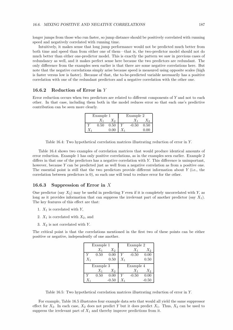
16.6. MIXING POSITIVE AND NEGATIVE CORRELATIONS 187
longer jumps from those who run faster, so jump distance should be positively correlated with runningspeed and negatively correlated with running time.
Intuitively, it makes sense that long jump performance would not be predicted much better fromboth time and speed than from either one of them—that is, the two-predictor model should not domuch better than either one-predictor model. This is exactly the pattern we saw in previous cases ofredundancy as well, and it makes perfect sense here because the two predictors are redundant. Theonly difference from the examples seen earlier is that there are some negative correlations here. Butnote that the negative correlations simply arise because speed is measured using opposite scales (highis faster versus low is faster). Because of that, the to-be-predicted variable necessarily has a positivecorrelation with one of the redundant predictors and a negative correlation with the other one.
16.6.2 Reduction of Error in Y
Error reduction occurs when two predictors are related to different components of Y and not to eachother. In that case, including them both in the model reduces error so that each one’s predictivecontribution can be seen more clearly.
Example 1 Example 2X1 X2 X1 X2
Y 0.50 0.50 Y -0.50 0.50X1 0.00 X1 0.00
Table 16.4: Two hypothetical correlation matrices illustrating reduction of error in Y.
Table 16.4 shows two examples of correlation matrices that would produce identical amounts oferror reduction. Example 1 has only positive correlations, as in the examples seen earlier. Example 2differs in that one of the predictors has a negative correlation with Y. This difference is unimportant,however, because Y can be predicted just as well from a negative correlation as from a positive one.The essential point is still that the two predictors provide different information about Y (i.e., thecorrelation between predictors is 0), so each one will tend to reduce error for the other.
16.6.3 Suppression of Error in X
One predictor (say X2) may be useful in predicting Y even if it is completely uncorrelated with Y, aslong as it provides information that can suppress the irrelevant part of another predictor (say X1).The key features of this effect are that:
1. X1 is correlated with Y,
2. X1 is correlated with X2, and
3. X2 is not correlated with Y.
The critical point is that the correlations mentioned in the first two of these points can be eitherpositive or negative, independently of one another.
Example 1 Example 2X1 X2 X1 X2
Y 0.50 0.00 Y -0.50 0.00X1 0.50 X1 0.50
Example 3 Example 4X1 X2 X1 X2
Y 0.50 0.00 Y -0.50 0.00X1 -0.50 X1 -0.50
Table 16.5: Two hypothetical correlation matrices illustrating reduction of error in Y.
For example, Table 16.5 illustrates four example data sets that would all yield the same suppressoreffect for X2. In each case, X2 does not predict Y but it does predict X1. Thus, X2 can be used tosuppress the irrelevant part of X1 and thereby improve predictions from it.

188 CHAPTER 16. RELATIONSHIPS AMONG PREDICTORS
Chapter 17
Finding the Best Model
In some situations a researcher has a large pool of potential predictor variables and just wants tosee how these can best be used to predict the variable of interest. This situation often arises inexploratory research, and there may be no specific hypotheses to test, contrary to our emphasis in theprevious regression chapters. For example, an educational researcher might be interested in findingout what predicts difficulties in learning to read, so that kids likely to have problems can be given aspecial head-start program. The to-be-predicted variable would be some available measure of readingproblems, and the researcher might use as predictors a whole host of different variables that caneasily be assembled from school records and other sources. Alternatively, a medical researcher mightbe interested in finding out what predicts susceptibility to a certain disease for which preventivemeasures are available. Or, a personnel psychologist might be interested in what predicts on-the-jobsuccess so that the best candidates can be selected for a certain job. Finally, a gambler might beinterested in predicting which of two teams will win a sporting event. In all of these cases, the goal issimply to come up with the best possible predictive model.
Mainly, this chapter presents some computational procedures that can be used when the problemis simply to find the best model. In using these procedures, you compute many F ’s using ESScomparisons. You do not interpret these F ’s, however (although you could interpret them as discussedin section 15.3, if you wanted to). Instead, in these procedures the F ’s are simply used to decide whatto do next.
In addition to the computational procedures, there are two conceptual points to consider: First,just what are the criteria for the “best” model? This point is considered in the next section. Second,how much faith should we have in the predictions from the best model after we find it? This point isconsidered in the final section.
17.1 What is the Best Model?
The first issue is exactly how we should define “the best model.” One goal is obviously to minimizeprediction error, but a second goal is also to keep the model as simple as possible. If they were equallyaccurate, we would certainly prefer a two-predictor model to a twenty-predictor model, because itwould be easier to use (i.e., you would only have to measure 2 predictors, not 20). A third goal is tohave a model that works well not only on the current cases but also on future cases to which we maywant to apply it, as discussed in Section 13.4. There is some room for debate about exactly how tocombine these goals in defining what the best model is, but in practice people pretty much seem toaccept the following operational definition. The best model meets two criteria:
1. It includes only predictors that make a significant (p < .05) unique contribution to the model.
2. It has the smallest MSerror of all the models for which the first criterion is satisfied.
This definition seems reasonable. The first criterion helps keep the number of predictors small (andit also gives us some assurance that the model will still be useful when we apply it to new cases forreasons discussed in Section 13.4), whereas the second minimizes prediction error.
Given these criteria for the best model, the next question is how to go about finding it, givenan actual set of data. The next four sections describe various procedures that can be used—alongwith their limitations. These procedures rely heavily on the terminology of the Fadd and Fdrop, asexplained in 15.5, so it might be useful to review that terminology briefly before proceeding.
189

190 CHAPTER 17. FINDING THE BEST MODEL
Table 17.1 summarizes the data set that will be used as an example in this chapter. It contains ato-be-predicted Y variable and seven potential predictors X1–X7. The table shows the results of fittingevery possible model to predict Y from some or all of these seven predictors (127 possible models).For each model, the table shows the predictors in the model and the SSmodel and MSerror obtainedwhen Y is predicted from the indicated X’s. The SSmodel and MSerror are the only values neededfrom each model for the computational procedures demonstrated in this chapter.
Note to students: In the following sections, each of the procedures is illustrated by working throughthe example data set in excruciating detail. If you think you understand a procedure before readingto the end of an example, it is a good idea to stop reading and see whether you can carry on with theprocedure by hand, using the text only as a check.
17.2 All Possible Models Procedure
The only approach guaranteed to find the best model is to try all the possible models. That is, youwould have to compute a multiple regression for every possible combination of predictors, as shownin Table 17.1. With this table, you apply the step-by-step procedure shown in Table 17.2 to find thebest model.
17.2.1 Illustration with data of Table 17.1.
Here is how to apply the procedure of Table 17.2 to the data shown in Table 17.1.
Step 1:
Part 1: The smallest MSerror is 0.265, corresponding to the model with X1, X2, X3, X4, X5,and X7.
Part 2: Here are the Fdrop values for the predictors in this model:
Variable: X1 X2 X3
Fdrop:19594.670−19593.845
0.26519594.670−19539.776
0.26519594.670−19591.576
0.265
3.113 207.147 11.675
Variable: X4 X5 X6 X7
Fdrop:19594.670−19567.293
0.26519594.670−19592.730
0.26519594.670−19592.868
0.265
103.309 7.321 6.800
Part 3: No, the Fdrop for X1 is not significant. Therefore, cross out this model and go on tothe next step.
Step 2:
Part 1: After eliminating the model considered in Step 1, the smallest remaining MSerror is0.268, corresponding to the model with X1, X2, X3, X4, X6, and X7.
Part 2: Here are the Fdrop values for the predictors in this model:
Variable: X1 X2 X3
Fdrop:19594.541−19593.936
0.26819594.541−19537.663
0.26819594.541−19591.497
0.268
2.257 212.231 11.358
Variable: X4 X5 X6 X7
Fdrop:19594.541−19560.888
0.26819594.541−19592.730
0.26819594.541−19592.748
0.268
125.571 6.757 6.690
Part 3: No, the Fdrop for X1 is not significant. Therefore, cross out this model and go on tothe next step.

17.2. ALL POSSIBLE MODELS PROCEDURE 191
Step 3:
Part 1: The smallest remaining MSerror is 0.270, corresponding to the model with all sevenpredictors, X1–X7.
Part 2: Here are the Fdrop values for the predictors in this model:
Variable: X1 X2 X3
Fdrop:19594.697−19593.957
0.27019594.697−19539.776
0.27019594.697−19591.608
0.270
2.741 203.411 11.441
Variable: X4 X5 X6 X7
Fdrop:19594.697−19569.604
0.27019594.697−19594.541
0.27019594.697−19594.670
0.27019594.697−19593.151
0.270
92.937 0.578 0.100 5.726
Part 3: No, several of the Fdrop’s are not significant. Therefore, cross out this model and goon to the next step.
Step 4:
Part 1: The smallest remaining MSerror is now 0.275, corresponding to the model with X2,X3, X4, X6, and X7.
Part 2: Here are the Fdrop values for the predictors in this model:
Variable: X1 X2 X3
Fdrop:19593.936−19390.454
0.27519593.936−19591.448
0.275
739.935 9.047
Variable: X4 X5 X6 X7
Fdrop:19593.936−10408.521
0.27519593.936−19592.487
0.27519593.936−19591.234
0.275
33401.509 5.269 9.825
Part 3: Yes, all the Fdrop’s are significant. Therefore, stop. The best model has these predictors.(If you look further, however, you will see that this is a very close decision, because themodel with predictors X2, X3, X4, X5, and X7 has very nearly the same MSerror and alsohas all significant predictors.)
17.2.2 Discussion
The main drawback of the “All Possible Models” procedure is that it requires too much work whenthe number of predictors gets reasonably large. With k predictors, there are 2k − 1 possible models.Table 17.3 shows some examples of the number of possible models for different numbers of predictors,and you can see that the number of possible models increases very rapidly as the number of predictorsincreases. On a computer, you might be able to work through the “All Possible Models” procedurefor five to seven or eight predictors—maybe even ten predictors if you really cared enough to do a lotof work. But with enough predictors it would just not be practical to use this approach, because evencomputers are not that fast yet.
Because of the difficulty of trying all possible models, various shortcut procedures have beendeveloped to search for the best model in situations where there are many predictors. The nextthree sections describe the three most common shortcut procedures: Forward Selection, BackwardElimination, and Stepwise. As you can see in Table 17.3, these shortcuts consider many fewer modelsand are therefore much less work. The downside, however, is that none of them is guaranteed to findthe best model.
Each of the three shortcut procedures works in a step-by-step fashion, changing the model byadding or dropping one variable at each step. At each step, you make a series of extra sum of squarescomparisons to decide how to change the model. To carry out these comparisons, you need to knowthe SSmodel and MSerror for certain models that the procedure considers, as explained in detail below.

192 CHAPTER 17. FINDING THE BEST MODEL
We will continue using the example data shown in Table 17.1 to illustrate these procedures. Note thatthis table actually contains more information than you need to carry out these procedures, becausethe procedures do not examine all of the possible regression models—only a subset, illustrated as wego along.
17.3 Forward Selection Procedure
The forward selection procedure tries to find the best model by adding the best available predictor ateach step. The rules for the procedure are summarized in Table 17.4, and we will now illustrate theapplication of these rules using the data in Table 17.1.
17.3.1 Illustration with data of Table 17.1.
Step 0: The procedure begins with the model having no predictors at all: Y = a.
Step 1: At step 1, the procedure chooses the single best predictor from the available pool. To dothis, it computes each of the possible one-predictor models and gets an Fadd for each one usingEquation 17.1 in Table 17.4. For example, the Fadd for X1 is
Fadd for X1 =614.095− 0.000
395.666= 1.552
The values of 614.095 and 395.666 are the SSmodel and MSerror for the model with X1 as theonly predictor (see Table 17.1). The value of 0.000 is the SSmodel for the model from the previousstep (i.e., Y = a), because a model with no predictors always has SSmodel = 0. Similarly hereare the Fadd values for the other predictors at this step, each computed using the one-predictormodel with that predictor:
Variable: X1 X2 X3
Fadd:614.095−0.000
395.6661166.328−0.000
384.16149.416−0.000
407.430
1.552 3.036 0.121
Variable: X4 X5 X6 X7
Fadd:7698.263−0.000
248.0793533.240−0.000
334.8503562.206−0.000
334.2471388.865−0.000
379.525
31.031 10.552 10.657 3.659
At step 1, the highest Fadd is the one obtained for X4, namely 31.031. This extra F has 1 and50 − 1 − 1 = 48 degrees of freedom, because there are 50 cases in the data set and because onedf is used by a and another is used by the b for the single predictor in the larger model. Thus,the critical F is slightly less than 4.08, and 31.031 is significant. We therefore add X4 to themodel, and the new model at the end of step one is:
Y = a + b × X4
Step 2: At step 2, the procedure chooses the best second predictor to add to X4. That is, itdetermines which is the best additional predictor given that X4 is already in the model. Todo this, it computes each of the two-predictor models including X4, and gets an Fadd for eachadded predictor again using Equation 17.1. For example, the Fadd for X1 at this step is
Fadd for X1 =11519.160− 7698.263
172.062= 22.207
The values of 11519.160 and 172.062 are the SSmodel and MSerror for the model with X1 andX4 as the predictors (see Table 17.1). The value of 7698.263 is the SSmodel for the model fromthe previous step (i.e., Y = a + b × X4). Here is the full table of Fadd values for this step, eachcomputed using the two-predictor model with one potential new predictor and X4:

17.3. FORWARD SELECTION PROCEDURE 193
Variable: X1 X2 X3
Fadd:11519.160−7698.263
172.06219525.407−7698.263
1.7167731.686−7698.263
252.646
22.207 6892.275 0.132
Variable: X4 X5 X6 X7
Fadd:8589.080−7698.263
234.4048289.696−7698.263
240.7747698.512−7698.263
253.352
3.800 2.456 0.001
Note that there is no Fadd for X4; this predictor is already included in the model from theprevious step, so it cannot be added again.
At this step, the highest Fadd is the one obtained for X2, namely 6892.275. This F has 1 and50−1−2 = 47 degrees of freedom, because there are 50 cases in the data set and because one dfis used by a and another two are used by the two b’s for the two predictors in the larger model.Thus, the critical F is slightly less than 4.08, and this Fadd is significant. We therefore add X2
to the model, and the new model at the end of this step is:
Y = a + b1 × X4 + b2 × X2
Step 3: The next step is to choose the best third predictor to add to X4 and X2—that is, to determinewhich third predictor is best given that these two predictors are already in the model. To do this,it is necessary to compute each of the three-predictor models including X2 and X4, and get anFadd for each possible added predictor using Equation 17.1. For example, the Fadd for X1 atthis step is
Fadd for X1 =19528.127− 19525.407
1.694= 1.606
The values of 19528.127 and 1.694 are the SSmodel and MSerror for the model with X1, X2,and X4 as the predictors (see Table 17.1). The value of 19525.407 is the SSmodel for the modelfrom the previous step (i.e., Y = a + b1 × X4 + b2 × X2). Similarly, here are the Fadd valuesfor the other predictors at this step, each computed using the three-predictor model with thatpredictor and the two already selected in previous steps:
Variable: X1 X2 X3
Fadd:19528.127−19525.407
1.69419530.455−19525.407
1.643
1.606 3.072
Variable: X4 X5 X6 X7
Fadd:19575.842−19525.407
0.65719586.890−19525.407
0.41719532.023−19525.407
1.609
76.766 147.441 4.112
Now there is no Fadd for X2 or X4, because these predictors are already included in the modelfrom the previous step.
At this step, the highest Fadd is the one obtained for X6, namely 147.441. This F has 1 and50−1−3 = 46 degrees of freedom, because there are 50 cases in the data set and because one dfis used by a and another three are used by the b’s for the three predictors in the larger model.Thus, the critical F is slightly less than 4.08, and this Fadd is significant. We therefore add X6
to the model, and the new model at the end of this step is:
Y = a + b1 × X4 + b2 × X2 + b3 × X6
Step 4: The next step is to choose the best fourth predictor to add to X2, X4, and X6—that is,to determine which fourth predictor is best given that these three predictors are already in themodel. To do this, it is necessary to compute each of the four-predictor models including X2, X4,and X6, and get an Fadd for each possible added predictor using Equation 17.1. For example,the Fadd for X1 at this step is
Fadd for X1 =19591.485− 19586.890
0.324= 14.182

194 CHAPTER 17. FINDING THE BEST MODEL
The values of 19591.485 and 0.324 are the SSmodel and MSerror for the model with X1, X2, X4,and X6 as the predictors (see Table 17.1). The value of 19586.890 is the SSmodel for the modelfrom the previous step (i.e., Y = a + b1 × X2 + b2 × X4 + b3 ×X6). Similarly, here are the Fadd
values for the other predictors at this step:
Variable: X1 X2 X3
Fadd:
19591.485−19586.8900.324
19591.234−19586.8900.329
14.182 13.204
Variable: X4 X5 X6 X7
Fadd:19591.303−19586.890
0.32819591.448−19586.890
0.325
13.454 14.025
At this step, the highest Fadd is the one obtained for X1, namely 14.182. This F has 1 and50 − 1 − 4 = 45 degrees of freedom, because there are 50 cases in the data set and because onedf is used by a and another four are used by the b’s for the four predictors in the larger model.Thus, the critical F is slightly less than 4.08, and this Fadd is significant. We therefore add X1
to the model, and the new model at the end of this step is:
Y = a + b1 × X1 + b2 × X2 + b3 × X4 + b4 × X6
Step 5: The next step is to choose the best fifth predictor to add to X1, X2, X4, and X6—that is, todetermine which fifth predictor is best given that these four predictors are already in the model.To do this, it is necessary to compute each of the five-predictor models including X1, X2, X4,and X6, and get an Fadd for each possible added predictor using Equation 17.1. For example,the Fadd for X3 at this step is
Fadd for X3 =19592.748− 19591.485
0.302= 4.182
The values of 19592.748 and 0.302 are the SSmodel and MSerror for the model with X1, X2,X3, X4, and X6 as the predictors (see Table 17.1). The value of 19591.485 is the SSmodel forthe model from the previous step. Similarly, here are the Fadd values for the other predictors atthis step:
Variable: X1 X2 X3
Fadd:19592.748−19591.485
0.302
4.182
Variable: X4 X5 X6 X7
Fadd:19591.592−19591.485
0.32919591.497−19591.485
0.331
0.325 0.036
At this step, the highest Fadd is the one obtained for X3, namely 4.182. This F has 1 and50 − 1 − 5 = 44 degrees of freedom, because there are 50 cases in the data set and because onedf is used by a and another five are used by the b’s for the five predictors in the larger model.Thus, the critical F is slightly less than 4.08, and this Fadd is significant. We therefore add X3
to the model, and the new model at the end of this step is:
Y = a + b1 × X1 + b2 × X2 + b3 × X3 + b4 × X4 + b5 × X6
Step 6: The next step is to choose the best sixth predictor to add to the five already chosen—thatis, to determine which sixth predictor is best given that these five predictors are already inthe model. To do this, it is necessary to compute each of the six-predictor models includingthe five predictors already selected, and get an Fadd for each possible added predictor usingEquation 17.1. Here are the Fadd values for X5 and X6 at this step:

17.3. FORWARD SELECTION PROCEDURE 195
Variable: X1 X2 X3
Fadd:
Variable: X4 X5 X6 X7
Fadd:19593.151−19592.748
0.30019594.541−19592.748
0.268
1.343 6.690
At this step, the highest Fadd is the one obtained for X7, namely 6.690. This F has 1 and50 − 1 − 6 = 43 degrees of freedom, because there are 50 cases in the data set and because onedf is used by a and another six are used by the b’s for the six predictors in the larger model.Thus, the critical F is slightly less than 4.08, and this Fadd is significant. We therefore add X7
to the model, and the new model at the end of this step has every predictor except X5.
Step 7: The next step is to choose the best seventh predictor to add to the six already chosen—thatis, to determine which seventh predictor is best given that these six predictors are already in themodel. This is a simple task in the current data set, because there is only one more predictor toconsider adding. Here is the Fadd value for X5 at this step:
Fadd for X5 =19594.697− 19594.541
0.270= 0.578
and this step is summarized with the mostly empty table:
Variable: X1 X2 X3
Fadd:
Variable: X4 X5 X6 X7
Fadd:19594.697−19594.541
0.270
0.578
At this step, the highest (only) Fadd is 0.578. This F has 1 and 50 − 1 − 7 = 42 degrees offreedom, because there are 50 cases in the data set and because one df is used by a and anotherseven are used by the b’s for the seven predictors in the larger model. Thus, the critical F isslightly less than 4.08, and this Fadd is not significant.
Since there is no significant Fadd, we stop at this step without adding any variable. The finalmodel is the one selected at the end of the previous step—in this case, the six predictor modelwith all predictors except X5. This six predictor model is the best model that the forwardselection procedure can find. Here is the exact equation for this model: Y = 0.000 + 0.214 ×X1 + 0.985× X2 − 0.487× X3 + 1.100× X4 + 0.237× X6 − 0.351× X7.
17.3.2 Discussion
Table 17.5 summarizes the results obtained when the forward selection procedure is applied to thedata of Table 17.1. (Most computer programs that do forward selection provide the results in a tablelike this.) At each step, an Fadd is computed for each variable that has not yet been included in themodel, and the variable yielding the highest Fadd is selected as the one to add at that step. Theprocedure stops when there is no significant Fadd at a step.
Although it seems like the forward selection procedure was a lot of work, it really was a shortcutcompared to testing all possible models, as illustrated by Table 17.6. At the first step the procedureconsidered all seven of the possible one-predictor models, so there was no savings in terms of thesemodels. But at the second step the procedure considered only six of the 21 possible two-predictormodels, so there was considerable savings at this step. Similarly, the procedure ignored many of thepossible three, four, and five predictor models in the next several steps, saving lots more computation1.
1Remember, when you carry out this procedure for yourself, you will not start with the information about all modelsshown in Table 17.1. When I talk about “saving computation”, I am mostly referring to the computation that wentinto generating that table.

196 CHAPTER 17. FINDING THE BEST MODEL
A drawback of the procedure, though, is that one of these ignored models could have been the bestmodel, in which case the forward selection procedure would have missed it. That is the price of theshortcut. For example, the forward selection procedure did not find the best model for this data set,which was already identified in the previous section as the model with predictors X2, X3, X4, X6,and X7.
17.4 Backward Elimination Procedure
The backward elimination procedure is a second shortcut procedure that operates much like theforward selection procedure, except in reverse. For this procedure, the starting model is the onewith all the predictors in it, and at each step the procedure tries to drop out one unnecessary (i.e.,nonsignificant) predictor, stopping when all predictors are significant. Table 17.7 shows the rules forthis procedure in more detail, and the following calculations show how these rules are applied in thedata of Table 17.1.
17.4.1 Illustration with data of Table 17.1.
Step 0: The procedure begins with the model having all seven predictors in it.
Step 1: The procedure tries to drop whichever predictor is least useful to the model (i.e., has thesmallest Fdrop). To do this, it computes each of the possible six-predictor models and gets anFdrop for dropping each of the seven predictors currently in the model, using Equation 17.2 fromTable 17.7. For example, the Fdrop for X1 is
Fdrop for X1 =19594.697− 19593.957
0.270= 2.741
The values of 19594.697 and 0.270 are the SSmodel and MSerror for the larger model (i.e., theone with seven predictors), and the value of 19593.957 is the SSmodel for the six-predictor modelomitting X1 (see Table 17.1). Similarly, here are the Fdrop values for the other predictors:
Variable: X1 X2 X3
Fdrop:19594.697−19593.957
0.27019594.697−19539.776
0.27019594.697−19591.608
0.270
2.741 203.411 11.441
Variable: X4 X5 X6 X7
Fdrop:19594.697−19569.604
0.27019594.697−19594.541
0.27019594.697−19594.670
0.27019594.697−19593.151
0.270
92.937 0.578 0.100 5.726
At this step, the smallest Fdrop is the one obtained for X6, namely 0.100. This F has 1 and50−1−7 = 42 degrees of freedom, because there are 50 cases in the data set and because one dfis used by a and another seven are used by the b’s for the seven predictors in the larger model.Thus, the critical F is slightly less than 4.08, and this Fdrop is not significant. We therefore dropX6 from the model, and the new model at the end of this step has every predictor except X6.
Step 2: The procedure next tries to eliminate whichever of the remaining predictors is least usefulto the model (i.e., has the smallest Fdrop). To do this, it computes each of the possible five-predictor models omitting X6 plus one other predictor to form the new smaller models. It getsan Fdrop for dropping each of the six predictors currently in the model, using Equation 17.2.For example, the Fdrop for X1 is
Fdrop for X1 =19594.670− 19593.845
0.265= 3.113
The values of 19594.670 and 0.265 are the SSmodel and MSerror for the new larger model chosenin Step 1 (i.e., the one with six predictors omitting X6), and the value of 19593.845 is the SSmodel
for the five-predictor model omitting X1 and X6 (see Table 17.1). Similarly, here are the Fdrop
values for the other predictors:

17.4. BACKWARD ELIMINATION PROCEDURE 197
Variable: X1 X2 X3
Fdrop:19594.670−19593.845
0.26519594.670−19539.776
0.26519594.670−19591.576
0.265
3.113 207.147 11.675
Variable: X4 X5 X6 X7
Fdrop:19594.670−19567.293
0.26519594.670−19592.730
0.26519594.670−19592.868
0.265
103.309 7.321 6.800
At this step, the smallest Fdrop is the one obtained for X1, namely 3.113. This F has 1 and50−1−6 = 43 degrees of freedom, because there are 50 cases in the data set and because one dfis used by a and another six are used by the b’s for the six predictors in the larger model. Thus,the critical F is slightly less than 4.08, and this Fdrop is not significant. We therefore drop X1
from the model, and the new model at the end of this step has every predictor except X1 andX6.
Step 3: The procedure next tries to eliminate whichever of the remaining predictors is least useful tothe model (i.e., has the smallest Fdrop). To do this, it computes each of the possible four-predictormodels omitting X1 and X6 plus one other predictor to form the new smaller models. It gets anFdrop for dropping each of the five predictors currently in the model, using Equation 17.2. Forexample, the Fdrop for X2 is
Fdrop for X2 =19593.845− 19466.104
0.277= 461.159
The values of 19593.845 and 0.277 are the SSmodel and MSerror for the new larger model chosenin Step 2 (i.e., the one with five predictors omitting X1 and X6), and the value of 19466.104 isthe SSmodel for the four-predictor model omitting X1, X2, and X6 (see Table 17.1). Similarly,here are the Fdrop values for the other predictors:
Variable: X1 X2 X3
Fdrop:19593.845−19466.104
0.27719593.845−19591.534
0.277
461.159 8.343
Variable: X4 X5 X6 X7
Fdrop:19593.845−16749.630
0.27719593.845−19592.487
0.27719593.845−19591.078
0.277
10267.924 4.903 9.989
At this step, the smallest Fdrop is the one obtained for X5, namely 4.903. This F has 1 and50−1−5 = 44 degrees of freedom, because there are 50 cases in the data set and because one dfis used by a and another five are used by the b’s for the five predictors in the larger model. Thus,the critical F is slightly less than 4.08, and this Fdrop is significant. We therefore stop withoutdropping any more terms from the model. The final model selected by the backward eliminationmethod is thus the one we started with at the beginning of this step, with all predictors exceptX1 and X6. The full model is: Y = 0.000 + 0.880 × X2 − 0.422 × X3 + 1.233 × X4 + 0.211 ×X5 − 0.368× X7.
17.4.2 Discussion
Table 17.8 summarizes the results obtained when the backward elimination procedure is applied tothe data of Table 17.1. At each step, an Fdrop is computed for each variable that is still in the model,and the variable yielding the lowest Fdrop is selected as the one to drop at that step. The procedurestops when there is no nonsignificant Fdrop at a step.
Again, the backward elimination procedure was a shortcut compared to testing all possible models.At the first step the procedure considered all seven of the possible six-predictor models, so there wasno savings. But at the second step the procedure considered only six of the 21 possible five-predictormodels, so there was considerable savings at this step. Similarly, the procedure would have ignoredmost of the possible four and three predictor models in the next two steps, if it had continued on. As

198 CHAPTER 17. FINDING THE BEST MODEL
with forward selection, a drawback of the procedure is that one of these ignored models could havebeen the best model, in which case the backward elimination procedure would have missed it. Forexample, the backward elimination procedure did not find the best model for this data set, which wasalready identified in Section 17.2 as the model with predictors X2, X3, X4, X6, and X7. Interestingly,the backward elimination procedure selected a different “best” model than that selected by the forwardselection procedure, too. This conflict will be discussed further in the final section of this chapter.
17.5 Stepwise Procedure
The stepwise procedure is essentially a combination of the forward selection and backward eliminationprocedures. Like forward selection, it begins without any predictors and tries to add them, step bystep, until it can no longer improve the model. In addition, though, it also tries to drop out predictorsat each step. The rationale for this is that a predictor added in an early step may become unnecessaryonce some further predictors are added, if those further predictors explain everything accounted for bythe early predictor. In that case, the early predictor should be dropped out of the model to simplifyit.
Table 17.9 shows the rules for the stepwise procedure.
17.5.1 Illustration with data of Table 17.1.
Step 0: The procedure begins with the model having no predictors at all: Y = a.
Step 1:
Drop part: There is nothing to do in this part at step 1, because the model does not yet haveany predictors.
Add part: This part is always identical to Step 1 of the forward selection procedure. In thispart, the procedure chooses the best single predictor from the available pool. To do this,it computes each of the possible one-predictor models and gets an Fadd for each one usingEquation 17.1 from Table 17.4. For example, the Fadd for X1 is
Fadd for X1 =614.095− 0.000
395.666= 1.552
The values of 614.095 and 395.666 are the SSmodel and MSerror for the model with X1
as the only predictor (see Table 17.1). The value of 0.000 is the SSmodel for the modelfrom the previous step (i.e., Y = a). Here is the full table of Fadd values for this step, eachcomputed using the one-predictor model with the indicated predictor:
Variable: X1 X2 X3
Fadd:614.095−0.000
395.6661166.328−0.000
384.16149.416−0.000
407.430
1.552 3.036 0.121
Variable: X4 X5 X6 X7
Fadd:7698.263−0.000
248.0793533.240−0.000
334.8503562.206−0.000
334.2471388.865−0.000
379.525
31.031 10.552 10.657 3.659
The highest Fadd is the one obtained for X4, namely 31.031. This extra F has 1 and50− 1− 1 = 48 degrees of freedom, because there are 50 cases in the data set and becauseone df is used by a and another is used by the b for the one predictor in the larger model.Thus, the critical F is slightly less than 4.08, and 31.031 is significant. We therefore addX4 to the model, and the new model at the end of step one is:
Y = a + b × X4
Step 2: The current model for this step is Y = a + b1 × X4

17.5. STEPWISE PROCEDURE 199
Drop part: This part is only a formality at this step. It is not possible for a predictor to bedropped until there are at least three predictors in the model. The procedure now computesan Fdrop for X4, the variable that is in the model. This is pretty silly because that variablewas just added, but it happens anyway because the procedure is automatic. The drop partdoes make more sense in later steps. Anyway, at this point it uses Equation 17.2 fromTable 17.7 to compute
Variable: X1 X2 X3
Fdrop:
Variable: X4 X5 X6 X7
Fdrop:7698.263−0.000
248.079
31.031
The values of 7698.263 and 248.079 are the SSmodel and MSerror for the model with X4,because this was the current model for this step. The value of 0.000 is the SSmodel for thesmaller model obtained by dropping X4 from the current model for this step. Given thatthe Fdrop of 31.031 is significant, X4 is not dropped.
Add part: This part is always the same as Step 2 of the forward selection procedure. Theprocedure now chooses the best second predictor to add to X4. That is, it determineswhich is the best additional predictor given that X4 is already in the model. To do this, itcomputes each of the two-predictor models including X4, and gets an Fadd for each addedpredictor using Equation 17.1. For example, the Fadd for X1 at this step is
Fadd for X1 =11519.160− 7698.263
172.062= 22.207
The values of 11519.160 and 172.062 are the SSmodel and MSerror for the model with X1
and X4 as the predictors (see Table 17.1). The value of 7698.263 is the SSmodel for themodel from the previous step (i.e., Y = a+ b×X4). Here is the full table of Fadd values forthis step, each computed using the two-predictor model with the indicated predictor andX4:
Variable: X1 X2 X3
Fadd:11519.160−7698.263
172.06219525.407−7698.263
1.7167731.686−7698.263
252.646
22.207 6892.275 0.132
Variable: X4 X5 X6 X7
Fadd:8589.080−7698.263
234.4048289.696−7698.263
240.7747698.512−7698.263
253.352
3.800 2.456 0.001
Note that there is no Fadd for X4; this predictor is already included in the model from theprevious step, so it cannot be added again.
At this step, the highest Fadd is the one obtained for X2, namely 6892.275. This F has1 and 50 − 1 − 2 = 47 degrees of freedom, because there are 50 cases in the data set andbecause one df is used by a and another two are used by the b’s for the two predictors inthe larger model. Thus, the critical F is slightly less than 4.08, and this Fadd is significant.We therefore add X2 to the model, and the new model at the end of this step is:
Y = a + b1 × X4 + b2 × X2
Step 3: The current model for this step is:
Y = a + b1 × X4 + b2 × X2
Drop part: This part is still only a formality. The procedure tries to drop each of the predictorsin this step’s starting model by computing:

200 CHAPTER 17. FINDING THE BEST MODEL
Variable: X1 X2 X3
Fdrop:19525.407−7698.263
1.716
6892.275
Variable: X4 X5 X6 X7
Fdrop:19525.407−1166.328
1.716
10698.764
The values of 19525.407 and 1.716 are the SSmodel and MSerror for the larger model withboth X2 and X4 as predictors. The value of 7698.263 is the SSmodel for the model withjust X4 (i.e., dropping X2), and the value of 1166.328 is the SSmodel for the model withjust X2 (i.e., dropping X4). Both of these Fdrop values are highly significant, so neitherterm is dropped.
Add part: This part is always the same as Step 3 of the forward selection procedure. The nextstep is to choose the best third predictor to add to X4 and X2—that is, to determine whichthird predictor is best given that these two predictors are already in the model. To do this,it is necessary to compute each of the three-predictor models including X2 and X4, and getan Fadd for each possible added predictor using Equation 17.1.
Variable: X1 X2 X3
Fadd:19528.127−19525.407
1.69419530.455−19525.407
1.643
1.606 3.072
Variable: X4 X5 X6 X7
Fadd:19575.842−19525.407
0.65719586.890−19525.407
0.41719532.023−19525.407
1.609
76.766 147.441 4.112
For example, the values of 19528.127 and 1.694 are the SSmodel and MSerror for the modelwith X1, X2, and X4 as the predictors (see Table 17.1). The value of 19525.407 is theSSmodel for the model from the previous step (i.e., Y = a + b1 × X4 + b2 × X2). Note thatthere is no Fadd for X2 or X4, because these predictors are already included in the modelfrom the previous step.
At this step, the highest Fadd is the one obtained for X6, namely 147.441. This F has 1and 50 − 1 − 3 = 46 degrees of freedom, because there are 50 cases in the data set andbecause one df is used by a and another three are used by the b’s for the three predictors inthe larger model. Thus, the critical F is slightly less than 4.08, and this Fadd is significant.We therefore add X6 to the model, and the new model at the end of this step is:
Y = a + b1 × X4 + b2 × X2 + b3 × X6
Step 4: The current model for this step is
Y = a + b1 × X4 + b2 × X2 + b3 × X6
Drop part: This is really the first step at which a predictor could possibly be dropped. Thatwould happen if the second and third predictors added made the first unnecessary. Fromnow on, the drop parts are no longer a formality. Furthermore, if a variable is dropped,then the subsequent add parts will no longer identical to the comparable steps in the forwardselection procedure. In this part the procedure tries to drop each of the variables in thisstep’s current model. It computes:
Variable: X1 X2 X3
Fdrop:19586.890−8289.696
0.417
27091.592
Variable: X4 X5 X6 X7
Fdrop:19586.890−4933.100
0.41719586.890−19525.407
0.417
35140.983 147.441

17.5. STEPWISE PROCEDURE 201
The values of 19586.890 and 0.417 are the SSmodel and MSerror for the larger model withall three predictors (the current model for this step), and the values of 8289.696, 19525.407,and 4933.100 are the SSmodel values for the two-predictor models dropping the indicatedvariable. Since all of the Fdrop values are significant, no predictor is dropped.
Add part: This part is the same as Step 4 of the forward selection procedure for this data set,but it could have been different if a predictor had been dropped in the Drop part of this step.The next step is to choose the best fourth predictor to add to X2, X4, and X6—that is, todetermine which fourth predictor is best given that these three predictors are already in themodel. To do this, it is necessary to compute each of the four-predictor models includingX2, X4, and X6, and get an Fadd for each possible added predictor using Equation 17.1.For example, the Fadd for X1 at this step is
Fadd for X1 =19591.485− 19586.890
0.324= 14.182
The values of 19591.485 and 0.324 are the SSmodel and MSerror for the model with X1,X2, X4, and X6 as the predictors (see Table 17.1). The value of 19586.890 is the SSmodel
for the model from the previous step (i.e., Y = a + b1 ×X2 + b2 ×X4 + b3 ×X6). Similarly,here are the Fadd values for the other predictors at this step:
Variable: X1 X2 X3
Fadd:19591.485−19586.890
0.32419591.234−19586.890
0.329
14.182 13.204
Variable: X4 X5 X6 X7
Fadd:19591.303−19586.890
0.32819591.448−19586.890
0.325
13.454 14.025
At this step, the highest Fadd is the one obtained for X1, namely 14.182. This F has 1and 50 − 1 − 4 = 45 degrees of freedom, because there are 50 cases in the data set andbecause one df is used by a and another four are used by the b’s for the four predictors inthe larger model. Thus, the critical F is slightly less than 4.08, and this Fadd is significant.We therefore add X1 to the model, and the new model at the end of this step is:
Y = a + b1 × X1 + b2 × X2 + b3 × X4 + b4 × X6
Step 5: The current model for this step is
Y = a + b1 × X1 + b2 × X2 + b3 × X4 + b4 × X6
Drop part: In this part the procedure tries to drop each of the variables in this step’s currentmodel. It computes:
Variable: X1 X2 X3
Fdrop:19591.485−19586.890
0.32419591.485−11806.414
0.324
14.182 24027.997
Variable: X4 X5 X6 X7
Fdrop:19591.485−8640.421
0.32419591.485−19528.127
0.324
33799.580 195.549
The values of 19591.485 and 0.324 are the SSmodel and MSerror for the larger model withall four predictors (the current model for this step), and the other values are the SSmodel
values for the three-predictor models dropping the indicated variable. Since all of the Fdrop
values are significant, no predictor is dropped.
Add part: This part is the same as Step 5 of the forward selection procedure, but it could havebeen different. The next step is to choose the best fifth predictor to add to X1, X2, X4,and X6—that is, to determine which fifth predictor is best given that these four predictors

202 CHAPTER 17. FINDING THE BEST MODEL
are already in the model. To do this, it is necessary to compute each of the five-predictormodels including X1, X2, X4, and X6, and get an Fadd for each possible added predictorusing Equation 17.1. For example, the Fadd for X3 at this step is
Fadd for X3 =19592.748− 19591.485
0.302= 4.182
The values of 19592.748 and 0.302 are the SSmodel and MSerror for the model with X1,X2, X3, X4, and X6 as the predictors (see Table 17.1). The value of 19591.485 is theSSmodel for the model from the previous step. Similarly, here are the Fadd values for theother predictors at this step:
Variable: X1 X2 X3
Fadd:19592.748−19591.485
0.302
4.182
Variable: X4 X5 X6 X7
Fadd:19591.592−19591.485
0.32919591.497−19591.485
0.331
0.325 0.036
At this step, the highest Fadd is the one obtained for X3, namely 4.182. This F has 1and 50 − 1 − 5 = 44 degrees of freedom, because there are 50 cases in the data set andbecause one df is used by a and another five are used by the b’s for the five predictors inthe larger model. Thus, the critical F is slightly less than 4.08, and this Fadd is significant.We therefore add X3 to the model, and the new model at the end of this step is:
Y = a + b1 × X1 + b2 × X2 + b3 × X3 + b4 × X4 + b5 × X6
Step 6: The current model for this step is
Y = a + b1 × X1 + b2 × X2 + b3 × X3 + b4 × X4 + b5 × X6
Drop part: In this part the procedure tries to drop each of the variables in this step’s currentmodel. It computes:
Variable: X1 X2 X3
Fdrop:19592.748−19591.234
0.30219592.748−19445.446
0.30219592.748−19591.485
0.302
5.013 487.755 4.182
Variable: X4 X5 X6 X7
Fdrop:19592.748−19560.857
0.30219592.748−19592.608
0.302
105.599 0.464
The values of 19592.748 and 0.302 are the SSmodel and MSerror for the larger model withall five predictors (the current model for this step), and the other values are the SSmodel
values for the four-predictor models dropping the indicated variable. The smallest Fdrop
value is the one for X6, and it is not significant. Thus, this predictor is dropped and we goon to the next step. The new model at the end of this step is:
Y = a + b1 × X1 + b2 × X2 + b3 × X3 + b4 × X4
Add part: This part is skipped because a predictor was dropped.
Note that at last the stepwise procedure has diverged from the forward selection procedure! Thishappened because X6, added as a good predictor at an early step, was no longer neededafter some other predictors had been added. This means that the other predictors conveythe information provided by X6, so it is redundant with them.
Step 7: The current model at the beginning of this step is:
Y = a + b1 × X1 + b2 × X2 + b3 × X3 + b4 × X4

17.5. STEPWISE PROCEDURE 203
Drop part: In this part the procedure tries to drop each of the variables in this step’s currentmodel. It computes:
Variable: X1 X2 X3
Fdrop:19592.608−19530.455
0.29919592.608−15060.491
0.29919592.608−19528.127
0.299
207.870 15157.582 215.656
Variable: X4 X5 X6 X7
Fdrop:19592.608−15056.763
0.299
15170.050
The values of 19592.608 and 0.299 are the SSmodel and MSerror for the larger model withall four predictors (the current model for this step), and the other values are the SSmodel
values for the three-predictor models dropping the indicated variable. Since all the Fdrop
values are significant, no predictor is dropped. Here is the table summarizing the droppart:
Add part: The next step is to choose the best fifth predictor to add to the four already chosen—that is, to determine which fifth predictor is best given that these four predictors are alreadyin the model. Here is the Fadd value for each of the unused predictors at this step:
Variable: X1 X2 X3
Fadd:
Variable: X4 X5 X6 X7
Fadd:19592.868−19592.608
0.30019592.748−19592.608
0.30219592.730−19592.608
0.303
0.867 0.464 0.403
The value 19592.608 is the SSmodel for the current four-predictor model. The othervalues are the SSmodel and MSerror values for the five-predictor models with the indicatedvariables added.
Note that an Fadd is computed for X6, even though this predictor was just dropped at theprevious step. This is just a formality at this step, because we know from the previousFdrop computation that X6 cannot be significant here. Nonetheless, the rule is always tocompute Fadd’s for all predictors not in the model. Crucially, X6 could be added back in tothe model at a later step, even though it was dropped earlier. This might happen if someother variables added in the meantime greatly reduced error for X6, allowing a significantF to indicate that it was needed in the model after all.
At this step, the highest Fadd is 0.867. This F has 1 and 50−1−5 = 44 degrees of freedom,because there are 50 cases in the data set and because one df is used by a and anotherfive are used by the b’s for the five predictors in the larger model. Thus, the critical F isslightly less than 4.08, and this Fadd is not significant, and we do not add a variable.
We stop at this step, because no variable was dropped or added. The final model is the startingone for this step—in this case, the four predictor model with X1–X4. This four predictor modelis the best model that the stepwise procedure can find. Here is the exact equation for this model:Y = 0.000 + 0.226× X1 + 1.076× X2 − 0.124× X3 + 1.102× X4.
17.5.2 Discussion
Table 17.10 summarizes the results obtained when the stepwise procedure is applied to the data ofTable 17.1. At each step, an Fdrop is computed for each variable that is still in the model, and thevariable yielding the lowest Fdrop is selected as the one to drop at that step. If no variable is dropped,then an Fadd is computed for each variable that is not yet in the model, and the variable yieldingthe highest Fadd is selected as the one to add. The procedure stops when a step yields neither anonsignificant Fdrop nor a significant Fadd (i.e., all are significant).
The stepwise procedure considers more models than the forward selection or the backward eliminationprocedure, because it attempts to both drop and add predictors at each step. It is still a shortcut

204 CHAPTER 17. FINDING THE BEST MODEL
procedure, however, because it does not consider all the possible models. In fact, it only considersabout twice as many models as the forward selection and backward elimination procedures, and thisis still far short of the total number of models that might be considered. As was true for the othershortcuts, the stepwise procedure also failed to find the best model for this data set, which was alreadyidentified in a previous section as the model with predictors X2, X3, X4, X6, and X7.
17.6 How Much Can You Trust the “Best Model”
Although the procedures covered in this chapter are the best available ways to address the problemof finding the best model, they are far from perfect. It is worthwhile to keep their defects in mind,even as you use them. There are two distinct problems: (1) You may not find the true best modelfor the sample, and (2) Even if you do, it may not be the best model for the population (i.e., not thetruly best model).
17.6.1 Finding the Best Model for the Sample
The example data used in this chapter (Table 17.1) are very unusual—one might even say pathological—in that each of the shortcut procedures finds a different “suggested best” model, none of which istruly the best model (as revealed when we examined all possible models). Obviously, this examplewas selected to illustrate that this can happen and to emphasize the shortcomings of the shortcutprocedures. One lesson to be learned from this is that all possible models must be examined in orderto be sure of finding the true best model for the sample.
Even if all possible models cannot be examined, it is a good idea to try all three of the shortcutprocedures. If all three procedures end up with the same suggested best model, then you can have alittle more confidence that this is indeed the best model for the sample. If they end up with differentbest models, you should choose the one with the smallest MSerror, and you obviously have a betterchance of having arrived at the actual best model for the sample than if you had only tried one of theshortcut procedures.
17.6.2 Finding the Best Model for the Population
Another important caveat for users of these procedures—including those who try all possible models—is that there is no guarantee that you will find the best model for the population. Here, the problem isthat the results can be heavily influenced by chance, which means that the best model for the samplemay not be the best model for the population.
As an illustration, take a close look at the four Fadd values obtained in Step 4 of the forwardselection procedure (page 194). These four values are nearly identical, which means that it is just luckwhich one happened to be the highest. Put another way, the Fadd for X5 might very well have beenthe highest with only a slightly different sample. In that case we would have added X5 at this stepand had X5 in the final model. As it was, however, the forward selection procedure ultimately didnot include X5 in the final model. Thus, it seems clear that chance partly determined which variableswere in the final model, in this case at least. The general lesson, then, is that selection of the bestmodel is still subject to chance, and you are not at all guaranteed to reach the model that is trulybest (i.e., for the population). Many researchers typically ignore this fact, because there are no simpleways to assess chance’s influences on model selection. But it is a fact just the same.

17.6. HOW MUCH CAN YOU TRUST THE “BEST MODEL” 205
SSmodel MSerror Predictors in model SSmodel MSerror Predictors in model614.095 395.666 X1 19592.608 0.299 X1 X2 X3 X4
1166.328 384.161 X2 19567.137 0.865 X1 X2 X3 X549.416 407.430 X3 19560.857 1.004 X1 X2 X3 X6
7698.263 248.079 X4 19552.211 1.196 X1 X2 X3 X73533.240 334.850 X5 19591.576 0.322 X1 X2 X4 X53562.206 334.247 X6 19591.485 0.324 X1 X2 X4 X61388.865 379.525 X7 19580.974 0.557 X1 X2 X4 X77194.491 264.076 X1 X2 19268.992 7.490 X1 X2 X5 X61079.135 394.190 X1 X3 19541.859 1.426 X1 X2 X5 X7
11519.160 172.062 X1 X4 19543.893 1.381 X1 X2 X6 X73593.878 340.685 X1 X5 19403.431 4.503 X1 X3 X4 X53666.388 339.142 X1 X6 19445.446 3.569 X1 X3 X4 X62378.688 366.540 X1 X7 19525.283 1.795 X1 X3 X4 X71207.748 391.453 X2 X3 19175.507 9.568 X1 X3 X5 X6
19525.407 1.716 X2 X4 19286.151 7.109 X1 X3 X5 X74567.078 319.978 X2 X5 18983.568 13.833 X1 X3 X6 X74933.100 312.190 X2 X6 19456.758 3.318 X1 X4 X5 X63380.478 345.225 X2 X7 19528.607 1.721 X1 X4 X5 X77731.686 252.646 X3 X4 19528.571 1.722 X1 X4 X6 X76440.870 280.110 X3 X5 18305.457 28.902 X1 X5 X6 X74868.371 313.568 X3 X6 19591.078 0.333 X2 X3 X4 X52407.721 365.922 X3 X7 19591.234 0.329 X2 X3 X4 X68589.080 234.404 X4 X5 19592.487 0.301 X2 X3 X4 X78289.696 240.774 X4 X6 18454.647 25.587 X2 X3 X5 X67698.512 253.352 X4 X7 16749.630 63.476 X2 X3 X5 X73595.973 340.640 X5 X6 10408.521 204.390 X2 X3 X6 X74866.327 313.611 X5 X7 19591.303 0.328 X2 X4 X5 X64138.791 329.091 X6 X7 19591.534 0.323 X2 X4 X5 X7
15056.763 98.898 X1 X2 X3 19591.448 0.325 X2 X4 X6 X719528.127 1.694 X1 X2 X4 18071.980 34.090 X2 X5 X6 X77747.165 257.802 X1 X2 X5 19305.478 6.679 X3 X4 X5 X68640.421 238.383 X1 X2 X6 19466.104 3.110 X3 X4 X5 X7
19040.863 12.287 X1 X2 X7 19390.454 4.791 X3 X4 X6 X715060.491 98.817 X1 X3 X4 17972.720 36.296 X3 X5 X6 X77459.122 264.064 X1 X3 X5 18504.116 24.487 X4 X5 X6 X75669.611 302.966 X1 X3 X6 19592.868 0.300 X1 X2 X3 X4 X52689.055 367.761 X1 X3 X7 19592.748 0.302 X1 X2 X3 X4 X6
12546.247 153.474 X1 X4 X5 19592.730 0.303 X1 X2 X3 X4 X711806.414 169.557 X1 X4 X6 19569.496 0.831 X1 X2 X3 X5 X619412.839 4.200 X1 X4 X7 19567.293 0.881 X1 X2 X3 X5 X73679.725 346.224 X1 X5 X6 19560.888 1.026 X1 X2 X3 X6 X75078.094 315.825 X1 X5 X7 19591.592 0.329 X1 X2 X4 X5 X64408.970 330.371 X1 X6 X7 19591.576 0.329 X1 X2 X4 X5 X7
19530.455 1.643 X2 X3 X4 19591.497 0.331 X1 X2 X4 X6 X77318.127 267.129 X2 X3 X5 19547.474 1.331 X1 X2 X5 X6 X76248.040 290.392 X2 X3 X6 19470.127 3.089 X1 X3 X4 X5 X65731.756 301.615 X2 X3 X7 19539.776 1.506 X1 X3 X4 X5 X7
19575.842 0.657 X2 X4 X5 19537.663 1.554 X1 X3 X4 X6 X719586.890 0.417 X2 X4 X6 19341.817 6.005 X1 X3 X5 X6 X719532.023 1.609 X2 X4 X7 19528.607 1.760 X1 X4 X5 X6 X74993.055 317.674 X2 X5 X6 19591.325 0.335 X2 X3 X4 X5 X66664.492 281.338 X2 X5 X7 19593.845 0.277 X2 X3 X4 X5 X76083.218 293.975 X2 X6 X7 19593.936 0.275 X2 X3 X4 X6 X79704.857 215.243 X3 X4 X5 18480.148 25.589 X2 X3 X5 X6 X78689.054 237.326 X3 X4 X6 19591.581 0.329 X2 X4 X5 X6 X77819.780 256.223 X3 X4 X7 19474.513 2.990 X3 X4 X5 X6 X7
13337.425 136.274 X3 X5 X6 19593.151 0.300 X1 X2 X3 X4 X5 X68954.562 231.554 X3 X5 X7 19594.670 0.265 X1 X2 X3 X4 X5 X76998.527 274.077 X3 X6 X7 19594.541 0.268 X1 X2 X3 X4 X6 X78993.468 230.708 X4 X5 X6 19569.604 0.848 X1 X2 X3 X5 X6 X78610.245 239.039 X4 X5 X7 19591.608 0.336 X1 X2 X4 X5 X6 X78293.475 245.926 X4 X6 X7 19539.776 1.541 X1 X3 X4 X5 X6 X7
17815.541 38.924 X5 X6 X7 19593.957 0.281 X2 X3 X4 X5 X6 X719594.697 0.270 X1 X2 X3 X4 X5 X6 X7
Table 17.1: Summary of fits of all possible models to predict Y from X1–X7. Note that for some ofthe more complicated models the MSerror terms are tiny compared with the SSmodel values. This isresponsible for the extremely large F ’s computed in certain comparisons in this chapter.

206 CHAPTER 17. FINDING THE BEST MODEL
Part 1: Find the model with the smallest MSerror of all remaining models.
Part 2: Compute the Fdrop associated with dropping each predictor in this model.
Part 3: Are all these Fdrop values significant?
Yes: Stop. This is the best model.
No: Cross out this model and return to Part 1.
Table 17.2: Rules of the “All Possible Models” procedure. Each step of the procedure has three parts.
Number of Number of Maximum number of models considered:Predictors Possible Models Forward Selection Backward Elimination Stepwise
2 3 3 3 35 31 15 15 30
10 1,023 55 55 11020 1,048,575 210 210 42030 1,073,741,824 465 465 930
Table 17.3: Illustration of the number of possible models and the numbers of models considered byeach of the three shortcut procedures considered later in this chapter: forward selection, backwardelimination, and stepwise. The maximum number of models considered by the stepwise procedure isonly a rough estimate, because this procedure takes an unpredictable number of steps.
• The starting model is Y = a.
• At each step, consider adding each variable not already in the model. For each one, compute:
Fadd =SSlarger − SSsmaller
MSerror, larger model
(17.1)
• Add whichever variable gives the highest Fadd, but only if that Fadd is significant.
• Stop when no variable can be added to the model with a significant Fadd.
Table 17.4: Rules of the forward selection procedure.
Step X1 X2 X3 X4 X5 X6 X7
1 1.552 3.036 0.121 31.031 10.552 10.657 3.6592 22.207 6892.275 0.132 3.800 2.456 0.0013 1.606 3.072 76.766 147.441 4.1124 14.182 13.204 13.454 14.0255 4.182 0.325 0.0366 1.343 6.6907 0.578
Table 17.5: Summary of Fadd values for the forward selection procedure applied to the data ofTable 17.1.

17.6. HOW MUCH CAN YOU TRUST THE “BEST MODEL” 207
Number of predictors Number of models Number of modelsStep in larger model examined possible
1 1 7 72 2 6 213 3 5 354 4 4 355 5 3 216 6 2 77 7 1 1
Table 17.6: The number of models examined by the forward selection procedure applied to the datain Table 17.1, as compared with the number of possible models that might have been examined.Comparing the right-most two columns, it is clear that the procedure considers all of the possibleone-predictor models at step 1, but does not consider all of the possible models with two predictors,three predictors, and so on.
• The starting model is the one predicting Y from all of the X’s.
• At each step, consider dropping each variable already in the model. For each one, compute:
Fdrop =SSlarger − SSsmaller
MSerror, larger model
(17.2)
Drop whichever variable gives the lowest Fdrop, as long as this F is not significant.
• Stop when every variable still in the model gives a significant Fdrop.
Table 17.7: Rules of the backward elimination procedure.
Step X1 X2 X3 X4 X5 X6 X7
1 2.741 203.411 11.441 92.937 0.578 0.100 5.7262 3.113 207.147 11.675 103.309 7.321 6.8003 461.159 8.343 10267.924 4.903 9.989
Table 17.8: Summary of Fdrop values for the backward elimination procedure applied to the data ofTable 17.1.
• The starting model is Y = a.
• Each step has two parts:
Drop part: Consider dropping each variable already in the model. For each one, compute anFdrop with Equation 17.2 from Table 17.7. Drop whichever variable gives the lowest Fdrop,as long as this F is not significant. If a variable is dropped, go on to the next step. If novariable is dropped, go on to the next part of this step.
Add part: Consider adding each variable not already in the model. For each one, compute anFadd with Equation 17.1. from Table 17.4. Add whichever variable gives the highest Fadd,but only if that F is significant.
• Stop when the model does not change at a step (i.e., no variable is dropped or added).
Table 17.9: Rules of the stepwise procedure.

208 CHAPTER 17. FINDING THE BEST MODEL
Step Part X1 X2 X3 X4 X5 X6 X7
1 DropAdd 1.552 3.036 0.121 31.031 10.552 10.657 3.659
2 Drop 31.031Add 22.207 6892.275 0.132 3.800 2.456 0.001
3 Drop 6892.275 10698.764Add 1.606 3.072 76.766 147.441 4.112
4 Drop 27091.592 35140.983 147.441Add 14.182 13.204 13.454 14.025
5 Drop 14.182 24027.997 33799.580 195.549Add 4.182 0.325 0.036
6 Drop 5.013 487.755 4.182 105.599 0.464Add
7 Drop 207.870 15157.582 215.656 15170.050Add 0.867 0.464 0.403
Table 17.10: Summary of Fadd and Fdrop values for the stepwise procedure applied to the data ofTable 17.1.

Part III
Analysis of Covariance
209


Chapter 18
Dummy Variable Regression
18.1 Overview
Dummy variable regression (DVR) and analysis of covariance (ANCOVA) are methods of statisticalanalysis that combine analysis of variance and multiple regression. As in ANOVA, there are severalgroups of scores defined by the levels on one or more factors. As in regression, each value of thedependent variable Y is associated with scores on one or more X variables (called covariates ratherthan predictors, in DVR and ANCOVA terminology). ANCOVA is really a special case of DVR, witha certain specific goal, which we will describe later. For now, we will discuss only DVR, but youshould keep in mind that these ideas all apply to ANCOVA as well.
DVR can be thought of as an analysis of the relationship of Y to X in several groups at the sametime. Graphically, this corresponds to a scattergram with a number of different samples plotted on it,where each sample represents a different level of an ANOVA factor. Figure 18.1 shows the simplestkind of example: a single ANOVA factor with two levels (Gender) and a single covariate.
50 75 100 125IQ
1.5
2.0
2.5
3.0
3.5
4.0
GP
A
FemalesMales
Figure 18.1: GPA as a function of IQ for males and females separately. Each symbol represents oneindividual.
18.2 The General Linear Model for DVR and ANCOVA
The general linear model for DVR includes terms for both the categorical variables of ANOVA (i.e.,factor main effects and interactions) and the numerical variables of regression (i.e., X’s). For example,here is one way to write the GLM for the data set graphed above:
Yij = µ + Ai + (b × Xij) + (b × Ai × Xij) + S(A)ij
Note that a DVR model is more or less a combination of all the terms from both the ANOVAand the regression model. We now have extra subscripts on the X’s because we have to indicatewhich Y value each X corresponds to, and there are several subscripts on the Y’s. The unfamiliarterm (b × Ai × Xij) reflects an interaction between the experimental factor A and the covariate X.
211

212 CHAPTER 18. DUMMY VARIABLE REGRESSION
This term measures the extent to which the slope relating X to Y is different at the different levels ofFactor A.
18.3 Computations For DVR
To use a DVR model, we follow the same general steps that we have followed in both ANOVA andregression.
1. Estimate the parameters in the model.
2. Compute sums of squares attributable to each term in the model (i.e., each source).
3. Count degrees of freedom for each source.
4. Compute mean squares and F’s.
As we will see, the interpretations of significant F’s change only slightly when using a DVR modelrather than simply an ANOVA or regression model.
Unfortunately, getting the estimates and breaking up the sum of squares is computationally verydifficult. The estimation equations we learned for dealing with ANOVA do not work when there is acovariate in the model. Regression programs (e.g., Minitab) do not make distinctions among differentgroups of cases (corresponding to factor levels), because they work in a case by variable format.
The solution to the problem is to learn the new technique of dummy variable regression. Dummyvariables are special X variables that are constructed in order to represent ANOVA factors andinteractions. After the dummy variables have been constructed, they are entered into a regressionprogram just like any other X variables. The regression program is then used to find the estimatesand sums of squares for the dummy variables. Because of the way the dummy variables are set up, theestimates and SS’s obtained from the regression program are exactly the ones that correspond to theANOVA factors and their interactions. In short, dummy variable regression is a technique for doingANOVA with a regression program, and the dummy variables are the special X variables needed todo that.
First, you must learn how to construct dummy variables to do ANOVA with a regression program.This may seem like a lot of work for nothing, since you can already do ANOVA. However, these samedummy variables can also be used to do DVR with a regression program, and that is a new technique.
18.4 Effects Coding
There are actually several methods of constructing or “coding” the variables that will work as describedabove; we will use one called “effects coding”. Though it is a general method that can be used for bothbetween-subjects and within-subjects factors, we will only study the method as applied to between-subjects designs.
The values of the dummy variables are uniquely determined by the structure of the experiment.In fact, once you get used to the different patterns of dummy variables you will find it easy to figureout the structure of the experimental design by looking at the dummy variables.
Use the following rules to construct the dummy variables: (As you read through the rules for thefirst time, refer to Example 1 which appears immediately after these rules.)
1. List the Y values in one long column corresponding to the first variable in the case-by-variableformat. Then perform Steps 2-5 once for each factor in the design:
2. For the factor you are currently coding, make column headings for k − 1 dummy variables (i.e.,X’s), where k is the number of levels of the factor (i.e., there is one dummy variable for eachdf of the factor.) We will label these columns with headings of the form XAji. XA means thatthe variable is a dummy variable for coding factor A. The subscript j indexes the k− 1 dummyvariables needed to code this factor, and the subscript i indexes the cases (i.e., the differentvalues of Y for which we need corresponding values of the dummy variable). Thus, XA19 is thevalue of the first dummy variable coding Factor A for the ninth case. Similarly, XB47 is thevalue of the fourth dummy variable used to code Factor B, for the seventh case.

18.5. EXAMPLE 1 213
3. Decide on an ordering of the levels of the factor. Call one level “level 1”, another “level 2”, andso on, up to “level k”, which is the last level of the factor. The ordering of levels is arbitrary.For example, when coding a Gender factor, we might decide to call the males “level 1” and thefemales “level 2.”
4. Assign a numerical value to each case on each of the columns you set up in Step 2. The numericalvalues are all either 0, +1, or -1, according to the following pattern:
• Set XA1i = 1 for Yi scores at level 1 of the factor, set XA1i = 0 for Yi scores at level 2, 3,. . . , k-1 of the factor, and set XA1i = −1 for Yi scores at level k of the factor.
• Set XA2i = 1 for Yi scores at level 2 of the factor, set XA2i = 0 for Yi scores at level 1, 3,4, . . . , k-1 of the factor, and set XA2i = −1 for Yi scores at level k of the factor.
• Set XA3i = 1 for Yi scores at level 3 of the factor, set XA3i = 0 for Yi scores at level 1, 2,4, . . . , k-1 of the factor, and set XA3i = −1 for Yi scores at level k of the factor.
• And so on for all k − 1 XA dummy variables.
It is possible to state this rule more succinctly, using notation that is a bit more complicated:
XAji =
1, if Yi is a score at level j of Factor A and j ≤ k − 10, if Yi is a score at level j′ 6= j of Factor A and j ≤ k − 1
−1, if Yi is a score at level k of Factor A.
5. Coding interactions. (See Examples 2 and 3.) In multifactor designs, of course you have toset up dummy variables to code the interactions that would normally be examined with ANOVA.This is easier than it sounds.
You don’t need to do anything special when you code the first factor, because the procedurecodes interactions of new factors with factors already coded; when you are coding the first factor,there is nothing already coded for it to interact with. When coding any factor after the first, youneed to set up columns to code the interaction(s) of the factor you are currently coding with thefactor(s) you have previously coded (and with the previous interactions, if you have previouslycoded two or more factors). Each new interaction column corresponds to a pair made by takingone of the columns set up for coding previous factors (or interactions) and one of the columnsset up for the current factor.
Proceed as follows:
• Go back to the beginning of the previously set up X’s.
• Take the first of the previous X’s, and make k − 1 new columns in which you pair it witheach of the k − 1 dummy variables for the current factor.
• Take the second of the previous X’s, and make k−1 new columns in which you pair it witheach of the k − 1 dummy variables for the current factor.
• And so on, until you run out of previous X’s. (Stop when you get up to the X’s for thecurrent factor.)
• The numerical values in each column are found by multiplying (for each case) the numericalvalues in the two columns making up the pair.
• For columns coding interactions, we will use labels like XAB12i. The XAB indicates thatit is a dummy variable for coding the AB interaction, and the subscripts 12 indicate thatthis column was formed as the product of the first dummy variable coding A and the seconddummy variable coding Factor B. As with Yi, the subscript i indexes the case. Similarly,XABC231i would be a dummy variable coding the ABC interaction, formed by multiplyingthe first dummy variable coding C times the XAB23 interaction column.
18.5 Example 1
Here are the data from a one-factor, between-subjects design with four levels and two subjects percell:
Freshman Sophomore Junior SeniorData: 98, 87 43, 121 68, 90 35, 71

214 CHAPTER 18. DUMMY VARIABLE REGRESSION
The dummy variable matrix looks like this:
Yi XA1i XA2i XA3i
98 1 0 087 1 0 043 0 1 0
121 0 1 068 0 0 190 0 0 135 -1 -1 -171 -1 -1 -1
Following the step-by-step description of the procedure given in the previous section, the first stepis simply to list the Yi values in the left-most column of the matrix. The second step is to generatethe three columns to the right of the Y’s, and three columns are needed because Factor A has threedf. The third step is to assign numbers to the levels of Factor A—we chose to use “Level 1” for theFreshmen, “Level 2” for the Sophomores, “Level 3” for the Juniors, and “Level 4” for the Seniors.The fourth step is to assign the values of 0, 1, and -1 to the XAji’s. The fifth step is to code theinteractions, but that is not needed in this example because there is only one factor.
18.6 Example 2
This example shows how to code dummy variables for a 2 Gender (Factor A) x 3 Class Level (Factor B)design with two subjects per cell. The data are as follows:
Freshman Sophomore JuniorMale 12, 14 17, 18 21, 35Female 19, 16 24, 30 27, 25
The dummy variable matrix looks like this:
Yi XA1i XB1i XB2i XAB11i XAB12i
12 1 1 0 1 014 1 1 0 1 017 1 0 1 0 118 1 0 1 0 121 1 -1 -1 -1 -135 1 -1 -1 -1 -119 -1 1 0 -1 016 -1 1 0 -1 024 -1 0 1 0 -130 -1 0 1 0 -127 -1 -1 -1 1 125 -1 -1 -1 1 1
18.7 Example 3
Here are the data from a three-factor design with three levels of Class Level (Factor A) by two Genders(Factor B) by three levels of Course Material (Factor C), and two subjects per cell.

18.7. EXAMPLE 3 215
Math CoursesFreshman Sophomore Junior
Male 12, 14 17, 18 21, 35Female 19, 16 24, 30 27, 25
Science CoursesFreshman Sophomore Junior
Male 32, 34 37, 38 41, 35Female 39, 36 44, 30 47, 45
Humanities CoursesFreshman Sophomore Junior
Male 52, 54 57, 58 61, 55Female 59, 56 64, 50 67, 65

216 CHAPTER 18. DUMMY VARIABLE REGRESSION
Dummy Variable MatrixYi XA1i XA2i XB1i XAB11I XAB21i XC1i XC2i XAC11i XAC12i . . .12 1 0 1 1 0 1 0 1 0 . . .14 1 0 1 1 0 1 0 1 0 . . .17 0 1 1 0 1 1 0 0 0 . . .18 0 1 1 0 1 1 0 0 0 . . .21 -1 -1 1 -1 -1 1 0 -1 0 . . .35 -1 -1 1 -1 -1 1 0 -1 0 . . .19 1 0 -1 -1 0 1 0 1 0 . . .16 1 0 -1 -1 0 1 0 1 0 . . .24 0 1 -1 0 -1 1 0 0 0 . . .30 0 1 -1 0 -1 1 0 0 0 . . .27 -1 -1 -1 1 1 1 0 -1 0 . . .25 -1 -1 -1 1 1 1 0 -1 0 . . .32 1 0 1 1 0 0 1 0 1 . . .34 1 0 1 1 0 0 1 0 1 . . .37 0 1 1 0 1 0 1 0 0 . . .38 0 1 1 0 1 0 1 0 0 . . .41 -1 -1 1 -1 -1 0 1 0 -1 . . .35 -1 -1 1 -1 -1 0 1 0 -1 . . .39 1 0 -1 -1 0 0 1 0 1 . . .36 1 0 -1 -1 0 0 1 0 1 . . .44 0 1 -1 0 -1 0 1 0 0 . . .30 0 1 -1 0 -1 0 1 0 0 . . .47 -1 -1 -1 1 1 0 1 0 -1 . . .45 -1 -1 -1 1 1 0 1 0 -1 . . .52 1 0 1 1 0 -1 -1 -1 -1 . . .54 1 0 1 1 0 -1 -1 -1 -1 . . .57 0 1 1 0 1 -1 -1 0 0 . . .58 0 1 1 0 1 -1 -1 0 0 . . .61 -1 -1 1 -1 -1 -1 -1 1 1 . . .55 -1 -1 1 -1 -1 -1 -1 1 1 . . .59 1 0 -1 -1 0 -1 -1 -1 -1 . . .56 1 0 -1 -1 0 -1 -1 -1 -1 . . .64 0 1 -1 0 -1 -1 -1 0 0 . . .50 0 1 -1 0 -1 -1 -1 0 0 . . .67 -1 -1 -1 1 1 -1 -1 1 1 . . .65 -1 -1 -1 1 1 -1 -1 1 1 . . .
continued on next page

18.8. USING DUMMY VARIABLES TO PERFORM ANOVA 217
. . . XAC21i XAC22i XBC11i XBC12i XABC111 XABC112 XABC211 XABC212
. . . 0 0 1 0 1 0 0 0
. . . 0 0 1 0 1 0 0 0
. . . 1 0 1 0 0 0 1 0
. . . 1 0 1 0 0 0 1 0
. . . -1 0 1 0 -1 0 -1 0
. . . -1 0 1 0 -1 0 -1 0
. . . 0 0 -1 0 -1 0 0 0
. . . 0 0 -1 0 -1 0 0 0
. . . 1 0 -1 0 0 0 -1 0
. . . 1 0 -1 0 0 0 -1 0
. . . -1 0 -1 0 1 0 1 0
. . . -1 0 -1 0 1 0 1 0
. . . 0 0 0 1 0 1 0 0
. . . 0 0 0 1 0 1 0 0
. . . 0 1 0 1 0 0 0 1
. . . 0 1 0 1 0 0 0 1
. . . 0 -1 0 1 0 -1 0 -1
. . . 0 -1 0 1 0 -1 0 -1
. . . 0 0 0 -1 0 -1 0 0
. . . 0 0 0 -1 0 -1 0 0
. . . 0 1 0 -1 0 0 0 -1
. . . 0 1 0 -1 0 0 0 -1
. . . 0 -1 0 -1 0 1 0 1
. . . 0 -1 0 -1 0 1 0 1
. . . 0 0 -1 -1 -1 -1 0 0
. . . 0 0 -1 -1 -1 -1 0 0
. . . -1 -1 -1 -1 0 0 -1 -1
. . . -1 -1 -1 -1 0 0 -1 -1
. . . 1 1 -1 -1 1 1 1 1
. . . 1 1 -1 -1 1 1 1 1
. . . 0 0 1 1 1 1 0 0
. . . 0 0 1 1 1 1 0 0
. . . -1 -1 1 1 0 0 1 1
. . . -1 -1 1 1 0 0 1 1
. . . 1 1 1 1 -1 -1 -1 -1
. . . 1 1 1 1 -1 -1 -1 -1
18.8 Using Dummy Variables To Perform ANOVA
Once the dummy variables have been coded and entered into the regression program, it is a snapto perform ANOVA. First, fit a regression model to predict the Y variable from all of the X dummyvariables. The regression table obtained from this fit gives an SSmodel that is equal to the totalSS for all of the sources, because the model includes all the sources. This SS is not used directly, butis needed for subtractions. The SSerror from this regression table is directly useful, however. ThisSSerror is the correct value of the SS for S(Between factors), just as we would calculate it using theusual ANOVA methods. It is correct because the full set of dummy variables represents the entireANOVA model, and anything left over must be error. Likewise, the dferror is exactly right for theANOVA.
Next, fit each of the submodels that we can obtain by dropping the dummy variables for one sourcefrom the full model. Each time you fit a submodel, drop all of the dummy variables corresponding toone ANOVA source (i.e., drop them all together). If a factor has more than two levels, it makes nosense to drop the k− 1 dummy variables for that factor one at a time. All the dummies together codethe factor, so if we want to measure the effect of the factor we have to treat these dummy variablesas a unit.
Note that the previous paragraph refers to sources, not factors. This implies that we shoulddrop the dummy variables for a factor (say A), but leave in the dummy variables for its interactions(e.g., AB). Some students object that it is conceptually odd to have a submodel with (say) anAB interaction but no effect of Factor A (e.g., the first submodel fit in Examples 1-3). This objectionmakes intuitive sense, since if we don’t acknowledge the main effect of a factor in the model, howcan we acknowledge interactions involving that factor? Here is the answer: Interactions are logicallyseparate sources of variance from main effects. When we drop the dummies for a factor, we are

218 CHAPTER 18. DUMMY VARIABLE REGRESSION
evaluating the main effect of the factor, not pretending that the factor didn’t exist.After fitting each submodel, we compare the results against what we obtained when we fit the
full model. The extra sum of squares principle (ESSP) is used to isolate the SS and df due to thesource that was dropped out when we fit this submodel. (Note: The submodels do not get smallerand smaller. That is, we drop each set of dummy variables from the full model, but then we put themback in when we go on to the next submodel.)
After we get the SS and df for each source, the usual ANOVA table can be computed. MS’s andF’s are computed just as if we had gotten the SS’s and df’s without using dummy variables.
18.8.1 Computations for Example 1
All that is required is to fit the model predicting Yi from the three dummy variables XA1i, XA2i,and XA3i. The model is:
Yi = 76.625 + 15.875× XA1i + 5.375× XA2i + 2.375 × XA3i
and the associated ANOVA table is:
Source df SS MS FModel 3 1689.375 563.125 0.564Error 4 3992.500 998.125Total 7 5681.880
The F for the full model is the same as the F for Class, since Class is the only source in the model(remember that the mean is not included in the model in most regression programs, and the “total”is actually the “corrected total”). Since the F is not significant, we don’t have enough evidence to saythat the classes are different.
18.8.2 Computations for Example 2
Full model: Start by fitting the full model to predict Yi from the five X’s, obtaining the model:
Yi = 21.5 − 2 × XA1i − 6.25 × XB1i + 0.75 × XB2i − 0.25 × XAB11i − 2.75 × XAB12i
with the associated ANOVA table:
Source df SS MS FModel 5 394 78.8 3.7824Error 6 125 20.8Total 11 519
Factor A: To evaluate the effect of Factor A, we must use the ESSP. Fit the model without thedummy variables that code A, using just the four predictors XB1, XB2, XAB11, and XAB12. Themodel is:
Yi = 21.5 − 6.25 × XB1i + 0.75 × XB2i − 0.25 × XAB11i − 2.75 × XAB12i
and the associated ANOVA table is:
Source df SS MS FModel 4 346 86.5 3.5Error 7 173 24.7
Then use the ESSP to determine the effect of Factor A:
ESSA = 394 − 346 = 48
EdfA = 5 − 4 = 1
FA =48/1
20.8= 2.3
This FA is less than Fcritical(1,6), so it is not significant.

18.8. USING DUMMY VARIABLES TO PERFORM ANOVA 219
Factor B: The same procedure is used to evaluate the effect of Factor B. First, we fit the modelomitting the dummy variables coding B, and just using the three predictors XA1i, XAB11i, andXAB12i. This yields:
Yi = 21.5 − 2 × XA1 − 0.25 × XAB11 − 2.75 × XAB12
with the associated ANOVA table:
Source df SS MS FModel 3 114.5 38.1667 0.754841Error 8 404.5 50.5625
The effect of Factor B is evaluated by comparing this reduced model against the full model:
ESSB = 394 − 114.5 = 279.5
EdfB = 5 − 3 = 2
FB =279.5/2
20.833= 6.708
This FB is greater than Fcritical(2,6), so it is significant.
AB Interaction: To examine the AB interaction, fit the model without the dummy variable codingthis interaction:
Yi = 21.5 − 2 × XA1 − 6.25 × XB1 + 0.75 × XB2
Source df SS MS FModel 3 327.5 109.1667 4.56049Error 8 191.5 23.9375
Then compare this reduced model against the full model with the ESSP:
ESSAB = 394 − 327.5 = 66.5
EdfAB = 5 − 3 = 2
FAB =66.5/2
20.833= 1.596
This FAB is less than Fcritical(2,6), and is not significant.
18.8.3 Computations for Example 3
Full model:
Yi = 39.28− 4.03 × XA1 − 0.36 × XA2 − 2 × XB1 − 0.25 × XAB11
+0.58× XAB21 − 17.78× XC1 − 1.11 × XC2 − 2.22 × XAC11
+1.11× XAC12 + 1.11 × XAC21 − 0.56 × XAC22 + 0 × XBC11
+0 × XBC12 + 0 × XABC111 + 0 × XABC112 − 3.33 × XABC211 + 1.67 × XABC222
Source df SS MS FModel 17 8844.22 520.248 24.97192Error 18 375 20.83333Total 35 9219.22
Factor A: Fit a reduced model without the dummy variables XA1 and XA2,
Source df SS MS FModel 15 8416.83 561.122 13.986Error 20 802.389 40.1194
and then use the ESSP:
ESSA = 8844.22− 8416.83 = 427.39
EdfA = 17 − 15 = 2
FA =427.39/2
20.833= 10.257
This FA is greater than Fcritical(2,18), so it is significant.

220 CHAPTER 18. DUMMY VARIABLE REGRESSION
Factor B: Fit a reduced model without XB1:
Source df SS MS FModel 16 8700.22 543.764 19.90658Error 19 519 27.31579
and then do the ESSP analysis:
ESSB = 8844.22− 8700.22 = 144
EdfB = 17 − 16 = 1
FB =144/1
20.833= 6.912
This FB is greater than Fcritical(1,18), so it is significant.
Factor AB: Fit a reduced model without XAB11 and XAB21:
Source df SS MS FModel 15 8838.06 589.204 30.9158Error 20 381.167 19.05833
and then do ESSP:
ESSAB = 8844.22− 8838.06 = 6.17
EdfAB = 17 − 15 = 2
FAB =6.17/2
20.833= 0.148
This FAB is less than Fcritical(2,18), and is not significant.
Factor C: Fit a reduced model without XC1 and XC2:
Source df SS MS FModel 15 755.333 50.3556 0.119Error 20 8463.89 423.194
and then do ESSP:
ESSC = 8844.22− 755.36 = 8088.89
EdfC = 17 − 15 = 2
FC =8088.89/2
20.833= 194.13
This FC is greater than Fcritical(2,18), and is significant.
Factor AC: Fit a reduced model without XAC11, XAC12, XAC21, and XAC22:
Source df SS MS FModel 13 8799.78 676.906 35.5039Error 22 419.444 19.06566
and then use the ESSP:
ESSAC = 8844.22− 8799.78 = 44.44
EdfAC = 17 − 13 = 4
FAC =44.44/4
20.833= 0.533
This FAC is less than Fcritical(4,18), and is not significant.

18.9. THE RELATIONSHIP OF ANOVA TO DVR 221
Factor BC: Fit a reduced model without XBC11 and XBC12:
Source df SS MS FModel 15 8844.22 589.615 31.44612Error 20 375 18.75
and use ESSP:
ESSBC = 8844.22− 8844.22 = 0
EdfBC = 17 − 15 = 2
FBC =0/2
20.833= 0
This FBC is less than Fcritical(2,18), and is not significant.
Factor ABC: Fit a reduced model without XABC111, XABC211, XABC112, and XABC212:
Source df SS MS FModel 13 8710.89 670.068 28.99968Error 22 508.333 23.10606
and use ESSP:
ESSABC = 8844.22− 8710.89 = 133.33
EdfABC = 17 − 13 = 4
FABC =133.33/4
20.833= 1.6
This FABC is less than Fcritical(4,18), and is not significant.
Summary: It is convenient to summarize all these ESS computations in a single ANOVA table:
Source df SS MS FFull Model 17 8844.22 520.248 24.97192
A 2 427.39 213.69 10.257B 1 144 144 6.912AB 2 6.17 3.08 0.148C 2 8088.89 4044.44 194.13AC 4 44.44 11.11 0.713BC 2 0 0 0ABC 4 133.33 33.33 1.6
Error 18 375 20.83333Total 35 9219.22
18.9 The Relationship of ANOVA to DVR
18.9.1 Models and Parameters
In this section we will show how to recover the ANOVA parameter estimates from the regressionanalysis. This is useful in practice, but more importantly it helps to show why DVR is equivalent toANOVA.
It is not difficult to recover the estimates of ANOVA parameters from the dummy variableregression analysis, because they are simply related to the estimated intercept a and slopes b1, b2, b3,. . . obtained in this analysis. Looking at the relationship between ANOVA and regression estimatesalso helps to show why dummy variable regression is equivalent to ANOVA—a topic that has beencompletely ignored in the algorithmic approach taken thus far.
The key for both these goals is to discover that dummy variable regression provides exactly thesame decomposition matrix as ANOVA, though the notation in the models appears somewhat different.Let’s first look at the decomposition of Y values produced by the dummy variable regression for scoresin Example 1.

222 CHAPTER 18. DUMMY VARIABLE REGRESSION
After the estimated intercept a and estimated b values are obtained, the first score will be brokendown as follows:
98 = a + b1 × 1 + b2 × 0 + b3 × 0 + e1
The above equation simplifies quite a bit when you multiply through by the numerical values of thedummy variables:
98 = a + b1 + e1
Now, compare the decompositions provided by ANOVA and regression, for one score from eachlevel of Factor A (the other score at each level has the same decomposition, except for the subscripton error).
Score ANOVA Decomposition Regression Decomposition
98 = µ+ A1 + S(A)11 = a+ b1 + e1
43 = µ+ A2 + S(A)21 = a+ b2 + e3
68 = µ+ A3 + S(A)31 = a+ b3 + e5
35 = µ+ A4 + S(A)41 = a- (b1+b2+b3) + e7
You can see that the differences between the ANOVA and regression decompositions are strictlycosmetic:
• The regression parameter a is equivalent to the ANOVA parameter µ, since both are simplyadded into all the Y scores. Not only are they conceptually equivalent, but they are numericallyequivalent as well (see below).
• Likewise the regression parameters b1, b2, and b3 are equivalent to the ANOVA parameters A1,A2, and A3, because each is just added in to the scores at one level of A.
At the fourth level of A there appears to be a major difference in the models, but it is still only adifference in notation. Remember the ANOVA constraint that the Ai’s must sum to zero. Thisimplies that:
A4 = −(A1 + A2 + A3)
If we write the last ANOVA decomposition equation using the right side of this equality ratherthan the left, then the equivalence of the regression b’s and ANOVA A’s is completely clear:
35 = µ − (A1 + A2 + A3) + S(A)41 = a − (b1 + b2 + b3) + e7
• Though the notation for the error scores is quite different, these are also conceptually andnumerically the same quantities in ANOVA and regression. Note that there is one estimatederror value for each Y score, regardless of how many subscripts we use to keep track of them. Thedifference in symbols (S(A) versus e) is unimportant, since in both cases the error is the left-overpart of the score not attributed to any of the other components of the decomposition. Sincethe other components are identical, as described above, the left-overs must also be identical.Thus, if the regression program prints out the estimated error scores from the dummy variableregression, you can read the estimated ANOVA errors right off the printout.
We have now shown that the dummy variable regression model is completely equivalent to theANOVA model, with equivalent terms measuring identical quantities. Only the names have beenchanged, to confuse the students. Thus it should come as no surprise that the numerical estimatesgiven by the regression program are the very same numbers that we would compute by hand with theestimation formulas for the ANOVA model. For example, the estimated value of a provided by theregression program will always be the overall average of the Y’s, just as µ is in ANOVA. Likewise, theestimated values of the b’s are exactly the same numbers that we would compute by hand to estimatethe corresponding A’s. As discussed above, the A for the highest level, which has no correspondingb, is uniquely determined by the constraint that the A’s sum to 0. To find the estimate of this effect,we compute the sum of the effects of all the other levels and then take the negative of that sum.
To summarize: The estimated value of a is simply the overall mean of the Y values, so it is alsothe estimate of µ in the ANOVA model. The estimated value of any b is simply the estimate of theANOVA term that it codes. Estimates of the “missing” terms (factor effects at the highest level ofthe factor, and interactions involving that level) can be found by subtraction.

18.9. THE RELATIONSHIP OF ANOVA TO DVR 223
Here are the estimates of ANOVA parameters for Example 1:
µ = 76.625
A1 = 15.875
A2 = 5.375
A3 = 2.375
A4 = −(15.875 + 5.375 + 2.375) = −23.625
Interactions work just like main effects. The b’s corresponding to interaction columns estimatethe numerical values of the interaction term to which they correspond (e.g., AB11). The missinginteraction terms can again be computed from the constraints—interaction terms must sum to zeroacross any subscript with the other subscript(s) held constant. (For example, two-factor interactionsmust sum to zero across each row and down each column.) The following table shows the breakdown
of cell means for Example 2, with each cell mean written in the form µ + Ai + Bj + ABij :
Freshman Sophomore JuniorMale 21.5-2-6.25-0.25 21.5-2+0.75-2.75 21.5-2+6.25-0.75+0.25+2.75Female 21.5+2-6.25+0.25 21.5+2+0.75+2.75 21.5+2+6.25-0.75-0.25-2.75
If you are getting bored, see if you can figure out the cell means from the regression parametersfor Example 3.
18.9.2 DVR Computations by Computer
Many students get the misconception that the regression program somehow “looks at” the dummyvariable values to infer the factorial design, and then somehow does something special to accomplishANOVA. This is not at all what happens. As just illustrated, the X variables are treated as numericalvalues, like any other X variables in a standard regression situation. The dummy variable methodworks because we choose the right numerical values for the X variables: these values reflect thecategorical factors of ANOVA, but they do so in a numerical way as required by the regressionprogram.
18.9.3 ANOVA With Unequal Cell Sizes (Weighted Means Solution)
Now that you have learned to do ANOVA with a regression program, you can easily learn one oftwo methods for doing ANOVA when there are unequal numbers of subjects in the different cells ofthe experiment. This method, called the weighted means solution, is appropriate in relatively fewcases, whereas the alternative and computationally more complicated “unweighted means solution” isappropriate in most cases (see G. Keppel, Design and Analysis: A Researcher’s Handbook, Chapter17).
To compute the weighted means solution, you set up dummy variables following the same rulesillustrated above with equal cell sizes. The fact that there are different numbers of subjects per cellcan be ignored. For example, we could repeat the analysis of any of the three examples given above,dropping a few subjects. This would just mean deleting a few lines from the case by variable formatdata table, but it would not change the lines that remained. (Note, though, that we must still haveat least one subject per cell.) We could use the regression program to get SS’s and df’s as before.
18.9.4 Context effects in ANOVA
When dealing with multiple regression models, a major issue was that of context effects. We saw thatthe SS for a given term in a model could decrease when another term was present (due to redundancy),or could increase (due to a suppressor effect). Don’t we need to worry about context effects whendoing ANOVA with dummy variable regression?
With respect to suppressor effects, the answer is “yes”. This is why we always compare a submodelagainst the full model. We want to take into account as many sources of variance as possible, becauseany sources we ignore will go into the error term—and possibly conceal the effect being tested.1
1This is another reason why we leave interactions in when we drop out main effects. Interactions should still be inthe model so that they can potentially suppress error in the comparison looking for the main effect.

224 CHAPTER 18. DUMMY VARIABLE REGRESSION
In the case of redundancy effects, the answer is “no”, at least with equal cell size designs. Thereason is that in these designs, the dummy variables for different sources are always uncorrelated.(Look back at the examples, and note the zero correlation of any two dummy variables coding differentsources.) This means that they are not redundant, so we don’t have to worry about redundancy effects.In unequal cell size designs, however, the dummy variables for different sources may be correlated,depending on the exact pattern of cell sizes. In this case, redundancy is a problem, and the conceptslearned in multiple regression apply with dummy variables as well.
18.10 Interactions Of ANOVA Factors and Covariates
After the long excursion into coding ANOVA factors with dummy variables, we return to the topic ofmodels with both ANOVA factors and numerical regression variables. (Since you have surely forgottenthe initial discussion of these models, it would be a good idea to take a minute and review the initialdescription of DVR in the very first section of this chapter.)
We are still not quite ready to work with these models, because we have not yet discussed theinteractions of ANOVA factors and covariates. What do these interactions measure, and how do werepresent them within the models? Fortunately, both questions are easy to answer.
The interaction of any ANOVA source and a covariate measures the extent to which the sloperelating the DV to the covariate depends on the ANOVA source. This interaction is represented by(of course) another set of variables in the case-by-variable format.
To represent the interaction of an ANOVA source and a covariate, form one new interaction variablecorresponding to each of the dummy variables used to code that ANOVA source. Label each of thenew variables with the concatenation of the name of the dummy variable for the source and the nameof the covariate, separated by a multiplication sign (×). The values for each new interaction variableare found by multiplying, case by case, the values on the covariate times the value on the dummyvariable, exactly as the label suggests.
Look at Example 4 below (you can skip the story, for now). The first table shows the design: asingle factor with 2 levels (Teaching Method), 6 subjects in each group, and one covariate (IQ). Thesecond table shows the data and dummy variables laid out in the case-by-variable format, with 12cases by 4 variables—the value of the DV (Y) is in the first column, then the dummy variable to codethe factor, then the covariate. The last variable represents the new interaction being discussed here– the interaction of IQ and teaching method. There is only one interaction column because only onedummy variable was needed to code the factor (i.e., it had two levels). Note that each value of thisinteraction variable is the product of the values on the IQ variable and the dummy variable for thatcase.
Now let’s see how to interpret the estimates of the b’s for the covariate (IQ) and the interactionof the covariate with Factor A. Fitting the full model yields:
Yi = −15.78− 22.61 × XA1i + 0.36 × IQi + 0.2256× (XA1i × IQi)
The estimated average slope relating Y to IQ is 0.36, indicating that, on the average across allsubjects, the Y score increased .36 points for each 1 point increase in IQ. This is the same value thatyou would get if you ran two separate regressions—one for each group—and took the average of thetwo slope values.
The estimated effect on slope of being at level 1 of Factor A is to increase the slope 0.2256 units.This indicates that:
Slope for Group 1 = 0.36 + 0.2256 = 0.5856
Similarly, the estimated effect on slope of being at level 2 of A is to decrease the slope 0.2256 units:
Slope for Group 2 = 0.36 − 0.2256 = 0.1344
In general, the slope for each group is found by taking the overall mean slope and adding in anyfactor effects on slope for that group (just as we found the average score for each group by taking theoverall average score and adding in any factor effects on mean for that group). The factor effect forthe highest level of a factor is the negative of the sum of the other level effects (for both mean andslope).
AN ASIDE: The estimates of both a and the factor effect change when a covariate is added to themodel (i.e., compare the estimated values above with the same values in a dummy variable regressionwithout the covariate). This should not be surprising, because parameter values also change when

18.11. PRINCIPLES OF DATA ANALYSIS USING DVR 225
more predictor variables are added to a multiple regression model. Basically, the estimated a changesbecause the average value of the covariate is not zero. Whenever there is a covariate with a nonzeromean, this covariate adds its mean times its slope into the Y scores on the average across the wholedata set. This changes the amount we want to add in on the average with parameter a. The estimatedfactor effect changes to the extent that the dummy variable is redundant with the covariate—that is,the extent to which the groups differ on the covariate.
18.11 Principles of Data Analysis Using DVR
The general principles for using DVR are easy to state: Fit the full model, and then drop terms oneat a time to see what is significant. The implications of this procedure, and what can be learned usingit, are best illustrated by examples.
18.12 Example 4: One Factor and One Covariate
Suppose we are interested in studying foreign language learning. We want to compare two teachingmethods to see which is better, and also look for any relationship between language learning and IQ.We randomly select 12 students, and give IQ tests to all 12 (IQ is the covariate). Then, we randomlyassign 6 students to each teaching method. After the students have been taught, we give them all thesame standardized test, and the DV (Yi) is the score on this test. Here are the data:
Teaching Method 1 Teaching Method 2Subject Yi IQi Subject Yi IQi
1 20 101 1 18 822 22 104 2 19 913 12 84 3 21 1094 29 114 4 19 905 15 94 5 23 1206 23 103 6 24 126
The GLM includes the ANOVA factor (Teaching Method), the covariate (IQ), and their interaction:
Yij = µ + Ai + b1 × Xij + b2 × Ai × Xij + S(A)ij
In regression-oriented notation, this model is:
Yi = a + b1 × XA1i + b2 × Xi + b3 × XA1i × Xi + ei
where XA1i is the dummy variable used to code Factor A and Xi is the covariate.To fit this model with a regression program, start by putting the data into case-by-variable format
with the appropriate dummy variable coding of the experimental factor. Form one column for theinteraction of Teaching Method and IQ (since Teaching Method has only 1 dummy variable). Theinput matrix for the regression program looks like this:
Yi XA1i IQi XA1i × IQi
20 1 101 10122 1 104 10412 1 84 8429 1 114 11415 1 94 9423 1 103 10318 -1 82 -8219 -1 91 -9121 -1 109 -10919 -1 90 -9023 -1 120 -12024 -1 126 -126
As usual, the analysis begins by fitting the full model with the regression program. In this casewe obtain:
Yi = −15.78− 22.61 × XA1i + 0.36 × IQi + 0.2256× XA1i × IQi
and the resulting ANOVA table is:

226 CHAPTER 18. DUMMY VARIABLE REGRESSION
Source df SS MS FModel 3 206.03 68.68 79.80Error 8 6.885 0.8607
The overall F for the model is significant, so we can conclude that the model predicts Y at betterthan a chance level. This indicates that test scores are related to teaching method, IQ, and/or theirinteraction.
To find out which terms in the model are individually significant we have to fit the varioussubmodels and use the ESSP. It is generally a good idea to test the terms from right to left withinthe model (i.e., starting with the terms measuring interactions of covariates and dummy variables).If you find that the interaction of a covariate and a factor is not significant, it is best to drop thatinteraction out of the model for testing other terms (i.e., the nonsignificant terms will be left out ofthe context or comparison model). The reason is that the interaction term is generally redundant withthe dummy variable, as you can see by computing their correlation. It is also standard procedure todrop covariates out of the model if neither they nor any of their interactions contribute significantly.
Thus, the first reduced model drops the term for the factor by covariate interaction:
Yi = −4.313 + 0.115 × XA1i + 0.244× IQi
with ANOVA table:
Source df SS MS FModel 2 126.7109 63.3554 6.61439Error 9 86.2058 9.5784
Compared with the full model,
ESSIQ×A = 206.03− 126.71 = 79.32
EdfIQ×A = 3 − 2 = 1
FIQ×A =79.73
0.86= 92
This Fobserved is highly significant, so the interpretation is that the relation between amountlearned and IQ has a different slope for the two teaching methods. As computed above, the slopes are.5856 and .1344 for Teaching Methods 1 and 2, respectively, so we can conclude that the dependenceof amount learned on IQ is greater for Method 1 than 2. (Note the similarity to an interactioninterpretation in regular ANOVA.)
Also as in ANOVA, the significant interaction is a warning that we will have to limit our conclusionsabout the overall effects of teaching method and IQ—the “main effects”. This point is discussed furtherin connection with each of the effects tested below.
A practical consequence of the significance of this term is that it must be left in the model (i.e.,in the context) when we test the significance of the other terms.
Next, we evaluate IQ, using a reduced model dropping the IQ term:
Yi = 20.48 − 4.32 × XA1i + 0.04 × XA1i × IQi
Source df SS MS FModel 2 4.15481 2.077403 0.0895596Error 9 208.7619 23.19576
The ESS comparison gives
ESSIQ = 206.03− 4.15 = 201.88
EdfIQ = 3 − 2 = 1
FIQ =201.88
0.86= 234.5
The interpretation of this highly significant Fobserved is that the average slope, across all teachingmethods, is nonzero. Since the estimated value in the full model is positive we can conclude thatY tends to increase with IQ, on the average across all groups. Because of the significant interactionof IQ with teaching method found previously, though, we must stress that this observed increase ofY with IQ is only on the average, and may not be found in every group.
Next, evaluate the effect of the teaching method, with the reduced model:
Yi = −4.76 + 0.248× IQi + 0.004 × XA1i × IQi

18.13. CHANGING THE Y-INTERCEPT 227
Source df SS MS FModel 2 128.5192 64.2596 6.85254Error 9 84.3974 9.37749
and the ESS comparison is:
ESSA = 206.03− 128.5 = 77.5
EdfA = 3 − 2 = 1
FA =77.5
0.86= 90
The interpretation of this significant Fobserved is that the Y-intercepts of the functions relatingY to X are different beyond what can be explained by chance. Remember, Y-intercept refers to thevalue of Y that would be expected at X = 0. Since the estimated b1 in the full model is negative,we can conclude that average Y scores are really higher at X = 0 with Teaching Method 2 than withTeaching Method 1.
If the interaction of IQ and teaching method—tested above—had not been significant, we couldhave reached the general conclusion that Teaching Method 2 was better than Teaching Method 1 acrossall IQs. Because the interaction was significant, however, we cannot draw any general conclusion aboutthe effect of teaching method across all IQs. All we really know is that Teaching Method 2 is superiorat the specific IQ of 0. Obviously, it is not much use to be able to conclude anything about whathappens at IQ = 0, because that is not something that will ever happen. Fortunately, we can easilytest for an effect of teaching method at any IQ we want by “changing the Y-intercept”, as illustratedin the next section.
It is useful to summarize the ESS comparisons in this section with the following variation of anANOVA table.
Source df SS MS FModel 3 206.03 68.68 79.8
Method 1 77.50 77.50 90IQ 1 201.88 201.88 234IQ × Method 1 79.32 79.32 92
Error 8 6.88 0.86
This table shows both the overall SS for the model as a whole, and also the SS associated with eachterm in the model. Note that the SS for each term is the SS for that term when added to the modellast, because each was measured with the other terms in the context. Note also that the SS’s forthe individual terms add up to more than the total SS for the model. As usual, this reflects someredundancy between the various terms.
Before leaving this example, we should mention another analysis that would make a lot of sensewith these data: a regular ANOVA with teaching method as the factor and IQ as the dependentvariable. If you got a significant result, you would know that the groups were different in overall IQto begin with, and so you would know that you had been unlucky in your random assignment. Thiswould make you very cautious about interpreting the rest of the study.
Actually, you would probably do this analysis to check on the random assignment before youactually ran the teaching part of the study. If you got a significant difference, you could do anotherrandom assignment, and in fact keep doing random assignments until you get a nonsignificant difference.Another strategy is to explicitly divide up the sample into two groups equating IQ in some fashion.That strategy is more efficient if certain assumptions can be met, but it is dangerous. See an advancedtext on experimental design for more information on matching groups.
18.13 Changing the Y-Intercept
In the previous example, it would be interesting to ask whether the teaching methods were different forspecific IQs other than 0. For example, we might ask whether there is any difference at the populationaverage IQ, which is 100. Since the regression model tests the null hypothesis of no effect of teachingmethod on the Y-intercept, the only way to test this is to change the Y-intercept to the X value weare interested in (100, in this case). This can be done simply by subtracting the value (100) fromall of the X scores, and rerunning the whole regression analysis using the new “adjusted” IQ scoresinstead of the original ones.

228 CHAPTER 18. DUMMY VARIABLE REGRESSION
First, we make a new variable Xi′ = IQi − 100. The Y-intercept of the function relating Y to X’
is the point where X′ = 0. But X′ = 0 is the same thing as IQ = 100. Thus, whatever conclusionwe can draw about differences in the Y-intercepts using X’ will apply to differences in Y values atIQ = 100.
Next, we redo the whole model analysis. Fitting the full model with X’ instead of IQ gives:
Yi = 20.22 − 0.0485× XA1i + 0.36 × X′
i + 0.226× XA1i × X′
i
with associated ANOVA table:
Source df SS MS FModel 3 206.0315 68.6772 79.7968Error 8 6.8852 0.8607Total 11 212.9167
Be sure to note that this table didn’t change when we changed from IQ to X’. Changing themeasurement scale of IQ has no effect on its predictive power, as long as we do a linear changeof scale.
To test for an effect of teaching method on the intercept of the function relating Y to X’, we fitthe model dropping the dummy variable for Teaching Method:
Yi = 20.21 + 0.36 × X′
i + 0.225× XA1i × X′
i
yielding
Source df SS MS FModel 2 206.0037 103.0018 134.0981Error 9 6.91297 0.768108
and the ESS comparison is:
ESSA = 206.0315− 206.0037 = 0.0278
EdfA = 3 − 2 = 1
FA =0.0278
0.86= 0.03
Thus, there is no evidence of an effect of Teaching Method on amount learned for students with IQ’sof 100.
18.14 Example: A Factorial Analysis of Slopes
The next example extends this type of analysis to a situation with two ANOVA factors. In particular,the question is how the two factors influence the slope relating Y to X. The example is particularlyinteresting, because it shows how the analyses we are studying might be used in a very “real-world”setting.
The basic scenario involves identifying employers guilty of violating civil rights laws. Suppose youare a lawyer for the Justice Department, working in the section responsible for enforcing civil rightslegislation. You are assigned to investigate a company accused of unfair employment practices (i.e.,discrimination). It is your job to decide whether or not the company should be prosecuted in court,based on all available evidence. In particular, your must find out whether the company treats thetwo sexes differently (Male vs. Female) and whether the company treats races differently (Whites vs.Non-whites). Thus, the two factors in your analysis are Gender (Factor A) and Race (Factor B).
One thing you might do is analyze the company’s hiring and promotion records, to see whetherGender and/or Race influence salary (Y). You will need to take years of job experience into accounttoo, because this is clearly going to influence salary, too. Different groups may have different jobexperience (on average) and that difference could be cited by the company as justification for anysalary difference. (In particular it is often the case that women have less job experience than menon the average. The question is whether the difference in job experience is fully responsible for theirlower pay, or whether there is an additional effect—presumably sex discrimination—at work). Thus,years of experience will be your covariate X. It would also be a good idea to select people originallyhired to do the same or comparable jobs.
Suppose you randomly select 10 employees in each of the four combinations of the 2 × 2 design(Gender × Race), and record Salary and Years Experience for each employee, with these results:

18.14. EXAMPLE: A FACTORIAL ANALYSIS OF SLOPES 229
Nonwhite Females White FemalesEmployee Salary Experience Employee Salary Experience
1 11.5 4 11 15.5 102 19.0 12 12 9.0 23 23.0 16 13 19.0 154 8.5 2 14 11.5 45 14.0 7 15 14.0 86 16.0 9 16 15.0 97 15.0 8 17 9.0 18 17.5 11 18 23.0 209 13.5 6 19 12.5 6
10 12.0 5 20 12.0 5
Nonwhite Males White MalesEmployee Salary Experience Employee Salary Experience
21 40.5 20 31 48.5 2022 23.0 9 32 16.0 223 31.0 14 33 53.0 2324 43.5 22 34 34.0 1225 27.0 11 35 46.0 1926 13.0 2 36 37.0 1427 37.0 18 37 26.0 828 41.5 21 38 50.0 2129 34.5 16 39 57.0 2530 35.0 17 40 23.0 6
The full model is designed to see how salary depends on Gender, Race, and Years of Experience(Y E), allowing for possible interactions. It is:
Yi = a + b1 × XA1i + b2 × XB1i + b3 × XAB11i
+ b4 × Y Ei + b5 × XA1i × Y Ei + b6 × XB1i × Y Ei + b7 × XAB11i × Y Ei
This looks quite intimidating, but conceptually it is not so bad. The first half of the model—upthrough b3 × XAB11i—measures intercept effects (i.e., effects at Y E = 0). In this example, theseintercept effects have a natural interpretation in terms of differences in salary at hiring, because thepoint at which the employee has 0 experience is the point at which they are first hired. Obviously, ifall the employees are doing the same job and if there are no discrimination effects, then there shouldbe no significant effects at intercept.
The second half of the model measures slopes. In this example, these have a natural interpretationin terms of raises—how much pay increase an employee gets per year of experience. The b4×Y Ei termmeasures the average raise per year, averaged across all four groups of employees. If the companyis doing well, we would certainly expect this term to be significant, with a positive value for b4.The last three terms measure the effects of Gender, Race, and the Gender by Race interaction onraises. In other words, if males and females are given differential raises, we would expect the termb5 × XA1i × Y Ei to be significant. Analogously, the next term indicates the raise differential for theraces. The final term measures an interactive effect of Gender and Race on the rate of getting raises;we will discuss this in more detail later.
The full analysis uses data, dummy variables, covariate, etc. in the following form:

230 CHAPTER 18. DUMMY VARIABLE REGRESSION
Case Yi XA1i XB1i XAB11i Y Ei XA1i ×Y Ei XB1i ×Y Ei XAB11i ×Y Ei
1 11.5 1 1 1 4 4 4 42 19.0 1 1 1 12 12 12 123 23.0 1 1 1 16 16 16 164 8.5 1 1 1 2 2 2 25 14.0 1 1 1 7 7 7 76 16.0 1 1 1 9 9 9 97 15.0 1 1 1 8 8 8 88 17.5 1 1 1 11 11 11 119 13.5 1 1 1 6 6 6 6
10 12.0 1 1 1 5 5 5 511 15.5 1 -1 -1 10 10 -10 -1012 9.0 1 -1 -1 2 2 -2 -213 19.0 1 -1 -1 15 15 -15 -1514 11.5 1 -1 -1 4 4 -4 -415 14.0 1 -1 -1 8 8 -8 -816 15.0 1 -1 -1 9 9 -9 -917 9.0 1 -1 -1 1 1 -1 -118 23.0 1 -1 -1 20 20 -20 -2019 12.5 1 -1 -1 6 6 -6 -620 12.0 1 -1 -1 5 5 -5 -521 40.5 -1 1 -1 20 -20 20 -2022 23.0 -1 1 -1 9 -9 9 -923 31.0 -1 1 -1 14 -14 14 -1424 43.5 -1 1 -1 22 -22 22 -2225 27.0 -1 1 -1 11 -11 11 -1126 13.0 -1 1 -1 2 -2 2 -227 37.0 -1 1 -1 18 -18 18 -1828 41.5 -1 1 -1 21 -21 21 -2129 34.5 -1 1 -1 16 -16 16 -1630 35.0 -1 1 -1 17 -17 17 -1731 48.5 -1 -1 1 20 -20 -20 2032 16.0 -1 -1 1 2 -2 -2 233 53.0 -1 -1 1 23 -23 -23 2334 34.0 -1 -1 1 12 -12 -12 1235 46.0 -1 -1 1 19 -19 -19 1936 37.0 -1 -1 1 14 -14 -14 1437 26.0 -1 -1 1 8 -8 -8 838 50.0 -1 -1 1 21 -21 -21 2139 57.0 -1 -1 1 25 -25 -25 2540 23.0 -1 -1 1 6 -6 -6 6
Note that this matrix has the following simple form, because each case within the same group has thesame values on the dummy variables:
Cases Y XA XB XAB YE XA × Y E XB × Y E XAB × Y ENonwhite Female Y 1 1 1 YE YE YE YEWhite Female Y 1 -1 -1 YE YE -YE -YENonwhite Male Y -1 1 -1 YE -YE YE -YEWhite Male Y -1 -1 1 YE -YE -YE YE
As always, we begin the analysis by fitting the full model:
Yi = 9.31 − 1.70 × XA1i − 0.86 × XB1i + 0.33 × XAB11i + 1.26 × Y E
− 0.39 × XA1i × Y Ei − 0.0053× XB1i × Y E + 0.13 × XAB11i × Y Ei
with the resulting ANOVA table:
Source df SS MS FModel 7 7633.85 1090.549 8880.65Error 32 3.92962 0.1228007Total 39 7637.78

18.14. EXAMPLE: A FACTORIAL ANALYSIS OF SLOPES 231
Table 18.1 summarizes the steps of the analysis. Proceeding as before, we try to drop terms fromthe right end of the model. Each term is evaluated using the ESSP; if it is significant, it is left in, ifit is not significant, it is dropped out. Each line in the table represents one such attempt to drop aterm. To save space, the reduced model and ANOVA table for each step is not shown, but only thekey values (ESS, Edf, MSerror, and F).
Term Dropped ESSTerm EdfTerm MSError FXAB11i ×Y Ei 18.966 1 0.1228 154.4453XB1i ×Y Ei 0.04 1 0.1228 0.2558485XA1i ×Y Ei 177.08 1 0.1200 1475
Y Ei 1951.547 1 0.1200 16258.62XAB11i 0.844072 1 0.1200 7.03209XB1i 24.0142 1 0.1200 200.0654XA1i 22.54357 1 0.1200 187.8138
Table 18.1: Analysis of Discrimination Data
Note that the MSerror changed starting at XA. The reason is that the XB × Y Ei term was notsignificant, so it was left out of the model in all further comparisons. The reason for leaving the termout is that it is somewhat redundant with the main effect of Factor B (note the high correlation ofthe column for this term with the column coding this main effect). Thus, the full model had only 6predictors in all ESS comparisons after that point.
18.14.1 Interpretations of Intercept Effects
There are significant effects of Gender (A), Race (B), and their interaction on the Y-intercept of thefunction relating pay to experience. As noted above, this means that when we find a significant effect,we can conclude that there are differences in the salary at which workers are hired.
The significant intercept effect of Factor A indicates that males and females are not hired at thesame pay, on average. Keeping in mind that females were level 1 and males level 2 of the Genderfactor, we can use the parameter estimates in the full model to compute the average pay at hiring forfemales and males:
Females: 9.31 - 1.70 = 7.61Males: 9.31 + 1.70 = 11.01
Thus we can conclude that males are hired at higher salaries than females.By exactly the same process, we can conclude that whites are hired at higher salaries than
nonwhites:
Nonwhites: 9.31 - 0.86 = 8.45Whites: 9.31 + 0.86 = 10.17
The significant AB interaction indicates that the effect of Gender on hiring salary (intercept) isdifferent for whites than nonwhites, and—equivalently—the effect of Race is different for males thanfemales. Using the parameter estimates from the model, we recover the following estimates of averagehiring pay for the four groups:
FemalesNonwhites: 9.31 - 1.70 - 0.86 + 0.33 = 7.08Whites: 9.31 - 1.70 + 0.86 - 0.33 = 8.14
MalesNonwhites: 9.31 + 1.70 - 0.86 - 0.33 = 9.82Whites: 9.31 + 1.70 + 0.86 + 0.33 = 12.20
The interaction can be summarized, then, by saying that the effect of Gender is larger for whites(12.20 − 8.14 = 4.06) than for nonwhites (9.82 − 7.08 = 2.74).
18.14.2 Interpretation of Slope Effects
The average slope term (YE) is significant, with a positive estimated b. We conclude that salary tendsto increase with experience, on the average across all four groups.

232 CHAPTER 18. DUMMY VARIABLE REGRESSION
There is also a significant effect of Gender on slope (i.e., an interaction of Gender and YearsExperience), indicating that the function relating salary to experience is different for males thanfemales. The slopes are:
Females: 1.26 - 0.39 = 0.87Males: 1.26 + 0.39 = 1.65
Thus, salary increases faster with experience for males than females.The effect of Race on slope (i.e., interaction of Race and YE) is not significant, so we do not have
enough evidence to conclude that salary increases at a different rate with experience for nonwhitesand whites.
The slope also depends on the interaction of Gender and Race (i.e., there is a three-way interactionof Gender, Race, and YE). Alternatively, we can say that the effect of Gender on slope is differentfor the two races, or the effect of Race on slope is different for the two sexes. The slopes for the fourgroups are:
FemalesNonwhites: 1.26 - 0.39 - 0.01 + 0.13 = 0.99Whites: 1.26 - 0.39 + 0.01 - 0.13 = 0.75
MalesNonwhites: 1.26 + 0.39 - 0.01 - 0.13 = 1.51Whites: 1.26 + 0.39 + 0.01 + 0.13 = 11.79
The interaction is again discernable in the slopes. The difference between male and female slopes ismuch greater for whites (1.79 − 0.75 = 1.04) than for nonwhites (1.51 − 0.99 = 0.52). Looked at theother way around, we see that white males get salary increases faster than nonwhite males, but whitefemales get raises slower than nonwhite females.
Summary: The data certainly suggest that the company is discriminating against both femalesand nonwhites. Inequalities based on gender and race are apparent in both the original hiring pay andthe rate of salary increases. The company has a lot of Explaining To Do, in terms of other relevantvariables, if it is to persuade us that it is not letting Gender and Race influence its salary decisions.
18.15 Multiple Covariates Example
The presence of multiple covariates in the data set does not much change either the analysis or theinterpretation of the results. Here, we work through one example to illustrate.
Suppose we elaborate the example of Section 18.12 to study amount learned as a function ofmotivation as well as IQ and teaching method. Here are the motivation scores for the 12 subjects, asmeasured with a standardized test:
Subject: 1 2 3 4 5 6Method 1: 18 15 9 20 12 19Method 2: 15 16 18 15 19 19
The analysis proceeds just as it did in the earlier case, even though there is an extra covariate.Starting with the full model, we find:
Yi = −12.6− 21.6×XA1 + 0.34× IQi + 0.17×XA1i × IQi − 0.083×MOTi + 0.263×XA1i ×MOTi
with an ANOVA table of:
Source df SS MS FModel 5 206.6689 41.3338 39.6948Error 6 6.24773 1.041288Total 11 212.9167
We now evaluate individual terms with ESSP, proceeding from right to left through the modeland dropping any nonsignificant terms corresponding to interactions of factors and covariates. Notethat there is a slightly arbitrary element to this analysis, depending on whether we put the IQ orMOT covariate at the far right of the model. If the two covariates are redundant, we might drop theinteraction term of the first one we test, but not the second. Thus, we might get different modelsdepending on whether we try to drop IQ before MOT or vice versa. This might lead to an incorrectconclusion that the slope changed for one but not the other. Before concluding that the covariates

18.15. MULTIPLE COVARIATES EXAMPLE 233
interacted differently with the factor, it would be best to reverse the order and make sure the sameinteraction was nonsignificant.
First, we fit the model without the interaction of Teaching Method and Motivation. Comparingthis reduced model against the full model, we find:
ESSXA×MOT= 206.6689− 206.442 = 0.2269
EdfXA×MOT= 5 − 4 = 1
FXA×MOT=
0.2269/1
1.041288= 0.657
Since this interaction term is not significant, we will leave it out of the model.Next, we fit a reduced model without the interaction of Teaching Method and IQ:
ESSXA ×IQ= 206.442− 183.443 = 22.999
EdfXA ×IQ= 4 − 3 = 1
FXA ×IQ=
22.999/1
0.924951= 24.865
Since this interaction term is significant, leave it in the model.Next, we fit a reduced model without the main effect of Motivation:
ESSMOT = 206.442− 206.032 = 0.410
EdfMOT = 4 − 3 = 1
FMOT =0.410/1
0.924951= 0.44386
Since this covariate is not significant, drop it from the model.Since neither Motivation nor its interaction with Teaching Method was significant, we have dropped
this covariate out of the model entirely. We are now back to the example of Section 18.12, and thereis no point in repeating the analyses that were done earlier (the same ones are appropriate). Ifmotivation had a significant ESS, we would have left it in the model, and proceeded onward to testthe other terms. Of course, the reason for including multiple covariates in the study is that they maycontribute significantly to the DV, even though this one does not.

234 CHAPTER 18. DUMMY VARIABLE REGRESSION

Chapter 19
Analysis of Covariance
19.1 Goals of ANCOVA
So far, we have been looking at dummy variable regression in situations where the researcher isinterested in 1) examining the relationship between the DV (Y) and one or more covariates, 2) seeinghow this relationship differs between different groups, and 3) seeing how the DV differs betweengroups at specific values of the covariates (e.g., X = 0). ANCOVA is a special case of dummyvariable regression distinguished mainly by its goal: the researcher only wants to look at overalldifferences between groups. In particular, the researcher wants to draw general conclusions about theeffects of the ANOVA factor(s), not conclusions specific to certain values of the covariate(s). In thesesituations, it may still be worthwhile to include covariate(s) in the model in order to reduce the errorterm against which effects of factors are measured.
19.2 How ANCOVA Reduces Error
The advantages of ANCOVA are made very clear by looking at an example in which error reductionhas a big effect on the analysis. Suppose a French teacher wants to know which of three textbooks touse in his French class. He takes a class of 15 students, randomly divides it into three equal groups,and has each group use one of the three books. At the end of the course, he gives all students thesame test of amount learned, in order to see whether the amount learned depends on the book used.The results are shown in Table 19.1, and the corresponding ANOVA is shown in Table 19.2.
Book 1 Book 2 Book 3Student Test Student Test Student Test
1 34 1 46 1 592 56 2 61 2 613 64 3 66 3 724 69 4 75 4 765 77 5 77 5 84
Average 60 Average 65 Average 70.4
Table 19.1: Sample Data for French Book Experiment
Source df SS MS F Error Termµ 1 63635.30 63635.30 357.30 S(A)A 2 270.54 135.27 0.76 S(A)S(A) 12 2137.20 178.10Total 15 66043
Table 19.2: ANOVA for French Book Experiment
On the average, scores were highest for Book 3, next with Book 2, and lowest with Book 1. But are
235

236 CHAPTER 19. ANALYSIS OF COVARIANCE
the differences too large to be due to chance? This data set is nothing more than a one-factor, between-subjects ANOVAdesign, as was covered in Part 1. The appropriate ANOVA, shown in Table 19.2,indicates that the differences between groups are small enough that they might easily be due to chance(i.e., the FA is not significant).
Now suppose that the teacher had exactly the same students and test scores, but had measuredthe additional variable of grade point average (GPA) for each student, as shown in Table 19.3. (GPAis the student’s average grade across many classes, based on a scale of A=4, B=3, C=2, . . . .)
Book 1 Book 2 Book 3Student Test GPA Student Test GPA Student Test GPA
1 34 3.24 1 46 3.28 1 59 3.352 56 3.44 2 61 3.43 2 61 3.393 64 3.54 3 66 3.48 3 72 3.474 69 3.59 4 75 3.58 4 76 3.525 77 3.65 5 77 3.63 5 84 3.62
Table 19.3: Augmented Data Set for French Book Experiment
We can incorporate the new GPA variable into the analysis by including it as a covariate in adummy variable regression model. After we set up the appropriate dummy variables (XA1i andXA2i) to code the main effect of book, the dummy variable regression model1 is:
Yi = a + b1 × XA1i + b2 × XA2i + b3 × GPAi + ei
Starting with this model, we use the ESSP to evaluate the main effect of Book. The full model is:
Yi = −273.2 − 6.235× XA1i − 0.06854× XA2i + 97.2 × GPAi
with the associated ANOVA table:
Source df SS MS FFull Model 3 2385.5 795.2 393.323Error 11 22.2 2.0
To evaluate Book, drop the two dummy variables used to code this factor. The ANOVA table forthe reduced model is:
Source df SS MS FReduced Model 1 1994.5 1994.5 62.754Error 13 413.2 31.8
and the ESS comparison gives:
ESSbook = 2385.5− 1994.5 = 391
Edfbook = 3 − 1 = 2
Fbook =391/2
2.0= 96.7
The ESS (i.e., the difference in the SS for the full vs. reduced model) is attributable to the main effectof book, because the dummy variables for this factor were dropped to get the reduced model. Becausethe Fobserved corresponding to the ESS is highly significant, we can conclude that group effects aretoo large to be due to chance. Thus, we conclude that the differences among books are real.
The comparison between the ANOVA and the ANCOVA is at first paradoxical. The former analysissays the effect of books may be due to chance, but the latter analysis says that it is real. How canthe two analyses disagree when the same Y values were used in both?
The answer is that the covariate reduced error. Note that the error term used to compute Fbook
was 178.10 in the ANOVA, but only 2.0 in the ANCOVA. Of course the F is larger when the errorterm is reduced! The observed differences among book averages are not too large to be due to chance

19.2. HOW ANCOVA REDUCES ERROR 237
1 2 3Book
40
60
80
Test
Sco
re
A
3.2 3.4 3.6GPA
40
60
80B
1 2 3Book
40
60
80C
Figure 19.1: Data Representations in ANOVA vs. ANCOVA. The squares, circles, and triangles depictthe results for students who used books 1, 2, and 3, respectively.
if error is about 178.1 units, but they certainly are too large to be due to chance if error is about 2.0units.
Why is the error term so different in the ANOVA and ANCOVA? This is an important conceptualpoint illustrated by panels A and B of Figure 19.1. Panel A shows what the ANOVA “sees”. Thereare three groups of test scores, represented by three different symbols. The individual data valueswithin each group are shown, and it is clear that there is a lot of variation within each group. Theaverages for the groups appear somewhat different, but the difference in averages is small relative tothe variation within groups. (Note that the variation causes the groups to overlap quite a bit in termsof test scores.) As far as the ANOVA can see, the variation within groups is simply due to error,because there is no other explanation for it. With this much error in the data and relatively smalldifferences between group averages, ANOVA cannot be at all sure that the average differences arereal.
Now, examine panel B, which shows what the ANCOVA “sees.” When we add the extra variableof GPA into the picture, one thing we see immediately is that test score is very closely related toGPA. In other words, students with high GPA’s learned more in the class, and that relationship ispresent for all three groups.
More importantly, though, we see that there is really very little “random error” in the data. Withineach group, we see a nearly perfect linear relation between test score and GPA. This is why the errorterm in the ANCOVA is so much smaller than the error term in the ANOVA: Panel A includes a lotof unexplained variability in test scores, and this is all assigned to error. But in Panel B most of thevariability in test scores is explained by the covariate GPA, and little is left over to be assigned toerror.
Finally, looking across books in Panel B, we can see that the difference due to books is veryconsistent indeed. At any GPA you pick, the line relating test score to GPA is highest for Book 3,middle for Book 2, and lowest for Book 1. Thus, it really does make sense to conclude that thedifference between books is real, just as the ANCOVA analysis indicated.
Another common way of understanding how ANCOVA reduces error involves the concept ofadjusted Y scores. The adjusted Y scores are the values of Y that would be expected if all the cases hadhad exactly average scores on the covariate.
Graphically, it is easy to see how the adjusted Y score is computed for each case, and this processis illustrated in Figure 19.2. First, the best fitting line is determined for each group. Then, the pointcorresponding to each case is moved, parallel to this line, until it reaches the column where X is atits overall average. The new value of Y for this point is the adjusted Y value.
This same adjustment can be made for every case, and Panel C of Figure 19.1 shows the resultsof this adjustment for the data of Panels A and B. Note that most of the within-group error that waspresent in Panel A has been removed from Panel C.
What ANCOVA does, conceptually, is to perform an ANOVA on the adjusted Y’s rather thanon the original observed Y’s. Clearly, there will be a larger Fbook in the ANOVA on the adjustedscores than in the ANOVA on the original scores, precisely because within-group error has beendrastically reduced. Conceptually, this ANOVA represents the results that would be expected if wehad a very homogeneous sample of cases in which there was no variation on X. We know from theclose relationship of Y to X that there would be much less within-group variation in Y scores if there
1Note that we have omitted the terms reflecting slope differences among groups. The reason for this will becomeclear in Sections 19.3 and 19.4.

238 CHAPTER 19. ANALYSIS OF COVARIANCE
3.2 3.4 3.6GPA
40
60
80
Test
Sco
re
Figure 19.2: ANCOVA Adjustment of Y Scores. The dashed line shows how the lower left point isadjusted to the mean GPA. The squares, circles, and triangles depict the results for students whoused books 1, 2, and 3, respectively.
had been no variation in the X’s in the original sample, and the ANCOVA capitalizes on this.2
To summarize, we have seen that ANOVA attributes all variation not explained by the experimentalfactors to error. ANCOVA, on the other hand, can keep out of the error term any variation that isexplainable in terms of a covariate. Thus, with a good covariate (one that is highly correlated withY), one can potentially reduce error terms quite a lot by using ANCOVA.
19.3 ANCOVA Computational Procedure
From the example in Section 19.2, it would appear that ANCOVA is computationally simple. In thatexample, we fit a full model with the covariate (but no slope change terms) and a reduced model(without the factor dummies). The ESS was attributable to the factor, and the corresponding Ffactor
was computed in the usual way.In practice, though, the computational procedure is slightly more complicated than this, because
there are two assumptions of ANCOVA that were ignored in Section 19.2. Thus, in practice, one mustfirst perform computations to check these assumptions, and only then can one do the ESS comparisonas shown in Section 19.2. In this section, we will describe the full computational procedure forANCOVA, including the two computational checks. In the next section, we will explain why theassumptions and corresponding computational checks are necessary.
The computational procedure for ANCOVA has four steps:
1. Test for slope differences in the functions relating the DV to the covariate(s). That is, do afull dummy variable regression analysis of slopes as described in Section 18.14. If significantdifferences are found, you must stop—ANCOVA is not appropriate.
2. Test for effects of ANOVA factors on the covariate(s). This is done by performing a regularANOVA using the covariate as the DV. If no significant effects or interactions are found, proceedto Step 3. However, if there are any significant results, determine whether these significant resultsare due to:
(a) Nonrandom sampling. If this is the explanation, you can proceed to Step 3, but extracaution will be necessary in interpreting the results.
(b) An effect of the factors on the covariate. If this is the explanation, you must stop—ANCOVA is not appropriate.
3. Do the ANCOVA ESS analysis. Do this by comparing the ANCOVA model including theANOVA dummies and covariate(s) against reduced models formed by dropping the dummiescoding any ANOVA factor or interaction. This is the part of the analysis that was illustratedin Section 19.2.
2Unfortunately, despite the appropriateness of this description at a conceptual level, carrying out the ANOVA onadjusted scores as described here will not necessarily give the same results as the true ANCOVA, and the differences canbe fairly large (i.e., much more than just rounding error). A full explanation of the reasons for the discrepancy is beyondthe scope of this book. Briefly, however, the problem is that the SS for the smaller ANCOVA model generally includessome of the book effect when the mean X values differ across books. As a result, the ANCOVA tends to produce asmaller ESSbook than the ANOVA on adjusted scores. Readers wanting further discussion of this point should consultWiner, Brown, and Michels (1991, pp. 785-6).

19.3. ANCOVA COMPUTATIONAL PROCEDURE 239
4. Compute adjusted means to interpret significant effects and interactions.
In the first step, we test to see whether the function relating the DV to the covariates has thesame slope regardless of group. In the example of the French books, this means that we must find outwhether the slope relating test score to GPA is the same for all French books.
This step is performed with a standard dummy variable regression analysis. The full model hasall the dummy variables for ANOVA factors and their interactions, and all the covariates. It alsohas all the terms reflecting effects of ANOVA factors on slope, which we have so far been ignoring inANCOVA. It is precisely these terms that we need to test for significance, so we form various reducedmodels dropping out these terms.3
In the current example, the computations are as follows: First, we fit the full model:
Yi = −271−25.42×XA1i+20.46×XA2i+96.56×GPAi+5.5×XA1i×GPAi−5.89×XA2i×GPAi+ei
with associated ANOVA table:
Source df SS MS FModel 5 2391.1 478.23 259.224Error 9 16.6 1.84Total 14 2407.7
Then, we fit the reduced model (i.e., the ANCOVA model) dropping the terms for slope differences,and obtain:
Yi = −273.21− 6.24 × XA1i − 0.07 × XA2i + 97.21 × GPAi
with ANOVA table:
Source df SS MS FModel 3 2385.5 795.17 393.321Error 11 22.2 2.02Total 14 2407.7
The ESS comparison between these two models tests for group differences in the slope relatingtest score to GPA:
ESSslope differences = 2391.1− 2385.5 = 5.6
Edfslope differences = 5 − 3 = 2
Fslope differences =5.6/2
1.8= 1.527
Since 1.527 is not significant, there is not enough evidence to conclude that the slopes differ acrossgroups.
At the end of Step 1, you look for any significant slope differences.4 If any are found, you mustabandon the plan to do ANCOVA, because it is just not meaningful in the presence of slope differences,for reasons explained in the next section. Of course you can still do all the sorts of model comparisonsillustrated in the sections on dummy variable regression, but you have to keep in mind that yourconclusions about experimental factors apply only to the expected Y value when all X’s are 0.
In Step 2, it is necessary to see whether the ANOVA factors have any effect on the average valueof the covariate. In the example comparing three French books, for instance, the first step is to seewhether GPA is different between the groups assigned to the three books. The best way to do this isto perform an ANOVA with GPA as the dependent variable and book as factor A. Here is the ANOVAon GPA for the current example:
3As in the dummy variable regression analysis of slopes, we drop the slope effect terms in separate groupscorresponding to the effect of Factor A on slope, the effect of Factor B on slope, the AB interaction effect on slope, andso on.
4Because we are testing an assumption which must be met for ANCOVA to be valid, the conservative thing to do isuse a liberal significance level, typically p = .10. This makes it easier to reject the null hypothesis that the assumptionis met. Thus, if we fail to reject the H0, we can have more confidence that ANCOVA is appropriate. On the otherhand, by using a liberal significance level, we more often conclude that ANCOVA is inappropriate when it actually is.This is a reasonable tradeoff to make because ANCOVA can be very misleading when its assumptions are not met (seeSection 19.4). This footnote also applies to testing the second assumption (Step 2).

240 CHAPTER 19. ANALYSIS OF COVARIANCE
Source df SS MS F Error Termµ 1 181.73 181.73 9740.5 S(Book)Book 2 0.0012208 0.0006104 0.0327154 S(Book)Error 12 0.22388 0.0186564Total 15 181.9507
In more complicated examples, the ANOVA conducted at this step may have more than one factor.That does not change the nature of the step at all—we still check to see whether the covariate differsacross groups. In such examples, though, it will require a multifactor ANOVA to do the check.
At the end of Step 2, we must examine the ANOVA for significant effects or, in the case of ANOVA’swith more than one factor, significant interactions. If any are found, we must proceed very carefully.It may or may not be appropriate to carry out the ANCOVA analysis, depending on what caused thesignificant effects. If the significant effects are due to pre-existing differences between groups on thecovariate (i.e., non-random sampling), then it is appropriate to do the ANCOVA analysis, althoughthe results must be interpreted very carefully. If the significant effects are due to an influence of theexperimental factor on the covariate, then it is not appropriate to do the ANCOVA analysis.5 Thereasons for this will become clear in Section 19.4, where the ANCOVA assumptions are discussed.
If neither Step 1 nor Step 2 requires us to stop, then the assumptions of ANCOVA have been met,and we can do the ANCOVA analysis. For this analysis (Step 3), we start with what we are callingthe ANCOVA model—the model with dummy variables for the factor(s) and the average covariateeffect, but no terms for slope differences. As we just saw, this is the reduced model in Step 2 (whichwas not significantly worse than the full model in that step).
In Step 3, we compare the ANCOVA model against a series of reduced models. Each reducedmodel is formed by dropping a set of dummy variables that code one factor or interaction. In thecurrent example, there is only one reduced model to fit, because there is only one experimental factor:
Yi = a + b1 × GPAi + ei
For this example, the computations for Step 3 are exactly the ESS comparison shown on page 236.In situations with more than one experimental factor, the effect of each ANOVA factor and
interaction is evaluated using the ESSP. The ESS is the difference between the SS for the ANCOVAmodel and the SS for the reduced model lacking dummy variables for that factor (or interaction).The Edf is the number of dummy variables dropped, and the Fobserved is computed using the errorterm for the ANCOVA model. The set of F’s generated in this way are the goal of the whole analysis.They test for significance of the experimental effects and interactions, using the reduced error termprovided by the ANCOVA model.
19.4 ANCOVA Assumptions
Two assumptions are tested in Steps 1 and 2 of the computational procedure for ANCOVA. Thefirst assumption is that the slope relating the DV to the covariate is the same for all levels of theindependent variable. The second is that the average value of the covariate (e.g., GPA) is about thesame at all levels of the independent variable (book). Why are these assumptions necessary?
The first assumption is necessary because we are trying to draw general conclusions about theeffects of the ANOVA factors (remember, the covariate is included only to reduce error). If there areslope differences, however, then the effect of the ANOVA factor is different at different values of thecovariate, as illustrated next.
Consider the data for the French book experiment, shown in Figure 19.1B. In that figure the linesfor the three books have the same slope, and it is clear which book is best at every value of GPA.However, suppose that the data had looked like those in Figure 19.3. Clearly, the best-fitting straightlines relating test score to GPA would have quite different slopes for the three books. For Book 1 itincreases, for Book 2 it is flat, and for Book 3 it decreases.
With the data of Figure 19.3, we cannot draw a conclusion about which book is best overall,because the effect of book depends on GPA. At the lowest GPAs, Book 3 is best; at the highest GPAs,Book 1 is best; in the middle, Book 2 is best.
5Some experts recommend that ANCOVA only be used when the covariable is measured before the experimentaltreatment is applied, to make sure that the factor cannot possibly influence the scores on the covariate. This prescriptionseems unnecessarily restrictive to us, though we agree that it is nonsensical to do ANCOVA when the factor affectscovariate scores.

19.4. ANCOVA ASSUMPTIONS 241
3.2 3.4 3.6GPA
40
60
80
Test
Sco
re
Figure 19.3: Unequal Slopes Relating Learning to GPA. The squares, circles, and triangles depict theresults for students who used books 1, 2, and 3, respectively.
This example illustrates why, if we just want to draw simple conclusions about the effect of anANOVA factor (e.g., Book), we cannot use ANCOVA when slopes are different. Whenever there areslope differences, the factor effect is not simple, but rather involves an interaction with the level ofthe covariate. We cannot draw any overall conclusion about the factor effect, but only conclusionsspecific to particular values of the covariate. This specificity of conclusion is inconsistent with thegoal of ANCOVA, so the analysis cannot proceed when slopes are different.
The second assumption we tested was that there were no ANOVA effects or interactions on theaverage value of the covariate. If this assumption was violated, we had to determine what caused theeffects. If nonrandom assignment caused the violation, then we can proceed with some caution. Butif the violation was caused by an effect of the independent variable on the covariate, we must stop.Let us consider two examples to understand this step.
In the first example, we will consider an experiment evaluating French books in which we werenot able to use random assignment. Suppose that there were three classes of five students availablefor the experiment, and that for practical reasons we wanted all the students within a class to use thesame book. Furthermore, suppose that the classes had very different average GPAs (perhaps one isan honors class, one is a normal class, and one is a remedial class).
In this situation we might not be allowed to random assignment to try to get equivalent groupsfor each book, because the school system might want to keep the three groups of students together.If so, whichever way we assigned books to classes, one book would get a group of brighter students,and another book would get a less bright group. We could never arrange it so that the books gotequivalent groups, which is the goal of random assignment.
The data from this experiment might look something like that shown in Figure 19.4A or B. Notethat in both figures the average test score is highest for book 1, second highest for book 2, and lowestfor book 3. Also note that in both figures there are substantial differences between groups on GPA.Thus, Step 2 of the ANCOVA analysis would reveal significant differences between groups for eitherset of results. Of course, we would know that these differences were caused by nonrandom sampling,and we would have been expecting them right from the beginning of the experiment.
3.2 3.4 3.6GPA
40
60
80
Test
Sco
re
A
3.2 3.4 3.6GPA
40
60
80B
Figure 19.4: Examples with Group Differences on GPA. The squares, circles, and triangles depict theresults for students who used books 1, 2, and 3, respectively.
Is it legitimate to conclude anything from the results? Consider first the data in Panel A. Book1 not only had the highest average test score, but it also had the highest average GPA. Can we say

242 CHAPTER 19. ANALYSIS OF COVARIANCE
that the book was really the best, or could the higher test scores for this book have been due entirelyto the GPA advantage?
According to ANCOVA, Book 1 really is the best given the results depicted in Panel A. If thetest scores for all books are adjusted to the mean X value, Book 1 still has the highest scores (seeFigure 19.5A). This is easy to see, because the line for Book 1 is higher overall than the lines forBooks 1 and 3. Thus, the higher scores for Book 1 are not just an artifact of the higher GPA for thatgroup, but really reflect something good about the book.
Now consider the data in Figure 19.4B. Again Book 1 has the highest test scores and GPAs, butnow ANCOVA tells us that Book 3 is the best. As before, the reason is that the line for Book 3 isthe highest overall, and so are the adjusted Y scores for this line (see Figure 19.5B). According to theANCOVA, then, the only reason for the low test scores for this book is that it given to students withlow GPAs. The ANCOVA indicates that these students would have had even lower test scores, giventheir GPAs, if the book had not been so good.
1 2 3Book
40
60
80
Test
Sco
re
A
1 2 3Book
40
60
80B
Figure 19.5: Learning Scores After Adjustment for Group Differences. The squares, circles, andtriangles depict the results for students who used books 1, 2, and 3, respectively.
To summarize this example (both data sets), ANCOVA can potentially be used to adjust scoreson the DV to remove the effects of nonrandom assignment. Thus, information about the covariatecan potentially be used not only to remove error from the analysis, but also to correct for preexistingdifferences between groups.
Extra caution is needed when using ANCOVA to get rid of preexisting differences between groups.When you do this, you may have to depend heavily on the assumption that the relationship betweenY and X holds, for each group, over a wider range of data than has actually been observed. Considerthe results for Book 3 in Figure 19.4A, for example. There appears to be a linear relationship betweenGPA and test score as GPA varies from about 3.2 to 3.37 or 3.38. However, the ANCOVA representsa comparison of test scores adjusted to the average GPA: about 3.45. This adjustment could be prettyfar off if the linear relationship changes (e.g., rises sharply) once we get above the top of the GPAsobserved in that group. The point is that we did not observe any Book 3 cases with GPAs in the rangewe are adjusting to, so we have to assume that it is safe to extrapolate the best-fitting line. Thereis nothing in the statistics that can justify the extrapolation—the only justification can be commonsense and prior knowledge of the area being studied.
Now, let us examine a second example violating the assumption tested in Step 2 of the computationalprocedure. In this example, the assumption will be violated because the ANOVA factor affects thecovariate, not because of nonrandom sampling.
Again we will consider an experiment comparing three French books, and Y will be the score on astandardized test. Now, however, X is the score on a French vocabulary test rather than GPA. BothX and Y are measured at the end of the course.
As in the earlier example, it seems plausible that there would be a good correlation between X andY people who do better on the test would probably know more vocabulary, and vice versa. Thus, wewould expect a pattern of results like that shown in Figure 19.4A or B, with the book producing thehighest test scores also producing highest vocabulary scores.
So far, we have discussed these data as if test score and vocabulary score are two separate dependentvariables, as in fact they are. There is as yet nothing puzzling or peculiar about the results. Butconsider the following pseudo-statistical argument:
• It would be interesting to see which book produced the highest test scores correcting fordifferences in vocabulary. For example, one book might emphasize vocabulary while anotherbook might emphasize grammar instead. Naturally, scores on the standardized test will be

19.4. ANCOVA ASSUMPTIONS 243
partly influenced by vocabulary knowledge, but they will also be influenced by other factors likeknowledge of grammar, knowledge of idioms, etc.
• To examine these issues, we can perform ANCOVA, using test score as Y and vocabulary scoreas X. The ANCOVA will adjust the Y scores to what they would have been if the X scores hadall been equal, and then we can compare the books with respect to the test scores they wouldhave produced had they all been equally effective at teaching vocabulary.
• Applying this line of argument to the data in Figure 19.4A, we would conclude that Book 1 leadsto the highest test scores, correcting for differences in vocabulary. But applying the argumentto the data in Panel B, we conclude that Book 3 produces the highest test scores, correcting fordifferences in vocabulary.
What is wrong with this argument? The main problem is that the researcher is asking ANCOVAto simulate a situation which would never occur in the real world, and there is a logical problem inthat. ANCOVA is asked to say what the results would be if all books produced the same averagevocabulary score, but they do not. The vocabulary scores are not different by accident, but becauseof the very nature of the books. Because the books themselves caused the differences in vocabularyscores, it makes no sense to ask how the books would differ in test scores if there were no differencesin vocabulary. If there were no differences in vocabulary, it couldn’t be these books.
Perhaps an analogy would be useful. In the United States most people think that Democrats, whofavor spending more money on social programs, give a higher priority to humanitarian concerns thanRepublicans, who favor spending less money on social programs. But we could ask: “Yes, but whichparty gives a higher priority to humanitarian concerns when you equate for how much money theywant to spend on social programs?” This question just doesn’t make much sense. Equating spendingis removing some of the very difference between parties that is under study.
We should emphasize that the general goal of the researcher we have just been criticizing is notridiculous. S/he wants to compare the different books separately with respect to how well they teachvocabulary, grammar, and other aspects of the language. For that purpose, though, the appropriatemethodology is to devise a separate test for each aspect of the language of interest, and then measureeach aspect as a separate dependent variable. ANCOVA cannot be used as a substitute for thismethodology.

244 CHAPTER 19. ANALYSIS OF COVARIANCE

Appendix A
The AnoGen Program
As of November 2004, the AnoGen program can be freely downloaded athttp://www.winsite.com/bin/Info?21000000037213.
A.1 Introduction
This program was designed for use in teaching the statistical procedure known as Analysis of Variance(ANOVA). In brief, it generates appropriate data sets for use as examples or practice problems, andit computes the correct ANOVA for each data set. It handles between-subjects, within-subjects, andmixed designs, and can go up to six factors, with some restrictions on the numbers of levels, subjects,and model terms.
The program can be run in either of two modes: one designed for use by students; the other, byteachers.
The student mode is simpler: The student simply specifies the experimental design, and AnoGengenerates an appropriate random data set. The student can then view the data set and answers, andsave them to a file. Thus, students can fairly simply get as much computational practice as they want.
The teacher mode is more complicated: The teacher not only specifies the experimental design,but also controls the the cell means and error variance to obtain whatever F values are desired forthe example. Considerable familiarity with ANOVA is needed to use this mode.
A.2 Step-by-Step Instructions: Student Mode
1. Log on to the Psychology network in the Psych computer lab, Goddard Laboratories, first floor.
2. You can start AnoGen with either of two methods, depending on whether you are runningWindows (this is the default) or DOS:
Windows Click on the AnoGen icon, which is located in the folder called “Course RelatedApplications.”
DOS Change to drive “L:” and then change into the “Jeff” directory. From there, type“AnoGen” to start the program.
3. Once AnoGen is running, type S to enter the student mode.
4. Specify the design:
(a) To set the number of within-subjects factors, type W, and then type the number you want,followed by enter.
(b) Similarly, type B to set the number of between-subjects factors,
(c) Similarly, type S to set the number of subjects per group. A “group” is defined by onecombination of levels of the between-subjects factors. For example, if you have between-subjects factors of Male/Female and Young/Old, then there are four groups corresondingto the four combinations.
Note that you can set these numbers in any order, and you can change each one as often as youlike. After you have the settings you want, type ctrl-Q to move on to the next step.
245

246 APPENDIX A. THE ANOGEN PROGRAM
Group A1B1:Sub 1: 95Sub 2: 78Sub 3: 97
Group A2B1:Sub 1: -19Sub 2: -37Sub 3: -10
Group A1B2:Sub 1: 55Sub 2: 64Sub 3: 73
Group A2B2:Sub 1: 58Sub 2: 63Sub 3: 71
Table A.1: An example of a problem display. This design has two between-subjects factors (A and B)with two levels each, and three subjects per group.
5. Now specify the number of levels of each factor. Type the letter corresponding to the factoryou want to change (A, B, . . . ), and then enter the number of levels you want. Again, after youhave the settings as you want them, type ctrl-Q to move on to the next step.
6. Type P to display the problem (i.e., the data set). Ideally, you would now do the computationsby hand, for practice. (The information given in the problem display is intended to be self-explanatory, but some explanation is given in Section A.3.)
7. Type S to display the solution (i.e., cell means, ANOVA table, etc). This is where you check yoursolution and make sure you’ve done it correctly. The solution contains the various parts that Iuse in teaching ANOVA using the general linear model. (More explanation of the informationgiven in the solution display is given in Section A.4.)
8. If you want, type F to save the problem and solution to a file. (The main reason to for doingthis is to get a printed version of the problem and solution.) Enter the name of the file towhich you want the information saved. Otago Psych students: On the Psychology network, thecommand for printing an AnoGen output file is “APRT filename”, which must be entered at aDOS prompt after you quit AnoGen.
9. Type ctrl-Q to quit when you are done with this problem. AnoGen will then ask if you want tostart over again: Type Y if you want to do another problem, or N to quit.
A.3 Explanation of Problem Display
Table A.1 shows an example of a problem display. There is one line per subject, and the differentgroups correspond to the different levels of the between-subjects factor(s). For this example, theproblem display fits on a single screen; with larger designs (i.e., more groups or more subjects pergroup), the problem display may be split across several screens.
Table A.2 shows an example of a problem display for a more complex experimental design. Notethat the different conditions tested within-subjects are listed across the line, and the different subjectsand groups organized as in the between-subjects design.
A.4 Explanation of Solution Display
The solution display has several components, as described below. Some of these components may beomitted if they do not fit well with the way your instructor teaches the material.
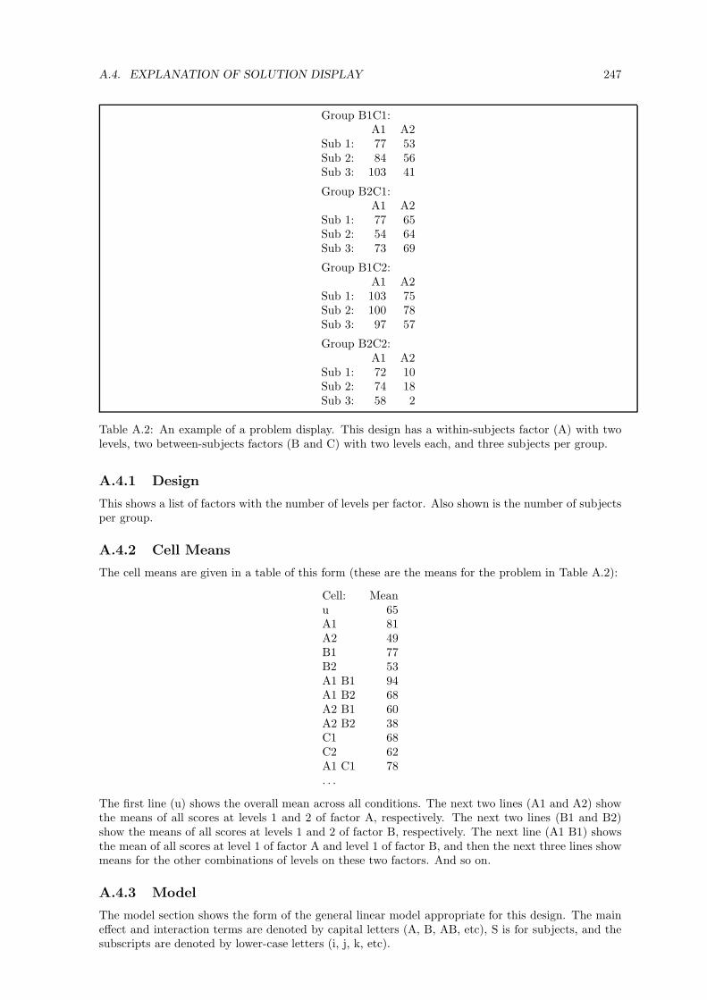
A.4. EXPLANATION OF SOLUTION DISPLAY 247
Group B1C1:A1 A2
Sub 1: 77 53Sub 2: 84 56Sub 3: 103 41
Group B2C1:A1 A2
Sub 1: 77 65Sub 2: 54 64Sub 3: 73 69
Group B1C2:A1 A2
Sub 1: 103 75Sub 2: 100 78Sub 3: 97 57
Group B2C2:A1 A2
Sub 1: 72 10Sub 2: 74 18Sub 3: 58 2
Table A.2: An example of a problem display. This design has a within-subjects factor (A) with twolevels, two between-subjects factors (B and C) with two levels each, and three subjects per group.
A.4.1 Design
This shows a list of factors with the number of levels per factor. Also shown is the number of subjectsper group.
A.4.2 Cell Means
The cell means are given in a table of this form (these are the means for the problem in Table A.2):
Cell: Meanu 65A1 81A2 49B1 77B2 53A1 B1 94A1 B2 68A2 B1 60A2 B2 38C1 68C2 62A1 C1 78. . .
The first line (u) shows the overall mean across all conditions. The next two lines (A1 and A2) showthe means of all scores at levels 1 and 2 of factor A, respectively. The next two lines (B1 and B2)show the means of all scores at levels 1 and 2 of factor B, respectively. The next line (A1 B1) showsthe mean of all scores at level 1 of factor A and level 1 of factor B, and then the next three lines showmeans for the other combinations of levels on these two factors. And so on.
A.4.3 Model
The model section shows the form of the general linear model appropriate for this design. The maineffect and interaction terms are denoted by capital letters (A, B, AB, etc), S is for subjects, and thesubscripts are denoted by lower-case letters (i, j, k, etc).

248 APPENDIX A. THE ANOGEN PROGRAM
A.4.4 Estimation Equations
The estimation equations section shows the equation used to estimate each term in the linear model.The period subscript is used to denote averaging across levels of the factor corresponding to thatsubscript.
A.4.5 Decomposition Matrix
The decomposition matrix shows the breakdown of all data values (numbers of the left sides of theequals signs) into the estimated values corresponding to each term in the linear model. The order ofthe numbers on the line is the same as the order of the terms in the model.
A.4.6 ANOVA Table
The ANOVA table is in a relatively standard format. The F value is marked with one asterisk if it issignificant at the level of p < .05 and two asterisks if significant at p < .01. The error term used tocompute each F is shown at the far right side of the table.

Appendix B
Statistical Tables
249

250 APPENDIX B. STATISTICAL TABLES
B.1 F -Critical Values
The following six pages give tables of F -critical values for p = .10, p = .05, p = .025, p = .01, p = .005,and p = .001, respectively. The most “standard” values are those with p = .05.

B.1. F -CRITICAL VALUES 251F-C
riti
calV
alu
esfo
rp
=.1
0D
FE
rror
Deg
rees
ofFre
edom
for
Effec
t,In
tera
ctio
n,et
c(N
um
erato
r)(D
enom
)1
23
45
67
89
10
12
15
20
24
30
40
60
120
250
139.8
63
49.5
00
53.5
93
55.8
33
57.2
40
58.2
04
58.9
06
59.4
39
59.8
58
60.1
95
60.7
05
61.2
20
61.7
40
62.0
02
62.2
65
62.5
29
62.7
94
63.0
61
63.2
03
28.5
26
9.0
00
9.1
62
9.2
43
9.2
93
9.3
26
9.3
49
9.3
67
9.3
81
9.3
92
9.4
08
9.4
25
9.4
41
9.4
50
9.4
58
9.4
66
9.4
75
9.4
83
9.4
87
35.5
38
5.4
62
5.3
91
5.3
43
5.3
09
5.2
85
5.2
66
5.2
52
5.2
40
5.2
30
5.2
16
5.2
00
5.1
84
5.1
76
5.1
68
5.1
60
5.1
51
5.1
43
5.1
38
44.5
45
4.3
25
4.1
91
4.1
07
4.0
51
4.0
10
3.9
79
3.9
55
3.9
36
3.9
20
3.8
96
3.8
70
3.8
44
3.8
31
3.8
17
3.8
04
3.7
90
3.7
75
3.7
68
54.0
60
3.7
80
3.6
19
3.5
20
3.4
53
3.4
05
3.3
68
3.3
39
3.3
16
3.2
97
3.2
68
3.2
38
3.2
07
3.1
91
3.1
74
3.1
57
3.1
40
3.1
23
3.1
14
63.7
76
3.4
63
3.2
89
3.1
81
3.1
08
3.0
55
3.0
14
2.9
83
2.9
58
2.9
37
2.9
05
2.8
71
2.8
36
2.8
18
2.8
00
2.7
81
2.7
62
2.7
42
2.7
32
73.5
89
3.2
57
3.0
74
2.9
61
2.8
83
2.8
27
2.7
85
2.7
52
2.7
25
2.7
03
2.6
68
2.6
32
2.5
95
2.5
75
2.5
55
2.5
35
2.5
14
2.4
93
2.4
81
83.4
58
3.1
13
2.9
24
2.8
06
2.7
26
2.6
68
2.6
24
2.5
89
2.5
61
2.5
38
2.5
02
2.4
64
2.4
25
2.4
04
2.3
83
2.3
61
2.3
39
2.3
16
2.3
04
93.3
60
3.0
06
2.8
13
2.6
93
2.6
11
2.5
51
2.5
05
2.4
69
2.4
40
2.4
16
2.3
79
2.3
40
2.2
98
2.2
77
2.2
55
2.2
32
2.2
08
2.1
84
2.1
71
10
3.2
85
2.9
24
2.7
28
2.6
05
2.5
22
2.4
61
2.4
14
2.3
77
2.3
47
2.3
23
2.2
84
2.2
44
2.2
01
2.1
78
2.1
55
2.1
32
2.1
07
2.0
82
2.0
68
11
3.2
25
2.8
60
2.6
60
2.5
36
2.4
51
2.3
89
2.3
42
2.3
04
2.2
74
2.2
48
2.2
09
2.1
67
2.1
23
2.1
00
2.0
76
2.0
52
2.0
26
2.0
00
1.9
85
12
3.1
77
2.8
07
2.6
06
2.4
80
2.3
94
2.3
31
2.2
83
2.2
45
2.2
14
2.1
88
2.1
47
2.1
05
2.0
60
2.0
36
2.0
11
1.9
86
1.9
60
1.9
32
1.9
18
13
3.1
36
2.7
63
2.5
60
2.4
34
2.3
47
2.2
83
2.2
34
2.1
95
2.1
64
2.1
38
2.0
97
2.0
53
2.0
07
1.9
83
1.9
58
1.9
31
1.9
04
1.8
76
1.8
61
14
3.1
02
2.7
26
2.5
22
2.3
95
2.3
07
2.2
43
2.1
93
2.1
54
2.1
22
2.0
95
2.0
54
2.0
10
1.9
62
1.9
38
1.9
12
1.8
85
1.8
57
1.8
28
1.8
12
15
3.0
73
2.6
95
2.4
90
2.3
61
2.2
73
2.2
08
2.1
58
2.1
19
2.0
86
2.0
59
2.0
17
1.9
72
1.9
24
1.8
99
1.8
73
1.8
45
1.8
17
1.7
87
1.7
70
16
3.0
48
2.6
68
2.4
62
2.3
33
2.2
44
2.1
78
2.1
28
2.0
88
2.0
55
2.0
28
1.9
85
1.9
40
1.8
91
1.8
66
1.8
39
1.8
11
1.7
82
1.7
51
1.7
34
17
3.0
26
2.6
45
2.4
37
2.3
08
2.2
18
2.1
52
2.1
02
2.0
61
2.0
28
2.0
01
1.9
58
1.9
12
1.8
62
1.8
36
1.8
09
1.7
81
1.7
51
1.7
19
1.7
02
18
3.0
07
2.6
24
2.4
16
2.2
86
2.1
96
2.1
30
2.0
79
2.0
38
2.0
05
1.9
77
1.9
33
1.8
87
1.8
37
1.8
10
1.7
83
1.7
54
1.7
23
1.6
91
1.6
73
19
2.9
90
2.6
06
2.3
97
2.2
66
2.1
76
2.1
09
2.0
58
2.0
17
1.9
84
1.9
56
1.9
12
1.8
65
1.8
14
1.7
87
1.7
59
1.7
30
1.6
99
1.6
66
1.6
48
20
2.9
75
2.5
89
2.3
80
2.2
49
2.1
58
2.0
91
2.0
40
1.9
99
1.9
65
1.9
37
1.8
92
1.8
45
1.7
94
1.7
67
1.7
38
1.7
08
1.6
77
1.6
43
1.6
25
21
2.9
61
2.5
75
2.3
65
2.2
33
2.1
42
2.0
75
2.0
23
1.9
82
1.9
48
1.9
20
1.8
75
1.8
27
1.7
76
1.7
48
1.7
19
1.6
89
1.6
57
1.6
23
1.6
04
22
2.9
49
2.5
61
2.3
51
2.2
19
2.1
28
2.0
60
2.0
08
1.9
67
1.9
33
1.9
04
1.8
59
1.8
11
1.7
59
1.7
31
1.7
02
1.6
71
1.6
39
1.6
04
1.5
85
23
2.9
37
2.5
49
2.3
39
2.2
07
2.1
15
2.0
47
1.9
95
1.9
53
1.9
19
1.8
90
1.8
45
1.7
96
1.7
44
1.7
16
1.6
86
1.6
55
1.6
22
1.5
87
1.5
68
24
2.9
27
2.5
38
2.3
27
2.1
95
2.1
03
2.0
35
1.9
83
1.9
41
1.9
06
1.8
77
1.8
32
1.7
83
1.7
30
1.7
02
1.6
72
1.6
41
1.6
07
1.5
71
1.5
52
25
2.9
18
2.5
28
2.3
17
2.1
84
2.0
92
2.0
24
1.9
71
1.9
29
1.8
95
1.8
66
1.8
20
1.7
71
1.7
18
1.6
89
1.6
59
1.6
27
1.5
93
1.5
57
1.5
37
26
2.9
09
2.5
19
2.3
07
2.1
74
2.0
82
2.0
14
1.9
61
1.9
19
1.8
84
1.8
55
1.8
09
1.7
60
1.7
06
1.6
77
1.6
47
1.6
15
1.5
81
1.5
44
1.5
23
27
2.9
01
2.5
11
2.2
99
2.1
65
2.0
73
2.0
05
1.9
52
1.9
09
1.8
74
1.8
45
1.7
99
1.7
49
1.6
95
1.6
66
1.6
36
1.6
03
1.5
69
1.5
31
1.5
11
28
2.8
94
2.5
03
2.2
91
2.1
57
2.0
64
1.9
96
1.9
43
1.9
00
1.8
65
1.8
36
1.7
90
1.7
40
1.6
85
1.6
56
1.6
25
1.5
92
1.5
58
1.5
20
1.4
99
29
2.8
87
2.4
95
2.2
83
2.1
49
2.0
57
1.9
88
1.9
35
1.8
92
1.8
57
1.8
27
1.7
81
1.7
31
1.6
76
1.6
47
1.6
16
1.5
83
1.5
47
1.5
09
1.4
88
30
2.8
81
2.4
89
2.2
76
2.1
42
2.0
49
1.9
80
1.9
27
1.8
84
1.8
49
1.8
19
1.7
73
1.7
22
1.6
67
1.6
38
1.6
06
1.5
73
1.5
38
1.4
99
1.4
77
40
2.8
35
2.4
40
2.2
26
2.0
91
1.9
97
1.9
27
1.8
73
1.8
29
1.7
93
1.7
63
1.7
15
1.6
62
1.6
05
1.5
74
1.5
41
1.5
06
1.4
67
1.4
25
1.4
01
60
2.7
91
2.3
93
2.1
77
2.0
41
1.9
46
1.8
75
1.8
19
1.7
75
1.7
38
1.7
07
1.6
57
1.6
03
1.5
43
1.5
11
1.4
76
1.4
37
1.3
95
1.3
48
1.3
20
120
2.7
48
2.3
47
2.1
30
1.9
92
1.8
96
1.8
24
1.7
67
1.7
22
1.6
84
1.6
52
1.6
01
1.5
45
1.4
82
1.4
47
1.4
09
1.3
68
1.3
20
1.2
65
1.2
30
250
2.7
26
2.3
24
2.1
06
1.9
67
1.8
70
1.7
98
1.7
41
1.6
95
1.6
57
1.6
24
1.5
72
1.5
15
1.4
50
1.4
14
1.3
75
1.3
30
1.2
79
1.2
17
1.1
76
Note
:If
this
table
does
not
incl
ude
the
valu
eofD
FE
rror
that
you
want,
you
should
eith
erget
am
ore
com
ple
teta
ble
or
else
use
the
nex
tsm
aller
DF
Err
or
valu
ein
this
table
.

252 APPENDIX B. STATISTICAL TABLESF-C
riticalV
alu
esfo
rp
=.0
5D
FE
rror
Deg
reesofFreed
om
for
Effect,
Intera
ction,etc
(Num
erato
r)(D
enom
)1
23
45
67
89
10
12
15
20
24
30
40
60
120
250
1161.4
5199.5
0215.7
1224.5
8230.1
6233.9
9236.7
7238.8
8240.5
4241.8
8243.9
1245.9
5248.0
1249.0
5250.1
0251.1
4252.2
0253.2
5253.8
02
18.5
119.0
019.1
619.2
519.3
019.3
319.3
519.3
719.3
819.4
019.4
119.4
319.4
519.4
519.4
619.4
719.4
819.4
919.4
93
10.1
39.5
59.2
89.1
29.0
18.9
48.8
98.8
58.8
18.7
98.7
48.7
08.6
68.6
48.6
28.5
98.5
78.5
58.5
44
7.7
16.9
46.5
96.3
96.2
66.1
66.0
96.0
46.0
05.9
65.9
15.8
65.8
05.7
75.7
55.7
25.6
95.6
65.6
45
6.6
15.7
95.4
15.1
95.0
54.9
54.8
84.8
24.7
74.7
44.6
84.6
24.5
64.5
34.5
04.4
64.4
34.4
04.3
8
65.9
95.1
44.7
64.5
34.3
94.2
84.2
14.1
54.1
04.0
64.0
03.9
43.8
73.8
43.8
13.7
73.7
43.7
03.6
97
5.5
94.7
44.3
54.1
23.9
73.8
73.7
93.7
33.6
83.6
43.5
73.5
13.4
43.4
13.3
83.3
43.3
03.2
73.2
58
5.3
24.4
64.0
73.8
43.6
93.5
83.5
03.4
43.3
93.3
53.2
83.2
23.1
53.1
23.0
83.0
43.0
12.9
72.9
59
5.1
24.2
63.8
63.6
33.4
83.3
73.2
93.2
33.1
83.1
43.0
73.0
12.9
42.9
02.8
62.8
32.7
92.7
52.7
310
4.9
64.1
03.7
13.4
83.3
33.2
23.1
43.0
73.0
22.9
82.9
12.8
52.7
72.7
42.7
02.6
62.6
22.5
82.5
6
11
4.8
43.9
83.5
93.3
63.2
03.0
93.0
12.9
52.9
02.8
52.7
92.7
22.6
52.6
12.5
72.5
32.4
92.4
52.4
312
4.7
53.8
93.4
93.2
63.1
13.0
02.9
12.8
52.8
02.7
52.6
92.6
22.5
42.5
12.4
72.4
32.3
82.3
42.3
213
4.6
73.8
13.4
13.1
83.0
32.9
22.8
32.7
72.7
12.6
72.6
02.5
32.4
62.4
22.3
82.3
42.3
02.2
52.2
314
4.6
03.7
43.3
43.1
12.9
62.8
52.7
62.7
02.6
52.6
02.5
32.4
62.3
92.3
52.3
12.2
72.2
22.1
82.1
515
4.5
43.6
83.2
93.0
62.9
02.7
92.7
12.6
42.5
92.5
42.4
82.4
02.3
32.2
92.2
52.2
02.1
62.1
12.0
9
16
4.4
93.6
33.2
43.0
12.8
52.7
42.6
62.5
92.5
42.4
92.4
22.3
52.2
82.2
42.1
92.1
52.1
12.0
62.0
317
4.4
53.5
93.2
02.9
62.8
12.7
02.6
12.5
52.4
92.4
52.3
82.3
12.2
32.1
92.1
52.1
02.0
62.0
11.9
818
4.4
13.5
53.1
62.9
32.7
72.6
62.5
82.5
12.4
62.4
12.3
42.2
72.1
92.1
52.1
12.0
62.0
21.9
71.9
419
4.3
83.5
23.1
32.9
02.7
42.6
32.5
42.4
82.4
22.3
82.3
12.2
32.1
62.1
12.0
72.0
31.9
81.9
31.9
020
4.3
53.4
93.1
02.8
72.7
12.6
02.5
12.4
52.3
92.3
52.2
82.2
02.1
22.0
82.0
41.9
91.9
51.9
01.8
7
21
4.3
23.4
73.0
72.8
42.6
82.5
72.4
92.4
22.3
72.3
22.2
52.1
82.1
02.0
52.0
11.9
61.9
21.8
71.8
422
4.3
03.4
43.0
52.8
22.6
62.5
52.4
62.4
02.3
42.3
02.2
32.1
52.0
72.0
31.9
81.9
41.8
91.8
41.8
123
4.2
83.4
23.0
32.8
02.6
42.5
32.4
42.3
72.3
22.2
72.2
02.1
32.0
52.0
11.9
61.9
11.8
61.8
11.7
824
4.2
63.4
03.0
12.7
82.6
22.5
12.4
22.3
62.3
02.2
52.1
82.1
12.0
31.9
81.9
41.8
91.8
41.7
91.7
625
4.2
43.3
92.9
92.7
62.6
02.4
92.4
02.3
42.2
82.2
42.1
62.0
92.0
11.9
61.9
21.8
71.8
21.7
71.7
4
26
4.2
33.3
72.9
82.7
42.5
92.4
72.3
92.3
22.2
72.2
22.1
52.0
71.9
91.9
51.9
01.8
51.8
01.7
51.7
227
4.2
13.3
52.9
62.7
32.5
72.4
62.3
72.3
12.2
52.2
02.1
32.0
61.9
71.9
31.8
81.8
41.7
91.7
31.7
028
4.2
03.3
42.9
52.7
12.5
62.4
52.3
62.2
92.2
42.1
92.1
22.0
41.9
61.9
11.8
71.8
21.7
71.7
11.6
829
4.1
83.3
32.9
32.7
02.5
52.4
32.3
52.2
82.2
22.1
82.1
02.0
31.9
41.9
01.8
51.8
11.7
51.7
01.6
730
4.1
73.3
22.9
22.6
92.5
32.4
22.3
32.2
72.2
12.1
62.0
92.0
11.9
31.8
91.8
41.7
91.7
41.6
81.6
5
40
4.0
83.2
32.8
42.6
12.4
52.3
42.2
52.1
82.1
22.0
82.0
01.9
21.8
41.7
91.7
41.6
91.6
41.5
81.5
460
4.0
03.1
52.7
62.5
32.3
72.2
52.1
72.1
02.0
41.9
91.9
21.8
41.7
51.7
01.6
51.5
91.5
31.4
71.4
3120
3.9
23.0
72.6
82.4
52.2
92.1
82.0
92.0
21.9
61.9
11.8
31.7
51.6
61.6
11.5
51.5
01.4
31.3
51.3
0250
3.8
83.0
32.6
42.4
12.2
52.1
32.0
51.9
81.9
21.8
71.7
91.7
11.6
11.5
61.5
01.4
41.3
71.2
91.2
3
Note:
Ifth
ista
ble
does
not
inclu
de
the
valu
eofD
FE
rror
that
you
want,
you
should
either
get
am
ore
com
plete
table
or
elseuse
the
nex
tsm
aller
DF
Erro
rva
lue
inth
ista
ble.

B.1. F -CRITICAL VALUES 253F-C
riti
calV
alu
esfo
rp
=.0
25
DF
Err
or
Deg
rees
ofFre
edom
for
Effec
t,In
tera
ctio
n,et
c(N
um
erato
r)(D
enom
)1
23
45
67
89
10
12
15
20
24
30
40
60
120
250
1647.7
9799.5
0864.1
6899.5
8921.8
5937.1
1948.2
2956.6
6963.2
8968.6
3976.7
1984.8
7993.1
0997.2
51001.4
11005.6
01009.8
01014.0
21016.2
22
38.5
139.0
039.1
739.2
539.3
039.3
339.3
639.3
739.3
939.4
039.4
139.4
339.4
539.4
639.4
639.4
739.4
839.4
939.4
93
17.4
416.0
415.4
415.1
014.8
914.7
314.6
214.5
414.4
714.4
214.3
414.2
514.1
714.1
214.0
814.0
413.9
913.9
513.9
24
12.2
210.6
59.9
89.6
09.3
69.2
09.0
78.9
88.9
08.8
48.7
58.6
68.5
68.5
18.4
68.4
18.3
68.3
18.2
85
10.0
18.4
37.7
67.3
97.1
56.9
86.8
56.7
66.6
86.6
26.5
26.4
36.3
36.2
86.2
36.1
86.1
26.0
76.0
4
68.8
17.2
66.6
06.2
35.9
95.8
25.7
05.6
05.5
25.4
65.3
75.2
75.1
75.1
25.0
75.0
14.9
64.9
04.8
87
8.0
76.5
45.8
95.5
25.2
95.1
24.9
94.9
04.8
24.7
64.6
74.5
74.4
74.4
14.3
64.3
14.2
54.2
04.1
78
7.5
76.0
65.4
25.0
54.8
24.6
54.5
34.4
34.3
64.3
04.2
04.1
04.0
03.9
53.8
93.8
43.7
83.7
33.7
09
7.2
15.7
15.0
84.7
24.4
84.3
24.2
04.1
04.0
33.9
63.8
73.7
73.6
73.6
13.5
63.5
13.4
53.3
93.3
610
6.9
45.4
64.8
34.4
74.2
44.0
73.9
53.8
53.7
83.7
23.6
23.5
23.4
23.3
73.3
13.2
63.2
03.1
43.1
1
11
6.7
25.2
64.6
34.2
84.0
43.8
83.7
63.6
63.5
93.5
33.4
33.3
33.2
33.1
73.1
23.0
63.0
02.9
42.9
112
6.5
55.1
04.4
74.1
23.8
93.7
33.6
13.5
13.4
43.3
73.2
83.1
83.0
73.0
22.9
62.9
12.8
52.7
92.7
613
6.4
14.9
74.3
54.0
03.7
73.6
03.4
83.3
93.3
13.2
53.1
53.0
52.9
52.8
92.8
42.7
82.7
22.6
62.6
314
6.3
04.8
64.2
43.8
93.6
63.5
03.3
83.2
93.2
13.1
53.0
52.9
52.8
42.7
92.7
32.6
72.6
12.5
52.5
215
6.2
04.7
74.1
53.8
03.5
83.4
13.2
93.2
03.1
23.0
62.9
62.8
62.7
62.7
02.6
42.5
92.5
22.4
62.4
3
16
6.1
24.6
94.0
83.7
33.5
03.3
43.2
23.1
23.0
52.9
92.8
92.7
92.6
82.6
32.5
72.5
12.4
52.3
82.3
517
6.0
44.6
24.0
13.6
63.4
43.2
83.1
63.0
62.9
82.9
22.8
22.7
22.6
22.5
62.5
02.4
42.3
82.3
22.2
818
5.9
84.5
63.9
53.6
13.3
83.2
23.1
03.0
12.9
32.8
72.7
72.6
72.5
62.5
02.4
42.3
82.3
22.2
62.2
219
5.9
24.5
13.9
03.5
63.3
33.1
73.0
52.9
62.8
82.8
22.7
22.6
22.5
12.4
52.3
92.3
32.2
72.2
02.1
720
5.8
74.4
63.8
63.5
13.2
93.1
33.0
12.9
12.8
42.7
72.6
82.5
72.4
62.4
12.3
52.2
92.2
22.1
62.1
2
21
5.8
34.4
23.8
23.4
83.2
53.0
92.9
72.8
72.8
02.7
32.6
42.5
32.4
22.3
72.3
12.2
52.1
82.1
12.0
822
5.7
94.3
83.7
83.4
43.2
23.0
52.9
32.8
42.7
62.7
02.6
02.5
02.3
92.3
32.2
72.2
12.1
42.0
82.0
423
5.7
54.3
53.7
53.4
13.1
83.0
22.9
02.8
12.7
32.6
72.5
72.4
72.3
62.3
02.2
42.1
82.1
12.0
42.0
024
5.7
24.3
23.7
23.3
83.1
52.9
92.8
72.7
82.7
02.6
42.5
42.4
42.3
32.2
72.2
12.1
52.0
82.0
11.9
725
5.6
94.2
93.6
93.3
53.1
32.9
72.8
52.7
52.6
82.6
12.5
12.4
12.3
02.2
42.1
82.1
22.0
51.9
81.9
4
26
5.6
64.2
73.6
73.3
33.1
02.9
42.8
22.7
32.6
52.5
92.4
92.3
92.2
82.2
22.1
62.0
92.0
31.9
51.9
227
5.6
34.2
43.6
53.3
13.0
82.9
22.8
02.7
12.6
32.5
72.4
72.3
62.2
52.1
92.1
32.0
72.0
01.9
31.8
928
5.6
14.2
23.6
33.2
93.0
62.9
02.7
82.6
92.6
12.5
52.4
52.3
42.2
32.1
72.1
12.0
51.9
81.9
11.8
729
5.5
94.2
03.6
13.2
73.0
42.8
82.7
62.6
72.5
92.5
32.4
32.3
22.2
12.1
52.0
92.0
31.9
61.8
91.8
530
5.5
74.1
83.5
93.2
53.0
32.8
72.7
52.6
52.5
72.5
12.4
12.3
12.2
02.1
42.0
72.0
11.9
41.8
71.8
3
40
5.4
24.0
53.4
63.1
32.9
02.7
42.6
22.5
32.4
52.3
92.2
92.1
82.0
72.0
11.9
41.8
81.8
01.7
21.6
860
5.2
93.9
33.3
43.0
12.7
92.6
32.5
12.4
12.3
32.2
72.1
72.0
61.9
41.8
81.8
21.7
41.6
71.5
81.5
3120
5.1
53.8
03.2
32.8
92.6
72.5
22.3
92.3
02.2
22.1
62.0
51.9
41.8
21.7
61.6
91.6
11.5
31.4
31.3
7250
5.0
83.7
43.1
72.8
42.6
22.4
62.3
42.2
42.1
62.1
02.0
01.8
91.7
61.7
01.6
31.5
51.4
61.3
51.2
8500
5.0
53.7
23.1
42.8
12.5
92.4
32.3
12.2
22.1
42.0
71.9
71.8
61.7
41.6
71.6
01.5
21.4
21.3
11.2
4
Note
:If
this
table
does
not
incl
ude
the
valu
eofD
FE
rror
that
you
want,
you
should
eith
erget
am
ore
com
ple
teta
ble
or
else
use
the
nex
tsm
aller
DF
Err
or
valu
ein
this
table
.

254 APPENDIX B. STATISTICAL TABLES
F-C
riticalV
alu
esfo
rp
=.0
1D
FE
rror
Deg
reesofFreed
om
for
Effect,
Intera
ction,etc
(Num
erato
r)(D
enom
)1
23
45
67
89
10
12
15
20
24
30
40
60
120
250
14052.2
4999.5
5403.3
5624.6
5763.6
5859.0
5928.4
5981.1
6022.5
6055.8
6106.3
6157.3
6208.7
6234.6
6260.6
6286.8
6313.0
6339.4
6353.1
298.5
099.0
099.1
799.2
599.3
099.3
399.3
699.3
799.3
999.4
099.4
299.4
399.4
599.4
699.4
799.4
799.4
899.4
999.5
03
34.1
230.8
229.4
628.7
128.2
427.9
127.6
727.4
927.3
527.2
327.0
526.8
726.6
926.6
026.5
026.4
126.3
226.2
226.1
74
21.2
018.0
016.6
915.9
815.5
215.2
114.9
814.8
014.6
614.5
514.3
714.2
014.0
213.9
313.8
413.7
513.6
513.5
613.5
15
16.2
613.2
712.0
611.3
910.9
710.6
710.4
610.2
910.1
610.0
59.8
99.7
29.5
59.4
79.3
89.2
99.2
09.1
19.0
6
613.7
510.9
29.7
89.1
58.7
58.4
78.2
68.1
07.9
87.8
77.7
27.5
67.4
07.3
17.2
37.1
47.0
66.9
76.9
27
12.2
59.5
58.4
57.8
57.4
67.1
96.9
96.8
46.7
26.6
26.4
76.3
16.1
66.0
75.9
95.9
15.8
25.7
45.6
98
11.2
68.6
57.5
97.0
16.6
36.3
76.1
86.0
35.9
15.8
15.6
75.5
25.3
65.2
85.2
05.1
25.0
34.9
54.9
09
10.5
68.0
26.9
96.4
26.0
65.8
05.6
15.4
75.3
55.2
65.1
14.9
64.8
14.7
34.6
54.5
74.4
84.4
04.3
510
10.0
47.5
66.5
55.9
95.6
45.3
95.2
05.0
64.9
44.8
54.7
14.5
64.4
14.3
34.2
54.1
74.0
84.0
03.9
5
11
9.6
57.2
16.2
25.6
75.3
25.0
74.8
94.7
44.6
34.5
44.4
04.2
54.1
04.0
23.9
43.8
63.7
83.6
93.6
412
9.3
36.9
35.9
55.4
15.0
64.8
24.6
44.5
04.3
94.3
04.1
64.0
13.8
63.7
83.7
03.6
23.5
43.4
53.4
013
9.0
76.7
05.7
45.2
14.8
64.6
24.4
44.3
04.1
94.1
03.9
63.8
23.6
63.5
93.5
13.4
33.3
43.2
53.2
114
8.8
66.5
15.5
65.0
44.6
94.4
64.2
84.1
44.0
33.9
43.8
03.6
63.5
13.4
33.3
53.2
73.1
83.0
93.0
515
8.6
86.3
65.4
24.8
94.5
64.3
24.1
44.0
03.8
93.8
03.6
73.5
23.3
73.2
93.2
13.1
33.0
52.9
62.9
1
16
8.5
36.2
35.2
94.7
74.4
44.2
04.0
33.8
93.7
83.6
93.5
53.4
13.2
63.1
83.1
03.0
22.9
32.8
42.8
017
8.4
06.1
15.1
84.6
74.3
44.1
03.9
33.7
93.6
83.5
93.4
63.3
13.1
63.0
83.0
02.9
22.8
32.7
52.7
018
8.2
96.0
15.0
94.5
84.2
54.0
13.8
43.7
13.6
03.5
13.3
73.2
33.0
83.0
02.9
22.8
42.7
52.6
62.6
119
8.1
85.9
35.0
14.5
04.1
73.9
43.7
73.6
33.5
23.4
33.3
03.1
53.0
02.9
22.8
42.7
62.6
72.5
82.5
420
8.1
05.8
54.9
44.4
34.1
03.8
73.7
03.5
63.4
63.3
73.2
33.0
92.9
42.8
62.7
82.6
92.6
12.5
22.4
7
21
8.0
25.7
84.8
74.3
74.0
43.8
13.6
43.5
13.4
03.3
13.1
73.0
32.8
82.8
02.7
22.6
42.5
52.4
62.4
122
7.9
55.7
24.8
24.3
13.9
93.7
63.5
93.4
53.3
53.2
63.1
22.9
82.8
32.7
52.6
72.5
82.5
02.4
02.3
523
7.8
85.6
64.7
64.2
63.9
43.7
13.5
43.4
13.3
03.2
13.0
72.9
32.7
82.7
02.6
22.5
42.4
52.3
52.3
024
7.8
25.6
14.7
24.2
23.9
03.6
73.5
03.3
63.2
63.1
73.0
32.8
92.7
42.6
62.5
82.4
92.4
02.3
12.2
625
7.7
75.5
74.6
84.1
83.8
53.6
33.4
63.3
23.2
23.1
32.9
92.8
52.7
02.6
22.5
42.4
52.3
62.2
72.2
2
26
7.7
25.5
34.6
44.1
43.8
23.5
93.4
23.2
93.1
83.0
92.9
62.8
12.6
62.5
82.5
02.4
22.3
32.2
32.1
827
7.6
85.4
94.6
04.1
13.7
83.5
63.3
93.2
63.1
53.0
62.9
32.7
82.6
32.5
52.4
72.3
82.2
92.2
02.1
528
7.6
45.4
54.5
74.0
73.7
53.5
33.3
63.2
33.1
23.0
32.9
02.7
52.6
02.5
22.4
42.3
52.2
62.1
72.1
129
7.6
05.4
24.5
44.0
43.7
33.5
03.3
33.2
03.0
93.0
02.8
72.7
32.5
72.4
92.4
12.3
32.2
32.1
42.0
830
7.5
65.3
94.5
14.0
23.7
03.4
73.3
03.1
73.0
72.9
82.8
42.7
02.5
52.4
72.3
92.3
02.2
12.1
12.0
6
40
7.3
15.1
84.3
13.8
33.5
13.2
93.1
22.9
92.8
92.8
02.6
62.5
22.3
72.2
92.2
02.1
12.0
21.9
21.8
660
7.0
84.9
84.1
33.6
53.3
43.1
22.9
52.8
22.7
22.6
32.5
02.3
52.2
02.1
22.0
31.9
41.8
41.7
31.6
6120
6.8
54.7
93.9
53.4
83.1
72.9
62.7
92.6
62.5
62.4
72.3
42.1
92.0
31.9
51.8
61.7
61.6
61.5
31.4
6250
6.7
44.6
93.8
63.4
03.0
92.8
72.7
12.5
82.4
82.3
92.2
62.1
11.9
51.8
71.7
71.6
71.5
61.4
31.3
4500
6.6
94.6
53.8
23.3
63.0
52.8
42.6
82.5
52.4
42.3
62.2
22.0
71.9
21.8
31.7
41.6
31.5
21.3
81.2
8
Note:
Ifth
ista
ble
does
not
inclu
de
the
valu
eofD
FE
rror
that
you
want,
you
should
either
get
am
ore
com
plete
table
or
elseuse
the
nex
tsm
aller
DF
Erro
rva
lue
inth
ista
ble.

B.1. F -CRITICAL VALUES 255F-C
riti
calV
alu
esfo
rp
=.0
05
DF
Err
or
Deg
rees
ofFre
edom
for
Effec
t,In
tera
ctio
n,et
c(N
um
erato
r)(D
enom
)1
23
45
67
89
10
12
15
20
24
30
40
60
120
250
1Too
Big
for
my
Com
pute
r!2
198.5
0199.0
0199.1
7199.2
5199.3
0199.3
3199.3
6199.3
7199.3
9199.4
0199.4
2199.4
3199.4
5199.4
6199.4
7199.4
7199.4
8199.4
9199.5
03
55.5
549.8
047.4
746.1
945.3
944.8
444.4
344.1
343.8
843.6
943.3
943.0
842.7
842.6
242.4
742.3
142.1
541.9
941.9
14
31.3
326.2
824.2
623.1
522.4
621.9
721.6
221.3
521.1
420.9
720.7
020.4
420.1
720.0
319.8
919.7
519.6
119.4
719.3
95
22.7
818.3
116.5
315.5
614.9
414.5
114.2
013.9
613.7
713.6
213.3
813.1
512.9
012.7
812.6
612.5
312.4
012.2
712.2
1
618.6
414.5
412.9
212.0
311.4
611.0
710.7
910.5
710.3
910.2
510.0
39.8
19.5
99.4
79.3
69.2
49.1
29.0
08.9
47
16.2
412.4
010.8
810.0
59.5
29.1
68.8
98.6
88.5
18.3
88.1
87.9
77.7
57.6
47.5
37.4
27.3
17.1
97.1
38
14.6
911.0
49.6
08.8
18.3
07.9
57.6
97.5
07.3
47.2
17.0
16.8
16.6
16.5
06.4
06.2
96.1
86.0
66.0
19
13.6
110.1
18.7
27.9
67.4
77.1
36.8
86.6
96.5
46.4
26.2
36.0
35.8
35.7
35.6
25.5
25.4
15.3
05.2
410
12.8
39.4
38.0
87.3
46.8
76.5
46.3
06.1
25.9
75.8
55.6
65.4
75.2
75.1
75.0
74.9
74.8
64.7
54.6
9
11
12.2
38.9
17.6
06.8
86.4
26.1
05.8
65.6
85.5
45.4
25.2
45.0
54.8
64.7
64.6
54.5
54.4
54.3
44.2
812
11.7
58.5
17.2
36.5
26.0
75.7
65.5
25.3
55.2
05.0
94.9
14.7
24.5
34.4
34.3
34.2
34.1
24.0
13.9
613
11.3
78.1
96.9
36.2
35.7
95.4
85.2
55.0
84.9
44.8
24.6
44.4
64.2
74.1
74.0
73.9
73.8
73.7
63.7
014
11.0
67.9
26.6
86.0
05.5
65.2
65.0
34.8
64.7
24.6
04.4
34.2
54.0
63.9
63.8
63.7
63.6
63.5
53.4
915
10.8
07.7
06.4
85.8
05.3
75.0
74.8
54.6
74.5
44.4
24.2
54.0
73.8
83.7
93.6
93.5
83.4
83.3
73.3
1
16
10.5
87.5
16.3
05.6
45.2
14.9
14.6
94.5
24.3
84.2
74.1
03.9
23.7
33.6
43.5
43.4
43.3
33.2
23.1
717
10.3
87.3
56.1
65.5
05.0
74.7
84.5
64.3
94.2
54.1
43.9
73.7
93.6
13.5
13.4
13.3
13.2
13.1
03.0
418
10.2
27.2
16.0
35.3
74.9
64.6
64.4
44.2
84.1
44.0
33.8
63.6
83.5
03.4
03.3
03.2
03.1
02.9
92.9
319
10.0
77.0
95.9
25.2
74.8
54.5
64.3
44.1
84.0
43.9
33.7
63.5
93.4
03.3
13.2
13.1
13.0
02.8
92.8
320
9.9
46.9
95.8
25.1
74.7
64.4
74.2
64.0
93.9
63.8
53.6
83.5
03.3
23.2
23.1
23.0
22.9
22.8
12.7
5
21
9.8
36.8
95.7
35.0
94.6
84.3
94.1
84.0
13.8
83.7
73.6
03.4
33.2
43.1
53.0
52.9
52.8
42.7
32.6
722
9.7
36.8
15.6
55.0
24.6
14.3
24.1
13.9
43.8
13.7
03.5
43.3
63.1
83.0
82.9
82.8
82.7
72.6
62.6
023
9.6
36.7
35.5
84.9
54.5
44.2
64.0
53.8
83.7
53.6
43.4
73.3
03.1
23.0
22.9
22.8
22.7
12.6
02.5
424
9.5
56.6
65.5
24.8
94.4
94.2
03.9
93.8
33.6
93.5
93.4
23.2
53.0
62.9
72.8
72.7
72.6
62.5
52.4
925
9.4
86.6
05.4
64.8
44.4
34.1
53.9
43.7
83.6
43.5
43.3
73.2
03.0
12.9
22.8
22.7
22.6
12.5
02.4
3
26
9.4
16.5
45.4
14.7
94.3
84.1
03.8
93.7
33.6
03.4
93.3
33.1
52.9
72.8
72.7
72.6
72.5
62.4
52.3
927
9.3
46.4
95.3
64.7
44.3
44.0
63.8
53.6
93.5
63.4
53.2
83.1
12.9
32.8
32.7
32.6
32.5
22.4
12.3
528
9.2
86.4
45.3
24.7
04.3
04.0
23.8
13.6
53.5
23.4
13.2
53.0
72.8
92.7
92.6
92.5
92.4
82.3
72.3
129
9.2
36.4
05.2
84.6
64.2
63.9
83.7
73.6
13.4
83.3
83.2
13.0
42.8
62.7
62.6
62.5
62.4
52.3
32.2
730
9.1
86.3
55.2
44.6
24.2
33.9
53.7
43.5
83.4
53.3
43.1
83.0
12.8
22.7
32.6
32.5
22.4
22.3
02.2
4
40
8.8
36.0
74.9
84.3
73.9
93.7
13.5
13.3
53.2
23.1
22.9
52.7
82.6
02.5
02.4
02.3
02.1
82.0
62.0
060
8.4
95.7
94.7
34.1
43.7
63.4
93.2
93.1
33.0
12.9
02.7
42.5
72.3
92.2
92.1
92.0
81.9
61.8
31.7
6120
8.1
85.5
44.5
03.9
23.5
53.2
83.0
92.9
32.8
12.7
12.5
42.3
72.1
92.0
91.9
81.8
71.7
51.6
11.5
2250
8.0
25.4
14.3
83.8
13.4
43.1
82.9
92.8
32.7
12.6
12.4
52.2
72.0
91.9
91.8
81.7
71.6
41.4
81.3
9500
7.9
55.3
54.3
33.7
63.4
03.1
42.9
42.7
92.6
62.5
62.4
02.2
32.0
41.9
41.8
41.7
21.5
81.4
21.3
2
Note
:If
this
table
does
not
incl
ude
the
valu
eofD
FE
rror
that
you
want,
you
should
eith
erget
am
ore
com
ple
teta
ble
or
else
use
the
nex
tsm
aller
DF
Err
or
valu
ein
this
table
.

256 APPENDIX B. STATISTICAL TABLES
F-C
riticalV
alu
esfo
rp
=.0
01
DF
Erro
rD
egrees
ofFreed
om
for
Effect,
Intera
ction,etc
(Num
erato
r)(D
enom
)1
23
45
67
89
10
12
15
20
24
30
40
60
120
250
1Too
Big
for
my
Com
puter!
2998.5
0999.0
0999.1
7999.2
5999.3
0999.3
3999.3
6999.3
8999.3
9999.4
0999.4
2999.4
3999.4
5999.4
6999.4
7999.4
7999.4
8999.4
9999.5
03
167.0
3148.5
0141.1
1137.1
0134.5
8132.8
5131.5
8130.6
2129.8
6129.2
5128.3
2127.3
7126.4
2125.9
4125.4
5124.9
6124.4
7123.9
7123.7
14
74.1
461.2
556.1
853.4
451.7
150.5
349.6
649.0
048.4
748.0
547.4
146.7
646.1
045.7
745.4
345.0
944.7
544.4
044.2
25
47.1
837.1
233.2
031.0
929.7
528.8
328.1
627.6
527.2
426.9
226.4
225.9
125.3
925.1
324.8
724.6
024.3
324.0
623.9
2
635.5
127.0
023.7
021.9
220.8
020.0
319.4
619.0
318.6
918.4
117.9
917.5
617.1
216.9
016.6
716.4
416.2
115.9
815.8
67
29.2
521.6
918.7
717.2
016.2
115.5
215.0
214.6
314.3
314.0
813.7
113.3
212.9
312.7
312.5
312.3
312.1
211.9
111.8
08
25.4
118.4
915.8
314.3
913.4
812.8
612.4
012.0
511.7
711.5
411.1
910.8
410.4
810.3
010.1
19.9
29.7
39.5
39.4
39
22.8
616.3
913.9
012.5
611.7
111.1
310.7
010.3
710.1
19.8
99.5
79.2
48.9
08.7
28.5
58.3
78.1
98.0
07.9
010
21.0
414.9
112.5
511.2
810.4
89.9
39.5
29.2
08.9
68.7
58.4
58.1
37.8
07.6
47.4
77.3
07.1
26.9
46.8
5
11
19.6
913.8
111.5
610.3
59.5
89.0
58.6
68.3
58.1
27.9
27.6
37.3
27.0
16.8
56.6
86.5
26.3
56.1
86.0
812
18.6
412.9
710.8
09.6
38.8
98.3
88.0
07.7
17.4
87.2
97.0
06.7
16.4
06.2
56.0
95.9
35.7
65.5
95.5
013
17.8
212.3
110.2
19.0
78.3
57.8
67.4
97.2
16.9
86.8
06.5
26.2
35.9
35.7
85.6
35.4
75.3
05.1
45.0
514
17.1
411.7
89.7
38.6
27.9
27.4
47.0
86.8
06.5
86.4
06.1
35.8
55.5
65.4
15.2
55.1
04.9
44.7
74.6
915
16.5
911.3
49.3
48.2
57.5
77.0
96.7
46.4
76.2
66.0
85.8
15.5
45.2
55.1
04.9
54.8
04.6
44.4
74.3
9
16
16.1
210.9
79.0
17.9
47.2
76.8
06.4
66.1
95.9
85.8
15.5
55.2
74.9
94.8
54.7
04.5
44.3
94.2
34.1
417
15.7
210.6
68.7
37.6
87.0
26.5
66.2
25.9
65.7
55.5
85.3
25.0
54.7
84.6
34.4
84.3
34.1
84.0
23.9
318
15.3
810.3
98.4
97.4
66.8
16.3
56.0
25.7
65.5
65.3
95.1
34.8
74.5
94.4
54.3
04.1
54.0
03.8
43.7
519
15.0
810.1
68.2
87.2
76.6
26.1
85.8
55.5
95.3
95.2
24.9
74.7
04.4
34.2
94.1
43.9
93.8
43.6
83.5
920
14.8
29.9
58.1
07.1
06.4
66.0
25.6
95.4
45.2
45.0
84.8
24.5
64.2
94.1
54.0
03.8
63.7
03.5
43.4
6
21
14.5
99.7
77.9
46.9
56.3
25.8
85.5
65.3
15.1
14.9
54.7
04.4
44.1
74.0
33.8
83.7
43.5
83.4
23.3
422
14.3
89.6
17.8
06.8
16.1
95.7
65.4
45.1
94.9
94.8
34.5
84.3
34.0
63.9
23.7
83.6
33.4
83.3
23.2
323
14.2
09.4
77.6
76.7
06.0
85.6
55.3
35.0
94.8
94.7
34.4
84.2
33.9
63.8
23.6
83.5
33.3
83.2
23.1
424
14.0
39.3
47.5
56.5
95.9
85.5
55.2
34.9
94.8
04.6
44.3
94.1
43.8
73.7
43.5
93.4
53.2
93.1
43.0
525
13.8
89.2
27.4
56.4
95.8
95.4
65.1
54.9
14.7
14.5
64.3
14.0
63.7
93.6
63.5
23.3
73.2
23.0
62.9
7
26
13.7
49.1
27.3
66.4
15.8
05.3
85.0
74.8
34.6
44.4
84.2
43.9
93.7
23.5
93.4
43.3
03.1
52.9
92.9
027
13.6
19.0
27.2
76.3
35.7
35.3
15.0
04.7
64.5
74.4
14.1
73.9
23.6
63.5
23.3
83.2
33.0
82.9
22.8
428
13.5
08.9
37.1
96.2
55.6
65.2
44.9
34.6
94.5
04.3
54.1
13.8
63.6
03.4
63.3
23.1
83.0
22.8
62.7
829
13.3
98.8
57.1
26.1
95.5
95.1
84.8
74.6
44.4
54.2
94.0
53.8
03.5
43.4
13.2
73.1
22.9
72.8
12.7
230
13.2
98.7
77.0
56.1
25.5
35.1
24.8
24.5
84.3
94.2
44.0
03.7
53.4
93.3
63.2
23.0
72.9
22.7
62.6
7
40
12.6
18.2
56.5
95.7
05.1
34.7
34.4
44.2
14.0
23.8
73.6
43.4
03.1
43.0
12.8
72.7
32.5
72.4
12.3
260
11.9
77.7
76.1
75.3
14.7
64.3
74.0
93.8
63.6
93.5
43.3
23.0
82.8
32.6
92.5
52.4
12.2
52.0
81.9
9120
11.3
87.3
25.7
84.9
54.4
24.0
43.7
73.5
53.3
83.2
43.0
22.7
82.5
32.4
02.2
62.1
11.9
51.7
71.6
6250
11.0
97.1
05.5
94.7
74.2
53.8
83.6
13.4
03.2
33.0
92.8
72.6
42.3
92.2
62.1
21.9
71.8
01.6
01.4
8500
10.9
67.0
05.5
14.6
94.1
83.8
13.5
43.3
33.1
63.0
22.8
12.5
82.3
32.2
02.0
51.9
01.7
31.5
31.3
9
Note:
Ifth
ista
ble
does
not
inclu
de
the
valu
eofD
FE
rror
that
you
want,
you
should
either
get
am
ore
com
plete
table
or
elseuse
the
nex
tsm
aller
DF
Erro
rva
lue
inth
ista
ble.

B.2. CRITICAL VALUES OF CORRELATION COEFFICIENT (PEARSON R) 257
B.2 Critical Values of Correlation Coefficient (Pearson r)
Sample Significance or “p” Level (Two-Tailed)Size .10 .05 .025 .02 .01 .005 .0025 .001 .00053 0.988 0.997 0.999 1.000 1.000 1.000 1.000 1.000 1.0004 0.900 0.950 0.975 0.980 0.990 0.995 0.998 0.999 0.9995 0.805 0.878 0.924 0.934 0.959 0.974 0.984 0.991 0.9946 0.729 0.811 0.868 0.882 0.917 0.942 0.959 0.974 0.9827 0.669 0.754 0.817 0.833 0.875 0.906 0.929 0.951 0.963
8 0.621 0.707 0.771 0.789 0.834 0.870 0.897 0.925 0.9419 0.582 0.666 0.732 0.750 0.798 0.836 0.867 0.898 0.91710 0.549 0.632 0.697 0.715 0.765 0.805 0.837 0.872 0.89311 0.521 0.602 0.667 0.685 0.735 0.776 0.810 0.847 0.87012 0.497 0.576 0.640 0.658 0.708 0.750 0.785 0.823 0.847
13 0.476 0.553 0.616 0.634 0.684 0.726 0.761 0.801 0.82614 0.458 0.532 0.594 0.612 0.661 0.703 0.740 0.780 0.80615 0.441 0.514 0.575 0.592 0.641 0.683 0.719 0.760 0.78716 0.426 0.497 0.557 0.574 0.623 0.664 0.701 0.742 0.76917 0.412 0.482 0.541 0.558 0.606 0.647 0.683 0.725 0.752
18 0.400 0.468 0.526 0.543 0.590 0.631 0.667 0.708 0.73619 0.389 0.456 0.512 0.529 0.575 0.616 0.652 0.693 0.72120 0.378 0.444 0.499 0.516 0.561 0.602 0.637 0.679 0.70621 0.369 0.433 0.487 0.503 0.549 0.589 0.624 0.665 0.69322 0.360 0.423 0.476 0.492 0.537 0.576 0.611 0.652 0.680
23 0.352 0.413 0.466 0.482 0.526 0.565 0.599 0.640 0.66824 0.344 0.404 0.456 0.472 0.515 0.554 0.588 0.629 0.65625 0.337 0.396 0.447 0.462 0.505 0.543 0.578 0.618 0.64526 0.330 0.388 0.439 0.453 0.496 0.534 0.567 0.607 0.63427 0.323 0.381 0.430 0.445 0.487 0.524 0.558 0.597 0.624
28 0.317 0.374 0.423 0.437 0.479 0.515 0.549 0.588 0.61529 0.311 0.367 0.415 0.430 0.471 0.507 0.540 0.579 0.60630 0.306 0.361 0.409 0.423 0.463 0.499 0.532 0.570 0.59735 0.283 0.334 0.378 0.392 0.430 0.464 0.495 0.532 0.55840 0.264 0.312 0.354 0.367 0.403 0.435 0.465 0.501 0.525
45 0.248 0.294 0.334 0.346 0.380 0.411 0.440 0.474 0.49850 0.235 0.279 0.317 0.328 0.361 0.391 0.418 0.451 0.47460 0.214 0.254 0.289 0.300 0.330 0.358 0.383 0.414 0.43670 0.198 0.235 0.268 0.278 0.306 0.332 0.356 0.385 0.40580 0.185 0.220 0.251 0.260 0.286 0.311 0.334 0.361 0.380
90 0.174 0.207 0.236 0.245 0.270 0.293 0.315 0.341 0.360100 0.165 0.197 0.224 0.232 0.256 0.279 0.299 0.324 0.342120 0.151 0.179 0.205 0.212 0.234 0.255 0.274 0.297 0.313150 0.135 0.160 0.183 0.190 0.210 0.228 0.245 0.266 0.281200 0.117 0.139 0.158 0.164 0.182 0.198 0.213 0.231 0.244
250 0.104 0.124 0.142 0.147 0.163 0.177 0.190 0.207 0.219300 0.095 0.113 0.129 0.134 0.149 0.162 0.174 0.189 0.200400 0.082 0.098 0.112 0.116 0.129 0.140 0.151 0.164 0.173500 0.074 0.088 0.100 0.104 0.115 0.125 0.135 0.147 0.155

258 APPENDIX B. STATISTICAL TABLES

Bibliography
[1] Dosher, B. A. (1998). The response-window regression method: Some problematic assumptions:Comment on Draine and Greenwald (1998). Journal of Experimental Psychology: General, 127,311–317.
[2] Greenwald, A. G., Draine, S. C., & Abrams, R. L. (1996). Three cognitive markers of unconscioussemantic activation. Science, 273, 1699–1702.
[3] Greenwald, A. G., Klinger, M. R., & Schuh, E. S. (1995). Activation by marginally perceptible(“Subliminal”) stimuli: Dissociation of unconscious from conscious cognition. Journal ofExperimental Psychology: General, 124, 22–42.
[4] Miller, J. O. (2000). Measurement error in subliminal perception experiments: Simulationanalyses of two regression methods. Journal of Experimental Psychology: Human Perceptionand Performance, 26, 1461-1477.
[5] Ware, M. E., & Chastain, J. D. (1989). Computer-assisted statistical analysis: A teachinginnovation? Teaching of Psychology, 16, 222–227.
[6] Winer, B. J., Brown, D. R., & Michels, K. M. (1991). Statistical principles in experimental design.3rd edition. New York: McGraw-Hill.
259