Embed Size (px)
Citation preview
UiO
Introduction, Literature, ProgramExamples
preliminary description of GLMSome extensions
Plan STK3100
Introduction on to Generalized Linear Models
(GLM)
STK3100/STK4100 - August 18th 2015
Sven Ove Samuelsen/Anders Rygh Swensen
Department of Mathematics, University of Oslo
2015Sven Ove Samuelsen/Anders Rygh Swensen Introduction on to Generalized Linear Models (GLM)
UiO
Introduction, Literature, ProgramExamples
preliminary description of GLMSome extensions
Plan STK3100
Program
Plan for first lecture:
1. Introduction, Literature, Program
2. Examples
3. Informal definition of GLM
4. Some extensions of GLM
5. Plan for for the course
Sven Ove Samuelsen/Anders Rygh Swensen Introduction on to Generalized Linear Models (GLM)
UiO
Introduction, Literature, ProgramExamples
preliminary description of GLMSome extensions
Plan STK3100
Introduction
The topic of generalized linear models (with extensions ) is
central classes of more complicated , but standard models
beyond multiple regression / anova.
In particular we will see how binary data, data on counts ,
categorical (multinomial) data and longetudinal/panel data can
be analyzed in a regression (like) setting.
The purpose of the course is twofold: first to see how these
models can be in real applications but also to understand the
mathematical background for the models.
Sven Ove Samuelsen/Anders Rygh Swensen Introduction on to Generalized Linear Models (GLM)
UiO
Introduction, Literature, ProgramExamples
preliminary description of GLMSome extensions
Plan STK3100
Textbook (literature)
Textbook for GLM : "Generalized Linear Models for Insurance Data"
by Piet de Jong og Gillian Z. Heller.
Can be purchased in Akademika.
Web page : http://www.actuary.mq.edu.au/research/books/GLMsforInsuranceData
Many data sets we will use can be found here.
As earlier we will use data set from many settings: medicine / biology,
social science/ economics/ engineering . But a large part will come
from insurance.
Sven Ove Samuelsen/Anders Rygh Swensen Introduction on to Generalized Linear Models (GLM)
UiO
Introduction, Literature, ProgramExamples
preliminary description of GLMSome extensions
Plan STK3100
Textbook (literature), cont.
Textbook for for the Generalized Linear Mixed Models ,GLMM:
Zuur et al: Mixed Effects Models and Extensions in Ecology
with R, 2009. Springer. Available as electronic book.
Sven Ove Samuelsen/Anders Rygh Swensen Introduction on to Generalized Linear Models (GLM)
UiO
Introduction, Literature, ProgramExamples
preliminary description of GLMSome extensions
Plan STK3100
Textbook (literature), cont.
Additional, optional, literature: Julian J. Faraway: Extending the
linear model with R. Generalized linear, mixed effect and
nonparametric regression models. Chapman & Hall/CRC 2006"
The book is available in the science library.
Sven Ove Samuelsen/Anders Rygh Swensen Introduction on to Generalized Linear Models (GLM)
UiO
Introduction, Literature, ProgramExamples
preliminary description of GLMSome extensions
Plan STK3100
Statistical software
In the course the R package downloadable from
http://mirrors.sunsite.dk/cran/ will be used. It runs under
the most common operative systems.
Most of the time procedures and functions available in R will be used.
Not much own programming will be necessary.
For a short introduction to R , see the web page of STK1110 last or
this year.
A fine overview of R is the book written by Peter Dahlgaard:
Introductory Statistics with R,2nd ed., 2008, Springer
Sven Ove Samuelsen/Anders Rygh Swensen Introduction on to Generalized Linear Models (GLM)
UiO
Introduction, Literature, ProgramExamples
preliminary description of GLMSome extensions
Plan STK3100
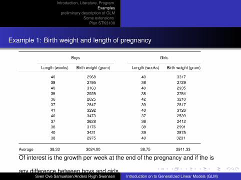
Example 1: Birth weight and length of pregnancy
Boys Girls
Length (weeks) Birth weight (gram) Length (weeks) Birth weight (gram)
40 2968 40 331738 2795 36 272940 3163 40 293535 2925 38 275436 2625 42 321037 2847 39 281741 3292 40 312640 3473 37 253937 2628 36 241238 3176 38 299140 3421 39 287538 2975 40 3231
Average 38.33 3024.00 38.75 2911.33
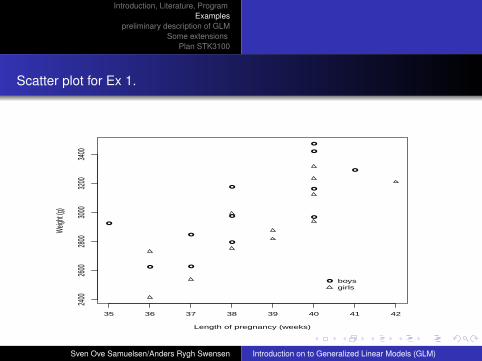
Of interest is the growth per week at the end of the pregnancy and if the is
any difference between boys and girls.Sven Ove Samuelsen/Anders Rygh Swensen Introduction on to Generalized Linear Models (GLM)
UiO
Introduction, Literature, ProgramExamples
preliminary description of GLMSome extensions
Plan STK3100
Scatter plot for Ex 1.
35 36 37 38 39 40 41 42
2400
2600
2800
3000
3200
3400
Length of pregnancy (weeks)
Weigh
t (g)
●
●
●
●
●
●
●
●
●
●
●
●
● boysgirls
Sven Ove Samuelsen/Anders Rygh Swensen Introduction on to Generalized Linear Models (GLM)
UiO
Introduction, Literature, ProgramExamples
preliminary description of GLMSome extensions
Plan STK3100
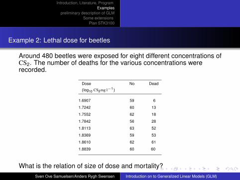
Example 2: Lethal dose for beetles
Around 480 beetles were exposed for eight different concentrations ofCS2. The number of deaths for the various concentrations wererecorded.
Dose
(log10 CS2mg l−1)
No Dead
1.6907 59 6
1.7242 60 13
1.7552 62 18
1.7842 56 28
1.8113 63 52
1.8369 59 53
1.8610 62 61
1.8839 60 60
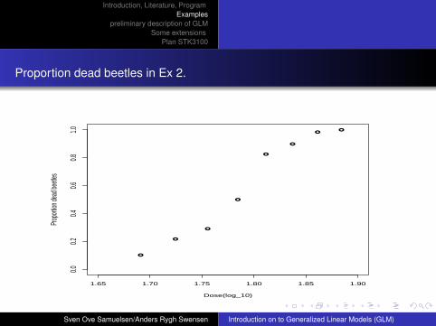
What is the relation of size of dose and mortality?Sven Ove Samuelsen/Anders Rygh Swensen Introduction on to Generalized Linear Models (GLM)
UiO
Introduction, Literature, ProgramExamples
preliminary description of GLMSome extensions
Plan STK3100
Proportion dead beetles in Ex 2.
1.65 1.70 1.75 1.80 1.85 1.90
0.00.2
0.40.6
0.81.0
Dose(log_10)
Prop
ortion
dead
beetl
es
●
●
●
●
●
●
●●
Sven Ove Samuelsen/Anders Rygh Swensen Introduction on to Generalized Linear Models (GLM)
UiO
Introduction, Literature, ProgramExamples
preliminary description of GLMSome extensions
Plan STK3100
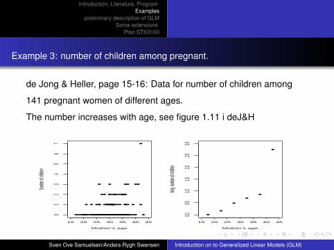
Example 3: number of children among pregnant.
de Jong & Heller, page 15-16: Data for number of children among
141 pregnant women of different ages.
The number increases with age, see figure 1.11 i deJ&H
15 20 25 30 35 40 45
01
23
45
67
Mother's age
Number
of child
ren
●
●●
●
●● ●● ●
●
●● ●●
●
●
●
●
●● ●
●
●
●●
●
●
● ●
●●
●
●
●●●
●
●
● ●● ●●
●
●● ●
●
● ●
●
●
●
●
●
●
●● ●
● ●● ●
●
●
●
●●
●
●
● ●
●
● ●
●● ●
●
●
●
●● ●● ●● ●
●
●
●
● ●
●
●● ●● ●
●
●
●●
●
●● ●●
●
●
●
●
●
●
●● ●●
●
●●● ●●●●● ●
●
●
●
●
●●●
●● ●●
● ●
15 20 25 30 35 40 45
0.00.5
1.01.5
2.02.5
3.0
Mother's age
Avrg. n
umber o
f childre
n
●
●
●
●
●
●
Sven Ove Samuelsen/Anders Rygh Swensen Introduction on to Generalized Linear Models (GLM)

UiO
Introduction, Literature, ProgramExamples
preliminary description of GLMSome extensions
Plan STK3100
Example 3b: number of third party claims
de Jong & Heller, side 17: Data over number of claims in 176
geographical regions in New South Wales in a en 12-months period.
Explanative variables, covariates:
Statistical category, 13 categories
Number of accidents in the region
Number of killed and injured
Size of population
In both examples: the response may be Poisson distributed.Sven Ove Samuelsen/Anders Rygh Swensen Introduction on to Generalized Linear Models (GLM)
UiO
Introduction, Literature, ProgramExamples
preliminary description of GLMSome extensions
Plan STK3100
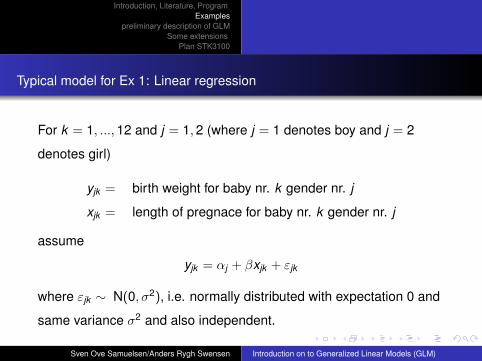
Typical model for Ex 1: Linear regression
For k = 1, ...,12 and j = 1,2 (where j = 1 denotes boy and j = 2
denotes girl)
yjk = birth weight for baby nr. k gender nr. j
xjk = length of pregnace for baby nr. k gender nr. j
assume
yjk = αj + βxjk + εjk
where εjk ∼ N(0, σ2), i.e. normally distributed with expectation 0 and
same variance σ2 and also independent.
Sven Ove Samuelsen/Anders Rygh Swensen Introduction on to Generalized Linear Models (GLM)
UiO
Introduction, Literature, ProgramExamples
preliminary description of GLMSome extensions
Plan STK3100
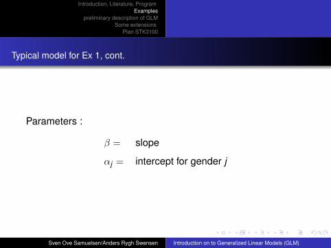
Typical model for Ex 1, cont.
Parameters :
β = slope
αj = intercept for gender j
Sven Ove Samuelsen/Anders Rygh Swensen Introduction on to Generalized Linear Models (GLM)
UiO
Introduction, Literature, ProgramExamples
preliminary description of GLMSome extensions
Plan STK3100
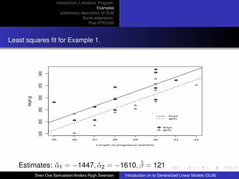
Least squares fit for Example 1.
35 36 37 38 39 40 41 42
2400
2600
2800
3000
3200
3400
Length of pregnancy (weeks)
Weigh
t (g)
●
●
●
●
●
●
●
●
●
●
●
●
boysgirls
● boysgirls
Estimates: α̂1 = −1447, α̂2 = −1610, β̂ = 121Sven Ove Samuelsen/Anders Rygh Swensen Introduction on to Generalized Linear Models (GLM)
UiO
Introduction, Literature, ProgramExamples
preliminary description of GLMSome extensions
Plan STK3100
Alternative formulation Ex. 1
Linearity: E[yjk ] = µjk = αj + βxjk
Constant variance: Var[yjk ] = σ2
Normality assumption: yjk ∼ N(µjk , σ2)
Independent responses: yjk ’s independent
Sven Ove Samuelsen/Anders Rygh Swensen Introduction on to Generalized Linear Models (GLM)
UiO
Introduction, Literature, ProgramExamples
preliminary description of GLMSome extensions
Plan STK3100
Alternative formulation Ex. 1, cont
I GLM ( and STK3100 ) three first features are modified to
Linearity after transformation via "link-function" g():
g(µjk ) = αj + βxjk
Variance may depend on the expectation of the responses.
Other distributions for the responses: Binomial, Poisson,
Gamma, ...
But independent responses are still assumed.
Sven Ove Samuelsen/Anders Rygh Swensen Introduction on to Generalized Linear Models (GLM)
UiO
Introduction, Literature, ProgramExamples
preliminary description of GLMSome extensions
Plan STK3100
EX. 2: Mortality of beetles
It is reasonable to assume yi = number dead beetles for dose xi is
binomially distributed. yi ∼ bin(ni , πi)
where πi = probability for beetle dying with dose xi and
ni = number of beetles receiving dose xi .
Linear model for πi fitted with least squares problematic because
0 ≤ πi ≤ 1 in contrast to expression α+ βxi
Var(yi) = niπi(1 − πi), i.e. non-constant (heteroskedastisc)
structure of variance
Sven Ove Samuelsen/Anders Rygh Swensen Introduction on to Generalized Linear Models (GLM)
UiO
Introduction, Literature, ProgramExamples
preliminary description of GLMSome extensions
Plan STK3100
Usual model for Ex. 2: Logistic regression
Logistic model of regression:
πi =exp(α+ βxi)
1 + exp(α+ βxi)
Then 0 ≤ πi ≤ 1
Fit the logistic model of regression with Maximum Likelihood (ML).
Takes into account binomially distributed responses (and
non-constant variance)
Efficient estimators (approximately for large data)
Sven Ove Samuelsen/Anders Rygh Swensen Introduction on to Generalized Linear Models (GLM)
UiO
Introduction, Literature, ProgramExamples
preliminary description of GLMSome extensions
Plan STK3100
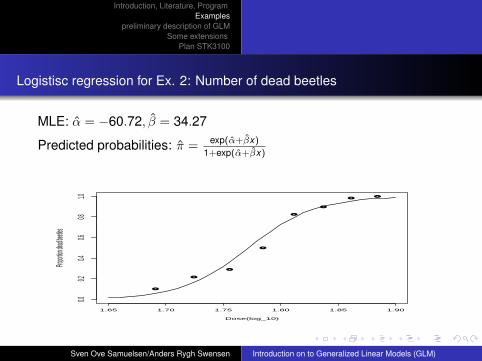
Logistisc regression for Ex. 2: Number of dead beetles
MLE: α̂ = −60.72, β̂ = 34.27
Predicted probabilities: π̂ = exp(α̂+β̂x)1+exp(α̂+β̂x)
1.65 1.70 1.75 1.80 1.85 1.90
0.00.2
0.40.6
0.81.0
Dose(log_10)
Propor
tion dea
d beetle
s
●
●
●
●
●
●
●●
Sven Ove Samuelsen/Anders Rygh Swensen Introduction on to Generalized Linear Models (GLM)
UiO
Introduction, Literature, ProgramExamples
preliminary description of GLMSome extensions
Plan STK3100
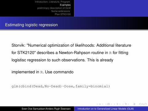
Estimating logistic regression
Storvik: "Numerical optimization of likelihoods: Additional literature
for STK2120" describes a Newton-Rahpson routine in R for fitting
logistisc regression to such observations. This is already
implemented in R. Use commando
glm(cbind(Dead,No-Dead)~Dose,family=binomial)
Sven Ove Samuelsen/Anders Rygh Swensen Introduction on to Generalized Linear Models (GLM)
UiO
Introduction, Literature, ProgramExamples
preliminary description of GLMSome extensions
Plan STK3100
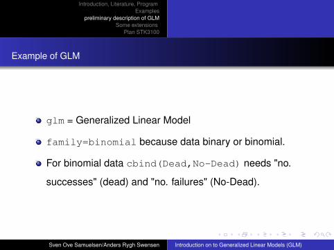
Example of GLM
glm = Generalized Linear Model
family=binomial because data binary or binomial.
For binomial data cbind(Dead,No-Dead) needs "no.
successes" (dead) and "no. failures" (No-Dead).
Sven Ove Samuelsen/Anders Rygh Swensen Introduction on to Generalized Linear Models (GLM)
UiO
Introduction, Literature, ProgramExamples
preliminary description of GLMSome extensions
Plan STK3100
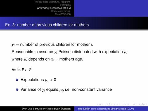
Ex. 3: number of previous children for mothers
yi = number of previous children for mother i .
Reasonable to assume yi Poisson distributed with expectation µi
where µi depends on xi = mothers age.
As in Ex. 2:
Expectations µi > 0
Variance of yi equals µi , i.e. non-constant variance
Sven Ove Samuelsen/Anders Rygh Swensen Introduction on to Generalized Linear Models (GLM)
UiO
Introduction, Literature, ProgramExamples
preliminary description of GLMSome extensions
Plan STK3100
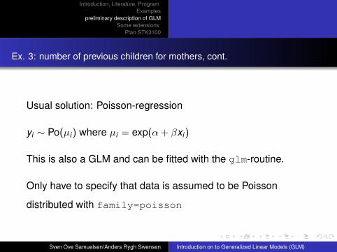
Ex. 3: number of previous children for mothers, cont.
Usual solution: Poisson-regression
yi ∼ Po(µi) where µi = exp(α+ βxi)
This is also a GLM and can be fitted with the glm-routine.
Only have to specify that data is assumed to be Poisson
distributed with family=poisson
Sven Ove Samuelsen/Anders Rygh Swensen Introduction on to Generalized Linear Models (GLM)
UiO
Introduction, Literature, ProgramExamples
preliminary description of GLMSome extensions
Plan STK3100
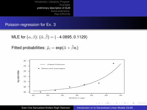
Poisson-regression for Ex. 3
MLE for (α, β): (α̂, β̂) = (−4.0895,0.1129)
Fitted probabilities: µ̂i = exp(α̂+ β̂xi)
15 20 25 30 35 40 45
0.00.5
1.01.5
2.02.5
3.0
Mother's age
Avrg. n
umber o
f childre
n
●
●
●
●
●
●
Fitted Poisson
● Observed averages
Sven Ove Samuelsen/Anders Rygh Swensen Introduction on to Generalized Linear Models (GLM)
UiO
Introduction, Literature, ProgramExamples
preliminary description of GLMSome extensions
Plan STK3100
Definition of GLM
Independent responses y1, y2, . . . , yn
Vectors of covariates x1,x2, . . . ,xn
where xi = (xi1, xi2, . . . , xip) er p-dimensional
A GLM = Generalized Linear Model is defined by the following three
components:
Sven Ove Samuelsen/Anders Rygh Swensen Introduction on to Generalized Linear Models (GLM)
UiO
Introduction, Literature, ProgramExamples
preliminary description of GLMSome extensions
Plan STK3100
Definition of GLM, cont.
y1, y2, . . . , yn has a distribution belonging to an exponential
family
(Exponential families will be defined later, suffices to know
that normal-, binomial-, Poisson-, gamma-distributions
belong to the exponential family)
Linear components (predictors) ηi = β0 +β1xi1 + · · ·+βpxip
Link function g(): The expectation µi = E[yi ] is related to
the linear component by g(µi) = ηi
Sven Ove Samuelsen/Anders Rygh Swensen Introduction on to Generalized Linear Models (GLM)
UiO
Introduction, Literature, ProgramExamples
preliminary description of GLMSome extensions
Plan STK3100
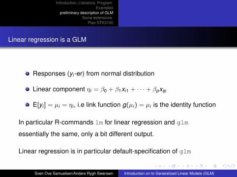
Linear regression is a GLM
Responses (yi -er) from normal distribution
Linear component ηi = β0 + β1xi1 + · · ·+ βpxip
E[yi ] = µi = ηi , i.e link function g(µi) = µi is the identity function
In particular R-commands lm for linear regression and glm
essentially the same, only a bit different output.
Linear regression is in particular default-specification of glm
Sven Ove Samuelsen/Anders Rygh Swensen Introduction on to Generalized Linear Models (GLM)
UiO
Introduction, Literature, ProgramExamples
preliminary description of GLMSome extensions
Plan STK3100
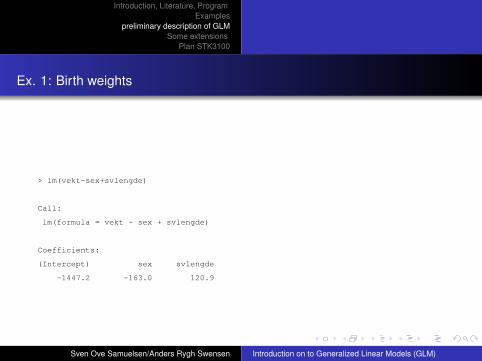
Ex. 1: Birth weights
> lm(vekt~sex+svlengde)
Call:
lm(formula = vekt ~ sex + svlengde)
Coefficients:
(Intercept) sex svlengde
-1447.2 -163.0 120.9
Sven Ove Samuelsen/Anders Rygh Swensen Introduction on to Generalized Linear Models (GLM)
UiO
Introduction, Literature, ProgramExamples
preliminary description of GLMSome extensions
Plan STK3100
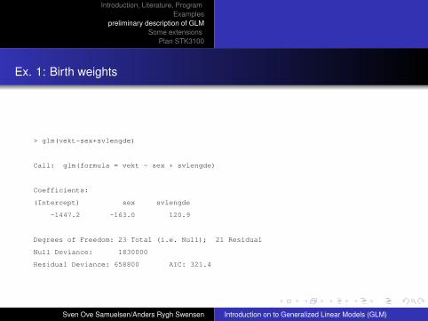
Ex. 1: Birth weights
> glm(vekt~sex+svlengde)
Call: glm(formula = vekt ~ sex + svlengde)
Coefficients:
(Intercept) sex svlengde
-1447.2 -163.0 120.9
Degrees of Freedom: 23 Total (i.e. Null); 21 Residual
Null Deviance: 1830000
Residual Deviance: 658800 AIC: 321.4
Sven Ove Samuelsen/Anders Rygh Swensen Introduction on to Generalized Linear Models (GLM)
UiO
Introduction, Literature, ProgramExamples
preliminary description of GLMSome extensions
Plan STK3100
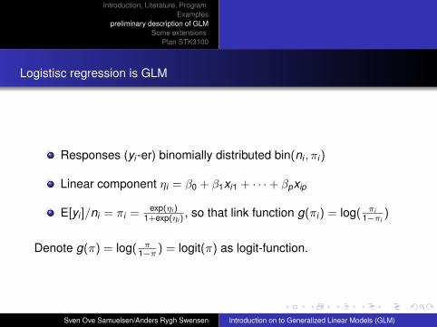
Logistisc regression is GLM
Responses (yi -er) binomially distributed bin(ni , πi)
Linear component ηi = β0 + β1xi1 + · · ·+ βpxip
E[yi ]/ni = πi =exp(ηi )
1+exp(ηi ), so that link function g(πi) = log( πi
1−πi)
Denote g(π) = log( π1−π ) = logit(π) as logit-function.
Sven Ove Samuelsen/Anders Rygh Swensen Introduction on to Generalized Linear Models (GLM)
UiO
Introduction, Literature, ProgramExamples
preliminary description of GLMSome extensions
Plan STK3100
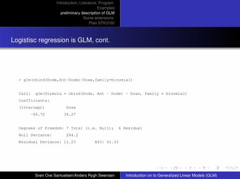
Logistisc regression is GLM, cont.
> glm(cbind(Dode,Ant-Dode)~Dose,family=binomial)
Call: glm(formula = cbind(Dode, Ant - Dode) ~ Dose, family = binomial)
Coefficients:
(Intercept) Dose
-60.72 34.27
Degrees of Freedom: 7 Total (i.e. Null); 6 Residual
Null Deviance: 284.2
Residual Deviance: 11.23 AIC: 41.43
Sven Ove Samuelsen/Anders Rygh Swensen Introduction on to Generalized Linear Models (GLM)
UiO
Introduction, Literature, ProgramExamples
preliminary description of GLMSome extensions
Plan STK3100
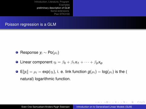
Poisson regression is a GLM
Response yi ∼ Po(µi)
Linear component ηi = β0 + β1xi1 + · · ·+ βpxip
E[yi ] = µi = exp(ηi), i. e. link function g(µi) = log(µi) is the (
natural) logarithmic function.
Sven Ove Samuelsen/Anders Rygh Swensen Introduction on to Generalized Linear Models (GLM)
UiO
Introduction, Literature, ProgramExamples
preliminary description of GLMSome extensions
Plan STK3100
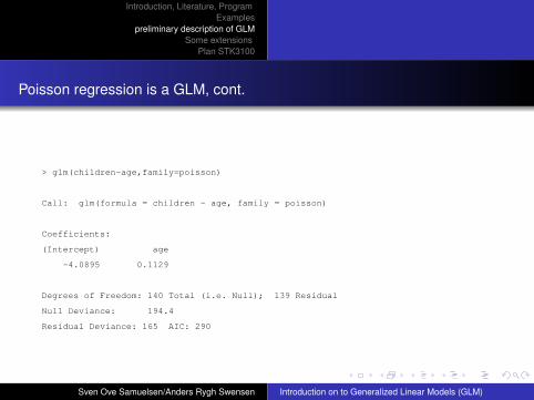
Poisson regression is a GLM, cont.
> glm(children~age,family=poisson)
Call: glm(formula = children ~ age, family = poisson)
Coefficients:
(Intercept) age
-4.0895 0.1129
Degrees of Freedom: 140 Total (i.e. Null); 139 Residual
Null Deviance: 194.4
Residual Deviance: 165 AIC: 290
Sven Ove Samuelsen/Anders Rygh Swensen Introduction on to Generalized Linear Models (GLM)
UiO
Introduction, Literature, ProgramExamples
preliminary description of GLMSome extensions
Plan STK3100
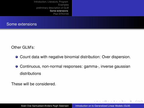
Some extensions
Other GLM’s:
Count data with negative binomial distribution: Over dispersion.
Continuous, non-normal responses: gamma-, inverse gaussian
distributions
These will be considered.
Sven Ove Samuelsen/Anders Rygh Swensen Introduction on to Generalized Linear Models (GLM)
UiO
Introduction, Literature, ProgramExamples
preliminary description of GLMSome extensions
Plan STK3100
Some other extensions
Extensions of GLM:
Multinomial responses (ordinal and nominal)
Life time data
Analysis of dependent data,GLMM
Generalized additive models (GAM)
We will consider multinomial responses and GLMM.
Sven Ove Samuelsen/Anders Rygh Swensen Introduction on to Generalized Linear Models (GLM)
UiO
Introduction, Literature, ProgramExamples
preliminary description of GLMSome extensions
Plan STK3100
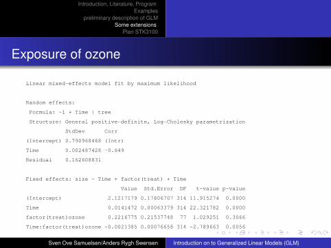
Example 4: Growth of trees and ozone exposure
Growth for two groups of trees is recorded at five different
points of time. Of the trees 54 are located in an environment
with heavy traffic and 25 trees are a control group. In total there
are 395 measurements yi,j , i = 1, · · · ,79, j = 1, · · · ,5.
Sven Ove Samuelsen/Anders Rygh Swensen Introduction on to Generalized Linear Models (GLM)
UiO
Introduction, Literature, ProgramExamples
preliminary description of GLMSome extensions
Plan STK3100
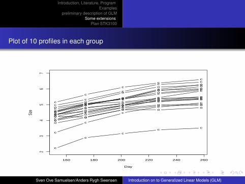
Plot of 10 profiles in each group
160 180 200 220 240 260
23
45
67
Day
Size
o
o
o
oo
c
cc
c c
o o
oo oc
c
c
cc
o
o
oo o
c
cc
cc
o
o
oo o
c
c
c
cc
o
o
o
o
o
c
c
c
c
c
o
o
o
oo
c
c
c
c c
oo
o
o oc
c
c
cc
o
o
o
o o
c
c
c
cc
o
o
o
oo
c
c
c
c
c
o
o
o oo
c
c
cc
c
Sven Ove Samuelsen/Anders Rygh Swensen Introduction on to Generalized Linear Models (GLM)
UiO
Introduction, Literature, ProgramExamples
preliminary description of GLMSome extensions
Plan STK3100
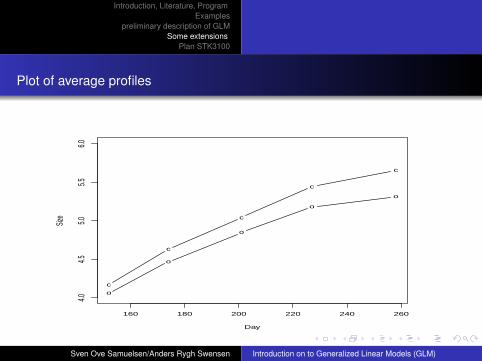
Plot of average profiles
160 180 200 220 240 260
4.04.5
5.05.5
6.0
Day
Size
o
o
o
o
o
c
c
c
c
c
Sven Ove Samuelsen/Anders Rygh Swensen Introduction on to Generalized Linear Models (GLM)
UiO
Introduction, Literature, ProgramExamples
preliminary description of GLMSome extensions
Plan STK3100
Exposure of ozone
Linear mixed-effects model fit by maximum likelihood
Random effects:
Formula: ~1 + Time | tree
Structure: General positive-definite, Log-Cholesky parametrization
StdDev Corr
(Intercept) 0.790968468 (Intr)
Time 0.002487428 -0.649
Residual 0.162608831
Fixed effects: size ~ Time + factor(treat) * Time
Value Std.Error DF t-value p-value
(Intercept) 2.1217179 0.17806707 314 11.915274 0.0000
Time 0.0141472 0.00063379 314 22.321782 0.0000
factor(treat)ozone 0.2216775 0.21537748 77 1.029251 0.3066
Time:factor(treat)ozone -0.0021385 0.00076658 314 -2.789663 0.0056
Sven Ove Samuelsen/Anders Rygh Swensen Introduction on to Generalized Linear Models (GLM)
UiO
Introduction, Literature, ProgramExamples
preliminary description of GLMSome extensions
Plan STK3100
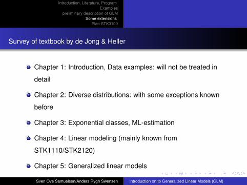
Survey of textbook by de Jong & Heller
Chapter 1: Introduction, Data examples: will not be treated in
detail
Chapter 2: Diverse distributions: with some exceptions known
before
Chapter 3: Exponential classes, ML-estimation
Chapter 4: Linear modeling (mainly known from
STK1110/STK2120)
Chapter 5: Generalized linear models
Sven Ove Samuelsen/Anders Rygh Swensen Introduction on to Generalized Linear Models (GLM)
UiO
Introduction, Literature, ProgramExamples
preliminary description of GLMSome extensions
Plan STK3100
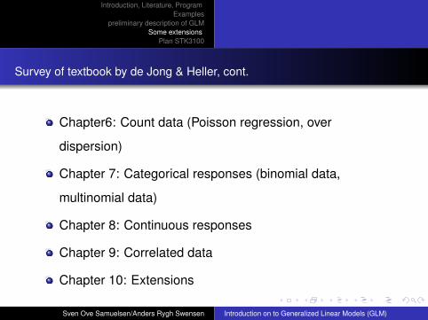
Survey of textbook by de Jong & Heller, cont.
Chapter6: Count data (Poisson regression, over
dispersion)
Chapter 7: Categorical responses (binomial data,
multinomial data)
Chapter 8: Continuous responses
Chapter 9: Correlated data
Chapter 10: Extensions
Sven Ove Samuelsen/Anders Rygh Swensen Introduction on to Generalized Linear Models (GLM)
UiO
Introduction, Literature, ProgramExamples
preliminary description of GLMSome extensions
Plan STK3100
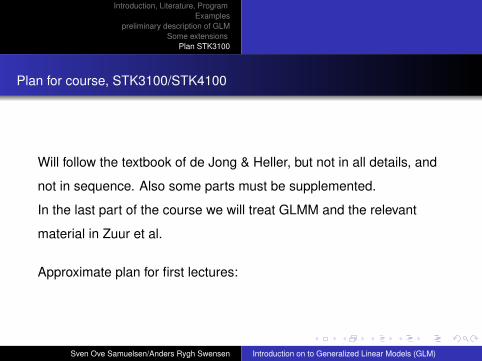
Plan for course, STK3100/STK4100
Will follow the textbook of de Jong & Heller, but not in all details, and
not in sequence. Also some parts must be supplemented.
In the last part of the course we will treat GLMM and the relevant
material in Zuur et al.
Approximate plan for first lectures:
Sven Ove Samuelsen/Anders Rygh Swensen Introduction on to Generalized Linear Models (GLM)
UiO
Introduction, Literature, ProgramExamples
preliminary description of GLMSome extensions
Plan STK3100
Plan for course, STK3100/STK4100, cont.
Introduction, today!
Chapter 4. Linear models, mainly repetition of
STK1110/STK2120, Thursday August 20th and Tuesday
August 25th
Chapter 3: Exponential classes, September 1st.
Chapter 5: GLM and ML-theory September 8th.
Chapter 7: Binomial and binary data
Chapter 6: Count data
Sven Ove Samuelsen/Anders Rygh Swensen Introduction on to Generalized Linear Models (GLM)
UiO
Introduction, Literature, ProgramExamples
preliminary description of GLMSome extensions
Plan STK3100
Plan for course, STK3100/STK4100, cont.
Chapter 7: Multinomial data
Chapter 8: A little of continuous responses
Extensions: Correlated data and GAM, material from Zuur et al.
chapters 6, 7 and 13.
Sven Ove Samuelsen/Anders Rygh Swensen Introduction on to Generalized Linear Models (GLM)