glm — Generalized linear models · or Newton–Raphson ... (binomial) Logit model of y events occurring in 15 trials as a function of x glm y x, ... glm— Generalized linear models

Title stata.com

glm — Generalized linear models

Description Quick start Menu SyntaxOptions Remarks and examples Stored results Methods and formulasAcknowledgments References Also see

Descriptionglm fits generalized linear models. It can fit models by using either IRLS (maximum quasilikelihood)

or Newton–Raphson (maximum likelihood) optimization, which is the default.

See [U] 26 Overview of Stata estimation commands for a description of all of Stata’s estimationcommands, several of which fit models that can also be fit using glm.

Quick startModel of y as a function of x when y is a proportion

glm y x, family(binomial)

Logit model of y events occurring in 15 trials as a function of xglm y x, family(binomial 15) link(logit)

Probit model of y events as a function of x using grouped data with group sizes n

glm y x, family(binomial n) link(probit)

Model of discrete y with user-defined family myfamily and link mylink

glm y x, family(myfamily) link(mylink)

Bootstrap standard errors in a model of y as a function of x with a gamma family and log linkglm y x, family(gamma) link(log) vce(bootstrap)

MenuStatistics > Generalized linear models > Generalized linear models (GLM)

1

http://stata.com

http://www.stata.com/manuals/u26.pdf#u26OverviewofStataestimationcommands

2 glm — Generalized linear models

Syntaxglm depvar

[indepvars

] [if] [

in] [

weight] [

, options]

options Description

Model

family(familyname) distribution of depvar; default is family(gaussian)

link(linkname) link function; default is canonical link for family() specified

Model 2

noconstant suppress constant termexposure(varname) include ln(varname) in model with coefficient constrained to 1offset(varname) include varname in model with coefficient constrained to 1constraints(constraints) apply specified linear constraintscollinear keep collinear variablesasis retain perfect predictor variablesmu(varname) use varname as the initial estimate for the mean of depvarinit(varname) synonym for mu(varname)

SE/Robust

vce(vcetype) vcetype may be oim, robust, cluster clustvar, eim, opg,bootstrap, jackknife, hac kernel, jackknife1, or unbiased

vfactor(#) multiply variance matrix by scalar #disp(#) quasilikelihood multiplierscale(x2 | dev | #) set the scale parameter

Reporting

level(#) set confidence level; default is level(95)

eform report exponentiated coefficientsnocnsreport do not display constraintsdisplay options control columns and column formats, row spacing, line width,

display of omitted variables and base and empty cells, andfactor-variable labeling

Maximization

ml use maximum likelihood optimization; the defaultirls use iterated, reweighted least-squares optimization of the deviancemaximize options control the maximization process; seldom usedfisher(#) use the Fisher scoring Hessian or expected information matrix (EIM)search search for good starting values

noheader suppress header table from above coefficient tablenotable suppress coefficient tablenodisplay suppress the output; iteration log is still displayedcoeflegend display legend instead of statistics

http://www.stata.com/manuals/u11.pdf#u11.4varnameandvarlists


http://www.stata.com/manuals/u11.pdf#u11.1.3ifexp

http://www.stata.com/manuals/u11.pdf#u11.1.4inrange




http://www.stata.com/manuals/restimationoptions.pdf#restimationoptionsOptionsconstraintsdescrip




glm — Generalized linear models 3

familyname Description

gaussian Gaussian (normal)igaussian inverse Gaussianbinomial

[varnameN | #N

]Bernoulli/binomial

poisson Poissonnbinomial

[#k | ml

]negative binomial

gamma gamma

linkname Description

identity identitylog loglogit logitprobit probitcloglog clog-logpower # poweropower # odds powernbinomial negative binomialloglog log-loglogc log-complement

indepvars may contain factor variables; see [U] 11.4.3 Factor variables.depvar and indepvars may contain time-series operators; see [U] 11.4.4 Time-series varlists.bayes, bootstrap, by, fmm, fp, jackknife, mfp, mi estimate, nestreg, rolling, statsby, stepwise, and svy

are allowed; see [U] 11.1.10 Prefix commands. For more details, see [BAYES] bayes: glm and [FMM] fmm: glm.vce(bootstrap), vce(jackknife), and vce(jackknife1) are not allowed with the mi estimate prefix; see

[MI] mi estimate.Weights are not allowed with the bootstrap prefix; see [R] bootstrap.aweights are not allowed with the jackknife prefix; see [R] jackknife.vce(), vfactor(), disp(), scale(), irls, fisher(), noheader, notable, nodisplay, and weights are not

allowed with the svy prefix; see [SVY] svy.fweights, aweights, iweights, and pweights are allowed; see [U] 11.1.6 weight.noheader, notable, nodisplay, and coeflegend do not appear in the dialog box.See [U] 20 Estimation and postestimation commands for more capabilities of estimation commands.

Options

� � �Model �

family( familyname) specifies the distribution of depvar; family(gaussian) is the default.

link(linkname) specifies the link function; the default is the canonical link for the family()specified (except for family(nbinomial)).

� � �Model 2 �

noconstant, exposure(varname), offset(varname), constraints(constraints), collinear;see [R] estimation options. constraints(constraints) and collinear are not allowed withirls.


http://www.stata.com/manuals/u11.pdf#u11.4.3Factorvariables

http://www.stata.com/manuals/u11.pdf#u11.4.4Time-seriesvarlists

http://www.stata.com/manuals/u11.pdf#u11.1.10Prefixcommands

http://www.stata.com/manuals/bayesbayesglm.pdf#bayesbayesglm

http://www.stata.com/manuals/fmmfmmglm.pdf#fmmfmmglm

http://www.stata.com/manuals/mimiestimate.pdf#mimiestimate

http://www.stata.com/manuals/rbootstrap.pdf#rbootstrap

http://www.stata.com/manuals/rjackknife.pdf#rjackknife

http://www.stata.com/manuals/svysvy.pdf#svysvy

http://www.stata.com/manuals/u11.pdf#u11.1.6weight

http://www.stata.com/manuals/u20.pdf#u20Estimationandpostestimationcommands



http://www.stata.com/manuals/restimationoptions.pdf#restimationoptions


asis forces retention of perfect predictor variables and their associated, perfectly predicted observationsand may produce instabilities in maximization; see [R] probit. This option is only allowed withoption family(binomial) with a denominator of 1.

mu(varname) specifies varname as the initial estimate for the mean of depvar. This option can beuseful with models that experience convergence difficulties, such as family(binomial) modelswith power or odds-power links. init(varname) is a synonym.

� � �SE/Robust �

vce(vcetype) specifies the type of standard error reported, which includes types that are derived fromasymptotic theory (oim, opg), that are robust to some kinds of misspecification (robust), thatallow for intragroup correlation (cluster clustvar), and that use bootstrap or jackknife methods(bootstrap, jackknife); see [R] vce option.

In addition to the standard vcetypes, glm allows the following alternatives:

vce(eim) specifies that the EIM estimate of variance be used.

vce(jackknife1) specifies that the one-step jackknife estimate of variance be used.

vce(hac kernel[#]) specifies that a heteroskedasticity- and autocorrelation-consistent (HAC)

variance estimate be used. HAC refers to the general form for combining weighted matricesto form the variance estimate. There are three kernels built into glm. kernel is a community-contributed program or one of

nwest | gallant | anderson# specifies the number of lags. If # is not specified, N − 2 is assumed. If you wish to specifyvce(hac . . . ), you must tsset your data before calling glm.

vce(unbiased) specifies that the unbiased sandwich estimate of variance be used.

vfactor(#) specifies a scalar by which to multiply the resulting variance matrix. This option allowsyou to match output with other packages, which may apply degrees of freedom or other small-samplecorrections to estimates of variance.

disp(#) multiplies the variance of depvar by # and divides the deviance by #. The resultingdistributions are members of the quasilikelihood family.

scale(x2 | dev | #) overrides the default scale parameter. This option is allowed only with Hessian(information matrix) variance estimates.

By default, scale(1) is assumed for the discrete distributions (binomial, Poisson, and negativebinomial), and scale(x2) is assumed for the continuous distributions (Gaussian, gamma, andinverse Gaussian).

scale(x2) specifies that the scale parameter be set to the Pearson chi-squared (or generalized chi-squared) statistic divided by the residual degrees of freedom, which is recommended by McCullaghand Nelder (1989) as a good general choice for continuous distributions.

scale(dev) sets the scale parameter to the deviance divided by the residual degrees of freedom.This option provides an alternative to scale(x2) for continuous distributions and overdispersedor underdispersed discrete distributions.

scale(#) sets the scale parameter to #. For example, using scale(1) in family(gamma)models results in exponential-errors regression. Additional use of link(log) rather than thedefault link(power -1) for family(gamma) essentially reproduces Stata’s streg, dist(exp)nohr command (see [ST] streg) if all the observations are uncensored.

http://www.stata.com/manuals/rprobit.pdf#rprobit



http://www.stata.com/manuals/rvce_option.pdf#rvce_option


http://www.stata.com/manuals/ststreg.pdf#ststreg


� � �Reporting �

level(#); see [R] estimation options.

eform displays the exponentiated coefficients and corresponding standard errors and confidenceintervals. For family(binomial) link(logit) (that is, logistic regression), exponentiationresults are odds ratios; for family(nbinomial) link(log) (that is, negative binomial regression)and for family(poisson) link(log) (that is, Poisson regression), exponentiated coefficientsare incidence-rate ratios.

nocnsreport; see [R] estimation options.

display options: noci, nopvalues, noomitted, vsquish, noemptycells, baselevels,allbaselevels, nofvlabel, fvwrap(#), fvwrapon(style), cformat(% fmt), pformat(% fmt),sformat(% fmt), and nolstretch; see [R] estimation options.

� � �Maximization �

ml requests that optimization be carried out using Stata’s ml commands and is the default.

irls requests iterated, reweighted least-squares (IRLS) optimization of the deviance instead of Newton–Raphson optimization of the log likelihood. If the irls option is not specified, the optimizationis carried out using Stata’s ml commands, in which case all options of ml maximize are alsoavailable.

maximize options: difficult, technique(algorithm spec), iterate(#),[no]log, trace,

gradient, showstep, hessian, showtolerance, tolerance(#), ltolerance(#),nrtolerance(#), nonrtolerance, and from(init specs); see [R] maximize. These options areseldom used.

Setting the optimization type to technique(bhhh) resets the default vcetype to vce(opg).

fisher(#) specifies the number of Newton–Raphson steps that should use the Fisher scoring Hessianor EIM before switching to the observed information matrix (OIM). This option is useful only forNewton–Raphson optimization (and not when using irls).

search specifies that the command search for good starting values. This option is useful only forNewton–Raphson optimization (and not when using irls).

The following options are available with glm but are not shown in the dialog box:

noheader suppresses the header information from the output. The coefficient table is still displayed.

notable suppresses the table of coefficients from the output. The header information is still displayed.

nodisplay suppresses the output. The iteration log is still displayed.

coeflegend; see [R] estimation options.

Remarks and examples stata.com

Remarks are presented under the following headings:

General useVariance estimatorsUser-defined functions



http://www.stata.com/manuals/d.pdf#dformat


http://www.stata.com/manuals/rmaximize.pdf#rmaximizeSyntaxalgorithm_spec

http://www.stata.com/manuals/rmaximize.pdf#rmaximize


http://stata.com


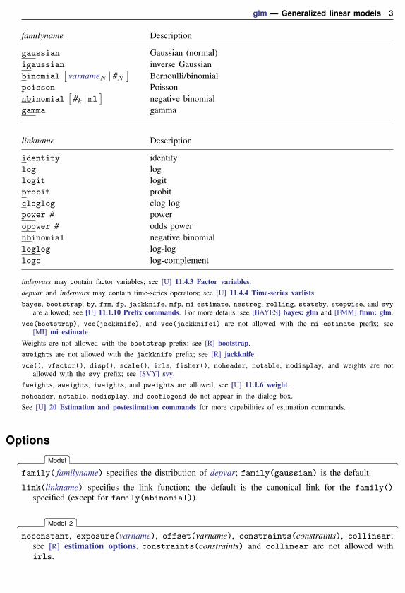
General use

glm fits generalized linear models of y with covariates x:

g{E(y)

}= xβ, y ∼ F

g( ) is called the link function, and F is the distributional family. Substituting various definitionsfor g( ) and F results in a surprising array of models. For instance, if y is distributed as Gaussian(normal) and g( ) is the identity function, we have

E(y) = xβ, y ∼ Normal

or linear regression. If g( ) is the logit function and y is distributed as Bernoulli, we have

logit{E(y)

}= xβ, y ∼ Bernoulli

or logistic regression. If g( ) is the natural log function and y is distributed as Poisson, we have

ln{E(y)

}= xβ, y ∼ Poisson

or Poisson regression, also known as the log-linear model. Other combinations are possible.

Although glm can be used to perform linear regression (and, in fact, does so by default), thisregression should be viewed as an instructional feature; regress produces such estimates morequickly, and many postestimation commands are available to explore the adequacy of the fit; see[R] regress and [R] regress postestimation.

In any case, you specify the link function by using the link() option and specify the distributionalfamily by using family(). The available link functions are

Link function glm option

identity link(identity)

log link(log)

logit link(logit)

probit link(probit)

complementary log-log link(cloglog)

odds power link(opower #)

power link(power #)

negative binomial link(nbinomial)

log-log link(loglog)

log-complement link(logc)

Define µ = E(y) and η = g(µ), meaning that g(·) maps E(y) to η = xβ + offset.

http://www.stata.com/manuals/rregress.pdf#rregress

http://www.stata.com/manuals/rregresspostestimation.pdf#rregresspostestimation


Link functions are defined as follows:

identity is defined as η = g(µ) = µ.

log is defined as η = ln(µ).

logit is defined as η = ln{µ/(1− µ)

}, the natural log of the odds.

probit is defined as η = Φ−1(µ), where Φ−1( ) is the inverse Gaussian cumulative.

cloglog is defined as η = ln{− ln(1− µ)

}.

opower is defined as η =[{µ/(1 − µ)

}n − 1]/n, the power of the odds. The function is

generalized so that link(opower 0) is equivalent to link(logit), the natural log of the odds.

power is defined as η = µn. Specifying link(power 1) is equivalent to specifyinglink(identity). The power function is generalized so that µ0 ≡ ln(µ). Thus link(power0) is equivalent to link(log). Negative powers are, of course, allowed.

nbinomial is defined as η = ln{µ/(µ+ k)

}, where k = 1 if family(nbinomial) is specified,

k = #k if family(nbinomial #k) is specified, and k is estimated via maximum likelihood iffamily(nbinomial ml) is specified.

loglog is defined as η = −ln{−ln(µ)}.logc is defined as η = ln(1− µ).

The available distributional families are

Family glm option

Gaussian (normal) family(gaussian)

inverse Gaussian family(igaussian)

Bernoulli/binomial family(binomial)

Poisson family(poisson)

negative binomial family(nbinomial)

gamma family(gamma)

family(normal) is a synonym for family(gaussian).

The binomial distribution can be specified as 1) family(binomial), 2) family(binomial #N),or 3) family(binomial varnameN). In case 2, #N is the value of the binomial denominator N , thenumber of trials. Specifying family(binomial 1) is the same as specifying family(binomial).In case 3, varnameN is the variable containing the binomial denominator, allowing the number oftrials to vary across observations.

The negative binomial distribution can be specified as 1) family(nbinomial), 2) fam-ily(nbinomial #k), or 3) family(nbinomial ml). Omitting #k is equivalent to specifyingfamily(nbinomial 1). In case 3, the value of #k is estimated via maximum likelihood. The value#k enters the variance and deviance functions. Typical values range between 0.01 and 2; see thetechnical note below.

You do not have to specify both family() and link(); the default link() is the canonical linkfor the specified family() (except for nbinomial):


Family Default link

family(gaussian) link(identity)

family(igaussian) link(power -2)

family(binomial) link(logit)

family(poisson) link(log)

family(nbinomial) link(log)

family(gamma) link(power -1)

If you specify both family() and link(), not all combinations make sense. You may choose fromthe following combinations:

identity log logit probit cloglog power opower nbinomial loglog logc

Gaussian x x xinverse Gaussian x x xbinomial x x x x x x x x xPoisson x x xnegative binomial x x x xgamma x x x

Technical note

Some family() and link() combinations result in models already fit by Stata. These are

family() link() Options Equivalent Stata command

gaussian identity nothing | irls | irls vce(oim) regress

gaussian identity t(var) vce(hac nwest #) newey, t(var) lag(#) (see note 1)vfactor(#v)

binomial cloglog nothing | irls vce(oim) cloglog (see note 2)

binomial probit nothing | irls vce(oim) probit (see note 2)

binomial logit nothing | irls | irls vce(oim) logit or logistic (see note 3)

poisson log nothing | irls | irls vce(oim) poisson (see note 3)

nbinomial log nothing | irls vce(oim) nbreg (see note 4)gamma log scale(1) streg, dist(exp) nohr (see note 5)

Notes:

1. The variance factor #v should be set to n/(n − k), where n is the number of observations andk the number of regressors. If the number of regressors is not specified, the estimated standarderrors will, as a result, differ by this factor.

2. Because the link is not the canonical link for the binomial family, you must specify the vce(oim)option if using irls to get equivalent standard errors. If irls is used without vce(oim),the regression coefficients will be the same but the standard errors will be only asymptoticallyequivalent. If no options are specified (nothing), glm will optimize using Newton–Raphson, makingit equivalent to the other Stata command.

See [R] cloglog and [R] probit for more details about these commands.

3. Because the canonical link is being used, the standard errors will be equivalent whether the EIMor the OIM estimator of variance is used.

http://www.stata.com/manuals/rcloglog.pdf#rcloglog

http://www.stata.com/manuals/rprobit.pdf#rprobit


4. Family negative binomial, log-link models—also known as negative binomial regressionmodels—are used for data with an overdispersed Poisson distribution. Although glm can beused to fit such models, using Stata’s maximum likelihood nbreg command is probably better. Inthe GLM approach, you specify family(nbinomial #k) and then search for a #k that results inthe deviance-based dispersion being 1. You can also specify family(nbinomial ml) to estimate#k via maximum likelihood, which will report the same value returned from nbreg. However,nbreg also reports a confidence interval for it; see [R] nbreg and Rogers (1993). Of course, glmallows links other than log, and for those links, including the canonical nbinomial link, you willneed to use glm.

5. glm can be used to estimate parameters from exponential regressions, but this method requiresspecifying scale(1). However, censoring is not available. Censored exponential regression maybe modeled using glm with family(poisson). The log of the original response is entered intoa Poisson model as an offset, whereas the new response is the censor variable. The result of suchmodeling is identical to the log relative hazard parameterization of streg, dist(exp) nohr. See[ST] streg for details about the streg command.

In general, where there is overlap between a capability of glm and that of some other Statacommand, we recommend using the other Stata command. Our recommendation is not because ofsome inferiority of the GLM approach. Rather, those other commands, by being specialized, provideoptions and ancillary commands that are missing in the broader glm framework. Nevertheless, glmdoes produce the same answers where it should.

Special note. When equivalence is expected, for some datasets, you may still see very slight differencesin the results, most often only in the later digits of the standard errors. When you compare glmoutput to an equivalent Stata command, these tiny discrepancies arise for many reasons:

a. glm uses a general methodology for starting values, whereas the equivalent Stata command maybe more specialized in its treatment of starting values.

b. When using a canonical link, glm, irls should be equivalent to the maximum likelihood methodof the equivalent Stata command, yet the convergence criterion is different (one is for deviance,the other for log likelihood). These discrepancies are easily resolved by adjusting one convergencecriterion to correspond to the other.

c. When both glm and the equivalent Stata command use Newton–Raphson, small differences maystill occur if the Stata command has a different default convergence criterion from that of glm.Adjusting the convergence criterion will resolve the difference. See [R] ml and [R] maximize formore details.

Example 1

In example 1 of [R] logistic, we fit a model based on data from a study of risk factors associatedwith low birthweight (Hosmer, Lemeshow, and Sturdivant 2013, 24). We can replicate the estimationby using glm:

http://www.stata.com/manuals/rnbreg.pdf#rnbreg

http://www.stata.com/manuals/ststreg.pdf#ststreg

http://www.stata.com/manuals/rml.pdf#rml

http://www.stata.com/manuals/rmaximize.pdf#rmaximize

http://www.stata.com/manuals/rlogistic.pdf#rlogisticRemarksandexamplesex1_logistic

http://www.stata.com/manuals/rlogistic.pdf#rlogistic


. use http://www.stata-press.com/data/r15/lbw(Hosmer & Lemeshow data)

. glm low age lwt i.race smoke ptl ht ui, family(binomial) link(logit)

Iteration 0: log likelihood = -101.0213Iteration 1: log likelihood = -100.72519Iteration 2: log likelihood = -100.724Iteration 3: log likelihood = -100.724

Generalized linear models No. of obs = 189Optimization : ML Residual df = 180

Scale parameter = 1Deviance = 201.4479911 (1/df) Deviance = 1.119156Pearson = 182.0233425 (1/df) Pearson = 1.011241

Variance function: V(u) = u*(1-u) [Bernoulli]Link function : g(u) = ln(u/(1-u)) [Logit]

AIC = 1.1611Log likelihood = -100.7239956 BIC = -742.0665

OIMlow Coef. Std. Err. z P>|z| [95% Conf. Interval]

age -.0271003 .0364504 -0.74 0.457 -.0985418 .0443412lwt -.0151508 .0069259 -2.19 0.029 -.0287253 -.0015763

raceblack 1.262647 .5264101 2.40 0.016 .2309024 2.294392other .8620792 .4391532 1.96 0.050 .0013548 1.722804

smoke .9233448 .4008266 2.30 0.021 .137739 1.708951ptl .5418366 .346249 1.56 0.118 -.136799 1.220472ht 1.832518 .6916292 2.65 0.008 .4769494 3.188086ui .7585135 .4593768 1.65 0.099 -.1418484 1.658875

_cons .4612239 1.20459 0.38 0.702 -1.899729 2.822176

glm, by default, presents coefficient estimates, whereas logistic presents the exponentiatedcoefficients—the odds ratios. glm’s eform option reports exponentiated coefficients, and glm, likeStata’s other estimation commands, replays results.


. glm, eform



Variance function: V(u) = u*(1-u) [Bernoulli]Link function : g(u) = ln(u/(1-u)) [Logit]


OIMlow Odds Ratio Std. Err. z P>|z| [95% Conf. Interval]

age .9732636 .0354759 -0.74 0.457 .9061578 1.045339lwt .9849634 .0068217 -2.19 0.029 .9716834 .9984249

raceblack 3.534767 1.860737 2.40 0.016 1.259736 9.918406other 2.368079 1.039949 1.96 0.050 1.001356 5.600207

smoke 2.517698 1.00916 2.30 0.021 1.147676 5.523162ptl 1.719161 .5952579 1.56 0.118 .8721455 3.388787ht 6.249602 4.322408 2.65 0.008 1.611152 24.24199ui 2.1351 .9808153 1.65 0.099 .8677528 5.2534

_cons 1.586014 1.910496 0.38 0.702 .1496092 16.8134

Note: _cons estimates baseline odds.

These results are the same as those reported in example 1 of [R] logistic.

Included in the output header are values for the Akaike (1973) information criterion (AIC) and theBayesian information criterion (BIC) (Raftery 1995). Both are measures of model fit adjusted for thenumber of parameters that can be compared across models. In both cases, a smaller value generallyindicates a better model fit. AIC is based on the log likelihood and thus is available only whenNewton–Raphson optimization is used. BIC is based on the deviance and thus is always available.

Technical noteThe values for AIC and BIC reported in the output after glm are different from those reported by

estat ic:

. estat ic

Akaike’s information criterion and Bayesian information criterion

Model Obs ll(null) ll(model) df AIC BIC

. 189 . -100.724 9 219.448 248.6237

Note: N=Obs used in calculating BIC; see [R] BIC note.

There are various definitions of these information criteria (IC) in the literature; glm and estat icuse different definitions. glm bases its computation of the BIC on deviance, whereas estat ic usesthe likelihood. Both glm and estat ic use the likelihood to compute the AIC; however, the AIC fromestat ic is equal to N , the number of observations, times the AIC from glm. Refer to Methods andformulas in this entry and [R] estat ic for the references and formulas used by glm and estat ic,respectively, to compute AIC and BIC. Inferences based on comparison of IC values reported by glm

http://www.stata.com/manuals/rlogistic.pdf#rlogisticRemarksandexamplesex1_logistic


http://www.stata.com/manuals/restatic.pdf#restatic


for different GLM models will be equivalent to those based on comparison of IC values reported byestat ic after glm.

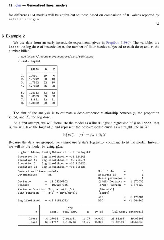
Example 2

We use data from an early insecticide experiment, given in Pregibon (1980). The variables areldose, the log dose of insecticide; n, the number of flour beetles subjected to each dose; and r, thenumber killed.

. use http://www.stata-press.com/data/r15/ldose

. list, sep(4)

ldose n r

1. 1.6907 59 62. 1.7242 60 133. 1.7552 62 184. 1.7842 56 28

5. 1.8113 63 526. 1.8369 59 537. 1.861 62 618. 1.8839 60 60

The aim of the analysis is to estimate a dose–response relationship between p, the proportionkilled, and X , the log dose.

As a first attempt, we will formulate the model as a linear logistic regression of p on ldose; thatis, we will take the logit of p and represent the dose–response curve as a straight line in X:

ln{p/(1− p)

}= β0 + β1X

Because the data are grouped, we cannot use Stata’s logistic command to fit the model. Instead,we will fit the model by using glm:

. glm r ldose, family(binomial n) link(logit)




Variance function: V(u) = u*(1-u/n) [Binomial]Link function : g(u) = ln(u/(n-u)) [Logit]


OIMr Coef. Std. Err. z P>|z| [95% Conf. Interval]

ldose 34.27034 2.912141 11.77 0.000 28.56265 39.97803_cons -60.71747 5.180713 -11.72 0.000 -70.87149 -50.56346


We specified family(binomial n), meaning that variable n contains the denominator.

An alternative model, which gives asymmetric sigmoid curves for p, involves the complementarylog-log, or clog-log, function:

ln{− ln(1− p)

}= β0 + β1X

We fit this model by using glm:

. glm r ldose, family(binomial n) link(cloglog)



Scale parameter = 1Deviance = 3.446418004 (1/df) Deviance = .574403Pearson = 3.294675153 (1/df) Pearson = .5491125

Variance function: V(u) = u*(1-u/n) [Binomial]Link function : g(u) = ln(-ln(1-u/n)) [Complementary log-log]



ldose 22.04118 1.793089 12.29 0.000 18.52679 25.55557_cons -39.57232 3.229047 -12.26 0.000 -45.90114 -33.24351

The complementary log-log model is preferred; the deviance for the logistic model, 11.23, is muchhigher than the deviance for the clog-log model, 3.45. This change also is evident by comparing loglikelihoods, or equivalently, AIC values.

This example also shows the advantage of the glm command—we can vary assumptions easily.Note the minor difference in what we typed to obtain the logistic and clog-log models:

. glm r ldose, family(binomial n) link(logit)

. glm r ldose, family(binomial n) link(cloglog)

If we were performing this work for ourselves, we would have typed the commands in a moreabbreviated form:

. glm r ldose, f(b n) l(l)

. glm r ldose, f(b n) l(cl)

Technical noteFactor variables may be used with glm. Say that, in the example above, we had ldose, the

log dose of insecticide; n, the number of flour beetles subjected to each dose; and r, the numberkilled—all as before—except that now we have results for three different kinds of beetles. Ourhypothetical data include beetle, which contains the values 1 (“Destructive flour”), 2 (“Red flour”),and 3 (“Mealworm”).


. use http://www.stata-press.com/data/r15/beetle

. list, sep(0)

beetle ldose n r

1. Destructive flour 1.6907 59 62. Destructive flour 1.7242 60 133. Destructive flour 1.7552 62 184. Destructive flour 1.7842 56 285. Destructive flour 1.8113 63 52

(output omitted )23. Mealworm 1.861 64 2324. Mealworm 1.8839 58 22

Let’s assume that, at first, we wish merely to add a shift factor for the type of beetle. We could type

. glm r i.beetle ldose, family(bin n) link(cloglog)





AIC = 6.74547Log likelihood = -76.94564525 BIC = 10.20398


beetleRed flour -.0910396 .1076132 -0.85 0.398 -.3019576 .1198783Mealworm -1.836058 .1307125 -14.05 0.000 -2.09225 -1.579867

ldose 19.41558 .9954265 19.50 0.000 17.46458 21.36658_cons -34.84602 1.79333 -19.43 0.000 -38.36089 -31.33116


We find strong evidence that the insecticide works differently on the mealworm. We now checkwhether the curve is merely shifted or also differently sloped:

. glm r beetle##c.ldose, family(bin n) link(cloglog)







beetleRed flour -.79933 4.470882 -0.18 0.858 -9.562098 7.963438Mealworm 17.78741 4.586429 3.88 0.000 8.798172 26.77664

ldose 22.04118 1.793089 12.29 0.000 18.52679 25.55557

beetle#c.ldoseRed flour .3838708 2.478477 0.15 0.877 -4.473855 5.241596Mealworm -10.726 2.526412 -4.25 0.000 -15.67768 -5.774321

_cons -39.57232 3.229047 -12.26 0.000 -45.90114 -33.24351

We find that the (complementary log-log) dose–response curve for the mealworm has roughly halfthe slope of that for the destructive flour beetle.

See [U] 25 Working with categorical data and factor variables; what is said there concerninglinear regression is applicable to any GLM model.

http://www.stata.com/manuals/u25.pdf#u25Workingwithcategoricaldataandfactorvariables


Variance estimatorsglm offers many variance options and gives different types of standard errors when used in various

combinations. We highlight some of them here, but for a full explanation, see Hardin and Hilbe (2018).

Example 3

Continuing with our flour beetle data, we rerun the most recently displayed model, this timerequesting estimation via IRLS.

. use http://www.stata-press.com/data/r15/beetle

. glm r beetle##c.ldose, f(bin n) l(cloglog) ltol(1e-13) irls

Iteration 1: deviance = 54.41414Iteration 2: deviance = 50.19424Iteration 3: deviance = 50.16973

(output omitted )Generalized linear models No. of obs = 24Optimization : MQL Fisher scoring Residual df = 18

(IRLS EIM) Scale parameter = 1Deviance = 50.16972096 (1/df) Deviance = 2.787207Pearson = 49.28422567 (1/df) Pearson = 2.738013


BIC = -7.035248

EIMr Coef. Std. Err. z P>|z| [95% Conf. Interval]


ldose 22.04118 1.799356 12.25 0.000 18.5145 25.56785


_cons -39.57232 3.240274 -12.21 0.000 -45.92314 -33.2215

Note our use of the ltol() option, which, although unrelated to our discussion on variance estimation,was used so that the regression coefficients would match those of the previous Newton–Raphson (NR)fit.

Because IRLS uses the EIM for optimization, the variance estimate is also based on EIM. If we wantoptimization via IRLS but the variance estimate based on OIM, we specify glm, irls vce(oim):


. glm r beetle##c.ldose, f(b n) l(cl) ltol(1e-15) irls vce(oim) noheader nolog



ldose 22.04118 1.793089 12.29 0.000 18.52679 25.55557


_cons -39.57232 3.229047 -12.26 0.000 -45.90114 -33.24351

This approach is identical to NR except for the convergence path. Because the clog-log link is notthe canonical link for the binomial family, EIM and OIM produce different results. Both estimators,however, are asymptotically equivalent.

Going back to NR, we can also specify vce(robust) to get the Huber/White/sandwich estimatorof variance:

. glm r beetle##c.ldose, f(b n) l(cl) vce(robust) noheader nolog

Robustr Coef. Std. Err. z P>|z| [95% Conf. Interval]


ldose 22.04118 .8998551 24.49 0.000 20.27749 23.80486


_cons -39.57232 1.621306 -24.41 0.000 -42.75003 -36.39462

The sandwich estimator gets its name from the form of the calculation—it is the multiplicationof three matrices, with the outer two matrices (the “bread”) set to the OIM variance matrix. Whenirls is used along with vce(robust), the EIM variance matrix is instead used as the bread. Usinga result from McCullagh and Nelder (1989), Newson (1999) points out that the EIM and OIM variancematrices are equivalent under the canonical link. Thus if irls is specified with the canonical link,the resulting variance is labeled “Robust”. When the noncanonical link for the family is used, whichis the case in the example below, the EIM and OIM variance matrices differ, so the resulting varianceis labeled “Semirobust”.


. glm r beetle##c.ldose, f(b n) l(cl) irls ltol(1e-15) vce(robust) noheader> nolog

Semirobustr Coef. Std. Err. z P>|z| [95% Conf. Interval]


ldose 22.04118 .9061566 24.32 0.000 20.26514 23.81721


_cons -39.57232 1.632544 -24.24 0.000 -42.77205 -36.3726

The outer product of the gradient (OPG) estimate of variance is one that avoids the calculation ofsecond derivatives. It is equivalent to the “middle” part of the sandwich estimate of variance and canbe specified by using glm, vce(opg), regardless of whether NR or IRLS optimization is used.

. glm r beetle##c.ldose, f(b n) l(cl) vce(opg) noheader nolog

OPGr Coef. Std. Err. z P>|z| [95% Conf. Interval]


ldose 22.04118 3.572983 6.17 0.000 15.03826 29.0441


_cons -39.57232 6.433101 -6.15 0.000 -52.18097 -26.96368

The OPG estimate of variance is a component of the BHHH (Berndt et al. 1974) optimizationtechnique. This method of optimization is also available with glm with the technique() option;however, the technique() option is not allowed with the irls option.

Example 4

The Newey–West (1987) estimator of variance is a sandwich estimator with the “middle” ofthe sandwich modified to take into account possible autocorrelation between the observations. Theseestimators are a generalization of those given by the Stata command newey for linear regression. See[TS] newey for more details.

For example, consider the dataset given in [TS] newey, which has time-series measurements onusr and idle. We want to perform a linear regression with Newey–West standard errors.

http://www.stata.com/manuals/tsnewey.pdf#tsnewey



. use http://www.stata-press.com/data/r15/idle2

. list usr idle time

usr idle time

1. 0 100 12. 0 100 23. 0 97 34. 1 98 45. 2 94 5

(output omitted )29. 1 98 2930. 1 98 30

Examining Methods and formulas of [TS] newey, we see that the variance estimate is multipliedby a correction factor of n/(n− k), where k is the number of regressors. glm, vce(hac . . . ) doesnot make this correction, so to get the same standard errors, we must use the vfactor() optionwithin glm to make the correction manually.

. display 30/281.0714286

. tsset timetime variable: time, 1 to 30

delta: 1 unit

. glm usr idle, vce(hac nwest 3) vfactor(1.0714286)

Iteration 0: log likelihood = -71.743396


Scale parameter = 7.493297Deviance = 209.8123165 (1/df) Deviance = 7.493297Pearson = 209.8123165 (1/df) Pearson = 7.493297

Variance function: V(u) = 1 [Gaussian]Link function : g(u) = u [Identity]

HAC kernel (lags): Newey-West (3)AIC = 4.916226

Log likelihood = -71.74339627 BIC = 114.5788

HACusr Coef. Std. Err. z P>|z| [95% Conf. Interval]

idle -.2281501 .0690928 -3.30 0.001 -.3635694 -.0927307_cons 23.13483 6.327033 3.66 0.000 10.73407 35.53558

The glm command above reproduces the results given in [TS] newey. We may now generalize thisoutput to models other than simple linear regression and to different kernel weights.

http://www.stata.com/manuals/tsnewey.pdf#tsneweyMethodsandformulas




. glm usr idle, fam(gamma) link(log) vce(hac gallant 3)



Scale parameter = .431296Deviance = 9.908506707 (1/df) Deviance = .3538752Pearson = 12.07628677 (1/df) Pearson = .431296

Variance function: V(u) = u^2 [Gamma]Link function : g(u) = ln(u) [Log]

HAC kernel (lags): Gallant (3)AIC = 4.196731

Log likelihood = -60.95096484 BIC = -85.32502

HACusr Coef. Std. Err. z P>|z| [95% Conf. Interval]

idle -.0796609 .0184647 -4.31 0.000 -.115851 -.0434708_cons 7.771011 1.510198 5.15 0.000 4.811078 10.73094

glm also offers variance estimators based on the bootstrap (resampling your data with replacement)and the jackknife (refitting the model with each observation left out in succession). Also included isthe one-step jackknife estimate, which, instead of performing full reestimation when each observationis omitted, calculates a one-step NR estimate, with the full data regression coefficients as startingvalues.

. set seed 1

. glm usr idle, fam(gamma) link(log) vce(bootstrap, reps(100) nodots)


Scale parameter = .431296Deviance = 9.908506707 (1/df) Deviance = .3538752Pearson = 12.07628677 (1/df) Pearson = .431296

Variance function: V(u) = u^2 [Gamma]Link function : g(u) = ln(u) [Log]


Observed Bootstrap Normal-basedusr Coef. Std. Err. z P>|z| [95% Conf. Interval]

idle -.0796609 .016657 -4.78 0.000 -.1123081 -.0470137_cons 7.771011 1.378037 5.64 0.000 5.070108 10.47192

See Hardin and Hilbe (2018) for a full discussion of the variance options that go with glm and,in particular, of how the different variance estimators are modified when vce(cluster clustvar) isspecified. Finally, not all variance options are supported with all types of weights. See help glm fora current table of the variance options that are supported with the different weights.


User-defined functionsglm may be called with a community-contributed link function, variance (family) function, Newey–

West kernel-weight function, or any combination of the three.

Syntax of link functionsprogram progname

version 15.1args todo eta mu returnif ‘todo’ == -1 {

/* Set global macros for output */global SGLM_lt "title for link function"global SGLM_lf "subtitle showing link definition"exit

}if ‘todo’ == 0 {

/* set η=g(µ) *//* Intermediate calculations go here */generate double ‘eta’ = . . .exit

}if ‘todo’ == 1 {

/* set µ=g−1(η) *//* Intermediate calculations go here */generate double ‘mu’ = . . .exit

}if ‘todo’ == 2 {

/* set return = ∂µ/∂η *//* Intermediate calculations go here */generate double ‘return’ = . . .exit

}if ‘todo’ == 3 {

/* set return = ∂2µ/∂η2 *//* Intermediate calculations go here */generate double ‘return’ = . . .exit

}display as error "Unknown call to glm link function"exit 198

end


Syntax of variance functions

program prognameversion 15.1args todo eta mu returnif ‘todo’ == -1 {

/* Set global macros for output *//* Also check that depvar is in proper range *//* Note: For this call, eta contains indicator for whether each obs. is in est. sample */global SGLM_vt "title for variance function"global SGLM_vf "subtitle showing function definition"global SGLM_mu "program to call to enforce boundary conditions on µ"exit

}if ‘todo’ == 0 {

/* set η to initial value. *//* Intermediate calculations go here */generate double ‘eta’ = . . .exit

}if ‘todo’ == 1 {

/* set return = V (µ) *//* Intermediate calculations go here */generate double ‘return’ = . . .exit

}if ‘todo’ == 2 {

/* set return = ∂V (µ)/∂µ *//* Intermediate calculations go here */generate double ‘return’ = . . .exit

}if ‘todo’ == 3 {

/* set return = squared deviance (per observation) *//* Intermediate calculations go here */generate double ‘return’ = . . .exit

}if ‘todo’ == 4 {

/* set return = Anscombe residual *//* Intermediate calculations go here */generate double ‘return’ = . . .exit

}if ‘todo’ == 5 {

/* set return = log likelihood *//* Intermediate calculations go here */generate double ‘return’ = . . .exit

}if ‘todo’ == 6 {

/* set return = adjustment for deviance residuals *//* Intermediate calculations go here */generate double ‘return’ = . . .exit

}display as error "Unknown call to glm variance function"exit 198

end


Syntax of Newey–West kernel-weight functionsprogram progname, rclass

version 15.1args G j/* G is the maximum lag *//* j is the current lag *//* Intermediate calculations go here */return scalar wt = computed weightreturn local setype "Newey-West"return local sewtype "name of kernel"

end

Global macros available for community-contributed programs

Global macro Description

SGLM V program name of variance (family) evaluatorSGLM L program name of link evaluatorSGLM y dependent variable nameSGLM m binomial denominatorSGLM a negative binomial kSGLM p power if power() or opower() is used, or

an argument from a user-specified link functionSGLM s1 indicator; set to one if scale is equal to oneSGLM ph value of scale parameter

Example 5

Suppose that we wish to perform Poisson regression with a log-link function. Although thisregression is already possible with standard glm, we will write our own version for illustrativepurposes.

Because we want a log link, η = g(µ) = ln(µ), and for a Poisson family the variance functionis V (µ) = µ.

The Poisson density is given by

f(yi) =e− exp(µi)eµiyi

yi!

resulting in a log likelihood of

L =

n∑i=1

{−eµi + µiyi − ln(yi!)}

The squared deviance of the ith observation for the Poisson family is given by

d2i =

{2µi if yi = 0

2{yiln(yi/µi)− (yi − µi)

}otherwise


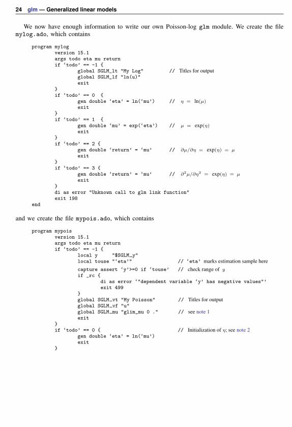
We now have enough information to write our own Poisson-log glm module. We create the filemylog.ado, which contains

program mylogversion 15.1args todo eta mu returnif ‘todo’ == -1 {

global SGLM_lt "My Log" // Titles for outputglobal SGLM_lf "ln(u)"exit

}if ‘todo’ == 0 {

gen double ‘eta’ = ln(‘mu’) // η = ln(µ)exit

}if ‘todo’ == 1 {

gen double ‘mu’ = exp(‘eta’) // µ = exp(η)exit

}if ‘todo’ == 2 {

gen double ‘return’ = ‘mu’ // ∂µ/∂η = exp(η) = µ

exit}if ‘todo’ == 3 {

gen double ‘return’ = ‘mu’ // ∂2µ/∂η2 = exp(η) = µ

exit}di as error "Unknown call to glm link function"exit 198

end

and we create the file mypois.ado, which contains

program mypoisversion 15.1args todo eta mu returnif ‘todo’ == -1 {

local y "$SGLM y"local touse "‘eta’" // ‘eta’ marks estimation sample herecapture assert ‘y’>=0 if ‘touse’ // check range of yif _rc {

di as error ‘"dependent variable ‘y’ has negative values"’exit 499

}global SGLM vt "My Poisson" // Titles for outputglobal SGLM vf "u"global SGLM mu "glim_mu 0 ." // see note 1exit

}if ‘todo’ == 0 { // Initialization of η; see note 2

gen double ‘eta’ = ln(‘mu’)exit

}


if ‘todo’ == 1 {gen double ‘return’ = ‘mu’ // V (µ) = µ

exit}if ‘todo’ == 2 { // ∂ V (µ)/∂µ

gen byte ‘return’ = 1exit

}if ‘todo’ == 3 { // squared deviance, defined above

local y "$SGLM y"if "‘y’" == "" {

local y "‘e(depvar)’"}gen double ‘return’ = cond(‘y’==0, 2*‘mu’, /*

*/ 2*(‘y’*ln(‘y’/‘mu’)-(‘y’-‘mu’)))exit

}if ‘todo’ == 4 { // Anscombe residual; see note 3


local y "‘e(depvar)’"}gen double ‘return’ = 1.5*(‘y’^(2/3)-‘mu’^(2/3)) / ‘mu’^(1/6)exit

}if ‘todo’ == 5 { // log likelihood; see note 4


local y "‘e(depvar)’"}gen double ‘return’ = -‘mu’+‘y’*ln(‘mu’)-lngamma(‘y’+1)exit

}if ‘todo’ == 6 { // adjustment to residual; see note 5

gen double ‘return’ = 1/(6*sqrt(‘mu’))exit

}di as error "Unknown call to glm variance function"error 198

end

Notes:

1. glim mu is a Stata program that will, at each iteration, bring µ back into its plausible range,should it stray out of it. Here glim mu is called with the arguments zero and missing, meaningthat zero is the lower bound of µ and there exists no upper bound—such is the case for Poissonmodels.

2. Here the initial value of η is easy because we intend to fit this model with our user-definedlog link. In general, however, the initialization may need to vary according to the link to obtainconvergence. If so, the global macro SGLM L is used to determine which link is being utilized.

3. The Anscombe formula is given here because we know it. If we were not interested in Anscomberesiduals, we could merely set ‘return’ to missing. Also, the local macro y is set either toSGLM y if it is in current estimation or to e(depvar) if this function is being accessed by predict.

4. If we were not interested in ML estimation, we could omit this code entirely and just leave anexit statement in its place. Similarly, if we were not interested in deviance or IRLS optimization,we could set ‘return’ in the deviance portion of the code (‘todo’==3) to missing.


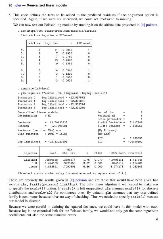
5. This code defines the term to be added to the predicted residuals if the adjusted option isspecified. Again, if we were not interested, we could set ‘return’ to missing.

We can now test our Poisson-log module by running it on the airline data presented in [R] poisson.

. use http://www.stata-press.com/data/r15/airline

. list airline injuries n XYZowned

airline injuries n XYZowned

1. 1 11 0.0950 12. 2 7 0.1920 03. 3 7 0.0750 04. 4 19 0.2078 05. 5 9 0.1382 0

6. 6 4 0.0540 17. 7 3 0.1292 08. 8 1 0.0503 09. 9 3 0.0629 1

. generate lnN=ln(n)

. glm injuries XYZowned lnN, f(mypois) l(mylog) scale(1)




Variance function: V(u) = u [My Poisson]Link function : g(u) = ln(u) [My Log]

AIC = 5.629395Log likelihood = -22.33227605 BIC = -.4790192

OIMinjuries Coef. Std. Err. z P>|z| [95% Conf. Interval]

XYZowned .6840668 .3895877 1.76 0.079 -.0795111 1.447645lnN 1.424169 .3725155 3.82 0.000 .6940517 2.154286

_cons 4.863891 .7090501 6.86 0.000 3.474178 6.253603

(Standard errors scaled using dispersion equal to square root of 1.)

These are precisely the results given in [R] poisson and are those that would have been given hadwe run glm, family(poisson) link(log). The only minor adjustment we needed to make wasto specify the scale(1) option. If scale() is left unspecified, glm assumes scale(1) for discretedistributions and scale(x2) for continuous ones. By default, glm assumes that any user-definedfamily is continuous because it has no way of checking. Thus we needed to specify scale(1) becauseour model is discrete.

Because we were careful in defining the squared deviance, we could have fit this model with IRLS.Because log is the canonical link for the Poisson family, we would not only get the same regressioncoefficients but also the same standard errors.

http://www.stata.com/manuals/rpoisson.pdf#rpoisson



Example 6

Suppose now that we wish to use our log link (mylog.ado) with glm’s binomial family. This taskrequires some modification because our current function is not equipped to deal with the binomialdenominator, which we are allowed to specify. This denominator is accessible to our link functionthrough the global macro SGLM m. We now make the modifications and store them in mylog2.ado.

program mylog2 // <-- changedversion 15.1args todo eta mu return

if ‘todo’ == -1 {global SGLM_lt "My Log, Version 2" // <-- changedif "$SGLM m" == "1" { // <-- changed

global SGLM lf "ln(u)" // <-- changed} // <-- changedelse global SGLM lf "ln(u/$SGLM m)" // <-- changedexit

}if ‘todo’ == 0 {

gen double ‘eta’ = ln(‘mu’/$SGLM m) // <-- changedexit

}if ‘todo’ == 1 {

gen double ‘mu’ = $SGLM m*exp(‘eta’) // <-- changedexit

}if ‘todo’ == 2 {

gen double ‘return’ = ‘mu’exit

}if ‘todo’ == 3 {

gen double ‘return’ = ‘mu’exit

}di as error "Unknown call to glm link function"exit 198

end

We can now run our new log link with glm’s binomial family. Using the flour beetle data fromearlier, we have


. use http://www.stata-press.com/data/r15/beetle, clear

. glm r ldose, f(bin n) l(mylog2) irls

Iteration 1: deviance = 2212.108Iteration 2: deviance = 452.9352Iteration 3: deviance = 429.95Iteration 4: deviance = 429.2745Iteration 5: deviance = 429.2192Iteration 6: deviance = 429.2082Iteration 7: deviance = 429.2061Iteration 8: deviance = 429.2057Iteration 9: deviance = 429.2056Iteration 10: deviance = 429.2056Iteration 11: deviance = 429.2056Iteration 12: deviance = 429.2056

Generalized linear models No. of obs = 24Optimization : MQL Fisher scoring Residual df = 22

(IRLS EIM) Scale parameter = 1Deviance = 429.205599 (1/df) Deviance = 19.50935Pearson = 413.088142 (1/df) Pearson = 18.77673

Variance function: V(u) = u*(1-u/n) [Binomial]Link function : g(u) = ln(u/n) [My Log, Version 2]

BIC = 359.2884

EIMr Coef. Std. Err. z P>|z| [95% Conf. Interval]

ldose 8.478908 .4702808 18.03 0.000 7.557175 9.400642_cons -16.11006 .8723167 -18.47 0.000 -17.81977 -14.40035

For a more detailed discussion on user-defined functions, and for an example of a user-definedNewey–West kernel weight, see Hardin and Hilbe (2018).

� �John Ashworth Nelder (1924–2010) was born in Somerset, England. He studied mathematicsand statistics at Cambridge and worked as a statistician at the National Vegetable ResearchStation and then Rothamsted Experimental Station. In retirement, he was actively affiliated withImperial College London. Nelder was especially well known for his contributions to the theoryof linear models and to statistical computing. He was the principal architect of generalized andhierarchical generalized linear models and of the programs GenStat and GLIM.

Robert William Maclagan Wedderburn (1947–1975) was born in Edinburgh and studied mathe-matics and statistics at Cambridge. At Rothamsted Experimental Station, he developed the theoryof generalized linear models with Nelder and originated the concept of quasilikelihood. He diedof anaphylactic shock from an insect bite on a canal holiday.� �


Stored resultsglm, ml stores the following in e():

Scalarse(N) number of observationse(k) number of parameterse(k eq) number of equations in e(b)e(k eq model) number of equations in overall model teste(k dv) number of dependent variablese(df m) model degrees of freedome(df) residual degrees of freedome(phi) scale parametere(aic) model AICe(bic) model BICe(ll) log likelihood, if NRe(N clust) number of clusterse(chi2) χ2

e(p) p-value for model teste(deviance) deviancee(deviance s) scaled deviancee(deviance p) Pearson deviancee(deviance ps) scaled Pearson deviancee(dispers) dispersione(dispers s) scaled dispersione(dispers p) Pearson dispersione(dispers ps) scaled Pearson dispersione(nbml) 1 if negative binomial parameter estimated via ML, 0 otherwisee(vf) factor set by vfactor(), 1 if not sete(power) power set by link(power #) or link(opower #)e(rank) rank of e(V)e(ic) number of iterationse(rc) return codee(converged) 1 if converged, 0 otherwise


Macrose(cmd) glme(cmdline) command as typede(depvar) name of dependent variablee(varfunc) program to calculate variance functione(varfunct) variance titlee(varfuncf) variance functione(link) program to calculate link functione(linkt) link titlee(linkf) link functione(m) number of binomial trialse(wtype) weight typee(wexp) weight expressione(title) title in estimation outpute(clustvar) name of cluster variablee(offset) linear offset variablee(chi2type) Wald; type of model χ2 teste(cons) noconstant, if specifiede(hac kernel) HAC kernele(hac lag) HAC lage(vce) vcetype specified in vce()e(vcetype) title used to label Std. Err.e(opt) ml or irlse(opt1) optimization title, line 1e(opt2) optimization title, line 2e(which) max or min; whether optimizer is to perform maximization or minimizatione(ml method) type of ml methode(user) name of likelihood-evaluator programe(technique) maximization techniquee(properties) b Ve(predict) program used to implement predicte(marginsok) predictions allowed by marginse(marginsnotok) predictions disallowed by marginse(asbalanced) factor variables fvset as asbalancede(asobserved) factor variables fvset as asobserved

Matricese(b) coefficient vectore(Cns) constraints matrixe(ilog) iteration log (up to 20 iterations)e(gradient) gradient vectore(V) variance–covariance matrix of the estimatorse(V modelbased) model-based variance

Functionse(sample) marks estimation sample


glm, irls stores the following in e():

Scalarse(N) number of observationse(k) number of parameterse(k eq model) number of equations in overall model teste(df m) model degrees of freedome(df) residual degrees of freedome(phi) scale parametere(disp) dispersion parametere(bic) model BICe(N clust) number of clusterse(deviance) deviancee(deviance s) scaled deviancee(deviance p) Pearson deviancee(deviance ps) scaled Pearson deviancee(dispers) dispersione(dispers s) scaled dispersione(dispers p) Pearson dispersione(dispers ps) scaled Pearson dispersione(nbml) 1 if negative binomial parameter estimated via ML, 0 otherwisee(vf) factor set by vfactor(), 1 if not sete(power) power set by link(power #) or link(opower #)e(rank) rank of e(V)e(rc) return code

Macrose(cmd) glme(cmdline) command as typede(depvar) name of dependent variablee(varfunc) program to calculate variance functione(varfunct) variance titlee(varfuncf) variance functione(link) program to calculate link functione(linkt) link titlee(linkf) link functione(m) number of binomial trialse(wtype) weight typee(wexp) weight expressione(clustvar) name of cluster variablee(offset) linear offset variablee(cons) noconstant, if specifiede(hac kernel) HAC kernele(hac lag) HAC lage(vce) vcetype specified in vce()e(vcetype) title used to label Std. Err.e(opt) ml or irlse(opt1) optimization title, line 1e(opt2) optimization title, line 2e(properties) b Ve(predict) program used to implement predicte(marginsok) predictions allowed by marginse(marginsnotok) predictions disallowed by marginse(asbalanced) factor variables fvset as asbalancede(asobserved) factor variables fvset as asobserved

Matricese(b) coefficient vectore(V) variance–covariance matrix of the estimatorse(V modelbased) model-based variance

Functionse(sample) marks estimation sample


Methods and formulasThe canonical reference on GLM is McCullagh and Nelder (1989). The term “generalized linear

model” is from Nelder and Wedderburn (1972). Many people use the acronym GLIM for GLM modelsbecause of the classic GLM software tool GLIM, by Baker and Nelder (1985). See Dobson andBarnett (2008) for a concise introduction and overview. See Rabe-Hesketh and Everitt (2007) formore examples of GLM using Stata. Hoffmann (2004) focuses on applying generalized linear models,using real-world datasets, along with interpreting computer output, which for the most part is obtainedusing Stata.

This discussion highlights the details of parameter estimation and predicted statistics. For a moredetailed treatment, and for information on variance estimation, see Hardin and Hilbe (2018). glmsupports estimation with survey data. For details on VCEs with survey data, see [SVY] varianceestimation.

glm obtains results by IRLS, as described in McCullagh and Nelder (1989), or by maximumlikelihood using Newton–Raphson. The implementation here, however, allows user-specified weights,which we denote as vj for the jth observation. Let M be the number of “observations” ignoringweights. Define

wj =

1 if no weights are specifiedvj if fweights or iweights are specifiedMvj/(

∑k vk) if aweights or pweights are specified

The number of observations is then N =∑j wj if fweights are specified and N = M otherwise.

Each IRLS step is performed by regress using wj as the weights.

Let d2j denote the squared deviance residual for the jth observation:

For the Gaussian family, d2j = (yj − µj)2.

For the Bernoulli family (binomial with denominator 1),

d2j =

{−2ln(1− µj) if yj = 0−2ln(µj) otherwise

For the binomial family with denominator mj ,

d2j =

2yj ln(yj/µj) + 2(mj − yj)ln

{(mj − yj)/(mj − µj)

}if 0 < yj < mj

2mj ln{mj/(mj − µj)

}if yj = 0

2yj ln(yj/µj) if yj = mj

For the Poisson family,

d2j =

{2µj if yj = 0

2{yj ln(yj/µj)− (yj − µj)

}otherwise

For the gamma family, d2j = −2{

ln(yj/µj)− (yj − µj)/µj}

.

For the inverse Gaussian, d2j = (yj − µj)2/(µ2jyj).

http://www.stata.com/manuals/svyvarianceestimation.pdf#svyvarianceestimation

http://www.stata.com/manuals/svyvarianceestimation.pdf#svyvarianceestimation


For the negative binomial,

d2j =

{2ln(1 + kµj)/k if yj = 0

2yj ln(yj/µj)− 2{(1 + kyj)/k}ln{(1 + kyj)/(1 + kµj)} otherwise

Let φ = 1 if the scale parameter is set to one; otherwise, define φ = φ0(n− k)/n, where φ0 is theestimated scale parameter and k is the number of covariates in the model (including intercept).

Let lnLj denote the log likelihood for the jth observation:

For the Gaussian family,

lnLj = −1

2

[{(yj − µj)2

φ

}+ ln(2πφ)

]

For the binomial family with denominator mj (Bernoulli if all mj = 1),

lnLj = φ×

ln{Γ(mj + 1)} − ln{Γ(yj + 1)} − ln{Γ(mj − yj + 1)} if 0 < yj < mj

+(mj − yj) ln(1− µj/mj) + yj ln(µj/mj)

mj ln(1− µj/mj) if yj = 0

mj ln(µj/mj) if yj = mj

For the Poisson family,

lnLj = φ [yj ln(µj)− µj − ln{Γ(yj + 1)}]

For the gamma family, lnLj = −yj/µj + ln(1/µj).

For the inverse Gaussian,

lnLj = −1

2

{(yj − µj)2

yj µ2j

+ 3 ln(yj) + ln(2π)

}

For the negative binomial (let m = 1/k),

lnLj =φ [ ln{Γ(m+ yj)} − ln{Γ(yj + 1)} − ln{Γ(m)}−m ln(1 + µj/m) + yj ln{µj/(µj +m)}]

The overall deviance reported by glm is D2 =∑j wjd

2j . The dispersion of the deviance is D2

divided by the residual degrees of freedom.

The Akaike information criterion (AIC) and Bayesian information criterion (BIC) are given by

AIC =−2 lnL+ 2k

N

BIC = D2 − (N − k) ln(N)

where lnL =∑j wj lnLj is the overall log likelihood.


The Pearson deviance reported by glm is∑j wjr

2j . The corresponding Pearson dispersion is the

Pearson deviance divided by the residual degrees of freedom. glm also calculates the scaled versionsof all of these quantities by dividing by the estimated scale parameter.

Acknowledgmentsglm was written by James Hardin of the Arnold School of Public Health at the University of

South Carolina and Joseph Hilbe of Arizona State University, the coauthors of the Stata Press bookGeneralized Linear Models and Extensions. The previous version of this routine was written byPatrick Royston of the MRC Clinical Trials Unit, London, and coauthor of the Stata Press bookFlexible Parametric Survival Analysis Using Stata: Beyond the Cox Model. The original versionof this routine was published in Royston (1994). Royston’s work, in turn, was based on a priorimplementation by Joseph Hilbe (1944–2017), first published in Hilbe (1993). Roger Newson wrotean early implementation (Newson 1999) of robust variance estimates for GLM. Parts of this entry areexcerpts from Hardin and Hilbe (2018).

ReferencesAkaike, H. 1973. Information theory and an extension of the maximum likelihood principle. In Second International

Symposium on Information Theory, ed. B. N. Petrov and F. Csaki, 267–281. Budapest: Akailseoniai–Kiudo.

Anscombe, F. J. 1953. Contribution of discussion paper by H. Hotelling “New light on the correlation coefficient andits transforms”. Journal of the Royal Statistical Society, Series B 15: 229–230.

Baker, R. J., and J. A. Nelder. 1985. The Generalized Linear Interactive Modelling System, Release 3.77. Oxford:Numerical Algorithms Group.

Basu, A. 2005. Extended generalized linear models: Simultaneous estimation of flexible link and variance functions.Stata Journal 5: 501–516.

Berndt, E. K., B. H. Hall, R. E. Hall, and J. A. Hausman. 1974. Estimation and inference in nonlinear structuralmodels. Annals of Economic and Social Measurement 3/4: 653–665.

Cummings, P. 2009. Methods for estimating adjusted risk ratios. Stata Journal 9: 175–196.

Discacciati, A., and M. Bottai. 2017. Instantaneous geometric rates via generalized linear models. Stata Journal 17:358–371.

Dobson, A. J., and A. G. Barnett. 2008. An Introduction to Generalized Linear Models. 3rd ed. Boca Raton, FL:Chapman & Hall/CRC.

Hardin, J. W., and J. M. Hilbe. 2018. Generalized Linear Models and Extensions. 4th ed. College Station, TX: StataPress.

Hilbe, J. M. 1993. sg16: Generalized linear models. Stata Technical Bulletin 11: 20–28. Reprinted in Stata TechnicalBulletin Reprints, vol. 2, pp. 149–159. College Station, TX: Stata Press.

. 2000. sg126: Two-parameter log-gamma and log-inverse Gaussian models. Stata Technical Bulletin 53: 31–32.Reprinted in Stata Technical Bulletin Reprints, vol. 9, pp. 273–275. College Station, TX: Stata Press.

. 2009. Logistic Regression Models. Boca Raton, FL: Chapman & Hill/CRC.

. 2014. Modeling Count Data. New York: Cambridge University Press.

Hoffmann, J. P. 2004. Generalized Linear Models: An Applied Approach. Boston: Pearson.

Hosmer, D. W., Jr., S. A. Lemeshow, and R. X. Sturdivant. 2013. Applied Logistic Regression. 3rd ed. Hoboken,NJ: Wiley.

McCullagh, P., and J. A. Nelder. 1989. Generalized Linear Models. 2nd ed. London: Chapman & Hall/CRC.

Nelder, J. A. 1975. Robert William MacLagan Wedderburn, 1947–1975. Journal of the Royal Statistical Society, SeriesA 138: 587.

Nelder, J. A., and R. W. M. Wedderburn. 1972. Generalized linear models. Journal of the Royal Statistical Society,Series A 135: 370–384.

http://www.stata-press.com/books/glmext3.html

http://www.stata-press.com/books/fpsaus.html

http://www.stata-journal.com/article.html?article=st0092



http://www.stata-press.com/books/generalized-linear-models-and-extensions/

http://www.stata.com/products/stb/journals/stb11.pdf


http://www.stata.com/bookstore/lrm.html

http://www.stata.com/bookstore/modeling-count-data/

http://www.stata.com/bookstore/glmaa.html

http://www.stata.com/bookstore/applied-logistic-regression/

http://www.stata.com/bookstore/glm.html


Newey, W. K., and K. D. West. 1987. A simple, positive semi-definite, heteroskedasticity and autocorrelation consistentcovariance matrix. Econometrica 55: 703–708.

Newson, R. B. 1999. sg114: rglm—Robust variance estimates for generalized linear models. Stata Technical Bulletin50: 27–33. Reprinted in Stata Technical Bulletin Reprints, vol. 9, pp. 181–190. College Station, TX: Stata Press.

. 2004. Generalized power calculations for generalized linear models and more. Stata Journal 4: 379–401.

Orsini, N., R. Bellocco, and P. C. Sjolander. 2013. Doubly robust estimation in generalized linear models. StataJournal 13: 185–205.

Parner, E. T., and P. K. Andersen. 2010. Regression analysis of censored data using pseudo-observations. Stata Journal10: 408–422.

Pregibon, D. 1980. Goodness of link tests for generalized linear models. Applied Statistics 29: 15–24.

Rabe-Hesketh, S., and B. S. Everitt. 2007. A Handbook of Statistical Analyses Using Stata. 4th ed. Boca Raton, FL:Chapman & Hall/CRC.

Rabe-Hesketh, S., A. Pickles, and C. Taylor. 2000. sg129: Generalized linear latent and mixed models. Stata TechnicalBulletin 53: 47–57. Reprinted in Stata Technical Bulletin Reprints, vol. 9, pp. 293–307. College Station, TX: StataPress.

Rabe-Hesketh, S., A. Skrondal, and A. Pickles. 2002. Reliable estimation of generalized linear mixed models usingadaptive quadrature. Stata Journal 2: 1–21.

Raftery, A. E. 1995. Bayesian model selection in social research. In Vol. 25 of Sociological Methodology, ed. P. V.Marsden, 111–163. Oxford: Blackwell.

Rogers, W. H. 1993. sg16.4: Comparison of nbreg and glm for negative binomial. Stata Technical Bulletin 16: 7.Reprinted in Stata Technical Bulletin Reprints, vol. 3, pp. 82–84. College Station, TX: Stata Press.

Royston, P. 1994. sg22: Generalized linear models: Revision of glm. Stata Technical Bulletin 18: 6–11. Reprinted inStata Technical Bulletin Reprints, vol. 3, pp. 112–121. College Station, TX: Stata Press.

Sasieni, P. D. 2012. Age–period–cohort models in Stata. Stata Journal 12: 45–60.

Schonlau, M. 2005. Boosted regression (boosting): An introductory tutorial and a Stata plugin. Stata Journal 5:330–354.

Senn, S. J. 2003. A conversation with John Nelder. Statistical Science 18: 118–131.

Williams, R. 2010. Fitting heterogeneous choice models with oglm. Stata Journal 10: 540–567.

Also see[R] glm postestimation — Postestimation tools for glm

[R] cloglog — Complementary log-log regression

[R] logistic — Logistic regression, reporting odds ratios

[R] nbreg — Negative binomial regression

[R] poisson — Poisson regression

[R] regress — Linear regression

[BAYES] bayes: glm — Bayesian generalized linear models

[FMM] fmm: glm — Finite mixtures of generalized linear regression models

[ME] meglm — Multilevel mixed-effects generalized linear model

[MI] estimation — Estimation commands for use with mi estimate

[SVY] svy estimation — Estimation commands for survey data

[XT] xtgee — Fit population-averaged panel-data models by using GEE

[U] 20 Estimation and postestimation commands













http://www.stata.com/manuals/rglmpostestimation.pdf#rglmpostestimation

http://www.stata.com/manuals/rcloglog.pdf#rcloglog


http://www.stata.com/manuals/rnbreg.pdf#rnbreg


http://www.stata.com/manuals/rregress.pdf#rregress

http://www.stata.com/manuals/bayesbayesglm.pdf#bayesbayesglm

http://www.stata.com/manuals/fmmfmmglm.pdf#fmmfmmglm

http://www.stata.com/manuals/memeglm.pdf#memeglm

http://www.stata.com/manuals/miestimation.pdf#miestimation

http://www.stata.com/manuals/svysvyestimation.pdf#svysvyestimation

http://www.stata.com/manuals/xtxtgee.pdf#xtxtgee

http://www.stata.com/manuals/u20.pdf#u20Estimationandpostestimationcommands

Documents

glm — Generalized linear models · or Newton–Raphson ... (binomial) Logit model of y events occurring in 15 trials as a function of x glm y x, ... glm— Generalized linear models