Embed Size (px)
Citation preview
Spintronics
R.A. Duine∗
Institute for Theoretical Physics, Utrecht University,Leuvenlaan 4, 3584 CE Utrecht, The Netherlands
(Dated: February 24, 2010)
AbstractThese are lecture notes for the course “spintronics”, taught at Utrecht University, Spring 2009.
∗Electronic address: [email protected]; URL: http://www.phys.uu.nl/~duine
1

R.A. Duine — Spintronics
Contents
I. Introduction 4Additional reading 5
II. Path integrals for spins 6Exercises 91. Action from equation of motion 92. Low-temperature approximation 103. Partition function single spin from path-integral expression 11Additional reading 12
III. Simple models for ferromagnetism 13Landau theory 13Heisenberg model 14Stoner mean-field theory 16
Hubbard model 16Homogeneous Fermi gas 19
Exercises 211. Spin waves — semiclassical approach 212. Spin waves in a S = 1
2Heisenberg chain 21
3. Mean-field theory for the Heisenberg chain revisited 224. Fermi gas 225. Hartree-Fock theory of a Fermi gas at zero temperature 226. Stoner mean-field theory revisited 237. Spin density waves in one and two dimensions 238. Spin waves in an itinerant ferromagnet 24Additional reading 25
IV. Phenomenology of magnetism 26Magnetic anisotropy 26Magnetization dynamics 28Exercises 301. Properties of the Landau-Lifschitz-Gilbert equation 302. Spin waves revisited 303. Magnetization damping 314. Toy-model of magnetization reversal and hysteresis 315. Magnetization damping 316. Determining αG from a ferromagnetic resonance experiment 32Additional reading 33
V. Spin Valves 34Experiment: giant magnetoresistance and spin transfer torques 34Theory 37
s− d model 37Julliere formula 38Spin transfer from conservation of total spin angular momentum 40
Exercises 44
2

R.A. Duine — Spintronics
1. Spin current 442. Critical current and switching 443. Composition rules for two scatterers 444. Transmission coefficient for a simple model of a spin valve 45Additional reading 47
VI. Spin transfer torques for smooth magnetization textures 48Symmetries, conservation laws, and gauge fields 48
Charge conservation: global U(1) symmetry 48U(1) gauge theory 49SU(2): spin and spin currents revisited 51
Spin transfer torques as gauge fields 52Exercises 561. Equation of motion 562. Adiabatic spin transfer torque as a Slonczewski spin transfer torque 56Additional reading 57
VII. Domain Wall Motion 58Domain walls 58Moving domain walls 59
Field-driven domain-wall motion 62Current-driven domain-wall motion 63
Exercises 641. Spin waves with current 642. Domain Wall Mass 64Additional reading 66
VIII. Spin Hall effect 67Exercises 691. Rashba model 69Additional reading 70
IX. Acknowledgements 71
A. Electronic transport 72Landauer-Butikker formalism 72Boltzmann transport theory 72Linear-response theory 76Disorder 77Additional reading 81
3
R.A. Duine — Spintronics
I. INTRODUCTION
According to the Oxford English Dictionary, spintronics is “A branch of physics concernedwith the storage and transfer of information by means of electron spins in addition to electroncharge as in conventional electronics”. Although the emphasis of this reasonable definitionis on applications to information storage, spintronics has, in addition to nano-electronicsengineers and materials scientists, also attracted researchers from the field of (theoretical)condensed-matter physics interested in more fundamental problems. The research field ofspintronics essentially took off with the discovery of giant magnetoresistance (GMR, 2007Nobel prize Grunberg and Fert) in the late 80s/early 90s, which led to a 100× increasein the storage capacity of harddrives less than 10 years later. Since then it has differenti-ated into three closely related themes: i) ferromagnetic metal spintronics, ii) ferromagneticsemiconductor spintronics, and iii) paramagnetic semiconductor spintronics. In the subfieldferromagnetic metal spintronics the focus is on manipulating magnetization with currentand vice versa. Similar phenomena are pursued in ferromagnetic semiconductor spintronics,in addition to achieving a critical temperature well above room temperature. Paramagneticsemiconductor spintronics focuses on spin-orbit coupling effects.
The aim of this course is to provide an introduction to spintronics from a condensed-matter theory point-of-view. The interest of condensed-matter theory in ferromagnetic metaland semiconductor spintronics is motivated by the following reasons. A general theme incondensed matter physics is to achieve a macroscopic low-energy description of a systemstarting from its microscopic hamiltonian. Usually, these systems are at high energies de-scribed in terms of electronic degrees of freedom, whereas at low energies and temperaturesthe system is described in terms of so-called collective degrees of freedom and/or an orderparameter. However, even at low temperatures, say below a critical temperature wherethe system develops a nonzero order parameter, there are still degrees of freedom that areparticle-like in nature. For example, even though the low-energy excitations in a ferromagnetare spin waves, a current in a ferromagnetic metal is carried by the electronic quasiparticles.Because they carry the electric current, these quasiparticles are necessarily out of equilib-rium. From this perspective, ferromagnetic metal and semiconductor spintronics studiesthe interaction between nonequilibrium quasiparticles and collective degrees of freedom —a topic that is extremely interesting for condensed-matter theorists!
The subfield paramagnetic semiconductor spintronics is interesting from a fundamentalpoint of view because spin is not a conserved quantity. Charge, on the other hand, is aconserved quantity in the sense that it always obeys a continuity equation: unless there isa source, the charge in a given volume element can only change by charge flowing in andout of the element. No charge can appear or dissappear. The same is not true for spin.An electron with spin pointing in the, say, z-direction can encounter a magnetic impuritythat changes its spin to the x-direction. So, the spin in the z-direction is not conservedin this example. Another interesting feature of spin currents is that they can in principleoccur without any charge current. Consider the case that all the “up” electrons move inone direction, and that all the “down” electrons move in the opposite direction. In the casethat the material is paramagnetic, i.e., nonmagnetic, there will be a pure spin current butno charge current. This situation occurs in the spin Hall effect: a charge current lead to apure spin current in the direction perpendicular to it.
From the above it is clear that understanding spintronics requires understanding of ferro-magnetism and electron transport, and of combining them. With this in mind, these lectures
4

R.A. Duine — Spintronics
cover the following main topics:
• magnetism
• electron transport
• spin transfer torques: interaction between magnetization and electron transport
• spin Hall effect: effects of spin-orbit coupling
Additional reading
A regularly-cited review paper is:
• S.A. Wolf et al., Science 294, 1488 (2001).
5
R.A. Duine — Spintronics
II. PATH INTEGRALS FOR SPINS
Consider a (localized) spin S, with the total angular momentum quantum number S
positive and integer or half integer. Quantummechanically, it is described by operators Sα,with α ∈ x, y, z, that obey the angular-momentum commutation relations
[Sα, Sβ
]= i~εαβγSγ , (1)
where a summation over repeated indices is implied. The operators Sα commute with S2.As a basis for the Hilbert space one conventionally takes the 2S +1 simultaneous eigenstatesof S2 and Sz:
S2|S; mS〉 = S(S + 1)~2|S; mS〉 ;
Sz|S; mS〉 = mS~|S; mS〉, mS ∈ −S,−S + 1, . . . , S − 1, S . (2)
The hamiltonian H = H[S] is given in terms of the operators Sα. For example, a spin in amagnetic field is described by the hamiltonian
H[S] = −gB · S , (3)
with g a positive constant.The canonical partition function is defined by
Z = Tr[e−βT H[S]
], (4)
with βT = 1/(kBT ) the inverse thermal energy. The trace is over the entire Hilbert space.The goal of this chapter is to find a path-integral expression for this partition function. Weproceed in the usual way, and interpret the exponential in Eq. (4) as an evolution operatorin imaginary time, from τ = 0 to τ = ~βT . We divide this imaginary-time interval intoinfinitesimal pieces ∆τ = ~βT /N , with N large. Up to first order in ∆τ we have for thepartition function
Z = Tr[e−
∑N−1j=0 ∆τH[S]/~
]
= Tr[(
1−∆τH[S]/~)(
1−∆τH[S]/~)· · ·
(1−∆τH[S]/~
)]. (5)
To make progress towards a path-integral expression for Z we would like to get rid of theoperators in this expression. This is usually achieved by inserting complete sets of states inbetween the products in Eq. (5). Therefore, we would like to construct states such that
S|Ω〉 = ~SΩ|Ω〉 , (6)
with Ω a unit vector. This turns out to be impossible. However, it turns out that thereexist so-called spin coherent states that have the property that
〈Ω|S|Ω〉 = ~SΩ . (7)
6

R.A. Duine — Spintronics
We introduce a parameterization for the unit vector Ω in terms of polar coordinates θ ∈ [0, π)and φ ∈ [0, 2π) given by
Ω =
sin θ cos φsin θ sin φ
cos θ
. (8)
Without proof we state some properties of the spin coherent states |Ω〉. They are, up to aphase factor, explicitly given by
|Ω〉 =
mS=S∑mS=−S
(2S
S + mS
) 12
e−i(mS−S)φ
(cos
θ
2
)S+mS(
sinθ
2
)S−mS
|S; mS〉 . (9)
It follows that their overlap is given by
〈Ω′|Ω〉 =
[cos
θ′
2cos
θ
2+ sin
θ′
2sin
θ
2ei(φ−φ′)
]2S
, (10)
so that for infinitesimally separated states we have
〈Ω′|Ω〉 = 1 + iS(φ′ − φ)(cos θ − 1) . (11)
Moreover, they obey the closure relation(
2S + 1
4π
) ∫dΩ|Ω〉〈Ω| = 1 , (12)
where the integral measure∫
dΩ =∫ 1
−1d(cos θ)
∫ 2π
0dφ.
Using this closure relation we find that the trace of an operator O is given by
Tr[O
]=
(2S + 1
4π
) ∫dΩ〈Ω|O|Ω〉 . (13)
By inserting the closure relation in Eq. (12) between the factors in the product in Eq. (5)we find, using the above expression for the trace of an operator, that
Z =
(2S + 1
4π
)N(
N−1∏j=0
∫dΩj
)〈Ω0|
(1−∆τH[S]/~
)|ΩN−1〉
〈ΩN−1|(1−∆τH[S]/~
)|ΩN−2〉 · · · 〈Ω1|
(1−∆τH[S]/~
)|Ω0〉 . (14)
We have, using the defining property in Eq. (7), that
〈Ωj+1|(1−∆τH[S]/~
)|Ωj〉 ' (1−∆τH[~SΩj]/~+ iS(φj+1 − φj)(cos θj − 1))+O(∆τ 2) .
(15)Next, we write these factors as an exponential which is valid up to O(∆τ) , so that we havethat
Z =
(2S + 1
4π
)N(
N−1∏j=0
∫dΩj
)[e−∆τH[~SΩN−1]/~+iS(φ0−φN−1)(cos θN−1−1)
]
[e−∆τH[~SΩN−2]/~+iS(φN−1−φN−2)(cos θN−2−1)
] · · · [e−∆τH[~SΩ0]/~+iS(φ1−φ0)(cos θ0−1)]
. (16)
7

R.A. Duine — Spintronics
This expression is rewritten as
Z =
(2S + 1
4π
)N(
N−1∏j=0
∫dΩj
)
× exp
N∑
j=0
∆τ
[iS
(φj+1 − φj
∆τ
)(cos θj − 1)− H[~SΩj]
~
], (17)
where periodic boundary conditions φ0 = φN and θ0 = θN are assumed. Finally, we takethe continuum limit N →∞, ∆τ → 0, with N∆τ = ~βT fixed. Using the notation
τ = j∆τ
φj → φ(τ) ;
θj → θ(τ) ;
∆τ → dτ ;
φj+1 − φj
∆τ→ dφ(τ)
dτ≡ φ(τ) ;
(2S + 1
4π
)N(
N−1∏j=0
∫dΩj
)→ DΩ(τ) , (18)
we find that the partition function is given as a path integral over all periodic paths Ω(τ)on the unit sphere:
Z =
∫
Ω(0)=Ω(~βT )
DΩ(τ) exp
−1
~AE[Ω]
. (19)
In this expression, the Euclidean action is given by
AE[Ω] =
∫ ~βT
0
dτ
i~Sφ(τ) [1− cos θ(τ)] + H[~SΩ(τ)]
, (20)
and consists of the usual potential term involving the hamiltonian, as well as a kinetic termsthat give rise to a phase factor
e−iS∫ ~βT0 dτφ(τ)[1−cos θ(τ)] , (21)
which is called a geometric phase, or Berry phase, since it depends only on the trajectoryon the unit sphere and not explicitly on the time dependence. This is seen by realizing that
∫ ~βT
0
dτφ(τ) [1− cos θ(τ)] =
∫ φ0
φ0
dφ (1− cos θφ) . (22)
The right-hand side of this equation is in fact the area A on the unit sphere that is enclosedby the trajectory (cos φ(τ) sin θ(τ), sin φ(τ) sin θ(τ), cos θ(τ)) on the unit sphere. Withoutexplicitly choosing a parameterization for Ω we can also write this area as a surface integralover a vector field B(Ω) = Ω:
A =
∫
A
dΩ ·B(Ω) . (23)
8

R.A. Duine — Spintronics
With the use of Stokes theorem we rewrite this surface integral as a line integral over theedge ∂A of the area A
A =
∫
∂A
d` ·A(Ω) =
∫ ~βT
0
dτA(Ω(τ)) · Ω(τ) , (24)
where A(Ω) is the vector potential of a magnetic monopole in Ω-space determined by
∇Ω ×A(Ω) = Ω . (25)
The gauge freedom A(Ω) → A(Ω)−∇ΩΛ(Ω), with Λ(Ω) an arbitrary scalar function, canbe traced back to the arbitrary definition of the phase of the spin coherent states in Eq. (9).Using these results, the Euclidean action is written as
AE[Ω] =
∫ ~βT
0
dτ
[i~SA(Ω(τ)) · ∂Ω
∂τ+ H[~SΩ(τ)]
]. (26)
In Exercise II 1 it is shown that this form of the action indeed leads to the correct semiclas-sical equation of motion [Eq. (30)]. Depending on the application at hand, either the aboveform of the Euclidean action is used or a “gauge-fixed” expression like Eq. (20).
Finally we note that the area that is enclosed by a contour on a unit sphere is definedonly modulo 4π, i.e., if ∫
∂A
d` ·A(Ω) = A (27)
is the area enclosed “on the left” of the contour, then an alternative would be
∫
∂A
d` ·A(Ω) = −(4π − A) , (28)
where the additional minus sign comes from the fact that this area is now negatively orientedwith respect to the contour, i.e., is “on the right” of the contour. In order for the path integralexpression to be unambiguously defined we need to have that
e−iSA = e−iS(A−4π) , (29)
so that S can take only half-integer or integer values . This constitutes a “proof” that thetotal angular momentum quantum number S can take only half-integer or integer values.
Exercises
1. Action from equation of motion
Consider a spin S in an external time-independent magnetic field B. Assume that thehamiltonian of the system is given by
H = −gB · S .
9
R.A. Duine — Spintronics
a) Show, using the spin commutation relations
[Sα, Sβ
]= i~εαβγSγ ,
where a sum over repeated Greek indices α, β, γ ∈ x, y, z is implied and εαβγ isthe antisymmetric Levi-Civita tensor, that the equation of motion for the expectationvalue of the spin is
d
dt〈S〉(t) = g〈S〉(t)×B . (30)
The goal of this exercise is to find an action that, upon variation, reproduces the equationof motion in Eq. (30).
b) We write 〈S〉 = ~SΩ with Ω · Ω = 1. Argue that the Lagrangian L(t) defined byA =
∫dtL(t), where A is the action, is of the form
L(t) = ~S−dΩα
dtAα[Ω] + gBαΩα
.
c) Show that the equation of motion is given by
FαβdΩβ
dt= gBα ,
and give the expression for Fαβ.
d) Motivate the educated guess that Fαβ = εαβγΩγ.
e) Show that this form of Fαβ leads to the correct equation of motion in Eq. (30).
Hint: Remember the length constraint on Ω. Furthermore, you may wish to use thatεαβγεαβ′γ′ = δββ′δγγ′ − δβγ′δβ′γ. Alternatively, one can use A× (B×C) = B(A ·C)−C(A ·B)
f) Show that∇Ω ×A(Ω) = Ω . (31)
g) Perform a Wick rotation t → −iτ , and derive the Euclidian action AE[Ω] by demand-ing that
i
~A[Ω] → −1
~AE[Ω] .
2. Low-temperature approximation
Consider a spin S in a magnetic field B, with Hamiltonian
H = −gB · S .
a) Give the energy eigenvalues of the hamiltonian.
10

R.A. Duine — Spintronics
The path-integral expression for the partition function is given by
Z =
∫DΩ(τ) exp
−1
~
∫ ~βT
0
dτ
[i~SA(Ω(τ)) · ∂Ω
∂τ− g~SB ·Ω
],
where the path integral is over all periodic paths Ω on the unit sphere. The vector potentialobeys the equation
∇Ω ×A(Ω) = Ω .
b) Write Ω ' (δΩx, δΩy, 1 − δΩ2x/2 − δΩ2
y/2). Show that A ' 1/2(−δΩy, δΩx, 0) obeysEq. (31) close to z. Give the action up to second order in δΩα.
c) We define an effective action by means of
Z =
∫DδΩxDδΩy exp
−1
~AE[δΩx, δΩy]
≡
∫DδΩy exp
−1
~Aeff
E [δΩy]
.
Show that the effective action is that of a particle in a harmonic potential. The positionof the particle is δΩy. Give its mass m, and the frequency ω.
d) Using the expressions for m and ω give the eigenvalues of the harmonic oscillator, aswell as the partition function.
e) In which regime is this expression for the partition function a good approximationfor the partition function of a spin S in an external field? Relate your answer to theapproximation in part b) of this exercise.
3. Partition function single spin from path-integral expression
Consider a spin S in a magnetic field B, with Hamiltonian
H = −gB · S .
a) Give the partition function as a discrete and finite sum.
The goal of this exercise is to re-derive this result using path integrals. The path-integralexpression for the partition function is given by
Z =
∫DΩ(τ) exp
−1
~
∫ ~βT
0
dτ
[i~SA(Ω(τ)) · ∂Ω
∂τ− g~SB ·Ω
],
where the path integral is over all periodic paths Ω on the unit sphere.
b) Parametrize Ω = (cos φ sin θ, sin φ sin θ, cos θ), and choose A(Ω) = tan(θ/2)φ. Showthat this choice corresponds to the vector potential of a magnetic monopole as inEq. (31). Choose B in the z-direction. Give the path integral and action in terms ofthe coordinates θ(τ) and φ(τ).
Hint: remember vector calculus! Note that the final result is given in Eq. (20).
c) Integrate the time derivative by parts. Note that the requirement of periodic boundaryconditions φ(0) = φ(~βT ) + 2πn introduces a discrete sum over n.
11
R.A. Duine — Spintronics
d) Introduce the variable u = cos θ. Show that performing the path integration over φ(τ)leads to the constraint that du/dτ = 0. This effectively reduces the path integrationover u to a normal integration.
e) Carry out the sum over n using the Poisson resummation formula given by
∑n
e2πinx =∑
k
δ(k − x) ,
where k, n are integers.
f) Carry out the integration over u to obtain the expression for Z.
Additional reading
A standard textbook reference on the topic of path integrals for spins is
• A. Auerbach, Interacting Electrons and Quantum Magnetism (Springer-Verlag, NewYork, 1994).
A nice paper using path-integrals for spins is:
• H.-B. Braun and D. Loss, Phys. Rev. B 53, 3237 (1996).
I found these lecture notes very useful:
• S. M. Girvin, The Quantum Hall Effect: Novel Excitations and Broken Symmetries,available at: http://www.arxiv.org/abs/cond-mat/9907002.
12

R.A. Duine — Spintronics
III. SIMPLE MODELS FOR FERROMAGNETISM
Magnetism is a very rich topic and we postpone a discussion of the phenomenology ofmagnetism to the next section. The aim of this section is to present two simple modelsthat describe, at the mean-field level, a transition from a nonmagnetic to a spontaneouslymagnetized state. This is the defining property of ferromagnetic materials. The first model isthe so-called Heisenberg model that consists of localized spins that interact with an exchangeinteraction that favors alignment of the spins. The second model, often called Stoner model,is that of electrons with repulsive interactions. Since in the latter model the spins arenot localized the model is said to exhibit itinerant ferromagnetism. First we give a briefintroduction to the Landau theory of ferromagnetic phase transitions.
Landau theory
In the Landau theory of phase transitions the partition function is written as a functionalintegral
Z =
∫d[m]e−βT NfL[m] , (32)
where N is the number of sites in a discrete system, e.g. a lattice with localized spins, andfL[m] is the Landau free energy. For a continuous system with volume V we have that
Z =
∫d[m]e−βT V fL[m] , (33)
where fL[m] is now the Landau free energy density. The distinction between free energyand free energy density is not so important and we will use the term free energy throughoutthe following.
The free energy can be constructed from symmetry arguments. For the models we are go-ing to consider the order parameter m, called the magnetization, is related to the expectationvalue of spin operators. Since under time reversal S → −S, we have that fL[m] = fL[−m]since fL[m] needs to be even under time reversal as it is an energy. (Note that this is onlytrue in the absence of an external magnetic field.) Furthermore, for a system that is invari-ant under spin rotations we require that fL[m] = fL[Rm], where R is a three-dimensionalrotation matrix. Finally, if the system has inversion symmetry only terms even in ∇·m canoccur in the Landau free energy.
From these requirements we find that
fL[m] ∝∫
dx[J(T )(∇ ·m)2 + α(T )m2 + β(T )m4 + · · ·] , (34)
where J(T ), α(T ), β(T ) are coefficients that can depend on temperature and we assume thatwe are sufficiently close to the transition so that m is small and that higher-order terms inm can be neglected.
To describe the transition it is sufficient to consider homogeneous configurations of m sothat
fL[m] ∝ α(T )m2 + β(T )m4 + · · · . (35)
The idea is that the configurations for which fL[m] has a minimum contribute most to thepartition function. Because of spin rotation invariance there will be a continuous set of
13
R.A. Duine — Spintronics
these minima. It turns out that in the thermodynamic limit we should only consider oneof these minima since, roughly speaking, the system will take an infinitely long time todynamically go from one local minimum to another. This is the principle of spontaneoussymmetry breaking: the Landau free energy has certain continuous symmetries, in this casesymmetry under rotation of the magnetization. However, below the critical temperature thesystem picks out one direction in which the magnetization 〈m〉 6= 0. Spontaneous symmetrybreaking leads to the existence of gapless, i.e., zero-energy excitation below the transition.These excitations are called Goldstone modes and correspond, in the case of ferromagnets,to long-wavelength spin waves (also called magnons).
For the free energy in Eq. (35) the critical temperature is determined by α(TC) = 0,provided β(T ) and coefficients of higher order terms are positive as α(T ) changes sign.Above the critical temperature α(T ) > 0 and there is only one energy minimum 〈m〉 = 0which obeys ∂fL[〈m〉]/∂m = 0. Below the critical temperature α(T ) < 0 and there is acontinuous set of minima 〈m〉 6= 0 determined by ∂fL[〈m〉]/∂m = 0.
Note that in the above we assume that the transition from a nonmagnetic is secondorder, i.e., the magnetization 〈m〉 changes continuously from a zero to nonzero value as thetemperature is lowered below TC . Experimentally it is found that first-order ferromagneticphase transitions do exist, especially at low temperature. In the models that we consider inthis section however, the transition to the magnetic state is, at least at the mean-field level,second order in character.
Heisenberg model
The hamiltonian for the Heisenberg model consists of localized spins on a lattice and isgiven by
H[S] = −∑
jk
Jjk
2~2S2Sj · Sk , (36)
where the exchange constants Jjk > 0 so that the system can gain energy by aligning spins(note that in the above energy the Jjk have dimension energy). An interaction betweenspins of the above from is called an exchange interaction. The lattice sites are labelled byj. Note also that Jjk = Jkj and Jjj = 0.
The partition function is given as a path integral
Z =
∫d[Ω] exp
−1
~
∫ ~βT
0
dτ
[∑j
i~SA(Ωj(τ)) · ∂Ωj(τ)
∂τ−
∑
jk
Jjk
2Ωj(τ) ·Ωk(τ)
].
(37)Next, we perform a so-called Hubbard-Stratonovich transformation which amounts in thepresent case to multiplying the partition function with a factor one written as
1 ∝∫
d[m] exp
−1
~
∫ ~βT
0
dτ
[1
2
∑
jk
(mj(τ)−
∑
l
JljΩl(τ)
)J−1
jk
(mk(τ)−
∑m
JkmΩm(τ)
)],
(38)where J−1
jk is the matrix inverse of Jjk so that
∑
l
JjlJ−1lk = δjk . (39)
14
R.A. Duine — Spintronics
The Hubbard-Stratonovich transformation introduces the field mj(τ) which has the expec-tation value
〈mj(τ)〉 =
⟨∑
k
JjkΩk(τ)
⟩. (40)
From this we see that a nonzero 〈mj〉 acts as a mean field due to all other spins, that thespin at site j feels:
Hmf [S] = − 1
~S∑
j
〈mj〉 · Sj . (41)
It will turn out that m is the order parameter for the phase transition.The advantage of the Hubbard-Stratonovich procedure is that the action is now local in
terms of the fields Ωj(τ), i.e., the partition function is given by
Z =
∫d[Ω]d[m] exp
−1
~
∫ ~βT
0
dτ
[1
2
∑
jk
J−1jk mj(τ) ·mk(τ)
−∑
j
(Ωj(τ) ·mj(τ)− i~SA(Ωj(τ)) · ∂Ωj(τ)
∂τ
)]. (42)
To determine the critical temperature we consider only static and homogeneous configura-tions of the magnetization mj(τ) = m. Then the path integral over Ωj(τ) gives N timesthe partition of a spin in a magnetic field m. Hence, we find for the partition function
Z =
∫d[m] exp
−βTm2
2
∑
jk
J−1jk
[ZS(|m|)]N ≡
∫d[m]e−βT NfL[m] , (43)
where N is the number of sites and the partition function of a single spin is given by
ZS(|m|) =S∑
mS=−S
e−βT |m|mS
S . (44)
As an example we take S = 1/2 so that the partition function is, up to irrelevant prefactorsthat lead to constant terms in the Landau free energy, given by
ZS(|m|) ∝ cosh (βT |m|) . (45)
Using this result we find for the Landau free energy
fL[m] =m2
2N
∑
jk
J−1jk − 1
βT
log [cosh (βT |m|)] . (46)
For small |m| this becomes
fL[m] = α(T )m2 +O (|m|4) , (47)
with
α(T ) =1
2
[1
N
∑
jk
J−1jk − βT
]. (48)
15

R.A. Duine — Spintronics
The critical temperature is determined from α(TC) = 0. This gives, using that the systemhas translational invariance,
1
N
∑
jk
J−1jk = βTC
;
⇒ 1
N
∑j
(∑
k
J−1jk
)= βTC
;
⇒∑
k
J−1jk = βTC
;
⇒∑
j
∑
k
JljJ−1jk = βTC
∑j
Jlj ;
⇒∑
k
δkl = 1 = βTC
∑j
Jlj , (49)
so that the critical temperature is determined by
kBTC =∑
k
Jjk . (50)
For a S = 1/2 Heisenberg model with nearest-neighbor interaction Jjk = J(δj,k−1 + δj,k+1)and we find that kBTC = zJ , where z is the number of nearest neighbors.
This latter results are in agreement with our physical intuition: if the thermal energyexceeds the energy gain for aligning neighboring spins, the spin will be pointing in differentdirections at different positions and the average magnetization will be zero. For smalltemperature the spins point on average in the same direction and the magnetization isnonzero.
Stoner mean-field theory
In this section we discuss ferromagnetism in an interacting electron system in three di-mensions. We consider the case of the Hubbard model first, and then briefly discuss thegeneralization to the homogeneous case.
Hubbard model
The Hubbard model is a so-called tight-binding model of electrons, with a repulsiveinteraction parameterized by a constant U > 0. Its hamiltonian is given by
H[c†, c] = −∑
j,j′;σ
tj,j′ c†j,σ cj′,σ + U
∑j
c†j,↑c†j,↓cj,↓cj,↑ . (51)
The operators c†j,σ create an electron at site j with spin σ ∈ ↑, ↓. Their complex conjugates
annihilate an electron. We have the commutation relation[cj,σ, c
†j′,σ′
]= δj,j′δσ,σ′ . The
hopping is between nearest neighbors only so that
tj,j′ = t∑
α=x,y,z
(δj,j′−eαa + δj,j′+eαa) , (52)
16

R.A. Duine — Spintronics
where eα are unit lattice vectors in the α-th direction and t > 0. The lattice constant isdenoted by a. Using the Fourier transform
cj,σ =1√N
∑
k
ck,σe−ik·xj , (53)
where xj denotes lattice site vectors, N is the number of lattice sites and the momentumsummation is over the first Brillouin zone. We find for the noninteracting part of thehamiltonian that
H[c†, c] =∑
k,σ
εkc†k,σ ck,σ , (54)
with the single-electron dispersion
εk = −2t∑
α
cos(kαa) , (55)
where we used that∑
j e−i(k−k′)·xj = Nδk,k′ .The partition function of the system is given as a Grassmann coherent-state path integral
by
Z =
∫d[φ∗]d[φ]e−AE [φ∗,φ]/~ , (56)
with the Euclidean action
AE[φ∗, φ] =
∫ ~βT
0
dτ
∑j,σ
φ∗j,σ(τ)
(~
∂
∂τ− µ
)φj,σ(τ) + H[φ∗(τ), φ(τ)]
, (57)
and µ the chemical potential. We rewrite the interaction term as
Uφ∗j,↑(τ)φ∗j,↓(τ)φj,↓(τ)φj,↑(τ) =U
4
[∑σ
φ∗j,σ(τ)φj,σ(τ)
]2
−U
4
[∑
σ,σ′φ∗j,σ(τ)τσ,σ′ ·Ωj(τ)φj,σ′(τ)
]2
,
(58)with Ωj(τ) an arbitrary unit vector denoting the quantization axis. Functional integrationover the latter enforces rotational invariance. The Pauli matrices are given by
τx =
(0 11 0
), τ y =
(0 −ii 0
), τ z =
(1 00 −1
). (59)
We decouple the two interaction terms in the above expression using a Hubbard-Stratonovich transformation to the fields ρj(τ) and mj(τ), respectively. On aver-age these fields are related to the spin density and number density, i.e., 〈mjΩj〉 =〈∑σ,σ′ φ
∗j,στσ,σ′φj,σ′〉/2 and 〈ρj〉 = 〈φ∗j,↑φj,↑ + φ∗j,↓φj,↓〉. After the transformation we have
that
AE[φ∗, φ, ρ,m] =
∫ ~βT
0
dτ
∫ ~βT
0
dτ ′∑
j,σ;j′,σ′φ∗j,σ(τ)
[−~G−1j,σ;j′,σ′(τ, τ
′)]φj′,σ′(τ
′)
+
∫ ~βT
0
dτ∑
j
[Um2
j(τ)− Uρ2j(τ)
4
], (60)
17
R.A. Duine — Spintronics
where the Green’s function is determined from
G−1j,σ;j′,σ′(τ, τ
′) = −1
~
[(~
∂
∂τ− µ +
Uρj(τ)
2
)δj,j′ − tj,j′
]δσ,σ′ − Umj(τ) · τσ,σ′δj,j′
δ(τ − τ ′)
≡ (G0)−1j,σ;j′,σ′ (τ, τ
′)− Σj,σ;j′,σ′(τ, τ′) , (61)
and the self-energy reads
Σj,σ;j′,σ′(τ, τ′) = −1
~
[Uρj(τ)
2δσ,σ′ − Umj(τ) · τσ,σ′
]δj,j′δ(τ − τ ′) . (62)
After carrying out the functional integration over the electron field we are left with theeffective action
Aeff [ρ,m] =
∫ ~βT
0
dτ∑
j
[Um2
j(τ)− Uρ2j(τ)
4
]− ~Tr
[ln
(−G−1)]
=
∫ ~βT
0
dτ∑
j
[Um2
j(τ)− Uρ2j(τ)
4
]− ~Tr
[ln
(−G−10
)]
+~∞∑
m=1
1
mTr [(G0Σ)m] . (63)
We substitute ρj(τ) = 〈ρ〉 + δρj(τ) and expand in terms of δρj(τ) and mj(τ). Putting theterms linear in δρj(τ) equal to zero gives the Hartree-Fock expression for the total density
〈ρ〉 =∑
σ
Gj,σ;j,σ(τ, τ+) , (64)
with τ+ = τ + η with η ↓ 0.We absorb the Hartree-Fock mean field shift in the chemical potential by renormalizing
µ − U〈ρ〉/2 → µ and focus from now on on the field m. Up to quadratic order in thesefields, the action is given by
Aeff [m] =
∫ ~βT
0
dτ∑
j
Um2
j(τ) +U2
~
∫ ~βT
0
dτ ′∑
j′,a∈x,y,zma
j (τ)Gjj′(τ, τ′)Gj′j(τ
′, τ)maj′(τ
′)
,
(65)with
Gjj′(τ, τ) =1
~βT N
∑
k,n
−~−i~ωn + εk − µ
eik·(xj−xj′)−iωn(τ−τ ′) . (66)
In this expression the ωn are the odd Matsubara frequencies. Considering configurationsconstant in space and time gives, after carrying out the Matsubara summation,
Aeff [m] = ~βT N
[U + U2 1
N
∑
k
∂
∂εkN (εk − µ)
]m2 ≡ ~βT NfL[m] , (67)
18

R.A. Duine — Spintronics
where N(x) = [eβT x + 1]−1 is the Fermi distribution function. We have that N(x) =1/(~βT )
∑n[iωn−x/~]−1 if we assume an appropriate convergence factor. The transition to
the polarized state is determined by ∂fL/∂m = 0, which leads to
U
N
∑
k
∂
∂εkN (εk − µ) < −1 . (68)
At low temperatures we have that N(ε − εF ) → θ(εF − ε), where θ(x) is the Heavisidestep function and where the Fermi energy εF is by definition the chemical potential at zerotemperature determined from the density of electrons. From the above expression we thenfind that
U
N
∑
k
∂
∂εkN (εk − µ) = U
∫dεν(ε)
∂N(ε− µ)
∂ε< −1, (69)
where we introduced the density of states
ν(ε) =1
N
∑
k
δ(εk − ε) . (70)
Using that dθ(x)/dx = δ(x), with δ(x) the delta function we have that
Uν(εF ) > 1 , (71)
which is known as Stoner’s criterion. We now give a brief outline of the same manipulationsfor a continuum model.
Homogeneous Fermi gas
In this section we model the electrons as a Fermi gas with repulsive delta function inter-actions. The hamiltonian is given by
H[ψ†, ψ] =
∫dx
∑σ
ψ†σ(x)
(−~
2∇2
2m
)ψσ(x) + g
∫dxψ†↑(x)ψ†↓(x)ψ↓(x)ψ↑(x) , (72)
with g > 0. The Euclidean action is now given by
AE[φ∗, φ] =
∫ ~βT
0
dτ
∫dx
∑σ
φ∗σ(x, τ)
(~
∂
∂τ− µ
)φσ(x, τ) + H[φ∗(τ), φ(τ)]
. (73)
We perform now essentially the same steps as before. We rewrite the interaction accordingto Eq. (58) and introduce two Hubbard-Stratonovich fields that are on average equal to thelocal spin density and local density:
〈m(x, τ)〉 =
⟨∑
σ,σ′φ∗σ(x, τ)
τσ,σ′
2φσ′(x, τ)
⟩;
〈ρ(x, τ)〉 =⟨φ∗↑(x, τ)φ↑(x, τ) + φ∗↓(x, τ)φ↓(x, τ)
⟩. (74)
19
R.A. Duine — Spintronics
We ignore the mean-field shift and absorb it in the chemical potential as was done previously.The partition function is then given as a path integral by means of
Z =
∫d[φ∗]d[φ]d[m]e−AE [φ∗,φ,m]/~ . (75)
We note explicitly that the functional integration over m consists of an integration of theamplitude |m| and integration over the direction of m on the unit sphere. The Euclideanaction is given by
AE[φ∗, φ,m] =
∫ ~βT
0
dτ
∫dx
∑σ
φ∗σ(x, τ)
(~
∂
∂τ− ~
2∇2
2m− µ
)φσ(x, τ)
+gm2(x, τ)− g∑
σ,σ′φ∗σ(x, τ)m(x, τ) · τσ,σ′φσ′(x, τ)
. (76)
Note that this is essentially the action of electrons exchange-coupled to a magnetic field in thedirection m(x, τ). Below the ferromagnetic transition temperature this effective magneticfield, the so-called exchange field, is nonzero.
The transition temperature is now determined by [compare Eq. (68)]
g
∫dk
(2π)3
∂N(εk − µ)
∂εk< −1 , (77)
where the free-electron dispersion is εk = ~2k2/(2m). At zero temperature the result is givenby
mg(3π2n)1/3
~2> 2π2 , (78)
with n the total density. At small nonzero temperatures the result for the transition tem-perature turns out to be
kBTC
εF
' 2√
6
π3/2
√mgkF
4π~2− π
2, (79)
where kF is the fermi wave number for the nonmagnetic state. Note that these results arecompletely different from the Heisenberg model, which always has nonzero magnetization atzero temperature (at least within mean-field theory). As seen from Eq. (78), at zero temper-ature the interactions still need to be sufficiently strong for the system to have spontaneousmagnetization. From Eq. (79) we observe that the critical temperature goes to zero at thepoint determined by Eq. (78). For weaker interactions there is no transition to a magneticstate anymore. This zero-temperature critical point is called a quantum critical point, andthe associated transition a quantum phase transition.
Stoner’s criterion in Eq. (71), or equivalently Eq. (78), describes the competition betweeninteractions and kinetic energy. In the fully-polarized state the interaction energy is zero inthe simple models of Eq. (51) and (72). The kinetic energy of this state however is largerbecause the radius of the Fermi sphere of the polarized state is a factor 21/3 larger than theunpolarized state. Note that this argument shows that the Pauli exclusion principle plays acrucial role in itinerant ferromagnetism.
We end this section with a few remarks for caution. The transition point determined bythe Stoner criterion turns out to the a strong-coupling point, i.e., the interactions are strong
20

R.A. Duine — Spintronics
and the mean-field theory approach of this section is, in principle, not valid. Nonetheless,the results turn out to provide at least a reasonable qualitative picture of the dynamics ofan itinerant ferromagnet. Also note that the hamiltonian in Eq. (72) leads to ultravioletdivergencies and therefore needs to be interpreted as an effective hamiltonian.
Exercises
1. Spin waves — semiclassical approach
The real-time action for the nearest-neighbor Heisenberg model is given by
A[Ω] =
∫dt
∑
j
−~SA(Ωj(t)) · ∂Ωj(t)
∂t+
J
2
∑
〈jk〉Ωj(t) ·Ωk(t)
, (80)
where the notation 〈· · ·〉 indicates that the sum is over nearest neighbors only.
a) Give the equation of motion for Ωj(t)
b) Choose the ground-state magnetization in the z-direction and linearize around thishomogeneous state by means of Ωj(t) ' (δΩx
j (t), δΩyj (t), 1), i.e., give the equations of
motion to linear order in δΩα(t).
c) Consider one dimension and perform a Fourier analysis to find the dispersion relation.Denote the lattice constant by a.
d) Write the dispersion relation as ~ωk = Jsk2 at long wavelengths and give the expression
for the so-called spin stiffness Js.
e) Add a magnetic field in the z-direction and show that the dispersion becomes gapped.Give a physical explanation for this result.
The rest of this exercise we take J < 0 so that the ground state is antiferromagneticallyordered, i.e., Ωj = (−)j(0, 0, 1).
f) Linearize around this ground state configuration and give the spin wave dispersion(without magnetic field). Show that the dispersion is now linear at long wavelengths.
2. Spin waves in a S = 12 Heisenberg chain
Consider the S = 12
Heisenberg model in one dimension. The hamiltonian is given by
H = −J
2
∑
〈jk〉τj · τk , (81)
where the sum is over nearest neighbors only. We introduce the eigenstates of τ z by meansof τ z| ↑〉 = | ↑〉 and τ z| ↓〉 = −| ↓〉. Moreover the raising and lowering operators are definedby τ± = (τx ± iτ y)/2.
21

R.A. Duine — Spintronics
a) Determine τ±| ↑〉 and τ±| ↓〉.b) Give the hamiltonian in terms of τ z
j and τ±j , where the label j denotes the site index.
c) Show that the fully-polarized state
| ↑↑↑ · · · ↑↑〉 ≡ | ↑〉1| ↑〉2| ↑〉3 · · · | ↑〉N ≡ |FP〉 ,
where N is the number of sites is an eigenstate of the hamiltonian and give the energyeigenvalue, as well as the total angular momentum in the z-direction Sz
tot =∑
j Szj .
Introduce the states |j〉 ≡ τ j−|FP〉.
d) Give the hamiltonian in the subspace of Hilbert space spanned by these states.
e) Diagonalize the hamiltonian by means of a fourier transform with momentum q and
give the energy eigenvalues ~ωq as well as Sztot for these states.
3. Mean-field theory for the Heisenberg chain revisited
The hamiltonian of the Heisenberg model is given in Eq. (36). Below the ferromagnetictransition temperature each spin feels a mean field due to all other spins. The mean-fieldhamiltonian that incorporates this is given in Eq. (41).
a) Using the mean-field hamiltonian for the Heisenberg model, calculate the expectation
value 〈Sj〉 for S = 1/2 (choose m in the z-direction).
b) Use ~Sm =∑
k Jjk〈Sk〉 obtain a self-consistent equation for 〈Sj〉.c) Determine the critical temperature.
d) Determine the critical exponent β defined by 〈Sj〉 ∝ (TC − T )β, as T ↑ TC .
4. Fermi gas
Derive Eq. (78) from Eq. (77).
5. Hartree-Fock theory of a Fermi gas at zero temperature
First, consider a homogeneous and noninteracting electron gas at zero temperature.
a) Give the energy density in terms of the respective densities n↑ and n↓ of | ↑〉 electronsand | ↓〉 electrons, where ↑ and ↓ refer to an arbitrary quantization axis.
Add to this result the interaction energy density from Eq. (72) in the Hartree-Fock approx-imation, given by gn↑n↓.
b) Determine the point where the system can gain energy by polarizing [Compare withEq. (78)].
c) Determine the critical exponent β defined by n↑ − n↓ ∝ (g − gc)β as g ↓ gc, where gc
is the critical interaction strength for polarizing the system.
22
R.A. Duine — Spintronics
6. Stoner mean-field theory revisited
In the Hartree-Fock approximation to the hamiltonian in Eq. (72) the single-electrondispersion of the | ↑〉-electrons acquires a mean-field shift gn↓, and the | ↓〉-electrons feel amean field gn↑. Here, nσ is the density of electrons with spin state |σ〉.
a) Derive a close equation for |m| ≡ (n↑ − n↓)/2.
b) By linearizing the equation derived in a), show that you obtain Stoner’s criterion inEq. (77). NB: absorb an overall mean-field shift, related to the total density, in thechemical potential.
7. Spin density waves in one and two dimensions
Consider the action in Eq. (65).
a) Perform a Fourier transform by means of
maj (τ) =
∑
k,n
mak,ne
ik·x−iωnτ ,
and show that the resulting action is given by
Aeff [m] = U~βT N∑
k,n
[1 + Uπ(k, iωn)]mk,n ·m∗k,n ,
where the Lindhard function
π(k, iωn) =1
N
∑q
N(εk+q − µ)−N(εq − µ)
εk+q − εq − i~ωn
.
b) Consider first one dimension. Argue that π(k, 0) diverges at q = ±2kF for T → 0.
c) This divergence signals the transition to a so-called spin density wave with orderparameter m2kF,0. Give the magnetization in real space in terms of 〈m2kF,0〉.
d) The above action is invariant under m2kF,0 → m2kF,0eiΛ, with Λ a real number. To
which physical symmetry does this symmetry of the action correspond? Which twocontinuous symmetries does a spin density wave break?
The zero-frequency Lindhard function diverges at wave vectors at which the Fermi surfacehas the so-called nesting property. The nesting property is that a part of the Fermi surfacecan be mapped to a different part of the Fermi surface by translating over a vector Q.
e) Determine Q in one dimension.
f) Draw the Fermi surface for a two-dimensional Hubbard model at half filling, i.e., when
〈c†j,↑cj,↑ + c†j,↓cj,↓〉 = 1. Determine Q and draw a possible configuration of the spindensity wave.
NB: although mean-field theory predicts a phase transition to a spin-density wave inone dimension the Mermin-Wagner-Hohenberg theorem forbids spontaneous breaking ofcontinuous symmetries in one-dimensional quantum sytems!
23
R.A. Duine — Spintronics
8. Spin waves in an itinerant ferromagnet
We consider the action in Eq. (76) far below the transition temperature. In this case weare allowed to neglect amplitude fluctuations of the spin density. Within this approximationwe partition function becomes
Z =
∫d[φ∗]d[φ]d[Ω]e−AE [φ∗,φ,Ω]/~ , (82)
where the functional integration is over all paths Ω(x, τ) on the unit sphere. The action isgiven by
AE[φ∗, φ,Ω] =
∫ ~βT
0
dτdx
∑σ
φ∗σ(x, τ)
(~
∂
∂τ− ~
2∇2
2m− µ
)φσ(x, τ)
−∑
σ,σ′φ∗σ(x, τ)
[∆
2Ω(x, τ) · τσ,σ′ +
∆ext
2τ zσ,σ′
]φσ′(x, τ)
. (83)
The so-called exchange spin splitting is denoted by ∆ and is determined from the mean-fieldequations by means of ∆ = g(n↑−n↓). In the above action we have also included an externalfield in the z-direction that gives rises to a spin splitting ∆ext.
a) Write Ω ' (δΩx, δΩy, 1 − δΩ2x/2 − δΩ2
y/2). Integrate out the fermionic fields doingsecond-order perturbation theory in δΩx and δΩy and show that the effective actionfor these transverse fluctuations becomes
Aeff [δΩ] =
∫ ~βT
0
dτ
∫dx
∑
α∈x,y
∆
4Tr
[G(x, τ ;x, τ+)τ z
](δΩa(x, τ))2
+∆2
8~
∫ ~βT
0
dτ ′∫
dx′∑
b∈x,yδΩa(x, τ)Tr
[τaG(x, τ ;x′, τ ′)τ bG(x′, τ ′;x, τ)
]δΩb(x
′, τ ′)
,(84)
where the traces are over spin space and the Green’s function
Gσ,σ′(x, τ ;x′, τ ′) = −〈φσ(x, τ)φ∗σ′(x′, τ ′)〉
=1
~βT V
∑
k,n
−~δσ,σ′
−i~ωn + εk − µ− σ(
∆+∆ext
2
)eik·(x−x′)−iωn(τ−τ ′) . (85)
In the above notation the number σ is equal to +1(−1) when the index σ is equal to↑ (↓).
b) Perform a Fourier transform and write the action as
Aeff [δΩ] = ~βT V∑
k,n
∑
a∈x,y
∑
b∈x,yδΩa
k,nΠab(k, iωn)δΩb−k,−n .
Show that
Πab(k, iωn) = δab∆
4(n↑ − n↓) +
∆2
8
∫dq
(2π)3
∑
σ,σ′τaσ,σ′τ
bσ′,σ
×[N(εq−k/2 − µ−Mσ′)−N(εq+k/2 − µ−Mσ)
i~ωn + εq−k/2 − εq+k/2 + M(σ − σ′)
], (86)
24

R.A. Duine — Spintronics
where M = (∆ + ∆ext)/2. Determine the matrix elements of Πab(k, iωn) to secondorder in k and first order in iωn, at zero temperature. Note that the above resultimplies that to leading order Πxx = Πyy ∼ k2, and that Πxy = −Πyx ∼ ωn in the limitwhere ∆ext → 0 (note also that in this limit any momentum and frequency independentcontribution vanishes).
c) Perform a Wick rotation by means of iωn → ω+ and determine the excitation spectrum(in the long-wavelength low-frequency limit) by solving for ~ω in det [Π(k, ω+)] = 0.
d) Determine the spin stiffness Js defined as ~ωk = Jsk2 for k → 0 and ∆ext = 0 (take
the zero-temperature limit).
e) Take ∆ext > 0, but ∆ext ¿ ∆. Fourier transform back to real time considering onlythe k = 0 component of the action. Show that the equations of motion for δΩx(t) andδΩy(t) are up to O(δΩα) consistent with ∂Ω/∂t = ∆extz ×Ω/~.
Additional reading
Excellent lecture notes on spontaneous symmetry breaking and magnetism by D. Khom-skii are available at
• http://www.ilorentz.org/˜brink/course/tcm.html
25
R.A. Duine — Spintronics
IV. PHENOMENOLOGY OF MAGNETISM
In this section we consider some phenomenological aspects of ferromagnets, up to thepoint that is sufficient for this course. We will consider the situation far below the transitiontemperature so that we are allowed to neglect amplitude fluctuations of the magnetic orderparameter. Since typical transition temperatures 1 for metallic ferromagnets, like Fe, Co,or Ni, are of the order of ∼ 1000 K this approach is justified. We are then dealing withonly the magnetization direction denoted by the unit vector Ω(x, t) which may depend onposition x and time t. Within the mean-field theories presented in the previous sectionthe order parameter is essentially treated as a classical field, even though the underlyingmicroscopic system is quantum-mechanical. We first generalize the energy functional forthe order parameter, which we previously encountered as the Landau free energy, to includeterms that break rotation invariance. Hereafter, we present equations of motion that describethe semiclassical dynamics of the direction of magnetization.
Magnetic anisotropy
In deriving the Landau free energy we found, up till now, that it is invariant under rotationof the direction of magnetization. This is because the microscopic starting points, i.e., thehamiltonians in Eq. (36), (51) and (72) also have this symmetry. There are two importantcontributions to these microscopic hamiltonians, neglected so far, that lead to terms thatbreak rotation invariance: spin dipole-dipole interactions and spin-orbit coupling.
In the Heisenberg model dipole-dipole interactions are incorporated by adding a term ofthe form
H = Jd
∑
j 6=k
1
x3jk
[Sj · Sk − 3
(Sj · ejk
)(Sk · ejk
)], (87)
where xjk = |xj − xk| is the distance between the spins at site j and k. The unit vectorpointing from site j to k is denoted by ejk and Jd > 0 is a positive coupling constant. In theStoner model for itinerant ferromagnetism dipole-dipole interactions are added in a similarmanner.
The first term in the dipole-dipole interaction favors antiferromagnetic ordering, whereasthe second term prefers ferromagnetic ordering of dipoles on a given line along that line.In a system with dimension d > 1 this implies that the system will break up into smalldomains with different orientation. The boundaries that separate these domains, the so-called domain walls, cost exchange energy. Note that the dipole-dipole interaction has along range whereas the exchange interactions are short ranged, i.e., the Jjk in Eq. (36) fallof exponentially with the distance between sites j and k. This implies that even though theexchange interaction favors uniform magnetization the exchange energy cost of a domainwall concerns only the spins close to the wall. On the contrary, all spins in a given domaincan gain dipole energy because the dipole-dipole interactions are long ranged. Therefore,even though the exchange interactions are typically three orders of magnitude stronger thanthe dipole-dipole interactions, the system can, if it is large enough, always gain energy bybreaking up into magnetic domains.
1 Note that in the context of ferromagnets the transition temperature is called the Curie temperature,whereas for antiferromagnets the terminology is Neel temperature.
26

R.A. Duine — Spintronics
The long-range nature of the dipole-dipole interactions has another important conse-quence: for a large system they are never negligible and hence the dipole-dipole energy,often called magnetostatic energy, depends on the actual shape of the sample of magneticmaterial. The associated magnetic anisotropy is called shape anisotropy.
In addition to anisotropy due to magnetostatic, or dipole-dipole, interactions, there ismagnetic anisotropy due to the underlying crystal in which the electrons move, and thecoupling of the electron spin to the motion of the electron via so-called spin-orbit coupling.Spin-orbit coupling is understood as follows. The electrons feel a certain electric field E ≡−∇V due to the ions of the underlying lattice. In the frame co-moving with the electron thisbecomes a magnetic field B = E × v/c, where c is the speed of light and v is the velocityof the electron. This magnetic field couples to the spin of the electron via the Zeemaninteraction. The result is the spin-orbit interaction that reads
Hso[ψ†, ψ] =
∫dx
~
4m2c2
∑
σ,σ′ψ†σ(x)
[τσ,σ′ ·
(∇V (x)×
(~i∇
))]ψσ′(x)
. (88)
The electrostatic potential V (x) due to the lattice is of course very hard to calculate, and,moreover, the spin-orbit coupling depends on the electronic wave function via the electron-momentum operator. In a low-energy effective model, like the Hubbard model discussed pre-viously, the spin-orbit interaction will appear as contributions to the single-electron hamil-tonian that commute with neither the spin nor the momentum operator, and in practice anyterm with this property is called spin-orbit coupling. The simplest example of such a termis, in first quantization, Hso = γp · τ , where p is the electron momentum operator. Note,however, that this terms also breaks inversion symmetry, i.e., is odd under p → −p.
If we would add spin-orbit coupling terms to the hamiltonian in Eq. (51) and would gothrough the Hubbard-Stratonovich procedure to derive an energy functional in terms of themagnetization direction we would find terms that are not rotation invariant. This is becausethe Hubbard model has an underlying (square) lattice that breaks rotation symmetry inreal space. This symmetry breaking is communicated by spin-orbit coupling to spin spaceand leads to a microscopic hamiltonian that is not invariant under rotations of the spin.Adding a spin-orbit coupling term to the hamiltonian in Eq. (72) would not lead to magneticanisotropy because there is no underlying lattice in that case. In summary, we have that
underlying lattice ⇒ magnetic anisotropy.
spin− orbit coupling
The magnetic anisotropy due to the spin-orbit coupling and the underlying crystal struc-ture is called crystalline anisotropy. It determines the preferential directions for the mag-netization in a sample. Hence the direction of magnetization of the magnetic domains thatform because of the magnetostatic (dipole-dipole) interactions is restricted to a few equiv-alent directions. The size of the domain walls separating these domains is then set by acompetition between exchange, which prefers the magnetization direction to vary slowly inspace, and anisotropy. Typical sizes of domains and domain walls are 10− 100 nm in iron.
The microscopic calculation of the energy as a function of the magnetization direction fora given sample, including dipole-dipole interactions and spin-orbit coupling, is very hard fora real material. In practice one usually writes down an energy functional with all possible
27
R.A. Duine — Spintronics
terms
EMM[Ω] =
∫dx
a3
∑
a,b,c,d∈x,y,zJabcd
∂Ωa
∂xb
∂Ωc
∂xd
+
∑
a,b∈x,y,zKabΩaΩb
+ · · ·
, (89)
where a is the lattice constant of the underlying lattice. In the above equation the first termcorresponds to an anisotropic generalization of the exchange interaction and the leadinganisotropy energy corresponds to the second term. The tensors Jabcd and Kab are thenrestricted by demanding they obey the symmetries of the underlying lattice. An energyfunctional of the above form is often called the “micromagnetic energy functional”. If itis chosen such that a system can gain energy by having its magnetization pointing along agiven axis, this axis is called the “easy axis”. If there is an energy cost for pointing alonga given axis it is referred to as the “hard axis”. Another situation that often occurs is thatthe system can gain energy by having its magnetization lie in a plane, but that there is nopreferred direction in this plane. This situation is referred to as “easy-plane anisotropy”.
Typical magnetic-field scales corresponding to anisotropy are of the order of ∼ 1 T. Theexchange energy is usually to a good approximation isotropic and of the order of ∼ 1000 T.However, because the exchange is isotropic it does not enter in determining, for example,how large the external magnetic field required for reorienting the magnetization direction ofa single-domain sample is. Rather, the external magnetic field competes in that case withthe anisotropy and an external field of order ∼ 1 T is “easily” achieved in an experiment.
We will now consider the dynamics of the magnetization direction and show how to choosethe Jabcd such that linearizing the equations of motion reproduces the spin-wave spectrumfound in exercises III 1 and III 8.
Magnetization dynamics
In exercise II 1 we found that the equation of motion for a spin in a spatially constantand time-independent magnetic field B with hamiltonian
H[Ω] = −gB ·Ω , (90)
is given bydΩ(t)
dt=
g
~Ω(t)×B , (91)
and describes precession of the direction of the spin Ω around the magnetic field. Anotherway to write this equation is
dΩ(t)
dt= Ω(t)×
(−1
~∂H[Ω(t)]
∂Ω(t)
). (92)
The above equation of motion for a single spin in a magnetic field is generalized to thecase that the magnetization direction also depends on position and time by replacing thehamiltonian in Eq. (90) by the micromagnetic energy functional, and the partial derivativeon the right-hand side of Eq. (92) by a functional derivative. We then find that
∂Ω(x, t)
∂t= Ω(x, t)×
(−1
~δEMM[Ω(x, t)]
δΩ(x, t)
). (93)
28
R.A. Duine — Spintronics
The functional derivative 2 on the right-hand side of this equation is often called the “ef-fective field”. The effective field has contributions from the exchange interactions, shapeand crystalline anisotropy, and the from externally-applied magnetic field. The exchangeinteractions are usually assumed to be isotropic and therefore give a contribution
Exc[Ω] =
∫dx
a3
[−Js
2Ω(x) · ∇2Ω(x)
], (94)
to the magnetic energy. In this expression Js is the spin stiffness for which we obtainedmicroscopic expressions in exercises III 1 and III 8 for the Heisenberg and Stoner model,respectively. In exercise IV 2 we will see that Eq. (93) leads to the correct ferromagnetic spinwave spectrum at long wavelengths, if the above expression for the exchange energy is used.Note that by combining the result of exercise IV 2 with the results of exercises III 1 and III 8we have in effect derived Eq. (93) with the energy functional Exc[Ω] from the microscopichamiltonians of the Heisenberg model and the interacting-electron model, respectively. Thisderivation is done within a linear approximation, however, and later on we will encounter aderivation of the equation of motion in Eq. (93) for the Stoner model without appealing toa linearization procedure.
As explained, the anisotropy energy depends on the shape of the sample and the mate-rial used. An expression commonly used to describe a magnetic nanowire, with length `,thickness t, and width w such that ` À w À t, is given by
Eaniso[Ω] =
∫dx
a3
[K⊥Ω2
y(x)
2− KzΩ
2z(x)
2
], (95)
with Kz, K⊥ > 0. From this expression we observe that z, the direction along w, is the easyaxis. The y-axis along t is the hard axis. Finally, the external magnetic field is incorporatedvia
Eext[Ω] =
∫dx
a3[−gB ·Ω(x)] , (96)
with g > 0.The magnetic energy is a constant of motion of the equation in Eq. (93). Physically, we
expect that equilibrium situation is such that the magnetization points along the effectivefield and the magnetic energy is minimized. However, for a given initial energy this low-energy situation can not be reached dynamically because the magnetic energy is conservedby the equation of motion. This problem is overcome phenomenologically by adding the so-called Gilbert damping term, proportional to a constant αG > 0, to the equation of motionfor the magnetization. The resulting equation is called the Landau-Lifschitz-Gilbert (LLG)equation and reads
∂Ω(x, t)
∂t= Ω(x, t)×
(−1
~δEMM[Ω]
δΩ(x, t)
)− αGΩ(x, t)× ∂Ω(x, t)
∂t. (97)
Experimentally the Gilbert damping constant is found to be in the range αG ∼ 0.1 − 0.01.A theoretical calculation of this parameter, or even showing that a certain model leads to
2 The functional derivative of a functional F [g] =∫
dxf(g(x)) is most rigorously defined by going back tothe discrete version F [g] =
∑i f(gi) and using δF/(δg(x)) = ∂F/∂gi.
29
R.A. Duine — Spintronics
the above form of the damping, is very hard. The ingredients for a microscopic model toexhibit the Gilbert damping form are, for example, spin-dependent disorder scattering, orspin-independent disorder combined with spin-orbit coupling.
The Gilbert damping term in Eq. (97) is constructed such that the direction of magneti-zation spirals towards the effective magnetic field while precessing, i.e., the precession radiusbecomes exponentially small with time. Note that all the terms on the right-hand side ofLLG equation are of the form Ω×· · ·, and therefore that the length of the unit vector Ω is aconstant of motion, as required. Terms of this form are called torques, and the two terms onthe right-hand side of the equation of motion in Eq. (97) are referred to as the effective-fieldtorque and damping torque, respectively.
As a final remark we note that the LLG equation, without the Gilbert damping torque, isobtained by varying the action
A[Ω] =
∫dt
[−
∫dx
a3~A(Ω(x, t)) · ∂Ω(x, t)
∂t
]− EMM[Ω]
, (98)
with respect to Ω. In this expression A(Ω) is the by now familiar vector potential of amagnetic monopole [see Eq. (31)].
Exercises
1. Properties of the Landau-Lifschitz-Gilbert equation
Show that for the Landau-Lifschitz-Gilbert (LLG) equation:
a) The energy is a constant of motion if αG = 0, i.e., ∂EMM[Ω]/∂t = 0 if Ω(x, t) obeysthe LLG equation with αG = 0.
b) ∂EMM[Ω]/∂t < 0 if αG > 0.
c) Ω ·Ω is a constant of motion.
2. Spin waves revisited
Consider the LLG equation without damping (αG = 0). Take EMM[Ω] = Exc[Ω], withthe exchange energy determined by Eq. (94).
a) Give the equation of motion for Ω(x, t) explicitly by carrying out the functional deriva-tive.
b) Linearize this equation of motion according to Ω(x, t) ' (δΩx(x, t), δΩy(x, t), 1), i.e.,give the equation of motion to first order in δΩα(x, t).
c) Look for plane-wave solutions of the linearized equations and give the dispersion rela-tion.
d) How will the result change if any type of anisotropy is added?
30

R.A. Duine — Spintronics
3. Magnetization damping
Consider the LLG equation of a single-domain magnet without anisotropy in a time-independent external field
dΩ(t)
dt=
g
~Ω(t)×B− αGΩ(t)× dΩ(t)
dt.
a) Linearize according to Ω(t) ' (δΩx(t), δΩy(t), 1) and give the equations of motion forthe transverse deviations.
b) Show that δΩx(t) ∼ cos(ωt)e−γt and δΩy(t) ∼ sin(ωt)e−γt. Give the expressions for ωand γ assuming α2
G ¿ 1.
c) What is the typical time scale for the magnetization to decay to its equilibrium con-figuration?
4. Toy-model of magnetization reversal and hysteresis
Consider a single-domain magnet with an easy z-axis. The anisotropy energy is given by
Eaniso = −KΩ2z ,
with K > 0.
a) Argue that the two equivalent equilibrium configurations are Ωeqz = ±1.
Assume that the system is in equilibrium with Ωeqz = +1. Suppose a magnetic field in the
z-direction is applied, which adds a term −BΩz to the hamiltonian.
b) Assuming that the magnetization switches only when the magnetization configurationceases to be a local minimum of the energy, calculate the value of B required to switchthe magnetization from Ωeq
z = +1 to Ωeqz = −1.
c) Determine in the same way the field required to switch from Ωeqz = −1 to Ωeq
z = +1.
d) Sketch, in a graph with on the horizontal axis the magnetic field and on the verticalaxis the magnetization Ωeq
z , the results of part b) and c) as a hysteresis loop.
e) How will the result change at nonzero temperatures?
5. Magnetization damping
The purpose of this exercise is to show that Gilbert damping is not contained in themodel presented at the end of Sec. III. Consider the expression for the response function inEq. (86).
a) Perform a Wick rotation iω → ω+. Using that under an integral 1/(~ω+ − ε) =P/(~ω−ε)−πiδ(~ω−ε), where P denotes the principal-value part, give the δ-functioncontribution to Πab(k, ω+). (NB: do not evaluate the integral over momenta!)
31

R.A. Duine — Spintronics
The δ-function contribution to the response function, determined above, is related to thedissipation of the magnetization, i.e., the damping. It essentially gives the decay rate of aspin wave with momentum k and energy ~ω into particle-hole excitations and could also becalculated using Fermi’s Golden Rule.
b) Determine what the energy and momentum requirements are for spin waves to decayinto particle-hole excitations. Draw a Feynman diagram and relate your answer toconservation of momentum and energy.
c) Why is Gilbert damping not consistent with the answer found in b)?
6. Determining αG from a ferromagnetic resonance experiment
Consider a single-domain magnet without anisotropy in a time-independent external field
dΩ(t)
dt=
g
~Ω(t)×B− αGΩ(t)× dΩ(t)
dt.
In a ferromagnetic resonance (FMR) experiment the sample is place in a microwave cavityat fixed and known frequency ωc. This amounts to adding a field
h(t) = (hx(t), hy(t), 0) = (h0xe−iωct, h0
ye−iωct, 0) ,
due to the cavity to the effective field in the above equation.
a) Linearize according to Ω(t) ' (δΩx(t), δΩy(t), 1) and give the equations of motion forthe transverse deviations.
b) Write down a formal solution of the form
δΩa(t) =∑
b∈x,y
∫dt′χ(+)
ab (t− t′)hb(t′) .
Fourier transform the above equation to obtain
δΩa(ω) =∑
b∈x,yχ
(+)ab (ω)hb(ω) ,
and give the expression for χ(+)ab (ω). Assume that α2
G ¿ 1.
c) Show that the so-called retarded response function is causal, i.e., χ(+)ab (t − t′) = 0 for
t′ > t. Note that for αG = 0 the requirement of causality implies we have to add aninfinitesimally small imaginary part to the frequency.
In an FMR experiment the imaginary parts of the response function χ(+)ab (ω) can be measured
because they are proportional to the absorption of microwave photons.
d) Sketch Im[χ(+)xx (ωc)] as a function of B. Note that the width of the peaks is proportional
to αG.
32

R.A. Duine — Spintronics
Additional reading
A clearly-written textbook on ferromagnetism is:
• A. Aharoni, Introduction to the Theory of Ferromagnetism (Oxford University Press,Oxford, 2001).
33

R.A. Duine — Spintronics
FIG. 1: Illustration of a spin valve, and of giant magnetoresistance in a spin valve.
V. SPIN VALVES
The goal of this section is to introduce the most important phenomena of spintronicswith ferromagnets, namely giant magnetoresistance3 and spin transfer torques, using theexample of a spin valve. We first discuss the experimental phenomenology and then presentthe current theoretical understanding. Most of the concepts discussed in this section willreturn in a more formal setting later in the course.
Experiment: giant magnetoresistance and spin transfer torques
Spin valves are nanostructures that consist of stacked layers of magnetic and nonmagneticmaterial. They are built of two small ferromagnets, separated by a nonmagnetic spacerlayer. An illustration is shown in Fig. 1. The typical thickness of the layers are in theorder of 10 − 100 nm, and may be even smaller. The most common materials used for theferromagnetic layers are Co or an alloy of Ni and Fe called permalloy. The nonmagneticspacer layer and the leads contacting the ferromagnetic layers can be any nonmagnetic metal,such as Cu, although in practice there are technical limitations. A current can be appliedto the spin valve in two directions: i) perpendicular to the planes separating magnetic andspacer layers, in this case one deals with a CPP spin valve (CPP: Current Perpendicular toPlane). ii) Parallel to the plane, corresponding to a CIP (Current In Plane) spin valve. Wewill only discuss the CPP spin valve in this section.
We will consider the situation that the ferromagnetic layers of the spin valve are small sothat the magnetization does not vary within on magnetic layer. In a typical experimentalsetup, one of these ferromagnetic layers is pinned, i.e., its direction of magnetization, denoted
3 Albert Fert and Peter Grunberg were awarded the 2007 Nobel prize in physics “for the discovery of GiantMagnetoresistance” — see www.nobel.se for more information.
34

R.A. Duine — Spintronics
FIG. 2: Resistance as a function of magnetic field for a spin valve. Taken from Grollier et al.,Appl. Phys. Lett. 78, 3663 (2001).
by Ω1 in Fig. 1, is fixed. This pinning is in practice achieved by growing the magnetic layer ontop of an antiferromagnet. The ferromagnet will then be pinned by the antiferromagnet dueto the phenomenon of exchange bias. This is in itself a large subtopic in applied physics andwe will not consider it further. The other magnetic layer of the spin valve, whose directionof magnetization is denoted by Ω2, is called the free ferromagnet, and is not pinned andallowed to point in any direction. Usually however, the magnetic anisotropy energy is suchthat the low-energy configurations for the free ferromagnet are to point either parallel orantiparallel to the pinned ferromagnet.
An external magnetic field, below a certain magnitude, can change the magnetizationdirection of the free ferromagnet without altering the direction of magnetization of thepinned ferromagnet. This leads to the phenomenon of giant magnetoresistance (GMR). 4
An experimental measurement of the resistance as a function of the magnetic field yields acurve like in Fig. 2. The interpretation of this experimental result is as follows. Considerthe situation for the smallest (negative) value of the magnetic field. In this strong-magnetic-field situation both the pinned and free magnetic layer will be aligned with the external fieldand therefore be parallel. In this situation the resistance is small (RP = 0.3415 Ohm). Asthe field is decreased to cross zero towards small positive values the free ferromagnetic layerchanges direction (in Fig. 2 at B slightly larger than 300 Oersted) and the resistance changesto a large value (RAP = 0.3425 Ohm). At this point the pinned and free ferromagnets arepointing in opposite directions and are thus antiparallel. At even higher magnetic fields thepinned ferromagnetic layer also aligns with the external field and is hence again parallel tothe free layer. In this situation the resistance is again small. We conclude that the resistanceis related to the relative configuration of the magnetic layers in the spin valve: an antiparallel
4 Note that any measured change of resistance caused changing an applied magnetic field is called magne-toresistance. Another example is anisotropic magnetoresistance (AMR) corresponding to the change ofresistance as a function of the angle between the electric current and the direction of magnetization.
35

R.A. Duine — Spintronics
FIG. 3: Hysteresis loop in the current-resistance plane. Taken from Grollier et al., Appl. Phys.Lett. 78, 3663 (2001).
configuration implies high resistance whereas a parallel configuration implies low resistance.This is illustrated in Fig. 1 c).
It is customary to define the so-called GMR ratio by means of
η =RAP −RP
RP + RAP
. (99)
For the example in Fig. 2 we have that η ≈ 0.15 %. When GMR was first observed, ratios of∼ 10 % were reported. Since this change of resistance is large the phenomenon was dubbed“giant”. Spin valves are useful because they are very sensitive to changes in an externalmagnetic field. Moreover, a change in a magnetic field results in a change of resistance andis therefore easily observed. In all harddisk drives build after the late 1990’s the read headsmake use of a spin valve.
It turns out that the magnetic state of a spin valve can also be altered by current alone,without any external magnetic field. An experimental observation of this phenomenon isshown in Fig. 3. Suppose we start out in the antiparallel high-resistance configuration of thespin valve, at low current. Now the current is increased from zero towards positive values(positive current means that electrons are flowing from pinned to free ferromagnet in thiscase). Then at some critical current (in this case IC ≈ 13 mA) the free ferromagnet changesdirection the magnetic configuration becomes parallel causing the resistance to drop. Whenthis current is decreased the spin valve remains in its parallel configuration, until, at a criticalreversed current the state becomes antiparallel again. For the example in Fig. 3 this lattercritical current is IC ≈ −15 mA. It turns out that magnetic field generated by the current,the so-called Oersted magnetic field, does not cause this change in magnetic configuration ofthe spin valve. Instead, we will see that the spins of the electrons that carry the current, i.e.,the conduction electrons, interact with the local magnetization and exert a torque. This isthe so-called spin transfer torque. The additional change in resistance with current observedin Fig. 3 is attributed to heating effects.
36

R.A. Duine — Spintronics
Theory
We now discuss the theoretical framework used to understand these experimental findingsstarting from a model commonly used to discuss the interplay between magnetic order andelectronic transport.
s− d model
We consider the situation far below the Curie temperature so that we only need to takeinto account the direction of magnetization and not its magnitude. The interaction betweenthe electrons and the magnetization is then described by the action in Eq. (83). Fromthis action we observe that the magnetization acts as a magnetic field leading to an energydifference ∆, the so-called exchange splitting, between electrons with spin parallel (“majorityelectrons”) and antiparallel (“minority electrons”) to the magnetization. The direction ofthis exchange magnetic field is the direction of magnetization Ω(x, τ). Furthermore, wehave noted in Exercise III 8 that after integrating out the electrons the dynamics of themagnetization is such that at long wavelengths and low frequencies the spin wave spectrumis recovered. Moreover, we found in this exercise that after integrating out the electrons thedynamical terms that are generated are such that they describe the usual precession of themagnetization Ω(x, τ) around the external magnetic field. (By “generated” we mean thatbefore integrating out the electrons the action in Eq. (83) does not contain time derivativesof Ω(x, τ) but after integrating out the electrons it does.) All this makes it very temptingto put in the action by hand the dynamical terms for the direction of magnetization. Doingso results in the so-called s− d model with the real-time action
A[φ∗, φ,Ω] =
∫dt
[−
∫dx
a3~A(Ω(x, t)) · ∂Ω(x, t)
∂t
]− EMM[Ω]
+
∫dx
[∑σ
φ∗σ(x, t)
(i~
∂
∂t+~2∇2
2m− V (x)
)φσ(x, t) +
∆
2
∑
σ,σ′φ∗σ(x, t)Ω(x, t) · τσ,σ′φσ′(x, t)
].
(100)
The above action consists of four terms. The first two describe the precessional dynamics ofthe magnetization direction Ω(x, t) around the effective field −δEMM/(~δΩ). The third termis the noninteracting-electron part with V (x) a spin-independent single-electron potentialdue to, for example, disorder and the interface between spacer and ferromagnets. The fourthterm in the action describes the exchange interaction between the spin of the (conduction)electrons and the local magnetization.
The validity s − d model is not always clear. It derives its name from the assumptionthat in a metal the electrons with d-orbitals contribute most to the magnetization and itsdynamics, whereas the s-orbital electrons contribute most to the electric transport. Thisassumption is not always true, however, and a situation often occurs in which the sameelectrons contribute to both the magnetization and the conduction of electric current. Abetter starting point is then the Stoner model discussed previously. Nonetheless, the s− dmodel provides, as we shall see, a convenient starting point for qualitative discussions of theinterplay between magnetization and electronic transport, even in situations where it is notstrictly valid. Note however, that there are situations in which the s−d model is the correct
37
R.A. Duine — Spintronics
microscopic model, such as the magnetic semiconductor Ga1−xMnxAs. In this material themagnetism is due to localized Mn moments with S = 5/2 and the transport is due to theholes in the Fermi sea that are caused by doping with these magnetic atoms.
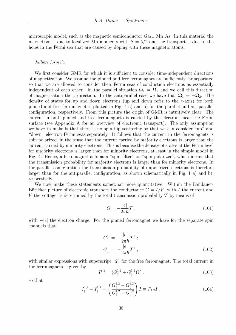
Julliere formula
We first consider GMR for which it is sufficient to consider time-independent directionsof magnetization. We assume the pinned and free ferromagnet are sufficiently far separatedso that we are allowed to consider their Fermi seas of conduction electrons as essentiallyindependent of each other. In the parallel situation Ω1 = Ω2 and we call this directionof magnetization the z-direction. In the antiparallel case we have that Ω1 = −Ω2. Thedensity of states for up and down electrons (up and down refer to the z-axis) for bothpinned and free ferromagnet is plotted in Fig. 4 a) and b) for the parallel and antiparallelconfiguration, respectively. From this picture the origin of GMR is intuitively clear. Thecurrent in both pinned and free ferromagnets is carried by the electrons near the Fermisurface (see Appendix A for an overview of electronic transport). The only assumptionwe have to make is that there is no spin flip scattering so that we can consider “up” and“down” electron Fermi seas separately. It follows that the current in the ferromagnets isspin polarized, in the sense that the current carried by majority electrons is larger than thecurrent carried by minority electrons. This is because the density of states at the Fermi levelfor majority electrons is larger than for minority electrons, at least in the simple model inFig. 4. Hence, a ferromagnet acts as a “spin filter” or “spin polarizer”, which means thatthe transmission probability for majority electrons is larger than for minority electrons. Inthe parallel configuration the transmission probability of unpolarized electrons is thereforelarger than for the antiparallel configuration, as shown schematically in Fig. 1 a) and b),respectively.
We now make these statements somewhat more quantitative. Within the Landauer-Butikker picture of electronic transport the conductance G = I/V , with I the current andV the voltage, is determined by the total transmission probability T by means of
G = − |e|2π~
T , (101)
with −|e| the electron charge. For the pinned ferromagnet we have for the separate spinchannels that
G1↑ = − |e|
2π~T 1↑ ;
G1↓ = − |e|
2π~T 1↓ , (102)
with similar expressions with superscript “2” for the free ferromagnet. The total current inthe ferromagnets is given by
I1,2 = (G1,2↑ + G1,2
↓ )V , (103)
so that
I1,2↑ − I1,2
↓ =
(G1,2↑ −G1,2
↓G1,2↑ + G1,2
↓
)I ≡ P1,2I , (104)
38
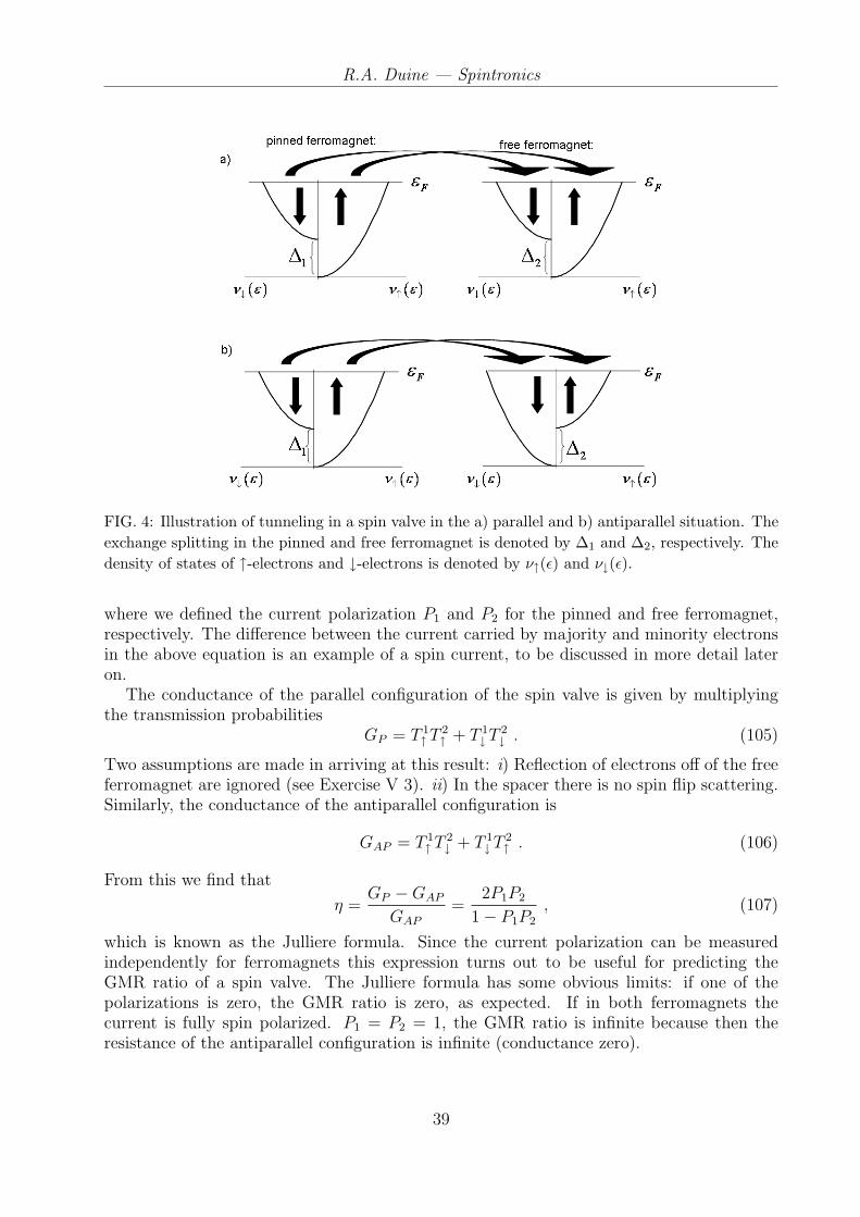
R.A. Duine — Spintronics
FIG. 4: Illustration of tunneling in a spin valve in the a) parallel and b) antiparallel situation. Theexchange splitting in the pinned and free ferromagnet is denoted by ∆1 and ∆2, respectively. Thedensity of states of ↑-electrons and ↓-electrons is denoted by ν↑(ε) and ν↓(ε).
where we defined the current polarization P1 and P2 for the pinned and free ferromagnet,respectively. The difference between the current carried by majority and minority electronsin the above equation is an example of a spin current, to be discussed in more detail lateron.
The conductance of the parallel configuration of the spin valve is given by multiplyingthe transmission probabilities
GP = T 1↑ T
2↑ + T 1
↓ T2↓ . (105)
Two assumptions are made in arriving at this result: i) Reflection of electrons off of the freeferromagnet are ignored (see Exercise V 3). ii) In the spacer there is no spin flip scattering.Similarly, the conductance of the antiparallel configuration is
GAP = T 1↑ T
2↓ + T 1
↓ T2↑ . (106)
From this we find that
η =GP −GAP
GAP
=2P1P2
1− P1P2
, (107)
which is known as the Julliere formula. Since the current polarization can be measuredindependently for ferromagnets this expression turns out to be useful for predicting theGMR ratio of a spin valve. The Julliere formula has some obvious limits: if one of thepolarizations is zero, the GMR ratio is zero, as expected. If in both ferromagnets thecurrent is fully spin polarized. P1 = P2 = 1, the GMR ratio is infinite because then theresistance of the antiparallel configuration is infinite (conductance zero).
39

R.A. Duine — Spintronics
FIG. 5: Illustration of spin transfer torques in spin valves.
Spin transfer from conservation of total spin angular momentum
We have seen that experimentally it is possible to alter the magnetic state of the spinvalve by driving a (large) current through it. Before going through the calculations we givesome simple physical arguments of the physics behind this. Consider the situation in Fig. 5:the pinned and free ferromagnet are misaligned. As explained, the pinned ferromagnet willpolarized the electrons, as they pass through it, in the direction of its magnetization. Inturn, the free ferromagnet will polarize the electrons in the direction of the magnetizationof the free ferromagnet. This implies that the free ferromagnet changes the direction ofmagnetization of the conduction electrons as they pass through it, i.e., the free ferromagnetexerts a torque on the conduction electron spins. Hence, appealing to conservation of angularmomentum, the conduction electrons exert an equal and opposite torque to the direction ofmagnetization of the free ferromagnet. This torque, which essentially comes from transferof angular momentum from the conduction electrons to the magnetization, is called the spintransfer torque, and denoted by ΓSTT in Fig. 5.
We now make these intuitive results more quantitative using the s−d model. We make theso-called adiabatic approximation. It consists of assuming that the time-scales associatedwith the change of magnetization direction Ω(x, t) are so slow that we can consider theelectrons as moving in a inhomogeneous time-independent Zeeman magnetic field in thedirection of the instantaneous magnetization. This approximation is based on the fact thatelectron time scales ~/εF ∼ 10−15 s, whereas the time scales for changes in magnetizationdirection are of the order of nanoseconds. The wave function ψκ
σ(x, t) of one electron withspin state |σ〉 in an orbital labelled by κ is then determined by the Schrodinger equation
i~∂ψκ
σ(x, t)
∂t=
[−~
2∇2
2m+ V (x)
]ψκ
σ(x, t)− ∆
2
∑
σ′Ω(x) · τσ,σ′ψ
κσ′(x, t) . (108)
40

R.A. Duine — Spintronics
We consider now the local change in spin angular momentum. Therefore, we need to calculate
∂sκ(x, t)
∂t≡ ~
2
∂
∂t
∑
σ,σ′(ψκ
σ)∗(x, t)τσ,σ′ψκσ′(x, t) . (109)
From Eq. (108) we find that
∂(sκ(x, t))α
∂t+∇ · (Jκ
s (x, t))α =∆
~sκ(x, t)×Ω(x)|α , (110)
where the spin current for orbital κ is defined as
(Jκs (x, t))α =
~2
4mi
∑
σ,σ′
[(ψκ
σ(x, t))∗τασ,σ′∇ψκ
σ′(x, t)− (∇ψκσ(x, t))∗τα
σ,σ′ψκσ′(x, t)
]. (111)
The left-hand side of Eq. (110) looks like a continuity equation for a conserved quantity. Theright-hand side, however, reveals the fact that spin is not conserved. It describes precessionof the electrons spins around the magnetization. For comparison, consider the continuityequation for the charge density Qκ ≡ −|e|∑σ(ψκ
σ)∗ψκσ, given by
∂Qκ(x, t)
∂t+∇ · Jκ
c (x, t) = 0 , (112)
with the charge current
Jκc (x, t) = − |e|~
2mi
∑σ
[(ψκσ(x, t))∗∇ψκ
σ(x, t)− (∇ψκσ(x, t))∗ψκ
σ(x, t)] . (113)
Note that because charge is a conserved quantity the right-hand side of Eq. (112) containsno source terms, and it is therefore a continuity equation. A few remarks are in order atthis point. We have defined the spin density and spin current in Eq. (110) such that thespin density has units of [angular momentum]/[volume], and therefore the spin current hasunits [angular momentum] × [density] × [velocity]. The charge current has units [charge] ×[density] × [velocity]. Note that we use the terms current and current density for the samephysical concept.
The total (spin) density and (spin) current are formally calculated by summing over alloccupied orbitals κ. Of course, the way in which the orbitals are occupied is in principle verycomplicated. In the situation that a current is carried through the system the distributionfunction that determines the orbital occupation is a nonequilibrium distribution function.We have, however, already seen that the current and spin current are in a ferromagnetrelated by a polarization factor as in Eq. (104). We assume, therefore, that in a ferromagnetwith direction of magnetization Ω which carries a total charge current Jc, the spin currentis given by
Jαs = −~PΩα
2|e| Jc . (114)
In Appendix A we sketch how to calculate P within two approximation schemes.We already hinted at the fact that the spin of the conduction electrons is not conserved
as the right-hand side of Eq. (110) describes precession the electron spin around the localmagnetization. The total spin angular momentum of conduction electrons and magnetization
41
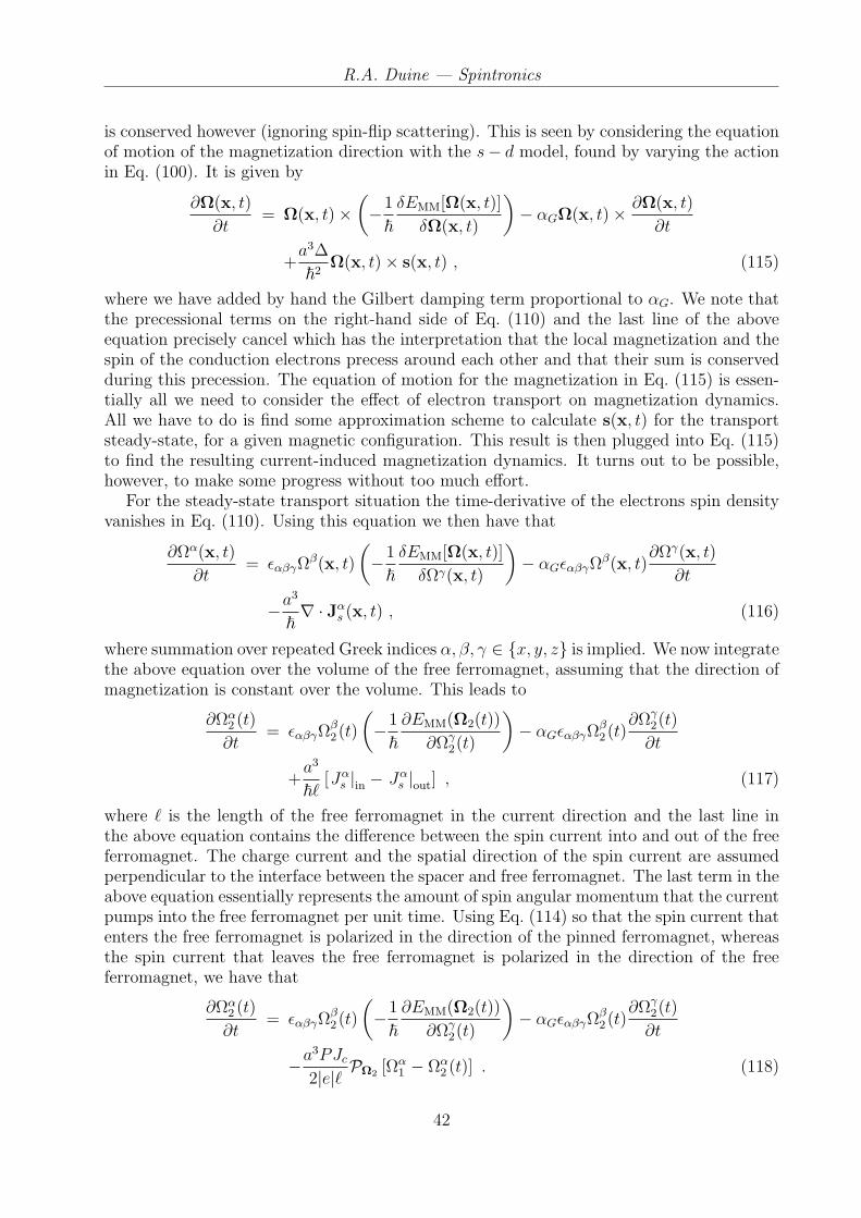
R.A. Duine — Spintronics
is conserved however (ignoring spin-flip scattering). This is seen by considering the equationof motion of the magnetization direction with the s− d model, found by varying the actionin Eq. (100). It is given by
∂Ω(x, t)
∂t= Ω(x, t)×
(−1
~δEMM[Ω(x, t)]
δΩ(x, t)
)− αGΩ(x, t)× ∂Ω(x, t)
∂t
+a3∆
~2Ω(x, t)× s(x, t) , (115)
where we have added by hand the Gilbert damping term proportional to αG. We note thatthe precessional terms on the right-hand side of Eq. (110) and the last line of the aboveequation precisely cancel which has the interpretation that the local magnetization and thespin of the conduction electrons precess around each other and that their sum is conservedduring this precession. The equation of motion for the magnetization in Eq. (115) is essen-tially all we need to consider the effect of electron transport on magnetization dynamics.All we have to do is find some approximation scheme to calculate s(x, t) for the transportsteady-state, for a given magnetic configuration. This result is then plugged into Eq. (115)to find the resulting current-induced magnetization dynamics. It turns out to be possible,however, to make some progress without too much effort.
For the steady-state transport situation the time-derivative of the electrons spin densityvanishes in Eq. (110). Using this equation we then have that
∂Ωα(x, t)
∂t= εαβγΩ
β(x, t)
(−1
~δEMM[Ω(x, t)]
δΩγ(x, t)
)− αGεαβγΩ
β(x, t)∂Ωγ(x, t)
∂t
−a3
~∇ · Jα
s (x, t) , (116)
where summation over repeated Greek indices α, β, γ ∈ x, y, z is implied. We now integratethe above equation over the volume of the free ferromagnet, assuming that the direction ofmagnetization is constant over the volume. This leads to
∂Ωα2 (t)
∂t= εαβγΩ
β2 (t)
(−1
~∂EMM(Ω2(t))
∂Ωγ2(t)
)− αGεαβγΩ
β2 (t)
∂Ωγ2(t)
∂t
+a3
~`[Jα
s |in − Jαs |out] , (117)
where ` is the length of the free ferromagnet in the current direction and the last line inthe above equation contains the difference between the spin current into and out of the freeferromagnet. The charge current and the spatial direction of the spin current are assumedperpendicular to the interface between the spacer and free ferromagnet. The last term in theabove equation essentially represents the amount of spin angular momentum that the currentpumps into the free ferromagnet per unit time. Using Eq. (114) so that the spin current thatenters the free ferromagnet is polarized in the direction of the pinned ferromagnet, whereasthe spin current that leaves the free ferromagnet is polarized in the direction of the freeferromagnet, we have that
∂Ωα2 (t)
∂t= εαβγΩ
β2 (t)
(−1
~∂EMM(Ω2(t))
∂Ωγ2(t)
)− αGεαβγΩ
β2 (t)
∂Ωγ2(t)
∂t
−a3PJc
2|e|` PΩ2 [Ωα1 − Ωα
2 (t)] . (118)
42

R.A. Duine — Spintronics
From Eq. (115) we see that that term proportional to current has to be perpendicular to themagnetization. Within the approximation of Eq. (114) this may be no longer true, which iswhy we have introduced the projection operation PΩ that projects out the part parallel toΩ. Carrying out this projection explicitly we have that
∂Ω2(t)
∂t= Ω2(t)×
(−1
~∂EMM(Ω2(t))
∂Ω2(t)
)− αGΩ2(t)× ∂Ω2(t)
∂t
−a3PJc
2|e|` Ω2(t)× [Ω1 ×Ω2(t)] . (119)
The last term in this equation is the spin transfer torque as first derived by Slonczewskiand is therefore sometimes also called the Slonczewksi torque. The form of this torque isquite special. This is seen qualitatively as follows. Consider the effective field Heff in thez-direction and Ω1 also in this direction. Then, depending on current, the damping and spintransfer torque can point in precisely opposite directions so that there will be magnetizationdynamics if αGHeff ∼ a3PJc/(|e|`) leading to a critical current
Jcritc ∼ αG|e|`Heff
a3P. (120)
This beneficial (in the sense of lowering the critical current) factor of αG ¿ 1 for current-induced dynamics that usually leads to switching of the free ferromagnet, as opposed to acritical switching field which will be Hcrit ∼ Heff , makes spin transfer torques an ideal basisfor building magnetic memory devices.
At first sight it may be a little suspicious that from Eq. (114) we are actually able toderive a torque on the free ferromagnet. After all, doesn’t Eq. (114) imply that the spin ofthe conduction electrons is parallel to the local magnetization so that there is no torque onthe local magnetization by the spin of the conduction electrons? The crucial thing is thatupon entering the free ferromagnet the spin of the conduction electrons is aligned with thepinned ferromagnet and therefore misaligned with the magnetization of the free ferromagnet.While passing through the free ferromagnet the spins of the conduction electrons align withthe free ferromagnet and the spin angular momentum of the conduction electrons is absorbedby the magnetization of the free ferromagnet.
To put this a little more quantitative consider one electron entering the free ferromagnet(whose direction of magnetization we chose the to be the z-direction) with the wave function
ψ(x, y) ∝ χk↑⊥(y)eik↑‖x| ↑〉+ ∝ χk↓⊥
(y)eik↓‖x| ↓〉 , (121)
where x is in the current direction and y in the direction transverse to current (we considerthe two-dimensional situation for simplicity). The wave function for the transverse modelabelled by k is indicated by χk(y). The wave numbers are constrained so that we areconsidering an electron at the Fermi level:
(kσ‖ )
2 + (kσ⊥)2 = k2
F +σ∆2
2≡ k2
Fσ . (122)
The conduction electron spin perpendicular to the direction of magnetization of the freeferromagnet is given by
sk⊥(x, y) ∝ sin
(√k2
F + ∆2/2− k2⊥x−
√k2
F −∆2/2− k2⊥x
)x
43

R.A. Duine — Spintronics
+ cos
(√k2
F + ∆2/2− k2⊥x−
√k2
F −∆2/2− k2⊥x
)y . (123)
Upon averaging over all transverse channels the total spin density
s(x, y) ∝∫
dk⊥sk⊥(x, y) , (124)
which can be shown to decay algebraically into the free ferromagnet, i.e., as a function of x.Although there is no typical length scale for this decay, beyond the so-called spin coherencelength
`sc ∼ 1
kF↑ − kF↓, (125)
the spins of the conduction electrons are practically aligned with the local magnetization.We conclude, therefore, that the spin transfer torque in a spin valve is a surface torque,i.e., the angular momentum transfer from the spin of the conduction electrons to the localmagnetization takes place near the surface separating the free ferromagnet and spacer.
Exercises
1. Spin current
Derive equations Eq. (110-113) from the Schrodinger equation [Eq. (108)].
2. Critical current and switching
Consider the following expression for the micromagnetic energy:
EMM(Ω2) = −Kz(Ωz2)
2
2.
Consider the situation with Ω1 = z and Ω2 = −z. Perform a linear stability analysis usingEq. (119) to determine as a function of current when Ω2 = −z is stable or unstable. Considerboth positive and negative current. Explain, using these results, the experimental result inFig. 3.
3. Composition rules for two scatterers
Consider two scatterers in one dimension (we ignore electron spin in this exercise). Thefirst scatterer has transmission amplitude t1 and reflection amplitude r1 for waves incomingfrom the left. For waves incoming from the right these amplitude are denoted by t′1 and r′1.Similar notation holds for scatterer two.
a) Show that the transmission amplitude of the two scatterers combined (scatterer 1 isplaced left of scatterer 2) is given by
t = t2(1− r′1r2)−1t1 .
44
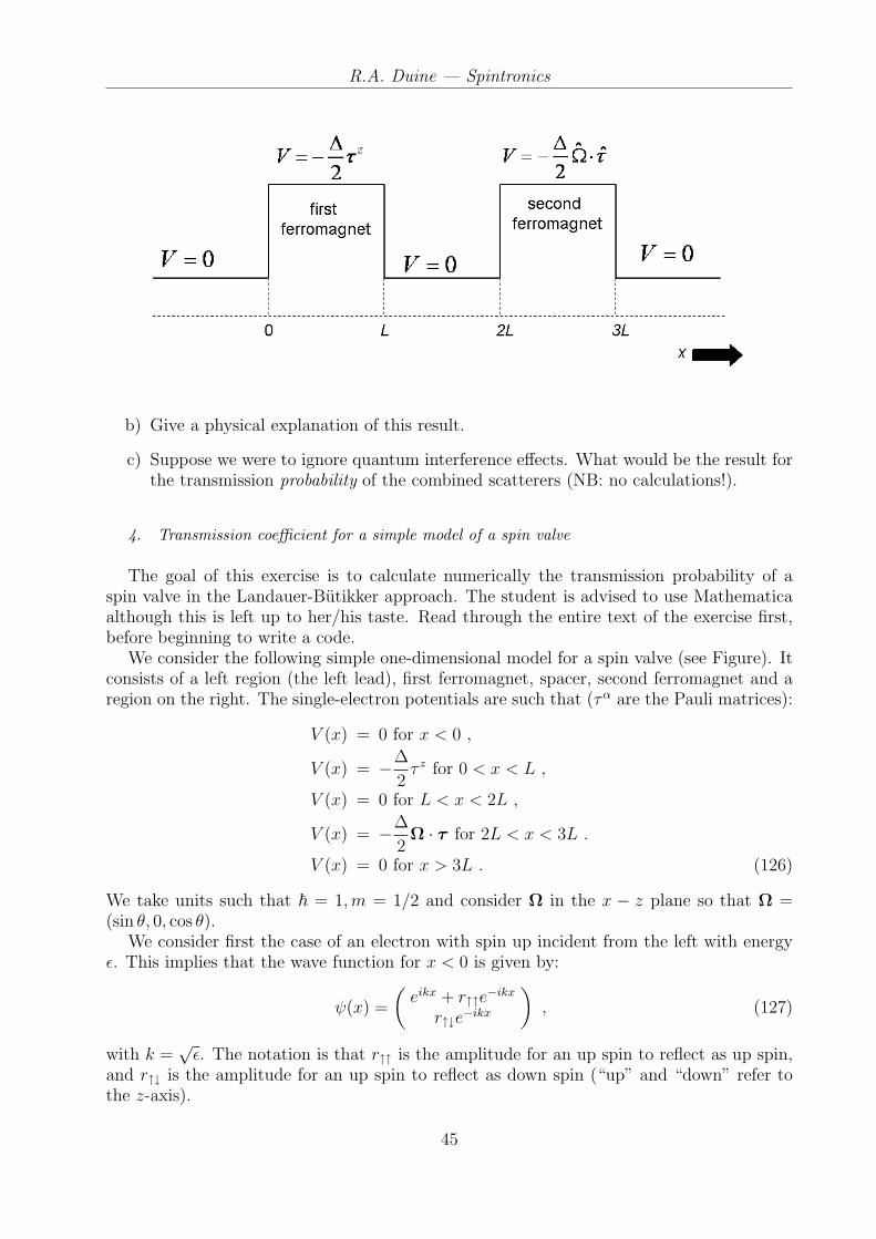
R.A. Duine — Spintronics
b) Give a physical explanation of this result.
c) Suppose we were to ignore quantum interference effects. What would be the result forthe transmission probability of the combined scatterers (NB: no calculations!).
4. Transmission coefficient for a simple model of a spin valve
The goal of this exercise is to calculate numerically the transmission probability of aspin valve in the Landauer-Butikker approach. The student is advised to use Mathematicaalthough this is left up to her/his taste. Read through the entire text of the exercise first,before beginning to write a code.
We consider the following simple one-dimensional model for a spin valve (see Figure). Itconsists of a left region (the left lead), first ferromagnet, spacer, second ferromagnet and aregion on the right. The single-electron potentials are such that (τα are the Pauli matrices):
V (x) = 0 for x < 0 ,
V (x) = −∆
2τ z for 0 < x < L ,
V (x) = 0 for L < x < 2L ,
V (x) = −∆
2Ω · τ for 2L < x < 3L .
V (x) = 0 for x > 3L . (126)
We take units such that ~ = 1,m = 1/2 and consider Ω in the x − z plane so that Ω =(sin θ, 0, cos θ).
We consider first the case of an electron with spin up incident from the left with energyε. This implies that the wave function for x < 0 is given by:
ψ(x) =
(eikx + r↑↑e−ikx
r↑↓e−ikx
), (127)
with k =√
ε. The notation is that r↑↑ is the amplitude for an up spin to reflect as up spin,and r↑↓ is the amplitude for an up spin to reflect as down spin (“up” and “down” refer tothe z-axis).
45

R.A. Duine — Spintronics
a) Show that the wave function in the spacer is of the form:
ψ(x) =
(Aeikx + Be−ikx
Ceikx + De−ikx
). (128)
b) Give also the wave functions in the first ferromagnet and the region x > 3L.
c) The wave function in the second ferromagnet is of the form:
ψ(x) =[Aeik(∆)x + Be−ik(∆)x
]χ+(θ) +
[Ceik(−∆)x + De−ik(−∆)x
]χ−(θ) , (129)
where χ±(θ) are spinors such that
Ω · τχ±(θ) = ±χ±(θ) ,
and
k(∆) =
√ε +
∆
2.
Give the expressions for χ+(θ) and χ−(θ) in terms of
| ↑〉 =
(10
);
| ↓〉 =
(01
). (130)
Note that we need this result for the wave function matching later on.
d) To solve the Schrodinger equation we require that the wave function and its firstderivative are continuous at the boundaries between the various regions. Give theresulting equations. Count the number of equations and number of unknowns (answer:both should be 16).
e) Write a program that solves these equation numerically for given θ. Use ∆ = 6, L = 1,and ε = 1.
(hint: in mathematica the function “Solve” will do the trick).
f) To check your numerical results plot |t↑↑(θ)|2 + |t↑↓(θ)|2 + |r↑↑(θ)|2 + |r↑↓(θ)|2 as afunction of θ ∈ [0, π] (tσσ′ is the amplitude for an incident electron with spin |σ〉 totransmit with spin |σ′〉). What should the result for this quantity be?
g) Same as part e), but consider now the case that an electron with spin down is incidentfrom the left. Note that you only have modify your numerical code slightly for thispart of the exercise.
When you hand in this exercise provide a print-out (NB: hand in as hardcopy, notelectronic) of your code together with (or including) print-outs of plots of:
1. The reflections probabilities |rσσ′(θ)|2 for an incident electron with spin |σ〉 toreflect with spin |σ′〉, for all values of σ and σ′, as a function of θ ∈ [0, π]. (4plots)
46

R.A. Duine — Spintronics
2. The transmission probabilities |tσσ′(θ)|2 for an incident electron with spin |σ〉 totransmit with spin |σ′〉, for all values of σ and σ′, as a function of θ ∈ [0, π]. (4plots)
3. The transmission probability for an unpolarized current T (θ) =∑
σσ′ |tσσ′(θ)|2 asa function of θ ∈ [0, π]. (1 plot)
Additional reading
Slonczewski’s original paper on spin transfer:
• J.C. Slonczewski, J. Mag. Mat. Mag. 159, L1 (1996).
Berger’s original paper on spin transfer:
• L. Berger, Phys. Rev. B 54, 9353 (1996).
The first experimental observations:
• M. Tsoi , A. G. M. Jansen, J. Bass, W.-C. Chiang, M. Seck, V. Tsoi, and P. Wyder,Phys. Rev. Lett. 80, 4281 (1998).
• E. B. Myers, D. C. Ralph, J. A. Katine, R. N. Louie, R. A. Buhrman, Science 285,867 (1999).
47

R.A. Duine — Spintronics
VI. SPIN TRANSFER TORQUES FOR SMOOTH MAGNETIZATION TEX-TURES
In the previous section we have seen that spin transfer torques occur when an electrictransport current flows through a noncollinear magnetic material (noncollinear means thatthe magnetization is pointing in different directions at different positions). In this sectionwe will look at spin transfer torques in the limit that the magnetization direction variessmoothly and slowly so that we are allowed to perform a long-wavelength small-frequencyapproximation similar like the calculations done in Exercise III 8. This so-called gradientexpansion is most elegantly set up in terms of fictitious gauge fields. Therefore, we startthis section by reviewing gauge theory and its connection to conservation laws.
Before discussing these concepts in more detail we briefly state some notational def-initions. In this section we will in the notation suppress the sum over spin indicesσ, σ′, . . . ∈ ↑, ↓. This is done easiest by introducing the spinor
φ ≡(
φ↑φ↓
), (131)
with its complex transpose is denoted by
φ† ≡ (φ∗↑, φ
∗↓)
. (132)
Using this notation, terms that involve the Pauli matrices are written as matrix products,e.g., ∑
σ,σ′φ∗στ
µσ,σ′φσ′ = φ†τµφ . (133)
In this way we also write terms diagonal in spin space as matrix products, e.g.,∑
σ
φ∗σφσ = φ†φ . (134)
Symmetries, conservation laws, and gauge fields
Global symmetries of physical systems are related to conservation laws via Noether’stheorem. For example, translational and rotational invariance gives rise to conservation oflinear and angular momentum, respectively. Attempts to make these global symmetrieslocal come at the cost of introducing additional fields: gauge fields. For example, the gaugefield associated with particle number conservation, i.e., the gauge field one has to introducewhen elevating the global symmetry associated with particle-number conservation to a localsymmetry, is the electromagnetic field.
Charge conservation: global U(1) symmetry
We consider a general action for fermions (electrons) which is the sum of a single-particlepiece containing the kinetic energy, and other terms, like interactions,
AE[φ†,φ] =
∫ ~βT
0
dτ
∫dxφ†(x, τ)
(~
∂
∂τ− ~
2∇2
2m
)φ(x, τ) + H
[φ†,φ
]
. (135)
48

R.A. Duine — Spintronics
Here, H[φ†,φ
]is the hamiltonian functional that contains all contributions except kinetic
energy.The number of electrons is conserved. This implies that in the action only terms with
an equal number of φ† and φ fields appear since in the operator langauge this correspondsto an equal number of creation and annihilation operators. Mathematically particle num-ber conservation results in invariance of the action under multiplication of the field by anarbitrary phase factor, i.e., the action in Eq. (135) is invariant if we transform the fieldsaccording to
φ(x, τ) → φ(x, τ)eiΛ ;
φ†(x, τ) → φ†(x, τ)e−iΛ , (136)
with Λ independent of x and τ . Since the phase factors eiΛ form a representation of thegroup U(1), this symmetry is called global U(1) symmetry.
Because of the space and time derivatives the action is not invariant under local U(1)transformations, i.e., changes of the fields according to Eq. (136) with Λ dependent on spaceand imaginary time. The variation δAE of the action under infinitesimal versions of suchlocal transformations is defined by
AE
[φ†,φ
]+ δAE +O [Λ]2 = AE
[φ†(1− iΛ),φ(1 + iΛ)
], (137)
and reads
δAE =
∫ ~βT
0
dτ
∫dxΛ(x, τ)
−i~
∂
∂τ
(φ†(x, τ)φ(x, τ)
)
− ~2
2mi∇ · [φ†(x, τ)∇φ(x, τ)− (∇φ†(x, τ)
)φ(x, τ)
]. (138)
Since putting general variations of the action equal to zero gives the equations of motion,and because the local phase variation is just a specific case of a variation, we have that
i∂
∂τ
⟨φ†(x, τ)φ(x, τ)
⟩+
~2mi
⟨∇ · [φ†(x, τ)∇φ(x, τ)− (∇φ†(x, τ))φ(x, τ)
]⟩= 0 . (139)
Note that after multiplying the above equation with the electronic charge −|e| and substitut-ing τ → it we recover Eq. (112), which reveals the connection between charge conservationand U(1) symmetry.
U(1) gauge theory
If we try to elevate the global U(1) symmetry of the action in Eq. (135) to a local one, weend up with a U(1) gauge theory. To see this note that if we transform the fields accordingto
φ(x, τ) → φ(x, τ)eiΛ(x,τ) ;
φ†(x, τ) → φ†(x, τ)e−iΛ(x,τ) , (140)
49

R.A. Duine — Spintronics
the action gets additional terms
AE[φ†,φ] =
∫ ~βT
0
dτ
∫dx
[φ†(x, τ)
(~
∂
∂τ+ i~
∂Λ(x, τ)
∂τ
)φ(x, τ)− φ†(x, τ)
~2∇2
2mφ(x, τ)
− ~2
2mφ†(x, τ)
[2i(∇Λ(x, τ)) · ∇φ(x, τ) +∇2φ(x, τ)− φ(x, τ)∇2Λ(x, τ)
] ]+ H
[φ†,φ
] .
(141)
The additional terms that involve Λ(x, τ) are transformed away by introducing gauge fieldsa(x, τ) and a0(x, τ). That is, the action
AE[φ†, φ, a, a0] =
∫ ~βT
0
dτ
∫dxφ†(x, τ)
(~
∂
∂τ+ ~a0(x, τ)− ~
2(∇+ a(x, τ))2
2m
)φ(x, τ)
+H[φ†,φ
] , (142)
is invariant under the local U(1) transformation in Eq. (140) provided we let the gauge fieldstransform simultaneously according to
a0(x, τ) → a0(x, τ)− i∂Λ(x, τ)
∂τ;
a(x, τ) → a(x, τ)− i∇Λ(x, τ) . (143)
The way the gauge fields couple to the charge fields (with charge fields we mean the φ† andφ) is by replacing
∂
∂τ→ ∂
∂τ+ a0(x, τ) ;
∇ → ∇+ a(x, τ) . (144)
This way of coupling gauge fields to matter fields is called minimal coupling.So far, this is all a mathematical exercise. Experimentally we know, however, that there
do exist gauge fields that couple to charge according to the action in Eq. (142): the vectorand scalar potential of electromagnetism! These are denoted by Aem(x, τ) and Vem(x, τ),respectively, and give the magnetic field B = ∇ × Aem and electric field E = −∇Vem −i∂A/(c∂τ). After substitution of a0 = −|e|Vem/~ and a = −|e|Aem/(i~c), with c thevelocity of light, we have the familiar action
AE[φ†,φ,Aem, Vem] =∫ ~βT
0
dτ
∫dxφ†(x, τ)
(~
∂
∂τ− |e|Vem(x, τ) +
1
2m
(−i~∇+
|e|c
Aem(x, τ)
)2)
φ(x, τ)
+H[φ†, φ
]
,
(145)
for electrons in the presence of magnetic and electric fields.
50

R.A. Duine — Spintronics
In the presence of a vector potential the definition of the current gets an additionalcontribution. To see this we consider the variation of the action under the transformationin Eq. (143). It is given by
δAE =
∫ ~βT
0
dτ
∫dxΛ(x, τ)
i~
∂
∂τ
(φ†(x, τ)φ(x, τ)
)
+~2
2mi∇ · [φ†(x, τ)∇φ(x, τ)− (∇φ†(x, τ)
)φ(x, τ)
]+|e|~c
Aem(x, τ)φ†(x, τ)φ(x, τ)
.
(146)
Because of gauge invariance we have δAE = 0. Therefore we have that
i∂
∂τ
⟨−|e|φ†(x, τ)φ(x, τ)⟩
+ 〈∇ · Jc(x, τ)〉 = 0 , (147)
with the charge current given by
Jc(x, τ) = − |e|~2mi
[φ†(x, τ)∇φ(x, τ)− (∇φ†(x, τ)
)φ(x, τ)
]− |e|2mc
Aem(x, τ)φ†(x, τ)φ(x, τ) .
(148)The last term on the right-hand side of this equation is called the diamagnetic contributionto the current. Without this term the current would not be gauge invariant.
SU(2): spin and spin currents revisited
We consider now an action for electrons coupled to an exchange magnetic field withdirection Ω(x, τ) given by
AE[φ†,φ,Ω] =
∫ ~βT
0
dτ
∫dxφ†(x, τ)
(~
∂
∂τ− ~
2∇2
2m
)φ(x, τ)
−∫
dx∆
2φ†(x, τ)Ω(x, τ) · τφ(x, τ) + H
[φ†,φ
]
, (149)
and show that we recover the definition of spin current in Eq. (111) by a local infinitesimalSU(2) transformation, essentially following the same steps at arriving at Eq. (139).
A general local SU(2) transformation is given by
φ(x, τ) → eiΛµ(x,τ)τµ
φ(x, τ) ;
φ†(x, τ) → φ†(x, τ)e−iΛµ(x,τ)τµ
, (150)
where a summation over µ ∈ x, y, z is implied. We assume that the hamiltonian is invariantunder this transformation, i.e.,
H[φ†, φ
]= H
[φ†(x, τ)e−iΛµ(x,τ)τµ
, eiΛµ(x,τ)τµ
φ(x, τ)]
. (151)
51

R.A. Duine — Spintronics
The variation of the action under an infinitesimal version of this transformation is then givenby
δAE =
∫ ~βT
0
dτ
∫dxΛµ(x, τ)
−i~
∂
∂τ
(φ†(x, τ)τµφ(x, τ)
)
− ~2
2mi∇ · [φ†(x, τ)τµ∇φ(x, τ)− (∇φ†(x, τ)
)τµφ(x, τ)
]
+∆εαµνΩα(x, τ)φ†(x, τ)τ νφ(x, τ)
. (152)
Putting this equal to zero yields
i∂
∂τ
⟨φ†(x, τ)τµφ(x, τ)
⟩+
~2mi
⟨∇ · [φ†(x, τ)τµ∇φ(x, τ)− (∇φ†(x, τ))τµφ(x, τ)
]⟩
=∆
2~εαµνΩα(x, τ)φ†(x, τ)τ νφ(x, τ) , (153)
in agreement with Eq. (111). Note that the source term on the right-hand side of thisequation comes from the fact that the term in the action that involves the exchange fielddoes not commute with the transformation in Eq. (150).
Spin transfer torques as gauge fields
To consider the effect of an electric transport current on the magnetization dynamics forbulk magnets we use the Stoner model discussed in Sec. III. We consider temperatures farbelow the critical temperature so that the magnetization direction is the relevant degree offreedom. The action is given by
AE[φ†,φ,Ω] =
∫ ~βT
0
dτ
∫dx
φ†(x, τ)
(~
∂
∂τ− ~
2∇2
2m− µ
)φ(x, τ)
−∆
2φ†(x, τ)Ω(x, τ) · τφ(x, τ)− gBφ†(x, τ)τ zφ(x, τ)
, (154)
where we included an external Zeeman magnetic field in the z-direction. We now transformthe spinors according to the SU(2) transformation
φ(x, τ) = R(Ω(x, τ))φ′(x, τ) , (155)
with the SU(2) rotation matrix in spin space determined from
R−1(Ω)Ω · τR(Ω) = τ z . (156)
Physically, the new fermion fields φ′ correspond to electrons which have their spin quanti-zation axis parallel to the local direction of magnetization.
After this transformation the action is given by
AE[(φ′)†, φ′,Ω] =
∫ ~βT
0
dτ
∫dx
(φ′)†
(~
∂
∂τ+ ~a0 − ~
2∇2
2m− ∆
2τ z − µ
)φ′
+~2
2m
[∇(φ′)† · aφ′ − (φ′)† · a∇φ′ − (φ′)†a · aφ′]− gB(φ′)†Ω · τφ′
, (157)
52

R.A. Duine — Spintronics
with the gauge fields
a0(x, τ) ≡ R−1(Ω(x, τ))∂
∂τR(Ω(x, τ)) ;
a(x, τ) ≡ R−1(Ω(x, τ))∇R(Ω(x, τ)) . (158)
This action is very similar to the action in Eq. (142). The difference, however, is that theabove gauge fields are SU(2) gauge fields, i.e., they are SU(2) matrix valued. We denotethe spatial components of a with aα. Note that for each α, aα takes values in SU(2). Hence,we have that
a0(x, τ) = aµ0(x, τ)τµ ;
aα(x, τ) = aµα(x, τ)τµ . (159)
Note that we use subscript α, β, γ ∈ x, y, z for spatial indices, and superscript µ, ν ∈x, y, z for SU(2) indices.
The definition of the matrix R is ambiguous because we can still rotate the fermion fieldsaround the z-axis. Mathematically, this means that in Eq. (155) we can transform
φ′(x, τ) → eiΛ(x,τ)τz
φ′(x, τ) ;
R(Ω(x, τ)) → R(Ω(x, τ))e−iΛ(x,τ)τz
. (160)
This degree of freedom becomes a gauge degree of freedom for the action in Eq. (157). Thatis, the action in Eq. (157) is invariant — except for the term that involves the magnetic fieldB — under
φ′(x, τ) → eiΛ(x,τ)τz
φ′(x, τ ;
a0(x, τ) → a0(x, τ)− i∂Λ(x, τ)
∂ττ z ;
a(x, τ) → a(x, τ)− i∇Λ(x, τ)τ z , (161)
which is effectively a U(1) gauge degree of freedom since the above gauge transformationinvolves only τ z.
The measure of the path integral is unchanged under the transformation in Eq. (155) andwe can relabel φ′ → φ, which we will do from now on. The action in Eq. (157) is rewrittenas
AE[φ†,φ,Ω] =
∫ ~βT
0
dτ
∫dx
φ†(x, τ)
(~
∂
∂τ− ~
2∇2
2m− ∆
2τ z − µ
)φ(x, τ)
+~φ†(x, τ)τµφ(x, τ)aµ0(x, τ)− 2iJµ
s,α(x, τ)aµα(x, τ)
− ~2
2maµ
α(x, τ)aνα(x, τ)φ†(x, τ)τµτ νφ(x, τ)− gBφ†(x, τ)Ωαταφ(x, τ)
≡ A0E[φ†,φ] +Aint
E [φ†,φ,Ω] . (162)
To induce an electric transport current we now also couple the electrons to an externalelectromagnetic field via the minimal coupling in Eq. (144). The spin current in the above
53

R.A. Duine — Spintronics
equation is then defined by
Jµs,α(x, τ) =
~2
4mi
[φ†(x, τ)τµ∇αφ(x, τ)− (∇αφ†(x, τ)
)τµφ(x, τ)
]
+|e|~2mc
Aem,αφ†(x, τ)τµφ(x, τ) , (163)
in agreement with the gauge-invariant generalization of Eq. (111). The action A0E is defined
as
A0E[φ†,φ] =
∫ ~βT
0
dτ
∫dx
φ†(x, τ)
(~
∂
∂τ− |e|Vem(x, τ) +
1
2m
(−i~∇+
|e|c
Aem(x, τ)
)2
− ∆
2τ z − µ + Vdis(x)
)φ(x, τ)
, (164)
where we also included a spin-independent disorder potential Vdis(x) to make the electriccurrent finite. The remaining part of the action in Eq. (162) describes the coupling of theelectronic quasi-particles to the direction of magnetization Ω(x, τ) and is given by
AintE [φ†,φ,Ω] =
∫ ~βT
0
dτ
∫dx
~φ†(x, τ)τµφ(x, τ)aµ
0(x, τ)− 2iJµs,α(x, τ)aµ
α(x, τ)
− ~2
2maµ
α(x, τ)aµα(x, τ)φ†(x, τ)φ(x, τ)− gBφ†(x, τ)Ωα(x, τ)ταφ(x, τ)
. (165)
So far this seems only a mathematical exercise. We have, however, achieved the startingpoint for a systematic perturbation theory in the derivatives of Ω(x, τ), i.e., a gradientexpansion. To see this, we note that the gauge fields are in fact proportional to derivativesof Ω(x, τ), and define
a0(x, τ) ≡ R−1(Ω(x, τ))∂
∂τR(Ω(x, τ)) = Aα(Ω)
∂Ωα(x, τ)
∂τ;
a(x, τ) ≡ R−1(Ω(x, τ))∇R(Ω(x, τ)) = Aα(Ω)∇Ωα(x, τ) = Aα(Ω)∂Ωα(x, τ)
∂τ, (166)
withA(Ω) ≡ R−1(Ω)∇ΩR(Ω) . (167)
The effective action AeffE [Ω] for Ω(x, τ) is now defined via
Z =
∫d[φ†]d[φ]d[Ω]e−A0
E [φ†,φ]/~−AintE [φ†,φ,Ω]/~
=
∫d[φ†]d[φ]d[Ω]e−A0
E [φ†,φ]/~ (1− Aint
E [φ†,φ,Ω]/~+ · · ·)
=
∫d[Ω]Z0
(1− ⟨
AintE [φ†, φ,Ω]/~
⟩0+ 〈· · ·〉0
)
≡∫
d[Ω]e−AeffE [Ω]/~ . (168)
54
R.A. Duine — Spintronics
The · · · denote higher-order terms in the above Taylor expansion of the exponential, andthe average 〈· · ·〉0 is the expectation value with respect to the action in Eq. (164). For ourpurposes it is sufficient to keep only the first-order terms in the gradient expansion andthe magnetic field. The second-order terms contain information on the spin stiffness and inretaining them we would recover the results from Exercise III 8. The effective action thenbecomes
AeffE [Ω] =
∫ ~βT
0
dτ
∫dx
~ (n↑ − n↓) Az
α(Ω(x, τ))∂Ωα(x, τ)
∂τ
−2i〈Jzs,α(x, τ)〉0Az
β(Ω(x, τ))∇αΩβ(x, τ)− g (n↑ − n↓)B ·Ω(x, τ)
. (169)
Here we used that 〈φ†τµφ〉0 = (n↑−n↓)δµ,z in terms of the densities of majority and minorityelectrons, and that the spin current for the system described by Eq. (164) has spin directionz.
Finally, we need to determine the gauge field Azα(Ω). For this, it is easiest to write the
SU(2) rotation matrix asR(Ω) = mµ(Ω)τµ , (170)
with mµ a unit vector which obeys mµmµ = 1, so that we find from Eq. (167) that
Aν′α (Ω) = iεµνν′mµ(Ω)
∂mν(Ω)
∂Ωα
. (171)
It follows that
Azα(Ω) = i
[mx(Ω)
∂my(Ω)
∂Ωα
−my(Ω)∂mx(Ω)
∂Ωα
]. (172)
In polar coordinates Ω = (sin θ cos φ, sin θ sin φ, cos θ) we have explicitly that
m(θ, φ) = (sin(θ/2) cos φ, sin(θ/2) sin φ, cos(θ/2)) , (173)
which results in
Azr(θ, φ) = 0 ;
Azθ(θ, φ) = 0 ;
Azφ(θ, φ) =
i
2(1− cos θ) . (174)
The result for the effective action now becomes
AeffE [Ω] =
∫ ~βT
0
dτ
∫dx
i~2
(n↑ − n↓) [1− cos(θ(x, τ))]∂φ(x, τ)
∂τ
−~2
PJc,α
|e| [1− cos(θ(x, τ))]∇αφ(x, τ)− g (n↑ − n↓)B ·Ω(x, τ)
, (175)
where we used the relation in Eq. (114) between spin current and charge current in a collinearferromagnet. We assume that the charge current Jc is given and do not calculate it explicitlyis terms of the electric field. See, however, Appendix A.
55
R.A. Duine — Spintronics
Note that Eq. (174) implies that Az is related to the vector potential of a monopole!Using the results from Sec. II we rewrite the action as
AeffE [Ω] =
∫ ~βT
0
dτ
∫dx
i~2
(n↑ − n↓) Aβ(Ω(x, τ))∂Ωβ(x, τ)
∂τ
−~2
PJc,α
|e| Aβ(Ω(x, τ))∇αΩβ(x, τ)− g (n↑ − n↓)B ·Ω(x, τ)
, (176)
where the familiar monopole vector potential A(Ω) is determined from Eq. (25). This termis therefore understood as the spin Berry phase picked by the electron as it drifts throughthe magnetization texture with its spin following this texture adiabatically.
Variation of the above action gives, after going to real time via τ = it, the equation ofmotion for the magnetization direction
∂Ω(x, t)
∂t− P
|e|(n↑ − n↓)(Jc · ∇)Ω(x, t) =
2g
~Ω(x, t)×B . (177)
In this final result, the term that involves the electric current is known as the adiabatic spintransfer torque. In the next section we will see that the adiabatic spin transfer torque leadsto magnetization dynamics, and, in particular, to current-driven domain wall motion.
Exercises
1. Equation of motion
Derive Eq. (177) by variation of the action in Eq. (176). Use your results from the firstexercise of Sec. II.
2. Adiabatic spin transfer torque as a Slonczewski spin transfer torque
In the previous section we have seen that in a spin valve that consists of two ferromagnetswith direction Ω1 and Ω2, respectively, the current-induced torque on Ω2 is given by
∂Ω2(t)
∂t= −a3PJc
2|e|` Ω2(t)× [Ω1 ×Ω2(t)] . (178)
We model a bulk ferromagnet as a series of spin valves, and divide the system along thecurrent direction x in volume elements separate by a infinitesimal difference dx. Hence, weput Ω1 = Ω(x− dx), and Ω2(x).
a) Use Eq. (178) and show that you recover the adiabatic spin transfer torque in Eq. (177).
If spin is not completely conserved it turns out there exists also a spin torque of the form
∂Ω2(t)
∂t= −β
a3PJc
2|e|` [Ω1 ×Ω2(t)] , (179)
with β a dimensionless parameter.
b) Determine the additional torque that one now gets in the continuum (bulk) situation.This torque is known as the dissipative adiabatic spin transfer torque, sometimesreferred as non-adiabatic spin transfer torque, or simply “β-term”.
56

R.A. Duine — Spintronics
Additional reading
More on gauge fields:
• H. Kleinert, Gauge fields in condensed matter, World Scientific.
First derivation of the adiabatic spin transfer torque:
• Ya. B. Bazaliy, B.A. Jones, and Shou-Cheng Zhang, Phys. Rev. B 57, R3213 (1998).
57
R.A. Duine — Spintronics
VII. DOMAIN WALL MOTION
In this section 5 we consider the physics of magnetic domain walls, and, in particular,how an external magnetic field and electric current influence the domain-wall position. Wefirst consider static domain walls. Hereafter, field-driven and current-driven domain wallmotion are discussed.
Domain walls
We consider first the situation without external magnetic field or electric transport cur-rent. The energy functional with which we model the system is given in Eq. (95). In polarcoordinates θ and φ, defined by Ω = (sin θ cos φ, sin θ sin φ, cos θ), it is given by
E[θ, φ] =
∫dx
a3
Js
2
[(∇θ)2 + sin2 θ (∇φ)2] +
K⊥2
sin2 θ sin2 φ− Kz
2cos2 θ
. (180)
Recall that the above energy functional models a magnetic wire with length L À Ly, Lz.Here Ly and Lz are the length of the wire in the y and z-direction, respectively. (L is thelength in the x-direction.) The anisotropy constants K⊥, Kz > 0 and the exchange stiffnessJs > 0.
The lowest-energy states of the magnetization are homogeneous configurations such thatθ(x) = 0 or θ(x) = π, corresponding to magnetization parallel or antiparallel to the z-axis,respectively. In this model, domain walls are configurations that interpolate between suchconfigurations, i.e., magnetization configurations where the magnetization changes smoothlyfrom parallel to antiparallel to the z-axis in going along the x-direction (see Fig. 6). Themagnetization direction of these configurations does not depend on the transverse direction,however. Moreover, the magnetization lies in the x−z plane. Therefore, we look for solutionof the form θ(x) = θ(x) and φ(x) = 0, π. Varying the energy functional with respect to θgives
d2θ(x)
dx2= −Kz
Js
∂V (θ(x))
∂θ, (181)
which is the equation of motion for a particle with unit mass in a periodic potential
V (θ) =Kz
2Js
cos2 θ , (182)
with θ playing the role of the position of the particle and x being the time coordinate.Domain walls correspond to solutions where the particle starts out at “time” x = −∞ atone maximum of the potential, and ends up at another maximum at “time” x = +∞.To find these solutions we multiply Eq. (181) with dθ(x)/dx and integrate the equation ofmotion. The result is (
dθ(x)
dx
)2
+Kz
Js
cos2 θ(x) = C , (183)
with C an integration constant. Note that this equation essentially expresses energy conser-vation of the fictitious particle. The integration constant is fixed by noting that dθ/dx → 0and θ(x) → 0, π for x → ±∞, as required by having a domain wall. This implies C = Kz/Js.
5 This section was written with the help of Ties Lucassen.
58

R.A. Duine — Spintronics
wd
Lx
Ly
r (t)
L
xλ
z
y
FIG. 6: Illustration of a domain wall.
With this latter result the differential equation for θ(x) reads
(dθ(x)
dx
)2
=Kz
Js
sin2 θ(x) . (184)
Since θ ∈ [0, π) we can safely take the square-root of this equation. Hence we have that
dθ
dx= ±
√Kz
Js
sin θ(x) ⇒ dθ
sin θ= ±
√Kz
Js
dx . (185)
We integrate this equation from the position of the domain wall rdw, where θ(rdw) = π/2,to arbitrary x. Thus we find
∫ θ(x)
π/2
dθ
sin θ= ±
√Kz
Js
(x− rdw) ⇒ log
[tan
(θ
2
)]= ±
√Kz
Js
(x− rdw) . (186)
Inverting the latter result gives the domain-wall solution for a domain at position rdw:
θ(x) = 2 tan−1[eQ(x−rdw)/λ
]. (187)
In this expression the length scale
λ =
√Js
Kz
, (188)
is called the domain-wall width. The so-called charge Q = ±1 determines whether themagnetization changes from +z to −z (Q = 1) or opposite (Q = −1). The domain-wall width is the length scale over which the magnetization changes direction. For eachof the two possible charges the angle φ = 0 or π determines in which sense (clockwiseor counterclockwise) the magnetization changes direction. Hence, this angle determines theso-called chirality of the domain wall. In the next section we consider domain-wall dynamics.
Moving domain walls
To consider the possible motion of a domain wall due to electric currents and/or externalfields we have to solve the equation of motion for the direction of magnetization. Using theresult from Eq. (177) it is in first instance given by
(∂
∂t+ vs · ∇
)Ω(x, t) = Ω(x, t)×
(−1
~δE[Ω]
δΩ(x, t)+
gB
~
)− αGΩ(x, t)× ∂Ω(x, t)
∂t, (189)
59

R.A. Duine — Spintronics
with B the external field and αG the Gilbert damping constant. The velocity vs is definedas
vs = −a3PJc
|e| . (190)
The physical meaning of this velocity is elucidated as follows. Consider Eq. (189) with B = 0and αG = 0. Suppose Ω0(x) is a time-independent solution for vs = 0, for example a domain-wall magnetization texture. Then Ω0(x − vst) is a time-dependent solution with vs 6= 0,corresponding to “drift” of the magnetization texture with the velocity vs determined bythe current. In the case of a domain wall, the domain wall position will therefore simplymove with the velocity vs in the absence of Gilbert damping and/or an external magneticfield.
The above argument has caused some motivation to alter the Gilbert damping termaccordingly, i.e., to make the replacement
∂
∂t→ ∂
∂t+ v · ∇ , (191)
on the right-hand side of Eq. (189). This turns out, however, to be not completely correct.The electric current does nonetheless change the Gilbert damping term. It turns out thatthe full equation of motion for the magnetization direction in the presence of current is givenby
(∂
∂t+ vs · ∇
)Ω(x, t) = Ω(x, t)×
(−1
~δE[Ω]
δΩ(x, t)+
gB
~
)
−αGΩ(x, t)×(
∂
∂t+
β
αG
vs · ∇)
Ω(x, t) , (192)
where the dimensionless β-parameter characterizes the so-called dissipative spin transfertorque (see Exercise VI 2).
To get the physics out of this equation we are going to solve it variationally. To bespecific, our trial solution is a domain wall solution corresponding to a domain wall in whichthe magnetization direction changes from the −z to +z direction. It is given by
θ(x, t) = θ0(x, t) ≡ 2 tan−1[e−(rdw(t)−x)/λ
];
φ(x, t) = φ0(t) . (193)
The two variational parameters in this ansatz are the domain-wall position rdw(t) and theangle φ0(t) that determines the domain-wall chirality. It turns out that these two variationalparameters are canonically conjugate to each other. Note that in principle we could addadditional variational parameters, such as the domain-wall width. The description we usehere turns out to already take into account a great deal of the physics qualitatively.
In order to find the equation of motion for the domain-wall position and the domain-wallchirality we need an appropriate variational principle. The equation of motion in Eq. (192)without damping terms, i.e., with β = αG = 0, is found by varying the real-time action
A[θ, φ] =
∫dt
[∫dx
a3~ (cos θ(x, t)− 1)
(∂
∂t+ vs
∂
∂x
)φ(x, t)− gB cos θ(x, t)
]− E[θ, φ]
.
(194)
60
R.A. Duine — Spintronics
Note that we have chosen the current in the x-direction and the external magnetic fieldin the −z direction (with this choice the domain wall moves in the positive x-direction ifgB > 0). Upon insertion of the variational ansatz into the action we obtain an effectiveaction for the variational parameters. It is given by
A[rdw, φ0] ≡ A[θ0, φ0]
=
∫dtN
[−~
(rdw(t)
λ
)φ0(t)− ~
(vs
λ
)φ0(t)− K⊥
2sin2 φ0(t) + gB
(rdw(t)
λ
)],(195)
where N = 2λLyLz/a3 is the number of spins in the domain wall. Varying this action
leads to equations of motion for the variational parameters without dissipation which turnout to be an incomplete description of domain-wall motion. For example, in the absenceof dissipation the magnetic field will cause the domain-wall position to oscillate instead ofmoving in one direction to minimize energy.
To find the equations of motion that include damping we note that Eq. (192) is obtainedby introducing a so-called dissipation function. That is, the equation of motion for themagnetization direction including damping terms is written as a variation
δA[Ω]
δΩ(x, t)=
δR[Ω]
δ∂tΩ(x, t), (196)
with the dissipation functional
R[Ω] =~αG
2
∫dt
∫dx
a3
[(∂
∂t+
β
αG
vs · ∇)
Ω(x, t)
]2
. (197)
In terms of the variational parameters we have that
R[rdw, φ0
]=~αGN
2
∫dt
1
λ2
[β
αG
vs − rdw(t)
]2
+[φ0(t)
]2
. (198)
The equations of motion for the domain-wall position and chirality are now found from
δA [rdw, φ0]
δrdw(t)=
δR[rdw, φ0
]
δrdw(t);
δA [rdw, φ0]
δφ0(t)=
δR[rdw, φ0
]
δφ0(t), (199)
which yields the final result
φ0(t) + αG
(rdw(t)
λ
)=
gB
~+
βvs
λ;
(rdw(t)
λ
)− αGφ0(t) =
K⊥2~
sin 2φ0(t) +vs
λ. (200)
These equations of motion are most easily solved by first eliminating rdw. The equationof motion for φ0 is then given by
(1 + α2G)φ0(t) = −αGK⊥
2~sin 2φ0(t)− (αG − β)vs
λ+
gB
~≡ −∂V (φ0(t))
∂φ0
, (201)
61

R.A. Duine — Spintronics
0
0.2
0.4
0.6
0.8
1
0 5 10 15 20 25 30
drdw
/dt
B/Bc
FIG. 7: Domain wall velocity in units of K⊥λ/(2~) as a function of magnetic field. We have takenαG = 0.1.
which is the equation of motion for an overdamped, i.e., massless, particle in a tilted-washboard potential
V (φ0) = −αGK⊥4~
cos 2φ0 +
[(αG − β)vs
λ− gB
~
]φ0 . (202)
This equation has been studied in detail, for example in the context of Josephson junctions.For the above equation these results imply that φ = 0 for t →∞ if |gB/~− (αG−β)vs/λ| <|αGK⊥/2~|. (This result is most easily understood by noting that the tilted-washboard
potential has local minima in this case.) Otherwise, φ0(t) is an oscillatory function of timewith average given by
(1 + α2G)〈φ0〉 = sign
[gB
~− (αG − β)vs
λ
]×
√[(αG − β)vs
λ− gB
~
]2
−(
αGK⊥2~
)2
. (203)
Using this result we find that⟨
rdw
λ
⟩=
gB
αG~+
βvs
αGλ
− 1
(1 + α2G)αG
sign
[gB
~− (αG − β)vs
λ
]×
√[(αG − β)vs
λ− gB
~
]2
−(
αGK⊥2~
)2
.(204)
We now discuss the physics of this equation for field and current-driven domain wall motionseparately.
Field-driven domain-wall motion
We introduce the dimensionless velocity
drdw
dt≡ rdw
K⊥λ/(2~), (205)
62
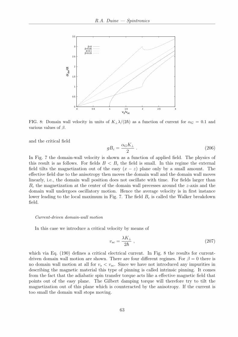
R.A. Duine — Spintronics
0
0.5
1
1.5
2
2.5
3
3.5
0 0.5 1 1.5 2 2.5 3
drdw
/dt
vs/vsc
β=0β=0.05
β=0.1β=0.15
FIG. 8: Domain wall velocity in units of K⊥λ/(2~) as a function of current for αG = 0.1 andvarious values of β.
and the critical field
gBc =αGK⊥
2. (206)
In Fig. 7 the domain-wall velocity is shown as a function of applied field. The physics ofthis result is as follows. For fields B < Bc the field is small. In this regime the externalfield tilts the magnetization out of the easy (x − z) plane only by a small amount. Theeffective field due to the anisotropy then moves the domain wall and the domain wall moveslinearly, i.e., the domain wall position does not oscillate with time. For fields larger thanBc the magnetization at the center of the domain wall precesses around the z-axis and thedomain wall undergoes oscillatory motion. Hence the average velocity is in first instancelower leading to the local maximum in Fig. 7. The field Bc is called the Walker breakdownfield.
Current-driven domain-wall motion
In this case we introduce a critical velocity by means of
vsc =λK⊥2~
, (207)
which via Eq. (190) defines a critical electrical current. In Fig. 8 the results for current-driven domain wall motion are shown. There are four different regimes. For β = 0 there isno domain wall motion at all for vs < vsc. Since we have not introduced any impurities indescribing the magnetic material this type of pinning is called intrinsic pinning. It comesfrom the fact that the adiabatic spin transfer torque acts like a effective magnetic field thatpoints out of the easy plane. The Gilbert damping torque will therefore try to tilt themagnetization out of this plane which is counteracted by the anisotropy. If the current istoo small the domain wall stops moving.
63
R.A. Duine — Spintronics
The second regime is the situation that β < αG. For any β 6= 0 the domain wall isno longer intrinsically pinned. From the equations of motion in Eq. (200) we observe thatthe dissipative spin transfer torque acts like an external magnetic field and hence that thedomain wall velocity initially varies linearly with current.
A special case is the situation that αG = β. In this case we see from Eq. (192) the mag-netization direction is time-independent in the frame moving with velocity vs and thereforethat the domain wall velocity 〈rdw〉 = vs.
The fourth regime is β > αG. In this situation there is Walker-breakdown-like behaviorprecisely because the dissipative spin transfer torque acts like an external magnetic field inthe z-direction.
As a final remark we note that the theory presented so far is valid only at zero temper-ature and in the absence of inhomogeneities in the magnetic material. Development of atheory valid at nonzero temperatures and for more complicated situations, such as the caseof domain-wall-line bending and intrinsic pinning, is an active topic of ongoing research.Furthermore, although there is now some kind of consensus that β 6= αG, it is by no meanssettled — not even experimentally — which values of β one should take for a given materialor what microscopically the most important processes are that contribute to the dissipativespin transfer torque.
Exercises
1. Spin waves with current
Linearize the equation of motion in Eq. (189) to find the spin-wave spectrum in thepresence of electric current (consider only the case that αG = 0 and B = 0). Which criticalcurrent makes the homogeneous ground state unstable?
2. Domain Wall Mass
Consider a ferromagnet with magnetization direction Ω described by the Euclidean action
AE[Ω] =
∫ ~βT
0
dτ
[∫dx
a3i~A(Ω(x, τ)) · ∂Ω(x, τ)
∂τ
]+ E[Ω]
, (208)
with the energy functional
E[Ω] =
∫dx
a3
[−Js
2Ω(x, τ) · ∇2Ω(x, τ) +
K⊥Ω2y
2− KzΩ
2z
2− gBΩz(x, τ)
], (209)
and x ∈ −∞,∞, y ∈ 0, Ly, and z ∈ 0, Lz. In these expressions A(Ω) is the vectorpotential of a magnetic monopole (see Sec. II of the lecture notes), Js the spin stiffness,K⊥, Kz anisotropy constants, and B the magnitude of the external magnetic field.
a) Write Ω = (sin θ cos φ, sin θ sin φ, cos θ) and give the action in terms of θ and φ. (Forthe term that involves A use the results from Sec. II — no calculations!)
64

R.A. Duine — Spintronics
b) Assume that K⊥ À Js(∇φ)2. This means that field configurations with φ(x, τ) largeare suppressed. Expand the action up to quadratic order in φ, ignoring the (∇φ)2-terms. Integrate out the field φ (ignore boundary terms after integrating the actionby parts) and show that the effective action is of the form
AeffE [θ] =
∫ ~βT
0
dτ
∫dx
a3
Js
2
[1
c2
(∂θ(x, τ)
∂τ
)2
+ (∇θ(x, τ))2
]− gB cos θ − Kz
2cos2 θ
.
(210)
Give the expression for the velocity c.
Consider the situation B = 0.
c) Vary the effective action to obtain the equation of motion for θ.
d) Show that the solutionθ(x) = 2 tan−1
(e(x−rdw)/λ
), (211)
is a time-independent solution (λ =√
Js/Kz) of the equation of motion for θ.
e) Convince yourself this solution corresponds to a domain wall centered around rdw.Draw a cartoon showing what type of domain wall it is. In which direction will amagnetic field in the positive z-direction move this domain wall? (No calculations!)
f) Calculate the domain wall energy Edw of this time-independent solution by insertingit into the hamiltonian part of the effective action and integrating out x. Subtract theenergy E0 of the homogeneous ground state to obtain a finite answer (for the variousnasty integrals you may wish to consult Mathematica...).
Consider the situation B 6= 0.
g) Make the position of the domain wall a dynamical variable, i.e., rdw → rdw(τ). Insertthe above domain wall solution into the effective action to obtain an effective actionfor the domain wall coordinate. Show that
AeffE [rdw] =
∫ ~βT
0
dτ
[Mdw
2
(∂rdw(τ)
∂τ
)2
+ V (rdw(τ))
]. (212)
Determine the domain wall position dependence of the potential V (rdw), and the massMdw of the domain wall. This mass is called the Doring mass.
h) Show that Edw = Mdwc2. (Why?)
i) Give the equation of motion for rdw(τ). Does it agree with your answer to part e) ofthis exercise?
Answers: the velocity c =√
K⊥Js/~2 and Mdwc2 = 2LyLz
√JsKz/a
3.
65

R.A. Duine — Spintronics
Additional reading
Selection of theory papers:
• L. Berger, J. Appl. Phys. 55, 1954 (1984).
• G. Tatara and H. Kohno, Phys. Rev. Lett. 92, 086601 (2004).
• S. Zhang and Z. Li, Phys. Rev. Lett. 93, 127204 (2004).
• X. Waintal and M. Viret, Europhys. Lett. 65, 427 (2004).
• S. E. Barnes and S. Maekawa, Phys. Rev. Lett. 95, 107204 (2005).
Some experimental papers:
• P. P. Freitas and L. Berger, J. Appl. Phys. 57, 1266 (1985).
• J. Grollier, P. Boulenc, V. Cros, A. Hamzi, A. Vaurs, A. Fert, and G. Faini, Appl.Phys. Lett. 83, 509 (2003).
• M. Tsoi, R.E. Fontana, and S.S.P. Parkin, Appl. Phys. Lett. 83, 2617 (2003).
• A. Yamaguchi, T. Ono, S. Nasu, K. Miyake, K. Mibu, and T. Shinjo, Phys. Rev. Lett.92, 077205 (2004).
• M. Klaui, C. A. F. Vaz, J. A. C. Bland, W. Wernsdorfer, G. Faini, E. Cambril, L. J.Heyderman, F. Nolting, and U. Rudiger, Phys. Rev. Lett. 94, 106601 (2005).
• G. S. D. Beach, C. Knutson, C. Nistor, M. Tsoi, and J. L. Erskine, Phys. Rev. Lett.97, 057203 (2006).
• M. Hayashi, L. Thomas, C. Rettner, R. Moriya and S. S. P. Parkin, Nature Physics3, 21 (2007).
• M. Yamanouchi, D. Chiba, F. Matsukura, T. Dietl, and H. Ohno, Phys. Rev. Lett.96, 096601 (2006).
This subject is not without controversy. See for example Phys. Rev. Lett. 96, 189702(2006) and Phys. Rev. Lett. 96, 189701 (2006).
66

R.A. Duine — Spintronics
VIII. SPIN HALL EFFECT
In this chapter we consider the so-called spin Hall effect. This name derives from theanalogy with the ordinary hall effect, where there is — in the presence of a magnetic field —a charge current perpendicular to the applied electric and magnetic field due to the Lorentzforce, i.e.,
jc,y = σHEx . (213)
with σH the Hall conductivity. In the example of the spin Hall effect discussed here , wehave that in the absence of a magnetic field
jzs,α = σSHεαβEβ , (214)
where εαβ is the two-dimensional Levi-Civita tensor, so that there is a spin current with spinin the z-direction with spatial component perpendicular to the electric field.
The geometry we consider here is that of a two-dimensional electron gas (2DEG) where(x, y) are coordinates in the two-dimensional plane and z is perpendicular to this plane. Ifthe system does not have inversion symmetry in this latter direction, it follows from Eq. (88)that the effective hamiltonian is the so-called Rashba hamiltonian
H =
(p2
x + p2y
)
2m+ λ (τ × p) · z , (215)
with λ > 0 a spin-orbit coupling constant. Its eigenstates, labelled by an index ∈ +,−,are given by 6
ψ±(x) =1√V
eik·x 1√2
(1
∓ieiθk
)≡ 1√
Veik·xχ±(k) ;
θk = tan−1 kx
ky
. (216)
with energiesEk,± = εk ± ~λk . (217)
The spin Hall effect described in this chapter is the so-called intrinsic spin Hall effect whichis due to effects of spin-orbit coupling in the bandstructure, such as the terms proportional toλ in the above hamiltonian. The extrinsic spin Hall effect is due to spin-dependent disorderscattering and therefore depends on extrinsic properties (such as the disorder potential),and will not be considered here.
The first step towards deriving Eq. (214) is a linear-response expression for the spincurrent in terms of the electric field. Following the procedure described in Appendix A wefind the Kubo formula
jzs,α ≡ 〈Jz
s,α(x, τ)〉 = −1
~
∫ ~β
0
dτ ′∫
dx′〈Jzs,α(x, τ)Jp,β(x′, τ ′)〉0Eβe−iωpτ ′
ωp
+
∫ ~β
0
dτ ′∫
dx′[λ|e|~ωp
e−iωpτ ′εzβγEγ〈Jzs,α(x, τ)φ†(x′, τ ′)τβφ(x′, τ ′)〉0
]. (218)
6 From now on we use x and k for two-dimensional position and momentum.
67
R.A. Duine — Spintronics
In this expression, the first term turns out not to contribute to the spin Hall conductivity.Working out the second term gives
jzs,α =
~2
2m
1
~βV
λ|e|e−iωpτ
~ωp
εzβγEγ
∑
k,n
kαTr[G0(k, iωn)τ zG0(k, iωn + iωp)τ
β]
, (219)
where the trace is over spin space only. The single-electron Green’s function of the Rashbamodel is given by
G0(k, iωn) =∑
δ∈+,−
−~−i~ωn + Ek,δ − µ
χδ(k)χ†δ(k) . (220)
Note that this Green’s function is a matrix in spin space.Performing the sum over Matsubara frequenties results in
jzs,α =
λ|e|e−iωpτ~2
2mωp
εzβγEγ1
V
∑
k;δ,δ′∈+,−
kα
[N(Ek,δ − µ)−N(Ek,δ′ − µ)
Ek,δ − Ek,δ′ + i~ωp
]
×Tr[χδ(k)χ†δ(k)τ zχδ′(k)χ†δ′(k)τβ
], (221)
where the trace in the latter factor is worked out to yield
Tr[χδ(k)χ†δ(k)τ zχδ′(k)χ†δ′(k)τβ
]=
−12i(δ − δ′) cos θk , if β = x ;
−12i(δ − δ′) sin θk , if β = y .
(222)
This result implies that the right-hand side of Eq. (221) is zero if β 6= α. Converting thesum over k to an integral and performing the angular part of it (i.e., the integral over θk)we find
jzs,α =
λ|e|e−iωpτ~2
4mωp
εzβγEγ
∑
δ,δ′∈+,−
∫ ∞
0
dkk2
[N(Ek,δ − µ)−N(Ek,δ′ − µ)
Ek,δ − Ek,δ′ + i~ωp
]i
2(δ′ − δ) .(223)
Taking the ωp → 0 limit yields
jzs,α =
λ|e|~3
8mεzβγEγ
∑
δ,δ′∈+,−
∫ ∞
0
dkk2
[N(Ek,δ − µ)−N(Ek,δ′ − µ)
(Ek,δ − Ek,δ′)2
](δ′ − δ) . (224)
Since only the δ 6= δ′ part contributes to the above sum we immediately have that
jzs,α = − |e|~
16mλεzβγEγ
∫ ∞
0
dk [N(Ek,+ − µ)−N(Ek,− − µ)] , (225)
where we used that (Ek,δ − Ek,δ′)2 = 4λ2~2k2 for δ 6= δ′. Note that from the above result it
is clear that the entire Fermi sea contributes to the spin Hall conductivity, and not just theelectrons at the Fermi level.
Next, we take the zero-temperature limit and choose the Fermi energy such that it crossesboth bands. We then have that kF− − kF+ = 2mλ/~ so that
jzs,α = − |e|~
16mλεzβγEγ
∫ ∞
0
dk [N(Ek,+ − µ)−N(Ek,− − µ)]
= − |e|~16mλ
εzβγEγ(kF+ − kF−) =|e|8π
εzβγEγ =|e|8π
εαβEβ , (226)
68

R.A. Duine — Spintronics
which finally yields the desired result for the spin Hall conductivity [compare Eq. (214)]
σSH =|e|8π
. (227)
The above result implies that for this model the spin Hall conductivity does not depend onsystem parameters, and is therefore called universal. Note also that the spin Hall conduc-tivity is not infinite in the absence of disorder, contrary to the electric conductivity. Thisis related to the fact that the spin Hall conductivity is a reactive transport coefficient, i.e.,it relates two quantities (spin current and electric field) that have the same sign upon timereversal. This is different from the electrical conductivity that is by definition dissipative,since relates a quantity (the electric field) that does not change sign upon time reversal, tothe electric current that does change sign. That the electrical conductivity is dissipative isunderstood, as electric current results in heating associated with dissipation of the current.
Exercises
1. Rashba model
Consider a two-dimensional electron gas (2DEG) described by the Rashba Hamiltonian:
H =
(p2
x + p2y
)
2m+ λ(τ × p) · z ,
with λ > 0. Here p = (px, py, pz) is the momentum operator and τ is the vector of the Paulimatrices. Finally, ez is the unit vector in the z-direction.
a) Give the eigenvalues and eigenfunctions of the hamiltonian.
b) Calculate the expectation value of the spin operator S = ~τ/2 for these eigenfunctions.
c) Consider a single electron with two-component wave function ψ(x, t). Using theSchrodinger equation and the definition
−|e| ∂∂t
[ψ(x, t)†ψ(x, t)
] ≡ −∇ · Jc ,
of the charge current, determine the expression for the charge current in terms of thewave function.
d) Using the Schrodinger equation, express d〈τ 〉/dt in terms of an expectation value ofthe spin current operator Jµ
α = ~pατµ/(2m).
e) Repeat the above for the so-called Dresselhaus hamiltonian
H =p2
2m+ α (pyτ
y − pxτx) .
69

R.A. Duine — Spintronics
Additional reading
Theoretical papers discussing the spin Hall effect:
• Shuichi Murakami, Naoto Nagaosa, and Shou-Cheng Zhang, Science 301, 1348 (2003).
• Jairo Sinova, Dimitrie Culcer, Q. Niu, N. A. Sinitsyn, T. Jungwirth, and A. H. Mac-Donald, Phys. Rev. Lett. 92, 126603 (2004).
• Review by J. Schliemann available at: http://arxiv.org/abs/cond-mat/0602330.
Experimental paper about the spin Hall effect:
• Y.K. Kato, R.C. Myers, A.C. Gossard, and D. D. Awschalom, Science 306, 1910(2004).
• J. Wunderlich, B. Kaestner, Jairo Sinova, and T. Jungwirth, Phys. Rev. Lett. 94,047204 (2005).
It turns out that if you add disorder then σSH = 0 within the model presented here! Thiswas shown in
• J.I. Inoue, G.E.W. Bauer, and L.W. Molenkamp, Phys. Rev. B, 70, 041303 (2004).
70

R.A. Duine — Spintronics
IX. ACKNOWLEDGEMENTS
It is a pleasure to thank all the students who took “spintronics” in Spring 2007 for findingmany typos in earlier versions of this manuscript.
71
R.A. Duine — Spintronics
APPENDIX A: ELECTRONIC TRANSPORT
Electronic transport is a large and complicated subtopic of condensed-matter physics. Inthis appendix we sketch some results. Various length scales are important:
• The De Broglie wavelength `dB.
• The phase-coherence length `ϕ: this is roughly speaking the length scale over whichthe electron “forgets about” its quantummechanical phase. Microscopic processes thatlead to loss of phase coherence involve exchange of energy, i.e., inelastic processes.After a collision with an energy exchange δε the electron picks up a phase factoreiδεt. Averaging over such processes “washes out” the quantummechanical phase ofthe electron.
• The mean free path `0, corresponding to the average distance travelled between twoscattering events by an electron with the Fermi velocity. Since elastic scattering eventscontribute to `0 but not to `ϕ we have that `ϕ 6= `0 in general. The scattering time isdefined by τsc = `0/vF .
Here we consider two models: Landauer-Butikker theory and Boltzmann transport theory.Landauer-Butikker theory applies for phase-coherent ballistic transport, i.e., when `ϕ, `dB
and `0 are of the order of the system size. Boltzmann theory holds in the opposite limitprovided the scattering is weak so that τscεF /~À 1.
Landauer-Butikker formalism
In Landauer-Butikker theory we imagine a small system coupled to leads on the left andright, with lead chemical potentials µL and µR, respectively. We assume µL > µR so thatelectrons flow from left to right lead. In the Landauer-Butikker formalism we solve theSchrodinger equation in the system. This leads to transmission probablities Tσ(ε) = |tσ(ε)|2for a scattering state with energy ε and spin state |σ〉, in terms of the transmission amplitudetσ(ε). The current through the system is for one spin state and in one dimension given by
Iσ = − |e|2π~
∫dεTσ(ε) [N(ε− µL)−N(ε− µR)] . (A1)
It follows that the polarization of the current is given by
P =T↑(εF )− T↓(εF )
T↑(εF ) + T↓(εF ). (A2)
Boltzmann transport theory
In Boltzmann transport theory we imagine a large homogeneous (up to disorder) systemin which the current is induced by an electric field E. The goal is to calculate the inducedtransport current in linear response, i.e.,
jc ≡ 〈Jc〉 = σeE , (A3)
72

R.A. Duine — Spintronics
which defines the conductivity σe.This is done by using a Boltzmann equation. The Boltzmann equation is in this case
an equation for the distribution function f(k, t) such that f(k, t)dk/(2π)3 is the number ofelectrons with momentum in the interval [k,k + dk]. First, we assume that there are nocollisions. Because the number of electrons is conserved we have that
f(k, t) = f(k + k∆t, t + ∆t) , (A4)
where ∆t is a small time step. From this, we find by linearizing in ∆t that
∂f
∂t+
∂f
∂k· k = 0 , (A5)
which is a continuity-like equation in momentum space. The semi-classical dynamics of theelectron is determined by
~k = −|e|E , (A6)
which, together with Eq. (A5) results in the collisionless Boltzmann equation
∂f
∂t− |e|E
~· ∂f
∂k= 0 . (A7)
This equation simply describes the acceleration of all electrons in the electric field and istherefore not sufficient to reproduce a finite conductivity. Moreover, in the long-time limitit does not determine the limiting behaviour of the distribution function. For example, forE = 0 the equilibrium distribution should be the Fermi-Dirac distribution function.
The solution is to add collision terms to the right-hand side of the Boltzmann equationsuch that
∂f
∂t− |e|E
~· ∂f
∂k= Γcoll[f ] , (A8)
where the collision terms should be such that Γcoll[N ] = 0, that is, they are zero for theFermi-Dirac distribution. Moreover, they should be such that in the absence of externalfields f(k, t →∞) → N(εk − µ), so that the system relaxes to the Fermi-Dirac equilibriumdistribution function.
Every physical process, such as electron-electron interactions, electron-phonon interac-tions, and so on, brings about a distinct collision term in the Boltzmann equation. Here wefocus on elastic scattering in the so-called relaxation time approximation which is describedby
Γcoll[f ] = − 1
τsc
[f(k, t)−N(εk − µ)] , (A9)
where τsc is the phenomenological relaxation time. In the absence of an external field adeviation δf(k, t) behaves as δf(k, t) ∝ e−t/τsc so that the distribution function relaxes tothe Fermi-Dirac distribution function on the time scale τsc.
Solving the Boltzmann equation for the steady-state situation we find that, to first orderin the electric field E, the deviation of the distribution function from equilibrium is at lowtemperature given by
δf(k) =|e|τscE
~· ∂N(εk − εF )
∂k. (A10)
73
R.A. Duine — Spintronics
From this one finds that the current (the factor of two is for spin)
jc = −2|e|∫
dk
(2π)3[N(εk − εF ) + δf(k)]vk = σeE , (A11)
with vk = ∂ε∂(~k)
the velocity of an electron with wave number k, and where the conductivity
is (for kBT ¿ εF )
σe =n|e|2τsc
m, (A12)
with n the total electron density. This result is called the Drude conductivity.In case there is no spin degeneracy, for example, due to exchange splitting, we have that
jσ =nσ|e|2τσ,sc
mE , (A13)
where nσ is the density of electrons with spin σ and m is the electron mass. The total chargecurrent
jc = j↑ + j↓ ,
so that the current polarization factor
P =n↑τ↑,sc − n↓τ↓,scn↑τ↑,sc + n↓τ↓,sc
.
Exercise: Boltzmann equation and conductivity
a) Derive Eq. (A12) .
b) Now consider the electron system in two dimensions with a perpendicular magneticfield B. This implies that Eq. (A6) changes to
~k = −|e|E− m|e|~
k×B .
The conductivity σe, defined by jc = σe · E is now a 2 × 2 matrix with nonzero off-diagonal components. Calculate this matrix and in particular its off-diagonal compo-nents, that describe the Hall effect. Calculate also the resistivity defined by ρ = σ−1.
c) Consider again the Boltzmann equation in three dimensions without magnetic field,but with electric field, and with the collision term in Eq. (A9). We solve this equationby making the ansatz
f(k, t) = N(εk−mvd(t)
~− µ
),
where the drift velocity vd(t) is now the parameter for which we want to derive anequation of motion. Show that
nvd(t) = −n|e|Em
− Γ(vd(t)) ,
where
Γ(vd) =1
τsc
∫dk
(2π)3
~km
[N
(εk−mvd(t)
~− µ
)−N (εk − µ)
].
74
R.A. Duine — Spintronics
d) Linearize the equation of motion for small vd(t) and show that, using jc = −n|e|vd,you ultimately obtain the result in Eq. (A12) for the conductivity σe .
e) Consider now the case without elastic disorder-potential scattering scattering (τsc →∞), but with electron-electron scattering, so that
Γcoll[f ] =2π
~U2
∫dk2
(2π)3
∫dk3
(2π)3
∫dk4
(2π)3(2π)3δ(k + k2 − k3 − k4)δ (εk + εk2 − εk3 − εk4)
×[1− f(k, t)] [1− f(k2, t)] f(k3, t)f(k4, t)
−f(k, t)f(k2, t) [1− f(k3, t)] [1− f(k4, t)] , (A14)
where the electron-electron interaction is approximated by V (x− x′) = Uδ(x− x′). Derivethe equation of motion for vd(t) with the above collision integral and show that Γ(vd) = 0.Explain that this implies 1/σe = 0. Explain why electron-electron interactions do not leadto a finite conductivity.
A generalization of the collision integral in Eq. (A9) is to let the probability amplitudeTk,k′ for elastic scattering from k → k′ depend on the momenta, so that
Γcoll[f ] = −∫
dk′
(2π)3|Tk,k′|2δ(εk − εk′) [f(k, t)− f(k′, t)] , (A15)
where the energy-conserving δ-function implements the elasticity of the collision of the elec-tron with the disorder potential. It is common to introduce a momentum-dependent relax-ation time τsc(k, θ) by writing
∫dk′
(2π)3|Tk,k′|2δ(εk − εk′) ≡
∫ π
0
dθ sin θ1
2τsc(k, θ), (A16)
where1
2τsc(k, θ)=
1
(2π)2
mk
~2|T (k, θ)|2 , (A17)
and where we put |Tk,k′|2 = |T (k, θ)|2 and we assumed that this scattering probability onlydepends k and on the angle θ between k and k′. We now solve the linearized version of theBoltzmann equation using the collision integral in Eq. (A15), and by making the ansatz
δf(k) =|e|τtrE
~· ∂N(εk − εF )
∂k, (A18)
where the so-called transport relaxation time τtr is to be determined. From this we find that
1
τtr
=
∫ π
0
dθ sin θ1
2τsc(k, θ)[1− cos θ] , (A19)
and
σe =n|e|2τtr
m. (A20)
This shows that the transport relaxation time τtr, that determines the decay of the electriccurrent, is in general not equal to the scattering time τsc, which roughly corresponds to thelifetime of a state with a given momentum. Note that that in the case that the scatteringis angle-independent, i.e., Tk,k′ = T (k, k′) we have that τtr = τsc.
Reproducing these results using quantummechanical linear response theory turns out tobe quite complicated, as we sketch in the next sections.
75

R.A. Duine — Spintronics
Linear-response theory
For simplicity, we ignore the electron spin for now. The goal is to calculate, to first orderan homogeneous electric field E, the expectation value of the electric current, Eq. (148), inthis case given by
Jc(x, τ) = − |e|~2mi
[φ∗(x, τ)∇φ(x, τ)− (∇φ∗(x, τ)) φ(x, τ)]− |e|2mc
Aem(x, τ)φ∗(x, τ)φ(x, τ)
≡ Jp(x, τ) + Jd(x, τ) , (A21)
where the diamagnetic current Jd(x, τ) contains the contribution due to the vector potential.We choose the London gauge
Vem(x, τ) = 0 ;
Aem(x, τ) =−cE
ωp
e−iωpτ , (A22)
where the limit of the photon frequency ωp → 0, to be taken at the end of the calculation,is implied. The action for the system is now given by
AE[φ∗, φ,E] =∫ ~βT
0
dτ
∫dxφ∗(x, τ)
[~
∂
∂τ+
1
2m
(−i~∇− |e|E
ωp
e−iωpτ
)2
− µ + Vd(x)
]φ(x, τ) ,
(A23)
with Vd(x) a disorder potential to be discussed in more detail later on. The action is nowseparated into a part with the electric field, and without, so that
AE[φ∗, φ,E] = Ad[φ∗, φ] +
∫ ~βT
0
dτ
∫dxJp(x, τ) · E
ωp
e−iωpτ , (A24)
where
Ad[φ∗, φ] =
∫ ~βT
0
dτ
∫dxφ∗(x, τ)
(~
∂
∂τ− ~
2∇2
2m− µ + Vd(x)
)φ(x, τ) , (A25)
and quadratic terms in E are already neglected.The expectation value of the current is now given by
jc,α ≡ 〈Jc,α(x, τ)〉 ≡ 1
Z
∫d[φ∗]d[φ] [Jp,α(x, τ) + Jd,α(x, τ)] e
−Ad/~−∫ ~βT0 dτ
∫dxJp(x,τ)· E
~ωpe−iωpτ
= 〈Jd,α(x, τ)〉d −∫ ~βT
0
dτ ′∫
dx′〈Jp,α(x, τ)Jp,β(x′, τ ′)〉d Eβ
~ωp
e−iωpτ ′ , (A26)
to linear order in E. The expectation value 〈· · ·〉d is taken with respect to the action inEq. (A25) and is normalized to the partition function Z corresponding to this action. Theabove formula shows that the non-equilibrium expectation value of an operator, to first order
76
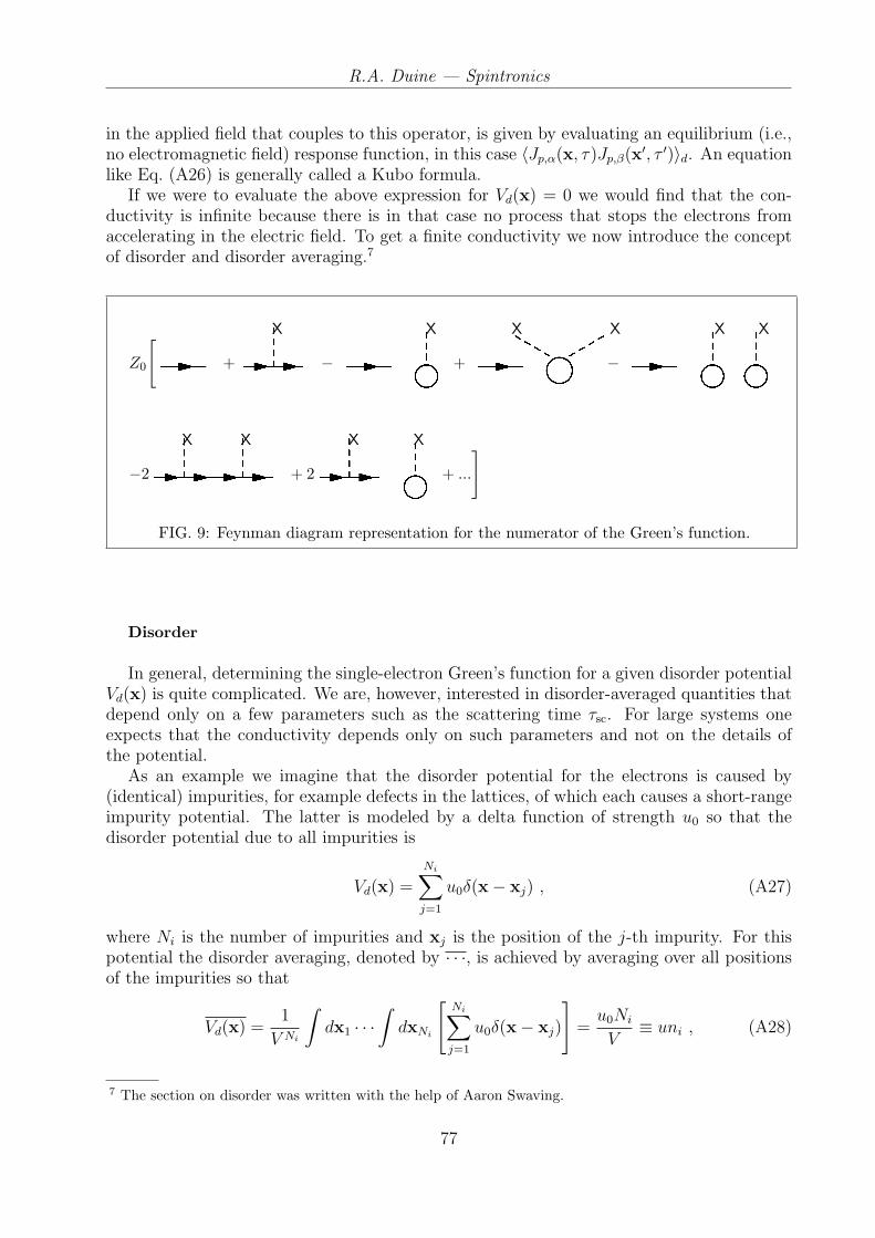
R.A. Duine — Spintronics
in the applied field that couples to this operator, is given by evaluating an equilibrium (i.e.,no electromagnetic field) response function, in this case 〈Jp,α(x, τ)Jp,β(x′, τ ′)〉d. An equationlike Eq. (A26) is generally called a Kubo formula.
If we were to evaluate the above expression for Vd(x) = 0 we would find that the con-ductivity is infinite because there is in that case no process that stops the electrons fromaccelerating in the electric field. To get a finite conductivity we now introduce the conceptof disorder and disorder averaging.7
X X X X X X
Z0
[ + −+−X X X X
−2 + 2+ ...
]
FIG. 9: Feynman diagram representation for the numerator of the Green’s function.
Disorder
In general, determining the single-electron Green’s function for a given disorder potentialVd(x) is quite complicated. We are, however, interested in disorder-averaged quantities thatdepend only on a few parameters such as the scattering time τsc. For large systems oneexpects that the conductivity depends only on such parameters and not on the details ofthe potential.
As an example we imagine that the disorder potential for the electrons is caused by(identical) impurities, for example defects in the lattices, of which each causes a short-rangeimpurity potential. The latter is modeled by a delta function of strength u0 so that thedisorder potential due to all impurities is
Vd(x) =
Ni∑j=1
u0δ(x− xj) , (A27)
where Ni is the number of impurities and xj is the position of the j-th impurity. For thispotential the disorder averaging, denoted by · · ·, is achieved by averaging over all positionsof the impurities so that
Vd(x) =1
V Ni
∫dx1 · · ·
∫dxNi
[Ni∑j=1
u0δ(x− xj)
]=
u0Ni
V≡ uni , (A28)
7 The section on disorder was written with the help of Aaron Swaving.
77

R.A. Duine — Spintronics
where ni is the density of impurities. For future purposes we also need
Vd(x)Vd(x′) = n2i u
20 + niu
20δ(x− x′) , (A29)
which holds for Ni À 1. For convenience, we shift the single-electron energies with Vd(x) so
that we are from now on dealing with a disorder potential δVd(x) ≡ Vd(x)− Vd(x) which ison average zero and has correlations
δVd(x)δVd(x′) = niu20δ(x− x′) , (A30)
We first calculate the electron Green’s function G(x, τ ;x′τ ′) which is given by
−G(x, τ ;x′, τ ′) =1
Z
∫d[φ∗]d[φ]φ(x, τ)φ∗(x′, τ ′) exp
−1
~Ad[φ
∗, φ]
. (A31)
Both the numerator and the denominator Z are calculated in perturbation theory in δVd(x).For the numerator we have that
∫d[φ∗]d[φ]φ(x, τ)φ∗(x′, τ ′)e−
1~
∫ ~βT0 dτ
∫dxφ∗(x,τ)
(~ ∂
∂τ−~2∇2
2m−µ
)φ(x,τ)
×(
1− 1
~
∫ ~βT
0
dτ ′′∫
dx′′φ∗(x′′, τ ′′)δVd(x′′)φ(x′′, τ ′′)
+1
2~2
∫ ~βT
0
dτ ′′∫
dx′′∫ ~βT
0
dτ ′′′∫
dx′′′φ∗(x′′, τ ′′)δVd(x′′)φ(x′′, τ ′′)φ∗(x′′′, τ ′′′)δVd(x
′′′)φ(x′′′, τ ′′′)
+ · · ·)
. (A32)
In working out this expression using Wick’s theorem we encounter terms likeδVd(x)G0(x, τ ;x′τ ′) where G0 is the Green’s function without disorder. These are depictedusing Feynman diagrams, by using a solid line with arrow for the Green’s function, andusing a dashed line ending at a × for the disorder potential. To second order in the disorderpotential the numerator is given in Fig. 9. The denominator of the Green’s function, i.e.,the partition function Z is given in Feynman diagram language in Fig. 10. Taking the ratioof these two expressions cancels the disconnected diagrams as usual and leaves use with theconnected ones depicted in Fig. 11.
X X X X X
Z0
[1−−+]
FIG. 10: Feynman diagram representation for the partition function.
78

R.A. Duine — Spintronics
X X X
G = + +FIG. 11: Feynman diagram representation of the electron Green’s function.
Upon taking the disorder average of the expression for the Green’s function to secondorder in the disorder potential, the first-order term vanishes. Because of the delta-functioncorrelations (see Eq. (A30)) the spatial coordinates of the disorder potential are now con-nected. This depicted by connected the two dashed lines to the same ×. This results in theFeyman diagrams in Fig. 12. Note that after the disorder averaging there appears an effec-tive interaction, which is local in space but nonlocal in time. This interaction correspondsto ∫ ~βT
0
dτ
∫ ~βT
0
dτ ′∫
dxniu
20
~φ∗(x, τ)φ∗(x, τ ′)φ(x, τ ′)φ(x, τ) .
However, one has to be careful when treating disorder by doing perturbation theory inthis interaction. Since all disorder-averaged diagrams for the Green’s function follow fromconnected ones, like in Fig. 11, all diagrams should be irreducible upon cutting the linescorresponding to the above effective interaction.
X
G = + + ...
FIG. 12: Feynman diagram representation for the disorder-averaged Green’s function.
We introduce the self-energy by writing the Green’s function as
G = G0 + G0 · Σ ·G0 + · · · = G0 + G0ΣG , (A33)
where the multiplication · implies integration over position and imaginary time. The self-energy is then, to second order in δVd(x, τ) which is called the Born approximation, givenby
~Σ(x, τ ;x′, τ ′) =1
~niu
20G0(x, τ ;x′, τ ′)δ(x− x′). (A34)
It’s Fourier transform
~Σ(iωn) =
∫d(τ − τ ′)
∫d(x− x′)e−ik·(x−x′)+iωn(τ−τ ′) 1
~niu
20G0(x, τ ;x′, τ ′)δ(x− x′)
= niu20
∫dk
(2π)3
1
i~ωn − εk + µ, (A35)
79
R.A. Duine — Spintronics
is momentum independent. For small temperatures, so that µ → εF , the self-energy isevaluated as
~Σ(iωn) = niu20
∫dk
(2π)3
1
i~ωn − εk + µ= niu
20
∫dk
(2π)3
1
i~ωn − (εk − εF )
= ~Σ(0) + niu20
∫dk
(2π)3
[1
i~ωn − (εk − εF )+
1
εk
]
= ~Σ(0) + niu20π
1
2π2
m
~2
√2m
~2
√−εF − i~ωn ' ~Σ(0)− πiniu
20ν(εF )sign(ωn)
≡ ~Σ(0)− i~
2τsc
sign(ωn) . (A36)
In the above expression, the frequency-independent part of the self-energy ~Σ(0) ∼− ∫
dk/εk is real and diverges for large momenta, i.e., has an ultraviolet divergence. Thisdivergence is due to taking the impurity potential to be delta-function-like. We absorbthis divergent contribution in the chemical potential and ignore it in the following. Thesign-function in the above results from the branch cut in the square root and taking thesmall-frequency limit. The scattering time is found as
~τsc
= 2πniu20ν(εF ) . (A37)
This scattering time determines the decay of an electron in a plane wave state due to scat-tering with impurities, which can also be seen by realizing that the decay rate correspondingto this process is the imaginary part of Σ(ω+) which leads to Fermi’s Golden Rule. Withthis result the disorder-averaged Green’s function is
G(k, iωn) =~
i~ωn − (εk − µ)− ~Σ(iωn). (A38)
Exercise: calculations with the disorder-averaged Green’s functionConsider the expression for the expectation value of the current in Eq. (A26).
a) Take Vd(x) = 0 in first instance and show, by using Wick’s theorem and Fouriertransformation that
jc,α =n|e|2Eαe−iωpτ
mωp
+|e|2e−iωpτ
m2βV ωp
∑
k,n
EβkαkβG0(k, iωn)G0(k, iωn − iωp) , (A39)
with G0(k, iωn) the Green’s function in the absence of disorder.
b) Show that the ωp → 0 divergence of the first term of Eq. (A39) is precisely cancelledby the second term.
With disorder we have seen that the Green’s function is given by
G(k, iωn) =1
iωn − (εk−µ)~ + i
2τscsign(ωn)
. (A40)
80

R.A. Duine — Spintronics
c) Show that
G(+)
(x− x′) ≡ 1
V
∑
k
G(k, ω+ = 0)eik·(x−x′) ,
contains a factor e−|x−x′|/(2`), with ` = vF τsc the mean free path.
d) Consider the second term in Eq. (A39) but with G0 replaced by G. Draw the Feynmandiagrams corresponding to this contribution to the current-current response function.
e) Show that
1
V
∑
k,n
kαkβG(k, iωn)G(k, iωn − iωp) =1
3ν(εF )k2
F δαβ~β~ωp
ωp + 1τsc
,
and that this leads to σe = n|e|2τsc/m in combination with Eq. (A39) and the resultof part a). Hint: use that
∫dk
(2π)3kαkβG(k, iωn)G(k, iωn − iωp) '
1
3ν(εF )k2
F δαβ
∫ ∞
−∞dε
1
iωn − ε~ + i
2τscsign(ωn)
1
iωn − iωp − ε~ + i
2τscsign(ωn − ωp)
.
We end this section by noting that in case one makes the replacement u0δ(x) → u(x) forthe potential due to a single impurity, one finds that the self energy in the Born approxima-tion is given by
~Σ(k, iωn) =ni
V
∑
k′|u(k− k′)|2 1
i~ωn − (εk′ − εF ), (A41)
with u(k) the Fourier transform of u(x). The scattering time is now given by
1
2τsc(k)= −Im
[Σ(+)(k, 0)
],
which, following the steps in the above exercise, leads to σe = n|e|2τsc(kF ). This final resultis incorrect (except if the potential due to a single impurity is a delta function!), as weexpect a Drude formula with a transport relaxation time involving the 1− cos θ factor. Thisshortcoming is repaired by considering vertex corrections to the current-current correlationfunction.
Additional reading
• Notes by P. Coleman are available at
http://www.physics.rutgers.edu/~coleman/mbody/pdf/bk.pdf
.
• Notes by C. Nayak are available at
http://www.physics.ucla.edu/~nayak/many_body.pdf
.
81


![Spintronics [EDocFind.com]](https://img.dokumen.tips/doc/110x75/577d2e0b1a28ab4e1eaea99b/spintronics-edocfindcom.jpg)