Spillovers from Public Intangibles

Cecilia Jona Lasinio (LUISS Lab and ISTAT, Italy), Carol Corrado (The Conference Board,

United States), and Jonathan Haskel (Imperial College, United Kingdom)

Paper prepared for the 34

th IARIW General Conference

Dresden, Germany, August 21-27, 2016

Session 7C: Explaining Productivity Trends II

Time: Friday, August 26, 2016 [Morning]

Spillovers from Public Intangibles

By Carol Corrado∗, Jonathan Haskel†, Cecilia Jona-Lasinio‡§

Draft: August 5, 2016

This paper sets out a framework for the analysis of spillovers to public investments,

tangible and intangible. We exploit a new cross-country industry-level growth

accounting database that includes data on intangible investment for the total

economy, i.e., covering both market and nonmarket activity at the industry level

for 9 EU countries and the United States from 1995 through 2013. Using R&D

investment time series newly developed for national accounts, we find support for

earlier findings in the literature (e.g., Guellec and Van Pottelsberghe de la Potterie

2002, 2004) that there are spillovers from public sector R&D to market sector

productivity. We also find that market sector investments in nonR&D intangible

capital generate spillovers to productivity, raising new possibilities for the analysis

of policies that might boost economic growth.

JEL: O47, E22, E01

Keywords: productivity growth, intangibles, spillovers, R&D, public sector

I. Introduction

The global productivity slowdown has generated renewed interest in policies that might

boost economic growth. One area of interest is spillovers from public sector investments.

The public sector is a major investor in intangible assets, especially human and scientific

knowledge capital via its public investments in education and R&D. The public sector

also is a major investor in tangible assets such as transportation and telecommunications

infrastructures. Investments in these assets, both tangible and intangible, are believed to

exert positive macroeconomic effects in the long run.

Regarding intangibles, the analysis of public sector spillovers in OECD countries typically

looks (in isolation) at R&D and education. Spillovers from publicly performed R&D to mar-

ket sector productivity were studied by, e.g., Guellec and Van Pottelsberghe de la Potterie

(2002, 2004), who found strongly positive effects in their cross-country work. The authors

∗ The Conference Board and Center for Business and Public Policy, McDonough School, Georgetown University† Imperial College, London, CEPR and IZA‡ ISTAT and LLEE, Rome§ We thank Ana Rincon-Aznar for excellent assistance and are grateful to the European Commission FP-7 grant

agreement 612774 (SPINTAN) for support.

1

2

also investigated interrelationships among sector funding, performance, and research pur-

pose of the R&D. The literature on the positive effects of R&D is extensive but largely

pertains to R&D that is privately performed (yet possibly publicly funded).1 Some of the

nuances in this literature discussed in more detail when setting out the models and empirics

used to study R&D spillovers in this paper, which we believe to be the first re-examination

of these issues using national accounts R&D data.

Spillovers from education to economic growth have also been studied extensively, and a

recent study found strong evidence of growth spillovers from human capital accumulation

measured as increases in the skill composition of a country’s labor force using a growth

accounting dataset of 10 major European countries from 1998 to 2007 (Corrado, Haskel,

and Jona-Lasinio, 2013). Moretti (2004b,a) also finds spillovers to education using plant

and state-level data for the United States. Previous work on this topic concluded that, after

accounting accounting for private returns by different worker types, there were no spillovers

to human capital (Inklaar, Timmer, and van Ark, 2008) or argued that spillovers to human

capital accumulation could not be found in cross-country growth regressions because they

were obscured by measurement error (Krueger and Lindahl, 2001). Results are thus highly

variable and therefore revisited in this paper using a richer database than available in

previous work.

Regarding the scope the work in this paper there are a number of points. First, spillovers

from public sector R&D are of course but one dimension of possible spillovers from invest-

ments in knowledge/intangible assets. For example, O’Mahony and Riley (2012) examine

whether employer-provided training may facilitate the generation of spillovers from edu-

cation. Their results support the assumption that spillovers from education within broad

sectors are stronger when employers engage in training and suggest the need to examine

the possibility of multiple channels and also interactive mechanisms whereby intangible as-

sets might impact growth. Complementarities between private ICT investment and private

intangible investment (even when software is included in ICT) have been demonstrated in

prior work (Brynjolfsson, Hitt, and Yang, 2002; Corrado, Haskel, and Jona-Lasinio, 2016a).

Second, besides the well documented spillovers from the conduct of corporate R&D, there

might be pure spillovers from business investments in nonR&D intangibles; these forms of

investments have grown dramatically in relative importance in the United States since the

late 1970s (Corrado and Hulten, 2010). The empirical analysis of spillovers from nonR&D

intangibles is a relatively new, largely unexplored territory. Previous work (Corrado et al.,

2013) found evidence of productivity spillovers to increases in intangible capital excluding

software by market sector industries, again in 10 major European economies over the years

1See Hall, Mairesse, and Mohnen (2009) and Eberhardt, Helmers, and Strauss (2013) for reviews.

3

1998 to 2007. The findings were robust to whether R&D was included or excluded intan-

gibles and thus consistent with an underlying mechanism producing a growth dividend to

private investment in nonR&D intangibles. This finding is revisited in this paper using

additional controls and additional data.

To examine the possible spillovers between public sector intangibles and business sector

productivity performance, this paper looks at the correlation between TFP growth and

different measures of public sector knowledge creation using a new cross-country industry-

level database that includes data on both market and nonmarket intangible investment at

the industry level. Nonmarket intangible investment refers to intangible investments by

governments and nonprofit institutions as estimated by the SPINTAN FP7.2 Market sector

intangibles are from an imminent update to INTAN-Invest, which includes national accounts

estimates of intangible investment for R&D and other intellectual property products capi-

talized in national accounts (software and databases, mineral exploration, and artistic and

entertainment originals), as well as investments in intangible assets not covered in national

accounts.3 Non-national accounts intangibles include design, brand, and organizational

capital, including firm capital generated by employer-provided training.

Growth accounts extended to include non-national accounts intangibles are estimated for

11 EU economies and the United States at the two-digit NACE industry level (with certain

industries further disaggregated according to institution sector, i.e., market and nonmarket)

from 1995 to 2013. For these accounts, capital stocks are built from raw investment data;

ICT deflators are harmonised to U.S. official ICT deflators; and non-market rates of return

are imputed. For further information and analysis of the implications of this dataset, see

Corrado, Haskel, Jona-Lasinio, Iommi, and Mahony (2016).

To preview our results, on this new dataset, we find evidence of spillovers from public

sector R&D to productivity in the market sector. The current version of the dataset does

not include disaggregate information on labor input yet, so our results are incomplete in

this regard. Our earlier finding of spillovers to private nonR&D intangible capital holds in

the extended dataset, i.e., it is robust to the inclusion of the United States in the countries

studied, extension of the time period to cover the financial crises, and inclusion of public

R&D as an additional control.

The rest of the paper sets out a framework (section 2), shows some data (section 3) and

some econometric results (section 4). A final section concludes.

2 Corrado, Haskel, and Jona-Lasinio (2016b) set out the framework for defining and analyzing public intangiblesand Bacchini et al. (2016) set out the methods used to measure investment in the assets included in the dataset usedin this paper; for further information and other working papers, see www.spintan.net.

3INTAN-Invest is an unfunded research initiative that periodically provides intangible investment estimates for22 EU countries, the United States, and Norway see www.intan-invest.net for further details. The forthcomingINTAN-Invest update is previewed in Iommi, Corrado, Haskel, and Jona-Lasinio (2016).

4

II. Framework and existing literature

A. Definitions

Suppose that industry value added in country c, industry i and time t, Qc,i,t can be

written as:

(1) Qc,i,t = Ac,i,tFc,i(Lc,i,t,Kc,i,t, Rc,i,t)

On the right-hand side, L and K are labour and tangible capital services; likewise R is

the flow of intangible capital services and A is a shift term that allows for changes in the

efficiency with which L, K and R are transformed into output. L, K and R are represented

as services aggregates because in fact many types of each factor are used in production. We

will introduce some key distinctions among factor types in a moment. Log differentiating

equation (1) per Solow (1957) gives:

(2) ∆lnQc,i,t = εLc,i,t∆lnLc,i,t + εKc,i,t∆lnKc,i,t + εRc,i,t∆lnRc,i,t + ∆lnAc,i,t

where εX denotes the output elasticity of an input X, which in principle varies by input,

country, industry and time.

To empirically investigate the role of intangibles as drivers of growth starting from the

existing literature, we take two steps. First, consider the ε terms. For a cost-minimizing

firm we may write

(3) εXc,i,t = sXc,i,t, X = L,K,R

where sX is the share of factor X’s payments in value added. The substitution of sXc,i,t for

εXc,i,t in (2) then expresses the first-order condition of a firm in terms of factor shares and

assumes firms have no market power over and above their ability to earn a competitive

return from investments in intangible capital.

Now suppose a firm can benefit from the L, K or R in other firms, industries, or countries.

Then, as Griliches (1979, 1992) notes the industry elasticity of ∆lnR on ∆lnQ is a mix of

both internal and external elasticities so that we can write following Stiroh (2002)

(4) εXc,i,t = sXc,i,t + dXc,i,t, X = L,K,R

which says that output elasticities equal factor shares plus d, where d is any deviation of

elasticities from factor shares due to e.g., spillovers.

5

To examine spillovers, that is d > 0, we note that following Caves, Christensen, and

Diewert (1982) a Divisia ∆lnTFP index can be constructed that is robust to an underlying

translog production function such that we can write (2) as

(5) ∆lnTFPQc,i,t = dLc,i,t∆lnLc,i,t + dKc,i,t∆lnKc,i,t + dRc,i,t∆lnRc,i,t + ∆lnAc,i,t

where ∆lnTFPQc,i,t is calculated as

(6) ∆lnTFPQc,i,t = ∆lnQc,i,t − sLc,i,t∆lnLc,i,t − sKc,i,t∆lnKc,i,t − sRc,i,t∆lnRc,i,t

From (5) therefore, a regression of ∆lnTFPQ on the inputs recovers the spillover terms.

Note that such terms might arise due to imperfect competition/increasing returns not fully

accounted for by the inclusion of intangible capital or translog approximation, and we will

also not be able to distinguish between pecuniary and non-pecuniary returns (Griliches,

1992) and thus use the term “spillovers” for convenience.

B. Existing literature

Some existing papers work with economy-wide data and rather few capitalise R&D. Thus

they use an aggregate value added output term, V , without R&D capitalized and write

down

∆ ln (V/H)c,t = sV,Lc,t ∆ lnL/Hc,t + sV,Kc,t ∆ ln(K/H)c,t + εRc,t∆ lnRc,t + ∆lnAc,t

If R does not depreciate this may be simplified to

(7) ∆ ln (V/H)c,t = sV,Lc,t ∆ ln(L/H)c,t + sV,Kc,t ∆ ln(K/H)c,t + ρRc,t(N/V )c,t + ∆lnAc,t

where N is the rate of investment in R&D (public or private) and ρR is a social (i.e.,

private plus public) rate of return on the investment—because R&D is not capitalised.

Using cross-country aggregate data, Guellec and Van Pottelsberghe de la Potterie (2004)

find elasticities of total factor productivity to publicly (privately) funded research of 0.17

(0.13) for 16 OECD countries (including Japan and the United States), Haskel2013b finds

a similar public elasticity, but smaller private elasticity using UK time series data.

III. The Data

Data from multiple sources are merged to generate a database for productivity analysis

of (a) the total economy with (b) a complete accounting of intangibles.

6

A. Coverage

The database covers the following dimensions: countries, industries, institutional sectors

and time. Data on tangible assets are gathered from national accounts. Market sector

intangibles are from INTAN-Invest with data newly extended through 2013. These estimates

include detail at the A21 NACE industry level and cover intangible assets capitalized in

national accounts as well as those that are not, as previously indicated. Further breaks by

institutional sector (market and nonmarket) for industry sectors M72, P, Q, and R (R&D

services, Education, Health, and Arts and Recreation industries) and on nonmarket sector

intangibles are preliminary estimates from SPINTAN. The country coverage includes: the

United States (US), big Northern European economies (DE, FR and UK), Scandinavian

(DK FI, SE), Small European (AT, CZ, NL) and the Mediterranean economies (IT, ES).

B. Market and non-market sectors

Because our data is by country, industry and year, and key industries are further broken

down into market and non-market sectors where the latter refers to activities of general

governments and non-profit organizations in selected industries, below we shall look at

variables according to whether they are “market” and “non-market” in the country-year-

industry dimension. These are variables that are weighted sums for that country-year over

industry-sectors either market or non-market. So for example, a country-year market sector

DlnX would be a value-added weighted sum of DlnX for the market sector in each of the

relevant 21 industries for that country-year. A nominal variable would be a simple sum.

C. Rental values

To construct factor shares we require rental values. For the market sector these are

calculated via the ex post (i.e., Jorgenson and Griliches) method so that the rate of return

is such that the rental values of capital times capital stocks equal gross operating surplus

in the market sector for the country-year-industry. For the non-market sector, a rate of

return equal to the social rate of time preference is assigned; these estimates are from the

SPINTAN project (Corrado and Jager, 2015).

Assigning a return to public capital is a practice followed most conspicuously in the many

productivity studies by Jorgenson and co-authors, e.g., Jorgenson and Landefeld (2006),

and also adopted for the official total economy productivity accounts for the United States

(Harper et al., 2009). Although it is common to use a government bond rate for this

purpose, from a public economics point of view (taken in the SPINTAN project), following

Feldstein (1964), Corrado and Jager argue the Ramsey social rate of time preference is a

more logical choice.

7

D. Scope

The scope of nonmarket intangibles as measured by the SPINTAN project requires clar-

ification. From a theoretical point of view, the project set out to expand the existing

national accounts asset boundary to include intangible investments by governments and

nonprofit institutions while keeping the traditional production boundary of GDP essen-

tially the same, i.e., that nonmarket production by households remains outside the scope

of analysis. The project measured investments in asset types as set out in Corrado et al.

(2016b), who adapted the framework of Corrado, Hulten, and Sichel (2005, 2009) to the

nonmarket setting. National accounts measures of software and R&D investments are in-

cluded, as are purchases of services for training of own employees (e.g., these are sizable

for elementary and secondary school teachers), promotion of brands (a significant aspect

of nonprofit fund raising, e.g., by museums), and organizational efficiencies (e.g., in some

countries, governments are significant purchasers of management consulting services).

Although encompassed by the framework as set out and discussed in Corrado et al.

(2016b), as a practical matter, the SPINTAN measures of nonmarket intangibles do not at

this point include government expenditures/subsidies for training; however, as discussed in

section I, this paper examines spillovers to education and skills via the labor composition

term in growth accounts. Other considerations when employing the SPINTAN measures

include, e.g., that expenditures by governments to promote their country “brand” are not

included and that national accounts measures of software and artistic originals do not neces-

sarily reflect the information and cultural assets provided to societies by their governments.

The SPINTAN project carried out work exploring these topics, but results were limited to

a single country (or just a few countries).

IV. Descriptive evidence

This section provides an overview of the correlations between labor productivity growth,

TFP and market and non market intangibles. For this purpose, as well as the econometric

work reported below, we do not include activity in industries A, L, T, and U (agriculture,

real estate, private households, extraterritorial organizations). The time coverage of analysis

is 1998–2013.

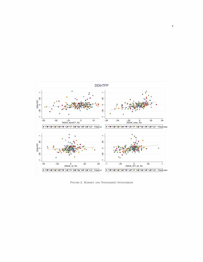
Figure 1 shows data on ∆lnTFP for the whole economy against capital growth of NonICT,

ICT, intangibles and R&D. As the figure shows, there is a somewhat positive correlation.

Figure 2 shows the same variables, but in double differences, which is how we shall

estimate the relation and obtains a similar pattern.

8

-.1-.0

50

.05

Dln

TFP

-.02 0 .02 .04 .06DlnK_NonICT_Tot

“FR” “DE” “SE” “DK” “FI” “UK” “IT” “ES” “NL” “AT” “US” “CZ” Fitted values

-.1-.0

50

.05

-.02 0 .02 .04 .06 .08DlnK_intan_Tot

“FR” “DE” “SE” “DK” “FI” “UK” “IT” “ES” “NL” “AT” “US” “CZ” Fitted values

-.1-.0

50

.05

Dln

TFP

-.05 0 .05 .1DlnK_rd_Tot

“FR” “DE” “SE” “DK” “FI” “UK” “IT” “ES” “NL” “AT” “US” “CZ” Fitted values

-.1-.0

50

.05

0 .05 .1 .15 .2 .25DlnK_ICT_isf_Tot

“FR” “DE” “SE” “DK” “FI” “UK” “IT” “ES” “NL” “AT” “US” “CZ” Fitted values

DlnTFP

Figure 1. Labor productivity growth, whole economy and capital inputs

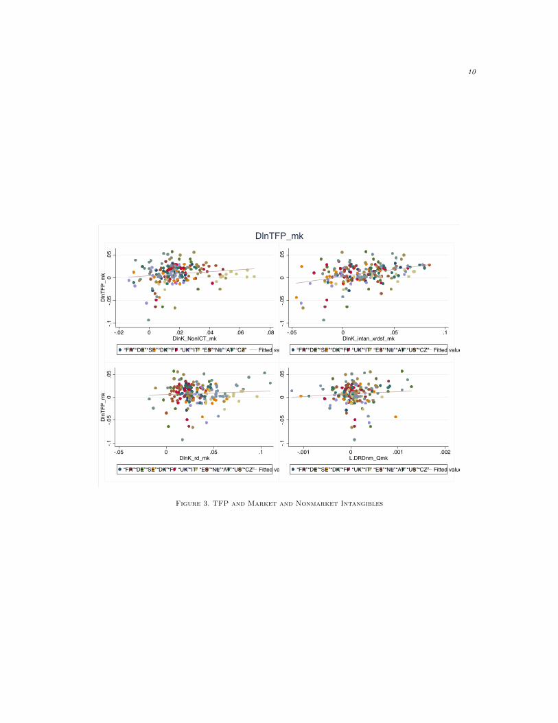
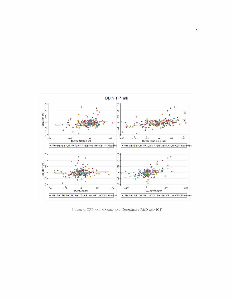
Figure 3 shows not ∆lnTFP for the whole economy, but ∆lnTFP for the market sector.

This is constructed, as above, as a value added weighted sum of ∆lnTFP for each country-

year, summing over the market sector in each of the industries in each country-year. We

have plotted this against (growth in log) nonICT capital in the market sector, intangible

capital excluding R&D, R&D capital, and, in the bottom panel, the (lagged) level of non-

market R&D investment as a proportion of market value added. The final correlation is an

indication of spillovers from the public to the private sector.

Finally, Figure 4 shows the above figure, but in double differences.

9

-.1-.0

50

.05

.1D

Dln

TFP

-.03 -.02 -.01 0 .01DDlnK_NonICT_Tot

“FR” “DE” “SE” “DK” “FI” “UK” “IT” “ES” “NL” “AT” “US” “CZ” Fitted values

-.1-.0

50

.05

.1

-.06 -.04 -.02 0 .02 .04DDlnK_intan_Tot

“FR” “DE” “SE” “DK” “FI” “UK” “IT” “ES” “NL” “AT” “US” “CZ” Fitted values

-.1-.0

50

.05

.1D

Dln

TFP

-.04 -.02 0 .02 .04DDlnK_rd_Tot

“FR” “DE” “SE” “DK” “FI” “UK” “IT” “ES” “NL” “AT” “US” “CZ” Fitted values

-.1-.0

50

.05

.1

-.1 -.05 0 .05 .1DDlnK_ICT_isf_Tot

“FR” “DE” “SE” “DK” “FI” “UK” “IT” “ES” “NL” “AT” “US” “CZ” Fitted values

DDlnTFP

Figure 2. Market and Nonmarket Intangibles

10

-.1-.0

50

.05

Dln

TFP_

mk

-.02 0 .02 .04 .06 .08DlnK_NonICT_mk

“FR” “DE” “SE” “DK” “FI” “UK” “IT” “ES” “NL” “AT” “CZ” Fitted values

-.1-.0

50

.05

-.05 0 .05 .1DlnK_intan_xrdsf_mk

“FR” “DE” “SE” “DK” “FI” “UK” “IT” “ES” “NL” “AT” “US” “CZ” Fitted values

-.1-.0

50

.05

Dln

TFP_

mk

-.05 0 .05 .1DlnK_rd_mk

“FR” “DE” “SE” “DK” “FI” “UK” “IT” “ES” “NL” “AT” “US” “CZ” Fitted values

-.1-.0

50

.05

-.001 0 .001 .002L.DRDnm_Qmk

“FR” “DE” “SE” “DK” “FI” “UK” “IT” “ES” “NL” “AT” “US” “CZ” Fitted values

DlnTFP_mk

Figure 3. TFP and Market and Nonmarket Intangibles

11

-.1-.0

50

.05

.1.1

5D

Dln

TFP_

mk

-.04 -.02 0 .02DDlnK_NonICT_mk

“FR” “DE” “SE” “DK” “FI” “UK” “IT” “ES” “NL” “AT” “CZ” Fitted values

-.1-.0

50

.05

.1.1

5

-.06 -.04 -.02 0 .02 .04DDlnK_intan_xrdsf_mk

“FR” “DE” “SE” “DK” “FI” “UK” “IT” “ES” “NL” “AT” “US” “CZ” Fitted values

-.1-.0

50

.05

.1.1

5D

Dln

TFP_

mk

-.04 -.02 0 .02 .04DDlnK_rd_mk

“FR” “DE” “SE” “DK” “FI” “UK” “IT” “ES” “NL” “AT” “US” “CZ” Fitted values

-.1-.0

50

.05

.1.1

5

-.001 0 .001 .002L.DRDnm_Qmk

“FR” “DE” “SE” “DK” “FI” “UK” “IT” “ES” “NL” “AT” “US” “CZ” Fitted values

DDlnTFP_mk

Figure 4. TFP and Market and Nonmarket R&D and ICT

12

V. The transition to econometric work

To estimate (5) we must take a number of steps. Recall that our raw data is institutional

sector-industry-country-year, where by institutional sector we mean market or non-market.

Consider then the following model for ∆lnTFP in industry i

∆lnTFPQi,c,t = dLi,c,t∆lnLi,c,t + dKi,c,t∆lnKi,c,t + dRi,c,t∆lnRi,c,t(8)

+γi,c,t∆lnR i,c,t

which assumes that industry i can obtain spillovers potentially from L, K and R in it’s own

industry, but the only outside-industry spillovers are via R outside the industry, denoted

R i (that is, tangible capital outside a firm’s industry conveys no spillovers, but intangible

capital does).

Now, as set out by e.g., Griliches, knowledge outside the industry is of potentially very

many dimensions. To reduce it to something estimable is typically done by devising a

measure that weights the various ∆ lnRi in some way e.g., by technological distance, in-

put/output relations etc. Assume this amounts to a weighted sum over industries with

weights ωi,j 6=i, i.e., industry i has a vector of weights on other industries j, we can write

∆lnTFPQi,c,t = dLi,c,t∆lnLi,c,t + dKi,c,t∆lnKi,c,t + dRi,c,t∆lnRi,c,t(9)

+ γi,c,t(Σωi,j 6=i∆lnRi,c,t) .

A. Aggregated data

At the time of writing we do not have detailed data by industry that would allow us to

model ω as industry links with the public sector (i.e., as inter-industry purchases weights,

as previously done in the literature for private R&D). We are in the process of collecting

these data. So for the time being we work with two data sets. The first is a country-

year or “total economy” dataset (it not quite a total economy dataset because we have

dropped agriculture, real estate and some other small industries, see above), where we take

all our industries and institutional sectors and for each country-year compute, as above,

value-added weighted average of changes in the log of each variable. We then estimate for

country c in time t

13

∆ lnTFPQc,t = ac + at + dL∆lnLc,t + dICT∆lnKICTc,t + dNonICT∆lnKNonICT

c,t(10)

+ dR∆lnRc,t + vc,t

where the inter-industry effects collapse into a single effect of R and we have added country

and time effects to control for this element of unobserved heterogeneity and vc,t is an iid

error term.

The interpretation of this equation depends upon what is included in TFP. Recall that R

is capitalised into ∆ lnTFPQ via value added and via inputs that are given a rate of return

when calculating factor shares (with market sector given an ex-post rate of return and

non-market sector a rate of return equal to the social rate of time preference, as previously

mentioned). Thus the dR is an “excess” output elasticity in the sense of excess over that

elasticity implied by the private and social time preference-based rates of return.

Our second approach is to collapse the output and input data into a “market sector”

and “non-market sector.” The “market sector” is an aggregation into more or less a non-

farm business sector, that is, all sectors excluding agriculture, public administration, public

health and public education. In most countries, this aggregation is close to entirely mar-

ket/for profit i.e. there are very few non-market manufacturing firms for example. But it

does of course miss out for-profit education and health. We then construct ∆lnTFP growth

for what we shall call the “market” sector. We look for knowledge spillovers by looking at

correlations with market sector and non-market knowledge as follows

∆lnTFPQ,MKTc,t = ac + at + dL∆lnLMKT

c,t + dK∆lnKMKTc,t + dR∆lnRMKT

c,t(11)

+ ρ(NNonMKT /QMKT )c,t + vc,t

Here we have written the elasticity times the log change in the non-market stock of R in

terms of its flow i.e. γc∆lnRNonMKTc,t = ρ(NNonMKT /QMKT )c,t where NNonMKT is the

flow of investment by the non-market sector in R.4

The interpretation of dR is an “excess over market” returns because output includes R&D

and inputs include market R&D at its ex post user cost. The interpretation of ρ is a spillover

from non-market to market. Thus the use of market aggregation does not give a full account

of inter-industry spillovers but is a first-pass at a summary of spillovers from non-market

knowledge creation to the market sector.

4 Assume that public R&D does not depreciate (to the extent it is “basic” then is likely to at least becomeless obsolete than private R&D; the ONS report using a depreciation rate of 5% for government R&D for example.)From the perpetual inventory model, ∆lnRNonMKT

t = NNonMKT /RNonMKTt−1 when δNonMKT = 0. Thus the

elasticity of market output (∂Q/∂RNonMKT )(RNonMKT /Q) times this term can be written=(ρit)(RPUB/Q) where

ρit = (∂Q/∂RNonMKT ).

14

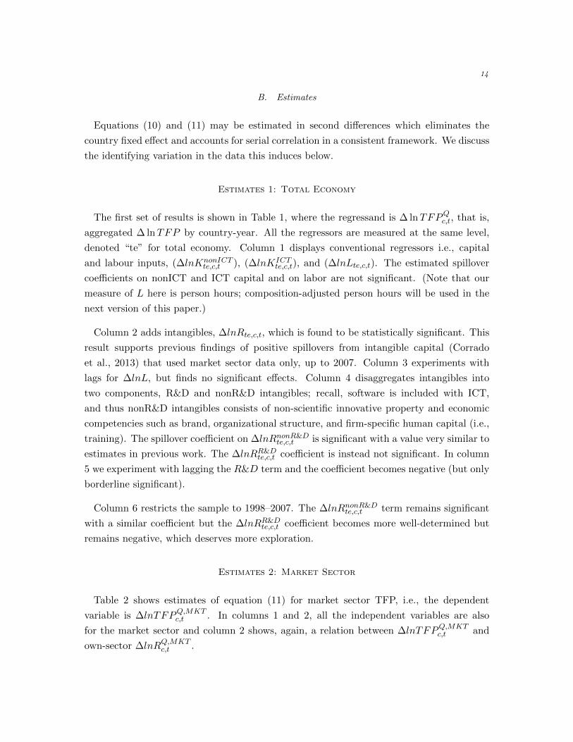
B. Estimates

Equations (10) and (11) may be estimated in second differences which eliminates the

country fixed effect and accounts for serial correlation in a consistent framework. We discuss

the identifying variation in the data this induces below.

Estimates 1: Total Economy

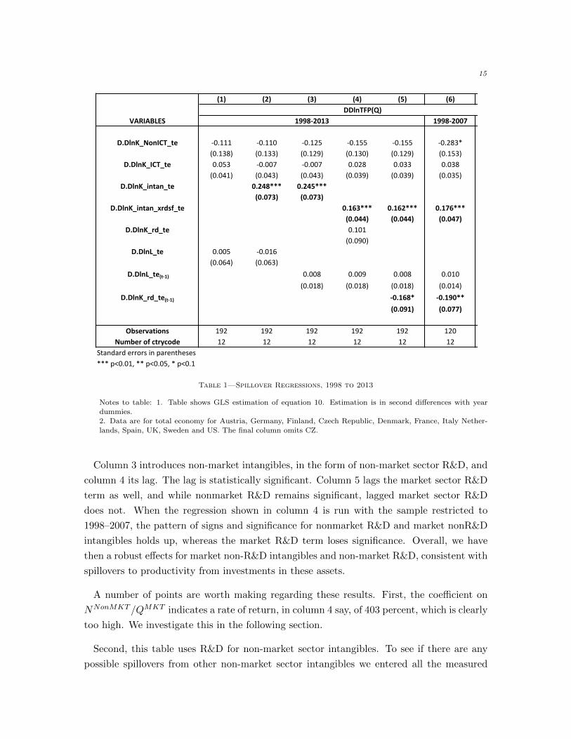
The first set of results is shown in Table 1, where the regressand is ∆ lnTFPQc,t, that is,

aggregated ∆ lnTFP by country-year. All the regressors are measured at the same level,

denoted “te” for total economy. Column 1 displays conventional regressors i.e., capital

and labour inputs, (∆lnKnonICTte,c,t ), (∆lnKICT

te,c,t), and (∆lnLte,c,t). The estimated spillover

coefficients on nonICT and ICT capital and on labor are not significant. (Note that our

measure of L here is person hours; composition-adjusted person hours will be used in the

next version of this paper.)

Column 2 adds intangibles, ∆lnRte,c,t, which is found to be statistically significant. This

result supports previous findings of positive spillovers from intangible capital (Corrado

et al., 2013) that used market sector data only, up to 2007. Column 3 experiments with

lags for ∆lnL, but finds no significant effects. Column 4 disaggregates intangibles into

two components, R&D and nonR&D intangibles; recall, software is included with ICT,

and thus nonR&D intangibles consists of non-scientific innovative property and economic

competencies such as brand, organizational structure, and firm-specific human capital (i.e.,

training). The spillover coefficient on ∆lnRnonR&Dte,c,t is significant with a value very similar to

estimates in previous work. The ∆lnRR&Dte,c,t coefficient is instead not significant. In column

5 we experiment with lagging the R&D term and the coefficient becomes negative (but only

borderline significant).

Column 6 restricts the sample to 1998–2007. The ∆lnRnonR&Dte,c,t term remains significant

with a similar coefficient but the ∆lnRR&Dte,c,t coefficient becomes more well-determined but

remains negative, which deserves more exploration.

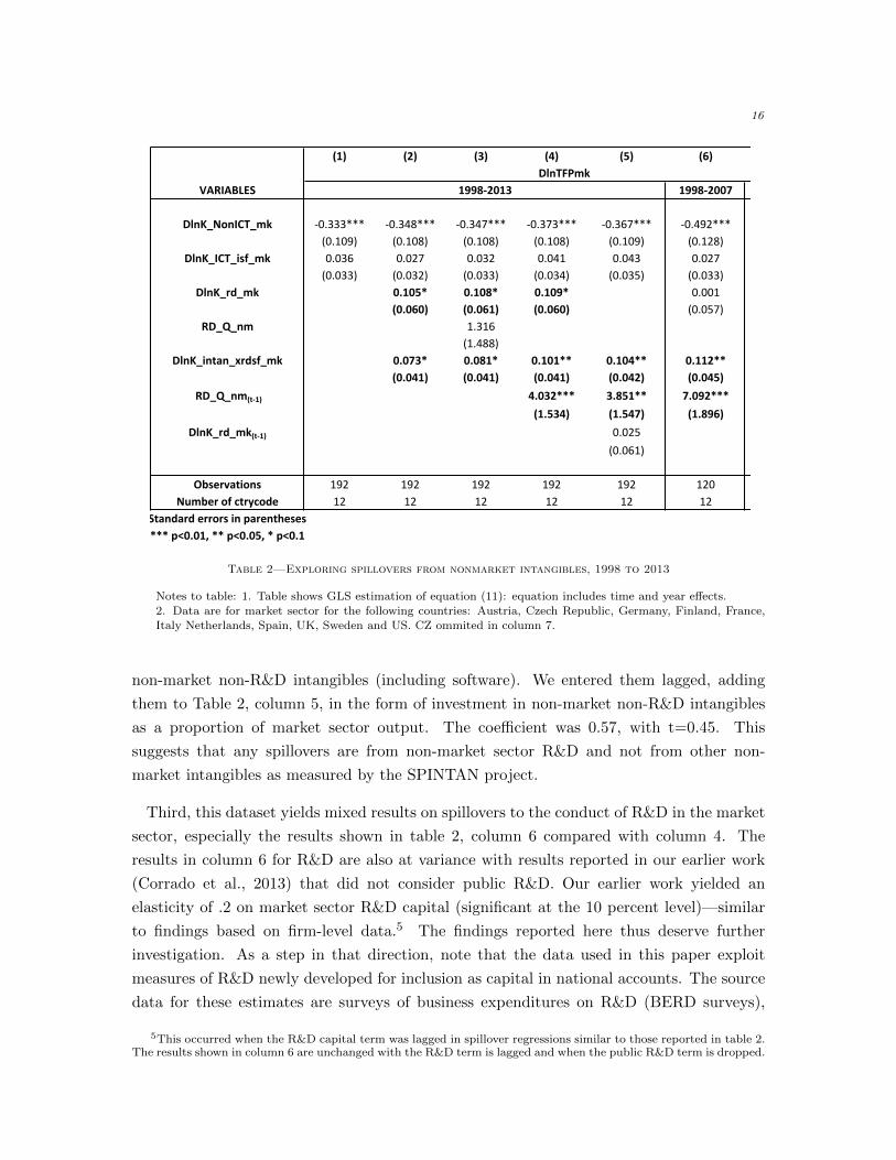
Estimates 2: Market Sector

Table 2 shows estimates of equation (11) for market sector TFP, i.e., the dependent

variable is ∆lnTFPQ,MKTc,t . In columns 1 and 2, all the independent variables are also

for the market sector and column 2 shows, again, a relation between ∆lnTFPQ,MKTc,t and

own-sector ∆lnRQ,MKTc,t .

15

(1) (2) (3) (4) (5) (6) (7)

VARIABLES 1998-2007 exclCZ

D.DlnK_NonICT_te -0.111 -0.110 -0.125 -0.155 -0.155 -0.283* -0.146(0.138) (0.133) (0.129) (0.130) (0.129) (0.153) (0.140)

D.DlnK_ICT_te 0.053 -0.007 -0.007 0.028 0.033 0.038 0.035(0.041) (0.043) (0.043) (0.039) (0.039) (0.035) (0.040)

D.DlnK_intan_te 0.248*** 0.245***

(0.073) (0.073)

D.DlnK_intan_xrdsf_te 0.163*** 0.162*** 0.176*** 0.169***

(0.044) (0.044) (0.047) (0.046)

D.DlnK_rd_te 0.101(0.090)

D.DlnL_te 0.005 -0.016(0.064) (0.063)

D.DlnL_te(t-1) 0.008 0.009 0.008 0.010 0.008(0.018) (0.018) (0.018) (0.014) (0.017)

D.DlnK_rd_te(t-1) -0.168* -0.190** -0.252**

(0.091) (0.077) (0.099)

Observations 192 192 192 192 192 120 176Numberofctrycode 12 12 12 12 12 12 11

Standarderrorsinparentheses***p<0.01,**p<0.05,*p<0.1

DDlnTFP(Q)

1998-2013

Table 1—Spillover Regressions, 1998 to 2013

Notes to table: 1. Table shows GLS estimation of equation 10. Estimation is in second differences with yeardummies.

2. Data are for total economy for Austria, Germany, Finland, Czech Republic, Denmark, France, Italy Nether-

lands, Spain, UK, Sweden and US. The final column omits CZ.

Column 3 introduces non-market intangibles, in the form of non-market sector R&D, and

column 4 its lag. The lag is statistically significant. Column 5 lags the market sector R&D

term as well, and while nonmarket R&D remains significant, lagged market sector R&D

does not. When the regression shown in column 4 is run with the sample restricted to

1998–2007, the pattern of signs and significance for nonmarket R&D and market nonR&D

intangibles holds up, whereas the market R&D term loses significance. Overall, we have

then a robust effects for market non-R&D intangibles and non-market R&D, consistent with

spillovers to productivity from investments in these assets.

A number of points are worth making regarding these results. First, the coefficient on

NNonMKT /QMKT indicates a rate of return, in column 4 say, of 403 percent, which is clearly

too high. We investigate this in the following section.

Second, this table uses R&D for non-market sector intangibles. To see if there are any

possible spillovers from other non-market sector intangibles we entered all the measured

16

(1) (2) (3) (4) (5) (6) (7)

VARIABLES 1998-2007 exclCZ

DlnK_NonICT_mk -0.333*** -0.348*** -0.347*** -0.373*** -0.367*** -0.492*** -0.358***(0.109) (0.108) (0.108) (0.108) (0.109) (0.128) (0.112)

DlnK_ICT_isf_mk 0.036 0.027 0.032 0.041 0.043 0.027 0.013(0.033) (0.032) (0.033) (0.034) (0.035) (0.033) (0.033)

DlnK_rd_mk 0.105* 0.108* 0.109* 0.001 0.156***(0.060) (0.061) (0.060) (0.057) (0.060)

RD_Q_nm 1.316(1.488)

DlnK_intan_xrdsf_mk 0.073* 0.081* 0.101** 0.104** 0.112** 0.075*(0.041) (0.041) (0.041) (0.042) (0.045) (0.042)

RD_Q_nm(t-1) 4.032*** 3.851** 7.092*** 3.351**

(1.534) (1.547) (1.896) (1.511)

DlnK_rd_mk(t-1) 0.025(0.061)

Observations 192 192 192 192 192 120 176Numberofctrycode 12 12 12 12 12 12 11

Standarderrorsinparentheses***p<0.01,**p<0.05,*p<0.1

1998-2013DlnTFPmk

Table 2—Exploring spillovers from nonmarket intangibles, 1998 to 2013

Notes to table: 1. Table shows GLS estimation of equation (11): equation includes time and year effects.

2. Data are for market sector for the following countries: Austria, Czech Republic, Germany, Finland, France,Italy Netherlands, Spain, UK, Sweden and US. CZ ommited in column 7.

non-market non-R&D intangibles (including software). We entered them lagged, adding

them to Table 2, column 5, in the form of investment in non-market non-R&D intangibles

as a proportion of market sector output. The coefficient was 0.57, with t=0.45. This

suggests that any spillovers are from non-market sector R&D and not from other non-

market intangibles as measured by the SPINTAN project.

Third, this dataset yields mixed results on spillovers to the conduct of R&D in the market

sector, especially the results shown in table 2, column 6 compared with column 4. The

results in column 6 for R&D are also at variance with results reported in our earlier work

(Corrado et al., 2013) that did not consider public R&D. Our earlier work yielded an

elasticity of .2 on market sector R&D capital (significant at the 10 percent level)—similar

to findings based on firm-level data.5 The findings reported here thus deserve further

investigation. As a step in that direction, note that the data used in this paper exploit

measures of R&D newly developed for inclusion as capital in national accounts. The source

data for these estimates are surveys of business expenditures on R&D (BERD surveys),

5This occurred when the R&D capital term was lagged in spillover regressions similar to those reported in table 2.The results shown in column 6 are unchanged with the R&D term is lagged and when the public R&D term is dropped.

17

and, as compiled by the OECD, such data were the (literal) basis of the earlier study. For

some countries, the OECD’s BERD data are somewhat at variance with the path of R&D

investment in national accounts, where adjustments for net trade and other accounting

conventions are made. Simple charts of the BERD and national accounts R&D data for

the market sector (industry sectors B-M, excluding L and M72) and for manufacturing

(industry sector B) are shown in the appendix to this paper.

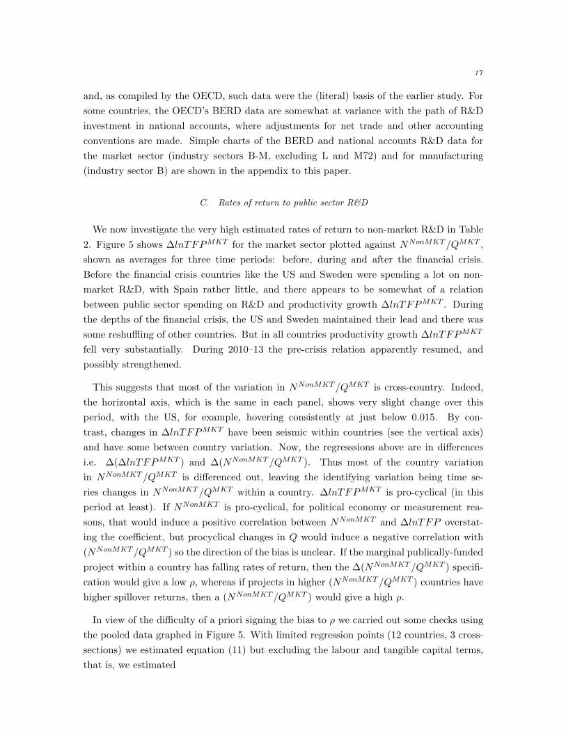
C. Rates of return to public sector R&D

We now investigate the very high estimated rates of return to non-market R&D in Table

2. Figure 5 shows ∆lnTFPMKT for the market sector plotted against NNonMKT /QMKT ,

shown as averages for three time periods: before, during and after the financial crisis.

Before the financial crisis countries like the US and Sweden were spending a lot on non-

market R&D, with Spain rather little, and there appears to be somewhat of a relation

between public sector spending on R&D and productivity growth ∆lnTFPMKT . During

the depths of the financial crisis, the US and Sweden maintained their lead and there was

some reshuffling of other countries. But in all countries productivity growth ∆lnTFPMKT

fell very substantially. During 2010–13 the pre-crisis relation apparently resumed, and

possibly strengthened.

This suggests that most of the variation in NNonMKT /QMKT is cross-country. Indeed,

the horizontal axis, which is the same in each panel, shows very slight change over this

period, with the US, for example, hovering consistently at just below 0.015. By con-

trast, changes in ∆lnTFPMKT have been seismic within countries (see the vertical axis)

and have some between country variation. Now, the regresssions above are in differences

i.e. ∆(∆lnTFPMKT ) and ∆(NNonMKT /QMKT ). Thus most of the country variation

in NNonMKT /QMKT is differenced out, leaving the identifying variation being time se-

ries changes in NNonMKT /QMKT within a country. ∆lnTFPMKT is pro-cyclical (in this

period at least). If NNonMKT is pro-cyclical, for political economy or measurement rea-

sons, that would induce a positive correlation between NNonMKT and ∆lnTFP overstat-

ing the coefficient, but procyclical changes in Q would induce a negative correlation with

(NNonMKT /QMKT ) so the direction of the bias is unclear. If the marginal publically-funded

project within a country has falling rates of return, then the ∆(NNonMKT /QMKT ) specifi-

cation would give a low ρ, whereas if projects in higher (NNonMKT /QMKT ) countries have

higher spillover returns, then a (NNonMKT /QMKT ) would give a high ρ.

In view of the difficulty of a priori signing the bias to ρ we carried out some checks using

the pooled data graphed in Figure 5. With limited regression points (12 countries, 3 cross-

sections) we estimated equation (11) but excluding the labour and tangible capital terms,

that is, we estimated

18

AT

CZ

DEDKES

FI

FR

IT

NL

SE

UK US

AT

CZDE

DK

ES

FI

FR

IT

NL

SE

UK

US

ATCZ

DE

DK

ES

FIFR

ITNL

SE

UK US

0.0

1.0

2.0

3

-.05

-.04

-.03

-.02

-.01

-.01

0.0

1.0

2

0 .005 .01 .015

0 .005 .01 .015

1996-07 2008-09

2010-13

Dln

TFP,

mar

ket s

ecto

r

(Non-market R&D spend)/(market sector value added), laggedGraphs by period

Figure 5. DlnTFP, market sector and Nonmarket R&D

∆lnTFPQ,MKTc,t = ac + at + dK∆lnKMKT

intan,c,t + dR∆lnRMKTc,t(12)

+ ρ(NNonMKT /QMKT )c,t + vc,t

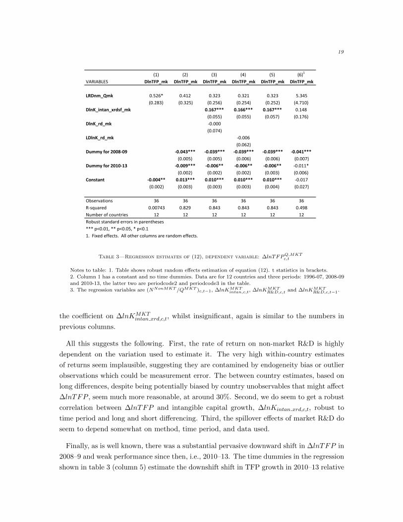
Table 3 shows estimates of equation (12).

Column 1 shows a simple pooled regression corresponding to Figure 5, and suggests

a public rate of return of 53 percent. Column 2 adds period dummies and the return

drops: note too the rise in the R2 showing the considerable common time variation in

∆lnTFPQ,MKTc,t . Column 3 adds market intangibles, with the nonR&D and R&D as sep-

arate regressors. ∆lnKMKTintan xrd,c,t is significant whereas ∆lnKMKT

R&D,c,t is insignificant. The

coefficient on (NNonMKT /QMKT )c,t−1 has fallen further to a return of 32 percent, where it

would appear that some of the cross-country variation in public R&D spending is taken

up by these regressors. Column 4 lags ∆lnKMKTR&D,c,t, which remains insignificant, and

column 5 drops it altogether. Finally, column 6 enters fixed effects. The coefficient on

(NNonMKT /QMKT )c,t−1 rises to 534 percent, echoing the high numbers found above, and

19

(1) (2) (3) (4) (5) (6)1

VARIABLES DlnTFP_mk DlnTFP_mk DlnTFP_mk DlnTFP_mk DlnTFP_mk DlnTFP_mk

LRDnm_Qmk 0.526* 0.412 0.323 0.321 0.323 5.345(0.283) (0.325) (0.256) (0.254) (0.252) (4.710)

DlnK_intan_xrdsf_mk 0.167*** 0.166*** 0.167*** 0.148(0.055) (0.055) (0.057) (0.176)

DlnK_rd_mk -0.000(0.074)

LDlnK_rd_mk -0.006(0.062)

Dummyfor2008-09 -0.043*** -0.039*** -0.039*** -0.039*** -0.041***(0.005) (0.005) (0.006) (0.006) (0.007)

Dummyfor2010-13 -0.009*** -0.006** -0.006** -0.006** -0.011*(0.002) (0.002) (0.002) (0.003) (0.006)

Constant -0.004** 0.013*** 0.010*** 0.010*** 0.010*** -0.017(0.002) (0.003) (0.003) (0.003) (0.004) (0.027)

Observations 36 36 36 36 36 36R-squared 0.00743 0.829 0.843 0.843 0.843 0.498Numberofcountries 12 12 12 12 12 12Robuststandarderrorsinparentheses***p<0.01,**p<0.05,*p<0.11.Fixedeffects.Allothercolumnsarerandomeffects.

Table 3—Regression estimates of (12), dependent variable: ∆lnTFPQ,MKTc,t

Notes to table: 1. Table shows robust random effects estimation of equation (12). t statistics in brackets.2. Column 1 has a constant and no time dummies. Data are for 12 countries and three periods: 1996-07, 2008-09

and 2010-13, the latter two are periodcode2 and periodcode3 in the table.

3. The regression variables are (NNonMKT /QMKT )c,t−1, ∆lnKMKTintan,c,t, ∆lnKMKT

R&D,c,t and ∆lnKMKTR&D,c,t−1.

the coefficient on ∆lnKMKTintan xrd,c,t, whilst insignificant, again is similar to the numbers in

previous columns.

All this suggests the following. First, the rate of return on non-market R&D is highly

dependent on the variation used to estimate it. The very high within-country estimates

of returns seem implausible, suggesting they are contamined by endogeneity bias or outlier

observations which could be measurement error. The between country estimates, based on

long differences, despite being potentially biased by country unobservables that might affect

∆lnTFP , seem much more reasonable, at around 30%. Second, we do seem to get a robust

correlation between ∆lnTFP and intangible capital growth, ∆lnKintan xrd,c,t, robust to

time period and long and short differencing. Third, the spillover effects of market R&D do

seem to depend somewhat on method, time period, and data used.

Finally, as is well known, there was a substantial pervasive downward shift in ∆lnTFP in

2008–9 and weak performance since then, i.e., 2010–13. The time dummies in the regression

shown in table 3 (column 5) estimate the downshift shift in TFP growth in 2010–13 relative

20

to 1999–2003 to be 1.6 percentage points, which is substantial.6 Thus on this model we have

a quite substantial unexplained common decline in ∆lnTFP after the Great Recession. This

much discussed slowdown in productivity growth, as reflected in the data used in this study,

is relative to a rather exceptional period, however. While TFP growth for the countries

in our sample averaged 1.6 percent during 1999–2007 (and .8 percentage points during

2010–13), average TFP growth from 1999 to 2003 masks substantial heterogeneity in the

sample, with US TFP growth relatively strong from 1999 to 2003 and EU growth relatively

strong from 2004 to 2007. In subsequent work, we plan to experiment with weighted pooled

regressions and look at these periods separately.

VI. Conclusions

We have used a new cross-country sector-industry-level (i.e. data for industries and

market/non-market within industries) growth accounting database that includes data on

intangible investment for 11 EU countries (Austria, Czech Republic, Germany, Finland,

France, Italy Netherlands, UK, Sweden) and the United States from 1995 through 2013.

We build tangible and intangible captial stocks from investment data, use harmonised ICT

prices and account for public sector rates of return using the approach of Jorgenson and

Scheyrer. Using R&D investment time series newly developed for national accounts, we

find support for earlier findings in the literature (e.g., Guellec and Van Pottelsberghe de la

Potterie 2002, 2004) that there are spillovers from public sector R&D to market sector

productivity. Our findings suggest a rate of return of around 30% to public sector R&D

spend. We also find that market sector investments in nonR&D intangible capital generate

spillovers to productivity. Finally, we do not find evidence that non-market non-R&D

intangible investment has spillover benefits to the market sector.

REFERENCES

Bacchini et al., F. (2016). Estimates of intangible investment in the public sector: EU, US,

China and Brazil. SPINTAN Working Paper Series 11.

Brynjolfsson, E., L. M. Hitt, and S. Yang (2002). Intangible assets: Computers and orga-

nizational capital. Brookings Papers on Economic Activity 2002:1, 137–198.

Caves, D. W., L. R. Christensen, and W. E. Diewert (1982). The economic theory of index

numbers and the measurement of input, output, and productivity. Econometrica 50 (6),

1393–1414.

6The dummies estimated in table 3 are similar to the shifts in the (unreported) coefficients on time dummies forthe regressions shown in table 2.

21

Corrado, C., J. Haskel, and C. Jona-Lasinio (2013). Knowledge spillovers, ICT, and pro-

ductivity growth. Working paper, The Conference Board, Imperial College, LUISS and

ISTAT.

Corrado, C., J. Haskel, and C. Jona-Lasinio (2016a). ICT, R&D and non-R&D intangible

capital: Complementary relations and industry productivity growth in EU countries. In

D. W. Jorgenson, K. Fukao, and M. Timmer (Eds.), Growth and Stagnation in the World

Economy, pp. 319–346. Cambridge University Press.

Corrado, C., J. Haskel, and C. Jona-Lasinio (2016b). Public intangibles: The public sector

and economic growth in the SNA. Review of Income and Wealth (forthcoming). Available

as SPINTAN Working Paper Series 1.

Corrado, C., J. Haskel, C. Jona-Lasinio, M. Iommi, and M. Mahony (2016). Sources of

country-sector productivity growth: Total factor productivity and intangible capital in

the EU15 and the US. Paper prepared for the 2016 IARIW Conference, Dresden, Ger-

many.

Corrado, C. and C. Hulten (2010). How do you measure a ‘Technological Revolution’? The

American Economic Review 100 (2, May), 99–104.

Corrado, C., C. Hulten, and D. Sichel (2005). Measuring capital and technology: An

expanded framework. In C. Corrado, J. Haltiwanger, and D. Sichel (Eds.), Measuring

Capital in the New Economy, Studies in Income and Wealth No. 65, pp. 11–46. Chicago:

University of Chicago Press.

Corrado, C., C. Hulten, and D. Sichel (2009). Intangible capital and U.S. economic growth.

Review of Income and Wealth 55 (3), 661–685.

Corrado, C. and K. Jager (2015). The social rate of time preference as the return on public

assets. SPINTAN Deliverable D1.6, The Conference Board.

Eberhardt, M., C. Helmers, and H. Strauss (2013). Do spillovers matter when estimating

private returns to R&D? Review of Economics and Statistics 95 (2), 436–448.

Feldstein, M. (1964). The social rate of time preference discount rate in cost benefit analysis.

The Economic Journal 74 (294), 360–379.

Griliches, Z. (1979). Issues in assessing the contribution of research and development to

productivity growth. Bell Journal of Economics 10 (1), 92–119.

Griliches, Z. (1992). The search for R&D spillovers. Scandinavian Journal of Eco-

nomics 94 (Supplement), S29–47.

22

Guellec, D. and B. Van Pottelsberghe de la Potterie (2002). R&D and productivity growth

a panel data analysis of 16 OECD countries. OECD Economic Studies 33, 103–126.

Guellec, D. and B. Van Pottelsberghe de la Potterie (2004). From R&D to productivity

growth: Do the institutional settings and the source of funds of R&D matter? Oxford

Bulletin of Economics and Statistics 66 (3), 353–378.

Hall, B. H., J. Mairesse, and P. Mohnen (2009). Measuring the returns to R&D. NBER

working paper 15622, NBER Working Paper 15622.

Harper, M., B. P. Moulton, S. Rosenthal, and D. B. Wasshausen (2009). Integrated GDP–

productivity accounts. American Economic Review 99 (2), 74–78.

Inklaar, R., M. P. Timmer, and B. van Ark (2008). Market services productivity across

Europe and the US. Economic Policy 23 (53), 139–194.

Iommi, M., C. Corrado, J. Haskel, and C. Jona-Lasinio (2016). [EIB Paper]. Technical

report.

Jorgenson, D. W. and Z. Griliches (1967). The explanation of productivity change. The

Review of Economic Studies 34 (3), 249–283.

Jorgenson, D. W. and J. S. Landefeld (2006). Blueprint for expanded and integrated U.S.

accounts: Review, assessment, and next steps. In D. W. Jorgenson, J. S. Landefeld, and

W. D. Nordhaus (Eds.), A New Architecture for the U.S. National Accounts, Volume 66

of NBER Studies in Income and Wealth, pp. 13–112. Chicago: University of Chicago

Press. Available at http://www.nber.org/chapters/c0133.pdf.

Krueger, A. B. and M. Lindahl (2001). Education for growth: Why and for whom? Journal

of Economic Literature 39 (4), pp. 1101–1136.

Moretti, E. (2004a). Estimating the social return to higher education: evidence from lon-

gitudinal and repeated cross-sectional data. Journal of Econometrics 121 (1), 175–212.

Moretti, E. (2004b). Workers education, spillovers, and productivity: Evidence from plant-

level production functions. The American Economic Review 94 (3), 656–690.

Solow, R. M. (1957). Technical change and the aggregate production function. The Review

of Economics and Statistics 39 (3), 312–320.

Stiroh, K. J. (2002). Are ICT spillovers driving the new economy? Review of Income and

Wealth 48 (1), 33–57.

23

234567

1995

2000

2005

2010

2015

NA

BERD_ISIC4

BERD_ISIC31AT

10203040

1995

2000

2005

2010

2015

NA

BERD_ISIC4

BERD_ISIC31CZ

30405060

1995

2000

2005

2010

2015

NA

BERD_ISIC4

BERD_ISIC31DE

1020304050

1995

2000

2005

2010

2015

NA

BERD_ISIC4

BERD_ISIC31DK

24681012

1995

2000

2005

2010

2015

NA

BERD_ISIC4

BERD_ISIC31ES

123456

1995

2000

2005

2010

2015

NA

BERD_ISIC4

BERD_ISIC31FI

1020304050

1995

2000

2005

2010

2015

NA

BERD_ISIC4

BERD_ISIC31FR

468101214

1995

2000

2005

2010

2015

NA

BERD_ISIC4

BERD_ISIC31IT

246810

1995

2000

2005

2010

2015

NA

BERD_ISIC4

BERD_ISIC31NL

406080100120

1995

2000

2005

2010

2015

NA

BERD_ISIC4

BERD_ISIC31SE

0510152025

1995

2000

2005

2010

2015

NA

BERD_ISIC4

BERD_ISIC31UK

100150200250300350

1995

2000

2005

2010

2015

NA

BERD_ISIC4

BERD_ISIC31US

Figure1.BERD

and

NationalAccountsR&D

data

Note

.B

ER

Dd

ata

dow

nlo

ad

edfr

om

OE

CD

web

site

Ju

ly14,

2016.

Nati

on

al

acc

ou

nts

data

are

sou

rced

from

EU

RO

-

ST

AT

;p

roce

ssed

into

SP

INT

AN

data

base

Ju

ly18,

2016.

24

12345

1995

2000

2005

2010

2015

NA

BERD_ISIC4

BERD_ISIC31AT

51015202530

1995

2000

2005

2010

2015

NA

BERD_ISIC4

BERD_ISIC31CZ

2530354045

1995

2000

2005

2010

2015

NA

BERD_ISIC4

BERD_ISIC31DE

51015202530

1995

2000

2005

2010

2015

NA

BERD_ISIC4

BERD_ISIC31DK

12345

1995

2000

2005

2010

2015

NA

BERD_ISIC4

BERD_ISIC31ES

12345

1995

2000

2005

2010

2015

NA

BERD_ISIC4

BERD_ISIC31FI

10152025

1995

2000

2005

2010

2015

NA

BERD_ISIC4

BERD_ISIC31FR

456789

1995

2000

2005

2010

2015

NA

BERD_ISIC4

BERD_ISIC31IT

2.533.544.5

1995

2000

2005

2010

2015

NA

BERD_ISIC4

BERD_ISIC31NL

405060708090

1995

2000

2005

2010

2015

NA

BERD_ISIC4

BERD_ISIC31SE

0246810

1995

2000

2005

2010

2015

NA

BERD_ISIC4

BERD_ISIC31UK

50100150200250

1995

2000

2005

2010

2015

NA

BERD_ISIC4

BERD_ISIC31US

Figure2.BERD

and

NationalAccountsManufa

cturing

R&D

data

Note

.B

ER

Ddata

dow

nlo

ad

edfr

om

OE

CD

web

site

Ju

ly14,

2016.

Nati

on

al

acc

ou

nts

data

are

sou

rced

from

EU

RO

-

ST

AT

;p

roce

ssed

into

SP

INT

AN

data

base

Ju

ly18,

2016.