Spectral Distribution and Density Functions

• We started with the basic model Xt = Rcos(ωt) + εt

where ω is the ’dominant’ frequency; f = ω/2π is the

number of cycles per unit of time and λ = 2π/ω is the

’dominant’ wavelength or period.

• This model can be generalized to

Xt =k∑

j=1

Rj cos(ωjt + φj) + εt

which considers the existence of k-relevant frequencies

ω1, ω2, . . . , ωk.

• Given the trigonometric identity

218

cos(x + y) = cos(x)cos(y) − sin(x)sin(y), we have that

Xt =k∑

j=1

(aj cos(ωjt) + bj sin(ωjt)) + εt

with aj = Rjcos(φj) and bj = −Rjsin(φj).

• By making k → ∞, it can be shown that

Xt =

∫ π

0cos(ωt)du(ω) +

∫ π

0sin(ωt)dv(ω)

where u(ω) and v(ω) are continuous stochastic processes.

This is the spectral representation of Xt.

• The Wiener-Khintchine Theorem says that if γ(k) is the

autocovariance function of Xt, there must exist a

219

monotonically increasing function F (ω) such that

γ(k) =

∫ π

0cos(ωk)dF (ω)

• The function F (ω) is the spectral distribution function of

the process Xt.

• Notice that for k = 0,

γ(0) =

∫ π

0dF (ω) = F (π) = σ2

x

so all other variation in the process is for 0 < ω < π.

• We can redefine the spectral distribution function as:

F ∗(ω) = F (ω)/σ2x

and so F ∗(ω) is the proportion of variance accounted by

ω.

220

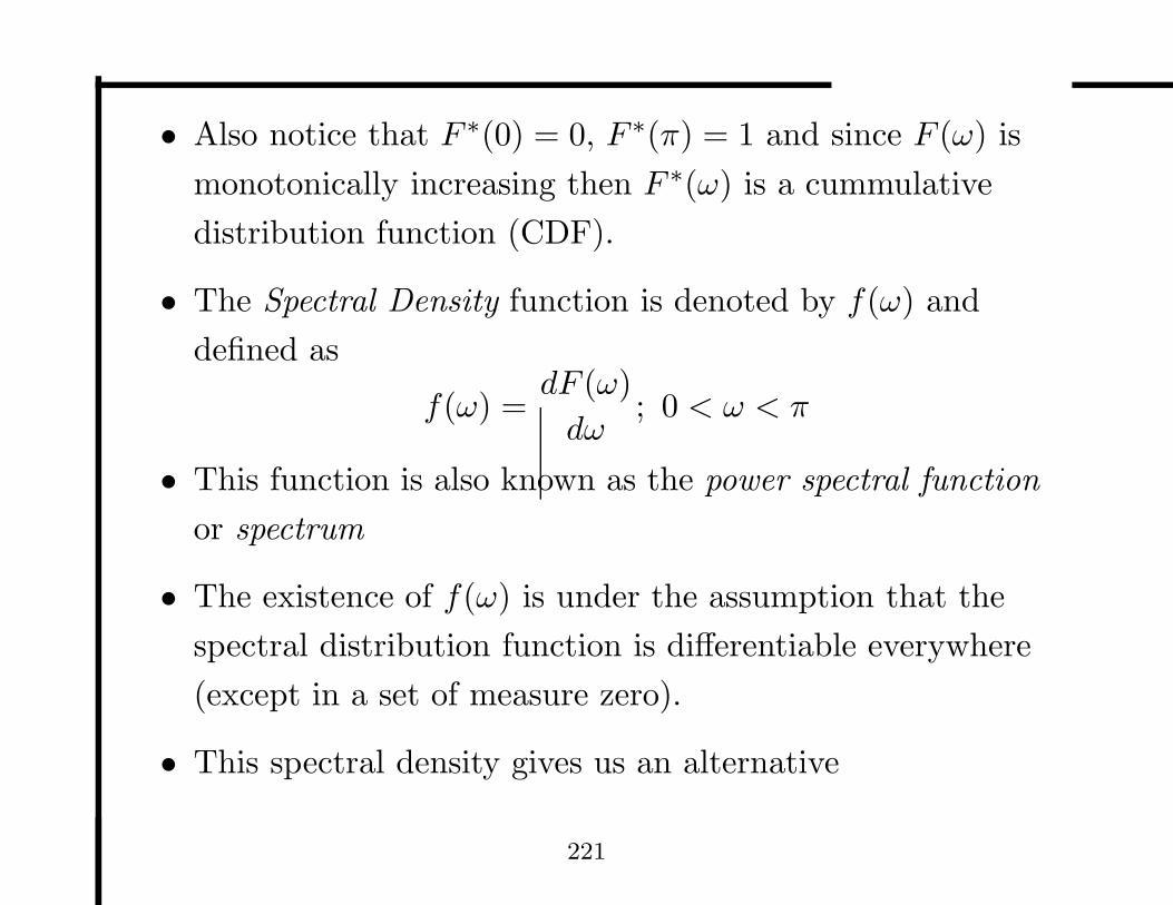
• Also notice that F ∗(0) = 0, F ∗(π) = 1 and since F (ω) is

monotonically increasing then F ∗(ω) is a cummulative

distribution function (CDF).

• The Spectral Density function is denoted by f(ω) and

defined as

f(ω) =dF (ω)

dω; 0 < ω < π

• This function is also known as the power spectral function

or spectrum

• The existence of f(ω) is under the assumption that the

spectral distribution function is differentiable everywhere

(except in a set of measure zero).

• This spectral density gives us an alternative

221

representation for the covariance function

γ(k) =

∫ π

0cos(ωk)f(ω)dω

This characterization is also known as Wold’s Theorem.

• If the spectrum has a ’peak’ at ω0, this implies that ω0 is

an important frequency of the process Xt.

• The spectrum or spectral density is a theoretical function

of the process Xt . In practice, the spectrum is usually

unknown and we use the periodogram to estimate it.

• There is an inverse relationship between the f(ω) and

γ(k),

f(ω) =1

π

∞∑

k=−∞

γ(k)e−iωk

222

so the spectrum is the Fourier transformation of the

autocovariance function.

• From complex analysis, recall that

e−iωk = cos(ωk) − sin(ωk)i

• This implies that

f(ω) =1

π

[

γ(0) + 2∞∑

k=1

γ(k)cos(ωk)

]

• The normalized spectral density f ∗(ω) is defined as:

f∗(ω) =f(ω)

σ2x

=dF ∗(ω)

dω

223

• Then,

f∗(ω) =1

π

[

1 + 2∞∑

k=1

ρ(k)cos(ωk)

]

so the normalized spectrum is the Fourier transform of

the autocorrelation function (ACF).

• Example 1: White noise process. Suppose that Xt is a

purely random process where E(Xt) = 0 and

V ar(Xt) = σ2. The autocovariance function is γ(0) = σ2

and γ(k) = 0; k 6= 0. Thus, the spectral density function

is given by

f(ω) = σ2/π

• Example 2: Consider a first order autoregressive (AR)

process

Xt = αXt−1 + εt; εt ∼ N(0, σ2)

224

The autocovariance function of this process is given by

γ(k) =σ2α|k|

(1 − α2)= σ2

xα|k|; k = 0,±1,±2, . . .

Then, the spectral density function is given by

f(ω) =σ2

π

(

1 +∞∑

k=1

αke−ikω +∞∑

k=1

αeikω

)

after some algebra, this gives

f(ω) = σ2z/[π(1 − 2αcos(ω) + α2)]

• Example 3: Define the sequence Xt by

Xt = A cos(θt) + B sin(θt) + εt

where εt is white noise sequence with variance σ2, A and

225

B are independent random variables with mean zero and

variance τ 2. It can be shown that

E(Xt) = 0;V ar(Xt) = τ2 + σ2

Also, for t 6= s

cov(Xt,Xs) = τ2cos{θ(t − s)}

Then Xt is a stationary series with autocovariance

γ(k) =

{

σ2 + τ2, k = 0

τ2cos(kθ), k 6= 0

The spectrum can be evaluated as

f(ω) = σ2 + τ2 + 2τ2

∞∑

k=1

cos(kθ)cos(kω)

226

= σ2 + τ2 + 2τ2

∞∑

k=1

[cos{k(θ + ω)} + cos{k(θ − ω)}]

If θ = ω, then cos{k(θ − ω)} = 1 for all k and the

summation is infinite.

This means that the spectrum has a ’spike’ at ω = θ.

The spectrum can only exist if we allow f(ω) = ∞ at

isolated values of ω.

227

Periodogram revisited

• For 0 < ω < π, the periodogram is defined as

I(ω) =n

2(a2 + b2)

=2

n

(

n∑

t=1

xtcos(ωt)

)2

+

(

n∑

t=1

xtsin(ωt)

)2

• If ω = 2πj/n; j < n/2 is a Fourier frequency and since∑

t cos(ωt) =∑

t sin(ωt) = 0 then

I(ω) =2

n

(

n∑

t=1

(xt − x)cos(ωt)

)2

+

(

n∑

t=1

(xt − x)sin(ωt)

)2

• Expanding each square term and by the trigonometric

228

identities

(n

2

)

I(ω) =n∑

t=1

(xt − x)2 + 2n−1∑

k=1

n∑

t=k+1

(xt − x)(xt−k − x)cos(ωk)

• This gives an alternative expression for the periodogram,

I(ω) = 2

(

g0 + 2n−1∑

k=1

gkcos(ωk)

)

• We also have a normalized periodogram

I∗(ω) =I(ω)

g0= 2

(

1 + 2n−1∑

k=1

ρkcos(ωk)

)

; ρk = gk/g0

• The last two expressions justify the used of the

periodogram as an estimate of the spectral density.

• What is the sampling distribution of I(ω) ?

229

• By definition, the periodogram satisfies the relation:

nI(ω) = A(ω)2 + B(ω)2

where

A(ω) =n∑

i=1

xtcos(ωt);B(ω) =n∑

i=1

xtsin(ωt)

• To understand the sampling distribution of the

periodogram, lets suppose xt is a realization of a white

noise process (i.i.d. Xt ∼ N(0, σ2)).

• What is the distribution of A(ω) and B(ω)?

• Linear combinations of normal variables are normal.

• In fact, E(A(ω)) = E(B(ω)) = 0

230

• Additionally, by the trigonometric identities,

V ar(A(ω)) = σ2n∑

t=1

cos2(ωt) = (nσ2)/2

V ar(B(ω)) = σ2n∑

t=1

sin2(ωt) = (nσ2)/2

• Also,

Cov(A(ω), B(ω)) = E

[

n∑

t=1

n∑

s=1

XtXscos(ωt)sin(ωs)

]

= σ2n∑

t=1

cos(ωt)sin(ωt) = 0

• It follows that A(ω)√

2/nσ2 and A(ω)√

2/nσ2 are

independent Normal random variables.

231

• Therefore,

2[{A(ω)}2 + {B(ω)}2]/(nσ2) ∼ χ22

• so 2I(ω)/σ2 is a chi-square distribution with 2 degrees of

freedom or

I(ω) ∼ σ2χ22/2

• In particular,

E(I(ω)) = σ2

V (I(ω)) = σ4

• Recall that if Xt is white noise, the spectrum f(ω) = σ2

so in this case I(ω) is unbiased but an inconsistent

estimator of f(ω)

• In fact there is a theorem presented in Diggle’s book

232

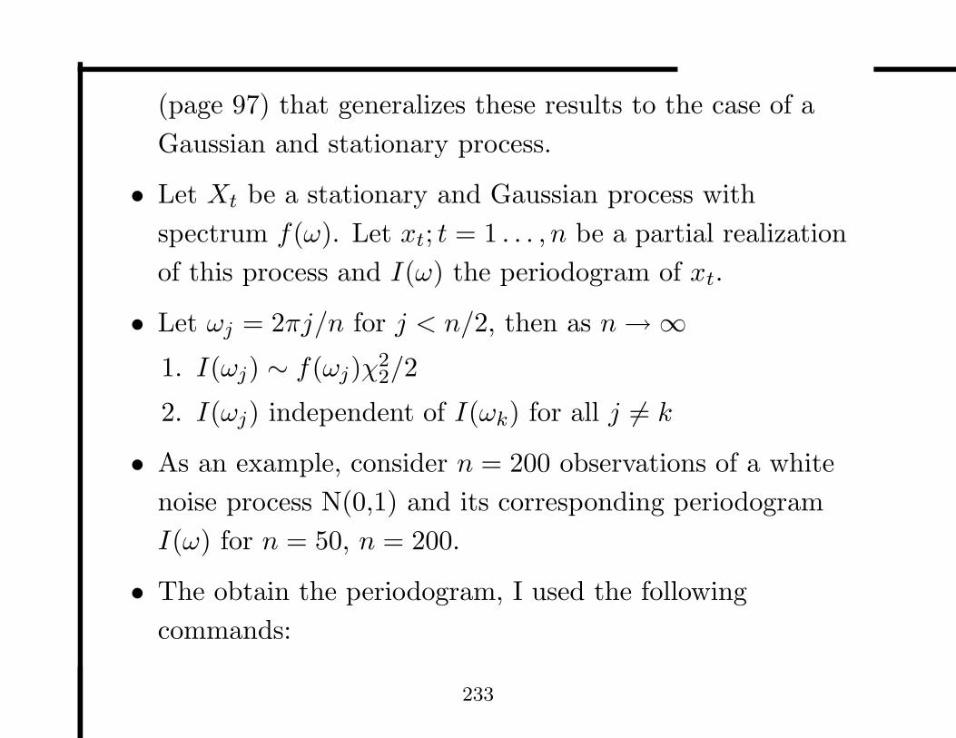
(page 97) that generalizes these results to the case of a

Gaussian and stationary process.

• Let Xt be a stationary and Gaussian process with

spectrum f(ω). Let xt; t = 1 . . . , n be a partial realization

of this process and I(ω) the periodogram of xt.

• Let ωj = 2πj/n for j < n/2, then as n → ∞

1. I(ωj) ∼ f(ωj)χ22/2

2. I(ωj) independent of I(ωk) for all j 6= k

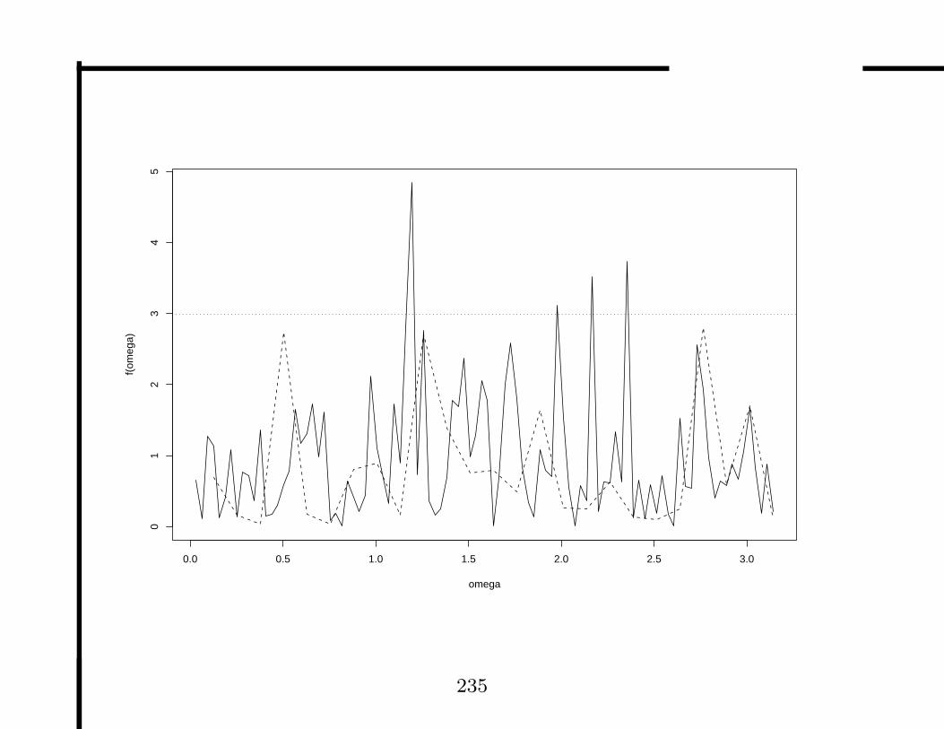
• As an example, consider n = 200 observations of a white

noise process N(0,1) and its corresponding periodogram

I(ω) for n = 50, n = 200.

• The obtain the periodogram, I used the following

commands:

233

x <- rnorm(200)

per <- spec.pgram(x,plot=FALSE)

plot(2*pi*per$freq,per$spec,type=’l’,

xlab="omega",ylab="f(omega)")

per <- spec.pgram(x[1:50],plot=FALSE)

lines(2*pi*per$freq,per$spec,lty=2)

abline(h=qchisq(0.95,2)/2,lty=3)

234

0.0 0.5 1.0 1.5 2.0 2.5 3.0

01

23

45

omega

f(om

ega)

235

• The solid line is the periodogram for all 200 observations

and the dashed line is the periodogram only for the first

50 observations.

• The horizontal line is the .95% quantile of χ22/2 random

variable.

• Notice that variability for the periodogram based on 50

obsevations is similar to the periodogram obtained with

all 200 observations.

• Only a few values of I(ω) are greater than the 0.95

quantile. These values are scattered through the

frequency range.

• The quantile value gives a valid test of significance of the

χ22/2 distribution for a prespecified value of ω.

236

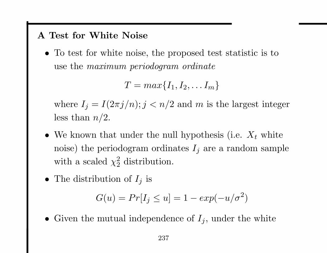
A Test for White Noise

• To test for white noise, the proposed test statistic is to

use the maximum periodogram ordinate

T = max{I1, I2, . . . Im}

where Ij = I(2πj/n); j < n/2 and m is the largest integer

less than n/2.

• We known that under the null hypothesis (i.e. Xt white

noise) the periodogram ordinates Ij are a random sample

with a scaled χ22 distribution.

• The distribution of Ij is

G(u) = Pr[Ij ≤ u] = 1 − exp(−u/σ2)

• Given the mutual independence of Ij , under the white

237

noise hypothesis, the distribution function for T is:

H(t) = G(t)m = (1 − exp(−u/σ2))m

• In practice, usually σ2 is unknown. We can substitute

and estimaor of the variance in H(t) ,

s2 =∑

(xi − x)2/(n − 1), to obtain an approximate test.

• Fisher(1929) deduced the exact distribution for

T0 = T/{∑m

i=1 Ij/m} under a white noise process:

Pr[T0 > mx] =r∑

k=1

[m!/k!(m − r)!](−1)k−1(1 − kx)m−1

where r is the largest integer less than x−1.

• Example For n = 200 observations following a N(0, 1)

distribution, I obtained a value of t = 5.867294 and

238

s2 = 1.037762

1. For the approximate test, the p-value is 0.296048.

2. For Fisher’s test, t0 = 5.619912 and the p-value is

0.2907733

x <- rnorm(200)

I <- spec.pgram(x,plot=F)$spec

t <- max(I)

t0 <- max(I)/mean(I)

s2 <- var(x)

m <- length(I)

1-(1-exp(-t/s2))^m

# k!=gamma(k+1)

239

Tapering

• This is an option that is available within this function

spec.pgram.

spec.pgram(x,taper=0.2)

• A data taper is a transformation of xt into a new series

by multiplying it by constants and to reduce the effect of

extreme observations,

yt = ctxt; t = 1, 2, . . . n

• The sequence ct is chosen to be close to zero at the end

sections of the series, but close to one towards the central

part. (0 < ct ≤ 1).

• If p is the proportion of observations to be tapered, n is

240

total number of observations and m = np, the split cosine

bell taper is defined as :

ct =

.5(1 − cos(π(t − .5)/m)) t = 1, . . . ,m

1 t = m + 1, . . . , n − m

.5(1 − cos(π(n − t − .5)/m)) t = n − m + 1, . . . , n

Smoothing the Periodogram

• If we have the spectrum f(ω) is a smooth function of ω,

another periodogram based estimator of f(ω) is:

f(ωj) = (2p + 1)−1p∑

l=−p

I(ωj+l)

• f(ω) is a simple moving average of I(ω)

241

• If Xt is a stationary random process with spectrum f(ω)

for any Fourier frequency ωj as n → ∞

– f(ωj) ∼ f(ωj)χ22(2p+1)/(2(2p + 1))

– f(ωj) is independent of f(ωk) whenever j − k ≥ 2p + 1

• A general version of this estimator is defined as

f(ωj) =p∑

l=−p

wlI(ωj+l)

with∑p

l=−p wl = 1.

• The asymptotic distribution of f(ω) is given by

f(ω) ∼ f(ω)χ2ν/ν

but now the degrees of freedom are defined as

242

ν = 2/∑p

i=−p w2l

• Now recall that the periodogram can be expressed as

I(ω) = g0 + 2n−1∑

k=1

gkcos(kω)

• A possible explanation of why I(ω) is not such a great

estimator of the spectrum is because gk can be large

when rk ≡ 0, particularly for high values of k.

• As we showed before, the variability of I(ω) is not a

function of the number of data points.

• Alternatively, we could use a truncated Periodogram

243

defined as

IK(ω) = g0 + 2K∑

k=1

gkcos(kω)

for a value of K that is less than n − 1.

• We also have a Lag window Periodogram,

fλ(ω) = g0 + 2n−1∑

k=1

λkgkcos(kω)

where λk is a sequence of constants that needs to be

specified by the user.

• Bartlett (1950) proposed that

244

λk =

1 − k/S k ≤ S

0 k > S

• Daniell (1946) proposed a sequence which corresponds to

the “spans” option of spec.pgram in R/Splus.

λk = sin(πk/S)/(πk/S)

• Parzen (1961) proposed that

λk =

1 − 6(k/S)2 + 6(k/S)3 k ≤ S/2

2(1 − k/S)3 S/2 < k ≤ S

0 k > S

where large values of S correspond to less smoothing.

245

• We consider again the CO2 data and we will look into

different versions of the periodogram. Here is the R code.

data(co2)

co2diff <- as.vector(diff(co2))

par(mfrow=c(2,2))

per<-spec.pgram(co2diff,taper=0,pad=0,detrend=F,

demean=F,plot=F)

lam<-1/per$freq

plam<-per$spec

i<-2<lam & lam<16

plot(lam[i],plam[i],type=’l’,ylab=’periodogram’)

mtext("Raw periodogram")

246

per<-spec.pgram(co2diff,spans=c(6),taper=0,pad=0,

detrend=F,demean=F,plot=F)

per<-spec.pgram(co2diff,taper=0.3,pad=0,detrend=F,

demean=F,plot=F)

per<-spec.pgram(co2diff,spans=c(6),taper=0.2,pad=0,

detrend=F,demean=F,plot=F)

247

2 4 6 8 10 12 14 16

050

100

150

200

lam[i]

perio

dogr

am

Raw periodogram

2 4 6 8 10 12 14 16

010

2030

40

lam[i]

perio

dogr

am

smoothed

2 4 6 8 10 12 14 16

050

100

150

lam[i]

perio

dogr

am

tapered with 0.2

2 4 6 8 10 12 14 16

010

2030

40

lam[i]

perio

dogr

am

smoothed and tapered

248