Embed Size (px)
Citation preview

103
CHAPTER – 4
PROPOSED ALGORITHMS
The work in this chapter is an attempt to propose the techniques
on Non parametric spectrum estimation problems and is reported in
the following sections.
4.1 Need for new algorithms:
Though the non parametric spectral estimation has good dynamic
performance, it has few a drawbacks such as spectral leakage effects
due to windowing, requires long data sequences to obtain the
necessary frequency resolution, assumption of auto correlation
estimate for the lags greater than the length of the sequences to be
zero which limits the quality of the power spectrum and the
assumption of available data are periodic with period N which may not
be realistic. Hence alternatives must be explored to reduce the
spectral leakage effects, to decease the uncertainty in the low
frequency regions, to improve the frequency resolution, to reduce
variance with the increased percentage of overlapping data samples a
consistent spectral estimate with minimum amount of bias and
variance.
The study of spectral leakage effects methods have been discussed
by many authors. In this work, a non parametric power spectrum
estimation method for nonuniform data based on interpolation and
cubicspline interpolation methods is proposed. The simulation results

104
show the reduction in spectral leakage, improved spectral estimation
accuracy and shifting of frequency peaks towards the low frequency
region. The simulation results present a good argument with the
published work.
To reduce the spectral leakage effects and to resolve the spectral
peaks at higher frequencies of non uniform data sequences, a
nonparametric power spectrum estimation method using prewhitening
and post coloring technique is proposed. The combination of
nonparametric with parametric method as preprocessor is proposed in
large active range situations. The simulation results present a good
argument with the published work.
To reduce the variance of a spectral estimate, a non parametric
spectral estimation method based on circular overlapping of samples
is proposed. The existing Welch nonparametric power spectrum
estimation method has increased variance with the increased
percentage of overlapping of samples. Welch estimate uses the linear
overlapping of the samples. Hence the Welch estimate is not a
consistent spectral estimate. To overcome this, circular overlapping of
samples is proposed. The variance of the proposed estimate decreases
with increased percentage of circular overlapping of samples, the
spectral variance is found to be nonmonotonically decreasing
function. The simulation results show the robustness of proposed
estimate with the existing Welch estimate in the published work.

105
The following algorithms are considered to increase the large active
range in spectral estimation, to increase the frequency resolution and
to decrease the variance and these are as follows.
Power Spectrum Estimation of nonuniform data sequences
using nonlinear overlapping of samples.
Power spectrum estimation of nonuniform data sequences in
wide dynamic range using prewhitening and postcoloring
technique.
Power spectrum estimation of nonuniform data sequences using
resampling methods like spline, cubicspline interpolation
techniques and averaged weighted least squares algorithm.
4.2 Power Spectrum Estimation of nonuniform data sequences
using nonlinear overlapping of interpolated samples.
4.2.1 Introduction: The Power spectrum estimation of randomly
spaced samples using nonparametric methods is well known and is
reconsidered in this algorithm. Commonly used nonparametric
methods are Periodogram, Modified Periodogram and Welch methods.
The Periodogram and Modified Periodograms are asymptotically
inconsistent spectral estimators for non uniform samples.
Interpolation techniques (58) like cubicspline and linear interpolations
are employed to convert the nonuniform samples to uniformly
distributed samples and then the estimate is evaluated using the
nonlinear overlapping of samples. Welch method is a consistent
estimate for the random samples and the method is reconsidered for

106
achieving very low variances using different percentage of nonlinear
overlapping of the samples than the existing Bartlett’s method of
estimation. Even though the nonlinear overlapping of samples
produces an amount of discontinuity on the random process; it is
observed that for a Gaussian distributed ergodic wide sense stationary
(WSS) random process the spectrum estimate of power is
asymptotically unbiased. The variance of the proposed estimate
decreases due to nonlinear overlapping of the samples.
4.2.2 Spectral Analysis with Nonlinear Overlaps:
The variance of power spectrum estimation is decreased by
considering the average of the spectrum estimate. In Bartlett’s Method
the entire data length N is divided into K number of segments, with
each segment having the length L=N/K. The Periodograms are
evaluated for each segment and then taking the average of K
periodograms. The average of the resulting estimated power
spectra is taken as the estimated power spectrum. Here the
variance is reduced by a factor K, but a price in spectral resolution is
paid. The Welch Method, [15], eliminates the trade off between
spectral resolution and variance in the Bartlett Method by allowing
the segments to overlap. Furthermore, the truncation window can
also vary. Essentially, the Modified Periodogram Method is applied to
each of the overlapping segments and averaged out. However, the
Welch estimator only uses regular overlap at the signal x (n) with
n=0,1,2, ,…, N-1 is a wide sense stationary Gaussian process. We
divide the signal x(n) in K independent segments such that every

107
segment has length L = N/K. Further, we extract different nonlinear
overlapping sub-records. The i-th overlapping sub-record of the signal
x (n) satisfies,
N)1i)(r1(Lnx)n(x i (4.1)
With 1r0 the fraction of overlap, n=0,…,L-1 and where
N)1i)(rI(Ln denotes )1i)(r1(Ln( ) modulo N imposing
circular overlap. The important property of nonlinear overlap is that
every time sample is an equal number of times member of a sub
record, further the different sub records need to overlap an integer
number of time samples. One can show that the two properties are
respectively satisfied if
m11
Lv1r (4.2)
Where m and v are the integer number of time samples also m N and
v N.
The discrete Fourier transform of the i-th sub-record )(nx ias
)1i)(r1(k2j1L
0n
L/kn2jii e.e)n(x)k(X
(4.3)
We made that all initial phases of the sub records same. In the
beginning of the section, we assumed the signal x(n) to be ergodic and
weakly stationary. The Wide sense stationary random process is
generated by passing a White Gaussian process over a low pass filter
whose impulse response is h(n) which is absolutely square summable.

108
The block diagram for the proposed spectrum estimate is as shown in
the Figure 4.1.
Figure 4.1.Block diagram for proposed spectral estimate
The periodogram for each segment )(nx i for a time window w (n) with
n=0 , … ,L-1, is given by
221
01
0
2
^)()(
)(
1)( LknL
n
iL
n
i
xx ennxn
kP
(4.3)
Averaging over the different overlapping segments in equation (4.3),
the spectrum estimation with nonlinear overlapping of samples is
given by
r1/k
1i
i
xx^
xx^
)k(Pk
r1)k(P (4.4)
The method of nonlinear overlapping is achieved by overlapping the
last segment of the data with the first segment of the data. A small
amount of discontinuity exits over the statistical properties of the PSE
with nonlinear overlap. The following result can be shown as
kPkHkP ee
2xx for L (4.5)
where )k(H denotes the normalized DFT of the filter h(n) as explained
and the convergence in equation (4.5) is in Mean Square sense,[4.1].
NonuniformGaussiansequence e(n)
Cubicspline
Interpolation
LowpassFilterh(n)
DataFrami
ng
Nonlinearoverlapping
Spectrumestimation
Px (ω)

109
Convergence in Mean Square implies that the first and second
moment converges as well. Therefore,
kPEkHkPE ee
2xx for L (4.6)
Where E[.] denotes the Expected value . From the statistical
computations it is shown that 1)]k(P[E ee^
, e(n) is zero mean and unit
variance white noise and )k(Pee^
power spectrum of white
noise.Therefore,
forLkHkPE 2
xx (4.7)
proving that the PSE with nonlinear overlap is asymptotically
unbiased. This is the same result as for the PSE with Welch’s
method, using the setup from Figure 4.1.
4.2.3 The effect of nonlinear overlap on proposed Estimate:
The effect of nonlinear overlapping of samples on the proposed
estimate is as follows
(i) The variance is non-increasing as a function of the fraction of
overlap.(ii) The variance converges to a non-zero lower bound if the
fraction of overlap tends to 1.
The expression for the minimum variance with the overlapping of
samples is observed with respect to all fractions of overlap.
21
1
0
22
222
2^)(
)(21))((
rk
s
xx
n
xx
kksWk
ksWX
kPnk
rkPVar
(4.8)

110
Where
ksW denotes the normalized DFT of w(n) at
kLs2
.In the
classical case, the variance for Bartlett's PSE equals expression (4.8)
for a fraction of overlap 0r .Therefore, it is clear that by using
nonlinear overlaps the variance is reduced to a minimum quantity.
4.2.4 Flow chart for the proposed algorithm:
Figure 4.2: Flow chart of PSE with nonlinear overlapping method.
Design a Chebyshev Type-I/Butterworth filter h (n)
Process White noise e(n) over the filter to get random data x(n)
Segment the random data into number of segments (k) using Hanningwindow
Circular overlap the segments for the desired % of overlapping(r)
Evaluate the PSE of the individual segments and add all segments.
Is Variance < Truevariance
No
Get the consistent estimate with circular overlaps
Yes
Run for number of iterations i =10000
Start
Stop

111
4.2.5 Simulation analysis for White noise:
Figure 4.3.1
Figure 4.3.2
Figure 4.3.3
Figure 4.3.1 Nonuniform Gaussian data sequence, Figure4.3.2 Uniform
Gaussian data sequence, Figure 4.3.3 response of Gaussian noise of zero mean
and unit variance.

112
Figure 4.4 Average realizations 0f 100 simulations of PSE with circular
overlap with non overlapping and 3 segments (chebyshev type-I filter)
From figure 4.4 the power spectrum estimation of response of
chebyshev type-I filter for nonuniform WSS data sequence
which is divided into 3 segments and using no circular
overlapping of samples reveals that dynamic range of spectral
peak is nearly at 0 db level with variance of 0.332
Figure 4.5 Average realizations 0f 100 simulations Welch estimate
with non overlapping and 3 segments (chebyshev type-I filter) .
From figure 4.5 the spectral analysis of nonuniform WSS data
sequence using the classical Welch estimate which uses 50%
linear overlapping of samples observes that the dynamic range
is not nearly at 0db level and the variance of 0.843

113
Figure 4.6 True spectrum estimation of W.S.S Gaussian Ergodic
process.
Figure4.7 Comparison of spectral estimates for 0% overlapping samples.
Figure 4.6 depicts that true power spectral density (PSD) of
nonuniform WSS data sequence with variance of 0.301 and Figure 4.7
shows that the comparison of power spectrum estimate of nonuniform
WSS data sequences using circular overlapping of samples provides
less variance of 0.332 compare to Welch estimate and true estimate,
which provides variances of 0.843 and 0.301 respectively and also the
range of circular estimate is nearly at 0 dB level.
114
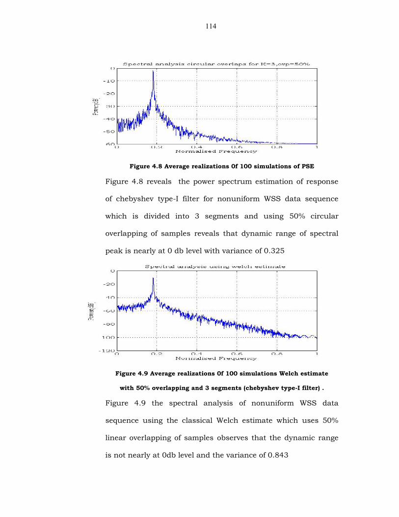
Figure 4.8 Average realizations 0f 100 simulations of PSE
Figure 4.8 reveals the power spectrum estimation of response
of chebyshev type-I filter for nonuniform WSS data sequence
which is divided into 3 segments and using 50% circular
overlapping of samples reveals that dynamic range of spectral
peak is nearly at 0 db level with variance of 0.325
Figure 4.9 Average realizations 0f 100 simulations Welch estimate
with 50% overlapping and 3 segments (chebyshev type-I filter) .
Figure 4.9 the spectral analysis of nonuniform WSS data
sequence using the classical Welch estimate which uses 50%
linear overlapping of samples observes that the dynamic range
is not nearly at 0db level and the variance of 0.843

115
Figure 4.10 True spectrum estimation of W.S.S Gaussian Ergodic
process.
Figure 4.10 shows that true power spectral density (PSD) of
nonuniform WSS data sequence with a dynamic range nearly at
0 dB and variance of 0.301
Figure 4.11 Comparison of spectral estimates for 50% overlapping
Figure 4.11 shows that the comparison of power spectrum estimate of
nonuniform WSS data sequences using circular overlapping of
samples provides less variance of 0.325 compare to Welch estimate
and true estimate, which provides variances of 0.843 and 0.301
respectively and also the range of circular estimate is at 0 dB level.

116
Figure 4.12 Average realizations 0f 100 simulations of PSE
Figure 4.12 shows that the power spectrum estimation of
response of chebyshev type-I filter for nonuniform WSS data
sequence which is divided into 3 segments and using 80%
circular overlapping of samples reveals that dynamic range of
spectral peak is nearly at10 dB level with variance of 0.318
Figure 4.13 Average realizations 0f 100 simulations Welch estimate
with 80% overlapping and 3 segments (chebyshev type-I filter) .
Figure 4.9 shows the spectral analysis of nonuniform WSS data
sequence using the classical Welch estimate which uses 80%
linear overlapping of samples observes that the dynamic range
is not nearly at 0db level and with the variance of 0.859

117
Figure 4.14 The true spectrum estimation of W.S.S Gaussian Ergodic
process.
Figure 4.14 it is observed that true power spectral density (PSD)
of nonuniform WSS data sequence having a dynamic range
nearly at 0 dB and a variance of 0.301
Figure 4.15 Comparison of spectral estimates for 80% overlapping
Figure 4.15 gives the comparison of power spectrum estimate of
nonuniform WSS data sequences using 80% circular overlapping of
samples provides variance of 0.318 compare to Welch estimate and
true estimate, which provides variances of 0.859 and 0.301
respectively.

118
Figure 4.16 Average realizations 0f 100 simulations of PSE
Figure 4.16 shows that the power spectrum estimation of response of
chebyshev type-I filter for nonuniform WSS data sequence which is
divided into 3 segments and using 100% circular overlapping of
samples reveals that dynamic range of spectral peak is nearly at 0 dB
level with variance of 0.305
Figure 4.17 Average realizations 0f 100 simulations Welch estimate
with 100% overlapping and 3 segments (chebyshev type-I filter) .
Figure 4.17 shows the spectral analysis of nonuniform WSS data
sequence using the classical Welch estimate which uses 100% linear
overlapping of samples observes that the dynamic range is not nearly
at 0db level and with the variance of 0.842
119
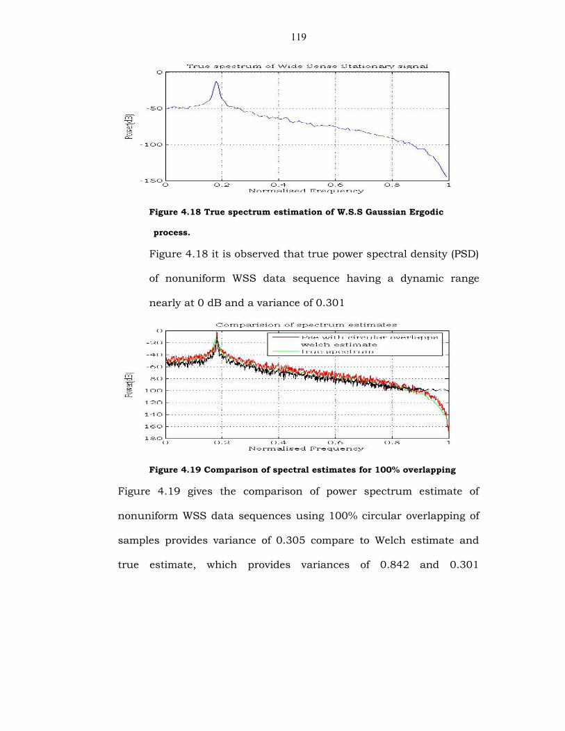
Figure 4.18 True spectrum estimation of W.S.S Gaussian Ergodic
process.
Figure 4.18 it is observed that true power spectral density (PSD)
of nonuniform WSS data sequence having a dynamic range
nearly at 0 dB and a variance of 0.301
Figure 4.19 Comparison of spectral estimates for 100% overlapping
Figure 4.19 gives the comparison of power spectrum estimate of
nonuniform WSS data sequences using 100% circular overlapping of
samples provides variance of 0.305 compare to Welch estimate and
true estimate, which provides variances of 0.842 and 0.301

120
respectively.
Figure 4.20 Average realizations of 100 simulations of PSE
Figure 4.20 gives the comparison of power spectrum estimate of
nonuniform WSS data sequences of 4 equal segments and using 60%
circular overlapping of samples provides variance of 0.192 compare to
Welch estimate, which provides variances of 0.756 and 0.301
respectively.
Figure 4.21 Average realizations of 100 simulations of PSE
Figure 4.21 gives the comparison of power spectrum estimate of
nonuniform WSS data sequences of 4 equal segments and using
70.5% circular overlapping of samples provides variance of 0.186
compare to Welch estimate, which provides variances of 0.716 and
0.301 respectively.

121
Figure 4.22 Average realizations of 100 simulations of PSE
Figure 4.22 gives the comparison of power spectrum estimate of
nonuniform WSS data sequences of 4 equal segments and using
76.6% circular overlapping of samples provides variance of 0.179
compare to Welch estimate, which provides variances of 0.741 and
0.301 respectively.
Figure 4.23 Average realizations 0f 100 simulations of PSE with circular
overlap with non overlapping and 3 segments (Butterworth filter).
Figure 4.23 the power spectrum estimation of response of Butterworth
filter for nonuniform WSS data sequence which is divided into 3
segments and using no circular overlapping of samples reveals that
minimum uncertainty is observed.

122
Figure 4.24 Average realizations 0f 100 simulations Welch estimate
with 0% overlapping and 3 segments (Butterworth filter) .
Figure 4.24 the power spectrum estimation of response of Butterworth
filter for nonuniform WSS data sequence which is divided into 3
segments and using no linear overlapping of samples reveals that
maximum uncertainty is observed in the above figure 4.24.
Figure 4.25 the true spectrum estimation of W.S.S Gaussian Ergodic
process.
Figure 4.25 provides the power spectrum estimation of response of
Butterworth filter for nonuniform WSS data sequence with the desired
amount of uncertainty is observed.

123
Figure 4.26 Comparison of spectral estimates for 0% overlapping
of samples.
Figure 4.26 reveals that PSE with circular overlapping reduces the
maximum uncertainty up to 20% then the PSE (Welch estimate) with
linear overlapping of samples.
Figure 4.27 Average realizations 0f 100 simulations of PSE with circular
overlap with non overlapping and 3 segments (Butterworth filter).
Figure 4.27 the power spectrum estimation of response of Butterworth
filter for nonuniform WSS data sequence which is divided into 3
segments and using 50% circular overlapping of samples reveals that
minimum uncertainty is observed.

124
Figure 4.28 Average realizations 0f 100 simulations Welch estimate
with 50% overlapping and 3 segments (Butterworth filter) .
Figure 4.28 the power spectrum estimation of response of Butterworth
filter for nonuniform WSS data sequence which is divided into 3
segments and using 50% linear overlapping of samples reveals that
maximum uncertainty is observed in the above figure 4.28.
Figure 4.29 The true spectrum estimation of W.S.S Gaussian Ergodic
process.
Figure 4.29 provides the power spectrum estimation of response of
Butterworth filter for nonuniform WSS data sequence with the desired
amount of uncertainty is observed.

125
Figure 4.30 Comparison of spectral estimates with 50% overlapping
of samples.
Figure 4.30 reveals that PSE with circular overlapping reduces the
maximum uncertainty up to 20% then the PSE (Welch estimate) with
linear overlapping of samples.
Figure 4.31 Average realizations 0f 100 simulations of PSE with circular
overlap with 80% overlapping and 3 segments (Butterworth filter).
Figure 4.31 the power spectrum estimation of response of Butterworth
filter for nonuniform WSS data sequence which is divided into 3
segments and using 80% circular overlapping of samples reveals that
minimum uncertainty is observed.

126
Figure 4.32 Average realizations 0f 100 simulations Welch estimate
with 80% overlapping and 3 segments (Butterworth filter) .
Figure 4.32 the power spectrum estimation of response of Butterworth
filter for nonuniform WSS data sequence which is divided into 3
segments and using 50% linear overlapping of samples reveals that
maximum uncertainty is observed in the above figure 4.32.
Figure 4.33 The true spectrum estimation of W.S.S Gaussian Ergodic
process.
Figure 4.33 provides the power spectrum estimation of response of
Butterworth filter for nonuniform WSS data sequence with the desired
amount of uncertainty is observed.

127
Figure 4.34 Comparison of spectral estimates with 80% overlapping
of samples.
Figure 4.34 reveals that PSE with circular overlapping reduces the
maximum uncertainty up to 20% then the PSE (Welch estimate) with
linear overlapping of samples.
Figure 4.35 Average realizations 0f 100 simulations of PSE with circular
overlap with 100% overlapping and 3 segments (Butterworth filter).
Figure 4.35 the power spectrum estimation of response of Butterworth
filter for nonuniform WSS data sequence which is divided into 3
segments and using 100% circular overlapping of samples reveals that
minimum uncertainty is observed.

128
Figure 4.36 Average realizations 0f 100 simulations Welch estimate
with 100% overlapping and 3 segments (Butterworth filter) .
Figure 4.36 the power spectrum estimation of response of Butterworth
filter for nonuniform WSS data sequence which is divided into 3
segments and using 80% linear overlapping of samples reveals that
maximum uncertainty is observed in the above figure 4.36.
Figure 4.37 The true spectrum estimation of W.S.S Gaussian Ergodic
process.
Figure 4.37 provides the power spectrum estimation of response of
Butterworth filter for nonuniform WSS data sequence with the desired
amount of uncertainty is observed.

129
Figure 4.38 Comparison of spectral estimates with 100% overlapping
of samples.
Figure 4.38 reveals that PSE with circular overlapping reduces the
maximum uncertainty up to 20% then the PSE (Welch estimate) with
linear overlapping of samples also the dynamic range using circular
overlapping of the samples observed near the 0 db level.
The Table 4.1 provides the variances for the Power spectrum
estimator using the circular overlapping of the samples with different
segments and different overlapping percentages.
Table 4.1 variance values for different percentages of overlapping
Variance(PXX(ω))/PXX2(ω) r=0 r=0.6 r=0.8 r=1
K=6 0.16 0.11 0.09 0.08
K=5 0.2 0.14 0.12 0.11
K=4 0.25 0.19 0.17 0.15
K=3 0.33 0.23 0.21 0.19
K=2 0.5 0.42 0.35 0.31

130
Figure 4.38: The variance versus the % of overlapping of PSE withnonlinear overlap.
Figure 4.38 reveals that in circular overlapping method the samples
exist for an equal number of times the sub records of data sequence,
by averaging these overlapping of samples of each sub record the
variance of the data sequence is further reduced.
4.26 Results and Discussions:
As the percentage overlapping of the samples increases the
variance is reduced as the case of chebyshev filter from Figure 4.4 to
Figure 4.22 to a minimum quantity and also for the case of
Butterworth filter as shown from Figure 4.23 to Figure 4.38, the bias
also approaches to true value hence the power spectrum estimation
with nonlinear overlapping of samples is said to be a consistent
estimate. Since in the circular overlapping method the samples are
existing for an equal number of times the sub records of data
sequence, by averaging these overlapping of samples of each sub
record the variance of the data sequence is further reduced. The

131
computation time is also reduced by 20% by allowing the samples to
have circular overlapping. Hence the power spectrum estimation with
circular overlapping of the samples is proposed over the linear
overlapping of samples to reduce the variance to smaller nonzero
quantity. The variances for different percentage of overlapping of
samples are tabulated in the Table 4.1 and from Figure 4.38 it can be
shown that the variance is reduced to lowest value for the increases of
percentage overlapping of samples. Hence we can conclude that the
power spectrum estimation with nonlinear overlapping of the samples
is an asymptotically consistent estimate for the nonuniform data
samples.
4.3 Power Spectrum estimation of nonuniform data in wide
dynamic range:
4.3.1 Introduction: Power spectral density (PSD) estimation
techniques are widely used in many applications, such as sonar,
radar, geophysics and biomedicine. Similar to single channel power
spectral density (PSD) estimation, there are basically two broad
categories of MPSD estimators. One is the nonparametric approach,
among which the Fourier-based estimators are the most popular. The
other is the parametric method, which assumes a model for the data.
Spectral estimation then becomes a problem of estimating the
parameters in the assumed model. The most commonly used model is
the autoregressive (AR) model because accurate estimates of the AR
parameters can be found by solving a set of linear equations .Similar
to the single channel case for short data records the Fourier-

132
based methods can suffer from significant bias problems while
AR model-based methods can suffer from inaccuracies in the
model as well as from imprecise model order selection.
Furthermore, some effective AR model-based approaches cannot be
easily extended to the multichannel case. In addition, as pointed out
by Jenkins and Watts, spurious cross-correlation or spurious
cross-spectral content may arise unless a prewhitening filter is
applied before PSD estimation. One such prewhitening filter was
suggested by Thomson for single channel PSD estimation.
The filter system function is given by kp1k z)k(a1)z(A and the
filter parameters a [1], a [2], a [3]…a[p]can be estimated from the data
using any AR-model based method. Denoting the output of this FIR
filter by u[n], a Fourier-based estimator is then used to generate the
PSD estimate )( fPu
. Finally, the PSD estimate of the original data is
found as
2
p1k
ux
fk2jexpka1
)f(P)f(P
(4.8)
where pa,...,2a,1a
are the estimated AR filter parameters. We term
this as the AR Prewhitened (ARPW) spectral estimator. Because of the
inconsistency of the definitions in the literature concerning MPSD
estimation, the following definitions will be made. A complex
multichannel sequence x[n] is defined as the complex 1L vector
x TL21 nX,...,nX,nXn where nX i represents the data

133
observed at the output of the ith channel and L is the number of
channels. For a wide sense stationary (WSS) multichannel random
process, the autocorrelation function (ACF) at lag k is defined as the
LL matrix function
nXKnXEkR HX
`
[k]LLr.[k]2Lr[k]1Lr::::[k]L2r.[k]22r[k]21r
[k]L1r...[k]12r[k]11r
(4.9)
where E[·] is the mathematical expectation, the superscript H denotes
conjugate transpose and krij is the cross-correlation function (CCF)
between nX i and nXj at lag k
nXknXEkr jiij (4.10)
For multichannel data of N samples, the sample vector, which is
1NL , is defined as
TTTTT 1NX,...,1X,...,1X,0XX (4.11)
The NLNL multichannel autocorrelation matrix of order N is
defined as
HXXERX (4.12)
.
0 0 1 ... 11 0 ... 2
.1 2 ... 0
Rx Rx Rx NRx Rx Rx N
Rx N Rx N Rx
it is seen that ,kRkR xxH so XR is hermitian. Because the
multichannel process is assumed to be wide sense stationary, XR is

134
also block Toeplitz. The power spectral density matrix or cross-
spectral matrix is defined as
)f(P...)f(P)f(P...
)f(P...)f(P)f(P)f(P...)f(P)f(P
)f(P
LL2L1L
...L22221
L11211
X
The diagonal elements Pii(f) are the PSDs of the individual channels or
auto-PSDs, while the off-diagonal elements Pil(f) for 1i are the
cross-PSDs between nX i and nX1 , which are defined as
fk2jexpkr)f(Pil il
(4.13)
The magnitude squared coherence (MSC) between channels i and j is
a quantity that indicates whether the spectral amplitude of the
process at a particular frequency in channel i is associated with large
or small spectral amplitude at the same frequency in channel j. It is
defined)t(jjP)f(iiP
)f(ijP)f(ij
22 (4.14)
A classic Fourier-based spectral estimator is the periodogram, which
is given as the LL matrix
)f(X)f(XN1)f(P H
PER (4.15)
where the Fourier transform is the L × 1 vector
).fn2jexp(nx)f(X1N
0n
(4.16)
The p th order AR model is defined as
135
nuinXiAnXp
1i
where pA,...,2A,1A are LL
AR coefficient matrices and nu is the excitation white noise or
kkRu and is the LL excitation noise covariance matrix
with being the discrete delta function.
The ARPW estimator given in (1) is readily extended to the
multichannel case. With the notations defined above, the
multichannel version of (1) is
)f(A)f(P)f(A)f(PH
u1
X
(4.17)
In addition to reducing spurious cross-spectral content, this
Prewhitened spectral estimator also gives an auto PSD spectral
estimate with much less bias than a Fourier based spectral estimator.
This is because the prewhitener reduces the dynamic range of the
PSD. However, this estimator is still inferior to the method proposed in
this paper. Instead of the FIR prewhitening filter, the proposed
estimator uses a prewhitening matrix, which is essentially a time
varying filter that is less susceptible to end effects. The new estimator
for a single channel PSD has been proposed in [4], while in this paper
it is extended to MPSD estimation. Assume the signal
1N,...,1,0n,nwnf2jAceXpnX O (4.18)
where nX is an 1L vector, Ac is an 1L complex amplitude to be
estimated, f0 is a known frequency, and
TTTT 1Nw,...,1w,0ww is a 1NL complex Gaussian noise

136
Whitenoise
e (n)x1(n)
vector with zero mean and known NLNL covariance matrix Rw .
The ML estimate of Ac is XREERoEA 1w
Ho
1
o1
wH
C
where X is the data sample vector and
LNL1Nf2jexpI,...,f2jexpI,IE T0L0LL0 with IL being an
LL identity matrix. The LL covariance matrix of this estimator is
1O
1w
HOCA EREC
(4.19)
Therefore, for a general WSS multichannel random process nX the
MVSE is defined as 1X1H )f(ER)f(Ep)f(PMV
where XR
is the estimated pLpL ACM of X and
.LpL1pf2jexpI,...,f2jexpI,I)f(E TLLL
4.3.2 Proposed System and Algorithm:
The proposed system and algorithm for the power spectrum estimator
is as shown below
)( fPx
Figure 4.39 Proposed system for ARPW spectral estimator
The nonuniform data sequence is generated using the Poisson
distributed sampling instants and also random distributed
sampling instants.
(15)
Estimated model
order ^p (EEF)criteria
Prewhitenmatrix Filter
NonParametricPSD
2)(1zH
AR(P)
)(1
)(zA
zH

137
The data sequence is generated using the given AR(P) process as
the white Gaussian noise with zero mean and unit variance as
the input for the system.
Choose a model order which fits for the AR(P) process using the
exponential embedded family criterion (EEF) for the given length
of the sequence.
Estimate the AR(P) coefficients using the Yule-Walker method
and so the AR model parameters for all the lower order models
are available.
Get residues at the output of a prediction error filter, the power
spectrum of the residues is evaluated using a nonparametric
technique as
The prewhitening technique increases the spectral flatness and
decreases the dynamic range of the residues.
To obtain the power spectrum estimation of data sequence in
wide dynamic range postcoloring technique is applied on the
spectrum of the residues
Segment the data into K equal length blocks, with LK .
Construct the LNLN matrix and 1XR using the estimated
parameters then average all the blocks to get the final estimate.
4.3.3 Simulation Results and Analysis:
To evaluate the effectiveness of the above algorithm, consider an
AR (4) process which has a wide dynamic range and a nonparametric
Welch estimate that suffers from leakage problem. The simulation
results are as shown in the following figures. Using the system
P
1k
*k )kn(xa)n(x)n(e 1NnP
)(eP)z(H)(P 2
X

138
function of the model
4321 z8978.0z7865.2z1012.4z6707.21
1)z(H
and white
Gaussian noise of zero mean and unit variance , input sequence is
generated for different lengths of 64,128,256and 512.The signal
samples are interpolated and then Prewhitened using the system
model to increase the spectral flatness to avoid leakage problem.
Figure 4.40 True estimate of AR(4) process for N=64.
Figure 4.40 provides the true power spectral density for the AR(4) data
sequence of length N=64 (nonuniform data sequence), the two spectral
peaks are clearly resolved and has the wide dynamic range power
levels.

139
Figure 4.41 Welch estimate, the two peaks are not resolve for N=64.
Figure 4.41 provides the Welch power spectral density for the AR(4)
data sequence of length N=64 (nonuniform data sequence), the two
spectral peaks are not clearly resolved and suffers from the spectral
leakage effects also it has no wide dynamic range of power levels.
Figure 4.42 Prewhitening estimate, two peaks are resolved for N=64.
Figure 4.42 provides the Prewhiten/postcolor estimate for the AR(4)
data sequence of length N=64 (nonuniform data sequence), the two
spectral peaks are clearly resolved and has wide dynamic range of
power levels.

140
Figure 4.43 Comparison of three estimates for N=64.
Figure 4.43 provides the Prewhiten/postcolor estimate for the AR(4)
data sequence of length N=64 (nonuniform data sequence), the two
spectral peaks are clearly resolved and has wide dynamic range of
power levels that is almost equivalent to the True spectrum whereas in
Welch estimate the two spectral peaks are not clearly resolved.
Figure 4.44 True estimate of AR(4) process for N=128.
Figure 4.44 provides the true power spectral density for the AR(4) data
sequence of length N=128 (nonuniform data sequence), the two
spectral peaks are clearly resolved and has the large dynamic range
power levels.

141
Figure 4.45 Welch estimate, the two peaks are not resolved for N=128.
Figure 4.45 provides the Welch power spectral density for the AR(4)
data sequence of length N=128 (nonuniform data sequence), the two
spectral peaks are not clearly resolved and suffers from the spectral
leakage effects also it has no wide dynamic range of power levels.
Figure 4.46 Prewhitening estimate, two peaks are resolved for N=128.
Figure 4.46 provides the Prewhiten/postcolor estimate for the AR(4)
data sequence of length N=128 (nonuniform data sequence), the two
spectral peaks are clearly resolved and has wide dynamic range of
power levels.

142
Figure 4.47 Comparison of three estimates for N=128.
Figure 4.47 provides the Prewhiten/postcolor estimate for the AR(4)
data sequence of length N=128 (nonuniform data sequence), the two
spectral peaks are clearly resolved and has wide dynamic range of
power levels that is almost equivalent to the True spectrum whereas in
Welch estimate the two spectral peaks are not clearly resolved.
Figure 4.48 True estimate of AR(4) process for N=256.
Figure 4.48 provides the true power spectral density for the AR(4) data
sequence of length N=256 (nonuniform data sequence), the two
spectral peaks are clearly resolved and has the large dynamic range
power levels.

143
Figure 4.49 Welch estimate, the two peaks are not resolve for N=256.
Figure 4.49 provides the Welch power spectral density for the AR(4)
data sequence of length N=256 (nonuniform data sequence), the two
spectral peaks are just begin to resolve and suffers from the spectral
leakage effects also it has narrow dynamic range of power levels.
Figure 4.50 Prewhitening estimate, two peaks are resolved for N=256.
Figure 4.50 provides the Prewhiten/postcolor estimate for the AR(4)
data sequence of length N=256 (nonuniform data sequence), the two
spectral peaks are clearly resolved and has wide dynamic range of
power levels.

144
Figure 4.51 Comparison of three estimates for N=256.
Figure 4.51 provides the Prewhiten/postcolor estimate for the AR(4)
data sequence of length N=256 (nonuniform data sequence), the two
spectral peaks are clearly resolved and has wide dynamic range of
power levels that is almost equivalent to the True spectrum whereas in
Welch estimate the two spectral peaks are not clearly resolved.
Figure 4.52 True estimate of AR(4) process for N=512.
Figure 4.52 provides the true power spectral density for the AR(4) data
sequence of length N=512 (nonuniform data sequence), the two
spectral peaks are clearly resolved and has the large dynamic range of
power levels.

145
Figure 4.53 Welch estimate, the two peaks are not resolve for N=512.
Figure 4.53 provides the Welch power spectral density for the AR(4)
data sequence of length N=512 (nonuniform data sequence), the two
spectral peaks are resolved but suffers from the spectral leakage
effects also it has narrow dynamic range of power levels.
Figure 4.54 Prewhitening estimate, two peaks are resolved for N=64.
Figure 4.54 provides the Prewhiten/postcolor estimate for the AR(4)
data sequence of length N=512 (nonuniform data sequence), the two
spectral peaks are clearly resolved and has wide dynamic range of
power levels.

146
Figure 4.55 Comparison of three estimates for N=512.
Figure 4.55 provides the Prewhiten/postcolor estimate for the AR(4)
data sequence of length N=512 (nonuniform data sequence), the two
spectral peaks are clearly resolved and has wide dynamic range of
power levels that is equivalent to the true spectrum whereas in Welch
estimate the two spectral peaks are resolved with small range of power
levels.
4.34 Conclusions: As we know, the nonparametric methods do not
resolve the two peaks in true spectrum and suffers from leakage at
high frequencies. Hence the combination of nonparametric with
parametric resolves two peaks with ease also follows the true
spectrum. By observing from Figure 4.40 to Figure 4.55, the two
peaks are not resolved in the Welch estimate for lesser amount of data
samples(N=64) whereas in the proposed estimate the two peaks are
resolved. If we increase the number of samples from N=64 to N=256,
the existing Welch estimate does not resolve the two spectral peaks,
on the other hand using the prewhitening and post coloring method
the two spectral peaks are greatly resolved. Therefore the use of

147
parametric method as a preprocessor is highly recommended in the
wide dynamic range of spectral estimations.
4.4 Power spectrum estimation using interpolation techniques:
4.4.1 Introduction: The power spectral analysis of uniformly sampled
data is a well known topic. We are having enough number of regularly
sampled methods for appropriate applications. The survey suggests
that the analysis of nonuniformly sampled data sequences is also to
be considered. The purpose for the analysis of nonuniform data
sequence includes in the applications such as oceanic data,
biomedicine, seismology, astronomy, and particularly in economics
data is nonuniform rather than uniformly sampled data. Hence the
power spectral analysis of nonuniform data sequence is some what
under developed data.
The power spectrum estimation of uneven and nonuniformly
sampled random sequences can be carried out by least squares
periodogram (LSP), and coherent sampling methods. The proposed
algorithm for the estimation of nonuniform random sequences uses
the interpolation methods as resampling methods thus eliminates the
low pass filtering effects and also Lomb transforms as well as weighted
least squares methods are suggested.
The computational methods used in digital computer for the
evaluation of the library functions, such as sin(x), cos (x), requires
polynomial approximations using Taylor series. The data required to
construct a Taylor polynomial is the value of the function f(x) and its

148
derivative. The main disadvantage of this method is to know the
higher order derivatives which are hard to compute.
In statistical signal analysis and scientific analysis arise the
situations where the function y=f(x) is available only for N+1 tabulated
data values, and a technique is needed to approximate the function
f(x) at nontabulated abscissas. If there are a significant amount of
errors in the tabulated values the curve fitting techniques are used.
On the other hand if the points are known to have a high degree of
accuracy, then a polynomial curve p(x) that passes through them is
considered. When the polynomial approximation is considered within
an interval, the approximation p(x) is called an interpolated value. If
the approximation is considered outside the interval, then p(x) is
called an extrapolated value. Polynomials are used to design
algorithms to approximate functions, for numerical differentiation, for
numerical integration and for making computer drawn curves that
must pass through specified points.
Polynomial interpolation for a set N+1 points Nkkkx yx 0, is
generally not quite approximated. A polynomial of degree N can have
N-1 number of maxima and minima, and the graph can wiggle in
order to pass through the points. Another method is to piece together
the graphs of lower degree polynomials )(xS k and interpolate between
the successive nodes ),(,, 11 kkkx yxyx . The set of the function forms a
piecewise polynomial curve. Interpolation is a technique of making a
perfect approximation of given function within the interval of values.

149
Different interpolation techniques involve linear interpolation and
cubic spline interpolation. The linear interpolation involves the linear
relationship of the interval values whereas the cubic interpolation
involves the nonlinear relationship of the interval values. A different
cubic spline technique involves clamped spline, natural spline,
extrapolated spline, parabolically terminated spline and endpoint
curvature adjusted spline. A practical feature of splines is the
minimum of oscillatory behavior that they posses.
Unevenly or nonuniformly sampled data sequences are not
sampled with the Nyquist rates. Hence these data sequences require
resampling methods. Linear interpolation and cubicspline
interpolation techniques are employed as resampling methods to
estimate the power of the nonuniform data sequences.
The least squares spectral analysis is a technique of estimating
the power spectrum of nonuniformly sampled sequences based on the
least squares fit of sinusoids to data sequences. In this method data
sequences are approximated using the weighted sum of sinusoidal
frequency components using a linear regression method or a least
squares fit method. The number of sinusoids that are used for
approximation should be less than or equal to the number of data
samples. A data vector Y can be represented as a weighted sum of
sinusoids as AXY . The elements of the matrix A can be calculated
by evaluating each function at the sampling time instants, with the
weighted vector X . The weighted vector x is chosen such that to
minimize the sum of squared errors in approximating the data vector

150
Y and the solution for X is given as a closed form AYAAX1T
where the matrix AAT is a diagonal matrix. Then the power spectrum
estimate using the interpolated least squares spectral analysis can be
given by
XAXA
N1)(P
T
IS .
4.4.2 Algorithm:
The block diagram and algorithm for power spectrum estimation
using proposed techniques is as follows.
Generate nonuniform data sequences of different lengths ‘N’.
Interpolate the data sequences Nk0kkx y,x within the interval
of values N0 x,x .
By applying the Linear as well as Cubic Spline interpolation
techniques within the interval N0 x,x , the data sequence is
approximated as x (n).
Figure4.56 (i) Proposed system model.
AR (P)Filter
PeriodogramAnalysis
Input datax (n)
WhiteNoise w (n)
PeriodogramUsing WLSP
PeriodogramUsing LSP
Y(n)
Non Parametric SpectrumMethods
Pxx(ω)
PWLSP(ω)
PLS ω)
+

151
The power spectrum of the interpolated data sequence x(n) is
calculated employing the nonparametric methods.
XAXA
N1)(P
T
IS
The Lomb periodogram is evaluated for the nonuniform data
sequence
N
1nn
2
2N
1nn
N
1nn
2
2N
1nn
xx))t((sin
))t(sin()tn(x
))t((cos
))t(cos()tn(x
21)(P
where is defined by)2cos(
)t2sin()2tan( N
1nn
N
1nn
The weighted least squares periodogram can be given by
XAXAba
N1)(P
T22
WLSP , where ‘a’ and ‘b’ are data
dependent weights and ‘A’ is the data dependent matrix.
4.4.3 Simulation Analysis:
The simulations results for the nonuniform data sequences of
white Gaussian noise, real sinusoids in Gaussian noise and narrow
band sinusoidal components in broad band noise are illustrated as
follows. The Interpolation methods are employed as resampling
methods to convert the nonuniformly sampled sequences into
uniformly sampled sequences. The proposed interpolation techniques
employed are linear and cubic spline interpolation techniques. The
simulation results are observed for both the interpolation techniques

152
and are compared to the least squares methods and Lomb transform
methods.
Figure 4.56 Real sinusoids in white Gaussian noise for N=30.
Figure 4.56 provides the real sinusoidal components in nonuniform
data sequence of white Gaussian noise of length 30. The figure shows
the amplitude versus time index of Gaussian noise.
Figure 4.57 Interpolated random sequence using linear interpolation.
Figure 4.57 provides the linear interpolated data sequence of white
Gaussian noise of length N=30 using linear interpolation technique
which converts the nonuniform data sequence to uniformly sampled
sequence with sampling period of 1 sec.

153
Figure 4.58 Periodogram analysis for the random sequence of N=30.
Figure 4.58 provides the nonparametric power spectrum estimation
using the periodogram technique having the spectral component at
0.5 normalized frequency with power levels of 680 dBs and no other
components are exists below 0.2 normalized frequencies.
Figure 4.59 Spectral analysis of random sequence using linear interpolation
Figure 4.59 provides spectrum analysis using proposed linear
interpolation technique shows that there spectral components existing
even below 0.2 normalized frequency and are at 0.08, 0.1, and 0.15
frequencies respectively with good power levels above 800dbs which
were not visible in the classical nonparametric periodogram
estimation.
154
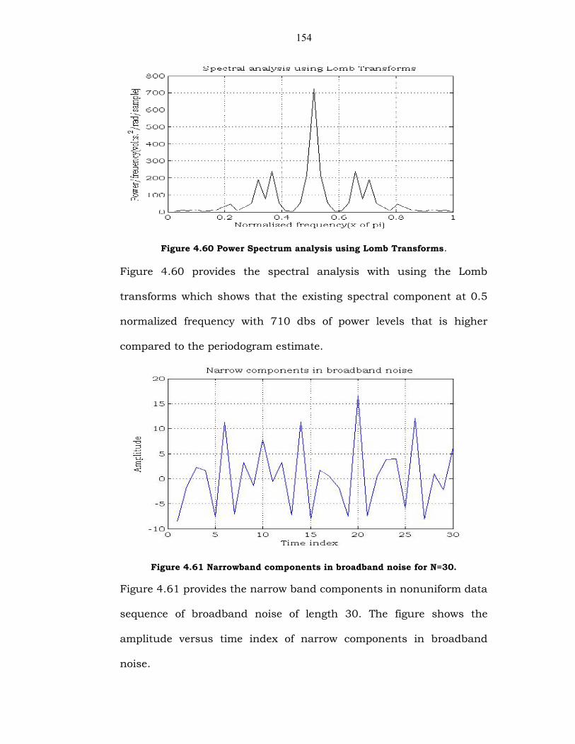
Figure 4.60 Power Spectrum analysis using Lomb Transforms.
Figure 4.60 provides the spectral analysis with using the Lomb
transforms which shows that the existing spectral component at 0.5
normalized frequency with 710 dbs of power levels that is higher
compared to the periodogram estimate.
Figure 4.61 Narrowband components in broadband noise for N=30.
Figure 4.61 provides the narrow band components in nonuniform data
sequence of broadband noise of length 30. The figure shows the
amplitude versus time index of narrow components in broadband
noise.
155
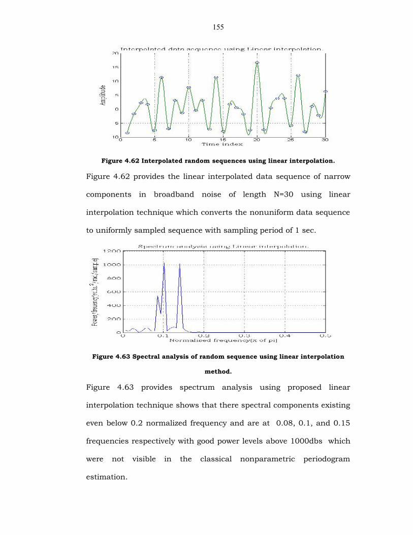
Figure 4.62 Interpolated random sequences using linear interpolation.
Figure 4.62 provides the linear interpolated data sequence of narrow
components in broadband noise of length N=30 using linear
interpolation technique which converts the nonuniform data sequence
to uniformly sampled sequence with sampling period of 1 sec.
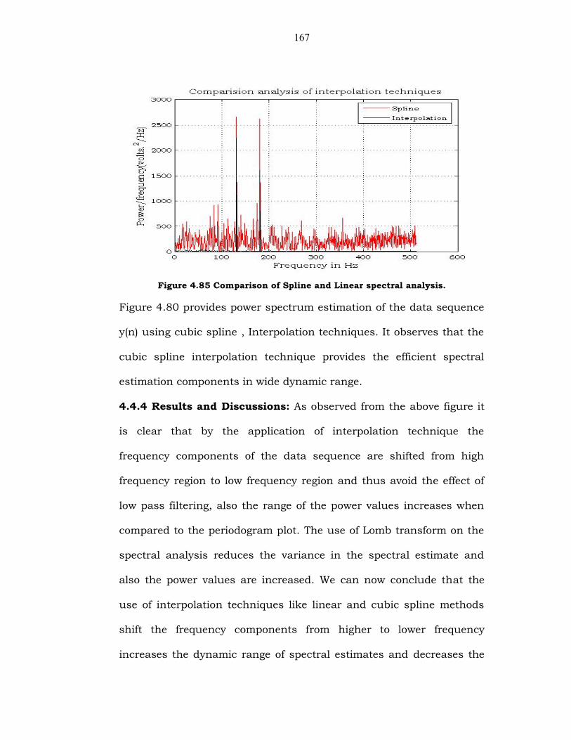
Figure 4.63 Spectral analysis of random sequence using linear interpolation
method.
Figure 4.63 provides spectrum analysis using proposed linear
interpolation technique shows that there spectral components existing
even below 0.2 normalized frequency and are at 0.08, 0.1, and 0.15
frequencies respectively with good power levels above 1000dbs which
were not visible in the classical nonparametric periodogram
estimation.

156
Figure 4.64 Power Spectrum analysis using Lomb Transforms.
Figure 4.64 provides the spectral analysis with using the Lomb
transforms of narrow band components in broadband noise of length
30 which shows that the existing spectral component at 0.5
normalized frequency with 710 dbs of power levels that is higher
compared to the periodogram estimate.
Figure 4.65 Nonuniformly sampled white Gaussian Noise AWN(0,1) for N=30.
Figure 4.65 provides the nonuniformly sampled white Gaussian noise
of length N=30 .The figure shows the amplitude versus time index of
white Gaussian noise.

157
Figure 4.66 Spectrum analysis using the periodogram.
Figure 4.66 provides the nonparametric power spectrum estimation
using the periodogram technique having the spectral component at
0.5 rad/sample normalized frequency with power levels of 0.09 dBs
and the other components are exists with power levels of 0.052 dBs
and 0.06 dBs.
Figure 4.67 Spectral analysis using Least Squares Periodogram.
Figure 4.67 provides power spectrum estimation using the Least
squares periodogram technique having the spectral component at 0.5
normalized frequency with power levels of 0.18 dBs and the other
components are exists with power levels above 0.1 dBs.

158
Figure 4.68 Comparison of spectral estimates for LSP and Periodogram.
Figure 4.68 provides the comparison of two spectral estimates using
Least squares periodogram and periodogram techniques. In LSP
technique the power levels are increased than the power levels of
periodogram by more than 100% so that one can realize the noise
spectral components in the signal content.
Figure 4.69 Nonuniformly sampled real sinusoids in AWN(0,1) for N=30.
Figure 4.69 provides the nonuniformly sampled real sinusoids in
white Gaussian noise of length N=30 .The figure shows the amplitude
versus time index of white Gaussian noise.

159
Figure 4.70 Spectrum analysis using the periodogram.
Figure 4.70 provides the nonparametric power spectrum estimation
using the periodogram technique having the spectral component at
0.5 rad/sample normalized frequency with power levels of 6.5 dBs and
the other components exists with power levels of 3 dBs and 1 dBs.
Figure 4.71 Spectral analysis using Least Squares Periodogram.
Figure 4.71 provides power spectrum estimation using the Least
squares periodogram technique having the spectral component at 0.5
normalized frequency with power levels of 13 dBs and the other
components are exists with power levels above 2.2dBs and 6 dBs.

160
Figure 4.72 Comparison of spectral estimates for LSP and Periodogram.
Figure 4.72 provides the comparison of two spectral estimates using
Least squares periodogram and periodogram techniques. In LSP
technique the power levels are increased than the power levels of
periodogram by more than 100% so that one can realize the noise
spectral components in the signal content.

161
Figure 4.73 Nonuniformly sampled narrowband components in wideband noise
Figure 4.73 provides the nonuniformly sampled narrowband
components in wideband noise of length N=30 .The figure shows the
amplitude versus time index of white Gaussian noise.
Figure 4.74 Spectral analysis using Periodogram for N=30.
Figure 4.74 provides the nonparametric power spectrum estimation
using the periodogram technique having the spectral component at
0.5 rad/sample normalized frequency with power levels of 6.5 dBs and
the other components exists with power levels of 3 dBs and 2 dBs
respectively.

162
Figure 4.75 Spectral analysis using Least Squares Periodogram.
Figure 4.75 provides power spectrum estimation using the Least
squares periodogram technique having the spectral component at 0.5
normalized frequency with power levels of 13 dBs and the other
components are exists with power levels of 6dBs and 4 dBs.
Figure 4.76 Comparison of spectral estimates for LSP and Periodogram.
Figure 4.76 provides the comparison of two spectral estimates using
Least squares periodogram and periodogram techniques. In LSP
technique the power levels are increased than the power levels of
periodogram by more than 150% so that one can realize the noise
spectral components in the signal content.

163
Figure 4.77 periodogram analysis for the data sequence of length N=256
)1.0cos(4)952.0cos(4)04.0cos(2)( 321 nnnny
Figure 4.77 provides power spectrum estimation of the above data
sequence y(n) using the periodogram technique having the spectral
component at 0.04 , 0.952 and 0.1 normalized frequencies. It observes
that two spectral peaks at 0.952 and 0.1 normalized frequencies are
not properly resolved.
Figure 4.78Least squares periodogram analysis for the data sequence of length
N=256 )1.0cos(4)952.0cos(4)04.0cos(2)( 321 nnnny
Figure 4.78 provides power spectrum estimation of the above data
sequence y (n) using the Least squares periodogram technique having
the spectral component at 0.04, 0.952 and 0.1 normalized
frequencies. It observes that two spectral peaks at 0.952 and 0.1
normalized frequencies are clearly resolved.

164
Figure 4.79 Weighted Least Squares Periodogram analysis for the data
sequence )1.0cos(4)952.0cos(4)04.0cos(2)( 321 nnnny
Figure 4.79 provides power spectrum estimation of the above data
sequence y(n) using the weighted Least squares periodogram
technique having the spectral component at 0.04 , 0.952 and 0.1
normalized frequencies. It observes that two spectral peaks at 0.952
and 0.1 normalized frequencies are clearly resolved with wide dynamic
range of 20 to 40 dBs.
Figure 4.80 Comparison of Periodogram, LSP and WLSP.
Figure 4.80 provides power spectrum estimation of the above data
sequence y(n) using the periodogram , LSP and WLSP techniques. It
observes that the Weighted Least Squares periodogram technique
provides the efficient spectral estimation components in wide dynamic
range with less variance compared to other methods.

165
Figure 4.81 Nonuniform data sequence.
Figure 4.81 provides the discrete non uniform data sequence with
amplitude versus time index plot. It observes that all the samples are
randomly spaced within the time interval 0 to 1 second.
Figure 4.82 Linear interpolations of nonuniform data
Figure 4.82 provides the linear interpolation of discrete non uniform
data sequence with amplitude versus time index plot. It observes that
all the samples are uniformly spaced after applying the interpolation
technique within the time interval 0 to 1 second.

166
Figure 4.83 Cubic spline interpolation of nonuniform data.
Figure 4.83 provides the cubic spline interpolation of discrete non
uniform data sequence with amplitude versus time index plot. It
observes that all the samples are uniformly spaced after applying the
interpolation technique within the time interval 0 to 1 second.
Figure 4.84 Spectral analysis using cubic spline interpolation.
Figure 4.84 provides the cubic spline interpolation of discrete non
uniform data sequence with amplitude versus time index plot. It
observes that all the samples are uniformly spaced after applying the
interpolation technique within the time interval 0 to 1 second.
167
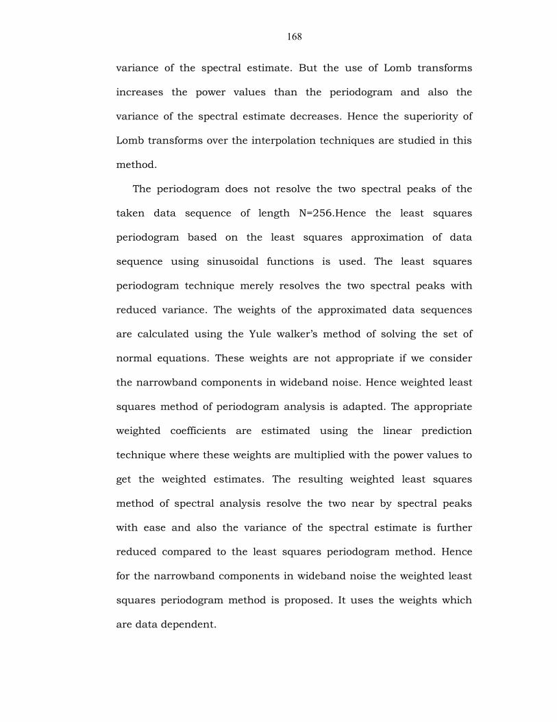
Figure 4.85 Comparison of Spline and Linear spectral analysis.
Figure 4.80 provides power spectrum estimation of the data sequence
y(n) using cubic spline , Interpolation techniques. It observes that the
cubic spline interpolation technique provides the efficient spectral
estimation components in wide dynamic range.
4.4.4 Results and Discussions: As observed from the above figure it
is clear that by the application of interpolation technique the
frequency components of the data sequence are shifted from high
frequency region to low frequency region and thus avoid the effect of
low pass filtering, also the range of the power values increases when
compared to the periodogram plot. The use of Lomb transform on the
spectral analysis reduces the variance in the spectral estimate and
also the power values are increased. We can now conclude that the
use of interpolation techniques like linear and cubic spline methods
shift the frequency components from higher to lower frequency
increases the dynamic range of spectral estimates and decreases the
168
variance of the spectral estimate. But the use of Lomb transforms
increases the power values than the periodogram and also the
variance of the spectral estimate decreases. Hence the superiority of
Lomb transforms over the interpolation techniques are studied in this
method.
The periodogram does not resolve the two spectral peaks of the
taken data sequence of length N=256.Hence the least squares
periodogram based on the least squares approximation of data
sequence using sinusoidal functions is used. The least squares
periodogram technique merely resolves the two spectral peaks with
reduced variance. The weights of the approximated data sequences
are calculated using the Yule walker’s method of solving the set of
normal equations. These weights are not appropriate if we consider
the narrowband components in wideband noise. Hence weighted least
squares method of periodogram analysis is adapted. The appropriate
weighted coefficients are estimated using the linear prediction
technique where these weights are multiplied with the power values to
get the weighted estimates. The resulting weighted least squares
method of spectral analysis resolve the two near by spectral peaks
with ease and also the variance of the spectral estimate is further
reduced compared to the least squares periodogram method. Hence
for the narrowband components in wideband noise the weighted least
squares periodogram method is proposed. It uses the weights which
are data dependent.


![Afirst-orderprimal-dualalgorithmwithlinesearch · 2016. 8. 31. · Our proposed analysis of PDA exploits the idea of recent works [13,14] where are proposed several algorithms for](https://img.dokumen.tips/doc/110x75/5fe94138e4714b5ae6389125/airst-orderprimal-dualalgori-2016-8-31-our-proposed-analysis-of-pda-exploits.jpg)


![Performance Comparison of Evolutionary Algorithms for ... · [22] proposed the use of cultural algorithms which incorporate knowledge to the algorithm to solve UCTP instances; they](https://img.dokumen.tips/doc/110x75/5e75f92637b178152c276232/performance-comparison-of-evolutionary-algorithms-for-22-proposed-the-use.jpg)