SPATIAL DISTRIBUTION OF WATER SUPPLY IN THE … · SPATIAL DISTRIBUTION OF WATER SUPPLY IN THE COTERMINOUS UNITED STATES1 ... Spatial Distribution of Water Supply in ... and dries

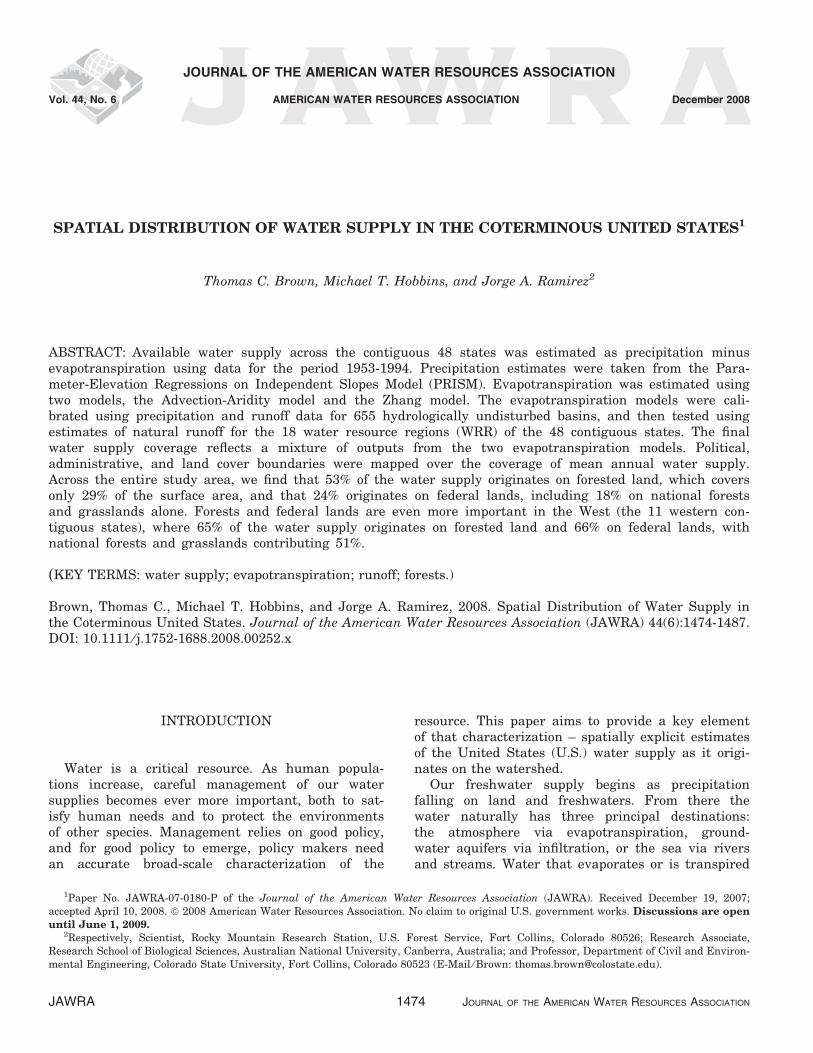
SPATIAL DISTRIBUTION OF WATER SUPPLY IN THE COTERMINOUS UNITED STATES1

Thomas C. Brown, Michael T. Hobbins, and Jorge A. Ramirez2

ABSTRACT: Available water supply across the contiguous 48 states was estimated as precipitation minusevapotranspiration using data for the period 1953-1994. Precipitation estimates were taken from the Para-meter-Elevation Regressions on Independent Slopes Model (PRISM). Evapotranspiration was estimated usingtwo models, the Advection-Aridity model and the Zhang model. The evapotranspiration models were cali-brated using precipitation and runoff data for 655 hydrologically undisturbed basins, and then tested usingestimates of natural runoff for the 18 water resource regions (WRR) of the 48 contiguous states. The finalwater supply coverage reflects a mixture of outputs from the two evapotranspiration models. Political,administrative, and land cover boundaries were mapped over the coverage of mean annual water supply.Across the entire study area, we find that 53% of the water supply originates on forested land, which coversonly 29% of the surface area, and that 24% originates on federal lands, including 18% on national forestsand grasslands alone. Forests and federal lands are even more important in the West (the 11 western con-tiguous states), where 65% of the water supply originates on forested land and 66% on federal lands, withnational forests and grasslands contributing 51%.

(KEY TERMS: water supply; evapotranspiration; runoff; forests.)

Brown, Thomas C., Michael T. Hobbins, and Jorge A. Ramirez, 2008. Spatial Distribution of Water Supply inthe Coterminous United States. Journal of the American Water Resources Association (JAWRA) 44(6):1474-1487.DOI: 10.1111 ⁄ j.1752-1688.2008.00252.x

INTRODUCTION

Water is a critical resource. As human popula-tions increase, careful management of our watersupplies becomes ever more important, both to sat-isfy human needs and to protect the environmentsof other species. Management relies on good policy,and for good policy to emerge, policy makers needan accurate broad-scale characterization of the

resource. This paper aims to provide a key elementof that characterization – spatially explicit estimatesof the United States (U.S.) water supply as it origi-nates on the watershed.

Our freshwater supply begins as precipitationfalling on land and freshwaters. From there thewater naturally has three principal destinations:the atmosphere via evapotranspiration, ground-water aquifers via infiltration, or the sea via riversand streams. Water that evaporates or is transpired

1Paper No. JAWRA-07-0180-P of the Journal of the American Water Resources Association (JAWRA). Received December 19, 2007;accepted April 10, 2008. ª 2008 American Water Resources Association. No claim to original U.S. government works. Discussions are openuntil June 1, 2009.

2Respectively, Scientist, Rocky Mountain Research Station, U.S. Forest Service, Fort Collins, Colorado 80526; Research Associate,Research School of Biological Sciences, Australian National University, Canberra, Australia; and Professor, Department of Civil and Environ-mental Engineering, Colorado State University, Fort Collins, Colorado 80523 (E-Mail ⁄ Brown: [email protected]).

JAWRA 1474 JOURNAL OF THE AMERICAN WATER RESOURCES ASSOCIATION

JOURNAL OF THE AMERICAN WATER RESOURCES ASSOCIATION

Vol. 44, No. 6 AMERICAN WATER RESOURCES ASSOCIATION December 2008

has largely escaped our grasp until it falls againelsewhere as precipitation. What remains is – untilit reaches the sea – available for use by humansand other species, and in a broad sense is ourfreshwater supply.

As much of our water supply originates in forests,water runoff and its quality have long been a focus offorest management. The first national forest preserveswere specifically set aside by Congress in the OrganicAct of 1897 for the protection of water and timbersupplies. Although national forests cover only 8% ofthe land area in the contiguous 48 states, they are ofparticular interest because they are generally locatedat basin headwaters. Various estimates of the propor-tion of the nation’s water supply originating onnational forests, and on forests in general, have beensuggested over the years. For example, a 1970 reviewof public lands estimated that in the 11 contiguouswestern states 61% of the natural runoff originated onfederal lands, with 54% coming from the nationalforests (Public Land Law Review Commission, 1970),and more recently a Forest Service report estimatedthat 14% of the water supply of the 48 states and 33%of the water supply of the West originated on nationalforests (Sedell et al., 2000). Using newer data and mod-els, we aimed to provide an improved set of estimates.

The approach taken here was to estimate watersupply at its source as precipitation minus evapo-transpiration for each cell of a grid covering the con-tiguous 48 states (Alaska and Hawaii were excludedbecause of lack of data). Overlaying political and landownership boundaries or land cover delineations thenallows estimation of the amount of water originatingwithin distinct land units.

We took our precipitation estimates from a well-established model. Estimating evapotranspiration wasmore challenging, and we examined two quite differ-ent models. Finding that neither model estimatedevapotranspiration with sufficient accuracy in alllocations, and focusing clearly on our very practicalobjective of estimating mean annual contribution towater supply, we calibrated each model to improvethe accuracy of the estimates, and then used one orthe other model in specific basins where furthertesting indicated that it yielded the more accurateestimate. Next we explain the methods in some detail.

METHODS

Our basic approach was to estimate water supply(Q) as precipitation (P) minus actual evapotranspira-tion (ETa) on a mean annual basis at each 5 · 5-kmgrid cell across the conterminous U.S.

Q ¼ P� ETa ð1Þ

Having these spatially distributed estimates ofwater supply at its source, boundaries were thenoverlaid. Aggregating estimates of Q across cellswithin a boundary indicates the amount of water sup-ply originating within the designated area.

The logic of estimating mean annual Q as P ) ETa

relies on assumptions involving basin storage. Morespecifically, Q is

Q ¼ P� ETa � DSs � DSg ð2Þ

where DS represents changes in storage and sub-scripts s and g refer to surface and subsurfacedomains. Assuming a stable climate and an undis-turbed basin, the long-term average annual netchange in overall basin moisture storage is negligi-ble and assumed to be 0, so Q devolves to Equation(1).

Precipitation is the most commonly measuredhydrologic quantity, but because precipitation is spa-tially variable, especially in mountainous regions,models are needed for filling in between the locationsof precipitation gages. For this purpose we selectedthe monthly precipitation estimates produced at a5-km level of resolution by the Parameter-ElevationRegressions on Independent Slopes Model (PRISM)(Daly et al., 1994). PRISM combines climatologic andtopographic data to interpolate between precipitationobservations.

For ETa we set out to adapt the Advection-Aridity(AA) model (Brutsaert and Stricker, 1979) for nation-wide use. A subsidiary aim was to develop a modelfor estimating ETa at the monthly time scale thatcould be applied over the contiguous U.S., whichcould then be used in other analyses that are not atissue here. The AA model is based on the complemen-tary relationship of actual and potential evapotrans-piration, described below, and relies largely onreadily available weather data.

Unfortunately, the AA model was not able accu-rately to estimate ETa for some areas of the U.S.,largely because of insufficient data. In locationswhere the AA model performed poorly we usedanother model, one proposed by Zhang et al. (2001).The Zhang model employs a very different theoreti-cal approach from that of the complementary rela-tionship and estimates ETa on a mean annual basisonly. The loss of seasonality with the Zhang modelwas not a shortcoming in the current context, asour objective here is to estimate mean annualwater supply. Both models are described brieflybelow, as are methods for model calibration andtesting.

SPATIAL DISTRIBUTION OF WATER SUPPLY IN THE COTERMINOUS UNITED STATES

JOURNAL OF THE AMERICAN WATER RESOURCES ASSOCIATION 1475 JAWRA

The AA Model for Estimating ETa

In hydrology it has been customary to model ETa

as a function of potential evapotranspiration (ETp)and soil moisture, where ETp is the evapotrans-piration that would theoretically occur were waternot limiting. In this approach, ETp is considered anindependent climatic variable, constraining theamount of ETa but remaining unaffected by theamount of ETa and thus largely constant over rangesof actual moisture availability at a given location.However, as proposed by Bouchet (1963), ETp is notunaffected by ETa. Rather, when lack of soil moisturekeeps ETa below the level that available energywould support (i.e., ETp), the surplus energy heatsand dries the surrounding air, raising ETp abovewhat it would be if more moisture were available andETa were greater. When moisture is not limiting, ETa

equals ETp at a rate referred to as wet environmentevapotranspiration (ETw). However, as Bouchetproposed, at regional scales and away from sharpenvironmental discontinuities, if moisture is limitingand the available energy is constant, energy not usedfor ETa causes ETp to rise above ETw by the amountthat ETa falls below it

ETa þ ETp ¼ 2ETw ð3Þ

Figure 1 illustrates the complementary relationship.Complementary relationship models rely largely on

atmospheric observations. The models avoid the needfor data on soil moisture, stomatal resistance proper-ties of the vegetation, or other surface aridity mea-sures because vertical gradients of temperature andhumidity in the atmospheric boundary layer reflectthe presence of moisture availability at the surface.

Models based on the complementary relationshiphypothesis have been successfully used to make pre-dictions of regional ETa at different temporal scales,

thereby providing indirect evidence of its validity(Brutsaert and Stricker, 1979; Morton, 1983; Hobbinset al., 2001a; Szilagyi, 2001). Furthermore, thecomplementary relationship has recently beendemonstrated observationally with data from a set ofsites across the freeze-free zone of the U.S. usingannual pan evaporation measures to estimate ETp,denoted here as ET�p, and a water balance approachto estimate ETa, denoted here as ET�a (Hobbins et al.,2004b). The water balance approach simply computesannual ET�a as precipitation (P) minus basin watersupply estimated as streamflow (Q*) from thewatersheds surrounding the pans

ET �a ¼ P�Q� ð4Þ

Plots of annual ET�p and ET�a matched closely thelines for ETp and ETa in Figure 1 (Hobbins et al.,2004b; Ramirez et al., 2005).

Several complementary relationship models are nowavailable, the most widely known of which are theComplementary Relationship Areal Evapotrans-piration (CRAE) model (Morton, 1983) and the AAmodel (Brutsaert and Stricker, 1979). Hobbins et al.(2001b) compared these two models for ability toestimate ETa across the U.S. and selected the AAmodel as the most promising approach for such anapplication. In this model, ETw is calculated based onderivations of the concept of equilibrium evapotranspi-ration under conditions of minimal advection, firstproposed by Priestley and Taylor (1972), and ETp iscalculated by combining information from the energybudget and water vapor transfer in the Penmanequation (Penman, 1948) [see Hobbins et al. (2001a)for details on the modified AA model that weemployed].

Data for the AA Model. The AA model of ETa

requires data on temperature, humidity, solarradiation, wind speed, albedo, elevation, and latitude.Most of the available climatological data on thesevariables are point values collected at weatherstations. Lacking more sophisticated models, like thatavailable for precipitation, for generating spatiallydistributed estimates of ETa (i.e., estimates for eachgrid cell), we used spatial interpolation techniques onthe input variables and then applied the AA model ateach cell (we could not interpolate from stationestimates of ETa because the input data stationnetworks were not coincident). Kriging was the apriori preference for spatial interpolation of theclimatological inputs whose station networks wouldsupport the inherent semivariogram estimationprocedure (Oliver and Webster, 1990). Otherwise, aninverse-distance-weighted scheme was used.

FIGURE 1. Schematic Representationof the Complementary Relationship.

BROWN, HOBBINS, AND RAMIREZ


The point data were gathered from various sourcesso as to create monthly time series for the period1953-1994. The time period was constrained at eitherend by the availability of solar radiation data. Thedata used for the AA model are as follows:

1. Temperature was estimated as the mean of theaverage monthly maximum and average monthlyminimum temperatures drawn from 9,271 sta-tions in the ‘‘NCDC Summary of the Day’’(EarthInfo, 1998a; NCDC, 2004b) database.

2. Humidity data, in the form of dew-point temper-atures, were drawn from 324 stations in the‘‘Solar and Meteorological Surface ObservationNetwork (SAMSON)’’ (NCDC, 1993) and ‘‘NCDCSurface Airways’’ (EarthInfo, 1998b; NCDC,2004a) databases.

3. Solar radiation was derived from the sum of dif-fuse radiation and direct radiation corrected forthe effects of local slope and aspect (Hobbinset al., 2004a). Solar radiation data were drawnfrom 258 stations in the SOLMET (NCDC, 2001),SAMSON (NCDC, 1993), and ‘‘NCDC AirwaysSolar Radiation’’ (EarthInfo, 1998b; NCDC,2004a) databases.

4. Wind speed data were drawn from 568 stationsin the SAMSON (NCDC, 1993) and ‘‘NCDC Sur-face Airways’’ (EarthInfo, 1998b; NCDC, 2004a)databases.

5. Average monthly albedo surfaces were based onAdvanced Very High Resolution Radiometer(AVHRR) data from Gutman (1988). TheAVHRR-derived albedo estimates have an origi-nal spatial resolution of about 15 km.

6. Elevation data were extracted from a 30-arc-second DEM.

Unfortunately, the density of stations is lower inthe interior West, especially for humidity, solar radia-tion, and wind speed, which, given the West’sextreme topographic heterogeneity, is precisely theregion where application of a complementary rela-tionship model would require the densest set of datapoints. The impact of this difficulty is seen below.

Model Testing and Calibration. The AA modelwas tested by comparing mean annual ETa from themodel (ETAA

a ) to water balance-derived estimates ofactual evapotranspiration (ET�a) computed as in Equa-tion (4) for 655 minimally impacted basins includedin the Hydro-Climatic Data Network (HCDN) (Slackand Landwehr, 1992; Hydrosphere Data Products,1996) (Figure 2). Streamflow data were extracted forU.S. Geological Survey (USGS) gages at the outlets ofthe 655 basins. Precipitation in the basins was esti-mated using the PRISM model as described above.

Relating ETAAa to ET�a revealed considerable variance

in the estimates of ETAAa (R2 = 0.76, n = 655), and

that ETAAa tended to underestimate ET�a, especially in

wetter regions. Because of this problem, and in lightof our objective of accurately estimating Q asP ) ETa, it was decided to use ET�a at the test-basinsto calibrate the model.

Calibration of the AA model followed a detailedprocess where coefficients of the wind function of themodel (Hobbins et al., 2001a) were altered at each ofa subset of the 655 test-basins so as to minimize thedifferences between monthly ETAA

a and ET�a. Then theresulting models for the test-basins, or in some casescombinations of those models, were applied to sur-rounding watersheds to fill in the rest of the studyarea, producing calibrated estimates of ETAA

a (seeHobbins et al., 2001a for details). Resulting estimatesof water supply (QAA) are then equal to P� ETAA

a .A plot (not reproduced here) of ETAA

a from theregionally calibrated AA model against ET�a for thetest-basins shows that the points are clustered aboutthe 1:1 line, with relatively little scatter (R2 = 0.88,n = 655), suggesting that the ET�a-based calibration ofthe AA model predicts ETa fairly well, with no biasover the range of observed ET�a.

As another measure of the performance of the cali-brated model, a water balance closure error was com-puted for each test-basin as follows:

e ¼

P42i¼1

P12j¼1

ET�aði;jÞ � ETAAaði;jÞ

� �

P42i¼1

P12j¼1

Pði;jÞ

�100 ð5Þ

FIGURE 2. Locations of the 655 Test-Basinsand Water Resource Regions in the Conterminous

U.S. (see Table 1 for the key to the WRRs).



e expresses the cumulative error as a percentage ofcumulative precipitation (i and j refer to year andmonth, respectively). Across the 655 test-basins themean e is 0.15% (median = 0.12%, standard devia-tion = 4.9%, minimum = )47%, maximum = 31%),indicating a slight overall under-estimation of ET�a.Eighty-five percent of the e are within the range from)5% to +5% of mean annual P. Possible explanationsof nonzero e are: (1) violations of the assumptionsinherent in Equation (3) used to develop ET �a esti-mates, perhaps through unaccounted ground-waterpumping, surface-water diversions, or net ground-water flow out of the basin; (2) violations of theassumption of stationarity in climatological forcing;and (3) errors induced by spatial interpolation of theclimatic variables.

Model Performance at the WRR Level. Com-paring modeled ETAA

a with ET�a from the test-basinsdoes not constitute an independent test because thetest-basins were used for calibrating the model.Data for water resource regions (WRR) (Figure 2)allow a more independent test (although not awholly independent test, as the test-basins cover21% of the contiguous 48 states).

The WRRs were defined by the U.S. WaterResources Council (1978) for the purpose of large-scale assessment and planning. To assist such plan-ning, the USGS estimated annual outflow from theWRRs using streamflow gage records for the period1951-1983 (Graczyk et al., 1986). From the USGS

estimates, we subtracted inflows to WRRs 8 and 15from upstream basins, and inflows to WRRs 9 and17 from Canada, so as to isolate the amount of floworiginating within the U.S. portions of the respec-tive WRRs. We averaged the annual estimates ofoutflows for the WRRs (R) and then estimatedmean annual virgin flow (QUSGS) originating in theWRRs as

QUSGS ¼ R� GDþ REþ CU� IM ð6Þ

where GD is ground water depletion, RE is reservoirevaporation, CU is consumptive use from diversions,and IM represents net imports to the basin. GD, RE,and CU were taken from Foxworthy and Moody(1986) and IM was taken from Petsch (1985) andMooty and Jeffcoat (1986) (because Petsch and Mootyand Jeffcoat estimated transfers for 1973-1982, themean annual transfers were necessarily assumed toapply to the entire period of interest, 1953-1983). Theresulting estimates of mean annual QUSGS are listedin Table 1.

Estimates of mean annual water supply originat-ing in the WRRs over the period 1953-1983 were com-puted from the distributed monthly estimates of QAA

by summing across months and across the grid cellswithin a WRR (Table 1).

Figure 3 presents the comparison of the two setsof estimates of mean annual Q (listed in the firsttwo columns of numbers in Table 1). The overall

TABLE 1. Mean Annual Water Supply (Q) Originating in WRRs for the Period 1953-1983,Estimated From USGS Gage Data and as P ) ETa Using the Two Calibrated Models.

WRR

Q (Bm3) % Difference From USGS

USGS AA Model Zhang Model AA Model Zhang Model

1 New England 106 92 91 )13 )142 Mid-Atlantic 132 120 115 )9 )133 South-Atlantic-Gulf 298 273 281 )8 )64 Great Lakes 107 96 84 )10 )225 Ohio 192 182 179 )5 )66 Tennessee 60 62 61 5 37 Upper Mississippi 106 104 105 )2 )18 Lower Mississippi 101 120 130 18 289 Souris-Red-Rainy 9 11 10 30 16

10 Missouri 90 120 93 33 311 Arkansas-White-Red 87 99 80 13 )812 Texas-Gulf 51 42 47 )17 )713 Rio Grande 6 21 6 259 214 Upper Colorado 18 47 20 164 1515 Lower Colorado 4 44 5 923 2116 Great Basin 11 31 14 172 2517 Pacific Northwest 323 320 297 )1 )818 California 112 103 102 )8 )948 states 1,811 1,885 1,721 4 )5

Note: Bm3, billion cubic meters.



relationship between the two sets is very good(R2 = 0.97, n = 18). However, there are large differ-ences for the four dry, southwestern basins (WRRs13-16), where the AA model appears to underestimateETa. This comparison is not definitive because theUSGS estimates are themselves subject to substantialerror. However, the relative lack of weather stationdata in the Southwest for the AA model, and thescarcity of test-basins for model calibration in range-land and desert areas (Figure 2), suggest that, inthese areas, improvements in estimates of model-based Q are needed.

The Zhang Model of Mean Annual ETa

The problem with the AA model in the Southwestled us to consider the newly available Zhang model(Zhang et al., 2001) for improving the estimates. TheZhang model employs a different theoreticalapproach from that of the AA model, and has a moremodest goal than our implementation of the AAmodel in that it estimates only mean annual ETa.The model uses mean annual estimates of P and ETw

along with a parameter reflecting the dominantvegetation type.

The Zhang model of mean annual ETa is

ETZHa ¼ P

1þ wg

1þ wgþ 1g

ð7Þ

where w represents a relative measure of water avail-able to plants and g = ETw ⁄ P. Following Zhang et al.(2001), we set w to 2.0 for forest cover and 0.5 other-wise. We computed ETw using the Priestley-Taylorequation, as in our implementation of the AA model.Mean annual P was again estimated using PRISM.Vegetation cover was taken from the national landcover database (U.S. Geological Survey, 1992), withforest cover composed of cover classes 41 (deciduousforest), 42 (evergreen forest), and 43 (mixed forest).Estimates were produced for each grid cell, both forthe full study period (1953-1994) (Table 2) and formatching the USGS data for the WRRs (1953-1983).

FIGURE 3. Mean Annual Water Supply for the 18 WRRsof the Conterminous U.S. for the Period 1953-1983

Estimated From USGS Data (QUSGS) and as P ) ETa Usingthe Two Evapotranspiration Models (QAA and QZH).

TABLE 2. Comparison of Mean Annual Evapotranspiration (ETa) From the Mixed Model With MeanAnnual Precipitation (P) and Resulting Water Supply (Q) for the WRRs, for the Period 1953-1994.

WRR

Volume (Bm3)

ETa ⁄ Q ETa ⁄ PP ETa Q

1 New England 170 76 94 0.81 0.452 Mid-Atlantic 289 164 125 1.32 0.573 South-Atlantic-Gulf 886 612 275 2.23 0.694 Great Lakes 251 152 100 1.53 0.605 Ohio 466 280 187 1.50 0.606 Tennessee 145 82 63 1.30 0.567 Upper Mississippi 411 302 109 2.78 0.748 Lower Mississippi 361 236 125 1.88 0.659 Souris-Red-Rainy 80 70 10 7.15 0.88

10 Missouri 690 591 99 5.99 0.8611 Arkansas-White-Red 498 409 89 4.61 0.8212 Texas-Gulf 364 314 50 6.30 0.8613 Rio Grande 124 118 7 17.72 0.9514 Upper Colorado 111 90 21 4.34 0.8115 Lower Colorado 117 111 6 19.38 0.9516 Great Basin 111 97 14 7.08 0.8817 Pacific Northwest 588 285 303 0.94 0.4818 California 239 144 95 1.51 0.6048 states 5,913 4,144 1,769 2.34 0.70



Model Testing and Calibration. The Zhangmodel was tested in a similar fashion to the AAmodel, by comparing ETZH

a with basin-derived esti-mates computed as in Equation (4) (ET �a ) for the 655test-basins. Comparison of ETa from the two sourcesrevealed considerable variance in the estimates(R2 = 0.44, n = 655).

Because of this variation, model estimates of ETZHa

were adjusted, based on mean annual ET�a from thetest-basins for 1953-1994. The calibration involvedseparating the test-basins into 14 groups based oninspection of the relationship of ETZH

a to ET �a , witheach group representing a set of USGS 4-digit basins.Then within each group, test-basin data were used tocompute coefficients for adjusting ETZH

a to more closelypredict ET�a within the group. These adjustments foreach group were applied throughout the set of four-digit basins represented by the group. Details on thecalibration are available in the discussion paper ‘‘Thesource of water supply in the United States’’ (availableat http://www.fs.fed.us/rm/value/discpapers.html).

When tested against the calibrating data (ET �a ) forthe 655 test-basins, the calibrated Zhang performedreasonably well. Plotting ETZH

a against ET �a showsthat the points are clustered along the 1:1 line withno bias, but the scatter (R2 = 0.73, n = 655) isgreater than with the AA model. In terms of closureerror (computed as in Equation (5) with ETZH

a

replacing ETAAa ), across the 655 test-basins mean e is

0.22% (median = )0.08%, standard deviation = 8.1%,minimum = )50%, maximum = 36%). Only 63% ofthe e are within the range from )5% to +5% of meanannual P, which again shows less precision than theAA model.

Model Performance at the WRR Level. Aswith the AA model, data at the WRR level allowed arelatively independent test of the calibrated Zhangmodel. Estimates of mean annual water supply origi-nating in the WRRs were computed by summingQZH ¼ P� ETZH

a across the grid cells within a WRR.Table 1 presents the results of this procedure, andFigure 3 shows the comparison of mean annual QAA

and QUSGS. The overall relationship between the twosets is very good (R2 = 0.98, n = 18). Importantly, forthe four problematic southwestern basins (WRRs13-16), QZH are much closer to QUSGS than are QAA.The calibrated Zhang model also substantially out-performs the calibrated AA model in WRRs 9-12.

ETa Model Selection

As seen in Table 1 and Figure 3, for most WRRsthe estimate from at least one evapotranspirationmodel is close to the USGS estimate. Because the AA

model produces generally smaller closure errors thanthe Zhang model, the AA model is to be preferred, allelse equal. Among WRRs 1-8, 17, and 18 the AAmodel either produces the estimate that is closer tothe USGS estimate or if not then produces an esti-mate that is very close to the Zhang model estimate.However, for WRRs 9-16 the Zhang model producesan estimate that is substantially closer to the USGSestimate than is the AA model estimate. Interest-ingly, these eight WRRs are among the driest, allwith mean annual precipitation estimates of less than700 mm, and have substantial nonforest (largelyrangeland) cover. As mentioned earlier, data for theAA model and test-basins for its calibration are rela-tively sparse on rangelands. The models differ consid-erably in their estimates for rangelands but not forother cover types. Apparently the Zhang model,which attempts only to estimate mean annual ETa, isless sensitive to data density and less dependent oncalibration, and thus better able to estimate meanannual ETa when data for estimation and calibrationare sparse.

In sum, we used the Zhang model for WRRs 9-16and the AA model elsewhere. This combination of thetwo models is called the Mixed model. We hasten toadd, however, that our work, although adequate forour purposes, does not provide a definitive compari-son of the models.

Administrative Boundaries and Cover Type

As a source of water supply, federal ownershipwas distinguished from nonfederal (state and pri-vate) ownership, and five categories of federal own-ership (Forest Service, Park Service, Bureau ofLand Management, Bureau of Indian Affairs, andother) were tracked. The federal boundaries weretaken from the Federal Lands of the U.S. database(U.S. Geological Survey, 2004). Because of the manysmall units, this coverage was modeled at a 100-mresolution.

The national land cover database (U.S. GeologicalSurvey, 1992) was used to distinguish among landcover types. Five cover classes were formed fromthe original 21 land cover classes as follows: forest(cover classes 41, 42, and 43), rangeland (classes 51and 71), water ⁄ wetland (classes 11, 12, 91, and 92),agriculture (classes 61, 81, 82, 83, and 84), andother ⁄ developed classes (classes 21, 22, 23, 31, 32,33, and 85).

Official boundaries of some states extend intomajor water bodies, such as the Great Lakes (e.g.,Wisconsin) or major bays and estuaries (e.g., Wash-ington). In these cases we clipped state boundaries atthe water’s edge.



RESULTS

Distributed mean annual ETa over the period1953-1994, at the 5-km cell level, from the Mixedmodel is shown in Figure 4. In the energy-limitedeastern states, these estimates show ETa decreasingwith energy supply as one moves northward, whereasin the moisture-limited western states ETa generallydecreases with P as one moves westward until theWest Coast region is reached, and also increasingwith elevation as does P.

Figure 5 shows the distribution of mean annualwater supply, Q, computed as in Equation (1) usingthe ETa estimates from the Mixed model. A generalcomparison of Figures 4 and 5 shows that, asexpected, ETa usually exceeds Q. In the East (WRRs1-8), the overall ratio of ETa to Q is 1.8, and alongthe West Coast (WRRs 17 and 18) the overall ratio is

1.1, whereas in the drier West (WRRs 9-16) the over-all ratio is 6.1. Contrary to the general finding, Qexceeds ETa in some areas, most notably in portionsof WRRs 1 and 17, but also in parts of WRRs 2, 5,and 18.

Over the entire conterminous U.S., mean annualETa and Q are estimated to be 538 and 230 mm ⁄ year,respectively. Across the WRRs, mean annual ETa

ranges from 271 mm ⁄ year in WRR 16 to910 mm ⁄ year in WRRs 3 and 8, whereas Q rangesfrom 16 mm ⁄ year in WRR 15 to 595 mm ⁄ year inWRR 6 (Figure 6). Figure 6 arranges the WRRs inorder of increasing mean annual P, and shows sev-eral interesting findings. First, for the six WRRs withthe lowest P, ETa nearly matches P so that Q is mini-mal. Second, as expected, WRRs with more P alsotend to have more ETa and Q (R2 of P with ETa is0.79, n = 18). Third, in two relatively moist and coolWRRs (1 and 17) Q exceeds ETa. Fourth, although P

FIGURE 4. Mean Annual ETa From the Mixed Model for the Period 1953-1994.

FIGURE 5. Mean Annual Water Supply (Q) Using ETa From the Mixed Model, for the Period 1953-1994.



rises substantially as one moves from the dry inter-mountain West to the East and South, rising to over1,300 mm ⁄ year in the three southeastern WRRs, ETa

also rises, especially in the southeastern WRRs, sothat Q barely reaches 600 mm ⁄ year even in the mostmoist WRRs.

Twenty-four percent of the nation’s (48 contiguousstates only) water supply (429 billion m3 per year)originates on federal land (Table 3). Eighteen percentof the nation’s water supply originates on lands ofthe national forest system alone, although thoselands occupy only about 11% of the surface area. For-est Service and Park Service lands yield on average384 mm ⁄ year, while the other federal lands yield anaverage of only 58 mm ⁄ year and state and privatelands yield an average of 238 mm ⁄ year.

Because federal lands are concentrated in the wes-tern portion of the country, the contributions of fed-eral lands to water supply are greatest in the West.West of the Mississippi River, 42% of the water sup-ply originates on federal land, with 32% on ForestService land alone, compared with 9% and 7%,

respectively, east of the Mississippi. Or, dividing thecountry into five sections, we see that in the westernsection, comprised of the 11 western states, 66% ofthe water supply originates on federal lands, with51% on Forest Service lands (although Forest Servicelands occupy only about 21% of the surface area)(Table 4). These estimates for the West are surpris-ingly close to those of the Federal Land Law ReviewCommission in 1970, which estimated that 61% camefrom federal lands, with 54% from the national for-ests (U.S. Public Land Law Review Commission,1970).

Detailed tables of results for WRRs and states arepresented in the Appendix. The role of federal landsdiffers dramatically across the WRRs. WRRs 1, 2, 3,5, 7, 8, and 12 all receive less than 10% of their watersupply from federal lands, whereas WRRs 14-16receive at least 80% from federal lands (Table A1).The role of federal lands also differs greatly amongthe states, with 24 states receiving less than 10%,and seven states receiving more than 75% (Arizona,Colorado, Idaho, Montana, Nevada, Utah, and Wyo-ming), of their water supply from federal lands(Table A2).

Shifting to cover type, we find that 53% of thenation’s water supply originates on forestland, 26%on agricultural land, and 8% on rangeland (Table 5).Forest contributes 65, 56, and 68% of the water sup-ply in the West, South, and East sections of the U.S.,respectively (Table 6). Agricultural land is mostimportant in the Plains and Midwest, contributing 49and 58% of the water supply, respectively.

The role of forests varies substantially across theWRRs, with WRRs 9 and 10 receiving less than 20%of their water supply from forests (Table A3),whereas WRRs 1, 6, and 17 receive at least 70%.Across the states, the role of forests varies as well,with five states receiving less than 10% of their water

FIGURE 6. Mean Annual Depth (mm) by WRR, WithETa From the Mixed Model, for the Period 1953-1994.

TABLE 3. Water Supply of the Conterminous U.S.by Land Ownership Type, for the Period 1953-1994.

Volume

mm ⁄ YearBm3 ⁄ Year Percent

NFS 326 18 386BLM 26 1 37NPS 36 2 364BIA 16 1 62Other federal 24 1 141State and private 1,339 76 238Total 1,768 100 229

Note: NFS, National Forest System of the U.S. Forest Service;BLM, U.S. Bureau of Land Management; NPS, National Park Ser-vice; BIA, Bureau of Indian Affairs, U.S. Department of Interior.

TABLE 4. Water Supply of the Conterminous U.S.by Land Ownership Type and U.S. Region, for the

Period 1953-1994 (Bm3 ⁄ year).

West Plains Midwest South East Total

NFS 245.2 3.4 18.6 51.9 6.6 325.7BLM 26.0 0.0 0.0 0.0 0.0 26.0NPS 31.7 0.2 0.5 3.5 0.4 36.3BIA 11.7 1.7 2.1 0.3 0.2 16.0Other federal 5.2 2.2 2.2 13.3 1.6 24.4State and private 163.6 109.4 278.3 548.6 239.3 1339.2Total 483.4 116.9 301.7 617.6 248.1 1767.7

Notes: West: AZ, CA, CO, ID, MT, NM, NV, OR, UT, WA, WY.Plains: KS, ND, NE, OK, SD, TX.Midwest: IA, IL, IN, MI, MN, MO, OH, WI.South: AL, AR, FL, GA, KY, LA, MS, NC, SC, TN, VA, WV.East: CT, DC, DE, MA, MD, ME, NH, NJ, NY, PA, RI, VT.

See Table 2 for agency names.



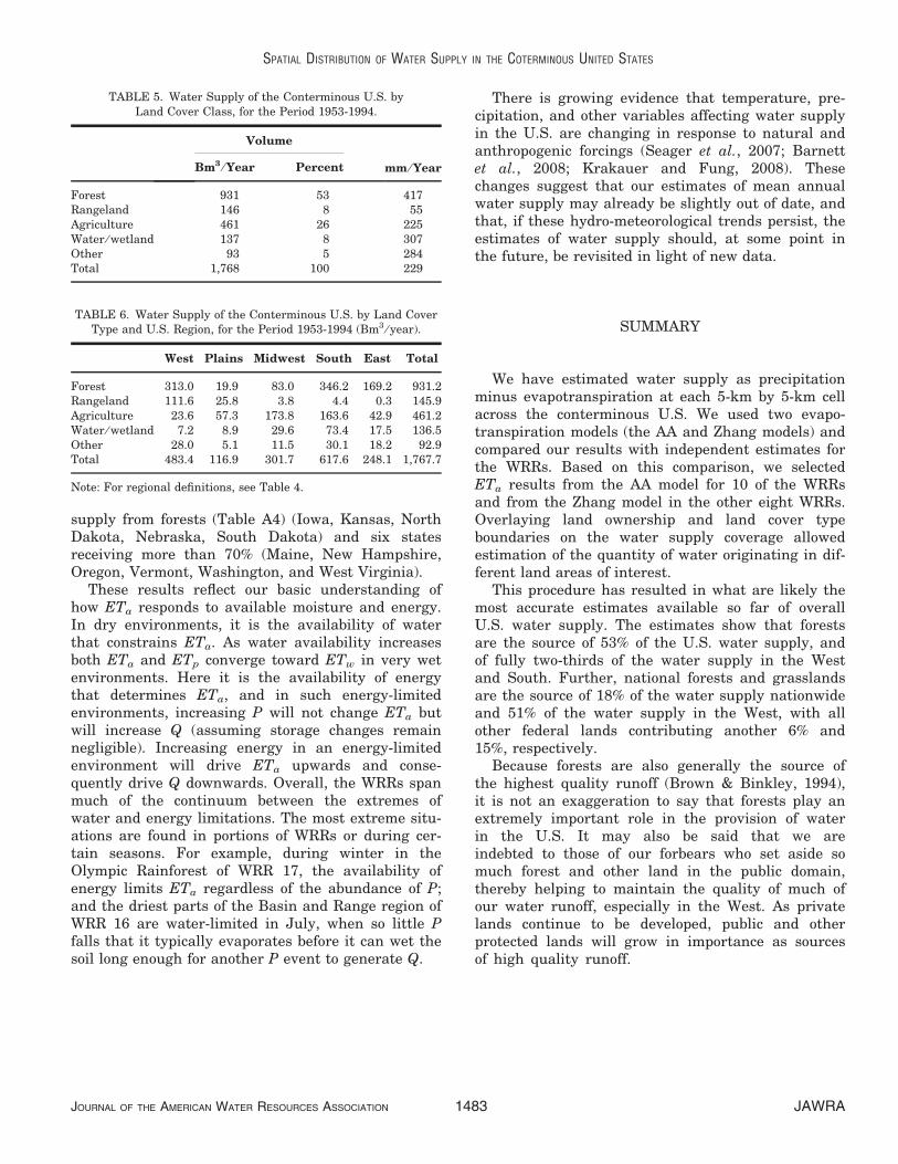
supply from forests (Table A4) (Iowa, Kansas, NorthDakota, Nebraska, South Dakota) and six statesreceiving more than 70% (Maine, New Hampshire,Oregon, Vermont, Washington, and West Virginia).

These results reflect our basic understanding ofhow ETa responds to available moisture and energy.In dry environments, it is the availability of waterthat constrains ETa. As water availability increasesboth ETa and ETp converge toward ETw in very wetenvironments. Here it is the availability of energythat determines ETa, and in such energy-limitedenvironments, increasing P will not change ETa butwill increase Q (assuming storage changes remainnegligible). Increasing energy in an energy-limitedenvironment will drive ETa upwards and conse-quently drive Q downwards. Overall, the WRRs spanmuch of the continuum between the extremes ofwater and energy limitations. The most extreme situ-ations are found in portions of WRRs or during cer-tain seasons. For example, during winter in theOlympic Rainforest of WRR 17, the availability ofenergy limits ETa regardless of the abundance of P;and the driest parts of the Basin and Range region ofWRR 16 are water-limited in July, when so little Pfalls that it typically evaporates before it can wet thesoil long enough for another P event to generate Q.

There is growing evidence that temperature, pre-cipitation, and other variables affecting water supplyin the U.S. are changing in response to natural andanthropogenic forcings (Seager et al., 2007; Barnettet al., 2008; Krakauer and Fung, 2008). Thesechanges suggest that our estimates of mean annualwater supply may already be slightly out of date, andthat, if these hydro-meteorological trends persist, theestimates of water supply should, at some point inthe future, be revisited in light of new data.

SUMMARY

We have estimated water supply as precipitationminus evapotranspiration at each 5-km by 5-km cellacross the conterminous U.S. We used two evapo-transpiration models (the AA and Zhang models) andcompared our results with independent estimates forthe WRRs. Based on this comparison, we selectedETa results from the AA model for 10 of the WRRsand from the Zhang model in the other eight WRRs.Overlaying land ownership and land cover typeboundaries on the water supply coverage allowedestimation of the quantity of water originating in dif-ferent land areas of interest.

This procedure has resulted in what are likely themost accurate estimates available so far of overallU.S. water supply. The estimates show that forestsare the source of 53% of the U.S. water supply, andof fully two-thirds of the water supply in the Westand South. Further, national forests and grasslandsare the source of 18% of the water supply nationwideand 51% of the water supply in the West, with allother federal lands contributing another 6% and15%, respectively.

Because forests are also generally the source ofthe highest quality runoff (Brown & Binkley, 1994),it is not an exaggeration to say that forests play anextremely important role in the provision of waterin the U.S. It may also be said that we areindebted to those of our forbears who set aside somuch forest and other land in the public domain,thereby helping to maintain the quality of much ofour water runoff, especially in the West. As privatelands continue to be developed, public and otherprotected lands will grow in importance as sourcesof high quality runoff.

TABLE 5. Water Supply of the Conterminous U.S. byLand Cover Class, for the Period 1953-1994.

Volume

mm ⁄ YearBm3 ⁄ Year Percent

Forest 931 53 417Rangeland 146 8 55Agriculture 461 26 225Water ⁄ wetland 137 8 307Other 93 5 284Total 1,768 100 229

TABLE 6. Water Supply of the Conterminous U.S. by Land CoverType and U.S. Region, for the Period 1953-1994 (Bm3 ⁄ year).

West Plains Midwest South East Total

Forest 313.0 19.9 83.0 346.2 169.2 931.2Rangeland 111.6 25.8 3.8 4.4 0.3 145.9Agriculture 23.6 57.3 173.8 163.6 42.9 461.2Water ⁄ wetland 7.2 8.9 29.6 73.4 17.5 136.5Other 28.0 5.1 11.5 30.1 18.2 92.9Total 483.4 116.9 301.7 617.6 248.1 1,767.7

Note: For regional definitions, see Table 4.



APPENDIX

The following four tables of mean annual water supply (Q) estimates are based on the Mixed model for theperiod 1953-1994.

TABLE A1. Water Supply (Mm3 ⁄ year) of the Conterminous U.S. by Land Ownership.

WRR NFS BLM NPS BIA Other Federal State & Private Total

1 3,889 0 80 79 443 89,148 93,6402 4,703 0 738 0 993 118,101 124,5343 15,901 0 454 137 6,369 251,861 274,7214 8,717 0 134 960 699 89,010 99,5205 14,914 0 556 68 2,048 168,966 186,5516 12,351 0 1,882 170 1,939 46,657 62,9997 2,360 0 150 592 771 104,932 108,8048 5,499 0 55 1 2,468 117,344 125,3679 1,288 0 109 757 73 7,533 9,760

10 17,791 1,931 4,537 3,104 721 70,550 98,63511 8,999 77 260 867 2,007 76,574 88,78312 2,296 2 138 3 876 46,605 49,92013 3,982 263 32 283 75 2,009 6,64314 14,652 2,225 185 311 51 3,383 20,80615 3,037 476 119 949 37 1,120 5,73816 8,121 2,772 84 33 118 2,605 13,73417 154,591 12,954 20,748 6,724 3,024 105,113 303,15418 42,601 5,313 6,066 978 1,712 38,536 95,207Total 325,691 26,013 36,326 16,018 24,423 1,340,045 1,768,516

Note: Mm3, million cubic meters.

TABLE A2. Water Supply (Mm3 ⁄ year) of the Conterminous U.S. by State and Land Ownership.

State NFS BLM NPS BIA Other Federal State & Private Total

AL 2,852 0 45 0 902 66,615 70,414AR 6,170 0 128 0 1,263 51,323 58,884AZ 2,517 213 93 949 35 902 4,709CA 43,317 5,096 5,878 978 1,568 36,210 93,047CO 15,384 1,509 478 107 75 5,006 22,559CT 0 0 0 0 10 7,683 7,693DC 0 0 6 0 3 72 81DE 0 0 0 0 39 1,950 1,989FL 2,149 0 303 103 1,982 39,930 44,467GA 5,329 0 53 0 1,676 52,870 59,928IA 0 0 1 4 153 31,141 31,299ID 41,372 3,498 131 1,755 297 14,011 61,064IL 1,451 0 0 0 272 38,347 40,070IN 1,005 0 9 0 378 30,345 31,736KS 0 0 7 92 218 16,147 16,464KY 4,183 0 204 0 874 44,123 49,384LA 1,713 0 38 1 1,379 52,485 55,616MA 2 0 22 0 142 11,922 12,088MD 0 0 80 0 146 9,393 9,619ME 199 0 65 79 184 50,343 50,870MI 6,569 0 76 289 392 39,560 46,886MN 2,505 0 173 1,145 164 23,839 27,826MO 3,490 0 130 0 458 46,642 50,720MS 5,303 0 7 35 828 59,060 65,232MT 29,805 1,084 4,057 2,855 234 10,584 48,620NC 8,825 0 1,031 170 1,180 43,123 54,329ND 84 1 3 78 51 3,871 4,088NE 47 0 8 155 51 11,239 11,500



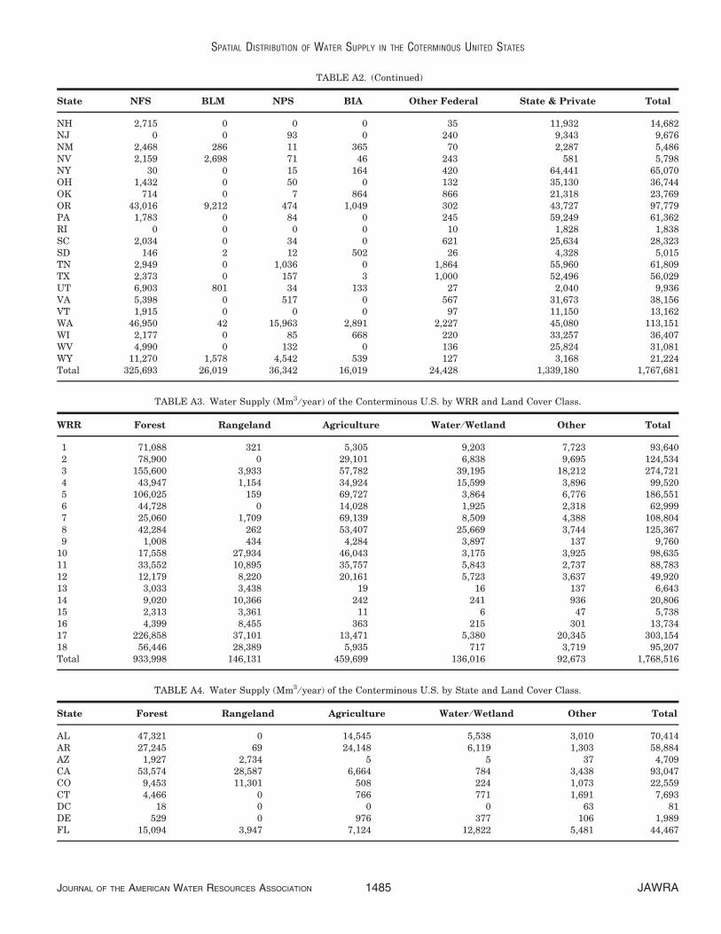
TABLE A2. (Continued)

State NFS BLM NPS BIA Other Federal State & Private Total

NH 2,715 0 0 0 35 11,932 14,682NJ 0 0 93 0 240 9,343 9,676NM 2,468 286 11 365 70 2,287 5,486NV 2,159 2,698 71 46 243 581 5,798NY 30 0 15 164 420 64,441 65,070OH 1,432 0 50 0 132 35,130 36,744OK 714 0 7 864 866 21,318 23,769OR 43,016 9,212 474 1,049 302 43,727 97,779PA 1,783 0 84 0 245 59,249 61,362RI 0 0 0 0 10 1,828 1,838SC 2,034 0 34 0 621 25,634 28,323SD 146 2 12 502 26 4,328 5,015TN 2,949 0 1,036 0 1,864 55,960 61,809TX 2,373 0 157 3 1,000 52,496 56,029UT 6,903 801 34 133 27 2,040 9,936VA 5,398 0 517 0 567 31,673 38,156VT 1,915 0 0 0 97 11,150 13,162WA 46,950 42 15,963 2,891 2,227 45,080 113,151WI 2,177 0 85 668 220 33,257 36,407WV 4,990 0 132 0 136 25,824 31,081WY 11,270 1,578 4,542 539 127 3,168 21,224Total 325,693 26,019 36,342 16,019 24,428 1,339,180 1,767,681

TABLE A3. Water Supply (Mm3 ⁄ year) of the Conterminous U.S. by WRR and Land Cover Class.

WRR Forest Rangeland Agriculture Water ⁄ Wetland Other Total

1 71,088 321 5,305 9,203 7,723 93,6402 78,900 0 29,101 6,838 9,695 124,5343 155,600 3,933 57,782 39,195 18,212 274,7214 43,947 1,154 34,924 15,599 3,896 99,5205 106,025 159 69,727 3,864 6,776 186,5516 44,728 0 14,028 1,925 2,318 62,9997 25,060 1,709 69,139 8,509 4,388 108,8048 42,284 262 53,407 25,669 3,744 125,3679 1,008 434 4,284 3,897 137 9,760

10 17,558 27,934 46,043 3,175 3,925 98,63511 33,552 10,895 35,757 5,843 2,737 88,78312 12,179 8,220 20,161 5,723 3,637 49,92013 3,033 3,438 19 16 137 6,64314 9,020 10,366 242 241 936 20,80615 2,313 3,361 11 6 47 5,73816 4,399 8,455 363 215 301 13,73417 226,858 37,101 13,471 5,380 20,345 303,15418 56,446 28,389 5,935 717 3,719 95,207Total 933,998 146,131 459,699 136,016 92,673 1,768,516

TABLE A4. Water Supply (Mm3 ⁄ year) of the Conterminous U.S. by State and Land Cover Class.

State Forest Rangeland Agriculture Water ⁄ Wetland Other Total

AL 47,321 0 14,545 5,538 3,010 70,414AR 27,245 69 24,148 6,119 1,303 58,884AZ 1,927 2,734 5 5 37 4,709CA 53,574 28,587 6,664 784 3,438 93,047CO 9,453 11,301 508 224 1,073 22,559CT 4,466 0 766 771 1,691 7,693DC 18 0 0 0 63 81DE 529 0 976 377 106 1,989FL 15,094 3,947 7,124 12,822 5,481 44,467



TABLE A4. (Continued)

State Forest Rangeland Agriculture Water ⁄ Wetland Other Total

GA 35,955 116 13,252 6,133 4,472 59,928IA 2,393 1,772 25,327 863 945 31,299ID 38,182 15,756 3,506 863 2,758 61,064IL 5,691 326 29,864 2,005 2,184 40,070IN 6,442 135 22,887 999 1,273 31,736KS 378 5,283 9,834 579 390 16,464KY 29,720 0 16,728 1,613 1,323 49,384LA 18,217 278 17,182 17,506 2,434 55,616MA 7,375 16 643 1,508 2,546 12,088MD 4,087 0 3,732 971 829 9,619ME 40,569 291 2,411 5,318 2,281 50,870MI 19,776 1,004 14,723 9,701 1,681 46,886MN 6,346 203 12,477 7,995 805 27,826MO 14,842 209 31,852 2,274 1,542 50,720MS 32,512 10 21,885 8,506 2,320 65,232MT 27,805 15,167 2,509 546 2,593 48,620NC 34,087 0 11,540 6,122 2,580 54,329ND 9 951 2,899 200 30 4,088NE 16 3,769 7,178 366 171 11,500NH 12,072 0 768 1,107 735 14,682NJ 4,214 0 1,852 1,383 2,226 9,676NM 2,537 2,826 74 11 38 5,486NV 998 4,582 34 35 149 5,798NY 43,133 0 14,240 3,944 3,754 65,070OH 12,748 8 20,691 1,082 2,214 36,744OK 6,388 5,887 9,429 1,361 704 23,769OR 78,293 7,899 6,679 977 3,931 97,779PA 41,310 0 15,707 1,107 3,237 61,362RI 1,198 0 53 242 345 1,838SC 15,671 0 6,336 4,275 2,041 28,323SD 51 923 3,736 266 40 5,015TN 38,059 0 18,392 2,663 2,695 61,809TX 13,023 8,945 24,202 6,101 3,758 56,029UT 4,261 5,061 178 111 325 9,936VA 25,743 0 8,817 1,876 1,719 38,156VT 10,203 13 1,799 773 374 13,162WA 87,885 7,695 3,032 2,898 11,641 113,151WI 14,760 155 15,944 4,659 889 36,407WV 26,548 0 3,639 195 700 31,081WY 8,077 10,009 391 730 2,017 21,224Total 931,202 145,925 461,156 136,504 92,893 1,767,681

LITERATURE CITED

Barnett, T.P., D.W. Pierce, H.G. Hidalgo, C. Bonfils, B.D. Santer,T. Das, G. Bala, A.W. Wood, T. Nozawa, A.A. Mirin, D.R. Cayanand M.D. Dettinger, 2008. Human-Induced Changes in theHydrology of the Western United States. Science 319(5866):1080-1083.

Bouchet, R.J., 1963. Evapotranspiration Reelle EvapotranspirationPotentielle, Signification Climatique. International Associationof Scientific Hydrology, Berkeley, California.

Brown, T.C. and D. Binkley, 1994. Effect of Management on WaterQuality in North American Forests. General Technical ReportRM-248. Rocky Mountain Forest and Range Experiment Sta-tion, Fort Collins, Colorado.

Brutsaert, W. and H. Stricker, 1979. An Advection-AridityApproach to Estimate Actual Regional Evapotranspiration.Water Resources Research 15(2):443-450.

Daly, C., R.P. Neilson, and D.L. Phillips, 1994. A Statistical-Topographic Model for Mapping Climatological Precipitationover Mountainous Terrain. Journal of Applied Meteorology33(2):140-158.

EarthInfo, 1998a. NCDC Summary of the Day [TD-3200 ComputerFile]. EarthInfo, Inc., Boulder, Colorado.

EarthInfo, 1998b. NCDC Surface Airways [TD-3280 ComputerFile]. EarthInfo, Inc., Boulder, Colorado.

Foxworthy, B.L. and D.W. Moody, 1986. National Perspective onSurface-Water Resources. In: National Water Summary 1985 –Hydrologic Events and Surface-Water Resources, Water SupplyPaper 2300, D.W. Moody, E.B. Chase, and D.A. Aronson(Editors). U. S. Geological Survey, Washington, D.C., pp. 51-68.

Graczyk, D.J., W.R. Krug, and W.A. Gebert, 1986. A History ofAnnual Streamflows from the 21 Water-Resource Regions in theUnited States and Puerto Rico, 1951-83. Open-File Report86-128. U.S. Geological Survey, Madison, Wisconsin.



Gutman, G., 1988. A Simple Method for Estimating Monthly MeanAlbedo from AVHRR Data. Journal of Applied Meteorology27(9):973-988.

Hobbins, M.T., J.A. Ramirez, and T.C. Brown, 2001a. The Comple-mentary Relationship in Estimation of Regional Evapotranspi-ration: An Enhanced Advection-Aridity Model. Water ResourcesResearch 37(5):1389-1403.

Hobbins, M.T., J.A. Ramirez, and T.C. Brown, 2004a. Developing aLong-Term, High-Resolution, Continental-Scale, Spatially Dis-tributed Time-Series of Topographically Corrected Solar Radia-tion. Proceedings of the Twenty-fourth Annual AmericanGeophysical Union Hydrology Days, Colorado State University,Fort Collins, Colorado.

Hobbins, M.T., J.A. Ramirez, and T.C. Brown, 2004b. Trends inPan Evaporation and Actual Evaporation Across the Contermi-nous U.S.: Paradoxical or Complementary? GeophysicalResearch Letters 31(13):L13503.

Hobbins, M.T., J.A. Ramirez, T.C. Brown, and L.H.J.M. Claessens,2001b. The Complementary Relationship in Estimation of Regio-nal Evapotranspiration: The Complementary Relationship ArealEvapotranspiration and Advection-Aridity Models. WaterResources Research 37(5):1367-1387.

Hydrosphere Data Products, 1996. Hydrodata USGS Daily Values,Volume 8.0. Hydrosphere Data Products, Inc., Boulder, Colo-rado.

Krakauer, N.Y. and I. Fung, 2008. Is Streamflow Increasing?Trends in the Coterminous United States. Hydrology and EarthSystem Sciences Discussions 5(2):785-810.

Mooty, W.B. and H.H. Jeffcoat, 1986. Inventory of InterbasinTransfers of Water in the Eastern United States. Open-FileReport 86-148. U.S. Geological Survey, Tuscaloosa, Alabama.

Morton, F.I., 1983. Operational Estimates of Areal Evapotranspira-tion and Their Significance to the Science and Practice ofHydrology. Journal of Hydrology 66:1-76.

National Climatic Data Center (NCDC), 1993. Solar and Meteoro-logical Surface Observation Network 1961-1990 (CD-ROM), Ver-sion 1.0. National Climatic Data Center, Asheville, NorthCarolina.

National Climatic Data Center (NCDC), 2001. Solmet [TD9724Computer File] Solar and Surface Observations, Daily 1952-1976, Solmet Volume 1 - User’s Manual TD-9724. National Cli-matic Data Center, Boulder, Colorado.

National Climatic Data Center (NCDC), 2004a. Surface Airways,TD3280. National Climatic Data Center, Asheville, North Caro-lina.

National Climatic Data Center (NCDC), 2004b. Surface Land DailyCooperative Summary of the Day, TD-3200. National ClimaticData Center., Asheville, North Carolina.

Oliver, M.A. and R. Webster, 1990. Kriging: A Method ofInterpolation for Geographical Information Systems.International Journal of Geographical Information Science4(3):313-332.

Penman, H.L., 1948. Natural Evaporation From Open Water, BareSoil and Grass. Proceedings of the Royal Society of London,London.

Petsch, H.E. Jr., 1985. Inventory of Interbasin Transfers of Waterin the Western Conterminous United States. Open-File Report85-166. U.S. Geological Survey, Lakewood, Colorado.

Priestley, C.H.B. and R.J. Taylor, 1972. On the Assessment of Sur-face Heat Flux and Evaporation Using Large-Scale Parameters.Monthly Weather Review 100:81-92.

Public Land Law Review Commission, 1970. One Third of theNation’s Land: A Report to the President and to the Congressby the Public Land Law Review Commission. Public Land LawReview Commission, Washington, D.C.

Ramirez, J.A., M.T. Hobbins, and T.C. Brown, 2005. ObservationalEvidence of the Complementary Relationship in Regional Evap-

oration Lends Strong Support for Bouchet’s Hypothesis. Geo-physical Research Letters 32(15):L15401.

Seager, R., M.F. Ting, I. Held, Y. Kushnir, J. Lu, G. Vecchi, H-P.Huang, N. Harnik, A. Leetmaa, N-C. Lau, C. Li, J. Velez and N.Naik, 2007. Model Projections of an Imminent Transition to aMore Arid Climate in Southwestern North America. Science316(5828):1181-1184.

Sedell, J., M. Sharpe, D.D. Apple, M. Copenhagen, and M. Furniss,2000. Water and the Forest Service. U.S. Forest Service, Wash-ington, D.C.

Slack, J.R. and J.M. Landwehr, 1992. Hydro-Climatic Data Net-work (HCDN): A U. S. Geological Survey Streamflow Data Setfor the United States for the Study of Climate Variations, 1874-1988. Open-File Report 92-129. U. S. Geologic Survey, Reston,VA.

Szilagyi, J., 2001. On Bouchet’s Complementary Hypothesis. Jour-nal of Hydrology 246(1-4):155-158.

U.S. Geological Survey, 1992. National Land Cover Data Set(Updated). U.S. Department of Interior, Reston, Virginia (http://landcover.usgs.gov/natlandcover.asp).

U.S. Geological Survey, 2004. Federal Lands of the United States:National Atlas of the United States. 200412. U.S. Departmentof Interior, Reston, Virginia (http://nationalatlas.gov/atlasftp.html).

U.S. Water Resources Council, 1978. The Nation’s Water Resources1975-2000. Government Printing Office, Washington, D.C.

Zhang, L., W.R. Dawes, and G.R. Walker, 2001. Response of MeanAnnual Evapotranspiration to Vegetation Changes at Catch-ment Scale. Water Resources Research 37(3):701-708.



Documents

SPATIAL DISTRIBUTION OF WATER SUPPLY IN THE … · SPATIAL DISTRIBUTION OF WATER SUPPLY IN THE COTERMINOUS UNITED STATES1 ... Spatial Distribution of Water Supply in ... and dries