Space Mapping and Defect Correction - Stanford Universitypangea.stanford.edu/~echeverr/sfcpapers/chapter00.pdf · Space Mapping and Defect Correction ... (the ‘Aggressive Space

Space Mapping and Defect Correction

David Echeverrıa, Domenico Lahaye, and Piet W. Hemker

CWI, Kruislaan 413, 1054 AL Amsterdam, The Netherlands∗∗

{D.Echeverria,P.W.Hemker,Domenico.Lahaye}@cwi.nl

Summary. In this chapter we present the principles of the space-mapping iteration techniquesfor the efficient solution of optimization problems. We also show how space-mapping opti-mization can be understood in the framework of defect correction.

We observe the difference between the solution of the optimization problem and the com-puted space-mapping solutions. We repair this discrepancy by exploiting the correspondencewith defect correction iteration and we construct the manifold-mapping algorithm, which is asefficient as the space-mapping algorithm but converges to the true solution.

In the last section we show a simple example from practice, comparing space-mappingand manifold mapping and illustrating the efficiency of the technique.

1 Introduction

Space mapping is a technique, using simple surrogate models, to reduce the com-puting time in optimization procedures where time-consuming computer-models areneeded to obtain sufficiently accurate results. Thus, space mapping makes use ofboth accurate (and time-consuming) models and less accurate (but cheaper) ones.

In fact, the original space-mapping procedure corresponds with right-preconditioning the coarse (inaccurate) model in order to accelerate the iterativeprocedure for the optimization of the fine (accurate) one. The iterative procedureused in space mapping for optimization can be seen as a defect correction iterationand the convergence can be analyzed accordingly. In this paper we show the struc-ture of space mapping iteration. We also show that right-preconditioning is generallyinsufficient and (also) left-preconditioning is needed to obtain the solution for theaccurate model. This leads to the improved space-mapping or ‘manifold-mapping’procedure. This manifold mapping is shown in some detail in Section 5 and in thelast section a few examples of an application are given.

The space-mapping idea was introduced by Bandler [3] in the context ofmicrowave filter design and it has developed significantly over the last decade. In the

∗∗ This research was supported by the Dutch Ministry of Economic Affairs through the projectIOP-EMVT-02201 B

158 D. Echeverrıa et al.

rather complete survey [4] we see that the original idea has gone through a largenumber of changes and improvements. The reader is referred to the original litera-ture [1, 2, 5] for a review of earlier achievements and for a classical introduction forengineers.

2 Fine and Coarse Models in Optimization

The Optimization Problem.

Let the specifications for the data of an optimization problem be denoted by (t,y) ≡({ti}, {yi})i=1,...,m. The independent variable t ∈ R

m could be, e.g., time, fre-quency, space, etc. The dependent variable y ∈ Y ⊂ R

m represents the quantitiesthat describe the behavior of the phenomena under study or design. The set Y ⊂ R

m

is called the set of possible aims.The behavior of the variable y not only depends on the independent variable t

but also on an additional set of control/design variables. With x the vector of relevantcontrol variables, we may write the components of y as yi ≈ y(ti,x). The behaviorof the phenomenon is described by the function y(t,x) and the difference betweenthe measured data yi and the values y(ti,x) may be the result of, e.g., measurementerrors or the imperfection of the mathematical description.

Models to describe reality appear in several degrees of sophistication. Spacemapping exploits the combination of the simplicity of the less sophisticated methodswith the accuracy of the more complex ones. Therefore, we distinguish two types ofmodel: fine and coarse.

The Fine Model.

The fine model response is denoted by f(x) ∈ Rm, where x ∈ X ⊂ R

n is the finemodel control variable. The set X of possible control variables is usually a closedand bounded subset of R

n. The set f(X) ⊂ Rm of all possible fine model responses

is the set of fine model reachable aims. The fine model is assumed to be accurate butexpensive to evaluate. We also assume that f(x) is continuous.

For the optimization problem a fine model cost function, ||| f(x)−y||| , is defined,which is a measure for the discrepancy between the data and a particular response ofthe mathematical model. This cost function should be minimized. So we look for

x∗ = argminx∈X

||| f(x) − y||| . (1)

A design problem, characterized by the model f(x), the aim y ∈ Y , and the spaceof possible controls X ⊂ R

n, is called a reachable design if the equality f(x∗) = ycan be achieved for some x∗ ∈ X . �

Space Mapping and Defect Correction 159

The Coarse Model.

The coarse model is denoted by c(z) ∈ Rm, with z ∈ Z ⊂ R

n the coarse modelcontrol variable. This model is assumed to be cheap to evaluate but less accuratethan the fine model. The set c(Z) ⊂ R

m is the set of coarse model reachable aims.For the coarse model we have the coarse model cost function, ||| c(z)−y||| . We denoteits minimizer by z∗,

z∗ = argminz∈Z

||| c(z) − y||| . (2)

We assume that the fine and coarse optimization problems, characterized by y,f(x) and X , respectively y, c(z) and Z, are uniquely solvable and well defined.If X and Z are closed and bounded non-empty sets in R

n and f and c continuousfunctions, the existence of the solutions is guaranteed. Generally, uniqueness can beachieved by properly reducing the sets X or Z. If the models are non-injective (orextremely ill-conditioned) in a small neighborhood of a solution, essential difficultiesmay arise.

The Space-Mapping Function.

The similarity or discrepancy between the responses of two models used for the samephenomenon is an important property. It is expressed by the misalignment function

r(z,x) = ||| c(z) − f(x)||| . (3)

For a given x ∈ X it is useful to know which z ∈ Z yields the smallest discrep-ancy. This information can be used to improve the coarse model. Therefore, thespace-mapping function is introduced. The space-mapping function p : X ⊂ R

n →Z ⊂ R

n is defined1 by

p(x) = argminz∈Z

r(z,x) = argminz∈Z

||| c(z) − f(x)||| . (4)

It should be noted that this evaluation of the space-mapping function p(x) re-quires both an evaluation of f(x) and a minimization process with respect to zin ||| c(z) − f(x)||| . Hence, in algorithms we should make economic use of space-mapping function evaluations. In Figure 1 we see an example of a misalignmentfunction and of a few space mapping functions.

Perfect Mapping.

In order to identify the cases where the accurate solution x∗ is related with the lessaccurate solution z∗ by the space mapping function, the following definition is intro-duced. A space-mapping function p is called a perfect mapping iff

1 The process of finding p(x) for a given x is called parameter extraction or single pointextraction because it finds the best coarse-model parameter that corresponds with a givenfine-model control x.


z (m

m)

x (mm)2 3 4 5 6 7 8

2

3

4

5

6

7

8

2 3 4 5 6 7 82

3

4

5

6

7

8

z (m

m)

x (mm)

LinearNonlinear,σ =1.0Nonlinear,σ = 1.4Identity

Fig. 1. Misalignment and space-mapping function

The left figure shows the misalignment function for a fine and a coarse model. Darker shadingshows a smaller misalignment. The right figure shows the identity function and a few space-mapping functions for different coarse models (example taken from [9]).

z∗ = p(x∗) . (5)

Using the definition of space mapping we see that (5) can be written as

argminz∈Z

||| c(z) − y||| = argminz∈Z

||| c(z) − f(x∗)||| , (6)

i.e., a perfect space-mapping function maps x∗, the solution of the fine modeloptimization, exactly onto z∗, the minimizer of the coarse model design.

Remark. We notice that perfection is not only a property of the space-mapping func-tion, but it also depends on the data y considered. A space-mapping function can beperfect for one set of data but imperfect for a different data set. In this sense ‘perfectmapping’ can be a confusing notion.

3 Space-Mapping Optimization

In literature many space mapping based algorithms can be found [1, 4], but theyall have the same basis. We first describe the original space-mapping idea and theresulting two principal approaches (primal and dual).

3.1 Primal and Dual Space-Mapping Solutions

The idea behind space-mapping optimization is the following: if either the fine modelallows for an almost reachable design (i.e., f(x∗) ≈ y) or if both models are similarnear their respective optima (i.e., f(x∗) ≈ c(z∗)), we expect


p(x∗) = argminz∈Z

||| c(z) − f(x∗)||| ≈ argminz∈Z

||| c(z) − y||| = z∗ . (7)

Based on this relation, the space-mapping approach assumes p(x∗) ≈ z∗. However,in general p(x∗) �= z∗ and even z∗ ∈ p(X) is not guaranteed. Therefore the primalspace-mapping approach seeks for a solution of the minimization problem

x∗p = argmin

x∈X‖p(x) − z∗‖ . (8)

An alternative approach can be chosen. The idea behind space-mapping opti-mization is the replacement of the expensive fine model optimization by a surrogatemodel. For the surrogate model we can take the coarse model c(z), and improve itsaccuracy by the space mapping function p. Now the improved or mapped coarsemodel c(p(x)) may serve as the better surrogate model. Because of (4) we expectc(p(x)) ≈ f(x) and hence ||| f(x) − y||| ≈ ||| c(p(x)) − y||| . Then the minimizationof ||| c(p(x))−y||| will usually give us a value, x∗

d, close to the desired optimum x∗:

x∗d = argmin

x∈X||| c(p(x)) − y||| . (9)

This is the dual space-mapping approach.We will see in Section 3.3 that both approaches coincide when z∗ ∈ p(X) and

p is injective, and if the mapping is perfect both x∗p and x∗

d are equal to x∗. However,in general the space-mapping function p will not be perfect, and hence, a spacemapping based algorithm will not yield the solution of the fine model optimization.The principle of the approach is summarized in Figure 2.

Fig. 2. Diagram showing the main idea of space mapping


x0 = z∗ = argminz∈Z ||| c(z) − y|||B0 = Ifor k = 0, 1, . . .while |||p(xk) − z∗||| > tolerancedohk = −B−1

k (p(xk) − z∗)xk+1 = xk + hk

Bk+1 = Bk +(p(xk+1)−z∗)hT

hT h

enddo

Fig. 3. The ASM algorithm

3.2 Space-Mapping Algorithms

Because the evaluation of the space-mapping function is expensive, algorithms tocompute x∗

p or x∗d are based on iterative approximation of p(x). By the similarity of

f(x) and c(z), a first approximation is the identity, p0 = I .Linear approximations form the basis for the more popular space-mapping opti-

mization algorithms. An extensive survey of available algorithms can be found in [4].The most representative example is ASM (the ‘Aggressive Space Mapping’ shownin Figure 3), where the space-mapping function is approximated by linearisation toobtain

pk(x) = p(xk) + Bk (x − xk) . (10)

In each space-mapping iteration step the matrix Bk is adapted by a rank-one up-date. For that purpose a Broyden-type approximation for the Jacobian of the space-mapping function p(x) is used,

Bk+1 = Bk +p(xk+1) − p(xk) − Bkh

hT hhT , (11)

where h = xk+1 − xk. This is combined with original space mapping, so thatxk+1 = xk − B−1

k (p(xk) − z∗).

3.3 Perfect Mapping, Flexibility and Reachability

By its definition, perfect mapping relates the similarity of the models and the specifi-cations. If the fine model allows for a reachable design, then it is immediate that, in-dependent of the coarse model used, the mapping is always perfect. Also if the coarseand the fine model optimal responses are identical, the space-mapping function isperfect. These two facts are summarized in the following lemma.

Lemma 1. (i) If f(x∗) = y then p(x∗) = z∗;(ii) If f(x∗) = c(z∗) then p(x∗) = z∗.

The following lemma [9] follows from the definitions (8) and (9).

Lemma 2. (i) If z∗ ∈ p(X), then p(x∗p) = p(x∗

d) = z∗;(ii) If, in addition, p is an injective perfect mapping then x∗ = x∗

p = x∗d.


In some cases we can expect that the sets of fine and coarse reachable aimsoverlap in a region of R

m close to their respective optima. The concept of model flex-ibility is introduced and from that some results concerning properties of the space-mapping functions can be derived.

Definition 1. A model is called more flexible than another if the set of its reachableaims contains the set of reachable aims of the other. Two models are equally flexibleif their sets of reachable aims coincide. �

Thus, a coarse model c is more flexible than the fine one f if c(Z) ⊃ f(X), i.e., if thecoarse model response can reproduce all the fine model reachable aims. Similarly thefine model is more flexible if f(X) ⊃ c(Z). Model flexibility is closely related toproperties of the space-mapping function. This is shown in the following lemmas,where p denotes the space-mapping function. Proofs are found in [9].

Lemma 3. If c is more flexible than f then(i) c(p(x)) = f(x) ∀x ∈ X;(ii) p : X → Z is a perfect mapping ⇔ c(z∗) = f(x∗);(iii) if f : X → Y is injective then p : X → Z is injective;(iv) if c(Z) \ f(X) �= ∅, then p : X → Z cannot be surjective.

Remark. Because of (ii) generally we cannot expect space-mapping functions to beperfect for flexible coarse models unless the two models are equally flexible near theoptimum. However, we remind that if the design is reachable, the perfect mappingproperty holds, even if c(Z) \ f(X) �= ∅.

Lemma 4. If f is more flexible than c then(i) p : X → Z is surjective;(ii) if f(X) \ c(Z) �= ∅, then p cannot be injective.

We combine the previous two lemmas in the following.

Lemma 5. If f and c are equally flexible and f : X → Y is injective, then (i) p is abijection, and (ii) p is a perfect mapping.

The conclusions in Lemma 2 can now be derived from assumptions about modelflexibility.

Lemma 6. (i) If f is more flexible than c, then p(x∗p) = p(x∗

d) = z∗. (ii) If f and care equally flexible and f is injective, then x∗ = x∗

p = x∗d.

Remark. It is not really needed for the space-mapping function to be a bijectionover the whole domain in which it is defined. In fact, perfect mapping is a propertythat concerns only a point, and it is enough if the function is injective in a (small)neighborhood. Thus the assumptions for the former lemmas can be relaxed and statedjust locally.


4 Defect Correction and Space Mapping

The technique underlying space-mapping, i.e. the efficient solution of a complexproblem by the iterative use of a simpler one, is known since long in computationalmathematics. In numerical analysis it is known as defect correction iteration andstudied in a number of papers [6, 7]. Below we first briefly summarize the defectcorrection principle for solving operator equations and then we apply the idea tooptimization problems.

4.1 Defect Correction for Operator Equations

We first consider the problem of solving a nonlinear operator equation

F x = y, (12)

where F : D ⊂ E → D ⊂ E is a continuous, generally nonlinear operator andE and E are Banach spaces. In general, neither injectivity nor surjectivity of themapping is assumed, but in many cases these properties can be achieved by a properchoice of the subsets D and D.

The classical defect correction iteration for the solution of equation (12) withy ∈ F(D) ⊂ D is based on a sequence of operators Fk : D → D approximating F .We assume that each Fk has an easy-to-calculate inverse Gk : D → D. Actually, itis the existence of the easy-to-evaluate operator Gk, rather than the existence of Fk,that is needed for defect correction and we do not need to assume Gk to be invertible.

Defect correction comes in two brands [6], depending on the space, E or E, inwhich linear combinations for extrapolation are made. The two basic iterative defectcorrection procedures to generate a (hopefully convergent) sequence of approxima-tions to the solution of (12) are{

x0 = G0 yxk+1 = (I − Gk+1 F)xk + Gk+1 y

and

{l0 = ylk+1 = (I −F Gk) lk + y .

(13)

In the second, (13b), we identify the approximate solution as xk ≡ Gklk. We see thatthe two iteration processes are dual in the sense that in the first, (13a), the extrapo-lation is in the space D, whereas the additions in (13b) are in D. If Gk is injective,then an operator Fk exists such that FkGk = ID, i.e., Fk is the left-inverse of Gk.Then Fkxk = lk and (13b) is equivalent with the iterative procedure{

F0x0 = y ,Fk+1xk+1 = Fk xk − FGkFk xk + y .

(14)

In order to apply (14), the injectivity of Gk is not really needed and it is immedi-ately seen that neither (13b) nor (14) converges if y �∈ F(D). However, (14) can bemodified so that it can be used for y �∈ F(D). Then we need injectivity for Fk andwe take Gk its left-inverse, i.e., GkFk = ID. Then (14) leads to


F not surjective → left-inverse G : GF = ID

Fig. 4. The non-surjective operator in the optimization problem

{x0 = G0 y ,

xk+1 = Gk+1

(Fk xk − F xk + y

).

(15)

Because (15) allows for a non-injective Gk, this iteration can be used for optimizationpurposes. In case of an invertible Gk+1 both (14) and (15) are equivalent with (13b).

For our optimization problems, where the design may be not reachable, y ∈ D,but y /∈ F(D), i.e., F is no surjection so that no solution for (12) exists and (13b)-(14) cannot converge (Figure 4). Therefore, we drop the idea of finding an x ∈ Dsatisfying (12) and we replace the aim by looking for a solution x∗ ∈ D so that thedistance between Fx and y is minimal, i.e., we want to find

x∗ = argminx∈D ‖Fx − y‖E . (16)

For a compact non-empty D and a continuous F , at least a solution exists and ifthe operators Gk are such that (13a) or (15) converges, the stationary point x satisfiesGF x = Gy or x = G(F x − F x + y) respectively. (We assume that Gk = G andFk = F for k large enough.)

Now we can associate with each defect correction iteration a process for iterativeoptimization by taking E = R

n, E = Rm, D = X , D = Y and p : X → Z, and by

substitution of the corresponding operators:

Fx = y ⇔ f(x) = y ,

x = Gy ⇔ x = argminξ

‖f(ξ) − y‖ ,

Fx = y ⇔ c(p(x)) = y ,

x = Gy ⇔ x = argminξ

‖c(p(ξ)) − y‖ .

(17)

Remark. Notice that p is not the space mapping function but an arbitrary (easy tocompute) bijection, e.g., the identity.

4.2 Defect Correction for Optimization

With (17) we derive from (13a) and (15) two defect-correction iteration schemesfor optimization. Substitution of (17) yields the initial estimate and two iterationprocesses for k = 0, 1, 2, · · · , with pk+1 for p in every step,


x0 = argminx∈X

||| c(p0(x)) − y||| , (18)

xk+1 = xk − argminx∈X

||| c(pk+1(x)) − f(xk)|||

+ argminx∈X

||| c(pk+1(x)) − y||| , (19)

xk+1 = argminx∈X

||| c(pk+1(x)) − c(pk(xk)) + f(xk) − y||| . (20)

The two processes (19) and (20) are still dual in the sense that extrapolation is appliedin the space X for process (19) and in Y for process (20). The operators pk are right-preconditioners for the coarse model, which may be adapted during the initial stepsof the iteration. We take pk non-singular and for the initial estimate (18), and ifX = Z we usually take p0 = I , the identity.

In the above iterations every minimization involves the surrogate model, c ◦ pk.However, it is the coarse model that was assumed to be cheaply optimized. Therefore,it is more convenient to write the procedures such that optimization over the coarsemodel becomes obvious. By taking in (13a) and (15) F z = f(q(z)), Fk z = c(z)and Gk y = argminz∈Z ||| c(z)−y||| , with q and qk bijections from Z to X fulfillingin every iteration qzk = qk zk, we obtain, for k = 0, 1, 2, · · · ,

z0 = z∗ = argminz∈Z

||| c(z) − y||| , (21)

zk+1 = zk − argminz∈Z

||| c(z) − f(qk(zk))||| + z∗ , (22)

zk+1 = argminz∈Z

||| c(z) − c(zk) + f(qk(zk)) − y||| . (23)

As the solution is wanted in terms of fine-model control variables, the procedures arecomplemented with xk = qk(zk). The bijections can be interpreted as qk = p−1

k .For k > k0, we assume the iteration process to be stationary: pk = p and qk = q.It is a little exercise to see by proper simplifications of (19) and (20) that space-mapping iteration can be recovered from defect correction [9, Section 4.3.2].

Orthogonality and the Need for Left-preconditioning.

For thestationarypointsof theaboveprocesses,wecanderive the following lemma [9].

Lemma 7. In the case of convergence of (23), with fixed point limk→∞ xk = x weobtain

f(x) − y ∈ c(Z)⊥(p(x)) . (24)

In case of convergence of (22) with a fixed point x we obtain

f(x) − y ∈ c(Z)⊥(z∗) . (25)

Like the space-mapping methods, the above iterations have the disadvantagethat, in general, the fixed point of the iteration does not coincide with the so-lution of the fine model minimization problem. This is due to the fact that the


��

��

��

��

��

�

..........

..........

..........

..........

..........

..........

..........

..........

..........

..........�

......................

......................

............��f(x∗)

� y

� f(x)

c(z∗)c(Z)

f(X)

Fig. 5. The relative location of c(z∗), f(x∗) and f(x)

approximate solution x satisfies either (24) or (25). whereas a (local) minimumx∗ = argminx∈X ‖f(x) − y‖ satisfies (see Figure 5)

f(x∗) − y ∈ f(X)⊥(x∗) . (26)

Hence, differences between x and x∗ will be larger for larger distances betweeny and the sets f(X) and c(Z) and for larger angles between the linear manifoldstangential at c(Z) and f(X) near the optima.

By the orthogonality relations above, we see that it is advantageous, both for theconditioning of the problem and for the minimization of the residual, if the manifoldsf(X) and c(Z) are found parallel in the neighborhood of the solution. However,by space mapping or by right-preconditioning the relation between the manifoldsf(X) and c(Z) remains unchanged. This causes that the fixed point of traditionalspace mapping does generally not correspond with x∗. This relation, however, canbe improved by the introduction of an additional left-preconditioner. Therefore weintroduce such a preconditioner S so that near f(x∗) ∈ Y the manifold c(Z) ⊂ Y ismapped onto f(X) ⊂ Y :

f(x) ≈ S(c(p(x))) . (27)

In the next section we propose a new algorithm where an affine operator maps c(Z)onto f(X) in the neighborhood of the solution. (More precisely: it approximatelymaps one tangential linear manifold onto the other.) This restores the orthogonalityrelation f(x) − y ⊥ f(X)(x∗). Thus it improves significantly the traditional ap-proach and makes the solution x∗ a stationary point of the iteration. Details on theconvergence of the processes can be found in [10].

5 Manifold Mapping, the Improved Space Mapping Algorithm

We introduce the affine mapping S : Y → Y such that Sc(z) = f(x∗) for a properz ∈ Z, and the linear manifold tangential to c(Z) in c(z) maps onto the one tangen-tial to f(X) in f(x∗). Because, in the non-degenerate case when m ≥ n, both f(X)and c(Z) are n-dimensional sets in R

m, the mapping S can be described by


Sv = f(x∗) + S (v − c(z)) , (28)

where S is an m ×m-matrix S of rank n. This mapping S is not a priori available,but an approximation to it can be computed iteratively during the optimization. A fullrank m×m-matrix S can be constructed, which has a well-determined part of rankn, while a remaining part of rank m − n is free to choose. Because of the supposedsimilarity between the models f and c we keep the latter part close to the identity.The meaning of the mapping S is illustrated in the Figures 6 and 7

Fig. 6. Restoring the orthogonality relation by manifold mapping

Better mapping by left and right preconditioning.

Fig. 7. Manifold Mapping


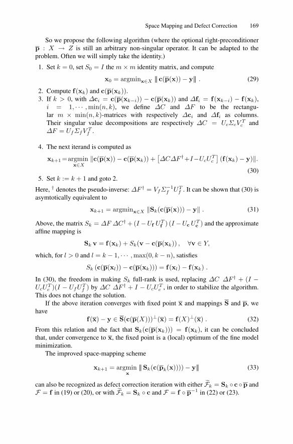
So we propose the following algorithm (where the optional right-preconditionerp : X → Z is still an arbitrary non-singular operator. It can be adapted to theproblem. Often we will simply take the identity.)

1. Set k = 0, set S0 = I the m×m identity matrix, and compute

x0 = argminx∈X ||| c(p(x)) − y||| . (29)

2. Compute f(xk) and c(p(xk)).3. If k > 0, with ∆ci = c(p(xk−i)) − c(p(xk)) and ∆fi = f(xk−i) − f(xk),

i = 1, · · · ,min(n, k), we define ∆C and ∆F to be the rectangu-lar m × min(n, k)-matrices with respectively ∆ci and ∆fi as columns.Their singular value decompositions are respectively ∆C = UcΣcV

Tc and

∆F = UfΣfVTf .

4. The next iterand is computed as

xk+1 =argminx∈X

‖c(p(x)) − c(p(xk)) +[∆C∆F †+I−UcU

Tc

](f(xk) − y)‖.

(30)5. Set k := k + 1 and goto 2.

Here, † denotes the pseudo-inverse: ∆F † = VfΣ−1f UT

f . It can be shown that (30) isasymtotically equivalent to

xk+1 = argminx∈X ‖Sk(c(p(x))) − y‖ . (31)

Above, the matrix Sk = ∆F ∆C† + (I −Uf UTf ) (I −Uc U

Tc ) and the approximate

affine mapping is

Sk v = f(xk) + Sk(v − c(p(xk)) , ∀v ∈ Y,

which, for l > 0 and l = k − 1, · · · ,max(0, k − n), satisfies

Sk (c(p(xl)) − c(p(xk))) = f(xl) − f(xk) .

In (30), the freedom in making Sk full-rank is used, replacing ∆C ∆F † + (I −UcU

Tc )(I − UfU

Tf ) by ∆C ∆F † + I − UcU

Tc , in order to stabilize the algorithm.

This does not change the solution.If the above iteration converges with fixed point x and mappings S and p, we

havef(x) − y ∈ S(c(p(X)))⊥(x) = f(X)⊥(x) . (32)

From this relation and the fact that Sk(c(p(xk))) = f(xk), it can be concludedthat, under convergence to x, the fixed point is a (local) optimum of the fine modelminimization.

The improved space-mapping scheme

xk+1 = argminx

|||Sk(c(pk(x)))) − y||| (33)

can also be recognized as defect correction iteration with either Fk = Sk ◦ c ◦p andF = f in (19) or (20), or with Fk = Sk ◦ c and F = f ◦ p−1 in (22) or (23).


6 Examples

We illustrate the application of space-mapping and manifold-mapping by a designproblem for a linear actuator. We compare the performance of these algorithms withthat of two classical optimization methods: Nelder-Mead Simplex (NMS) and Se-quential Quadratic Programming (SQP).

Linear actuators are electromechanical devices that convert electromechanicalpower into linear motion. An axi-symmetrical variant, called a voice-coil actuator,consisting of a permanent magnet, a current-carrying coil and a ferromagnetic coreis shown in Figure 8. The permanent magnet is magnetized in the vertical direction.The coil, steered by the magnetic force, moves along the z-axis in the gap of thecore, as illustrated in Figure 9. The position of the coil relative to the top of the

Fig. 8. A cylindrical voice-coil actuator consisting of a ferromagnetic core, permanent magnetand coil

Design Variables. Geometry.

Fig. 9. Geometry and design variables of the cylindrical voice-coil actuator


core is denoted by D. Due to the axisymmetrical geometry, the force has an axialcomponent only. It will be denoted by Fz(D).

The design variables [13] are shown in Figure 9: x1 and x2 denote the height andradius of the magnet, x3 and x4 the height and thickness of the coil and x5, x6 andx7 the sizes of the core. Two additional linear inequality constraints define feasiblecoil positions. The air-gap sizes p1 and p2 to the left and right of the coil are keptfixed. Remaining details are found in [11].

We allow the coil to move over a 4 mm range, i.e., 0 ≤ D ≤ 4 mm. The forceon the coil is computed at nine equidistant points Di in this interval. Values for thedesign variables have to be found such that the force response is flat and as close toy = 24 N as possible. The cost function is(

9∑i=1

[Fz(Di) − y(Di)]2/9∑

i=1

y(Di)2)1/2

. (34)

The fine model is a second order Lagrangian finite element (FE) model in whichthe non-linearBH-curve of the ferromagnetic core is taken into account. The force iscomputed by means of the Lorentz Force Law [8]. The number of degrees of freedomin the FE model is between 8000 and 11000, yielding three digits of accuracy in thecomputed force.

The first of two coarse models is a FE model in which the BH-curve of theactuator core is linearized. Depending on the number of Newton iterations requiredin the non-linear case, this model is a factor between 30 and 50 cheaper than the fineone. The second coarse model is a lumped parameter model. This so-called magneticequivalent circuit (MEC) [8] model has a negligible computational cost comparedto the fine one. In both the FE and the MEC coarse models, the relative magneticpermeability in the core was overestimated and set equal to 1000. This was done forillustration purposes.

Below we will consider three variants of modelling approaches for this type ofproblem. The use of manifold mapping with the linearized finite element, respec-tively the MEC as coarse model, will be denoted by FE/MM and MEC/MM. Similarnotations FE/SM and MEC/SM are used for space mapping.

6.1 A Variant with One Design Variable

We initially consider a design problem with a single design variable, only varying theradius of the permanent magnet. We denote the design variable x2 simply by x. Asa starting guess we use the coarse model optimum, i.e., x0 = z∗, as in Section 4.2,where the choice p0 = I was made. For this one-parameter problem both spacemapping (SM) and manifold mapping (MM), with either the linear FE or the MEC ascoarse model, converge to the unique x∗ in four iterations and both methods delivera speed-up with a factor between four and five compared with the NMS or the SQPalgorithm [11].

The cost function associated with the surrogate model that MM builds in thefinal iteration step approximates the fine model cost function in a neighbourhood


x∗ much better than its SM counterpart. We illustrate the convergence of SM andMM by looking at the cost function of the surrogate models during successive itera-tions. Figure 10 (top) shows the cost functions of the surrogate model during the first

Space-Mapping (SM).

Manifold-Mapping (MM).

Fig. 10. Convergence history of SM and MM using the MEC as coarse model


Table 1. Computational efficiency of SM and MM for an example with a single design vari-able, compared with the NMS and the SQP method

# iters # f evals. # c evalsNMS 10 20 20SQP 5 18 20

MEC/SM 4 4 80MEC/MM 4 4 80

MEC/SM iterations, i.e., ‖c(pk(x)) − y‖2/‖y‖2, for k = 1, . . . , 3 as function of x.The coarse (k = 0) and fine model cost functions are also shown. Figure 10 (bottom)shows the same for MEC/MM with ‖Sk(c(x)) − y‖2/‖y‖2 for successive k. Theoverestimation of the magnetic permeability of the core in the coarse models is suchthat for these models a smaller radius is required to reach the design objective, i.e,z∗ < x∗. The figures also illustrate the convergence of the iterands xk to x∗. Theyfurthermore show that the mapping of the tangent manifold in MM provides a betterapproximation of the fine model cost function in a neighbourhood of x∗

f .To show the speed-ups that SM and MM-algorithms may yield, in Table 1 we

show the number of fine and coarse model evaluations of MEC/SM and MEC/MMas well as the number required by NMS and SQP. For the latter two, the coarse modelwas used to generate an appropriate initial guess. In the other two algorithms eachiteration requires one fine and twenty coarse model evaluations. From the table thecomputational speed-up is obvious. Even though the coarse model was chosen to bequite inaccurate, the SM based algorithms deliver a significant speed-up.

To quantify the difference between the two coarse models, in Figure 11 we showthe decrease in cost function during SM and MM iteration with both coarse models.From this figure we conclude that the linear FE coarse model does not accelerate theconverge of SM or MM better than the (much cheaper) MEC model. A linear FEcoarse model can however be advantageous in more complex design problems.

6.2 A Variant with Two Design Variables

We now consider a design problem with two design variables, allowing changes inheight (x1) and radius (x2) of the permanent magnet. Numerical results comparingthe performance of SM and MM with NMS and SQP for this problem are given inTable 2. The first row in this table gives the total amount of work expressed in numberof equivalent fine model evaluations. These figures are approximately proportionalto the total computing time. As starting guess for the optimization procedures weused the values obtained by optimizing the MEC model. This design problem isextremely ill-conditioned and has a manifold of equivalent solutions. To stabilize theconvergence of MM, the Levenberg-Marquardt method is used. The best results interms of computational efficiency (speed-up by a factor of six) are obtained usingMM with the MEC as coarse model. Full details about this problem and its solutionby SM or MM are found in [11].


1 2 3 4Iterations

Cos

t fu

nction

FE/SMMEC/SMFE/MMMEC/MM

100

10−1

10−2

Fig. 11. Reduction in cost function value in successive iterations of SM and MM

Table 2. Computational efficiency of SM and MM for the example with two design variables.The total amount of computational work is approximately equal to the cost of the fine modelfunction evaluations (# f evals.)

NMS SQP FE/SM MEC/SM FE/MM MEC/MM# f evals. 24 31 9 6 9 4

cost function 0.046 0.046 0.046 0.065 0.046 0.046

6.3 A Variant with Seven Design Variables

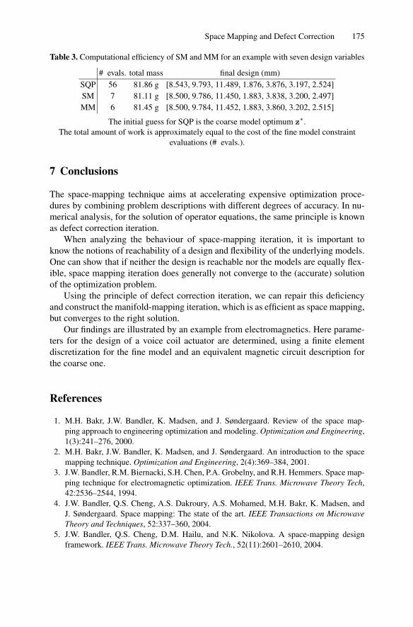
In the last example we show the potential of MM and SM in the problem with allseven design variables and non-linear equality and inequality constraints. This designproblem was introduced in [12] and details can be found in [11]. The total mass ofthe actuator has to be minimized, while the mass of the coil is constrained to 10 g.Thus, the cost function is the total mass of the device. The force at coil positionD = 4.25 mm should be kept at 5 N and the magnetic flux density in three regionsof the core should not exceed 1 T. In the fine model the constraints are evaluated bythe same FE model as used in the two previous design problems. In the coarse modelthe constraints are based on a MEC model. Each coarse model related optimizationis solved by SQP. Either MM or SM is applied for the constraints evaluation.

Numerical results for this problem are shown in Table 3. SM and MM show asimilar behaviour: convergence is reached in seven or six fine constraint evaluationsrespectively. Having the coarse model optimum z∗ as the initial guess, SQP con-verges within 56 fine constraint evaluations. MM offers an additional advantage overSM: the computation of the SM function p(x) is a very delicate issue [4], but MMreplaces it simply by the identity.


Table 3. Computational efficiency of SM and MM for an example with seven design variables

# evals. total mass final design (mm)SQP 56 81.86 g [8.543, 9.793, 11.489, 1.876, 3.876, 3.197, 2.524]SM 7 81.11 g [8.500, 9.786, 11.450, 1.883, 3.838, 3.200, 2.497]MM 6 81.45 g [8.500, 9.784, 11.452, 1.883, 3.860, 3.202, 2.515]

The initial guess for SQP is the coarse model optimum z∗.The total amount of work is approximately equal to the cost of the fine model constraint

evaluations (# evals.).

7 Conclusions

The space-mapping technique aims at accelerating expensive optimization proce-dures by combining problem descriptions with different degrees of accuracy. In nu-merical analysis, for the solution of operator equations, the same principle is knownas defect correction iteration.

When analyzing the behaviour of space-mapping iteration, it is important toknow the notions of reachability of a design and flexibility of the underlying models.One can show that if neither the design is reachable nor the models are equally flex-ible, space mapping iteration does generally not converge to the (accurate) solutionof the optimization problem.

Using the principle of defect correction iteration, we can repair this deficiencyand construct the manifold-mapping iteration, which is as efficient as space mapping,but converges to the right solution.

Our findings are illustrated by an example from electromagnetics. Here parame-ters for the design of a voice coil actuator are determined, using a finite elementdiscretization for the fine model and an equivalent magnetic circuit description forthe coarse one.

References

1. M.H. Bakr, J.W. Bandler, K. Madsen, and J. Søndergaard. Review of the space map-ping approach to engineering optimization and modeling. Optimization and Engineering,1(3):241–276, 2000.

2. M.H. Bakr, J.W. Bandler, K. Madsen, and J. Søndergaard. An introduction to the spacemapping technique. Optimization and Engineering, 2(4):369–384, 2001.

3. J.W. Bandler, R.M. Biernacki, S.H. Chen, P.A. Grobelny, and R.H. Hemmers. Space map-ping technique for electromagnetic optimization. IEEE Trans. Microwave Theory Tech,42:2536–2544, 1994.

4. J.W. Bandler, Q.S. Cheng, A.S. Dakroury, A.S. Mohamed, M.H. Bakr, K. Madsen, andJ. Søndergaard. Space mapping: The state of the art. IEEE Transactions on MicrowaveTheory and Techniques, 52:337–360, 2004.

5. J.W. Bandler, Q.S. Cheng, D.M. Hailu, and N.K. Nikolova. A space-mapping designframework. IEEE Trans. Microwave Theory Tech., 52(11):2601–2610, 2004.


6. K. Bohmer, P. W. Hemker, and H. J. Stetter. The defect correction approach. In K. Bohmerand H. J. Stetter, editors, Defect Correction Methods: Theory and Applications, Comput-ing Suppl. 5, pages 1–32. Springer-Verlag, Berlin, Heidelberg, New York, Tokyo, 1984.

7. K. Bohmer and H.J. Stetter. Defect Correction Methods: Theory and Applications.Springer, Berlin, 1984.

8. D.K. Cheng. Field and Wave Electromagnetics. Cambridge University Press, 1989.9. D. Echeverrıa and P.W. Hemker. Space mapping and defect correction. Comp. Methods

in Appl. Math., 5(2):107–136, 2005.10. D. Echeverrıa and P.W. Hemker. On the manifold mapping optimization technique. Tech-

nical Report MAS-E0612, CWI, 2006. Submitted for publication.11. D. Echeverrıa, D. Lahaye, L. Encica, E.A. Lomonova, P.W. Hemker, and A.J.A.

Vandenput. Manifold mapping optimization applied to linear actuator design. IEEE.Trans. on Magn., 42(4):1183–1186, 2006. (Also: Technical Report MAS-E0612, CWI).

12. L. Encica, D. Echeverrıa, E. A. Lomonova, A. J. A. Vandenput, P. W. Hemker, andD. Lahaye. Efficient optimal design of electromagnetic actuators using space-mapping.Struct. Multidisc. Optim., 2007. DOI 10.1007/s00158-006-0054-6. To appear. (Also in:J. Herkovits, Mazorche S, and A. Canelas, editors, Sixth World Congress on Structuraland Multidisciplinary Optimization (WCSMO6), Brazil, 2005. paper 5631).

13. L. Encica, J. Makarovic, E.A. Lomonova, and A.J.A. Vandenput. Space mappingoptimization of a cylindrical voice coil actuator. IEEE IEMDC-2005, 2005. Conferenceproceedings.

Documents

Space Mapping and Defect Correction - Stanford Universitypangea.stanford.edu/~echeverr/sfcpapers/chapter00.pdf · Space Mapping and Defect Correction ... (the ‘Aggressive Space