SOME STATISTICAL CONCEPTSChapter 3

Distributions of Data Probability Distribution

– Expected Rate of Return– Variance of Returns– Standard Deviation– Covariance– Correlation Coefficient

– Coefficient of Determination Historical Distributions

– Various Statistics

Relationship Between a Stock and the Market Portfolio– The Characteristic Line– Residual Variance

DISTRIBUTIONS OF DATA When evaluating security and portfolio returns, the

analyst may be confronted with:– 1. possible returns in some future time period

(probability distributions of possible future returns), or

– 2. past returns over some historical time period (sample distribution of past returns).

The same statistics may be used to describe both types of distributions (probability and sample). For each type of distribution, however, the procedures for calculating the various statistics vary somewhat.

In the following examples, statistics are discussed first with respect to probability distributions, and then with respect to sample distributions of historical returns.

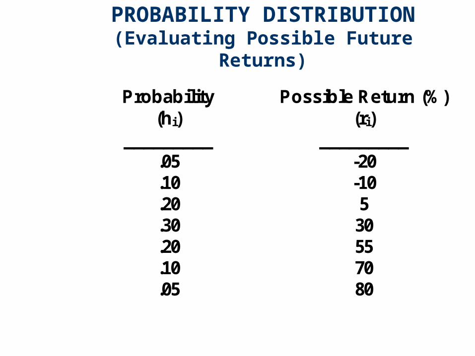
PROBABILITY DISTRIBUTION(Evaluating Possible Future Returns)

Probability (hi)

_________

Possible Return (%) (ri)

_________ .05 .10 .20 .30 .20 .10 .05

-20 -10 5

30 55 70 80

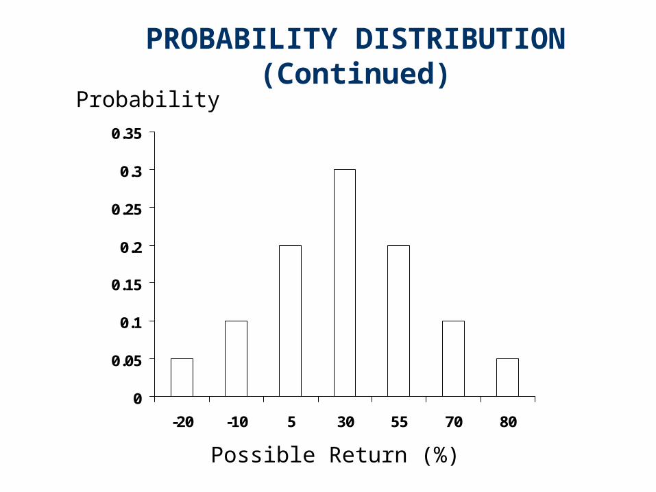
PROBABILITY DISTRIBUTION(Continued)

0

0.05

0.1

0.15

0.2

0.25

0.3

0.35

-20 -10 5 30 55 70 80

Probability

Possible Return (%)

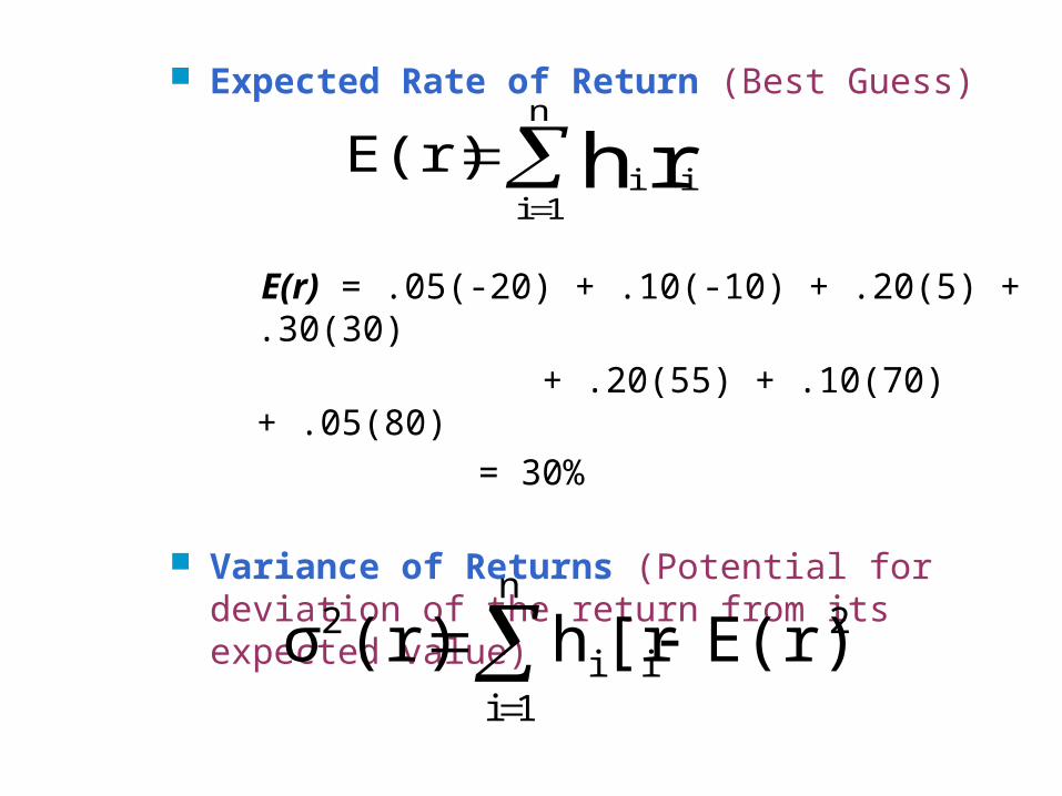
Expected Rate of Return (Best Guess)

E(r) = .05(-20) + .10(-10) + .20(5) + .30(30)

+ .20(55) + .10(70) + .05(80)

= 30%

Variance of Returns (Potential for deviation of the return from its expected value)

rh i

n

1ii

E(r)

2i

n

1ii

2 E(r)][rh(r)σ

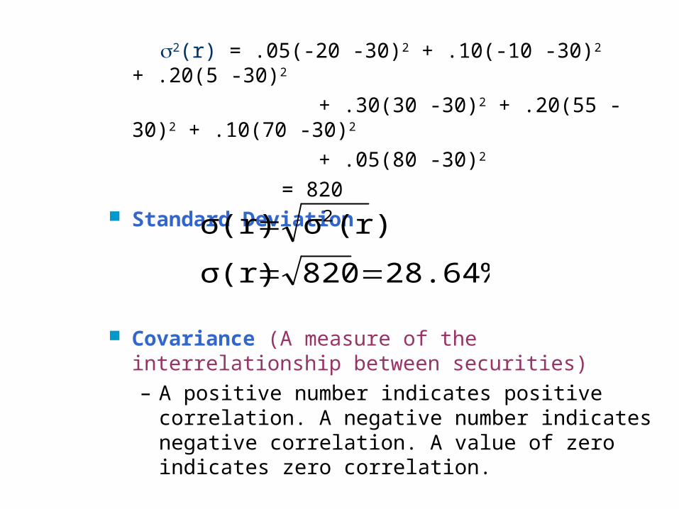
2(r) = .05(-20 -30)2 + .10(-10 -30)2 + .20(5 -30)2

+ .30(30 -30)2 + .20(55 -30)2 + .10(70 -30)2

+ .05(80 -30)2

= 820 Standard Deviation

Covariance (A measure of the interrelationship between securities)– A positive number indicates positive correlation.

A negative number indicates negative correlation. A value of zero indicates zero correlation.

28.64%820σ(r)

(r)σσ(r) 2

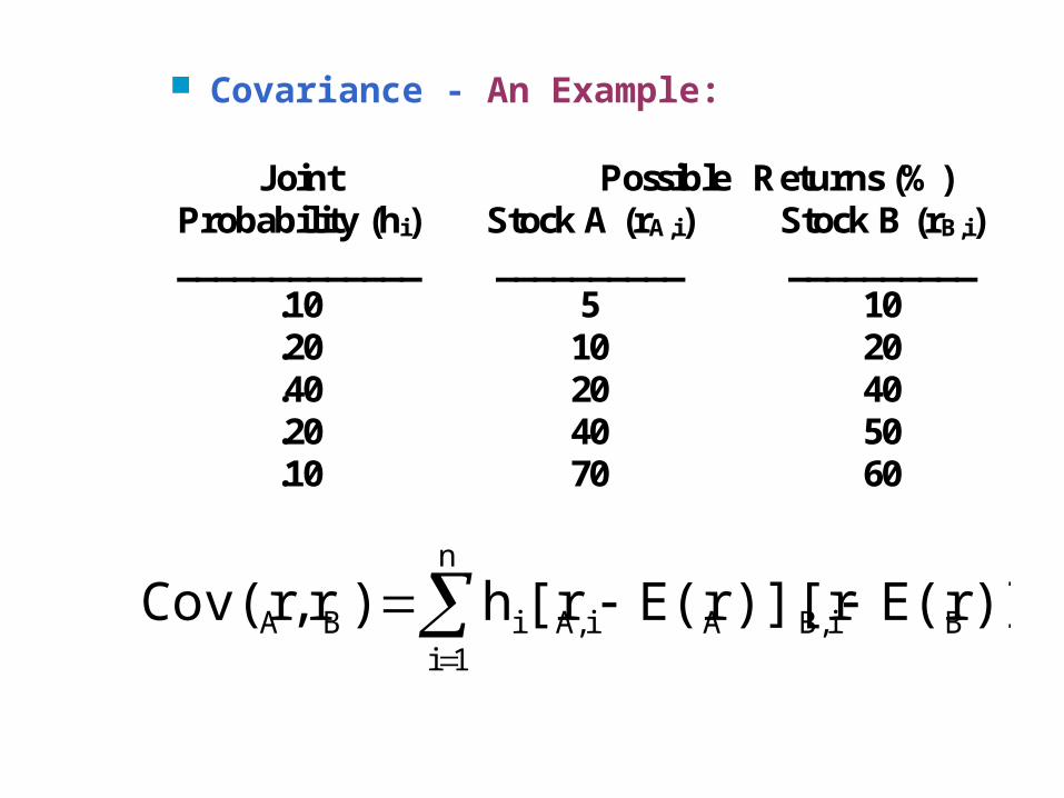
Covariance - An Example:

Joint Probability (hi) _____________

.10

.20

.40

.20

.10

Possible Stock A (rA,i) __________

5 10 20 40 70

Returns (%) Stock B (rB,i) __________

10 20 40 50 60

)]E(r)][rE(r[rh)r,Cov(r BiB,AiA,

n

1iiBA

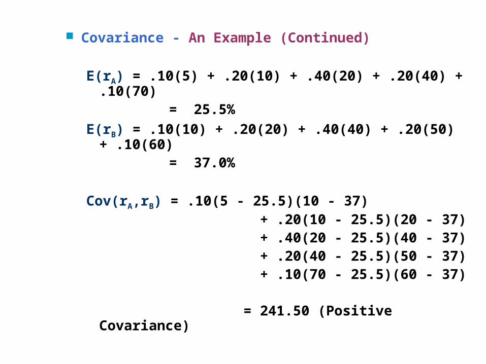
Covariance - An Example (Continued)

E(rA) = .10(5) + .20(10) + .40(20) + .20(40) + .10(70) = 25.5%

E(rB) = .10(10) + .20(20) + .40(40) + .20(50) + .10(60) = 37.0%

Cov(rA,rB) = .10(5 - 25.5)(10 - 37) + .20(10 - 25.5)(20 - 37) + .40(20 - 25.5)(40 - 37) + .20(40 - 25.5)(50 - 37) + .10(70 - 25.5)(60 - 37)

= 241.50 (Positive Covariance)

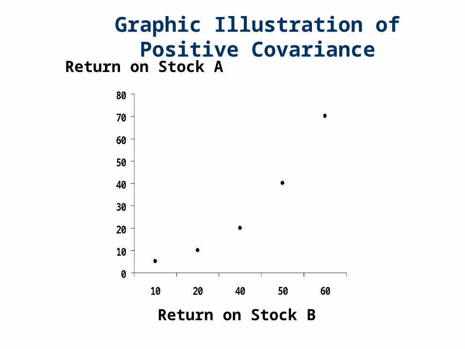
Graphic Illustration of Positive CovarianceReturn on Stock A

Return on Stock B

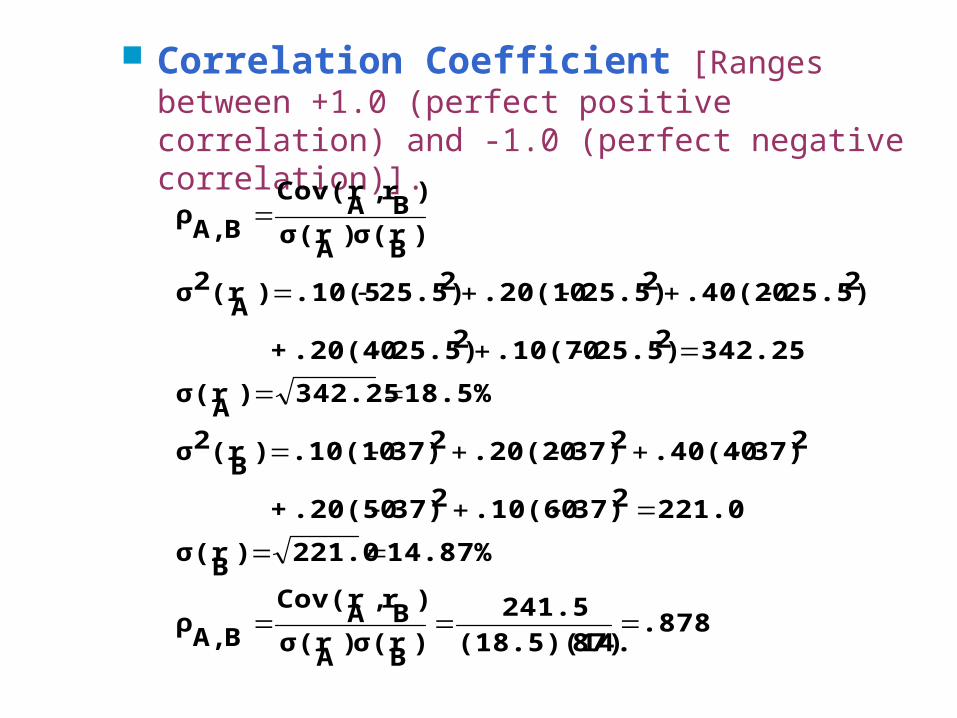
Correlation Coefficient [Ranges between +1.0 (perfect positive correlation) and -1.0 (perfect negative correlation)].

.87887)(18.5)(14.

241.5

)B

σ(r)A

σ(r

)B

r,A

Cov(r

BA,ρ

14.87%221.0)B

σ(r

221.0237).10(60237).20(50 +

237).40(40237).20(20237).10(10)B

(r2σ

18.5%342.25)A

σ(r

342.25225.5).10(70225.5).20(40 +

225.5).40(20225.5).20(10225.5).10(5)A

(r2σ

)B

σ(r)A

σ(r

)B

r,A

Cov(r

BA,ρ

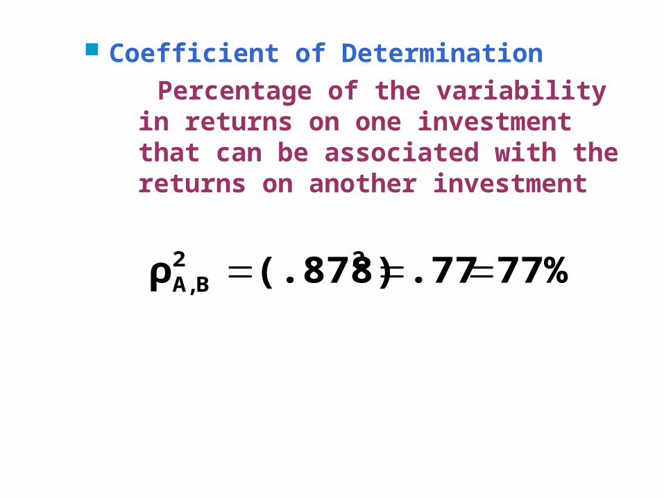
Coefficient of Determination

Percentage of the variability in returns on one investment that can be associated with the returns on another investment

77%.77(.878)ρ 22BA,

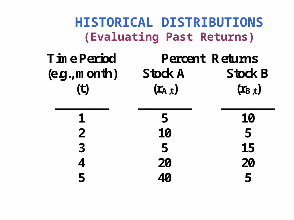
HISTORICAL DISTRIBUTIONS(Evaluating Past Returns)

Time Period (e.g., month)

(t) ________

1 2 3 4 5

Percent Stock A

(rA,t) ________

5 10 5

20 40

Returns Stock B

(rB,t) ________

10 5

15 20 5

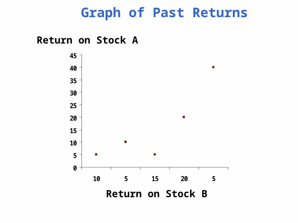
Graph of Past Returns

0

5

10

15

20

25

30

35

40

45

10 5 15 20 5

Return on Stock A

Return on Stock B

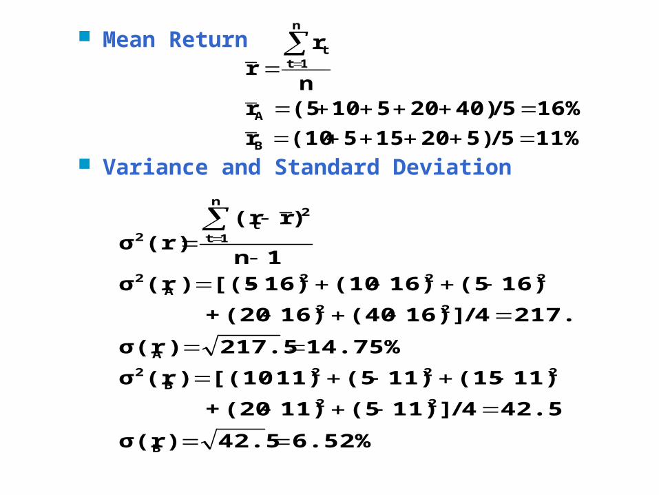
Mean Return

Variance and Standard Deviation11%5/5)20155(10r

16%5/40)20510(5rn

rr

B

A

n

1tt

6.52%42.5)σ(r

42.54/]11)(511)(20+

11)(1511)(511)[(10)(rσ

14.75%217.5)σ(r

217.54/]16)(4016)(20+

16)(516)(1016)[(5)(rσ

1n

)r(r(r)σ

B

22

222B

2

A

22

222A

2

n

1t

2t

2

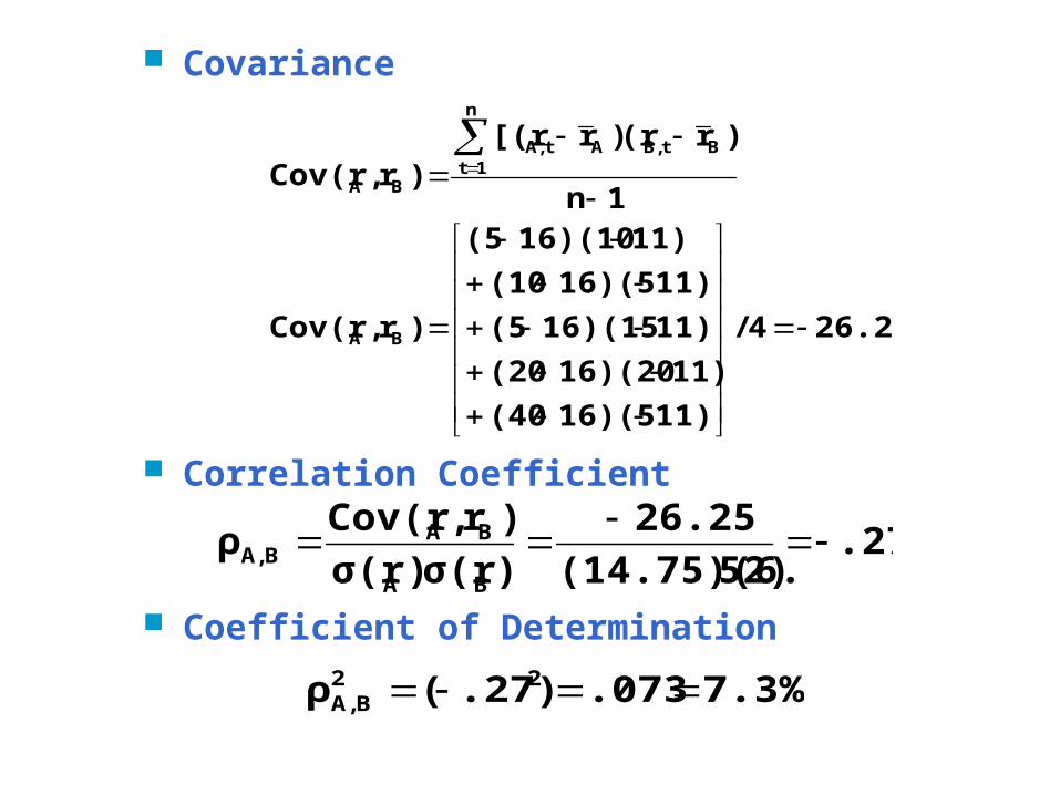
Covariance

Correlation Coefficient

Coefficient of Determination

26.254/

11)16)(5(40

11)16)(20(20

11)16)(15(5

11)16)(5(10

11)16)(10(5

)r,Cov(r

1n

)r(r)r[(r)r,Cov(r

BA

BtB,

n

1tAtA,

BA

.2752)(14.75)(6.

26.25

)σ(r)σ(r

)r,Cov(rρ

BA

BABA,

7.3%.073.27)(ρ 22BA,

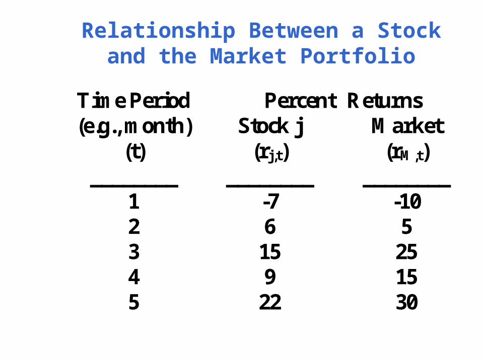
Relationship Between a Stock and the Market Portfolio

Time Period (e.g., month)

(t) ________

1 2 3 4 5

Percent Stock j

(rj,t) ________

-7 6

15 9

22

Returns Market

(rM,t) ________

-10 5

25 15 30

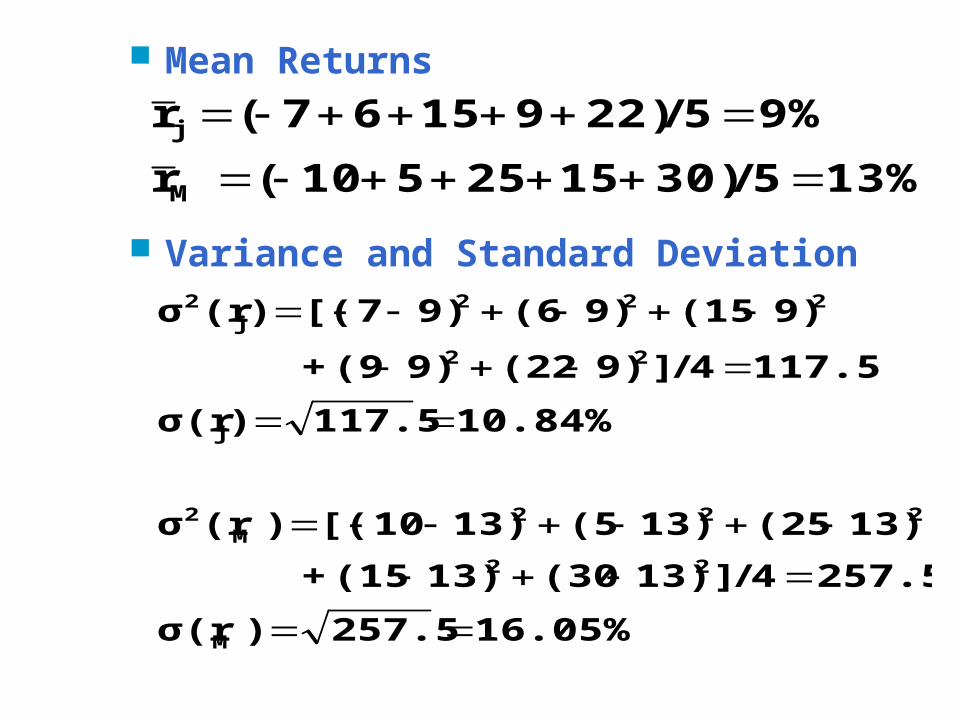
Mean Returns

Variance and Standard Deviation

13%5/30)1525510(r

9%5/22)91567(r

M

j

16.05%257.5)σ(r

257.54/]13)(3013)(15+

13)(2513)(513)10[()(rσ

10.84%117.5)σ(r

117.54/]9)(229)(9+

9)(159)(69)7[()(rσ

M

22

222M

2

j

22

222j

2

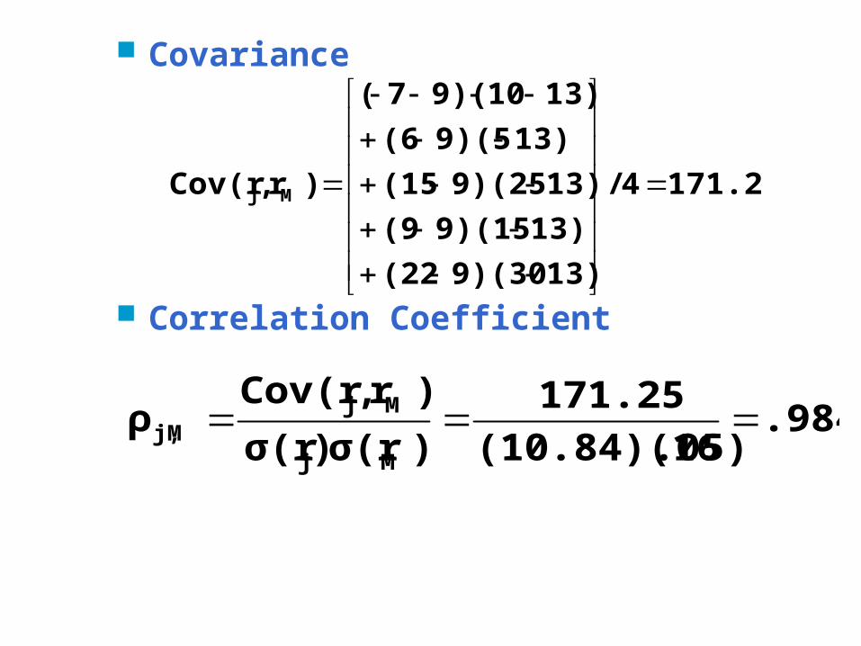
Covariance

Correlation Coefficient

171.254/

13)9)(30(22

13)9)(15(9

13)9)(25(15

13)9)(5(6

13)109)(7(

)r,Cov(r Mj

.984.05)(10.84)(16

171.25

)σ(r)σ(r

)r,Cov(rρ

Mj

MjMj,

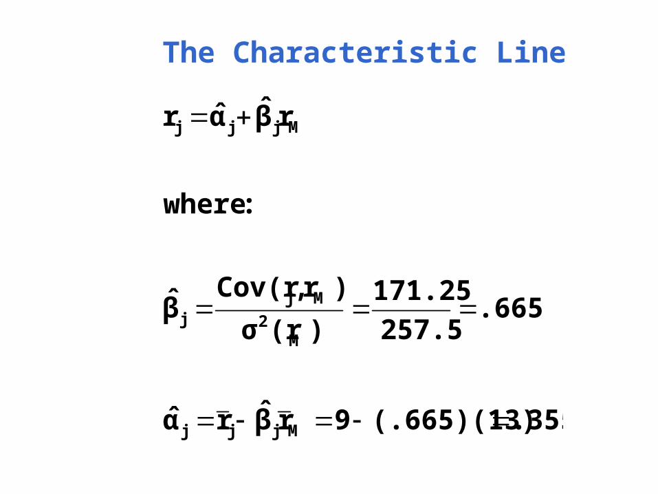
The Characteristic Line

.355 (.665)(13)9rβ̂rα̂

.665 257.5

171.25

)(rσ

)r,Cov(rβ̂

:where

rβ̂α̂r

Mjjj

M2

Mjj

Mjjj

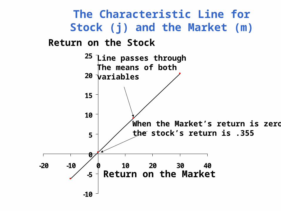
The Characteristic Line forStock (j) and the Market (m)

-10

-5

0

5

10

15

20

25

-20 -10 0 10 20 30 40

Return on the Stock

Return on the Market

Line passes throughThe means of bothvariables

When the Market’s return is zero,the stock’s return is .355

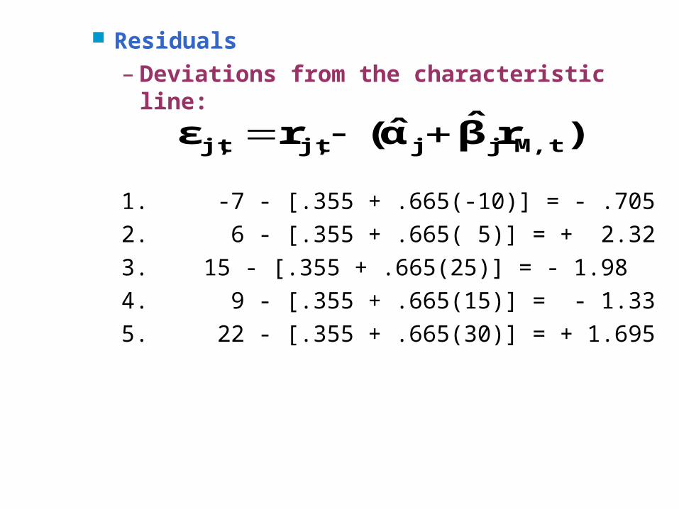
Residuals– Deviations from the characteristic line:

1. -7 - [.355 + .665(-10)] = - .705

2. 6 - [.355 + .665( 5)] = + 2.32

3. 15 - [.355 + .665(25)] = - 1.98

4. 9 - [.355 + .665(15)] = - 1.33

5. 22 - [.355 + .665(30)] = + 1.695

)rβ̂α̂(rε tM,jjtj,tj,

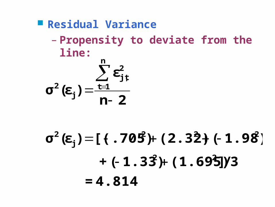
Residual Variance– Propensity to deviate from the line:

4.814 =

3/](1.695)1.33)( +

1.98)((2.32).705)[()(εσ

2n

ε)(εσ

22

222j

2

n

1t

2tj,

j2