Modelling heterogeneous variance-covariance components

in two-level multilevel models with application to school effects

educational research

Research Methods Festival Oxford

9th July 2014

George Leckie Centre for Multilevel Modelling Graduate School of Education

University of Bristol

1. INTRODUCTION

The standard two-level random-slope multilevel model

• The standard two-level (e.g. students within schools or repeated measures within subjects) random-slope multilevel model can be written as

𝑌𝑖𝑗 = 𝛽0 + 𝛽1𝑋𝑖𝑗

fixed part

+ 𝑢0𝑗 + 𝑢1𝑗𝑋𝑖𝑗 + 𝑒𝑖𝑗

random part

where

𝑢0𝑗

𝑢1𝑗~N

00

,𝜎𝑢0

2

𝜎𝑢0𝑢1 𝜎𝑢12

𝑒𝑖𝑗~N(0, 𝜎𝑒2)

• Every school is modelled as having its own regression line with its own intercept, 𝛽0 + 𝑢0𝑗 , and its own slope, 𝛽1 + 𝑢1𝑗 , but all school are constrained

to have a common residual error variance, 𝜎𝑒2

• However, it will often be substantively interesting to model this residual error variance as heterogeneous across students and schools, 𝜎𝑒𝑖𝑗

2

What we do

• We extend the standard random-slope model by modelling the level-1 variance as a log-linear function of the covariates and further random effects

Mean function: 𝑌𝑖𝑗 = 𝛽0 + 𝛽1𝑋𝑖𝑗

fixed part

+ 𝑢0𝑗 + 𝑢1𝑗𝑋𝑖𝑗 + 𝑒𝑖𝑗

random part

Level-1 variance function: log 𝜎𝑒𝑖𝑗2 = 𝛼0 + 𝛼1𝑋𝑖𝑗

fixed part

+ 𝑣0𝑗 + 𝑣1𝑗𝑋𝑖𝑗

random part

where

𝑢0𝑗

𝑢1𝑗

𝑣0𝑗

𝑣1𝑗

~N

0000

,

𝜎𝑢02

𝜎𝑢01 𝜎𝑢12

𝜎𝑢0𝑣0 𝜎𝑢1𝑣0 𝜎𝑣02

𝜎𝑢0𝑣1 𝜎𝑢1𝑣1 𝜎𝑣01 𝜎𝑣12

, 𝑒𝑖𝑗~N(0, 𝜎𝑒𝑖𝑗2 )

• We won’t discus modelling the different variances and covariances of the level-2 covariance matrix as a function of the covariates, but this is possible

2. SOFTWARE

Likelihood-based methods

• Not possible to fit these models using routine commands in general-purpose packages such as R, SAS, SPSS and Stata, nor is it possible to fit these models in dedicated multilevel modelling packages such as MLwiN, HLM, and SuperMix

• ASReml and GenStat: Assume independent random effects

• SAS PROC NLMIXED: Two-level models only; slow; sensitive to starting values

• MIXREGLS: Developed by Don Hedeker; Two-level random-intercept models only; computationally faster and more stable than SAS; fiddly to use

– We have written runmixregls, a command to call MIXREGLS from within

Stata – http://www.bristol.ac.uk/cmm/software/runmixregls/

MCMC methods

• WinBUGS: Highly flexible; fiddly to use; computationally fairly slow

• Stat-JR: Easy to use, computationally faster than WinBUGS, developed by the MLwiN team!

– We have developed a 2LevelRSCVGL template to fit this calls of model

– Need a better name!

– http://www.bristol.ac.uk/cmm/software/statjr/

3. ILLUSTRATIVE APPLICATION

Studies of school effects

• Most studies of school effects focus on estimating mean differences in student achievement

– Which schools score highest, having adjusted for intake differences?

– What school polices and practices make some schools more effective than others?

• Rarely is anything said about whether there might be variance differences in student achievement

• However, just as schools influence the mean achievement of their students, they are likely to influence the dispersion in their students’ achievements

– Which schools widen initial inequalities and which schools narrow them?

– What school polices and practices drive these differences?

Inner-London schools’ exam scores dataset

• MLwiN ‘tutorial’ dataset

• 4,059 students (level-1) nested within 65 schools (level-2)

• 2 to 198 students per school (mean = 62 students)

• Response is a standardised age 16 exam score

• Main covariates are

– A standardised age 11 exam score

– Student gender

Observed school means and within-school variances

• There is substantial variability in both school means and within-school variances

• There is a moderate positive association between the two (𝑟 = 0.29)

Specify a log-linear level-1 variance function

• First we specify a log-linear level-1 variance function for the within-school variance and we include a new set of school random effects

Mean function 𝐒𝐂𝐎𝐑𝐄𝟏𝟔𝑖𝑗 = 𝛽0 + 𝑢𝑗 + 𝑒𝑖𝑗

𝑢𝑗~N 0, 𝜎𝑢2

𝑒𝑖𝑗~N(0, 𝜎𝑒𝑗2 )

log(𝜎𝑒𝑗2 ) = 𝛼0 + 𝑣𝑗

𝑣𝑗~N 0, 𝜎𝑣2

where 𝑢𝑗 and 𝑣𝑗 are allowed to covary with covariance 𝜎𝑢𝑣 (correlation 𝜌𝑢𝑣)

• Every school has its own mean 𝛽0𝑗 = 𝛽0 + 𝑢𝑗 and variance 𝜎𝑒𝑗2 = exp (𝛼0 + 𝑣𝑗)

Level-1 variance function

Random within-school variances

• Model 1 is simply a reparameterised variance-components model where

log 𝜎𝑒2 = 𝛼0

• Model 2 includes the new school random effects

log(𝜎𝑒𝑗2 ) = 𝛼0 + 𝑣𝑗 , 𝑣𝑗~N 0, 𝜎𝑣

2

• Model 2 is preferred to Model 1 as shown by drop in DIC of 127 points

• Note that the estimated intercept has decreased from -0.17 to -0.22. Why?

Model 1 Model 2

Parameter Mean SD Mean SD

Mean function 𝛽0 Intercept -0.02 0.06 -0.02 0.05

𝜎𝑢2 Intercept variance 0.18 0.04 0.19 0.04

Level-1 variance function

𝛼0 Intercept -0.17 0.02 -0.22 0.05

𝜎𝑣2 Intercept variance − − 0.11 0.03

Cross-function 𝜌𝑢𝑣 Correlation − − 0.36 0.14

DIC 10910 10783

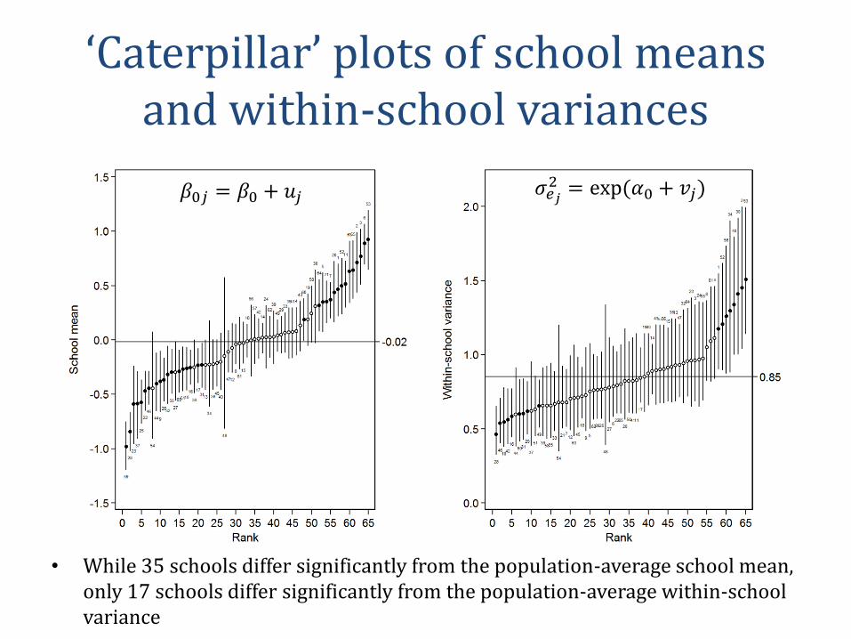
‘Caterpillar’ plots of school means and within-school variances

• While 35 schools differ significantly from the population-average school mean, only 17 schools differ significantly from the population-average within-school variance

𝛽0𝑗 = 𝛽0 + 𝑢𝑗 𝜎𝑒𝑗2 = exp (𝛼0 + 𝑣𝑗)

Caterpillar plot of intraclass correlation coefficients

• The expected correlation between two students from the same school ranges from 0.11 to 0.29

• Few schools differ significantly from the population-average correlation of 0.18

corr 𝑦𝑖𝑗 , 𝑦𝑖′𝑗 =𝜎𝑢

2

𝜎𝑢2 + exp (𝛼0 + 𝑣𝑗)

Add covariates to the mean function

• 𝛽1 = 0.55 and so age 11 scores are strongly predictive of age 16 scores

• 𝛽2 = 0.17 and so girls make more progress than similar initial achieving boys

• Between-school variance 𝜎𝑢2 reduces by 47%

• Population-average of the within-school variances E(𝜎𝑒𝑗2 ) reduces by 33%

• Population-variance of the within-school variances Var(𝜎𝑒𝑗2 ) reduces by 78%

Model 2 Model 3

Parameter Mean SD Mean SD

Mean function

𝛽0 Intercept -0.02 0.05 -0.09 0.05

𝛽1 Age 11 scores − − 0.55 0.01

𝛽2 Girl − − 0.17 0.03

𝜎𝑢2 Intercept variance 0.19 0.04 0.10 0.02

Level-1 variance function

𝛼0 Intercept -0.22 0.05 -0.60 0.04

𝜎𝑣2 Intercept variance 0.11 0.03 0.06 0.02

Cross-function 𝜌𝑢𝑣 Correlation 0.36 0.14 0.03 0.01

DIC 10783 9194

Add a random slope to the mean function

• Are schools differentially effective for different types of students? – Are the schools that are best for high initial achievers different from the

schools that are best for low initial achievers?

– Does the gender gap vary across schools? Are there some schools where boys actually outperform girls?

• Model 4 allows the age 11 slope coefficient to vary across schools 𝐒𝐂𝐎𝐑𝐄𝟏𝟔𝑖𝑗 = 𝛽0 + 𝛽1𝐒𝐂𝐎𝐑𝐄𝟏𝟏𝑖𝑗 + 𝛽2𝐆𝐈𝐑𝐋𝑖𝑗 + 𝑢0𝑗 + 𝑢1𝑗𝐒𝐂𝐎𝐑𝐄𝟏𝟏𝑖𝑗 + 𝑒𝑖𝑗

log(𝜎𝑒𝑗2 ) = 𝛼0 + 𝑣𝑗

𝑢0𝑗

𝑢1𝑗

𝑣𝑗

~N000

,

𝜎𝑢02

𝜎𝑢01 𝜎𝑢12

𝜎𝑢0𝑣 𝜎𝑢1𝑣 𝜎𝑣2

𝑒𝑖𝑗~N(0, 𝜎𝑒𝑗2 )

Predicted mean function school lines

• Age 11 scores are more predictive of age 16 scores in some schools than in others

• Schools with steeper slopes widen initial achievement differences

• School choice matters more for high initial achievers?

Add covariates to the level-1 variance function

• The mean function parameters hardly change and are omitted from the table

• 𝛼1 = −0.07 and so, within schools, low initial achievers tend to score more variably than high initial achievers

• 𝛼2 = −0.10 and so, within schools, girls tend to score less variably than boys

Model 4 Model 5

Parameter Mean SD Mean SD

Mean function … … … … … …

Level-1 variance function

𝛼0 Intercept -0.63 0.04 -0.57 0.05

𝛼1 Age 11 scores − − -0.07 0.02

𝛼2 Girl − − -0.10 0.05

𝜎𝑣2 Intercept variance 0.06 0.02 0.06 0.02

Cross-function 𝜌𝑢0𝑣 Intercept-intercept correlation 0.40 0.17 0.45 0.15

𝜌𝑢1𝑣 Slope-intercept correlation 0.76 0.14 0.77 0.13

DIC 9133 9121

Add a random slope to the level-1 variance function

• Do schools have differentially dispersed outcomes for different types of students? – Are the schools that are least dispersed for high initial achievers different

from the schools that are least dispersed for low initial achievers?

– Does the gender dispersion gap vary across schools?

• Model 6 adds a random slope to the level-1 variance function 𝐒𝐂𝐎𝐑𝐄𝟏𝟔𝑖𝑗 = 𝛽0 + 𝛽1𝐒𝐂𝐎𝐑𝐄𝟏𝟏𝑖𝑗 + 𝛽2𝐆𝐈𝐑𝐋𝑖𝑗 + 𝑢0𝑗 + 𝑢1𝑗𝐒𝐂𝐎𝐑𝐄𝟏𝟏𝑖𝑗 + 𝑒𝑖𝑗

log(𝜎𝑒𝑖𝑗2 ) = 𝛼0 + 𝛼1𝐒𝐂𝐎𝐑𝐄𝟏𝟏𝑖𝑗 + 𝛼2𝐆𝐈𝐑𝐋𝑖𝑗 + 𝑣0𝑗 + 𝑣1𝑗𝐒𝐂𝐎𝐑𝐄𝟏𝟏𝑖𝑗

𝑢0𝑗

𝑢1𝑗

𝑣0𝑗

𝑣1𝑗

~N

0000

,

𝜎𝑢02

𝜎𝑢01 𝜎𝑢12

𝜎𝑢0𝑣0 𝜎𝑢1𝑣0 𝜎𝑣02

𝜎𝑢0𝑣1 𝜎𝑢1𝑣1 𝜎𝑣01 𝜎𝑣12

𝑒𝑖𝑗~N(0, 𝜎𝑒𝑖𝑗2 )

Predicted level-1 variance function school ‘lines’

• Three schools actually go against the overall trend and should be examined further

• What is it about these three schools which leads their highest initial achieving students to perform more erratically than their lowest initial achieving students?

Explaining the differences between schools

• So far we have quantified differences in effectiveness and dispersion between schools and how the magnitude of these differences vary as function of initial achievement

• The obvious next step is to seek to explain these differences in terms of school-level predictors 𝑊𝑗

– Entering 𝑊𝑗 as a main effect into the mean function will explain away 𝜎𝑢02

– Entering 𝑊𝑗 as a cross-level interaction with 𝑋𝑖𝑗 into the mean function

will explain away 𝜎𝑢12

– Entering 𝑊𝑗 as a main effect into the level-1 variance function will explain

away 𝜎𝑣02

– Entering 𝑊𝑗 as a cross-level interaction with 𝑋𝑖𝑗 into the level-1 variance

function will explain away 𝜎𝑣12

4. SIMULATION STUDY

Can we ignore the random effects?

• Many packages allow you to fit limited level-1 variance functions with no random effects

– R, SAS, SPSS, Stata

– HLM, MLwiN

• However, we have carried out simulations which show that ignoring level-2 variability in the level-1 variances leads the level-1 variance function regression coefficients to be estimated with spurious precision

– This problem is particularly acute for the coefficients of level-2 covariates

– We run the risk of making Type I errors of inference about predictors of level-1 variance

– This problem is analogous to ignoring clustering in linear regression

5. CONCLUSION

Conclusion

• We have extended the standard two-level random-slope model to model the residual error variance as a function of the covariates and additional random effects

• We are implementing this in runmixregls and the new Stat-JR software

– http://www.bristol.ac.uk/cmm/software/runmixregls/

– http://www.bristol.ac.uk/cmm/software/statjr

• The principle of modelling within-group variances as randomly varying across groups applies to multilevel models more generally, including those with additional levels, crossed random effects and discrete responses

• The discussed methods are relevant to any study where there is interest on estimating dispersion differences on outcome variables across groups

References to our work

• Goldstein, H., Leckie, G., Charlton, C., and Browne, W. Multilevel models with random effects for level 1 variance functions, with application to child growth data. Submitted.

• Leckie, G. (2013). Modeling the residual error variance in Two-Level Random-Coefficient Multilevel Models. Bulletin of the International Statistical Institute, 68, 1-6.

• Leckie, G. (2014). runmixregls - A Program to Run the MIXREGLS Mixed-effects Location Scale Software from within Stata. Journal of Statistical Software, Code Snippet, 1-41. Forthcoming.

• Leckie, G., French, R., Charlton, C., and Browne, W. (2015). Modeling Heterogeneous Variance-Covariance Components in Two-Level Models. Journal of Educational and Behavioral Statistics. Forthcoming.

References to other work

• Hedeker, D., Mermelstein, R. J., & Demirtas, H. (2008). An Application of a Mixed-Effects Location Scale Model for Analysis of Ecological Momentary Assessment (EMA) Data. Biometrics, 64, 627-634.

• Lee, Y., & Nelder, J. A. (2006). Double hierarchical generalized linear models (with discussion). Applied Statistics, 55, 139–185.

• Rast, P., Hofer, S. M., & Sparks, C. (2012). Modeling individual differences in within-person variation of negative and positive affect in a mixed effects location scale model using BUGS/JAGS. Multivariate Behavioral Research, 47, 177-200.

What about modelling the level-2 variance-covariance matrix?

• It is relatively easy to model a 2 × 2 variance-covariance matrix as a function of the covariates

𝑢𝑗

𝑣𝑗~N

00

,𝜎𝑢𝑗

2

𝜎𝑢𝑣𝑗𝜎𝑣𝑗

2

log 𝜎𝑢𝑗2 = 𝜅0 + 𝜅1𝑊𝑗

log 𝜎𝑣𝑗2 = 𝛾0 + 𝛾1𝑊𝑗

tanh−1 𝜌𝑢𝑣𝑗 = 𝛿0 + 𝛿1𝑊𝑗

• However, simply specifying appropriate link functions will no longer ensure positive definiteness in 3 × 3 and larger variance-covariance matrices

– In MCMC sampler, reject any proposed parameter values which give rise to variance-covariance matrices which are not positive definite