Some aspects of the HARMONIE limited-area model · ECMWF Seminar, September 2013 1 Some aspects of the HARMONIE limited-area model Mariano Hortal Project Leader on Dynamics. HIRLAM

ECMWF Seminar, September 2013 1

Some aspects of the HARMONIE

limited-area model

Mariano Hortal Project Leader on Dynamics. HIRLAM


Outlook

• Vertical discretization using finite elements • Spectral discretization in the horizontal

– Spectral basis – Biperiodization – Relaxation to the nesting model – Application of relaxation and biperiodization in

spectral space • Elimination of the extension zone from the grid-

point representation and increase of the width of the extension zone


Vertical discretization using finite elements (F.E.)

• In the hydrostatic version the only vertical operator is the integral

• In the non-hydrostatic version both the integral and the derivative are needed – This introduces some constraints when arriving at a

Helmholtz equation – These constraints are not fulfilled by the F.E.

operators


Construction of a vertical operator

ηddfF =

∑=

M

i

ii EFF

1)(~)( ηη

∑=

N

i

iieff

1)(~)( ηη

Approximate functions as linear combinations of basis functions

∑∑==

≈N

j

jj

M

i

ii e

ddfEF

11)()( η

ηη

Derivative operator


Galerkin procedure

( ) ( ) ( ) ( )KkdTeddfdTEF

N

jk

jj

M

ik

ii −∈∀=∑ ∫∑ ∫

==

1)(1

1

01

1

0ηηη

ηηηη

Approximation error: orthogonal to space spanned by test functions T

Aik

(mass matrix) Bj

k (operator matrix)

BA fFBfAFN

j

jkj

M

i

iki

~~11

=⇒=∑∑==

K equations M unknowns

Scalarly multiply by a set of test functions


If we are given the values at a set of values of

Galerkin procedure (cont)

f~

( )ηf

( )jf η

is the set of coefficients for the representation of function

η

(full level values)

( ) ( )

( ) 1

1~

~

−

=

=

≡=∑P

P

j

M

ij

iij

ff

feff

η

ηη1−P is the projection

matrix to the space spanned by the basis functions e


Galerkin procedure (cont)

F~

( ) ( ) SFEFFN

jl

jjl

~1

≡=∑=

ηη

S

From the vector of values We can get the values of the function at full levels

Where Is the inverse projection matrix from the space spanned by the basis E

( ) ( ) ( )MSBAPSBAS jjj fffFF ηηη ≡=== −−− 111~~


Vertical operators (cont)

• Matrix M applied to the set of full-level values of field f gives the set of full-level values of its derivative

• Similarly we can compute the matrix for the integral operator: N

• The order of accuracy of both M and N, using cubic basis functions can be shown to be 8

• M and N are NOT the inverse of each other


Equations

( ) ( )

pRTm

gwdtd

TCQppD

CC

dtdp

CQ

dtdp

pCRT

dtdT

mmtm

pm

gdtdw

pm

pp

RTdtd

vv

p

pp

−=∂∂

=

=+

=−

=∂∂

+∇+∂∂

Ω=

∂∂

−+

=∇∂∂

+∇+

πφ

φ

ηη

γη

γ

ςφη

η

ηη

3

1

0

11

1

V

V


Pressure departure and Vertical divergence

ηρ

ππ

∂∂

−=

−=

wm

gd

pP

( ) ( ) ( )

∂∂

−−−=

++

++−=

−+=

η

πππ

π

wdtd

mRTpg

dtdm

mdtdT

Tdtdp

pdtd

TCQPD

CC

Pdtd

dtdp

pP

dtdP

vv

p

1d1d1dd

11111 3

The corresponding equations are


Helmholtz equation

( ) ( ) ...d1 *22*

2*

2*4

2*

*22

*2*

2 shrTmrcNt

rHmct =

∇∆−

+∇∆−

L

Eliminating from the discretized set of equations (with some constraints to be fulfilled by the operators) all the variables except the vertical divergence, we obtain a Helmholtz equation:

Which can be solved very easily in spectral space In a projection on vertical eigenvectors


Choices to apply VFE in the NH version

• Choose a set of equations using only one vertical operator – Change the set of forecast fields – Change the vertical coordinate to one based on

height instead of mass • Solve a set of two coupled equations instead of

a single Helmholtz equation


Change of the vertical coordinate to a height-based hybrid one

• Use of a time-independent coordinate eliminates the X-term.

• Only derivatives are used in the vertical (no integrals) which simplifies the constraints to arrive at a single Helmholtz equation

• The coordinate is still a hybrid coordinate. The data flow is maintained.


Change the vertical coordinate

• Juan Simarro has tested this option. • Any vertical discretization, either finite

differences or finite elements of accuracy order greater than 4 becomes unstable

Note: In general higher accuracy leads to lower stability


Solve a coupled system of equations (Jozef Vivoda & Petra Smolikova)

• In order to arrive at a single Helmholtz equation, the following constraint (C1) has to be fulfilled

0*****1 =+−−≡ NGSSGA

Where

( ) ∫≡ l dmSl

l

ηηψ

πψ

0

**

* 1

( ) ∫≡1

*

**

ηηψ

πψ dmG l

( ) ( ) 1**

+≡ Ll SN ψψ

As this constraint is not fulfilled with the finite-elements integral operator, we cannot arrive at a single Helmholtz equation


Solve a coupled system of equations (cont)

Instead, we arrive at a coupled system involving both The horizontal and the vertical divergences

where


Solve a coupled system of equations (cont)

• The system of equations is twice as large as in the hydrostatic case

• An iterative procedure has been adopted for solving the system

• This method is being implemented in both HARMONIE and IFS


Spectral horizontal discretization

• Spherical harmonics are not an appropriate basis for a limited-area domain

• The model equations are solved on a plane projection with Cartesian x-y coordinates

• Double Fourier functions are used as the basis for spectral discretization

• Fields should be periodic in both x and y • An extension zone is used to biperiodize the

fields


Biperiodization of fields

Lx

Ly

∑∑−= −=

≈I

Ii

J

Jj

LjlyLikxlk

yx eefyxF //),(

Periodic in x (period Lx) and in y (period Ly)


Boundary conditions

Central Zone (C) Boundary

Zone (I)

Extension Zone (E)


Boundary conditions Gabor Radnoti 1995

( )ttttttt ttI Ψ−Ψ∆+Ψ=Ψ∆− ∆−∆+∆+ 2)( (exp) LL

( ) LSlC Ψ⋅+Ψ⋅−=Ψ αα1

Ψ~

( ) ( ) ( ) LStt

ltt tItI ∆+∆+ Ψ∆−+Ψ−=Ψ∆− LL αα1

Semi-implicit solution procedure:

Coupling to a nesting model (LS)

Implementation:

α =1 at the whole of E. α =0 at the whole of C Smoothly changing at I


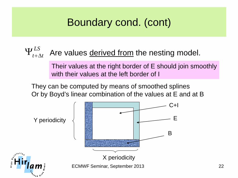
Boundary cond. (cont)

LStt ∆+Ψ Are values derived from the nesting model.

Their values at the right border of E should join smoothly with their values at the left border of I

They can be computed by means of smoothed splines Or by Boyd’s linear combination of the values at E and at B

Y periodicity

C+I

E

B

X periodicity


Increasing the width of E

• In data assimilation the influence of an observation covers an area around the observation position

• Due to the periodicity of fields, an observation close to the right border of the inner domain can affect the fields on the left border.

• That can be eliminated by increasing the width of the extension zone


Increasing the width of E (cont)

• If the points in the extension zone are present in the grid-point representation – The cost of running the model increases if we increase the width

of E – Due to the clipping of the semi-Lagrangian trajectories to the C+I

area, the interpolation points could fall outside the semi-Lagrangian buffer, producing floating-point errors or segmentation faults

• Elimination of the extension zone from the grid-point representation – Application of the boundary conditions and biperiodization in

spectral space

Documents

Some aspects of the HARMONIE limited-area model · ECMWF Seminar, September 2013 1 Some aspects of the HARMONIE limited-area model Mariano Hortal Project Leader on Dynamics. HIRLAM