Embed Size (px)
Citation preview

SOME ASPECTS OF KALMAN FILTERING
M. A. SALZMANN
August 1988
TECHNICAL REPORT NO. 140

PREFACE
In order to make our extensive series of technical reports more readily available, we have scanned the old master copies and produced electronic versions in Portable Document Format. The quality of the images varies depending on the quality of the originals. The images have not been converted to searchable text.
SOME ASPECTS OF KALMAN FILTERING
Martin A. Salzmann
Department of Geodesy and Geomatics Engineering University of New Brunswick
P.O. Box 4400 Fredericton, N .B.
Canada E3B 5A3
August 1988 Latest Reprinting February 1996

ABSTRACT
In hydrography and surveying the use of kinematic positioning techniques is
nowadays very common. An optimal estimate of position of the kinematic user is
usually obtained by means of the Kalman filter algorithm. Dynamic and measurement
models are established for a discrete time, time varying system. Some problems in
establishing such a model are addressed. Based on this model and the derived Kalman
filter several aspects of Kalman filtering that are important for kinematic positioning
applications are discussed.
Computational and numerical considerations indicate that so-called covariance
filters are to be used for kinematic positioning, and a specific covariance filter
mechanization is described in detail. For some special applications linear smoothing
techniques lead to considerably improved estimation results. Possible applications of
smoothing techniques are reviewed. To guarantee optimal estimation results the
analysis of the performance of Kalman filters is essential. Misspecifications in the
filter model can be detected and diagnosed. The performance analysis is based on the
innovation sequence.
Overall, this report presents a detailed analysis of some aspects of Kalman
filtering.
Ill
TABLE OF CONTENTS
Page
ABSTRACT............................................................................ m TABLE OF CONTENTS . . . . . . . . . . . . . . . . . . . . . . . . . . . . . . . . . . . . . . . . . . .. . . . . . . . . . . . . . . . 1v
LIST OF FIGURES ................................................................. vi ACKNOWLEDGEMENTS .............................. ....... .. ............... .. vn
1. INTRODUCTION . . . . . . . . . . .. . . . . . . . . . . . . . . . . . . . . . . . . . . . . . . . . . . . . .. . . . . . . . . . . . . . . 1
2. THE LINEAR KALMAN FILTER .. . . . .. . . . . . . .. . . . . . . . . . . . . . . . . . . . . . . . . . . 5 2.1 System Model and the Linear Kalman Filter . . . . . . . . . . . . . . . . . . . . . . . . . . . . . . . . 5 2.2 The Linear Kalman Filter: A Derivation Based on Least Squares ........ 9 2.3 Extensions of the System Model . . . . . . . . . . . . . . . . . . . . . . . . . . . . . . . . . . . . . . . . . . . . . 13
2.3.1 Alternative System Models ........................... ........... ....... 13 2.3.2 Model Nonlinearities . . . . . . . . . . . . . . . . . . . . . . . . . . . . . . . . . . . . . . . . . . . . . . . . . . . . 17 2.3.3 Filter Design Considerations . . . .. . . .. . . . . . . . .. . . .. . . .. . . . . . . . .. . . .. . . .. 19 2.3.4 Alternative Noise Models . . . . . . . . . . . . . . . . . . . . . . . . . . . . . . . . . . . . . . . . . . . . . . 21
2.4 Final Model Considerations . . . . . . . . . . . . . . . . . . . . . . . . . . . . . . . . . . . . . . . . . . . . . . . . . . . 22
3. COMPUTATIONAL CONSIDERATIONS .............................. 25 3.1 Introduction .......................................... ......................... .. 25 3.2 Basic Filter Mechanizations . . . . . . . . . . . . . . . . . . . . . . . . . . . . . . . . . . . . . . . . . . . . . . . . . . . 26 3.3 Square Root Filtering . . . . . . . . . . . . . . . . . . . . . . . . . . . . . . . . . . . . . . . . . . . . . . . . . . . . . . . . . . 30
3.3.1 Square Root Covariance Filter .................... .. ................... 31 3.3.2 Square Root Information Filter . . . . . . . . . . . . . . . . . . . . . . . . . . . . . . . . . . . . . . . . 32
3.4 U-D Covariance Factorization Filter ................. ......... ............... 33 3.4.1 U-D Filter Measurement Update ................... ....... ...... ....... 34 3.4.2 U-D Filter Time Update . . . . . . . . . . . . . . . . . . .. . . . . . . . . . . . . . . . . . . .. . . . . . . .. 36
3.5 Implementation Considerations . . . . . . . . . . . . . . . . . . . . . . . . . . . . . . . . . . . . . . . . . . . . . . . 40 3.5 .1 Computational Efficiency . . . . . . . . . . . . . . . . . . . . . . . . . . . . . . . . . . . . . . . . . . . . . . . 40 3.5.2 Numerical Aspects . . . . . . . . . . . . . . . . . . . . . . . . . . . . . . . . . . . . . . . . . . . . . . . . . . . . . . 42 3.5.3 Practical Considerations . . .. . . .. . . .. . . .. . . .. . . .. . . .. . . .. . . . . . . .. . . .. . . .. 43 3.5.4 Filter Mechanizations for Kinematic Positioning . . . . . . . . . . .. . . . . . . .. 44
lV
4. LINEAR SMOOTHING . . . . . . . .. . . . . . . . . . . . . . . . .. . . . . . . . . . . . . . . . . .. . . . . .. .. . . . 47 4.1 Introduction .... ........................................ ........... .............. 47 4.2 Principles of Smoothing . . . . . . . . . . . . . . . . . . . . . . . . . . . . . . . . . . . . . . . . . . . . . . . . . . . . . . . 48
4.2.1 Forward-Backward Filter Approach . . . . . . . . . . . . . . . . . . . . . . . . . . . . . . . . . . 48 4.3 Three Classes of Smoothing Problems . . . . . . . . . . . . . . . . . . . . . . . . . . . . . . . . . . . . . . 52
4.3.1 Fixed-Interval Smoothing . . . . . . . . . . . . . . . . . . . . . . . . . . . . . . . . . . . . . . . . . . . . . . 53 4.3.2 Fixed-Point Smoothing . . . . . . . . . . . . . . . . . . . . . . . . . . . . . . . . . . . . . . . . . . . . . . . . . 54 4.3.3 Fixed-Lag Smoothing . . . . . . . . . . . . . . . . . . . . . . . . . . . . . . . . . . . . . . . . . . . . . . . . . . . 55
4.4 Smoothability, General Remarks, and Applications .... ................... 57 4.4.1 Smoothability . . . . . . . . . . . . . . . . . . . . . . . . . . . . . . . . . . . . . . . . . . . . . . . . . . . . . . . . . . . . 57 4.4.2 General Remarks . . . . . . . . . . . . . . . . . . . . . . . . . . . . . . . . . . . . . . . . . . . . . . . . . . . . . . . . 59 4.4.3 Applications . . . . . . . . . . . . . . . . . . . . . . . . . . . . . . . . . . . . . . . . . . . . . . . . . . . . . .. . . .. . . . 59
5. PERFORMANCE ANALYSIS OF KALMAN FILTERS - THE INNOVATIONS APPROACH . . .. .. .. .. . .. . . . .. . . . . . . . . . . .. . .. . . . 61 5.1 Introduction . .. . . .. . . .. . .. . ... . ..... .. . .. . . ... .. . . .. . . .. . .. . . .. . . .. . .. . . .. . . .. . .. 61 5.2 The Innovation Sequence ...................................................... 62 5.3 Monitoring the Innovation Sequence ............................ ............. 64 5.4 Error Detection . . . . . . . . . . . . . . . . . . . . . . . . . . . . . . . . . . . . . . . . . . . . . . . . . . . . . . . . . . . . . . . . . 71 5.5 Implementation Consideration ........................ .. .... ............... ... 74
6. SUMMARY . . . . . . . . . . . . . . . . . . . . . . . . . . . . . . . . . . . . . . . . . .. . . . . . . . . . .. . . . . . . . . . . . . . . . . . . 77
BIBLIOGRAPHY ........................................ ......................... ... 81
APPENDIX 1: U-D Covariance Factorization Filter Mechanization ............ 85
v
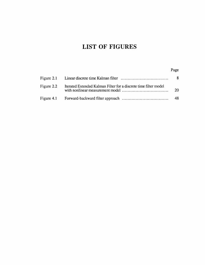
Figure 2.1
Figure 2.2
Figure 4.1
LIST OF FIGURES
Page
Linear discrete time Kalman filter . . . . . . . . . . . . . . . . . . . . . . . . . . . . . . . . . . . 8
Iterated Extended Ka1man Filter for a discrete time filter model with nonlinear measurement model . . . . . . . . . . . . . . . . . . . . . . . . . . . . . . . . . . 20
Forward-backward filter approach . . . . . . . . . . . . . . . . . . . . . . . . . . . . . . . . . . 48
ACKNOWLEDGEMENTS
This technical report was written while the author was on leave from the Faculty of
Geodesy, Delft University of Technology, Delft, The Netherlands. I would like to
thank Dr. David Wells for the hospitality enjoyed during my stay at the Department of
Surveying Engineering at the University of New Brunswick (UNB). Furthermore I
would like to thank my fellow graduate students at UNB for the interest shown in my
work.
Financial assistance for this work was provided by a Strategic Grant entitled
"Marine Geodesy Applications" from the Natural Sciences and Engineering Research
Council of Canada, held by David Wells. Assistance was also provided by Delft
University of Technology.
Vll

SOME ASPECTS OF KALMAN FILTERING
1. INTRODUCTION
The past decades have shown a considerable increase in the number of applications
where a real-time estimate of position is required for a user in a so-called kinematic
mode. Especially in the offshore environment, the demand for precise position and
velocity estimates for a kinematic user has been growing constantly. Kinematic means
that the point to be positioned is actually moving. If one also takes into account the
forces underlying this movement one generally speaks of dynamic positioning. Most
applications of kinematic positioning are found in marine environments (e.g.,
hydrography, seismic surveys, navigation), but also in land surveying kinematic
methods are increasingly put into use (e.g., inertial surveying, motorized levelling,
real-time differential GPS). In this report we have no specific kinematic positioning
application in mind. Actual applications are described in an accompanying report
[Salzmann, 1988].
This report mainly deals with aspects of the estimation process most frequently
used in kinematic and dynamic positioning, namely the Kalman filter. Kalman
filters have been used successfully for years for positioning related problems, which is
mainly due to their convenient recursive formulation which enables an efficient
solution for time varying systems. The concepts and characteristics of Kalman filters
have been discussed extensively since its original inception [Kalman, 1960]. The
Kalman filter is covered in numerous textbooks (e.g., Jazwinski [1970], Gelb
[1974], Anderson and Moore [1979], Maybeck [1979; 1982]). Generally the term
filter is used for all estimation procedures in time varying systems. Actually filtering
Chapter 1: Introduction Page: 1

SOME ASPECTS OF KALMAN FILTERING
encompasses the topics of prediction, where one predicts the state of a system at some
future time; filtering (in the strict sense), where the state of a system is estimated using
all information available at a certain time; and smoothing, where the state is estimated
for some moment in the past. The so-called state of a system constitutes a vector of
parameters which fully describes the system of interest (e.g., a moving vehicle).
In this report some specific aspects of Kalman filters considered relevant for
kinematic positioning problems are discussed. For a general introduction and overall
treatment of the estimation procedures for time varying sytems the reader is referred to
the mentioned textbooks.
In Chapter 2 the discrete time linear Kalman filter and its underlying model are
introduced. The Kalman filter algorithm is derived using a least-squares approach.
Some comments on difficulties in establishing an actual filter model are made.
Chapter 3 is devoted to computational and numerical aspects of Kalman filtering.
The concepts of covariance and inverse covariance (or information) filters are
introduced. Specific implementation methods for the Kalman filter are considered.
Also investigated is which specific method should be used for kinematic positioning
problems.
A general overview of linear smoothing is given in Chapter 4. Smoothing
algorithms are not extensively used in kinematic positioning (a smoothed estimate
hampers real-time applications because of its inherent delay). If a small delay is
acceptable, however, smoothing techniques lead to greatly improved estimates.
The performance analysis of Kalman filters is discussed in Chapter 5. It is very
important that the filter operates at an optimum, because otherwise estimation results
and all conclusions based on them are invalidated. For the performance analysis the
so-called innovations approach is used.
Page:2 Chapter 1: Introduction

SOME ASPECTS OF KALMAN FILTERING
Finally a summary of results is presented in Chapter 6.
Chapter 1: Introduction Page: 3

SOME ASPECTS OF KALMAN FILTERING
Page:4 Chapter 1: Introduction
SOME ASPECTS OF KALMAN FILTERING
2. THE LINEAR KALMAN FILTER
2.1 SYSTEM MODEL AND THE LINEAR KALMAN FILTER
In this chapter we introduce and briefly discuss the mathematical model and the
relations of the linear discrete time Kalman filter. We are mainly interested in discrete
time dynamic systems.
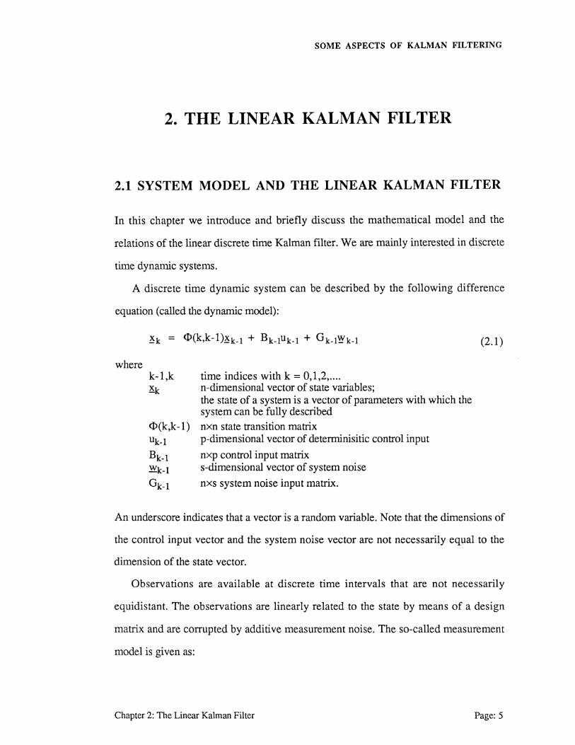
A discrete time dynamic system can be described by the following difference
equation (called the dynamic model):
where k-1,k Kk
<P(k,k-1)
uk-1
Bk-1 wk-1
Gk-1
time indices with k = 0,1,2, .... n-dimensional vector of state variables; the state of a system is a vector of parameters with which the system can be fully described nxn state transition matrix p-dimensional vector of deterrninisitic control input
nxp control input matrix s-dimensional vector of system noise
nxs system noise input matrix.
(2.1)
An underscore indicates that a vector is a random variable. Nate that the dimensions of
the control input vector and the system noise vector are not necessarily equal to the
dimension of the state vector.
Observations are available at discrete time intervals that are not necessarily
equidistant. The observations are linearly related to the state by means of a design
matrix and are corrupted by additive measurement noise. The so-called measurement
model is given as:
Chapter 2: The Linear Kalman Filter Page: S
SOME ASPECTS OF KALMAN FILTERING
(2.2)
where Yk m-dimensional vector of observations
Ak mxn design matrix ~k m-dimensional vector of measurement noise.
Before we proceed, the statistical model underlying the system and measurement
model is specified. The (s-dimensional) vector random system noise and the (m-
dimensional) vector random measurement noise sequences are assumed to be zero
mean, Gaussian, and uncorrelated. Hence:
E{wiJ = 0 E{w· w·t} = Q·O·· -1'-J l lJ E{.~iJ = 0 E{e· e·t} = Ro·· -1'-'J 1 1J E{e· w·t} = 0 -1•-J
where E{.} is the expectation operator, and Oij denotes the Kronecker delta (i.e., Oij=l
if i=j, Oij=O otherwise).
The measurement and system noise sequences describe model disturbances and
noise corruption that affect the system but also uncertainty about the model.
Furthermore initial conditions (k=O) have to be specified. The initial state may assume
a specific value, but because this value is generally not known a priori, the initial state
is considered to be a random vector with a Gaussian distribution and the known
statistics:
E{.!Q} = xo E{ (.!Q-x0) (.!Q-x0)t} = P01o .
Finally it is assumed that the system noise and the measurement noise random
sequences are uncorrelated with the initial state.
Page:6 Chapter 2: The Linear Kalman Filter

SOME ASPECTS OF KALMAN FILTERING
E{ (.~.o-xo) wit} for all i=O,l,2, .... .. E{ (~-x0) ~it} for all i=0,1,2, ..... .
The transition matrix ci>(k,k-1), the design matrix Ak, the noise and control input
matrices (Gk_1 and Bk_1 respectively), and the covariance matrices PolO• Qk , and Rk
are assumed to be known.
Depending on the application one might want to obtain an estimate of the state at a
certain time. If the state is estimated for some future time, the process is called
prediction. If the estimate is made using all measurements up to and including the
current moment, one speaks of filtering. If an estimate is made for some time in the
past using measurements until the current moment, the process is called smoothing.
In this chapter we limit ourselves to prediction and filtering. The Kalman filter
process will now be introduced. It basically consists of two parts:
• time update; the prediction of the state vector and its (error) covariance using the system model and its statistics.
• measurement update; the improvement of the prediction (both the state and its (error) covariance) which gives the filtered state.
The time update is given as:
(2.3a)
(2.3b)
whilst the measurement update can be written in the following form
(2.4a)
(2.4b)
(2.4c)
where Kk is the so-called Kalman gain matrix. The indices of the form ilj denote
Chapter 2: The Linear Kalman Filter Page:7
-r
SOME ASPECTS OF KALMAN FILTERING
estimates at time i based on all measurements till time j. The index kik -1 thus indicates
one step predicted values, whereas klk denotes the estimate at time k using all
measurements including Yk·
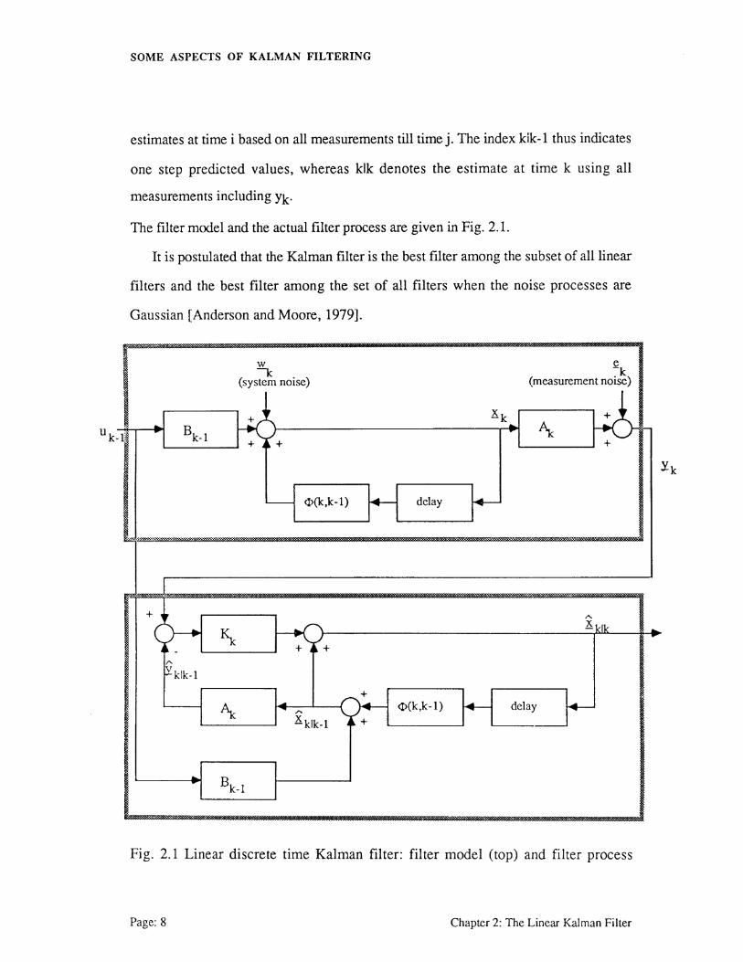
The filter model and the actual filter process are given in Fig. 2.1.
It is postulated that the Kalman filter is the best filter among the subset of all linear
filters and the best filter among the set of all filters when the noise processes are
Gaussian [Anderson and Moore, 1979].
w i<k K (system noise) (measurement noise)
~+ ~ Kk .. Bk-1
· ... t\ ... +
.....___ <l>(k,k-1) r-- delay ...___
'
+ ... "
~ ~ h.?+ Kldk
~ -
~klk-1
t\ ~ 9:-- <l>(k,k-1) ~ delay ~ ,..
Kklk-1
.. Bk-1
Fig. 2.1 Linear discrete time Kalman filter: filter model (top) and filter process
Page: 8 Chapter 2: The Linear Kalman Filter
. .

SOME ASPECTS OF KALMAN FILTERING
(bottom).
2.2 THE LINEAR KALMAN FILTER: A DERIVATION BASED ON LEAST SQUARES
There exist various derivations of the linear Kalman filter. These derivations are based
on principles like least squares, minimum mean square error, maximum likelihood,
and maximum a posteriori. In general the use of different principles leads to different
estimators. However, in the case of linear systems where the probability density
functions are assumed to be Gaussian all the above mentioned estimation methods
yield the same estimator. Thus, the framework used to discuss such systems reduces
to one of personal preference. Since the principle of least squares is probably the one
which surveyors and hydrographers are the most familiar with, our derivation of the
linear Kalman filter in this paragraph is based on this principle. The derivation is taken
from Teunissen and Salzmann [1988]. Other derivatons of the filter process can be
found in, e.g., Jazwinsky [1970], Gelb [1974], Anderson and Moore [1979], and
Maybeck [1979].
The linear model of observation equations from which the linear Kalman filter can
be derived is given as
..... 2Sk-llk-1 I 0
E{ 4k } = -<I>k,k-1 I [ x:~'} ~k 0 Ak
Chapter 2: The Linear Kalman Filter Page: 9

SOME ASPECTS OF KALMAN FILTERING
pk-llk-1
0
0
0 , 0
0
(2.5)
This model is equivalent to the general linear model of the adjustment with
observation equations. Note that in this derivation a deterministic control input is not
taken into account.
The Gaussian random vector ~k-llk-1> with covariance matrix Pk-llk-1• is the
estimator of the state xk_1 at time k-1. It summarizes all the information available at
time k-1 about state xk-1· The Gaussian random vector .dk, with covariance matrix
Qk-1> is the estimator of the difference between the state xk and the propagated state
<I>klk-1xk-1· If one would know the dynamic model perfectly, one would set both the
mean E{dk} and covariance matrix Qk-1 equal to zero. Due to all sorts of random
disturbances, however, in practice one is usually not able to model the dynamics of the
system completely. This is why the difference between the state and propagated state is
modelled as a random vector.
The Gaussian random vector Yk· with covariance matrix Rk, is an estimator of the
observational variates at time k. Its mean is related to the state xk through the design
matrix Ak.
In order to estimate we need sample values. In practice we have only samples
available for Kk-llk-1 and Yk· The sample of Xk-11k-1 is given by the best estimate of xk-1
at time k-1, and the sample of Yk is given by the observations. There is, however, no
sample available for llk· Since the difference between the state and propagated state is
considered to be small, the random vector .dk is treated as a pseudo-observational
variate for which the sample value can be taken equal to zero.
Page: 10 Chapter 2: The Linear Kalman Filter
SOME ASPECTS OF KALMAN FILTERING
Prediction
The least-squares estimation of the state without the use of the observations Yk is
considered first. Model (5) reduces then to
0
I
pk-llk-1
0
Note that there is no redundancy since the model contains 2n equations with 2n
unknowns. Thus the available estimatexk-11k-1 ofxk-1 cannot be improved upon. Due
to the lack of redundancy in (2.6) the least-squares estimator of xk, which we shall
denote by gklk-1> simply follows from inverting the design matrix of (2.6). Thus
"" "" ~klk-1 = Cl>k k-l~k-llk-1 + ~h ' . (2.7)
Application of the error propagation law gives for the covariance matrix ofxklk-1:
(2.8)
Since the sample value of gk is taken equal to zero it follows from (2.7) that the least
squares estimate of xk based on model (2.6) is given by
~klk-1 = Cl>k k-1~k-llk-1 ' . (2.9)
Equations (2.8) and (2.9) constitute the well known time update equation of
the linear Kalman filter. They are equivalent to equations (2.3a) and (2.3b) in section
2.1.
Chapter 2: The Linear Kalman Filter Page: 11

SOME ASPECTS OF KALMAN FILTERING
Filtering
The least squares estimation of the state with the observations Yk included is now
considered. In this case model (2.5) applies. Since there is redundancy (the
redundancy equals the dimension of the vector of observations) the available estimate
~k-11k-1 of xk-1 can now be improved. This improvement is, however, part of
smoothing (i.e., one uses the observations of time k to estimate the state at time k-1)
and is not considered in the Kalman filter. The state xk_1 is therefore eliminated from
model (2.5). This gives
E { [ cl> k,k -1~ ;~11k- ,+Q k] } ~ [ ~J k { cl>k.k _,P k-llk-1cl>~.: 1 +G k-1<4-1G ~ -1 :J (2.10)
With (2.7) and (2.8) this can also be written as
(2.11)
Straightforward application of the least-squares algorithm gives for the least-squares
estimator of xk, denoted by Xklk:
(2.12)
Application of the error propagation law gives for the covariance matrix ofKklk:
(2.13)
Equations (2.12) and (2.13) constitute the so-called measurement update
equations of the linear Kalman filter. An alternative form of the measurement update
Page: 12 Chapter 2: The Linear Kalman Filter
SOME ASPECTS OF KALMAN FILTERING
equations can be obtained by invoking the following matrix inversion lemma:
(2.14)
where C and D are symmetric matrices. The identity (2.14) is easily verified by
multiplying the right-hand side of (2.14) with [C-l+Btn-lB]. Application ofthe matrix
inversion lemma (2.14) to (2.12) and (2.13) gives after some arrangements for the
filtered state
(2.15)
and for its covariance matrix
(2.16)
The measurement update equations (2.15) and (2.16) are the ones which are
usually presented in the literature. They are given as equations (2.4b) and (2.4c) in
section 2.1.
2.3 EXTENSIONS OF THE SYSTEM MODEL
Now the Kalman filter has been established, a few remarks regarding the properties of
the filter and possible extensions to the filter concept can be made.
2.3.1 Alternative System Models
The dynamic model on which the Kalman filter is based has been introduced as a
discrete time linear dynamic system. Such a discrete time system can often be derived
directly for the problem at hand. In many cases, however, such a system is based on a
Chapter 2: The Linear Kalman Filter Page: 13
SOME ASPECTS OF KALMAN FILTERING
continuous time dynamic system. Especially if one wants to describe the dynamics
(e.g., forces) underlying the model, the system model can often be better represented
as
i(t) = F(t)~(t) + B(t)u(t) + G(thy(t) (2.17)
which is a linear differential equation with one independent variable (in our case time t)
and where
. d x(t) = dt x(t) •
F(t) is the so-called nxn dynamics matrix. An initial condition !(to)=xo is
assumed. It is assumed that the measurement model is based on sampled
measurements and thus the measurement model remains unchanged.
The Gaussian process w(t) is an m-dimensional Gaussian process of zero mean
and strength Q(t).
E{~(t))} = 0 E{ w(t) w(s)t } = Q(t)8(t-s)
where Q(t) is a spectral density matrix [Gelb, 1974].
Given model (2.17) the time update equations can be solved in continuous time.
Using numerical integration techniques a solution for the system state
iCt) = F(t)~(t) + B(t)u(t) (2.18)
can be obtained starting from the initial value xo and its covariance matrix can be
computed. The update equation for the covariance is not derived (see e.g. Gelb
[1974]) and is given here for easy reference:
P(t) = F(t)P(t) + P(t)F(t) t + G(t)Q(t)G(t) t (2.19)
(starting from the initial value P0).
Page: 14 Chapter 2: The Linear Kalman Filter
SOME ASPECTS OF KALMAN FILTERING
Although it might be advantageous to formulate the dynamic model in continuous
time it is indicated how the discrete time equivalent of model (2.17) can be obtained.
This enables us to perform the actual processing with the previously outlined discrete
time algorithm.
The solution of the differential eqn. (2.17) is given by:
~(t) = <l>(t,to)x0 + ft<l>(t;t)B('t)u('t)dt + ft<l>(t,'t)G('t)W('t)d't to to (2.20)
Although the last term in eqn. (2.20) cannot be evaluated properly, this imprecise
notation will be maintained (for a discussion see Maybeck [1979]). By inserting the
proposed solution in eqn. (2.17) it can be seen that this is a valid solution. <l>(t,to) is
the state transition matrix that satisfies the differential equation
d dt(<l>(t,t0)) = F(t)<l>(t,t0)
and the initial condition
<I>(t0,t0) = 1 .
The transition matrix has the following property:
and thus
<l>(t,t0)<l>(t0,t) = <l>(t,t) = I
so that -1
<l>(t,t0) = <I>( to. t) .
If the dynamics matrix F(t) is a constant matrix (i.e., F(t)=F for all t) the transition
matrix <l>(t,to) is a function of the time difference (t-to) only. The transition matrix can
then be expressed as a matrix exponential
Chapter 2: The Linear Kalman Filter Page: 15

SOME ASPECTS OF KALMAN FILTERING
Cl>(t,to) = Cl>(t-t0) = eF(t-to)
or by the equivalent series expansion
oo (t-to)~n Cl>(t-to) = L '
0 n. n=
In the case of time invariant systems the transition matrix Cl>(t-to) can also be obtained
via the inverse Laplace transform
-1 -1 Cl>(t-t0) = £ (si - F) .
The derivation via Laplace transforms can be very advantageous for analytical studies.
To summarize how the state transition matrix can be obtained is by numerical
integration methods and in the time invariant case by a matrix series expansion or
using Laplace transforms.
If one assumes that the control input u(t) is constant between two measurement
updates it follows that
The term
is equivalent to Gk-1wk-1 in eqn. (2.1) although it cannot be evaluated rigorously.
Now that the time update of the state has been linked to the discrete time model the
state covariances are discussed. In continuous time
t t E{ (G('t)W('t))(G(cr)~(cr)) } = G('t)Q('t)G('t) O('t-cr)
Page: 16 Chapter 2: The Linear Kalman Filter
SOME ASPECTS OF KALMAN FILTERING
The discrete time formulation can be derived as follows:
which by taking the expectation operator into the integral signs and recalling the
definition of the continuous time system noise can be written as:
Note that Qk-l is a covariance matrix. Gk-lQk-lGk-lt is not necessarily positive
definite, but always semi-positive definite. Furthermore it holds that
Starting from a continuous time dynamic system model it has been shown how the
discrete time equivalent form can be obtained.
2.3.2 Model Nonlinearities
Until now we have assumed a linear dynamic model and a linear measurement model.
In practice, however, often nonlinear models are encountered. Although the linear
model will not provide a valid description anymore (i.e., the nonlinearities in the
model are not negligible) we still want to exploit the linear estimation concepts derived
earlier, and thus apply the developed linear estimation results.
In general both the dynamic model and the measurement model can be nonlinear. A
continuous time nonlinear system can, e.g., be formulated as:
~(t) = f(A(t),u(t),t) + G(thy(t) (2.21)
Chapter 2: The Linear Kalman Filter Page: 17
SOME ASPECTS OF KALMAN FILTERING
where f is a known n-vector of functions of three arguments. Note that the dynamic
system noise (iy(t)) enters in a linear additive fashion. This does not generally hold
true. The measurement model is still based on sampled measurements. The nonlinear
measurement model is decribed by
(2.22)
with ~ as defined earlier.
Note that also in this case the noise enters in a linear additive fashion. In many
applications in surveying and hydrography the system dynamic model can be modelled
adequately as being linear. The measurement model, however, will usually be
nonlinear. A method to deal with nonlinearities in the model is to use a first-order
approximation. Then the measurement model can be expanded in a Taylor series
(neglecting the higher-order terms):
where
The design matrix obtained by linearization can then be used in the Kalman filter
measurement update equations presented earlier.
One can linearize the measurement function about different points. If some nominal
trajectory is available and linearization is done about points of this trajectory, the filter
process is called a linearized Kalman filter (LKF). If the linearization is done about the
predicted state estimate (i.e., xkO = xklk- 1) the process is called an extended Kalman
filter (EKF). If the solution is iterated (until a certain stopping criterion is met) using
Page: 18 Chapter 2: The Linear Kalman Filter
SOME ASPECTS OF KALMAN FILTERING
the most recent state estimate (starting with the predicted state), the process is called an
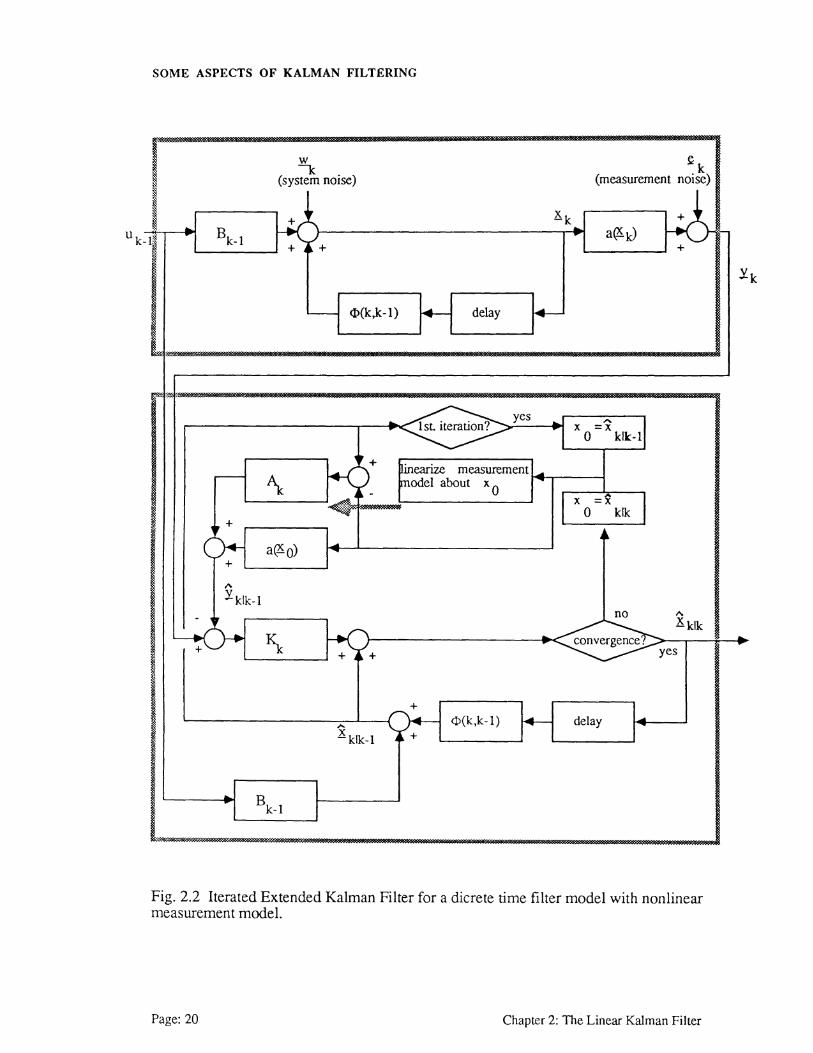
iterated extended Kalman filter (lEKF). See Fig. 2.2
In the case of an lEKF the measurement update equation for the system state can
be written as:
iklk,(i+1) = iklk-1 + Kk,(i)(Yk- ak(iklk,(i~- Ak,(i)(iklk-1- iklk,(i~)
where i denotes the number of iterations.
Apart from this the lEKF equations are equivalent to those of the linear Kalman
filter. Due to the iterative nature, the computational burden of the lEKF may be much
larger than that of the linear Kalman filter. The lEKF is probably the most frequently
used method in hydrography and surveying to deal with nonlinearities in the filter
model.
2.3.3 Filter Design Considerations
If the Kalman filter model is linear, the Kalman filter process equations show that the
propagation and update equations of the (error) covariance matrix of the system state
and the Kalman gain matrix are independent of the actual observations. Thereby the
opportunity is given to perform an a priori accuracy analysis of the Kalman filter
performance
In case the filter model is time invariant the filter will operate in steady state
conditions after some time. This facilitates the assessment of the filter accuracy for the
whole period of interest by only analyzing a single steady state sample. Even in case
the filter model is nonlinear, however, an a priori accuracy analysis is not impossible.
Chapter 2: The Linear Kalman Filter Page: 19
-
SOME ASPECTS OF KALMAN FILTERING
w ~k 1c . ) (system nOise (measurement noise)
I ~+ ~ xk ... Bk-1
• a~0 : +
L-- <l>(k,k-1) ~ delay ~
..
1st iteration? yes
x o =xktk-1!
.+
k ~earize measurement .-- '\ ~odel about xo ... j~- ...
I X =X ""'4> 0 klk
r+
>:- ~ ~
a(Xo)
,.. Yktk-l
no ,.. -Xktk
~ ~ k) .. convergence·! + j~ + yes
o.- <t>(k,k-1) ..__ delay ..... ..... xktk-1 +
. Bk-1
Fig. 2.2 Iterated Extended Kalman Filter for a dicrete time filter model with nonlinear measurement model.
Page: 20 Chapter 2: The Linear Kalman Filter
y k
...
SOME ASPECTS OF KALMAN FILTERING
Assuming a nominal trajectory the update and propagation equations for the (error)
covariance can be performed without the actual measurements being available. The
obtained results will, however, only be approximate.
2.3.4 Alternative Noise Models
The Kalman filter described in this chapter is based on the fact that the system noise
and measurement noise sequences are white and mutually uncorrelated. These results
can be extended by allowing correlation between both noise sequences. If one assumes
a correlation between the measurement noise at time k and the dynamic system noise of
the ensuing sample period the statistical model is expanded as:
E { wk~jt } = Skokj .
Allowing this correlation leaves the Kalman filter measurement update unchanged. The
equations of the time update change however (see Maybeck [1979, p.246], Anderson
and Moore [1979, p.108]).
If on the other hand one assumes correlation between the system noise over a
sample period and the noise corrupting the measurement at the end of the sample
interval, which can be stated as:
then the time update equations remain unchanged, but the equations of the
measurement update are slightly different (see Maybeck [1979, p.247]).
Exploiting the correlation between system noise and measurement noise improves
the estimation precision. Probabilistic information on the realization of the system
noise is obtained by the observation of the particular realizations of the measurement
Chapter 2: The Linear Kalman Filter Page:21
SOME ASPECTS OF KALMAN FILTERING
noise [Maybeck, 1979]. In practice it might be difficult, however, to specify a realistic
S-matrix.
Another possible extension to the statistical model is the assumption that the noise
sequences are not white. The noise models can then be developed further in state space
models and thereby lead to state augmentation. State augmentation is the most
generally applied technique in this case. State augmentation can increase the
computational load of the Kalman filter process considerably.
Sometimes models for the measurement noise can be developed (e.g., the
measurement noise sequence is a Markov process, that is, the realization of the noise
process at certain time depends only on the realization of that process at the previous
moment and a random input). This setup is equivalent to a measurement free problem
and is not discussed here any further.
2.4 FINAL MODEL CONSIDERATIONS
In this chapter some aspects of the discrete time linear Kalman filter and its underlying
model have been discussed. In the subsequent chapters some specific aspects of the
Kalman filter will be investigated, which are basically unrelated to the exact structure
of the filter model. Therefore a somewhat simplified model will be used for further
investigations.
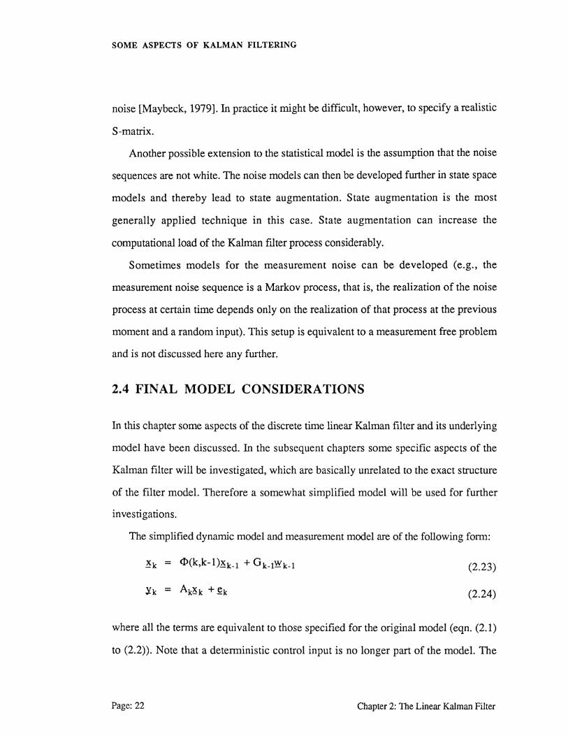
The simplified dynamic model and measurement model are of the following form:
~k = <l>(k,k-l)~k-1 + Gk-1Wk-1
~k = Ak~k + ~k
(2.23)
(2.24)
where all the terms are equivalent to those specified for the original model (eqn. (2.1)
to (2.2)). Note that a deterministic control input is no longer part of the model. The
Page:22 Chapter 2: The Linear Kalman Filter

SOME ASPECTS OF KALMAN FILTERING
derived Kalman filter time and measurement update equations remain unchanged
provided that the deterministic control input is deleted.
Chapter 2: The Linear Kalman Filter Page:23

SOME ASPECTS OF KALMAN FILTERING
SOME ASPECTS OF KALMAN FILTERING
3. COMPUTATIONAL CONSIDERATIONS
3.1. INTRODUCTION
In the previous chapter the linear Kalman filter was introduced. Time update and
measurement update equations were derived for the linear Kalman filter. There exist,
however, a range of different algorithms, generally called mechanizations. In the
sixties and early seventies limited computer core memory size and low computing
speeds led to the development of various mechanizations. Theoretically all these
mechanizations lead to identical results. It was found, however, that if single precision
arithmetic was used for the implementation of certain filter mechanizations, numerical
problems could arise during the filter computations. Therefore numerous
investigations concerning these numerical problems were set up. These investigations
were mainly related to aerospace problems. In this context numerical properties and the
computational efficiency of almost all mechanizations have been investigated.
It is of interest up to what extent numerical problems will arise in kinematic
positioning problems (and the closely related field of navigation) and which
mechanization should be preferred. In this chapter we will review the two basic forms
of Kalman filter mechanizations and we will investigate which mechanizations are best
suited for our purposes.
This chapter only addresses the computational aspects directly related to the
different filter mechanizations of the linear Kalman filter. If, as often occurs in
practice, the design, transition, and covariance matrices are not known (e.g., in case of
nonlinearities of the model) the computational burden of computing these matrices can

SOME ASPECTS OF KALMAN FILTERING
account for up to 90% of the total computational burden of the Kalman filter. As is it
likely that these computations have to be performed for every mechanization,
compuational aspects not directly related to a specific mechanization are not considered
here.
In section 3.2. the concepts of the covariance and inverse covariance (or
information) filters are introduced. Section 3.3. is devoted to square root filtering,
where the square root of the covariance matrix of the state (rather than the covariance
matrix itself) is propagated in time. In section 3.4 a closer look is taken at the U-D
covariance factorization method which is closely related to the square root concept.
Finally some implementation considerations are discussed in section 3.5.
3.2 BASIC FILTER MECHANIZATIONS
Filter mechanizations can be devided into two major classes. The covariance filters
and the inverse covariance filters. Covariance filters propagate the covariance
matrix of the state in time. Inverse covariance filters propagate the inverse of the
covariance matrix. Inverse covariance filters are usually called information filters.
The covariance-type (standard) Kalman filter equations have been derived in
Chapter 2. The time and measurement update equations of the linear Kalman
(covariance) filter are repeated here for easy reference. The time update equations for
the estimate of the state and its covariance are given as:
xklk-1 = <l>(k,k-l)ik-11k-1 (3.1a)
(3.lb)
SOME ASPECTS OF KALMAN FILTERING
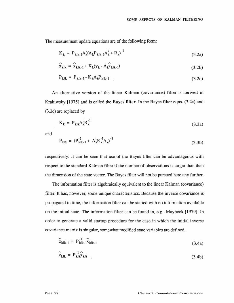
The measurement update equations are of the following form:
(3.2a)
"' "' "' xklk = xklk-1 + Kk(Yk- AiJCklk-1) (3.2b)
(3.2c)
An alternative version of the linear Kalman (covariance) filter is derived in
Krakiwsky [1975] and is called the Bayes filter. In the Bayes filter eqns. (3.2a) and
(3.2c) are replaced by
(3.3a)
and
(3.3b)
respectively. It can be seen that use of the Bayes filter can be advantageous with
respect to the standard Kalman filter if the number of observations is larger than than
the dimension of the state vector. The Bayes filter will not be pursued here any further.
The information filter is algebraically equivalent to the linear Kalman (covariance)
filter. It has, however, some unique characteristics. Because the inverse covariance is
propagated in time, the information filter can be started with no information available
on the initial state. The information filter can be found in, e.g., Maybeck [1979]. In
order to generate a valid startup procedure for the case in which the initial inverse
covariance matrix is singular, somewhat modified state variables are defined.
... -1 "' zklk-1 = Pklk-1xklk-1 (3.4a)
... -1 "' zklk = Pkl0klk (3.4b)
Pa!Ie:27
SOME ASPECTS OF KALMAN FILTERING
With t.... -1
Mk = Cl>(k-l,k) t'k-llk-lci>(k-l,k) (3.5)
the time update equations of the information filter are given as:
(3.6a)
(3.6b)
The measurement update equations of the information filter are:
(3.7a)
(3.7b)
It can be seen from eqns. (3.7a) and (3.7b) that the information filter is more efficient
in computing the measurement update than the covariance filter. On the other hand the
time update equations of the information filter are more complex than those of the
covariance filter. The inverses that have to be computed for the covariance filter
recursions basically depend on the dimension of the observation process, whereas for
the information filter they depend primarily on the dimension of the state vector.
The advantages of covariance filters can be summarized as follows:
• Continuous estimates of state variables and their covariances are available at no extra computational cost.
• Covariance type filters appear to be more flexible and are easier to modify to perform sensitivity and error analysis [Bierman, 1973a].
The advantages of inverse covariance or information filters are:
• Large batches of data (i.e. m>>n) are processed very efficiently from a computational point of view.
Chapter 3: Computational Considerations
SOME ASPECTS OF KALMAN FILTERING
e No information concerning the initial state is required to start the information filter process (i.e., the inverse covariance matrix at the start of the information filter process may be zero).
In general covariance type filters will computationally be more efficient than
information type filters if frequent estimates are required.
In cycling through the filter equations the covariance matrix (or its inverse) of the
state can result in a matrix which fails to be nonnegative positive. The measurement
update of the covariance filter can be rather troublesome numerically. Equation (3.2c)
can involve small differences of large numbers, particularly if at least some of the
measurements are very accurate. It has been shown [Bierman, 1977] that on finite
wordlength computers this can cause numerical precision problems. Therefore an
equivalent form of (3.2c), called the Joseph-form, is often used:
(3.8)
Apart from better assuring the symmetry and positive definiteness of Pkik· the Joseph-
form is also insensitive, to first order, to small errors in the computed filter gain
[Maybeck, 1979]. However, the Joseph-form requires a considerably greater number
of computations than (3.2c). In the literature the Joseph-form is generally called the
stabilized Kalman filter.
For the information filter a stabilized version of the covariance time update
equation (which is anagolous in form to the covariance measurement update of the
covariance filter) exists. This analogue of the Joseph-form for the information filter is
given in [Maybeck, 1979]:
(3.9)
Page:29 Chapter 3: Computational Considerations
SOME ASPECTS OF KALMAN FILTERING
where
3.3 SQUARE ROOT FILTERING
Because the stabilized filter mechanizations required to much storage and computations
for early Kalman filter applications, an alternative strategy to cope with the numerical
problems encountered in computing the (error) covariance matrix was developed. The
limited computer capabilities forced the practitioners to use single precision arithmetic
for their computations, while at the same time numerical accuracy had to be warranted.
It was soon realized that nonnegative definiteness of the covariance matrix could also
be retained by propagating this matrix in a so-called square root form. If M is a
nonnegative definte matrix, N is called a square root of M if M = NNt. The matrix N is
normally square, not necessarily nonnegative definite, and not unique. The matrix N
can be recognized as a Cholesky factor, but the common name "square root" will be
maintained.
Let Sklk and Sklk-1 be square roots of Pklk and Pklk-1 respectively. The product
P=SS1 is always non-negative definite and thus the square root technique avoids
negative definite error covariance matrices.
An overview of different square root filters is given in Chin [1983]. We will
briefly discuss the square root forms of the covariance and information filters. The
presentation of the square root filters is patterned after Anderson and Moore [1979].
Chapter 3: Computational Considerations Page:30
SOME ASPECTS OF KALMAN FILTERING
3.3.1 Square Root Covariance Filter
The time update equations of the square root covariance filter can be summarized as:
iklk-1 = <I>(k,k-1)ik-11k-1 (3.10a)
[ s~lk-1] = T [ s~-11k-1<I>(k,k-1) 1] 0 1 (Q1/2.. bt
k-1) k-1 (3.10b)
In general the matrix T1 can be any orthogonal matrix (i.e. T1T1t =T1tT1=I) making
Sklk-lt upper triangular. In square root implementations the square rootS is chosen to
be the Cholesky factor of P. The measurement update equations of the square root
covariance filter can be represented as:
(3.11a)
s~~kl ]
(3.llb)
with T2 orthogonal.
We will not dwell on the problems concerning the construction of the orthogonal
matrices T1 and T2. Methods suggested in the literature ([Kaminski et al., 1971;
Bierman, 1977; Thornton and Bierman, 1980]) are closely related to well known
stable orthogonalization methods as the Householder and Givens transformations or
the modified Gram-Schmidt orthogonalization scheme. It is due to these numerically
stable orthogonalization methods that square root filters show improved numerical
Page: 31 Chapter 3: Computational Considerations
SOME ASPECTS OF KALMAN FILTERING
stability. Square root filters show better numerical behaviour in computing covariance
matrices than the standard Kalman filter. As far as error analysis is concerned this
cannot be claimed for the gain matrix (K) or the estimate itself (x) (see LeMay [1984]
and Verhaegen and van Dooren [1986]). For a more extensive treatment of square root
covariance filters the reader is referred to Anderson and Moore [1979] and Maybeck
[1979].
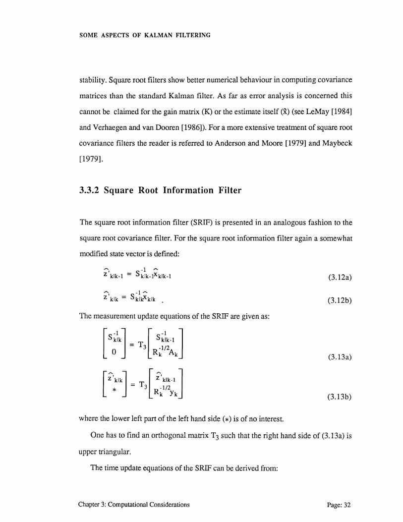
3.3.2 Square Root Information Filter
The square root information filter (SRIF) is presented in an analogous fashion to the
square root covariance filter. For the square root information filter again a somewhat
modified state vector is defmed:
"" 1 "" z 1klk-1 = sklk-1xklk-1 (3.12a)
"", -1 "" z klk = skl0klk (3.12b)
The measurement update equations of the SRIF are given as:
(3.13a)
[ ~·klk] = T [ ~·klk-1] * 3 R-1/2
k Yk (3.13b)
where the lower left part of the left hand side ( *) is of no interest.
One has to find an orthogonal matrix T 3 such that the right hand side of (3.13a) is
upper triangular.
The time update equations of the SRIF can be derived from:
Chapter 3: Computational Considerations Page:32

SOME ASPECTS OF KALMAN FILTERING
]=
[ (Q~~~ -1
T4 -1 S k-llk-1<l>(k-1 ,k)Gk-1
0 ] (3.14a)
-1 s k-11k-l<l>(k-1,k)
with Mk as defined in (3.5).
Once again the general idea is to find an orthogonal matrix (T4) such that the right
hand side of (3.14a) is upper triangular and with this T4 one finds:
[ * J [ 0 J "' = T4 ,..... z'klk-1 z'k-llk-1 (3.14b)
The square root information filter (SRIF) is covered extensively in Bierman [1977]. A
large class of square root mechanizations for both covariance and information filters
has been developed. These are not included here. For an overview the reader is
referred to Chin [1983].
3.4 U-D COVARIANCE FACTORIZATION FILTER
A different approach to square root covariance filters is the so-called U- D
covariance factorization filter developed by Bierman [1977]. The covariance
matrix is not decomposed into square root factors, but in the form UDUt, where U is a
unitary upper traingular (i.e., with ones along the diagonal) and D is a diagonal matrix.
The U-D covariance factorization filter (or U-D filter) is basically an alternative
Page: 33 Chapter 3: Computational Considerations

SOME ASPECTS OF KALMAN FILTERING
approach to the classical square root filters (see, e.g., Kaminski et al. [ 1971 ]). The
factors U and D are propagated in time. For the U-D factorization the covariance
matrices of the predicted and filtered state are factored as:
(3.15a)
(3.15b)
The close relationship of the U-D filter with square root filters is apparent, because
uol/2 corresponds directly to a covariance square root. The main advantage of the U
D filter algorithm over the conventional square root filters is that no explicit square root
computations are required. At the same time the U-D factorization shares the
favourable numerical characteristics of the square root methods. If a matrix is positive
(semi) definite a U-D factor can always be generated. The algorithm of the U-D
factorization is closely related to the backward running Cholesky decomposition
algorithm and is given in Appendix I.
3.4.1 U-D Filter Measurement Update
The U-D filter measurement updates are performed component wise and hence scalar
measurement updates are used. If more than one observation per update is available,
the measurements are processed sequentially. If the covariance matrix of the
observations (Rk) is originally not diagonal, the measurement variables have to be
transformed first in order to be able to apply this algorithm. If the covariance matrix of
the observations is non-diagonal the Cholesky decomposition of Rk into a lower
triangular matrix (i.e., Rk = LkLk1) is computed first. Then the measurement model
¥k = Akxk+ ~k
Chapter 3: Computational Considerations Page:34

SOME ASPECTS OF KALMAN FILTERING
is converted to
* * * ~k = Ak~k+~k
where
* LI&k = ~k
It then follows that
* *t E{~k~k} = I .
After this transformation of variables the U-D filter measurement update can be used.
Starting from the linear Kalman (covariance) filter measurement update equations of
the covariance we fmd for a scalar measurement update:
(3.16)
where
This form can be factored as (given the U-D factor ofPklk-1):
Defming the vectors f and v (both of dimension n) as
and substituting these in (3.17) yields:
Page: 35 Chapter 3: Computational Considerations

SOME ASPECTS OF KALMAN FILTERING
(3.18)
The part in parentheses in (3.18) is positive (semi) definite and can therefore be
factored as UDUt. Furthermore the product of two unitary upper triangular matrices is
again unitary upper triangular so that (3.18) can be written as:
(3.19)
where u klk = u klk-lu
It can be seen that the construction of the updated U-D factors depends on the simple
factorization
----t t UDU = Dklk-l- (1/a)vv (3.20)
The U-D factors can be generated recursively [Bierman, 1977]. In practical
implementations of the measurement update of the U-D filter the Kalman gain matrix is
not computed explicitly, but if desired it can be computed at very little extra
computational cost. An algorithm for computing the U-D filter measurement update is
given in Appendix I.
3.4.2 U -D Filter Time Update
For the time update of the U -D filters two methods are in use. The most trivial one is
to "square up" the U-D factor to obtain the time propagated error covariance:
Chapter 3: Computational Considerations Page:36
SOME ASPECTS OF KALMAN FILTERING
The matrix Pklk-1 can then be factored into Uklk-1 and Dklk-1 using the U-D
factorization algorithm. This procedure is thought to be a stable process. Numerical
difficulties can arise, however, if <I>(k,k-1) is large or Pklk-1 is ill conditioned
[Thornton and Bierman, 1980]. An advantage of the above method is that the
covariance matrix of the (predicted) state is readily available.
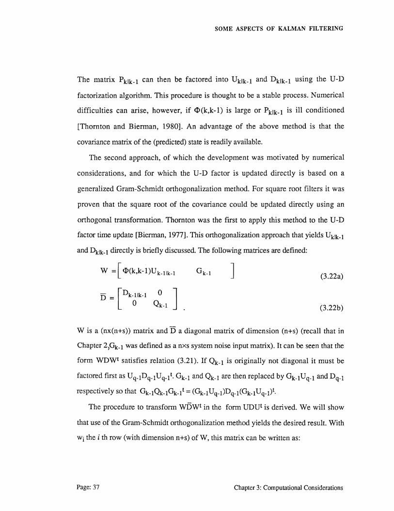
The second approach, of which the development was motivated by numerical
considerations, and for which the U-D factor is updated directly is based on a
generalized Gram-Schmidt orthogonalization method. For square root filters it was
proven that the square root of the covariance could be updated directly using an
orthogonal transformation. Thornton was the first to apply this method to the U-D
factor time update [Bierman, 1977]. This orthogonalization approach that yields Uklk-1
and Dklk-1 directly is briefly discussed. The following matrices are defined:
W = [ <l>(k,k-1)Uk-llk-l J (3.22a)
D = [Dk-llk-1 0 J 0 Qk-1 (3.22b)
W is a (nx(n+s)) matrix and D a diagonal matrix of dimension (n+s) (recall that in
Chapter 2,Gk-l was defined as a nxs system noise input matrix). It can be seen that the
form WDWt satisfies relation (3.21). If Qk_ 1 is originally not diagonal it must be
factored first as Uq-1Dq-1 Uq_{ Gk-1 and Qk-1 are then replaced by Gk-1 Uq_1 and Dq_1
respectively so that Gk_1Qk-1Gk_1t = (Gk_1Uq_1)Dq-1(Gk-1Uq_1)t.
The procedure to transform w:i5wt in the form UDUt is derived. We will show
that use of the Gram-Schmidt orthogonalization method yields the desired result. With
withe i throw (with dimension n+s) of W, this matrix can be written as:
Page: 37 Chapter 3: Computational Considerations

SOME ASPECTS OF KALMAN FILTERING
W=
(3.23)
An orthogonal basis of vectors {v1, .... ,vn} is constructed applying the Weighted
Gram-Schmidt (WGS) orthogonalization method to the rows of the matrix W
(3.24)
-f (wpvJ ·-vj = wj- ~ t- vk , J-n-1, ... ,1
k=j+l(vkDv0
The algorithm defmed here is given in a backward recursive form, because the result is
needed to construct an upper triangular matrix factorization. We can now define an
orthogonal matrix T:
(3.25)
The vectors v1, .... ,vn are computed using the WGS procedure. The remaining s
columns of T are additional orthogonal basis vectors (of dimension n+s) which,
however, do not have to be computed explicitly. We can write the matrix product of
the matrices Wand T as:
Wf=
(3.26)
Chapter 3: Computational Considerations Page:38
SOME ASPECTS OF KALMAN FILTERING
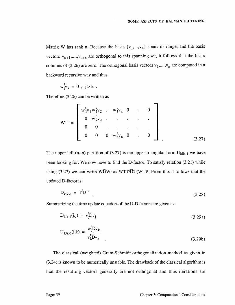
Matrix W has rank n. Because the basis {v~o ... ,v0 } spans its range, and the basis
vectors Vn+lo .... ,vn+s are orthogonal to this spanning set, it follows that the last s
columns of (3.26) are zero. The orthogonal basis vectors v1, .... ,v0 are computed in a
backward recursive way and thus
w }v k = 0 , j > k .
Therefore (3.26) can be written as
WT=
t t WtVtWtVz
t 0 w 2v 2
0 0
0 0
0
0 (3.27)
The upper left (nxn) partition of (3.27) is the upper triangular form Uklk-1 we have
been looking for. We now have to find the D-factor. To satisfy relation (3.21) while
using (3.27) we can write wDWt as WTTtDT(WT)t. From this it follows that the
updated D-factor is:
Dklk-1 = TDT (3.28)
Summarizing the time update equationsof the U-D factors are given as:
(3.29a)
u klk-l(j,k)
(3.29b)
The classical (weighted) Gram-Schmidt orthogonalization method as given in
(3.24) is known to be numerically unstable. The drawback of the classical algorithm is
that the resulting vectors generally are not orthogonal and thus iterations are
Page: 39 Chapter 3: Computational Considerations
SOME ASPECTS OF KALMAN FILTERING
necesssary. Actual implementations are based on the so-called Modified Weighted
Gram-Schmidt (M-WGS) orthogonalization method [Kaminski et al., 1971]. TheM
WGS is basically an algebraic re-arrangement of the classical algorithm. The modified
procedure has favourable numerical characteristics. An algorithm for the U-D filter
time update is given in Appendix I.
3.5 IMPLEMENTATION CONSIDERATIONS
Having introduced the covariance and information filters as well as their respective
square root formulations and the U-D covariance factorization filter a choice between
the different mechanizations for the actual implementation has to be made. To justify
the choice of any mechanization its computational efficiency, numerical aspects and
conditions imposed by the specific application have to be taken into account.
3.5.1 Computational Efficiency
A popular way to assess the computational efficiency of different filter mechanizations
is to compare the number of operations (additions, multiplications, divisions, and
square roots) necessary to compute a full filter cycle (one time update and one
measurement update). These comparisons, usually called operation counts, give a
measure of the relative speed of the algorithms. Operation counts for various
mechanizations can be found in Kaminski et.al. [1971], Bierman [1973a,1977],
Maybeck [1979], and Chin [1983].
Chapter 3: Computational Considerations Page:40
SOME ASPECTS OF KALMAN FILTERING
In the literature contradictory computational efficiencies are reported (see, e.g.,
LeMay [1984]). This may be due to the fact that some authors apply special storage
strategies or only use scalar measurement updates. Usually the operation counts only
consider the filter algorithm itself. Operations not directly related to the filter process
(e.g., input/output and bookkeeping logic) are not taken into account. Furthermore the
computation of the transition matrix (<D), the design matrix (A), and the process
covariance matrix (Q) are not considered either. In cases where the filter model is non
linear the computations of these matrices and the necessary iterations may account for
90% of the total cycle time. In many applications a special problem structure can be
exploited, which can reduce the computational burden as well, but this is not
considered in the operation counts.
As we are restricting ourselves to linear models some useful remarks can be made
regarding the computational efficiency of the different mechanizations. Basically the
standard Kalman (covariance) filter algorithm is the simplest to implement and usually
the fastest. The information filters are of computational interest if the dimension of the
measurement vector is larger than the dimension of the state vector. Covariance filters
are more efficient if frequent estimates of the state are required. The stabilized Kalman
filter is computationally always less efficient than the standard Kalman filter by about
10%-50%. Square root covariance filters and U-D filters may be up to 50% slower
than the standard Kalman filter. For certain applications, however, it has been shown
[Thornton and Bierman, 1980] that non-standard mechanizations may be
computationally just as efficient as the standard Kalman filter. In problems where the
dimension of the state vector is small the differences between the various
mechanizations are generally not of great importance, because then for all
mechanizations low operation counts (and thus cycle times) can be obtained.

SOME ASPECTS OF KALMAN FILTERING
3.5.2 Numerical Aspects
Up to now we only dealt with different Kalman filter mechanizations from a
computational point of view. The usefulness of different mechanizations depends,
besides on the computational efficiency, mainly on their numerical stability. It has been
indicated that the equivalence of the square root and U-D factorization algorithms with
the numerically stable Householder and Givens (orthogonal) transformations
guarantees the numerical stability of these mechanizations. It has also been mentioned
that this is only true for the (error) covariance update. Therefore the comparison of
different mechanizations from a numerical point of view is very interesting. Such
comparisons can be found in Thornton and Bierman [1980] and Verhaegen and van
Dooren [1986].
The basic motive for the development of square root related filters was to enable
filter computations in single precision arithmetic (to ease storage requirements and to
speed up the computations). Single precision arithmetic computations are indeed
possible due to the enhanced numerical stability of the square root filters.
It has been shown in Thornton and Bierman [1980] that if computations are
performed in double precision arithmetic, no numerical difficulties are to be
encountered for any mechanization. In these cases the mechanization with the highest
computational efficiency (which is not necessarily the standard Kalman filter) can be
selected for the computations.
When computing with single precision arithmetic one will always encounter some
numerical degradation compared to the double precision computations [Thornton and
Bierman, 1980]. With the use of the square root or U-D filters only limited
Chapter 3: Computational Considerations P:u:r~: .4?.
SOME ASPECTS OF KALMAN FILTERING
degradation will occur. Thornton and Bierman also encountered numerical instability
using the stabilized Kalman Filter with single precision arithmetic. On the other hand
Verhaegen and van Dooren [1986] show, by means of a theoretical error analysis, that
square root formulations and the stabilized Kalman filter should have the same
numerical accuracy.
3.5.3 Practical Considerations
For practical applications special characteristics of the problem can often be exploited,
such as the sparseness of the transition or covariance matrices (which are often
reduced to diagonal form). In applications the state transition matrix has often a (block)
triangular form. Exploiting these characteristics can lead to considerable computational
savings.
In the investigation of Kalman filter mechanizations we dealt primarily with linear
time varying systems. In some applications the Kalman filter may reach (after an initial
transient period) a (almost) steady state condition. The computation of the gain matrix
is the largest computational burden of the Kalman filter algorithm. The use of a steady
state gain can lead to considerable computational savings. Even in time varying
systems this not always leads to a serious performance degradation of the filter
(although the filter will be suboptimal). In such cases an extensive a priori sensitivity
analysis (see Gelb [1974]) is mandatory. An interesting application of the use of a
temporary steady state gain matrix in a navigation environment is discussed by
Upadhyay and Damoulakis [1980] and Gylys [1983].
Exploiting special characteristics of the problem at hand will always reduce the
computational burden, irrespective of the mechanization used. Not considering the
Page:43 Chapter 3: Computational Considerations

SOME ASPECTS OF KALMAN FILTERING
problem characteristics has as advantage that readily available filter routines can be
used in implementing a Kalman filter.
3.5.4 Filter Mechanizations for Kinematic Positioning
In kinematic positioning and navigation frequent updates of the state vector and its
covariance matrix are needed. In a navigation environment the use of covariance filters
seems to be the most appropriate.
The use of the standard Kalman filter in (integrated) navigation systems at sea is
very common. Mostly the standard Kalman filter mechanization is implemented. As
long as the computations are performed in double precision arithmetic numerical
problems are not likely to be encountered. An investigation of navigation filters which
deals with numerical considerations is, e.g., Ayers [1985]. Ayers concludes that for
his simple positioning problem (position a ship with two lines of position (ranges))
special numerical techniques are not necessary and the standard Kalman filter performs
well.
The most popular square root related covariance filter at the moment is the U-D
filter. The U-D filter is very well documented [Bierman, 1977; and Thornton and
Bierman, 1980]. This mechanization is computationally very efficient. It is actually the
computationally most efficient square root related covariance filter mechanization.
When using single precision arithmetic the results are only slightly worse than the
standard Kalman filter results computed with double precision arithmetic. If computer
burden is to be minimized or the computations can only be performed in single
precision arithmetic (e.g., when programming in PASCAL) the U-D factorization
Chapter 3: Computational Considerations Page:44

SOME ASPECTS OF KALMAN FILTERING
mechanization seems to be the most efficient alternative algorithm for navigation
problems.
Page:45 Chapter 3: Computational Considerations

SOME ASPECTS OF KALMAN FILTERING
Chapter 3: Computational Considerations Page: 46
SOME ASPECTS OF KALMAN FILTRERING
4. LINEAR SMOOTHING
4.1 INTRODUCTION
In Chapter 2 we dealt with the concepts of prediction and filtering. We now focus our
attention on the case where one wants to obtain an optimal estimate of the system state
in the past, using measurements both before and after the time of interest. This is the
so-called smoothing problem. Although smoothing has been defined earlier the
definition found in Gelb [1974] is repeated here: "Smoothing is a non-real-time data
processing scheme that uses all measurements between to and tN to estimate the state
of a system at a certain time tk, where to ~ tk ~ tN ".
Because smoothing algorithms use data after the time for which the state is
estimated a time delay in the estimation process is inevitable. For real-time state
estimation filtering and prediction are therefore the only feasible techniques. For
certain real-time applications in surveying and hydrography, however, a small time
delay in obtaining a state estimate may be acceptable. In these cases a smoothed state
estimate will be preferred as more information is taken into account in computing the
estimate. Especially if for some application the data can be processed in an off-line,
postmisson mode smoothing techniques should be considered. Generally a tradeoff
has to be made between the extra computational burden and time delay related to the
smoothing algorithms and the improved accuracy of a smoothed estimate.
In section 4.2 the principles of smoothing are discussed on the basis of the
forward-backward filter approach In section 4.3 three classes of smoothing problems
are discussed. The concept of smoothability is introduced in section 4.4 and some
Chapter 4: Linear Smoothing Page:47
SOME ASPECTS OF KALMAN FILTERING
comments on the possible use of smoothing techniques in hydrography and surveying
are made.
4.2. PRINCIPLES OF SMOOTHING
4.2.1 Forward-Backward Filter Approach
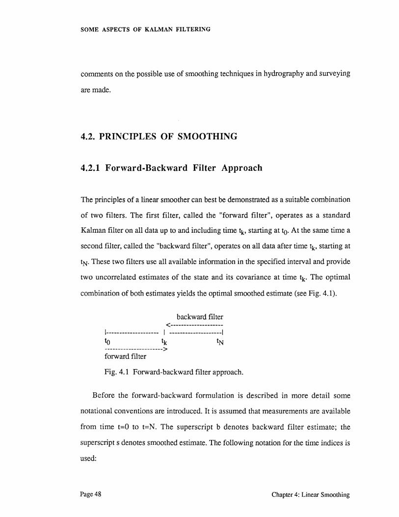
The principles of a linear smoother can best be demonstrated as a suitable combination
of two filters. The first filter, called the "forward filter", operates as a standard
Kalman filter on all data up to and including time tk, starting at to. At the same time a
second filter, called the "backward filter", operates on all data after time tk, starting at
tN. These two filters use all available information in the specified interval and provide
two uncorrelated estimates of the state and its covariance at time tk. The optimal
combination of both estimates yields the optimal smoothed estimate (see Fig. 4.1).
backward filter <:--------------------
1-------------------- I --------------------1 to tk tN ----------------------;> forward filter
Fig. 4.1 Forward-backward filter approach.
Before the forward-backward formulation is described in more detail some
notational conventions are introduced. It is assumed that measurements are available
from time t=O to t=N. The superscript b denotes backward filter estimate; the
superscript s denotes smoothed estimate. The following notation for the time indices is
used:
Page48 Chapter 4: Linear Smoothing

forward filter (01-1) backward filter (010) smoother (0
time
I (010) I (011) I N) I 0
SOME ASPECTS OF KALMAN FILTRERING
(klk-1) (klk)
(k
(klk) (NIN-1) I (NIN) (klk+1) (NIN) I (NIN+1)
I N) (N I N) I ----------------------- I k N
--> <--
A smoothed estimate of the state and its covariance at time tk for data given in the
interval [O,N], where tk is an element of the time interval [O,N], are given as the
optimal combination of two optimal filters [Gelb, 1974]:
(4.1a)
-1 -1 s -1 b
pkiN = pklk + pklk+1 (4.1b)
Given that the forward and backward estimates are uncorrelated these equations can
readily be verified using standard adjustment calculus.The equations show that the
forward filter uses all data up to and including time tk , while the backward filter uses
all data after time tk and in the last step is predicted "backward" to time tk· Equation
(4.1b) shows that the covariance of the smoothed estimate is always smaller than or
equal to the covariance of the forward filter. This is one of the motives to perform
smoothing. This result could have been expected since one uses not only data up to
and including time tk , but all available data in a certain interval.
The linear (forward) Kalman filter was derived in Chapter 2. The formulation of
the backward filter is less straightforward. This is mainly due to the starting values of
the backward filter. Equation ( 4.1 b) shows that the error covariance of the smoothed
estimate is always smaller than the error covariance of the forward filter except for the
terminal time tN. It can be seen from eqn. (4.1b) that at time tN the covariance of the
smoothed state is equal to the forward filter covariance as both are conditioned on
Chapter 4: Linear Smoothing Page:49

SOME ASPECTS OF KALMAN FILTERING
exactly the same data. Hence it follows that the a priori covariance of the backward
filter is infinite, i.e., no a priori statistical information is available to start up the
backward filter. Thus
and assuming ~bNIN+ 1 is finite
This means that the backward filter has to be implemented in the inverse
covariance formulation (also called information filter), because the standard Kalman
filter cannot cope with an infmite a priori covariance. The backward inverse covariance
filter formulation is given in Maybeck [1982, pp. 9-10], where also a somewhat
modified algorithm to compute the smoothed estimate from the the forward filter and
the backward filter is given. Brown [1983] circumvents this problem by suggesting
that as long as the a priori backward filter covariance is chosen 10 times as large as the
a priori covariance of the forward filter a time reversed standard Kalman filter can be
used to implement the backward filter. This may be a valid solution for the example
Brown uses, but one can easily devise some smoothing application where this will
lead to serious suboptimality of the backward filter. In general the inverse covariance
formulation, at least for the first backward steps, is to be preferred. Thereafter one can
use the covariance formulation for the backward filter.
The measurement update equations of the covariance form of the backward filter
are given as:
(4.2a)
Page 50 Chapter 4: Linear Smoothing

SOME ASPECTS OF KALMAN FIL TRERING
(4.2b)
(4.2c)
The time update equations of the backward filter are defined as (note the reversed time
order in the transition matrices):
...... b <l>(k,k+ 1)x k+llk+l (4.3a)
(4.3b)
Conceptually the forward-backward formulation of the optimal smoother is the
easiest way to demonstrate the properties of an optimal smoother. For practical
applications other mechanizations are utilized, which will be treated in the next section.
It is apparent that smoothing involves more computational effort than filtering. A
tradeoff between the extra computational cost and the availability of better estimates
has to be made.
The linear smoother has been introduced using a forward-backward filter
formulation. In the literature numerous other derivations can be found. Kailath and
Frost [1968] use the innovations approach. Koch [1982] uses best linear unbiased
estimators in the regression model. Anderson and Moore [1979] employ the technique
of state augmentation. Houtenbos [1982] formulates the smoothing problem as a least
squares adjustment problem. Rauch et al. [1965] use maximum likelihood estimates.
Starting from single-stage and double-stage optimal smoothers Meditch [1969] derives
the smoothing algorithms via algebraic manipulations and induction. An overview of
the development of smoothing theory is given by Meditch [1973].
Chapter 4: Linear Smoothing Page: 51
SOME ASPECTS OF KALMAN FILTERING
4.3 THREE CLASSES OF SMOOTHING PROBLEMS
In the literature three classes of smoothing problems are distinguished. The
classification depends on how the time k (for which an estimate is needed) and the
length of the data interval N are related. The three classes are fixed-interval, fixed
point, and fixed-lag smoothing.
-Fixed-interval smoothing (k variable, N fixed)
Given measurements in a fixed interval from initial time to to final time tN a smoothed
state estimate at time tk, where tk is an element of the time interval [to,tN], is required,
based on all measurements in the interval. This approach is usually followed in off
line processing.
-Fixed-point smoothing (k fixed, N increasing)
Estimate the state at a single fixed point in time tk as more and more measurements
become available after time tk.
-Fixed-lag smoothing (k increasing, N-k fixed)
A smoothed estimate at a fixed time interval back in the past is computed. The
computation of the state estimate at time tk is delayed for a fixed time tlag to take
advantage of the additional information in the interval of duration !Jag (=N-k) of the
most recent measurements.
Page 52 Chapter 4: Linear Smoothing
SOME ASPECTS OF KALMAN FILTRERING
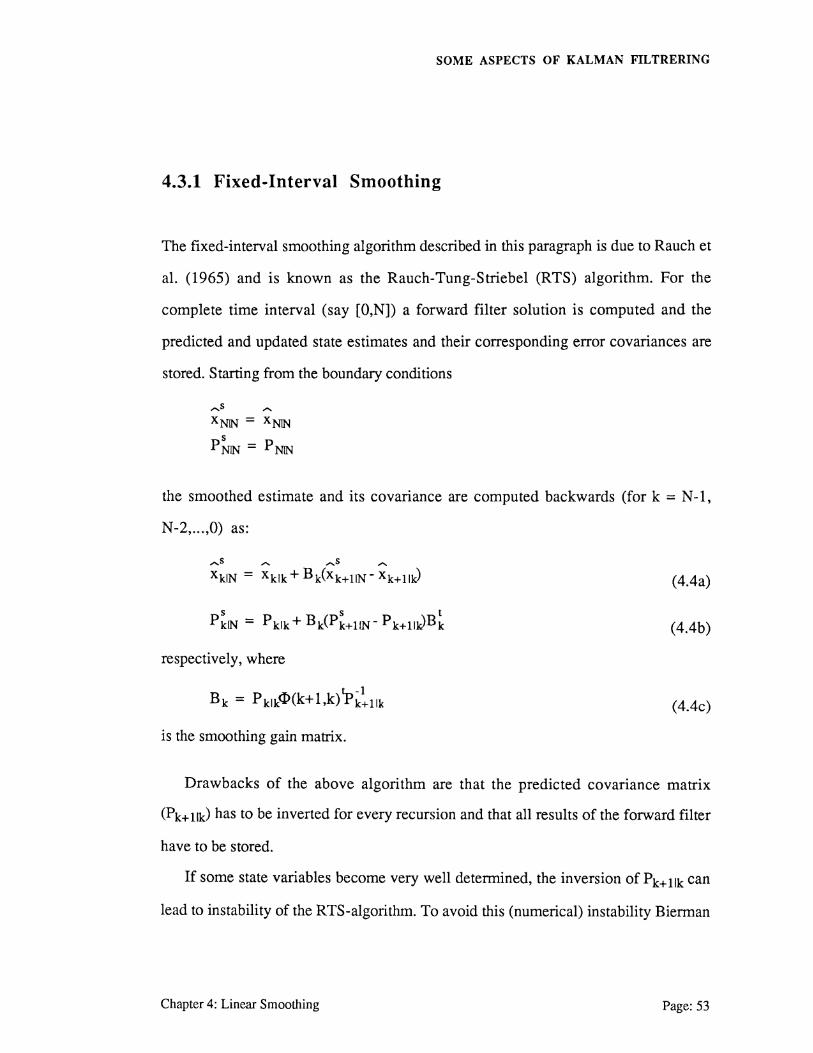
4.3.1 Fixed-Interval Smoothing
The fixed-interval smoothing algorithm described in this paragraph is due to Rauch et
al. (1965) and is known as the Rauch-Tung-Striebel (RTS) algorithm. For the
complete time interval (say [O,N]) a forward filter solution is computed and the
predicted and updated state estimates and their corresponding error covariances are
stored. Starting from the boundary conditions
XNIN = XNIN s
PNIN = PNIN
the smoothed estimate and its covariance are computed backwards (for k = N-1,
N-2, ... ,0) as:
"'s ,..., ,...s "' xkiN = xklk+ Bk(xk+liN- xk+ll0
respectively, where
t.-.. -1 Bk = Pklk<l>(k+ l,k) .t'k+llk
is the smoothing gain matrix.
(4.4a)
(4.4b)
(4.4c)
Drawbacks of the above algorithm are that the predicted covariance matrix
(Pk+llk) has to be inverted for every recursion and that all results of the forward filter
have to be stored.
If some state variables become very well determined, the inversion of Pk+llk can
lead to instability of the RTS-algorithm. To avoid this (numerical) instability Bierman
Chapter 4: Linear Smoothing Page: 53
SOME ASPECTS OF KALMAN FILTERING
[1973b] developed an alternative algorithm (Modified Bryson-Frazier smoother).
Gonthier [1984] found that if the smoother algorithm is implemented in double
precision arithmetic both algorithms lead to identical results and no numerical
problems are encountered.
In the forward-backward formulation of the smoother, as described in section 4.2,
the storage of intermediate results was not necessary. This, however, is only true if
merely one smoothed state estimate at time tk in the interval [O,N] is required. Besides,
the computational efficiency of the forward-backward formulation suffers from the
combined use of the covariance and inverse covariance filter mechanizations.
Because fixed-interval smoothers are mainly used in off-line processing storage
requirements are not critical. Off-line the implementation of the algorithm can be done
in double precision arithmetic, so that the RTS algorithm can be used.
4.3.2 Fixed-Point Smoothing
The fixed-point smoother as given in this paragraph is taken from Meditch [1969].
The fixed-point smoother uses the output of a standard forward running Kalman filter.
The initial values of the state and its error covariance are:
......_s
xklk = xklk s
pklk = pklk
Assume that the fixed-point estimate at a certain time tk is required. The optimal fixed-
point smoothed state estimate and its covariance are generated by the following system
of equations (fork fixed and j = k+ 1 ,k+2, ... ):
""'s "' ,..... .......... xklj = xklj-1 + CjCxjlj- xjlj-1) (4.5a)
Page 54 Chapter 4: Linear Smoothing
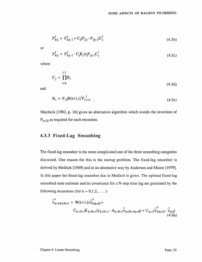
or
where
and
s s t pkl' = pkl' 1 + C·(P·~·- P·1· 1)C· J j- J J J J J- J
j-1
cj = TIBi i=k
SOME ASPECTS OF KALMAN FILTRERING
(4.5b)
(4.5c)
(4.5d)
(4.5e)
Maybeck [1982, p. 16] gives an alternative algorithm which avoids the inversion of
Pi+lli as required for each recursion.
4.3.3 Fixed-Lag Smoothing
The fixed-lag smoother is the most complicated one of the three smoothing categories
discussed. One reason for this is the startup problem. The fixed-lag smoother is
derived by Meditch [1969] and in an alternative way by Anderson and Moore [1979].
In this paper the fixed-lag smoother due to Meditch is given. The optimal fixed-lag
smoothed state estimate and its covariance for aN-step time lag are generated by the
following recursions (fork= 0,1,2, ... ):
~s ~s
xk+11k+N+1 = <I>(k+l,k)xklk+N+ .,....... ,.....s ""'
ck+N+lKk+N+l(Yk+N+l- Ak+N+lxk+N+llk+N) + u k+l(xklk+N- xkiiJ (4.6a)
Chapter 4: Linear Smoothing Page: 55
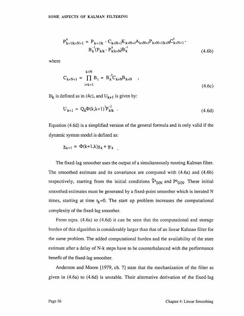
SOME ASPECTS OF KALMAN FILTERING
(4.6b)
where
(4.6c)
Bk is defined as in (4c), and Uk+l is given by:
t.,... ·1 u k+l = Qk<I>(k,k+ 1) t'klk . (4.6d)
Equation (4.6d) is a simplified version of the general formula and is only valid if the
dynamic system model is defined as:
The fixed-lag smoother uses the output of a simultaneously running Kalman filter.
The smoothed estimate and its covariance are computed with (4.6a) and (4.6b)
respectively, starting from the initial conditions ~sOIN and P8oiN· These initial
smoothed estimates must be generated by a fixed-point smoother which is iterated N
times, starting at time tk=O. The start up problem increases the computational
complexity of the fixed-lag smoother.
From eqns. (4.6a) to (4.6d) it can be seen that the computational and storage
burden of this algorithm is considerably larger than that of an linear Kalman filter for
the same problem. The added computational burden and the availability of the state
estimate after a delay of N-k steps have to be counterbalanced with the performance
benefit of the fixed-lag smoother.
Anderson and Moore [1979, ch. 7] state that the mechanization of the filter as
given in (4.6a) to (4.6d) is unstable. Their alternative derivation of the fixed-lag
Page 56 Chapter 4: Linear Smoothing
SOME ASPECTS OF KALMAN FILTRERING
smoother is quite long and will be not be repeated here. Furthermore Anderson and
Moore appear to be the only authors who seem to have noticed the inherent instability
of the presented algorithm. Even the more recent textbooks (e.g. Maybeck [1982],
Brown [1983]) give the fixed-lag smoother as derived by Meditch [1969].
To avoid the computational complexity of the fixed-lag smoother Brown [1983]
suggests the use of the RTS-algorithm if the lag is not too large. Using this approach
one filters forward to the current measurement and then sweeps back a fixed number
of steps with the RTS algorithm outlined in section 4.3.1. The start up problem can be
avoided by starting the backward sweep at time t = tlag· No smoothed estimates for
the first tlag instants are then available. Brown [1983, pp. 283-285] gives a solution
for the computation of these first estimates.
4.4. SMOOTHABILITY, GENERAL REMARKS, AND
APPLICATIONS
4.4.1 Smoothability
The defmition of smoothability is taken from Gelb [1974, p.163]: "A state is said to be
smoothable if an optimal smoother provides a state estimate superior to that obtained
when the final optimal filter estimate is extrapolated backwards in time". By defmition
only components of the state which are controllable with respect to the dynamic
system noise are smoothable. The concept of controllability is not discussed here; the
reader is referred to Maybeck [1979, Ch. 2].
Chapter 4: Linear Smoothing Page: 57
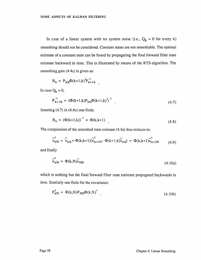
SOME ASPECTS OF KALMAN FILTERING
In case of a linear system with no system noise (i.e., Qk = 0 for every k)
smoothing should not be considered. Constant states are not smoothable. The optimal
estimate of a constant state can be found by propagating the final forward filter state
estimate backward in time. This is illustrated by means of the R TS-algorithm. The
smoothing gain (4.4c) is given as:
t....-1 Bk = Pklk<I>(k+l,k) l"'k+llk
In case (4 = 0,
Inserting (4.7) in (4.4c) one finds:
-1 Bk = (<I>(k+l,k)) = <I>(k,k+l)
The computation of the smoothed state estimate (4.4a) thus reduces to:
.-.s ........,s ......... ,....,.s
(4.7)
(4.8)
xkiN = xklk+ <I>(k,k+l)(xk+11N- <I>(k+l,k)xkiiJ = <I>(k,k+l)xk+11N (4.9)
andfmally
,....s ..... xkiN = <l>(k,N)xNIN (4.10a)
which is nothing but the final forward filter state estimate propagated backwards in
time. Similarly one finds for the covariance:
s t PkiN = <l>(k,N)P~(k,N) (4.10b)
Page 58 Chapter 4: Linear Smoothing

SOME ASPECTS OF KALMAN FILTRERING
4.4.2 General Remarks
In this chapter the algorithms for three classes of smoothing problems have been
presented. Although the algorithms may look very different, they also have a lot in
common.
• A (standard) forward running filter is at the basis of all smoothing algorithms. A smoothed estimate cannot be obtained without a simultaneously forward running filter.
• Unlike the filter algorithm (see Chapter 2) the computation of the smoothed state estimate (~\IN) does not require the computation of the corresponding smoothed covariance (P\IN)·
• For actual smoother implementations most programming effort is related to data management and storage problems.
4.4.3 Applications
For surveying applications mainly fixed-interval and fixed-lag smoothing are of
interest. Fixed-interval smoothing is usually performed off-line, because the (fixed)
interval of data can be quite long. Fixed-lag smoothing is the real-time oriented class
of smoothing problems, as the estimate of the state only lags for a certain lag tlag· For
on-line processing only fixed-lag smoothing is of interest. A fixed-lag smoother can
be implemented using the RTS-algorithm, as was suggested at the end of section
4.3.3.
Applications of smoothing techniques in surveying and hydrography are error
control for inertial systems [Gonthier, 1984], the postmission analysis of three
dimensional seismic campaigns at sea, and hydrographic surveys [Guenther and
Chapter 4: Linear Smoothing Page: 59

SOME ASPECTS OF KALMAN FILTERING
Thomas, 1987]. It seems, however, that for most kinematic or dynamic problems in
surveying filtering is deemed sufficient.
Smoothing may be a useful extension to filtering in kinematic positioning if now
and then no valid data are available due to, e.g., data outages or (rejected) outliers in
the data. As smoothing always implies forward filtering the optimal filtered estimate is
available, while smoothing may help bridge short data gaps.
Page60 Chapter 4: Linear Smoothing
SOME ASPECTS OF KALMAN FILTERING
5. PERFORMANCE ANALYSIS OF KALMAN FILTERS
-THE INNOVATIONS APPROACH-
5.1 INTRODUCTION
In kinematic positioning and navigation it is common to process data from different
sensors simultaneously in a so-called integrated navigation system to obtain a best
estimate of position. The algorithm implemented in these integrated navigation systems
is usually the Kalman filter. To obtain useful (positioning) results using an integrated
navigation system it is absolutely crucial that the performance of the underlying filter is
at an optimum. Therefore performance analysis of Kalman filters is of considerable
importance. Misspecifications in the dynamic and/or measurement model invalidate the
results of estimation. It is therefore essential to have ways to verify the validity of the
assumed mathematical model and to detect any misspecifications in the mathematical
model. An important role in the process of performance analysis is played by the so
called innovation sequence.
Methods for the detection of departures from optimality are all based on the
innovation sequence. Performance analysis of Kalman filters based on the innovation
sequence was introduced by Mehra and Peschon [1971]. The innovation sequence of
an optimal filter has precisely defined characteristics which can be compared with the
output of an actually implemented Kalman filter. The innovation process contains all
information to assess the optimality of filter operations. Furthermore the innovation
Chapter 5: Performance Analysis Page:61
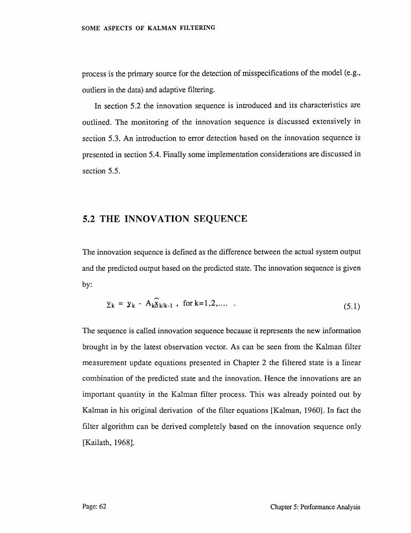
SOME ASPECTS OF KALMAN FILTERING
process is the primary source for the detection of misspecifications of the model (e.g.,
outliers in the data) and adaptive filtering.
In section 5.2 the innovation sequence is introduced and its characteristics are
outlined. The monitoring of the innovation sequence is discussed extensively in
section 5.3. An introduction to error detection based on the innovation sequence is
presented in section 5.4. Finally some implementation considerations are discussed in
section 5.5.
5.2 THE INNOVATION SEQUENCE
The innovation sequence is defined as the difference between the actual system output
and the predicted output based on the predicted state. The innovation sequence is given
by:
...... Yk = ~k - Ak~klk-1 , fork= 1 ,2,.... . (5.1)
The sequence is called innovation sequence because it represents the new information
brought in by the latest observation vector. As can be seen from the Kalman filter
measurement update equations presented in Chapter 2 the filtered state is a linear
combination of the predicted state and the innovation. Hence the innovations are an
important quantity in the Kalman filter process. This was already pointed out by
Kalman in his original derivation of the filter equations [Kalman, 1960]. In fact the
filter algorithm can be derived completely based on the innovation sequence only
[Kailath, 1968].
Page: 62 Chapter 5: Performance Analysis

SOME ASPECTS OF KALMAN FILTERING
For the objectives of this chapter the innovation sequence is considered to be the
output of the filter. For linear systems the output is Gaussian if the input is Gaussian
and thus the innovation sequence is considered to be Gaussian. Hence only the mean
and covariance of the innovation sequence have to be specified to describe the
statistical properties of the innovation sequence completely. Kailath [1968] has shown
that if the filter is optimal, the innovation sequence is a white noise sequence with zero
mean and known covariance (a sequence { x(n)} is called white (or purely random) if it
consists of a sequence of uncorrelated random variables). Thus:
where
(5.2)
is the covariance matrix of the innovation Y.k·
The covariance of the innovation has been encountered in the derivation of the
Kalman filter measurement update as well and thus it can be seen that the innovation
sequence is an integral part of the Kalman filter process.
Now the statistical properties of the innovation sequence have been described we
indicate how the innovations can be used for the performance analysis of the Kalman
filter. Since the properties of the innovation sequence are strictly defined if the filter is
optimal, the innovation sequence resulting from an actually implemented filter can be
monitored and compared to the faultless model description. Deviations from the
theoretical characteristics may be caused by mismodelling of the dynamic and/or
measurement model, failure of sensors, and outliers in the data. Mismodelling of any
Chapter 5: Performance Analysis Page:63

SOME ASPECTS OF KALMAN FILTERING
kind will make the innovation sequence depart from its theoretically defined nominal
values.
If the system is modelled perfectly, the innovations will be "small" and correspond
to random fluctuations in the output since all systematic trends are eliminated by the
model. If the model is misspecified, the innovations will be "large" and will display a
trend because the model no longer represents the physical system adequately. The
general performance of the filter can be monitored by analyzing the zero mean,
Gaussianness, given covariance, and whiteness of the innovation sequence.
Furthermore the innovation sequence is the sole source for outlier detection. Outlier
detection is also related to the wider field of failure detection, in which one tries to
detect abrupt changes, called failures, in dynamical systems. The general theory of
failure detection falls outside the scope of this paper. A survey of this topic is given by
Willsky [1976]. Finally the innovation sequence offers a possible approach to adaptive
filtering. Adaptive filtering techniques based on the innovation sequence are reviewed
by Chin [1979]. The innovations approach thus facilitates an array of very useful
Kalman filter related techniques.
5.3 MONITORING THE INNOVATION SEQUENCE
In this section we will focus our attention on the performance analysis of Kalman
filters based on the approach of Mehra and Peschon [1971]. In their approach the
innovation sequence is analyzed in the time domain and is used to assess the general
performance of the filter. To facilitate performance analysis in both on-line and off-line
environments the approach in the time domain is pursued throughout.
Page: 64 Chapter 5: Performance Analysis
SOME ASPECTS OF KALMAN FILTERING
In monitoring the innovation sequence the assumption is that the filter operates at
an optimum, i.e., the innovation sequence is zero mean, Gaussian, white, and of
known covariance. This constitutes our so-called null hypothesis. The alternative
hypothesis is that the null hypothesis is false. In the approach described in this section
all characteristics of the innovation sequence are tested separately. The null hypothesis
will not be tested in a large, all encompassing, test. In this section only tests for
departures from the null hypothesis are presented. No methods for system diagnosis
(i.e., determining the cause of of a detected departure) are presented.
Before the actual monitoring techniques are discussed a general philosophy of data
analysis, that is basically adhered to in this section, is outlined. Bendat and Piersol
[ 1986] describe a general strategy for data acquisition and data processing. Once the
data - in our case the innovations - have been obtained two actions are
distinguished: data qualification and data analysis. Data qualification should precede
data analysis, but in practice data qualification and data analysis are usually performed
at the same time.
Data qualification encompasses the investigation of the basic characteristics of the
data, namely: stationarity, presence of periodicities, and normality. A sequence is
called stationary if its statistical properties do not change in time. Stationarity of a
sequence can often be derived from the properties of the underlying model generating
the random data. In case of an optimal linear Kalman filter one expects a stationary
innovation sequence. Nonstationarity in a stochastic sequence can, for instance, be
revealed as a trend in the mean value of the data. Periodicity of the data is not
investigated explicitely. Some inferences regarding periodicities can be made from the
estimated autocorrelation function, to be discussed shortly.
Chapter 5: Performance Analysis Page:65
SOME ASPECTS OF KALMAN FILTERING
Whiteness is the most important property of the innovation sequence. If whiteness
of the innovation sequence is not established, data analysis cannot be performed
properly. To test if the sequence of innovations is independent Bendat and Piersol
[1986] introduce two non-parametric tests, namely, the run test and the reverse
arrangements test. Non-parametric means that no assumptions concerning the
probability distribution of the data being evaluated are made.
Although it has been stated several times that the innovation sequence is Gaussian
if the observations are distributed normally, normality has to be verified. The
equivalence of the probability density function of the innovations to the normal density
function is tested by means of the (Chi-square) goodness-of-fit test, once more a non
parametric test [Bendat and Piersol, 1986].
Independence can also be tested with tests based on the autocorrelation function.
The autocorrelation function describes the correlation between data for various time
lags and renders some more information than the run test and reverse arrangements
test. By means of the autocorrelation function one may, for example, be able to reveal
periodicities in the data.
Although it would seem logical to start with a test of the mean of the innovation
sequence, we will defer the tests of mean to a later stage because they are dependent on
the estimate of the covariance, which in its turn is based on the assumption of
whiteness. We will see that to perform the analysis of whiteness, the sample mean of
the innovation sequence still has to be computed first, only its analysis is deferred to a
later stage.
In the following time series and statistical techniques are used extensively. An
overview of these topics can be found in Priestley [1981] and Morrison [1976]
Page: 66 Chapter 5: Performance Analysis

SOME ASPECTS OF KALMAN FILTERING
respectively. To ease the derivations normalized innovations are considered in the rest
of this section:
(5.3)
so that
t
E{ykyl} = 10kt · (5.4)
In the following N denotes sample size (the number of samples used to analyse the
innovation sequence).
The autocorrelation function Pk of a stationary (normalized innovation) sequence
for a lag k is defined as:
t Pk = E {(yi- v )(yi+k- v)}, for k=0,±1,±2, .... (5.5)
where v denotes the expected value of Yi (i.e., v = E {.Y.il ).
Assuming that the innovation sequence is ergodic (a sequence is called ergodic if
its ensemble averages (eqn. 5.5) correspond with its time averages (eqn. 5.6)) the
autocorrelation function can be estimated as:
k = 0,±1,±2, ... , ±(N-1)
(5.6)
...... where vis the sample mean
(5.7)
Under the null hypothesis the autocorrelation functions for different lags k are
asymptotically independent and are normally distributed with zero mean and
Chapter 5: Performance Analysis Page:67
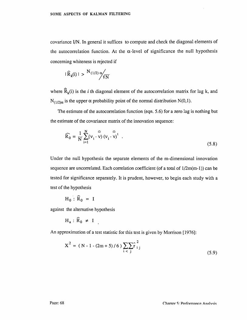
SOME ASPECTS OF KALMAN FILTERING
covariance 1/N. In general it suffices to compute and check the diagonal elements of
the autocorrelation function. At the a-level of significance the null hypothesis
concerning whiteness is rejected if
A
where Rk(i) is the i th diagonal element of the autocorrelation matrix for lag k, and
N(1/2)a is the upper a. probability point of the normal distribution N(O,l).
The estimate of the autocorrelation function (eqn. 5.6) for a zero lag is nothing but
the estimate of the covariance matrix of the innovation sequence:
(5.8)
Under the null hypothesis the separate elements of the m-dimensional innovation
sequence are uncorrelated. Each correlation coefficient (of a total of l/2m(m-1)) can be
tested for significance separately. It is prudent, however, to begin each study with a
test of the hypothesis
. "" H 0 : R0 = I
against the alternative hypothesis
An approximation of a test statistic for this test is given by Morrison [1976]:
Page:68
X 2 = ( N- 1- (2m+ 5) I 6) LL~ ~j i < j (5.9)
C.h:mter 'i~ Perform~n~e An~lv<;:i<;:

SOME ASPECTS OF KALMAN FILTERING
A
where rij are the elements of matrix R0. The statistic X2 has a Chi-squared distribution
with l/2m(m-1) degrees of freedom. The null hypothesis is rejected at the a.-level of
significance whenever
2 2 X > Xa; l/2m(m-1)
where :x2a;l/2m(m-l) is the upper a. probability point of the Chi-squared distribution
x21/2m(m-1) with 1/2m(m-1) degrees of freedom.
The correlation coefficients can also be tested separately. Subject to some
conditions [Bendat and Piersol, 1986] the quantity
i < j (5.10)
is distributed approximately normal under the null hypothesis with zero mean and
variance
~-3.
The null hypothesis concerning a single correlation coefficient between elements of the
innovation sequence is rejected at the a.-level of significance if
I w . ·I > N (l/2)a/ lJ /{N-3 .
If it is established that the innovation sequenece is white (i.e., correlations in time
are negligible) the covariance matrix (which under the null hypothesis corresponds to
the correlation matrix for a zero lag) and the mean can be tested. Both tests assume that
the innovation sequence is white.
Morrison [1976] shows that under the null hypothesis the covariance matrix times
"' N (i.e. N*Ro) has a Wishart distribution. Mehra and Peschon [1971] state that the
Chapter 5: Performance Analysis Page:69

SOME ASPECTS OF KALMAN FILTERING
A trace of Ro has a Chi-squared distribution with (n-1)m degrees of freedom. Using the
trace of the sample covariance matrix it can thus be tested easily if the covariance
matrix is equal to the identity matrix.
Under the null hypothesis the innovation sequence is zero mean and the mean
(eqn. 5.7) is normally distributed and has a covariance of 1/N. At the a-level of
significance the null hypothesis concerning the zero mean is rejected whenever
I vi I > N 112a, i=1, ... ,m .
As is indicated in Mehra and Pesch on [1971] this test suffers from the fact that the
covariance of the innovation sequence is assumed to be known. They propose to use
'f2-statistic instead:
~ t 1~ 2 ...... -T =Nv R0 v (5.11)
The derivation of this statistic can be found in Morrison [1976]. Under the null
hypothesis the quantity is distributed according to the F-distribution with m and N-m
degrees of freedom. The null hypothesis concerning the mean is rejected at the a-level
of significance if
T2 > m(N -1) F N _ m a; m,N-m
In this section a general methodology for the analysis of (normalized) innovation
sequences has been presented. Departures from zero mean, normality, whiteness, and
a known covariance can be detected by the methods described herein. The described
techniques, however, pertain to the innovation sequence in general. More specific
alternative hypotheses could be formulated if one has some idea of the causes leading
to the departures from nominal values (e.g., sensor failures, outliers in the data, etc.).
Page:70 Chapter 5: Perfonnance Analysis

SOME ASPECTS OF KALMAN FILTERING
As part of the innovation sequence monitoring and analysis some extra model
parameters can be estimated. One can try, for instance, to derive a possible model that
accounts for departures from whiteness. The reader is referred to Priestley [1981] for
details about the estimation of additional parameters.
5.4 ERROR DETECTION
Now that several techniques to monitor the general filter performance using the
innovation sequence have been discussed, another important application of the
innovation sequence can be introduced. We restrict ourselves to a specific application
of the monitoring of the innovation sequence. The innovation process can be used to
detect outliers in the observations.
In section 5.2 we defined the innovation sequence as the sequence that contains all
new information brought in by the latest observation. An outlier in the observations is
certainly new information as the filter model cannot anticipate possible outliers.
Therefore the innovation sequence is at the base of all outlier detection algorithms.
Outliers in the data affect the property of zero mean of the innovation sequence. In
statistics and adjustment theory various tests have been developed which deal with
such phenomena. Misspecifications of the model at a certain time can be detected by a
so-called overall model test. A misspecification detected by such an overall model
test can be diagnosed further by a so-called slippage test if the misspecification
affects the property of zero mean of the random variable. The application of overall
model and slippage tests to Kalman filter performance analysis is discussed in
Teunissen and Salzmann [1988]. The use of these tests in a more general setting in
Chapter 5: Performance Analysis Page:71
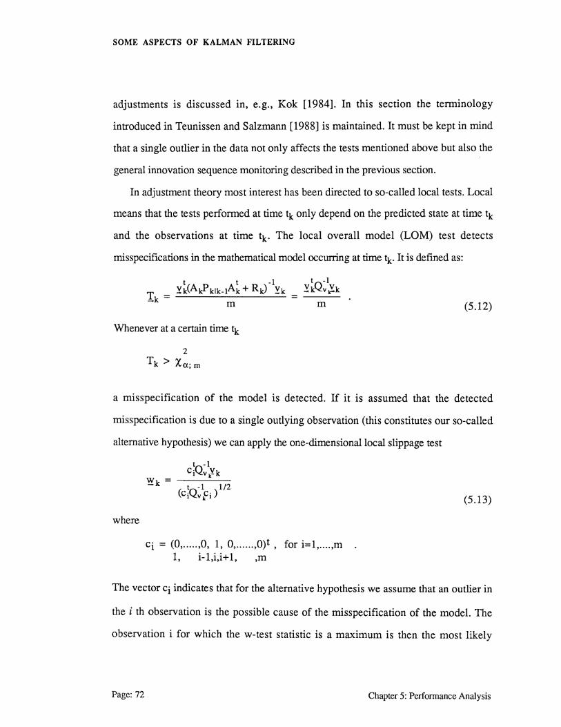
SOME ASPECTS OF KALMAN FILTERING
adjustments is discussed in, e.g., Kok [1984]. In this section the terminology
introduced in Teunissen and Salzmann [1988] is maintained. It must be kept in mind
that a single outlier in the data not only affects the tests mentioned above but also the
general innovation sequence monitoring described in the previous section.
In adjustment theory most interest has been directed to so-called local tests. Local
means that the tests performed at time tk only depend on the predicted state at time tk
and the observations at time tk. The local overall model (LOM) test detects
misspecifications in the mathematical model occurring at time tk. It is defined as:
(5.12)
Whenever at a certain time tk
a misspecification of the model is detected. If it is assumed that the detected
misspecification is due to a single outlying observation (this constitutes our so-called
alternative hypothesis) we can apply the one-dimensional local slippage test
~k = (5.13)
where
Ci = (0, ..... ,0, 1, O, ...... ,O)t , for i=1, .... ,m . 1, i-l,i,i+l, ,m
The vector Ci indicates that for the alternative hypothesis we assume that an outlier in
the i th observation is the possible cause of the misspecification of the model. The
observation i for which the w-test statistic is a maximum is then the most likely
Page:72 Chapter 5: Performance Analysis

SOME ASPECTS OF KALMAN FILTERING
outlying observation. In general other alternative hypotheses may be specified and this
will affect the form of the c-vector.
Equations (5.12) and (5.13) show that the test statistics are functions of the
innovations. The above tests, frequently applied in adjustments, have the advantage
that they can be executed in real time. Corrective action is thus also possible in real
time.
To apply testing methods for the detection of outliers the null hypothesis and the
alternative hypothesis have to be defined quite precisely. The mere introduction of
system noise in the filter model indicates that in general the knowledge of the
underlying model for dynamic systems is not as perfect as in problems usually
considered in surveying. Furthermore it is expected that in dynamic environments the
measurement sensors are more prone to failures of any kind. Apart from the fact that
the modelling of dynamic systems may not be as sophisticated as the models used in
classical adjustment problems in surveying, often also the redundancy for a single
Kalman filter measurement update can be quite low. Therefore a more cautious
approach is usually followed for error detection in dynamic systems as the local tests
may not be able to detect global unmodelled trends.
In Willsky [1976] the following test statistic is defined:
k L t t -1 v·(A·P·1• 1A + R-) v· -1 1 11- 1 1 -1
i=k-M+l (5.14)
where M denotes the delay one is willing to accept in detecting a model
misspecification. In practice a small delay M may be acceptable, though no real-time
corrective action can be taken anymore. It can be seen that (5.14) actually represents
nothing but a sum of the local overall model test statistics introduced earlier. The test
Chapter 5: Performance Analysis Page: 73
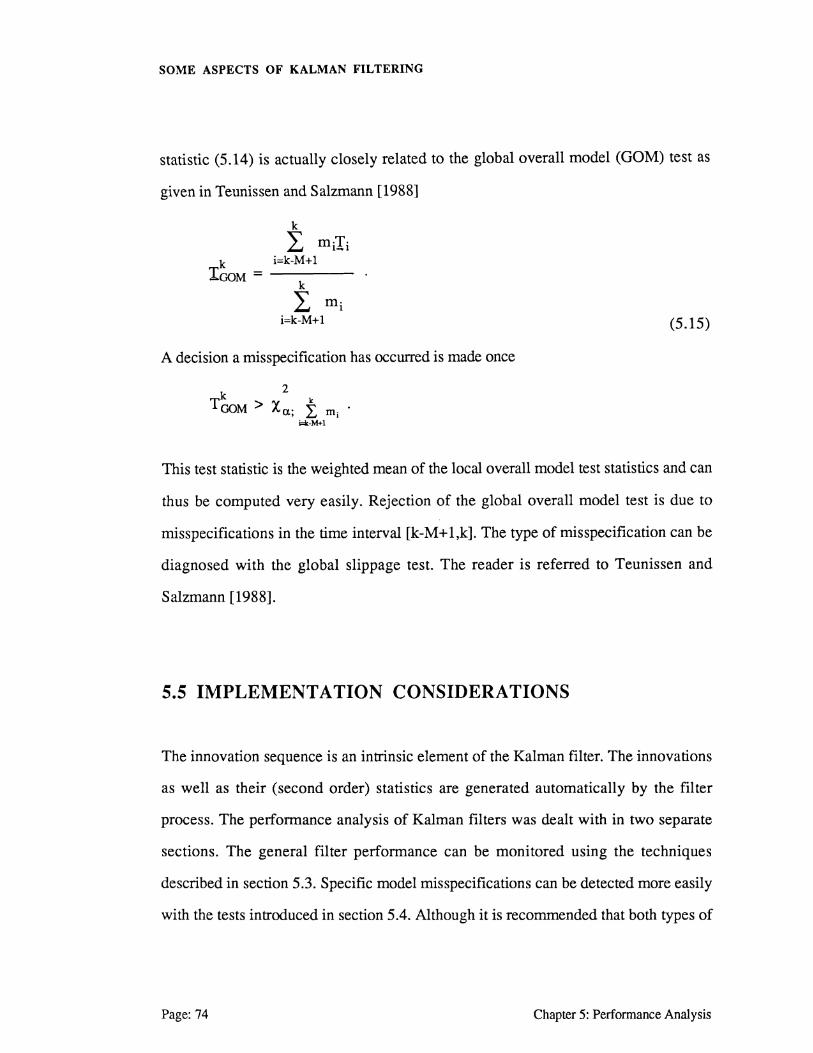
SOME ASPECTS OF KALMAN FILTERING
statistic (5.14) is actually closely related to the global overall model (GOM) test as
given in Teunissen and Salzmann [1988]
k ~ m·T· £..J 1-1
i=k-M+l k IooM = ---
k
L mi i=k-M+l
A decision a misspecification has occurred is made once
k 2 TooM > Xa.; f. m;
i=lr.-M+1
(5.15)
This test statistic is the weighted mean of the local overall model test statistics and can
thus be computed very easily. Rejection of the global overall model test is due to
misspecifications in the time interval [k-M+ 1,k]. The type of misspecification can be
diagnosed with the global slippage test. The reader is referred to Teunissen and
Salzmann [1988].
5.5 IMPLEMENTATION CONSIDERATIONS
The innovation sequence is an intrinsic element of the Kalman filter. The innovations
as well as their (second order) statistics are generated automatically by the filter
process. The performance analysis of Kalman filters was dealt with in two separate
sections. The general filter performance can be monitored using the techniques
described in section 5.3. Specific model misspecifications can be detected more easily
with the tests introduced in section 5.4. Although it is recommended that both types of
Page:74 Chapter 5: Performance Analysis
SOME ASPECTS OF KALMAN FILTERING
performance analysis techniques should be implemented some remarks concerning
their implementation are made.
The general filter performance analysis is extremely useful in the design and
implementation stage of a Kalman ftlter. If the performance analysis can be performed
off-line (which will usually be the case in the design stage), the full range of analysis
techniques described in section 5.3 can be applied. It is felt, however, that this
performance analysis can be executed in an on-line environment as well. The extent of
the on-line performance analysis depends primarily on the computer power available.
The number of samples used to analyse the innovation sequence (i.e., N) should
neither be chosen too small or too large. A large value of N (e.g., N>200) requires
considerable computing time, whilst a too small N (e.g., N <50) does not enable a
proper time series analysis. Depending on the computer facilities available a happy
medium has to be found for on-line applications. The analysis discussed in section 5.3
requires computations every Nth cycle of the Kalman filter. For on-line environments
it is suggested that the general performance analysis be used as an alarm system. If the
null hypothesis (i.e., the Kalman filter operates at an optimum and thus the innovation
process has strictly defined statistical properties) is (constantly) rejected, the user
should be informed. If sufficient computer power is available, it can even be attempted
to estimate extra model parameters that account for the possible departures from the
nominal characteristics of the innovation sequence. If no additional parameters are
estimated, the monitoring of the innovation sequence constitutes a fault detection
technique. A diagnosis of what causes the ftlter to depart from its optimal properties is
generally not performed.
To detect misspecifications in the model on a real time or nearly real-time basis
specific tests were introduced in section 5.4. It was shown that especially the local
Chapter 5: Performance Analysis Page:75

SOME ASPECTS OF KALMAN FILTERING
tests can be implemented very easily. As the local redundancy in Kalman filter
measurement updates is sometimes quite low and the dynamic model may not be very
well defined it can be advantageous to implement the global overall model test and the
global slippage test if a small delay in the error detection is acceptable. For the global
tests the delay (i.e., M) should not be chosen too large. Firstly, a large M will hamper
taking corrective action if a misspecification has been detected. Secondly, a large M
may decrease the probability of correct detection of a model misspecification because
averaging over a large number of innovations may smooth out the effect of a model
misspecification. As a diagnostic tool (particularly if the model misspecifications are
caused by outliers in the data) the tests described in section 5.4 are very powerful and
supplement the general analysis discussed in section 5.3.
As far as outliers in the data or sensor failures are not the cause for departures from
the nominal characteristics of the innovation sequence, misspecifacations of the system
and measurement noise are usually at the basis of these departures. This brings us into
the realm of adaptive filtering which is outside the scope of this chapter. The interested
reader is referred to Chin [1979].
Page:76 Chapter 5: Performance Analysis
SOME ASPECTS OF KALMAN FILTERING
6. SUMMARY
The use of Kalman filters in kinematic positioning is well established. In this report
several aspects of Kalman filtering are reviewed that pertain to kinematic positioning
problems. Actual applications of Kalman filtering techniques to specific kinematic
positioning problems are not considered.
Linear Kalman Filter
A general discrete time dynamic and measurement models are introduced and the
linear Kalman filter for this model is subsequently derived using a least-squares
approach. It is indicated how continuous time models can be transformed to equivalent
discrete time models. Some attention is paid to possible nonlinearities of the model.
For applications in hydrography and surveying the iterated extended Kalman filter is
probably the most frequently applied filter algorithm.
Computational Considerations
For actual implementations of Kalman filters various filter mechanizations can be
used. If frequent estimates of the state and its covariance are required (as is the case in
kinematic positioning) the so-called covariance filter mechanizations are to be
preferred. In these mechanizations the covariance of the system state is propagated in
time. It is found that if double precision arithmetic is used in the filter computations no
numerical difficulties arise for any filter mechanization and thus the most efficient
mechanization can be implemented. If computations have to performed in single
Chapter 6: Summary Page:77

SOME ASPECTS OF KALMAN FILTERING
precision arithmetic or the reduction of the computational burden is of the utmost
importance, the U-D covariance factorization filter can be considered for
implementation. This mechanization is closely related to the square root covariance
filters. For every application considerable computational savings can be achieved if the
problem structure is taken into account.
Linear Smoothing
The number of applications of smoothing techniques is rather limited because of
the delay inherent in the smoothing algorithm. In situations where off-line
computations are feasible, however, smoothing techniques can greatly enhance the
position estimates in a postmission approach. Conceptually the smoothing problem can
be decomposed into two filtering problems. The smoothed estimate can be obtained
from a combination of the two filtered estimates. The classes of fixed-interval, fixed
point, and fixed-lag smoothing are discussed. For kinematic positioning problems
fixed-interval smoothing seems most appropriate for a postmission approach. If a
small delay in obtaining the state estimate is acceptable, a fixed-lag smoother can be
considered for "real-time" applications.
Performance Analysis
If a Kalman filter operates at an optimum, the innovation sequence generated by
the filter has some very well defined statistical properties. Any misspecification in the
filter model will cause departures from these optimal characteristics. Therefore the
innovation sequence of an actually implemented Kalman ftlter is the primary source for
the analysis of the performance of the filter. A general filter performance analysis
methodology is discussed which basically functions as an alarm system. General and
Page:78 Chapter 6: Summary

SOME ASPECTS OF KALMAN FILTERING
specific misspecifications in the model, in particular outliers in the observations, can
be detected and diagnosed with the overall model test and the slippage tests
respectively. These test statistics are also functions of the innovations.
Chapter 6: Summary Page:79

SOME ASPECTS OF KALMAN FILTERING
Page: 80 Chapter 6: Summary

SOME ASPECTS OF KALMAN FILTERING
BIBLIOGRAPHY
Anderson, B.D.O.and J.B. Moore (1979). Optimal Filtering. Prentice-Hall, Englewood-Cliffs, NJ.
Ayers, H.B. (1985). Least-squares radio positioning in the offshore Environment. UCSE Report #20012, Division of Surveying Engineering, University of Calgary.
Bendat, J.S. and A.G. Piersol (1986). Random Data: Analysis and Measurement Procedures. 2nd ed.,Wiley-Interscience, New York.
Bierman. G.J. (1973a). A comparison of discrete linear filtering algorithms. IEEETrans. on Aerospace and Electronic Systems, Vol. IEEE-AES 9(1), pp. 28-37.
Bierman, G.J. (1973b). Fixed interval smoothing with discrete measurements. Int. Journal of Control, Vol. 18(1), pp. 65-75.
Bierman, G.J. (1977). Factorization Methods for Discrete Sequential Estimation. Academic Press, New York.
Box, G.E.P and G.M. Jenkins, (1970). Time Series Analysis Forecasting and Control. Holden-Day, San Francisco.
Brown, R.G. (1983). Introduction to Random Signal Analysis and Kalman Filtering. Wiley, New York.
Chin, L. (1979). Advances in adaptive filtering. In: Control and Dynamic Systems, Vol. 15, Ed. C.T. Leondes, Academic Press, New York.
Chin, L. (1983). Advances in computational efficiencies of linear filtering. In: Control and Dynamic Systems, Vol. 19, Ed. C.T. Leondes, Academic Press, New York.
Gelb, A. (ed.) (1974). Applied Optimal Estimation. MIT-Press, Cambridge, Ma.
Gonthier, M. (1984). Smoothing procedures for inertial survey systems of local level type. UCSE Report #20008, Division of Surveying Engineering, University of Calgary.
Guenther, G.C. and W.L. Thomas (1987). Optimum utilization of positioning data in SDS III. International Hydrographic Review, Vol 64(1), pp. 35-58.
Gylys, V.B. (1983). Design of real-time estimation algortihms for implementation in microprocessor and distributed processor systems. In: Control and Dynamic Systems, Voll9, Ed.C.T. Leondes, Academic, New York.
Bibliography Page:81

SOME ASPECTS OF KALMAN FILTERING
Hasenack, E. (1986). Precision and reliability of a Kalman filter (in Dutch). Thesis, Department of Geodesy, Delft University of Technology.
Houtenbos, A.P.E.M. (1982). Prediction, filtering, and smoothing of offshore navigation data. The Hydrographic Journal, No. 25, pp. 5-16.
Jazwinski, A.H. (1970). Stochastic Processes and Filtering Theory. Academic Press, New York.
Jenkins, G.M. and D.G. Watts (1968). Spectral Analysis and its Applications. Holden-Day, San Francisco.
Kailath, T. (1968). An innovations approach to least-squares estimation Part I: Linear filtering in additive white noise. IEEE-Trans. on Automatic Control, Vol. IEEEAC 13(6), pp.646-655.
Kailath, T. and P. Frost (1968). An innovations approach to least-squares estimation Part II: Linear smoothing in additive white noise. IEEE-Trans. on Automatic Control, Vol. IEEE-AC 13(6), pp. 655-660.
Kalman, R.E. (1960). A new approach to linear filtering and prediction problems. ASME Journal of Basic Engineering, Vol. 82, pp. 34-45.
Kaminski, P.G., A.E. Bryson, and S.F. Schmidt (1971). Discrete square root filtering: A survey of current techniques. IEEE Trans. on Automatic Control, Vol. IEEE-AC 16(6), pp. 727-736.
Koch, K.R. (1982). Kalman filter and optimal smoothing derived by the regression model, Manuscripta Geodaetica, Vol. 7(2), pp. 133-144.
Kok, J.J. (1984). On Datasnooping and Multiple Outlier Testing. NOAA Technical Report NOS NGS 30, U.S. Department of Commerce, Rockville, Md.
Krakiwsky, E. (1975). A synthesis ofrecent advances in the method of least squares. Department of Surveying Engineering, Lecture Notes #24,University of New Brunswick.
LeMay, J.L. (ed.) (1984). Kalman Filtering (2 volumes). Lecture notes of a five day short course, Aug. 27-31, University of California at Los Angeles.
Maybeck, P.S. (1979). Stochastic Models, Estimation, and Control. Vol. 1, Academic Press, New York.
Maybeck, P.S. (1982). Stochastic Models, Estimation, and Control. Vol. 2, Academic Press, New York.
Meditch, J.S. (1969). Stochastic Optimal Linear Estimation and Control. McGrawHill, New York.
Meditch, J.S. (1973). A survey of data smoothing for linear and nonlinear dynamic systems. Automatica, Vol. 9, pp. 151-162.
Page:82 Bibliography
SOME ASPECTS OF KALMAN FILTERING
Mehra, R.K., and J. Peschon (1971). An innovations approach to fault detection and diagnosis in dynamic systems. Automatica, Vol. 7, pp. 637-640.
Morrison, D.F. (1976). Multivariate Statistical Methods. 2nd ed, McGraw-Hill, New York.
Priestley, M.B. (1981). Spectral Analysis and Time Series. Academic Press, London.
Rauch, H.E., F. Tung, and C.T. Striebel. (1965). Maximum likelihood estimates of linear dynamic systems. AIAA Journal, Vol8(3), pp. 1445-1450.
Salzmann, M.A. (1988). The impact of system integration on position estimation- two case studies. Department of Surveying Engineering, Technical Memorandum, University of New Brunswick.
Teunissen, P.J.G. and M.A. Salzmann (1988). Performance analysis of Kalman filters. Paper presented at HYDR088, Amsterdam, 15-17 November.
Thornton, C.L. and G.J. Bierman (1980). UDUt covariance factorization for Kalman Filtering. In: Control and Dynamic Systems, Vol. 16, Ed. C.T. Leondes, Academic, New York.
Upadhyay, T.N. and J.N. Damoulakis (1980). Sequential piecewise recursive filter for GPS low dynamics navigation. IEEE-Trans. on Aerospace and Electronic Systems. Vol. IEEE-AES 16(4), pp. 481-491.
Verhaegen, M. and P. van Dooren (1986). Numerical aspects of different Kalman filter implementations. IEEE Trans. on Automatic Control, Vol. IEEE-AC 31(10), pp. 907-917.
Willsky, A.S., (1976). A survey of design methods for failure detection in dynamic systems. Automatica, Vol12, pp.601-611.
Bibliography Page:83

SOME ASPECTS OF KALMAN FILTERING
Page: 84 Bibliography
SOME ASPECTS OF KALMAN FILTERING
APPENDIX I
U-D COVARIANCE FACTORIZATION FILTER MECHANIZATION
In this appendix (pseudo) FOR1RAN mechanizations of the basic computational parts
of the U-D filter are given. The mechanizations are kept as simple as possible in order
to provide a more detailed insight than is provided by the general algorithms. The
mechanizations are derived from the algorithms as given in Maybeck [1979, pp. 392-
397]. These algorithms are not necessarily the most efficient ones computationally.
Special (and probably faster) mechanizations can be found in Bierman [1977] and
Thornton and Bierman [ 1980] (in the latter publication some printing errors are present
· in the provided FOR1RAN mechanizations).
For actual implementation the programmer can exploit the unitary upper triangular
characteristic of the U-factor. The elements of the D-factor can be stored on the
diagonal of U. Storage requirements can be reduced further by storing the matrices
vector-wise. In these cases some bookkeeping logic has to be added.
In the mechanizations n, s, and m denote the dimension of the state vector, the
dimension of the system noise vector, and the dimension of the observation process
respectively.
Appendix! Page: 85
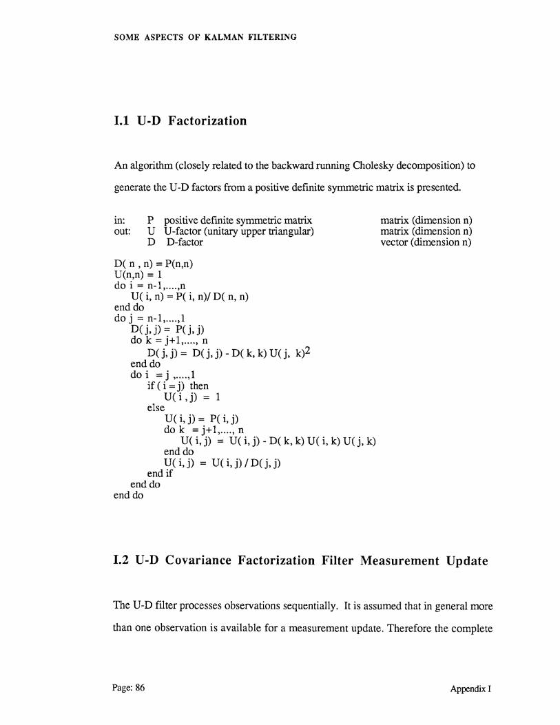
SOME ASPECTS OF KALMAN FILTERING
1.1 U -D Factorization
An algorithm (closely related to the backward running Cholesky decomposition) to
generate the U-D factors from a positive definite symmetric matrix is presented.
m: P positive definite symmetric matrix out: U U-factor (unitary upper triangular)
D D-factor
D( n , n) = P(n,n) U(n,n) = 1 do i = n-1, .... ,n
U( i, n) = P( i, n)/ D( n, n) end do do j = n-1, .... ,1
D(j,j) = P(j,j) do k = j+1, .... , n
D(j,j)= D(j,j)-D(k,k)U(j, k)2 end do do i = j , .... ,1
if ( i = j) then U(i,j) = 1
else U( i, j) = P( i, j) do k = j+1, .... , n
U( i, j) = U( i, j)- D( k, k) U( i, k) U( j, k) end do U(i,j) = U(i,j)/D(j,j)
end if end do
end do
matrix (dimension n) matrix (dimension n) vector (dimension n)
1.2 U-D Covariance Factorization Filter Measurement Update
The U-D filter processes observations sequentially. It is assumed that in general more
than one observation is available for a measurement update. Therefore the complete
Page: 86 Appendix I
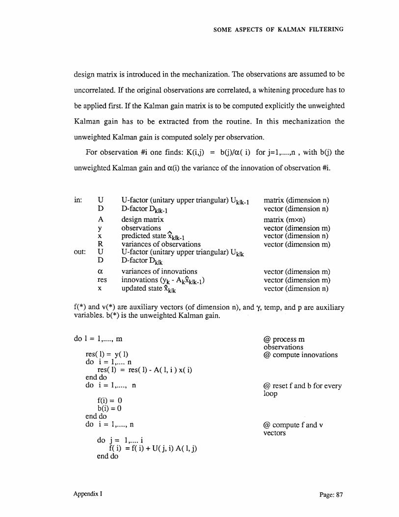
SOME ASPECTS OF KALMAN FILTERING
design matrix is introduced in the mechanization. The observations are assumed to be
uncorrelated. If the original observations are correlated, a whitening procedure has to
be applied first. If the Kalman gain matrix is to be computed explicitly the unweighted
Kalman gain has to be extracted from the routine. In this mechanization the
unweighted Kalman gain is computed solely per observation.
For observation #i one finds: K(i,j) = b(j)/a( i) for j=1, .... ,n , with b(j) the
unweighted Kalman gain and a(i) the variance of the innovation of observation #i.
in: u D
A y X
R out: U
D
a res X
U-factor (unitary upper triangular) Uklk-1 D-factor ~lk-1 design matrix observations predicted state ~klk-1 variances of observations U-factor (unitary upper triangular) Uklk D-factor ~lk
variances of innovations innovations (Yk - Akxklk-1) updated state ~klk
matrix (dimension n) vector (dimension n)
matrix (mxn) vector (dimension m) vector (dimension n) vector (dimension m)
vector (dimension m) vector (dimension m) vector (dimension n)
f(*) and v(*) are auxiliary vectors (of dimension n), andy, temp, and pare auxiliary variables. b(*) is the unweighted Kalman gain.
do 1 = 1, .... , m
res( 1) = y( 1) do i = 1, .... n
res( 1) = res( 1) - A( 1, i ) x( i) end do do i = 1, .... , n
f(i) = 0 b(i) = 0
end do do i = 1, .... , n
do j = 1, .... i f( i) = f( i) + U(j, i) A(l,j)
end do
Appendix!
@process m observations @ compute innovations
@ reset f arid b for every loop
@ compute f and v vectors
Page:87
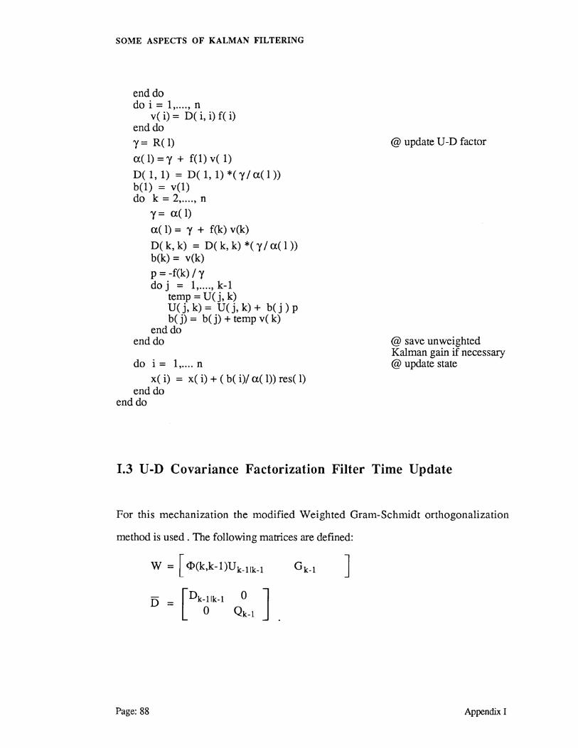
SOME ASPECTS OF KALMAN FILTERING
end do do i = 1, .... , n
v( i) = D( i, i) f( i) end do
y= R(l)
a( 1) = y + f(1) v( 1)
D( 1, 1) = D( 1, 1) *(y/a(l )) b(1) = v(1) do k = 2, .... , n
y= a( 1)
a( 1) = y + f(k) v(k)
D( k, k) = D( k, k) *( y I a(l )) b(k) = v(k)
p=-f(k)/y do j = 1, .... , k-1
temp= U(j, k) U(j, k) = U(j, k) + b(j) p b( j) = b( j) + temp v( k)
end do end do
do i = 1, .... n x( i) = x( i) + ( b( i)/a( 1)) res( 1)
end do end do
@ update U-D factor
@ save unweighted Ka1man gain if necessary @ update state
1.3 U -D Covariance Factorization Filter Time Update
For this mechanization the modified Weighted Gram-Schmidt orthogonalization
method is used . The following matrices are defined:
W = [ <l>(k,k-1)Uk_11k_ 1 J D = [Dk-11k-1 0 J
0 Qk-1
Page: 88 Appendix I

SOME ASPECTS OF KALMAN FILTERING
In actual implementations the matrices Wand i5 have not to be used explicitely. The
matrix W is destroyed completely during the update. The system noise variances
(stored in Qc_1) remain unchanged.
in: W matrix (nx(n+s)) U U-factor (unitary upper triangular) Uk-11k-1 matrix (dimension n) D D-factor and diagonal part system noise vector (dimension n+s)
out: U updated U-factor (unitary upper triangular) Uklk-1 D updated D-factor Dklk:-1
c(*) and d(*) are auxiliary vectors of dimension (n+s).
do k = n, .... ,1 do j = 1, .. .:.:1 n+s
c(j) = D(j,j) W( k,j) end do D( k, k) = 0 do j = 1, .... , n+s
D( k, k) = D( k, k) + W( k, j) c(j) end do do j = 1, .... , n+s
d( j) = c( j) I D( k, k) end do do j = 1, .... , k-1
U(j,k)=O do j = 1, .... , n+s
U(j, k) = U(j, k) + W(j, i) d( i) end do do i = 1, .... , n+s
W( j, i) = W(j, i)- U(j, k) W( k, i) end do
end do end do
Appendix I Page:89