1

Understanding and ApplyingKalman Filtering

Lindsay Kleeman

Department of Electrical and Computer Systems Engineering

Monash University, Clayton

2

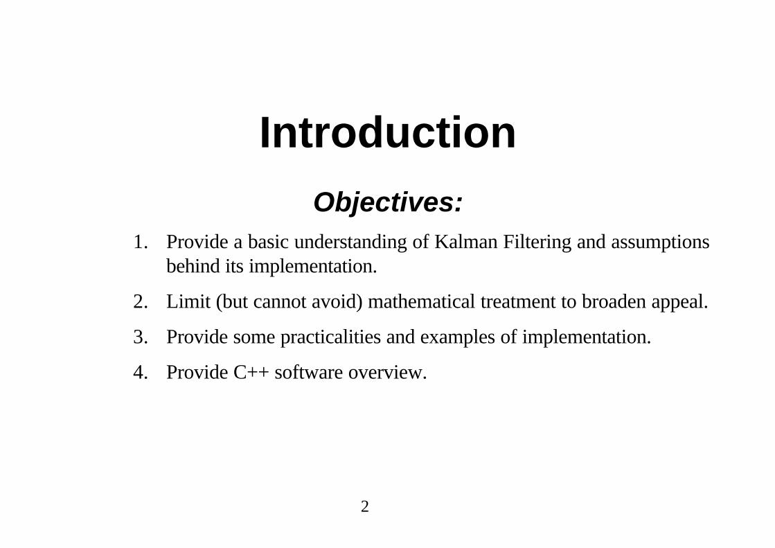
IntroductionObjectives:

1. Provide a basic understanding of Kalman Filtering and assumptionsbehind its implementation.

2. Limit (but cannot avoid) mathematical treatment to broaden appeal.

3. Provide some practicalities and examples of implementation.

4. Provide C++ software overview.

3

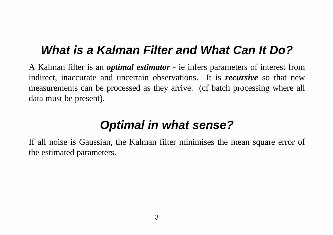
What is a Kalman Filter and What Can It Do?A Kalman filter is an optimal estimator - ie infers parameters of interest fromindirect, inaccurate and uncertain observations. It is recursive so that newmeasurements can be processed as they arrive. (cf batch processing where alldata must be present).

Optimal in what sense?If all noise is Gaussian, the Kalman filter minimises the mean square error ofthe estimated parameters.

4

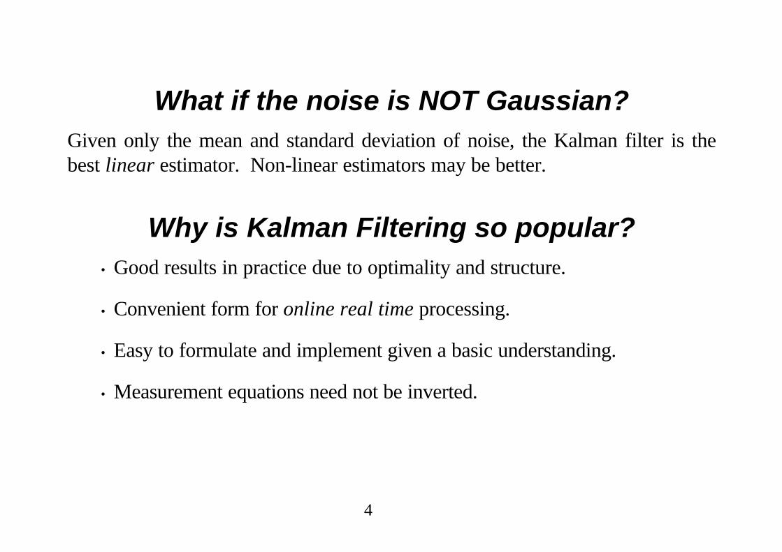
What if the noise is NOT Gaussian?Given only the mean and standard deviation of noise, the Kalman filter is thebest linear estimator. Non-linear estimators may be better.

Why is Kalman Filtering so popular?• Good results in practice due to optimality and structure.

• Convenient form for online real time processing.

• Easy to formulate and implement given a basic understanding.

• Measurement equations need not be inverted.

5

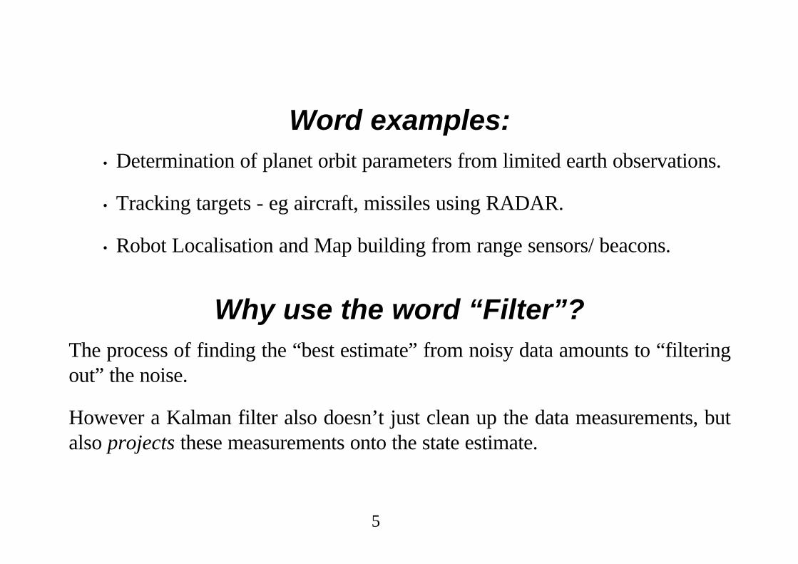
Word examples:• Determination of planet orbit parameters from limited earth observations.

• Tracking targets - eg aircraft, missiles using RADAR.

• Robot Localisation and Map building from range sensors/ beacons.

Why use the word “Filter”?The process of finding the “best estimate” from noisy data amounts to “filteringout” the noise.

However a Kalman filter also doesn’t just clean up the data measurements, butalso projects these measurements onto the state estimate.

6

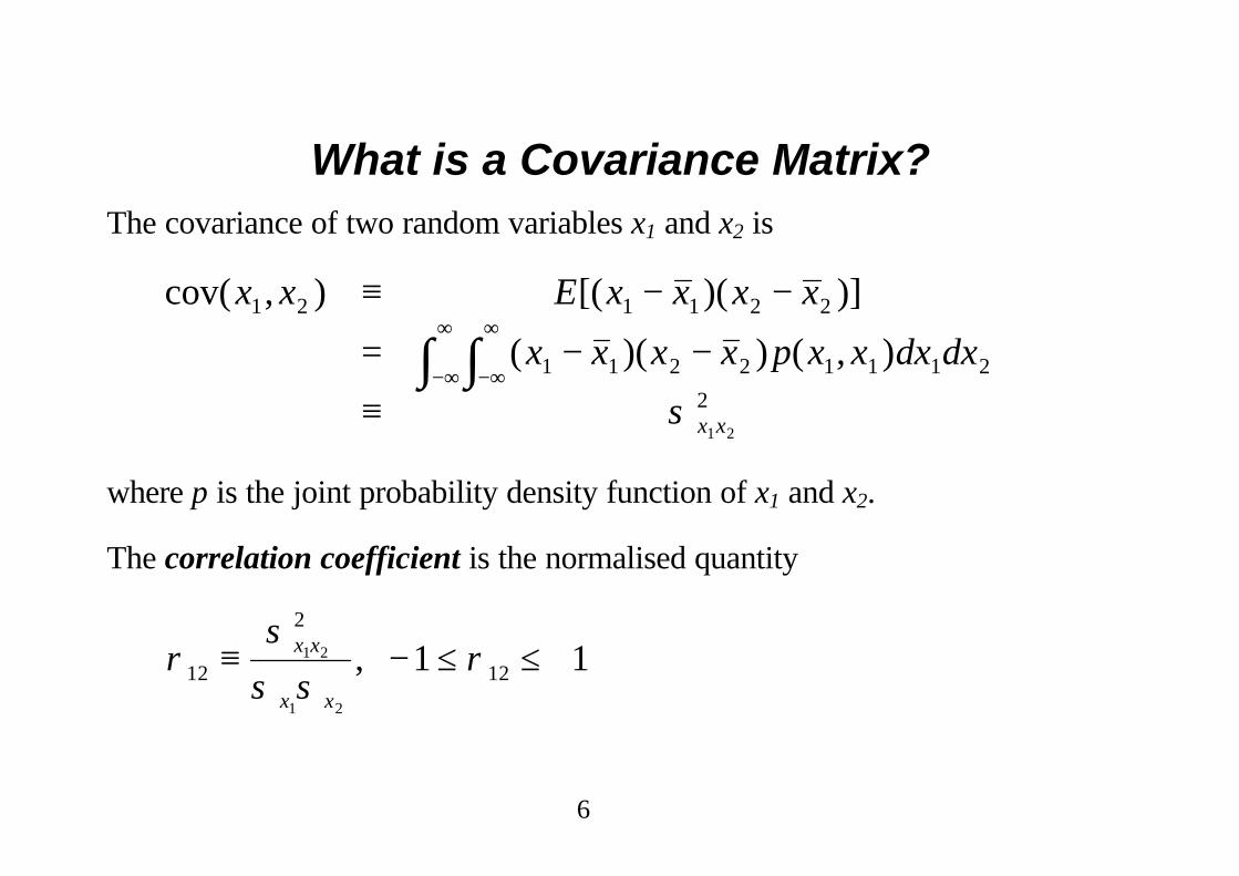
What is a Covariance Matrix?The covariance of two random variables x1 and x2 is

cov( , ) [( )( )]

( )( ) ( , )

x x E x x x x

x x x x p x x dx dx

x x

1 2 1 1 2 2

1 1 2 2 1 1 1 2

2

1 2

≡ − −

= − −

≡−∞

∞

−∞

∞

∫∫σ

where p is the joint probability density function of x1 and x2.

The correlation coefficient is the normalised quantity

ρσ

σ σρ12

2

121 2

1 2

1 1≡ − ≤ ≤ +x x

x x

,

7

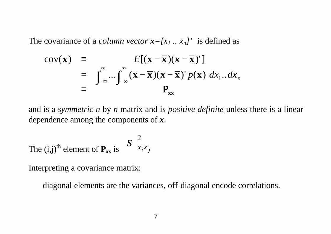
The covariance of a column vector x=[x1 .. xn]’ is defined as

cov( ) [( )( )' ]

... ( )( )' ( ) ..

x x x x x

x x x x x

Pxx

≡ − −

= − −≡

−∞

∞

−∞

∞

∫∫E

p dx dxn1

and is a symmetric n by n matrix and is positive definite unless there is a lineardependence among the components of x.

The (i,j)th element of Pxx is σ x xi j

2

Interpreting a covariance matrix:

diagonal elements are the variances, off-diagonal encode correlations.

8

Diagonalising a Covariance Matrixcov(x) is symmetric => can be diagonalised using an orthonormal basis.

By changing coordinates (pure rotation) to these unity orthogonal vectors weachieve decoupling of error contributions.

The basis vectors are the eigenvectors and form the axes of error ellipses.

The lengths of the axes are the square root of the eigenvalues and correspond tostandard deviations of the independent noise contribution in the direction of theeigenvector.

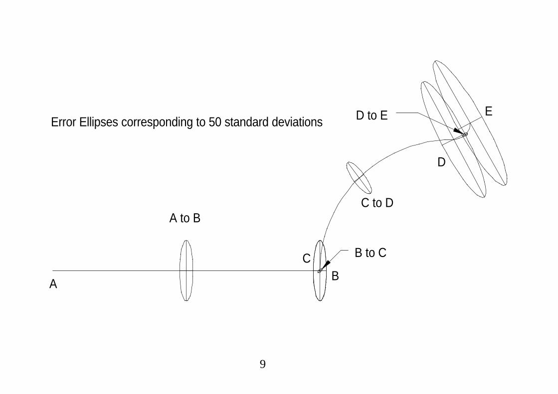
Example: Error ellipses for mobile robot odometry derived from covariancematrices:

9

A

Error Ellipses corresponding to 50 standard deviations

B

D

E

A to BC to D

B to C

D to E

C

10

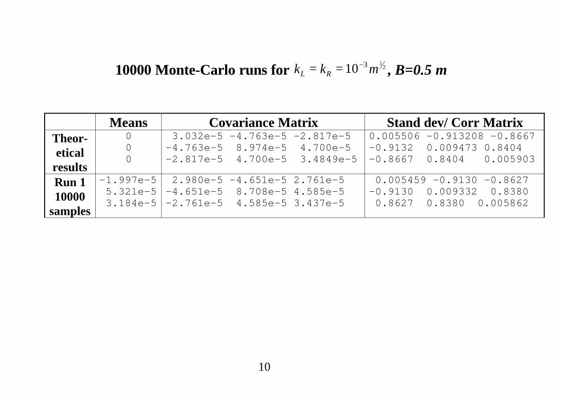
10000 Monte-Carlo runs for k k mL R= = −10 3 12 , B=0.5 m

Means Covariance Matrix Stand dev/ Corr MatrixTheor-etical

results

000

3.032e-5 -4.763e-5 -2.817e-5-4.763e-5 8.974e-5 4.700e-5-2.817e-5 4.700e-5 3.4849e-5

0.005506 -0.913208 -0.8667-0.9132 0.009473 0.8404-0.8667 0.8404 0.005903

Run 110000

samples

-1.997e-5 5.321e-5 3.184e-5

2.980e-5 -4.651e-5 2.761e-5-4.651e-5 8.708e-5 4.585e-5-2.761e-5 4.585e-5 3.437e-5

0.005459 -0.9130 -0.8627-0.9130 0.009332 0.8380 0.8627 0.8380 0.005862

11

Formulating a Kalman FilterProblem

We require discrete time linear dynamic system description by vectordifference equation with additive white noise that models unpredictabledisturbances.

STATE DEFINITION - the state of a deterministic dynamic system is thesmallest vector that summarises the past of the system in full.

Knowledge of the state allows theoretically prediction of the future (and prior)dynamics and outputs of the deterministic system in the absence of noise.

12

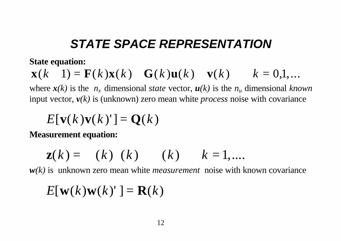
STATE SPACE REPRESENTATIONState equation:

x F x G u v( ) ( ) ( ) ( ) ( ) ( ) , , ...k k k k k k k+ = + + =1 0 1where x(k) is the nx dimensional state vector, u(k) is the nu dimensional knowninput vector, v(k) is (unknown) zero mean white process noise with covariance

E k k k[ ( ) ( )' ] ( )v v Q=Measurement equation:

z( ) ( ) ( ) ( ) ,....k k k k k= + = 1w(k) is unknown zero mean white measurement noise with known covariance

E k k k[ ( ) ( )' ] ( )w w R=

13

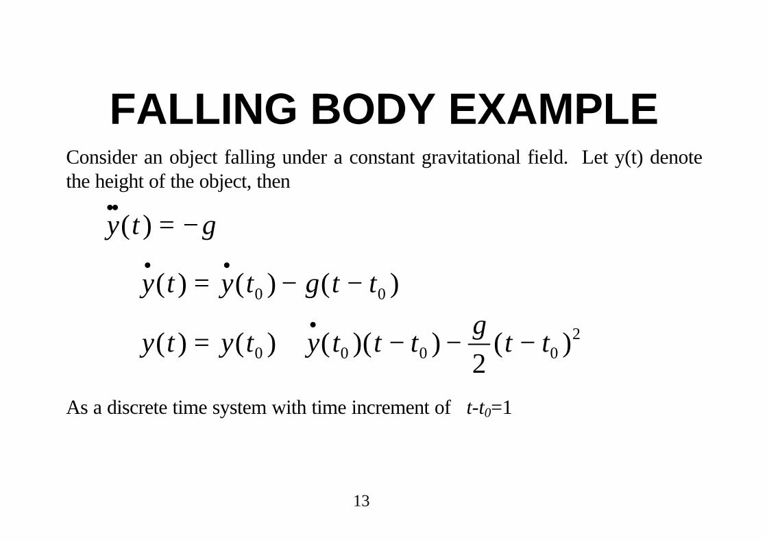
FALLING BODY EXAMPLEConsider an object falling under a constant gravitational field. Let y(t) denotethe height of the object, then

y t g

y t y t g t t

y t y t y t t tg

t t

... .

.

( )

( ) ( ) ( )

( ) ( ) ( )( ) ( )

= −

⇒ = − −

⇒ = + − − −

0 0

0 0 0 02

2

As a discrete time system with time increment of t-t0=1

14

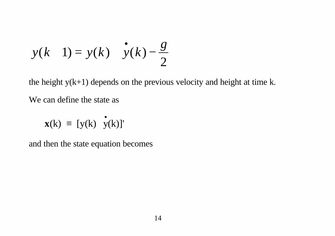
y k y k y kg

( ) ( ) ( ).

+ = + −12

the height y(k+1) depends on the previous velocity and height at time k.

We can define the state as

x(k) [y(k) y(k)]'.

≡

and then the state equation becomes

15

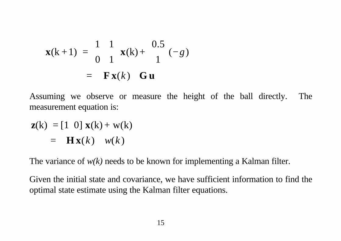
x x

F x G u

(k + 1) =1 1

0 1 (k) +

0.5

−

= +

1( )

( )

g

k

Assuming we observe or measure the height of the ball directly. Themeasurement equation is:

z x

H x

(k) = [1 0] (k) + w(k)

= +( ) ( )k w k

The variance of w(k) needs to be known for implementing a Kalman filter.

Given the initial state and covariance, we have sufficient information to find theoptimal state estimate using the Kalman filter equations.

16

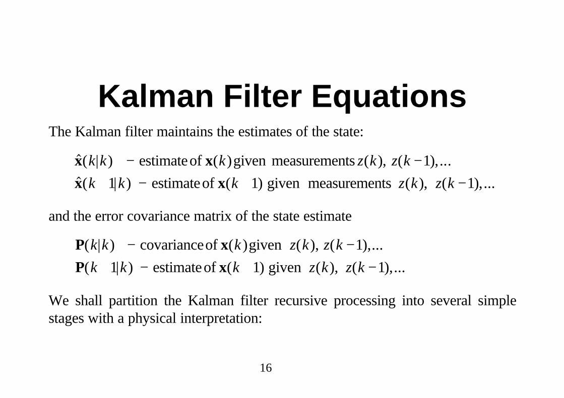
Kalman Filter EquationsThe Kalman filter maintains the estimates of the state:

$( | ) ( ) ( ), ( ),...

$( | ) ( ) ( ), ( ),...

x x

x x

k k k z k z k

k k k z k z k

− −+ − + −

estimateof given measurements

estimateof given measurements

1

1 1 1

and the error covariance matrix of the state estimate

P x

P x

( | ) ( ) ( ), ( ),...

( | ) ( ) ( ), ( ),...

k k k z k z k

k k k z k z k

− −+ − + −

covarianceof given

estimateof given

1

1 1 1

We shall partition the Kalman filter recursive processing into several simplestages with a physical interpretation:

17

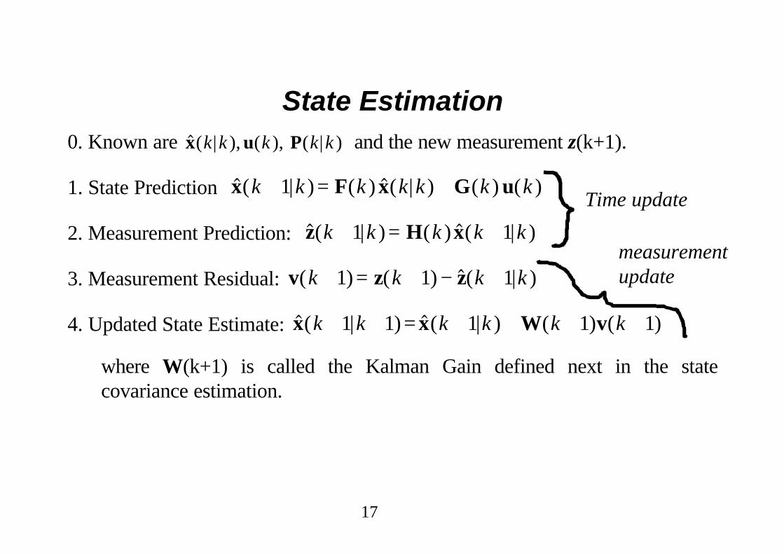
State Estimation0. Known are $ ( | ), ( ), ( | )x u Pk k k k k and the new measurement z(k+1).

1. State Prediction $( | ) ( ) $( | ) ( ) ( )x F x G uk k k k k k k+ = +1

2. Measurement Prediction: $( | ) ( ) $( | )z H xk k k k k+ = +1 1

3. Measurement Residual: v z z( ) ( ) $( | )k k k k+ = + − +1 1 1

4. Updated State Estimate: $( | ) $ ( | ) ( ) ( )x x W vk k k k k k+ + = + + + +1 1 1 1 1

where W(k+1) is called the Kalman Gain defined next in the statecovariance estimation.

Time update

measurementupdate

18

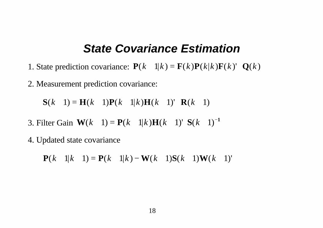
State Covariance Estimation1. State prediction covariance: P F P F Q( | ) ( ) ( | ) ( )' ( )k k k k k k k+ = +1

2. Measurement prediction covariance:

S H P H R( ) ( ) ( | ) ( )' ( )k k k k k k+ = + + + + +1 1 1 1 1

3. Filter Gain W P H S 1( ) ( | ) ( )' ( )k k k k k+ = + + + −1 1 1 1

4. Updated state covariance

P P W S W( | ) ( | ) ( ) ( ) ( )'k k k k k k k+ + = + − + + +1 1 1 1 1 1

19

Page 219 Bar-Shalom ANATOMY OF KALMAN FILTER

State at tk

x(k)

20

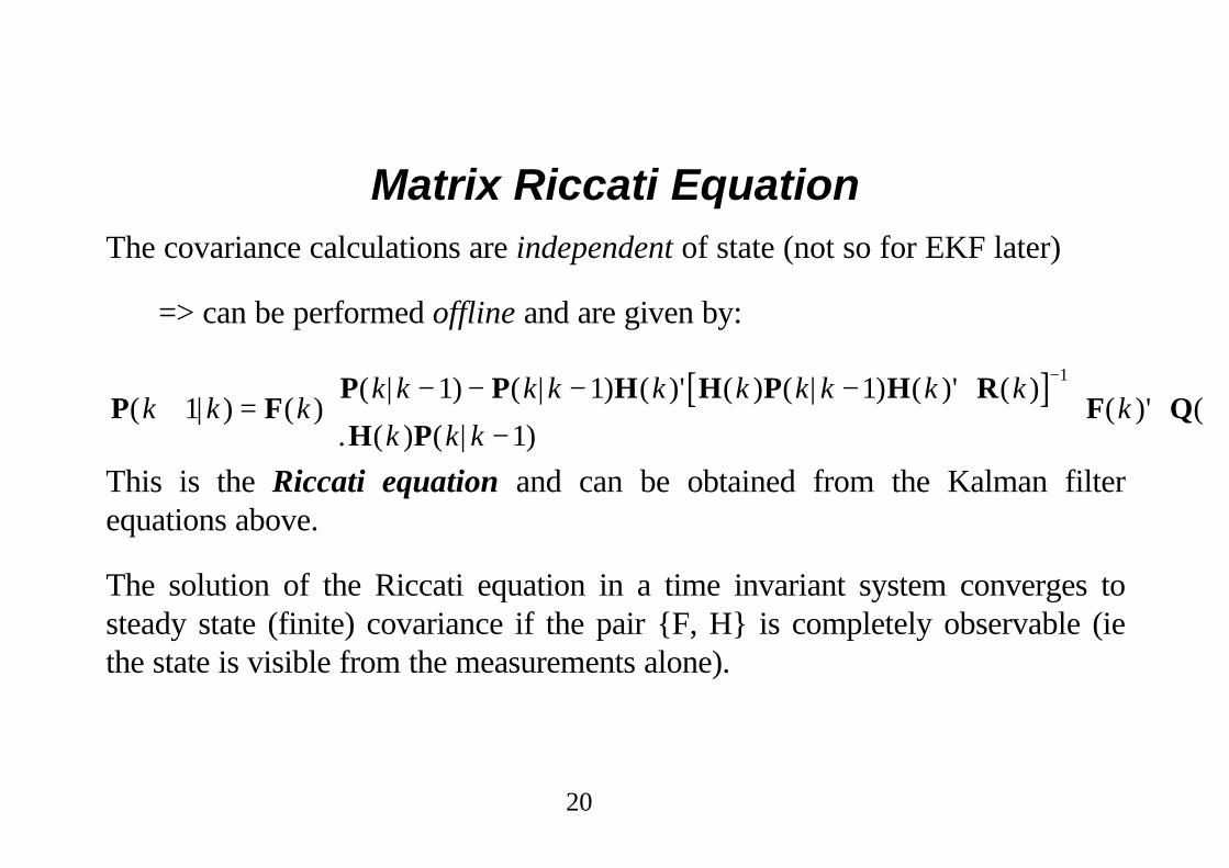
Matrix Riccati EquationThe covariance calculations are independent of state (not so for EKF later)

=> can be performed offline and are given by:

[ ]P FP P H H P H R

H PF Q( | ) ( )

( | ) ( | ) ( )' ( ) ( | ) ( )' ( )

. ( ) ( | )( )' (k k k

k k k k k k k k k k

k k kk+ =

− − − − +

−

+

−

11 1 1

1

1

This is the Riccati equation and can be obtained from the Kalman filterequations above.

The solution of the Riccati equation in a time invariant system converges tosteady state (finite) covariance if the pair {F, H} is completely observable (iethe state is visible from the measurements alone).

21

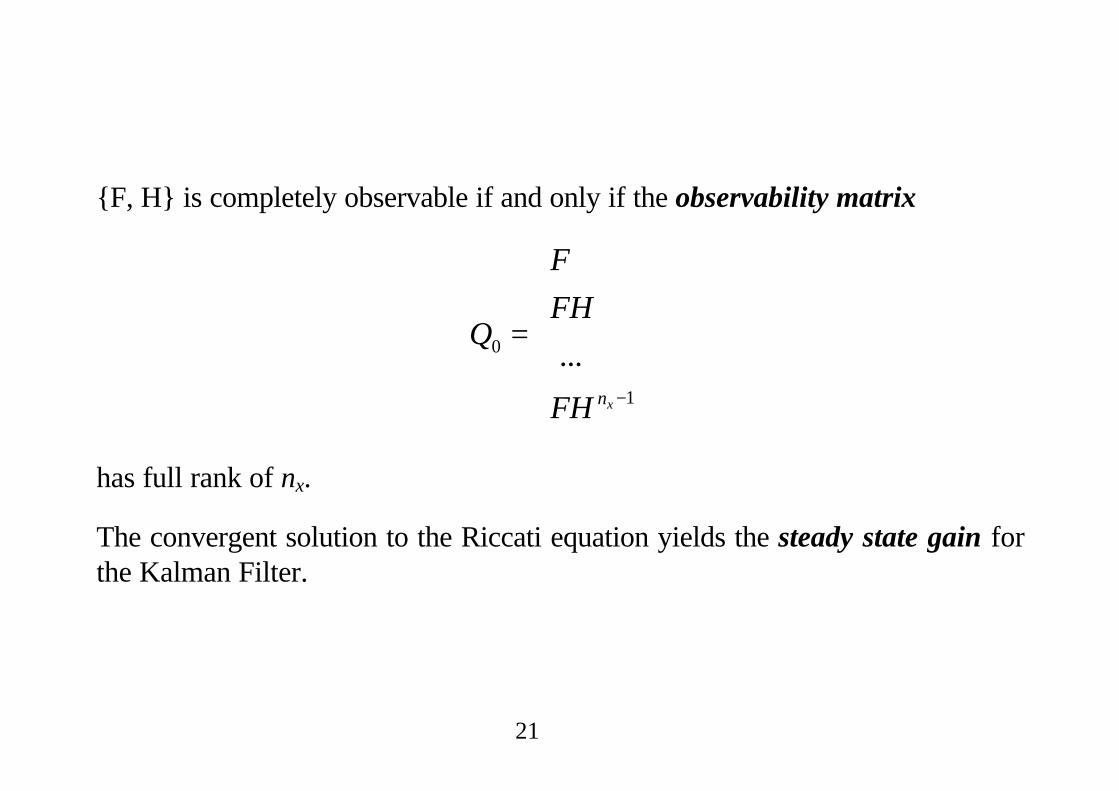
{F, H} is completely observable if and only if the observability matrix

Q

F

FH

FH nx

0

1

=

−

...

has full rank of nx.

The convergent solution to the Riccati equation yields the steady state gain forthe Kalman Filter.

22

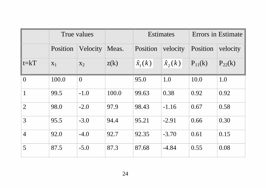
FALLING BODY KALMANFILTER (continued)

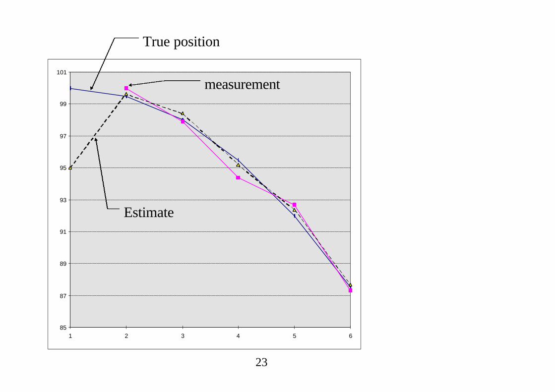
Assume an initial true state of position = 100 and velocity = 0, g=1.

We choose an initial estimate state estimate $( )x 0 and initial state covariance

P( )0 based on mainly intuition. The state noise covariance Q is all zeros.

The measurement noise covariance R is estimated from knowledge of predictedobservation errors, chosen as 1 here.

F, G, H are known the Kalman filter equations can be applied:

23

85

87

89

91

93

95

97

99

101

1 2 3 4 5 6

True position

Estimate

measurement

24

True values Estimates Errors in Estimate

Position Velocity Meas. Position velocity Position velocity

t=kT x1 x2 z(k) $ ( )x k1 $ ( )x k2 P11(k) P22(k)

0 100.0 0 95.0 1.0 10.0 1.0

1 99.5 -1.0 100.0 99.63 0.38 0.92 0.92

2 98.0 -2.0 97.9 98.43 -1.16 0.67 0.58

3 95.5 -3.0 94.4 95.21 -2.91 0.66 0.30

4 92.0 -4.0 92.7 92.35 -3.70 0.61 0.15

5 87.5 -5.0 87.3 87.68 -4.84 0.55 0.08

25

Kalman Filter Extensions• Validation gates - rejecting outlier measurements

• Serialisation of independent measurement processing

• Numerical rounding issues - avoiding asymmetric covariancematrices

• Non-linear Problems - linearising for the Kalman filter.

26

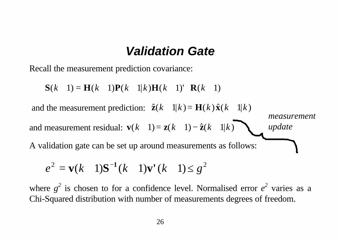
Validation GateRecall the measurement prediction covariance:

S H P H R( ) ( ) ( | ) ( )' ( )k k k k k k+ = + + + + +1 1 1 1 1

and the measurement prediction: $( | ) ( ) $( | )z H xk k k k k+ = +1 1

and measurement residual: v z z( ) ( ) $( | )k k k k+ = + − +1 1 1

A validation gate can be set up around measurements as follows:

e k k k g2 21 1 1= + + + ≤−v S v'1( ) ( ) ( )

where g2 is chosen to for a confidence level. Normalised error e2 varies as aChi-Squared distribution with number of measurements degrees of freedom.

measurementupdate

27

Sequential Measurement ProcessingIf the measurement noise vector components are uncorrelated then state updatecan be carried out one measurement at a time.

Thus matrix inversions are replaced by scalar inversions.

Procedure: state prediction as before

scalar measurements are processed sequentially (in any order)

using scalar measurement equations.

28

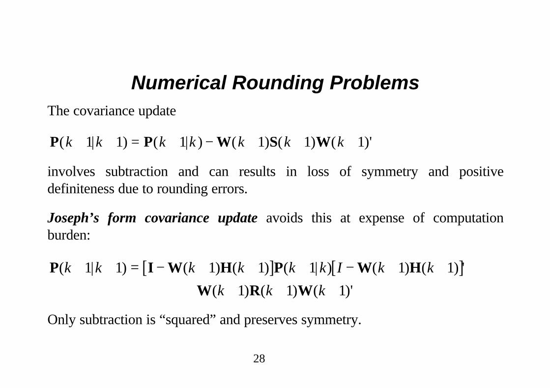
Numerical Rounding ProblemsThe covariance update

P P W S W( | ) ( | ) ( ) ( ) ( )'k k k k k k k+ + = + − + + +1 1 1 1 1 1

involves subtraction and can results in loss of symmetry and positivedefiniteness due to rounding errors.

Joseph’s form covariance update avoids this at expense of computationburden:

[ ] [ ]P I W H P W H

W R W

( | ) ( ) ( ) ( | ) ( ) ( ) '

( ) ( ) ( )'

k k k k k k I k k

k k k

+ + = − + + + − + ++ + + +

1 1 1 1 1 1 1

1 1 1

Only subtraction is “squared” and preserves symmetry.

29

Extended Kalman Filter (EKF)Many practical systems have non-linear state update or measurement equations.The Kalman filter can be applied to a linearised version of these equations withloss of optimality:

30

EKF - p 387 Bar-Shalom

31

Iterated Extended Kalman Filter (IEKF)The EKF linearised the state and measurement equations about the predictedstate as an operating point. This prediction is often inaccurate in practice.

The estimate can be refined by re-evaluating the filter around the new estimatedstate operating point. This refinement procedure can be iterated until littleextra improvement is obtained - called the IEKF.

32

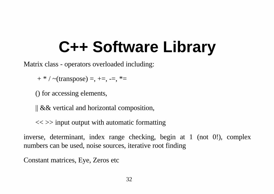
C++ Software LibraryMatrix class - operators overloaded including:

+ * / ~(transpose) =, +=, -=, *=

() for accessing elements,

|| && vertical and horizontal composition,

<< >> input output with automatic formatting

inverse, determinant, index range checking, begin at 1 (not 0!), complexnumbers can be used, noise sources, iterative root finding

Constant matrices, Eye, Zeros etc

33

Kalman filtering classes, for defining and implementing KF, EKF and IEKF

-allows numerical checking of Jacobian functions

Software source is available to collaborators for non-commercial use providedappropriately acknowledged in any publication. Standard disclaimers apply!

contact Lindsay.Kleeman@monash.edu.au

34

Further ReadingBar-Shalom and Xiao-Rong Li, Estimation and Tracking: Principles,Techniques and Software, Artech House Boston, 1993.

Jazwinski, A. H. . Stochastic Processes and Filtering Theory. New York,Academic Press, 1970.

Bozic, S M, Digital and Kalman Filtering, Edward Arnold, London 1979.

Maybeck, P. S. “The Kalman filter: An introduction to concepts.” AutonomousRobot Vehicles. I. J. Cox and G. T. Wilfong. New York, Springer-Verlag: 194-204, 1990.

35

Odometry Error Covariance Estimation for TwoWheel Robot Vehicles (Technical Report MECSE-95-1, 1995)

A closed form error covariance matrix is developed for(i) straight lines and(ii) constant curvature arcs(iii) turning about the centre of axle of the robot.

Other paths can be composed of short segments of constant curvature arcs.

Assumes wheel distance measurement errors are zero mean white noise.

Previous work incrementally updates covariance matrix in small times steps.

36

Our approach integrates noise over the entire path for a closed form errorcovariance - more efficient and accurate

37

Scanned Monocular Sonar SensingSmall ARC project 1995 - aims:

• To investigate a scanned monocular ultrasonic sensor capable of high speedmultiple object range and bearing estimation.

• Deploy the sensor in these robotic applications:• obstacle avoidance,• doorway traversal and docking operations,• localisation and mapping.