Embed Size (px)
Citation preview

Digital Object Identifier 10.1109/MCS.2009.935569
66 IEEE CONTROL SYSTEMS MAGAZINE » APRIL 2010 1066-033X/10/$26.00©2010IEEE
Kalman Filtering in Wireless Sensor Networks
ALEJANDRO RIBEIRO, IOANNIS D. SCHIZAS, STERGIOS I. ROUMELIOTIS, and GEORGIOS B. GIANNAKIS
wireless sensor network (WSN) is a collection
of physically distributed sensing devices that
can communicate through a shared wireless
channel. Sensors can be deployed, for example,
to detect the presence of a contaminant in a
water reservoir, to estimate the temperature in an orange
grove, or to track the position of a moving target.
The promise of WSNs stems from the benefits of distrib-
uted sensing and control. For example, in the target-tracking
setup depicted in Figure 1, where sensors measure their
distance to a target whose trajectory is to be estimated, the
benefit of distributed sensing is the availability of observa-
tions with high signal-to-noise ratio (SNR). Whether col-
lected by a passive radar, which estimates distances by the
strength of an electromagnetic signature emitted by the
target, or by an active radar, which gauges the reflection of
a probing signal, measured signal strength decreases with
increasing distance. Observation noise, however, remains
unchanged because it is determined by circuit design and
the operational environment. Consequently, in passive and
active radar, the SNR of distance observations is inversely
related to the distance being measured. In a conventional
radar system a few expensive stations are deployed to cover
a substantial area. Most of the time, the distance between
the target and the sensors is large, and the observation SNR
is low. Since the WSN comprises a large number of sensors,
at each point in time a few sensors are close to the target,
and thus measured distances are smaller. Although the cir-
cuitry of the sensors in the WSN is of lower quality than
that of stations in a conventional radar system of compara-
ble cost, the decrease in SNR due to the larger circuit noise
power is more than offset by the smaller distances mea-
sured. Therefore, a WSN offers the potential to reduce
localization error.
WSNs offer several advantages beyond those inherent to
their distributed nature. Because sensors are independent
hardware units, the likelihood of a large number of them
REDUCING COMMUNICATION COST IN STATE-ESTIMATION PROBLEMS
AFABIO BUCCIARELLI
Authorized licensed use limited to: University of Minnesota. Downloaded on April 10,2010 at 21:25:18 UTC from IEEE Xplore. Restrictions apply.
APRIL 2010 « IEEE CONTROL SYSTEMS MAGAZINE 67
failing simultaneously is small. Thus, WSNs have built-in
redundancy, which can improve robustness relative to cen-
tralized processing. Redundancy also simplifies network
deployment because optimizing sensor placements is not
critical. Considering also the fact that it is not necessary to
wire the sensors together, network deployment can be as
simple as scattering the sensors over the area of interest.
See [2]–[4] for discussions of additional advantages, issues,
and applications of WSNs.
Although WSNs present attractive features, challenges
associated with the scarcity of bandwidth and power in
wireless communications have to be addressed. For the
state-estimation problems discussed here, observations
about a common state are collected by physically distrib-
uted terminals. To perform state estimation, sensors may
share these observations with each other or communicate
them to a fusion center for centralized processing. In either
scenario, the communication cost in terms of bandwidth
and power required to convey observations is large enough
to merit attention. To explore this point, consider a vector
state x (n) [ Rp at time n and let the kth sensor collect
observations yk(n) [ Rq. The linear state and observation
models are
x (n) 5 A (n)x (n 2 1) 1 u (n) , (1)
yk(n) 5 Hk(n)x (n) 1 vk(n) , (2)
where the driving noise vector u (n) is normal and uncor-
related across time with covariance matrix Cu (n) , while
the normal observation noise vk(n) has covariance matrix
Cv (n) and is uncorrelated across time and sensors.
With K vector observations 5yk(n)6k51K available, the
optimal mean squared error (MSE) estimation of the state
x (n) for the linear model (1), (2) is accomplished by a
Kalman filter. Brute force collection of these observations,
however, incurs a communication cost commensurate with
the product of the number K of sensors in the network, the
number of scalar observations in the yk(n) vectors, and the
number of bits used to quantize each component of yk(n) .
The communication cost incurred by brute force collec-
tion of observations is not only large but unnecessary. It is
possible to reduce the impact of the three factors mentioned
above by exploiting information redundancy across obser-
vations yk1(n) and yk2
(n) collected by different sensors,
between different scalar observations composing the vector
yk(n) at a given sensor, and within each individual scalar
observation. Indeed, because all sensors are observing the
same state x (n) , the measurements yk1(n) and yk2
(n) are
correlated. As a consequence of this correlation, it is possi-
ble for sensor k1 to estimate the observation of sensor k2
and use this estimate to reduce the cost of communicating
its own observation to k2. The correlation between individ-
ual components of the vector observation yk(n) can be
exploited to group scalar observations in a vector of reduced
dimensionality. Finally, it is not necessary to finely quan-
tize components of yk(n) but only to the extent that further
precision in the quantization of yk(n) contributes to reduc-
ing the error in the estimation of the state x (n) .
To reduce the cost of communicating the components of
yk(n) , we discuss filters that estimate the state x (n) based
on quantized representations of the original observations
yk(n) using a small number of bits, typically between one
and three. Finely quantized versions of yk(n) can be used
in lieu of the nonquantized observations yk in standard
Kalman filters. This substitution is not possible with
coarsely quantized versions, motivating the design of state
estimators that incorporate the nonlinear quantization
operation into the observation model. The challenge in this
estimation problem is that the quantization operator is dis-
continuous. In principle, it is therefore necessary to resort
to nonlinear state-estimation tools, such as the unscented
Kalman filter [5] or the particle filter [6], resulting in pro-
hibitive computational cost for WSN deployment. However,
it turns out that despite the discontinuous observation
model it is possible to build state-estimation algorithms
whose structure and computational cost is similar to a
standard Kalman filter. These algorithms are presented in
the section “Quantized Kalman Filters.”
We begin by considering quantization to a single bit by
resorting to the transmission of the sign of the innovations
sequence. Quantization to multiple bits is addressed
through an iterative quantizer. Whereas coarse quantiza-
tion to a few bits per observation increases the MSE of esti-
mates relative to a Kalman filter using finely quantized
observations, performance analysis of quantized Kalman
filters shows that the increase in MSE is small. As we detail
in the section “Quantized Kalman Filters,” quantization to
a single bit per observation increases the MSE by a factor of
p/2 < 1.57 with respect to a standard Kalman filter, while
quantization to 2 bits and 3 bits results in relative penalties
of 1.15 and 1.05; see also [7] and [8]. Applications of quan-
tized Kalman filters using 1 bit and 3 bits per observation are
presented for a simulated target-tracking problem and an
experimental multiple robot localization problem.
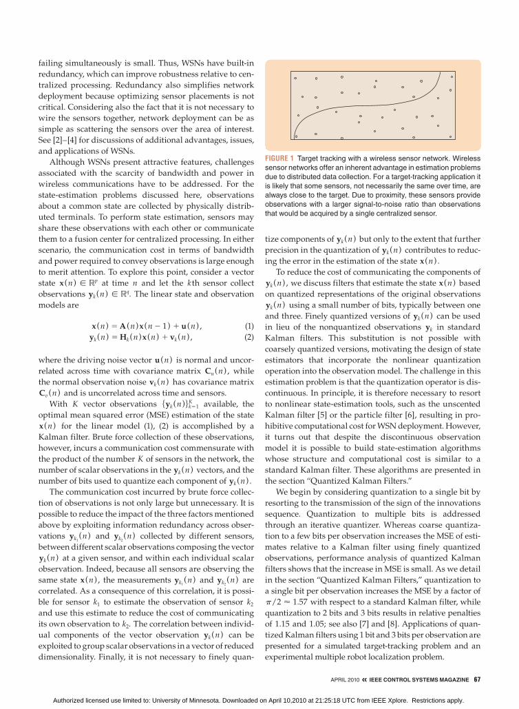
FIGURE 1 Target tracking with a wireless sensor network. Wireless
sensor networks offer an inherent advantage in estimation problems
due to distributed data collection. For a target-tracking application it
is likely that some sensors, not necessarily the same over time, are
always close to the target. Due to proximity, these sensors provide
observations with a larger signal-to-noise ratio than observations
that would be acquired by a single centralized sensor.
Authorized licensed use limited to: University of Minnesota. Downloaded on April 10,2010 at 21:25:18 UTC from IEEE Xplore. Restrictions apply.
68 IEEE CONTROL SYSTEMS MAGAZINE » APRIL 2010
To exploit the correlation between observation data
acquired at different sensors, recursive data-aggregation
protocols are discussed. Brute force collection of yk(n)
observations incurs a large communication cost because,
in addition to transmitting their own observations, sen-
sors transmit observations received from other sensors in
previous communications. Instead of forwarding separate
observations, sensors forward linear combinations of
their local information with messages received from
neighboring sensors, which are also linear combinations
formed at earlier times. State estimation in this context
calls for the design of MSE optimal estimators for x (n)
based on recursive linear combinations of data. To this
end, the section “Consensus-Based Distributed Kalman
Filtering and Smoothing” describes how to design the
messages exchanged among sensors and the information-
combining rules.
Finally, the correlation between components of yk(n)
allows sensors to reduce the dimensionality of their obser-
vation data yk(n) . The compression procedure is designed
to trade off transmission cost as dictated by the reduced
dimension and estimation accuracy as quantified by the
MSE. Given a limited power budget available at each sensor
and the fact that communication takes place over nonideal
channel links, the goal is to design linear dimensionality-
reducing operators that minimize the state-estimate MSE
when operating over noisy channels. Two scenarios are con-
sidered, differentiated by whether state estimation takes
place at a fusion center or at predetermined sensors in an ad
hoc topology.
The reader interested on technical details can find a
brief literature guide in “Further Reading.”
QUANTIZED KALMAN FILTERSTo study quantized Kalman filters we initially focus on
scalar observations 5yk(n)6k51K , resulting in an observation
model of the form yk(n) 5 hkT (n)x (n) 1 vk(n) with noise
variance sv (n) . We also assume that a scheduling algo-
rithm is in place to decide which sensor is to transmit at
time n. Therefore, with k (n) denoting the scheduled sensor
at time n, an efficient means of quantizing and transmit-
ting y (n) J yk(n) (n) is sought. In more precise terms we
study state-estimation problems when nonquantized
amplitude observations y (n) are mapped to messages
m (n) containing a small number of bits.
Quantization results in a subtle change in the state-es-
timation problem. Instead of seeking the minimum mean
squared error (MMSE) estimator x (n|y0:n ) based on past
observations y0:n J 3y (0) , c, y (n)4T, the problem trans-
mutes into that of finding the MMSE estimator x (n|m0:n )
based on past messages m0:n J 3m (0) ,c, m (n)4T. Al-
though both estimators are given by the respective condi-
tional means, the use of past observations yields a
canonical linear-state estimation, whereas the use of past
messages is a challenging nonlinear estimation. Since the
computational cost of most nonlinear state-estimation
review of research challenges associated with WSNs can be
found in [3]. Comprehensive references dealing with various
applications and research problems are included in [2] and [S1].
The sign of innovations Kalman fi lter is presented in [7]. From
a more general point of view, the intermingling of quantization
and estimation has a long history; early references include [S2]
and [S3]. In the context of wireless sensor networks, the prob-
lem is revisited in [S4]–[S6]. An introduction to this topic can be
found in [S7]. The iterative sign of innovations Kalman fi lter is
developed in [S8]. More general quantization rules for Kalman
fi ltering problems can be found in [8]. The distributed Kalman
smoother state estimators can be found in [24], whereas alter-
native distributed implementations are available in [15]–[17] and
[19]. Detailed treatment of distributed computation and estima-
tion are given in [22], [24], and [29], and the references therein.
The intertwining of dimensionality reduction with estimation and
tracking is further developed in [12], [31], [S7], and [S8].
REFERENCES[S1] S. Kumar, F. Zao, and D. Shepherd, Eds., IEEE Signal Processing Mag. (Special Issue on Collaborative Information Processing), vol. 19,
no. 2, Mar. 2002.
[S2] R. Curry, W. Vandervelde, and J. Potter, “Nonlinear estimation with
quantized measurements—PCM, predictive quantization, and data
compression,” IEEE Trans. Inform. Theory, vol. 16, no. 2, pp. 152–161,
Mar. 1970.
[S3] D. Williamson, “Finite wordlength design of digital Kalman fi lters
for state estimation,” IEEE Trans. Automat. Contr., vol. 30, no. 10, pp.
930–939, Oct. 1985.
[S4] H. Papadopoulos, G. Wornell, and A. Oppenheim, “Sequential sig-
nal encoding from noisy measurements using quantizers with dynamic
bias control,” IEEE Trans. Inform. Theory, vol. 47, no. 3, pp. 978–1002,
Mar. 2001.
[S5] A. Ribeiro and G. B. Giannakis, “Bandwidth-constrained distrib-
uted estimation for wireless sensor networks, Part I: Gaussian case,”
IEEE Trans. Signal Processing, vol. 54, no. 3, pp. 1131–1143, Mar.
2006.
[S6] A. Ribeiro and G. B. Giannakis, “Bandwidth-constrained distrib-
uted estimation for wireless sensor networks, Part II: Unknown pdf,”
IEEE Trans. Signal Processing, vol. 54, no. 7, pp. 2784–2796, July
2006.
[S7] J.-J. Xiao, A. Ribeiro, Z.-Q. Luo, and G. B. Giannakis, “Distributed com-
pression-estimation using wireless sensor networks,” IEEE Signal Process-ing Mag., vol. 23, no. 4, pp. 27–41, July 2006.
[S8] I. D. Schizas, G. B. Giannakis, and Z. Q. Luo, “Distributed
estimation using reduced-dimensionality sensor observations,”
IEEE Trans. Signal Processing, vol. 55, no. 8, pp. 4284–4299, Aug.
2007.
Further Reading
A
Authorized licensed use limited to: University of Minnesota. Downloaded on April 10,2010 at 21:25:18 UTC from IEEE Xplore. Restrictions apply.
APRIL 2010 « IEEE CONTROL SYSTEMS MAGAZINE 69
algorithms is excessive for WSN deployments, the goal is
to find filters that can deal with quantization discontinui-
ties while retaining the small computational requirements
and memory footprints of conventional Kalman filters.
These properties are present in the sign of innovations
Kalman filter (SOI-KF) and its variants discussed in this
section; see also [7].
Sign of Innovations Kalman FilterIn state-estimation problems, the innovations sequence is
defined as the difference between the current observation
and its prediction based on past observations. The intuition
supporting this definition is that this difference contains
the information that the current observation y (n) has
about the state x (n) that is not conveyed by previous
observations y0:n21. It is thus natural to define the predicted
estimates as y (n|m0:n21 ) J E 3y (n)|m0:n21 4, the corre-
sponding innovations sequence as y| (n|m0:n21 ) J y (n) 2
y (n|m0:n21 ) , and the message m (n) as a quantized version
of y| (n|m0:n21 ) . As a first approach, consider quantization
to a single bit per observation and let messages exchanged
consist of the sign of the innovations sequence, that is,
m(n) J sign 3y| (n|m0:n21) 45 sign 3y (n) 2 y (n|m0:n21 ) 4. The
sequence m (n) indicates whether the observation y (n) is
larger or smaller than the prediction y (n|m0:n21 ) based on
past messages m0:n21.
The estimation task at hand is then to find the MMSE
estimate x (n|m0:n ) of the state x (n) given the current and
past messages m0:n. The MMSE estimate is given by the
conditional expectation E 3x (n)|m0:n 4, which in principle
can be determined by computing the corresponding multi-
dimensional integral of the state x (n) weighted by the
conditional distribution p 3x (n)|m0:n 4 of the state, given
messages m0:n. Evaluating this integral, in turn, requires
knowing the probability density function (pdf) p 3x (n)|m0:n 4, which can be found using the prediction-correction algo-
rithm described below.
The prediction step involves obtaining the predic tion
pdf p 3x (n)|m0:n21 4 from the correction pdf p 3x (n 2 1) 0 m0:n21 4. The state x (n) at time n is the sum of A (n)x (n 2 1)
and the independent input noise u (n) . Therefore, to
obtain the prediction pdf p 3x (n)|m0:n21 4, it suffices to
propagate the correction pdf p 3x (n 2 1)|m0:n21 4 through
the linear transformation A (n) and then convolve the
result with the normal pdf N 3u (n) ; 0, Cu (n)4 of the driv-
ing noise.
The correction step starts from the prediction pdf and
com putes the correction pdf p 3x (n)|m0:n 4. This computation
can be done by applying Bayes’s rule to the random vari-
ables x (n) and m (n) to obtain
p 3x (n)|m0:n 45 p 3x (n)|m0:n21 4Pr5m (n)|x (n), m0:n216Pr5m (n)|m0:n216 .
(3)
In spirit, these prediction-correction steps are not
different from the corresponding ones in the Kalman
filter. With linear state propagation, linear observations,
normal driving inputs, and normal observation noise,
the prediction pdfs p 3x (n)|y0:n21 4 and the correction
pdfs p 3x (n)|y0:n21 4 are normal. As such, prediction and
correction pdfs are completely characterized by their
means and covariances, which are the quantities that
the Kalman filter tracks. Thus, the prediction step in the
Kalman filter can be interpreted as propagating the cor-
rection pdf p 3x (n 2 1)|y0:n21 4 of the previous step to the
prediction pdf p 3x (n)|y0:n21 4 through convolution. Like-
wise, the correction step uses Bayes’s rule to obtain the
correction pdf p 3x (n)|y0:n 4 from the prediction pdf
p 3x (n)|y0:n21 4. Because quantization is a nonlinear operation, the
probability distributions p 3x (n)|m0:n21 4 and p 3x (n)|m0:n 4 necessary to find x (n|m0:n ) are not normal. Conse-
quently, it is not sufficient to track their first two moments,
and the prediction-correction becomes computationally
costly. An alternative approximation in nonlinear filter-
ing (see [9]) is to model the prediction pdf p 3x (n)|m0:n21 4 as normal so that, at least for the prediction step, only the
mean and covariance must be propagated as performed
by (see also Figure 2 )
x (n|m0:n21) 5 A (n) x (n 2 1|m0:n21 ) , (4)
M(n|m0:n21) 5 A (n)M (n21|m0:n21 )AT (n) 1Cu (n) . (5)
Even with this simplifying approximation, p 3x (n)|m0:n 4 is
not normal. Indeed, the probability Pr5m (n)|x (n) , m0:n216 of observing m (n) given the state x (n) and past obser-
vations m0:n21 can be rewritten as Pr5m (n)|x (n) 6 because conditioning on past messages given the present
state is redundant. Furthermore, m (n) 5 1 is equivalent to
y (n) 2 y (n|m0:n21 ) $ 0, which, using the observation
model in (2), yields hT (n)x (n) 2 y (n|m0:n21 ) $ v (n) . Sim-
ilarly, m (n) 5 21 is equivalent to y (n) 2 y (n|m0:n21 ) , 0
and, from the observation model, to hT (n)x (n) 2
y (n|m0:n21 ) , v (n) . Given that the observation noise
v (n) is normal, the probability of v (n) being larger or
smaller than hT (n)x (n) 2 y (n|m0:n21 ) can be expressed
in terms of the normal cumulative distribution function.
Comparing these comments with Bayes’s rule (3), we
deduce that p 3x (n)|m0:n21 4 is the product of the normal
pdf p 3x (n)|m0:n21 4 and the normal cumulative distri-
bution Pr5m (n)|x (n) , m0:n216. The remaining term
Pr5m (n) 0 m0:n216 is a normalizing constant.
While the correction pdf in (3) is not normal, the
MMSE estimate is nonetheless obtained as the solution
of the expected value integral, which could be evaluated
numerically. It is noteworthy, however, that a closed-
form expression for this integral exists and leads to the
correction step [7]
Authorized licensed use limited to: University of Minnesota. Downloaded on April 10,2010 at 21:25:18 UTC from IEEE Xplore. Restrictions apply.
70 IEEE CONTROL SYSTEMS MAGAZINE » APRIL 2010
x (n|m0:n ) 5 x (n|m0:n21 )
1("2/p )M (n|m0:n21 )h (n)
"hT (n)M (n|m0:n21 )h (n) 1 sv2 (n)
m (n) ,
(6)
M (n|m0:n ) 5 M (n|m0:n21 )
2(2/p )M (n|m0:n21)h (n)hT (n)M (n|m0:n21)
hT (n)M (n|m0:n21)h (n) 1sv2 (n)
.
(7)
The SOI-KF, which amounts to a recursive application of
(4), (5) and (6), (7), is similar to the Kalman filter in that it
requires only a few algebraic operations per iteration.
Moreover, comparison of the SOI-KF covariance correction
equation with the corresponding covariance correction for
the standard Kalman filter based on the innovations reveals
that they are identical except for the factor 2/p.
The similarity between the covariance updates of the
Kalman filter and the SOI-KF allows for a simple perfor-
mance comparison. The variance of the state estimates
increases with each prediction step and decreases with
each correction step. Starting with the same covariance
matrix M (n 2 1|m0:n21 ) 5 M (n 2 1|y0:n21 ) at time n 2 1,
a Kalman filter and an SOI-KF have identical predicted
covariance matrices, that is, M (n|m0:n21 ) 5 M (n|y0:n21 ) ,
at time n. To compare the corrected variances of the
Kalman filter and the SOI-KF, it is informative to examine
the per-step covariance reductions. For the Kalman filter,
the per-step covariance reduction is defined as DMKF(n) JM (n 2 1 0 y0:n21 ) 2 M (n|y0:n ) , while, for the SOI-KF, it is
defined as DM (n) J M (n 2 1|m0:n21 ) 2 M (n|m0:n ) . It is
not difficult to recognize that these reductions are related
by the factor 2/p, that is, DM (n) 5 (2/p )DMKF(n) .
Using the sign of innovations m (n) thus entails a penalty
of 1 2 2/p 5 36% relative to the variance reduction
afforded by the actual innovations y (n) . This penalty is
−4 −2 0 2 4 60
0.05
0.1
0.15
0.2
0.25
0.3
0.35
x (n) x (n)
x (n) x (n)
(a) (b)
(c) (d)
Pre
dic
ted p
df
Prediction pdfNormal Approx.
0 1 2 3 4 5 60
0.1
0.2
0.3
0.4
0.5
Corr
ecte
d p
df
−6 −4 −2 0 2 40
0.05
0.1
0.15
0.2
0.25
0.3
Pre
dic
ted p
df
−6 −4 −2 0 20
0.1
0.2
0.3
0.4
Corr
ecte
d p
df
Correction pdfNormal Approx.
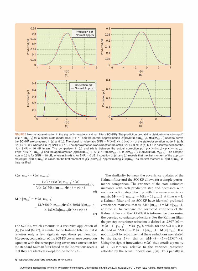
FIGURE 2 Normal approximation in the sign of innovations Kalman filter (SOI-KF). The prediction probability distribution function (pdf)
p 3x (n ) |m0: n21 4 for a scalar state model x (n ) 5 x (n ) and the normal approximation N 3x (n ) ; x (n |m0:n21), M(n|m0:n21)4 used to derive
the SOI-KF are compared in (a) and (b). The signal to noise ratio SNR J h2(n )E 3x2(n ) 4/sv2(n ) of the state-observation model in (a) is
SNR 5 10 dB, whereas in (b) SNR 5 0 dB. The approximation works best for the small SNR 5 0 dB in (b) but it is accurate even for the
high SNR 5 10 dB in (a). The comparison in (c) and (d) is between the actual correction pdf p 3x (n ) |m0:n 4 ~ p 3x (n ) |m0:n21 4 Pr5m(n ) |x (n ) , m0:n216 and the approximation p| 3x (n ) |m0:n 4 ~ N 3x (n ) ; x (n|m0:n21) , M(n|m0:n21)4Pr 5m(n ) |x (n ) , m0:n216. The compar-
ison in (c) is for SNR 5 10 dB, whereas in (d) is for SNR 5 0 dB. Inspection of (c) and (d) reveals that the first moment of the approxi-
mated pdf p| 3x (n ) |m0:n 4 is similar to the first moment of p 3x (n ) |m0:n 4. Approximating x (n|m0:n) as the first moment of p| 3x (n ) |m0:n 4 is
thus justified.
Authorized licensed use limited to: University of Minnesota. Downloaded on April 10,2010 at 21:25:18 UTC from IEEE Xplore. Restrictions apply.
APRIL 2010 « IEEE CONTROL SYSTEMS MAGAZINE 71
modest for the use of a coarse quantization rule of one bit
per scalar observation.
On the other hand, while 2/p relates the per-step covari-
ance reductions, these reductions accumulate over time and
eventually could cause considerable loss in SOI-KF perfor-
mance relative to the Kalman filter. Therefore, while the rela-
tive penalty of using the sign of the innovations in lieu of the
actual innovation is small, the absolute penalty could be con-
siderable. These limitations motivate consideration of finer
multibit quantization rules, which are discussed below.
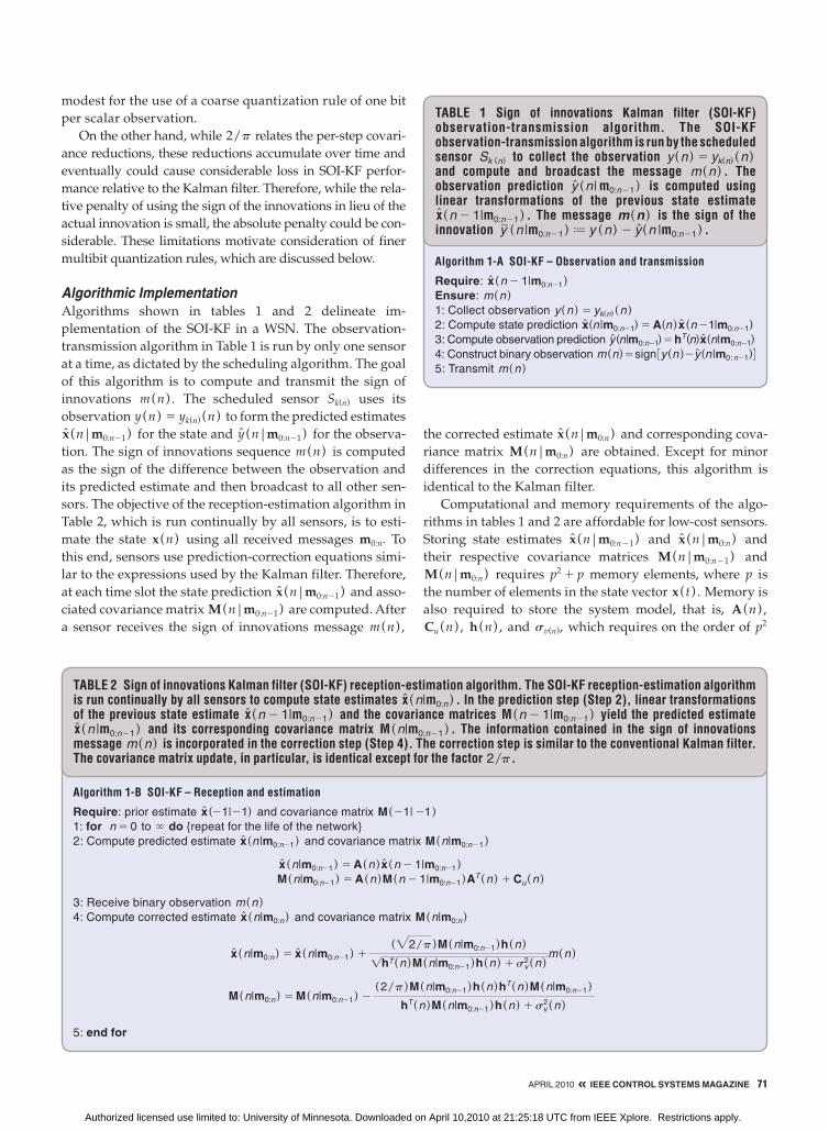
Algorithmic ImplementationAlgorithms shown in tables 1 and 2 delineate im -
plementation of the SOI-KF in a WSN. The observation-
transmission algorithm in Table 1 is run by only one sensor
at a time, as dictated by the scheduling algorithm. The goal
of this algorithm is to compute and transmit the sign of
innovations m (n) . The scheduled sensor Sk(n) uses its
observation y (n) 5 yk(n) (n) to form the predicted estimates
x (n|m0:n21 ) for the state and y (n|m0:n21 ) for the observa-
tion. The sign of innovations sequence m (n) is computed
as the sign of the difference between the observation and
its predicted estimate and then broadcast to all other sen-
sors. The objective of the reception-estimation algorithm in
Table 2, which is run continually by all sensors, is to esti-
mate the state x (n) using all received messages m0:n. To
this end, sensors use prediction-correction equations simi-
lar to the expressions used by the Kalman filter. Therefore,
at each time slot the state prediction x (n|m0:n21 ) and asso-
ciated covariance matrix M (n|m0:n21 ) are computed. After
a sensor receives the sign of innovations message m (n) ,
the corrected estimate x (n|m0:n ) and corresponding cova-
riance matrix M (n|m0:n ) are obtained. Except for minor
differences in the correction equations, this algorithm is
identical to the Kalman filter.
Computational and memory requirements of the algo-
rithms in tables 1 and 2 are affordable for low-cost sensors.
Storing state estimates x (n|m0:n21 ) and x (n|m0:n ) and
their respective covariance matrices M (n|m0:n21 ) and
M (n|m0:n ) requires p2 1 p memory elements, where p is
the number of elements in the state vector x ( t ) . Memory is
also required to store the system model, that is, A (n) ,
Cu (n) , h (n) , and sv(n), which requires on the order of p2
Algorithm 1-A SOI-KF – Observation and transmission
Require: x (n 2 1|m0:n21)
Ensure: m(n )
1: Collect observation y (n ) 5 yk(n) (n )
2: Compute state prediction x(n|m0:n21) 5 A(n ) x (n 21|m0:n21)
3: Compute observation prediction y (n|m0:n21)5 hT(n)x(n|m0:n21)
4: Construct binary observation m(n)5sign 3y (n )2y (n|m0:n21)4 5: Transmit m(n )
TABLE 1 Sign of innovations Kalman filter (SOI-KF) observation-transmission algorithm. The SOI-KF observation-transmission algorithm is run by the scheduled sensor Sk (n) to collect the observation y (n) 5 yk(n) (n) and compute and broadcast the message m(n) . The observation prediction y (n| m0:n21 ) is computed using linear transformations of the previous state estimate x (n 2 1|m0:n21 ) . The message m(n ) is the sign of the innovation y| (n |m0:n21 ) J y (n) 2 y (n |m0:n21 ) .
Algorithm 1-B SOI-KF – Reception and estimation
Require: prior estimate x (21|21) and covariance matrix M(21| 21 )
1: for n 5 0 to ` do {repeat for the life of the network}
2: Compute predicted estimate x (n|m0:n21) and covariance matrix M(n|m0:n21)
x (n|m0:n21) 5 A(n ) x (n 2 1|m0:n21)
M(n|m0:n21) 5 A(n )M(n 2 1|m0:n21)AT(n ) 1 Cu(n )
3: Receive binary observation m(n )
4: Compute corrected estimate x (n|m0:n) and covariance matrix M(n|m0:n)
x (n|m0:n) 5 x (n|m0:n21) 1("2/p )M(n|m0:n21)h(n )
!hT(n )M(n|m0:n21)h(n ) 1 sv2(n )
m(n )
M(n|m0:n) 5 M(n|m0:n21) 2(2/p )M(n|m0:n21)h(n )hT(n )M(n|m0:n21)
hT(n )M(n|m0:n21)h(n ) 1 sv2(n )
5: end for
TABLE 2 Sign of innovations Kalman filter (SOI-KF) reception-estimation algorithm. The SOI-KF reception-estimation algorithm is run continually by all sensors to compute state estimates x (n|m0:n ) . In the prediction step (Step 2), linear transformations of the previous state estimate x (n 2 1|m0:n21 ) and the covariance matrices M (n 2 1|m0:n21 ) yield the predicted estimate x (n |m0:n21 ) and its corresponding covariance matrix M (n|m0:n21 ) . The information contained in the sign of innovations message m(n) is incorporated in the correction step (Step 4). The correction step is similar to the conventional Kalman filter. The covariance matrix update, in particular, is identical except for the factor 2/p.
Authorized licensed use limited to: University of Minnesota. Downloaded on April 10,2010 at 21:25:18 UTC from IEEE Xplore. Restrictions apply.
72 IEEE CONTROL SYSTEMS MAGAZINE » APRIL 2010
memory elements. Prediction equations (4) and (5) require
p2 and p3 flops, respectively. Correction equations (6) and
(7) necessitate on the order of p2 flops and, in the case of (6),
the computation of a scalar square root. The latter opera-
tion is the only one that is not shared with a Kalman filter
based on the actual innovations y| (n|m0:n21 ) .
Because the scheduled sensor Sk(n) also runs the recep-
tion-estimation algorithm in Table 2, it does not take full
advantage of the information that yk(n) (n) contains about
the state x (n) . In principle, sensors not scheduled at time n
could improve performance of their estimates by combin-
ing their own observations yk(n) . Local information is
left out from the algorithms in tables 1 and 2 because the
goal of the SOI-KF is to obtain a synchronized estimate
x (n|m0:n ) across all sensors.
Filter ImplementationWhile the MSE updates of the Kalman filter and its
quantized version in (7) are similar, the update of the state
estimates has a different form. As it turns out, it is possible
to express the state update in (6) in a form that exemplifies
its link with the Kalman filter update. By replacing the
innovation y| (n|m0:n21 ) with its sign m (n) , the units of
the observations are lost. To recover these units, let
s,y (n|m0:n21 ) J !E 3y|2 (n|m0:n21 )4 denote the standard
deviation of the innovations sequence and define the
SOI-KF innovation as m| (n|m0:n21 ) J sy| (n|m0:n21 )m (n) .
The innovation sequence has zero-mean and its variance is
given by the denominator of the MSE update in (7).
According to this definition, the units of the SOI-KF
innovation m| (n|m0:n21 ) are those of y| (n|m0:n21 ) , and their
average energies are the same, that is, E 3m|2 (n|m0:n21 )45
E 3y|2 (n|m0:n21 )4. Recalling the definition of the Kalman gain and replac-
ing m (n) with m| (n|m0:n21 ) in (6), the SOI-KF takes a form
more reminiscent of the Kalman filter
k (n) JM (n|m0:n21 )h (n)
hT (n)M (n|m0:n21 )h (n) 1 sv2 (n)
, (8)
x (n|m0:n ) 5 x (n|m0:n21 ) 1 ("2/p )k (n)m| (n|m0:n21 ) ,
(9)
M (n|m0:n ) 5 3I 2 (2/p )k (n)hT (n)4 M (n|m0:n21 ) . (10)
The gain k (n) in (8) has the same functional expression as
the gain used in the Kalman filter, while the MSE updates
are identical except for the factor 2/p. The state updates
differ only in the factor !2/p and in the replacement of
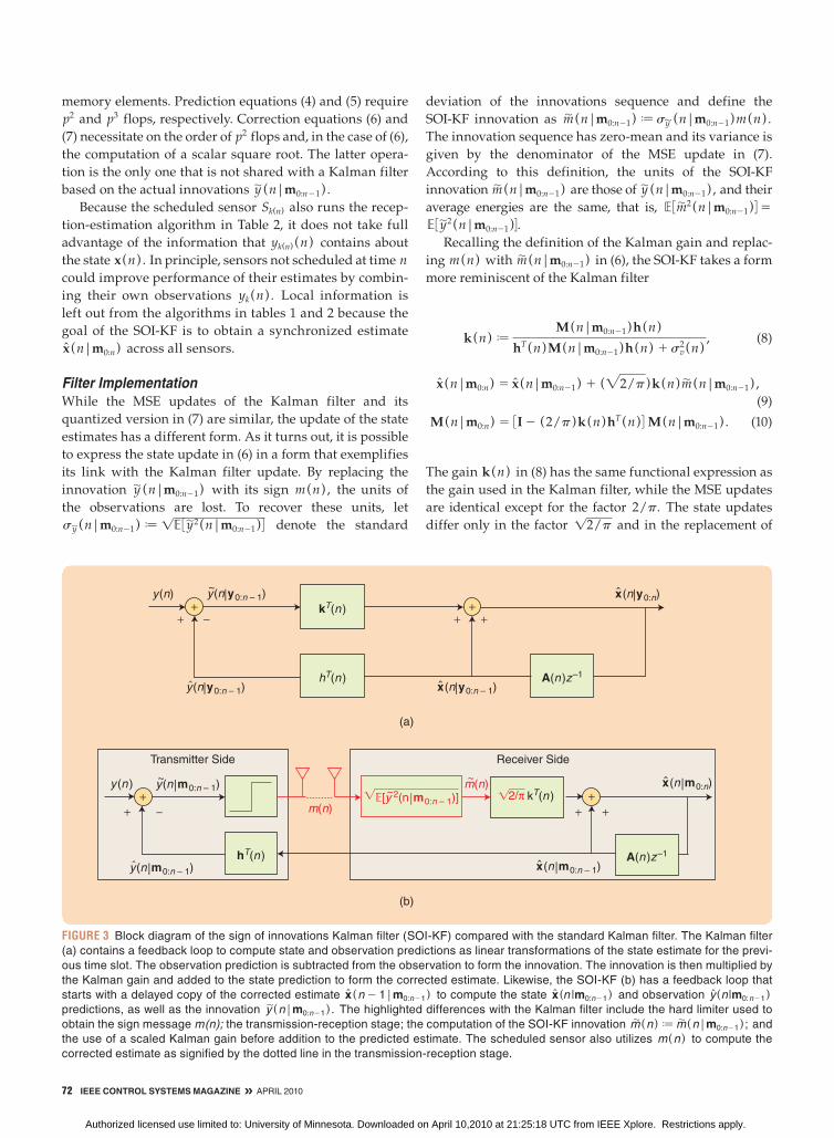
FIGURE 3 Block diagram of the sign of innovations Kalman filter (SOI-KF) compared with the standard Kalman filter. The Kalman filter
(a) contains a feedback loop to compute state and observation predictions as linear transformations of the state estimate for the previ-
ous time slot. The observation prediction is subtracted from the observation to form the innovation. The innovation is then multiplied by
the Kalman gain and added to the state prediction to form the corrected estimate. Likewise, the SOI-KF (b) has a feedback loop that
starts with a delayed copy of the corrected estimate x (n 2 1|m0:n21) to compute the state x (n |m0:n21) and observation y (n|m0:n21)
predictions, as well as the innovation y|(n|m0:n21) . The highlighted differences with the Kalman filter include the hard limiter used to
obtain the sign message m(n); the transmission-reception stage; the computation of the SOI-KF innovation m|(n ) J m| (n|m0:n21) ; and
the use of a scaled Kalman gain before addition to the predicted estimate. The scheduled sensor also utilizes m(n ) to compute the
corrected estimate as signified by the dotted line in the transmission-reception stage.
y(n) y(n|y0:n – 1)~
x(n|y0:n – 1)^y(n|y0:n – 1)^
x(n|y0:n)^
kT(n )
hT(n ) A(n )z–1
+ ++ ++ −
(a)
(b)
y(n |m0:n – 1)~
y(n |m0:n – 1) x(n |m0:n – 1)^^
x(n |m0:n)^
hT(n )
y (n )
A(n )z–1
+ +++ − +
Transmitter Side Receiver Side
m(n)
m(n)~
E[y 2(n |m0:n – 1)]! kT(n )2/π!
~
Authorized licensed use limited to: University of Minnesota. Downloaded on April 10,2010 at 21:25:18 UTC from IEEE Xplore. Restrictions apply.
APRIL 2010 « IEEE CONTROL SYSTEMS MAGAZINE 73
the innovation y| (n|m0:n21 ) by the SOI-KF innovation
m| (n|m0:n21 ) . As the first- and second-order moments of
y| (n|m0:n21 ) and m| (n|m0:n21 ) are identical, the factor
!2/p appearing in the state update explains the factor
2/p in the MSE update. The difference between the SOI-KF
correction and the Kalman filter correction is that in the
SOI-KF the magnitude of the correction at each step is
determined by the magnitude of s,y (n|m0:n21 ) , which is
the same regardless of how large or small the actual inno-
vation y| (n|m0:n21 ) is.
Expressing the correction step as in (8), (10) simplifies
the comparison between the block diagrams of the Kalman
filter and the SOI-KF. The block diagram for the Kalman
filter in Figure 3 includes the feedback loop on the right
that starts with a delayed copy of the corrected estimate
x (n 2 1|y0:n21 ) and computes the predicted estimate
x (n|y0:n21 ) along with the observation prediction
y (n|y0:n21 ) . The observation prediction is then subtracted
from the observation y (n) to compute the innovation
y| (n|y0:n21 ) . The innovation is then multiplied by the
Kalman gain k (n) and added to the predicted estimate to
yield the corrected estimate x (n|y0:n ) . The block diagram
for the SOI-KF in Figure 3 contains the same feedback loop
that starts with a delayed copy of the corrected estimate
x (n 2 1|m0:n21 ) to compute state x (n|m0:n21 ) and obser-
vation y (n|m0:n21 ) predictions as well as the innovation
y| (n|m0:n21 ) . The SOI-KF passes the innovation through a
hard limiter to obtain the sign message m (n) , which is then
broadcast to other sensors. Upon reception, the message
m (n) is multiplied by the innovation’s variance to yield the
SOI-KF innovation m| (n|m0:n21 ) . The innovation is then
multiplied by a scaled Kalman gain and added to the pre-
dicted estimate to yield the corrected estimate x (n|m0:n ) .
The scheduled sensor also utilizes m (n) to compute the
corrected estimate as signified by the dotted line in the
transmission-reception stage.
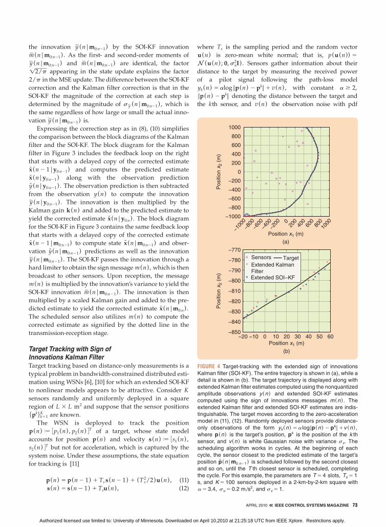
Target Tracking with Sign of Innovations Kalman FilterTarget tracking based on distance-only measurements is a
typical problem in bandwidth-constrained distributed esti-
mation using WSNs [6], [10] for which an extended SOI-KF
to nonlinear models appears to be attractive. Consider K
sensors randomly and uniformly deployed in a square
region of L 3 L m2 and suppose that the sensor positions
5pk6k51K are known.
The WSN is deployed to track the position
p (n) J 3p1 (n) , p2 (n) 4T of a target, whose state model
accounts for position p (n) and velocity s (n) J 3s1 (n) ,
s2 (n) 4T but not for acceleration, which is captured by the
system noise. Under these assumptions, the state equation
for tracking is [11]
p (n) 5 p (n 2 1) 1 Ts s (n 2 1) 1 (Ts2/2)u (n) , (11)
s (n) 5 s (n 2 1) 1 Tsu (n) , (12)
where Ts is the sampling period and the random vector
u (n) is zero-mean white normal; that is, p (u (n)) 5
N(u (n) ; 0, su2I ) . Sensors gather information about their
distance to the target by measuring the received power
of a pilot signal following the path-loss model
yk(n) 5 alog 7p (n) 2 pk 7 1 v (n) , with constant a $ 2,
7p (n) 2 pk 7 denoting the distance between the target and
the kth sensor, and v (n) the observation noise with pdf
−100
0
−800
−600
−400
−200 0
200
400
600
80010
00−1000
−800
−600
−400
−200
0
200
400
600
800
1000
Positio
n x
2 (
m)
Position x1 (m)
Position x1 (m)
(a)
(b)
Positio
n x
2 (
m)
−20 −10 0 10 20 30 40 50 60−850
−840
−830
−820
−810
−800
−790
−780
−770
Sensors Target
Extended Kalman
FilterExtended SOI−KF
FIGURE 4 Target-tracking with the extended sign of innovations
Kalman filter (SOI-KF). The entire trajectory is shown in (a), while a
detail is shown in (b). The target trajectory is displayed along with
extended Kalman filter estimates computed using the nonquantized
amplitude observations y (n ) and extended SOI-KF estimates
computed using the sign of innovations messages m(n ) . The
extended Kalman filter and extended SOI-KF estimates are indis-
tinguishable. The target moves according to the zero-acceleration
model in (11), (12). Randomly deployed sensors provide distance-
only observations of the form yk (n ) 5 a log 7p(n ) 2 pk 7 1v (n ) ,
where p(n ) is the target’s position, pk is the position of the k th
sensor, and v (n ) is white Gaussian noise with variance sv. The
scheduling algorithm works in cycles. At the beginning of each
cycle, the sensor closest to the predicted estimate of the target’s
position p(n|m0:n21) is scheduled followed by the second closest
and so on, until the T th closest sensor is scheduled, completing
the cycle. For this example, the parameters are T 5 4 slots, Ts 5 1
s, and K 5 100 sensors deployed in a 2-km-by-2-km square with
a 5 3.4, su 5 0.2 m/s2, and sv 5 1.
Authorized licensed use limited to: University of Minnesota. Downloaded on April 10,2010 at 21:25:18 UTC from IEEE Xplore. Restrictions apply.
74 IEEE CONTROL SYSTEMS MAGAZINE » APRIL 2010
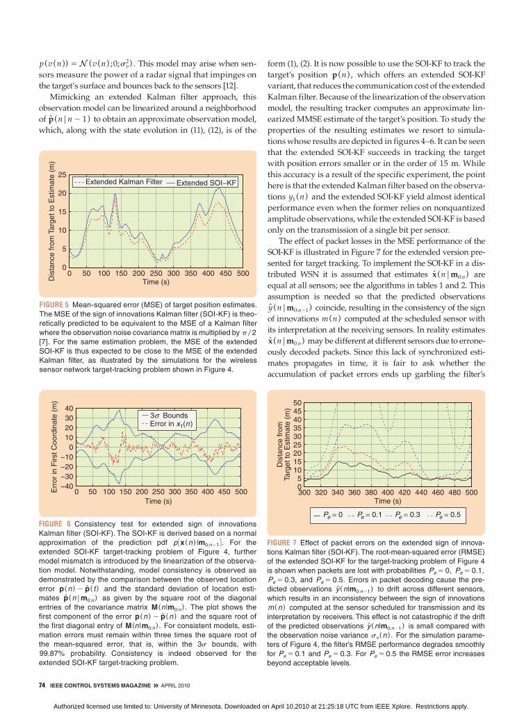
p (v (n)) 5N(v (n) ;0;sv2 ) . This model may arise when sen-
sors measure the power of a radar signal that impinges on
the target’s surface and bounces back to the sensors [12].
Mimicking an extended Kalman filter approach, this
observation model can be linearized around a neighborhood
of p (n|n 2 1) to obtain an approximate observation model,
which, along with the state evolution in (11), (12), is of the
form (1), (2). It is now possible to use the SOI-KF to track the
target’s position p (n) , which offers an extended SOI-KF
variant, that reduces the communication cost of the extended
Kalman filter. Because of the linearization of the observation
model, the resulting tracker computes an approximate lin-
earized MMSE estimate of the target’s position. To study the
properties of the resulting estimates we resort to simula-
tions whose results are depicted in figures 4–6. It can be seen
that the extended SOI-KF succeeds in tracking the target
with position errors smaller or in the order of 15 m. While
this accuracy is a result of the specific experiment, the point
here is that the extended Kalman filter based on the observa-
tions yk(n) and the extended SOI-KF yield almost identical
performance even when the former relies on nonquantized
amplitude observations, while the extended SOI-KF is based
only on the transmission of a single bit per sensor.
The effect of packet losses in the MSE performance of the
SOI-KF is illustrated in Figure 7 for the extended version pre-
sented for target tracking. To implement the SOI-KF in a dis-
tributed WSN it is assumed that estimates x (n|m0:n ) are
equal at all sensors; see the algorithms in tables 1 and 2. This
assumption is needed so that the predicted observations
y (n|m0:n21 ) coincide, resulting in the consistency of the sign
of innovations m (n) computed at the scheduled sensor with
its interpretation at the receiving sensors. In reality estimates
x (n|m0:n ) may be different at different sensors due to errone-
ously decoded packets. Since this lack of synchronized esti-
mates propagates in time, it is fair to ask whether the
accumulation of packet errors ends up garbling the filter’s
0 50 100 150 200 250 300 350 400 450 5000
5
10
15
20
25
Time (s)Dis
tance fro
m T
arg
et to
Estim
ate
(m
)
Extended Kalman Filter Extended SOI−KF
FIGURE 5 Mean-squared error (MSE) of target position estimates.
The MSE of the sign of innovations Kalman filter (SOI-KF) is theo-
retically predicted to be equivalent to the MSE of a Kalman filter
where the observation noise covariance matrix is multiplied by p/2
[7]. For the same estimation problem, the MSE of the extended
SOI-KF is thus expected to be close to the MSE of the extended
Kalman filter, as illustrated by the simulations for the wireless
sensor network target-tracking problem shown in Figure 4.
0 50 100 150 200 250 300 350 400 450 500−40
−30
−20
−10
0
10
20
30
40
Time (s)
Err
or
in F
irst C
oord
inate
(m
)
3σ BoundsError in x1(n )
FIGURE 6 Consistency test for extended sign of innovations
Kalman filter (SOI-KF). The SOI-KF is derived based on a normal
approximation of the prediction pdf p 3x (n ) |m0:n21 4. For the
extended SOI-KF target-tracking problem of Figure 4, further
model mismatch is introduced by the linearization of the observa-
tion model. Notwithstanding, model consistency is observed as
demonstrated by the comparison between the observed location
error p(n ) 2 p( t ) and the standard deviation of location esti-
mates p(n|m0:n) as given by the square root of the diagonal
entries of the covariance matrix M(n|m0:n) . The plot shows the
first component of the error p(n ) 2 p(n ) and the square root of
the first diagonal entry of M(n|m0:n) . For consistent models, esti-
mation errors must remain within three times the square root of
the mean-squared error, that is, within the 3s bounds, with
99.87% probability. Consistency is indeed observed for the
extended SOI-KF target-tracking problem.
300 320 340 360 380 400 420 440 460 480 50005
101520253035404550
Time (s)
Dis
tance fro
mTarg
et to
Estim
ate
(m
)
Pe = 0 Pe = 0.1 Pe = 0.3 Pe = 0.5
FIGURE 7 Effect of packet errors on the extended sign of innova-
tions Kalman filter (SOI-KF). The root-mean-squared error (RMSE)
of the extended SOI-KF for the target-tracking problem of Figure 4
is shown when packets are lost with probabilities Pe 5 0, Pe 5 0.1,
Pe 5 0.3, and Pe 5 0.5. Errors in packet decoding cause the pre-
dicted observations y (n|m0:n21) to drift across different sensors,
which results in an inconsistency between the sign of innovations
m(n ) computed at the sensor scheduled for transmission and its
interpretation by receivers. This effect is not catastrophic if the drift
of the predicted observations y (n|m0:n21) is small compared with
the observation noise variance sv (n ) . For the simulation parame-
ters of Figure 4, the filter’s RMSE performance degrades smoothly
for Pe 5 0.1 and Pe 5 0.3. For Pe 5 0.5 the RMSE error increases
beyond acceptable levels.
Authorized licensed use limited to: University of Minnesota. Downloaded on April 10,2010 at 21:25:18 UTC from IEEE Xplore. Restrictions apply.
APRIL 2010 « IEEE CONTROL SYSTEMS MAGAZINE 75
output. Figure 7 shows that lost packets have a mild effect on
the filter’s performance by showing the MSE for the extended
SOI-KF when packet error probabilities Pe vary between 0
and 0.3. Small and moderate error probabilities Pe 5 0.1 and
Pe 5 0.3 have a noticeable but not catastrophic effect on the
MSE of the filter. When the packet error probability is Pe 5 0.5,
the MSE error increases beyond acceptable levels. The resil-
iency of the filter is maintained as long as the drift of predicted
observations y (n|m0:n21 ) is small compared with the obser-
vation noise variance sv (n) .
Iterative Sign of Innovations Kalman FilterConsider now a general quantization scenario, where the
scheduled sensor at time n broadcasts an L-bit message
m(n) with entry m(l) (n) denoting the lth bit. As with the
SOI-KF, it is natural to consider quantization of the innova-
tions sequence y| (n|m0:n21 ) , where having l bits broadens
the set of possible quantizers. A simple idea is to transmit
the L most significant bits of the innovation, but this
approach is suboptimal since it amounts to uniform quanti-
zation of y| (n|m0:n21 ) , whose distribution is close to normal.
An optimal quantizer for y| (n|m0:n21 ) is not difficult to
design using Lloyd’s algorithm, an idea developed to con-
struct quantized Kalman filters in [8].
Alternatively, we can build on the simplicity of the
SOI-KF recursions by designing an iterative means for select-
ing the individual bits as signs of an extended innovation
sequence [8]. More precisely, let m(l) (n) J 3m(1) (n) , c,
m(l) (n)4T denote the first l bits of the message m(n) and
define y(l) (n|m0:n21 ) J E 3y (n)|m(l) (n) , m0:n21 4, which is
the observation estimate given past messages and the
first l bits of the current message. By convention,
y(0) (n|m0:n21 ) J E 3y (n)|m0:n21 4 is the observation esti-
mate given past messages only. An extended innovations
sequence can then be defined, where each observation
y (n) generates L terms. When the observation y (n)
becomes available, the innovation y|(1) (n|m0:n21 ) J y (n) 2
y(0) (n|m0:n21 ) is first defined followed by y|(2) (n|m0:n21 ) J
y (n) 2 y(1) (n|m0:n21 ) . This process is repeated L times,
and at the lth step the innovation y|(l) (n|m0:n21 ) J y (n) 2
y(l21) (n|m0:n21 ) is added to the sequence. Messages are
then obtained as the signs of the elements of this sequence
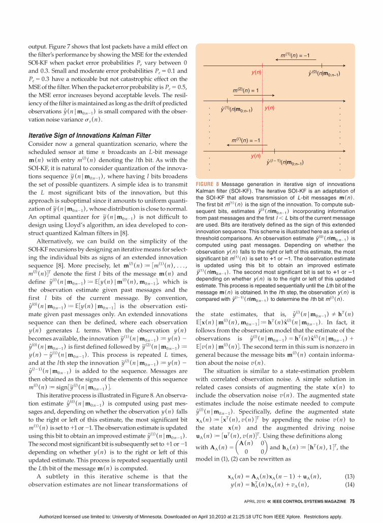
m(l) (n) J sign 3y|(l) (n|m0:n21 ) 4. This iterative process is illustrated in Figure 8. An observa-
tion estimate y(0) (n|m0:n21 ) is computed using past mes-
sages and, depending on whether the observation y (n) falls
to the right or left of this estimate, the most significant bit
m(1) (n) is set to 11 or 21. The observation estimate is updated
using this bit to obtain an improved estimate y(1) (n|m0:n21 ) .
The second most significant bit is subsequently set to 11 or 21
depending on whether y (n) is to the right or left of this
updated estimate. This process is repeated sequentially until
the Lth bit of the message m(n) is computed.
A subtlety in this iterative scheme is that the
observation estimates are not linear transformations of
the state estimates, that is, y(l) (n|m0:n21 ) 2 hT (n)
E 3x (n)|m(l) (n) , m0:n21 4 J hT (n) x(l) (n|m0:n21 ) . In fact, it
follows from the observation model that the estimate of the
observations is y(l) (n|m0:n21 ) 5 hT (n) x(l) (n|m0:n21 ) 1
E 3v (n)|m(l) (n) 4. The second term in this sum is nonzero in
general because the message bits m(l) (n) contain informa-
tion about the noise v (n) .
The situation is similar to a state-estimation problem
with correlated observation noise. A simple solution in
related cases consists of augmenting the state x (n) to
include the observation noise v (n) . The augmented state
estimates include the noise estimate needed to compute
y(l) (n|m0:n21 ) . Specifically, define the augmented state
xA(n) J 3xT (n) , v (n) 4T by appending the noise v (n) to
the state x (n) and the augmented driving noise
uA(n) J 3uT (n) , v (n)4T. Using these definitions along
with AA(n) 5 aA (n) 0
0 0b and hA(n) J 3hT (n) , 1 4T, the
model in (1), (2) can be rewritten as
xA(n) 5 AA(n)xA(n 2 1) 1 uA(n) , (13)
y (n) 5 hAT (n)xA(n) 1 vA(n) , (14)
y (n)
y (n)
y (n)
m (1)(n ) = −1
m (l )(n ) = −1
m (2)(n ) = 1
.
.
.
.
.
.
.
.
.
.
.
.
.
.
.
.
.
.
.
.
.
.
.
y (0)(n|m0:n−1)^
y (1)(n|m0:n−1)^
y (l – 1)(n|m0:n−1)^
FIGURE 8 Message generation in iterative sign of innovations
Kalman filter (SOI-KF). The iterative SOI-KF is an adaptation of
the SOI-KF that allows transmission of L-bit messages m(n ) .
The first bit m(1) (n ) is the sign of the innovation. To compute sub-
sequent bits, estimates y(l) (n|m0:n21) incorporating information
from past messages and the first l , L bits of the current message
are used. Bits are iteratively defined as the sign of this extended
innovation sequence. This scheme is illustrated here as a series of
threshold comparisons. An observation estimate y (0) (n|m0:n21) is
computed using past messages. Depending on whether the
observation y (n ) falls to the right or left of this estimate, the most
significant bit m(1) (n ) is set to 11 or 21. The observation estimate
is updated using this bit to obtain an improved estimate
y(1) (n|m0:n21) . The second most significant bit is set to 11 or 21
depending on whether y (n ) is to the right or left of this updated
estimate. This process is repeated sequentially until the Lth bit of the
message m(n ) is obtained. In the l th step, the observation y (n ) is
compared with y(l21) (n|m0:n21) to determine the l th bit m(l ) (n ) .
Authorized licensed use limited to: University of Minnesota. Downloaded on April 10,2010 at 21:25:18 UTC from IEEE Xplore. Restrictions apply.
76 IEEE CONTROL SYSTEMS MAGAZINE » APRIL 2010
where, by construction, the new observation noise vA(n) is
identically zero and thus can be thought of as normal noise
with variance svA
2 (n) 5 0. The correlation matrix of the
augmented driving noise is a block-diagonal matrix CuA(n) ,
with Cu (n) in the upper left corner and sv2 (n) in the lower
right one.
The augmented state formulation (13), (14) entails a state
with increased dimension but is otherwise equivalent to
(1), (2). However, the formulation has the appealing prop-
erty that MMSE estimates of the augmented state xA(n)
contain MMSE estimates of the original state x (n) and the
observation noise v (n) . As a result, y(l) (n|m0:n21 ) can be
obtained as a linear transformation of the augmented esti-
mates xA(l) (n|m0:n21 ) . Indeed, with vA(n) 5 0 it follows that
y(l) (n|m0:n21 ) 5 hAT (n) xA
(l) (n|m0:n21 ) .
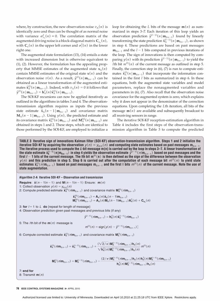
The SOI-KF recursions can now be applied iteratively as
outlined in the algorithms in tables 3 and 4. The observation-
transmission algorithm requires as inputs the previous
state estimate xA(n 2 1|m0:n21 ) and covariance matrix
MA(n 2 1|m0:n21 ) . Using y (n) , the predicted estimate and
its covariance matrix xA(0) (n|m0:n21 ) and MA
(0) (n|m0:n21 ) are
obtained in steps 1 and 2. These steps, which are identical to
those performed by the SOI-KF, are employed to initialize a
loop for obtaining the L bits of the message m(n) as sum-
marized in steps 3–7. Each iteration of this loop yields an
observation prediction y(l21) (n|m0:n21 ) found by linearly
transforming the state prediction xA(l21) (n|m0:n21 ) , as shown
in step 4. These predictions are based on past messages
m0:n21 and the l 2 1 bits computed in previous iterations of
the loop. The sign of innovations is then computed by com-
paring y (n) with its prediction y(l21) (n|m0:n21 ) to yield the
lth bit m(l) (n) of the current message as outlined in step 5.
Finally, the correction step in (6), (7) is run to compute esti-
mates xA(l) (n|m0:n21 ) that incorporate the information con-
tained in the first l bits as summarized in step 6. In these
equations, both the augmented state variables and model
parameters, replace the nonaugmented variables and
parameters in (6), (7). Also recall that the observation noise
covariance for the augmented system is zero, which explains
why it does not appear in the denominator of the correction
equations. Upon completing the Lth iteration, all bits of the
message m(n) are available and subsequently broadcast to
all receiving sensors in range.
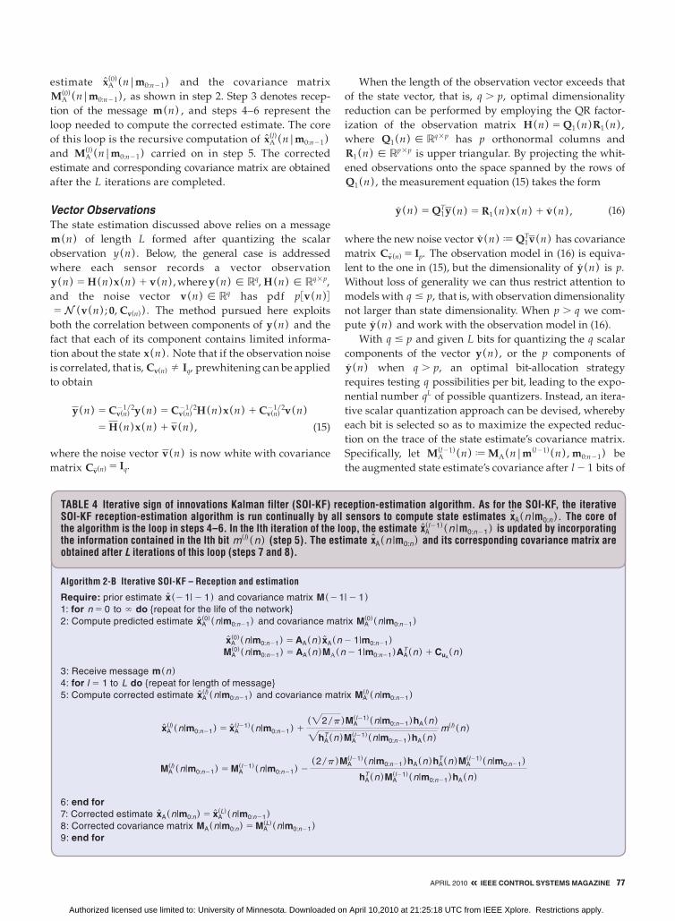
The iterative SOI-KF reception-estimation algorithm in
Table 4 includes the first steps of the observation-trans-
mission algorithm in Table 3 to compute the predicted
Algorithm 2-A Iterative SOI-KF – Observation and transmission
Require: x (n 2 1|n 2 1 ) and M(n 2 1|n 2 1 ) Ensure: m(n )
1: Collect observation y (n ) 5 yk(n) (n )
2: Compute predicted estimate xA(0) (n|m0:n21) and covariance matrix MA
(0) (n|m0:n21)
xA(0) (n|m0:n21) 5 AA(n ) xA(n 2 1|m0:n21)
MA(0) (n|m0:n21) 5 AA(n )MA(n 2 1|m0:n21)AA
T (n ) 1 CuA(n )
3: for l 5 1 to L do {repeat for length of message}
4: Observation prediction given past messages and previous bits (if any)
y(l21) (n|m0:n21) 5 hAT (n ) xA
(l21) (n|m0:n21)
5: The l th bit of the m(n ) message is
m(l) (n ) 5 sign 3y (n ) 2 y(l21) (n|m0:n21) 46: Compute corrected estimate xA
(l) (n|m0:n21) and covariance matrix MA(l) (n|m0:n21)
xA(l) (n|m0:n21) 5 xA
(l21) (n|m0:n21) 1("2/p )MA
(l21) (n|m0:n21)hA(n )
"hAT (n )MA
(l21) (n|m0:n21)hA(n ) m(l) (n )
MA(l) (n|m0:n21) 5 MA
(l21) (n|m0:n21) 2(2/p )MA
(l21) (n|m0:n21)hA(n )hAT (n )MA
(l21) (n|m0:n21)
hAT (n )MA
(l21) (n|m0:n21)hA(n )
7: end for 8: Transmit m(n )
TABLE 3 Iterative sign of innovations Kalman filter (SOI-KF) observation-transmission algorithm. Steps 1 and 2 initialize the iterative SOI-KF by acquiring the observation y (n) 5 yk(n) (n) and computing state estimates based on past messages m0:n21. The iterative process used to compute the L-bit message m(n) is carried out by the loop in steps 3–7. A linear transformation of the state estimate xA
(l21) (n |m0:n21 ) in step 4 yields the observation estimate y(l21) (n |m0:n21 ) based on past messages and the first l 2 1 bits of the current message. The lth bit m(l) (n ) is then defined as the sign of the difference between the observation y (n) and this prediction in step 5. Step 6 is carried out after the computation of each message bit m(l) (n) to yield state estimates xA
(l) (n |m0:n21 ) based on past messages m0:n21 and the first l bits m(l) (n) of the current message. Note the use of state augmentation.
Authorized licensed use limited to: University of Minnesota. Downloaded on April 10,2010 at 21:25:18 UTC from IEEE Xplore. Restrictions apply.
APRIL 2010 « IEEE CONTROL SYSTEMS MAGAZINE 77
estimate xA(0) (n|m0:n21 ) and the covariance matrix
MA(0) (n|m0:n21 ) , as shown in step 2. Step 3 denotes recep-
tion of the message m(n) , and steps 4–6 represent the
loop needed to compute the corrected estimate. The core
of this loop is the recursive computation of xA(l) (n|m0:n21 )
and MA(l) (n|m0:n21 ) carried on in step 5. The corrected
estimate and corresponding covariance matrix are obtained
after the L iterations are completed.
Vector Observations
The state estimation discussed above relies on a message
m(n) of length L formed after quantizing the scalar
observation y (n) . Below, the general case is addressed
where each sensor records a vector observation
y(n) 5 H(n)x (n) 1 v(n) , where y(n) [ Rq, H(n) [ Rq3p,
and the noise vector v(n) [ Rq has pdf p 3v(n)4 5N(v(n) ; 0, Cv(n) ) . The method pursued here exploits
both the correlation between components of y(n) and the
fact that each of its component contains limited informa-
tion about the state x (n) . Note that if the observation noise
is correlated, that is, Cv(n) 2 Iq, prewhitening can be applied
to obtain
y(n) 5 Cv(n)21/2y(n) 5 Cv(n)
21/2H(n)x (n) 1 Cv(n)21/2v(n)
5 H(n)x (n) 1 v(n) , (15)
where the noise vector v(n) is now white with covariance
matrix Cv(n) 5 Iq.
When the length of the observation vector exceeds that
of the state vector, that is, q . p, optimal dimensionality
reduction can be performed by employing the QR factor-
ization of the observation matrix H(n) 5 Q1 (n)R1 (n) ,
where Q1 (n) [ Rq3p has p orthonormal columns and
R1 (n) [ Rp3p is upper triangular. By projecting the whit-
ened observations onto the space spanned by the rows of
Q1 (n) , the measurement equation (15) takes the form
y?
(n) 5 Q1Ty(n) 5 R1 (n)x (n) 1 v
?
(n) , (16)
where the new noise vector v?
(n) J Q1Tv(n) has covariance
matrix Cv?
(n) 5 Ip. The observation model in (16) is equiva-
lent to the one in (15), but the dimensionality of y?
(n) is p.
Without loss of generality we can thus restrict attention to
models with q # p, that is, with observation dimensionality
not larger than state dimensionality. When p . q we com-
pute y?
(n) and work with the observation model in (16).
With q # p and given L bits for quantizing the q scalar
components of the vector y(n) , or the p components of
y?
(n) when q . p, an optimal bit-allocation strategy
requires testing q possibilities per bit, leading to the expo-
nential number qL of possible quantizers. Instead, an itera-
tive scalar quantization approach can be devised, whereby
each bit is selected so as to maximize the expected reduc-
tion on the trace of the state estimate’s covariance matrix.
Specifically, let MA(l21) (n) J MA(n|m(l21) (n) , m0:n21 ) be
the augmented state estimate’s covariance after l 2 1 bits of
Algorithm 2-B Iterative SOI-KF – Reception and estimation
Require: prior estimate x (2 1| 2 1 ) and covariance matrix M(2 1| 2 1 )
1: for n 5 0 to ` do {repeat for the life of the network}
2: Compute predicted estimate xA(0) (n|m0:n21) and covariance matrix MA
(0) (n|m0:n21)
xA(0) (n|m0:n21) 5 AA(n ) xA(n 2 1|m0:n21)
MA(0) (n|m0:n21) 5 AA(n )MA(n 2 1|m0:n21)AA
T (n ) 1 CuA(n )
3: Receive message m(n )
4: for l 5 1 to L do {repeat for length of message}
5: Compute corrected estimate xA(l) (n|m0:n21) and covariance matrix MA
(l) (n|m0:n21)
xA(l) (n|m0:n21) 5 xA
(l21) (n|m0:n21) 1("2/p )MA
(l21) (n|m0:n21)hA(n )
"hAT (n )MA
(l21) (n|m0:n21)hA(n ) m(l) (n )
MA(l) (n|m0:n21) 5 MA
(l21) (n|m0:n21) 2(2/p )MA
(l21) (n|m0:n21)hA(n )hAT (n )MA
(l21) (n|m0:n21)
hAT (n )MA
(l21) (n|m0:n21)hA(n )
6: end for 7: Corrected estimate xA(n|m0:n) 5 xA
(L) (n|m0:n21)
8: Corrected covariance matrix MA(n|m0:n) 5 MA(L) (n|m0:n21)
9: end for
TABLE 4 Iterative sign of innovations Kalman filter (SOI-KF) reception-estimation algorithm. As for the SOI-KF, the iterative SOI-KF reception-estimation algorithm is run continually by all sensors to compute state estimates xA (n |m0:n ) . The core of the algorithm is the loop in steps 4–6. In the lth iteration of the loop, the estimate xA
(l21) (n |m0:n21 ) is updated by incorporating the information contained in the Ith bit m(l) (n) (step 5). The estimate xA (n |m0:n ) and its corresponding covariance matrix are obtained after L iterations of this loop (steps 7 and 8).
Authorized licensed use limited to: University of Minnesota. Downloaded on April 10,2010 at 21:25:18 UTC from IEEE Xplore. Restrictions apply.
78 IEEE CONTROL SYSTEMS MAGAZINE » APRIL 2010
the message m(n) are utilized in the iterative SOI-KF cor-
rections and consider the augmented measurement matrix
HA(n) J 3H(n) Iq 4 of the whitened observation model in
(15); when q . p, consider the reduced-dimensionality
model in (16) and redefine HA(n) J 3R1 (n) Iq 4. The lth bit
is allocated to quantize the jth entry y (n, j ) of the obser-
vation y(n) if the corresponding row vector hAT (n, j ) of
the augmented measurement matrix HA(n) maximizes
the quantity
tra 2
p 3MA
(l21) (n)hA(n, j )hAT (n, j )MA
(l21) (n) 41:p, 1:p
hAT (n, j )MA
(l21) (n)hA(n, j )b
52
p 7 3MA
(l21) (n)hA(n, j ) 41:p 7 2hA
T (n, j )MA(l21) (n)hA(n, j )
, (17)
among all j 5 1, c, q. This process requires evaluating
Lq terms of the form (17) to determine all of the bits of the
message m(n) .
Experimental Results
The iterative extended SOI-KF algorithm is tested experi-
mentally and compared to the extended Kalman filter
based on nonquantized amplitude observations. The appli-
cation involves autonomous underwater vehicles perform-
ing cooperative multirobot localization [13], [14]. The state
vector to be estimated is x 5 3x1, y1, n1, f1, x2 , y2 , n2 , f2 4T,
where xi, yi denote the position coordinates of robot i, ni
is the horizontal velocity, and fi is the heading direction
(yaw), for i 5 1, 2. A zero-acceleration model is used to describe
the nonholonomic motion of each vehicle with xi(n11)5 xi(n)
1 ni ( n) Ts cosfi ( n), yi(n 11) 5 yi (n) 1ni (n)Ts sinfi(n) ,
ni(n 1 1) 5 ni(n) 1 u .ni
(n)Ts, fi(n 1 1) 5 fi(n) 1 u .fi
(n)Ts,
where Ts 5 0.05 s is the sampling period,uni# (n),N(un
i
# (n) ;
0, sni
#2 ) , and uf#i(n) ,N(uf
#i(n) ; 0, sfi
#2 ) , with sv#15 sv
#2
5 0.28 m/s2, sf#
15 sf
#25 8.3 deg/s.
The yaw fi, pitch ci, and roll zi, of robot i are measured
by an onboard MicroStrain 3DM-GX1 AHRS inertial sensor.
The noise in these measurements is modeled as zero-mean
normal with standard deviations sfi5 sci
5 szi5 2°,
i 5 1, 2. The yaw measurement yfi(n) 5 fi(n) 1 vfi
(n) ,
vfi(n) ,N(vfi
(n) ; 0, sfi
2 ) is processed by the filter to pro-
vide corrections for the estimates of the heading direction of
the vehicle. The pitch measurement cmi(n) 5 ci(n)
1 vci(n) , vci
(n) ,N(vci(n) ; 0, svci
2 ) is combined with the
measurement nmir 5 nir (n) 1 vnir, vnir(n) ,N(vnir
(n) ; 0, svnir
2 ) ,
svnir5 0.25 m/s, of the vehicles’ longitudinal velocity for
constructing a measurement of its horizontal velocity
yni(n) 5 nmir (n)coscmi(n) . ni(n) 1 vni
(n) , i 5 1, 2. To ob-
tain this approximation for yni(n) , a first-order Taylor
series approximation is applied, and the noise vni(n) .
nmir (n)sincmi(n)vci(n) 2 coscmi(n)vnir
(n) is approximated
as zero-mean normal with variance svni
2 (n) 5
(nmir (n) ) 2sin2 cmi(n)sci
2 1 cos2 cmi(n)snir2 . The longitudinal
velocity measurement nmir is inferred from measurements
of the propeller’s rate of rotation using a linear approxima-
tion [14].
The autonomous underwater vehicles are equipped
with acoustic modems for underwater communication and
for calculating the range to the transmitting robot using the
time of flight and speed of sound in water ( 1500 m/s). The
distance measurement between the two vehicles is
ydij(n) 5!(xi(n)2xj(n)) 2 1 (yi(n) 2 yj(n)) 21vdij
(n), where
vdij(n) ,N(vdij
(n) ; 0, sdij
2 ) and sdij5 10 m.
The duration of the experiment is about 15 min, during
which time the two autonomous underwater vehicles cover
distances of 1.16 km and 1.18 km, respectively. Two sce-
narios are examined. In the first one, the robots communi-
cate to each other their nonquantized amplitude
measurements of velocity and heading along with the
24 distance measurements recorded during this experi-
ment; see Figure 9. These measurements are processed
locally on each vehicle by an extended Kalman filter to
jointly estimate both trajectories. In the second scenario,
only 3 bits per scalar measurement are communicated
between the two autonomous vehicles, and the iterative
extended SOI-KF is used for processing them. As shown in
figures 10 and 11, the iterative extended SOI-KF is able to
approximate the robots’ trajectories estimated by the
extended Kalman filter, while using only 3 bits per obser-
vation. The root mean squared differences between the
extended Kalman filter and iterative extended SOI-KF
estimates for the x and y coordinates of the two robots are
(2.78 m, 2.95 m) and (1.55 m, 5.35 m), respectively, all
of which are less than 0.5% of the distance traveled by
each robot.
CONSENSUS-BASED DISTRIBUTED KALMAN FILTERING AND SMOOTHINGWe now assume that sensors can exchange information only
with neighboring sensors located within a predefined trans-
mission radius. The challenge is to obtain the quantities
needed to perform MMSE estimation with manageable com-
munication cost. Toward this end, sensors can exchange mes-
sages with their neighbors to estimate quantities that are
essential for implementing the centralized Kalman filter
recursions. To compute these quantities, sensors use recur-
sive data aggregation schemes to combine their local infor-
mation with messages they receive from their neighbors.
Since the information gathered at different sensors is corre-
lated, these recursive schemes reduce the communication
cost of the distributed state-estimation algorithms [15]–[19].
Instrumental for implementing distributed Kalman
filter approaches is the notion of consensus averaging,
which performs distributed computation of sample aver-
ages across sensors. In consensus averaging, each sensor
maintains a local state variable that provides an estimate of
the desired sample average and performs two steps to
update these local state variables. In the first step, each
Authorized licensed use limited to: University of Minnesota. Downloaded on April 10,2010 at 21:25:18 UTC from IEEE Xplore. Restrictions apply.
APRIL 2010 « IEEE CONTROL SYSTEMS MAGAZINE 79
sensor transmits its estimate to neighboring sensors and
receives, in return, the neighboring sensors’ local esti-
mates. In the second step, each sensor updates its state by
forming a weighted sum of its own and neighboring esti-
mates. Upon selecting suitable weights to form these up-
dates and assuming ideal inter-sensor communications,
the sensor estimates converge to the desired sample aver-
age as the number of updates grows large [20]–[22].
Consensus-averaging schemes perform poorly in the
presence of noise in the intersensor links, to the extent that
they diverge [23]. However, algorithms based on consensus
averaging that are robust against noise perturbations for
distributed estimation are available [24]. Consensus-aver-
aging schemes can also be utilized to distribute the central-
ized Kalman filter recursions. The prediction recursions are
identical to (4)–(5). Using the information form of the Kalman
filter [25, p. 139], however, the corrected state and corre-
sponding corrected error covariance matrix are given by
M (n|n) J M (n|y0:n ) 5 3I(n) 1 M21 (n|n 2 1) 421,
(18)
x (n|n) J x (n|y0:n ) 5 x (n|n 2 1)
1 M (n|n) 3c (n) 2I(n) x (n|n2 1)4, (19)
where
I(n) J aK
k51
svk
22 (n)hk(n)hkT (n) ,
c (n) J aK
k51
svk
22 (n)hk(n)yk(n) . (20)
If sensors have available local estimates xk(n 2 1|n 2 1) and
the corresponding Mk(n 2 1|n 2 1) , then each sensor could
run the prediction recursions in (4)–(5) in a distributed fashion
provided that the model parameters A (n) and Cu (n) are
known at each sensor. However, (18) and (19) require I(n)
and c (n) to be acquired at each sensor. This acquisition can be
carried out using consensus averaging because I(n) and
c (n) are averages with the kth summand located at sensor k.
Existing distributed Kalman filter approaches rely
on consensus-based algorithms to form estimates
Ik(n; n : n 1 N ) and ck(n; n :n 1 N ) through N 1 1 recur-
sions starting at n and finishing at n 1 N [15], [17]. When
these estimates are plugged into (18) and (19), local esti-
mates xk(n|n; n :n 1 N ) for the state x (n) using observa-
tions up to time n necessitate consensus iterations
performed between times n and n 1 N as signified by the
−150 −100 −50 0 50 100
20
40
60
80
100
120
140
160
180
200
220
x (m)
y (m
)
Robot 1 Robot 2
Distance Measurement
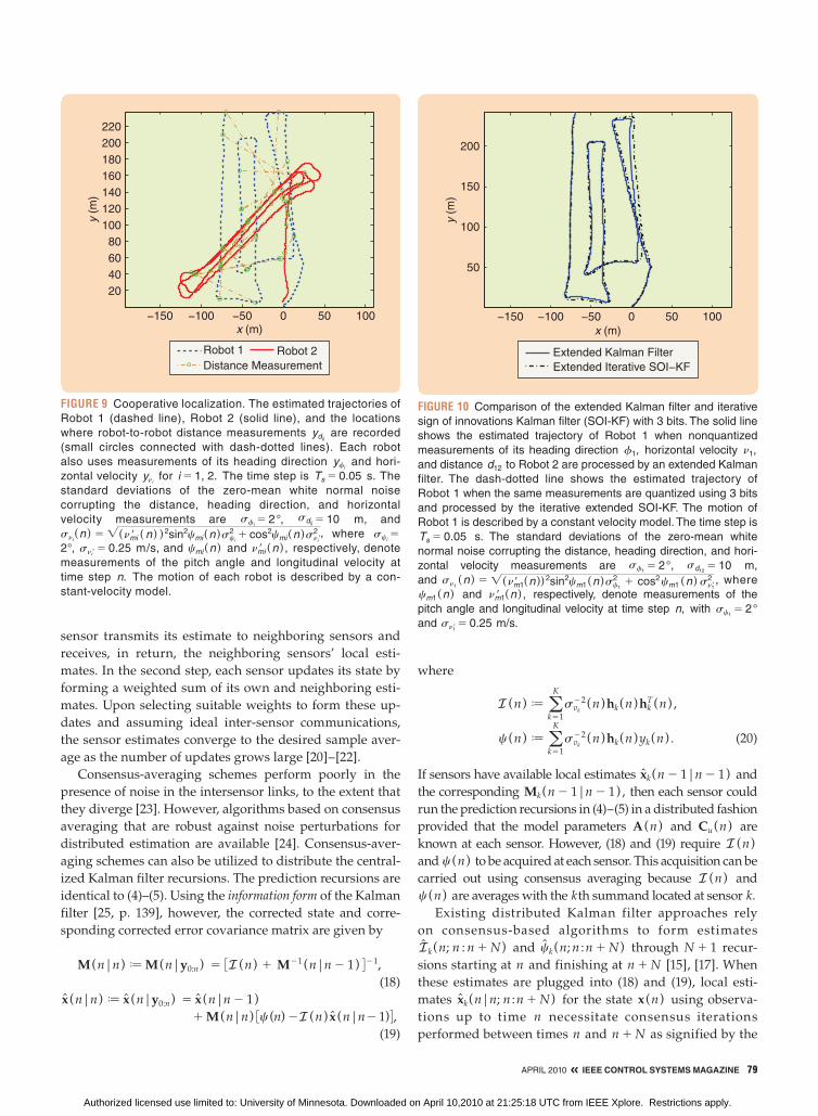
FIGURE 9 Cooperative localization. The estimated trajectories of
Robot 1 (dashed line), Robot 2 (solid line), and the locations
where robot-to-robot distance measurements ydij are recorded
(small circles connected with dash-dotted lines). Each robot
also uses measurements of its heading direction yfi and hori-
zontal velocity yni for i 5 1, 2. The time step is Ts 5 0.05 s. The
standard deviations of the zero-mean white normal noise
corrupting the distance, heading direction, and horizontal
velocity measurements are sfi5 2°, sdij 5 10 m, and
sni(n ) 5 ! (nmir ( n ) )2sin2cmi(n )sci
2 1 cos2cmi(n )snir2 , where sci
5
2°, snir 5 0.25 m/s, and cmi(n ) and nmir (n ) , respectively, denote
measurements of the pitch angle and longitudinal velocity at
time step n. The motion of each robot is described by a con-
stant-velocity model.
−150 −100 −50 0 50 100
50
100
150
200
x (m)
y (m
)
Extended Kalman Filter
Extended Iterative SOI−KF
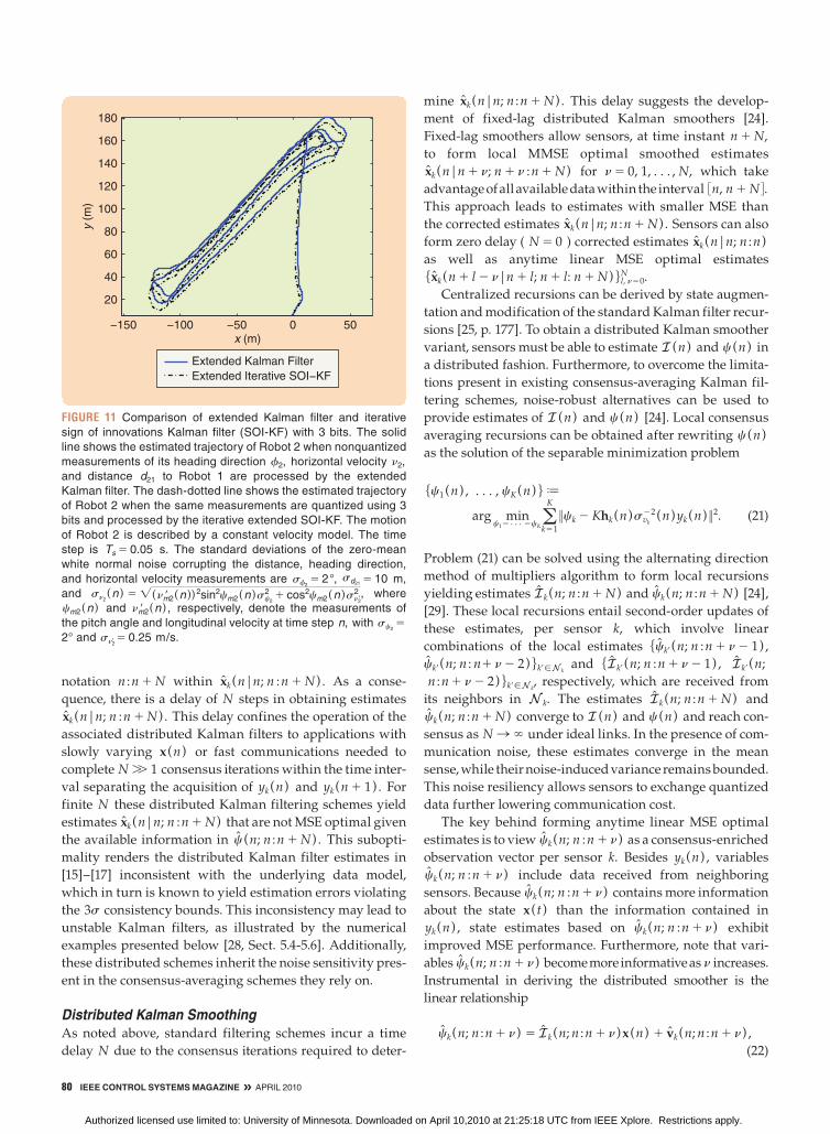
FIGURE 10 Comparison of the extended Kalman filter and iterative
sign of innovations Kalman filter (SOI-KF) with 3 bits. The solid line
shows the estimated trajectory of Robot 1 when nonquantized
measurements of its heading direction f1, horizontal velocity n1,
and distance d12 to Robot 2 are processed by an extended Kalman
filter. The dash-dotted line shows the estimated trajectory of
Robot 1 when the same measurements are quantized using 3 bits
and processed by the iterative extended SOI-KF. The motion of
Robot 1 is described by a constant velocity model. The time step is
Ts 5 0.05 s. The standard deviations of the zero-mean white
normal noise corrupting the distance, heading direction, and hori-
zontal velocity measurements are sf15 2°, sd12
5 10 m,
and sn1(n ) 5 ! (nm1r (n ))2sin2cm1(n )sc1
2 1 cos2 cm1 (n ) sn1r2 , where
cm1(n ) and nm1r (n ) , respectively, denote measurements of the
pitch angle and longitudinal velocity at time step n, with sc15 2°
and sn1r 5 0.25 m/s.
Authorized licensed use limited to: University of Minnesota. Downloaded on April 10,2010 at 21:25:18 UTC from IEEE Xplore. Restrictions apply.
80 IEEE CONTROL SYSTEMS MAGAZINE » APRIL 2010
notation n :n 1 N within xk(n|n; n :n 1 N ) . As a conse-
quence, there is a delay of N steps in obtaining estimates
xk(n|n; n :n 1 N ) . This delay confines the operation of the
associated distributed Kalman filters to applications with
slowly varying x (n) or fast communications needed to
complete N W 1 consensus iterations within the time inter-
val separating the acquisition of yk(n) and yk(n 1 1) . For
finite N these distributed Kalman filtering schemes yield
estimates xk(n|n; n :n 1 N ) that are not MSE optimal given
the available information in c (n; n :n 1 N ) . This subopti-
mality renders the distributed Kalman filter estimates in
[15]–[17] inconsistent with the underlying data model,
which in turn is known to yield estimation errors violating
the 3s consistency bounds. This inconsistency may lead to
unstable Kalman filters, as illustrated by the numerical
examples presented below [28, Sect. 5.4-5.6]. Additionally,
these distributed schemes inherit the noise sensitivity pres-
ent in the consensus-averaging schemes they rely on.
Distributed Kalman Smoothing
As noted above, standard filtering schemes incur a time
delay N due to the consensus iterations required to deter-
mine xk(n|n; n :n 1 N ) . This delay suggests the develop-
ment of fixed-lag distributed Kalman smoothers [24].
Fixed-lag smoothers allow sensors, at time instant n 1 N,
to form local MMSE optimal smoothed estimates
xk(n|n 1 n; n 1 n :n 1 N ) for n 5 0, 1, c, N, which take
advantage of all available data within the interval 3n, n 1 N 4. This approach leads to estimates with smaller MSE than
the corrected estimates xk(n|n; n :n 1 N ) . Sensors can also
form zero delay ( N 5 0 ) corrected estimates xk(n|n; n :n)
as well as anytime linear MSE optimal estimates
5xk(n 1 l 2 n|n 1 l; n 1 l: n 1 N ) 6l, n50N .
Centralized recursions can be derived by state augmen-
tation and modification of the standard Kalman filter recur-
sions [25, p. 177]. To obtain a distributed Kalman smoother
variant, sensors must be able to estimate I(n) and c (n) in
a distributed fashion. Furthermore, to overcome the limita-
tions present in existing consensus- averaging Kalman fil-
tering schemes, noise-robust alternatives can be used to
provide estimates of I(n) and c (n) [24]. Local consensus
averaging recursions can be obtained after rewriting c (n)
as the solution of the separable minimization problem
5c1 (n) , c, cK (n) 6 J
arg minc15c5cK
aK
k51
7ck 2 Khk(n)svk
22 (n)yk(n) 7 2. (21)
Problem (21) can be solved using the alternating direction
method of multipliers algorithm to form local recursions
yielding estimates Ik(n; n :n 1 N ) and ck(n; n :n 1 N ) [24],
[29]. These local recursions entail second-order updates of
these estimates, per sensor k, which involve linear
combinations of the local estimates 5ckr (n; n :n 1 n 2 1) ,
ckr (n; n : n1 n 2 2) 6kr[Nk and 5Ikr (n; n :n 1 n 2 1) , Ikr (n;
n :n 1 n 2 2) 6kr[Nk, respectively, which are received from
its neighbors in Nk. The estimates Ik(n; n :n 1 N ) and
ck(n; n :n 1 N ) converge to I(n) and c (n) and reach con-
sensus as N S ` under ideal links. In the presence of com-
munication noise, these estimates converge in the mean
sense, while their noise-induced variance remains bounded.
This noise resiliency allows sensors to exchange quantized
data further lowering communication cost.
The key behind forming anytime linear MSE optimal
estimates is to view ck(n; n :n 1 n ) as a consensus-enriched
observation vector per sensor k. Besides yk(n) , variables
ck(n; n :n 1 n ) include data received from neighboring
sensors. Because ck(n; n :n 1 n ) contains more information
about the state x ( t ) than the information contained in
yk(n) , state estimates based on ck(n; n :n 1 n ) exhibit
improved MSE performance. Furthermore, note that vari-
ables ck(n; n :n 1 n ) become more informative as n increases.
Instrumental in deriving the distributed smoother is the
linear relationship
ck(n; n :n 1 n ) 5 Ik(n; n :n 1 n )x (n) 1 vk(n; n :n 1 n ) ,
(22)
−150 −100 −50 0 50
20
40
60
80
100
120
140
160
180
x (m)
y (m
)
Extended Kalman Filter
Extended Iterative SOI−KF
FIGURE 11 Comparison of extended Kalman filter and iterative
sign of innovations Kalman filter (SOI-KF) with 3 bits. The solid
line shows the estimated trajectory of Robot 2 when nonquantized
measurements of its heading direction f2, horizontal velocity n2,
and distance d21 to Robot 1 are processed by the extended
Kalman filter. The dash-dotted line shows the estimated trajectory
of Robot 2 when the same measurements are quantized using 3
bits and processed by the iterative extended SOI-KF. The motion
of Robot 2 is described by a constant velocity model. The time
step is Ts 5 0.05 s. The standard deviations of the zero-mean
white normal noise corrupting the distance, heading direction,
and horizontal velocity measurements are sf25 2°, sd21
5 10 m,
and sn2(n ) 5 ! (nm2r (n ))2sin2cm2(n )sc2
2 1 cos2cm2(n )sn2r2 , where
cm2(n ) and nm2r (n ) , respectively, denote the measurements of
the pitch angle and longitudinal velocity at time step n, with sc25
2° and sn2r 5 0.25 m/s.
Authorized licensed use limited to: University of Minnesota. Downloaded on April 10,2010 at 21:25:18 UTC from IEEE Xplore. Restrictions apply.
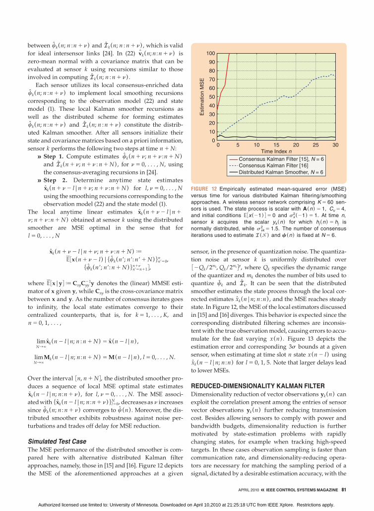
APRIL 2010 « IEEE CONTROL SYSTEMS MAGAZINE 81
between ck(n; n :n 1 n ) and Ik(n; n : n 1 n ) , which is valid
for ideal intersensor links [24]. In (22) vk(n; n :n 1 n ) is
zero-mean normal with a covariance matrix that can be
evaluated at sensor k using recursions similar to those
involved in computing Ik(n; n : n 1 n ) .
Each sensor utilizes its local consensus-enriched data
ck(n; n :n 1 n ) to implement local smoothing recursions
corresponding to the observation model (22) and state
model (1). These local Kalman smoother recursions as
well as the distributed scheme for forming estimates
ck(n; n :n 1 n ) and Ik(n; n : n 1 n ) constitute the distrib-
uted Kalman smoother. After all sensors initialize their
state and covariance matrices based on a priori information,
sensor k performs the following two steps at time n 1 N:
Step 1. » Compute estimates ck(n 1 n; n 1 n :n 1 N )
and Ik(n 1 n; n 1 n : n 1 N ) , for n 5 0, c, N, using
the consensus-averaging recursions in [24].
Step 2. » Determine anytime state estimates
xk(n 1 n 2 l|n 1 n; n 1 n :n 1 N ) for l, n 5 0, c, N
using the smoothing recursions corresponding to the
observation model (22) and the state model (1).
The local anytime linear estimates xk(n 1 n 2 l|n 1
n; n 1 n :n 1 N ) obtained at sensor k using the distributed
smoother are MSE optimal in the sense that for
l 5 0, c, N
xk(n 1 n 2 l|n 1 n; n 1 n :n 1 N ) J
E 3x (n 1 n 2 l)|5ck(n r; n r: n r1 N ) 6nr50n ,
5ck(n r; n r: n 1 N ) 6nr5n11n1n 4,
where E 3x|y 4 J CxyCyy21y denotes the (linear) MMSE esti-
mator of x given y, while Cxy is the cross-covariance matrix
between x and y. As the number of consensus iterates goes
to infinity, the local state estimates converge to their
centralized counterparts, that is, for k 5 1, c, K, and
n 5 0, 1, c,
limNS`
xk(n 2 l|n; n : n 1 N ) 5 x (n 2 l|n) ,
limNS`
Mk(n 2 l|n; n :n 1 N ) 5 M (n 2 l|n) , l 5 0, c, N.
Over the interval 3n, n 1 N 4, the distributed smoother pro-
duces a sequence of local MSE optimal state estimates
xk(n 2 l|n; n:n 1 n ) , for l, n 5 0, c, N. The MSE associ-
ated with 5xk(n 2 l|n; n :n 1 n ) 6l50N , decreases as n increases
since ck(n; n : n 1 n ) converges to c (n) . Moreover, the dis-
tributed smoother exhibits robustness against noise per-
turbations and trades off delay for MSE reduction.
Simulated Test Case
The MSE performance of the distributed smoother is com-
pared here with alternative distributed Kalman filter
approaches, namely, those in [15] and [16]. Figure 12 depicts
the MSE of the aforementioned approaches at a given
sensor, in the presence of quantization noise. The quantiza-
tion noise at sensor k is uniformly distributed over
32Qk/2mk, Qk/2mk 4p, where Qk specifies the dynamic range
of the quantizer and mk denotes the number of bits used to
quantize ck and Ik. It can be seen that the distributed
smoother estimates the state process through the local cor-
rected estimates xk(n|n; n :n) , and the MSE reaches steady
state. In Figure 12, the MSE of the local estimators discussed
in [15] and [16] diverges. This behavior is expected since the
corresponding distributed filtering schemes are inconsis-
tent with the true observation model, causing errors to accu-
mulate for the fast varying x (n) . Figure 13 depicts the
estimation error and corresponding 3s bounds at a given
sensor, when estimating at time slot n state x (n 2 l) using
xk(n 2 l|n; n :n) for l 5 0, 1, 5. Note that larger delays lead
to lower MSEs.
REDUCED-DIMENSIONALITY KALMAN FILTERDimensionality reduction of vector observations yk(n) can
exploit the correlation present among the entries of sensor
vector observations yk(n) further reducing transmission
cost. Besides allowing sensors to comply with power and
bandwidth budgets, dimensionality reduction is further
motivated by state-estimation problems with rapidly
changing states, for example when tracking high-speed
targets. In these cases observation sampling is faster than
communication rate, and dimensionality-reducing opera-
tors are necessary for matching the sampling period of a
signal, dictated by a desirable estimation accuracy, with the
0 5 10 15 20 25 300
10
20
30
40
50
60
70
80
90
100
Time Index n
Estim
ation M
SE
Consensus Kalman Filter [15], N = 6
Consensus Kalman Filter [16]
Distributed Kalman Smoother, N = 6
FIGURE 12 Empirically estimated mean-squared error (MSE)
versus time for various distributed Kalman filtering/smoothing
approaches. A wireless sensor network comprising K 5 60 sen-
sors is used. The state process is scalar with A(n ) 5 1, Cu 5 4,
and initial conditions E 3x (21 ) 4 5 0 and sx2(21 ) 5 1. At time n,
sensor k acquires the scalar yk (n ) for which hj(n ) 5 hj is
normally distributed, while svk2 5 1.5. The number of consensus
iterations used to estimate I (n ) and c (n ) is fixed at N 5 6.
Authorized licensed use limited to: University of Minnesota. Downloaded on April 10,2010 at 21:25:18 UTC from IEEE Xplore. Restrictions apply.
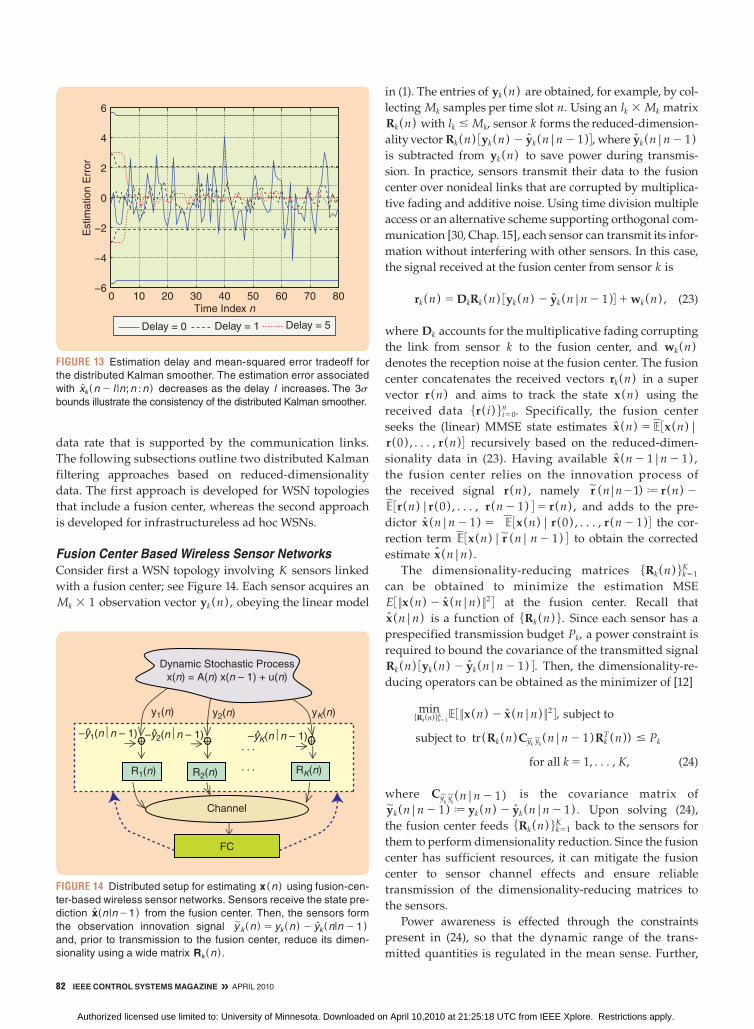
82 IEEE CONTROL SYSTEMS MAGAZINE » APRIL 2010
data rate that is supported by the communication links.
The following subsections outline two distributed Kalman
filtering approaches based on reduced-dimensionality
data. The first approach is developed for WSN topologies
that include a fusion center, whereas the second approach
is developed for infrastructureless ad hoc WSNs.
Fusion Center Based Wireless Sensor Networks
Consider first a WSN topology involving K sensors linked
with a fusion center; see Figure 14. Each sensor acquires an
Mk 3 1 observation vector yk(n) , obeying the linear model
in (1). The entries of yk(n) are obtained, for example, by col-
lecting Mk samples per time slot n. Using an lk 3 Mk matrix
Rk(n) with lk # Mk, sensor k forms the reduced-dimension-
ality vector Rk(n) 3yk(n) 2 yk(n|n 2 1)4, where yk(n|n 2 1)
is subtracted from yk(n) to save power during transmis-
sion. In practice, sensors transmit their data to the fusion
center over nonideal links that are corrupted by multiplica-
tive fading and additive noise. Using time division multiple
access or an alternative scheme supporting orthogonal com-
munication [30, Chap. 15], each sensor can transmit its infor-
mation without interfering with other sensors. In this case,
the signal received at the fusion center from sensor k is
rk(n) 5 DkRk(n) 3yk(n) 2 yk(n|n 2 1)41 wk(n) , (23)
where Dk accounts for the multiplicative fading corrupting
the link from sensor k to the fusion center, and wk(n)
denotes the reception noise at the fusion center. The fusion
center concatenates the received vectors rk(n) in a super
vector r (n) and aims to track the state x (n) using the
received data 5r ( i) 6i50n . Specifically, the fusion center
seeks the (linear) MMSE state estimates x (n) 5 E 3x (n)|
r (0) , c, r (n)4 recursively based on the reduced-dimen-
sionality data in (23). Having available x (n 2 1|n 2 1) ,
the fusion center relies on the innovation process of
the received signal r (n) , namely r| (n|n21) J r (n) 2
E 3r (n)|r (0) ,c, r (n 2 1) 45 r (n) , and adds to the pre-
dictor x (n|n 2 1) 5 E 3x (n)| r (0) , c, r (n 2 1)4 the cor-
rection term E 3x (n)| r| (n| n 2 1) 4 to obtain the corrected
estimate x (n|n) .
The dimensionality-reducing matrices 5Rk(n) 6k51K
can be obtained to minimize the estimation MSE
E 3 7x (n) 2 x (n|n) 7 2 4 at the fusion center. Recall that
x (n|n) is a function of 5Rk(n) 6. Since each sensor has a
prespecified transmission budget Pk, a power constraint is
required to bound the covariance of the transmitted signal
Rk(n) 3yk(n) 2 yk(n|n 2 1) 4. Then, the dimensionality-re-
ducing operators can be obtained as the minimizer of [12]
min5Rk(n)6k51K E 3 7x (n) 2 x (n|n) 7 2 4, subject to
subject to tr(Rk(n)Cy,k y,k(n|n 2 1)Rk
T (n)) # Pk
for all k 5 1, c, K, (24)
where Cy,k
y,k(n|n 2 1) is the covariance matrix of
y|k(n|n 2 1) J yk(n) 2 yk(n|n 2 1) . Upon solving (24),
the fusion center feeds 5Rk(n) 6k51K back to the sensors for
them to perform dimensionality reduction. Since the fusion
center has sufficient resources, it can mitigate the fusion
center to sensor channel effects and ensure reliable
transmission of the dimensionality-reducing matrices to
the sensors.
Power awareness is effected through the constraints
present in (24), so that the dynamic range of the trans-
mitted quantities is regulated in the mean sense. Further,
0 10 20 30 40 50 60 70 80−6
−4
−2
0
2
4
6
Time Index n
Estim
ation E
rror
Delay = 5Delay = 1Delay = 0
FIGURE 13 Estimation delay and mean-squared error tradeoff for
the distributed Kalman smoother. The estimation error associated
with xk (n 2 l |n;n :n ) decreases as the delay l increases. The 3s
bounds illustrate the consistency of the distributed Kalman smoother.
y1(n)
R1(n) R2(n) RK(n)
y2(n) yK(n)
–y1(n⏐n – 1)^ –y2(n⏐n – 1)^ –yK(n⏐n – 1)^
Channel
FC
. . .
. . .
Dynamic Stochastic Process
x(n) = A(n) x(n – 1) + u(n)
FIGURE 14 Distributed setup for estimating x (n ) using fusion-cen-
ter-based wireless sensor networks. Sensors receive the state pre-
diction x(n|n 21 ) from the fusion center. Then, the sensors form
the observation innovation signal y|k (n ) 5 yk (n ) 2 yk (n|n 2 1 )
and, prior to transmission to the fusion center, reduce its dimen-
sionality using a wide matrix Rk (n ) .
Authorized licensed use limited to: University of Minnesota. Downloaded on April 10,2010 at 21:25:18 UTC from IEEE Xplore. Restrictions apply.
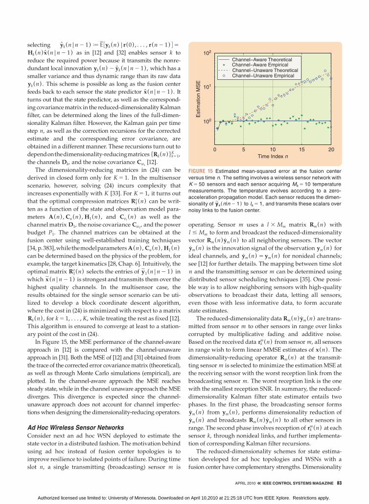
APRIL 2010 « IEEE CONTROL SYSTEMS MAGAZINE 83
selecting yk(n|n 2 1) J E 3yk(n)|r (0) , c, r (n 2 1) 45
Hk(n) x (n|n 2 1) as in [12] and [32] enables sensor k to
reduce the required power because it transmits the nonre-
dundant local innovation yk(n) 2 yk(n|n 2 1) , which has a
smaller variance and thus dynamic range than its raw data
yk(n) . This scheme is possible as long as the fusion center
feeds back to each sensor the state predictor x (n|n 2 1) . It
turns out that the state predictor, as well as the correspond-
ing covariance matrix in the reduced-dimensionality Kalman
filter, can be determined along the lines of the full-dimen-
sionality Kalman filter. However, the Kalman gain per time
step n, as well as the correction recursions for the corrected
estimate and the corresponding error covariance, are
obtained in a different manner. These recursions turn out to
depend on the dimensionality-reducing matrices 5Rk(n) 6k51K ,
the channels Dk, and the noise covariance Cwk [12].
The dimensionality-reducing matrices in (24) can be
derived in closed form only for K 5 1. In the multisensor
scenario, however, solving (24) incurs complexity that
increases exponentially with K [33]. For K 5 1, it turns out
that the optimal compression matrices R1o (n) can be writ-
ten as a function of the state and observation model para-
meters A (n) , Cu (n) , H1 (n) , and Cv1(n) as well as the
channel matrix D1, the noise covariance Cw1, and the power
budget P1. The channel matrices can be obtained at the
fusion center using well-established training techniques
[34, p. 383], while the model parameters A (n) , Cu (n) , H1 (n)
can be determined based on the physics of the problem, for
example, the target kinematics [28, Chap. 6]. Intuitively, the
optimal matrix R1o (n) selects the entries of y|1 (n|n 2 1) in
which x| (n|n 2 1) is strongest and transmits them over the
highest quality channels. In the multisensor case, the
results obtained for the single sensor scenario can be uti-
lized to develop a block coordinate descent algorithm,
where the cost in (24) is minimized with respect to a matrix
Rk(n) , for k 5 1, c, K, while treating the rest as fixed [12].
This algorithm is ensured to converge at least to a station-
ary point of the cost in (24).
In Figure 15, the MSE performance of the channel-aware
approach in [12] is compared with the channel-unaware
approach in [31]. Both the MSE of [12] and [31] obtained from
the trace of the corrected error covariance matrix (theoretical),
as well as through Monte Carlo simulations (empirical), are
plotted. In the channel-aware approach the MSE reaches
steady state, while in the channel unaware approach the MSE
diverges. This divergence is expected since the channel-
unaware approach does not account for channel imperfec-
tions when designing the dimensionality-reducing operators.
Ad Hoc Wireless Sensor Networks
Consider next an ad hoc WSN deployed to estimate the
state vector in a distributed fashion. The motivation behind
using ad hoc instead of fusion center topologies is to
improve resilience to isolated points of failure. During time
slot n, a single transmitting (broadcasting) sensor m is
operating. Sensor m uses a l 3 Mm matrix Rm(n) with
l # Mm to form and broadcast the reduced-dimensionality
vector Rm(n)y?
m(n) to all neighboring sensors. The vector
y?
m(n) is the innovation signal of the observation ym(n) for
ideal channels, and y?
m(n) 5 ym(n) for nonideal channels;
see [12] for further details. The mapping between time slot
n and the transmitting sensor m can be determined using
distributed sensor scheduling techniques [35]. One possi-
ble way is to allow neighboring sensors with high-quality
observations to broadcast their data, letting all sensors,
even those with less informative data, to form accurate
state estimates.
The reduced-dimensionality data Rm(n)y?
m(n) are trans-
mitted from sensor m to other sensors in range over links
corrupted by multiplicative fading and additive noise.
Based on the received data rkm(n) from sensor m, all sensors
in range wish to form linear MMSE estimates of x (n) . The
dimensionality-reducing operator Rm(n) at the transmit-
ting sensor m is selected to minimize the estimation MSE at
the receiving sensor with the worst reception link from the
broadcasting sensor m. The worst reception link is the one
with the smallest reception SNR. In summary, the reduced-
dimensionality Kalman filter state estimator entails two
phases. In the first phase, the broadcasting sensor forms
y?
m(n) from ym(n) , performs dimensionality reduction of
y?
m(n) and broadcasts Rm(n)y?
m(n) to all other sensors in
range. The second phase involves reception of rkm(n) at each
sensor k, through nonideal links, and further implementa-
tion of corresponding Kalman filter recursions.
The reduced-dimensionality schemes for state estima-
tion developed for ad hoc topologies and WSNs with a
fusion center have complementary strengths. Dimensionality
0 5 10 15 20
102
101
100
Time Index n
Estim
atio
n M
SE
Channel−Aware TheoreticalChannel−Aware EmpiricalChannel−Unaware TheoreticalChannel−Unaware Empirical
FIGURE 15 Estimated mean-squared error at the fusion center
versus time n. The setting involves a wireless sensor network with
K 5 50 sensors and each sensor acquiring Mk 5 10 temperature
measurements. The temperature evolves according to a zero-
acceleration propagation model. Each sensor reduces the dimen-
sionality of y|k (n|n 2 1 ) to lk 5 1, and transmits these scalars over
noisy links to the fusion center.
Authorized licensed use limited to: University of Minnesota. Downloaded on April 10,2010 at 21:25:18 UTC from IEEE Xplore. Restrictions apply.
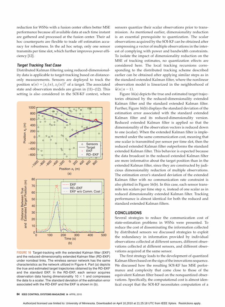
84 IEEE CONTROL SYSTEMS MAGAZINE » APRIL 2010
reduction for WSNs with a fusion center offers better MSE
performance because all available data at each time instant
are gathered and processed at the fusion center. Their ad
hoc counterparts are flexible to trade off estimation accu-
racy for robustness. In the ad hoc setup, only one sensor
transmits per time slot, which further improves power effi-
ciency [12].
Target Tracking Test Case
Distributed Kalman filtering using reduced-dimensional-
ity data is applicable to target-tracking based on distance-
only measurements. Sensors are deployed to track the
position x (n) 5 3x1 (n) , x2 (n)4T of a target. The associated
state and observation models are given in (11)–(12). This
setting is also considered in the SOI-KF context, where
sensors quantize their scalar observations prior to trans-
mission. As mentioned earlier, dimensionality reduction
is an essential prerequisite to quantization. The scalar
observations acquired by the SOI-KF can be obtained after
compressing a vector of multiple observations in the inter-
est of complying with power and bandwidth constraints.
To isolate the impact of dimensionality reduction on the
MSE of tracking estimates, no quantization effects are
considered here. The local tracking recursions corre-
sponding to the distributed tracking scheme described
earlier can be obtained after applying similar steps as in
the standard extended Kalman filter, where the nonlinear
observation model is linearized in the neighborhood of
x (n|n 2 1) .
Figure 16(a) depicts the true and estimated target trajec-
tories obtained by the reduced-dimensionality extended
Kalman filter and the standard extended Kalman filter.
Further, Figure 16(b) displays the standard deviation of the
estimation error associated with the standard extended
Kalman filter and its reduced-dimensionality version.
Reduced extended Kalman filter is applied so that the
dimensionality of the observation vectors is reduced down
to one (scalar). When the extended Kalman filter is imple-
mented under the same communication cost, meaning that
one scalar is transmitted per sensor per time slot, then the
reduced extended Kalman filter outperforms the standard
extended Kalman filter. This behavior is expected because
the data broadcast in the reduced extended Kalman filter
are more informative about the target position than in the
extended Kalman filter, since they are constructed by judi-
cious dimensionality reduction of multiple observations.
The estimation error’s standard deviation of the extended
Kalman filter with no communication rate constraint is
also plotted in Figure 16(b). In this case, each sensor trans-
mits ten scalars per time step n, instead of one scalar as in
reduced dimensionality extended Kalman filter. Tracking
performance is almost identical for both the reduced and
standard extended Kalman filters.
CONCLUSIONSSeveral strategies to reduce the communication cost of
state-estimation problems in WSNs were presented. To
reduce the cost of disseminating the information collected
by distributed sensors we discussed strategies to exploit
the redundancy in information provided by individual
observations collected at different sensors, different obser-
vations collected at different sensors, and different obser-
vations acquired at the same sensor.
The first strategy leads to the development of quantized
Kalman filters based on the sign of the innovations sequence.
We discussed how the resulting SOI-KF has MSE perfor-
mance and complexity that come close to those of the
equivalent Kalman filter based on the nonquantized obser-
vations. Specifically, the computational cost is almost iden-
tical except that the SOI-KF necessitates computation of a
−100
0
−800
−600
−400
−200 0
200
400
600
800
−600
−400
−200
0
200
400
600
800
1000
Po
sitio
n x
2 (
m)
Position x1 (m)
(a)
SensorsTargetEKFRD−EKF
0 100 200 300 400 5000
10
20
30
40
50
60
70
80
Time (s)
(b)
Dis
tance B
etw
een T
rue
and E
stim
ate
d T
arg
et P
ositio
n (
m)
EKFRD−EKFEKF w/o Comm. Cost
FIGURE 16 Target-tracking with the extended Kalman filter (EKF)
and the reduced-dimensionality extended Kalman filter (RD-EKF)
under nonideal links. The wireless sensor network has the same
characteristics as the network utilized in Figure 4. Part (a) depicts
the true and estimated target trajectories obtained by the RD-EKF
and the standard EKF. In the RD-EKF, each sensor acquires
observation data having dimensionality 10 3 1 and compresses
the data to a scalar. The standard deviation of the estimation error
associated with the RD-EKF and the EKF is shown in (b).
Authorized licensed use limited to: University of Minnesota. Downloaded on April 10,2010 at 21:25:18 UTC from IEEE Xplore. Restrictions apply.
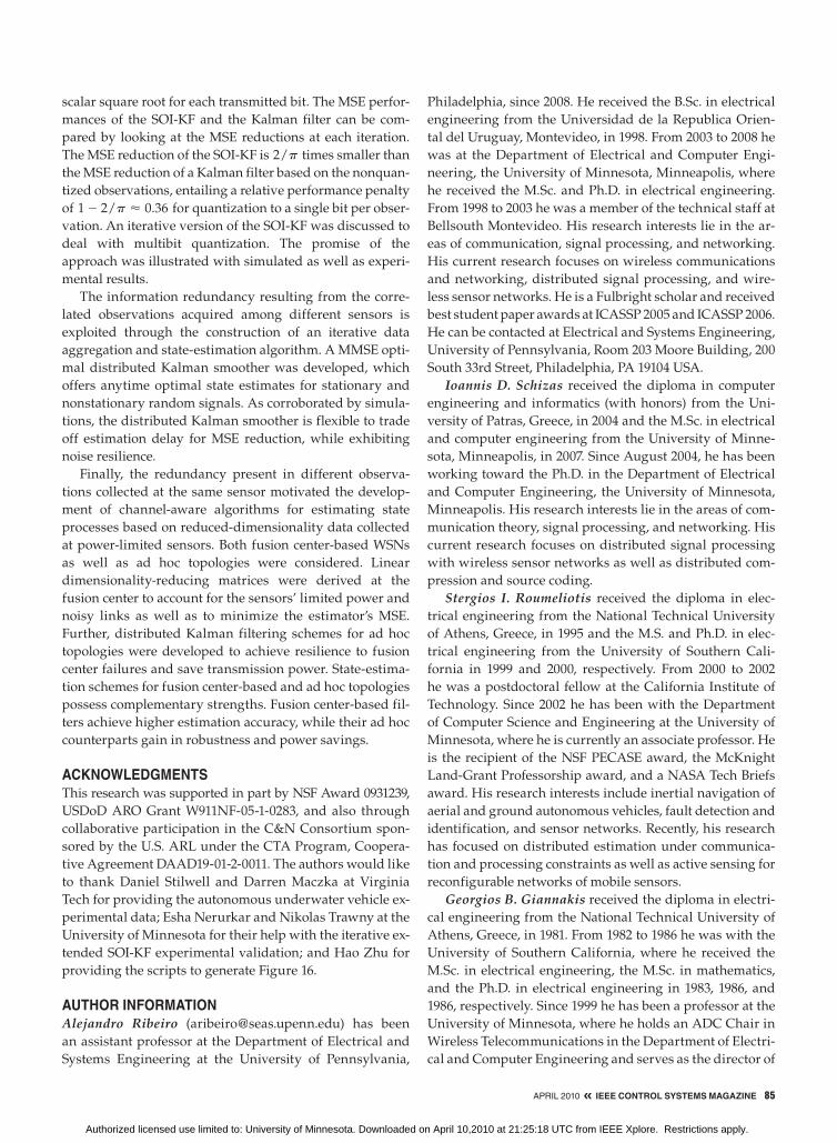
APRIL 2010 « IEEE CONTROL SYSTEMS MAGAZINE 85
scalar square root for each transmitted bit. The MSE perfor-
mances of the SOI-KF and the Kalman filter can be com-
pared by looking at the MSE reductions at each iteration.
The MSE reduction of the SOI-KF is 2/p times smaller than
the MSE reduction of a Kalman filter based on the nonquan-
tized observations, entailing a relative performance penalty
of 1 2 2/p < 0.36 for quantization to a single bit per obser-
vation. An iterative version of the SOI-KF was discussed to
deal with multibit quantization. The promise of the
approach was illustrated with simulated as well as experi-
mental results.
The information redundancy resulting from the corre-
lated observations acquired among different sensors is
exploited through the construction of an iterative data
aggregation and state-estimation algorithm. A MMSE opti-
mal distributed Kalman smoother was developed, which
offers anytime optimal state estimates for stationary and
nonstationary random signals. As corroborated by simula-
tions, the distributed Kalman smoother is flexible to trade
off estimation delay for MSE reduction, while exhibiting
noise resilience.
Finally, the redundancy present in different observa-
tions collected at the same sensor motivated the develop-
ment of channel-aware algorithms for estimating state
processes based on reduced-dimensionality data collected
at power-limited sensors. Both fusion center-based WSNs
as well as ad hoc topologies were considered. Linear
dimensionality-reducing matrices were derived at the
fusion center to account for the sensors’ limited power and
noisy links as well as to minimize the estimator’s MSE.
Further, distributed Kalman filtering schemes for ad hoc
topologies were developed to achieve resilience to fusion
center failures and save transmission power. State-estima-
tion schemes for fusion center-based and ad hoc topologies
possess complementary strengths. Fusion center-based fil-
ters achieve higher estimation accuracy, while their ad hoc
counterparts gain in robustness and power savings.
ACKNOWLEDGMENTSThis research was supported in part by NSF Award 0931239,
USDoD ARO Grant W911NF-05-1-0283, and also through
collaborative participation in the C&N Consortium spon-
sored by the U.S. ARL under the CTA Program, Coopera-
tive Agreement DAAD19-01-2-0011. The authors would like
to thank Daniel Stilwell and Darren Maczka at Virginia
Tech for providing the autonomous underwater vehicle ex-
perimental data; Esha Nerurkar and Nikolas Trawny at the
University of Minnesota for their help with the iterative ex-
tended SOI-KF experimental validation; and Hao Zhu for
providing the scripts to generate Figure 16.
AUTHOR INFORMATIONAlejandro Ribeiro ([email protected]) has been
an assistant professor at the Department of Electrical and
Systems Engineering at the University of Pennsylvania,
Philadelphia, since 2008. He received the B.Sc. in electrical
engineering from the Universidad de la Republica Orien-
tal del Uruguay, Montevideo, in 1998. From 2003 to 2008 he
was at the Department of Electrical and Computer Engi-
neering, the University of Minnesota, Minneapolis, where
he received the M.Sc. and Ph.D. in electrical engineering.
From 1998 to 2003 he was a member of the technical staff at
Bellsouth Montevideo. His research interests lie in the ar-
eas of communication, signal processing, and networking.
His current research focuses on wireless communications
and networking, distributed signal processing, and wire-
less sensor networks. He is a Fulbright scholar and received
best student paper awards at ICASSP 2005 and ICASSP 2006.
He can be contacted at Electrical and Systems Engineering,
University of Pennsylvania, Room 203 Moore Building, 200
South 33rd Street, Philadelphia, PA 19104 USA.
Ioannis D. Schizas received the diploma in computer
engineering and informatics (with honors) from the Uni-
versity of Patras, Greece, in 2004 and the M.Sc. in electrical
and computer engineering from the University of Minne-
sota, Minneapolis, in 2007. Since August 2004, he has been
working toward the Ph.D. in the Department of Electrical
and Computer Engineering, the University of Minnesota,
Minneapolis. His research interests lie in the areas of com-
munication theory, signal processing, and networking. His
current research focuses on distributed signal processing
with wireless sensor networks as well as distributed com-
pression and source coding.
Stergios I. Roumeliotis received the diploma in elec-
trical engineering from the National Technical University
of Athens, Greece, in 1995 and the M.S. and Ph.D. in elec-
trical engineering from the University of Southern Cali-
fornia in 1999 and 2000, respectively. From 2000 to 2002
he was a postdoctoral fellow at the California Institute of
Technology. Since 2002 he has been with the Department
of Computer Science and Engineering at the University of
Minnesota, where he is currently an associate professor. He
is the recipient of the NSF PECASE award, the McKnight
Land-Grant Professorship award, and a NASA Tech Briefs
award. His research interests include inertial navigation of
aerial and ground autonomous vehicles, fault detection and
identification, and sensor networks. Recently, his research
has focused on distributed estimation under communica-
tion and processing constraints as well as active sensing for
reconfigurable networks of mobile sensors.
Georgios B. Giannakis received the diploma in electri-
cal engineering from the National Technical University of
Athens, Greece, in 1981. From 1982 to 1986 he was with the
University of Southern California, where he received the
M.Sc. in electrical engineering, the M.Sc. in mathematics,
and the Ph.D. in electrical engineering in 1983, 1986, and
1986, respectively. Since 1999 he has been a professor at the
University of Minnesota, where he holds an ADC Chair in
Wireless Telecommunications in the Department of Electri-
cal and Computer Engineering and serves as the director of
Authorized licensed use limited to: University of Minnesota. Downloaded on April 10,2010 at 21:25:18 UTC from IEEE Xplore. Restrictions apply.
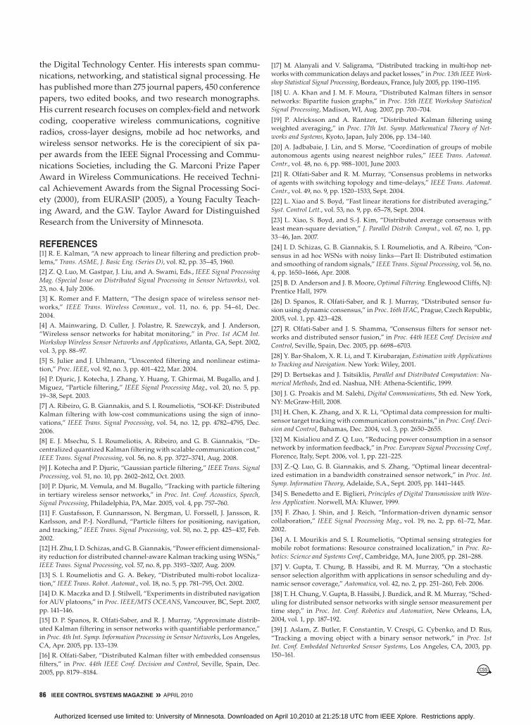
86 IEEE CONTROL SYSTEMS MAGAZINE » APRIL 2010
the Digital Technology Center. His interests span commu-
nications, networking, and statistical signal processing. He
has published more than 275 journal papers, 450 conference
papers, two edited books, and two research monographs.
His current research focuses on complex-field and network
coding, cooperative wireless communications, cognitive
radios, cross-layer designs, mobile ad hoc networks, and
wireless sensor networks. He is the corecipient of six pa-
per awards from the IEEE Signal Processing and Commu-
nications Societies, including the G. Marconi Prize Paper
Award in Wireless Communications. He received Techni-
cal Achievement Awards from the Signal Processing Soci-
ety (2000), from EURASIP (2005), a Young Faculty Teach-
ing Award, and the G.W. Taylor Award for Distinguished
Research from the University of Minnesota.
REFERENCES[1] R. E. Kalman, “A new approach to linear filtering and prediction prob-
lems,” Trans. ASME, J. Basic Eng. (Series D), vol. 82, pp. 35–45, 1960.
[2] Z. Q. Luo, M. Gastpar, J. Liu, and A. Swami, Eds., IEEE Signal Processing Mag. (Special Issue on Distributed Signal Processing in Sensor Networks), vol.
23, no. 4, July 2006.
[3] K. Romer and F. Mattern, “The design space of wireless sensor net-
works,” IEEE Trans. Wireless Commun., vol. 11, no. 6, pp. 54–61, Dec.
2004.
[4] A. Mainwaring, D. Culler, J. Polastre, R. Szewczyk, and J. Anderson,
“Wireless sensor networks for habitat monitoring,” in Proc. 1st ACM Int. Workshop Wireless Sensor Networks and Applications, Atlanta, GA, Sept. 2002,
vol. 3, pp. 88–97.
[5] S. Julier and J. Uhlmann, “Unscented filtering and nonlinear estima-
tion,” Proc. IEEE, vol. 92, no. 3, pp. 401–422, Mar. 2004.
[6] P. Djuric, J. Kotecha, J. Zhang, Y. Huang, T. Ghirmai, M. Bugallo, and J.
Miguez, “Particle filtering,” IEEE Signal Processing Mag., vol. 20, no. 5, pp.
19–38, Sept. 2003.
[7] A. Ribeiro, G. B. Giannakis, and S. I. Roumeliotis, “SOI-KF: Distributed
Kalman filtering with low-cost communications using the sign of inno-
vations,” IEEE Trans. Signal Processing, vol. 54, no. 12, pp. 4782–4795, Dec.
2006.
[8] E. J. Msechu, S. I. Roumeliotis, A. Ribeiro, and G. B. Giannakis, “De-
centralized quantized Kalman filtering with scalable communication cost,”
IEEE Trans. Signal Processing, vol. 56, no. 8, pp. 3727–3741, Aug. 2008.
[9] J. Kotecha and P. Djuric, “Gaussian particle filtering,” IEEE Trans. Signal Processing, vol. 51, no. 10, pp. 2602–2612, Oct. 2003.
[10] P. Djuric, M. Vemula, and M. Bugallo, “Tracking with particle filtering
in tertiary wireless sensor networks,” in Proc. Int. Conf. Acoustics, Speech, Signal Processing, Philadelphia, PA, Mar. 2005, vol. 4, pp. 757–760.
[11] F. Gustafsson, F. Gunnarsson, N. Bergman, U. Forssell, J. Jansson, R.
Karlsson, and P.-J. Nordlund, “Particle filters for positioning, navigation,
and tracking,” IEEE Trans. Signal Processing, vol. 50, no. 2, pp. 425–437, Feb.
2002.
[12] H. Zhu, I. D. Schizas, and G. B. Giannakis, “Power efficient dimensional-
ity reduction for distributed channel-aware Kalman tracking using WSNs,”
IEEE Trans. Signal Processing, vol. 57, no. 8, pp. 3193–3207, Aug. 2009.
[13] S. I. Roumeliotis and G. A. Bekey, “Distributed multi-robot localiza-
tion,” IEEE Trans. Robot. Automat., vol. 18, no. 5, pp. 781–795, Oct. 2002.
[14] D. K. Maczka and D. J. Stilwell, “Experiments in distributed navigation
for AUV platoons,” in Proc. IEEE/MTS OCEANS, Vancouver, BC, Sept. 2007,
pp. 141–146.
[15] D. P. Spanos, R. Olfati-Saber, and R. J. Murray, “Approximate distrib-
uted Kalman filtering in sensor networks with quantifiable performance,”
in Proc. 4th Int. Symp. Information Processing in Sensor Networks, Los Angeles,
CA, Apr. 2005, pp. 133–139.
[16] R. Olfati-Saber, “Distributed Kalman filter with embedded consensus
filters,” in Proc. 44th IEEE Conf. Decision and Control, Seville, Spain, Dec.
2005, pp. 8179–8184.
[17] M. Alanyali and V. Saligrama, “Distributed tracking in multi-hop net-
works with communication delays and packet losses,” in Proc. 13th IEEE Work-shop Statistical Signal Processing, Bordeaux, France, July 2005, pp. 1190–1195.
[18] U. A. Khan and J. M. F. Moura, “Distributed Kalman filters in sensor
networks: Bipartite fusion graphs,” in Proc. 15th IEEE Workshop Statistical Signal Processing, Madison, WI, Aug. 2007, pp. 700–704.
[19] P. Alricksson and A. Rantzer, “Distributed Kalman filtering using
weighted averaging,” in Proc. 17th Int. Symp. Mathematical Theory of Net-works and Systems, Kyoto, Japan, July 2006, pp. 134–140.
[20] A. Jadbabaie, J. Lin, and S. Morse, “Coordination of groups of mobile
autonomous agents using nearest neighbor rules,” IEEE Trans. Automat. Contr., vol. 48, no. 6, pp. 988–1001, June 2003.
[21] R. Olfati-Saber and R. M. Murray, “Consensus problems in networks
of agents with switching topology and time-delays,” IEEE Trans. Automat. Contr., vol. 49, no. 9, pp. 1520–1533, Sept. 2004.
[22] L. Xiao and S. Boyd, “Fast linear iterations for distributed averaging,”
Syst. Control Lett., vol. 53, no. 9, pp. 65–78, Sept. 2004.
[23] L. Xiao, S. Boyd, and S.-J. Kim, “Distributed average consensus with
least mean-square deviation,” J. Parallel Distrib. Comput., vol. 67, no. 1, pp.
33–46, Jan. 2007.
[24] I. D. Schizas, G. B. Giannakis, S. I. Roumeliotis, and A. Ribeiro, “Con-
sensus in ad hoc WSNs with noisy links—Part II: Distributed estimation
and smoothing of random signals,” IEEE Trans. Signal Processing, vol. 56, no.
4, pp. 1650–1666, Apr. 2008.
[25] B. D. Anderson and J. B. Moore, Optimal Filtering. Englewood Cliffs, NJ:
Prentice Hall, 1979.
[26] D. Spanos, R. Olfati-Saber, and R. J. Murray, “Distributed sensor fu-
sion using dynamic consensus,” in Proc. 16th IFAC, Prague, Czech Republic,
2005, vol. 1, pp. 423–428.
[27] R. Olfati-Saber and J. S. Shamma, “Consensus filters for sensor net-
works and distributed sensor fusion,” in Proc. 44th IEEE Conf. Decision and Control, Seville, Spain, Dec. 2005, pp. 6698–6703.
[28] Y. Bar-Shalom, X. R. Li, and T. Kirubarajan, Estimation with Applications to Tracking and Navigation. New York: Wiley, 2001.
[29] D. Bertsekas and J. Tsitsiklis, Parallel and Distributed Computation: Nu-merical Methods, 2nd ed. Nashua, NH: Athena-Scientific, 1999.
[30] J. G. Proakis and M. Salehi, Digital Communications, 5th ed. New York,
NY: McGraw-Hill, 2008.
[31] H. Chen, K. Zhang, and X. R. Li, “Optimal data compression for multi-
sensor target tracking with communication constraints,” in Proc. Conf. Deci-sion and Control, Bahamas, Dec. 2004, vol. 3, pp. 2650–2655.
[32] M. Kisialiou and Z. Q. Luo, “Reducing power consumption in a sensor
network by information feedback,” in Proc. European Signal Processing Conf., Florence, Italy, Sept. 2006, vol. 1, pp. 221–225.
[33] Z.-Q. Luo, G. B. Giannakis, and S. Zhang, “Optimal linear decentral-
ized estimation in a bandwidth constrained sensor network,” in Proc. Int. Symp. Information Theory, Adelaide, S.A., Sept. 2005, pp. 1441–1445.
[34] S. Benedetto and E. Biglieri, Principles of Digital Transmission with Wire-less Application. Norwell, MA: Kluwer, 1999.
[35] F. Zhao, J. Shin, and J. Reich, “Information-driven dynamic sensor
collaboration,” IEEE Signal Processing Mag., vol. 19, no. 2, pp. 61–72, Mar.
2002.
[36] A. I. Mourikis and S. I. Roumeliotis, “Optimal sensing strategies for
mobile robot formations: Resource constrained localization,” in Proc. Ro-botics: Science and Systems Conf., Cambridge, MA, June 2005, pp. 281–288.
[37] V. Gupta, T. Chung, B. Hassibi, and R. M. Murray, “On a stochastic
sensor selection algorithm with applications in sensor scheduling and dy-
namic sensor coverage,” Automatica, vol. 42, no. 2, pp. 251–260, Feb. 2006.
[38] T. H. Chung, V. Gupta, B. Hassibi, J. Burdick, and R. M. Murray, “Sched-
uling for distributed sensor networks with single sensor measurement per
time step,” in Proc. Int. Conf. Robotics and Automation, New Orleans, LA,
2004, vol. 1, pp. 187–192.
[39] J. Aslam, Z. Butler, F. Constantin, V. Crespi, G. Cybenko, and D. Rus,
“Tracking a moving object with a binary sensor network,” in Proc. 1st Int. Conf. Embedded Networked Sensor Systems, Los Angeles, CA, 2003, pp.
150–161.
Authorized licensed use limited to: University of Minnesota. Downloaded on April 10,2010 at 21:25:18 UTC from IEEE Xplore. Restrictions apply.