Embed Size (px)
Citation preview

A&A 609, A113 (2018)DOI: 10.1051/0004-6361/201730386c© ESO 2018
Astronomy&Astrophysics
Solar system science with ESA EuclidB. Carry1, 2
1 Université Côte d’Azur, Observatoire de la Côte d’Azur, CNRS, Lagrange, 06304 Nice, France2 IMCCE, Observatoire de Paris, PSL Research University, CNRS, Sorbonne Universités, UPMC Univ. Paris 06, Univ. Lille, France
e-mail: [email protected]
Received 2 January 2017 / Accepted 3 November 2017
ABSTRACT
Context. The ESA Euclid mission has been designed to map the geometry of the dark Universe. Scheduled for launch in 2020, it willconduct a six-year visible and near-infrared imaging and spectroscopic survey over 15 000 deg2 down to VAB ∼ 24.5. Although thesurvey will avoid ecliptic latitudes below 15◦, the survey pattern in repeated sequences of four broadband filters seems well-adaptedto detect and characterize solar system objects (SSOs).Aims. We aim at evaluating the capability of Euclid of discovering SSOs and of measuring their position, apparent magnitude, andspectral energy distribution. We also investigate how the SSO orbits, morphology (activity and multiplicity), physical properties(rotation period, spin orientation, and 3D shape), and surface composition can be determined based on these measurements.Methods. We used the current census of SSOs to extrapolate the total amount of SSOs that will be detectable by Euclid, that is, objectswithin the survey area and brighter than the limiting magnitude. For each different population of SSO, from neighboring near-Earthasteroids to distant Kuiper-belt objects (KBOs) and including comets, we compared the expected Euclid astrometry, photometry,and spectroscopy with the SSO properties to estimate how Euclid will constrain the SSOs dynamical, physical, and compositionalproperties.Results. With the current survey design, about 150 000 SSOs, mainly from the asteroid main-belt, should be observable by Euclid.These objects will all have high inclination, which is a difference to many SSO surveys that focus on the ecliptic plane. Euclid may beable to discover several 104 SSOs, in particular, distant KBOs at high declination. The Euclid observations will consist of a suite offour sequences of four measurements and will refine the spectral classification of SSOs by extending the spectral coverage providedby Gaia and the LSST, for instance, to 2 microns. Combined with sparse photometry such as measured by Gaia and the LSST, thetime-resolved photometry will contribute to determining the SSO rotation period, spin orientation, and 3D shape model. The sharpand stable point-spread function of Euclid will also allow us to resolve binary systems in the Kuiper belt and detect activity aroundCentaurs.Conclusions. The depth of the Euclid survey (VAB ∼ 24.5), its spectral coverage (0.5 to 2.0 µm), and its observation cadence hasgreat potential for solar system research. A dedicated processing for SSOs is being set up within the Euclid consortium to produceastrometry catalogs, multicolor and time-resolved photometry, and spectral classification of some 105 SSOs, which will be deliveredas Legacy Science.
Key words. methods: statistical – minor planets, asteroids: general – Kuiper belt: general – comets: general
1. Introduction
The second mission in ESA’s Cosmic Vision program, Euclid isa wide-field space mission dedicated to the study of dark energyand dark matter through mapping weak gravitational lensing(Laureijs et al. 2011). It is equipped with a silicon-carbide 1.2 maperture Korsch telescope and two instruments: a VISible imag-ing camera, and a Near Infrared Spectrometer and Photometer(VIS and NISP; see Cropper et al. 2014; Maciaszek et al. 2014).The mission design combines a large field of view (FoV, 0.57deg2) with high angular resolution (pixel scales of 0.1′′ and0.3′′ for VIS and NISP, corresponding to the diffraction limitat 0.6 and 1.7 µm).
Scheduled for a launch in 2020 and operating during sixyears from the Sun-Earth Lagrange L2 point, Euclid will carryout an imaging and spectroscopic survey of the extragalactic skyof 15 000 deg2 (the Wide Survey), avoiding galactic latitudeslower than 30◦ and ecliptic latitudes below 15◦ (Fig. 1), total-ing 35 000 pointings. A second survey, two magnitudes deeperand located at very high ecliptic latitudes, will cover 40 deg2
spread across three areas (the Deep Survey). Additionally,7000 observations of 1200 calibration fields, mainly located
at −10◦ and +10◦ galactic latitude, will be acquired duringthe course of the mission to monitor the stability of the tele-scope point-spread function (PSF), and assess the photometricand spectroscopic accuracy of the mission.
Euclid imaging detection limits are required at mAB = 24.5(10σ on a 1′′ extended source) with VIS, and mAB = 24 (5σpoint source) in the Y , J, and H filters with NISP. Spectro-scopic requirements are to cover the same near-infrared wave-length range at a resolving power of 380 and to detect at 3.5σan emission line at 3 × 10⁻¹⁶ erg cm−1 s−1 (on a 1′′ extendedsource). The NISP implementation consists of two grisms, red(1.25 to 1.85 µm) and blue (0.92 to 1.25 µm, usage of which willbe limited to the Deep Survey), providing a continuum sensitiv-ity to mAB ≈ 21. To achieve these goals, the following surveyoperations were designed:
1. The observations will consist of a step-and-stare tiling mode,in which both instruments target the common 0.57 deg2 FOVbefore the telescope slews to other coordinates.
2. Each tile will be visited only once, with the exception of theDeep Survey, in which each tile will be pointed at 40 times,
Article published by EDP Sciences A113, page 1 of 15

A&A 609, A113 (2018)
0h
00
6h
00
12
h0
012
h0
0
18
h0
0
-90
-60 -60
-30 -30
0 0
3 0 3 0
6 0 6 0
9 0
Wide Survey
Calibration
Ecliptic plane
Galactic plane
7600
7800
8000
8200
8400
8600
8800
9000
9200
9400
9600
MJD
20
00
.0
Fig. 1. Expected coverage of the Euclid Wide Survey (called the reference survey), color-coded by observing epoch, in an Aitoff projection ofecliptic coordinates. The horizontal gap corresponds to low ecliptic latitudes (the cyan line represents the ecliptic plane), and the circular gap tolow galactic latitudes (the deep blue line stands for the galactic plane). The black squares filled with yellow are the calibration fields, which are tobe repeatedly observed during the six years of the mission, to assess the stability and accuracy of the Euclid PSF, photometry, and spectroscopy.
Fig. 2. Observation sequence for each pointing. The observing block,composed of a simultaneous VIS and NISP/spectroscopy exposure andthree NISP/imaging exposures (Y , J, H), is repeated four times, withsmall jitters (100′′ × 50′′). The blue boxes F and S stand for over-heads that are due to the rotation of the filter wheel and shutter open-ing/closure. Figure adapted from Laureijs et al. (2011).
and the calibration fields, which will be observed 5 timeseach on average.
3. The filling pattern of the survey will follow the lines of eclip-tic longitude at quadrature. Current survey planning fore-sees a narrow distribution of the solar elongation of Ψ =91.0 ± 1.5◦ only; the range of solar elongation available tothe telescope is limited to 87◦–110◦.
4. The observation of each tile will be subdivided into four ob-serving blocks that differ by only small jitters (100′′ × 50′′).These small pointing offsets will allow to fill the gaps be-tween the detectors that make up the focal plane of each in-strument. In this way, 95% of the sky will be covered by threeblocks, and 50% by four blocks.
5. In each block, near-infrared slitless spectra will be obtainedwith NISP simultaneously with a visible image with VIS,with an integration time of 565 s. This integration time im-plies a saturation limit of VAB ≈ 17 for a point-like source.Then, three NISP images will be taken with the Y , J, andH near-infrared filters, with integration times of 121, 116,and 81 s, respectively (Fig. 2).
All these characteristics make the Euclid survey a potentialprime data set for legacy science. In particular, the access to
the near-infrared sky, about seven magnitudes fainter than theDENIS and 2MASS (Epchtein et al. 1994; Skrutskie et al. 2006)surveys, and two to three magnitudes fainter than the cur-rent ESO VISTA Hemispherical Survey (VHS; McMahon et al.2013), makes Euclid suitable for a surface characterizationof solar system objects (SSOs), especially in an era richin surveys that only operate in visible wavelengths, suchas the Sloan Digital Sky Survey (SDSS), Pan-STARRS,ESA Gaia, and the Large Synoptic Sky Survey (LSST)(Abazajian et al. 2003; Jewitt 2003; Gaia Collaboration 2016;LSST Science Collaboration et al. 2009).
We discuss here the potential of the Euclid mission forsolar system science. In the following, we consider the fol-lowing populations of SSOs, defined by their orbital elements(Appendix A):
– near-Earth asteroids (NEAs), including the Aten, Apollo,and Amor classes, whose orbits cross the orbits of terrestrialplanets;
– Mars-crossers (MCs), a transitory population between the as-teroid main belt and near-Earth space;
– main-belt asteroids (MBA) in the principal reservoir of as-teroids in the solar system, between Mars and Jupiter, splitinto Hungarian, inner main-belt (IMB), middle main-belt(MMB), outer main-belt (OMB), Cybele, and Hilda;
– Jupiter trojans (Trojans), orbiting the Sun at the Lagrange L4and L5 points of the Sun-Jupiter system;
– Centaurs whose orbits cross the orbits of giant planets;– Kuiper-belt objects (KBOs) farther away than Neptune, di-
vided into detached, resonant, and scattered-disk objects(SDO), and inner, main, and outer classical belt (ICB, MCB,and OCB); and
– comets from the outskirts of the solar system on highly ec-centric orbits that are characterized by activity (coma) atshort heliocentric distances.
The discussion is organized as follows: the expected numberof SSO observations is presented in Sect. 2, and the difficul-ties we expect for these observations are described in Sect. 3.The problems of source identification and the contribution toastrometry and orbit determination are discussed in Sect. 4.Then the potential for spectral characterization from VIS andNISP photometry is detailed in Sect. 5, and the same is done for
A113, page 2 of 15

B. Carry: Solar system science with ESA Euclid
173.2 173.4 173.6
16.4
16.6
16.8
17.0
173.2 173.4 173.6Ecliptic longitude (o)
16.4
16.6
16.8
17.0
Eclip
tic latitu
de (
o)
VIS
Y
J
H
Filters
t0 = 2022−06−16T20:26:05 Survey field 15117
2014 WQ501
t0+10s
t0+1058s
t0+2106s
t0+3154s
6"
Magnified view
77.6 77.8 78.0 78.2
0.8
1.0
1.2
1.4
77.6 77.8 78.0 78.2Ecliptic longitude (o)
0.8
1.0
1.2
1.4
Eclip
tic latitu
de (
o)
VIS
Y
J
H
Filters
t0 = 2022−03−09T20:37:37 Calibration field 13165
Fig. 3. Examples of the contamination of Euclid FOV by SSOs. Left: survey field 15117 centered on (RA, Dec) = (167.218◦, +12.740◦) andstarting on 2022 June 16 at 20:26:05 UTC. The successive trails impressed by the 6 known SSOs during the Euclid hour-long sequence ofVIS-NISP imaging observations are drawn in different colors, one for each filter (VIS, Y , J, and H). We can expect about a hundred times moreSSOs at the limiting magnitude of Euclid (e.g., Fig. 4). The inset is a magnified view of 2014 WQ501, a main-belt asteroid, illustrating the highlyelongated shape of an SSO in Euclid frames. The scale bar of 6′′ corresponds to 60 pixels in VIS frames and 20 pixels in NISP. The timingsreported are the starting time of the VIS exposures. The slitless spectra will be acquired by NISP simultaneously with the VIS images. Right:calibration field 13 165 centered on (RA, Dec) = (76.785◦, +23.988◦) and starting on 2022 March 9 at 20:37:37 UTC. There are 117 known SSOsin the field, and here also, a hundred times more SSOs will be detected at the limiting magnitude of Euclid.
NISP spectroscopy in Sect. 6. The Euclid capabilities for directlyimaging satellites and SSO activity are presented in Sect. 7, andthe contribution of Euclid to the 3D shape and binarity modelingfrom light curves is described in Sect. 8.
2. Expected number of SSO observations
Although the Euclid Wide survey will avoid the ecliptic plane(Fig. 1), its observing sequence is by chance well adapted todetect moving objects. As described above, each FoV will beimaged 16 times in one hour in four repeated blocks. Given thepixel scale of the VIS and NISP cameras of 0.1′′ and 0.3′′, anySSO with an apparent motion higher than ≈0.2′′/h should there-fore be detected by its trailed appearance and/or motion acrossthe different frames (Fig. 3).
To estimate the number of SSOs that might be detected byEuclid, we first built the cumulative size distribution (CSD)of each population. We used the absolute magnitude H as aproxy for the diameter D. The relation between these two isD(km) = 1329p−1/2
V 10−0.2H (e.g., Bowell et al. 1989), where pVis the surface albedo in V, which quantifies its capability of re-flecting light. Minor planets, especially asteroids, tend to be verydark, and their albedo is generally very low, from a few percentsto ≈30% (see, e.g., Mainzer et al. 2011).
We retrieved the absolute magnitude from the astorbdatabase (Bowell et al. 1993), with the exception of comets,which are not listed in astorb, and for which we used the com-piled data by Snodgrass et al. (2011). The challenge was thento extrapolate the observed distributions (shown as solid linesin Fig. 4) to smaller sizes. Most are close to power-law distribu-tions (Dohnanyi 1969) in the form dN/dH ∝ 10γH , with different
slopes γ. We model each population below and represent themwith dashed lines in Fig. 4:
– NEAs: we used the synthetic population by Granvik et al.(2016), which is very similar to the population used byHarris & D’Abramo (2015). However, we took a conserva-tive approach and increased the uncertainty of the model toencompass both estimates.
– MCs: no dedicated study of the CSD of MCs is available.We therefore took the NEA model above, scaled by a factorof three, to match the currently known MC population. Theupper estimate was taken as a power-law fit to the currentpopulation with γ = 0.41, and the lower estimate is that ofthe scaled NEA model by Granvik et al. (2016), reduced bya factor of two.
– MBAs: we used the knee distribution by Gladman et al.(2009), in which large objects (H ∈ [11, 15]) follow a steepslope (γ ∼ 0.5), while smaller asteroids follow a shallowerslope of γ = 0.30 ± 0.02 in the range H ∈ [15, 18], af-ter which no constraint is available. This model is scaled to25 954 asteroids at H = 15. These authors found the CSD tobe very smooth in this absolute magnitude range compared toearlier works (Jedicke & Metcalfe 1998; Ivezic et al. 2001;Wiegert et al. 2007). We modified their model only slightlyby changing the slope at H = 15.25 instead of H = 15: theshallower slope does no longer fit the observed data belowH = 15.25. The observing strategy by Gladman et al. (2009)was indeed aimed at constraining the faint end of the CSD,and the constraints on large bodies was weak (only a smallsky area had been targeted).
– Trojans: we used the model of Jewitt et al. (2000), withγ = 0.4 ± 0.06. More recently, Grav et al. (2011) found
A113, page 3 of 15
A&A 609, A113 (2018)
2 4 6 8 10 12 14 16 18 20 22 24
100
101
102
103
104
105
106
107
108
2 4 6 8 10 12 14 16 18 20 22 24Absolute magnitude (H)
100
101
102
103
104
105
106
107
108
Cum
ula
tive n
um
ber
N(<
H)
Comet
KBO
Centaur
MB
Outer Solar System
Margin for
discovery
2 4 6 8 10 12 14 16 18 20 22 24
100
101
102
103
104
105
106
107
108
Cum
ula
tive n
um
ber
N(<
H)
Trojan
MB
MC
NEA
Inner Solar System
100 10 1 0.1 kmDiameter
PopulationsKnownSyntheticby Euclid
DetectionsPhoton−limitedSaturated
Margin for
discovery
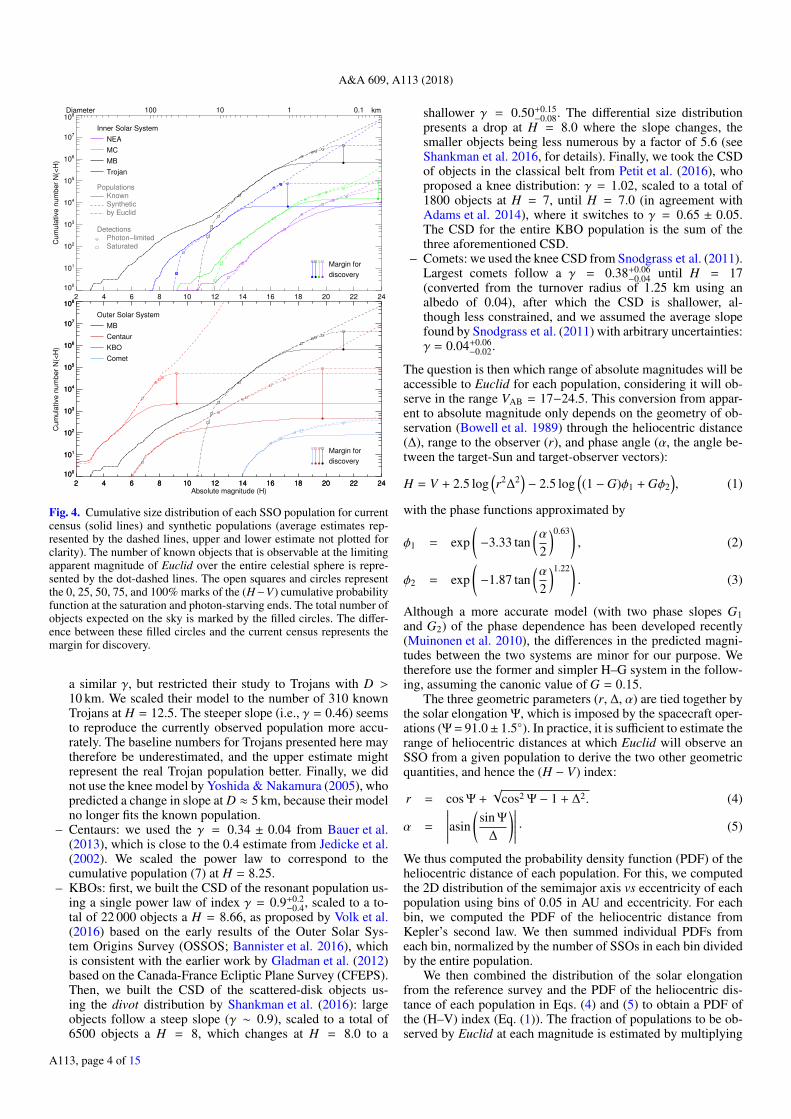
Fig. 4. Cumulative size distribution of each SSO population for currentcensus (solid lines) and synthetic populations (average estimates rep-resented by the dashed lines, upper and lower estimate not plotted forclarity). The number of known objects that is observable at the limitingapparent magnitude of Euclid over the entire celestial sphere is repre-sented by the dot-dashed lines. The open squares and circles representthe 0, 25, 50, 75, and 100% marks of the (H−V) cumulative probabilityfunction at the saturation and photon-starving ends. The total number ofobjects expected on the sky is marked by the filled circles. The differ-ence between these filled circles and the current census represents themargin for discovery.
a similar γ, but restricted their study to Trojans with D >10 km. We scaled their model to the number of 310 knownTrojans at H = 12.5. The steeper slope (i.e., γ = 0.46) seemsto reproduce the currently observed population more accu-rately. The baseline numbers for Trojans presented here maytherefore be underestimated, and the upper estimate mightrepresent the real Trojan population better. Finally, we didnot use the knee model by Yoshida & Nakamura (2005), whopredicted a change in slope at D ≈ 5 km, because their modelno longer fits the known population.
– Centaurs: we used the γ = 0.34 ± 0.04 from Bauer et al.(2013), which is close to the 0.4 estimate from Jedicke et al.(2002). We scaled the power law to correspond to thecumulative population (7) at H = 8.25.
– KBOs: first, we built the CSD of the resonant population us-ing a single power law of index γ = 0.9+0.2
−0.4, scaled to a to-tal of 22 000 objects a H = 8.66, as proposed by Volk et al.(2016) based on the early results of the Outer Solar Sys-tem Origins Survey (OSSOS; Bannister et al. 2016), whichis consistent with the earlier work by Gladman et al. (2012)based on the Canada-France Ecliptic Plane Survey (CFEPS).Then, we built the CSD of the scattered-disk objects us-ing the divot distribution by Shankman et al. (2016): largeobjects follow a steep slope (γ ∼ 0.9), scaled to a total of6500 objects a H = 8, which changes at H = 8.0 to a
shallower γ = 0.50+0.15−0.08. The differential size distribution
presents a drop at H = 8.0 where the slope changes, thesmaller objects being less numerous by a factor of 5.6 (seeShankman et al. 2016, for details). Finally, we took the CSDof objects in the classical belt from Petit et al. (2016), whoproposed a knee distribution: γ = 1.02, scaled to a total of1800 objects at H = 7, until H = 7.0 (in agreement withAdams et al. 2014), where it switches to γ = 0.65 ± 0.05.The CSD for the entire KBO population is the sum of thethree aforementioned CSD.
– Comets: we used the knee CSD from Snodgrass et al. (2011).Largest comets follow a γ = 0.38+0.06
−0.04 until H = 17(converted from the turnover radius of 1.25 km using analbedo of 0.04), after which the CSD is shallower, al-though less constrained, and we assumed the average slopefound by Snodgrass et al. (2011) with arbitrary uncertainties:γ = 0.04+0.06
−0.02.
The question is then which range of absolute magnitudes will beaccessible to Euclid for each population, considering it will ob-serve in the range VAB = 17−24.5. This conversion from appar-ent to absolute magnitude only depends on the geometry of ob-servation (Bowell et al. 1989) through the heliocentric distance(∆), range to the observer (r), and phase angle (α, the angle be-tween the target-Sun and target-observer vectors):
H = V + 2.5 log(r2∆2
)− 2.5 log
((1 −G)φ1 + Gφ2
), (1)
with the phase functions approximated by
φ1 = exp(−3.33 tan
(α
2
)0.63), (2)
φ2 = exp(−1.87 tan
(α
2
)1.22). (3)
Although a more accurate model (with two phase slopes G1and G2) of the phase dependence has been developed recently(Muinonen et al. 2010), the differences in the predicted magni-tudes between the two systems are minor for our purpose. Wetherefore use the former and simpler H–G system in the follow-ing, assuming the canonic value of G = 0.15.
The three geometric parameters (r, ∆, α) are tied together bythe solar elongation Ψ, which is imposed by the spacecraft oper-ations (Ψ = 91.0± 1.5◦). In practice, it is sufficient to estimate therange of heliocentric distances at which Euclid will observe anSSO from a given population to derive the two other geometricquantities, and hence the (H − V) index:
r = cos Ψ +√
cos2 Ψ − 1 + ∆2. (4)
α =
∣∣∣∣∣∣asin(
sin Ψ
∆
)∣∣∣∣∣∣ · (5)
We thus computed the probability density function (PDF) of theheliocentric distance of each population. For this, we computedthe 2D distribution of the semimajor axis vs eccentricity of eachpopulation using bins of 0.05 in AU and eccentricity. For eachbin, we computed the PDF of the heliocentric distance fromKepler’s second law. We then summed individual PDFs fromeach bin, normalized by the number of SSOs in each bin dividedby the entire population.
We then combined the distribution of the solar elongationfrom the reference survey and the PDF of the heliocentric dis-tance of each population in Eqs. (4) and (5) to obtain a PDF ofthe (H–V) index (Eq. (1)). The fraction of populations to be ob-served by Euclid at each magnitude is estimated by multiplying
A113, page 4 of 15

B. Carry: Solar system science with ESA Euclid
Table 1. Expected number of SSOs observed by Euclid for each population.
Population All-sky fW fC Euclid Absolute magnitude limitsName Nnow NS (%) (%) NE,d NE,o H100 H50 H1
NEA 16062 1.9+1.1−0.6 × 10⁵ 7.2 ± 0.4 0.8 ± 0.1 1.4+1.0
−0.5 × 10⁴ 1.5+1.0−0.6 × 10⁴ 22.75 23.75 26.50
MC 15488 1.2+1.6−0.8 × 10⁵ 9.0 ± 0.6 0.6 ± 0.1 1.0+1.7
−0.8 × 10⁴ 1.2+1.7−0.8 × 10⁴ 21.00 21.25 22.75
MB 674981 4.3+1.0−0.9 × 10⁶ 1.5 ± 0.0 0.7 ± 0.0 8.2+2.5
−2.2 × 10⁴ 9.7+2.5−2.2 × 10⁴ 19.50 20.00 21.25
Trojan 6762 1.3+0.9−0.7 × 10⁵ 5.1 ± 1.5 0.5 ± 0.4 7.1+9.3
−4.9 × 10³ 7.5+9.5−5.0 × 10³ 17.00 17.25 18.25
Centaur 470 1.8+1.4−1.0 × 10⁴ 12.2 ± 0.9 0.6 ± 0.4 2.2+2.1
−1.4 × 10³ 2.2+2.1−1.4 × 10³ 14.75 15.50 18.25
KBO 2331 9.8+2.2−1.9 × 10⁴ 4.9 ± 0.2 0.6 ± 0.1 5.3+1.6
−1.3 × 10³ 5.5+1.6−1.3 × 10³ 8.25 8.75 10.00
Comet 1301 185.2+15.4−13.5×100 19.5 ± 0.5 1.0 ± 0.3 21.5+4.2
−3.6×100 38.2+4.9−4.3×100 18.25 19.00 22.00
Total 717395 4.9+1.4−1.2 × 10⁶ 2.1 ± 0.1 0.7 ± 0.0 1.2+0.7
−0.4 × 10⁵ 1.4+0.7−0.4 × 10⁵
Notes. For the whole celestial sphere, we report the current number of known SSOs (Nnow, at the time of the writing on 2017 June 28), theexpected number of observable objects (NS) at the limiting apparent magnitude of Euclid (VAB < 24.5), and the solar elongation (Ψ = 91.0± 1.5◦).Using the fraction of known SSOs within the area of the Euclid Wide survey ( fW) and calibration frames ( fC), we estimate the total number ofdiscoveries (NE,d) and observations (NE,o) by Euclid. The absolute magnitude corresponding to a probability of 100%, 50%, and 1% that SSOswill be within the detection envelop of Euclid are also reported.
the CSD of the synthetic populations with the cumulative distri-bution of the (H−V) index at either end of the magnitude range ofEuclid (VAB = 17−24.5, see the dot-dashed lines in Fig. 4). Thenumber of observable SSOs on the entire celestial sphere (NS)can be read from this graph, and they are reported in Table 1.The difference between synthetic and observed population alsoprovides an estimate of the potential number of objects to be dis-covered by Euclid down to VAB = 24.5.
We then estimated how many of these objects will be ob-served by Euclid. For this, we computed the position of allknown SSOs every six months for the entire duration of theEuclid operations (2020 to 2026) using the Virtual Observa-tory (VO) web service SkyBot 3D1 (Berthier et al. 2008). Thisallows computing the fraction of known SSOs within the areacovered by the Euclid surveys ( fW, fD, and fC for the Wide andDeep Surveys, and calibration frames). We report these fractionsin Table 1, except for fD, which is negligible (on the order of1−10 ppm) because only very few SSOs on highly inclined or-bits are known (although there is a clear bias against discoveringsuch objects in the current census of SSOs, see Petit et al. 2017;Mahlke et al. 2017). These figures are roughly independent ofthe epoch for all populations but for the Trojans, which are con-fined around the Lagrangian L4 and L5 points on Jupiter’s orbitand therefore cover a limited range in right ascension at eachepoch.
Overall, about 150 000 SSOs are expected to be observed byEuclid in a size range that is currently unexplored by large sur-veys. This estimate may be refined once dedicated studies of thedetection envelop of moving objects will be performed on sim-ulated data. Euclid could discover thousands of outer SSOs andtens of thousands of sub-kilometric main-belt, Mars-crosser, andnear-Earth asteroids (see the typical absolute magnitudes probedby Euclid in Table 1). Nevertheless, the Large Synoptic SurveyTelescope (LSST, LSST Science Collaboration et al. 2009) isexpected to see scientific first-light in 2021. The LSST will re-peatedly image the sky down to V ≈ 24 over a wide rangeof solar elongations, and will be a major discoverer of faintSSOs. Assuming a discovery rate of 10 000 NEAs, 10 000 MCs,550 000 MBAs, 30 000 Trojans, 3000 Centaurs, 4000 KBOs, and1000 comets per year (LSST Science Collaboration et al. 2009),most of the SSOs that are potentially available for discovery1 http://vo.imcce.fr/webservices/skybot3d/
are expected to be discovered by the LSST in the southernhemisphere. The exploration of small KBOs in the northernhemisphere will be reserved for Euclid, however.
3. Specificity of the SSO observations with Euclid
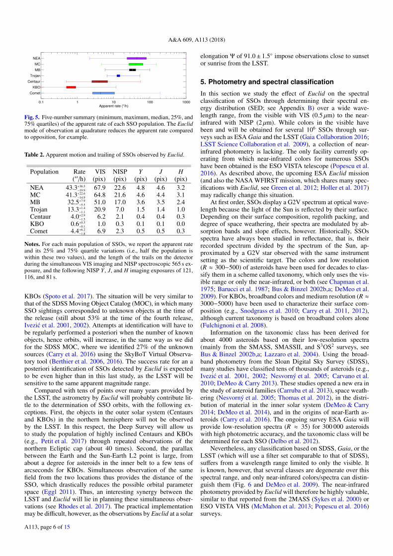
The real challenge of SSO observations with Euclid will be theastrometry and photometry of highly elongated sources (as indi-cated in Fig. 3). We present in Fig. 5 and Table 2 a summary ofthe apparent non-sidereal rate of the different SSO populations.With the exception of the most distant populations of KBOs,Centaurs, and comets, all SSOs will present rates above 10′′/h.This implies a motion of hundreds of pixels between the first andlast VIS frame. During a single exposure, each SSO will moveand produce a trailed signature, a streak, whose length will typ-ically range from 1 to 50 pixels for VIS. The situation will bemore favorable for NISP because of the shorter integration timesand larger pixel scale, and most SSOs will not trail, or will onlytrail across a few pixels (Table 2).
Some recent developments have been made to detect streaks,motivated by the optical detection and tracking of artificial satel-lites and debris on low orbits around the Earth. Dedicated im-age processing for trails can be set up to measure the astrometryand photometry of moving objects within a field of fixed stars,without an a priori knowledge of their apparent motion (e.g.,Virtanen et al. 2016). The success rate in detecting these trailshas been shown to reach up to 90%, even in the regime withlow signal-to-noise ratio (≈1). These algorithms are currently be-ing tested on simulated Euclid data of SSOs (M. Granvik, priv.comm.).
4. Source identification, astrometry, and dynamics
As established in Sect. 2, Euclid will observe about150 000 SSOs, even if its nominal survey avoids ecliptic lati-tudes below 15◦, with the notable exception of the calibrationfields (Fig. 1).
The design of the surveys, with hour-long sequences of ob-servation of each field, will preclude orbit determination fornewly discovered objects, however. This hour-long coverage isnevertheless sufficient to distinguish between NEAs, MBAs, and
A113, page 5 of 15
A&A 609, A113 (2018)
0.1 1 10 100 1000Apparent rate ("/h)
Comet
KBO
Centaur
Trojan
MB
MC
NEA
Fig. 5. Five-number summary (minimum, maximum, median, 25%, and75% quartiles) of the apparent rate of each SSO population. The Euclidmode of observation at quadrature reduces the apparent rate comparedto opposition, for example.
Table 2. Apparent motion and trailing of SSOs observed by Euclid.
Population Rate VIS NISP Y J H(′′/h) (pix) (pix) (pix) (pix) (pix)
NEA 43.3+36.5−19.9 67.9 22.6 4.8 4.6 3.2
MC 41.3+22.6−14.9 64.8 21.6 4.6 4.4 3.1
MB 32.5+7.9−5.5 51.0 17.0 3.6 3.5 2.4
Trojan 13.3+1.4−1.1 20.9 7.0 1.5 1.4 1.0
Centaur 4.0+2.9−1.5 6.2 2.1 0.4 0.4 0.3
KBO 0.6+0.3−0.1 1.0 0.3 0.1 0.1 0.0
Comet 4.4+6.2−1.8 6.9 2.3 0.5 0.5 0.3
Notes. For each main population of SSOs, we report the apparent rateand its 25% and 75% quartile variations (i.e., half the population iswithin these two values), and the length of the trails on the detectorduring the simultaneous VIS imaging and NISP spectroscopic 565 s ex-posure, and the following NISP Y , J, and H imaging exposures of 121,116, and 81 s.
KBOs (Spoto et al. 2017). The situation will be very similar tothat of the SDSS Moving Object Catalog (MOC), in which manySSO sightings corresponded to unknown objects at the time ofthe release (still about 53% at the time of the fourth release,Ivezic et al. 2001, 2002). Attempts at identification will have tobe regularly performed a posteriori when the number of knownobjects, hence orbits, will increase, in the same way as we didfor the SDSS MOC, where we identified 27% of the unknownsources (Carry et al. 2016) using the SkyBoT Virtual Observa-tory tool (Berthier et al. 2006, 2016). The success rate for an aposteriori identification of SSOs detected by Euclid is expectedto be even higher than in this last study, as the LSST will besensitive to the same apparent magnitude range.
Compared with tens of points over many years provided bythe LSST, the astrometry by Euclid will probably contribute lit-tle to the determination of SSO orbits, with the following ex-ceptions. First, the objects in the outer solar system (Centaursand KBOs) in the northern hemisphere will not be observedby the LSST. In this respect, the Deep Survey will allow usto study the population of highly inclined Centaurs and KBOs(e.g., Petit et al. 2017) through repeated observations of thenorthern Ecliptic cap (about 40 times). Second, the parallaxbetween the Earth and the Sun-Earth L2 point is large, fromabout a degree for asteroids in the inner belt to a few tens ofarcseconds for KBOs. Simultaneous observation of the samefield from the two locations thus provides the distance of theSSO, which drastically reduces the possible orbital parameterspace (Eggl 2011). Thus, an interesting synergy between theLSST and Euclid will lie in planning these simultaneous obser-vations (see Rhodes et al. 2017). The practical implementationmay be difficult, however, as the observations by Euclid at a solar
elongation Ψ of 91.0± 1.5◦ impose observations close to sunsetor sunrise from the LSST.
5. Photometry and spectral classification
In this section we study the effect of Euclid on the spectralclassification of SSOs through determining their spectral en-ergy distribution (SED; see Appendix B) over a wide wave-length range, from the visible with VIS (0.5 µm) to the near-infrared with NISP (2 µm). While colors in the visible havebeen and will be obtained for several 106 SSOs through sur-veys such as ESA Gaia and the LSST (Gaia Collaboration 2016;LSST Science Collaboration et al. 2009), a collection of near-infrared photometry is lacking. The only facility currently op-erating from which near-infrared colors for numerous SSOshave been obtained is the ESO VISTA telescope (Popescu et al.2016). As described above, the upcoming ESA Euclid mission(and also the NASA WFIRST mission, which shares many spec-ifications with Euclid, see Green et al. 2012; Holler et al. 2017)may radically change this situation.
At first order, SSOs display a G2V spectrum at optical wave-length because the light of the Sun is reflected by their surface.Depending on their surface composition, regolith packing, anddegree of space weathering, their spectra are modulated by ab-sorption bands and slope effects, however. Historically, SSOsspectra have always been studied in reflectance, that is, theirrecorded spectrum divided by the spectrum of the Sun, ap-proximated by a G2V star observed with the same instrumentsetting as the scientific target. The colors and low resolution(R ≈ 300−500) of asteroids have been used for decades to clas-sify them in a scheme called taxonomy, which only uses the vis-ible range or only the near-infrared, or both (see Chapman et al.1975; Barucci et al. 1987; Bus & Binzel 2002b,a; DeMeo et al.2009). For KBOs, broadband colors and medium resolution (R ≈3000−5000) have been used to characterize their surface com-position (e.g., Snodgrass et al. 2010; Carry et al. 2011, 2012),although current taxonomy is based on broadband colors alone(Fulchignoni et al. 2008).
Information on the taxonomic class has been derived forabout 4000 asteroids based on their low-resolution spectra(mainly from the SMASS, SMASSII, and S3OS2 surveys, seeBus & Binzel 2002b,a; Lazzaro et al. 2004). Using the broad-band photometry from the Sloan Digital Sky Survey (SDSS),many studies have classified tens of thousands of asteroids (e.g.,Ivezic et al. 2001, 2002; Nesvorný et al. 2005; Carvano et al.2010; DeMeo & Carry 2013). These studies opened a new era inthe study of asteroid families (Carruba et al. 2013), space weath-ering (Nesvorný et al. 2005; Thomas et al. 2012), in the distri-bution of material in the inner solar system (DeMeo & Carry2014; DeMeo et al. 2014), and in the origins of near-Earth as-teroids (Carry et al. 2016). The ongoing survey ESA Gaia willprovide low-resolution spectra (R ≈ 35) for 300 000 asteroidswith high photometric accuracy, and the taxonomic class will bedetermined for each SSO (Delbo et al. 2012).
Nevertheless, any classification based on SDSS, Gaia, or theLSST (which will use a filter set comparable to that of SDSS),suffers from a wavelength range limited to only the visible. Itis known, however, that several classes are degenerate over thisspectral range, and only near-infrared colors/spectra can distin-guish them (Fig. 6 and DeMeo et al. 2009). The near-infraredphotometry provided by Euclid will therefore be highly valuable,similar to that reported from the 2MASS (Sykes et al. 2000) orESO VISTA VHS (McMahon et al. 2013; Popescu et al. 2016)surveys.
A113, page 6 of 15

B. Carry: Solar system science with ESA Euclid
0.5 1.0 1.5 2.0Wavelength (µm)
0.0
0.5
1.0
1.5
2.0
Re
fle
cta
nce
(n
orm
aliz
ed
to
VIS
) A
D
S
V
VIS Y J H
blue grism red grism Euclid
YVISTA/UKIDSS JVISTA/UKIDSS HVISTA/UKIDSS KsVISTA/UKIDSS
uSDSS/LSST
gSDSS/LSST
rSDSS/LSST
iSDSS/LSST
zSDSS/LSST
BP RP Gaia
Fig. 6. Examples of asteroid classes (A, D, S, and V) that are de-generate over the visible wavelength range. For reference, the wave-length coverage of each photometric filter and grism on board Euclid isshown, together with the filter sets of SDSS and LSST (u, g, r, i, z;Ivezic et al. 2001), VISTA and UKIDSS (Y , J, H, Ks; Hewett et al.2006), and the Gaia blue and red photometers (BP, RP) that will pro-duce low-resolution spectra (resolving power of a few tens; Delbo et al.2012).
Wavelength (µm)
Reflecta
nce (
norm
aliz
ed to V
IS)
0.5
1.0
1.5
2.0
2.5
A−type
B−type
C−type
D−type
0.5
1.0
1.5
2.0
2.5
K−type
L−type
Q−type
S−type
0.5
1.0
1.5
2.0
2.5
T−type
V−type
X−type
0.5 1.0 1.5 2.0
0.5
1.0
1.5
2.0
2.5
BB−type
0.5 1.0 1.5 2.0
BR−type
0.5 1.0 1.5 2.0
IR−type
0.5 1.0 1.5 2.0
RR−type
0.0
0.2
0.4
0.6
0.8
1.0
VIS
Y JH
Filter transmission
Fig. 7. Eleven asteroid (A- to X-type) and four KBO (BB, BR, IR,RR) spectral classes considered here, converted into photometry for theclassification simulation (see text). The transmission curves of the VISand NISP filters are also plotted for reference.
To estimate the potential of the Euclid photometry for aspectral classification of asteroids, we simulated data using thevisible and near-infrared spectra of the 371 asteroids that wereused to create the Bus-DeMeo taxonomy (DeMeo et al. 2009),and of 43 KBOs with known taxonomy (Merlin et al. 2017). Weconverted their reflectance spectra into photometry (Fig. 7), tak-ing the reference VIS and NISP filter transmission curves2.
2 Available at the Geneva university Euclid pages.
0.4
0.6
0.8
1.0
1.2
1.4
Y−
H
A
B
C
D
K
L
Q
S TX
V
0.2 0.4 0.6 0.8Vis−Y
0.6
0.8
1.0
1.2
1.4
Vis
−J
A
B
C
D
K
L
Q
ST
X
V
0.6 0.8 1.0 1.2 1.4Vis−J
A
B
C
D
K
L
Q
S TX
V
A−types: 6
B−types: 4
C−types: 45
D−types: 16
K−types: 16
L−types: 22
Q−types: 8
S−types: 201
T−types: 4
X−types: 32
V−types: 17
Fig. 8. Classification results for the 371 asteroids from Bus-DeMeo tax-onomy, presented in three filter combinations: VIS-Y, VIS-J, and Y-H.Several extreme classes, such as A, B, D, V, and T, can be easily dis-carded thanks to the large wavelength coverage of Euclid.
One key aspect of the Euclid operations in determining theSSO colors is the repetition of the four-filter sequence during anhour. Thus, each filter will be bracketed by other filters in time.This will allow determining magnitude difference between eachpair of filters without the biases that are otherwise introduced bythe intrinsic variation of the target (Appendix B). For a detaileddiscussion of this effect, see Popescu et al. (2016).
For each class and filter combination, we computed the av-erage color, dispersion, and covariance. This allowed us to clas-sify objects based on their distance to all the class centers, nor-malized by the typical spread of the class (Pajuelo 2017). Thislearning sample is of course limited in number, and all classesare not evenly represented. It nevertheless allowed us to estimatethe Euclid capabilities by applying the classification scheme tothe same sample. This is presented in Fig. 8. The leverage pro-vided by the long wavelength coverage allowed us to clearlyidentify several classes: A, B, D, V, Q, and T (DeMeo et al.2009). The main classes in the asteroid belt, the C, S, and X(DeMeo & Carry 2014), are more clumped, and our capabili-ties to classify them will depend on the exact throughput of theoptical path of Euclid.
For KBOs, their spectral behavior from the blue-ish BB tothe extremely red RR will place them in these graphs along aline that extends from the C, T, and D types (whose colors areclose to those of the BB, BR, and IR classes). The RR typeswill be even farther from the central clump than the D types.Identifying the different KBO spectral classes should thereforebe straightforward with the filter set of Euclid.
In all cases, a spectral characterization using Euclid col-ors will benefit from the colors and spectra in the vis-ible observed by Gaia and the LSST (Delbo et al. 2012;LSST Science Collaboration et al. 2009), the visible albedo(from IRAS, AKARI, WISE, and Herschel observations; e.g.,Tedesco et al. 2002; Müller et al. 2009; Masiero et al. 2011;Usui et al. 2011), and solar phase function parameters (see
A113, page 7 of 15

A&A 609, A113 (2018)
0 20 40 60 80 100
0 20 40 60 80 100
Fraction of classification
Euclid c
lassific
ation
V
X
T
S
Q
L
K
D
C
B
A
S
S
S
K
X
L
C
Q
B
B
Fig. 9. Percentage of correct (solid bar) and compatible (open bar) clas-sification for each Bus-DeMeo taxonomic classes. The Euclid photom-etry alone allows to classify asteroids into 11 classes.
Oszkiewicz et al. 2012, for an example of using the phase func-tion for taxonomy). The success rate of a classification based onEuclid photometry therefore only represents a lower estimate.
We present in Fig. 9 the success rate of a classification of the371 asteroids from the Bus-DeMeo taxonomy. The classes aregenerally recovered with a success rate above 60%, and whenmisclassified, asteroids are sorted into spectrally similar (com-patible) classes with a success rate closer to 90%, except forthe C and X classes. We did not repeat the exercise for KBOsbecause the available sample is limited. Because their spectralclasses are very similar to those of the C, T, and D-type aster-oids, and because they are even redder, we expect that it will bestraightforward to identify them with the filter set of Euclid.
In summary, the VIS and NISP photometry that will be mea-sured by Euclid seems very promising to classify SSOs into theirhistorical spectral classes.
6. Near-infrared spectroscopy with NISP
Euclid will also acquire near-infrared low-resolution (resolvingpower of 380) spectra for many SSOs, down to mAB ≈ 21, whichis similar to the limiting magnitude of Gaia. Simultaneously tothe four VIS exposures, NISP will acquire four slitless spectraof the same FOV. In the Wide Survey, only the red grism (1.25to 1.85 µm) will be used, the usage of the blue grism (0.92 to1.25 µm) being limited to the Deep Survey. The red grism willcover typical absorption bands of volatile compounds (e.g., wa-ter or methane ices) such as are found on distant KBOs. Themain diagnostic features of asteroids (NEAs, MBAs) are locatedwithin the blue arm at 1 µm and at 2 µm, however, which is out-side the spectral range of the red grism.
Because there is no slit, many sources will be blended. Todecontaminate each slitless spectrum from surrounding sources,the exposures will be taken with three different grism orien-tations, 90◦ apart. For exposures whose spectral dispersion isaligned with the ecliptic, that is, which are parallel to the typ-ical SSO motion, each SSO will blend with itself. For the re-maining orientations, SSOs will often blend with backgroundsources, which degrades both spectra. This may be a problem forthe wide survey in its lowermost ecliptic latitude range, wheremany sources will be blended with G2V spectra from SSOs.
The apparent motion of outer SSOs being limited (Table 2),their spectra may be extracted by the Euclid consortium tools,which are designed to work on elongated sources (typically 1′′).Near-infrared spectra for thousands of Centaurs and KBOs couldthus be produced by Euclid. It may be challenging to extractthe spectra for objects in the inner solar system, and an in-depthassessment of the feasibility of such measurements is beyondthe scope of this paper. In both cases, these spectra will be verysimilar to the low-resolution spectra that were used to define thecurrent asteroid taxonomy (DeMeo et al. 2009) and diagnosticof the KBO class as defined by (Fulchignoni et al. 2008).
7. Multiplicity and activity of SSOs
With a very stable PSF and a pixel scale of 0.1′′ and 0.3′′ forVIS and NISP, which is close to the diffraction limit of Euclid,the source morphology can be studied. This is indeed one of themain goals of the cosmological survey (Laureijs et al. 2011). Wefirst assess how Euclid might detect satellites around SSOs, andthen consider their activity, that is, their dust trails.
7.1. Direct imaging of multiple systems with Euclid
In the two decades since the discovery of the first aster-oid satellite, Dactyl around (243) Ida, by the Galileo mission(Chapman et al. 1995), direct imaging has been the main sourceof discovery and characterization of satellites around largeSSOs in the main belt (e.g., Merline et al. 1999; Berthier et al.2014), among Jupiter Trojans (Marchis et al. 2006, 2014), andKBOs (e.g., Brown et al. 2005, 2006, 2010; Carry et al. 2011;Fraser et al. 2017). This is particularly evident for KBOs, forwhich 65 of the 80 known binary systems where discovered bythe Hubble Space Telescope, and the other 14 by large ground-based telescopes, often supported by adaptive optics (see, e.g.,Parker et al. 2011; Johnston 2015; Margot et al. 2015). The sit-uation is different for NEAs and small MBAs, for which mostdiscoveries and follow-up observations were made with opti-cal light curves and radar echoes (e.g., Pravec & Harris 2007;Pravec et al. 2012; Fang et al. 2011; Brozovic et al. 2011).
To estimate the capabilities of Euclid to angularly resolvea multiple system, we used the compilation of system parame-ters by Johnston (2015). We computed the magnitude differencebetween components ∆m from their diameter ratio, and their typ-ical separation Θ from the ratio of the binary system semimajoraxis to its heliocentric semimajor axis (Table 3).
The angular resolution of Euclid will thus allow us to detectsatellites of KBOs and large MBAs, but not those around NEAs,MCs, and small MBAs. The case of KBOs is straightforward,owing to the very little smearing of their PSF from their apparentmotion (Table 2). Based on the expected number of observationsof KBOs (Table 1) and their binarity fraction, Euclid is expectedto observe 300± 200 multiple KBO systems, which is a four-foldincrease.
The case of MBAs is more complex. First, there are only25 large MBAs with an inclination higher than 15◦, which willmake them potentially observable by Euclid. Second, the frac-tion and properties of multiple systems for MBAs with a diam-eter of between 10 and 100 km is terra incognita. The reasonare observational biases: detection by light curves is more ef-ficient on close-by components, and direct imaging, especiallyfrom ground-based telescopes using adaptive optics, focused onbright, hence large, primaries. If most binaries around smallasteroids (D < 10 km) are likely formed by rotational fission
A113, page 8 of 15
B. Carry: Solar system science with ESA Euclid
Table 3. Typical magnitude difference (∆m) and angular separation (Θ)between components of multiple SSO systems.
Population ∆m Θ f(mag) (′′) (%)
NEA and MC 1.8+2.0−1.8 0.01+0.01
−0.01 15 ± 5
MBA (D < 10 km) 2.5+0.9−0.9 0.01+0.01
−0.01 15 ± 5
MBA (D > 100 km) 5.4+2.7−2.7 0.30+0.25
−0.25 3 ± 2
KBO 1.5+2.0−1.5 0.43+0.60
−0.43 6 ± 4
Notes. NEA and MCs share similar characteristics, and so do largeMBAs and Trojans. We split MBAs into two categories according to thediameter D of the main component. Estimates on the binary frequencyin each populations are based on the reviews by Noll et al. (2008) andMargot et al. (2015). We only consider high-inclination KBOs here be-cause the binary fraction in the cold belt is closer to 30% (Fraser et al.2017).
caused by YORP spin-up (Walsh et al. 2008; Pravec et al. 2010;Walsh & Jacobson 2015), satellites of larger bodies are the resultof reaccumulation of ejecta material after impacts (Michel et al.2001; Durda et al. 2004). Some satellites around medium-sizedMBAs are therefore to be expected, but with unknown frequency.Considering a ratio of ≈5 between the semimajor axis of binarysystem and the diameter of the main component (typical of largeMBAs; see Margot et al. 2015) and the size distribution of high-inclination MBAs, only a handful of potential systems wouldhave separations that are angularly resolvable by Euclid. Finally,the apparent motion of MBAs implies highly elongated PSFs,which diminishes the fraction of detectable systems even further.
For these reasons, Euclid will contribute little if anything atall to the characterization of multiple systems among asteroids.The prospects for discovering KBO binaries are very promising,however.
7.2. Detection of activity
The distinction between comets and other types of small bodiesin our solar system is by convention based on the detection ofactivity, that is, of unbound atmosphere that is also called coma.Comets cannot be distinguished based only on their orbital ele-ments (Fig. A.1). The picture was blurred further with the dis-covery of comae around Centaurs and even MBAs, which arecalled active asteroids (see Jewitt 2009; Jewitt et al. 2015, forreviews).
The cometary-like behavior of these objects was discoveredeither by sudden surges in magnitude or by diffuse non-point-like emission around them. There are currently 18 known ac-tive asteroids and 12 known active Centaurs, corresponding to25 ppm and 13% of their host populations, respectively. Theproperty of the observed comae is typically 1 to 5 mag fainterthan the nucleus within a 3′′ radius (although this large aperturewas chosen to avoid contamination from the nucleus PSF, whichextended to about 2′′ due to atmospheric seeing, Jewitt 2009).
With much higher angular resolution and its very stable PSFas required for its primary science goal (Laureijs et al. 2011),Euclid has the capability of detecting activity like this. Based onthe expected number of observations (Table 1) and on the afore-mentioned fraction of observed activity, Euclid may observe sev-eral active asteroids and about 300+300
−200 active Centaurs. As inthe case of multiple systems, however, the detection capability
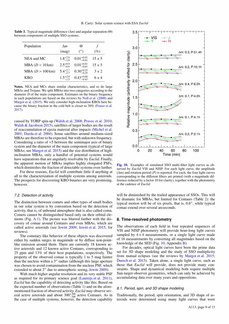
Fig. 10. Examples of simulated SSO multi-filter light curves as ob-served by Euclid VIS and NISP. For each light curve, the amplitude(∆m) and rotation period (P) is reported. For each, the four light curvescorresponding to the different filters are printed (with a magnitude dif-ference reduced by a factor 10 for clarity), together with the photometryat the cadence of Euclid.
will be diminished by the trailed appearance of SSOs. This willbe dramatic for MBAs, but limited for Centaurs (Table 2): thetypical motion will be of six pixels, that is, 0.6′′, while typicalcomae extend over several arcseconds.
8. Time-resolved photometry
The observations of each field in four repeated sequences ofVIS and NISP photometry will provide hour-long light curvessampled by 4× 4 measurements, or a single light curve madeof 16 measurements by converting all magnitudes based on theknowledge of the SED (Fig. 10, Appendix B).
For decades, optical light curves have been the prime dataset for 3D shape modeling and the study of SSO multiplicityfrom mutual eclipses (see the reviews by Margot et al. 2015;Durech et al. 2015). Taken alone, a single light curve, such asthose that Euclid will provide, does not provide many con-straints. Shape and dynamical modeling both require multipleSun-target-observer geometries, which can only be achieved byaccumulating data over many years and oppositions.
8.1. Period, spin, and 3D shape modeling
Traditionally, the period, spin orientation, and 3D shape of as-teroids were determined using many light curves that were
A113, page 9 of 15

A&A 609, A113 (2018)
Fig. 11. Cumulative distribution of the rotation fraction covered by onehour of observations, computed on the 5759 entries with a quality code 2or 3 from the Planetary Data System archive (Harris et al. 2017), and the25 comets from Samarasinha et al. (2004) and Lowry et al. (2012).
taken over several apparitions (e.g., Kaasalainen & Torppa2001; Kaasalainen et al. 2001). It has been show later on thatphotometry measurements, sparse in time3, convey the same in-formation and can be use alone or in combination with denselight curves (Kaasalainen 2004). Large surveys such as Gaia andthe LSST will deliver sparse photometry for several 105−6 SSOs(Mignard et al. 2007; LSST Science Collaboration et al. 2009).
In assessing the effect of PanSTARRS and Gaia dataon shape modeling, Durech et al. (2005) and Hanuš & Durech(2012) showed, however, that searching for the rotation periodwith sparse photometry alone may result in many ambiguous so-lutions. The addition of a single dense light curve often removesmany aliases and harmonics in a periodogram and removes theambiguous solutions; the effect of the single light curve dependson the fraction of the period it covers (J. Durech, pers. comm.).
The rotation periods of SSOs range from a few minutesto several hundred hours. The bulk of the distribution, how-ever, is confined to between 2.5 h (which is called the spin bar-rier, see e.g., Scheeres et al. 2015) and 10–15 h. This impliesthat Euclid light curves will typically cover between 5–10 and40% of the SSO rotation periods (Fig. 11). Euclid light curveswill cover more than a quarter of the rotation (the maximumchange in geometry over a rotation, used here as a baseline) for35% of NEAs, 28% of MCs, and 16% of MBAs, and only ahandful of outer SSOs. The hour-long light curves provided byEuclid will thus be valuable for 3D shape modeling of thousandsof asteroids (5.25+3.50
−2.10 × 10³ NEAs, 3.36+4.76−2.24 × 10³ MCS, and
1.55+0.40−0.35 × 10⁴ MBAs).
8.2. Mutual events and multiplicity
Binary asteroids represent about 15± 5% of the population ofNEAs that are larger than 300 m (Sect. 7; Pravec et al. 2006), anda similar fraction is expected among MCs and MBAs with a di-ameter smaller than 10 km (Table 3; Margot et al. 2015). Most ofthese multiple systems were discovered by light-curve observa-tions that recorded mutual eclipsing and occulting events (140 ofthe 205 binary asteroid systems known to date, the remaining aremostly binary NEAs discovered by radar echoes; see Johnston2015).
These systems have orbital periods of 24 ± 10 h and a di-ameter ratio of 0.33 ± 0.17, which implies a magnitude dropof 0.11+0.13
−0.08 during mutual eclipses and occultations (computed
3 Light curves whose sampling is typically longer than the period arecalled sparse photometry, as opposed to dense light curves, whose pe-riod is sampled by many measurements (see, e.g., Hanuš et al. 2016).
from the compilation of binary system properties by Johnston2015). The hour-long light curves provided by Euclid will thustypically cover 4+3
−1% of the orbital period. When we considerthat the systems are in mutual events for about 20% of the or-bital period at the high phase angle probed by Euclid (e.g.,Pravec et al. 2006; Carry et al. 2015), there is a correspond-ing probability of ≈(5± 2)% to witness mutual events. Hence,Euclid could record mutual events for 900+700
−450 NEAs, MCs, andMBAs, which will help to characterize these systems in combi-nation with other photometric data sets, such as those providedby Gaia and the LSST.
9. Conclusion
We have explored how the ESA mission Euclid might contributeto solar system science. The operation mode of Euclid is bychance well designed for the detection and identification of mov-ing objects. The deep limiting magnitude (VAB ∼ 24.5) of Euclidand large survey coverage (even though low ecliptic latitudes areavoided) promise about 150 000 observations of SSOs in all dy-namical classes, from near-Earth asteroids to distant Kuiper-beltobjects, including comets.
The spectral coverage of Euclid photometry, from the visibleto the near-infrared, complements the spectroscopy and photom-etry obtained in the visible alone by Gaia and the LSST; thiswill allow a spectral classification. The hour-long sequence ofobservations can be used to constrain the rotation period, spinorientation, 3D shape, and multiplicity of SSOs when combinedwith the sparse photometry of Gaia and the LSST. The high an-gular resolution of Euclid is expected to allow the detection ofseveral hundreds of satellites around KBOs and activity for thesame number of Centaurs.
The exact number of observations of SSOs, the determina-tion of the astrometric, photometric, and spectroscopic precisionas a function of apparent magnitude and rate, and the details ofdata treatments will have to be refined when the instruments arefully characterized. The exploratory work presented here aims atmotivating further studies on each aspect of SSO observationsby Euclid.
In summary, against all odds, a survey explicitly avoidingthe ecliptic promises great scientific prospects for solar systemresearch, which could be delivered as Legacy Science for Euclid.A dedicated SSO processing is currently being developed withinthe framework of the Euclid data analysis pipeline. The maingoal of the mission will benefit from this addition through theidentification of blended sources (e.g., stars and galaxies) withSSOs.
Furthermore, any extension of the survey to lower latitudewould dramatically increase the figures reported here: there aretwice as many SSOs for every 3◦ closer to the ecliptic. Any ob-servation at low ecliptic latitude, such as calibration fields, dur-ing idle time of the main survey or after its completion, or dedi-cated to a solar system survey would provide thousands of SSOseach time, allowing us to study the already-known dark matterof our solar system: the low-albedo minor planets.
Acknowledgements. The present study made a heavy use of the VirtualObservatory tools SkyBoT4 (Berthier et al. 2006, 2016), SkyBoT 3D5
(Berthier et al. 2008), TOPCAT6, and STILTS7 (Taylor 2005). Thanks to thedevelopers for their development and reaction to my requests, in particular,
4 SkyBoT: http://vo.imcce.fr/webservices/skybot/5 SkyBoT 3D: http://vo.imcce.fr/webservices/skybot3d/6 TOPCAT: http://www.star.bris.ac.uk/~mbt/topcat/7 STILTS: http://www.star.bris.ac.uk/~mbt/stilts/
A113, page 10 of 15

B. Carry: Solar system science with ESA Euclid
J. Berthier. The present article benefits from many discussions and commentsI received, and I would like to thank L. Maquet and C. Snodgrass for our dis-cussions regarding comet properties, the ESA Euclid group at ESAC B. Altieri,P. Gomez, H. Bouy, and R. Vavrek for our discussions on Euclid and SSO, in par-ticular P. Gomez for sharing the Reference Survey with me. Of course, I wouldnot have had these motivating experiences without the support of the ESAC fac-ulty (ESAC-410/2016). Thanks to F. Merlin for creating and sharing the KBOaverage spectra for this study. Thanks also to R. Laureijs and T. Müller for theirconstructive comments on an early version of this article, and to S. Paltani andR. Pello for providing the transmission curves of the VIS and NISP filters.
ReferencesAbazajian, K., Adelman-McCarthy, J. K., Agüeros, M. A., et al. 2003, AJ, 126,
2081Adams, E. R., Gulbis, A. A. S., Elliot, J. L., et al. 2014, AJ, 148, 55Bannister, M. T., Kavelaars, J. J., Petit, J.-M., et al. 2016, AJ, 152, 70Barucci, M. A., Capria, M. T., Coradini, A., & Fulchignoni, M. 1987, Icarus, 72,
304Bauer, J. M., Grav, T., Blauvelt, E., et al. 2013, ApJ, 773, 22Berthier, J., Vachier, F., Thuillot, W., et al. 2006, in Astronomical Data Analysis
Software and Systems XV, eds. C. Gabriel, C. Arviset, D. Ponz, & S. Enrique,ASP Conf. Ser., 351, 367
Berthier, J., Hestroffer, D., Carry, B., et al. 2008, LPI Contributions, 1405, 8374Berthier, J., Vachier, F., Marchis, F., Durech, J., & Carry, B. 2014, Icarus, 239,
118Berthier, J., Carry, B., Vachier, F., Eggl, S., & Santerne, A. 2016, MNRAS, 458,
3394Bowell, E., Hapke, B., Domingue, D., et al. 1989, Asteroids II, 524Bowell, E., Muinonen, K. O., & Wasserman, L. H. 1993, in Asteroids, Comets,
Meteors 1993, LPI Contributions, 810, 44Brown, M. E., Bouchez, A. H., Rabinowitz, D. L., et al. 2005, ApJ, 632, L45Brown, M. E., van Dam, M. A., Bouchez, A. H., et al. 2006, ApJ, 639, 43Brown, M. E., Ragozzine, D., Stansberry, J., & Fraser, W. C. 2010, AJ, 139, 2700Brozovic, M., Benner, L. A. M., Taylor, P. A., et al. 2011, Icarus, 216, 241Bus, S. J., & Binzel, R. P. 2002a, Icarus, 158, 146Bus, S. J., & Binzel, R. P. 2002b, Icarus, 158, 106Carruba, V., Domingos, R. C., Nesvorný, D., et al. 2013, MNRAS, 433, 2075Carry, B., Hestroffer, D., DeMeo, F. E., et al. 2011, A&A, 534, A115Carry, B., Snodgrass, C., Lacerda, P., Hainaut, O., & Dumas, C. 2012, A&A,
544, A137Carry, B., Matter, A., Scheirich, P., et al. 2015, Icarus, 248, 516Carry, B., Solano, E., Eggl, S., & DeMeo, F. E. 2016, Icarus, 268, 340Carvano, J. M., Hasselmann, H., Lazzaro, D., & Mothé-Diniz, T. 2010, A&A,
510, A43Chang, C.-K., Ip, W.-H., Lin, H.-W., et al. 2014, ApJ, 788, 17Chapman, C. R., Morrison, D., & Zellner, B. H. 1975, Icarus, 25, 104Chapman, C. R., Veverka, J., Thomas, P. C., et al. 1995, Nature, 374, 783Cropper, M., Pottinger, S., Niemi, S.-M., et al. 2014, in Space Telescopes and
Instrumentation 2014: Optical, Infrared, and Millimeter Wave, SPIE, 9143,91430J
Delbo, M., Gayon-Markt, J., Busso, G., et al. 2012, Planet. Space Sci., 73, 86DeMeo, F., & Carry, B. 2013, Icarus, 226, 723DeMeo, F. E., & Carry, B. 2014, Nature, 505, 629DeMeo, F. E., Binzel, R. P., Slivan, S. M., & Bus, S. J. 2009, Icarus, 202, 160DeMeo, F. E., Binzel, R. P., Carry, B., Polishook, D., & Moskovitz, N. A. 2014,
Icarus, 229, 392Dohnanyi, J. S. 1969, J. Geophys. Res., 74, 2531Durda, D. D., Bottke, W. F., Enke, B. L., et al. 2004, Icarus, 170, 243Durech, J., Grav, T., Jedicke, R., Denneau, L., & Kaasalainen, M. 2005, Earth
Moon Planets, 97, 179Durech, J., Carry, B., Delbo, M., Kaasalainen, M., & Viikinkoski, M. 2015,
Asteroid Models from Multiple Data Sources (Univ. Arizona Press), 183Eggl, S. 2011, Celes. Mech. Dyn. Astron., 109, 211Epchtein, N., de Batz, B., Copet, E., et al. 1994, Astrophys. Space Sci., 217, 3Fang, J., Margot, J.-L., Brozovic, M., et al. 2011, AJ, 141, 154Fraser, W. C., Bannister, M. T., Pike, R. E., et al. 2017, Nature Astron., 1, 0088Fulchignoni, M., Belskaya, I., Barucci, M. A., De Sanctis, M. C., &
Doressoundiram, A. 2008, The Solar System Beyond Neptune, 181Gaia Collaboration (Prusti, T., et al.) 2016, A&A, 595, A1Gladman, B., Marsden, B. G., & Vanlaerhoven, C. 2008, Nomenclature in the
Outer Solar System (Univ. Arizona Press), 43Gladman, B. J., Davis, D. R., Neese, C., et al. 2009, Icarus, 202, 104Gladman, B., Lawler, S. M., Petit, J.-M., et al. 2012, AJ, 144, 23Granvik, M., Morbidelli, A., Jedicke, R., et al. 2016, Nature, 530, 303Grav, T., Mainzer, A. K., Bauer, J., et al. 2011, AJ, 742, 40
Green, J., Schechter, P., Baltay, C., et al. 2012, Wide-Field InfraRed SurveyTelescope (WFIRST) Final Report, Tech. Rep.
Hanuš, J., & Durech, J. 2012, Planet. Space Sci., 73, 75Hanuš, J., Durech, J., Oszkiewicz, D. A., et al. 2016, A&A, 586, A108Harris, A. W., & D’Abramo, G. 2015, Icarus, 257, 302Harris, A. W., Warner, B. D., & Pravec, P. 2017, NASA Planetary Data SystemHewett, P. C., Warren, S. J., Leggett, S. K., & Hodgkin, S. T. 2006, MNRAS,
367, 454Holler, B. J., Milam, S. N., Bauer, J. M., et al. 2017, ArXiv e-prints
[arXiv:1709.02763]Ivezic, Ž., Tabachnik, S., Rafikov, R., et al. 2001, AJ, 122, 2749Ivezic, Ž., Lupton, R. H., Juric, M., et al. 2002, AJ, 124, 2943Jedicke, R., & Metcalfe, T. S. 1998, Icarus, 131, 245Jedicke, R., Larsen, J., & Spahr, T. 2002, Asteroids III, 71Jewitt, D. 2003, Earth Moon Planets, 92, 465Jewitt, D. 2009, AJ, 137, 4296Jewitt, D. C., Trujillo, C. A., & Luu, J. X. 2000, AJ, 120, 1140Jewitt, D., Hsieh, H., & Agarwal, J. 2015, The Active Asteroids (Univ. Arizona
Press), 221Johnston, W. 2015, Binary Minor Planets V8.0, NASA Planetary Data System,
eAR-A-COMPIL-5-BINMP-V8.0Kaasalainen, M. 2004, A&A, 422, L39Kaasalainen, M., & Torppa, J. 2001, Icarus, 153, 24Kaasalainen, M., Torppa, J., & Muinonen, K. 2001, Icarus, 153, 37Laureijs, R., Amiaux, J., Arduini, S., et al. 2011, ArXiv e-prints
[arXiv:1110.3193]Lazzaro, D., Angeli, C. A., Carvano, J. M., et al. 2004, Icarus, 172, 179Lowry, S., Duddy, S. R., Rozitis, B., et al. 2012, A&A, 548, A12LSST Science Collaboration, Abell, P. A., Allison, J., et al. 2009, ArXiv e-prints
[arXiv:0912.0201]Maciaszek, T., Ealet, A., Jahnke, K., et al. 2014, in Space Telescopes and
Instrumentation 2014: Optical, Infrared, and Millimeter Wave, SPIE, 9143,91430K
Mahlke, M., Bouy, H., Altieri, B., et al. 2017, A&A, in press,DOI: 10.1051/0004-6361/201730924
Mainzer, A., Grav, T., Masiero, J., et al. 2011, ApJ, 741, 90Marchis, F., Hestroffer, D., Descamps, P., et al. 2006, Nature, 439, 565Marchis, F., Durech, J., Castillo-Rogez, J., et al. 2014, ApJ, 783, L37Margot, J.-L., Pravec, P., Taylor, P., Carry, B., & Jacobson, S. 2015, Asteroid
Systems: Binaries, Triples, and Pairs, eds. P. Michel, F. E. DeMeo, & W. F.Bottke (Univ. Arizona Press), 355
Masiero, J. R., Mainzer, A. K., Grav, T., et al. 2011, ApJ, 741, 68McMahon, R. G., Banerji, M., Gonzalez, E., et al. 2013, The Messenger, 154, 35Merlin, F., Hromakina, T., Perna, D., Hong, M. J., & Alvarez-Candal, A. 2017,
A&A, 604, A86Merline, W. J., Close, L. M., Dumas, C., et al. 1999, Nature, 401, 565Michel, P., Benz, W., Tanga, P., & Richardson, D. C. 2001, Science, 294, 1696Mignard, F., Cellino, A., Muinonen, K., et al. 2007, Earth Moon and Planets,
101, 97Muinonen, K., Belskaya, I. N., Cellino, A., et al. 2010, Icarus, 209, 542Müller, T. G., Lellouch, E., Böhnhardt, H., et al. 2009, Earth Moon Planets, 105,
209Nesvorný, D., Jedicke, R., Whiteley, R. J., & Ivezic, Ž. 2005, Icarus, 173, 132Noll, K. S., Grundy, W. M., Chiang, E. I., Margot, J.-L., & Kern, S. D. 2008,
Binaries in the Kuiper Belt, eds. M. A. Barucci, H. Boehnhardt, D. P.Cruikshank, A. Morbidelli, & R. Dotson, 345
Oszkiewicz, D. A., Bowell, E., Wasserman, L. H., et al. 2012, Icarus, 219,283
Pajuelo, M. 2017, Ph.D. Thesis, Observatoire de ParisParker, A. H., Kavelaars, J. J., Petit, J.-M., et al. 2011, ApJ, 743, 1Petit, J.-M., Bannister, M. T., Alexandersen, M., et al. 2016, in AAS/Division for
Planetary Sciences Meeting Abstracts, 48, 120.16Petit, J.-M., Kavelaars, J. J., Gladman, B. J., et al. 2017, AJ, 153, 236Polishook, D., Ofek, E. O., Waszczak, A., et al. 2012, MNRAS, 421, 2094Popescu, M., Licandro, J., Morate, D., et al. 2016, A&A, 591, A115Pravec, P., & Harris, A. W. 2007, Icarus, 190, 250Pravec, P., Scheirich, P., Kušnirák, P., et al. 2006, Icarus, 181, 63Pravec, P., Vokrouhlický, D., Polishook, D., et al. 2010, Nature, 466, 1085Pravec, P., Scheirich, P., Vokrouhlický, D., et al. 2012, Icarus, 218, 125Rhodes, J., Nichol, B., Aubourg, E., et al. 2017Russell, C. T., Raymond, C. A., Coradini, A., et al. 2012, Science, 336, 684Samarasinha, N. H., Mueller, B. E. A., Belton, M. J. S., & Jorda, L. 2004,
Rotation of cometary nuclei (Univ. Arizona Press), 281Scheeres, D. J., Britt, D., Carry, B., & Holsapple, K. A. 2015, Asteroid Interiors
and Morphology, eds. P. Michel, F. E. DeMeo, & W. F. Bottke (Univ. ArizonaPress), 745
Shankman, C., Kavelaars, J., Gladman, B. J., et al. 2016, AJ, 151, 31Sierks, H., Lamy, P., Barbieri, C., et al. 2011, Science, 334, 487
A113, page 11 of 15

A&A 609, A113 (2018)
Skrutskie, M. F., Cutri, R. M., Stiening, R., et al. 2006, AJ, 131, 1163Snodgrass, C., Carry, B., Dumas, C., & Hainaut, O. R. 2010, A&A, 511, A72Snodgrass, C., Fitzsimmons, A., Lowry, S. C., & Weissman, P. 2011, MNRAS,
414, 458Spoto, F., Del Vigna, A., Milani, A., Tomei, G., & Tanga, P. 2017, A&A,
submittedSykes, M. V., Cutri, R. M., Fowler, J. W., et al. 2000, Icarus, 146, 161Szabó, G. M., Ivezic, Ž., Juric, M., Lupton, R., & Kiss, L. L. 2004, MNRAS,
348, 987Taylor, M. B. 2005, in Astronomical Data Analysis Software and Systems XIV,
eds. P. Shopbell, M. Britton, & R. Ebert, ASP Conf. Ser., 347, 29Tedesco, E. F., Noah, P. V., Noah, M. C., & Price, S. D. 2002, AJ, 123, 1056
Thomas, C. A., Trilling, D. E., & Rivkin, A. S. 2012, Icarus, 219, 505Usui, F., Kuroda, D., Müller, T. G., et al. 2011, PASJ, 63, 1117Veverka, J., Robinson, M., Thomas, P., et al. 2000, Science, 289, 2088Virtanen, J., Poikonen, J., Säntti, T., et al. 2016, Adv. Space Res., 57,
1607Volk, K., Murray-Clay, R., Gladman, B., et al. 2016, AJ, 152, 23Walsh, K. J., & Jacobson, S. A. 2015, Formation and Evolution of Binary
Asteroids, eds. P. Michel, F. E. DeMeo, & W. F. Bottke, 375Walsh, K. J., Richardson, D. C., & Michel, P. 2008, Nature, 454, 188Waszczak, A., Chang, C.-K., Ofek, E. O., et al. 2015, AJ, 150, 75Wiegert, P., Balam, D., Moss, A., et al. 2007, AJ, 133, 1609Yoshida, F., & Nakamura, T. 2005, AJ, 130, 2900
A113, page 12 of 15

B. Carry: Solar system science with ESA Euclid
Appendix A: Definition of small-body populations
We describe here the boundaries in orbital elements to define the population we used thoroughout the article. The boundaries forNEA classes are taken from Carry et al. (2016), and the boundary of the outer solar system is adopted from Gladman et al. (2008).
2:1
3:2
8:3
0.1 1.0 10 1000.0
0.2
0.4
0.6
0.8
1.0
Atiras Atens ApollosVulcanoids Centaurs Scattered-disk objects
Tro
jans
IMB
MM
BO
MB
Cyb
eles
Hild
as
Ecc
entr
icity
Semi-major axis (au)
Amors
Mars
-crosse
rs
H Mai
nIn
ner
Detached
Out
er
Classical belt
Resonant
Short-period CometsNear-Earth Asteroid
Main-belt Asteroid(NEA)(MBA)
Kuiper-belt Object (KBO)
♄☿ ♀ ♁ ♂ ♃ ♅ ♆
Fig. A.1. Different classes of SSOs used thoroughout the article. H stands for Hungarias, and IMB, MMB, and OMB for inner, middle, and outerbelt, respectively. Comet orbital elements formally overlap with other classes because their classification is based on the presence of a coma atshort heliocentric distance.
Table A.1. Definition of all the dynamical populations use here as a function of their semimajor axis, eccentricity, perihelion, and aphelion (usingthe definitions in Carry et al. 2016; Gladman et al. 2008).
Class Semimajor axis (au) Eccentricity Perihelion (au) Aphelion (au)min. max. min. max. min. max. min. max.
NEA – – – – – 1.300 – –Atira – a♁ – – – – – q♁Aten – a♁ – – – – q♁ –Apollo a♁ 4.600 – – – Q♁ – –Amor a♁ 4.600 – – Q♁ 1.300 – –
MC 1.300 4.600 – – 1.300 Q♂ – –MBA Q♂ 4.600 – – Q♂ – – –
Hungaria – J4:1 – – Q♂ – – –IMB J4:1 J3:1 – – Q♂ – – –MMB J3:1 J5:2 – – Q♂ – – –OMB J5:2 J2:1 – – Q♂ – – –Cybele J2:1 J5:3 – – Q♂ – – –Hilda J5:3 4.600 – – Q♂ – – –
Trojan 4.600 5.500 – – – – – –Centaur 5.500 a[ – – – – – –KBO a[ – – – – – – –
SDO a[ – – – – 37.037 – –Detached a[ – 0.24 – 37.037 – – –ICB 37.037 N2:3 – 0.24 37.037 – – –MCB N2:3 N1:2 – 0.24 37.037 – – –OCB N1:2 – – 0.24 37.037 – – –
Notes. See Fig. A.1 for the distribution of these populations in the semimajor axis – eccentricity orbital element space. The numerical value of thesemimajor axes a, perihelion q, aphelion Q, and mean-motion resonances (indices i: j) are for the Earth a♁, q♁, and Q♁ at 1.0, 0.983, and 1.017 AU;for Mars Q♂ at 1.666 AU; for Jupiter J4:1, J3:1, J5:2, J2:1, and J5:3 at 2.06, 2.5, 2.87, 3.27, 3.7 AU; and for Neptune a[, N2:3, and N1:2 at 30.07, 47.7,and 39.4 AU. The somewhat arbitrary limit of 37.037 AU corresponds to the innermost perihelion that is accessible to detached KBOs (semimajoraxis of N1:2 and eccentricity of 0.24).
A113, page 13 of 15

A&A 609, A113 (2018)
Appendix B: Euclid colors and SSO light curves
Owing to the ever-changing Sun-SSO-observer geometry andthe rotating irregular shape of SSOs, the apparent magnitudeof SSOs is constantly changing. Magnitude variations in multi-filter time series are thus a mixture of low-frequency geometricevolution, high-frequency shape-related variability, and intrinsicsurface colors.
The slow geometric evolution can easily be taken into ac-count (Eq. (1)), but we need to separate the intrinsic surface col-ors from the shape-related variability to build the SED (Sect. 5)and to obtain a dense light curve (Sect. 8). Often, only the sim-plistic approach of taking the pair of filters closest in time canbe used to determine the color (e.g., Popescu et al. 2016), whilehoping the shape-related variability will not affect the color mea-surements (Fig. 10, Szabó et al. 2004).
The sequence of observations by Euclid in four repeatedblocks, each containing all four filters (Fig. 2), allows a moresubtle approach, however. For any given color, that is, for eachfilter pair, each filter will be bracketed in time three times by theother filter. The reference magnitudes provided by the bracket-ing filter allow us to estimate the magnitude at the observing timeof the other filter. For instance, to determine the (VIS-Y) index,we can use the first two measurements in VIS to estimate theVIS magnitude at the time the Y filter was acquired (by simplelinear interpolation for instance). This corrects, although onlypartially, for the shape-related variability. Hence, any colors willbe evaluated six times over an hour, although not entirely inde-pendently each time.
The only notable assumption here is that the SED is constantover rotation, meaning that the surface composition and proper-ties are homogeneous on the surface, which is a soft assumptionbased on the history of spacecraft rendezvous with asteroids (i.e.,Eros, Gaspra, Itokawa, Mathilde, Ida, Šteins, Lutetia, and Ceres,with the only exception of the Vesta, see e.g., Veverka et al.2000; Sierks et al. 2011; Russell et al. 2012).
We tested this approach by simulating observation sequencesby Euclid. For each of the 371 asteroids of the DeMeo et al.(2009), we simulated 800 light curves made of Fourier seriesof the second order, with random coefficients to produce a lightcurve amplitude between 0 and 1.6 mag and a random rotationperiod between 1 and 200 h. These ≈300 000 light curves spanthe observed range of amplitude and period parameter space, es-timated from the 5759 entries with a quality code 2 or 3 from the
Planetary Data System archive (Fig. B.1; Harris et al. 2017). Welimited the simulation to second-order Fourier series as denselight curves for about a thousand asteroids from the PalomarTransient Factory showed that is was sufficient to reproducemost asteroid light curves (Polishook et al. 2012; Chang et al.2014; Waszczak et al. 2015). For each light curve, we deter-mined the 4× 4 apparent magnitude measurements using thedefinition of the observing sequence of Euclid (Fig. 2) and theSSO color (from Sect. 5), and we added a random Gaussian noiseof 0.02 mag.
We then analyzed these 4× 4 measurements with the methoddescribed above. For each SSO and each light curve, we deter-mined all the colors (VIS-Y, VIS-J, VIS-H, Y-J, Y-H, and J-H)and compared them with the input of the simulation, hereaftercalled the residuals. For each color, we also recorded the esti-mate dispersion.
The accuracy on each color was found to be at the level ofthe single measurement uncertainty (Fig. B.1). This is due to theavailability of multiple estimates of each color, which improvesthe resulting signal-to-noise ratio. The residuals are found tobe very close to zero: offsets below the millimagnitude (mmag)with a standard deviation below 0.01, that is, smaller than in-dividual measurement uncertainty (about a factor of five). Werepeated the analysis with higher levels of Gaussian noise onindividual measurements (0.05 and 0.10 mag, the latter corre-sponding to the expected precision at the limiting magnitudeof Euclid), adding 600 000 simulated light curves to the exer-cise, and found similar results: the color uncertainty remains atthe level of the uncertainty on individual measurement and theresiduals remain close to zero, with a dispersion following theindividual measurement uncertainty reduced by a factor of aboutfive. The colors determined with this technique are therefore pre-cise and reliable.
The processing described here is a simple demonstration thatthe SED can be precisely determined from Euclid multi-filtertime series. As a corollary, a single light curve of 16 measure-ments can be reconstructed from the 4× 4 measurements. Thesewill be the root of the spectral classification (Sect. 5) and time-resolved photometry analysis (Sect. 8). The technique will befurther refined for the data processing: we considered here eachcolor, that is, each pair of filters, independently. No attempt fora multi-pair analysis was made for this simple demonstration ofthe technique, while a combined analysis is expected to reducethe residuals, that is, potential biases, even more.
A113, page 14 of 15

B. Carry: Solar system science with ESA Euclid
Fig. B.1. Left: distribution of the dispersion of color measurement in period-amplitude space. The white contours represent the regions encompass-ing 50% and 99% of the population with known rotation period and amplitude, respectively. The largest uncertainties are found for high-amplitudeshort rotation-period light curves, which is outside the typical space sampled by SSOs. Right: distribution of the dispersion and residuals of colordetermination in VIS-Y, VIS-J, and VIS-H colors (the remaining colors are a combination of these three). The dispersion is typically at the levelof the individual measurement uncertainty (here 0.020 mag). Residuals are much smaller, close to zero, and with a dispersion below 0.01 mag.
A113, page 15 of 15