SMOOTH OPTIMIZATION APPROACH FOR SPARSE COVARIANCE …people.math.sfu.ca/~zhaosong/ResearchPapers/smoothcovsel.pdf · SMOOTH OPTIMIZATION APPROACH FOR SPARSE COVARIANCE SELECTION

SIAM J. OPTIM. c© 2009 Society for Industrial and Applied MathematicsVol. 19, No. 4, pp. 1807–1827

SMOOTH OPTIMIZATION APPROACH FOR SPARSECOVARIANCE SELECTION∗

ZHAOSONG LU†

Abstract. In this paper we first study a smooth optimization approach for solving a class ofnonsmooth strictly concave maximization problems whose objective functions admit smooth con-vex minimization reformulations. In particular, we apply Nesterov’s smooth optimization technique[Y. E. Nesterov, Dokl. Akad. Nauk SSSR, 269 (1983), pp. 543–547; Y. E. Nesterov, Math. Program-ming, 103 (2005), pp. 127–152] to their dual counterparts that are smooth convex problems. It isshown that the resulting approach has O(1/

√ε) iteration complexity for finding an ε-optimal solution

to both primal and dual problems. We then discuss the application of this approach to sparse covari-ance selection that is approximately solved as an l1-norm penalized maximum likelihood estimationproblem, and also propose a variant of this approach which has substantially outperformed the latterone in our computational experiments. We finally compare the performance of these approacheswith other first-order methods, namely, Nesterov’s O(1/ε) smooth approximation scheme and block-coordinate descent method studied in [A. d’Aspremont, O. Banerjee, and L. El Ghaoui, SIAM J.Matrix Anal. Appl., 30 (2008), pp. 56–66; J. Friedman, T. Hastie, and R. Tibshirani, Biostatistics,9 (2008), pp. 432–441] for sparse covariance selection on a set of randomly generated instances. Itshows that our smooth optimization approach substantially outperforms the first method above, andmoreover, its variant substantially outperforms both methods above.

Key words. sparse covariance selection, nonsmooth strictly concave maximization, smoothminimization

AMS subject classifications. 90C22, 90C25, 90C47, 65K05, 62J10

DOI. 10.1137/070695915

1. Introduction. In [19, 21], Nesterov proposed an efficient smooth optimiza-tion method for solving convex programming problems of the form

(1) min{f(u) : u ∈ U},

where f is a convex function with Lipschitz continuous gradient, and U is a closed con-vex set. It is shown that his method has O(1/

√ε) iteration complexity bound, where

ε > 0 is the absolute precision of the final objective function value. A proximal-point-type algorithm for (1) having the same complexity as above has also been proposedmore recently by Auslender and Teboulle [2].

Motivated by [10], we are particularly interested in studying the use of a smoothoptimization approach for solving a class of nonsmooth strictly concave maximizationproblems whose objective functions admit smooth convex minimization reformulationsin this paper. Our key idea is to apply Nesterov’s smooth optimization technique[19, 21] to their dual counterparts that are smooth convex problems. It is shown thatthe resulting approach has O(1/

√ε) iteration complexity for finding an ε-optimal

solution to both primal and dual problems.One interesting application of the above approach is for sparse covariance se-

lection. Given a set of random variables with Gaussian distribution for which the

∗Received by the editors June 30, 2007; accepted for publication (in revised form) October 3,2008; published electronically February 20, 2009.

http://www.siam.org/journals/siopt/19-4/69591.html†Department of Mathematics, Simon Fraser University, Burnaby, BC, V5A 1S6, Canada (zhaosong

@sfu.ca). This author was supported in part by NSERC Discovery Grant and SFU President’sResearch Grant.

1807

1808 ZHAOSONG LU

true covariance matrix is unknown, covariance selection is a procedure used to esti-mate true covariance from a sample covariance matrix by maximizing its likelihoodwhile imposing a certain sparsity on the inverse of the covariance estimation (e.g., see[11]). Therefore, it can be applied to determine a robust estimate of the true vari-ance matrix, and simultaneously to discover the sparse structure in the underlyingmodel. Despite its popularity in numerous real-world applications (e.g., see [3, 10, 25]and the references therein), sparse covariance selection itself is a challenging NP-hardcombinatorial optimization problem. By an argument that is often used in regres-sion techniques such as LASSO [23], Yuan and Lin [25] and d’Aspremont et al. [10](see also [3]) showed that it can be approximately solved as an l1-norm penalizedmaximum likelihood estimation problem. Moreover, the authors of [10] studied twoefficient first-order methods for solving this problem, that is, Nesterov’s smooth ap-proximation scheme and block-coordinate descent method. It was shown in [10] thattheir first method has O(1/ε) iteration complexity for finding an ε-optimal solution.For their second method, each iterate requires solving a box constrained quadraticprogramming, and it has a local linear convergence rate. However, its global iterationcomplexity for finding an ε-optimal solution is theoretically unknown. After the firstrelease of our paper, Friedman, Hastie, and Tibshirani [16] studied a slight variantof the block-coordinate descent method proposed in [10]. At each iteration of theirmethod, a coordinate descent approach is applied to solve a lasso (l1-regularized)least-squares problem, which is the dual of the box constrained quadratic program-ming appearing in the block-coordinate descent method [10]. In contrast with thesemethods, the smooth optimization approach proposed in this paper has a more at-tractive iteration complexity that is O(1/

√ε) for finding an ε-optimal solution. In

addition, we propose a variant of the smooth optimization approach which has sub-stantially outperformed the latter one in our computational experiments. We alsocompare the performance of our approaches with their methods for sparse covarianceselection on a set of randomly generated instances. It shows that our smooth opti-mization approach substantially outperforms their first method above (i.e., Nesterov’ssmooth approximation scheme) and, moreover, its variant substantially outperformstheir methods [10, 16] mentioned above.

The paper is organized as follows. In section 2, we introduce a class of nonsmoothconcave maximization problems in which we are interested and propose a smooth op-timization approach to them. In section 3, we briefly introduce sparse covarianceselection and show that it can be approximately solved as an l1-norm penalized max-imum likelihood estimation problem. We also discuss the application of the smoothoptimization approach for solving this problem and propose a variant of this approach.In section 4, we compare the performance of our smooth optimization approach andits variant with two other first-order methods studied in [10, 16] for sparse covari-ance selection on a set of randomly generated instances. Finally, we present someconcluding remarks in section 5.

1.1. Notation. In this paper, all vector spaces are assumed to be finite-dimen-sional. The space of symmetric n × n matrices will be denoted by Sn. If X ∈ Sn ispositive semidefinite, we write X � 0. Also, we write X � Y to mean Y − X � 0.The cone of positive semidefinite (resp., definite) matrices is denoted by Sn

+ (resp.,Sn

++). Given matrices X and Y in �p×q, the standard inner product is definedby 〈X,Y 〉 := Tr(XY T ), where Tr(·) denotes the trace of a matrix. ‖ · ‖ denotesthe Euclidean norm and its associated operator norm unless it is explicitly statedotherwise. The Frobenius norm of a real matrix X is defined as ‖X‖F :=

√Tr(XXT ).

SMOOTH OPTIMIZATION FOR SPARSE COVARIANCE SELECTION 1809

We denote by e the vector of all ones, and by I the identity matrix. Their dimensionsshould be clear from the context. For a real matrix X, we denote by Card(X) thecardinality of X, that is, the number of nonzero entries of X, and denote by |X|the absolute value of X, that is, |X|ij = |Xij | for all i, j. The determinant andthe minimal (resp., maximal) eigenvalue of a real symmetric matrix X are denotedby detX and λmin(X) (resp., λmax(X)), respectively. For an n-dimensional vector w,diag(w) denotes the diagonal matrix whose ith diagonal element is wi for i = 1, . . . , n.We denote by Z+ the set of all nonnegative integers.

Let the space F be endowed with an arbitrary norm ‖ · ‖. The dual space of F ,denoted by F∗, is the normed real vector space consisting of all linear functionals ofs : F → �, endowed with the dual norm ‖ · ‖∗ defined as

‖s‖∗ := maxu

{〈s, u〉 : ‖u‖ ≤ 1} ∀s ∈ F∗,

where 〈s, u〉 := s(u) is the value of the linear functional s at u. Finally, given anoperator A : F → F∗, we define

A[H,H] := 〈AH,H〉

for any H ∈ F .

2. Smooth optimization approach. In this section, we consider a class ofconcave nonsmooth maximization problems:

(2) maxx∈X

{g(x) := minu∈U

φ(x, u)},

where X and U are nonempty convex compact sets in finite-dimensional real vectorspaces E and F , respectively, and φ(x, u) : X×U → � is a continuous function whichis strictly concave in x ∈ X for every fixed u ∈ U , and convex differentiable in u ∈ Ufor every fixed x ∈ X. Therefore, for any u ∈ U , the function

(3) f(u) := maxx∈X

φ(x, u)

is well-defined. We also easily conclude that f(u) is convex differentiable on U , andits gradient is given by

(4) ∇f(u) = ∇uφ(x(u), u) ∀u ∈ U,

where x(u) denotes the unique solution of (3).Let the space F be endowed with an arbitrary norm ‖ · ‖. We further assume

that ∇f(u) is Lipschitz continuous on U with respect to ‖ · ‖, i.e., there exists someL > 0 such that

‖∇f(u) −∇f(u)‖∗ ≤ L‖u− u‖ ∀u, u ∈ U.

Under the above assumptions, we easily observe that (i) problem (2) and its dual,that is,

(5) minu

{f(u) : u ∈ U},

are both solvable and have the same optimal value; and (ii) the dual problem (5) canbe suitably solved by Nesterov’s smooth minimization approach [19, 21].

1810 ZHAOSONG LU

Denote by d(u) a prox-function of the set U . We assume that d(u) is continuousand strongly convex on U with modulus σ > 0. Let u0 be the center of the set Udefined as

(6) u0 = arg min{d(u) : u ∈ U}.

Without loss of generality assume that d(u0) = 0. We now describe Nesterov’s smoothminimization approach [19, 21] for solving the dual problem (5), and we will showthat it simultaneously solves the nonsmooth concave maximization problem (2).

Smooth minimization algorithm.

Let u0 ∈ U be given in (6). Set x−1 = 0 and k = 0.(1) Compute ∇f(uk) and x(uk). Set xk = k

k+2xk−1 + 2k+2x(uk).

(2) Find usdk ∈ Argmin

{〈∇f(uk), u− uk〉 + L

2 ‖u− uk‖2 : u ∈ U}.

(3) Find uagk = argmin

{Lσ d(u) +

∑ki=0

i+12 [f(ui) + 〈∇f(ui), u− ui〉] : u ∈ U

}.

(4) Set uk+1 = 2k+3u

agk + k+1

k+3usdk .

(5) Set k ← k + 1 and go to step 1.endThe following property of the above algorithm is established in Theorem 2 of

Nesterov [21].Theorem 2.1. Let the sequence {(uk, u

sdk )}∞k=0 ⊆ U × U be generated by the

smooth minimization algorithm. Then for any k ≥ 0 we have(7)

(k + 1)(k + 2)

4f(usd

k ) ≤ min

{L

σd(u) +

k∑i=0

i + 1

2[f(ui) + 〈∇f(ui), u− ui〉] : u ∈ U

}.

We are ready to establish the main convergence result of the smooth minimizationalgorithm for solving the nonsmooth concave maximization problem (2) and its dual(5). Its proof is a generalization of the one given in a more special context in [21].

Theorem 2.2. After k iterations, the smooth minimization algorithm generatesa pair of approximate solutions (usd

k , xk) to problem (2) and its dual (5), respectively,which satisfy the following inequality:

(8) 0 ≤ f(usdk ) − g(xk) ≤

4LD

σ(k + 1)(k + 2).

Thus if the termination criterion f(usdk ) − g(xk) ≤ ε is applied, the iteration com-

plexity of finding an ε-optimal solution to problem (2) and its dual (5) by the smoothminimization algorithm does not exceed 2

√LD/(σε), where

(9) D = max{d(u) : u ∈ U}.

Proof. In view of (3), (4), and the notation x(u), we have

(10) f(ui) + 〈∇f(ui), u− ui〉 = φ(x(ui), ui) + 〈∇uφ(x(ui), ui), u− ui〉.

Invoking the fact that the function φ(x, ·) is convex on U for every fixed x ∈ X, weobtain

φ(x(ui), ui) + 〈∇uφ(x(ui), ui), u− ui〉 ≤ φ(x(ui), u).(11)


Notice that x−1 = 0, and xk = kk+2xk−1 + 2

k+2x(uk) for any k ≥ 0, which imply

(12) xk =

k∑i=0

2(i + 1)

(k + 1)(k + 2)x(ui).

Using (10), (11), (12), and the fact that the function φ(·, u) is concave on X for everyfixed u ∈ U , we have

k∑i=0

(i + 1)[f(ui) + 〈∇f(ui), u− ui〉] ≤k∑

i=0

(i + 1)φ(x(ui), u)

≤ 1

2(k + 1)(k + 2)φ(xk, u)

for all u ∈ U . It follows from this relation, (7), (9), and (2) that

f(usdk ) ≤ 4LD

σ(k + 1)(k + 2)

+ minu

{k∑

i=0

2(i + 1)

(k + 1)(k + 2)[f(ui) + 〈∇f(ui), u− ui〉] : u ∈ U

}

≤ 4LD

σ(k + 1)(k + 2)+ min

u∈Uφ(xk, u) =

4LD

σ(k + 1)(k + 2)+ g(xk),

and hence the inequality (8) holds. The remaining conclusion directly follows from(8).

Remark. We shall mention that Nesterov [20] developed the excessive gap tech-nique for solving problem (2) and its dual (5) in a special context, which enjoys thesame iteration complexity as the smooth minimization algorithm described above.In addition, it is not hard to observe that the technique proposed in [20] can be ex-tended to solve problem (2) and its dual (5) in the aforementioned general framework,provided that the subproblem

(13) minu∈U

φ(x, u) + μd(u)

can be suitably solved for any given μ > 0 and x ∈ X. The computation of each iterateof Nesterov’s excessive gap technique [20] is similar to that of the smooth minimizationalgorithm except that the former method requires solving a prox subproblem in theform of (13), but the latter one needs to solve the prox subproblem described instep 3 above. When the function φ(x, ·) is affine for every fixed x ∈ X, these twoprox subproblems have the same form, and thus the computational cost of Nesterov’sexcessive gap technique [20] is almost the same as that of the smooth minimizationalgorithm; however, for a more general function φ(·, ·), the computational cost of theformer method can be more expensive than that of the latter method.

The following results will be used to develop a variant of the smooth minimizationalgorithm for sparse covariance selection in subsection 3.4.

Lemma 2.3. Problem (2) has a unique optimal solution, denoted by x∗. Moreover,for any u∗ ∈ Argmin{f(u) : u ∈ U}, we have

(14) x∗ = arg maxx∈X

φ(x, u∗).

1812 ZHAOSONG LU

Proof. We clearly know that problem (2) has an optimal solution. To prove itsuniqueness, it suffices to show that g(x) is strictly concave on X. Indeed, since X×Uis a convex compact set and φ(x, u) is continuous on X × U , it follows that for anyt ∈ (0, 1), x1 �= x2 ∈ X, there exist some u ∈ U such that

φ(tx1 + (1 − t)x2, u) = minu∈U

φ(tx1 + (1 − t)x2, u).

Recall that φ(·, u) is strictly concave on X for every fixed u ∈ U . Therefore, we have

φ(tx1 + (1 − t)x2, u) > tφ(x1, u) + (1 − t)φ(x2, u),

≥ tminu∈U φ(x1, u) + (1 − t) minu∈U φ(x2, u),

which together with (2) implies that

g(tx1 + (1 − t)x2) > tg(x1) + (1 − t)g(x2)

for any t ∈ (0, 1), x1 �= x2 ∈ X, and hence g(x) is strictly concave on X as desired.Note that x∗ is the optimal solution of problem (2). We clearly know that for any

u∗ ∈ Argmin{f(u) : u ∈ U}, (u∗, x∗) is a saddle point for problem (2), that is,

φ(x∗, u) ≥ φ(x∗, u∗) ≥ φ(x, u∗) ∀(x, u) ∈ X × U,

and hence we have

x∗ ∈ Arg maxx∈X

φ(x, u∗).

This, together with the fact that φ(·, u∗) is strictly concave on X, immediately yields(14).

Theorem 2.4. Let x∗ be the unique optimal solution of (2), and let f∗ be the opti-mal value of problems (2) and (5). Assume that the sequences {uk}∞k=0 and {x(uk)}∞k=0

are generated by the smooth minimization algorithm. Then the following statementshold:

(1) f(uk) → f∗, x(uk) → x∗ as k → ∞;(2) f(uk) − g(x(uk)) → 0 as k → ∞.Proof. Recall from the smooth minimization algorithm that

uk+1 =(2uag

k + (k + 1)usdk

)/(k + 3) ∀k ≥ 0.

Since usdk , uag

k ∈ U for all k ≥ 0, and U is a compact set, we have uk+1 − usdk → 0

as k → ∞. Notice that f(u) is continuous on the compact set U , and hence it isuniformly continuous on U . Then we further have f(uk+1) − f(usd

k ) → 0 as k → ∞.Also, it follows from Theorem 2.2 that f(usd

k ) → f∗ as k → ∞. Therefore, we concludethat f(uk) → f∗ as k → ∞.

Note that X is a compact set, and x(uk) ⊆ X for all k ≥ 0. To prove thatx(uk) → x∗ as k → ∞, it suffices to show that every convergent subsequence of{x(uk)}∞k=0 converges to x∗ as k → ∞. Indeed, assume that {x(unk

)}∞k=0 is anarbitrary convergent subsequence, and x(unk

) → x∗ as k → ∞ for some x∗ ∈ X.Without loss of generality, assume that the sequence {unk

}∞k=0 → u∗ as k → ∞ forsome u∗ ∈ U (otherwise, one can consider any convergent subsequence of {unk

}∞k=0).Using the result that f(uk) → f∗, we obtain that

φ (x(unk), unk

) = f(unk) → f∗ as k → ∞.


Upon letting k → ∞ and using the continuity of φ(·, ·), we have φ(x∗, u∗) = f(u∗) =f∗. Hence, it follows that

u∗ ∈ Arg minu∈U

f(u), x∗ = arg maxx∈X

φ(x, u∗),

which together with Lemma 2.3 implies that x∗ = x∗. Hence, as desired, x(unk) → x∗

as k → ∞.As shown in Lemma 2.3, the function g(x) is continuous on X. This result,

together with statement 1, immediately implies that statement 2 holds.

3. Sparse covariance selection. In this section, we discuss the application ofthe smooth optimization approach proposed in section 2 to sparse covariance selection.More specifically, we briefly introduce sparse covariance selection in subsection 3.1and show that it can be approximately solved as an l1-norm penalized maximumlikelihood estimation problem in subsection 3.2. In subsection 3.3, we address someimplementation details of the smooth optimization approach for solving this problemand propose a variant of this approach in subsection 3.4.

3.1. Introduction of sparse covariance selection. In this subsection, we bri-efly introduce sparse covariance selection. For more details, see d’Aspremont, Banerjee,and El Ghaoui [10] and the references therein.

Given n variables with a Gaussian distribution N (0, C) for which the true covari-ance matrix C is unknown, we are interested in estimating C from a sample covariancematrix Σ by maximizing its likelihood while imposing a certain number of componentsin the inverse of the estimation of C to zero. This problem is commonly known assparse covariance selection (see [11]). Since zeros in the inverse of covariance matrixcorrespond to conditional independence in the model, sparse covariance selection canbe used to determine a robust estimate of the covariance matrix, and simultaneouslydiscover the sparse structure in the underlying graphical model.

Several approaches have been proposed for sparse covariance selection in litera-ture. For example, Bilmes [4] proposed a method based on choosing statistical depen-dencies according to conditional mutual information computed from training data.The recent works [18, 12] involve identifying the Gaussian graphical models that arebest supported by the data and any available prior information on the covariancematrix. Given a sample covariance matrix Σ ∈ Sn

+, d’Aspremont et al. [10] recentlyformulated sparse covariance selection as the following estimation problem:

(15)maxX log detX − 〈Σ, X〉 − ρCard(X)

s.t. αI � X � βI,

where ρ > 0 is a parameter controlling the trade-off between likelihood and cardinality,and 0 ≤ α < β ≤ ∞ are the fixed bounds on the eigenvalues of the solution. For somespecific choices of ρ, the formulation (15) has been used for model selection in [1, 5],and applied to speech recognition and gene network analysis (see [4, 13]).

Note that the estimation problem (15) itself is an NP-hard combinatorial problembecause of the penalty term Card(X). To overcome the computational difficulty,d’Aspremont et al. [10] used an argument that is often used in regression techniques(e.g., see [23, 6, 14]), where sparsity of the solution is concerned, to relax Card(X) toeT |X|e, and obtained the following l1-norm penalized maximum likelihood estimation

1814 ZHAOSONG LU

problem:

(16)maxX log detX − 〈Σ, X〉 − ρeT |X|e

s.t. αI � X � βI.

Recently, Yuan and Lin [25] proposed a similar estimation problem for sparse covari-ance selection given as follows:

(17)

maxX log detX − 〈Σ, X〉 − ρ∑i �=j

|Xij |


with α = 0 and β = ∞. They showed that problem (17) can be suitably solvedby the interior point algorithm developed in Vandenberghe, Boyd, and Wu [24]. Afew other approaches have also been studied for sparse covariance selection by solvingsome related maximum likelihood estimation problems in the literature. For example,Huang, Liu, and Pourahmadi [17] proposed an iterative (heuristic) algorithm to min-imize a nonconvex penalized likelihood. Dahl et al. [8, 7] applied Newton’s method,the coordinate steepest descent method, and the conjugate gradient method for theproblems for which the conditional independence structure is partially known.

As shown in d’Aspremont et al. [10] (see also [3]) and Yuan and Lin [25], the l1-norm penalized maximum likelihood estimation problems (16) and (17) are capable ofdiscovering effectively the sparse structure or, equivalently, the conditional indepen-dence in the underlying graphical model. Also, it is not hard to see that the estimationproblem (17) becomes a special case of problem (16) if replacing Σ by Σ + ρI in (17).For these reasons, in the remainder of this paper we focus on problem (16) only.

3.2. Nonsmooth strictly concave maximization reformulation. In thissubsection, we show that problem (16) can be reformulated as a nonsmooth strictlyconcave maximization problem of the form (2).

Recall from subsection 3.1 that Σ ∈ Sn+, and keep in mind that the notation | · |,

‖ · ‖, and ‖ · ‖F is defined in subsection 1.1. We first provide some tighter bounds onthe optimal solution of problem (16) for the case where α = 0 and β = ∞.

Proposition 3.1. Assume that α = 0 and β = ∞. Let X∗ ∈ Sn++ be the unique

optimal solution of problem (16). Then we have αI � X∗ � βI, where

(18) α =1

‖Σ‖ + nρ, β = min

{n− αTr(Σ)

ρ, η

}

with

η =

{min

{eT |Σ−1|e, (n− ρ

√nα)‖Σ−1‖ − (n− 1)α

}if Σ is invertible;

2eT |(Σ + ρ2I)

−1|e− Tr((Σ + ρ2I)

−1) otherwise.

Proof. Let

(19) U := {U ∈ Sn : |Uij | ≤ 1 ∀ij}

and

(20) L(X,U) = log detX − 〈Σ + ρU,X〉 ∀(X,U) ∈ Sn++ × U .


Note that X∗ ∈ Sn++ is the optimal solution of problem (16). It can be easily shown

that there exist some U∗ ∈ U such that (X∗, U∗) is a saddle point of L(·, ·) on Sn++×U ,

that is,

X∗ = arg minX∈Sn

++

L(X,U∗), U∗ ∈ Arg minU∈U

L(X∗, U).

The above relations along with (19) and (20) immediately yield

(21) X∗(Σ + ρU∗) = I, 〈X∗, U∗〉 = eT |X∗|e.

Hence, we have

X∗ = (Σ + ρU∗)−1 � 1

‖Σ‖ + ρ‖U∗‖I,

which together with (19) and the fact U∗ ∈ U implies that X∗ � 1‖Σ‖+nρI. Thus, as

desired, X∗ � αI, where α is given in (18).We next bound X∗ from above. In view of (21), we have

(22) 〈X∗,Σ〉 + ρeT |X∗|e = n,

which together with the relation X∗ � αI implies that

(23) eT |X∗|e ≤ n− αTr(Σ)

ρ.

Now let X(t) := (Σ + tρI)−1 for t ∈ (0, 1). By concavity of log det(·), one can easilysee that X(t) maximizes the function log det(·) − 〈Σ + tρI, ·〉 over Sn

++. Using thisobservation and the definition of X∗, we can have

log detX∗ − 〈Σ + tρI,X∗〉 ≤ log detX(t) − 〈Σ + tρI,X(t)〉,

log detX(t) − 〈Σ, X(t)〉 − ρeT |X(t)|e ≤ log detX∗ − 〈Σ, X∗〉 − ρeT |X∗|e.

Adding the above two inequalities upon some algebraic simplification, we obtain that

eT |X∗|e− tTr(X∗) ≤ eT |X(t)|e− tTr(X(t)),

and hence

(24) eT |X∗|e ≤ eT |X(t)|e− tTr(X(t))

1 − t∀t ∈ (0, 1).

If Σ is invertible, upon letting t ↓ 0 on both sides of (24), we have

eT |X∗|e ≤ eT |Σ−1|e.

Otherwise, letting t = 1/2 in (24), we obtain

eT |X∗|e ≤ 2eT∣∣∣∣(Σ +

ρ

2I)−1

∣∣∣∣ e− Tr

((Σ +

ρ

2I)−1

).

Combining the above two inequalities and (23), we have

(25) ‖X∗‖ ≤ ‖X∗‖F ≤ eT |X∗|e ≤ min

{n− αTr(Σ)

ρ, γ

},

1816 ZHAOSONG LU

where

γ =

{eT |Σ−1|e if Σ is invertible;

2eT |(Σ + ρ2I)

−1|e− Tr((Σ + ρ2I)

−1) otherwise.

Further, using the relation X∗ � αI, we obtain that

eT |X∗|e ≥ ‖X∗‖F ≥√nα,

which together with (22) implies that

Tr(X∗Σ) ≤ n− ρ√nα.

This inequality, along with the relation X∗ � αI, yields

λmin(Σ)((n− 1)α + ‖X∗‖) ≤ Tr(X∗Σ) ≤ n− ρ√nα.

Hence if Σ is invertible, we further have

‖X∗‖ ≤ (n− ρ√nα)‖Σ−1‖ − (n− 1)α.

This together with (25) implies that X∗ � βI, where β is given in (18).Remark. Some bounds on X∗ were also derived in d’Aspremont, Banerjee, and

El Ghaoui [10]. In contrast with their bounds, our bounds given in (18) are tighter.Moreover, our approach for deriving the above bounds can be generalized to handlethe case where α > 0 and β = ∞, but their approach cannot. Indeed, if α > 0 andβ = ∞, we can set α = α and replace the above X(t) by the optimal solution of

maxX log detX − 〈Σ + ρI,X〉

s.t. αI � X,

which has a closed-form expression. By following a similar derivation as above, onecan obtain a positive scalar β such that X∗ � βI. In addition, for the case whereα = 0 and 0 < β < ∞, one can set β = β and easily show that X∗ ≥ αI, whereα = βe−β(Tr(Σ)+nρ).

From the above discussion, we conclude that problem (16) is equivalent to thefollowing problem:

(26)maxX log detX − 〈Σ, X〉 − ρeT |X|e

s.t. αI � X � βI

for some 0 < α < β < ∞.We further observe that problem (26) can be rewritten as

(27) maxX∈X

minU∈U

log detX − 〈Σ + ρU,X〉,

where U is defined in (19), and X is defined as follows:

(28) X := {X ∈ Sn : αI � X � βI}.

Therefore, we conclude that problem (16) is equivalent to (27). For the remainder ofthe paper, we will focus on problem (27) only.


3.3. Smooth optimization method for sparse covariance selection. Inthis subsection, we describe the implementation details of the smooth minimizationalgorithm proposed in section 2 for solving problem (27). We also compare the com-plexity of this algorithm with interior point methods, and two other first-order meth-ods studied in d’Aspremont et al. [10], that is, Nesterov’s smooth approximationscheme and block-coordinate descent method.

We first observe that the sets X and U both lie in the space Sn, where X andU are defined in (28) and (19), respectively. Let Sn be endowed with the Frobeniusnorm, and let d(X) = log detX for X ∈ X . Then for any X ∈ X , we have

∇2d(X)[H,H] = −Tr(X−1HX−1H) ≤ −β−2‖H‖2F

for all H ∈ Sn, and hence, d(X) is strongly concave on X with modulus β−2. Usingthis result and Theorem 1 of [21], we immediately conclude that ∇f(U) is Lipschitzcontinuous with constant L = ρ2β2 on U , where

(29) f(U) := maxX∈X

log detX − 〈Σ + ρU,X〉 ∀U ∈ U .

Denote the unique optimal solution of problem (29) by X(U). For any U ∈ U , we cancompute X(U), f(U), and ∇f(U) as follows.

Let Σ + ρU = Qdiag(γ)QT be an eigenvalue decomposition of Σ + ρU such thatQQT = I. For i = 1, . . . , n, let

λi =

{min{max{1/γi, α}, β} if γi > 0;

β otherwise.

It is not hard to show that

(30) X(U) = Qdiag(λ)QT , f(U) = −γTλ +

n∑i=1

log λi, ∇f(U) = −ρX(U).

From the above discussion, we see that problem (27) has exactly the same formas (2) and also satisfies all assumptions imposed on problem (2). Therefore, it canbe suitably solved by the smooth minimization algorithm proposed in section 2. Theimplementation details of this algorithm for problem (27) are described as follows.

Given U0 ∈ U , let d(U) = ‖U − U0‖2F /2 be the proximal function on U , which is

strongly convex function with modulus σ = 1. For our specific choice of the norm andd(U), we clearly see that steps 2 and 3 of the smooth minimization algorithm can besolved as a problem of the form

V = arg minU∈U

〈G,U〉 + ‖U‖2F /2

for some G ∈ Sn. In view of (19), we see that

Vij = max{min{−Gij , 1},−1}, i, j = 1, . . . , n.

In addition, for any X ∈ X , we define

(31) g(X) := log detX − 〈Σ, X〉 − ρeT |X|e.

For the ease of comparison with its latter variant, we now present a completeversion of the aforementioned smooth minimization algorithm for solving problem(27) and its dual.

1818 ZHAOSONG LU

Smooth minimization algorithm for covariance selection (SMACS).

Let ε > 0 and U0 ∈ U be given. Set X−1 = 0, L = ρ2β2, σ = 1, and k = 0.(1) Compute ∇f(Uk) and X(Uk). Set Xk = k

k+2Xk−1 + 2k+2X(Uk).

(2) Find Usdk = argmin

{〈∇f(Uk), U − Uk〉 + L

2 ‖U − Uk‖2F : U ∈ U

}.

(3) Find Uagk = argmin{ L

2σ‖U − U0‖2F +

∑ki=0

i+12 [f(Ui) + 〈∇f(Ui), U − Ui〉] :

U ∈ U}.(4) Set Uk+1 = 2

k+3Uagk + k+1

k+3Usdk .

(5) Set k ← k + 1. Go to step 1 until f(Usdk ) − g(Xk) ≤ ε.

endThe iteration complexity of the above algorithm for solving problem (27) is es-

tablished in the following theorem.Theorem 3.2. The iteration complexity performed by the algorithm SMACS

for finding an ε-optimal solution to problem (27) and its dual does not exceed√

2ρβmaxU∈U ‖U − U0‖F /

√ε, and moreover, if U0 = 0, it does not exceed

√2ρβn/

√ε.

Proof. From the above discussion, we know that L = ρ2β2, D = maxU∈U ‖U −U0‖2

F /2, and σ = 1, which together with Theorem 2.2 immediately implies that thefirst part of the statement holds. Further, if U0 = 0, we easily obtain from (19) thatD = maxU∈U ‖U‖2

F /2 = n2/2. The second part of the statement directly follows fromthis result and Theorem 2.2.

Remark. By the definition of U (see (19)), we can easily show that minU0∈UmaxU∈U ‖U − U0‖F has a unique minimizer U0 = 0. This result together with The-orem 3.2 implies that the initial point U0 = 0 gives the optimal worst-case iterationcomplexity for the algorithm SMACS.

Alternatively, d’Aspremont et al. [10] applied Nesterov’s smooth approximationscheme [21] to solve problem (27). More specifically, let ε > 0 be the desired accuracy,and let

d(U) = ‖U‖2F /2, D = max

U∈Ud(U) = n2/2.

As shown in [21], the nonsmooth function g(X) defined in (31) is uniformly approxi-mated by the smooth function

gε(X) = minU∈U

log detX − 〈Σ + ρU,X〉 − ε

2Dd(U)

on X with the error at most by ε/2, and, moreover, the function gε(X) has a Lipschitzcontinuous gradient on X with some constant L(ε) > 0. Nesterov’s smooth optimiza-tion technique [19, 21] is then applied to solve the perturbed problem maxX∈X gε(X),and problem (27) is accordingly solved. It was shown in [10] that the iteration com-plexity of this approach for finding an ε-optimal solution to problem (27) does notexceed

(32)2√

2ρβn1.5 log κ

ε+ κ

√n log κ

ε,

where κ := β/α.In view of (32) and Theorem 3.2, we conclude that the smooth optimization

approach improves upon Nesterov’s smooth approximation scheme at least by a factorof O(

√n log κ/

√ε) in terms of the iteration complexity for solving problem (27).

Moreover, the computational cost per iteration of the former approach is at least ascheap as that of the latter one.


d’Aspremont et al. [10] also studied a block-coordinate descent method for solvingproblem (16) with α = 0 and β = ∞. Each iterate of this method requires computingthe inverse of an (n − 1) × (n − 1) matrix and solving a box constrained quadraticprogramming with n−1 variables. As mentioned in section 3 of [10], this method hasa local linear convergence rate. However, its global iteration complexity for findingan ε-optimal solution is theoretically unknown. Moreover, this method is not suitablefor solving problem (16) with α > 0 or β < ∞.

In addition, we observe that problem (26) (also (16)) can be reformulated as aconstrained smooth convex problem that has an explicit O(n2)-logarithmically homo-geneous self-concordant barrier function. Thus, it can be suitably solved by interiorpoint methods (see Nesterov and Nemirovskii [22] and Vandenberghe, Boyd, and Wu[24]). The worst-case iteration complexity of interior point methods for finding anε-optimal solution to (26) is O(n log(ε0/ε)), where ε0 is an initial gap. Each iterateof interior point methods requires O(n6) arithmetic cost for assembling and solvinga typically dense Newton system with O(n2) variables. Thus, the total worst-casearithmetic cost of interior point methods for finding an ε-optimal solution to (26) isO(n7 log(ε0/ε)). In contrast to interior point methods, the algorithm SMACS requiresO(n3) arithmetic cost per iteration dominated by eigenvalue decomposition and ma-trix multiplication of n × n matrices. Based on this observation and Theorem 3.2,we conclude that the overall worst-case arithmetic cost of the algorithm SMACS forfinding an ε-optimal solution to (26) is O(ρβn4/

√ε), which is substantially superior

to that of interior point methods, provided that ρβ is not too large and ε is not toosmall.

3.4. Variant of the smooth minimization algorithm. As discussed in sub-section 3.3, the algorithm SMACS has a nice theoretical complexity in contrast withinterior point methods, Nesterov’s smooth approximation scheme, and the block-coordinate descent method. However, its practical performance is still not very at-tractive (see section 4). To enhance the computational performance, we propose avariant of the algorithm SMACS for solving problem (27) in this subsection.

Our first concern of the algorithm SMACS is that the eigenvalue decompositionof two n × n matrices is required per iteration. Indeed, the eigenvalue decomposi-tion of Σ + ρUk and Σ + ρUsd

k is needed at steps 1 and 5 to compute ∇f(Uk) andf(Usd

k ), respectively. We also know that the eigenvalue decomposition is one of majorcomputations for the algorithm SMACS. To reduce the computational cost, we nowpropose a new termination criterion other than f(Usd

k ) − g(Xk) ≤ ε that is used inthe algorithm SMACS. In view of Theorem 2.4, we know that

f(Uk) − g(X(Uk)) → 0 as k → ∞.

Thus, f(Uk) − g(X(Uk)) ≤ ε can be used as an alternative termination criterion.Moreover, it follows from (30) that the quantity f(Uk)−g(X(Uk)) is readily availablein step 1 of the algorithm SMACS with almost no additional cost. We easily seethat the algorithm SMACS with this new termination criterion would require onlyone eigenvalue decomposition per iteration. Despite this clear advantage, we shallmention that the iteration complexity of the resulting algorithm is unfortunatelyunknown. Nevertheless, in practice we have found that the number of iterationsperformed by the algorithm SMACS with the above two different termination criteriaare almost same. Thus, f(uk)−g(x(uk)) ≤ ε is a useful practical termination criterion.

For sparse covariance selection, the penalty parameter ρ is usually small, but theparameter β can be fairly large. In view of Theorem 3.2, we know that the iteration

1820 ZHAOSONG LU

complexity of the algorithm SMACS for solving problem (27) is proportional to β.Therefore, when β is too large, the complexity and practical performance of thisalgorithm become unattractive. To overcome this drawback, we will propose onestrategy to dynamically update β.

Let X∗ be the unique optimal solution of problem (27). For any β ∈ [λmax(X∗), β],

we easily observe that X∗ is also the unique optimal solution to the following problem:

(33) (Pβ) maxX∈Xβ

minU∈U

log detX − 〈Σ + ρU,X〉,

where U is defined in (19) and Xβ is given by

Xβ := {X : αI � X � βI}.

In view of Theorem 3.2, the iteration complexity of the algorithm SMACS for problem(33) is lower than that for problem (27), provided β ∈ [λmax(X

∗), β). Hence, ideally

we set β = λmax(X∗), which would give the lowest iteration complexity, but unfor-

tunately λmax(X∗) is unknown. However, we can generate a sequence {βk}∞k=0 that

asymptotically approaches λmax(X∗) as the algorithm progresses. Indeed, in view of

Theorem 2.4, we know that X(Uk) → X∗ as k → ∞, and we obtain that

λmax(X(Uk)) → λmax(X∗) as k → ∞.

Therefore, we see that {λmax(X(Uk))}∞k=0 can be used to generate a sequence {βk}∞k=0

that asymptotically approaches λmax(X∗). We next propose a strategy to generate

such a sequence {βk}∞k=0.For convenience of presentation, we introduce some new notation. Given any

U ∈ U and β ∈ [α, β], we define

Xβ(U) := arg maxX∈Xβ

log detX − 〈Σ + ρU,X〉,(34)

fβ(U) := maxX∈Xβ

log detX − 〈Σ + ρU,X〉.(35)

Definition 1. Given any U ∈ U and β ∈ [α, β], Xβ(U) is called “active” if

λmax(Xβ(U)) = β and β < β; otherwise it is called “inactive.”

Let ς1, ς2 > 1, and ς3 ∈ (0, 1) be given and fixed. Assume that Uk ∈ U and

βk ∈ [α, β] are given at the beginning of the kth iteration for some k ≥ 0. We now

describe the strategy for generating the next iterate Uk+1 and βk+1 by consideringthe following three different cases:

(1) If Xβk(Uk) is active, find the smallest s ∈ Z+ such that Xβ(Uk) is inactive,

where β = min{ςs1 βk, β}. Set βk+1 = β, and apply the algorithm SMACS forproblem (Pβk+1

) starting with the point Uk and set its next iterate to beUk+1.

(2) If Xβk(Uk) is inactive and λmax(Xβk

(Uk)) ≤ ς3βk, set βk+1 = max{min{ς2λmax(Xβk

(Uk)), β}, α}. Apply the algorithm SMACS for problem (Pβk+1)

starting with the point Uk, and set its next iterate to be Uk+1.(3) If Xβk

(Uk) is inactive and λmax(Xβk(Uk)) > ς3βk, set βk+1 = βk. Continue

the algorithm SMACS for problem (Pβk), and set its next iterate to be Uk+1.


For the sequences {Uk}∞k=0 and {βk}∞k=0 recursively generated above, we observethat the sequence {Xβk+1

(Uk)}∞k=0 is always inactive. This together with (34), (35),

(29), and the fact that βk ≤ β for k ≥ 0 implies that

(36) f(Uk) = fβk+1(Uk), ∇f(Uk) = ∇fβk+1

(Uk) ∀k ≥ 0.

Therefore, the new termination criterion f(Uk) − g(X(Uk)) ≤ ε can be replaced by

(37) fβk+1(Uk) − g(Xβk+1

(Uk)) ≤ ε

accordingly.We now incorporate into the algorithm SMACS the new termination criterion

(37) and the aforementioned strategy for generating a sequence {βk}∞k=0 that asymp-totically approaches λmax(X

∗), and we obtain a variant of the algorithm SMACS forsolving problem (27). For convenience of presentation, we omit the subscript k from

βk.Variant of the smooth minimization algorithm for covariance selec-

tion (VSMACS).

Let ε > 0, ς1, ς2 > 1, and ς3 ∈ (0, 1) be given. Choose a U0 ∈ U . Set β = β,L = ρ2β2, σ = 1, and k = 0.

(1) Compute Xβ(Uk) according to (30).

(1a) If Xβ(Uk) is active, find the smallest s ∈ Z+ such that Xβ(Uk) is inac-

tive, where β = min{ςs1 β, β}. Set k = 0, U0 = Uk, β = β, L = ρ2β2, andgo to step 2.

(1b) If Xβ(Uk) is inactive and λmax(Xβ(Uk)) ≤ ς3β, set k = 0, U0 = Uk,

β = max{min{ς2λmax(Xβ(Uk)), β}, α}, and L = ρ2β2.

(2) If fβ(Uk)− g(Xβ(Uk)) ≤ ε, terminate. Otherwise, compute ∇fβ(Uk) accord-

ing to (30).(3) Find Usd

k = argmin{〈∇fβ(Uk), U − Uk〉 + L2 ‖U − Uk‖2

F : U ∈ U}.(4) Find Uag

k = argmin{ L2σ‖U − U0‖2

F +∑k

i=0i+12 [fβ(Ui) + 〈∇fβ(Ui), U − Ui〉] :

U ∈ U}.(5) Set Uk+1 = 2

k+3Uagk + k+1

k+3Usdk .

(6) Set k ← k + 1, and go to step 1.endWe next establish some preliminary convergence properties of the above algo-

rithm.Proposition 3.3. For the algorithm VSMACS, the following properties hold:(1) Suppose that the algorithm VSMACS terminates at some iterate (Xβ(Uk), Uk).

Then (Xβ(Uk), Uk) is an ε-optimal solution to problem (27) and its dual.

(2) Suppose that β is updated only for a finite number of times. Then the algo-rithm VSMACS terminates in a finite number of iterations and produces anε-optimal solution to problem (27) and its dual.

Proof. For the final iterate (Xβ(Uk), Uk), we clearly know that fβ(Uk)−g(Xβ(Uk))

≤ ε, and Xβ(Uk) is inactive. As shown in (36), f(Uk) = fβ(Uk). Hence, we have

f(Uk) − g(Xβ(Uk)) ≤ ε. We also know that Uk ∈ U , and Xβ(Uk) ∈ X due to

β ∈ [α, β]. Thus, statement 1 immediately follows. After the last update of β, thealgorithm VSMACS behaves exactly like the algorithm SMACS as applied to solveproblem (Pβ) except with the termination criterion f(Uk) − g(Xβ(Uk)) ≤ ε. Thus, it

1822 ZHAOSONG LU

follows from statement 1 and Theorem 2.4 that statement 2 holds. Thus, it followsfrom statement 1 and Theorem 2.4 that statement 2 holds.

4. Computational results. In this section, we compare the performance of thesmooth minimization approach and its variant proposed in this paper with other first-order methods studied in [10, 16], that is, Nesterov’s smooth approximation schemeand block-coordinate descent method for solving problem (16) (or, equivalently, (27))on a set of randomly generated instances.

All instances used in this section were randomly generated in the same manneras described in d’Aspremont et al. [10]. First, we generate a sparse invertible matrixA ∈ Sn with positive diagonal entries and a density prescribed by . We then generatethe matrix B ∈ Sn by

B = A−1 + τV,

where V ∈ Sn is an independent and identically distributed uniform random matrix,and τ is a small positive number. Finally, we obtain the following randomly generatedsample covariance matrix:

Σ = B − min{λmin(B) − ϑ, 0}I,

where ϑ is a small positive number. In particular, we set = 0.01, τ = 0.15, andϑ = 1.0e− 4 for generating all instances.

As discussed in section 3.3, our smooth minimization approach has much betterworst-case iteration complexity than Nesterov’s smooth approximation scheme studiedin d’Aspremont et al. [10] for problem (27). However, it is unknown how their practicalperformance differs from each other. In the first experiment, we compare the practicalperformance of our smooth minimization approach and its variant with Nesterov’ssmooth approximation scheme studied in d’Aspremont et al. [10] for problem (27)with α = 0.1, β = 10, and ρ = 0.5. For convenience of presentation, we label thesethree first-order methods as SM, VSM, and NSA, respectively. The codes for themare written in MATLAB. More specifically, the code for NSA follows the algorithmpresented in d’Aspremont et al. [10], and the codes for SM and VSM are written inaccordance with the algorithms SMACS and VSMACS, respectively. Moreover, weset ς1 = ς2 = 1.05 and ς3 = 0.95 for the algorithm VSMACS. These three methodsterminate once the duality gap is less than ε = 0.1. All computations are performedon an Intel Xeon 2.66 GHz machine with Red Hat Linux version 8.

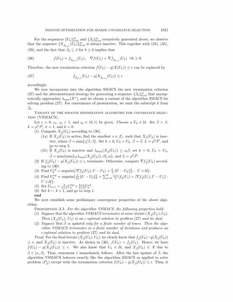
The performance of the methods NSA, SM, and VSM for the randomly generatedinstances are presented in Table 1. The row size n of each sample covariance matrix Σis given in column one. The numbers of iterations of NSA, SM, and VSM are given incolumns two to four, the objective function values are given in columns five to seven,and the CPU times (in seconds) are given in the last three columns, respectively.From Table 1, we conclude that (i) the method SM, namely, the smooth minimizationapproach, outperforms substantially the method NSA, that is, Nesterov’s smooth ap-proximation scheme; and (ii) the method VSM, namely, the variant of the smoothminimization approach, substantially outperforms the other two methods. In addi-tion, we see from this experiment that Nesterov’s smooth minimization approach [19]is generally more appealing than his smooth approximation scheme [21] wheneverthe problem can be solved as an equivalent smooth problem. Nevertheless, we shallmention that the latter approach has a much wider field of application (e.g., see [21]),where the former approach cannot be applied.


Table 1

Comparison of NSA, SM and VSM.

Problem Iter Obj Time

n nsa sm vsm nsa sm vsm nsa sm vsm

50 3657 457 20 −76.399 −76.399 −76.393 49.0 2.7 0.1

100 7629 920 27 −186.717 −186.720 −186.714 900.4 38.4 0.4

150 20358 1455 49 −318.195 −318.194 −318.184 8165.7 188.8 2.0

200 27499 2294 102 −511.246 −511.245 −511.242 26172.5 698.8 9.2

250 45122 3060 128 −3793.255 −3793.256 −3793.257 87298.9 1767.9 19.8

300 54734 3881 161 −3187.163 −3187.171 −3187.172 184798.1 3994.0 45.5

350 64641 4634 182 −2756.717 −2756.734 −2756.734 351460.7 7613.9 83.6

400 74839 5308 176 −3490.640 −3490.667 −3490.667 614237.1 13536.7 116.9

From the above experiment, we have already seen that the method VSM outper-forms substantially two other first-order methods, namely, SM and NSA for solvingproblem (27). In the second experiment, we compare the performance of the methodVSM with the block-coordinate descent methods studied in d’Aspremont et al. [10]and Friedman, Hastie, and Tibshirani [16] on relatively large-scale instances. For con-venience of presentation, we label these two methods BCD1 and BCD2, respectively.The method BCD2 was developed very recently and is a slight variant of the methodBCD1. In particular, each iterate of BCD1 solves a box constrained quadratic pro-gramming by means of interior point methods, but each iterate of BCD2 applies acoordinate descent approach to solving a lasso (l1-regularized) least-squares problem,which is the dual of the box constrained quadratic programming appearing in BCD1.It is worth mentioning that the methods BCD1 and BCD2 are only applicable forsolving problem (16) with α = 0 and β = ∞. Thus, we only compare their per-formance with our method VSM for problem (16) with such α and β. As shown insubsection 3.2, problem (16) with α = 0 and β = ∞ is equivalent to problem (27)with α and β given in (18), and hence it can be solved by applying the method VSMto the latter problem instead.

The code for the method BCD1 was written in MATLAB by d’Aspremont andEl Ghaoui [9], while the code for BCD2 was written in Fortran 90 by Friedman, Hastie,and Tibshirani [15]. The methods BCD1 and VSM terminate once the duality gap isless than ε = 0.1. The original code [15] for BCD2 uses the average absolute changein the approximate solution as the termination criterion. In particular, the averageabsolute change in the approximate solution is evaluated at the end of each cycle con-sisting of n block-coordinate descent iterations, and their code terminates once it isbelow a given accuracy (see [16, p. 6] for details). According to our computational ex-perience, we found that with such a criterion BCD2 is extremely hard to terminate forrelatively large-scale instances (say n = 300) unless a maximum number of iterationsis set. Obviously, it is not easy to choose a suitable maximum number of iterationsfor BCD2. Thus, to be as fair as possible to BCD1 and VSM, we simply replace theirtermination criterion detailed in [15] for BCD2 by the one with the duality gap lessthan ε = 0.1. In other words, the duality gap is computed at the end of each cycleconsisting of n block-coordinate descent iterations, and BCD2 terminates once it isbelow ε = 0.1. It is worth remarking that the cost for computing a duality gap isO(n3) since the inverse of an n×n symmetric matrix is needed. Thus, it is reasonableto compute the duality gap once every n iterations rather than each iteration.

1824 ZHAOSONG LU

Table 2

Comparison of BCD1, BCD2, and VSM.


n bcd1 bcd2 vsm bcd1 bcd2 vsm bcd1 bcd2 vsm

100 124 200 33 −186.522 −186.433 −186.522 22.3 0.1 0.5

200 531 600 109 −449.210 −449.179 −449.209 300.0 1.3 9.5

300 1530 1500 146 −767.615 −767.608 −767.614 2428.2 80.9 48.5

400 2259 2400 154 −1082.679 −1082.651 −1082.677 8402.4 298.7 112.3

500 3050 3500 154 −1402.503 −1402.457 −1402.502 22537.1 640.2 211.5

600 3705 4200 165 −1728.628 −1728.587 −1728.627 48950.4 1215.0 397.6

700 4492 4900 163 −2057.894 −2057.862 −2057.892 92052.7 1972.5 611.1

800 4958 5600 169 −2392.713 −2392.671 −2392.712 147778.9 2872.3 943.2

900 5697 6300 161 −2711.874 −2711.827 −2711.874 219644.3 3593.7 1268.5

1000 6536 7000 161 −3045.808 −3045.768 −3045.808 344687.8 6098.7 1710.0

Table 3

Comparison of BCD2 and VSM.


n bcd2 vsm bcd2 vsm bcd2 vsm

100 200 54 −186.433 −186.435 0.1 0.77

200 1200 239 −449.119 −449.122 2.1 21.6

300 3000 310 −767.525 −767.525 32.1 104.2

400 11778400 321 −1082.592 −1082.589 72000.0 223.3

500 6997000 309 −1402.420 −1402.413 72001.0 395.5

600 4637400 318 −1728.553 −1728.538 72004.0 765.2

700 3215100 310 −2057.823 −2057.804 72005.0 1330.0

800 2307200 309 −2392.644 −2392.623 72003.0 1789.2

900 1846800 289 −2711.806 −2711.784 72024.0 2394.0

1000 1257000 283 −3045.749 −3045.718 72051.0 3115.8

All computations are performed on an Intel Xeon 2.66 GHz machine with RedHat Linux version 8. The performance of the methods BCD1, BCD2, and VSMfor the randomly generated instances are presented in Table 2. The row size n ofeach sample covariance matrix Σ is given in column one. The numbers of iterationsof BCD1, BCD2, and VSM are given in columns two to four, the objective func-tion values are given in columns five to eight, and the CPU times (in seconds) aregiven in the last three columns, respectively. From Table 2, we conclude that bothBCD2 and VSM substantially outperform BCD1. We also observe that our methodVSM outperforms BCD2 for almost all instances except two relatively small-scaleinstances.

In the above experimentation, we compared the performance of BCD2 and VSMfor ε = 0.1. We next compare their performance on the same instances as above andapply the same termination criterion as above except that we set ε = 0.01 and anupper bound of 20 hours computation time (or 72,000 seconds) per instance for bothcodes. The performance of the methods BCD2 and VSM is presented in Table 3. Therow size n of each sample covariance matrix Σ is given in column one. The numbers ofiterations of BCD2 and VSM are given in columns two to three, the objective function


values are given in columns four to five, and the CPU times (in seconds) are givenin the last two columns, respectively. It shall be mentioned that BCD2 and VSMare both feasible methods, and, moreover, (16) and (27) are maximization problems.Therefore for these two methods, the larger the objective function value, the better.From Table 3, we observe that up to accuracy ε = 0.01, the method BCD2 cannotsolve almost all instances within 20 hours except the first three relatively small-scaleones, but our method VSM does solve each of these instances in less than one hourand produces better objective function values for almost all instances except the firstthree relatively small-scale ones. Also, it is interesting to observe that the numberof iterations for VSM nearly doubles as the accuracy parameter ε increases by onedigit, which is even better than the theoretical estimate, which is

√10 according to

Theorem 3.2.

5. Concluding remarks. In this paper, we proposed a smooth optimizationapproach for solving a class of nonsmooth strictly concave maximization problems.We also discussed the application of this approach to sparse covariance selection andproposed a variant of this approach. The computational results showed that thevariant of the smooth optimization approach substantially outperforms the latterone, as well as two other first-order methods studied in d’Aspremont et al. [10] andFriedman et al. [16].

As discussed in subsection 3.3, problem (27) has the same form as (2) and satisfiesall assumptions imposed on problem (2). Moreover, its associated objective functionφ(X,U) = log detX−〈Σ+ρU,X〉 is affine with respect to U for every fixed X ∈ Sn

++.In view of these facts along with the remarks made in section 2, one can observethat problem (27) can be suitably solved by Nesterov’s excessive gap technique [20].Since the iterate complexity and the computational cost per iterate of this techniqueis the same as those of the algorithm SMACS, we expect that the computationalperformance of these two methods for solving (27) is similar. It would be interestingto implement Nesterov’s excessive gap technique [20] and its variant (that is, the onein a similar fashion to the algorithm VSMACS) and compare their computationalperformance with SMACS and VSMACS, respectively.

Though the variant of the smooth optimization approach outperforms substan-tially the smooth optimization approach, we are currently only able to establish somepreliminary convergence properties for it. A possible direction leading to a thoroughproof of its convergence would be to show that the updates on β in the algorithmVSMACS can occur only for a finite number of times. Given that VSMACS isa nonmonotone algorithm, it is, however, highly challenging to analyze the behav-ior of the sequences {Uk} and {Xβ(Uk)} and hence the total number of updates on

β. Interestingly, we observed in our implementation that when β > λmax(X∗), the

sequence {Xβ(Uk)} generated by the algorithm VSMACS satisfies λmax(Xβ(Uk)) ∈[λmax(X

∗), β), where X∗ is the optimal solution of problem (27). Nevertheless, itremains completely open whether or not this holds in general. In addition, the ideasused in the variant of the smooth optimization approach are interesting in their ownright even when viewed as some heuristics. They could also be used to enhancethe practical performance of Nesterov’s first-order methods [19, 21] for solving somegeneral min-max problems.

The codes for the variant of the smooth minimization approach are written inMATLAB and C, which are available online at www.math.sfu.ca/∼zhaosong. TheC code for this method can solve large-scale problems more efficiently, provided theLAPACK package is suitably installed. We will plan to extend these codes for solving

1826 ZHAOSONG LU

more general problems of the form

maxX log detX − 〈Σ, X〉 −∑ij

ωij |Xij |


Xij = 0 ∀(i, j) ∈ Ω

for some set Ω, where ωij = ωji ≥ 0 for all i, j = 1, . . . , n, and 0 ≤ α < β ≤ ∞ aresome fixed bounds on the eigenvalues of the solution.

Acknowledgments. The author would like to thank Prof. Alexandre d’Aspre-mont for a careful discussion on the iteration complexity of Nesterov’s smooth ap-proximation scheme for sparse covariance selection given in [10]. Also, the author isin debt to two anonymous referees for numerous insightful comments and suggestions,which have greatly improved the paper.

REFERENCES

[1] J. Akaike, Information theory and an extension of the maximum likelihood principle, in Pro-ceedings of the Second International Symposium on Information Theory, B. N. Petrov andF. Csaki, eds., Akedemiai Kiado, Budapest, 1973, pp. 267–281.

[2] A. Auslender and M. Teboulle, Interior gradient and proximal methods for convex andconic optimization, SIAM J. Optim., 16 (2006), pp. 697–725.

[3] O. Banerjee, L. El Ghaoui, A. d’Aspremont, and G. Natsoulis, Convex optimizationtechniques for fitting sparse Gaussian graphical models, in ICML ’06: Proceedings of the23rd International Conference on Machine Learning, ACM Press, New York, 2006, pp. 89–96.

[4] J. A. Bilmes, Factored sparse inverse covariance matrices, in Proceedings of IEEE Interna-tional Conference on Acoustics, Speech, and Signal Processing, 2 (2000), pp. 1009–1012.

[5] K. P. Burnham and R. D. Anderson, Multimodel inference. Understanding AIC or BIC inmodel selection, Sociol. Methods Res., 33 (2004), pp. 261–304.

[6] S. S. Chen, D. L. Donoho, and M. A. Saunders, Atomic decomposition by basis pursuit,SIAM J. Sci. Comput., 20 (1998), pp. 33–61.

[7] J. Dahl, V. Roychowdhury, and L. Vandenberghe, Maximum Likelihood Estimation ofGaussian Graphical Models: Numerical Implementation and Topology Selection, manu-script, University of California, Los Angeles, 2004.

[8] J. Dahl, L. Vandenberghe, and V. Roychowdhury, Covariance selection for nonchordalgraphs via chordal embedding, Optim. Methods Softw., 23 (2008), pp. 501–520.

[9] A. d’Aspremont and L. El Ghaoui, Covsel: First order methods for sparse covariance selec-tion, ORFE Department, Princeton University, Princeton, NJ, 2006.

[10] A. d’Aspremont, O. Banerjee, and L. El Ghaoui, First-order methods for sparse covarianceselection, SIAM J. Matrix Anal. Appl., 30 (2008), pp. 56–66.

[11] A. Dempster, Covariance selection, Biometrics, 28 (1972), pp. 157–175.[12] A. Dobra and M. West, Bayesian Covariance Selection, ISDS working paper, Duke Univer-

sity, Durham, NC, 2004.[13] A. Dobra, C. Hans, B. Jones, J. R. Nevins, G. Yao, and M. West, Sparse graphical models

for exploring gene expression data, J. Multivariate Anal., 90 (2004), pp. 196–212.[14] D. L. Donoho and J. Tanner, Sparse nonnegative solutions of underdetermined linear equa-

tions by linear programming, Proc. Natl. Acad. Sci., 102 (2005), pp. 9446–9451.[15] J. Friedman, T. Hastie, and R. Tibshirani, Glasso: Graphical lasso for R, Department of

Statistics, Stanford University, Stanford, CA, 2007.[16] J. Friedman, T. Hastie, and R. Tibshirani, Sparse inverse covariance estimation with the

graphical lasso, Biostatistics, 9 (2008), pp. 432–441.[17] J. Z. Huang, N. Liu, and M. Pourahmadi, Covariance matrix selection and estimation via

penalised normal likelihood, Biometrika, 93 (2006), pp. 85–98.[18] B. Jones, C. Carvalho, C. Dobra, A. Hans, C. Carter, and M. West, Experiments in

stochastic computation for high-dimensional graphical models, Statist. Sci., 20 (2005),pp. 388–400.


[19] Y. E. Nesterov, A method for unconstrained convex minimization problem with the rate ofconvergence O(1/k2), Dokl. Akad. Nauk SSSR, 269 (1983), pp. 543–547 (in Russian).

[20] Y. Nesterov, Excessive gap technique in nonsmooth convex minimization, SIAM J. Optim.,16 (2005), pp. 235–249.

[21] Y. E. Nesterov, Smooth minimization of nonsmooth functions, Math. Programming, 103(2005), pp. 127–152.

[22] Y. Nesterov and A. Nemirovskii, Interior-Point Polynomial Algorithms in Convex Program-ming, SIAM, Philadelphia, 1994.

[23] R. Tibshirani, Regression shrinkage and selection via the lasso, J. Roy. Statist. Soc. Ser. B,58 (1996), pp. 267–288.

[24] L. Vandenberghe, S. Boyd, and S.-P. Wu, Determinant maximization with linear matrixinequality constraints, SIAM J. Matrix Anal. Appl., 19 (1998), pp. 499–533.

[25] M. Yuan and Y. Lin, Model selection and estimation in the Gaussian graphical model,Biometrika, 94 (2007), pp. 19–35.

Documents

SMOOTH OPTIMIZATION APPROACH FOR SPARSE COVARIANCE …people.math.sfu.ca/~zhaosong/ResearchPapers/smoothcovsel.pdf · SMOOTH OPTIMIZATION APPROACH FOR SPARSE COVARIANCE SELECTION