Embed Size (px)
Citation preview

Big & Quic: Sparse Inverse Covariance Estimation for aMillion Variables
Cho-Jui HsiehThe University of Texas at Austin
NIPSLake Tahoe, Nevada
Dec 8, 2013
Joint work with M. Sustik, I. Dhillon, P. Ravikumar and R. Poldrack
Cho-Jui Hsieh The University of Texas at Austin Big & Quic: Sparse Inverse Covariance Estimation

FMRI Brain Analysis
Goal: Reveal functional connections between regions of the brain.(Sun et al, 2009; Smith et al, 2011; Varoquaux et al, 2010; Ng et al, 2011)
p = 228, 483 voxels.
Figure from (Varoquaux et al, 2010)Cho-Jui Hsieh The University of Texas at Austin Big & Quic: Sparse Inverse Covariance Estimation

Other Applications
Gene regulatory network discovery:
(Schafer & Strimmer 2005; Andrei & Kendziorski 2009; Menendez etal, 2010; Yin and Li, 2011)
Financial Data Analysis:
Model dependencies in multivariate time series (Xuan & Murphy, 2007).Sparse high dimensional models in economics (Fan et al, 2011).
Social Network Analysis / Web data:
Model co-authorship networks (Goldenberg & Moore, 2005).Model item-item similarity for recommender system(Agarwal et al, 2011).
Climate Data Analysis (Chen et al., 2010).
Signal Processing (Zhang & Fung, 2013).
Anomaly Detection (Ide et al, 2009).
Cho-Jui Hsieh The University of Texas at Austin Big & Quic: Sparse Inverse Covariance Estimation

Inverse Covariance Estimation
Given: n i.i.d. samples {y1, . . . , yn}, yi ∈ Rp, yi ∼ N (µ,Σ),
An example – Chain graph: yj = 0.5yj−1 +N (0, 1)
Σ =
1.33 0.67 0.33 0.170.67 1.33 0.67 0.330.33 0.67 1.33 0.670.17 0.33 0.67 1.33
, Σ−1 =
1 −0.5 0 0−0.5 1.25 −0.5 0
0 −0.5 1.25 −0.50 0 −0.5 1
Conditional independence is reflected as zeros in Σ−1:
Σ−1ij = 0⇔ yi and yj are conditionally independent given other variables.
Cho-Jui Hsieh The University of Texas at Austin Big & Quic: Sparse Inverse Covariance Estimation

L1-regularized inverse covariance selection
Goal: Estimate the inverse covariance matrix in the high dimensionalsetting: p(# variables)� n(# samples)
Add `1 regularization – a sparse inverse covriance matrix is preferred.
The `1-regularized Maximum Likelihood Estimator:
Σ−1 = arg minX�0
{− log det X + tr(SX )︸ ︷︷ ︸
negative log likelihood
+λ‖X‖1
}= arg min
X�0f (X ),
where ‖X‖1 =∑n
i ,j=1 |Xij |.
The problem appears hard to solve:
Non-smooth log-determinant program.Number of parameters scale quadratically with number of variables.
Cho-Jui Hsieh The University of Texas at Austin Big & Quic: Sparse Inverse Covariance Estimation

L1-regularized inverse covariance selection
Goal: Estimate the inverse covariance matrix in the high dimensionalsetting: p(# variables)� n(# samples)
Add `1 regularization – a sparse inverse covriance matrix is preferred.
The `1-regularized Maximum Likelihood Estimator:
Σ−1 = arg minX�0
{− log det X + tr(SX )︸ ︷︷ ︸
negative log likelihood
+λ‖X‖1
}= arg min
X�0f (X ),
where ‖X‖1 =∑n
i ,j=1 |Xij |.The problem appears hard to solve:
Non-smooth log-determinant program.Number of parameters scale quadratically with number of variables.
Cho-Jui Hsieh The University of Texas at Austin Big & Quic: Sparse Inverse Covariance Estimation

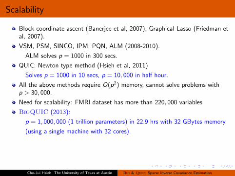
Scalability
Block coordinate ascent (Banerjee et al, 2007), Graphical Lasso (Friedman etal, 2007).
VSM, PSM, SINCO, IPM, PQN, ALM (2008-2010).
ALM solves p = 1000 in 300 secs.
QUIC: Newton type method (Hsieh et al, 2011)
Solves p = 1000 in 10 secs, p = 10, 000 in half hour.
All the above methods require O(p2) memory, cannot solve problems withp > 30, 000.
Need for scalability: FMRI dataset has more than 220, 000 variables
BigQUIC (2013):
p = 1, 000, 000 (1 trillion parameters) in 22.9 hrs with 32 GBytes memory
(using a single machine with 32 cores).
Cho-Jui Hsieh The University of Texas at Austin Big & Quic: Sparse Inverse Covariance Estimation
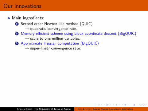
Our innovations
Main Ingredients:1 Second-order Newton-like method (QUIC)
→ quadratic convergence rate.2 Memory-efficient scheme using block coordinate descent (BigQUIC)
→ scale to one million variables.3 Approximate Hessian computation (BigQUIC)
→ super-linear convergence rate.
Cho-Jui Hsieh The University of Texas at Austin Big & Quic: Sparse Inverse Covariance Estimation

QUIC – proximal Newton method
Split smooth and non-smooth terms: f (X ) = g(X ) + h(X ), where
g(X ) = − log det X + tr(SX ) and h(X ) = λ‖X‖1.
Form quadratic approximation for g(Xt + ∆):
gXt (∆) = tr((S −Wt)∆) + (1/2) vec(∆)T (Wt ⊗Wt) vec(∆)
− log det Xt + tr(SXt),
where Wt = (Xt)−1 = ∂∂X log det(X ) |X=Xt .
Define the generalized Newton direction:
Dt = arg min∆
gXt (∆) + λ‖Xt + ∆‖1.
Solve by coordinate descent (Hsieh et al, 2011) or other methods (Olsen et al, 2012).
Cho-Jui Hsieh The University of Texas at Austin Big & Quic: Sparse Inverse Covariance Estimation

Coordinate Descent Updates
Use coordinate descent to solve:
arg minD{gX (D) + λ‖X + D‖1}.
Closed form solution for each coordinate descent update:
Dij ← −c + S(c − b/a, λ/a),
where S(z , r) = sign(z) max{|z | − r , 0} is the soft-thresholdingfunction, a = W 2
ij + WiiWjj , b = Sij −Wij + wTi Dwj , and c = Xij + Dij .
The main cost is in computing wTi Dwj ,
where wi ,wj are i-th and j-th columns of W = X−1.
Cho-Jui Hsieh The University of Texas at Austin Big & Quic: Sparse Inverse Covariance Estimation

Algorithm
QUIC: QUadratic approximation for sparse Inverse Covariance estimation
Input: Empirical covariance matrix S , scalar λ, initial X0.
For t = 0, 1, . . .1 Variable selection: select a free set of m� p2 variables.2 Use coordinate descent to find descent direction:
Dt = arg min∆ fXt (Xt + ∆) over set of free variables, (A Lasso problem.)3 Line Search: use an Armijo-rule based step-size selection to get α s.t.
Xt+1 = Xt + αDt is
positive definite,satisfies a sufficient decrease condition f (Xt + αDt) ≤ f (Xt) + ασ∆t .
(Cholesky factorization of Xt + αDt)
Cho-Jui Hsieh The University of Texas at Austin Big & Quic: Sparse Inverse Covariance Estimation

Difficulties in Scaling QUIC
Consider the case that p ≈ 1million, m = ‖Xt‖0 ≈ 50million.
Coordinate descent requires Xt and W = X−1t ,
needs O(p2) storageneeds O(mp) computation per sweep, where m = ‖Xt‖0
Line search (compute determinant using Cholesky factorization).
needs O(p2) storageneeds O(p3) computation
Cho-Jui Hsieh The University of Texas at Austin Big & Quic: Sparse Inverse Covariance Estimation
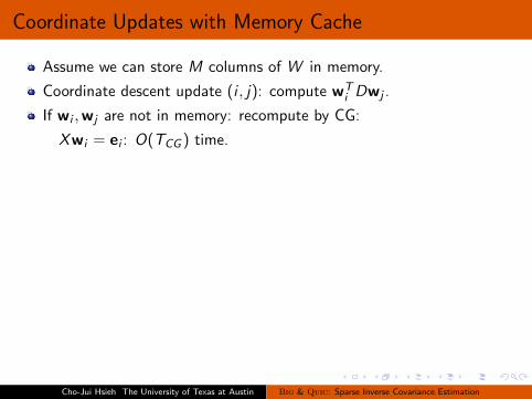
Coordinate Updates with Memory Cache
Assume we can store M columns of W in memory.
Coordinate descent update (i , j): compute wTi Dwj .
If wi ,wj are not in memory: recompute by CG:
Xwi = ei : O(TCG ) time.
Cho-Jui Hsieh The University of Texas at Austin Big & Quic: Sparse Inverse Covariance Estimation

Coordinate Updates with Memory Cache
w1,w2,w3,w4 stored in memory.
Cho-Jui Hsieh The University of Texas at Austin Big & Quic: Sparse Inverse Covariance Estimation

Coordinate Updates with Memory Cache
Cache hit, do not need to recompute wi ,wj .
Cho-Jui Hsieh The University of Texas at Austin Big & Quic: Sparse Inverse Covariance Estimation

Coordinate Updates with Memory Cache
Cache miss, recompute wi ,wj .
Cho-Jui Hsieh The University of Texas at Austin Big & Quic: Sparse Inverse Covariance Estimation

Coordinate Updates – ideal case
Want to find update sequence that minimizes number of cache misses:
probably NP Hard.
Our strategy: update variables block by block.
The ideal case: there exists a partition {S1, . . . ,Sk} such that all freesets are in diagonal blocks:
Only requires p column evaluations.
Cho-Jui Hsieh The University of Texas at Austin Big & Quic: Sparse Inverse Covariance Estimation
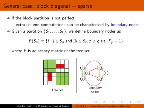
General case: block diagonal + sparse
If the block partition is not perfect:
extra column computations can be characterized by boundary nodes.
Given a partition {S1, . . . ,Sk}, we define boundary nodes as
B(Sq) ≡ {j | j ∈ Sq and ∃i ∈ Sz , z 6= q s.t. Fij = 1},
where F is adjacency matrix of the free set.
Cho-Jui Hsieh The University of Texas at Austin Big & Quic: Sparse Inverse Covariance Estimation

Graph Clustering Algorithm
The number of columns to be computed in one sweep is
p +∑q
|B(Sq)|.
Can be upper bounded by
p +∑q
|B(Sq)| ≤ p +∑z 6=q
∑i∈Sz ,j∈Sq
Fij .
Use Graph Clustering (METIS or Graclus) to find the partition.
Example: on fMRI dataset (p = 0.228 million) with 20 blocks,
random partition: need 1.6 million column computations.
graph clustering: need 0.237 million column computations.
Cho-Jui Hsieh The University of Texas at Austin Big & Quic: Sparse Inverse Covariance Estimation
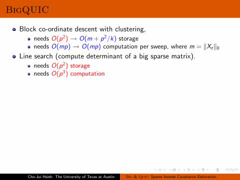
BigQUIC
Block co-ordinate descent with clustering,
needs O(p2) → O(m + p2/k) storageneeds O(mp) → O(mp) computation per sweep, where m = ‖Xt‖0
Line search (compute determinant of a big sparse matrix).
needs O(p2) storageneeds O(p3) computation
Cho-Jui Hsieh The University of Texas at Austin Big & Quic: Sparse Inverse Covariance Estimation
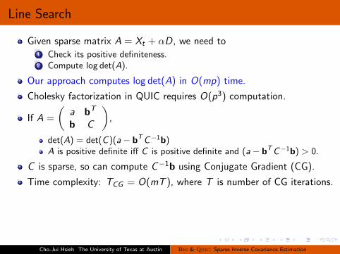
Line Search
Given sparse matrix A = Xt + αD, we need to1 Check its positive definiteness.2 Compute log det(A).
Our approach computes log det(A) in O(mp) time.
Cholesky factorization in QUIC requires O(p3) computation.
If A =
(a bT
b C
),
det(A) = det(C )(a− bTC−1b)A is positive definite iff C is positive definite and (a− bTC−1b) > 0.
C is sparse, so can compute C−1b using Conjugate Gradient (CG).
Time complexity: TCG = O(mT ), where T is number of CG iterations.
Cho-Jui Hsieh The University of Texas at Austin Big & Quic: Sparse Inverse Covariance Estimation

BigQUIC
Block co-ordinate descent with clustering,
needs O(p2) → O(m + p2/k) storageneeds O(mp) → O(mp) computation per sweep, where m = ‖Xt‖0
Line search (compute determinant of a big sparse matrix).
needs O(p2)→ O(p) storageneeds O(p3) → O(mp) computation
Cho-Jui Hsieh The University of Texas at Austin Big & Quic: Sparse Inverse Covariance Estimation

Algorithm
BigQUIC
Input: Samples Y , scalar λ, initial X0.
For t = 0, 1, . . .1 Variable selection: select a free set of m� p2 variables.2 Construct a partition by clustering.3 Run block coordinate descent to find descent direction:
Dt = arg min∆ fXt (Xt + ∆) over set of free variables.4 Line Search: use an Armijo-rule based step-size selection to get α s.t.
Xt+1 = Xt + αDt is
positive definite,satisfies a sufficient decrease condition f (Xt + αDt) ≤ f (Xt) + ασ∆t .
(Schur complement with conjugate gradient method. )
Cho-Jui Hsieh The University of Texas at Austin Big & Quic: Sparse Inverse Covariance Estimation

BigQUIC Convergence Analysis
Recall W = X−1.
When each wi is computed by CG (Xwi = ei ):
The gradient ∇ijg(X ) = Sij −Wij on free set can be computed once andstored in memory.Hessian (wT
i Dwj in coordinate updates) needs to be repeatedlycomputed.
To reduce the time overhead, Hessian should be computedapproximately.
Theorem: the convergence rate is quadratic if‖X wi − ei‖ = O(‖∇S f (Xt)‖) , where
∇Sij f (X ) =
{∇ijg(X ) + sign(Xij)λ if Xij 6= 0,
sign(∇ijg(X )) max(|∇ijg(X )| − λ, 0) if Xij = 0.
Cho-Jui Hsieh The University of Texas at Austin Big & Quic: Sparse Inverse Covariance Estimation
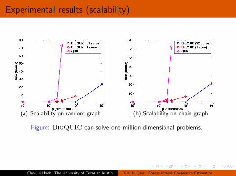
Experimental results (scalability)
(a) Scalability on random graph (b) Scalability on chain graph
Figure: BigQUIC can solve one million dimensional problems.
Cho-Jui Hsieh The University of Texas at Austin Big & Quic: Sparse Inverse Covariance Estimation

Experimental results
BigQUIC is faster even for medium size problems.
Figure: Comparison on FMRI data with a p = 20000 subset (maximum dimensionthat previous methods can handle).
Cho-Jui Hsieh The University of Texas at Austin Big & Quic: Sparse Inverse Covariance Estimation

Results on FMRI dataset
228,483 voxels, 518 time points.
λ = 0.6 =⇒ average degree 8, BigQUIC took 5 hours.
λ = 0.5 =⇒ average degree 38, BigQUIC took 21 hours.
Findings:
Voxels with large degree were generally found in the gray matter.Can detect meaningful brain modules by modularity clustering.
Cho-Jui Hsieh The University of Texas at Austin Big & Quic: Sparse Inverse Covariance Estimation

Conclusions
BigQUIC: Memory efficient quadratic approximation method forsparse inverse covariance estimation.
Our contributions:Computing Newton direction:
Coordinate descent → block coordinate descent with clustering.Memory complexity: O(p2) → O(m + p2/k).Time complexity: O(mp) → O(mp).
Line search (computing determinant of a big sparse matrix)
Cholesky factorization → Schur complement with conjugate gradientmethod.Memory complexity: O(p2) → O(p).Time complexity: O(p3) → O(mp).
Inexact Hessian computation with super-linear convergence.
Cho-Jui Hsieh The University of Texas at Austin Big & Quic: Sparse Inverse Covariance Estimation

References
[1] C. J. Hsieh, M. Sustik, I. S. Dhillon, P. Ravikumar, and R. Poldrack. BIG & QUIC: Sparseinverse covariance estimation for a million variables . NIPS (oral presentation), 2013.[2] C. J. Hsieh, M. Sustik, I. S. Dhillon, and P. Ravikumar. Sparse Inverse Covariance MatrixEstimation using Quadratic Approximation. NIPS, 2011.[3] C. J. Hsieh, I. S. Dhillon, P. Ravikumar, A. Banerjee. A Divide-and-Conquer Procedure forSparse Inverse Covariance Estimation. NIPS, 2012.[4] P. A. Olsen, F. Oztoprak, J. Nocedal, and S. J. Rennie. Newton-Like Methods for SparseInverse Covariance Estimation. Optimization Online, 2012.[5] O. Banerjee, L. El Ghaoui, and A. d’Aspremont Model Selection Through Sparse MaximumLikelihood Estimation for Multivariate Gaussian or Binary Data. JMLR, 2008.[6] J. Friedman, T. Hastie, and R. Tibshirani. Sparse inverse covariance estimation with thegraphical lasso. Biostatistics, 2008.[7] L. Li and K.-C. Toh. An inexact interior point method for l1-reguarlized sparse covarianceselection. Mathematical Programming Computation, 2010.[8] K. Scheinberg, S. Ma, and D. Glodfarb. Sparse inverse covariance selection via alternatinglinearization methods. NIPS, 2010.[9] K. Scheinberg and I. Rish. Learning sparse Gaussian Markov networks using a greedycoordinate ascent approach. Machine Learning and Knowledge Discovery in Databases, 2010.
Cho-Jui Hsieh The University of Texas at Austin Big & Quic: Sparse Inverse Covariance Estimation


![0.15in ECE 18-898G: Special Topics in Signal Processing ...users.ece.cmu.edu/.../ece18898g_graphical_model.pdf · [1]”Sparse inverse covariance estimation with the graphical lasso,”](https://img.dokumen.tips/doc/110x75/5f640d1e6d738d660c0fccfe/015in-ece-18-898g-special-topics-in-signal-processing-usersececmueduece18898ggraphicalmodelpdf.jpg)