SMIP15 Seminar Proceedings GROUND-MOTION … the recordings were ... (only the profiles for KiK-net stations had profiles to the three greatest values of z). (Modified from Figure

SMIP15 Seminar Proceedings

1

GROUND-MOTION PREDICTION EQUATIONS: PAST, PRESENT, AND FUTURE (The 2014 William Joyner Lecture)

David M. Boore

U.S. Geological Survey, Menlo Park, CA, United States ([email protected])

Abstract

Ground-motion prediction equations (GMPEs) typically give amplitudes of ground motion as a function of distance from earthquakes of a particular magnitude. They are the foundations on which the seismic hazard maps used in building codes are built, they provide motions for the design of critical structures, and they and the databases used in their derivation conveniently summarize a large amount of information about the seismic waves radiated from earthquakes. The development of GMPEs requires knowledge of many aspects of seismology, including data acquisition, data processing, source physics, the determination of crustal structure, the effects of that structure on the propagation of seismic waves, the measurement and characterization of the geotechnical properties near the Earth’s surface, and the nonlinear response of soils to strong shaking. Generally, GMPEs are developed for three regions: active crustal regions (ACR), stable continental regions (SCR), and subduction zones (SZ). Most GMPEs in ACRs and SZs are based on empirical analysis of observed ground motion, while those in data-poor areas such as SCRs rely primarily on simulations of ground shaking. As data sets increase and theoretical simulations improve, previous GMPEs are revised and new ones are proposed. As a result, many hundreds of GMPEs have been published, and more are on their way. As an example of the current state-of-practice for GMPEs in ACRs, I will discuss a recent multi-year project undertaken by the Pacific Earthquake Engineering Research Center (PEER). The future is bound to bring more data, but most of these data will be for magnitudes and distances where present GMPEs are well constrained by existing data, at least in ACRs. Significant gaps will continue to exist in our knowledge of ground shaking in certain distance and magnitude ranges for ACRs and for SCRs in general. For this reason, combinations of simulated and observed motions will be used to create future GMPEs.

Introduction

Ground-motion prediction equations (GMPEs) provide ground motions for various ground-motion intensity measures (GMIMs) as a function of various predictor variables, such as a measure of earthquake magnitude, distance from the earthquake to the site, and a characterization of the geology near the site. The predicted motions include a complete statistical distribution, not just a mean value. GMPEs are widely used in earthquake engineering to provide design motions for critical structures as well as being the foundation on which the design maps in modern building codes are built. This talk concentrates in GMPEs developed as part of the Pacific Earthquake Engineering Research Center’s NGA-West2 project (Bozorgnia et al., 2014). GMPEs were developed both for horizontal component and for vertical component


2

ground motions. A critical part of that project was the construction of a well-vetted global database of GMIMs and associated metadata (Ancheta et al., 2014). In addition to their engineering uses, the GMPEs developed from the database are a convenient summary of the overall magnitude and distance behavior of a very large number of ground-motion recordings, and as such, they are useful in assessing the magnitude scaling of ground motion, which is intimately related to the source processes of earthquakes.

These notes accompany the Joyner Lecture presented at the SMIP15 meeting in Davis, California, on 22 October 2015.

The PEER NGA-West2 Database

The Pacific Earthquake Engineering Center (PEER) NGA-West2 database, developed by Ancheta et al. (2014), contains 21,336 three-component recordings from 599 shallow crustal earthquakes in active tectonic regions around the world. Great care was taken in developing the database: the recordings were processed in a uniform and consistent manner to provide high-quality seismic intensity measures and metadata, such as source and site properties. The metadata were evaluated by several teams of researchers to ensure consistency in view of the different regions and methods used to obtain the metadata by various researchers.

The ground-motion intensity measures used for the NGA-West2 database are 5%-damped pseudo-absolute response spectral acceleration (PSA), peak ground acceleration (PGA), and peak ground velocity (PGV). The horizontal components were combined to produce a measure that is independent of the orientation of the instruments as installed at a site. The GMPEs for the NGA-West2 project use the measure rotd50 (Boore, 2010), which represents the median value of PSA over all possible instrument orientations (rotd100 represents the maximum PSA for a pair of records overall all possible orientations; there is a relatively robust, period-dependent relation between rotd50 and rotd100).

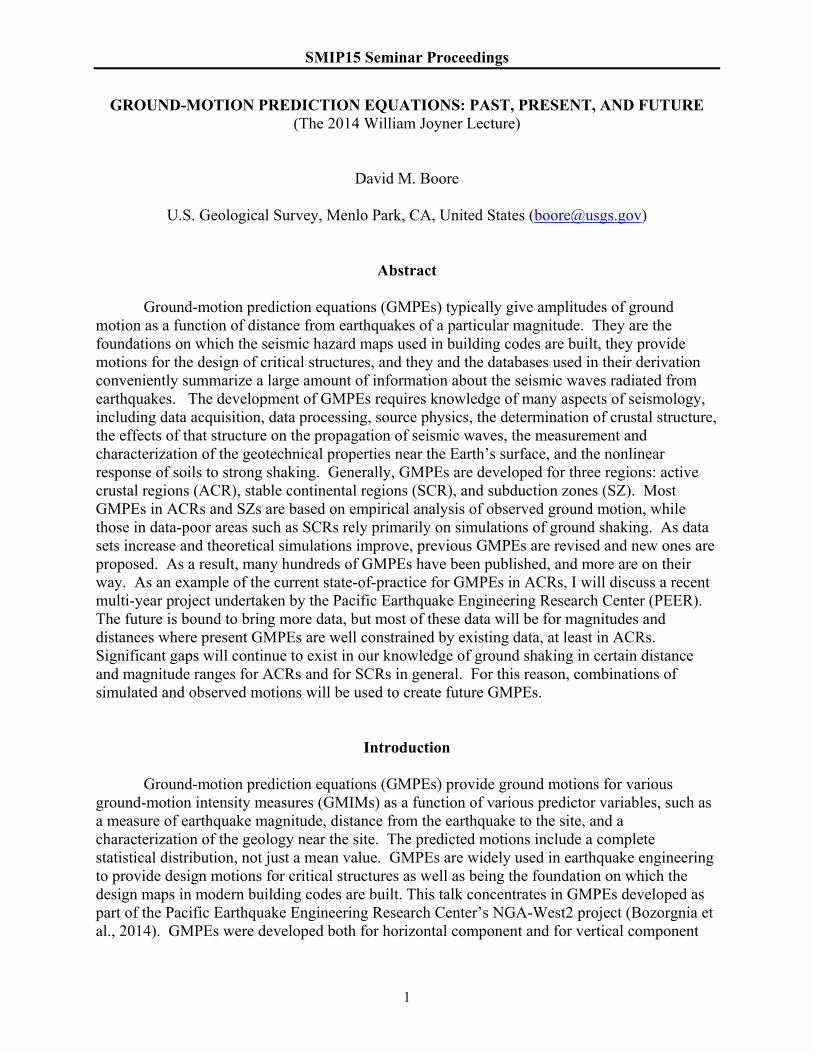
The most common metadata used in developing GMPEs are measures of distance, magnitude, and site geology. In the NGA-West2 database, the magnitude measure is moment magnitude M (Hanks and Kanamori, 1979). The two main distance measures used in the NGA-West2 project are RUPR and JBR , defined in Figure 1 (along with a number of other possible

measures of distance from a site to a fault rupture surface).


3

Figure 1. Some distance measures. The most commonly used measures in modern GMPEs are

RUPR , the closest distance to the rupture surface, and JBR , the closest horizontal

distance to the surface projection of the rupture surface (“JB” for Joyner and Boore, who introduced this measure in Joyner and Boore, 1981). 0.0JBR for sites over the

fault.

The site geology is characterized in the NGA-West2 project by the time-weighted average of the shear-wave velocity from the surface to 30 m ( 30SV ). While it has been argued that

such a velocity may not be representative of the shear-wave velocities at deeper depths, which can affect longer period motions, Boore et al. (2011) show that there is a good correlation of 30SV

and the shear-wave velocity averaged to depths significantly greater than 30 m (Figure 2).


4

Figure 2. Scatterplot of 30SV and SZV from shear-wave velocity profiles for six averaging depths z

(only the profiles for KiK-net stations had profiles to the three greatest values of z). (Modified from Figure 10 in Boore et al., 2011, which contains formal correlation coefficients for each graph; these range from 0.98 for 50 mz to 0.79 for 600 mz .)

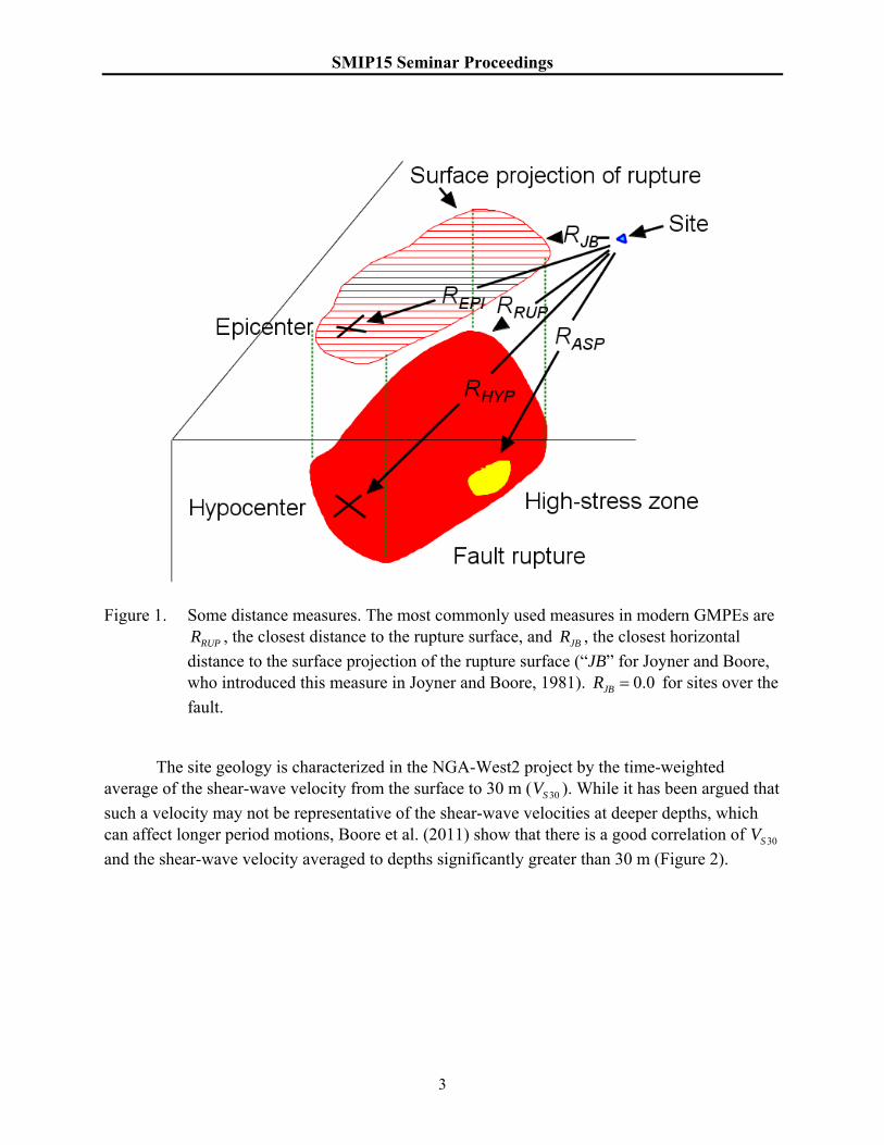
The NGA-West2 database contains PSA for periods from 0.01 s to 20 s. The magnitude-

distance distribution of the PSA are shown in Figure 3 for OSCT of 1.0 s and 10.0 s, with the data

differentiated by earthquake source mechanism. It is clear from Figure 3 that there are many fewer data for the long-period oscillator (and in fact, the fall-off in available data begins at a period of about 1.0 s, as shown in Boore et al., 2014); this is an inevitable consequence of the signal-to-noise characteristics of ground motions recorded on accelerographs (which provide the bulk of the data for the larger earthquakes).


5

Figure 3. Magnitude-distance distribution of data from the PEER NGA-West2 database,

differentiated by fault type (SS=StrikeSlip; NS=NormalSlip; RS=ReverseSlip). The distributions are shown for two oscillator periods, 1.0 s and 10.0 s.

What the Data Tell Us about Choosing the Functions for Ground-Motion Prediction Equations

The functions used in GMPEs are guided by what is expected from physical grounds and

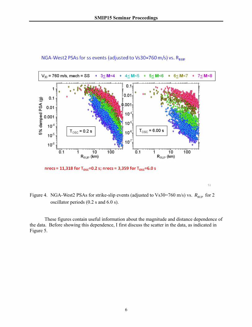
also by what the data show. In this section I show various aspects of the NGA-W2 data used by BSSA14 that must be captured by the functions. To provide an overview of the magnitude and distance dependence of the global data, Figure 4 shows PSA values for four periods plotted against distance, with magnitude bins indicated by symbols of different color. The data are from strikeslip earthquakes, adjusted to a common 30SV value of 760 m/s using the site response

equations of Seyhan and Stewart (2014). This figure shows a number of robust features related to magnitude and distance scaling of ground motions for a wide range of magnitudes and distances, without assuming any functional forms for this dependence (aside from the 30SV adjustment).

The motions are shown for two oscillator periods: 0.2 s and 6.0 s.


6

Figure 4. NGA-West2 PSAs for strike-slip events (adjusted to Vs30=760 m/s) vs. RUPR for 2

oscillator periods (0.2 s and 6.0 s).

These figures contain useful information about the magnitude and distance dependence of the data. Before showing this dependence, I first discuss the scatter in the data, as indicated in Figure 5.


7

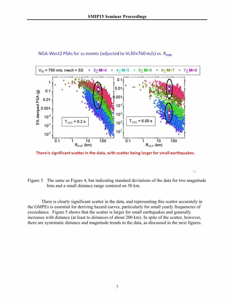
Figure 5. The same as Figure 4, but indicating standard deviations of the data for two magnitude

bins and a small distance range centered on 50 km.

There is clearly significant scatter in the data, and representing this scatter accurately in the GMPEs is essential for deriving hazard curves, particularly for small yearly frequencies of exceedance. Figure 5 shows that the scatter is larger for small earthquakes and generally increases with distance (at least to distances of about 200 km). In spite of the scatter, however, there are systematic distance and magnitude trends in the data, as discussed in the next figures.


8

Figure 6. The same as Figure 4, but highlighting the saturation at close distances for a single

magnitude and all periods.

For a single magnitude and for all periods the motions tend to saturate for large earthquakes, that is, they approach a constant value, as the distance from the fault rupture to the observation point decreases. This can only be concluded definitively for large magnitudes, for which the rupture approaches the ground surface and therefore the distance measure used in Figure 6 can approach 0.0. Smaller earthquakes do not reach the surface, and therefore surface observations cannot be used to infer whether or not the motions near the rupture surfaces of small earthquakes saturate.


9

Figure 7. The same as Figure 4, but showing the distance bands to be used to illustrate the

scaling of motions at a fixed distance (next figure).

At any fixed distance the ground motion increases with magnitude in a nonlinear fashion, with a tendency to saturate for large magnitudes, particularly for shorter period motions. The overall magnitude scaling increases with increasing period, but it is smaller at short distances than at longer distances. For short periods and close distances there appears to be almost complete saturation for the motions from large earthquakes.


10

To emphasize the magnitude scaling for a fixed distance, Figure 8 shows that scaling for

data in a small distance range centered on 50 km.

Figure 8. The scaling of motions at two periods as a function of magnitude. Note that the

shorter period motions exhibit more saturation of the scaling at large magnitudes than do the longer period motions.

Note shown here is that theoretical predictions for a standard seismological model of the ground motion are in good agreement with this magnitude scaling (Figures 17, 18, and 18 in Boore, 2013).


11

For a given period and magnitude the median ground motions decay with distance; this

decay shows curvature at greater distances on the log-log plot used in Figure 9. This decay can be parameterized as exp( )RUP RUPR R , where the terms in the numerator and denominator are

similar to the decay from a point source due to anelastic attenuation and geometrical spreading, respectively. In log-log plots the anelastic attenuation produces the curvature at greater distances, and the geometrical spreading produces the linear decay at closer distances. Careful inspection of Figure 9 shows that the apparent geometrical spreading decreases as magnitude increases. In addition to the dependencies shown in the preceding figures, the equations need to capture site dependence of the motion (including basin depth dependence and nonlinear response), earthquake type, hanging wall, depth to top of rupture, etc. This results in what seems to be complicated equations.

Figure 9. This shows both the steepening of attenuation as distance increases and the magnitude

dependence of the attenuation with distances.


12

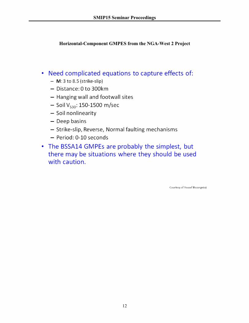
Horizontal-Component GMPES from the NGA-West 2 Project


13

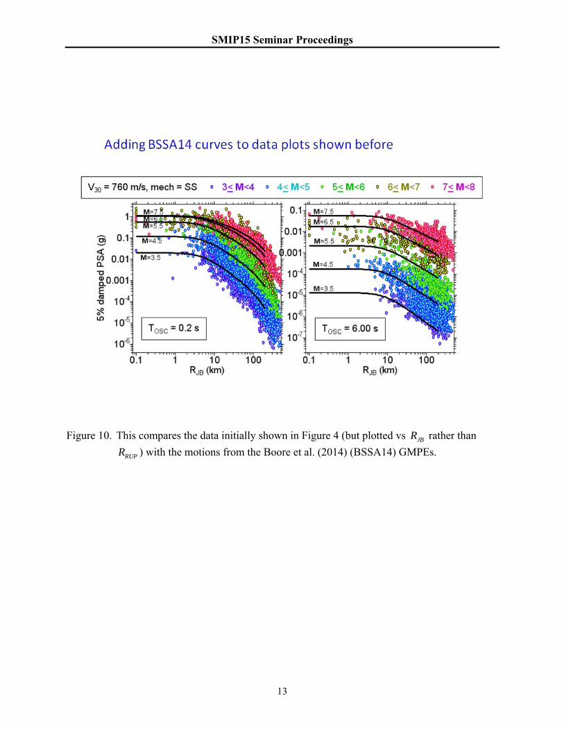
Figure 10. This compares the data initially shown in Figure 4 (but plotted vs JBR rather than

RUPR ) with the motions from the Boore et al. (2014) (BSSA14) GMPEs.


14

A few comparisons of the GMPEs resulting from the NGA-West2 project are given in Figures 11 and 12.

Figure 11. Comparing predictions from the five NGA-West2 GMPEs.


15

Figure 12. Comparing magnitude scaling from the five NGA-West2 GMPEs for a fixed distance

(30 km).


16

Use of GMPEs in Building Codes

The following figures illustrate the probabilistic seismic hazard results from the U.S.G.S. National Seismic Hazard Mapping (NSHM) program. Underlying the results are the GMPEs from the previous NGA-West project, published in 2008 (the latest NSHM results are for 2014 and use the NGA-West2 GMPEs; the NSHM web site, however, does not allow for generation of the deaggregation figures, so I used the 2008 NSHM results; the essential points to be made would not change if the more recent results were used.

Figure 13. A hazard map for the US, from the National Seismic Hazard Mapping program of the

USGS.


17

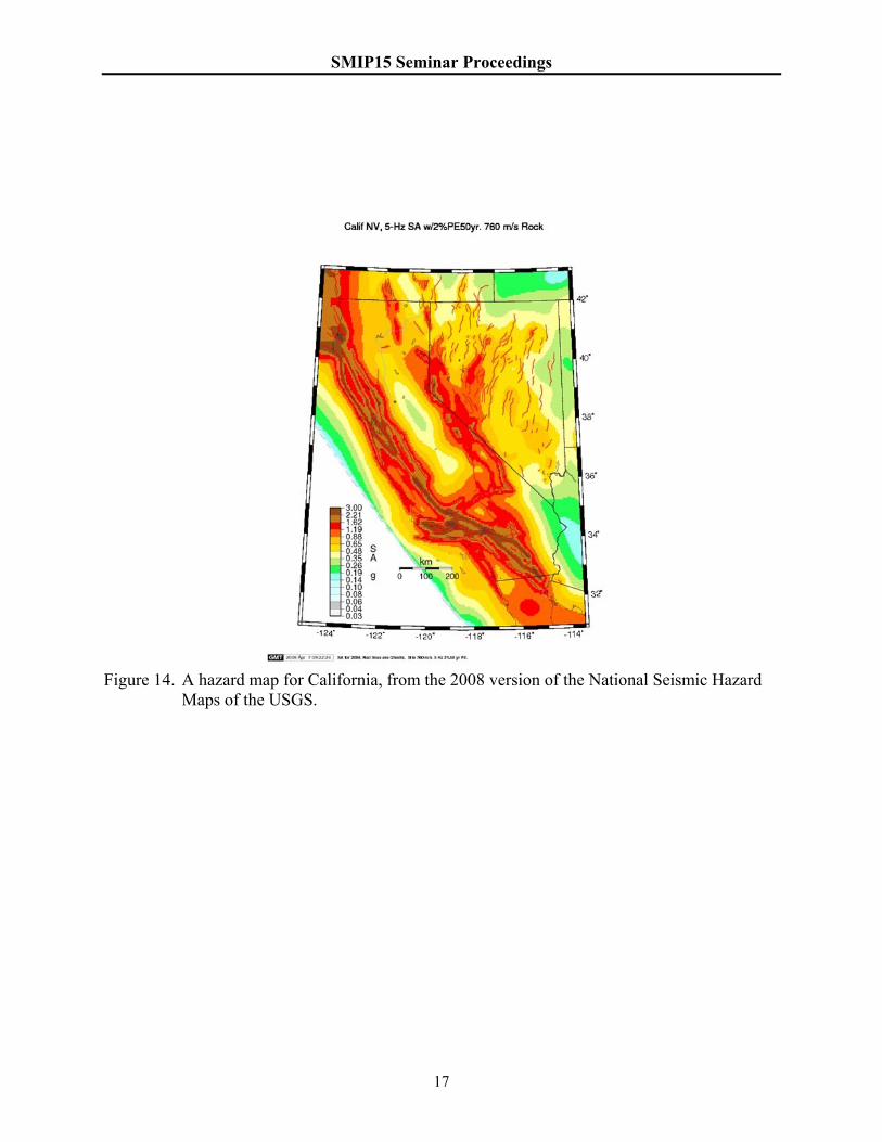
Figure 14. A hazard map for California, from the 2008 version of the National Seismic Hazard

Maps of the USGS.


18

Figure 15. The deaggregation for Davis, California, from the 2008 USGS National Seismic

Hazard Mapping web site. The period is 0.2 s. with a frequency of exceedance of 2% in 50 years. The colors refer to the number of standard deviation about the median ground motion that contribute to the hazard at the chosen frequency of exceedance.


19

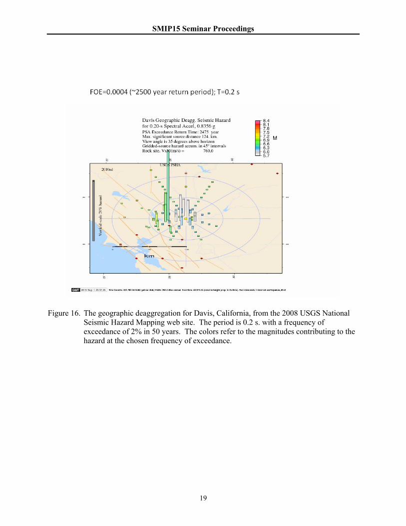
Figure 16. The geographic deaggregation for Davis, California, from the 2008 USGS National

Seismic Hazard Mapping web site. The period is 0.2 s. with a frequency of exceedance of 2% in 50 years. The colors refer to the magnitudes contributing to the hazard at the chosen frequency of exceedance.


20

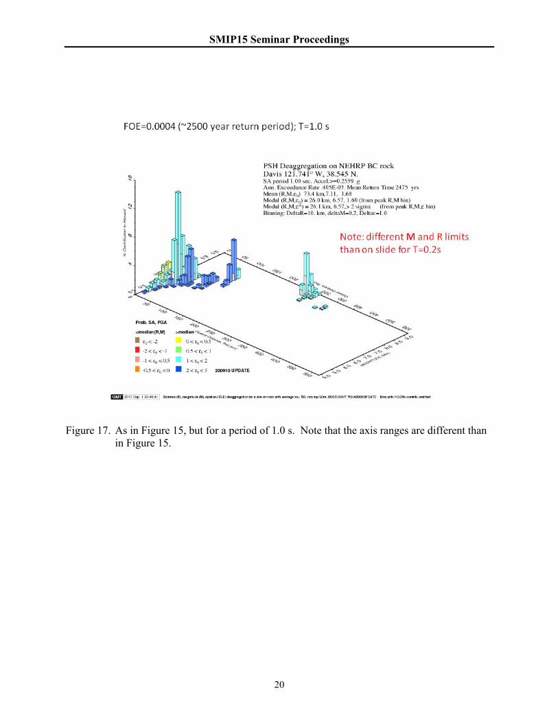
Figure 17. As in Figure 15, but for a period of 1.0 s. Note that the axis ranges are different than

in Figure 15.


21

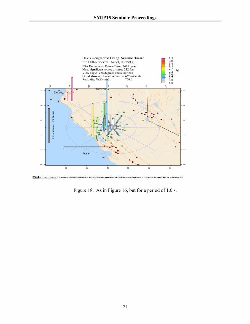
Figure 18. As in Figure 16, but for a period of 1.0 s.


22

References

Ancheta, T.D., R.B. Darragh, J.P. Stewart, E. Seyhan, W.J. Silva, B.S.J. Chiou, K.E. Wooddell,

R.W. Graves, A.R. Kottke, D.M. Boore, T. Kishida, and J.L. Donahue (2014). NGA-West2 database, Earthquake Spectra 30, 989–1005.

Baltay, A. S. and T. C. Hanks (2014). Understanding the magnitude dependence of PGA and PGV in NGA-West2 data, Bull. Seismol. Soc. Am. 104, 2851–2865.

Boore, D.M. (2010). Orientation-independent, non geometric-mean measures of seismic intensity from two horizontal components of motion, Bull. Seismol. Soc. Am. 100, 1830–1835.

Boore, D.M. (2014). What do data used to develop ground-motion prediction equations tell us about motions near faults?, Pure and Applied Geophysics 171, 3023–3043.

Boore, D.M., E.M. Thompson, and H. Cadet (2011). Regional correlations of 30SV and velocities

averaged over depths less than and greater than 30 m, Bull. Seismol. Soc. Am. 101, 3046–3059.

Boore, D.M., J.P. Stewart, E. Seyhan, and G.M. Atkinson (2014). NGA-West 2 equations for predicting PGA, PGV, and 5%-Damped PSA for shallow crustal earthquakes, Earthquake Spectra 30, 1057–1085.

Bozorgnia, Y., N.A. Abrahamson, L. Al Atik, T.D. Ancheta, G.M. Atkinson, J.W. Baker, A. Baltay, D.M. Boore, K.W. Campbell, B.S.-J. Chiou, R. Darragh, S. Day, J. Donahue, R. W. Graves, N. Gregor, T. Hanks, I.M. Idriss, R. Kamai, T. Kishida, A. Kottke, S.A. Mahin, S. Rezaeian, B. Rowshandel, E. Seyhan, S. Shahi, T. Shantz, W. Silva, P. Spudich, J.P. Stewart, J. Watson-Lamprey, K. Wooddell, and R. Youngs (2014). NGA-West2 Research Project, Earthquake Spectra 30, 973–987.

Hanks, T.C. and H. Kanamori (1979). A moment magnitude scale, J. Geophys. Res. 84, 2348–2350.

Joyner, W.B. and D.M. Boore (1981). Peak horizontal acceleration and velocity from strong-motion records including records from the 1979 Imperial Valley, California, earthquake, Bull. Seismol. Soc. Am. 71, 2011—2038.

Seyhan, E. and J.P. Stewart (2014). Semi-empirical nonlinear site amplification from NGA-West 2 data and simulations, Earthquake Spectra 30, 1241–1256.

Documents

SMIP15 Seminar Proceedings GROUND-MOTION … the recordings were ... (only the profiles for KiK-net stations had profiles to the three greatest values of z). (Modified from Figure